1

Separation Science - Chromatography Unit

Thomas Wenzel

Department of Chemistry

Bates College, Lewiston ME 04240

twenzel@bates.edu

The following textual material is designed to accompany a series of in-class problem sets that

develop many of the fundamental aspects of chromatography.

TABLE OF CONTENTS

Liquid-Liquid Extraction 2

Chromatography – Background 6

Introduction 6

Distribution Isotherms 14

Adsorption Compared to Partition as a Separation Mechanism 16

Broadening of Chromatographic Peaks 21

Longitudinal Diffusion Broadening 23

Eddy Diffusion (Multipath) Broadening in Chromatography 25

Stationary Phase Mass Transport Broadening 30

Mobile Phase Mass Transport Broadening 39

Concluding Comments 43

Fundamental Resolution Equation 46

N- Number of Theoretical Plates 46

– Selectivity Factor 47

k – Retention or Capacity Factor 48

Liquid Chromatographic Separation Methods 51

Steric Exclusion Chromatography 53

Ion-Exchange Chromatography 58

Bonded-Phase Liquid Chromatography 66

Gas Chromatographic Separation Methods 70

Detection Methods 74

Capillary Electrophoresis 78

Appendix 1. Derivation of the Fundamental Resolution Equation 87

2

LIQUID-LIQUID EXTRACTION

Before examining chromatographic separations, it is useful to consider the separation process in

a liquid-liquid extraction. Certain features of this process closely parallel aspects of

chromatographic separations. The basic procedure for performing a liquid-liquid extraction is to

take two immiscible phases, one of which is usually water and the other of which is usually an

organic solvent. The two phases are put into a device called a separatory funnel, and compounds

in the system will distribute between the two phases. There are two terms used for describing

this distribution, one of which is called the distribution coefficient (DC), the other of which is

called the partition coefficient (DM).

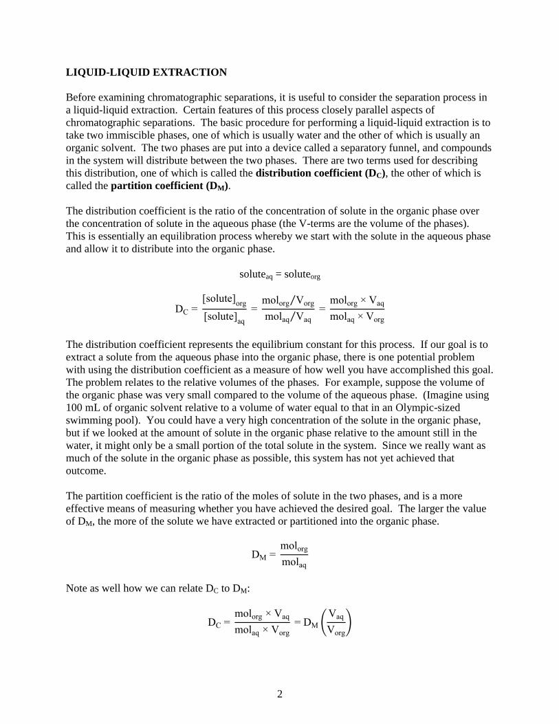
The distribution coefficient is the ratio of the concentration of solute in the organic phase over

the concentration of solute in the aqueous phase (the V-terms are the volume of the phases).

This is essentially an equilibration process whereby we start with the solute in the aqueous phase

and allow it to distribute into the organic phase.

soluteaq = soluteorg

DC = [solute]

org

[solute]aq

= molorg Vorg⁄

molaq Vaq⁄ =

molorg × Vaq

molaq × Vorg

The distribution coefficient represents the equilibrium constant for this process. If our goal is to

extract a solute from the aqueous phase into the organic phase, there is one potential problem

with using the distribution coefficient as a measure of how well you have accomplished this goal.

The problem relates to the relative volumes of the phases. For example, suppose the volume of

the organic phase was very small compared to the volume of the aqueous phase. (Imagine using

100 mL of organic solvent relative to a volume of water equal to that in an Olympic-sized

swimming pool). You could have a very high concentration of the solute in the organic phase,

but if we looked at the amount of solute in the organic phase relative to the amount still in the

water, it might only be a small portion of the total solute in the system. Since we really want as

much of the solute in the organic phase as possible, this system has not yet achieved that

outcome.

The partition coefficient is the ratio of the moles of solute in the two phases, and is a more

effective means of measuring whether you have achieved the desired goal. The larger the value

of DM, the more of the solute we have extracted or partitioned into the organic phase.

DM = molorg

molaq

Note as well how we can relate DC to DM:

DC = molorg × Vaq

molaq × Vorg

= DM (Vaq

Vorg

)

3

From experience you have probably had in your organic chemistry lab, you know that the

approach that is often used in liquid-liquid extraction is to add some organic phase, shake the

mixture, and remove the organic phase. A fresh portion of the organic phase is then added to

remove more of the solute in a second extraction. As we will see shortly, this distribution of a

solute between two immiscible phases forms the basis of chromatographic separations as well.

Next we want to examine some general types of extraction procedures that are commonly used.

The first is a classic example of an extraction procedure that can be used to separate acids, bases,

and neutrals.

An aqueous sample contains a complex mixture of organic compounds, all of which are at

trace concentrations. The compounds can be grouped into broad categories of organic

acids, organic bases and neutral organics. The desire is to have three solutions at the end,

each in methylene chloride, one of which contains only the organic acids, the second

contains only the organic bases, and the third contains only the neutrals. Devise an

extraction procedure that would allow you to perform this bulk separation of the three

categories of organic compounds.

Two things to remember:

Ionic substances are more soluble in water than in organic solvents.

Neutral substances are more soluble in organic solvents than in water.

The key to understanding how to do this separation relates to the effect that pH will have on the

different categories of compounds.

Neutrals – Whether the pH is acidic or basic, these will remain neutral under all circumstances.

Organic acids – RCOOH

At very acidic pH values (say a pH of around 1) – these are fully protonated and neutral

At basic pH values (say a pH of around 13) – these are fully deprotonated and anionic

Organic bases – R3N

At very acidic pH values (say a pH of around 1) – these are protonated and cationic

At very basic pH values (say a pH of around 13) – these are not protonated and neutral

Step 1: Lower the pH of the water using concentrated hydrochloric acid.

Neutrals – neutral

Acids – neutral

Bases – cationic

Extract with methylene chloride – the neutrals and acids go into the methylene chloride, the

bases stay in the water.

4

Step 2: Remove the water layer from step (1), adjust the pH back to a value of 13 using a

concentrated solution of sodium hydroxide, shake against methylene chloride, and we now have

a solution of the organic bases in methylene chloride. (SOLUTION 1 – ORGANIC BASES IN

METHYLENE CHLORIDE)

Step 3: Take the methylene chloride layer from step (1) and shake this against an aqueous layer

with a pH value of 13 (adjusted to that level using a concentrated solution of sodium hydroxide).

Neutrals – neutral

Organic acids – anionic

The neutrals stay in the methylene chloride layer. (SOLUTION 2: NEUTRALS IN

METHYLENE CHLORIDE) The acids go into the water layer.

Step 4. Take the water layer from Step (3), lower the pH to a value of 1 using concentrated

hydrochloric acid, shake against methylene chloride, and the neutral organic acids are now

soluble in the methylene chloride (SOLUTION 3: ORGANIC ACIDS IN METHYLENE

CHLORIDE).

Devise a way to solubilize the organic anion shown below in the organic solvent of a two-

phase system in which the second phase is water. As a first step to this problem, show what

might happen to this compound when added to such a two-phase system.

This compound will align itself right along the interface of the two layers. The non-polar C18

group is hydrophobic and will be oriented into the organic phase. The polar carboxylate group is

hydrophilic and will be right at the interface with the aqueous phase.

One way to solubilize this anion in the organic phase is to add a cation with similar properties.

In other words, if we added an organic cation that has a non-polar R group, this would form an

ion pair with the organic anion. The ion pair between the two effectively shields the two charged

groups and allows the pair to dissolve in an organic solvent. Two possible organic cations that

could be used in this system are cetylpyridinium chloride or tetra-n-butylammonium chloride.

5

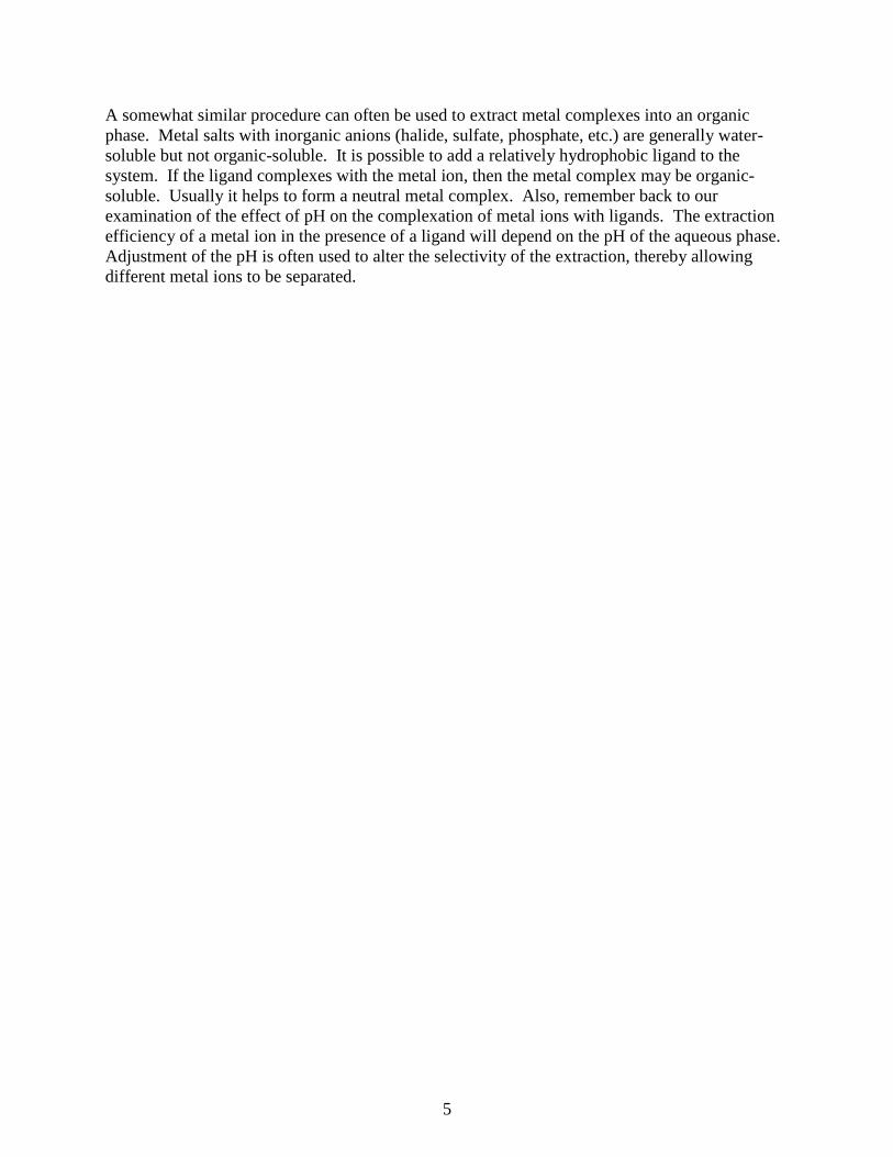
A somewhat similar procedure can often be used to extract metal complexes into an organic

phase. Metal salts with inorganic anions (halide, sulfate, phosphate, etc.) are generally water-

soluble but not organic-soluble. It is possible to add a relatively hydrophobic ligand to the

system. If the ligand complexes with the metal ion, then the metal complex may be organic-

soluble. Usually it helps to form a neutral metal complex. Also, remember back to our

examination of the effect of pH on the complexation of metal ions with ligands. The extraction

efficiency of a metal ion in the presence of a ligand will depend on the pH of the aqueous phase.

Adjustment of the pH is often used to alter the selectivity of the extraction, thereby allowing

different metal ions to be separated.

6

CHROMATOGRAPHY – BACKGROUND

Chromatography refers to a group of methods that are used as a way of separating mixtures of

compounds into their individual components. The basic set up of a chromatographic system is to

have two phases, one stationary and one mobile. A compound, which we will usually call the

solute, is introduced into the system, and essentially has a choice. If it is attracted to the mobile

phase (has van der Waal attractions to the mobile phase), it will move through the system with

the mobile phase. If it is attracted to the stationary phase, it will lag behind. It’s easy to imagine

some solute compounds with some degree of attraction for both phases, such that these move

through the system with some intermediate rate of travel.

The first report of a chromatographic application was by Mikhail Tswett, a chemist from Estonia,

in 1903. (A list of important literature articles is provided at the end). Undoubtedly other people

had observed chromatography taking place, but no one until Tswett recognized its applicability

for the separation of mixtures in chemistry. Tswett was interested in separating the pigments in

plants. He packed a glass column that might have been comparable to a buret with starch,

mashed up the plant and extracted the pigments into a solvent, loaded the solution onto the top of

the starch column, and ran a mobile phase through the starch. Eventually he saw different color

bands separate on the column, hence the term chromatography. Rather than eluting the colored

bands off of the column, he stopped it, used a rod to push out the starch filling, divided up the

bands of color, and extracted the individual pigments off the starch using an appropriate solvent.

Twsett used a solid stationary phase (starch) and a liquid mobile phase.

Chromatographic systems can use either a gas or liquid as the mobile phase. Chromatographic

systems can use either a solid or liquid as the stationary phase. A solid stationary phase is easy

to imagine, as we have already seen for Tswett’s work. Another common example is to use

paper as the solid (actually, paper is made from a compound called cellulose). The sample is

spotted onto the paper as shown in Figure 1a, and the bottom of the piece of paper is dipped into

an appropriate liquid (note that the spot is above the liquid – Figure 1b). The liquid mobile

phase moves up the paper by capillary action, and components of the mixture can separate into

different spots depending on their relative attraction to the cellulose or chemicals that make up

the liquid (Figure 1c).

Figure 1. Paper chromatography

Sample Spot

Solvent Front

(a) (b) (c)

7

Another type of chromatography that you may be familiar with is thin layer chromatography

(TLC). This is very similar to paper chromatography, although the stationary phase is usually a

coating of small particles of a material known as silica gel (silica gel is a polymer with the

formula SiO2, although a bit later we will talk in more detail about the exact chemical nature of

this material) on a glass or plastic plate. Similarly, we could take these silica gel particles and

pack them into a glass column, and then flow a liquid through the column. If we used some gas

pressure to force the liquid through the silica gel column more quickly, we would have a

common technique known as flash chromatography that synthetic chemists use to separate

relatively large amounts of materials they have prepared. Another common solid to use in

column chromatography is alumina (Al2O3 is the general formula, although we will say more

later about its exact chemical nature).

These methods we have just been talking about are examples of liquid-solid chromatography. If

we used gas as the mobile phase, injected either a gaseous sample or liquid sample into a high

temperature zone that flash volatilized it, with some solid as the stationary phase (there are a

range of possible materials we could use here), we could perform gas-solid chromatography. If

we thought about how a solute compound would interact with such a solid stationary phase, we

would realize that it must essentially “stick” to the surface by some intermolecular (van der

Waal) forces. This sticking process in chromatography is known as adsorption.

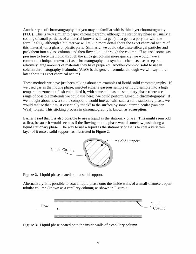
Earlier I said that it is also possible to use a liquid as the stationary phase. This might seem odd

at first, because it would seem as if the flowing mobile phase would somehow push along a

liquid stationary phase. The way to use a liquid as the stationary phase is to coat a very thin

layer of it onto a solid support, as illustrated in Figure 2.

Figure 2. Liquid phase coated onto a solid support.

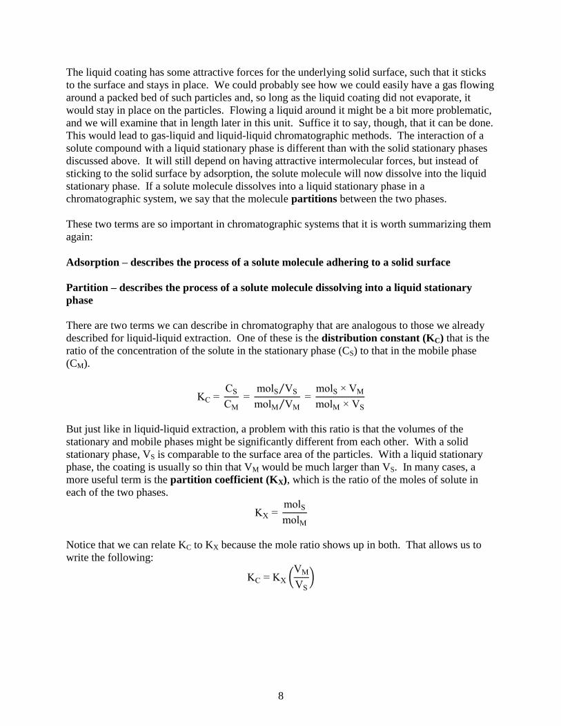
Alternatively, it is possible to coat a liquid phase onto the inside walls of a small-diameter, open-

tubular column (known as a capillary column) as shown in Figure 3.

Figure 3. Liquid phase coated onto the inside walls of a capillary column.

Solid Support

Liquid Coating

Flow Liquid

Coating

8

The liquid coating has some attractive forces for the underlying solid surface, such that it sticks

to the surface and stays in place. We could probably see how we could easily have a gas flowing

around a packed bed of such particles and, so long as the liquid coating did not evaporate, it

would stay in place on the particles. Flowing a liquid around it might be a bit more problematic,

and we will examine that in length later in this unit. Suffice it to say, though, that it can be done.

This would lead to gas-liquid and liquid-liquid chromatographic methods. The interaction of a

solute compound with a liquid stationary phase is different than with the solid stationary phases

discussed above. It will still depend on having attractive intermolecular forces, but instead of

sticking to the solid surface by adsorption, the solute molecule will now dissolve into the liquid

stationary phase. If a solute molecule dissolves into a liquid stationary phase in a

chromatographic system, we say that the molecule partitions between the two phases.

These two terms are so important in chromatographic systems that it is worth summarizing them

again:

Adsorption – describes the process of a solute molecule adhering to a solid surface

Partition – describes the process of a solute molecule dissolving into a liquid stationary

phase

There are two terms we can describe in chromatography that are analogous to those we already

described for liquid-liquid extraction. One of these is the distribution constant (KC) that is the

ratio of the concentration of the solute in the stationary phase (CS) to that in the mobile phase

(CM).

KC = CS

CM

= molS VS⁄

molM VM⁄ =

molS × VM

molM × VS

But just like in liquid-liquid extraction, a problem with this ratio is that the volumes of the

stationary and mobile phases might be significantly different from each other. With a solid

stationary phase, VS is comparable to the surface area of the particles. With a liquid stationary

phase, the coating is usually so thin that VM would be much larger than VS. In many cases, a

more useful term is the partition coefficient (KX), which is the ratio of the moles of solute in

each of the two phases.

KX = molS

molM

Notice that we can relate KC to KX because the mole ratio shows up in both. That allows us to

write the following:

KC = KX (VM

VS

)

9

There are also some other fundamental figures of merit that we often use when discussing

chromatographic separations. The first is known as the selectivity factor (). In order to

separate two components of a mixture, it is essential that the two have different distribution or

partition coefficients (note, it does not matter which one you use since the volume terms will

cancel if KC is used). The separation factor is the ratio of these two coefficients, and is always

written so that it is greater than or equal to one. K2 represents the distribution coefficient for the

later eluting of the two components.

α = K2

K1

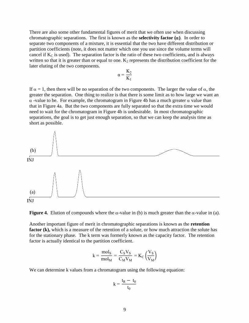
If = 1, then there will be no separation of the two components. The larger the value of , the

greater the separation. One thing to realize is that there is some limit as to how large we want an

-value to be. For example, the chromatogram in Figure 4b has a much greater value than

that in Figure 4a. But the two components are fully separated so that the extra time we would

need to wait for the chromatogram in Figure 4b is undesirable. In most chromatographic

separations, the goal is to get just enough separation, so that we can keep the analysis time as

short as possible.

Figure 4. Elution of compounds where the -value in (b) is much greater than the -value in (a).

Another important figure of merit in chromatographic separations is known as the retention

factor (k), which is a measure of the retention of a solute, or how much attraction the solute has

for the stationary phase. The k term was formerly known as the capacity factor. The retention

factor is actually identical to the partition coefficient.

k = molS

molM =

CSVS

CMVM

= KC (VS

VM

)

We can determine k values from a chromatogram using the following equation:

k = tR − t0

t0

INJ

INJ

(a)

(b)

10

Figure 5. Chromatographic information used to calculate the k value for a peak.

As seen in Figure 5, the term tR is the retention time of the compound of interest, whereas t0

refers to the retention time of an unretained compound (the time it takes a compound with no

ability to partition into or adsorb onto the stationary phase to move through the column). Since t0

will vary from column to column, the form of this equation represents a normalization of the

retention times to t0.

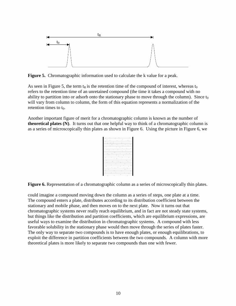
Another important figure of merit for a chromatographic column is known as the number of

theoretical plates (N). It turns out that one helpful way to think of a chromatographic column is

as a series of microscopically thin plates as shown in Figure 6. Using the picture in Figure 6, we

Figure 6. Representation of a chromatographic column as a series of microscopically thin plates.

could imagine a compound moving down the column as a series of steps, one plate at a time.

The compound enters a plate, distributes according to its distribution coefficient between the

stationary and mobile phase, and then moves on to the next plate. Now it turns out that

chromatographic systems never really reach equilibrium, and in fact are not steady state systems,

but things like the distribution and partition coefficients, which are equilibrium expressions, are

useful ways to examine the distribution in chromatographic systems. A compound with less

favorable solubility in the stationary phase would then move through the series of plates faster.

The only way to separate two compounds is to have enough plates, or enough equilibrations, to

exploit the difference in partition coefficients between the two compounds. A column with more

theoretical plates is more likely to separate two compounds than one with fewer.

tR

t0

11

We can determine the number of plates for a compound as shown in Figure 7.

N = 16 (tR

W)

2

Figure 7. Chromatographic information used to determine N for a column.

W is the width of the peak where it intersects with the baseline. The important thing to

remember is to use the same units when measuring W and tR (e.g., distance in cm on a plot, time

in seconds, elution volume in mL – which is common in liquid chromatography). It should be

pointed out that a column will have a set number of plates that will not vary much from

compound to compound. The reason for this is that a compound with a longer retention time will

exhibit a larger peak width, such that the ratio term is correcting for these two effects.

If we determine the number of plates for a column, dividing the column length (L) by the number

of plates leads to the height equivalent to a theoretical plate (H). Note that the smaller the

value of H the better. It actually turns out the H is the important figure of merit for a column.

H = L

N

The chromatograms in Figure 8 show the distinction between a column with a smaller value of H

(Figure 8a) and one with a much larger value of H (Figure 8b).

Figure 8. Chromatograms for a column with (a) a smaller value of H and (b) a larger value of H.

INJ

INJ

(b)

(a)

INJ

tR

W

12

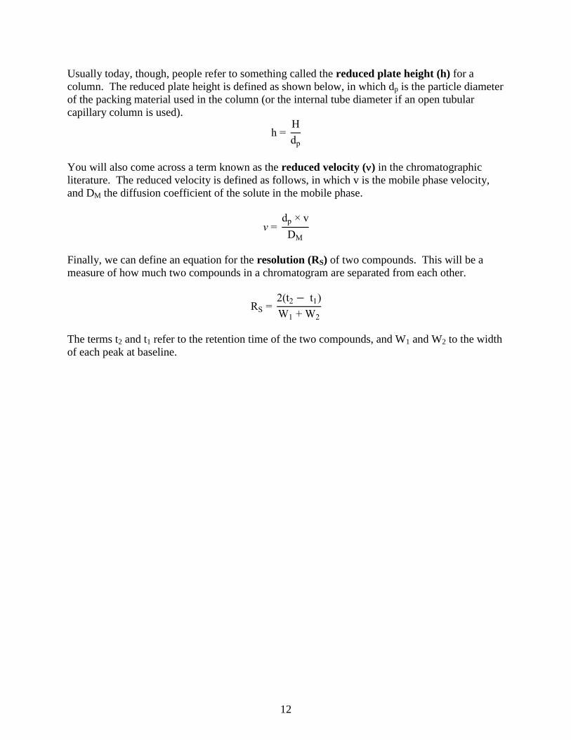
Usually today, though, people refer to something called the reduced plate height (h) for a

column. The reduced plate height is defined as shown below, in which dp is the particle diameter

of the packing material used in the column (or the internal tube diameter if an open tubular

capillary column is used).

h = H

dp

You will also come across a term known as the reduced velocity () in the chromatographic

literature. The reduced velocity is defined as follows, in which v is the mobile phase velocity,

and DM the diffusion coefficient of the solute in the mobile phase.

v = dp × v

DM

Finally, we can define an equation for the resolution (RS) of two compounds. This will be a

measure of how much two compounds in a chromatogram are separated from each other.

RS = 2(t2 − t1)

W1 + W2

The terms t2 and t1 refer to the retention time of the two compounds, and W1 and W2 to the width

of each peak at baseline.

13

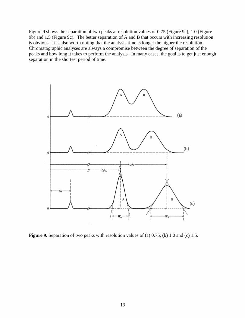
Figure 9 shows the separation of two peaks at resolution values of 0.75 (Figure 9a), 1.0 (Figure

9b) and 1.5 (Figure 9c). The better separation of A and B that occurs with increasing resolution

is obvious. It is also worth noting that the analysis time is longer the higher the resolution.

Chromatographic analyses are always a compromise between the degree of separation of the

peaks and how long it takes to perform the analysis. In many cases, the goal is to get just enough

separation in the shortest period of time.

Figure 9. Separation of two peaks with resolution values of (a) 0.75, (b) 1.0 and (c) 1.5.

14

Distribution Isotherms (Isotherm means constant temperature):

We have used the distribution and partition coefficients as ways to express the distribution of a

molecule between the mobile and stationary phase. Note that these equations take the form of

equilibrium expressions, and that KC is a constant for the distribution of a solute compound

between two particular phases. (KX depends on the relative volumes of the two phases.)

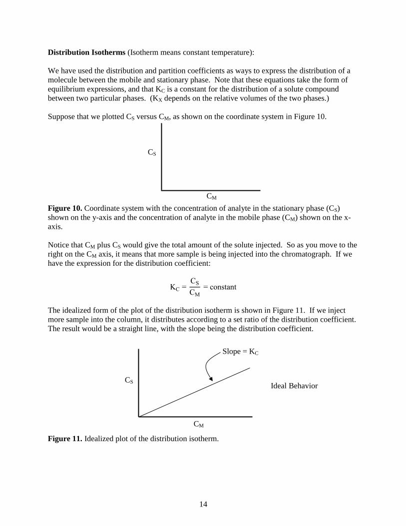
Suppose that we plotted CS versus CM, as shown on the coordinate system in Figure 10.

Figure 10. Coordinate system with the concentration of analyte in the stationary phase (CS)

shown on the y-axis and the concentration of analyte in the mobile phase (CM) shown on the x-

axis.

Notice that CM plus CS would give the total amount of the solute injected. So as you move to the

right on the CM axis, it means that more sample is being injected into the chromatograph. If we

have the expression for the distribution coefficient:

KC = CS

CM

= constant

The idealized form of the plot of the distribution isotherm is shown in Figure 11. If we inject

more sample into the column, it distributes according to a set ratio of the distribution coefficient.

The result would be a straight line, with the slope being the distribution coefficient.

Figure 11. Idealized plot of the distribution isotherm.

CS

CM

CS

CM

Slope = KC

Ideal Behavior

15

If we examine this in more detail, though, we will realize that the volume of stationary phase is

some fixed quantity, and is usually substantially less than the volume of the mobile phase. It is

possible to saturate the stationary phase with solute, such that no more can dissolve. In that case,

the curve would show the behavior shown in Figure 12, a result known as the Langmuir

isotherm (Langmuir was a renowned surface scientist and a journal of the American Chemical

Society on surface science is named in his honor). If we get a region of Langmuir behavior, we

have saturated the stationary phase or overloaded the capacity of the column.

Figure 12. Plot of the Langmuir isotherm.

We might also ask whether you could ever get the following plot, which is called anti-Langmuir

behavior.

Figure 13. Plot of the anti-Langmuir isotherm.

There are actually two ways this could happen. One is if the solute dissolves in the stationary

phase, creating a mixed phase that then allows a higher solubility of the solute. This behavior is

not commonly observed. Another way that this can occur is in gas chromatography if too large

or concentrated a sample of solute is injected. At a fixed temperature, a volatile compound has a

specific vapor pressure. This vapor pressure can never be exceeded. If the vapor pressure is not

exceeded, all of the compound can evaporate. If too high a concentration of compound is

injected such that it would exceed the vapor pressure if all evaporates, some evaporates into the

gas phase but the rest remains condensed as a liquid. If this happens, it is an example of anti-

Langmuir behavior because it appears as if more is in the stationary phase (the condensed

droplets of sample would seem to be in the stationary phase because they are not moving).

Langmuir Isotherm

CS

CM

CS

CM

Anti-Langmuir Isotherm

16

The last question we need to consider is what these forms of non-ideal behavior would do to the

shape of a chromatographic peak. From laws of diffusion, it is possible to derive that an “ideal”

chromatographic peak will have a symmetrical (Gaussian) shape. Either form of overloading

will lead to asymmetry in the peaks. This can cause either fronting or tailing as shown in

Figure 14. The Langmuir isotherm, which results from overloading of the stationary phase, leads

to peak tailing. Anti-Laugmuir behavior leads to fronting.

Figure 14. Representation of a chromatographic peak exhibiting ideal peak shape, fronting, and

tailing.

Adsorption Compared to Partition as a Separation Mechanism

If we go back now and consider Tswett’s first separation, we see that he used solid starch as the

stationary phase, and so solutes exhibited an adsorption to the surface of the starch. A useful

thing to consider is the nature of the chemical groups on the surface of starch. Starch is a

carbohydrate comprised of glucose units. The glucose functionality of starch is shown below,

and we see that the surface is comprised of highly polar hydroxyl groups.

Glucose

Silica gel (SiO2) and alumina (Al2O3) were mentioned previously as two other common solid

phases. If we examine the structure of silica gel, in which each silicon atom is attached to four

oxygen atoms in a tetrahedral arrangement (this corresponds to two silicon atoms sharing each of

the oxygen atoms), we run into a problem when you try to create a surface for this material. If

we have an oxygen atom out on the edge, we would then need to attach a silicon atom, which

necessitates more oxygen atoms. We end up with a dilemma in which we can never wrap all of

these around on each other and only make something with the formula SiO2. Some of these

groups are able to do this and some of the surface of silica gel consists of what are known as

siloxane (Si–O–Si) groups. But many of the outer oxygen atoms cannot attach to another silicon

atom and are actually hydroxyl or silanol (Si–OH) groups.

–Si–O–Si– –Si–OH

Siloxane units Silanol units

INJ INJ INJ Ideal Fronting Tailing

17

What we notice is that the surface of silica gel consists of very polar hydroxyl groups. It turns

out that the same thing will occur for the surface of alumina.

If we consider a solute molecule (S), and have it adsorb to the surface of silica gel, we could

write the following equation to represent the process of adsorption.

Si–OH + S Si–OH - - - S

With any reaction we can talk about its enthalpy and entropy. So in this case, we could talk

about the enthalpy of adsorption (HADS). Suppose now we took one solute molecule and

millions of surface silanols, and went through one by one and measured HADS for this one

solute molecule with each of these millions of surface silanols. The question is whether we

would get one single HADS value for each of the measurements. Hopefully it might seem

intuitive to you that we would not get an identical value for each of these individual processes.

Instead, it seems like what we would really get is a distribution of values. There would be one

value that is most common with other less frequent values clustered around it. For some reason,

some silanol sites might be a bit more active because of differences in their surrounding

microenvironment, whereas others might be a bit less active. Suppose we entered all these

measurements in a spreadsheet and then plotted them as a histogram with number of

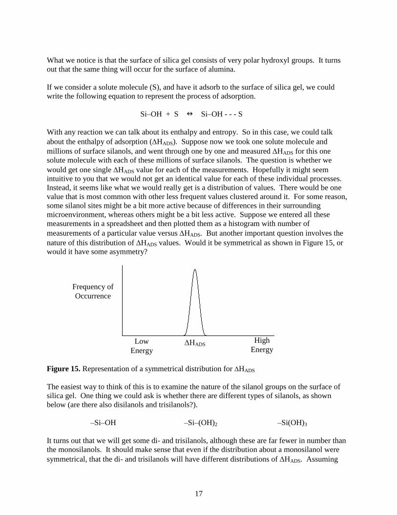
measurements of a particular value versus HADS. But another important question involves the

nature of this distribution of HADS values. Would it be symmetrical as shown in Figure 15, or

would it have some asymmetry?

Figure 15. Representation of a symmetrical distribution for HADS

The easiest way to think of this is to examine the nature of the silanol groups on the surface of

silica gel. One thing we could ask is whether there are different types of silanols, as shown

below (are there also disilanols and trisilanols?).

–Si–OH –Si–(OH)2 –Si(OH)3

It turns out that we will get some di- and trisilanols, although these are far fewer in number than

the monosilanols. It should make sense that even if the distribution about a monosilanol were

symmetrical, that the di- and trisilanols will have different distributions of HADS. Assuming

Frequency of

Occurrence

Low

Energy

High

Energy ΔHADS

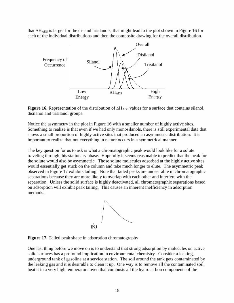
18

that HADS is larger for the di- and trisilanols, that might lead to the plot shown in Figure 16 for

each of the individual distributions and then the composite drawing for the overall distribution.

Figure 16. Representation of the distribution of HADS values for a surface that contains silanol,

disilanol and trisilanol groups.

Notice the asymmetry in the plot in Figure 16 with a smaller number of highly active sites.

Something to realize is that even if we had only monosilanols, there is still experimental data that

shows a small proportion of highly active sites that produced an asymmetric distribution. It is

important to realize that not everything in nature occurs in a symmetrical manner.

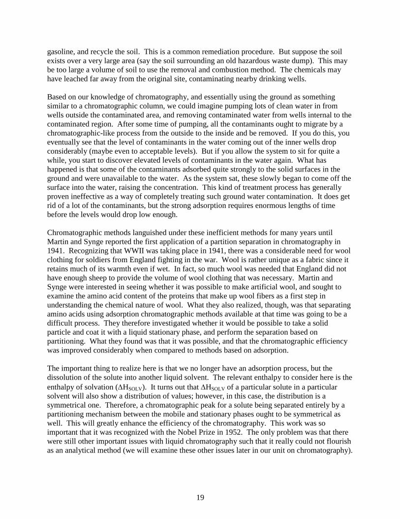
The key question for us to ask is what a chromatographic peak would look like for a solute

traveling through this stationary phase. Hopefully it seems reasonable to predict that the peak for

the solute would also be asymmetric. Those solute molecules adsorbed at the highly active sites

would essentially get stuck on the column and take much longer to elute. The asymmetric peak

observed in Figure 17 exhibits tailing. Note that tailed peaks are undesirable in chromatographic

separations because they are more likely to overlap with each other and interfere with the

separation. Unless the solid surface is highly deactivated, all chromatographic separations based

on adsorption will exhibit peak tailing. This causes an inherent inefficiency in adsorption

methods.

Figure 17. Tailed peak shape in adsorption chromatography

One last thing before we move on is to understand that strong adsorption by molecules on active

solid surfaces has a profound implication in environmental chemistry. Consider a leaking,

underground tank of gasoline at a service station. The soil around the tank gets contaminated by

the leaking gas and it is desirable to clean it up. One way is to remove all the contaminated soil,

heat it in a very high temperature oven that combusts all the hydrocarbon components of the

Frequency of

Occurrence

Low

Energy

High

Energy ΔHADS

Silanol

Overall

Disilanol

Trisilanol

INJ

19

gasoline, and recycle the soil. This is a common remediation procedure. But suppose the soil

exists over a very large area (say the soil surrounding an old hazardous waste dump). This may

be too large a volume of soil to use the removal and combustion method. The chemicals may

have leached far away from the original site, contaminating nearby drinking wells.

Based on our knowledge of chromatography, and essentially using the ground as something

similar to a chromatographic column, we could imagine pumping lots of clean water in from

wells outside the contaminated area, and removing contaminated water from wells internal to the

contaminated region. After some time of pumping, all the contaminants ought to migrate by a

chromatographic-like process from the outside to the inside and be removed. If you do this, you

eventually see that the level of contaminants in the water coming out of the inner wells drop

considerably (maybe even to acceptable levels). But if you allow the system to sit for quite a

while, you start to discover elevated levels of contaminants in the water again. What has

happened is that some of the contaminants adsorbed quite strongly to the solid surfaces in the

ground and were unavailable to the water. As the system sat, these slowly began to come off the

surface into the water, raising the concentration. This kind of treatment process has generally

proven ineffective as a way of completely treating such ground water contamination. It does get

rid of a lot of the contaminants, but the strong adsorption requires enormous lengths of time

before the levels would drop low enough.

Chromatographic methods languished under these inefficient methods for many years until

Martin and Synge reported the first application of a partition separation in chromatography in

1941. Recognizing that WWII was taking place in 1941, there was a considerable need for wool

clothing for soldiers from England fighting in the war. Wool is rather unique as a fabric since it

retains much of its warmth even if wet. In fact, so much wool was needed that England did not

have enough sheep to provide the volume of wool clothing that was necessary. Martin and

Synge were interested in seeing whether it was possible to make artificial wool, and sought to

examine the amino acid content of the proteins that make up wool fibers as a first step in

understanding the chemical nature of wool. What they also realized, though, was that separating

amino acids using adsorption chromatographic methods available at that time was going to be a

difficult process. They therefore investigated whether it would be possible to take a solid

particle and coat it with a liquid stationary phase, and perform the separation based on

partitioning. What they found was that it was possible, and that the chromatographic efficiency

was improved considerably when compared to methods based on adsorption.

The important thing to realize here is that we no longer have an adsorption process, but the

dissolution of the solute into another liquid solvent. The relevant enthalpy to consider here is the

enthalpy of solvation (HSOLV). It turns out that HSOLV of a particular solute in a particular

solvent will also show a distribution of values; however, in this case, the distribution is a

symmetrical one. Therefore, a chromatographic peak for a solute being separated entirely by a

partitioning mechanism between the mobile and stationary phases ought to be symmetrical as

well. This will greatly enhance the efficiency of the chromatography. This work was so

important that it was recognized with the Nobel Prize in 1952. The only problem was that there

were still other important issues with liquid chromatography such that it really could not flourish

as an analytical method (we will examine these other issues later in our unit on chromatography).

20

One intriguing aspect of Martin and Synge’s 1941 paper is the last sentence, which predicted that

it should be possible to use gas as the mobile phase (i.e., gas chromatography), and that some of

the limitations that restrict the efficiency of liquid chromatography should not occur in gas

chromatography. What was also interesting is that it was not until 1951, that James and Martin

published the first report in which gas chromatography was described as an analysis method.

Much of the delay was because of WWII and the need for scientists to devote their research to

areas of immediate national concern related to the war effort.

The introduction of gas chromatography revolutionized the entire field of chemical analysis.

One thing, as we will develop in the next substantial portion of this unit, is that gas

chromatographic methods had certain fundamental advantages over liquid chromatographic

methods when it came to column efficiency. It was possible, using gas chromatography, to

separate very complex mixtures of volatile chemicals in very short periods of time. Before gas

chromatography, no one even considered that it might be possible to separate as many as 50 to

100 constituents of a sample in only an hour. The other thing that prompted an explosion of

interest in gas chromatography as an analysis method was the development of some highly

sensitive methods of detection in the 1950s and 1960s. People were now able to sense levels of

molecules that were not detectable in other, conventional solution-phase systems. Part of the

problem with solution-phase analysis is the overwhelming volume of solvent that can interfere

with the technique used to perform the measurement. Gas phase measurements, where the

overall density of molecules is very low, do not have as much potential for interference from

gases other than those being measured.

What we now need to do is develop an understanding of what created the inherent advantage in

efficiency of gas chromatographic columns, and then understand what took place to improve the

efficiency of liquid chromatographic columns. When we talk about the efficiency of a

chromatographic column, what we really refer to is the width of the chromatographic bands of

solutes as they migrate through the column.

21

BROADENING OF CHROMATOGRAPHIC PEAKS

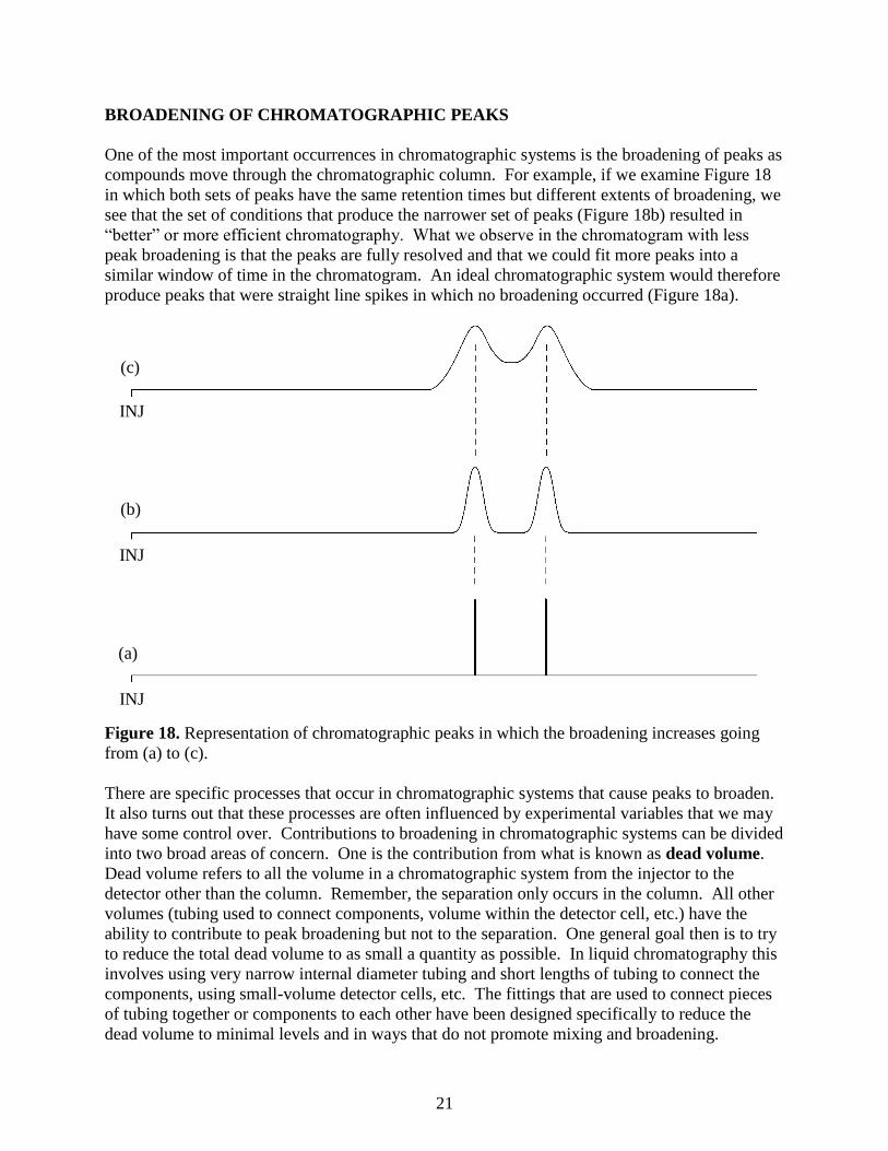
One of the most important occurrences in chromatographic systems is the broadening of peaks as

compounds move through the chromatographic column. For example, if we examine Figure 18

in which both sets of peaks have the same retention times but different extents of broadening, we

see that the set of conditions that produce the narrower set of peaks (Figure 18b) resulted in

“better” or more efficient chromatography. What we observe in the chromatogram with less

peak broadening is that the peaks are fully resolved and that we could fit more peaks into a

similar window of time in the chromatogram. An ideal chromatographic system would therefore

produce peaks that were straight line spikes in which no broadening occurred (Figure 18a).

Figure 18. Representation of chromatographic peaks in which the broadening increases going

from (a) to (c).

There are specific processes that occur in chromatographic systems that cause peaks to broaden.

It also turns out that these processes are often influenced by experimental variables that we may

have some control over. Contributions to broadening in chromatographic systems can be divided

into two broad areas of concern. One is the contribution from what is known as dead volume.

Dead volume refers to all the volume in a chromatographic system from the injector to the

detector other than the column. Remember, the separation only occurs in the column. All other

volumes (tubing used to connect components, volume within the detector cell, etc.) have the

ability to contribute to peak broadening but not to the separation. One general goal then is to try

to reduce the total dead volume to as small a quantity as possible. In liquid chromatography this

involves using very narrow internal diameter tubing and short lengths of tubing to connect the

components, using small-volume detector cells, etc. The fittings that are used to connect pieces

of tubing together or components to each other have been designed specifically to reduce the

dead volume to minimal levels and in ways that do not promote mixing and broadening.

INJ

INJ

INJ

(c)

(b)

(a)

22

The other source of broadening is within the column. If you were to examine state-of-the-art

columns that are used today in gas and liquid chromatography, it turns out that there are several

features of their design that lead to significant reductions in peak broadening. In other words,

these columns represent the best we can do today to reduce the broadening of peaks, and

therefore represent the most efficient column technology. It is worth taking the time to

understand the various contributions to peak broadening that occur within the chromatographic

column and to examine the ways in which current gas and liquid chromatographic columns have

been designed to minimize these effects.

There are four general contributions to broadening within chromatographic columns. These are

known as:

longitudinal diffusion

eddy diffusion

mass transport broadening in the stationary phase

mass transport broadening in the mobile phase

Before moving on, it is worth remembering back to two fundamental criteria we talked about

with regards to chromatographic columns, the number of theoretical plates (N) and the reduced

plate height (h). Remember that a column with more plates, or better yet a column with a small

reduced plate height, was more efficient and provided better separations. We can therefore use

the reduced plate height as a determining measure of the efficiency of a chromatographic

column. The smaller the value of h, the more efficient the column. What we will develop as

we analyze the four contributions to broadening above is an equation, which was first known as

the van Deemter equation (J. J. van Deemter described the first treatment of this for

chromatographic systems in 1956), that relates these four terms to the reduced plate height.

23

Longitudinal Diffusion Broadening in Chromatography

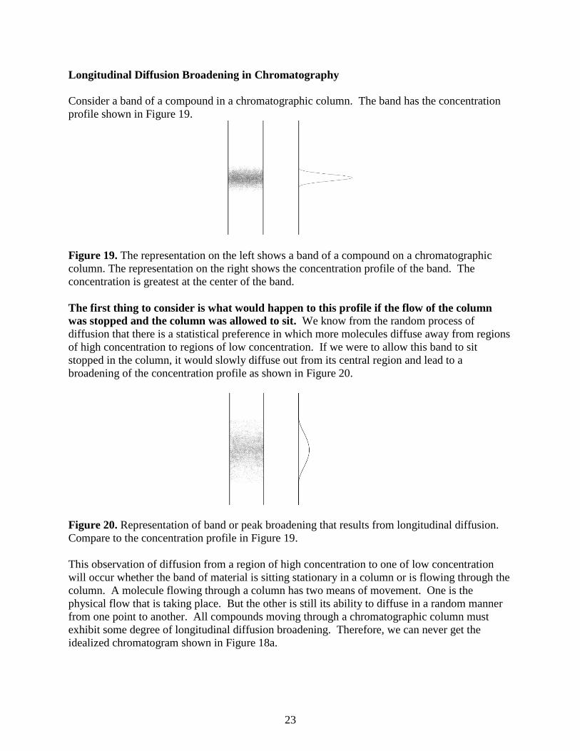
Consider a band of a compound in a chromatographic column. The band has the concentration

profile shown in Figure 19.

Figure 19. The representation on the left shows a band of a compound on a chromatographic

column. The representation on the right shows the concentration profile of the band. The

concentration is greatest at the center of the band.

The first thing to consider is what would happen to this profile if the flow of the column

was stopped and the column was allowed to sit. We know from the random process of

diffusion that there is a statistical preference in which more molecules diffuse away from regions

of high concentration to regions of low concentration. If we were to allow this band to sit

stopped in the column, it would slowly diffuse out from its central region and lead to a

broadening of the concentration profile as shown in Figure 20.

Figure 20. Representation of band or peak broadening that results from longitudinal diffusion.

Compare to the concentration profile in Figure 19.

This observation of diffusion from a region of high concentration to one of low concentration

will occur whether the band of material is sitting stationary in a column or is flowing through the

column. A molecule flowing through a column has two means of movement. One is the

physical flow that is taking place. But the other is still its ability to diffuse in a random manner

from one point to another. All compounds moving through a chromatographic column must

exhibit some degree of longitudinal diffusion broadening. Therefore, we can never get the

idealized chromatogram shown in Figure 18a.

24

An important thing to consider is whether this phenomenon is more significant (i.e.,

happens faster and therefore causes more broadening, everything else being equal) in gas

or liquid chromatography. To consider this, we would need to know something about the

relative rates of diffusion of gases and liquids. A substance with a faster rate of diffusion will

broaden more in a certain amount of time than something with a slower rate of diffusion. So the

relevant question is, which diffuses faster, gases or liquids? I suspect we all know that gases

diffuse appreciably faster than liquids. Just imagine yourself standing on the opposite side of a

room from someone who opens a bottle of a chemical with the odor of a skunk. How fast do you

smell this odor? Compare that with having the room full of water, and someone adds a drop of a

colored dye to the water at one side of the room. How fast would that color make its way across

the water to the other side of the room? In fact, gases have diffusion rates that are approximately

100,000 times faster than that of liquids. The potential contribution of longitudinal diffusion

broadening to chromatographic peaks is much more serious in gas chromatography than in liquid

chromatography. In liquid chromatography, the contribution of longitudinal diffusion

broadening is so low that it’s really never a significant contribution to peak broadening.

Finally, we could ask ourselves whether this phenomenon contributes more to band

broadening at higher or lower flow rates. What we need to recognize is that longitudinal

broadening occurs at some set rate that is only determined by the mobile phase (gas or liquid)

and the particular molecule undergoing diffusion. In the gas or liquid phase, it would be

reasonable to expect that a small molecule would have a faster rate of diffusion than a large

molecule. If we are doing conventional gas or liquid chromatography using organic compounds

with molecular weights from about 100 to 300, the differences in diffusion rates are not

sufficient enough to make large differences here. If we were comparing those molecules to

proteins with molecular weights of 50,000, there might be a significant difference in the rate of

diffusion in the liquid phase. If the longitudinal diffusion occurs at a set, fixed rate, then the

longer a compound (solute) is in the column, the more time it has to undergo longitudinal

diffusion. The compound would be in the column a longer time at a slower flow rate. This

allows us to say that the contribution of longitudinal diffusion to overall peak broadening will be

greater the slower the flow rate. If we use the term B to represent longitudinal diffusion

broadening and v to represent flow rate, and want to relate this to h, we would write the

following expression:

h = B

v

Remember that the smaller the reduced plate height the better. At high flow rates, B/v gets

smaller, h is smaller, and the contribution of longitudinal diffusion to peak broadening is smaller.

We can also write the following expression for B: B = 2DM

In this case, DM refers to the diffusivity (diffusion coefficient) of the solute in the solvent.

Notice that this is a direct relationship: the faster the rate of diffusion of the solute, the greater

the extent of longitudinal diffusion. is known as the obstruction factor, and occurs in a packed

chromatographic column. In solution, a molecule has an equal probability of diffusion in any

direction. In a packed column, the solid packing material may restrict the ability of the solute to

diffuse in a particular direction, thereby hindering longitudinal diffusion. This term takes this

effect into account.

25

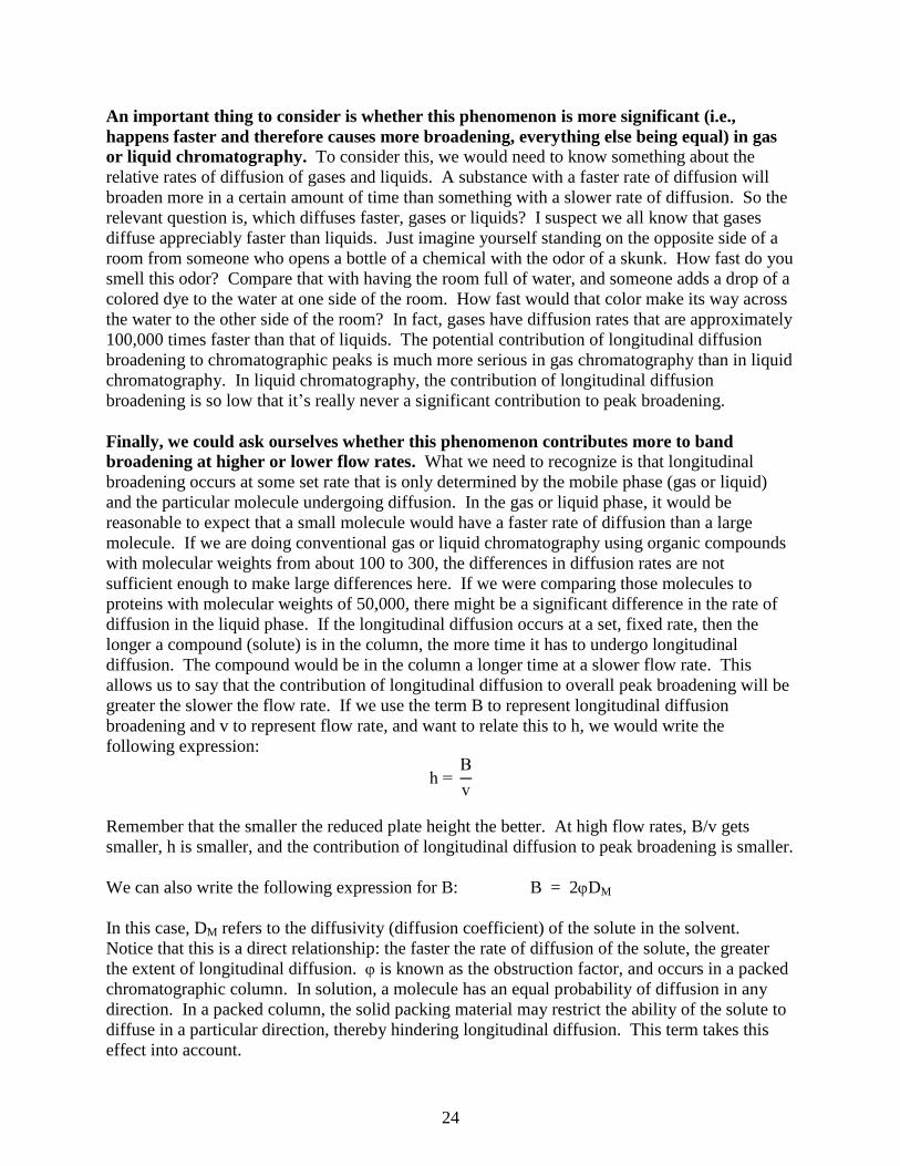
Eddy Diffusion (Multipath) Broadening in Chromatography

Consider a group of molecules flowing through a packed bed of particles (Figure 21). Another

way to think of this is to imagine you and a group of friends following a river downstream in a

set of inner tubes. The river has a number of rocks in the way and a variety of different flow

paths through the rocks. Different people go in different channels either because they paddle

over to them or get caught in different flows of the current as they bounce off of obstacles.

Figure 21. Representation of a chromatographic column packed with particles.

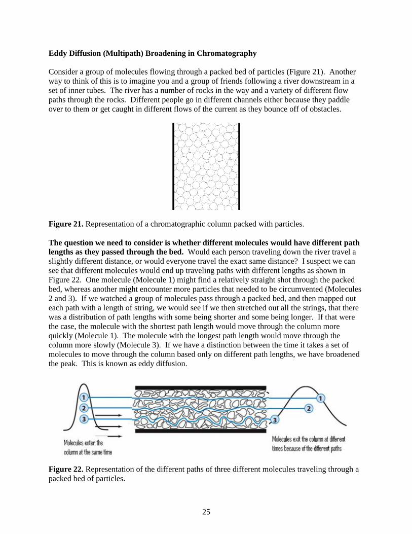
The question we need to consider is whether different molecules would have different path

lengths as they passed through the bed. Would each person traveling down the river travel a

slightly different distance, or would everyone travel the exact same distance? I suspect we can

see that different molecules would end up traveling paths with different lengths as shown in

Figure 22. One molecule (Molecule 1) might find a relatively straight shot through the packed

bed, whereas another might encounter more particles that needed to be circumvented (Molecules

2 and 3). If we watched a group of molecules pass through a packed bed, and then mapped out

each path with a length of string, we would see if we then stretched out all the strings, that there

was a distribution of path lengths with some being shorter and some being longer. If that were

the case, the molecule with the shortest path length would move through the column more

quickly (Molecule 1). The molecule with the longest path length would move through the

column more slowly (Molecule 3). If we have a distinction between the time it takes a set of

molecules to move through the column based only on different path lengths, we have broadened

the peak. This is known as eddy diffusion.

Figure 22. Representation of the different paths of three different molecules traveling through a

packed bed of particles.

26

A key factor to consider when examining eddy diffusion is to ask whether the difference in

length between the shortest and longest path depends at all on the diameter of the particles.

If it is, we could then ask which particles (smaller or larger) would lead to a greater difference in

path length?

Almost everyone who is asked the first question seems to intuitively realize that the size of the

particles must somehow make a difference. It just seems too coincidental to think that the

difference between the shortest and longest path would be identical if the particle sizes are

different. But interestingly enough, almost everyone, when they first consider this, seems to

select the wrong answer when figuring out which particle (small or large) would lead to a greater

difference in path length between the shortest and longest path. Remember, the important

distinction is the size of the difference between the shortest and longest path, not whether one

column would uniformly have longer path lengths than the other.

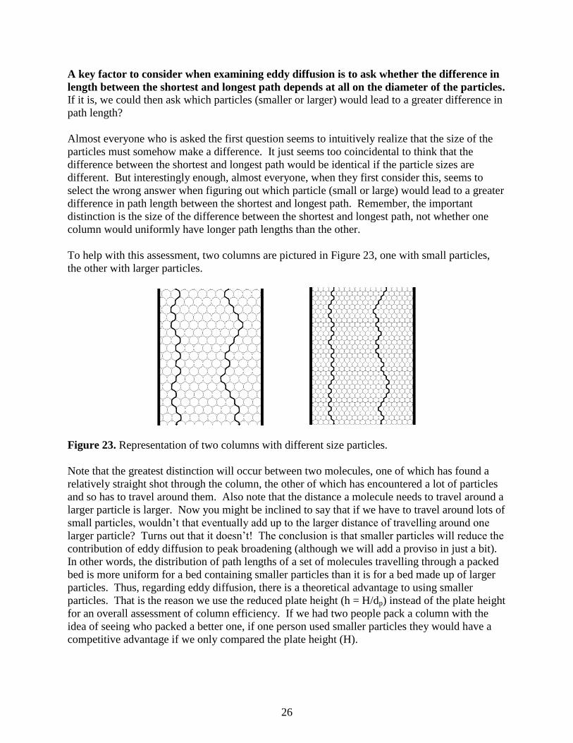
To help with this assessment, two columns are pictured in Figure 23, one with small particles,

the other with larger particles.

Figure 23. Representation of two columns with different size particles.

Note that the greatest distinction will occur between two molecules, one of which has found a

relatively straight shot through the column, the other of which has encountered a lot of particles

and so has to travel around them. Also note that the distance a molecule needs to travel around a

larger particle is larger. Now you might be inclined to say that if we have to travel around lots of

small particles, wouldn’t that eventually add up to the larger distance of travelling around one

larger particle? Turns out that it doesn’t! The conclusion is that smaller particles will reduce the

contribution of eddy diffusion to peak broadening (although we will add a proviso in just a bit).

In other words, the distribution of path lengths of a set of molecules travelling through a packed

bed is more uniform for a bed containing smaller particles than it is for a bed made up of larger

particles. Thus, regarding eddy diffusion, there is a theoretical advantage to using smaller

particles. That is the reason we use the reduced plate height (h = H/dp) instead of the plate height

for an overall assessment of column efficiency. If we had two people pack a column with the

idea of seeing who packed a better one, if one person used smaller particles they would have a

competitive advantage if we only compared the plate height (H).

27

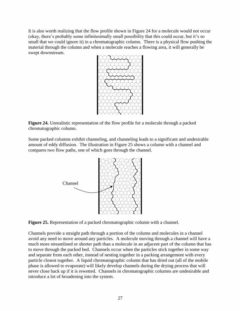
It is also worth realizing that the flow profile shown in Figure 24 for a molecule would not occur

(okay, there’s probably some infinitesimally small possibility that this could occur, but it’s so

small that we could ignore it) in a chromatographic column. There is a physical flow pushing the

material through the column and when a molecule reaches a flowing area, it will generally be

swept downstream.

Figure 24. Unrealistic representation of the flow profile for a molecule through a packed

chromatographic column.

Some packed columns exhibit channeling, and channeling leads to a significant and undesirable

amount of eddy diffusion. The illustration in Figure 25 shows a column with a channel and

compares two flow paths, one of which goes through the channel.

Figure 25. Representation of a packed chromatographic column with a channel.

Channels provide a straight path through a portion of the column and molecules in a channel

avoid any need to move around any particles. A molecule moving through a channel will have a

much more streamlined or shorter path than a molecule in an adjacent part of the column that has

to move through the packed bed. Channels occur when the particles stick together in some way

and separate from each other, instead of nesting together in a packing arrangement with every

particle closest together. A liquid chromatographic column that has dried out (all of the mobile

phase is allowed to evaporate) will likely develop channels during the drying process that will

never close back up if it is rewetted. Channels in chromatographic columns are undesirable and

introduce a lot of broadening into the system.

Channel

28

Another key thing to ask then is whether channeling is more likely to occur with smaller or

larger particles. Channeling will occur if a column is poorly packed. There are very specific

procedures that have been developed for packing gas and liquid chromatographic columns that

are designed to minimize the chance that channeling will occur. One key to packing a good

column is to slowly lay down a bed of particles so that they nest into each other as well as

possible. In packing a gas chromatographic column, this will usually involve slowly adding the

particles to the column while vibrating it so that the particles settle in together. Liquid

chromatographic columns are usually packed slowly under high pressure. A column is packed

efficiently when the particles are in a uniform bed with the minimum amount of voids. Given a

particular particle size, the goal is to fit as many of them as possible into the column. We can

then ask which is more difficult to pack efficiently, larger or smaller particles.

One way to think about this is if you were asked to fill a large box (say a refrigerator box) with

basketballs or tennis balls. The goal is to fit as many of either one in as possible. You could

imagine readily taking the time to carefully lay down each basketball into the refrigerator box,

layer by layer, and fitting in as many basketballs as possible. You might also be able to imagine

that you would start slowly with the tennis balls, laying in one in a time, and quickly lose

patience at how long this would take to fill the entire box. If you then sped up, say by slowing

dumping in balls from a pail while a helper shook the box, you would probably create more

voids in the box. Also, because the interstitial volumes between the tennis balls will be smaller

than that with the basketballs, any channels become more significant. The result is that it is more

difficult to avoid the formation of channels with smaller particles. Recapping, smaller particles

have a theoretical advantage over larger particles, but more care must be exercised when packing

smaller particles if this theoretical advantage in column efficiency is to be realized.

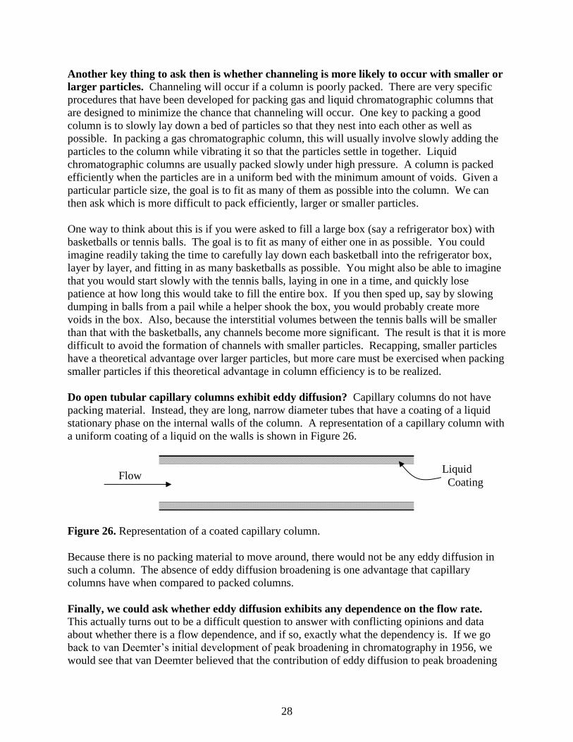
Do open tubular capillary columns exhibit eddy diffusion? Capillary columns do not have

packing material. Instead, they are long, narrow diameter tubes that have a coating of a liquid

stationary phase on the internal walls of the column. A representation of a capillary column with

a uniform coating of a liquid on the walls is shown in Figure 26.

Figure 26. Representation of a coated capillary column.

Because there is no packing material to move around, there would not be any eddy diffusion in

such a column. The absence of eddy diffusion broadening is one advantage that capillary

columns have when compared to packed columns.

Finally, we could ask whether eddy diffusion exhibits any dependence on the flow rate. This actually turns out to be a difficult question to answer with conflicting opinions and data

about whether there is a flow dependence, and if so, exactly what the dependency is. If we go

back to van Deemter’s initial development of peak broadening in chromatography in 1956, we

would see that van Deemter believed that the contribution of eddy diffusion to peak broadening

Flow Liquid

Coating

29

did not depend in any way on the flow rate. This is a reasonable argument if we thought that we

could draw a variety of different flow paths through a packed bed, and the difference in length

between the shortest and longest flow path would be fixed irrespective of how fast the molecules

were moving through the path.

But let’s return to our river analogy to see how the flow rate might get involved in this. Suppose

the river had a relatively fast flow rate, such that different people in different inner tubes got

locked into particular flow channels and stayed in those all the way down the river. Under that

situation, each path would have a preset length and even if we slowed down the flow, so long as

you were locked into a particular path, the difference in distance would be invariant. But

suppose now we slowed down the flow so much that there were opportunities to drift around at

points and sample a variety of flow paths down the river. This might lead to some averaging and

the amount of sampling of different flow paths would be greater the slower the flow. This same

thing can happen in a chromatographic column and leads to conflicting data and opinions about

the nature of any flow rate dependence on eddy diffusion. Also, the exact point at which there is

a crossover between a rapid flow that locks in a flow path versus a slow one that allows each

molecule to sample many different flow paths is impossible to determine. This point is still not

fully resolved, and literature on band broadening show different terms for eddy diffusion. We

usually denote eddy diffusion by the term A. If you look at van Deemter’s initial treatment of

peak broadening, you would see (note, van Deemter also did not use the reduced plate height, but

we could write h = A as well):

H = A

(where A = 2dp)

Note how the particle diameter (dp) is included in this equation for A, so that the smaller the

particle diameter, the smaller the contribution of eddy diffusion to the reduced plate height.

Another common conclusion today is that the contribution of eddy diffusion broadening does

exhibit a slight dependence on flow rate. The usual form of this is that the dependence is v1/3

,

and you might often see books or articles that include the following term in the overall band

broadening equation.

h = A v1/3

Still other people throw up their hands at all the confusion regarding eddy diffusion and show

overall band broadening equations that do not have any A-term in them. We will develop

another broadening term that has to do with processes going on in the mobile phase (and note

that eddy diffusion only involves the mobile phase - none of what we talked about even requires

the presence of a liquid stationary phase), so some people lump the eddy diffusion term into this

other mobile phase term.

30

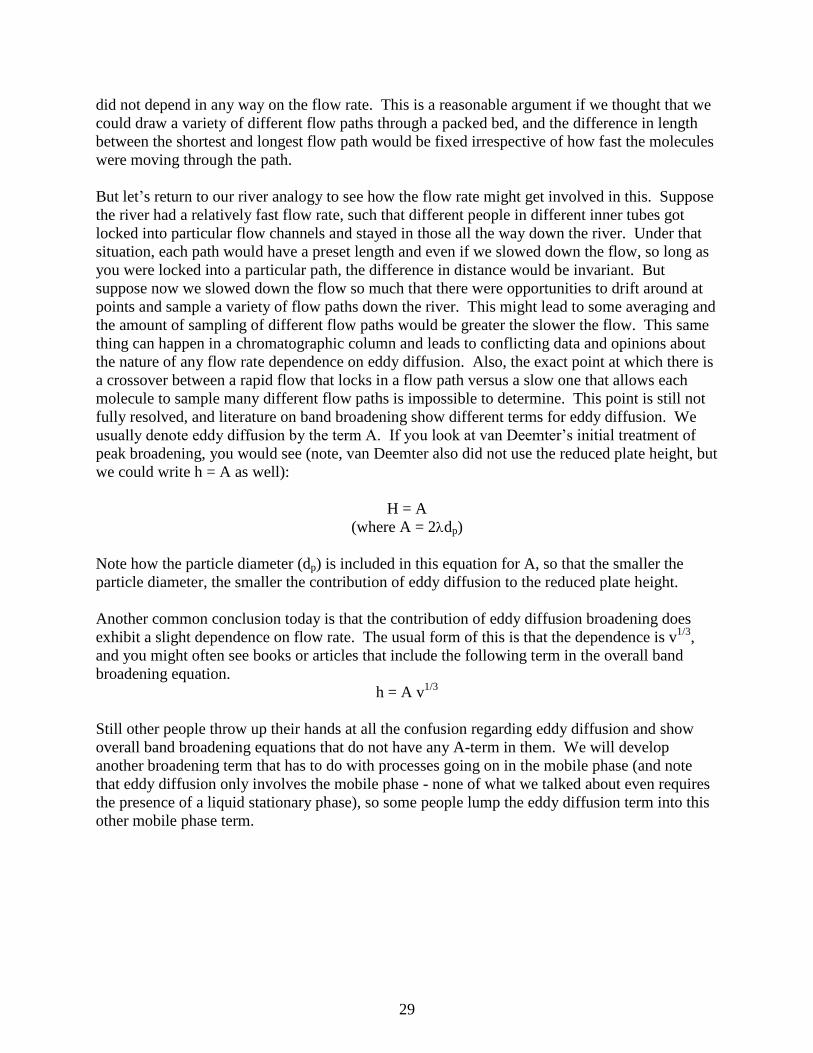
Stationary Phase Mass Transport Broadening

Consider a compound that has distributed between the mobile and stationary phase within a plate

in a chromatographic column. Figure 27 might represent the concentration distribution profiles

in the two phases (note that the compound, as depicted, has a slight preference for the mobile

phase).

Figure 27. Representation of the concentration profiles for a compound distributed between the

stationary (left) and mobile (right) phases of a chromatographic column. Note that the

compound has a preference for the mobile phase.

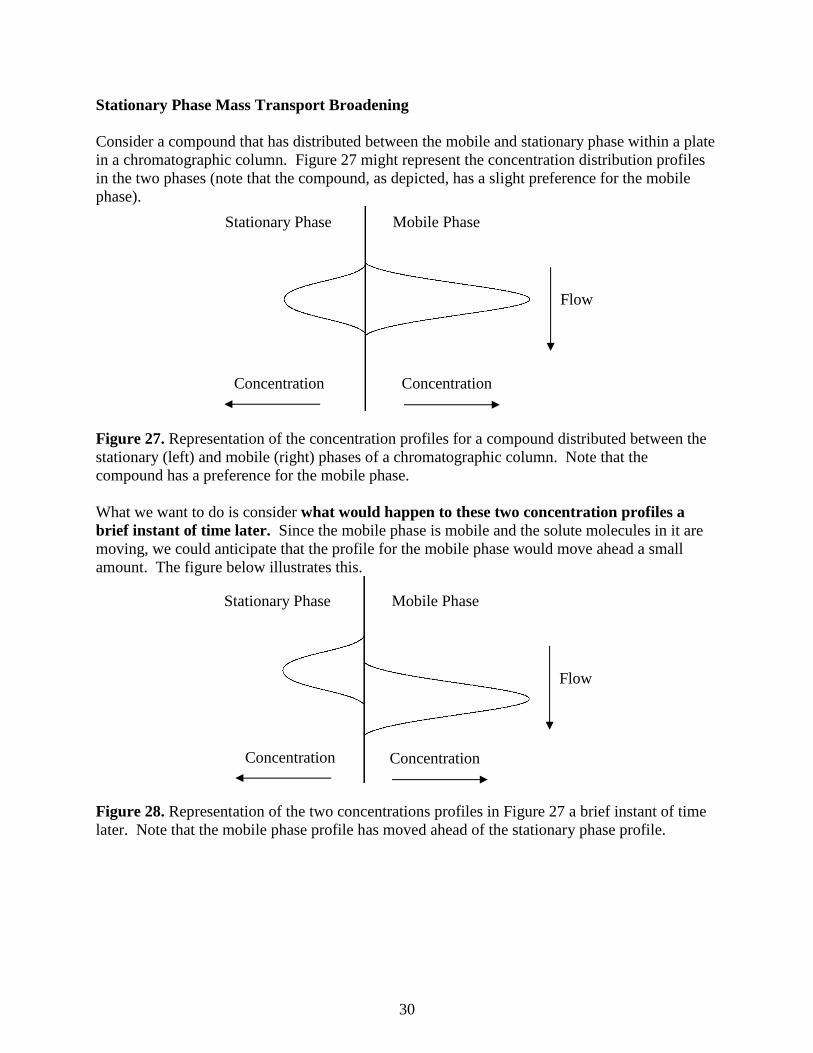
What we want to do is consider what would happen to these two concentration profiles a

brief instant of time later. Since the mobile phase is mobile and the solute molecules in it are

moving, we could anticipate that the profile for the mobile phase would move ahead a small

amount. The figure below illustrates this.

Figure 28. Representation of the two concentrations profiles in Figure 27 a brief instant of time

later. Note that the mobile phase profile has moved ahead of the stationary phase profile.

Stationary Phase Mobile Phase

Concentration Concentration

Flow

Stationary Phase Mobile Phase

Concentration Concentration

Flow

31

What about the concentration profile for the solute molecules in the stationary phase? Consider

the picture in Figure 29 for two solute molecules dissolved in the stationary phase of a capillary

column and let’s assume that these are at the trailing edge of the stationary phase distribution.

Figure 29. Two molecules dissolved in the liquid stationary phase of a capillary column.

What we observe is that the molecule labeled 1 is right at the interface between the stationary

and mobile phase and provided it is diffusing in the right direction, it can transfer out into the

mobile phase and move along. The molecule labeled 2, however, is “trapped” in the stationary

phase. It cannot get out into the mobile phase until it first diffuses up to the interface. We refer

to this process as mass transport. The solute molecules in the stationary phase must be

transported up to the interface before they can switch phases. What we observe is that the solute

molecules must spend a finite amount of time in the stationary phase. Since the mobile phase

solute molecules are moving away, molecules stuck in the stationary phase lag behind and

introduce a degree of broadening.

If we then consider the leading edge of the mobile phase distribution, we would observe that the

molecules are encountering fresh stationary phase with no dissolved solute molecules and so

these start to diffuse into the stationary phase when they encounter the surface. We can illustrate

this in Figure 30 with arrows showing the direction of migration of solute molecules out of the

stationary phase at the trailing edge and into the stationary phase at the leading edge.

Figure 30. Representation of the movement of analyte molecules at the leading and trailing edge

of the concentration distribution.

Hopefully it is obvious from Figure 30 that the finite time required for the molecules to move out

of the stationary phase leads to an overall broadening of the concentration distribution and

overall broadening of the peak.

#1 #2

Liquid Coating

Stationary Phase Mobile Phase

Concentration Concentration

Flow

32

A critical question to ask is whether the contribution of stationary phase mass transport

broadening exhibits a dependence on the flow rate. Suppose we go back to the small amount

of time in the first part above, but now double the flow rate. Comparing the first situation (solid

line in the figure above) to that with double the flow rate (dashed line) leads to the two profiles.

Hopefully it is apparent that the higher flow rate leads to a greater discrepancy between the

mobile and stationary phase concentration distributions, which would lead to more broadening.

The term used to express mass transport broadening in the stationary phase is CS (not to be

confused with the CS that we have been using earlier to denote the concentration of solute in the

stationary phase). If we wanted to incorporate this into our overall band broadening equation,

recognizing that higher flow rates lead to more mass transport broadening and reduced column

efficiency (higher values of h), it would take the following form:

h = CS v

Something we might ask is whether the flow rate dependency of the stationary phase mass

transport term has any troublesome aspects. An alternative way to phrase this question is to

ask whether we would like to use slow or fast flow rates when performing chromatographic

separations. The advantage of fast flow rates is that the chromatographic separation will take

place in a shorter time. Since “time is money”, shorter analysis times are preferred (unless you

like to read long novels, and so prefer to inject a sample and then have an hour of reading time

while the compounds wend their way through the column). If you work for Wenzel Analytical,

we’re going to try to perform analyses as fast as possible and maximize our throughput. The

problem with speeding up the flow rate too high is that we begin to introduce large amounts of

stationary phase mass transport broadening. The shortening of the analysis time begins to be

offset by broad peaks that are not fully separated. Ultimately, stationary phase mass transport

broadening forces us to make a compromise between adequate efficiency and analysis time. You

cannot optimize both at the same time.

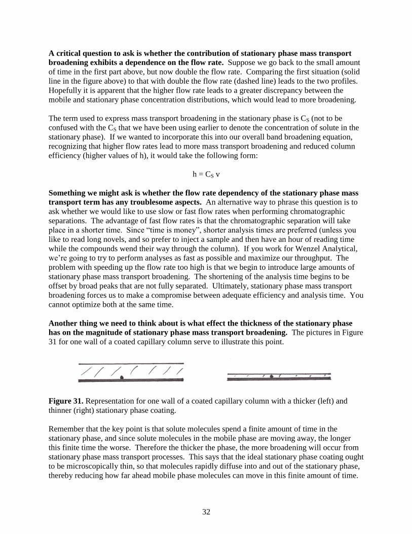
Another thing we need to think about is what effect the thickness of the stationary phase

has on the magnitude of stationary phase mass transport broadening. The pictures in Figure

31 for one wall of a coated capillary column serve to illustrate this point.

Figure 31. Representation for one wall of a coated capillary column with a thicker (left) and

thinner (right) stationary phase coating.

Remember that the key point is that solute molecules spend a finite amount of time in the

stationary phase, and since solute molecules in the mobile phase are moving away, the longer

this finite time the worse. Therefore the thicker the phase, the more broadening will occur from

stationary phase mass transport processes. This says that the ideal stationary phase coating ought

to be microscopically thin, so that molecules rapidly diffuse into and out of the stationary phase,

thereby reducing how far ahead mobile phase molecules can move in this finite amount of time.

33

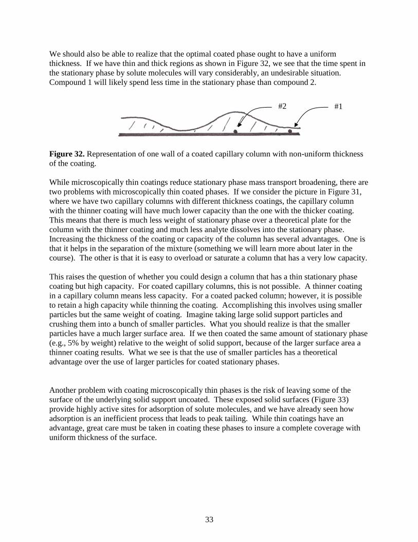
We should also be able to realize that the optimal coated phase ought to have a uniform

thickness. If we have thin and thick regions as shown in Figure 32, we see that the time spent in

the stationary phase by solute molecules will vary considerably, an undesirable situation.

Compound 1 will likely spend less time in the stationary phase than compound 2.

Figure 32. Representation of one wall of a coated capillary column with non-uniform thickness

of the coating.

While microscopically thin coatings reduce stationary phase mass transport broadening, there are

two problems with microscopically thin coated phases. If we consider the picture in Figure 31,

where we have two capillary columns with different thickness coatings, the capillary column

with the thinner coating will have much lower capacity than the one with the thicker coating.

This means that there is much less weight of stationary phase over a theoretical plate for the

column with the thinner coating and much less analyte dissolves into the stationary phase.

Increasing the thickness of the coating or capacity of the column has several advantages. One is

that it helps in the separation of the mixture (something we will learn more about later in the

course). The other is that it is easy to overload or saturate a column that has a very low capacity.

This raises the question of whether you could design a column that has a thin stationary phase

coating but high capacity. For coated capillary columns, this is not possible. A thinner coating

in a capillary column means less capacity. For a coated packed column; however, it is possible

to retain a high capacity while thinning the coating. Accomplishing this involves using smaller

particles but the same weight of coating. Imagine taking large solid support particles and

crushing them into a bunch of smaller particles. What you should realize is that the smaller

particles have a much larger surface area. If we then coated the same amount of stationary phase

(e.g., 5% by weight) relative to the weight of solid support, because of the larger surface area a

thinner coating results. What we see is that the use of smaller particles has a theoretical

advantage over the use of larger particles for coated stationary phases.

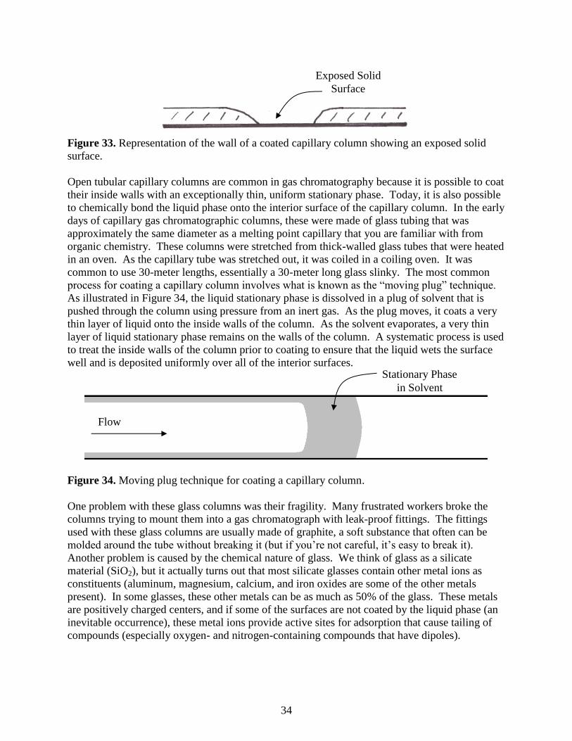
Another problem with coating microscopically thin phases is the risk of leaving some of the

surface of the underlying solid support uncoated. These exposed solid surfaces (Figure 33)

provide highly active sites for adsorption of solute molecules, and we have already seen how

adsorption is an inefficient process that leads to peak tailing. While thin coatings have an

advantage, great care must be taken in coating these phases to insure a complete coverage with

uniform thickness of the surface.

#1 #2

34

Figure 33. Representation of the wall of a coated capillary column showing an exposed solid

surface.

Open tubular capillary columns are common in gas chromatography because it is possible to coat

their inside walls with an exceptionally thin, uniform stationary phase. Today, it is also possible

to chemically bond the liquid phase onto the interior surface of the capillary column. In the early

days of capillary gas chromatographic columns, these were made of glass tubing that was

approximately the same diameter as a melting point capillary that you are familiar with from

organic chemistry. These columns were stretched from thick-walled glass tubes that were heated

in an oven. As the capillary tube was stretched out, it was coiled in a coiling oven. It was

common to use 30-meter lengths, essentially a 30-meter long glass slinky. The most common

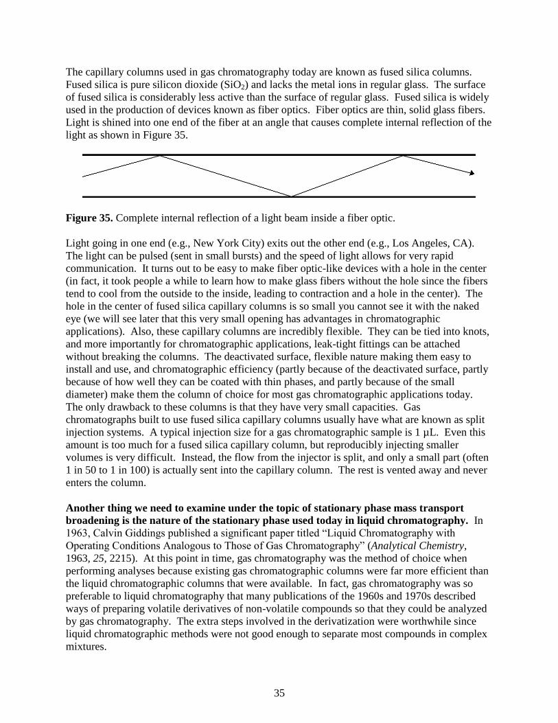
process for coating a capillary column involves what is known as the “moving plug” technique.

As illustrated in Figure 34, the liquid stationary phase is dissolved in a plug of solvent that is

pushed through the column using pressure from an inert gas. As the plug moves, it coats a very

thin layer of liquid onto the inside walls of the column. As the solvent evaporates, a very thin

layer of liquid stationary phase remains on the walls of the column. A systematic process is used

to treat the inside walls of the column prior to coating to ensure that the liquid wets the surface

well and is deposited uniformly over all of the interior surfaces.

Figure 34. Moving plug technique for coating a capillary column.

One problem with these glass columns was their fragility. Many frustrated workers broke the

columns trying to mount them into a gas chromatograph with leak-proof fittings. The fittings

used with these glass columns are usually made of graphite, a soft substance that often can be

molded around the tube without breaking it (but if you’re not careful, it’s easy to break it).

Another problem is caused by the chemical nature of glass. We think of glass as a silicate

material (SiO2), but it actually turns out that most silicate glasses contain other metal ions as

constituents (aluminum, magnesium, calcium, and iron oxides are some of the other metals

present). In some glasses, these other metals can be as much as 50% of the glass. These metals

are positively charged centers, and if some of the surfaces are not coated by the liquid phase (an

inevitable occurrence), these metal ions provide active sites for adsorption that cause tailing of

compounds (especially oxygen- and nitrogen-containing compounds that have dipoles).

Exposed Solid

Surface

Flow

Stationary Phase

in Solvent

35

The capillary columns used in gas chromatography today are known as fused silica columns.

Fused silica is pure silicon dioxide (SiO2) and lacks the metal ions in regular glass. The surface

of fused silica is considerably less active than the surface of regular glass. Fused silica is widely

used in the production of devices known as fiber optics. Fiber optics are thin, solid glass fibers.

Light is shined into one end of the fiber at an angle that causes complete internal reflection of the

light as shown in Figure 35.

Figure 35. Complete internal reflection of a light beam inside a fiber optic.

Light going in one end (e.g., New York City) exits out the other end (e.g., Los Angeles, CA).

The light can be pulsed (sent in small bursts) and the speed of light allows for very rapid

communication. It turns out to be easy to make fiber optic-like devices with a hole in the center

(in fact, it took people a while to learn how to make glass fibers without the hole since the fibers

tend to cool from the outside to the inside, leading to contraction and a hole in the center). The

hole in the center of fused silica capillary columns is so small you cannot see it with the naked

eye (we will see later that this very small opening has advantages in chromatographic

applications). Also, these capillary columns are incredibly flexible. They can be tied into knots,

and more importantly for chromatographic applications, leak-tight fittings can be attached

without breaking the columns. The deactivated surface, flexible nature making them easy to

install and use, and chromatographic efficiency (partly because of the deactivated surface, partly

because of how well they can be coated with thin phases, and partly because of the small

diameter) make them the column of choice for most gas chromatographic applications today.

The only drawback to these columns is that they have very small capacities. Gas

chromatographs built to use fused silica capillary columns usually have what are known as split

injection systems. A typical injection size for a gas chromatographic sample is 1 µL. Even this

amount is too much for a fused silica capillary column, but reproducibly injecting smaller

volumes is very difficult. Instead, the flow from the injector is split, and only a small part (often

1 in 50 to 1 in 100) is actually sent into the capillary column. The rest is vented away and never

enters the column.

Another thing we need to examine under the topic of stationary phase mass transport

broadening is the nature of the stationary phase used today in liquid chromatography. In

1963, Calvin Giddings published a significant paper titled “Liquid Chromatography with

Operating Conditions Analogous to Those of Gas Chromatography” (Analytical Chemistry,

1963, 25, 2215). At this point in time, gas chromatography was the method of choice when

performing analyses because existing gas chromatographic columns were far more efficient than

the liquid chromatographic columns that were available. In fact, gas chromatography was so

preferable to liquid chromatography that many publications of the 1960s and 1970s described

ways of preparing volatile derivatives of non-volatile compounds so that they could be analyzed

by gas chromatography. The extra steps involved in the derivatization were worthwhile since

liquid chromatographic methods were not good enough to separate most compounds in complex

mixtures.

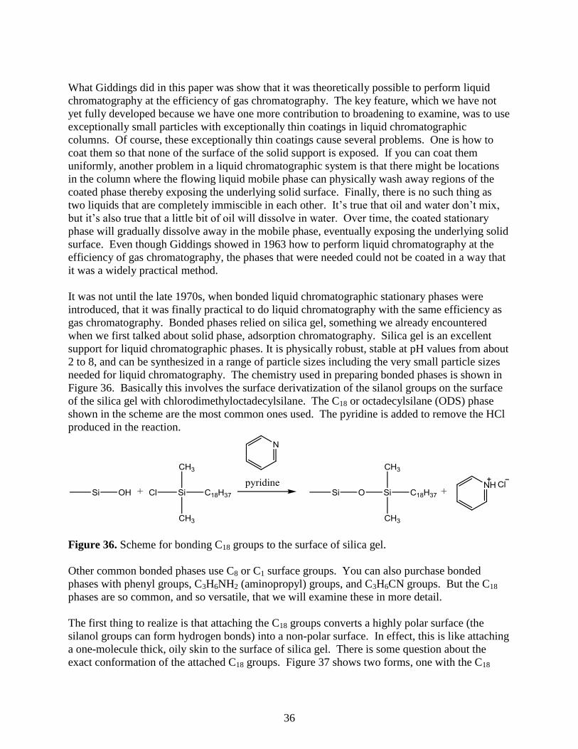
36

What Giddings did in this paper was show that it was theoretically possible to perform liquid

chromatography at the efficiency of gas chromatography. The key feature, which we have not

yet fully developed because we have one more contribution to broadening to examine, was to use

exceptionally small particles with exceptionally thin coatings in liquid chromatographic

columns. Of course, these exceptionally thin coatings cause several problems. One is how to

coat them so that none of the surface of the solid support is exposed. If you can coat them

uniformly, another problem in a liquid chromatographic system is that there might be locations

in the column where the flowing liquid mobile phase can physically wash away regions of the

coated phase thereby exposing the underlying solid surface. Finally, there is no such thing as

two liquids that are completely immiscible in each other. It’s true that oil and water don’t mix,

but it’s also true that a little bit of oil will dissolve in water. Over time, the coated stationary

phase will gradually dissolve away in the mobile phase, eventually exposing the underlying solid

surface. Even though Giddings showed in 1963 how to perform liquid chromatography at the

efficiency of gas chromatography, the phases that were needed could not be coated in a way that

it was a widely practical method.

It was not until the late 1970s, when bonded liquid chromatographic stationary phases were

introduced, that it was finally practical to do liquid chromatography with the same efficiency as

gas chromatography. Bonded phases relied on silica gel, something we already encountered

when we first talked about solid phase, adsorption chromatography. Silica gel is an excellent

support for liquid chromatographic phases. It is physically robust, stable at pH values from about

2 to 8, and can be synthesized in a range of particle sizes including the very small particle sizes

needed for liquid chromatography. The chemistry used in preparing bonded phases is shown in

Figure 36. Basically this involves the surface derivatization of the silanol groups on the surface

of the silica gel with chlorodimethyloctadecylsilane. The C18 or octadecylsilane (ODS) phase

shown in the scheme are the most common ones used. The pyridine is added to remove the HCl

produced in the reaction.

Figure 36. Scheme for bonding C18 groups to the surface of silica gel.

Other common bonded phases use C8 or C1 surface groups. You can also purchase bonded

phases with phenyl groups, C3H6NH2 (aminopropyl) groups, and C3H6CN groups. But the C18

phases are so common, and so versatile, that we will examine these in more detail.

The first thing to realize is that attaching the C18 groups converts a highly polar surface (the

silanol groups can form hydrogen bonds) into a non-polar surface. In effect, this is like attaching

a one-molecule thick, oily skin to the surface of silica gel. There is some question about the

exact conformation of the attached C18 groups. Figure 37 shows two forms, one with the C18

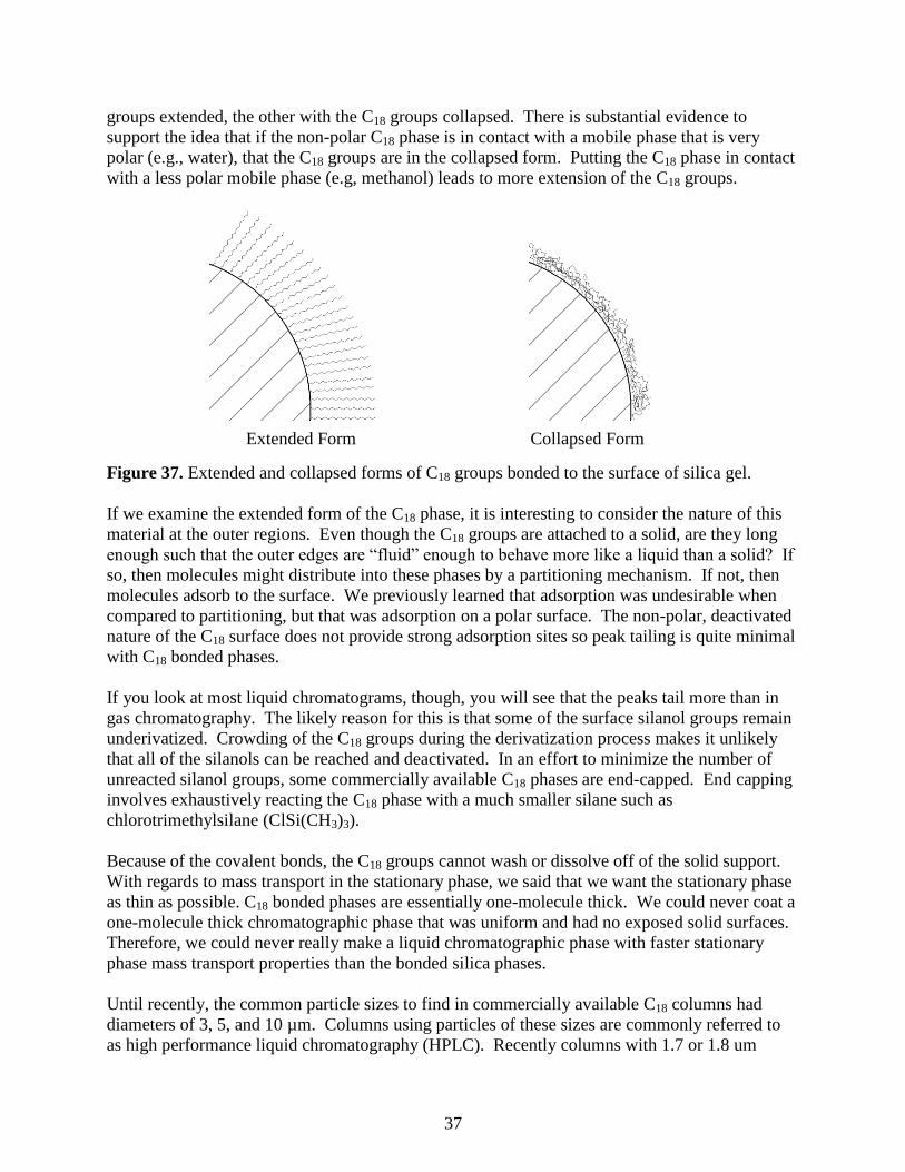
37

groups extended, the other with the C18 groups collapsed. There is substantial evidence to

support the idea that if the non-polar C18 phase is in contact with a mobile phase that is very

polar (e.g., water), that the C18 groups are in the collapsed form. Putting the C18 phase in contact

with a less polar mobile phase (e.g, methanol) leads to more extension of the C18 groups.

Figure 37. Extended and collapsed forms of C18 groups bonded to the surface of silica gel.

If we examine the extended form of the C18 phase, it is interesting to consider the nature of this

material at the outer regions. Even though the C18 groups are attached to a solid, are they long

enough such that the outer edges are “fluid” enough to behave more like a liquid than a solid? If

so, then molecules might distribute into these phases by a partitioning mechanism. If not, then

molecules adsorb to the surface. We previously learned that adsorption was undesirable when

compared to partitioning, but that was adsorption on a polar surface. The non-polar, deactivated

nature of the C18 surface does not provide strong adsorption sites so peak tailing is quite minimal

with C18 bonded phases.

If you look at most liquid chromatograms, though, you will see that the peaks tail more than in

gas chromatography. The likely reason for this is that some of the surface silanol groups remain

underivatized. Crowding of the C18 groups during the derivatization process makes it unlikely

that all of the silanols can be reached and deactivated. In an effort to minimize the number of

unreacted silanol groups, some commercially available C18 phases are end-capped. End capping

involves exhaustively reacting the C18 phase with a much smaller silane such as

chlorotrimethylsilane (ClSi(CH3)3).

Because of the covalent bonds, the C18 groups cannot wash or dissolve off of the solid support.

With regards to mass transport in the stationary phase, we said that we want the stationary phase

as thin as possible. C18 bonded phases are essentially one-molecule thick. We could never coat a

one-molecule thick chromatographic phase that was uniform and had no exposed solid surfaces.

Therefore, we could never really make a liquid chromatographic phase with faster stationary

phase mass transport properties than the bonded silica phases.

Until recently, the common particle sizes to find in commercially available C18 columns had

diameters of 3, 5, and 10 µm. Columns using particles of these sizes are commonly referred to

as high performance liquid chromatography (HPLC). Recently columns with 1.7 or 1.8 um

Extended Form Collapsed Form

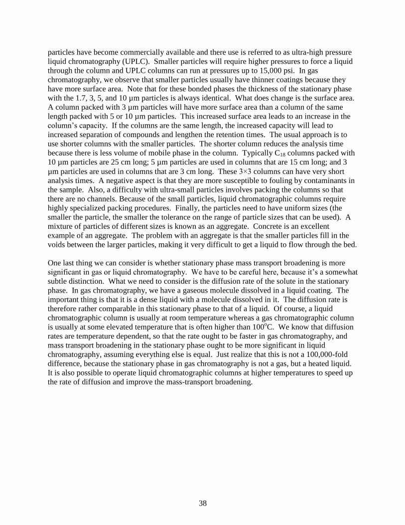
38

particles have become commercially available and there use is referred to as ultra-high pressure

liquid chromatography (UPLC). Smaller particles will require higher pressures to force a liquid

through the column and UPLC columns can run at pressures up to 15,000 psi. In gas

chromatography, we observe that smaller particles usually have thinner coatings because they

have more surface area. Note that for these bonded phases the thickness of the stationary phase

with the 1.7, 3, 5, and 10 µm particles is always identical. What does change is the surface area.

A column packed with 3 µm particles will have more surface area than a column of the same

length packed with 5 or 10 µm particles. This increased surface area leads to an increase in the

column’s capacity. If the columns are the same length, the increased capacity will lead to

increased separation of compounds and lengthen the retention times. The usual approach is to

use shorter columns with the smaller particles. The shorter column reduces the analysis time

because there is less volume of mobile phase in the column. Typically C18 columns packed with

10 µm particles are 25 cm long; 5 µm particles are used in columns that are 15 cm long; and 3

µm particles are used in columns that are 3 cm long. These 3×3 columns can have very short

analysis times. A negative aspect is that they are more susceptible to fouling by contaminants in

the sample. Also, a difficulty with ultra-small particles involves packing the columns so that

there are no channels. Because of the small particles, liquid chromatographic columns require

highly specialized packing procedures. Finally, the particles need to have uniform sizes (the

smaller the particle, the smaller the tolerance on the range of particle sizes that can be used). A

mixture of particles of different sizes is known as an aggregate. Concrete is an excellent

example of an aggregate. The problem with an aggregate is that the smaller particles fill in the

voids between the larger particles, making it very difficult to get a liquid to flow through the bed.

One last thing we can consider is whether stationary phase mass transport broadening is more

significant in gas or liquid chromatography. We have to be careful here, because it’s a somewhat

subtle distinction. What we need to consider is the diffusion rate of the solute in the stationary

phase. In gas chromatography, we have a gaseous molecule dissolved in a liquid coating. The

important thing is that it is a dense liquid with a molecule dissolved in it. The diffusion rate is

therefore rather comparable in this stationary phase to that of a liquid. Of course, a liquid

chromatographic column is usually at room temperature whereas a gas chromatographic column

is usually at some elevated temperature that is often higher than 100oC. We know that diffusion

rates are temperature dependent, so that the rate ought to be faster in gas chromatography, and

mass transport broadening in the stationary phase ought to be more significant in liquid

chromatography, assuming everything else is equal. Just realize that this is not a 100,000-fold

difference, because the stationary phase in gas chromatography is not a gas, but a heated liquid.

It is also possible to operate liquid chromatographic columns at higher temperatures to speed up

the rate of diffusion and improve the mass-transport broadening.

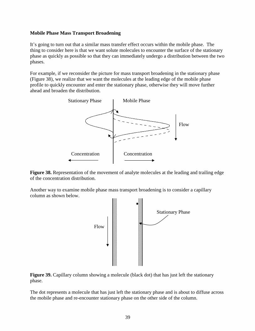
39

Mobile Phase Mass Transport Broadening

It’s going to turn out that a similar mass transfer effect occurs within the mobile phase. The

thing to consider here is that we want solute molecules to encounter the surface of the stationary

phase as quickly as possible so that they can immediately undergo a distribution between the two

phases.

For example, if we reconsider the picture for mass transport broadening in the stationary phase

(Figure 38), we realize that we want the molecules at the leading edge of the mobile phase

profile to quickly encounter and enter the stationary phase, otherwise they will move further

ahead and broaden the distribution.

Figure 38. Representation of the movement of analyte molecules at the leading and trailing edge

of the concentration distribution.

Another way to examine mobile phase mass transport broadening is to consider a capillary

column as shown below.

Figure 39. Capillary column showing a molecule (black dot) that has just left the stationary

phase.

The dot represents a molecule that has just left the stationary phase and is about to diffuse across

the mobile phase and re-encounter stationary phase on the other side of the column.

Stationary Phase Mobile Phase

Concentration Concentration

Flow

Stationary Phase

Flow

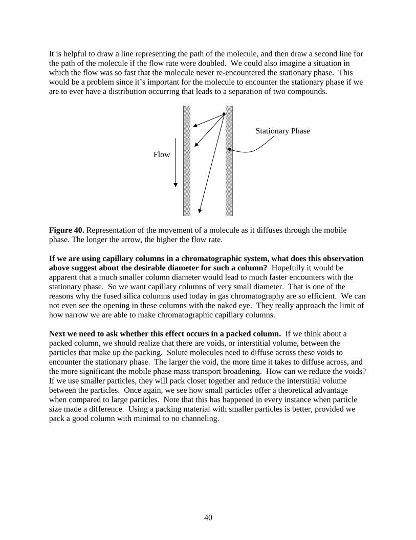
40

It is helpful to draw a line representing the path of the molecule, and then draw a second line for

the path of the molecule if the flow rate were doubled. We could also imagine a situation in

which the flow was so fast that the molecule never re-encountered the stationary phase. This

would be a problem since it’s important for the molecule to encounter the stationary phase if we

are to ever have a distribution occurring that leads to a separation of two compounds.

Figure 40. Representation of the movement of a molecule as it diffuses through the mobile

phase. The longer the arrow, the higher the flow rate.

If we are using capillary columns in a chromatographic system, what does this observation

above suggest about the desirable diameter for such a column? Hopefully it would be

apparent that a much smaller column diameter would lead to much faster encounters with the

stationary phase. So we want capillary columns of very small diameter. That is one of the

reasons why the fused silica columns used today in gas chromatography are so efficient. We can

not even see the opening in these columns with the naked eye. They really approach the limit of

how narrow we are able to make chromatographic capillary columns.

Next we need to ask whether this effect occurs in a packed column. If we think about a

packed column, we should realize that there are voids, or interstitial volume, between the

particles that make up the packing. Solute molecules need to diffuse across these voids to

encounter the stationary phase. The larger the void, the more time it takes to diffuse across, and

the more significant the mobile phase mass transport broadening. How can we reduce the voids?

If we use smaller particles, they will pack closer together and reduce the interstitial volume

between the particles. Once again, we see how small particles offer a theoretical advantage

when compared to large particles. Note that this has happened in every instance when particle

size made a difference. Using a packing material with smaller particles is better, provided we

pack a good column with minimal to no channeling.

Stationary Phase

Flow

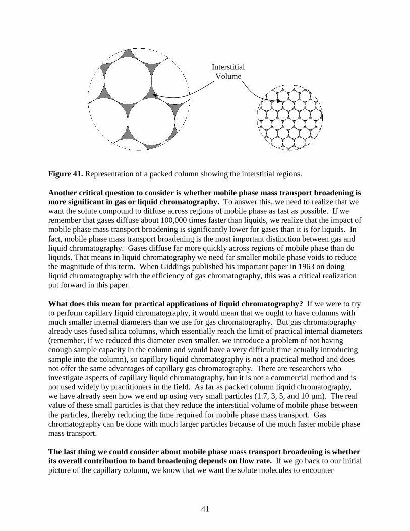
41

Figure 41. Representation of a packed column showing the interstitial regions.

Another critical question to consider is whether mobile phase mass transport broadening is

more significant in gas or liquid chromatography. To answer this, we need to realize that we

want the solute compound to diffuse across regions of mobile phase as fast as possible. If we

remember that gases diffuse about 100,000 times faster than liquids, we realize that the impact of

mobile phase mass transport broadening is significantly lower for gases than it is for liquids. In

fact, mobile phase mass transport broadening is the most important distinction between gas and

liquid chromatography. Gases diffuse far more quickly across regions of mobile phase than do

liquids. That means in liquid chromatography we need far smaller mobile phase voids to reduce

the magnitude of this term. When Giddings published his important paper in 1963 on doing

liquid chromatography with the efficiency of gas chromatography, this was a critical realization

put forward in this paper.

What does this mean for practical applications of liquid chromatography? If we were to try

to perform capillary liquid chromatography, it would mean that we ought to have columns with

much smaller internal diameters than we use for gas chromatography. But gas chromatography

already uses fused silica columns, which essentially reach the limit of practical internal diameters

(remember, if we reduced this diameter even smaller, we introduce a problem of not having

enough sample capacity in the column and would have a very difficult time actually introducing

sample into the column), so capillary liquid chromatography is not a practical method and does

not offer the same advantages of capillary gas chromatography. There are researchers who

investigate aspects of capillary liquid chromatography, but it is not a commercial method and is

not used widely by practitioners in the field. As far as packed column liquid chromatography,

we have already seen how we end up using very small particles (1.7, 3, 5, and 10 µm). The real

value of these small particles is that they reduce the interstitial volume of mobile phase between

the particles, thereby reducing the time required for mobile phase mass transport. Gas

chromatography can be done with much larger particles because of the much faster mobile phase

mass transport.

The last thing we could consider about mobile phase mass transport broadening is whether

its overall contribution to band broadening depends on flow rate. If we go back to our initial

picture of the capillary column, we know that we want the solute molecules to encounter

Interstitial

Volume

42

stationary phase as often as possible. The faster the flow, the fewer encounters, so a faster flow

makes this contribution worse (this is analogous to the leading edge of the mobile phase

distribution moving ahead more per unit time, thereby causing more broadening of the overall

distribution). If we needed to write a term to go into our equation for h, and we represent mobile

phase mass transport broadening as CM (be careful not to confuse this with CM the concentration

of solute in the mobile phase that we have used earlier), the term would take the following form:

h = CM v

Notice how the relationship is analogous to what we saw with mass transport broadening in the

stationary phase.

43

Concluding Comments – Peak broadening in Chromatographic Systems

Can you now draw a generalized plot of h versus flow rate?

We have now developed all four contributions to peak broadening in chromatographic systems,

compared their significance in gas and liquid chromatography, and seen how current state-of-the-

art columns have been designed to minimize band broadening effects. We can now pull together

all four of the contributions into one equation that reflects overall contributions to peak

broadening. It is shown below, using one common way of expressing the eddy diffusion term:

h = Av1/3

+ B/v + CS v + CM v

It is worthwhile examining the overall form of this expression. First note how the longitudinal

diffusion term (B/v) will become very large at very low flow rates. Note how the mass transport

terms (CS v and CM v) will become very large at very high flow rates. This implies that this

equation will have a minimum at some intermediate flow rate. A generalized plot of this

equation for a gas chromatographic packed column is shown below. The general contributions

of the longitudinal diffusion and mass transport terms to the equation are also represented. The

optimal flow rate for a gas chromatographic packed column is around 15 to 20 mL/minute. A lot

of times people actually run these at higher flow rates of about 30 mL/minute. The reason for

this is to shorten the analysis time. Some column efficiency is sacrificed, but the entire

separation process is a balance between chromatographic efficiency and analysis time, where

there is a desirability to shorten this if possible.

Figure 42. Generalized van Deemter plot for a packed gas chromatographic column.

A similar plot is also shown below for liquid chromatography. Notice in this case that extremely

low flow rates must be used before longitudinal diffusion becomes a significant contribution to

broadening. This means that the optimal flow rate for liquid chromatographic separations is very

slow, which is undesirable because of the long analysis times this would create. Instead, a

common flow rate for a packed C18 liquid chromatographic column is in the 1.0 to 1.5

mL/minute range.

Flow Rate (v) (mL per minute)

h

B/v

(CS + CM) v

10 20 30

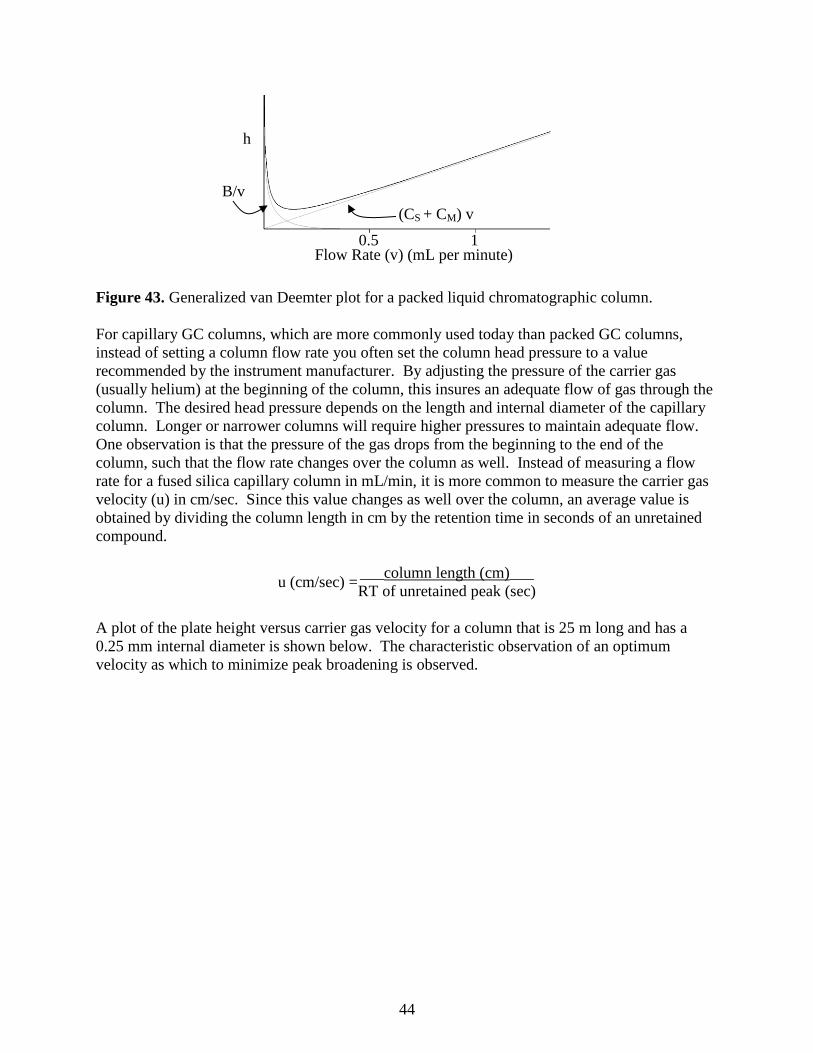
44

Figure 43. Generalized van Deemter plot for a packed liquid chromatographic column.

For capillary GC columns, which are more commonly used today than packed GC columns,

instead of setting a column flow rate you often set the column head pressure to a value

recommended by the instrument manufacturer. By adjusting the pressure of the carrier gas

(usually helium) at the beginning of the column, this insures an adequate flow of gas through the

column. The desired head pressure depends on the length and internal diameter of the capillary

column. Longer or narrower columns will require higher pressures to maintain adequate flow.

One observation is that the pressure of the gas drops from the beginning to the end of the

column, such that the flow rate changes over the column as well. Instead of measuring a flow

rate for a fused silica capillary column in mL/min, it is more common to measure the carrier gas

velocity (u) in cm/sec. Since this value changes as well over the column, an average value is

obtained by dividing the column length in cm by the retention time in seconds of an unretained

compound.

u (cm/sec) = ___column length (cm)___

RT of unretained peak (sec)

A plot of the plate height versus carrier gas velocity for a column that is 25 m long and has a

0.25 mm internal diameter is shown below. The characteristic observation of an optimum

velocity as which to minimize peak broadening is observed.

Flow Rate (v) (mL per minute)

h

B/v

(CS + CM) v

0.5 1

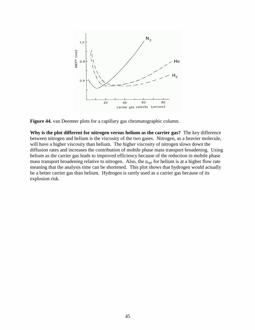
45

Figure 44. van Deemter plots for a capillary gas chromatographic column.

Why is the plot different for nitrogen versus helium as the carrier gas? The key difference

between nitrogen and helium is the viscosity of the two gases. Nitrogen, as a heavier molecule,

will have a higher viscosity than helium. The higher viscosity of nitrogen slows down the

diffusion rates and increases the contribution of mobile phase mass transport broadening. Using

helium as the carrier gas leads to improved efficiency because of the reduction in mobile phase

mass transport broadening relative to nitrogen. Also, the uopt for helium is at a higher flow rate

meaning that the analysis time can be shortened. This plot shows that hydrogen would actually

be a better carrier gas than helium. Hydrogen is rarely used as a carrier gas because of its

explosion risk.

46

FUNDAMENTAL RESOLUTION EQUATION

Another important equation in chromatographic separations is the fundamental resolution

equation. The equation relates the resolution of two compounds (RS) to the number of

theoretical plates (N), retention or capacity factor (k), and selectivity factor (). Appendix I

shows the derivation of the fundamental resolution equation. Since we would usually be

interested in separating two compounds that are close to each other in a chromatogram, and

therefore possibly not resolved, we usually think of applying this equation when we want to

improve the resolution of two adjacent components.

RS = (√N

4) (

α − 1

α) (

k2

1 + k2

)

The interesting part about this equation is that it is possible to examine a chromatogram with

poor resolution, decide which of the three terms is causing the most serious problem, and then

make systematic experimental changes to improve the results. It is worth examining the types of

experimental changes that can be made to influence each of these terms. Notice that in each

case, making the term larger will improve the resolution.

N - Number of theoretical plates

One obvious way to increase the number of plates is to increase the length of the column.

Doubling the length doubles the number of theoretical plates. One cautionary note about this is

to consider the square root dependency on the number of plates in the equation. Doubling the

column length will double the analysis time, but will not double the resolution. We would need

a column four times longer to achieve a doubling of the resolution. Increasing the number of

plates will always give better resolution, but there are diminishing returns when the increased

analysis time is considered.

Another thing to examine is factors that influence the band broadening equation. That equation

related broadening to h, and the smaller the value of h, the more plates in a column. One thing

we could do is optimize the flow rate of the system. We mentioned how it was common to use a

flow rate higher than the optimal one to shorten the analysis time. Slowing down the flow rate

may provide enough gains in efficiency to separate two compounds that are not fully resolved.

Another change to make is to use smaller particles. In gas chromatography, this will lead to a

thinner coating, improving mass transport broadening in the stationary phase. In both gas

chromatography and liquid chromatography, smaller particles will reduce the interstitial volume

and reduce mobile phase mass transport broadening. Smaller particles, provided they are packed

well, also will reduce broadening contributions from eddy diffusion.

47

- Selectivity factor

The first thing to notice about this term is that there are diminishing returns to resolution as it is

made excessively large. Table 1 provides values of and ( – 1)/.

Table 1. Values of and ( – 1)/.

α (α – 1)/α

1 0

2 12⁄

3 23⁄

4 34⁄

5 45⁄

6 56⁄

Notice that the ( – 1)/ term approaches a value of 1 at high values of Optimal -values for

most separations are between 2 and 5.

Remember that the -value refers to the ratio of the two partition coefficients for the two

components. If we wanted to make a substantive change in , we need to change the partition

coefficient of one component but not the other (or we need to change both appreciably but

differently to impact the ratio). There is really only one way to do this and it involves changing

the identity of the stationary phase. This would involve using a different liquid phase in gas

chromatography. As we will see, there are many available liquid phases for use in gas

chromatography, so changing the nature of this phase and hence the -values is a common

procedure.

In liquid chromatography, this would mean switching from a C18 to some other bonded phase.

Since the range of bonded phases is more limited and changes of questionable utility in many

instances, this is not done that frequently. One thing you might wonder about is whether

changing the nature of the mobile phase in liquid chromatography would be viewed as

constituting a change in . This is easily done and is the most common way in liquid

chromatography to improve the resolution of two substances that are not fully resolved. It turns

out that changes to the mobile phase are generally regarded as changes to the retention or

capacity factor. Usually this might involve altering some aspect of the mobile phase so that all

the compounds exhibit a higher capacity, stay on the column longer, and exhibit better

resolution.

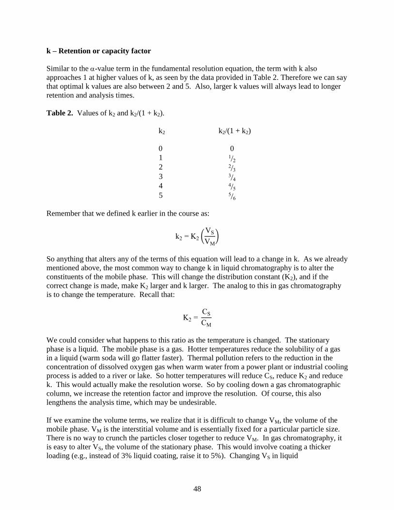
48

k – Retention or capacity factor

Similar to the -value term in the fundamental resolution equation, the term with k also

approaches 1 at higher values of k, as seen by the data provided in Table 2. Therefore we can say

that optimal k values are also between 2 and 5. Also, larger k values will always lead to longer

retention and analysis times.

Table 2. Values of k2 and k2/(1 + k2).

k2 k2/(1 + k2)

0 0

1 12⁄

2 23⁄

3 34⁄

4 45⁄

5 56⁄

Remember that we defined k earlier in the course as:

k2 = K2 (VS

VM

)

So anything that alters any of the terms of this equation will lead to a change in k. As we already

mentioned above, the most common way to change k in liquid chromatography is to alter the

constituents of the mobile phase. This will change the distribution constant (K2), and if the

correct change is made, make K2 larger and k larger. The analog to this in gas chromatography

is to change the temperature. Recall that:

K2 = CS

CM

We could consider what happens to this ratio as the temperature is changed. The stationary

phase is a liquid. The mobile phase is a gas. Hotter temperatures reduce the solubility of a gas

in a liquid (warm soda will go flatter faster). Thermal pollution refers to the reduction in the

concentration of dissolved oxygen gas when warm water from a power plant or industrial cooling

process is added to a river or lake. So hotter temperatures will reduce CS, reduce K2 and reduce

k. This would actually make the resolution worse. So by cooling down a gas chromatographic

column, we increase the retention factor and improve the resolution. Of course, this also

lengthens the analysis time, which may be undesirable.

If we examine the volume terms, we realize that it is difficult to change VM, the volume of the

mobile phase. VM is the interstitial volume and is essentially fixed for a particular particle size.

There is no way to crunch the particles closer together to reduce VM. In gas chromatography, it

is easy to alter VS, the volume of the stationary phase. This would involve coating a thicker

loading (e.g., instead of 3% liquid coating, raise it to 5%). Changing VS in liquid

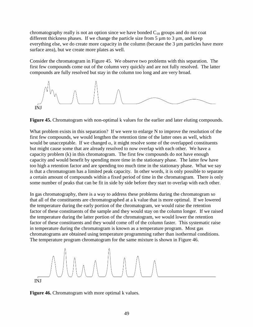
49

chromatography really is not an option since we have bonded C18 groups and do not coat

different thickness phases. If we change the particle size from 5 µm to 3 µm, and keep

everything else, we do create more capacity in the column (because the 3 µm particles have more

surface area), but we create more plates as well.

Consider the chromatogram in Figure 45. We observe two problems with this separation. The

first few compounds come out of the column very quickly and are not fully resolved. The latter

compounds are fully resolved but stay in the column too long and are very broad.

Figure 45. Chromatogram with non-optimal k values for the earlier and later eluting compounds.

What problem exists in this separation? If we were to enlarge N to improve the resolution of the

first few compounds, we would lengthen the retention time of the latter ones as well, which

would be unacceptable. If we changed , it might resolve some of the overlapped constituents

but might cause some that are already resolved to now overlap with each other. We have a

capacity problem (k) in this chromatogram. The first few compounds do not have enough

capacity and would benefit by spending more time in the stationary phase. The latter few have

too high a retention factor and are spending too much time in the stationary phase. What we say

is that a chromatogram has a limited peak capacity. In other words, it is only possible to separate

a certain amount of compounds within a fixed period of time in the chromatogram. There is only

some number of peaks that can be fit in side by side before they start to overlap with each other.

In gas chromatography, there is a way to address these problems during the chromatogram so

that all of the constituents are chromatographed at a k value that is more optimal. If we lowered

the temperature during the early portion of the chromatogram, we would raise the retention

factor of these constituents of the sample and they would stay on the column longer. If we raised

the temperature during the latter portion of the chromatogram, we would lower the retention

factor of these constituents and they would come off of the column faster. This systematic raise

in temperature during the chromatogram is known as a temperature program. Most gas

chromatograms are obtained using temperature programming rather than isothermal conditions.

The temperature program chromatogram for the same mixture is shown in Figure 46.

Figure 46. Chromatogram with more optimal k values.

INJ

INJ

50

There is an analogous procedure in liquid chromatography that is known as gradient elution. In

this technique, you start with a mobile phase that causes the constituents of the sample to have a

high retention factor and then systematically vary the mobile phase during the run to lower the

capacity of the constituents. The exact nature of the changes that might be made to accomplish

this will be discussed later in our unit.

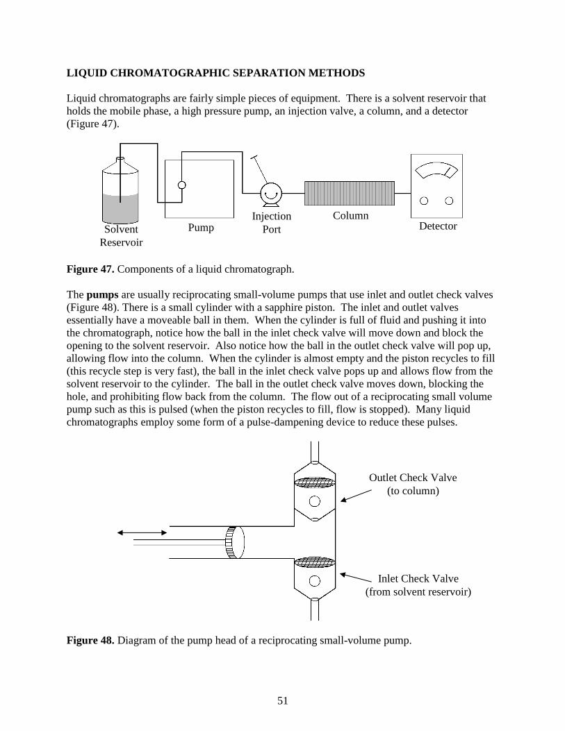
51

LIQUID CHROMATOGRAPHIC SEPARATION METHODS

Liquid chromatographs are fairly simple pieces of equipment. There is a solvent reservoir that

holds the mobile phase, a high pressure pump, an injection valve, a column, and a detector

(Figure 47).

Figure 47. Components of a liquid chromatograph.

The pumps are usually reciprocating small-volume pumps that use inlet and outlet check valves

(Figure 48). There is a small cylinder with a sapphire piston. The inlet and outlet valves

essentially have a moveable ball in them. When the cylinder is full of fluid and pushing it into

the chromatograph, notice how the ball in the inlet check valve will move down and block the

opening to the solvent reservoir. Also notice how the ball in the outlet check valve will pop up,

allowing flow into the column. When the cylinder is almost empty and the piston recycles to fill

(this recycle step is very fast), the ball in the inlet check valve pops up and allows flow from the

solvent reservoir to the cylinder. The ball in the outlet check valve moves down, blocking the

hole, and prohibiting flow back from the column. The flow out of a reciprocating small volume

pump such as this is pulsed (when the piston recycles to fill, flow is stopped). Many liquid

chromatographs employ some form of a pulse-dampening device to reduce these pulses.

Figure 48. Diagram of the pump head of a reciprocating small-volume pump.

Solvent

Reservoir

Injection

Port Pump Column

Detector

Outlet Check Valve

(to column)

Inlet Check Valve

(from solvent reservoir)

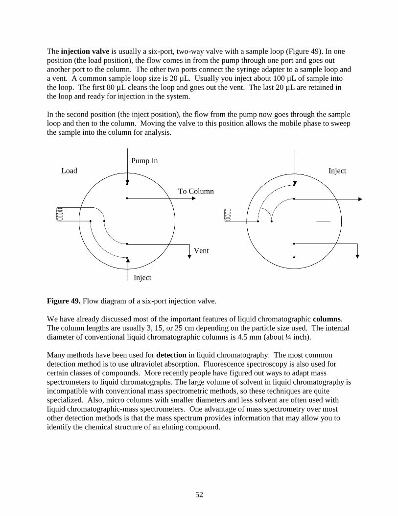
52

The injection valve is usually a six-port, two-way valve with a sample loop (Figure 49). In one

position (the load position), the flow comes in from the pump through one port and goes out

another port to the column. The other two ports connect the syringe adapter to a sample loop and

a vent. A common sample loop size is 20 µL. Usually you inject about 100 µL of sample into

the loop. The first 80 µL cleans the loop and goes out the vent. The last 20 µL are retained in

the loop and ready for injection in the system.

In the second position (the inject position), the flow from the pump now goes through the sample

loop and then to the column. Moving the valve to this position allows the mobile phase to sweep

the sample into the column for analysis.

Figure 49. Flow diagram of a six-port injection valve.

We have already discussed most of the important features of liquid chromatographic columns.

The column lengths are usually 3, 15, or 25 cm depending on the particle size used. The internal

diameter of conventional liquid chromatographic columns is 4.5 mm (about ¼ inch).

Many methods have been used for detection in liquid chromatography. The most common

detection method is to use ultraviolet absorption. Fluorescence spectroscopy is also used for

certain classes of compounds. More recently people have figured out ways to adapt mass

spectrometers to liquid chromatographs. The large volume of solvent in liquid chromatography is

incompatible with conventional mass spectrometric methods, so these techniques are quite

specialized. Also, micro columns with smaller diameters and less solvent are often used with

liquid chromatographic-mass spectrometers. One advantage of mass spectrometry over most

other detection methods is that the mass spectrum provides information that may allow you to

identify the chemical structure of an eluting compound.

Load Inject

Pump In

To Column

Vent

Inject

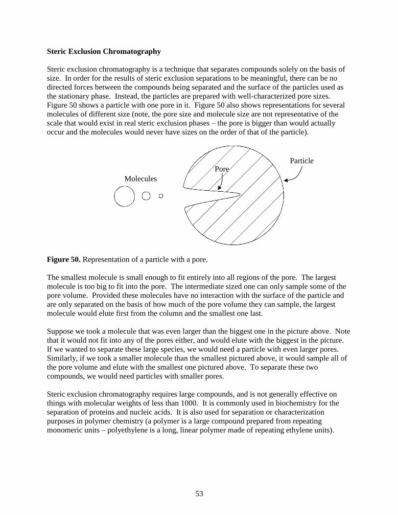
53

Steric Exclusion Chromatography

Steric exclusion chromatography is a technique that separates compounds solely on the basis of

size. In order for the results of steric exclusion separations to be meaningful, there can be no

directed forces between the compounds being separated and the surface of the particles used as

the stationary phase. Instead, the particles are prepared with well-characterized pore sizes.

Figure 50 shows a particle with one pore in it. Figure 50 also shows representations for several

molecules of different size (note, the pore size and molecule size are not representative of the

scale that would exist in real steric exclusion phases – the pore is bigger than would actually

occur and the molecules would never have sizes on the order of that of the particle).

Figure 50. Representation of a particle with a pore.

The smallest molecule is small enough to fit entirely into all regions of the pore. The largest

molecule is too big to fit into the pore. The intermediate sized one can only sample some of the

pore volume. Provided these molecules have no interaction with the surface of the particle and

are only separated on the basis of how much of the pore volume they can sample, the largest

molecule would elute first from the column and the smallest one last.

Suppose we took a molecule that was even larger than the biggest one in the picture above. Note

that it would not fit into any of the pores either, and would elute with the biggest in the picture.

If we wanted to separate these large species, we would need a particle with even larger pores.

Similarly, if we took a smaller molecule than the smallest pictured above, it would sample all of

the pore volume and elute with the smallest one pictured above. To separate these two

compounds, we would need particles with smaller pores.

Steric exclusion chromatography requires large compounds, and is not generally effective on

things with molecular weights of less than 1000. It is commonly used in biochemistry for the

separation of proteins and nucleic acids. It is also used for separation or characterization

purposes in polymer chemistry (a polymer is a large compound prepared from repeating

monomeric units – polyethylene is a long, linear polymer made of repeating ethylene units).

Particle

Molecules

Pore

54

One critical question is how to remove the possibility of an attractive force between the

compounds being separated and the surface of the porous particles. The way this is done is to

use a particle with very different properties than the compound being separated, and to use a

solvent that the solutes are very soluble in. For example, if we want to separate proteins or

nucleic acids, which are polar and very soluble in water, we would need to use porous particles

made from an organic material that had a relatively non-polar surface. If we wanted to separate

polyethylenes of different chain lengths, which are non-polar, we would dissolve the

polyethylene in a non-polar organic solvent and use porous particles made from a material that

had a highly polar surface. This might involve the use of a polydextran (carbohydrate), which

has hydroxyl groups on the surface of the pores.

The classic organic polymer that has been used to prepare porous particles for the steric

exclusion separation of water-soluble polymers is a co-polymer of styrene and divinylbenzene.

Styrene Divinylbenzene

If we just had styrene, and conducted a polymerization, we would get a long, single-bonded

chain of carbon atoms with phenyl rings attached to it. Linear polystyrenes are soluble in certain

non-polar organic solvents. The divinylbenzene acts as a cross-linking agent that bridges

individual styrene chains (Figure 51). A typical ratio of styrene to divinylbenzene is 12:1. The

cross-linking serves to make the polymer into particles rather than linear chains. The cross-

linked polymer is an insoluble material with a very high molecular weight. By controlling the

reaction conditions including the amount of cross-linker and rate of reaction, it is possible to

make polystyrenes with a range of pore sizes.

Figure 51. Cross-linked styrene-divinylbenzene copolymer.

55

If we think about what is inside the column, there are four important volume terms to consider.

One is the total volume of the column (VT). The second is the interstitial volume between the

particles (VI). The third is the volume of all of the pores (VP). The last one is the actual volume

occupied by the mass of the material that makes up the particles.

It turns out that VI is usually about 0.3 of VT for a column. There is simply no way to crunch the

particles closer together to reduce this term appreciably.

VI = 0.3 VT

It turns out that the maximum pore volume that can be achieved is about 0.4 of VT. If you make

this larger, the particles have more pores than structure, become excessively fragile, and get

crushed as you try to push a liquid mobile phase through the column.

VP = 0.4 VT

Totaling this up, we can write that:

VI + VP = 0.7 VT

Since there are no directed forces in a steric exclusion column, this means that all of the

separation must happen in one column volume, or in 0.7 VT. If we then showed a chromatogram

for a series of compounds being separated on a steric exclusion, it might look like that shown in

Figure 52.

Figure 52. Representation of a chromatogram on a steric exclusion column.

The peak labeled 1, which has the shortest retention time (0.3 VT), corresponds to all molecules

in the sample that had a size that was too large to fit into the pores. It cannot be known whether

this is one compound or a mixture of large compounds. The peak labeled 5, which has the

longest retention time (0.7 VT), corresponds to all molecules in the sample that had a size small

enough to sample all of the pore volume. It cannot be known whether it is one compound or a

mixture of two or more small compounds. The peaks labeled 2 through 4 sample some of the

pore volume depending on their size. The peak labeled 6 elutes with a retention volume that is

greater than 0.7 VT. How would we explain the elution volume of this peak? The only way we

1

2

3

4

5

6

0.3 VT 0.7 VT

Elution Volume

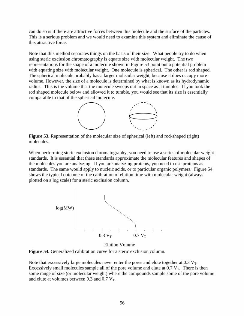
56

can do so is if there are attractive forces between this molecule and the surface of the particles.

This is a serious problem and we would need to examine this system and eliminate the cause of

this attractive force.

Note that this method separates things on the basis of their size. What people try to do when

using steric exclusion chromatography is equate size with molecular weight. The two

representations for the shape of a molecule shown in Figure 53 point out a potential problem

with equating size with molecular weight. One molecule is spherical. The other is rod shaped.

The spherical molecule probably has a larger molecular weight, because it does occupy more

volume. However, the size of a molecule is determined by what is known as its hydrodynamic

radius. This is the volume that the molecule sweeps out in space as it tumbles. If you took the

rod shaped molecule below and allowed it to tumble, you would see that its size is essentially

comparable to that of the spherical molecule.

Figure 53. Representation of the molecular size of spherical (left) and rod-shaped (right)

molecules.

When performing steric exclusion chromatography, you need to use a series of molecular weight

standards. It is essential that these standards approximate the molecular features and shapes of

the molecules you are analyzing. If you are analyzing proteins, you need to use proteins as

standards. The same would apply to nucleic acids, or to particular organic polymers. Figure 54

shows the typical outcome of the calibration of elution time with molecular weight (always

plotted on a log scale) for a steric exclusion column.

Figure 54. Generalized calibration curve for a steric exclusion column.

Note that excessively large molecules never enter the pores and elute together at 0.3 VT.

Excessively small molecules sample all of the pore volume and elute at 0.7 VT. There is then

some range of size (or molecular weight) where the compounds sample some of the pore volume

and elute at volumes between 0.3 and 0.7 VT.

0.7 VT

Elution Volume

log(MW)

0.3 VT

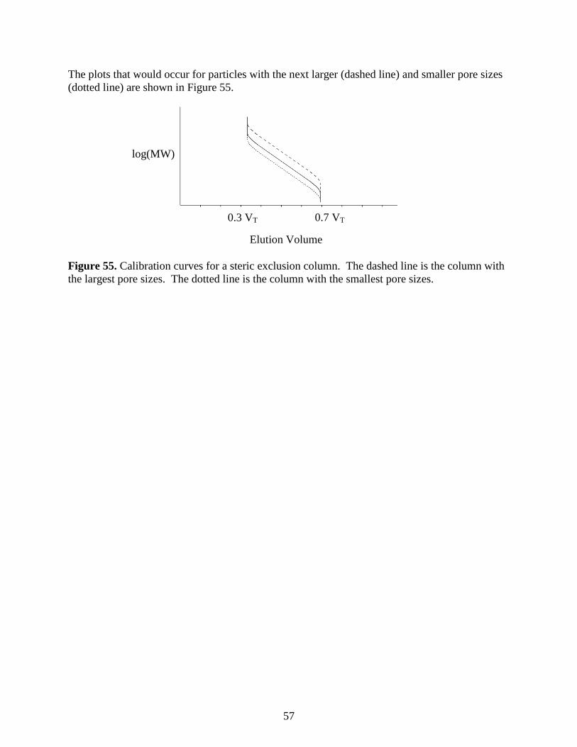
57

The plots that would occur for particles with the next larger (dashed line) and smaller pore sizes

(dotted line) are shown in Figure 55.

Figure 55. Calibration curves for a steric exclusion column. The dashed line is the column with

the largest pore sizes. The dotted line is the column with the smallest pore sizes.

0.7 VT

Elution Volume

log(MW)

0.3 VT

58

Ion-Exchange Chromatography

A second sub-category of liquid chromatography is known as ion-exchange chromatography.

This technique is used to analyze ionic substances. It is often used for inorganic anions (e.g.,

chloride, nitrate, and sulfate) and inorganic cations (e.g., lithium, sodium, and potassium). It can

also be used for organic ions, although this is less common with the advent of reversed phase

liquid chromatographic methods that will be described later. Another significant application of

ion-exchange chromatography is as a step in the purification of proteins. Some of the substituent

groups of amino acids are charged (the total charge for a particular protein is a function of the pH

of the solution), which makes ion exchange a suitable method for protein purification.

The approach is to attach fixed ionic groups to the surface of a solid support. One common

support used in the formation of ion exchange resins is polystyrene-divinylbenzene copolymers.

The fixed ions are attached through a derivatization of the phenyl rings of the polystryene.

Common fixed ions involve either sulfonate groups or quaternary amines as shown in Figure 56.

The aromatic sulfonate groups are strong enough acids that they are deprotonated at all but

highly acidic pH values (pH < 1).

Sulfonate group Quaternary amine

Figure 56. Polystyrene polymer derivatized with fixed ionic groups.

Since we must preserve neutrality in such a system, there must also be an exchangeable

counterion associated with each of these fixed groups. In the case of the sulfonate group, the

counterion is a cation and this is a cation exchange resin. With the quarternary amine phases,

the exchangeable counterion is an anion and this is an anion exchange resin. These counterions

can be exchanged with each other. For example, this would enable you to have a cation

exchange resin in the sodium form or the hydrogen form as seen in Figure 57

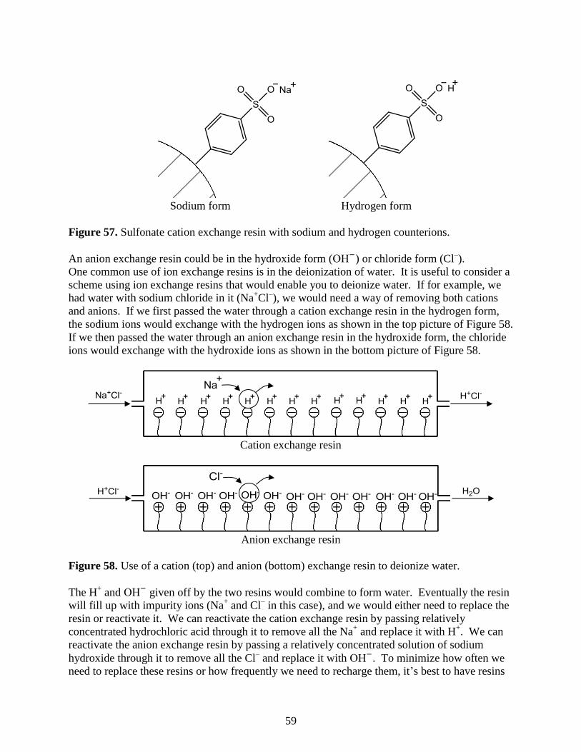
59

Sodium form Hydrogen form

Figure 57. Sulfonate cation exchange resin with sodium and hydrogen counterions.

An anion exchange resin could be in the hydroxide form (OH−

) or chloride form (Cl–).

One common use of ion exchange resins is in the deionization of water. It is useful to consider a

scheme using ion exchange resins that would enable you to deionize water. If for example, we

had water with sodium chloride in it (Na+Cl

–), we would need a way of removing both cations

and anions. If we first passed the water through a cation exchange resin in the hydrogen form,

the sodium ions would exchange with the hydrogen ions as shown in the top picture of Figure 58.

If we then passed the water through an anion exchange resin in the hydroxide form, the chloride

ions would exchange with the hydroxide ions as shown in the bottom picture of Figure 58.

Cation exchange resin

Anion exchange resin

Figure 58. Use of a cation (top) and anion (bottom) exchange resin to deionize water.

The H+ and OH

− given off by the two resins would combine to form water. Eventually the resin

will fill up with impurity ions (Na+ and Cl

– in this case), and we would either need to replace the

resin or reactivate it. We can reactivate the cation exchange resin by passing relatively

concentrated hydrochloric acid through it to remove all the Na+ and replace it with H

+. We can

reactivate the anion exchange resin by passing a relatively concentrated solution of sodium

hydroxide through it to remove all the Cl– and replace it with OH

−. To minimize how often we

need to replace these resins or how frequently we need to recharge them, it’s best to have resins

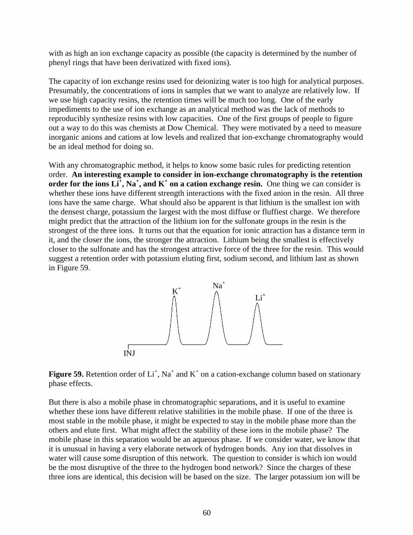
60

with as high an ion exchange capacity as possible (the capacity is determined by the number of

phenyl rings that have been derivatized with fixed ions).

The capacity of ion exchange resins used for deionizing water is too high for analytical purposes.

Presumably, the concentrations of ions in samples that we want to analyze are relatively low. If

we use high capacity resins, the retention times will be much too long. One of the early

impediments to the use of ion exchange as an analytical method was the lack of methods to

reproducibly synthesize resins with low capacities. One of the first groups of people to figure

out a way to do this was chemists at Dow Chemical. They were motivated by a need to measure

inorganic anions and cations at low levels and realized that ion-exchange chromatography would

be an ideal method for doing so.

With any chromatographic method, it helps to know some basic rules for predicting retention

order. An interesting example to consider in ion-exchange chromatography is the retention

order for the ions Li+, Na

+, and K

+ on a cation exchange resin. One thing we can consider is

whether these ions have different strength interactions with the fixed anion in the resin. All three

ions have the same charge. What should also be apparent is that lithium is the smallest ion with

the densest charge, potassium the largest with the most diffuse or fluffiest charge. We therefore

might predict that the attraction of the lithium ion for the sulfonate groups in the resin is the

strongest of the three ions. It turns out that the equation for ionic attraction has a distance term in

it, and the closer the ions, the stronger the attraction. Lithium being the smallest is effectively

closer to the sulfonate and has the strongest attractive force of the three for the resin. This would

suggest a retention order with potassium eluting first, sodium second, and lithium last as shown

in Figure 59.

Figure 59. Retention order of Li+, Na

+ and K

+ on a cation-exchange column based on stationary

phase effects.

But there is also a mobile phase in chromatographic separations, and it is useful to examine

whether these ions have different relative stabilities in the mobile phase. If one of the three is

most stable in the mobile phase, it might be expected to stay in the mobile phase more than the

others and elute first. What might affect the stability of these ions in the mobile phase? The

mobile phase in this separation would be an aqueous phase. If we consider water, we know that

it is unusual in having a very elaborate network of hydrogen bonds. Any ion that dissolves in

water will cause some disruption of this network. The question to consider is which ion would

be the most disruptive of the three to the hydrogen bond network? Since the charges of these

three ions are identical, this decision will be based on the size. The larger potassium ion will be

K+ Na

+

Li+

INJ

61

more disruptive of the hydrogen bonds, and more difficult for water to accommodate. You could

then say that Li+ is more stable in the water, stays in the mobile phase more, and elutes first.

You could phrase this another way by saying that the K+ is least stable in the aqueous mobile

phase, and so is “forced” into the resin by the mobile phase and elutes last. Sometimes the

chromatographic literature refers to this as the solvophobic effect. The K+ fears the solvent and

so spends more time in the resin. The relative retention order based on mobile phase effects

would be lithium first and potassium last, as shown in Figure 60, the exact opposite of what was

predicted above based on stationary phase effects.

Figure 60. Retention order of Li+, Na

+ and K

+ on a cation-exchange column based on mobile

phase effects.

With conflicting predictions, the only way to know which one is more important is to inject the

ions and determine the retention order. In this case, the measurements show that the Li+

elutes first and the K+ elutes last. The mobile phase effects are more significant in determining

the retention order.

Now suppose we had two ions with exactly the same size, but one had a charge of 1+ and the

other a charge of 2+. Examining stationary phase effects, the equation that describes the

attraction between two ions has the charges of both ions in it. The greater the charge of the ions,

the greater the attraction. We would therefore expect the 2+ ion to show greater attraction for the

fixed sulfonate anions and elute later than the 1+ ion as shown in Figure 61.

Figure 61. Retention order on a cation exchange column for ions of the same size but different

charge based on stationary phase effects.

Examining mobile phase effects, both ions would have a similar extent of disruption of the

hydrogen bond network since both have the same size. What we then need to consider is the

strength of the attraction between the positive ion and the sphere of water molecules that

surround it (remember, these cations would be surrounded by the slightly negative oxygen atoms

Li+

K+

Na+

INJ

INJ

+1 +2

62

of water molecules). This represents an electrostatic attraction, and again is dependent on

charge. Therefore the 2+ ion is more stable in the water and ought to elute first as shown in

Figure 62, the exact opposite of what was predicted based on stationary phase effects.

Figure 62. Retention order on a cation exchange column for ions of the same size but different

charge based on mobile phase effects.

Faced with conflicting predictions, it’s necessary to perform the experiment and see which

comes out first. In this case, the measurements show that the 1+ ion elutes first, the 2+ ion

elutes second. The stationary phase effects are more important in this case in determining the

retention order. The likely reason why the stationary phase effects are more significant is that

the 2+ ion can actually bind simultaneously at two adjacent sulfonate sites as shown in Figure

63.

Figure 63. Representation of a +2 ion associating at two anionic sites on the resin.

The likelihood that this occurs can be observed if a lanthanide(III) ion is added to these resins.

In this case, the resin particles actually shrink in size as the lanthanide ion is added. The reason

for the compression is that the binding of three sulfonate groups to the lanthanide causes the

polymer to collapse in a bit to fit these groups around the lanthanide.

The separation of Li+, Na

+, and K

+ described in the prior problem would often be done on a

polystyrene resin using a fairly dilute solution of hydrochloric acid (perhaps 0.1 M) as the mobile

phase. The bound ions would be sulfonate groups and the mobile counter ion would be the H+

ion. An important issue is how to detect these ions. They do not absorb ultraviolet or visible

light in the accessible portion of the spectrum. They do not absorb infrared light. Conductivity

is one possibility for performing the measurement. The conductivity of a solution is a measure

of the extent to which the solution conducts electricity. Dissolved ions are needed for a solution

to conduct electricity, and the higher the concentration of ions, the higher the conductivity. We

can measure the conductivity of a solution quite sensitively. In fact, this is the reading that is

performed on water that has been purified by passage through a MilliQ water purification device

to see just how well the water has been deionized. The only problem with trying to apply a

INJ

+2 +1

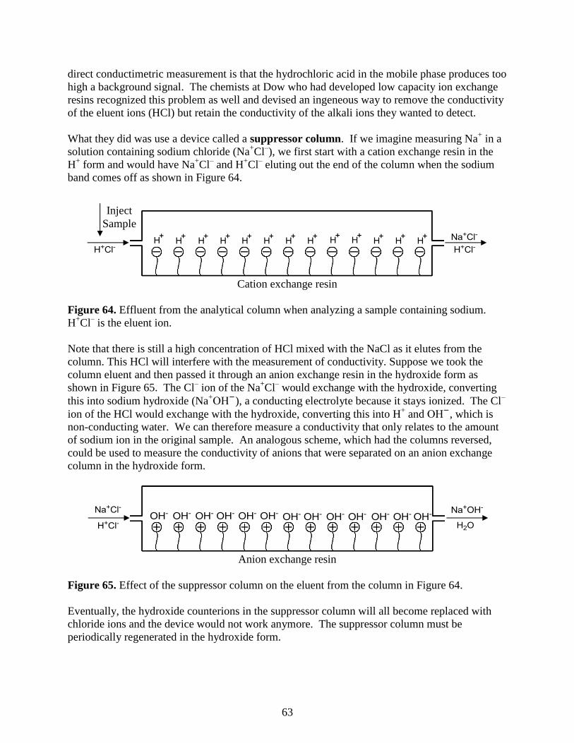
63

direct conductimetric measurement is that the hydrochloric acid in the mobile phase produces too

high a background signal. The chemists at Dow who had developed low capacity ion exchange

resins recognized this problem as well and devised an ingeneous way to remove the conductivity

of the eluent ions (HCl) but retain the conductivity of the alkali ions they wanted to detect.

What they did was use a device called a suppressor column. If we imagine measuring Na+ in a

solution containing sodium chloride (Na+Cl

–), we first start with a cation exchange resin in the

H+ form and would have Na

+Cl

– and H

+Cl

– eluting out the end of the column when the sodium

band comes off as shown in Figure 64.

Cation exchange resin

Figure 64. Effluent from the analytical column when analyzing a sample containing sodium.

H+Cl

– is the eluent ion.

Note that there is still a high concentration of HCl mixed with the NaCl as it elutes from the

column. This HCl will interfere with the measurement of conductivity. Suppose we took the

column eluent and then passed it through an anion exchange resin in the hydroxide form as

shown in Figure 65. The Cl– ion of the Na

+Cl

– would exchange with the hydroxide, converting

this into sodium hydroxide (Na+OH

−), a conducting electrolyte because it stays ionized. The Cl

–

ion of the HCl would exchange with the hydroxide, converting this into H+ and OH

−, which is

non-conducting water. We can therefore measure a conductivity that only relates to the amount

of sodium ion in the original sample. An analogous scheme, which had the columns reversed,

could be used to measure the conductivity of anions that were separated on an anion exchange

column in the hydroxide form.

Anion exchange resin

Figure 65. Effect of the suppressor column on the eluent from the column in Figure 64.

Eventually, the hydroxide counterions in the suppressor column will all become replaced with

chloride ions and the device would not work anymore. The suppressor column must be

periodically regenerated in the hydroxide form.

Inject

Sample

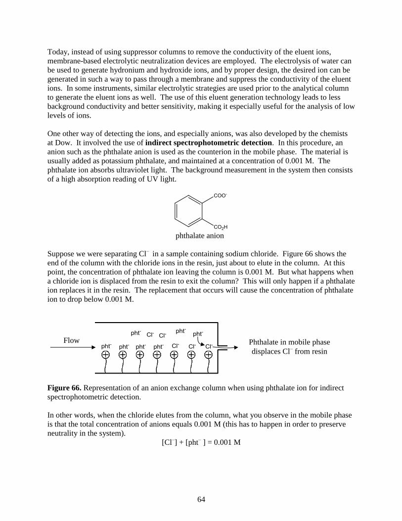
64

Today, instead of using suppressor columns to remove the conductivity of the eluent ions,

membrane-based electrolytic neutralization devices are employed. The electrolysis of water can

be used to generate hydronium and hydroxide ions, and by proper design, the desired ion can be

generated in such a way to pass through a membrane and suppress the conductivity of the eluent

ions. In some instruments, similar electrolytic strategies are used prior to the analytical column

to generate the eluent ions as well. The use of this eluent generation technology leads to less

background conductivity and better sensitivity, making it especially useful for the analysis of low

levels of ions.

One other way of detecting the ions, and especially anions, was also developed by the chemists

at Dow. It involved the use of indirect spectrophotometric detection. In this procedure, an

anion such as the phthalate anion is used as the counterion in the mobile phase. The material is

usually added as potassium phthalate, and maintained at a concentration of 0.001 M. The

phthalate ion absorbs ultraviolet light. The background measurement in the system then consists

of a high absorption reading of UV light.

phthalate anion

Suppose we were separating Cl–

in a sample containing sodium chloride. Figure 66 shows the

end of the column with the chloride ions in the resin, just about to elute in the column. At this

point, the concentration of phthalate ion leaving the column is 0.001 M. But what happens when

a chloride ion is displaced from the resin to exit the column? This will only happen if a phthalate

ion replaces it in the resin. The replacement that occurs will cause the concentration of phthalate

ion to drop below 0.001 M.

Figure 66. Representation of an anion exchange column when using phthalate ion for indirect

spectrophotometric detection.

In other words, when the chloride elutes from the column, what you observe in the mobile phase

is that the total concentration of anions equals 0.001 M (this has to happen in order to preserve

neutrality in the system).

[Cl–] + [pht

– ] = 0.001 M

Flow

Phthalate in mobile phase

displaces Cl– from resin

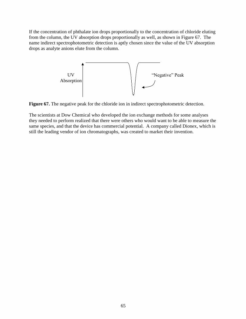
65

If the concentration of phthalate ion drops proportionally to the concentration of chloride eluting

from the column, the UV absorption drops proportionally as well, as shown in Figure 67. The

name indirect spectrophotometric detection is aptly chosen since the value of the UV absorption

drops as analyte anions elute from the column.

Figure 67. The negative peak for the chloride ion in indirect spectrophotometric detection.

The scientists at Dow Chemical who developed the ion exchange methods for some analyses

they needed to perform realized that there were others who would want to be able to measure the

same species, and that the device has commercial potential. A company called Dionex, which is

still the leading vendor of ion chromatographs, was created to market their invention.

UV

Absorption

“Negative” Peak

66

Bonded-phase Liquid Chromatography

In our development of band broadening, we talked extensively about the C18 columns that are the

most common in use today. We already mentioned that less common bonded phases including

those with C8, C1, aminopropyl (C3H6NH2) and cyanopropyl (C3H6CN) groups are also

commercially available. Prior to the introduction of the C18 columns, the normal way to do

liquid chromatography involved the use of a polar stationary phase like silica gel and a non-polar

mobile phase. When the C18 columns were first reported, they constituted a non-polar stationary

phase, and so a polar mobile phase could be employed. Since this configuration of polarities of

the phases was the reverse of what was normally done, the use of C18 columns became known as

reversed-phase liquid chromatography. Even though today almost everyone uses these

reversed-phase methods, the name has stuck.

We have already seen how the deactivation of the surface with the C18 groups has a very positive

effect on the chromatographic efficiency. Another significant advantage of using C18 stationary

phases is that aqueous-based mobile phases are used with them. Water is the ideal mobile phase

for liquid chromatography because so many substances are soluble in water. Water is the solvent

of the environment. Water is the primary solvent of living systems. Many pharmaceutical

agents need to possess water solubility to enter the body. Since many organic compounds are

not that soluble in water, organic pharmaceuticals that are not water-soluble usually have ionic

groups incorporated into them to render them water-soluble.

It’s rare to use only water as the mobile phase with a C18 column. Instead, an organic modifier

(methanol, acetonitrile, and tetrahydrofuran are the three most common) is added in some

amount to the mobile phase. Compared to water, the chemical properties of the organic modifier

are more like that of the C18 phase. The presence of the organic modifier therefore shortens the

retention time compared to a mobile phase that was only water. Raising the concentration of the

organic modifier will further shorten the retention time of almost all compounds. We mentioned

the concept of a gradient elution earlier in the unit when we discussed the problem of having a

limited peak capacity in a chromatogram. Remember the goal was to start with a high retention

factor and systematically change the system so that the retention factor got shorter as the

chromatogram progressed. One possible gradient procedure might be to start with a mobile

phase that is 80:20 water-methanol and gradually change is to 20:80 water-methanol during the

chromatogram. The increased concentration of methanol will reduce the retention factor of the

later eluting components.

Experimentally, it is easy to carry out a gradient. Using two pump heads, one pumps the initial

phase and the other the final phase. A special mixing chamber exists to adequately mix the

output from the two pumps. During the chromatogram, a computer systematically slows down

the pump rate of the initial phase and ramps up the pump rate of the final phase.

Another important variable with an aqueous mobile phase is the pH of the system. C18 silica gel

phases are stable over the range of 2 to 8 (although 3 to 7 really represents a safer window). If

the pH is too acidic, the surface C18 groups will be hydrolyzed off. If the pH is too basic, the

silica gel itself will decompose. This pH range is one that can be used to change the nature of

many acids and bases. For example, carboxylic acids at pH 3 might mostly be in their

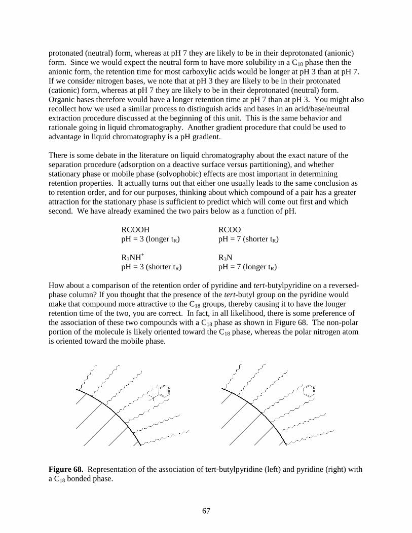
67

protonated (neutral) form, whereas at pH 7 they are likely to be in their deprotonated (anionic)

form. Since we would expect the neutral form to have more solubility in a C18 phase then the

anionic form, the retention time for most carboxylic acids would be longer at pH 3 than at pH 7.

If we consider nitrogen bases, we note that at pH 3 they are likely to be in their protonated

(cationic) form, whereas at pH 7 they are likely to be in their deprotonated (neutral) form.

Organic bases therefore would have a longer retention time at pH 7 than at pH 3. You might also

recollect how we used a similar process to distinguish acids and bases in an acid/base/neutral

extraction procedure discussed at the beginning of this unit. This is the same behavior and

rationale going in liquid chromatography. Another gradient procedure that could be used to

advantage in liquid chromatography is a pH gradient.

There is some debate in the literature on liquid chromatography about the exact nature of the

separation procedure (adsorption on a deactive surface versus partitioning), and whether

stationary phase or mobile phase (solvophobic) effects are most important in determining

retention properties. It actually turns out that either one usually leads to the same conclusion as

to retention order, and for our purposes, thinking about which compound of a pair has a greater

attraction for the stationary phase is sufficient to predict which will come out first and which

second. We have already examined the two pairs below as a function of pH.

RCOOH RCOO–

pH = 3 (longer tR) pH = 7 (shorter tR)

R3NH+ R3N

pH = 3 (shorter tR) pH = 7 (longer tR)

How about a comparison of the retention order of pyridine and tert-butylpyridine on a reversed-

phase column? If you thought that the presence of the tert-butyl group on the pyridine would

make that compound more attractive to the C18 groups, thereby causing it to have the longer

retention time of the two, you are correct. In fact, in all likelihood, there is some preference of

the association of these two compounds with a C18 phase as shown in Figure 68. The non-polar

portion of the molecule is likely oriented toward the C18 phase, whereas the polar nitrogen atom

is oriented toward the mobile phase.

Figure 68. Representation of the association of tert-butylpyridine (left) and pyridine (right) with

a C18 bonded phase.

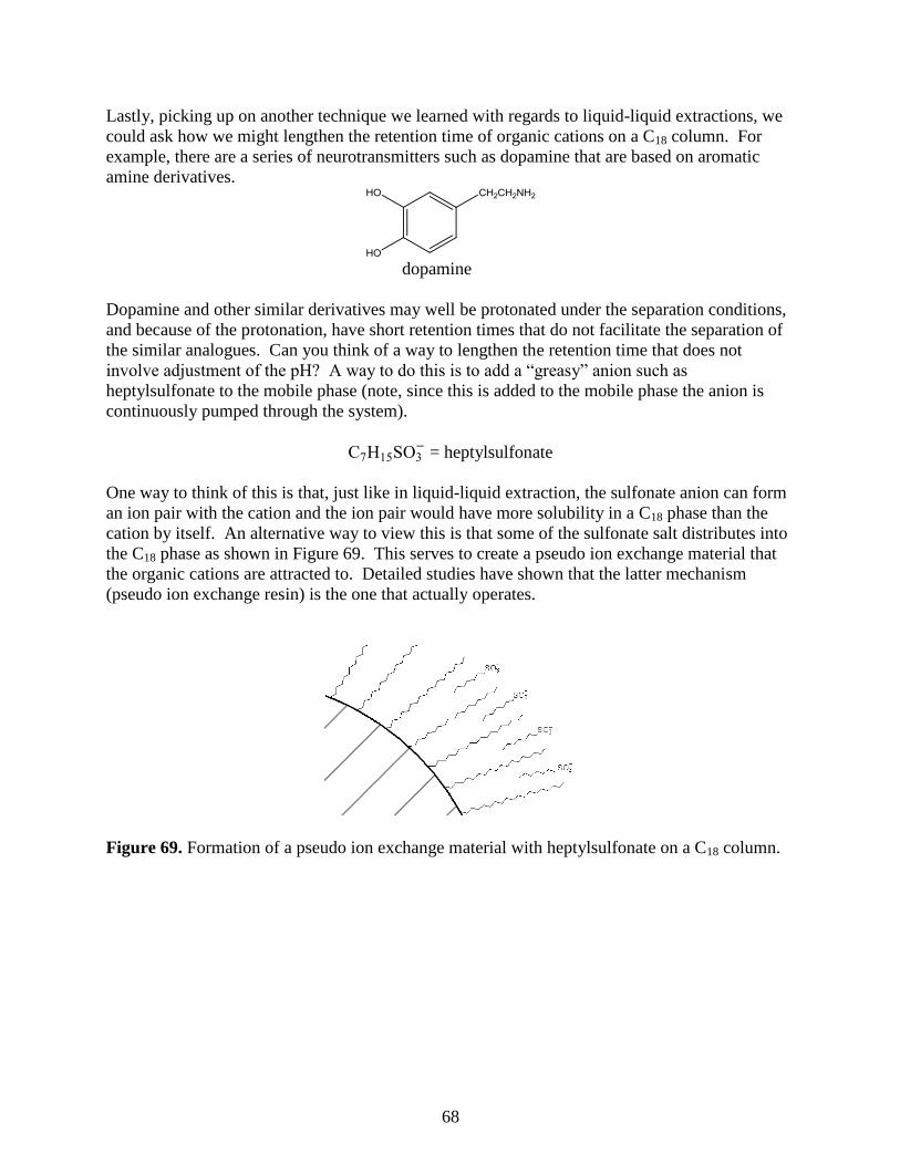
68

Lastly, picking up on another technique we learned with regards to liquid-liquid extractions, we

could ask how we might lengthen the retention time of organic cations on a C18 column. For

example, there are a series of neurotransmitters such as dopamine that are based on aromatic

amine derivatives.

dopamine

Dopamine and other similar derivatives may well be protonated under the separation conditions,

and because of the protonation, have short retention times that do not facilitate the separation of

the similar analogues. Can you think of a way to lengthen the retention time that does not

involve adjustment of the pH? A way to do this is to add a “greasy” anion such as

heptylsulfonate to the mobile phase (note, since this is added to the mobile phase the anion is

continuously pumped through the system).

C7H15SO3−

= heptylsulfonate

One way to think of this is that, just like in liquid-liquid extraction, the sulfonate anion can form

an ion pair with the cation and the ion pair would have more solubility in a C18 phase than the

cation by itself. An alternative way to view this is that some of the sulfonate salt distributes into

the C18 phase as shown in Figure 69. This serves to create a pseudo ion exchange material that

the organic cations are attracted to. Detailed studies have shown that the latter mechanism

(pseudo ion exchange resin) is the one that actually operates.

Figure 69. Formation of a pseudo ion exchange material with heptylsulfonate on a C18 column.

69

One other important category of bonded phases involves the attachment of optically pure groups

to silica gel. The compound dinitrobenzoyl-L-leucine is one example of such a phase. These

types of phases are used for the separation of enantiomers.

The distinction of enantiomers is analogous to the distinction that would occur if you considered

putting your feet into only one of your shoes. If you put your left foot into your left shoe, it feels

fine. If you put your right foot into your left shoe, it does not fit quite as well, and even in the

dark, you would notice that something isn’t right. If we expressed this as a reaction with an

equilibrium constant, we could say that the association of your left foot with your left shoe is

higher than the association of your right foot with your left shoe. If we had bonded the left shoes

to silica gel, your right foot would elute faster from the column, your left foot slower. The

compound pictured above has a number of groups that can form intermolecular interactions with

enantiomeric solutes. The amide functionality is a site with dipoles and the potential for

hydrogen bonding. The electron-deficient dinitrobenzoyl ring can undergo what is known as pi-

stacking with electron-rich aromatic rings. The isobutyl group of the leucine provides steric

hindrance. Other chiral liquid chromatographic phases are designed to have similar groups that

provide sites for intermolecular attraction, -stacking, and steric constraints.

Dinitrobenzoyl-L-leucine

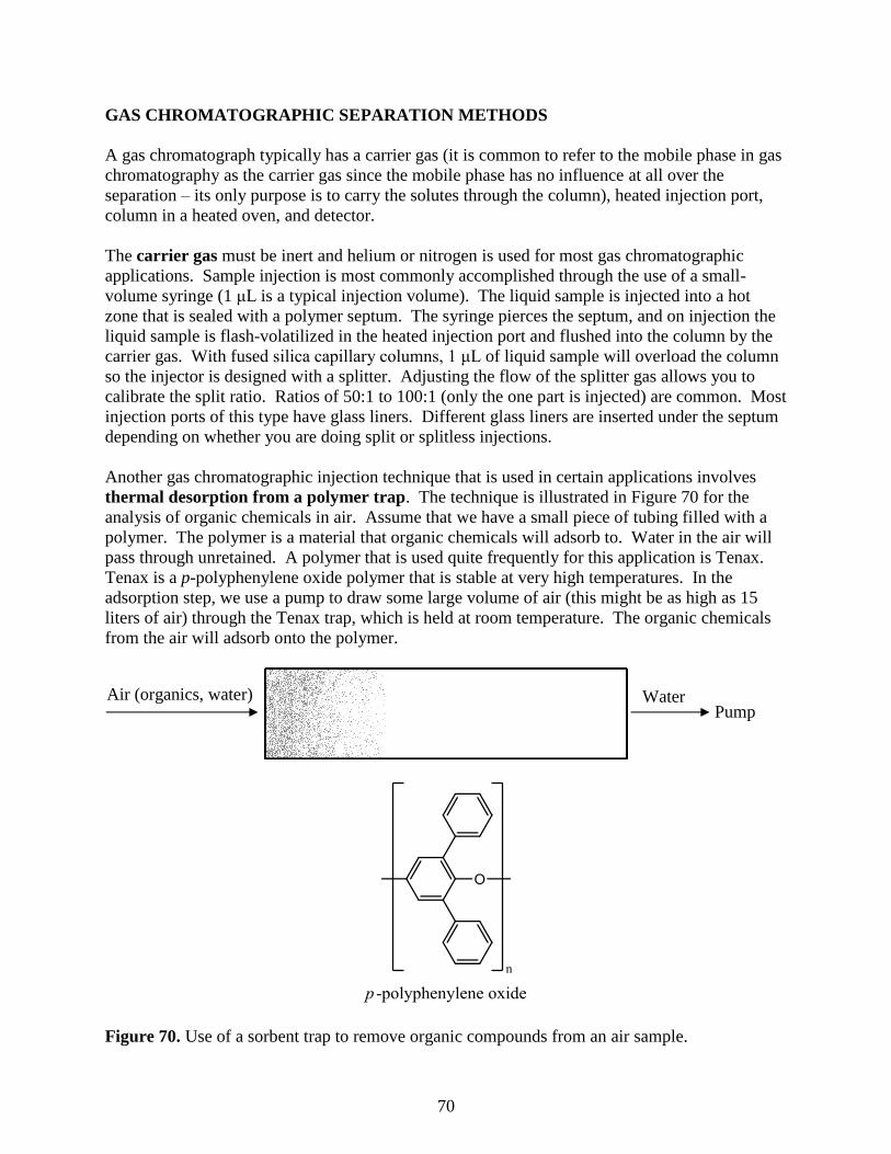
70

GAS CHROMATOGRAPHIC SEPARATION METHODS

A gas chromatograph typically has a carrier gas (it is common to refer to the mobile phase in gas

chromatography as the carrier gas since the mobile phase has no influence at all over the

separation – its only purpose is to carry the solutes through the column), heated injection port,

column in a heated oven, and detector.

The carrier gas must be inert and helium or nitrogen is used for most gas chromatographic

applications. Sample injection is most commonly accomplished through the use of a small-

volume syringe (1 μL is a typical injection volume). The liquid sample is injected into a hot

zone that is sealed with a polymer septum. The syringe pierces the septum, and on injection the

liquid sample is flash-volatilized in the heated injection port and flushed into the column by the

carrier gas. With fused silica capillary columns, 1 μL of liquid sample will overload the column

so the injector is designed with a splitter. Adjusting the flow of the splitter gas allows you to

calibrate the split ratio. Ratios of 50:1 to 100:1 (only the one part is injected) are common. Most

injection ports of this type have glass liners. Different glass liners are inserted under the septum

depending on whether you are doing split or splitless injections.

Another gas chromatographic injection technique that is used in certain applications involves

thermal desorption from a polymer trap. The technique is illustrated in Figure 70 for the

analysis of organic chemicals in air. Assume that we have a small piece of tubing filled with a

polymer. The polymer is a material that organic chemicals will adsorb to. Water in the air will

pass through unretained. A polymer that is used quite frequently for this application is Tenax.

Tenax is a p-polyphenylene oxide polymer that is stable at very high temperatures. In the

adsorption step, we use a pump to draw some large volume of air (this might be as high as 15

liters of air) through the Tenax trap, which is held at room temperature. The organic chemicals

from the air will adsorb onto the polymer.

Figure 70. Use of a sorbent trap to remove organic compounds from an air sample.

Air (organics, water) Water Pump

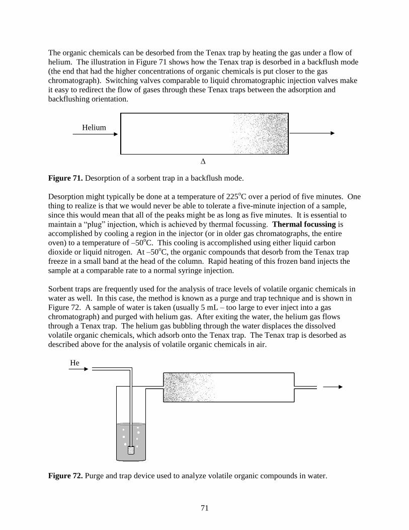
71

The organic chemicals can be desorbed from the Tenax trap by heating the gas under a flow of

helium. The illustration in Figure 71 shows how the Tenax trap is desorbed in a backflush mode

(the end that had the higher concentrations of organic chemicals is put closer to the gas

chromatograph). Switching valves comparable to liquid chromatographic injection valves make

it easy to redirect the flow of gases through these Tenax traps between the adsorption and

backflushing orientation.

Figure 71. Desorption of a sorbent trap in a backflush mode.

Desorption might typically be done at a temperature of 225oC over a period of five minutes. One

thing to realize is that we would never be able to tolerate a five-minute injection of a sample,

since this would mean that all of the peaks might be as long as five minutes. It is essential to

maintain a “plug” injection, which is achieved by thermal focussing. Thermal focussing is

accomplished by cooling a region in the injector (or in older gas chromatographs, the entire

oven) to a temperature of –50oC. This cooling is accomplished using either liquid carbon

dioxide or liquid nitrogen. At –50oC, the organic compounds that desorb from the Tenax trap

freeze in a small band at the head of the column. Rapid heating of this frozen band injects the

sample at a comparable rate to a normal syringe injection.

Sorbent traps are frequently used for the analysis of trace levels of volatile organic chemicals in

water as well. In this case, the method is known as a purge and trap technique and is shown in

Figure 72. A sample of water is taken (usually 5 mL – too large to ever inject into a gas

chromatograph) and purged with helium gas. After exiting the water, the helium gas flows

through a Tenax trap. The helium gas bubbling through the water displaces the dissolved

volatile organic chemicals, which adsorb onto the Tenax trap. The Tenax trap is desorbed as

described above for the analysis of volatile organic chemicals in air.

Figure 72. Purge and trap device used to analyze volatile organic compounds in water.

Helium

Δ

He

72

Another adsorption technique analogous to the sorbent traps discussed above involves the use of

solid phase microextraction (SPME). SPME employs a specially designed syringe in which

the metal barrel that is inserted through the septum of the injection port is wider in diameter than

a usual GC syringe. Inside this wider barrel is a small fiber and a suitable solid adsorbent is

coated onto the fiber. A common SPME procedure would involve the analysis of volatile

organic compounds dissolved in water. A known volume of the water is put into a special vial

that has a cap with a septum. The vial is not filled completely but has a layer of air between the

solution and cap (this is known as the headspace). The syringe needle is inserted through the

septum and a device on the syringe is used to push the fiber out of the syringe barrel. Depending

on the particulars of the analysis, the fiber can be either in the headspace or in the liquid sample.

After a specific adsorption time, the fiber is drawn back into the barrel of the syringe. The

sample is injected into the GC by inserting the syringe through the septum on the injection port

and pushing the fiber out to allow desorption to occur.

Information on a variety of commercially available gas chromatographic stationary phases is

provided in Table 3. The distinction between different stationary phases is based on a

comparison of their polarity. Five different compounds are typically used to represent different

types of functional groups. Individual indices for these five compounds are measured, and a

composite value (P) is determined as well. These polarity indices are referred to as

Rohrschneider constants. The higher the number the more polar the phase. In reality, a

sampling of four or five stationary phases would be good enough to span the range of polarities

that is needed for gas chromatographic separations.

Table 3. Rohrschneider constants for gas chromatographic liquid phases

Liquid phase Max T oC X' Y' Z' U' S' P

Squalane 100 0 0 0 0 0 0

Apiezon L 250 32 22 15 32 42 29

SE-30 300 15 53 44 64 41 43

OV-1, methyl gum 350 16 55 44 65 42 44

OV-3, 10% phenyl 350 44 86 81 124 88 85

OV-7, 20% phenyl 350 69 113 111 171 128 118

Dioctyl sebacate 125 72 168 108 180 123 130

Dilauryl phthalate - 79 158 120 192 158 141

Dinonyl phthalate 150 83 183 147 231 159 161

OV-17, 50% phenyl 375 119 158 162 243 202 177

Versamid 930 150 109 313 144 211 209 197

Trimer acid 150 94 271 163 182 328 218

OV-25, 75% phenyl 350 178 204 208 305 280 235

Polyphenylether 225 182 233 228 313 293 250

Triton X-305 200 262 467 314 488 430 392

Carbowax 20M 225 322 536 368 572 510 462

Carbowax 1540 175 371 639 453 666 641 554

Diglycerol 100 371 826 560 676 854 657

Ethylene glycol phthalate 200 453 697 602 816 872 688

Diethylene glycol succinate 200 496 746 590 837 835 701

Tetrahydroxyethylenediamine 150 463 942 626 - 893 731

Hexakis(2-cyanoethoxycyclohexane) 150 567 825 713 978 901 797

N,N-bis(2-cyanoethyl)formamide 125 690 991 853 1110 1000 929

X' = benzene; Y' = butanol; Z' = 2-pentanone; U' = nitropropane; S' = pyridine, P = (X' + Y' + Z' + U' + S')/5

73

If we consider what governs retention order in gas chromatography, there are two important

parameters. One is the volatility of the compound, with the observation that more volatile

compounds (those with a higher vapor pressure or lower boiling point) elute first. The other is

the attractive forces between the compound and the stationary phase. If we consider the

homologous series of alcohols listed in Table 4, it’s interesting to note that the boiling point goes

up by approximately 20oC for each additional methylene group (CH2) in the chain. The increase

in boiling point with each additional methylene group is a little higher for the series of alkanes.

The alcohols have higher boiling points than the corresponding alkanes because they can

hydrogen bond with each other.

Table 4. Boiling points for homologous series of alkanes and primary alcohols.

Hydrocarbon Boiling Point (oC) Alcohol Boiling Point (

oC)

Pentane 36 1-Pentanol 137

Hexane 69 1-Hexanol 157

Heptane 98 1-Heptanol 176

Octane 126 1-Octanol 196

Nonane 151 1-Nonanol 215

Decane 174 1-Decanol 231

If we consider a homologous series, it turns out that the boiling points are actually determined by

the molar volumes of the molecules. Just as we observed with the size of molecules in steric

exclusion chromatography, the molar volume of a molecule is the volume swept out by the

molecule as it tumbles. Molecules with larger molar volumes have higher boiling points,

provided the molecules being compared have identical intermolecular forces (you cannot

compare hydrocarbons to alcohols). An interesting comparison is observed by looking at the

boiling point of n-octane and iso-octane (2,2,4-trimethylpentane).

n-octane (bp = 126oC) iso-octane (bp = 98

oC)

The branched iso-octane would have a smaller molar volume than the linear n-octane, and this is

clearly reflected in the boiling points of the two compounds.

When predicting retention order in gas chromatography, the overriding factor is a comparison of

the boiling points. The compound with the lowest boiling point elutes first. Only when two

compounds have very close boiling points (within 5oC or less) does it become important to

consider the polarity of the compounds and the polarity of the stationary phase. Remember that

like dissolves like, so a polar stationary phase will show more retention of a polar compound.

The Rohrschneider values are used to determine the polarity of the stationary phase.

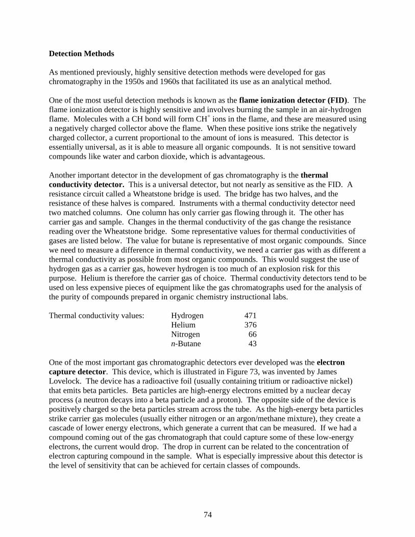
74

Detection Methods

As mentioned previously, highly sensitive detection methods were developed for gas

chromatography in the 1950s and 1960s that facilitated its use as an analytical method.

One of the most useful detection methods is known as the flame ionization detector (FID). The

flame ionization detector is highly sensitive and involves burning the sample in an air-hydrogen

flame. Molecules with a CH bond will form CH+ ions in the flame, and these are measured using

a negatively charged collector above the flame. When these positive ions strike the negatively

charged collector, a current proportional to the amount of ions is measured. This detector is

essentially universal, as it is able to measure all organic compounds. It is not sensitive toward

compounds like water and carbon dioxide, which is advantageous.

Another important detector in the development of gas chromatography is the thermal

conductivity detector. This is a universal detector, but not nearly as sensitive as the FID. A

resistance circuit called a Wheatstone bridge is used. The bridge has two halves, and the

resistance of these halves is compared. Instruments with a thermal conductivity detector need

two matched columns. One column has only carrier gas flowing through it. The other has

carrier gas and sample. Changes in the thermal conductivity of the gas change the resistance

reading over the Wheatstone bridge. Some representative values for thermal conductivities of

gases are listed below. The value for butane is representative of most organic compounds. Since

we need to measure a difference in thermal conductivity, we need a carrier gas with as different a

thermal conductivity as possible from most organic compounds. This would suggest the use of

hydrogen gas as a carrier gas, however hydrogen is too much of an explosion risk for this

purpose. Helium is therefore the carrier gas of choice. Thermal conductivity detectors tend to be

used on less expensive pieces of equipment like the gas chromatographs used for the analysis of

the purity of compounds prepared in organic chemistry instructional labs.

Thermal conductivity values: Hydrogen 471

Helium 376

Nitrogen 66

n-Butane 43

One of the most important gas chromatographic detectors ever developed was the electron

capture detector. This device, which is illustrated in Figure 73, was invented by James

Lovelock. The device has a radioactive foil (usually containing tritium or radioactive nickel)

that emits beta particles. Beta particles are high-energy electrons emitted by a nuclear decay

process (a neutron decays into a beta particle and a proton). The opposite side of the device is

positively charged so the beta particles stream across the tube. As the high-energy beta particles

strike carrier gas molecules (usually either nitrogen or an argon/methane mixture), they create a

cascade of lower energy electrons, which generate a current that can be measured. If we had a

compound coming out of the gas chromatograph that could capture some of these low-energy

electrons, the current would drop. The drop in current can be related to the concentration of

electron capturing compound in the sample. What is especially impressive about this detector is

the level of sensitivity that can be achieved for certain classes of compounds.

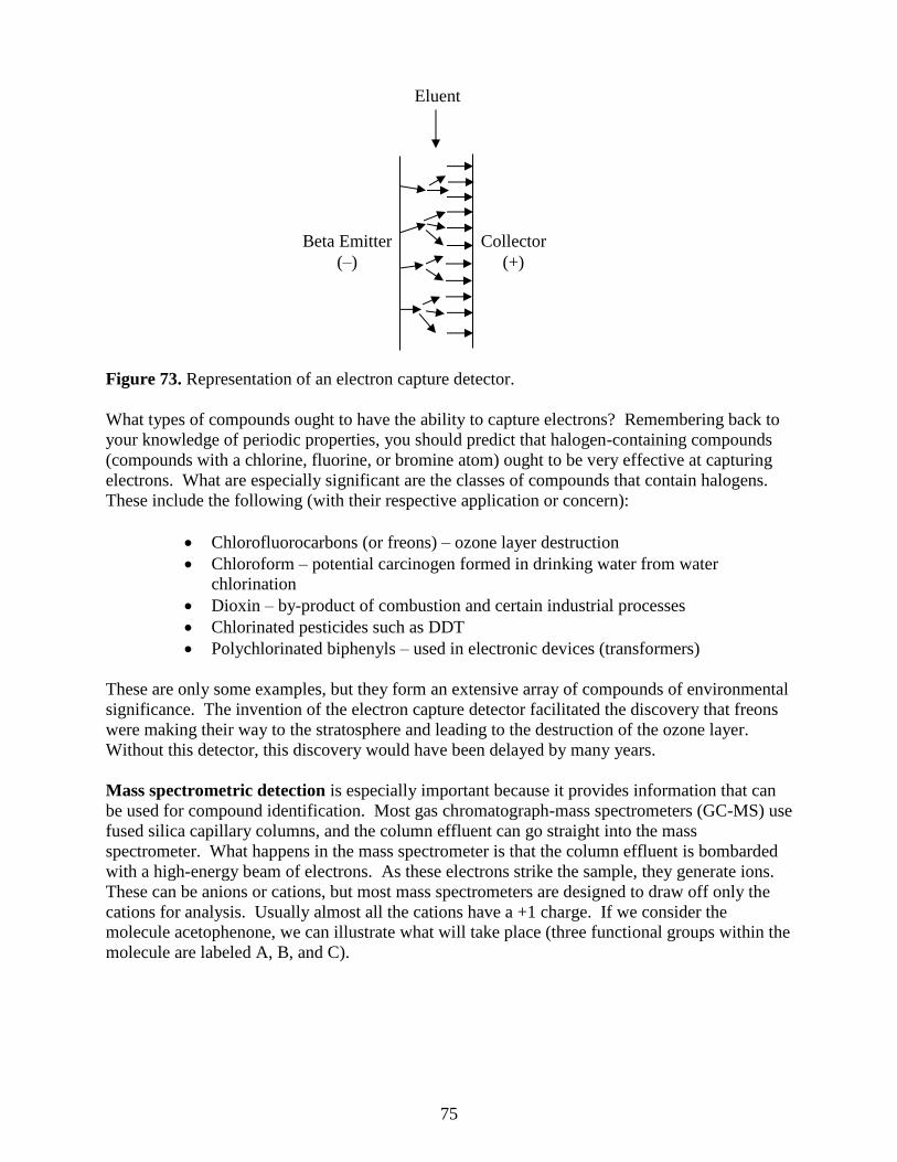
75

Figure 73. Representation of an electron capture detector.

What types of compounds ought to have the ability to capture electrons? Remembering back to

your knowledge of periodic properties, you should predict that halogen-containing compounds

(compounds with a chlorine, fluorine, or bromine atom) ought to be very effective at capturing

electrons. What are especially significant are the classes of compounds that contain halogens.

These include the following (with their respective application or concern):

Chlorofluorocarbons (or freons) – ozone layer destruction

Chloroform – potential carcinogen formed in drinking water from water

chlorination

Dioxin – by-product of combustion and certain industrial processes

Chlorinated pesticides such as DDT

Polychlorinated biphenyls – used in electronic devices (transformers)

These are only some examples, but they form an extensive array of compounds of environmental

significance. The invention of the electron capture detector facilitated the discovery that freons

were making their way to the stratosphere and leading to the destruction of the ozone layer.

Without this detector, this discovery would have been delayed by many years.

Mass spectrometric detection is especially important because it provides information that can

be used for compound identification. Most gas chromatograph-mass spectrometers (GC-MS) use

fused silica capillary columns, and the column effluent can go straight into the mass

spectrometer. What happens in the mass spectrometer is that the column effluent is bombarded

with a high-energy beam of electrons. As these electrons strike the sample, they generate ions.

These can be anions or cations, but most mass spectrometers are designed to draw off only the

cations for analysis. Usually almost all the cations have a +1 charge. If we consider the

molecule acetophenone, we can illustrate what will take place (three functional groups within the

molecule are labeled A, B, and C).

Beta Emitter

(–)

Collector

(+)

Eluent

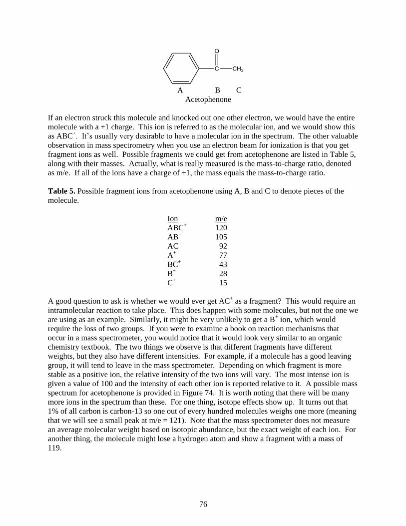
76

A B C

Acetophenone

If an electron struck this molecule and knocked out one other electron, we would have the entire

molecule with a +1 charge. This ion is referred to as the molecular ion, and we would show this

as ABC+. It’s usually very desirable to have a molecular ion in the spectrum. The other valuable

observation in mass spectrometry when you use an electron beam for ionization is that you get

fragment ions as well. Possible fragments we could get from acetophenone are listed in Table 5,

along with their masses. Actually, what is really measured is the mass-to-charge ratio, denoted

as m/e. If all of the ions have a charge of +1, the mass equals the mass-to-charge ratio.

Table 5. Possible fragment ions from acetophenone using A, B and C to denote pieces of the

molecule.

Ion m/e

ABC+

120

AB+

105

AC+

92

A+ 77

BC+ 43

B+

28

C+

15

A good question to ask is whether we would ever get AC+ as a fragment? This would require an

intramolecular reaction to take place. This does happen with some molecules, but not the one we

are using as an example. Similarly, it might be very unlikely to get a B+ ion, which would

require the loss of two groups. If you were to examine a book on reaction mechanisms that

occur in a mass spectrometer, you would notice that it would look very similar to an organic

chemistry textbook. The two things we observe is that different fragments have different

weights, but they also have different intensities. For example, if a molecule has a good leaving

group, it will tend to leave in the mass spectrometer. Depending on which fragment is more

stable as a positive ion, the relative intensity of the two ions will vary. The most intense ion is

given a value of 100 and the intensity of each other ion is reported relative to it. A possible mass

spectrum for acetophenone is provided in Figure 74. It is worth noting that there will be many

more ions in the spectrum than these. For one thing, isotope effects show up. It turns out that

1% of all carbon is carbon-13 so one out of every hundred molecules weighs one more (meaning

that we will see a small peak at m/e = 121). Note that the mass spectrometer does not measure

an average molecular weight based on isotopic abundance, but the exact weight of each ion. For

another thing, the molecule might lose a hydrogen atom and show a fragment with a mass of

119.

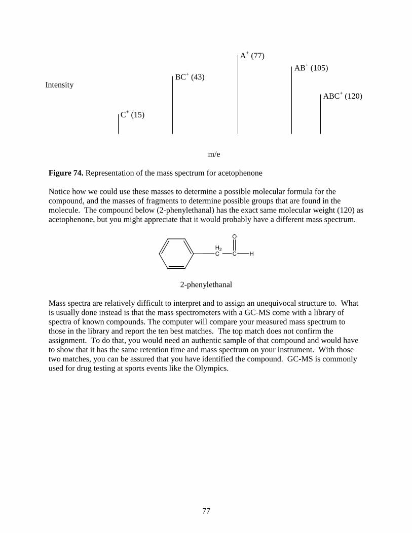
77

Figure 74. Representation of the mass spectrum for acetophenone

Notice how we could use these masses to determine a possible molecular formula for the

compound, and the masses of fragments to determine possible groups that are found in the

molecule. The compound below (2-phenylethanal) has the exact same molecular weight (120) as

acetophenone, but you might appreciate that it would probably have a different mass spectrum.

2-phenylethanal

Mass spectra are relatively difficult to interpret and to assign an unequivocal structure to. What

is usually done instead is that the mass spectrometers with a GC-MS come with a library of

spectra of known compounds. The computer will compare your measured mass spectrum to

those in the library and report the ten best matches. The top match does not confirm the

assignment. To do that, you would need an authentic sample of that compound and would have

to show that it has the same retention time and mass spectrum on your instrument. With those

two matches, you can be assured that you have identified the compound. GC-MS is commonly

used for drug testing at sports events like the Olympics.

C+ (15)

BC+ (43)

A+ (77)

AB+ (105)

ABC+ (120)

Intensity

m/e

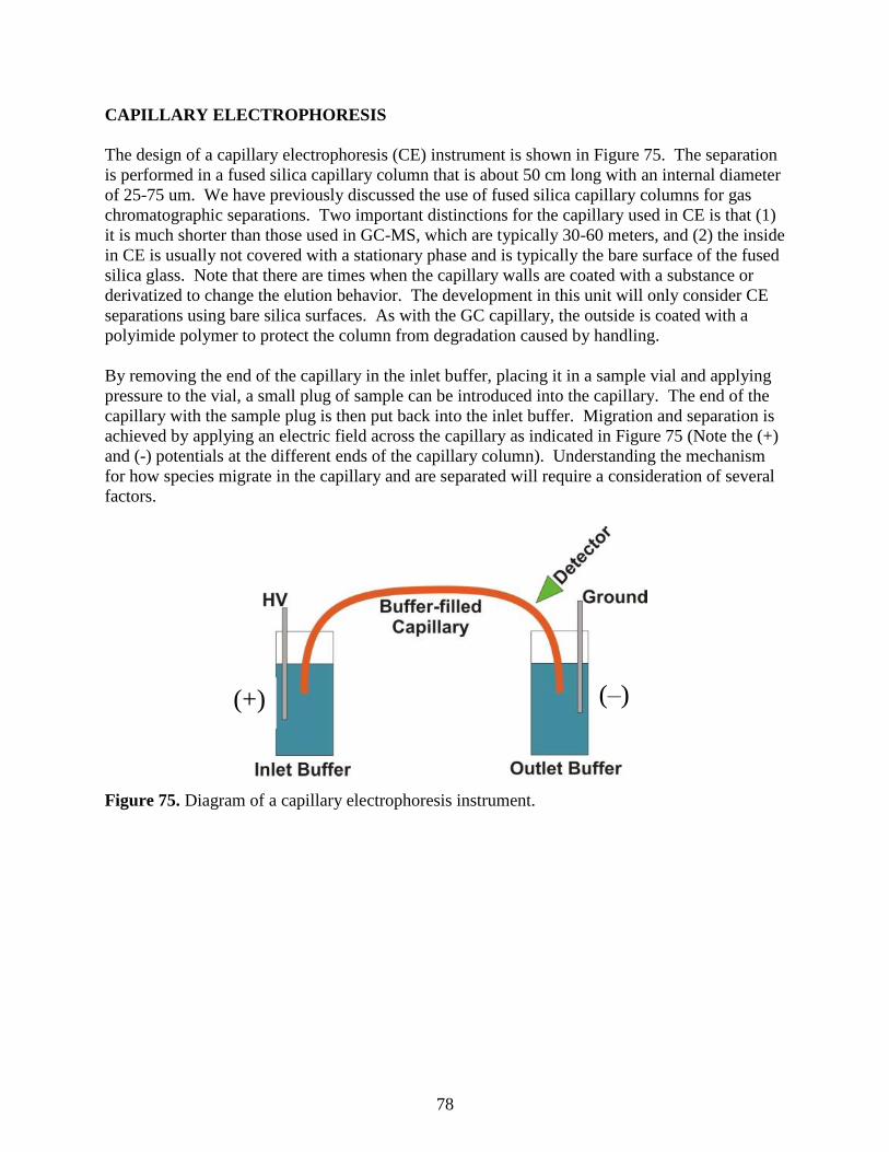
78

CAPILLARY ELECTROPHORESIS

The design of a capillary electrophoresis (CE) instrument is shown in Figure 75. The separation

is performed in a fused silica capillary column that is about 50 cm long with an internal diameter

of 25-75 um. We have previously discussed the use of fused silica capillary columns for gas

chromatographic separations. Two important distinctions for the capillary used in CE is that (1)

it is much shorter than those used in GC-MS, which are typically 30-60 meters, and (2) the inside

in CE is usually not covered with a stationary phase and is typically the bare surface of the fused

silica glass. Note that there are times when the capillary walls are coated with a substance or

derivatized to change the elution behavior. The development in this unit will only consider CE

separations using bare silica surfaces. As with the GC capillary, the outside is coated with a

polyimide polymer to protect the column from degradation caused by handling.

By removing the end of the capillary in the inlet buffer, placing it in a sample vial and applying

pressure to the vial, a small plug of sample can be introduced into the capillary. The end of the

capillary with the sample plug is then put back into the inlet buffer. Migration and separation is

achieved by applying an electric field across the capillary as indicated in Figure 75 (Note the (+)

and (-) potentials at the different ends of the capillary column). Understanding the mechanism

for how species migrate in the capillary and are separated will require a consideration of several

factors.

Figure 75. Diagram of a capillary electrophoresis instrument.

(–) (+)

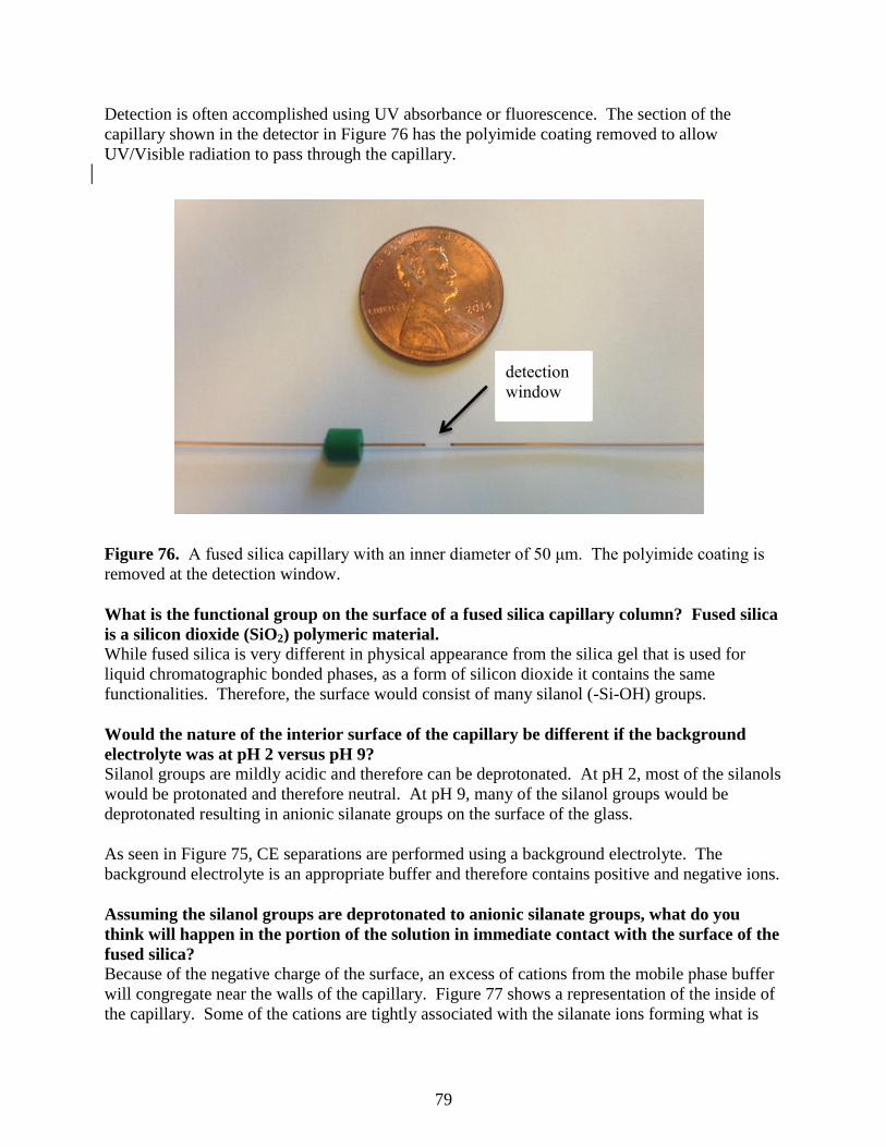
79

Detection is often accomplished using UV absorbance or fluorescence. The section of the

capillary shown in the detector in Figure 76 has the polyimide coating removed to allow

UV/Visible radiation to pass through the capillary.

Figure 76. A fused silica capillary with an inner diameter of 50 μm. The polyimide coating is

removed at the detection window.

What is the functional group on the surface of a fused silica capillary column? Fused silica

is a silicon dioxide (SiO2) polymeric material. While fused silica is very different in physical appearance from the silica gel that is used for

liquid chromatographic bonded phases, as a form of silicon dioxide it contains the same

functionalities. Therefore, the surface would consist of many silanol (-Si-OH) groups.

Would the nature of the interior surface of the capillary be different if the background

electrolyte was at pH 2 versus pH 9?

Silanol groups are mildly acidic and therefore can be deprotonated. At pH 2, most of the silanols

would be protonated and therefore neutral. At pH 9, many of the silanol groups would be

deprotonated resulting in anionic silanate groups on the surface of the glass.

As seen in Figure 75, CE separations are performed using a background electrolyte. The

background electrolyte is an appropriate buffer and therefore contains positive and negative ions.

Assuming the silanol groups are deprotonated to anionic silanate groups, what do you

think will happen in the portion of the solution in immediate contact with the surface of the

fused silica?

Because of the negative charge of the surface, an excess of cations from the mobile phase buffer

will congregate near the walls of the capillary. Figure 77 shows a representation of the inside of

the capillary. Some of the cations are tightly associated with the silanate ions forming what is

detection

window

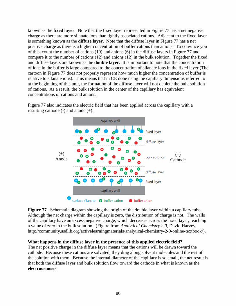
80

known as the fixed layer. Note that the fixed layer represented in Figure 77 has a net negative

charge as there are more silanate ions than tightly associated cations. Adjacent to the fixed layer

is something known as the diffuse layer. Note that the diffuse layer in Figure 77 has a net

positive charge as there is a higher concentration of buffer cations than anions. To convince you

of this, count the number of cations (10) and anions (6) in the diffuse layers in Figure 77 and

compare it to the number of cations (12) and anions (12) in the bulk solution. Together the fixed

and diffuse layers are known as the double layer. It is important to note that the concentration

of ions in the buffer is large compared to the concentration of silanate ions in the fixed layer (The

cartoon in Figure 77 does not properly represent how much higher the concentration of buffer is

relative to silanate ions). This means that in CE done using the capillary dimensions referred to

at the beginning of this unit, the formation of the diffuse layer will not deplete the bulk solution

of cations. As a result, the bulk solution in the center of the capillary has equivalent

concentrations of cations and anions.

Figure 77 also indicates the electric field that has been applied across the capillary with a

resulting cathode (-) and anode (+).

Figure 77. Schematic diagram showing the origin of the double layer within a capillary tube.

Although the net charge within the capillary is zero, the distribution of charge is not. The walls

of the capillary have an excess negative charge, which decreases across the fixed layer, reaching

a value of zero in the bulk solution. (Figure from Analytical Chemistry 2.0, David Harvey,

http://community.asdlib.org/activelearningmaterials/analytical-chemistry-2-0-online-textbook/).

What happens in the diffuse layer in the presence of this applied electric field?

The net positive charge in the diffuse layer means that the cations will be drawn toward the

cathode. Because these cations are solvated, they drag along solvent molecules and the rest of

the solution with them. Because the internal diameter of the capillary is so small, the net result is

that both the diffuse layer and bulk solution flow toward the cathode in what is known as the

electroosmosis.

(–)

Cathode

(+)

Anode

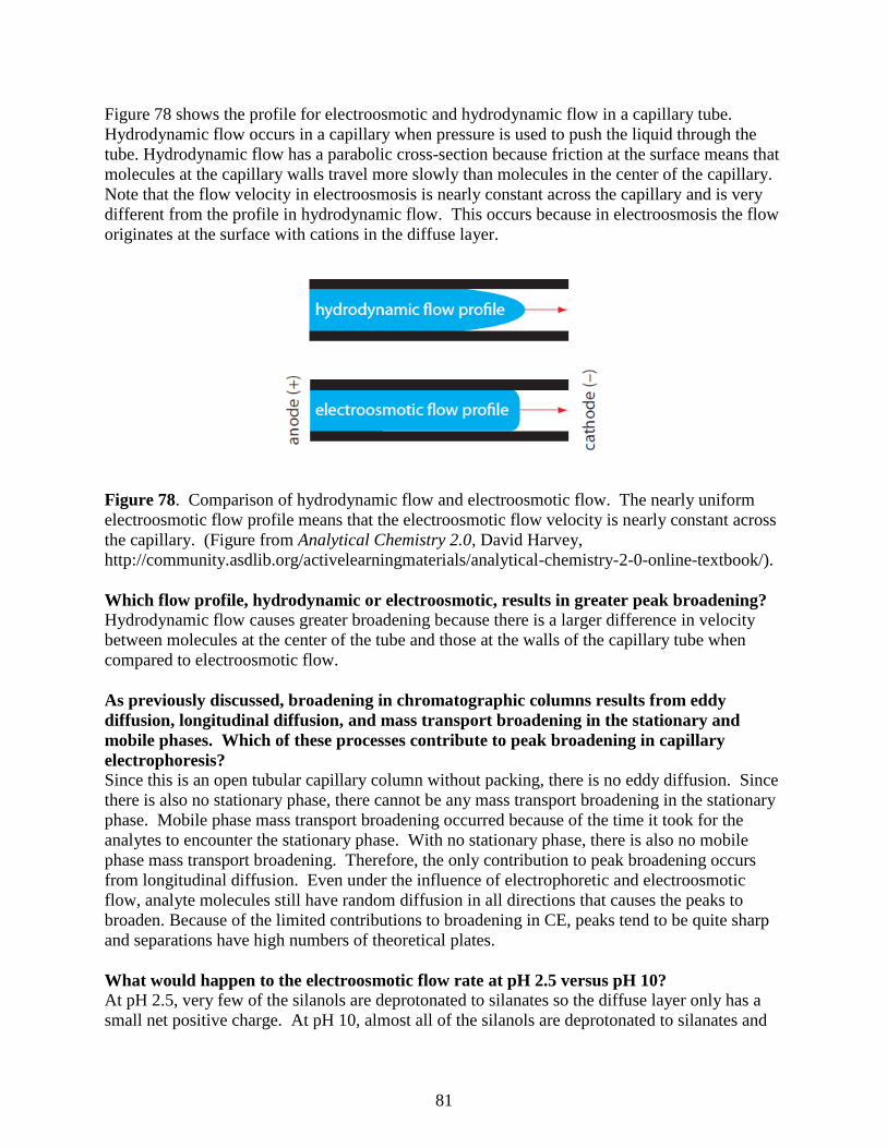
81

Figure 78 shows the profile for electroosmotic and hydrodynamic flow in a capillary tube.

Hydrodynamic flow occurs in a capillary when pressure is used to push the liquid through the

tube. Hydrodynamic flow has a parabolic cross-section because friction at the surface means that

molecules at the capillary walls travel more slowly than molecules in the center of the capillary.

Note that the flow velocity in electroosmosis is nearly constant across the capillary and is very

different from the profile in hydrodynamic flow. This occurs because in electroosmosis the flow

originates at the surface with cations in the diffuse layer.

Figure 78. Comparison of hydrodynamic flow and electroosmotic flow. The nearly uniform

electroosmotic flow profile means that the electroosmotic flow velocity is nearly constant across

the capillary. (Figure from Analytical Chemistry 2.0, David Harvey,

http://community.asdlib.org/activelearningmaterials/analytical-chemistry-2-0-online-textbook/).

Which flow profile, hydrodynamic or electroosmotic, results in greater peak broadening?

Hydrodynamic flow causes greater broadening because there is a larger difference in velocity

between molecules at the center of the tube and those at the walls of the capillary tube when

compared to electroosmotic flow.

As previously discussed, broadening in chromatographic columns results from eddy

diffusion, longitudinal diffusion, and mass transport broadening in the stationary and

mobile phases. Which of these processes contribute to peak broadening in capillary

electrophoresis?

Since this is an open tubular capillary column without packing, there is no eddy diffusion. Since

there is also no stationary phase, there cannot be any mass transport broadening in the stationary

phase. Mobile phase mass transport broadening occurred because of the time it took for the

analytes to encounter the stationary phase. With no stationary phase, there is also no mobile

phase mass transport broadening. Therefore, the only contribution to peak broadening occurs

from longitudinal diffusion. Even under the influence of electrophoretic and electroosmotic

flow, analyte molecules still have random diffusion in all directions that causes the peaks to

broaden. Because of the limited contributions to broadening in CE, peaks tend to be quite sharp

and separations have high numbers of theoretical plates.

What would happen to the electroosmotic flow rate at pH 2.5 versus pH 10?

At pH 2.5, very few of the silanols are deprotonated to silanates so the diffuse layer only has a

small net positive charge. At pH 10, almost all of the silanols are deprotonated to silanates and

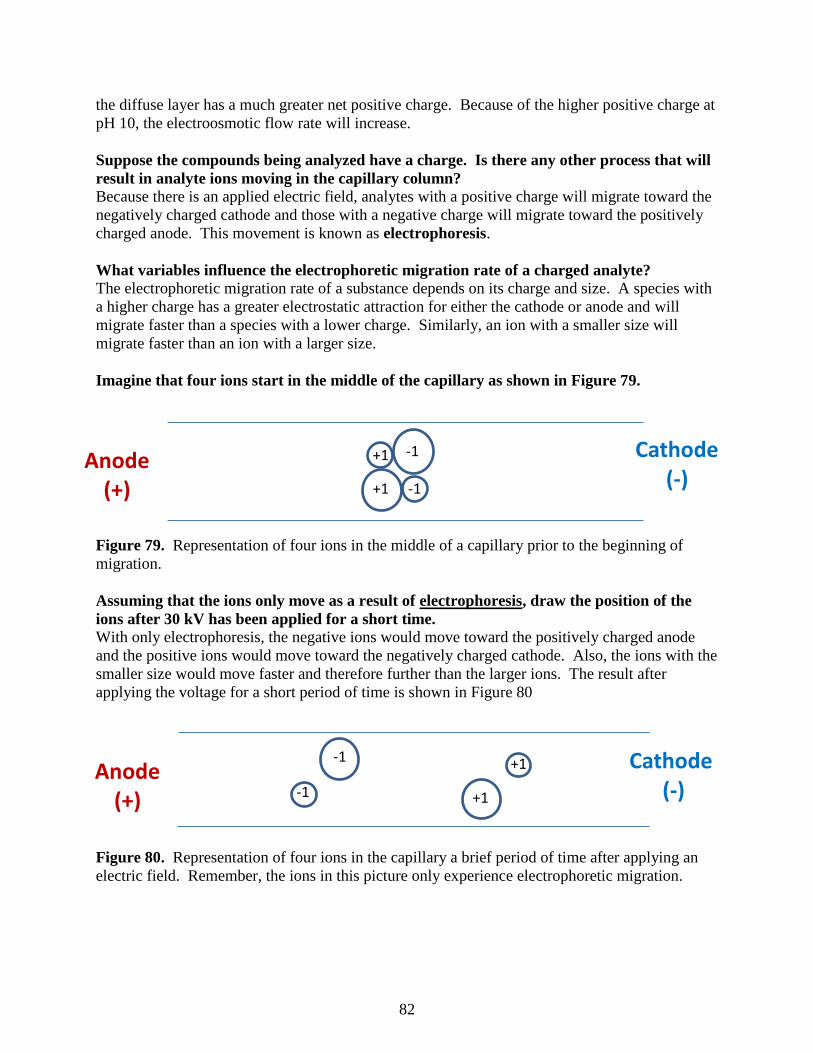
82

the diffuse layer has a much greater net positive charge. Because of the higher positive charge at

pH 10, the electroosmotic flow rate will increase.

Suppose the compounds being analyzed have a charge. Is there any other process that will

result in analyte ions moving in the capillary column?

Because there is an applied electric field, analytes with a positive charge will migrate toward the

negatively charged cathode and those with a negative charge will migrate toward the positively

charged anode. This movement is known as electrophoresis.

What variables influence the electrophoretic migration rate of a charged analyte?

The electrophoretic migration rate of a substance depends on its charge and size. A species with

a higher charge has a greater electrostatic attraction for either the cathode or anode and will

migrate faster than a species with a lower charge. Similarly, an ion with a smaller size will

migrate faster than an ion with a larger size.

Imagine that four ions start in the middle of the capillary as shown in Figure 79.

Figure 79. Representation of four ions in the middle of a capillary prior to the beginning of

migration.

Assuming that the ions only move as a result of electrophoresis, draw the position of the

ions after 30 kV has been applied for a short time.

With only electrophoresis, the negative ions would move toward the positively charged anode

and the positive ions would move toward the negatively charged cathode. Also, the ions with the

smaller size would move faster and therefore further than the larger ions. The result after

applying the voltage for a short period of time is shown in Figure 80

Figure 80. Representation of four ions in the capillary a brief period of time after applying an

electric field. Remember, the ions in this picture only experience electrophoretic migration.

Cathode (-)

Anode (+)

+1

+1

-1

-1

Cathode (-)

Anode (+)

+1

+1

-1

-1

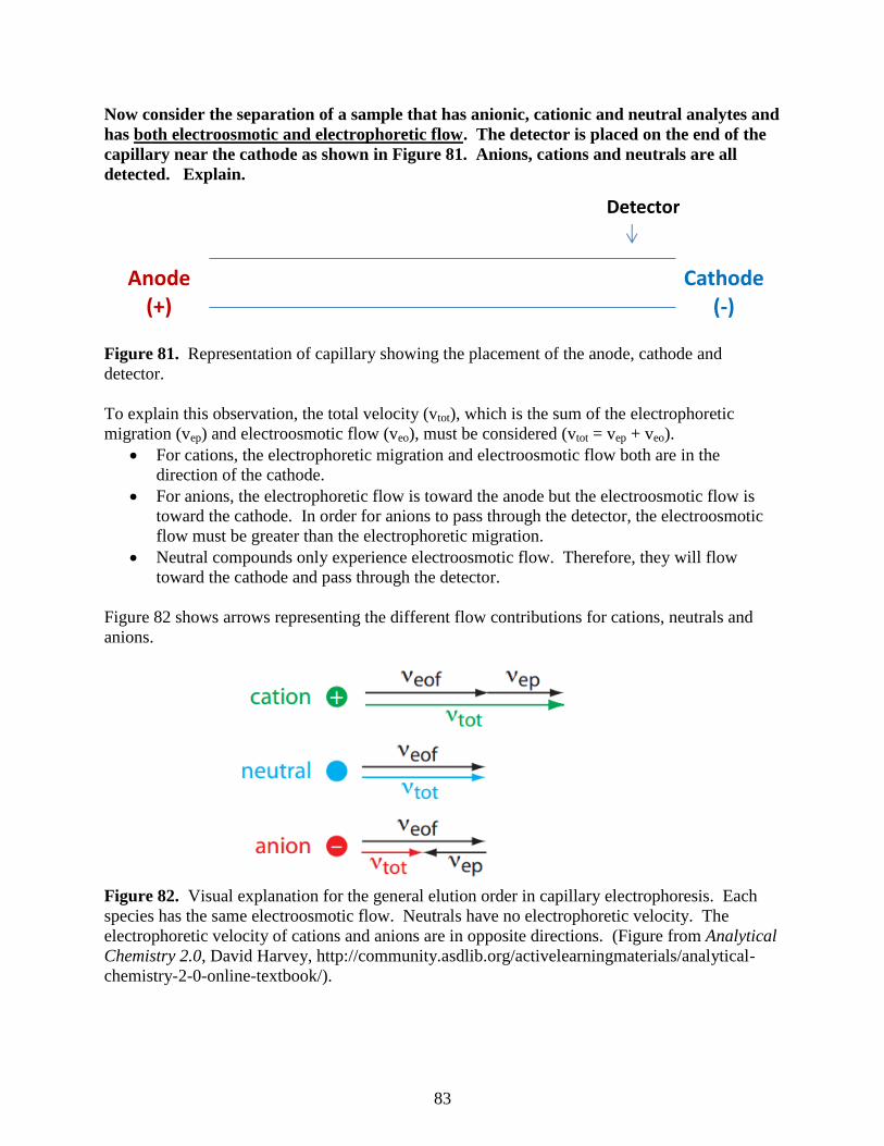
83

Now consider the separation of a sample that has anionic, cationic and neutral analytes and

has both electroosmotic and electrophoretic flow. The detector is placed on the end of the

capillary near the cathode as shown in Figure 81. Anions, cations and neutrals are all

detected. Explain.

Figure 81. Representation of capillary showing the placement of the anode, cathode and

detector.

To explain this observation, the total velocity (vtot), which is the sum of the electrophoretic

migration (vep) and electroosmotic flow (veo), must be considered (vtot = vep + veo).

For cations, the electrophoretic migration and electroosmotic flow both are in the

direction of the cathode.

For anions, the electrophoretic flow is toward the anode but the electroosmotic flow is

toward the cathode. In order for anions to pass through the detector, the electroosmotic

flow must be greater than the electrophoretic migration.

Neutral compounds only experience electroosmotic flow. Therefore, they will flow

toward the cathode and pass through the detector.

Figure 82 shows arrows representing the different flow contributions for cations, neutrals and

anions.

Figure 82. Visual explanation for the general elution order in capillary electrophoresis. Each

species has the same electroosmotic flow. Neutrals have no electrophoretic velocity. The

electrophoretic velocity of cations and anions are in opposite directions. (Figure from Analytical

Chemistry 2.0, David Harvey, http://community.asdlib.org/activelearningmaterials/analytical-

chemistry-2-0-online-textbook/).

Cathode (-)

Anode (+)

Detector

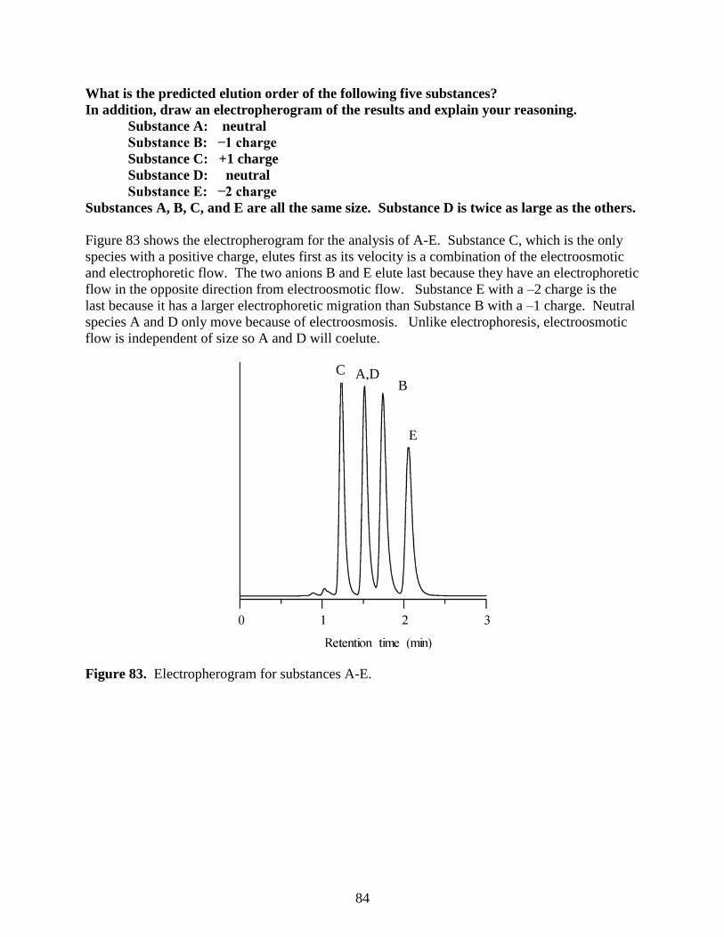
84

What is the predicted elution order of the following five substances?

In addition, draw an electropherogram of the results and explain your reasoning.

Substance A: neutral

Substance B: ̶ 1 charge

Substance C: +1 charge

Substance D: neutral

Substance E: ̶ 2 charge

Substances A, B, C, and E are all the same size. Substance D is twice as large as the others.

Figure 83 shows the electropherogram for the analysis of A-E. Substance C, which is the only

species with a positive charge, elutes first as its velocity is a combination of the electroosmotic

and electrophoretic flow. The two anions B and E elute last because they have an electrophoretic

flow in the opposite direction from electroosmotic flow. Substance E with a –2 charge is the

last because it has a larger electrophoretic migration than Substance B with a –1 charge. Neutral

species A and D only move because of electroosmosis. Unlike electrophoresis, electroosmotic

flow is independent of size so A and D will coelute.

Figure 83. Electropherogram for substances A-E.

C

E

A,D B

85

The structural formulas and relevant pKa values for the four components of an Exedrin

tablet are shown in Figure 84. (The protonated form of the boxed group is shown.) Predict

the elution order in CE with a 20 mM borate buffer at pH = 9.3.

Figure 83. Structures and pKa values of the four primary constituents of Excedrin

The important thing to consider is whether the acidic or basic functional groups are protonated or

deprotonated at pH 9.3 to determine the overall charge of the species.

For aspirin, the carboxylic acid group with a pKa of 3.5 will be “fully deprotonated” so

will have a –l charge. The words “fully deprotonated” are put in quotes because a very

small amount must be protonated to satisfy the Ka expression, but it is so small that it can

be ignored.

For caffeine, the nitrogen atom with a pKa of 10.6 will be “fully protonated” so will have

a charge of +1.

For acetaminophen, the hydroxyl (phenol) group with a pKa of 9.9 is only 0.6 units from

the pH of the buffer. In this case, only a portion of the acetaminophen will be

deprotonated at any given moment and there will be a rapid exchange between protonated

(neutral) and deprotonated (anionic) forms. Therefore, it will have a charge that can be

considered as between 0 and –1.

For salicylic acid, the carboxylic acid group with a pKa of 3.5 will be “fully

deprotonated” whereas the hydroxyl group with a pKa of 13.4 will be “fully protonated”.

The overall charge will be –1.

86

To summarize, at pH 9.3, the species would have the following charges:

Aspirin: –1 charge

Caffeine: +1 charge

Acetaminophen: Average charge between 0 to –1

Salicylic acid: –1 charge

The system is set up such that cations elute first, followed by neutrals and finally followed by

anions. Therefore, caffeine elutes first. Acetaminophen elutes second because it has the smallest

negative charge of the three anionic species. Aspirin and salicylic acid have identical charges

but differ slightly in size with aspirin being slightly larger than salicylic acid. Because aspirin is

larger its electrophoretic migration is less than that of salicylic acid and since the electrophoresis

of anions is opposite of the direction of electroosmotic flow needed for elution, aspirin elutes

before salicylic acid.

What could you do experimentally to confirm your predicted elution order?

You would need to make up solutions with one each of the four compounds and carry out the

analysis to determine their retention time.

An actual electropherogram of this sample at pH 9.3 is shown in Figure 85.

Figure 85. Electropherogram of the four constituents of Excedrin at pH 9.3: caffeine (1.567

min), acetaminophen (1.805 min), aspirin (2.801 min) and salicylic acid (3.308 min).

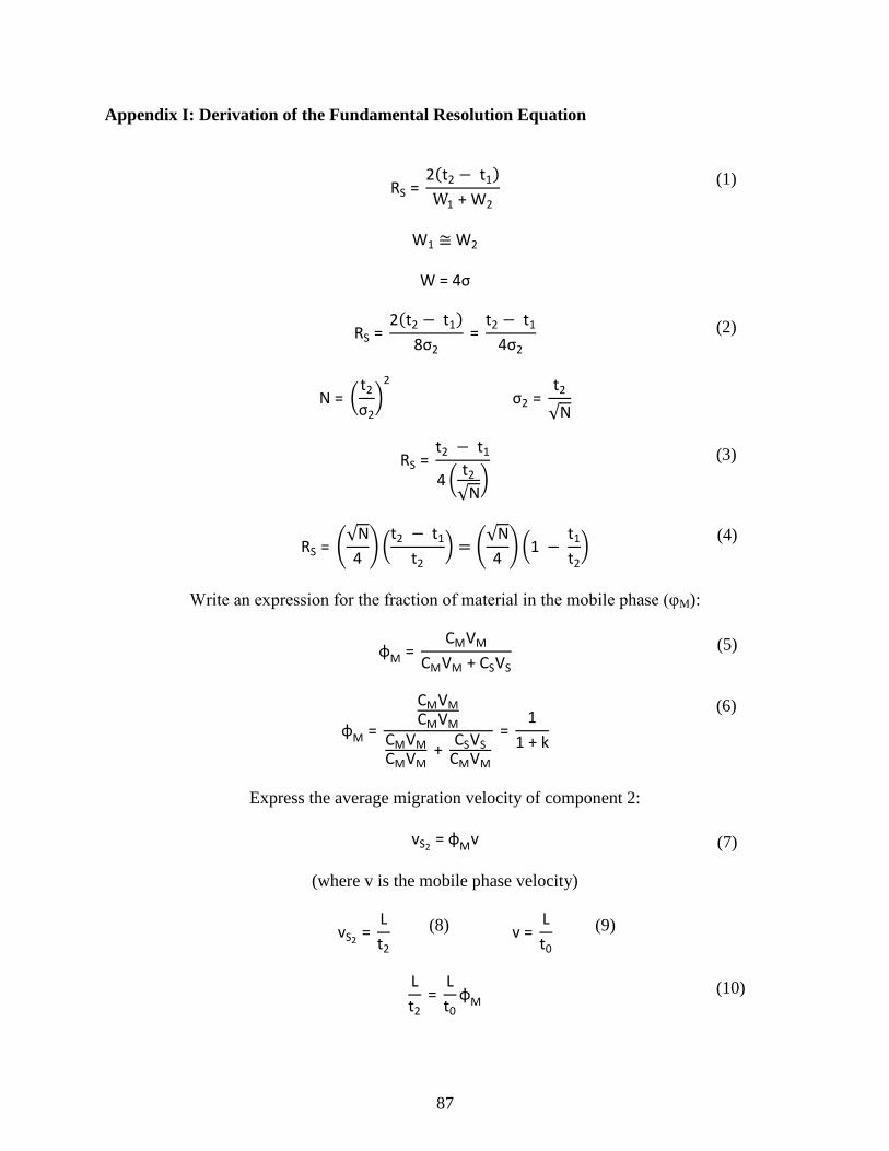
87

Appendix I: Derivation of the Fundamental Resolution Equation

RS = 2(t2 − t1)

W1 + W2

W1 ≅ W2

W = 4σ

RS = 2(t2 − t1)

8σ2 =

t2 − t1

4σ2

N = (t2

σ2)

2

σ2 = t2

√N

RS = t2 − t1

4 (t2

√N)

RS = (√N

4) (

t2 − t1

t2) = (

√N

4) (1 −

t1

t2)

Write an expression for the fraction of material in the mobile phase (φM):

φM = CMVM

CMVM + CSVS

φM =

CMVM

CMVM

CMVM

CMVM +

CSVS

CMVM

= 1

1 + k

Express the average migration velocity of component 2:

vS2 = φMv

(where v is the mobile phase velocity)

vS2 =

L

t2 v =

L

t0

L

t2 =

L

t0φM

(1)

(2)

(6)

(3)

(4)

(5)

(7)

(8) (9)

(10)

88

t2 = t0

φM2

t1 = t0

φM1

t2 = t0

(1

1 + k2)

t1 = t0

(1

1 + k1)

t2 = t0(1 + k2) t1 = t0(1 + k1)

t1

t2 =

t0(1 + k1)

t0(1 + k2) =

1 + k1

1 + k2

Substitute (14) into (4):

RS = (√N

4) (1 −

1 + k1

1 + k2)

Consider the (1 − 1 + k1

1 + k2) term:

(1 −1 + k1

1 + k2) = (

1 + k2

1 + k2 −

1 + k1

1 + k2)

= k2 – k1

1 + k2

= k1 (

k2

k1 − 1)

1 + k2

= (

k2

k1) k1 (

k2

k1 − 1)

( k2

k1) (1 + k2)

= k2 (

k2

k1 − 1)

( k2

k1) (1 + k2)

= (k2

1+ k2) (

k2

k1 − 1

k2

k1

)

α = k2

k1

= (k2

1+ k2) (

α − 1

α)

(11)

(12)

(13)

(14)

(15)

(15a)

(15b)

(15c)

(15d)

(15e)

(15f)

89

Substitute (15f) into (15):

RS = (√N

4) (

α − 1

α) (

k2

1 + k2)

Relationship to retention time:

vS2=

L

t2 t2 =

L

vS2

vS2= φMv = (

1

1 + k2) v

H = L

N L = HN

t2 = HN(1 + k2)

v

Rearrange the fundamental resolution equation to solve for N:

N = 16RS2 (

α

α − 1)

2

(1 + k2

k2)

2

t2 = (16RS

2H

v) (

α

α − 1)

2

((1 + k2)3

(k2)2)

(16)

(17)

(18)