Sensors 2014, 14, 23137-23158; doi:10.3390/s141223137OPEN ACCESS

sensorsISSN 1424-8220

www.mdpi.com/journal/sensors

Article

Correlated Spatio-Temporal Data Collection in Wireless SensorNetworks Based on Low Rank Matrix Approximation andOptimized Node SamplingXinglin Piao 1, Yongli Hu 1, Yanfeng Sun 1,*, Baocai Yin 1 and Junbin Gao 2

1 Beijing Key Laboratory of Multimedia and Intelligent Software Technology, College of MetropolitanTransportation, Beijing University of Technology, Pingleyuan 100, Chaoyang District, Beijing100124, China; E-Mails: piaoxinglin1987@gmail.com (X.P.); huyongli@bjut.edu.cn (Y.H.);ybc@bjut.edu.cn (B.Y.)

2 School of Computing and Mathematics, Charles Sturt University, Bathurst, NSW 2795, Australia;E-Mail: jbgao@csu.edu.au

* Author to whom correspondence should be addressed; E-Mail: yfsun@bjut.edu.cn;Tel.: +86-10-6739-6568 (ext. 2108); Fax: +86-10-6739-6568 (ext. 2115).

External Editor: Leonhard M. Reindl

Received: 16 September 2014; in revised form: 21 November 2014 / Accepted: 26 November 2014 /Published: 5 December 2014

Abstract: The emerging low rank matrix approximation (LRMA) method provides anenergy efficient scheme for data collection in wireless sensor networks (WSNs) by randomlysampling a subset of sensor nodes for data sensing. However, the existing LRMA basedmethods generally underutilize the spatial or temporal correlation of the sensing data,resulting in uneven energy consumption and thus shortening the network lifetime. In thispaper, we propose a correlated spatio-temporal data collection method for WSNs based onLRMA. In the proposed method, both the temporal consistence and the spatial correlationof the sensing data are simultaneously integrated under a new LRMA model. Moreover, thenetwork energy consumption issue is considered in the node sampling procedure. We useGini index to measure both the spatial distribution of the selected nodes and the evennessof the network energy status, then formulate and resolve an optimization problem to achieveoptimized node sampling. The proposed method is evaluated on both the simulated and realwireless networks and compared with state-of-the-art methods. The experimental resultsshow the proposed method efficiently reduces the energy consumption of network andprolongs the network lifetime with high data recovery accuracy and good stability.

Sensors 2014, 14 23138

Keywords: wireless sensor networks; data collection; low rank matrix approximation.

1. Introduction

Data collection is a fundamental application of wireless sensor networks (WSNs). For example, inthe environmental monitoring scenario, the physical quantities, such as temperature, humidity and lightillumination, etc. are usually sensed and transmitted from sensor nodes to sink nodes through multi-hoprouting [1]. Since the sensor nodes usually have limited computing ability and power supply, a primarygoal of data collection is to obtain the sensing data at required accuracy with least energy consumptionand thus to prolong the network lifetime.

Since the physical quantities describing natural phenomena are generally locally consistent and WSNsnodes are often deployed redundantly to get complete environmental monitoring data, the sensing dataoften have high spatial or temporal correlation [2]. Thus many researchers utilize the spatial andtemporal correlation to reduce the network energy consumption by delivering part of sensing data ortheir aggregation, such as distributed source coding techniques [3–5], in-network collaborative wavelettransform methods [6,7] and clustered data aggregation methods [8–11]. Although these methodscan save certain data communication cost, they would bring extra computational overheads for sensornodes and so demand considerable sensing cost. Recently the low rank matrix approximation (LRMA)method [12,13] provides a new scheme for data collection in WSNs [14–16]. The main idea of theLRMA based method is that the sensing data of WSNs are regarded as a low rank matrix and recoveredfrom a subset sensing data. As demonstrated in Figure 1, the data collection consists of two stages: thedata sensing stage and the data recovering stage. At the data sensing stage, instead of using all sensornodes, a subset of sensor nodes which are the shaded ones in the second subfigure is randomly selectedto sense physical quantity and deliver the sensing data to the sink node at each data collection round. Atthe data recovering stage, the sink node receives these incomplete sensing data over some data collectionrounds shown in the third subfigure in which the shaded entries represent the valid sensing data andthe white entries are unknown. And then we could use them to recover the complete data by LRMAmethod. As the LRMA based data collection methods reduce either the data communication cost or thedata sensing cost, high energy efficiency can be achieved even with an increased computation cost at thesink node.

Figure 1. The correlated spatio-temporal data collection method based on LRMA andoptimized node sampling.

WSNs nodesNodes selected for data

sensing at one time slot

Time Slot

NodeIndex

Time Slot

NodeIndex

The incomplete sensing

data matrix

Data recovery based on low

rank matrix approximation

at the sink node

Sensors 2014, 14 23139

However, the current LRMA based data collection methods [14–16] also suffer from certaininefficiency both at the data sensing stage and the data recovering stage. At the data sensing stage, arandom sampling scheme for the selection of sensing nodes is adopted in the current methods [14–16].According to the LRMA theory [13], the uniformly random sampling method is an optimized samplingway to get good matrix complement result. However, the ideal random sampling method will result inuneven energy distribution of the network as the many-to-one data collection pattern, and thus shortenthe network lifetime. At the data recovering stage, most of the current methods do not explore and utilizethe spatial or temporal correlation of the sensing data. This could be the contributing factor to the certainsetback of these methods, such as low data recovery accuracy, and lacking robustness to noises andoutliers. Therefore, to improve the efficiency of the current LRMA based data collection methods, wealways face two challenges. On the one hand, we should find out a proper way to formulate the relationbetween two important components in the data sensing procedure, the node sampling scheme and thescheme of estimating energy status of the network. Generally, the former has direct effect on the datarecovery accuracy, and the later can determine the lifetime of the network. On the other hand, the mainobstacle is how to represent the spatial and temporal relations of the incomplete node sensing data andfurther integrate these constraints to the current LRMA data recovery model. In this paper, we presenta new data collection method based on LRMA, which improves the performance of the current methodboth at the data sensing and data recovering stages. At the data sensing stage, we propose to use Giniindex to measure the spatial distributions of the selected sensing nodes and the evenness of energy statusof the network. Under this measurement, the selection of sensing nodes is formulated as an optimizationproblem with the constraint of the network energy status. At the recovering stage, observing that thesensing data from a sensor generally has temporal consistency and the sensing data from different nodeshas spatial correlation excepting for some noise and outliers. We give the representations of the spatialand temporal relationship of the node sensing data and add these constraints into the basic LRMA modeland construct a correlated spatio-temporal constrained LRMA model (ST-LRMA). Then the ST-LRMAmodel is solved by an iteration method.

The proposed ST-LRMA based data collection method is tested on both simulated and real wirelessnetworks compared with other relevant methods. The experimental results demonstrate the proposedmethod achieves better data recovery accuracy and improves energy efficiency to prolong networklifetime. Additionally, it is robust to noise and outliers.

The main contributions of this paper are:

(1) We propose a correlated spatio-temporal constrained low rank matrix approximation model, anovel data collection scheme in WSNs;

(2) We propose an optimized node sampling model for reducing energy consumption of WSNs, inwhich Gini Index is adopt and used as a tool to improve the current uniformly random samplingmethod.

The rest of the paper is organized as follows. In Section 2, we summarize the related work.Section 3 introduces the basic LRMA model based on random sampling. Section 4 presents the proposedST-LRMA model. Section 5 elaborates the new optimized node sampling method. We will show theexperimental results of our proposed methods compared with state-of-the-art methods, such as basic

Sensors 2014, 14 23140

LRMA model [14], T-LRMA model [15,16] and S-LRMA model in Section 6. Section 7 concludes thepaper with a discussion on future research.

2. Related Works

In many data collection scenarios in WSNs, such as environmental monitoring [17], to fully sensephysical quantities efficiently, it is necessary to transmit all sensing data to the sink node correctly andaccurately. Doing so would consume too much energy in the networks. However, it is unnecessary toget the entire sensing data, given that there exists high correlation in the sensing data. Hence, the beststrategy is to explore energy efficient data collection methods which approximately get the sensing datawith a given accuracy.

The conventional approximate data collection methods include data aggregation techniques,distributed source coding and collaborative in-network compression methods. Data aggregationtechniques [8–11] formulate the network sensor nodes into a hierarchical structure like trees or clusters.Generally the sensing nodes send the sensing data to the middle aggregator nodes. These aggregatorscollect data from multiple sensor nodes and aggregate the sensing data by aggregation functions, andthen send the aggregated results to upper aggregators or sink nodes. Only a subset of nodes is involvedin the communication with an aggregator and thus the overall energy consumption of the network duringdata collection is reduced. Distributed source coding schemes are based on the Slepian-Wolf codingtheory [3–5]. In these methods, the sensor nodes are modeled as correlated sources of information andthe dependency between the measured data are exploited to obtain data compression. Collaborativein-network compression methods can be viewed as an extension of traditional transforms in signalprocessing to sensor networks with irregular topology. Nodes can communicate with their neighbors andspatial correlation is exploited by collaborative transforms such as the distributed wavelet transform [6]and the graph wavelet transform [7].

Although the above mentioned conventional data collection methods are considered to be energyefficient and widely used in WSNs applications, they have their respective advantages in different aspectsand the energy efficiency of these methods is relative to specific application scenarios. For example, theaggregation methods generally depend on a particular routing protocol, and the source coding methodstypically require exact knowledge of the correlation between the measurements of different sensor nodes.It is highly desired to investigate the generic data collection method with high energy efficiency. Thetypical representatives are the recently proposed compressive sensing (CS) based methods [18–22] andthe LRMA based methods [14–16].

The CS based methods provide two features of universal sampling and decentralized encoding, whichmake it a new paradigm for data collection in WSNs. In a single-hop network, a universal compressivewireless sensing method is proposed to deliver the sensing data by synchronized amplitude-modulatedanalog transmissions to the fusion center [23]. The sparsity of the sensing data and the CS decodingalgorithms are discussed for data collection application in [24]. The first complete scheme to applycompressive sensing theory to data collection in large scale sensor networks is presented in [18]. Thenan adaptive compressive sensing based data collection method is proposed in [19]. By maximizinginformation gain per energy cost during each measurement, the method adaptively collects data in an

Sensors 2014, 14 23141

energy efficient way. However, during each measurement, the projected vector is obtained by solvingan NP-hard optimization problem, which brings in relatively high computational and communicationoverhead. Energy efficiency of applying CS to data collection was investigated in [20], aiming atminimizing energy consumption through combining compressed aggregation with routing protocol. Theoptimization problem is proved to be of NP-completeness and both optimized and nearly-optimizedsolutions are given. It is proved that CS based data collection methods reduce the communication costwith high efficiency, but the data decoding usually involves high computation and the energy efficiencygenerally predominates in large scale WSNs. In addition, during the process of data collection, itgenerally demands complete sampling for all nodes in each round. Once there exist data missing, erroror outliers, the result of data reconstruction would be greatly compromised.

As an efficient data recovery method, the LRMA model is widely used in many scenarios, andespecially the fast algorithm for the solution of low rank minimal optimization was proposed in [25].A CS method combined with low rank approximation was proposed to interpolate the Internet trafficmatrices, in which the spatio-temporal properties of the matrices were considered [26]. The lowrank completion method was adopted to reconstruct the fingerprint from a small subset of trainingsamples [27]. The spatial correlation structure was combined with low rank completion for ReceivedSignal Strength Indication (RSSI) recovery [28]. The basic LRMA model is first introduced to reduceenergy consumption in data collection in [14]. Compared with the globally random sampling of the CSbased data collection method which realizes energy efficiency by reducing the communication cost, therandom sampling scheme of the LRMA based method reduces both the communication and sensing costat nodes, which is the main virtue of the LRMA based method. However, in the basic LRMA model,the spatial or temporal correlation of the sensing data is not exploited. To obtain better data recoveryresults, a temporally constrained LRMA model for data collection was proposed in [15]. The similaridea was shared by our previous work [16]. However, the spatial properties of the sensing data are notwell explored in any currently existing methods. In this paper, we consider both the temporal and spatialcorrelation of the sensing data simultaneously to propose an improved LRMA based data collectionmethod. Furthermore, the issues of optimizing sensing node selection and balancing network energydistribution are also discussed.

3. The Basic LRMA Based Data Collection Method

In this section, we formulate the basic LRMA model for data collection in WSNs from the low ranktheory [13]. For a wireless network with N sensor nodes, the T rounds data collection will form amatrix of measurements X ∈ RN×T . As shown in Figure 1, at each data collection round, the LRMAbased method randomly selects a subset of sensor nodes for data sensing. Thus the measurement matrixis generally incomplete, i.e., only the positions corresponding to the selected nodes offer valid sensingdata. Here we adopt a mask operator A(·) [13] to represent the subset sampling procedure:

A(X) = M. (1)

Sensors 2014, 14 23142

where M is an incomplete matrix with only a sparse set of elements with valid sensing values at relevantpositions. For the sake of clarity, the operator A(·) can be specified as an element-wise matrix productas follows [13]:

A(X) = Q�X. (2)

where � denotes the Hadamard product of two matrices i.e., M(i, j) = Q(i, j)X(i, j). Q is a N × Tmatrix defined as by the following form [14]:

Q(i, j) =

1, if the ith node has valid sensing data at the jth time slot.

0, otherwise.(3)

Generally, the measurements from one node are continuous in time domain, which shows temporalcorrelation. On the other hand, the sensing data from adjacent nodes have similar values or the sensingdata of a node can be represented by the measurements of its neighboring nodes, which shows spatialcorrelation. These spatio-temporal correlations bring the low rank property of the measurement matrixX. According to the low rank matrix completion theory [12,13], it is highly possible to recover alow-rank matrix from a subset of its entries, generally a random subset with enough elements. Thus,we can recover X by solving the following optimization problem:

X∗ =argminX

rank(X),

subject to A(X) = M.(4)

This is the basic LRMA (B-LRMA) model [12,13] for data collection. In the representation ofB-LRMA model, there is no constraint on the rows or columns continuity of X. That is, the intrinsicproperties of the measurements, the spatial and temporal correlations, are not represented in this model.So to get better recovery result of X, we propose a correlated spatio-temporal LRMA model. It will bedescribed in detail in the next section.

4. The ST-LRMA Based Data Collection Method

The sequential measurements from a sensor, a row of the measurement matrix, are correlative intime domain and generally behave consistently and smoothly except for some noise and outliers, soit is natural to require the recovered matrix to preserve this property. Based on this observation, weshare the similar idea of [15,16] and introduce a temporal constraint into the B-LRMA model to build atemporal constrained LRMA model (T-LRMA) for maintaining the consistency and smoothness in rowdirection, the adjacent columns of the recovered measurements. We formulate the T-LRMA model asfollows [15,16]:

X∗ =argminX

rank(X) + λ1‖XD‖2F ,

subject to A(X) = M.(5)

where λ1 is a tunable parameter, and D is a matrix with the following form [15,16]:

Sensors 2014, 14 23143

D =

−1 0 0 · · · 0

1 −1 0 · · · 0

0 1 −1 · · · 0...

... . . . . . . ...

0 0 0. . . −1

0 0 0 · · · 1

T×(T−1).

(6)

‖XD‖2F represents Frobenius norm of difference matrix of X in row direction, and thus enforces theconsistency of the columns of the recovered X.

In practice, the sequential consistency is a ubiquitous property for many physical data and its sparserepresentation is well studied by many researchers. A fused LASSO method was proposed for problemswith features that can be ordered in sequence [29]. In this method, the sparsity of regression coefficientsand the smoothness constraint of the successive coefficients are considered simultaneously. A spatialsubspace clustering method (SpatSC), was proposed for classifying the drill pope spectral data [30].In this method, each individual regression coefficient vector of the prototypic data is demanded to besparse and considered to be similar to neighboring. An ordered subspace clustering (OSC) method wasproposed to segment data drawn from a sequentially ordered union of subspaces was proposed in [31].In this method, each sequential nature of sequential data is incorporated by its neighbor penalty termto enforce similarity. The idea of preserving sequential consistency is shared by these methods and ourmethod, but we apply the sequential constraint on the recovered data instead of the sparse coefficients.

Except for the temporal correlation of measurements from one node, there also exists spatialcorrelation among the measurements from different sensor nodes. The fundamental argument for thispoint is that the physical quantities from natural environment generally have smooth distribution inspatial domain, for example, the temperature distribution in a monitoring area. Another reason forfavoring the spatial correlation is that the sensor nodes are generally deployed redundantly, sometimesdensely, in order to obtain complete sensing data, which brings the spatial correlation among themeasurements, especially for adjacent nodes. The closer nodes usually have similar measurements.To describe this property of the measurements, we incorporate the spatial constraints into the B-LRMAmodel and propose a spatial constrained LRMA model (S-LRMA) as follows:

X∗ =argminX

rank(X) + λ2‖SX‖2F ,

subject to A(X) = M.(7)

where λ2 is a tunable parameter, and S is a matrix representing the relation among the measurementsfrom different nodes, the rows of the measurement matrix X.

It is critical to design a proper S to obtain good data recovery results. Generally, the spatial correlationof the sensing data depends on the spatial deployment of the nodes. Therefore, it is a straight forwardway to use the spatial relation of the nodes to model the spatial correlation of the sensing data. In theideal case, such as the simulated network in Section 6, the measurement of a node can be represented asthe linear combination of its neighbors according to its adjacent relation. Thus, we can construct S from

Sensors 2014, 14 23144

the combination coefficients directly. But in practice, the accurate positions of sensor nodes are usuallynot available. Additionally, in a complex sensing scenario, the variation of the physical quantities is notsmoothly distributed in the spatial domain and the measurements are often interfered by the complicatedenvironment. Hence, in most cases, a feasible way inferring the spatial correlation of the sensing data isto utilize the sensing data themselves.

Although the traditional clustering methods, such as KNN, can be used to obtain the relation of aset of data in Euclid Space, it is difficult to get good result for high-dimension sensing data. Giventhat manifold learning methods [32–34] have good performance in learning the hidden structure in highdimension data, we adopt the manifold clustering method, namely sparse manifold clustering (SMC)method [35], to get the spatial correlation of sensing data. Conveniently, we implement the SMC modelfor sensing data spatial clustering as follows.

Similar to the ideal case in the simulated network, the measurement of a node can be represented asthe linear combination of the measurements of correlated nodes, i.e., for a row Xi, i = 1, ..., N of X,there exist K most correlated rows Xjk , k = 1, .., K s.t. Xi =

∑Kk=1wjik

Xjk , where jk 6= i. So theproblem of constructing S is to find the suitable weights wjik

, k = 1, ..., K for each Xi, i = 1, ..., N ,which represent the intrinsic structure among the high dimension signals, the rows of the sensing data.According to SMC, for each Xi, i = 1, ..., N , we firstly construct a new signal matrix Yi from themeasurement matrix X as the following form:

Yi = [Yi1, ...,Y

ii−1,Y

ii+1, ...,Y

iN ]. (8)

where Yij =

XTj −XT

i

||XTj −XT

i ||2, j = 1, ..., N and j 6= i. Then we construct a diagonal distance matrix Zi with

elements||XT

j −XTi ||2∑

j 6=i ||XTj −XT

i ||2, j = 1, ..., N and j 6= i. Therefore, we can get an optimized sparse coefficient

ci from the following optimization problem:

min α‖Zici‖1 +1

2‖Yici‖22, s.t. 1Tci = 1. (9)

From the optimized ci, we can get the spatial correlation weights wjik, k = 1, ..., K by omitting some

small elements less than the given threshold ε:

wjik=

cijk/‖XTjk−XT

i ‖2∑j 6=i|cij |>ε

(cij/||XTj −XT

i ||2).

(10)

Based on the spatial correlation weights wjik, k = 1, ..., K, the spatial correlation matrix S can be

formulated by the following element representation:

S(i, j) =

1, if i = j.

−wjik, if j 6= i and j = jik, k = 1, ..., K.

0, otherwise.

(11)

One should note that S constructed in such a way is based on the complete measurement matrixX. However, at the very beginning, we could only obtain the incomplete sensing data. Therefore,prior to recovering the sensing data, we could estimate the unknown measurements by some simpleinterpolation algorithms or the B-LRMA. From the estimated complete sensing data, we could construct

Sensors 2014, 14 23145

the spatial correlation matrix S. According to our experimental results, the T-LRMA data recoverymodel in Equation (5) has better estimated accuracy than other algorithms. So, we use the optimizedresult of the T-LRMA model as the estimation of the unknown sensing data to construct S.

Having determined the temporal and spatial constraints D and S, we integrate the low rankapproximation models in Equations (5) and (7) into a combined model to form a novel correlatedsptaio-temporal constrained model, the ST-LRMA model:

X∗ =argminX

rank(X) + λ1‖XD‖2F + λ2‖SX‖2F ,

subject to A(X) = M.(12)

In general, a rank minimization problem like Equation (12) is NP-hard [12]. The common practicein solving Equation (12) is to replace the rank function with the so-called matrix nuclear norm ‖ · ‖∗which is defined as the sum of singular values of X. Thus Equation (12) can be converted into a convexoptimization problem [12]. Leveraging the computation and memory resource in the sink node and thedata recovering delay for large scale WSNs (N nodes), we adopt the approximate algorithm in [12],which is considered to have good efficiency with a relative small memory request. This method seeksfor a solution with a fixed low rank r. The process can be described as follows. Suppose that the rankof targeted solution X is r. Then X admits a skinny SVD X = UΣVT , where U is an N × r unitarymatrix, V is a T × r unitary matrix and Σ is an r × r diagonal matrix containing all the singular valuesσk, k = 1, 2, ..., r, which are arranged in a decreasing order. We further write as X = UΣVT = LRT ,where L = UΣ1/2 and R = VΣ1/2. So the model in Equation (12) can be replaced by the followingconstrained minimization model:

(L∗,R∗) = argminL,R

rank(LRT ) + λ1‖LRTD‖2F + λ2‖SLRT‖2F ,

subject to A(LRT ) = M.(13)

The dimension of L and R are N × r and T × r, respectively. In practice, we can specify an estimateto the rank r of X, which could be larger than the actual rank of the targeted X. From the lemma in [12],if the restricted isometry property holds on A(X) and rank(X) < rank(LRT ), then Equation (13) isequivalent to the following model:

(L∗,R∗) = argminL,R

‖L‖2F + ‖RT‖2F + λ1‖LRTD‖2F + λ2‖SLRT‖2F ,

subject to A(LRT ) = M.(14)

By the method of Lagrange multipliers, the constrained optimization problem Equation (14) can berevised as the following unconstrained model:

(L∗,R∗) = argminL,R

‖L‖2F + ‖RT‖2F + λ1‖LRTD‖2F + λ2‖SLRT‖2F + λ3‖A(LRT )−M‖2F . (15)

where ‖A(LRT )−M‖2F represents the reconstruction error at the sampling subset M with an adjustingweight λ3. This is the final ST-LRMA model for data collection.

To solve problem Equation (15), we adopt an alternative iteration algorithm for L and R. Firstly, L

is initialized randomly. Then optimize R by a linear least square method with fixing L. Note that theoperator A(·) confines the equation group onto the subset of the valid entries in M, so we use a subset

Sensors 2014, 14 23146

of the equations in the linear least square aggression instead of the complete equation group. After R

has been updated, we fix R and alternatively optimize L with respective to the new objective function.Repeat the above alternative iteration procedure until meeting the convergence condition or exceedingthe maximal iteration number.

5. Optimized Node Sampling for Energy Efficient Data Collection

The LRMA based data collection depends on the random sampling measurements M. From the lowrank completion theory [13], to get good recovery accuracy, the elements in M should better have auniform distribution. Therefore, the selected nodes for sensing data should have uniform distribution inthe deployed area, which is also the request for completely sensing the physical phenomena. However, asthe many-to-one data collection pattern, this uniform node sampling method will bring unbalance energydistribution of the network and shorten its lifetime. To realize an energy efficient node selection at eachdata collection round, we propose an optimized node sampling method considering both the uniformrandom sampling and the network energy balance. In this method, we use Gini Index to measure theevenness of a random node sampling scheme and the network energy status and then find the optimizednode sampling solution to meet the two-fold requests.

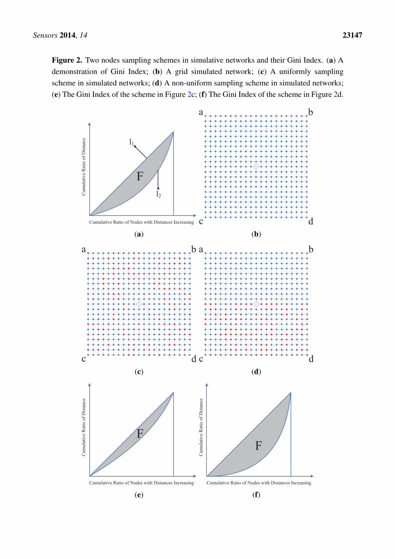
Gini index is often used for evaluating data inequality according to frequency distributions.There is a demonstration of Gini Index shown in Figure 2a, where l1 represents the perfectequal cumulative ratio, l2 represents the actual cumulative ratio, and the area of shaded partF represents the Gini Index. If l2 got closer to l1, the area of F , the Gini Index, will getsmaller. In our method, given the sampling nodes number n (determined by the sampling rate)of one data collection round, the node sampling scheme can be denoted by a binary vectorq = (q1, ..., qN)

T , which is a column of Q in Equation (2), where qi = 1 representing the ith nodeis selected for sensing data and

∑Ni=1 qi = n. For each unselected node in the network, we denote the

distance of the node to its nearest selected node by dj . Then we sort the distances and get an ascendingsequence d1 ≤ d2 ≤ ... ≤ dN−n. From the sequence, we define the evenness measurement for thedesired random sampling scheme by Gini Index in the following form:

G1(q) = 1− 1

N − n(2

N−n∑j=1

d′j − 1). (16)

where d′j =∑j

k=1 dk∑N−ni=1 di

is the cumulative ratio of distances. By minimization of G1(q), we obtain theoptimized q representing the best spatial uniform node selection scheme. As the distances among nodesare unknown for a practical network, we use the spatial correlation weights in Equation (10) to replacethe distances dj and compute the G1(q) in Equation (16). We give a concrete example. As shown inFigure 2. Figure 2b shows a simulated grid network with 21× 21 node, and Figure 2c,d show two nodesampling schemes in the simulated grid network, where the red nodes represent the nodes selected forsensing data. Figure 2e and Figure 2f show their Gini Index of Figure 2c and Figure 2d respectively.Apparently, the area of F in Figure 2e is much smaller than the one in Figure 2f as the distribution ofthe selected nodes in Figure 2c is more uniform than it in Figure 2d. So from the measurement of GiniIndex, we could obtain the optimized nodes sampling scheme.

Sensors 2014, 14 23147

Figure 2. Two nodes sampling schemes in simulative networks and their Gini Index. (a) Ademonstration of Gini Index; (b) A grid simulated network; (c) A uniformly samplingscheme in simulated networks; (d) A non-uniform sampling scheme in simulated networks;(e) The Gini Index of the scheme in Figure 2c; (f) The Gini Index of the scheme in Figure 2d.

Cumulative Ratio of Nodes with Distances Increasing

Cu

mu

lati

ve

Rat

io o

f D

ista

nce

(a) (b)

(c) (d)

Cumulative Ratio of Nodes with Distances Increasing

Cu

mu

lati

ve

Rat

io o

f D

ista

nce

(e)

Cumulative Ratio of Nodes with Distances Increasing

Cu

mu

lati

ve

Rat

io o

f D

ista

nce

(f)

Sensors 2014, 14 23148

Implementing the data collection round given the node sampling scheme q, the energy consumptionin the data sensing and delivering will result in a new energy status for the network. We denote theremaining energy of each node by ei, i = 1, ..., N . They also are sorted as an ascending sequencee1 ≤ e2 ≤ ... ≤ eN . Similarly, we define the measurements for the network energy balance by GiniIndex in the following form:

G2(q) = 1− 1

N(2

N∑i=1

e′i − 1). (17)

where e′i =∑i

k=1 ek∑Nj=1 ej

.

From Equations (16) and (17), we get a multi-objective 0-1 programming model to search the energyefficient node sampling q as the following form:

min Z = {G1(q), G2(q)}, s.t. 1Tq = n. (18)

This is a non-linear optimization problem. Considering the computation restriction in WSNs, we usethe intelligent optimization method, Particle Swarm Optimization (PSO) [36], to solve this optimizationmodel. Once obtaining the optimized node sampling scheme q, we can implement the current datacollection round and so repeat the procedure getting continuous sensing data for low rank recovery atthe sink node.

6. Experiments and Results

To evaluate the proposed method, we conduct data collection and data recovery experiments on botha simulated network and a real wireless sensor network and compare our method with other relevantmethods. In this section, we first give the experiments setup and then report the experimental results.

6.1. Experiment Environments and Parameter Setting

6.1.1. The Structure of the Simulated and Real Networks

The simulated network is a regular 21× 21 grid network, and the center node is set as the sink node,shown in Figure 2a. In the simulated network, the physical quantities can be accurately sensed andcompared with the recovered data, so the proposed method can be evaluated confidently. The real datacollection scenario is the wireless network of Intel Berkeley Research Lab [37], which has 54 nodes andthe 5th node is the sink node, shown in Figure 3. The sensing data of the real network include severalphysical quantities, such as temperature, humidity and illumination, etc. The data were collected overseveral months with a sensing time slot of half minute.

Sensors 2014, 14 23149

Figure 3. The wireless network of Intel Berkeley Research Lab [37].

6.1.2. The MAC Protocol and Routing of the Simulated and Real Networks

To the regular grid of the simulated network, the experiments are implemented on a scheduledmedium access control (MAC). Specifically, IEEE 802.15.4 is adopted as the MAC protocol. The datatransmission rate is set 250 kbps. To the nodes irregularly deployed in the real network, the experimentsare constructed with 433 MHz mica2dot nodes which adopt the default CSMA based B-MAC as theMAC layer protocol.

To model the sensing data delivering procedure, we adopt a simple routing method to transport asensing packet from a node to the sink node, in which a node selects the one-hop adjacent node withmaximal remaining energy to transmit the sensing packet. In the simulated network, the one-hop adjacentnodes of a node are the directly linked nodes in the grid. In the real networks, we set a maximal distancefor a node to transmit data package to others in one-hop. In our experiments, the upper bound is assignedto 10 m. Under this setting, we obtain the connection of the nodes in the real network. For example, theone-hop links from node 1 are shown as the arrowed lines in Figure 3.

6.1.3. The Energy Consumption Model of the Simulated and Real Networks

To evaluate the energy consumption of the network, we adopt the energy consumption model in [38]in our experiments, in which the node transmitting and reception energy consumption ETx(d) and ERx

are defined as follows:

ETx(d) = El + εad2. (19)

ERx = El. (20)

where d is the transmitting distance, El is the energy consumed of radio electronics, εa is the poweramplifier. In our experiments, all nodes are initialized with 2 × 104J of energy and the parametersEl = 50nJ/bit, εa = 10pJ/bit/m2. The sensing packet is assumed to be a fixed size of 1000 bits.

Based on the above energy consumption model, given a node sampling rate, the network lifetime isdefined as the maximal data collection rounds if the network energy can ensure the sensing data beingtransferred to the sink node.

Sensors 2014, 14 23150

6.1.4. Data Recovery Parameters Setup

In the simulated network, to simulate the change of a physical quantity, such as temperature, we usefour curves, shown as Figure 4, to represent the sensing data during a period of time corresponding tothe four corner nodes in Figure 2a. The sensing data of other nodes are then generated by the bilinearinterpolation method. A snap of the simulated measurements of the 21× 21 grid is shown in Figure 5a.These clean sensing data are regarded as the ground truth of the physical quantity. However, the realsensing data usually have some noise, so we add Gaussian noise into the clean sensing data to simulateactual measurement data, shown as Figure 5b. To form the measurement matrix X for data recovery, hereX is set as a square matrix with dimension of (21× 21− 1)× 440, i.e., N = T = 440. The parametersin Equations (9), (10) and (15) are empirically set as: λ1 = λ2 = 0.01, λ3 = 10, α = 0.1, ε = 10−5.

In the real network, the temperature sensing data collected on 53 nodes at March 1st 2004 are usedas the measurement data which has dimension of 53 × 2880. As there exist large difference for thedimensions of the row and column, we segment the measurement data into 48 blocks, where eachblock has same dimension of 53 × 60. One sample of these block is shown in Figure 6a. In the datarecovery experiments, each block is assigned as the measurements matrix X, i.e., N = 53, T = 60. Theparameters in Equations (9), (10) and (15) are set as: λ1 = λ2 = 0.01, λ3 = 10, α = 0.1, ε = 10−5. Thewhole recovered data can be obtained by stacking all the recovered blocks.

Figure 4. The simulated sensing data of four corner nodes a, b, c, d of the simulated networkin Figure 2a.

0 100 200 300 400 50016

18

20

22

24

26

28

30

32

34

Time Slot

Tem

pera

ture

(a)

0 100 200 300 400 50016

18

20

22

24

26

28

30

32

34

Time Slot

Tem

pera

ture

(b)

0 100 200 300 400 50016

18

20

22

24

26

28

30

32

34

Time Slot

Tem

pera

ture

(c)

0 100 200 300 400 50016

18

20

22

24

26

28

30

32

34

Time Slot

Te

mp

era

ture

(d)

Sensors 2014, 14 23151

Figure 5. A snap of the sensing data of the simulated network. (a) The clean sensing data;(b) The sensing data with noise.

05

1015

2025 0

10

20

30

22

23

24

25

26

27

28

Node IndexNode Index

Tem

pera

ture

(a)

05

1015

2025 0

10

20

30

22

23

24

25

26

27

28

Node IndexNode Index

Tem

pera

ture

(b)

Figure 6. The temperature sensing data from Intel Berkeley Research Lab: (a) The actualsensing data; (b) The filtered sensing data.

020

4060

80

0

20

40

6015

20

25

30

Time SlotNode Index

Tem

pera

ture

(a)

020

4060

80

0

20

40

6015

20

25

30

Time SlotNode Index

Tem

pera

ture

(b)

To evaluate the accuracy of the recovered measurement, the recovery error is defined as the averagerelative error between the recovered data and the clean sensing data (denoted by X0) at these unknownelement with the following representation:

err =

√ ∑(i,j)∈{(i,j)|Q(i,j)=0}

(X∗(i, j)−X0(i, j))2√ ∑(i,j)∈{(i,j)|Q(i,j)=0}

(X0(i, j))2. (21)

In real networks experiments, we need real clean sensing data to verify the validity of our proposeST-LRMA method. Unfortunately, the actual sampling sensing data are always corrupted and somevalues are gone missing. The real and accurate temperature data curve should be smooth and continuous,however, the actual temperature sensing data sampled over real networks are always noisy due to onereason or another. Hence, we simply use the Median filter on the temporal direction of the measurementsas the clean sensing data to compute the error, i.e., a 1D Median filter with dimension of 5 is used on each

Sensors 2014, 14 23152

row of X. The filtered results of the measurements in Figure 6a are shown in Figure 6b. Additionally,for the 48 segmented blocks in the real network, the recovery error is defined as the mean of the recoveryerrors of the 48 blocks.

To verify the performance of the proposed method on different node sampling rate, defined as the ratioof the number of the valid elements of M to the number of the complete elements of the measurementX, the data recovery experiments are conducted with the node sampling rate changing from 5% to 95%.

The rank of the measurements matrix is an important parameter for the LRMA method. However,estimation of the rank from an incomplete matrix is an open problem. To get proper rank estimation,we implement many times data recovery experiments with different rank. In addition, the data recoveryresults are computed by the above metric. The results of simulative and real networks are shown inFigure 7. According to the results, we choose different rank for the data recovery. In the simulatednetworks, the appropriate rank is assigned to 10 according to the experimental results shown in Figure 7a.In real network, the appropriate rank is assigned to 5 according to the experimental results shown inFigure 7b.

Figure 7. The data recovery results based on different estimated rank and different samplingrate. (a) The results in the simulated network; (b) The results in the real network.

6 8 10 12 14 16 18 200.035

0.036

0.037

0.038

0.039

Esimated Rank

Re

lative

Err

or

p=20%

p=40%

p=60%

p=80%

(a)

3 4 5 6 7 8 9 100.049

0.05

0.051

0.052

0.053

Esimated Rank

Re

lative

Err

or

p=20%

p=40%

p=60%

p=80%

(b)

6.2. The Result of the ST-LRMA Based Data Recovery

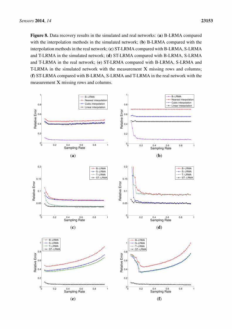
The proposed ST-LRMA based method are compared with the conventional interpolation methods(linear, cubic and nearest interpolation), the recently proposed LRMA based methods, B-LRMA [14]and T-LRMA [16], and the LRMA based method with only spatial constraint, denoted by S-LRMA.The results, shown in Figure 8a–d, indicate that the LRMA based methods have dramatic improvementin data recovery accuracy compared the conventional interpolation methods. Moreover, the proposedST-LRMA method outperforms the other LRMA based methods. Especially in the low sampling rate,the proposed method shows a more impressive superiority. This means the proposed method needs onlyfairly few measurements to obtain high data recovery accuracy. It can be regarded as an energy efficientdata collection method and this can be also proved by the following optimized sampling data collectionexperiments.

Sensors 2014, 14 23153

Figure 8. Data recovery results in the simulated and real networks: (a) B-LRMA comparedwith the interpolation methods in the simulated network; (b) B-LRMA compared with theinterpolation methods in the real network; (c) ST-LRMA compared with B-LRMA, S-LRMAand T-LRMA in the simulated network; (d) ST-LRMA compared with B-LRMA, S-LRMAand T-LRMA in the real network; (e) ST-LRMA compared with B-LRMA, S-LRMA andT-LRMA in the simulated network with the measurement X missing rows and columns;(f) ST-LRMA compared with B-LRMA, S-LRMA and T-LRMA in the real network with themeasurement X missing rows and columns.

0 0.2 0.4 0.6 0.8 10

0.2

0.4

0.6

0.8

1

Sampling Rate

Rela

tive E

rror

B−LRMA

Nearest interpolation

Cubic interpolation

Linear interpolation

(a)

0 0.2 0.4 0.6 0.8 10

0.2

0.4

0.6

0.8

1

Sampling Rate

Re

lative

Err

or

B−LRMA

Nearest interpolation

Cubic interpolation

Linear interpolation

(b)

0 0.2 0.4 0.6 0.8 10

0.05

0.1

0.15

0.2

Sampling Rate

Re

lative

Err

or

B−LRMA

S−LRMA

T−LRMA

ST−LRMA

(c)

0 0.2 0.4 0.6 0.8 10

0.05

0.1

0.15

0.2

Sampling Rate

Re

lative

Err

or

B−LRMA

S−LRMA

T−LRMA

ST−LRMA

(d)

0 0.2 0.4 0.6 0.8 10

0.2

0.4

0.6

0.8

1

Sampling Rate

Rela

tive E

rror

B−LRMA

S−LRMA

T−LRMA

ST−LRMA

(e)

0 0.2 0.4 0.6 0.8 10

0.2

0.4

0.6

0.8

1

Sampling Rate

Re

lative

Err

or

B−LRMA

S−LRMA

T−LRMA

ST−LRMA

(f)

Sensors 2014, 14 23154

According to the low rank completion theory [13], to recover a complete matrix, there should be atleast one valid entry at each row and column. However, the data loss often occurs in WSNs. So thiscondition for the LRMA model may not be guaranteed at some data measurements. To further test therobust of the proposed method, we implement the data recovery experiments with element lost in entirerows and columns of the measurement matrix. Here we randomly remove 10% of rows and columnsfrom the measurement matrices X both in the simulated and real networks. Then the above data recoveryexperiments are repeated using the new inputs. The experimental results, shown in Figure 8e,f, show theproposed ST-LRMA has stable recovery results, while B-LRMA, S-LRMA and T-LRMA generate largeerror and their curves behave un-convergently. It is considered that the improved stability of the proposedmethod is due to the newly introduced consistency constraints over measurements.

6.3. The Result of the Optimized Sampling for Energy Efficient Data Collection

Figure 9. The optimized node sampling method compared with random sampling method.(a) The network lifetime of the two sampling methods with different sampling rates in thesimulated network; (b) The network lifetime of the two sampling methods with differentsampling rates in the real network; (c) The data recovery error of the two sampling methodswith different sampling rates in the simulated network; (d) The data recovery error of thetwo sampling methods with different sampling rates in the real network.

0.1 0.2 0.3 0.4 0.5 0.6 0.7 0.8 0.94

5

6

7

8

9

10

11

12

13

14x 10

4

Sampling Rate

Ro

un

d N

um

be

r

Random sampling

Optimized sampling

(a)

0.1 0.2 0.3 0.4 0.5 0.6 0.7 0.8 0.93

4

5

6

7

8

9

10

11

12x 10

5

Sampling Rate

Ro

un

d N

um

be

r

Random sampling

Optimized sampling

(b)

0.1 0.2 0.3 0.4 0.5 0.6 0.7 0.8 0.95.4

5.5

5.6

5.7

5.8

5.9

6

6.1

6.2

Sampling Rate

Re

lative

Err

or

Random Sampling

Opitimized Sampling

x 10−2

(c)

0.1 0.2 0.3 0.4 0.5 0.6 0.7 0.8 0.93.6

3.7

3.8

3.9

4.0

4.1

4.2

4.3

4.4

4.5

4.6

Sampling Rate

Re

lative

Err

or

Random sampling

Optimized sampling

x 10−2

(d)

Sensors 2014, 14 23155

To evaluate performance of the optimized node sampling method, we implement data collection inthe whole network lifetime with different node sampling rate. The results are compared with the randomsampling method, as shown in Figure 9a for the simulated network and Figure 9b for the real network,respectively. It is shown that the optimized node sampling method has better performance than therandom sampling method for both the simulated and real networks. Especially in the lower samplingrate, the optimized node sampling method could obtain better network energy distribution and prolongthe network lifetime. For example, when the sampling rate is lower than 30%, the network lifetime ofthe optimized method will be prolonged two times than the network lifetime of the random method.

The data recovery errors are also computed for the two node sampling methods and the results arereported in Figure 9c,d. In the simulated network or the real network, the optimized node samplingmethod almost has the same performance to the ideal random sampling method which is consideredthe best way to get good recovery results. From these, we can conclude that the optimized method cannot only extend the network lifetime but also keep the accuracy of the data recovery. This is due tothe balanced model concerning the node uniform sampling and the energy distribution of network inSection 5.

7. Conclusion

In this paper, we propose an efficient data collection method based on LRMA for WSNs. Thecontribution of the work lies in two folds. On one hand, a proposed novel ST-LRMA baseddata collection method introduces the spatial and temporal correlation of the sensing data into theconventional LRMA model. The experiment results indicate that the proposed method has better datarecovery accuracy compared with the conventional interpolation methods and the state-of-the-art LRMAbased methods. In addition, the proposed method avoids the optimization problem involving emptycolumns or rows, and could fill the empty columns or rows stably. On the other hand, an optimizednodes sampling method is proposed and integrated with the ST-LRMA based data collection method.In the proposed nodes sampling model, Gini index is adopted to measure the uniformity of the selectednodes and the distribution of the network energy. The data collection experiments were conducted onthe simulated and real wireless networks. The results show the proposed method has good performanceon network energy efficiency without losing much data recovery accuracy.

Our experiments are implemented without considering some network properties, such as the complexrouting, the network time duty circle, and the sensing data attributes. The future work is to integratethese network properties into our ST-LRMA based data collection method and apply it on real largescale wireless sensor networks. Another possible future work is to consider the multi-modality sensingdata together and to formulate the sensing data as tensors to be recovered by low rank alike constraints.

Acknowledgments

This paper is supported by National Natural Science Foundation of China Grants (No. 61390510,61133003, 61370119 and 61171169); The Australian Research Council (ARC) through a DiscoveryProject (DP) grant (DP140102270); Beijing Natural Science Foundation Grants (No. 4132013,KZ201310005006 and PHR(IHLB)).

Sensors 2014, 14 23156

Author Contributions

This paper presents part of Xinglin Piao Ph.D. study research. Yongli Hu designed the research,drafted the manuscript and contributed to carrying out the experiment and performing the data analysis.Yanfeng Sun, Baocai Yin and Junbin Gao contributed with valuable discussions and scientific advice.All authors read and approved the final manuscript.

Conflicts of Interest

The authors declare no conflict of interest.

References

1. Li, M.; Liu, Y. Underground coal mine monitoring with wireless sensor networks. ACM Trans.Sens. Netw. 2009, 5, 1–29.

2. Vuran, M.C.; Akan, O.B.; Akyildiz, I.F. Spatio-temporal correlation: Theory and applications forwireless sensor networks. Comput. Netw. J. 2004, 45, 245–259.

3. Hua, G.; Chen, C. Correlated data gathering in wireless sensor networks based on distributed sourcecoding. Int. J. Sens. Netw. 2008, 4, 13–22.

4. Jim, C.; Petrovic, D.; Ramachandran, K. A distributed and adaptive signal processing approachto reducing energy consumption in sensor networks. In Proceedings of Twenty-Second AnnualJoint Conference of the IEEE Computer and Communications, San Francisco, CA, USA,30 March–3 April 2003; pp. 1054–1062.

5. Yuen, K.; Liang, B.; Li, B. A distributed framework for correlated data gathering in sensornetworks. IEEE Trans. Veh. Technol. 2008, 57, 578–593.

6. Ciancio, A.; Pattem, S.; Ortega, A.; Krishnamachari, B. Energy efficient data representation androuting for wireless sensor networks based on a distributed wavelet compression algorithm. InProceedings of the Fifth International Conference on Information Processing in Sensor Networks,Nashville, TN, USA, 19–21 April 2006; pp. 309–316.

7. Crovella, M.; Kolaczyk, E. Graph wavelets for spatial traffic analysis. In Proceedingsof Twenty-Second Annual Joint Conference of the IEEE Computer and Communications,San Francisco, CA, USA, 30 March–3 April 2003; pp. 1848–1857.

8. Yoon, S.; Shahabi, C. The clustered aggregation (cag) technique leveraging spatial and temporalcorrelations in wireless sensor networks. ACM Trans. Sens. Netw. 2007, 3, 1–39.

9. Liu, C.; Wu, K.; Pei, J. An energy-efficient data collection framework for wireless sensor networksby exploiting spatiotemporal correlation. IEEE Trans. Parallel Distrib. Syst. 2007, 18, 1010–1023.

10. Gupta, H.; Navda, V.; Das, S.; Chowdhary, V. Efficient gathering of correlated data in sensornetworks. ACM Trans. Sens. Netw. 2005, 3, 31–43.

11. Xu, X.; Li, X.; Wan, P.; Tang, S. Efficient scheduling for periodic aggregation queries in multihopsensor networks. IEEE/ACM Trans. Netw. 2012, 20, 690–698.

12. Recht, B.; Fazel, M.; Parrilo, P. Guaranteed Minimum-Rank Solutions of Linear Matrix Equationsvia Nuclear Norm Minimization. SIAM Rev. 2010, 52, 471–501.

Sensors 2014, 14 23157

13. Candès, E; Recht, B. Exact Matrix Completion via Convex Optimization. Found. Comput. Math.2009, 9, 717–772.

14. Cheng, J.; Jiang, H.; Ma, X.; Liu, L.; Qian, L.; Tian, C.; Liu, W. Efficient Data Collection withSampling in WSNs: Making Use of Matrix Completion Techniques. In Proceedings of IEEEGlobal Telecommunications Conference, Miami, FL, USA, 6–10 December 2010; pp. 1–5.

15. Cheng, J.; Ye, Q.; Jiang, H.; Wang, D.; Wang, C. STCDG: An efficient data gathering algorithmbased on matrix completion for wireless sensor networks. IEEE Trans. Wirel. Commun. 2013, 12,850–861.

16. Piao, X.; Hu, Y.; Sun, Y.; Yin, B. Efficient Data Gathering in Wireless Sensor Networks Based onLow Rank Approximation. In Proceedings of IEEE International Conference on and IEEE Cyber,Physical and Social Computing, Green Computing and Communications (GreenCom), 2013 IEEEand Internet of Things (iThings/CPSCom), Beijing, China, 20–23 August 2013; pp. 699–706.

17. Mainwaring, A.; Culler, D.; Polastre, J.; Szewczyk, R.; Anderson, J. Wireless sensor networks forhabitat monitoring. In Proceedings of The First ACM International Workshop on Wireless SensorNetworks and Applications, Atlanta, GA, USA, 28 September 2002; pp. 88–97.

18. Luo, C.; Wu, F.; Sun. J.; Chen, C. Compressive data gathering for large-scale wireless sensornetworks. In Proceedings of The Fifteenth Annual International Conference on Mobile Computingand Networking, Beijing, China, 20–25 September 2009; pp. 145–156.

19. Chou, C.; Rana, R.; Hu, W. Energy efficient information collection in wireless sensor networksusing adaptive compressive sensing. In Proceedings of IEEE Thirty-fourth Conference on LocalComputer Networks, Zurich, Switzerland, 20–23 October 2009; pp. 443–450.

20. Xiang, L.; Luo, J.; Vasilakos, A. Compressed data aggregation for energy efficient wirelesssensor networks. In Proceedings of Eighth Annual IEEE Communications Society Conferenceon Sensor, Mesh and Ad Hoc Communications and Networks (SECON), Salt Lake City, UT, USA,27–30 June 2011; pp. 46–54.

21. Xiang, L.; Luo, J.; Rosenberg, C. Compressed data aggregation: Energy-efficient and high-fidelitydata collection. IEEE/ACM Trans. Netw. 2013, 21, 1722–1735.

22. Wu, X.; Xiong, Y.; Huang, W.; Shen, H.; Li, M. An efficient compressive data gathering routingscheme for large-scale wireless sensor networks. Comput. Electr. Eng. 2013, 39, 1935–1946.

23. Bajwa, W.; Haupt, J.; Sayeed, A.; Nowak, R. Compressive wireless sensing. In Proceedings ofthe Fifth International Conference on Information Processing in Sensor Networks, Nashville, TN,USA, 19–21 April 2006; pp. 134–142.

24. Haupt, J.; Bajwa, W.; Rabbat, M.; Nowak, R. Compressed sensing for networked data. IEEE SignalProcess. Mag. 2008, 25, 92–101.

25. Lin, Z.; Ganesh, A.; Wright, J.; Wu, L.; Chen, M.; Ma, Y. Fast convex optimization algorithms forexact recovery of a corrupted low-rank matrix. In Proceedings of the Third International Workshopon Computational Advances in Multi-Sensor Adaptive Processing, Aruba, The Netherlands,13–16 December 2009; pp. 213–216.

26. Zhang, Y.; Roughan, M.; Willinger, W.; Qiu, L. Spatio-temporal compressive sensing and internettraffic matrices. In Proceedings of the Ninth ACM SIGCOM, Barcelona, Spain, 17–21 August2009; pp. 267–278.

Sensors 2014, 14 23158

27. Nikitaki, S.; Tsagkatakis, G.; Tsakalides, P. Efficient training for fingerprint based positioningusing matrix completion. In Proceedings of the Twentieth European Signal Processing Conference(EUSIPCO), Bucharest, Rumania, 27–31 August 2012; pp. 195–199.

28. Hu, Y.; Zhou, W.; Wen, Z.; Sun, Y.; Yin, B. Efficient Radio Map Construction Based on Low-RankApproximation for Indoor Positioning. J. Math. Probl. Eng. 2013, 2013, No. 461089.

29. Tibshirani, R.; Saunders, M.; Rosset, S.; Zhu, J.; Knight, K. Sparsity and smoothness via the fusedlasso. J. Roy. Stat. Soc. B 2005, 67, 91–108.

30. Guo, Y.; Gao, J.; Li, F. Spatial Subspace Clustering for Drill Hope Spectral Data. J. Appl. RemoteSens. 2014, 8, 1–9.

31. Tierney, S.; Gao, J.; Guo, Y. Subspace Clustering for Sequential Data. In Proceedings of 2014IEEE Conference on Computer Vision and Pattern Recognition, Columbus, OH, USA, 23–28 June2014; 1019–1026.

32. Roweis, S.; Saul, L. Nonlinear dimensionality reduction by locally linear embedding. Science2000, 290, 2323–2326.

33. Tenenbaum, J.B.; Silva, V.; Langford, J.C. A global geometric framework for nonlineardimensionality reduction. Science 2000, 290, 2319–2323.

34. Belkin, M.; Niyogi, P.; Dietterich, T.G.; Becker, S.; Ghahramani, Z. Laplacian eigenmaps andspectral techniques for embedding and clustering. In Proceedings of Fifteenth Annual Conferenceon Neural Information Processing Systems, Vancouver, BC, Canada, 3–8 December 2001;pp. 585–591.

35. Elhamifar, E.; Vidal, R. Sparse manifold clustering and embedding. In Proceedings ofTwenty-Fifth Annual Conference on Neural Information Processing Systems, Granada, Andalusia,Spain, 12 December 2011; pp. 55–63.

36. Kennedy. J.; Eberhart, R. Particle Swarm Optimization. In Proceedings of IEEEInternational Conference on Neural Networks, Perth, Australia, 27 November–1 December 1995;pp. 1942–1948.

37. Intel Lab Data. Available online: http:// db.csail.mit.edu/labdata/labdata.html (accessed on 16September 2014).

38. Tian, D.; Georganas, N.D. A node scheduling scheme for energy conservation in large wirelesssensor networks. Wirel. Commun. Mob. Comput. 2003, 3, 271–290.

c© 2014 by the authors; licensee MDPI, Basel, Switzerland. This article is an open access articledistributed under the terms and conditions of the Creative Commons Attribution license(http://creativecommons.org/licenses/by/4.0/).