SensorFlock: An Airborne Wireless Sensor Network of Micro-AirVehicles∗

1Jude Allred, 1Ahmad Bilal Hasan, 1Saroch Panichsakul, 2William Pisano,2Peter Gray, 1Jyh Huang,1Richard Han, 2Dale Lawrence, 2Kamran Mohseni

1Department of Computer Science, University of Colorado, Boulder.2Department of Aerospace Engineering Sciences, University of Colorado, Boulder.

{Saroch.Panichsakul, William.Pisano}@colorado.edu

AbstractAn airborne wireless sensor network (WSN) composed

of bird-sized micro aerial vehicles (MAVs) enables low costhigh granularity atmospheric sensing of toxic plume be-havior and storm dynamics, and provides a unique three-dimensional vantage for monitoring wildlife and ecologicalsystems. This paper describes a complete implementation ofour SensorFlock airborne WSN, spanning the developmentof our MAV airplane, its avionics, semi-autonomous flightcontrol software, launch system, flock control algorithm, andwireless communication networking between MAVs. Wepresent experimental results from flight tests of flocks ofMAVs, and a characterization of wireless RF behavior in air-to-air communication as well as air-to-ground communica-tion.

Categories and Subject DescriptorsJ.2 [Computer Applications]: Physical Sciences and En-

gineering—Earth and atmospheric sciences; C.2.1 [Compu-ter-Communication Networks]: Network Architecture andDesign—Wireless Communications

General TermsMeasurement, Performance, Design, Experimentation

KeywordsWireless Sensor Networks, MAVs, Applications, Deploy-

ments

∗This work was supported by the National Science Foundation(NSF) project: ITR: Loosely Cooperating Micro Air Vehicle Net-works for Toxic Plume Characterization (grant number 0427947)

Permission to make digital or hard copies of all or part of this work for personal orclassroom use is granted without fee provided that copies are not made or distributedfor profit or commercial advantage and that copies bear this notice and the full citationon the first page. To copy otherwise, to republish, to post on servers or to redistributeto lists, requires prior specific permission and/or a fee.SenSys’07, November 6–9, 2007, Sydney, Australia.Copyright 2007 ACM 1-59593-763-6/07/0011 ...$5.00

1 IntroductionLarge wireless networks scaling to hundreds of low cost

airborne vehicles are largely still a vision today rather than areality. In our SensorFlock airborne wireless sensor network(WSN), our research goal is to make a substantial leap for-wards towards this vision of hundreds of inexpensive, semi-autonomous, and cooperating airborne vehicles that senseand relay data over a wireless communication mesh net-work. We present in this paper our progress towards thisgoal, namely the design of our micro-air vehicle (MAV), thesemi-autonomous flight control algorithm capable of hover-ing individual MAVs in loiter circles, flight validation tests ofthe MAVs, and an in-depth study of the RF characteristics ofair-to-air and air-to-ground communication between MAVs.The benefits that will accrue to the research community fromthe SensorFlock project include the ability to enhance sci-entific applications with fine-granularity three-dimensionalsampling, the distribution of the MAV aircraft design andsoftware to the wider community, the eventual creation ofairborne testbeds that scale up to hundreds of MAVs, andincreased understanding of wireless propagation character-istics and networking connectivity behavior between largenumbers of MAVs that are rapidly banking and rolling inflight. The latter measurement results will aid the computerscience community in developing more realistic RF modelsfor in situ air-to-air and air-to-ground communication, thusleading to improved simulation and design of more robustprotocols for practical airborne sensor networks.

An airborne WSN provides the capability to enhancemany applications of interest to the scientific communityby providing finer granularity three-dimensional samplingof phenomena of interest than would otherwise be feasible.One such class of applications is chemical dispersion sam-pling. As shown in Figure 1, a deployment of a flock ofMAVs sensing and communicating their data back to a net-work of ground stations enables scientists to study the rateof dispersion of a toxin, pollutant, or chemical, natural orman-made. In another example, MAV flocks may providethe ability to study the distribution of CO2 concentrationsin the atmosphere and its relation to global warming. In allthese cases, a flock of MAVs enables accurate sampling of

Figure 1. An airborne WSN for 3-D sensing of toxicplumes.

the parameter of interest simultaneously over large regionsof a volume. In addition, since MAVs are independentlycontrollable, they can be targeted to track the toxic plumeto study the rate of dispersion, fly towards the source of theplume if unknown, and re-distribute to map the boundariesof the plume.

Another class of applications that would benefit from anairborne WSN are those involving atmospheric weather sens-ing. A flock of MAVs - each MAV equipped with tempera-ture, pressure, humidity, wind speed/direction, and/or othersensors - can provide detailed in-situ mapping of weatherphenomena such as hurricanes, thunderstorms, and torna-dos, and return data that would be useful in improving stormtrack predictions and the understanding of storm genesis andevolution. Other such examples include: modeling the localweather produced by wildfires to better predict their evolu-tion and improve the deployment of firefighting resources;sensing and modeling of thermodynamic plumes over openice leads in polar regions to better understand interactions be-tween sea, ice, and atmosphere which contribute to climatechange; and improved characterization of heat islands abovecities and their impact on local weather patterns.

While many technologies exist that can contribute to theairborne WSN vision, they are either too costly, too re-stricted, or too limited to fully achieve by themselves a lowcost and retargetable airborne sensor network. Passive sen-sors such as weather balloons and dropsondes cannot be re-targeted to phenomena of interest. Large Unmanned Air Ve-hicles (UAVs) of 2-3 meter wingspan or more pose a hazardto conventional air traffic and ground personnel. Small, birdsized sensor vehicles have the potential to reduce the conse-quences of failure to levels that are considered of equivalentsafety to FAA approved manned vehicles.

We have therefore pursued a vision of building an air-borne WSN composed of many low cost small bird-sizedMAVs on the order of a half a meter in wingspan. An ex-ample of the MAV that we have built is shown in Figure 2.This MAV would pose little danger to personnel and propertyon the ground or other air vehicles. They do not need spe-cialized take-off or landing facilities or runways. They arereusable, and could be produced in large numbers at low cost.With a few enhancements to our current prototype’s airframeand propulsion system, such small vehicles could potentiallyremain in flight for periods of about 90 minutes, sufficientto provide highly accurate data for decisions in the critical

Figure 2. Micro Air Vehicle (MAV) designed and built forflight tests of our airborne WSN.

initial period after a toxin release event. Subsequently, fewernumbers might be used to monitor dispersions over longerperiods.

Deploying an airborne WSN with large numbers of vehi-cles (e.g. tens or hundreds) raises unique research challengesin command and control. Each MAV carries very limited on-board power and computing resources. Flight control, toxinsensing, information processing, communication, and deci-sion making must be extremely simple and decentralized.Yet rather sophisticated aggregate behavior is desired, so thatthe flock can semi-autonomously seek out plumes, guided bysupervisory human operators and real-time models of plumeevolution.

This paper describes our SensorFlock solution to large-volume atmospheric sensing, that takes the approach of us-ing a ”minimal” autopilot combined with a globally stableand convergent vector field guidance system on each vehicle.This provides a small, low mass, and low cost autopilot sys-tem that requires very little human interaction in the form offlight control or path planning. This combination provides asemi-autonomous capability for each MAV, where the opera-tor or an overseeing algorithm can provide the desired centerof loiter coordinates and a loiter radius infrequently, decen-tralizing the vehicle control by moving the management ofthe flock to a higher level in the control hierarchy. Once theplane reaches its destination it will fly loiter circles aroundthe target point until it is told to do otherwise. With this ap-proach many vehicles can be controlled by a single operatorwithout the threat of failure due to a lack of command orloss of communication. In this manner, the airborne WSNcan scale to large number of MAVs launched and overseenby a small number of human operators. The sections belowdescribe how this system is implemented and show experi-mental results of the system in action.

2 Related WorkDetailed measurements of wireless behavior are essen-

tial to understanding real-world performance of wireless net-works. For 802.11 2.4 GHz networks, measurements havebeen performed on static WiFi LANs [1, 4, 2, 9, 8], and an

entire workshop has been devoted to the topic [10]. Mobilevehicular 802.11 ground networks have recently been stud-ied [7].

In wireless sensor networks, detailed measurements havebeen performed on testbeds of static wireless motes at900 MHz [11, 27, 24, 29]. Experimental papers studying802.15.4 radios at 2.4 GHz in static sensor networks havealso been reported [19, 21, 28].

Prior work has explored using large UAVs for toxin dis-persion characterization [17], though this is in simulationonly. Other prior work have simulated UAV networks [26,25, 12].

Practical airborne systems of wireless networked planesare largely in their infancy. A system with several small heli-copters has been reported [3]. The AUGNET project reportsresults for two of the larger UAVs [5, 6, 14] networked via802.11, not for the smaller bat-sized MAVs.

As far as we are aware, there is no prior work studyingthe network dynamics of an airborne WSN composed of bat-sized MAVs. MAVs have attracted significant attention sincethe mid-1990’s for both civilian and military applications.Pioneering work in this area was conducted by AeroViron-ment [13] and the University of Florida [15] among others.MAVs are by definition small (by weight or size) aircraftswhich fly at relatively low speeds. Control of such smalllightweight aircraft is especially challenging given changingwind vectors, although small birds and insects have been fly-ing under these conditions for quite some time. Our work inmanaging an airborne WSN focused on developing controlalgorithms to manage a flock of MAVs [18], wherein the lo-cation of each MAV was governed by a control law that was afunction of the sensing phenomena of interest, the concentra-tion of MAVs in a given area, communication requirements,and energy.

Cooperative control of a team of UAVs has also been in-vestigated [16]. This work explores task assignment and tra-jectory planning on real-world UAVs. The focus of the workis not on wireless characterization.

3 MAV SystemThe design of the MAV system faced three significant

challenges: building a sufficiently lightweight plane capa-ble of flight; designing algorithms into software to achievesemi-autonomous flight; and integrating disparate subsys-tems such as propulsion, flight control, and wireless net-working into a fully functional airborne WSN solution.

3.1 MAV PlaneAs shown in Figure 2, the small size of the MAVs de-

signed at the University of Colorado at Boulder has the ad-vantage that in the event of an accident, the potential fordamage to property and personnel on the ground is minimal.By keeping the vehicle mass under 500 grams and the max-imum speed, even in failure, under 20 m/s, these vehiclesfall within NASA’s ”Inert Debris” range safety classification.Adding that the plane is made of polypropylene foam, andthe propeller is in the rear, the potential for collision damageis minimal. Combine this with a production cost of the entireaircraft, including the autopilot, which is less than $600, andit is clear that the cost of failure of one of these vehicles is

Figure 3. CUPIC Autopilot board. This view shows thetop of the board which houses the CPU, pressure sensor,radio, and rate gyro. The integrated GPS receiver is onthe bottom of the board.

minimal. It is for this reason that we do not require redun-dant systems such as those present on larger aircraft autopilotsystems.

3.2 AvionicsThe CUPIC avionics board is structured around the Mi-

crochip PIC18F8722 8-bit microcontroller. The addition ofan RC class receiver for testing and fail-safe purposes, andan antenna for the GPS receiver completes the flight package.Analog flight sensors consist of a single roll rate gyro and anabsolute pressure sensor, while the GPS sends binary navi-gation information to the CPU. The control system runs onthe PIC and outputs commands to the motor and servos viathe on-board PWM interface. An XBee Pro Zigbee class 2.4GHz radio is used to support wireless communication andmobile networking. The system is capable of being flown en-tirely through the XBee, but a backup RC link is maintainedfor network testing when there is a possibility of losing con-tact with an aircraft.

3.3 Fail-safe OperationAn important consideration when operating any aircraft

is concern for safety. Several fail-safes are present in theautopilot system to cope with failure contingencies in flight.A watchdog timer is present that will restart the CPU if thetimer is not periodically serviced. This avoids the case wherea software bug causes a system crash, preventing the controlsystem from executing regularly. The current setup uses twoRF links , where the second RF link is a modified Pulse CodeModulated Remote Control radio, commonly used in the RCmodeling community. The range of this radio is approxi-mately 1.5 kilometers. Current operating procedure dictatesthat the aircraft be within visual range at all times. Visualrange is about 1/2 kilometer, which is much less than therange of the radio, thus loss of contact due to range shouldnot be an issue. In the potential case where the plane startsflying away from the operator, there is a fail-safe in placethat will turn the motor off when the plane loses the RC link.With the motor off, the aircraft will gently glide down.

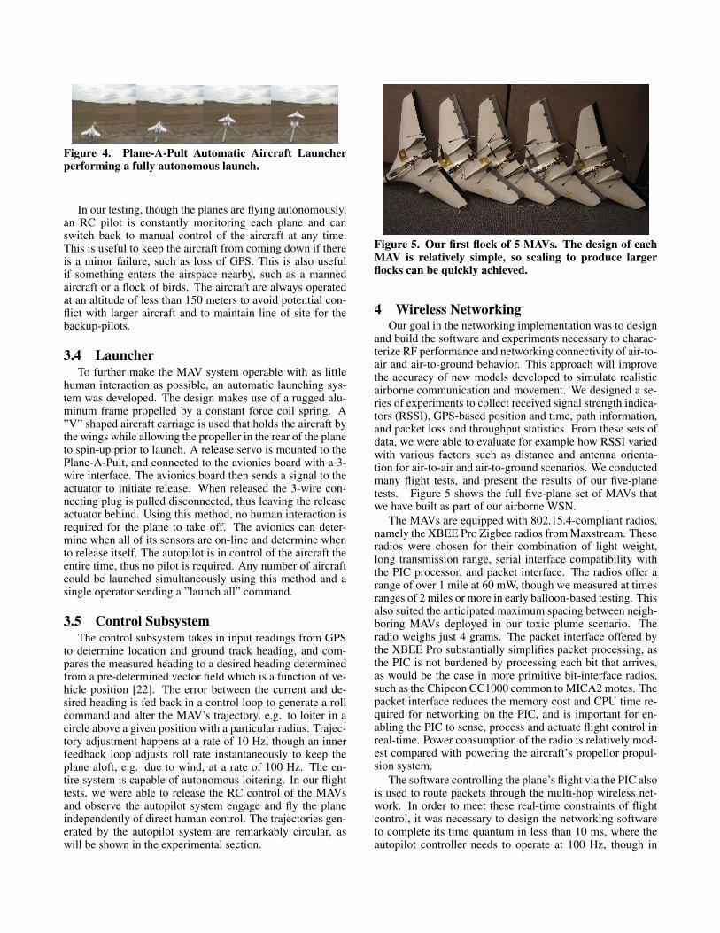
Figure 4. Plane-A-Pult Automatic Aircraft Launcherperforming a fully autonomous launch.

In our testing, though the planes are flying autonomously,an RC pilot is constantly monitoring each plane and canswitch back to manual control of the aircraft at any time.This is useful to keep the aircraft from coming down if thereis a minor failure, such as loss of GPS. This is also usefulif something enters the airspace nearby, such as a mannedaircraft or a flock of birds. The aircraft are always operatedat an altitude of less than 150 meters to avoid potential con-flict with larger aircraft and to maintain line of site for thebackup-pilots.

3.4 LauncherTo further make the MAV system operable with as little

human interaction as possible, an automatic launching sys-tem was developed. The design makes use of a rugged alu-minum frame propelled by a constant force coil spring. A”V” shaped aircraft carriage is used that holds the aircraft bythe wings while allowing the propeller in the rear of the planeto spin-up prior to launch. A release servo is mounted to thePlane-A-Pult, and connected to the avionics board with a 3-wire interface. The avionics board then sends a signal to theactuator to initiate release. When released the 3-wire con-necting plug is pulled disconnected, thus leaving the releaseactuator behind. Using this method, no human interaction isrequired for the plane to take off. The avionics can deter-mine when all of its sensors are on-line and determine whento release itself. The autopilot is in control of the aircraft theentire time, thus no pilot is required. Any number of aircraftcould be launched simultaneously using this method and asingle operator sending a ”launch all” command.

3.5 Control SubsystemThe control subsystem takes in input readings from GPS

to determine location and ground track heading, and com-pares the measured heading to a desired heading determinedfrom a pre-determined vector field which is a function of ve-hicle position [22]. The error between the current and de-sired heading is fed back in a control loop to generate a rollcommand and alter the MAV’s trajectory, e.g. to loiter in acircle above a given position with a particular radius. Trajec-tory adjustment happens at a rate of 10 Hz, though an innerfeedback loop adjusts roll rate instantaneously to keep theplane aloft, e.g. due to wind, at a rate of 100 Hz. The en-tire system is capable of autonomous loitering. In our flighttests, we were able to release the RC control of the MAVsand observe the autopilot system engage and fly the planeindependently of direct human control. The trajectories gen-erated by the autopilot system are remarkably circular, aswill be shown in the experimental section.

Figure 5. Our first flock of 5 MAVs. The design of eachMAV is relatively simple, so scaling to produce largerflocks can be quickly achieved.

4 Wireless NetworkingOur goal in the networking implementation was to design

and build the software and experiments necessary to charac-terize RF performance and networking connectivity of air-to-air and air-to-ground behavior. This approach will improvethe accuracy of new models developed to simulate realisticairborne communication and movement. We designed a se-ries of experiments to collect received signal strength indica-tors (RSSI), GPS-based position and time, path information,and packet loss and throughput statistics. From these sets ofdata, we were able to evaluate for example how RSSI variedwith various factors such as distance and antenna orienta-tion for air-to-air and air-to-ground scenarios. We conductedmany flight tests, and present the results of our five-planetests. Figure 5 shows the full five-plane set of MAVs thatwe have built as part of our airborne WSN.

The MAVs are equipped with 802.15.4-compliant radios,namely the XBEE Pro Zigbee radios from Maxstream. Theseradios were chosen for their combination of light weight,long transmission range, serial interface compatibility withthe PIC processor, and packet interface. The radios offer arange of over 1 mile at 60 mW, though we measured at timesranges of 2 miles or more in early balloon-based testing. Thisalso suited the anticipated maximum spacing between neigh-boring MAVs deployed in our toxic plume scenario. Theradio weighs just 4 grams. The packet interface offered bythe XBEE Pro substantially simplifies packet processing, asthe PIC is not burdened by processing each bit that arrives,as would be the case in more primitive bit-interface radios,such as the Chipcon CC1000 common to MICA2 motes. Thepacket interface reduces the memory cost and CPU time re-quired for networking on the PIC, and is important for en-abling the PIC to sense, process and actuate flight control inreal-time. Power consumption of the radio is relatively mod-est compared with powering the aircraft’s propellor propul-sion system.

The software controlling the plane’s flight via the PIC alsois used to route packets through the multi-hop wireless net-work. In order to meet these real-time constraints of flightcontrol, it was necessary to design the networking softwareto complete its time quantum in less than 10 ms, where theautopilot controller needs to operate at 100 Hz, though in

(a) The team preparing to fly the flock of MAVs. (b) Three MAVs in flight simultaneously.

Figure 6. Pictures of the flight tests.

reality 40 Hz should suffice. To maintain simplicity, we im-plemented a simple software control loop that first consultedthe controller and then invoked the networking subsystem,alternating between these two subsystems in an indefiniteloop. The networking code was written to quickly executein its time quantum of 10 ms, and we estimate it did not takemore than 0.5 ms in practice. Our networking code only pro-cesses one packet per invocation, so as to relinquish controlback to the autopilot as soon as possible. This constrainedthe networking code from taking over the processor. Theentire code uses about 1 KB out of the total of 4 KB RAMfor the PIC, with about 150 bytes devoted to the networking.We found that this approach was acceptable for maintainingflight while also simultaneously reporting and routing net-working data on the PIC processor.

We designed the following experiment to characterizethe wireless network to the fullest extent practicable. EachMAV periodically flooded data packets 5 times per secondthroughout the network. Zigbee routing was disabled onthe XBEE radios to permit our custom routing, though wecontinued to use the 802.15.4 MAC layer. Each data packetcontained the originating source ID, the GPS location of thesource, the GPS time, the hop count, the sequence number,and the local sender’s ID, among other fields. Each nodewould forward the data packet only if its sequence num-ber exceeded the current highest recorded sequence numberfrom the originating source. In addition, each node wouldappend its ID and the RSSI of the packet to the packet’s pay-load. This approach allowed us both to evaluate the connec-tivity of every link in the mobile network, and to trace themulti-hop paths of packets through the mobile network.

The base station collected all data packets that it receivedfrom each MAV, thus enabling a rich characterization of allpaths to the basestation, and the link strengths along the way.However, this only captures part of the behavior of the net-work, since it does not capture paths to each MAV. Sincebandwidth limitations prevented us from reporting the pathtaken by each data packet received by each MAV, as was thecase at the base station, then our approach was to have eachMAV collect aggregate statistics of paths to it and periodi-cally report summaries of network connectivity to it.

Each MAV computed aggregate statistics of the packetloss, RSSI, and hop count distribution from each of the otheroriginating sources, as well as from each of its current di-rect neighbors. Every received data packet would be usedto update the aggregate statistics, whether that packet wasforwarded or not. Aggregate source statistics and neigh-bor statistics were collected and reported separately in al-ternating non-overlapping ten second intervals. Nodes usedthe same flooding mechanism to route these statistics reportsback to the base station.

5 Wireless ExperimentsOur goal in performing flight test experiments was to de-

velop a realistic understanding of the airborne RF link’s be-havior, as well as multi-hop networking performance in sucha mobile airborne environment. We performed experimentsthat evaluated the performance of air-to-air, air-to-ground,and ground-to-ground wireless links. We present in this sec-tion detailed analyses of RSSI, path loss exponents, packetloss, symmetry, and multi-hop behavior.

The experiments were performed by flying a flock of fiveMAVs. Figure 6(a) illustrates the team preparing to fly ourflock of MAVs. Figure 6(b) shows in one frame three of theMAVs in flight. To satisfy safety concerns during our tests,each MAV had a human RC pilot acting as backup for theautonomous flight software. This logistical complication, inaddition to uncooperative weather, hardware, and softwaresystem development factors, raised significant challenges inthe collection of the data presented here.

The networking code sourced packets at a rate of 5 pack-ets/sec. Each packet contained at least the following: GPS(x,y,z) coordinates; GPS time; packet sequence number;source ID; hop count; and a field for substituting the RSSIupon reception. Application packets are of fixed length of 50bytes. In each MAV, the antenna is a quarter wave whip witha very small ground plane, so that the pattern can be approxi-mated by the donut/toroid-shaped antenna pattern of the halfwave dipole. The antenna is oriented vertically, pointing up-wards when the plane is level. Transmit power was set to thelowest value of 10 dBm. The 802.15.4 radios were config-ured for a rate of 56 kbps. API mode was enabled for the ra-dios, so that data could be sent and retrieved in a pre-defined

(a) Top view of 5 MAVs loiter circling (b) 3D view of 5 MAVs loiter circling

Figure 7. Color-coded trajectories of five-MAV flight test, including loiter circles (distances given in meters).

packet format. API mode also conveniently returns the RSSIof received packets. Packets are only returned by the radioif they pass the 802.15.4 error detection check. MAVs wereprogrammed to loiter around a chosen point with a radius of50 m. During our experiments, we verified using the WiSpyspectrum analyzer that there were no other sources of wire-less interference in our immediate area from transmitters atthe same 2.4 GHz frequency.

5.1 A Five-Plane Flight TestTo provide a sense of the dynamic behavior of MAVs

while in flight, Figure 7 shows the actual trajectories of fiveMAVs obtained from their GPS coordinates during one ofour flight tests. As the trajectories are color coded, thesefigures are best viewed on a color viewer or printout. TheMAVs were programmed to loiter over different points. Thetrajectories shown capture about 30 minutes of flight, orabout 10K packets from each MAV. The base station is lo-cated near (700,700). The MAVs were launched from a pointabout 200 m away from the base station and then flown totheir loitering point, at which point autonomous loiteringwas enabled. The farthest distance in the (x,y)-plane thata MAV flew from the base station was around 500 m. Thehighest altitude flown during the test was about 125 m.

As can be seen from Figure 7(a), the top-down view ofthe flight patterns reveals that four of the MAVs achievenearly circular loitering during part of their trajectories, con-firming that the loitering software was operating correctlywhen enabled. MAV 3 (green) was manually remote con-trolled, and was piloted for part of its flight to create somestraight line flight patterns. Figure 7(b) provides a morethree-dimensional perspective on the relative trajectory ofeach flight.

5.2 Characterization of Air-to-Air ReceivedSignal Strength

Our next step is to characterize the airborne RF link’s be-havior. In particular, we seek to understand in this section

Figure 8. Average RSSI vs. distance for air-to-air, air-to-ground, and ground-to-ground wireless links.

how air-to-air received signal strength is impacted by a va-riety of factors such as distance and antenna orientation ofboth the transmitter and receiver. After gaining an under-standing of what factors influence RSSI, we will cover in thenext subsection the behavior of packet loss.

5.2.1 Path Loss ExponentFigure 8 shows the average RSSI vs. distance for air-

to-air (AtoA), air-to-ground (AtoG), and ground-to-ground(GtoG) wireless links. The RSSI for the AtoA link falls offmore gradually with distance than GtoG links, and is simi-lar in behavior to AtoG links. We expect GtoG links to suffermore from shadowing, lack of RF line of sight, and multipaththan AtoA links, which have a direct line of sight. Also, thedeviation of RSSI for the AtoA link is substantially smallerthan the GtoG link. We believe the same ground effects men-tioned earlier will also lead to a wider variation in RSSI for

GoG links than AtoA links under similar circumstances.The rate of falloff of RSSI vs. distance determines the

path loss exponent. Figure 9 shows the path loss exponentsthat we measured for each of the three types of wireless links.The path loss exponent was calculated by finding the slopeof the line of the least squares fit to the scatter plot of RSSI(dB) vs. distance (log). For the distances that we measuredup to about 500 m, we observe that the path loss exponentfor AtoA links is around the value 1.9, which is close to thefree space path loss exponent of 2. For the AtoG wirelesslinks, the path loss exponent is only slightly higher at 2.1. Incontrast, the GtoG path loss exponent is much larger at 3.5.The ground measurements were taken immediately follow-ing the flight tests at the same outdoor RC airfield with thebase station at the same position and orientation. The groundwas flat and free from any obstructions between the base sta-tion and the grounded MAV. For comparison, urban cellularradio experiences path loss exponents from 2.7-3.5 [23].

Calculation of the path loss exponent requires that a close-in reference distance be carefully selected, which is com-monly taken as 1 meter [20]. Since it was undesirable to flythe planes within 1 meter of each other, to avoid collision, weused ground-to-ground data points at about 1 meter distanceas a substitute. We believe our estimates of the path loss ex-ponent can be slightly improved by obtaining more distancemeasurements that are close in (< 20 m) for AtoA and AtoGlinks.5.2.2 Antenna orientation

The antenna pattern is predicted to be in the shape of atoroid. The transmit antenna gain should depend primar-ily on the angle between the transmitting MAV’s verticalantenna and the vector from the transmitting MAV to thereceiving MAV. We call this the transmit orientation angleθt . For example, if θt = 0◦or180◦, then the received sig-nal should be weakened because it is transmitted through thehole of the donut, whereas if θt = 90◦, the RSSI should berelatively strengthened because it is transmitted through thethickest part of the donut. The azimuth should not factorheavily into the RSSI because of the symmetry of the toroid.Similarly, the receiver antenna gain should depend primar-ily on the angle from the vertical antenna of the receivingMAV to the vector from the receiving MAV to the transmit-ting MAV. We call this the receiver orientation angle, θr.

Figure 10 shows a scatter plot of RSSI vs. transmit ori-entation angle for a single AtoG link. We have controlledfor constant distance and receive orientation angle, in orderto isolate the effect due to transmit orientation angle. Forthis graph, only transmit angles (and their associated RSSIvalues) that occurred in the near-constant distance range of200-210 m and also with a near-constant receive orientationangle between 5−25◦ were included. The curve fit reveals adistinct dependence of RSSI on transmit antenna orientation.The curve forms a bow shape, with a clear maximum around60◦, and minima on the edges of the bow around 0◦ and 180◦.The minima are distinctly weaker (from 5-10 dBm) than thepeak. This result roughly confirms our intuition, namely thatthe antenna gain of the transmitter should be maximal arounda 90◦ angle from the vertical antenna and minimal around 0◦and 180◦.

(a) Linear regression to obtain path loss exponent for ground-to-ground.

(b) Linear regression to obtain path loss exponent for air-to-ground.

(c) Linear regression to obtain path loss exponent for air-to-air.

Figure 9. Path loss exponents for the three types of wire-less links.

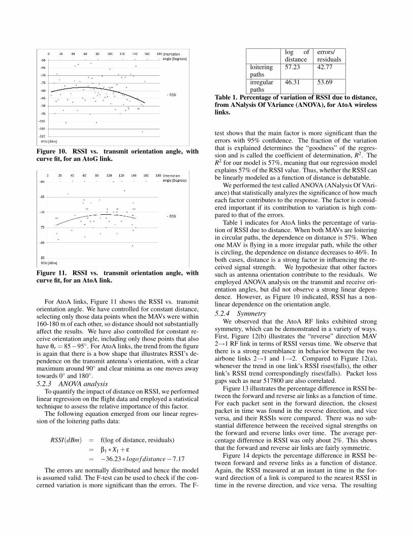
Figure 10. RSSI vs. transmit orientation angle, withcurve fit, for an AtoG link.

Figure 11. RSSI vs. transmit orientation angle, withcurve fit, for an AtoA link.

For AtoA links, Figure 11 shows the RSSI vs. transmitorientation angle. We have controlled for constant distance,selecting only those data points when the MAVs were within160-180 m of each other, so distance should not substantiallyaffect the results. We have also controlled for constant re-ceive orientation angle, including only those points that alsohave θr = 85−95◦. For AtoA links, the trend from the figureis again that there is a bow shape that illustrates RSSI’s de-pendence on the transmit antenna’s orientation, with a clearmaximum around 90◦ and clear minima as one moves awaytowards 0◦ and 180◦.5.2.3 ANOVA analysis

To quantify the impact of distance on RSSI, we performedlinear regression on the flight data and employed a statisticaltechnique to assess the relative importance of this factor.

The following equation emerged from our linear regres-sion of the loitering paths data:

RSSI(dBm) = f(log of distance, residuals)= β1 ∗X1 + ε

= −36.23∗ logo f distance−7.17

The errors are normally distributed and hence the modelis assumed valid. The F-test can be used to check if the con-cerned variation is more significant than the errors. The F-

log ofdistance

errors/residuals

loiteringpaths

57.23 42.77

irregularpaths

46.31 53.69

Table 1. Percentage of variation of RSSI due to distance,from ANalysis Of VAriance (ANOVA), for AtoA wirelesslinks.

test shows that the main factor is more significant than theerrors with 95% confidence. The fraction of the variationthat is explained determines the “goodness” of the regres-sion and is called the coefficient of determination, R2. TheR2 for our model is 57%, meaning that our regression modelexplains 57% of the RSSI value. Thus, whether the RSSI canbe linearly modeled as a function of distance is debatable.

We performed the test called ANOVA (ANalysis Of VAri-ance) that statistically analyzes the significance of how mucheach factor contributes to the response. The factor is consid-ered important if its contribution to variation is high com-pared to that of the errors.

Table 1 indicates for AtoA links the percentage of varia-tion of RSSI due to distance. When both MAVs are loiteringin circular paths, the dependence on distance is 57%. Whenone MAV is flying in a more irregular path, while the otheris circling, the dependence on distance decreases to 46%. Inboth cases, distance is a strong factor in influencing the re-ceived signal strength. We hypothesize that other factorssuch as antenna orientation contribute to the residuals. Weemployed ANOVA analysis on the transmit and receive ori-entation angles, but did not observe a strong linear depen-dence. However, as Figure 10 indicated, RSSI has a non-linear dependence on the orientation angle.5.2.4 Symmetry

We observed that the AtoA RF links exhibited strongsymmetry, which can be demonstrated in a variety of ways.First, Figure 12(b) illustrates the “reverse” direction MAV2→1 RF link in terms of RSSI versus time. We observe thatthere is a strong resemblance in behavior between the twoairbone links 2→1 and 1→2. Compared to Figure 12(a),whenever the trend in one link’s RSSI rises(falls), the otherlink’s RSSI trend correspondingly rises(falls). Packet lossgaps such as near 517800 are also correlated.

Figure 13 illustrates the percentage difference in RSSI be-tween the forward and reverse air links as a function of time.For each packet sent in the forward direction, the closestpacket in time was found in the reverse direction, and viceversa, and their RSSIs were compared. There was no sub-stantial difference between the received signal strengths onthe forward and reverse links over time. The average per-centage difference in RSSI was only about 2%. This showsthat the forward and reverse air links are fairly symmetric.

Figure 14 depicts the percentage difference in RSSI be-tween forward and reverse links as a function of distance.Again, the RSSI measured at an instant in time in the for-ward direction of a link is compared to the nearest RSSI intime in the reverse direction, and vice versa. The resulting

(a) RSSI versus time for link MAV-1-to-MAV-2

(b) RSSI versus time for link MAV-2-to-MAV-1

Figure 12. RSSI vs. time for the forward and reverselinks between two MAVs.

differences are grouped by distance. The percentage differ-ence is relatively small at all measured distances, averagingless than 2%.

5.3 Characterization of Packet LossFigure 15 shows the absolute number of packets lost as a

function of RSSI and time for one AtoG wireless link. Thex-y plane plots RSSI vs time, and shows a periodic behav-ior due to loiter circles. However, whenever a sequence ofpackets is lost, we plot the size of the sequence or gap on thez-axis, drawing a vertical line up from the last correct RSSIvalue by an amount equal to the number of consecutively lostpackets. These appear as spikes in the figure. The figure in-dicates that the frequency and height of the spikes roughlyincreases as the RSSI decreases.

To further understand where packet losses occur, we showin Figure 16 scatter plots of absolute packet loss vs. both dis-tance and RSSI for both AtoG and GtoG wireless links. ForGtoG links, Figure 16(a) shows that as distance increases,the size of packet loss gaps increases. Note that the y-axisis logarithmic. Similarly, Figure 16(b) shows that as RSSIdecreases, the size of packet loss gaps increases. The av-erage RSSI for successfully received packets was -75 dBm.As a result, the vast majority of packet losses occur belowthe average RSSI. For AtoG links, a similar though less pro-nounced pattern emerges. Figure 16(c) shows a slight trend

Figure 13. Symmetry of AtoA links: percentage differ-ence in RSSI between forward and reverse links vs. time.

Figure 14. Symmetry of AtoA links: percentage differ-ence in RSSI between forward and reverse links, as afunction of distance.

towards more severe packet losses as distance increases,while Figure 16(d) shows a slightly clearer trend towardsmore severe packet losses as RSSI drops. We believe thetrends are not as clear in these AtoG links because the planeswere relatively close to the base station during AtoG commu-nication. The average AtoG RSSI for successfully receivedpackets was -80 dBm.

Figure 17 plots the distribution of the packet loss gap sizesfor both AtoG and GtoG links. The vast majority of lossesare 1-3 packets in length. However, there are some outliergaps that are quite large, and both graphs have been truncatedfor clarity, each removing one large outlier (@163 for AtoGand @254 for GtoG).

The percentage packet loss vs. distance is shown in Fig-ure 18. Percentages were calculated by binning the distanceevery 10 m and counting the percentage of lost packets ineach bin. A gap of N packets was estimated to have occurredat an approximate distance equal to the average of the twosuccessfully received packets defining the start and end ofthe gap. An average RSSI was similarly calculated for eachgap. In this way, each gap was associated with a given dis-tance, hence a bin. The resulting percentage losses show thatour GtoG links began to lose the majority of their packets atabout a range of 250 m, while our AtoG links are much morereliable over a longer range. In particular, 20% packet loss

(a) GtoG scatter plot of packet loss gap size vs. distance. (b) GtoG scatter plot of packet loss gap size vs. RSSI.

(c) AtoG scatter plot of packet loss gap size vs. distance. (d) AtoG scatter plot of packet loss gap size vs. RSSI.

Figure 16. Scatter plots of packet loss gap sizes vs. distance and RSSI.

Figure 15. Packet loss for one circling MAV. RSSI vs.time is plotted in the x-y plane, while z-height measuresthe number of lost packets for each gap, plotted from thelast RSSI point before the loss/gap.

occurs at about 400 m for AtoG links vs. 210 m for GtoGlinks. The corresponding RSSIs at these distances, from Fig-ure 8, are about -92 dBm for AtoG links and -100 dBm forGtoG links.

We would expect AtoA links to experience even lesspacket loss than AtoG links, given the relative performancenumbers for RSSI seen in the previous subsection between

AtoG and AtoA links. However, we experienced AtoApacket loss ranging from 20-60%, rising with distance. Webelieve this was due to the way in which we were collect-ing AtoA link quality data, which relied on forwarded pack-ets in multi-hop flooding. There was only one packet bufferon each MAV in our implementation, so it is possible thateach routing MAV would lose a large fraction of forwardedpackets at each hop due to buffer overflow. The same packetloss does not occur for AtoG data because packets reach thebase station directly without being relayed by a MAV. Weare attempting to determine the source of this packet lossand improve the flooding mechanism. Because these imple-mentation effects exaggerate AtoA packet loss, and do notillustrate the impact of distance and other factors on AtoApacket loss, we have not shown the AtoA data for absolutepacket loss gap size in Figures 16 and 17. We hope to pro-vide clearer AtoA packet loss data in a journal version of thispaper.

However, Figure 18 does afford us an opportunity to plotAtoA packet loss % provided we can normalize for the effectof relay-induced packet loss. We conducted a 2-plane groundexperiment, with both planes within 1 m of each other andthe base station, to measure the amount of packet loss in-troduced by relaying. Under these circumstances, we deter-mined that baseline packet loss due to congestion/relayingaveraged about 43%. The normalized AtoA packet loss %

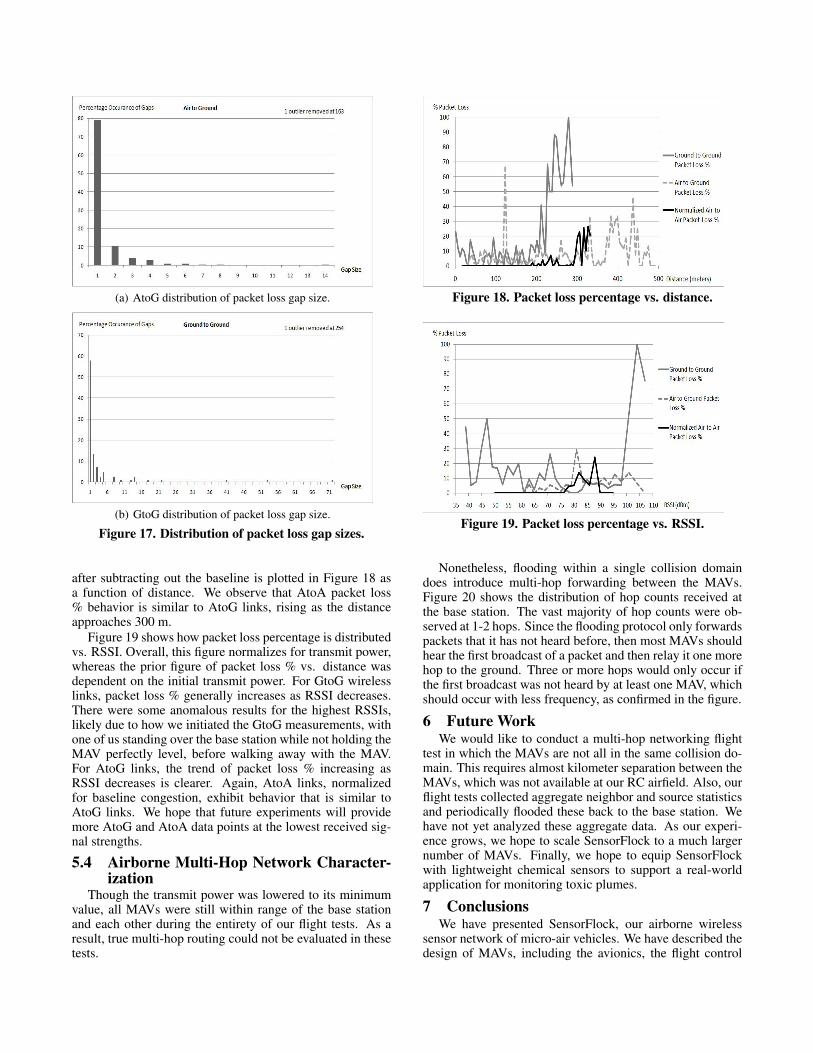
(a) AtoG distribution of packet loss gap size.

(b) GtoG distribution of packet loss gap size.

Figure 17. Distribution of packet loss gap sizes.

after subtracting out the baseline is plotted in Figure 18 asa function of distance. We observe that AtoA packet loss% behavior is similar to AtoG links, rising as the distanceapproaches 300 m.

Figure 19 shows how packet loss percentage is distributedvs. RSSI. Overall, this figure normalizes for transmit power,whereas the prior figure of packet loss % vs. distance wasdependent on the initial transmit power. For GtoG wirelesslinks, packet loss % generally increases as RSSI decreases.There were some anomalous results for the highest RSSIs,likely due to how we initiated the GtoG measurements, withone of us standing over the base station while not holding theMAV perfectly level, before walking away with the MAV.For AtoG links, the trend of packet loss % increasing asRSSI decreases is clearer. Again, AtoA links, normalizedfor baseline congestion, exhibit behavior that is similar toAtoG links. We hope that future experiments will providemore AtoG and AtoA data points at the lowest received sig-nal strengths.

5.4 Airborne Multi-Hop Network Character-ization

Though the transmit power was lowered to its minimumvalue, all MAVs were still within range of the base stationand each other during the entirety of our flight tests. As aresult, true multi-hop routing could not be evaluated in thesetests.

Figure 18. Packet loss percentage vs. distance.

Figure 19. Packet loss percentage vs. RSSI.

Nonetheless, flooding within a single collision domaindoes introduce multi-hop forwarding between the MAVs.Figure 20 shows the distribution of hop counts received atthe base station. The vast majority of hop counts were ob-served at 1-2 hops. Since the flooding protocol only forwardspackets that it has not heard before, then most MAVs shouldhear the first broadcast of a packet and then relay it one morehop to the ground. Three or more hops would only occur ifthe first broadcast was not heard by at least one MAV, whichshould occur with less frequency, as confirmed in the figure.

6 Future WorkWe would like to conduct a multi-hop networking flight

test in which the MAVs are not all in the same collision do-main. This requires almost kilometer separation between theMAVs, which was not available at our RC airfield. Also, ourflight tests collected aggregate neighbor and source statisticsand periodically flooded these back to the base station. Wehave not yet analyzed these aggregate data. As our experi-ence grows, we hope to scale SensorFlock to a much largernumber of MAVs. Finally, we hope to equip SensorFlockwith lightweight chemical sensors to support a real-worldapplication for monitoring toxic plumes.

7 ConclusionsWe have presented SensorFlock, our airborne wireless

sensor network of micro-air vehicles. We have described thedesign of MAVs, including the avionics, the flight control

Figure 20. Distribution of received hop counts at the basestation.

software, and the launch system. We have shown the capa-bility to perform controlled loiter-circle hovering of MAVs.We have provided an in-depth characterization of the RSSIbehavior for ground-to-ground, air-to-ground, and air-to-airwireless links, showing how AtoA links fall off in signalstrength with distance much less severely than GtoG links.In particular, we have quantified the path loss exponents ofGtoG (3.57), AtoG (2.13), and AtoA (1.92) wireless links.We have further conducted statistical ANOVA analysis ofRSSI dependence on distance, revealing a strong dependenceof RSSI on distance over various flight paths. Airborne linkswere shown to be roughly symmetric. The distribution ofpacket loss gap sizes showed that the vast majority of packetlosses were of size one or two packets in length. Packet losspercentage was shown to increase with increasing distanceand decreasing RSSI for AtoA, AtoG, and GtoG links, withAtoA and AtoG sharing similar behavior.

8 AcknowledgementsWe wish to thank Cory Dixon, Jack Elston, James Mack,

Michael Buettner, Carl Hartung, Wang-Ting Lin, ToddMytkowicz, and Richard Messick. We also with to thankour shepherd Thiemo Voigt and our anonymous reviewersfor their comments.

9 References[1] D. Aguayo, J. Bicket, S. Biswas, G. Judd, and R. Mor-

ris. Link-level measurements from an 802.11b meshnetwork. In SIGCOMM, August 2004.

[2] A. Akella, G. Judd, S. Seshan, and P. Steenkiste. Self-management in chaotic wireless deployments. In ACMMobiCom, 2005.

[3] B. Bellur, M. Lewis, and F. Templin. Tactical infor-mation operations for autonomous teams of unmannedaerial vehicles (UAVs). In IEEE Aerospace ConferenceProceedings, volume 6, pages 2741–2756, 2002.

[4] J. Bicket, D. Aguayo, S. Biswas, and R. Morris. Archi-tecture and evaluation of an unplanned 802.11b meshnetwork. In ACM MobiCom, 2005.

[5] T. Brown, B. Argrow, S. D. R.-G. Thekkekunnel, andD. Henkel. Ad hoc uav ground network (augnet).

In Proc. AIAA 3rd “Unmanned Unlimited” TechnicalConference, Chicago, IL, September 2004.

[6] T. Brown, S. Doshi, S. Jadhav, and J. Himmelstein. Testbed for a wireless network on small uavs. In Proc.AIAA 3rd “Unmanned Unlimited” Technical Confer-ence, Chicago, IL, September 2004.

[7] V. Bychkovsky, B. Hull, A. Miu, H. Balakrishnan, andS. Madden. A measurement study of vehicular internetaccess using in situ wi-fi networks. In ACM MobiCom,2006.

[8] K. Chebrolu, B. Raman, and S. Sen. Long-distance802.11b links: Performance measurements and experi-ence. In ACM MobiCom, 2006.

[9] Y.-C. Cheng, J. Bellardo, P. Benko, A. C. Snoeren,G. M. Voelker, and S. Savage. Jigsaw: Solving the puz-zle of enterprise 802.11 analysis. In ACM SIGCOMM,2006.

[10] ACM E-WIND (Experimental approaches towireless network design and analysis) Work-shop. http://acm.org/sigcomm/sigcomm2005/w1-e-wind.html.

[11] D. Ganesan, B. Krishnamachari, A. Woo, D. Culler,D. Estrin, and S. Wicker. Complex behavior at scale:An experimental study of low-power wireless sensornetworks. In UCLA Computer Science Technical Re-port UCLA/CSD-TR 02-0013, February 2002.

[12] M. Gerla, Y. Yi, and K. Xu. Team communicationamong airborne agents. In Proc. Of American He-licopter Society 59th Annual Forum, pages 163–167,2003.

[13] J. Grasmeyer and M. Keennon. Development of theBlack Widow micro air vehicle. AIAA paper 2001-0127, Reno, NV, 2001. 39th AIAA Aerospace SciencesMeeting & Exhibit.

[14] D. Henkel, C. Dixon, J. Elston, and T. Brown. A re-liable sensor data collection network using unmannedaircraft. In Second International Workshop on Multi-hop Ad Hoc Networks: from theory to reality (REAL-MAN), Florence, May 2006.

[15] P. Ifju, D. Jenkins, S. Ettinger, Y. Lian, W. Shyy,and M. Waszak. Flexible-wing-based micro air ve-hicles. AIAA paper 2002-0705, American Instituteof Aeronautics and Astronautics, January 2002. 40th

Aerospace Sciences Meeting & Exhibit, Reno, Nevada.

[16] E. King, M. Alighanbari, Y. Kuwata, and J. P. How. Co-ordination and control experiments on a multi-vehicletestbed. In Proceedings of the IEEE American ControlConference, pages 5315–5320, April 2004.

[17] M. Kovacina, D. Palmer, G. Yang, andR. Vaidyanathan. Multi-agent control algorithmsfor chemical cloud detection and mapping usingunmanned air vehicles. In Proc. IEEE/RSJ Conf.Intelligent Robots and Systems, pages 2782–2788,Lausanne, Switzerland, October 2002.

[18] D. Lawrence, K. Mohseni, and R. Han. Information en-ergy for sensor-reactive uav flock control. In 3rd AIAAUnmanned Unlimited Technical Conference, Workshopand Exhibit, September 2004. AIAA paper 2004-6530.

[19] G. Lu, B. Krishnamachari, and C. Raghavendra. Per-formance evaluation of the ieee 802.15.4 mac for low-rate low-power wireless networks. In Workshop onEnergy-Efficient Wireless Communications and Net-works (EWCN ’04), held in conjunction with the IEEEInternational Performance Computing and Communi-cations Conference (IPCCC), April 2004.

[20] K. Pahlavan and A. Levesque. Wireless InformationNetworks. John Wiley & Sons, 1995.

[21] M. Petrova, J. Riihijarvi, P. Mahonen, and S. Labella.Performance study of ieee 802.15.4 using measure-ments and simulations. In Proceedings of IEEE WCNC,April 2006.

[22] W. J. Pisano and D. A. Lawrence. Autonomousuav control using a 3-sensor autopilot. In AIAA In-foTech@Aerospace Conf., Sonoma, CA, May, 2007.

[23] T. Rappaport. Wireless Communications: Principlesand Practice. Prentice Hall, 2002.

[24] A. Woo and D. Culler. Taming the challenges of re-liable multihop routing in sensor networks. In ACMSenSys, November 2003.

[25] K. Xu, X. Hong, and M. Gerla. Landmark routing inad hoc networks with mobile backbones. Journal ofParallel and Distributed Computing (JPDC), SpecialIssues on Ad Hoc Networks, 2002.

[26] K. Xu, X. Hong, M. Gerla, H. Ly, and D. Gu. Land-mark routing in large wireless battlefield networks us-ing UAVs. In IEEE MILCOM, pages 230–234, 2001.

[27] Y. J. Zhao and R. Govindan. Understanding packet de-livery performance in dense wireless sensor networks.In ACM SenSys, 2003.

[28] J. Zheng and M. J. Lee. A comprehensive perfor-mance study of IEEE 802.15.4. IEEE Press, Wiley In-terscience, 2006.

[29] G. Zhou, T. He, S. Krishnamurthy, and J. Stankovic.Impact of radio irregularity on wireless sensor net-works. In ACM Mobisys, June 2004.