SENSOR TEAM #3 - The CentMesh...
21
Transcript of SENSOR TEAM #3 - The CentMesh...

1. Project Goal: The overall goal of the project was to design and build a drone, capable of flying in an
indoor environment without crashing. Specifically, this drone will be piloted and have a control and sensor system capable of deterring it from hitting obstacles. It will also have a camera to record images with enough quality to be used for piloting, and will have to sustain the temperatures and wind speeds of a harsh environment such as that of a building fire.
1.1 Module Goal: We were one of the teams tasked with building the sensor module. The goal of the
sensor module is to detect obstacles in the drone’s vicinity, accurately and promptly. Preferably, the module should have detection in 360 degrees in three dimensions and should be able to accurately detect obstacles, and report the data to the control module. The project will begin with the selection of the sensors, follow with characterization and modelling of the individual sensors, and then fusion of one modality of sensor data, the distances given by the ultrasonic sensors, and another modality, the acceleration given from the IMU.The fused data will then be sent to the control module in the form of 6 safe distances, each pointing in a different orthogonal direction from the drone. All of this must be done while minimizing cost and weight, but without reducing accuracy to the point of unacceptable performance degradation.

2. Sensor Module Design
2.1 Sensor selection: Lidar: Lidar was initially an option to consider due to its accuracy and longer range. Lidar is
used in Neato Robotic Vacuums to detect obstacles. Lidar however does detect smoke as an obstacle which would present issues for a drone operating in environments where smoke is very prevalent. Also these Lidar units were still too expensive to be seriously considered for this project.
Short Range Radar: Short range radar is also very effective at sensing object from a distance and unlike
lidar units, short range radar is not affected by smoke. However short range radar units are costly, and multiple sensors would be needed to complete the goal. For these reasons it would not complete the goal within a reasonable budget.
Ultrasonic Sensors: Ultrasonic sensors are very cheap, replaceable and simple sensors to interpret.
However the range of ultrasonic sensors is very limited as well as its beam width. For that reason many sensors would be needed to successfully complete the goal. Another issue with ultrasonic sensors is potential interference with other sensors. Ultrasonic sensor’s readings also vary with the temperature in the room which can cause poorer readings. Nevertheless, due to the cost constraints, and given the price of the other options, ultrasonic sensors are the only viable option to complete the goal within a reasonable budget.
SRF02 Ultrasonic Rangefinder: The best ultrasonic sensor to accomplish the goal of the sensor module is the SRF02
Ultrasonic Range Finder. With a beamwidth of 60 degrees 14 sensors can create a full 360 degree coverage as outlined in our goals. It has a maximum range of 6 meters however that range changes as objects become smaller and the angle become steeper. Figure 2.1 below displays the SRF02’s maximum detection range of a 55mm diameter plastic pipe.

Figure 2.1 SRF02 Detection Cone
The SRF02 has a minimum detection range of 17 cm. The SRF02 is also small measuring at 24 x 20 x 17 mm and only weighs 4.6 grams. At that weight, all 14 sensors required for the sensor module, weigh only 64.4 grams which is well within the weight constraint provided by the airframe. Each sensors transmits sound at 40kHz and draws typically 20 mW of power. The sensors can be connected to a microcontroller via serial or I2C. Each sensor can be given an address from 0 to 15 allowing 16 sensors to be connected to one port. SRF02 is connected to the microcontroller as displayed below in Figure 2.2
Figure 2.2 SRF02 Circuit Layout
9 Degrees of Freedom Razor IMU: This IMU uses a threeaxis gyroscope, a threeaxis accelerometer, and a threeaxis
magnetometer. Through a serial connection it is possible to get the orientation and acceleration of the drone. The thought behind using an IMU is to attempt to leverage two different modalities of sensor data, ultrasonic distances to obstacles, and acceleration of the drone. In order to construct a fused estimated of obstacle distances and drone position. By fusing these two different kinds of sensor data, we eliminate a lot of the gaussian noise associated with all sensor measurements, and additionally filter out most of the erroneous data. This is commonly referred to as Data Fusion, and is a common technique in signal processing.

2.2 Algorithm Considerations or “Why we chose to use an IMU”:
In our case, the idea was to take the acceleration measurements from the IMU, remove the portion that corresponds to gravity (leaving us with just the acceleration of the drone), and integrate that acceleration. Once to get velocity, twice to get position. We could also get an estimate of position from the ultrasonic sensor data, by tracking the change in distance to obstacles over time.
Both these techniques would allow us to keep track of the position the drone was in, relative to its starting position. We would then fuse these two estimates of position. And use the resulting, more accurate, position estimate to not only get a better estimate of obstacle distance, but also to map the environment.
We ended up deciding to use a state estimator. Initially we tried a Kalman Filter, which is in itself a type of state estimator, but is perhaps too complex of a tool for our purposes and is more obscure and therefore more difficult to tune to make work correctly. The state estimator essentially keeps track of previous states ( in our case position, velocity and acceleration) and predicts the next states based on the recent history(trend) of said states. It then computes an error term that is the difference between the predicted states and the measured states, and based on that error term, it picks a compromise between the predicted state based on past measurements, and the measured state, to be the current state.
SLAM stands for simultaneous location and mapping. Given that using the above
techniques we can get both an estimate of position and of distances to nearest obstacles, this allows us to incrementally construct a map of the explored environment. This will aid in the exploration of the building, speeding up backtracking and keeping track of what locations have been passed by already, and it could also be incorporated into the collision detection. If accurate enough SLAM could mean that backtracking through a previously explored environment is swift and predictable.
2.3 Microcontroller Selection:
The BeagleBone Black microcontroller was chosen due to it versatility, effectiveness to
accomplish the goals, as well as it availability. As a class, it was decided that the BeagleBone Black would be an effective microcontroller for any group and if everyone used it, the combination of modules would be easier in the future. For the sensor module it provided everything we needed. As seen in the pin layout below, the BeagleBone Black has plenty of GPIO ports that can be configured for use as well as 4 UART ports that have been preconfigured for serial communication. The BeagleBone Black also has a linux operating system and 2 Gigabytes of memory. This amount of processing and storage power will be helpful when creating the SLAM mapping

Figure 2.3 BeagleBone Black Pinout
2.4 Sensor Layout and Frame:
In order to get 360 degrees of coverage, using a sensor beam width of 60 degrees, the
following layout was designed. 12 sensors are equally spaced around the drone. Six sensors would be mounted at a 30 degree angle up and the other six more sensors are mounted at a 30 degree angle down. One sensor is mounted vertically up and one more is mounted vertically down. This layout is visually demonstrated below in Figure 2.4.

TOP: SIDE:
Figure 2.4 SRF02 Cone Layout In order to accomplish this layout we constructed a model in Solidworks and 3D
printed it to create the frame in Figure 2.5. The frame allows for easy mounting of 14 sensors as designed and allows for 360 degrees of coverage.
Figure 2.5 Mount Design 1

3. Building Process 3.1 Sensor Layout: Due to delays and time constraints, the layout of the sensors was simplified to a 5 sensor
configuration, to be used as a proof of concept. Even though we don’t have the 14 sensors required to get full 360 degree coverage, a proof of concept can still be completed with a reduced number of sensors and an IMU. With 5 sensors enough data can be obtained to fuse with the IMU to prove that the tracking system and obstacle avoidance works, and will be even more effective in the 14 sensor system.
3.2 Frame Redesign: In order to test the 5 sensors proof of concept, a new frame had to be designed. The
frame shown in Figure 3.1 is the new frame. It allows for 5 sensors to be mounted at once. It also provides space for the IMU, breadboard and microcontroller.
Figure 3.1 Mount Design 2
3.3 Sensor Setup: Each sensor needed proper wiring in order to connect to the microcontroller. Using 1x5
pins, 2x5 prototype board and 12 cm wire strands, each sensor was connected using basic soldering techniques. After that, each sensor was given a number 04. This number corresponds to the address assigned to the sensor so that the BeagleBone Black can

properly communicate with it. At this point the sensors should look something similar to Figure 3.2.
Figure 3.2 Wired SRF02 Sensors
Each sensor’s address is initially 0x00 and thus 4 of the sensors have to be changed. In
order to do this, connect the individual sensor to the BeagleBone as shown in Figure 3.3. Rx will be connected to P9_22 of the BeagleBone Black and Tx will be connected to P9_21. Mode will be connected to ground for serial mode.
Figure 3.3 SRF02 Circuit Layout
Once the sensor is properly connected to the microcontroller, send the change of
address message. In order to communicate with the sensor, each message is prefaced with the current address assigned to the sensor. In this case the current address is 0x00. The change of address message is 0xA0, 0xAA, 0xA5, 0x0_. The final byte will determine the new address for the sensor. These commands must follow the correct sequence and no other command may be sent in the middle of the sequence. The sequence must be sent as four separate commands to the address 0x00. For example to change the address to 0x05 the following sequence will do that. 0x00, 0xA0 then 0x00, 0xAA, then 0x00, 0xA5 and finally 0x00, 0x05. after changing the address ranging can begin. To initiate a ranging in centimeters send the command 84 or 0x54. Either one of the three commands initiants ranging as well as transmits the result of the ranging back to the BeagleBone Black when available. A further breakdown of all commands in below in Table 3.1.

Command Action
Decimal Hex
81 0x51 Real Ranging Mode Result in centimeters
84 0x54 Real Ranging Mode Result in centimeters, automatically Tx range back to controller as soon as ranging is complete.
95 0x5F Get Minimum, returns two bytes (high byte first) of the closest range measurable see Autotune section
96 0x60 Force Autotune Restart same as powerup. You can ignore this command.
Table 3.1 SRF02 Commands After each sensor has been given an address, all the sensors can be connected to the
BeagleBone together. With 4 UART ports total and one for the IMU, 3 are left for the sensors to be connected to. Connect 2 sensors, in this case sensor 1 and 3, to UART 2. The Tx of the sensors will be connected to P9_22 of the BeagleBone Black, and the Rx will be connected to P9_21. Connect 2 more sensors, in this case 2 and 4, to UART 4. The Tx of these sensors will be connected to P9_11 of the BeagleBone Black, and the Rx will be connected to P9_13. Finally connect the last sensor (sensor 0) to UART 5 by connecting the Tx to P8_38 and the Rx to P8_37 of the BeagleBone. Be sure to connect each sensor to VCC and ground. Attach the sensors and BeagleBone Black to the frame using velcro stickers and the sensor module will look like Figure 3.3

Figure 3.4 Sensor Module
3.4 Estimating Position using the SRF02 Sensors: In order to run SLAM, it was necessary to get position based on the change in
distance reported by the SRF02 sensors. This was accomplished by measuring the change in distance of sensors facing opposite directions. If only one of the sensors reported a change in the distance then the least amount of change was used. This was done to prevent incorrect position estimating, in cases where the distance change wasn’t due to the motion of the drone, but instead due to an object entering the drone’s field of view. This case is shown below in Figure 3.4. As seen, an object appears on one side of the drone. The distance on the left of the drone decreased due to the object, however, the drone remained on its current path. This is known because the right side sensors did not report a change in distance. Thus, the position estimate is computing using the distance from the sensor in the right.
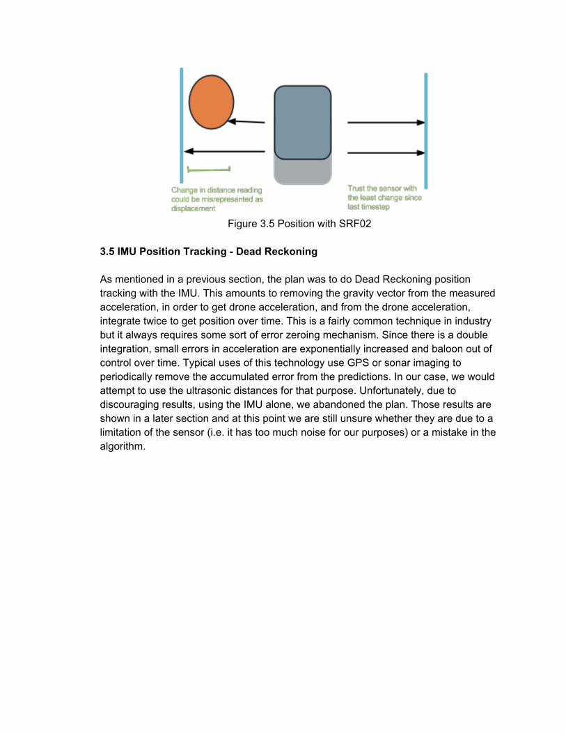
Figure 3.5 Position with SRF02
3.5 IMU Position Tracking Dead Reckoning As mentioned in a previous section, the plan was to do Dead Reckoning position tracking with the IMU. This amounts to removing the gravity vector from the measured acceleration, in order to get drone acceleration, and from the drone acceleration, integrate twice to get position over time. This is a fairly common technique in industry but it always requires some sort of error zeroing mechanism. Since there is a double integration, small errors in acceleration are exponentially increased and baloon out of control over time. Typical uses of this technology use GPS or sonar imaging to periodically remove the accumulated error from the predictions. In our case, we would attempt to use the ultrasonic distances for that purpose. Unfortunately, due to discouraging results, using the IMU alone, we abandoned the plan. Those results are shown in a later section and at this point we are still unsure whether they are due to a limitation of the sensor (i.e. it has too much noise for our purposes) or a mistake in the algorithm.

3.6 IMU Orientation Tracking
In order to effectively perform SLAM, the orientation of the drone must either remain constant or be incorporated into the mapping. The IMU’s magnetometer outputs an yaw, Θ, which can directly be applied to SLAM. Figure 3.6 shows how with the yaw and some simple trigonometry, the point can be accurately plotted.
Figure 3.6 IMU Orientation
Plot Point = [ Position Y + Distance*cos(Θ), Position X + Distance*sin(Θ) ]
3.7 SLAM
SLAM is created by taking the position data created by the sensors and IMU and plotting the distance readings from the position points. When done correctly the result is a visual map of the space around the drone. For example, if traveling down a hallway with doors, one would expect the SLAM results to be two very straight lines with breaks at the doorways as shown in Figure 3.7.
Figure 3.7 SLAM Tracking

4.0 Testing and Proof of Concept Results: 4.1 Accuracy of SRF02: The first thing tested after setting up the sensors was the precision of the SRF02
Sensors. We found quickly that in an indoor environment that our SRF02 data was very reliable from within 3 meters and greater than 15 cm.
4.2 Accuracy of IMU: For the IMU however we found that the data we received for acceleration was
accurate but not normalized for gravity. Thus while remaining still, the acceleration readings in the Z axis were 9.8 m/s. In order to use the IMU acceleration data this gravity had to be removed. Using the acceleration and magnetometer data one can compute the orientation vector of the drone. That orientation vector can then be multiplied by the gravity vector [0,0,9.81] and subtracted from the measured acceleration to end up with the relative acceleration. Unfortunately slight errors in the orientation vector due to noise in the sensors can cause large errors in the estimated relative acceleration. With data fusion these errors should theoretically be able to be diminished or removed, but under the scope of this project, we couldn’t get it to work.
4.3 Refresh Rates of Sensors:
The accuracy and reliability of the SRF02 sensor was very good however the refresh
rate on our module was only about 7hz. This is because the SFR02 requires 60ms of wait time in order for the sound to return from a 9m distance away, which is the sensor’s max range. Due to this physical limitation, and due to propagation and calculation times within the circuit, the SFR02 datasheet suggests a 70ms wait time between subsequent measurements. It was also necessary to stack two sensors on one UART port because the BeagleBone Black only had 4 preconfigured UART ports. If each sensor was connected to a single port the refresh rate would double to 14 or 15hz. For testing purposes, 7hz was acceptable however if used by the drone each sensor should have its own UART configured port.

4.4 Sensor Distance, Position, SLAM Results: Hallway Test Trial 1: In the Hallway Test, it was possible to test the performance of the SRF02 ultrasonic
sensors, the positioning algorithm, as well as the SLAM capabilities. In order to interpret the results more easily, a consistent environment with only one or two changing elements was prefered. Thus a hallway with an open door was chosen. In trial one, the module was moved at a constant speed down the hallway and past an open door. Figure 5.1 displays the SLAM map (top), position along the hallway (middle), and the sensor readings facing the wall with the open door (bottom). The sensor data was very reliable and consistent while traveling along the wall and accurately detects the wall through the door. However in this first trial, the position jumps several meters suddenly and then remains constant which is not what happened. This causes the SLAM map to expand the doorway and clump points together around 750 cm. It is not know why this occurred but it did not happen again in later trials.
Figure 5.1 Hallway Trial 1
Hallway Test Trial 2: In Trial 2 the door is clearly visible around 50 as the distance estimation in this case
was much smoother. Once again the distance measurements were extremely reliable and consistent when facing a wall.

Figure 5.2 Hallway Trial 2

4.5 IMU Acceleration, Velocity, Position Results: Trial 1: Trial 1 consisted of moving in the positive X direction then back to the starting point.
Followed by positive Y motion and back to the start. Lastly positive Z motion and back to the start. Figures 5.3, 5.4, and 5.5 display the acceleration in the X,Y, and Z planes respectively.
Figure 5.3 IMU Trial 1 X Axis
Figure 5.4 IMU Trial 1 Y Axis

Figure 5.5 IMU Trial 1 Z Axis
Following Trial 1 there was promise that the IMU position tracking could be implemented in an effective manner as the positions of X,Y, and Z moved in accordance to the actual motion. However even though in trial 1 the motion was captured, the distances were not accurate. The module was moved 20cm in each direction but the peak of the X axis was at 30cm, the Y axis peaked at 40cm and the Z axis peaked at 1 meter. Unfortunately, this error is too great for this data to be used as an accurate means of measuring position.
Trial 2: Trial 2 was only moving the module 20cm in the positive X direction, however the results,
this time, did not even accurately replicate the motion. The X position went to 20 cm and began to return to 0 but then went to 40 cm which does not reflect the motion. There was also no significant motion in the Y or Z axis but our results have significant motion in those directions. After numerous result like these it seemed apparent that the IMU’s acceleration was too unreliable to accurately track position to the degree of accuracy needed for reliable position estimation.

Figure 5.6 Trial 2 X Axis
Figure 5.7 Trial 2 Y Axis
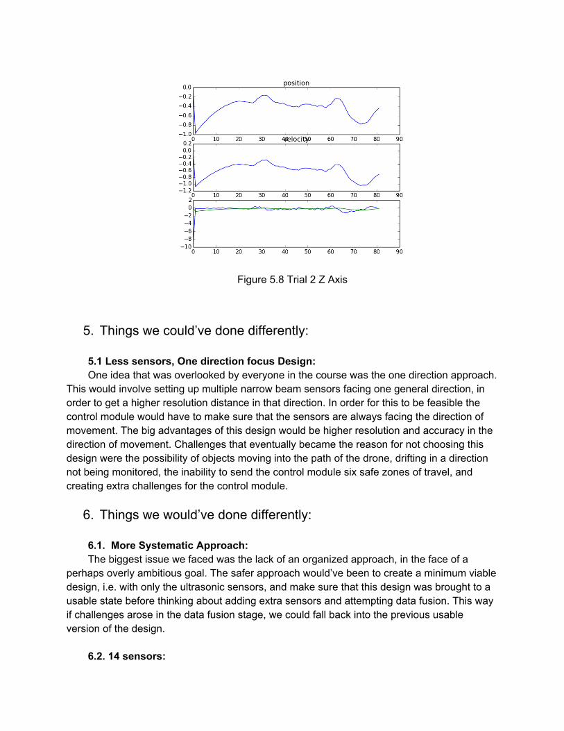
Figure 5.8 Trial 2 Z Axis
5. Things we could’ve done differently: 5.1 Less sensors, One direction focus Design: One idea that was overlooked by everyone in the course was the one direction approach.
This would involve setting up multiple narrow beam sensors facing one general direction, in order to get a higher resolution distance in that direction. In order for this to be feasible the control module would have to make sure that the sensors are always facing the direction of movement. The big advantages of this design would be higher resolution and accuracy in the direction of movement. Challenges that eventually became the reason for not choosing this design were the possibility of objects moving into the path of the drone, drifting in a direction not being monitored, the inability to send the control module six safe zones of travel, and creating extra challenges for the control module.
6. Things we would’ve done differently: 6.1. More Systematic Approach: The biggest issue we faced was the lack of an organized approach, in the face of a
perhaps overly ambitious goal. The safer approach would’ve been to create a minimum viable design, i.e. with only the ultrasonic sensors, and make sure that this design was brought to a usable state before thinking about adding extra sensors and attempting data fusion. This way if challenges arose in the data fusion stage, we could fall back into the previous usable version of the design.
6.2. 14 sensors:

The most obvious thing to improve upon is testing the module with 14 sensors instead of 5. This would give a 360 degree view of obstacles without any blind spots and would still work and interface with the IMU. However, with 14 sensors we would most likely also have more interference issues and therefore more noisy data. Solutions could be, physical shielding of the sensors to glancing sound waves, or better filtering algorithms.
6.3. More Accessible frame to avoid chaotic wiring: One issue that arose during the construction of the module was how chaotic the wiring
became. Wiring needed to be thought of and incorporated into the design of the frame. Also color coded wires would help with the organization and getting rid of the breadboard for a more permanent wiring setup would also help
6.4. Configure GPIO pins as UARTs to improve ultrasonic sensor refresh rate: Configuring the GPIO pins in the BeagleBone Black as UARTs would require some
coding. But this would allow for each sensor to be connected to its own port, as opposed to the current setup, where two sensors share a port, effectively halving their refresh rate. Giving each sensor its own port would double our refresh rate, from 7Hz to about 15Hz and allow for more data, more accurate detection of obstacles, and better position tracking with the aid of the IMU.