Sensor Selection for Relative Acoustic Transfer Function ...

1220 IEEE/ACM TRANSACTIONS ON AUDIO, SPEECH, AND LANGUAGE PROCESSING, VOL. 29, 2021

Sensor Selection for Relative Acoustic TransferFunction Steered Linearly-Constrained Beamformers

Jie Zhang , Member, IEEE, Jun Du , Senior Member, IEEE, and Li-Rong Dai

Abstract—For multi-microphone speech enhancement, differ-ent microphones might have different contributions, assome areeven marginal. This is more likely to happen in wireless acousticsensor networks (WASNs), where somesensors might be distant.In this work, we therefore consider sensor selection for linearly-constrained beamformers. Theproposed sensor selection approachis formulated by minimizing the total output noise power andconstraining thenumber of selected sensors. As the consideredsensor selection problem requires the relative acoustic transferfunction(RTF), the covariance whitening based RTF estimation ora direct-path RTF approximation is exploited. For a singletargetsource, we can thus substitute the estimated RTF or the assumedRTF to the original problem formulation in orderto design aminimum variance distortionless response (MVDR) beamformer.Alternatively, we can integrate the two RTFsto design a linearlyconstrained minimum variance (LCMV) beamformer in order toalleviate the effects of RTFestimation/approximation errors. Byleveraging the superiority of LCMV beamformers, the proposedapproach can beapplied to the multi-source case. An evaluationusing a simulated large-scale WASN demonstrates that the integra-tion ofRTFs for the sensor selection based LCMV beamformer canbe beneficial as opposed to relying on either of theindividual RTFsteered sensor selection based MVDR beamformers. We concludethat the sensors that are close to thetarget source(s) and also somearound the coherent interferers are more informative.

Index Terms—Beamformers, convex optimization, covariancewhitening, relative acoustic transfer function, sensor selection,speech enhancement, wireless acoustic sensor networks.

I. INTRODUCTION

M ICROPHONE arrays are frequently deployed in vari-ous audio applications, e.g., hearing aids (HAs) [1],

teleconferencing systems [2], hands-free telephony [3], speechrecognition [4], human-robot interaction [5], etc. Although thetraditional array system has been widely studied over the pastfew decades, its configuration brings several limitations, leadingto a bottleneck with respect to the speech processing perfor-mance. Usually, conventional array systems are equipped with

Manuscript received October 13, 2020; revised January 26, 2021; acceptedMarch 3, 2021. Date of publication March 8, 2021; date of current versionMarch 26, 2021. This work was supported in part by the Fundamental ResearchFunds for the Central Universities under Grant WK2100000016, in part by theNational Key R&D Program of China under Grant 2017YFB1002202, and in partby the Leading Plan of CAS under Grant XDC08010200. The associate editorcoordinating the review of this manuscript and approving it for publication wasM. M. Doss. (Corresponding author: Jie Zhang.)

The authors are with the National Engineering Laboratory for Speechand Language Information Processing, University of Science and Technol-ogy of China (USTC), Hefei 230026, China (e-mail: [email protected];[email protected]; [email protected]).

Digital Object Identifier 10.1109/TASLP.2021.3064399

multiple microphones, which are physically linked to a centralcomputing unit. Rearranging such a wired and centralized arraysystem (e.g., including a new microphone or removing a uselessmicrophone) seems impractical. The spatial sampling capabilityis limited, as the location of the microphone arrays cannot bechanged easily. In case the microphones are distant from thetarget speaker, low-quality audio recordings are obtained andthe system performance degrades. Moreover, the size of thearrays should be determined by the application scenarios, forexample, only a small array consisting of 2-4 microphones canbe equipped by each HA.

Nowadays, with the increased popularity of using wireless de-vices, e.g., laptops, smartphones, we are surrounded by wirelessacoustic sensor networks (WASNs). In WASNs, each node canbe mounted with a single microphone or a small microphone ar-ray. Due to the capability of wireless communication, the sensornetwork can be organized more flexibly, either in a centralizedfashion or in a distributed way [6]–[9]. The utilization of WASNsfor speech processing can potentially resolve the limitationswithin the conventional microphone array systems. For instance,as the wireless devices can be distributed anywhere, they mightbe very close to the target source, resulting in high-qualityrecordings which are beneficial for speech enhancement. Eventhough the HAs can only host a rather limited number of micro-phones, if the external wireless devices share their measurementswith the HAs, they are able to make use of more data, leading toa performance improvement [10]–[12]. However, incorporatingmore external sensors as a WASN in return requires a higherpower consumption and computational complexity. In this con-text, the challenges need to be addressed are 1) how to optimallyselect the most informative subset of sensors from a large-scaleWASN? and 2) how to reconstruct the target speech signal fromthe incomplete observations over the WASN?

The concept of sensor selection originates from wirelesssensor networks (WSNs) [13]. Mathematically, it can be for-mulated by optimizing a certain performance measure subjectto a constraint on the cardinality of the selected subset, or in theother way around. In principle, sensor selection is a combina-torial optimization problem. In order to perform sensor selec-tion efficiently, some convex relaxation techniques [13]–[15] orgreedy heuristics (e.g., submodularity) [16] should be leveraged.Using the selected subset of sensors can still perform sourcelocalization [14], field estimation [17], target tracking [15], etc,yet the resource consumption is saved, as much less sensorsare involved. In WASNs, there are also some sensor selectionalgorithms that have been proposed recently for e.g., speech

2329-9290 © 2021 IEEE. Personal use is permitted, but republication/redistribution requires IEEE permission.See https://www.ieee.org/publications/rights/index.html for more information.

Authorized licensed use limited to: University of Science & Technology of China. Downloaded on August 01,2021 at 14:38:11 UTC from IEEE Xplore. Restrictions apply.

https://orcid.org/0000-0003-1124-0854

https://orcid.org/0000-0002-2387-0389

mailto:[email protected]



ZHANG et al.: SENSOR SELECTION FOR RELATIVE ACOUSTIC TRANSFER FUNCTION STEERED LINEARLY-CONSTRAINED BEAMFORMERS 1221

enhancement [18]–[20], speech recognition [21], and speakertracking [22]. It was shown in [20] that sensor selection iseffective in reducing the power consumption and computationalcomplexity for WASNs with a tolerable scarification of noisereduction performance.

A. Contributions

In this work, we consider to select the most informative subsetof sensors from a large-scale WASN for linearly constrainedbeamformers based speech enhancement, such that the targetspeech signal can be estimated using a subset of microphoneobservations. The considered sensor selection problem is formu-lated by minimizing the total output noise power and constrain-ing the number of selected sensors. Since the audio recordingsacross different microphones are highly correlated, using allmeasurements from the complete network is unnecessary and alarge amount of resource consumption is required. By using theproposed sensor selection algorithm, the data redundancy canthus be removed to some extent and the resource consumptioncan be saved.

We begin with the sensor selection in the context of mini-mum variance distortionless response (MVDR) beamforming(SS-MVDR) for a single source estimation. As the originalSS-MVDR optimization problem requires the relative acoustictransfer function (RTF), we consider two variants: 1) using anestimated RTF and 2) exploiting an assumed RTF, as the RTFcan be approximated using a priori information. As there existestimation errors in the estimated RTF and approximation errorsin the assumed RTF, using the respective RTF would affect theoptimality of sensor selection and further degrade the speech en-hancement performance. Then, we integrate the two constraintsassociated with the estimated and assumed RTFs to design alinearly constrained minimum variance (LCMV) beamformerand consider the sensor selection criterion for such an LCMVbeamformer (SS-LCMV). Both SS-MVDR and SS-LCMV canbe derived as semi-definite programming problems using convexoptimization techniques.

Further, we analyze that for the single target source case theobtained SS-LCMV can be approximated as an integration oftwo SS-MVDRs, but SS-LCMV is more robust against the RTFestimation/approximation errors. The selected subset obtainedby SS-LCMV can be viewed as the intersection set between theselected subsets obtained by the two SS-MVDR methods. In casethe estimated (or assumed) RTF is more reliable, the selectedsubset of SS-LCMV will be more similar to that by the estimated(or assumed) RTF steered SS-MVDR. Therefore, compared toSS-MVDR, the proposed SS-LCMV method is able to automat-ically check the reliability of involved RTFs. Due to the fact thatthe LCMV beamformer can handle multiple sources, we furtherapply the proposed SS-LCMV algorithm to a multi-source case,where the RTFs are estimated sequentially. Experimental resultsusing a simulated WASN validate the proposed approaches. Wefind that the sensors close to the existing sources are more likelyto be selected, as the sensors around the target source(s) arehelpful for enhancing the target signal(s) and those close to theinterfering source(s) (even having a low signal-to-noise ratio)

are beneficial for suppressing the noise signal(s). Using theintegrated RTFs can refine the selected subset of sensors andimprove the noise reduction performance.

In [20], we proposed a microphone subset selection methodfor MVDR (MSS-MVDR) beamformer based noise reduction,which is formulated by minimizing the total power consumptionover the WASN and constraining the desired noise reductionperformance. In principle, MSS-MVDR is a special case of theproposed SS-MVDR problem, as the total power consumptionis directly linked to the cardinality of the selected subset. On theother hand, MSS-MVDR was solved based on the assumptionthat the acoustic transfer function (ATF) of a single source isgiven. The ATF estimation error would affect the selection ofMSS-MVDR significantly. Therefore, the proposed SS-MVDRcan be seen as a generalization of MSS-MVDR, and the pro-posed SS-LCMV is an extension of MSS-MVDR, which is morepractical and applicable to a more dynamic scenario. Comparedto the utility-based sensor selection method that was proposedin [18], [23], the proposed method can achieve a better noisereduction performance in case the number of the selected sensorsis fixed.

B. Outline and Notations

The rest of this paper is structured as follows. Section IIintroduces the required preliminary knowledge, including signalmodel, the covariance whitening based RTF estimation methodand linearly-constrained beamformers (e.g., MVDR, LCMV).Section III presents the proposed sensor selection method in thecontext of MVDR beamforming. In Section IV, we extend theproposed method to a more general LCMV framework with asingle source and multiple sources being taken into account.Section V presents the experimental results using a simulatedWASN. Finally, Section VI concludes this work.

The notation used in this paper is as follows: Upper (lower)bold face letters are used for matrices (column vectors). (·)T or(·)H denotes (vector/matrix) transposition or conjugate trans-position. E(·) denotes the mathematical expectation operation.diag(·) refers to a block diagonal matrix with the elements in itsargument on the main diagonal. 1N and ON denote the N × 1vector of ones and the N ×N matrix with all its elements equalto zero, respectively. IN is an identity matrix of size N . A � Bmeans that A−B is a positive semidefinite matrix. |U| denotesthe cardinality of the set U .

II. FUNDAMENTALS

A. Signal Model

In this work, we consider a WASN consisting of M spatiallydistributed acoustic sensor nodes, which are exploited for sam-pling and monitoring the acoustic scene of interest. Without lossof generality, we assume that each node is composed of a singlemicrophone. Letting l and ω, respectively, denote the frameindex and the frequency index, in the short-time Fourier trans-form (STFT) domain, the recorded signal at the kth microphone,say Yk(ω, l), can be written as

Yk(ω, l) = Xk(ω, l) +Nk(ω, l), k = 1, . . . ,M, (1)



where Xk(ω, l) denotes the target signal component at micro-phone k, and Nk(ω, l) the noise component recorded by the kthmicrophone, which can incorporate coherent noise sources (e.g.,competing speakers) and incoherent noises (e.g., late reverber-ation of the target source, sensor thermal noise).

For the single point source case, which is characterized by theATF ak(ω) (relating the target source position to microphone k),the signal component is then given by

Xk(ω, l) = ak(ω)S(ω, l), (2)

whereS(ω, l) denotes the target signal. Note that (2) holds underthe assumption that the target source keeps static, implying thatthe ATF of this source is time-invariant. Without loss of gener-ality, taking the first microphone as the reference microphone,which can be chosen using a more sophisticated method in [24],and defining the RTF as

hk(ω) = ak(ω)/a1(ω), (3)

then the signal component equals

Xk(ω, l) = hk(ω)X1(ω, l), (4)

whereX1(ω, l) = a1(ω)S(ω, l). The introduction of RTF is dueto the fact that in practice RTF can be estimated using covariancesubtraction or covariance whitening method [25]–[27], howeverdirectly estimating ATF is still unknown. More importantly, theutilization of RTF does not degrade the beamforming perfor-mance. For notational conciseness, we will omit the frame andfrequency indexes in the sequel bearing in mind that all thefollowing operations are realized in the STFT domain. Let thevector y stack the microphone measurements for each time-frequency bin, i.e., y = [Y1, Y2, . . . , YM ]T . Similarly, we definethe vectors x, n, a and h for stacking the signal components,noise components, the ATF and the RTF, respectively, such thatthe considered signal model can also be given by

y = hX1 + n. (5)

Furthermore, we assume that the target source and the noisecomponents are mutually uncorrelated, such that the relationshipbetween the second-order statistics can be formulated as

Φyy = E{yyH

}= E

{xxH

}+ E

{nnH

}= Φxx +Φnn, (6)

where Φxx and Φnn denote the correlation matrix of the signalcomponents and the correlation matrix of the noise components,respectively. For a single target source case, Φxx is a rank-1matrix in theory, since by definition we have

Φxx � σ2Saa

H � σ2X1

hhH , (7)

where σ2S = E{|S|2} and σ2

X1= E{|X1|2} denote the power

spectral density (PSD) of the target source and the PSD of thesignal component at the reference microphone, respectively. Inpractice, these correlation matrices can be estimated using theaverage smoothing technique. For instance, given a perfect voiceactivity detector (VAD), the microphone signal can be classifiedinto speech-absent frames and speech-plus-noise frames. Duringthe two periods, the noise and noisy correlation matrices can beestimated, respectively.

The key procedure of the linearly constrained beamformingtechnique is to design a linear filter w = [w1, w2, . . . , wM ]T ,

such that the estimated target signal at the chosen referencemicrophone can be obtained through beamforming as

X1 = wHy. (8)

B. Covariance Whitening Based RTF Estimation (CW-RTF)

For the design of such a beamformer, the RTF estimate isrequired. Among various RTF estimation approaches, it wasshown in [27] that the eigen-decomposition based covariancewhitening method has a superiority in performance, particularlyin noisy and strong reverberant environments. However, it ismore complex compared to, e.g., covariance subtraction, fromthe perspective of implementation, since the time consumingmatrix inversion or matrix decomposition is involved. In thiswork, in order to alleviate the impact of RTF estimation onsensor selection based noise reduction, we adopt the covariancewhitening method to estimate the RTF vector.

Given the microphone measurements y per time-frequencybin and the estimated noise correlation matrix Φnn, the covari-

ance whitening method uses Φ−1/2

nn to whiten y as

y = Φ−1/2

nn y, (9)

where Φ1/2

nn is the square root of Φnn. Then, the correlationmatrix of the whitened signals can be calculated using theaverage smoothing technique as

Φyy =1

Ly

Ly∑l=1

y(l)y(l)H (10)

� Φ−1/2

nn ΦyyΦ−H/2

nn , (11)

where Ly denotes the number of speech-plus-noise segments.Note that Φyy and Φyy should be estimated using the sameframe set. Let φ denote the principal eigenvector of Φyy, i.e.,

Φyyφ = λmaxφ, (12)

where λmax is the maximum eigenvalue of Φyy. With φ, thecovariance whitening based RTF estimate is given by

hCW =Φ

1/2

nn φ

eH1 Φ1/2

nn φ, (13)

where e1 is a column vector with the first entry equal to one andzeros elsewhere. Notably, it is easy to check that the covariancewhitening based RTF estimate is equivalent to the normalizedprincipal eigenvector of the generalized eigenvalue decomposi-tion (GEVD) of the matrix pencil {Φyy, Φnn}.

C. MVDR Beamformer

The well-known MVDR beamformer is formulated by mini-mizing the output noise power under a linear constraint, whichis exploited for preserving the signal power that comes fromthe direction of interest. Mathematically, it can be designed byconsidering the following constrained optimization problem:

wMVDR = argminw

wHΦnnw s.t. wHh = 1. (14)

With such a linear constraint and using (7), we can see thatwH

MVDRΦxxwMVDR = σ2X1

, which implies that the power of



the desired signal component at the reference microphone ispreserved. Any reduction of the objective function is caused byreducing the noise power. Given the true RTF vectorh and usingthe technique of Lagrangian multipliers, the MVDR beamformercan be shown to be given by [28], [29]

wMVDR = (hHΦ−1

nnh)−1Φ

−1

nnh. (15)

The output noise power of MVDR beamformer is given by

wHMVDRΦnnwMVDR = (hHΦ

−1

nnh)−1, (16)

and the output signal-to-noise ratio (SNR) is given by

oSNRMVDR = σ2X1

hHΦ−1

nnh. (17)

Obviously, the optimal design of the MVDR beamformer isdependent on the true RTF, which is unknown, the optimalMVDR beamformer is thus impractical to approach. In practice,we can substitute a priori information on RTF into (14) to obtainnear-optimal, but more practical solutions.

1) MVDR Based on the Estimated RTF (MVDR-EST): Onealternative way to design a practical MVDR beamformer isbased on the use of the estimated RTF vector. Substituttingthe RTF estimate from (13) into (15), the resulting MVDRbeamformer is then given by

wMVDR−EST = (hHCWΦ

−1

nnhCW)−1Φ−1

nnhCW. (18)

2) MVDR Based on an Assumed RTF (MVDR-ASS): In somecases, the RTF of the target source can be approximated by usinga priori assumptions. For example, for the hearing-aid users,usually the target source is located in the front direction. In thiscontext, the RTF of the target source can be approaximated bygain and delay values as

hASS =[1, g21e

−j2πfτ21 , . . . , gM1e−j2πfτM1

], (19)

where gk1 is the attenuation coefficient which depends on thedistance between the source position and the microphone pair,and τk1, ∀k denotes the time-difference of arrival (TDOA).Therefore, one can use the assumed RTF hASS for a practi-cal MVDR implementation. The resulting near-optimal MVDRbeamformer is then given by

wMVDR−ASS = (hHASSΦ

−1

nnhASS)−1Φ

−1

nnhASS. (20)

Note that under the utilization of an estimated RTF or an as-sumed counterpart, the signal power cannot be exactly preservedany more as using the true RTF, because there exist estima-tion/approximation errors.

D. LCMV Beamformer

An important limitation within the classic MVDR beam-formers is that the distortionless response corresponding to onedirection (which is characterized by the estimated RTF hCW

or the assumed RTF hASS) can be preserved. Clearly, in casethe mismatch between the involved RTF and the true RTF islarge, the performance of the MVDR beamformer will degradesignificantly. For this, one can add more linear constraints tothe MVDR optimization problems. These linear constraints areassociated with multiple directions, such that the distortionlessresponse from more RTFs can be preserved, resulting in an

LCMV beamformer as

wLCMV = argminw

wHΦnnw s.t. CHw = b, (21)

where the matrix C ∈ CM×N is constructed from multipleRTFs, and the vector b ∈ CN is dedicated to enforcing thedistortion level for each RTF. Similarly, the LCMV beamformercan be resolved as a close-form solution:

wLCMV = Φ−1

nnC(CHΦ−1

nnC)−1b. (22)

The output noise power of LCMV filter is then given by

wHLCMVΦnnwLCMV = bH(CHΦ

−1

nnC)−1b. (23)

Remark 1: In order to further visualize the LCMV beam-former, one can consider a special case. Given

C = [hCW, hASS], b = [1, 1]T , (24)

the resulting LCMV beamformer is a linear combination of thetwo MVDR beamformers based on the use of the estimated andassumed RTFs [30], i.e.,

wLCMV = α1wMVDR−EST + α2wMVDR−ASS, (25)

where α1 and α2 depends on the estimated and assumedRTFs and the noise correlation matrix, and are detailed in [30,Sec. III-C]. Clearly, the LCMV beamformer is a generalizationof the MVDR filter. Since the LCMV beamformer takes moreconstraints into account, less degrees of freedom are left foradjusting the filter coefficients to minimize the noise power.

III. SENSOR SELECTION FOR MVDR BEAMFORMING

In this section, we will present the proposed SS-MVDRmethod for speech enhancement using a subset of microphonemeasurements over a large-scale WASN.

A. Sensor Selection Model

The sensor selection problem is formulated by choosing abest subset of sensors in order to optimize an objective functionsubject to certain constraints. For this, we first introduce aBoolean selection vector

p = [p1, p2, . . . , pM ]T ∈ {0, 1}M ,

where pk = 1, ∀k indicates that the kth microphone is selected,and otherwise unselected. Further, we use K = ||p||0 to rep-resent the number of selected sensors with �0-norm denotingthe number of non-zero elements of a vector. Letting diag(p)denote a diagonal matrix whose diagonal entries are given byp, we can define a selection matrix Σp ∈ {0, 1}K×M which isobtained by removing the all-zero rows of diag(p). Clearly, wecan obtain the following properties:

ΣpΣTp = IK , ΣT

pΣp = diag(p). (26)

With the selection matrix at hand, we can construct the incom-plete audio measurements as

yp = Σpy = Σpx+Σpn ∈ CK . (27)

Similarly, the RTF and noise correlation matrix associated withthe selection sensors are given by

hp = Σph ∈ CK , Φnn,p = ΣpΦnnΣTp ∈ CK×K . (28)



The MVDR beamformer depending on the selected sensors isthen given by

wp =(hHp Φ

−1

nn,php

)−1

Φ−1

nn,php, (29)

where we note that in general Φ−1

nn,p �= ΣpΦ−1

nnΣTp , unless Φnn

is diagonal (i.e., the uncorrelated noise case). As a result, theestimated target signal can be obtained as X1 = wH

p yp.

B. Problem Formulation (SS-MVDR)

Given the RTF (e.g., hCW, hASS), the proposed sensor selec-tion for MVDR beamforming can be formulated by minimizingthe total output noise power under a constraint that the signal as-sociated with the considered RTF is undistorted, as the followingconstrained optimization problem shows

minp,wp

wHp Φnn,pwp

s.t. wHp hp = 1

||p||0 ≤ K, p ∈ {0, 1}M ,

(30)

where K denotes the maximum number of sensors that can beselected, which can be assigned by users. Obviously, this is anon-convex optimization problem, because of the non-linearselection operation by selection matrix Σp and the Booleanvariables p. However, we can simplify it for analysis. Consid-ering the Lagrangian function of (30) and calculating the partialderivative with respect to wp, we find that the MVDR beam-former is the solution. Hence, plugging the MVDR beamformerfrom (29) into (30), we obtain a simplified sensor selectionproblem:

maxp

hHp Φ

−1

nn,php

s.t. ||p||0 ≤ K, p ∈ {0, 1}M ,

(31)

By doing this, we can get rid of jointly optimizing the originalproblem over two variables. The simplified version only needsto consider the selection variable, which indeed is still a non-convex (combinatorial) optimization problem.

C. Convex Solver

In this section, we will resolve the proposed sensor selectionproblem following convex optimization techniques and usingthe true RTF h. Note that the proposed solver also applies tothe case of using the estimated RTF hCW or the assumed RTFhASS. First of all, in order to avoid the non-linearity within

hHp Φ

−1

nn,php, we consider to decompose the matrix Φnn as

Φnn = λI+G, (32)

where the constant λ is positive and G is a positive semi-definitematrix. Since Φnn is always positive definite in the presenceof correlated and uncorrelated noises, we can find such a de-composition via eigenvalue decomposition (EVD) of Φnn. Forexample, λ can be chosen to be the minimum eigenvalue of Φnn.Even though λ might be close to zero, as long as λ > 0, (38) willbe always feasible. With λ and G at hand, it can be seen that

Φnn,p = ΣpΦnnΣTp = λIK +ΣpGΣT

p . (33)

Further, the objective function of (31) can be derived as

hHp Φ

−1

nn,php = hH ΣTp

(λIK +ΣpGΣT

p

)−1Σp︸︷︷︸

Q

h. (34)

Using the matrix inversion lemma [31]

C(B−1 +CTA−1C)−1CT = A−A(A+CBCT )−1A,

the matrix Q can be represented as

Q = G−1 −G−1(G−1 + λ−1diag(p)

)−1G−1. (35)

With Q, we can equivalently re-write (31) in an epigraph formas [32]

maxp,η

η

s.t. η ≤ hHQh

||p||0 ≤ K, p ∈ {0, 1}M ,

(36)

Substituting Q from (35) into the constraint η ≤ hHQh, weobtain

hHG−1h− η ≥ hHG−1(G−1 + λ−1diag(p)

)−1G−1h,

which can be reformulated as a symmetric linear matrix inequal-ity (LMI) [32] using the Schur complement[

G−1 + λ−1diag(p) G−1h

hHG−1 hHG−1h− η

]� OM+1, (37)

due to the fact that the matrix G−1 + λ−1diag(p) is alwayspositive definite with a positive λ and a positive semi-definitematrix G−1.

Now the non-convexity of (31) lies in the �0-norm and theBoolean constraint. For the �0-norm, one alternative is by usingthe �1-norm which is convex to relax it. For the Boolean con-straint, it can be relaxed using continuous surrogates or semi-definite relaxation [33]. In this work, we will relax pk ∈ {0, 1}to 0 ≤ pk ≤ 1, ∀k. To this end, we can represent the originalSS-MVDR problem as

maxp,η

η

s.t.

[G−1 + λ−1diag(p) G−1h

hHG−1 hHG−1h− η

]� OM+1

1TMp ≤ K, 0 ≤ pk ≤ 1, ∀k, (38)

which is a semi-definite programming problem and can be effi-ciently solved in polynomial time using interior-point methodsor some off-the-shelf solvers, like CVX [34] or SeDuMi [35].The computational complexity of (38) is cubic in terms ofM . The final Boolean solution can be obtained by randomizedrounding or deterministic rounding techniques. Note that (38) isa general sensor selection problem for the RTF-steered MVDRbeamformer. In practice, given the noise statistics, we can sub-stitute the estimated RTF hCW or the assumed RTF hASS into(38) to solve a specific, but more practical problem.



IV. SENSOR SELECTION FOR LCMV BEAMFORMING

Since using the estimated RTF hCW or the assumed RTF hASS

might distort the target signal, similar to SS-MVDR we thus pro-pose a sensor selection based LCMV (SS-LCMV) beamformerin this section.

A. General Sensor Selection for LCMV (SS-LCMV)

The considered sensor selection based LCMV beamformer isformulated by minimizing the total output noise power under aset of linear constraints together with the cardinality constraint,as the following optimization problem shows

minp,wp

wHp Φnn,pwp

s.t. CHp wp = b

||p||0 ≤ K, p ∈ {0, 1}M ,

(39)

where Cp = ΣpC ∈ CK×N . Again, (39) is a non-convex com-binatorial optimization problem. In order to find an efficientsolver for (39), similarly to Section III, we consider its Lagrangefunction and derive the partial derivative with respect towp. Theresulting beamformer wp is then given by

wp = Φ−1

nn,pCp

(CH

p Φ−1

nn,pCp

)−1

b, (40)

which is the classic LCMV beamformer given in (22), but nowdepends on the selected subset of sensors. Under the utilizationof such an LCMV beamformer, the output noise power in theobjective function of (39) is given by

wHp Φnn,pwp = bH

(CH

p Φ−1

nn,pCp

)−1

b. (41)

Substituting (41) into (39), we can therefore get rid of opti-mizing the filter coefficients, and only the selection variable isunknown. The original problem can then be simplified as

minp

bH(CH

p Φ−1

nn,pCp

)−1

b

s.t. ||p||0 ≤ K, p ∈ {0, 1}M .

(42)

By introducing a new variable η, (42) can be equivalentlyreformulated in the following epigraph form:

minp,η

η

s.t. bH(CH

p Φ−1

nn,pCp

)−1

b ≤ η

||p||0 ≤ K, p ∈ {0, 1}M .

(43)

In order to linearize the first constraint in (43), we introduce asymmetric positive semi-definite matrix T ∈ SN

+ , such that itcan be relaxed as two new constraints:

bHT−1b ≤ η, (44)

CHp Φ

−1

nn,pCp � T. (45)

Clearly, (44) and (45) are sufficient to obtain the first constraintin (43). Furthermore, using the Schur complement (44) can bereformulated as an LMI[

T b

bH η

]� ON+1. (46)

The left-hand side of (45) can be shown to be given by

CHp Φ

−1

nn,pCp = CHQC, (47)

where Q is given by (see Section III-C)

Q = G−1 −G−1(G−1 + λ−1diag(p)

)−1G−1.

Hence, (45) can be re-written as

CHG−1C−T � CHG−1(G−1 + λ−1diag(p)

)−1G−1C,

(48)which can further be reformulated as an LMI:[

G−1 + λ−1diag(p) G−1C

CHG−1 CHG−1C−T

]� OM+N . (49)

In addition, we relax the cardinality constraint �0-norm in(43) using the corresponding �1-norm, and relax the Booleanconstraint using the box counterpart, such that (43) can bereformulated in a semi-definite programming form as

minp,η,T

η

s.t.

[T b

bH η

]� ON+1

[G−1 + λ−1diag(p) G−1C

CHG−1 CHG−1C−T

]� OM+N

1TMp ≤ K, 0 ≤ pk ≤ 1, ∀k, (50)

which can be efficiently solved by exploiting convex optimiza-tion techniques as before. Note that the computational com-plexity of solving (50) is of the order of O((M +N)3). Thefinal Boolean selection variables should be recovered by usingrounding techniques.

B. Relation to SS-MVDR

For the single target source case, either applying the estimatedRTF hCW or using the assumed RTF hASS to the SS-MVDRoptimization problem in Section III might not achieve the bestsubset of sensors, leading to a decrease in the noise reductionperformance, due to the errors between the involved RTFs andthe true one. In this case, using both RTFs and consideringthe sensor selection for LCMV beamforming, we can obtainan instantiation of (50). Let

Cp = [hCW,p, hASS,p] = [ΣphCW,ΣphASS], b = [1, 1]T ,

The corresponding LCMV beamformer can be computed as

wp = α1w1,p + α2w2,p, (51)

where the weights α1 and α2 can be calculated [30], and therespective MVDR beamformers are given by

w1,p =Φ

−1

nn,phCW,p

hHCW,pΦ

−1

nn,phCW,p

, w2,p =Φ

−1

nn,phASS,p

hHASS,pΦ

−1

nn,phASS,p

.

Applying such an LCMV beamformer, the resulting total outputnoise power can be calculated as

wHp Φnn,pwp=

|α1|2hHCW,pΦ

−1

nn,phCW,p

+|α2|2

hHASS,pΦ

−1

nn,phASS,p



Fig. 1. The residual noise power (in dB) in terms of the number of the selectedsensor using different RTFs.

+2R⎛⎝ α∗

1α2hHCW,pΦ

−1

nn,phASS,p

hHCW,pΦ

−1

nn,phCW,phHASS,pΦ

−1

nn,phASS,p

⎞⎠ ,

(52)

where the operation R(·) extracts the real part of a complexnumber, and the first (or second) term represents the residualnoise power using the estimated (or assumed) RTF steeredMVDR beamformer. The third term denotes the residual noisepower using the mixed RTF. In order to analyze the functionof each term, we consider the experimental setup as shownin Fig. 2(a) and randomly select K sensors to perform beam-forming. The estimated RTF is obtained using the covariancewhitening method, and the assumed RTF is calculated using (19),so the assumed RTF is much more accurate than the estimatedone. In Fig. 1, we show the residual noise power in terms ofthe number of selected sensors using different RTFs. It is clearthat in case the assumed RTF is more accurate, the noise powerobtained by using the mixed RTF approaches that obtained usingthe estimated RTF. In case the estimated RTF is more accurate,the noise power can be compared similarly. Therefore, we canapproximate wH

p Φnn,pwp using

wHp Φnn,pwp≈ (1 + μ1)|α1|2

hHCW,pΦ

−1

nn,phCW,p

+(1 + μ2)|α2|2

hHASS,pΦ

−1

nn,phASS,p

,

(53)where μ1 and μ2 denote the confidence level of hCW andhASS, respectively, and μ1 + μ2 = 1. In case the assumed RTFis more accurate, μ1 > μ2; otherwise μ2 > μ1. Note that theintroduction of this approximation is to find the link between theproposed SS-MVDR and SS-LCMV methods. A more accuratederivation for (52) is left to the reader. Substituting (51) and(53) into the general LCMV problem description in (39), wearrive at

minp

(1 + μ1)|α1|2hHCW,pΦ

−1

nn,phCW,p

+(1 + μ2)|α2|2

hHASS,pΦ

−1

nn,phASS,p

s.t. ||p||0 ≤ K, p ∈ {0, 1}M ,

(54)

which can further be re-written in an epigraph form as

minp,η1,η2

(1 + μ1)|α1|2η1

+(1 + μ2)|α2|2

η2

s.t. hHCW,pΦ

−1

nn,phCW,p ≥ η1

hHASS,pΦ

−1

nn,phASS,p ≥ η2

||p||0 ≤ K, p ∈ {0, 1}M .

(55)

Based on the decomposition of the matrix Φnn and the intro-duction of the matrix Q, the two inequality constraints in (55)can be reformulated as two LMIs (similar to (37)). Following theconvex relaxation strategies in Section III-C, (55) can be relaxedas a semi-definite programming problem:

minp,η1,η2

(1 + μ1)|α1|2η1

+(1 + μ2)|α2|2

η2

s.t.

[G−1 + λ−1diag(p) G−1hCW

hHCWG−1 hH

CWG−1hCW − η1

]� O

[G−1 + λ−1diag(p) G−1hASS

hHASSG

−1 hHASSG

−1hASS − η2

]� O

1TMp ≤ K, 0 ≤ pk ≤ 1, ∀k. (56)

Remark 2: By inspection, (56) can be regarded as an inte-gration of two sensor selection problems, which are designedusing the estimated RTF hCW and the assumed RTF hASS basedMVDR beamformers, respectively. Let the estimated RTF hCW

based MVDR sensor selection problem refer to as SS-MVDR-EST, and the selected subset of sensors from (38) be denoted bySEST. Let the assumed RTF hASS based MVDR sensor selectionproblem refer to as SS-MVDR-ASS, and the correspondingselected subset be denoted by SASS. Further, we refer to (56)which is based on the integration of two RTFs as SS-LCMV-INT,and the selected subset of sensors as SINT. From the perspectiveof sensor selection, SINT should be the intersection betweenSEST and SASS. In order to more clearly see the link between(56) and (38), we can consider two extreme cases. In case |α1|2is too small, the second term in the objective function of (56)dominates, then SS-LCMV-INT reduces to SS-MVDR-ASS.This means that the assumed RTF approximates the true RTFwell and the estimated one is not trustable. In case |α2|2 → 0,the first term dominates, then SS-LCMV-INT reduces to SS-MVDR-EST. This means that the covariance whitening methodprovides a good RTF estimate.

C. Application to the Multi-Source Case

In the presence of multiple target speech sources, which arerequired to be preserved at the output of a linearly constrainedbeamformer, we need to design an LCMV beamformer, as theMVDR filter can only handle a single source. We assume thatthere areN ≥ 2 sources, and let hi, ∀i denote the estimated RTFof the ith source with respect to the sensor nodes. Then, we cansubstitute

C = [h1, h2, . . . , hN ], b = 1N , (57)



Fig. 2. Sensor selection examples where the blue sensors are activated by different approaches for K = 40: (a) SS-MVDR-EST, (b) SS-MVDR-ASS, (c)SS-LCMV-INT, (d) SS-utility-EST, which uses the estimated RTF for sensor selection (the selection result of SS-utility-ASS is similar).

into (50) to obtain the most informative subset of sensors. Werefer to this multi-source case as SS-LCMV-N.

From the implementation view of point, the RTF estimation ofmultiple sources can be estimated using, e.g., [36]. To improvethe accuracy, we will estimate the RTF of each source suc-cessively in this work. Specifically, given the noise correlationmatrix Φnn which is estimated during the training phase anda perfect VAD, we can detect the speech-plus-noise segments,in which only one speech source of interest is active and theother target sources are inactive. During this period, the noisycorrelation matrix can be estimated via average smoothing (e.g.,Eq. (10)). Using the covariance whitening method, the RTFof this active source can thus be estimated. The RTF of othersources is estimated similarly. Note that for the multiple sourcecase, the number of candidate sensors should be larger than thenumber of sources, i.e., M > N , such that there are M −Ndegrees of freedom left for adjusting the beamformer coefficientsto perform noise reduction.

To this end, we have shown the sensor selection for RTF-steered MVDR and LCMV beamformers. It was shown thatusing the estimated RTF and the assumed RTF for LCMV isan integration of two individual SS-MVDR solutions. Also,the proposed general LCMV sensor selection algorithm canbe extended to the multiple source case. We summarize theproposed algorithms in Table I.

TABLE IA SUMMARY OF SENSOR SELECTION FOR RTF-STEERED LINEARLY

CONSTRAINED BEAMFORMERS

V. EXPERIMENTS

In this section, we will validate the proposed approaches vianumerical simulations. At first, we will present the experimen-tal setup and the comparison approaches. Then the proposedmethods will be applied to the single target source case. Finally,we will consider the application of the proposed SS-LCMV-Nmethod to the multi-source scenario.

Experimental setup: Fig. 2 shows the typical experimentalsetting that we use in the simulations. We consider a 2D roomwith dimensions (12× 12) m, where 169 candidate microphonesare uniformly distributed. All the speech sources are originatedfrom the TIMIT database [37], and all the noise signals from theNoiseX-92 database [38]. The room impulse responses (RIRs)of directional sources are generated using the toolbox [39]. Themeasurements of each microphone are synthesized by summing:



1) the source component (convolving the source signal and itsRIR), 2) interference component (convolving the interferer (i.e.,a competing speaker) and the corresponding RIR) and 3) theuncorrelated sensor noise (i.e., microphone self noise). The un-correlated noise is modeled as a white Gaussian noise. The signalto interferer ratio (SIR) and the signal to uncorrelated noise ratio(SNR) are set to be 0 dB and 50 dB, respectively. The finalsignal-to-interferer-noise ratio (SINR) is around -2 dB. All thesignals are sampled at 16 kHz. The signals are segmented usinga square-root-Hann window with a length of 32 ms and 50%overlap. The reverberation time is set to be T60 = 200 ms. Inorder to focus on the sensor selection problem, the microphonesignals are synchronized already in this work, and the noisecorrelation matrix is estimated during 15 seconds speech-absentperiod before performing the online sensor selection algorithms(e.g., using the average smoothing technique or [40]). The noisesource positions are assumed to be static.

Comparison methods: In [18], [23], a utility-based sensorselection approach was proposed. Since in principle sensorselection is a combinatorial optimization problem, the utility-based method greedily removes the sensor that has the leastcontribution to the noise reduction task from the total sensor set(i.e., backward selection), or adds the sensor that has the largestcontribution to the selected subset (i.e., forward selection). Ob-viously, the utility-based method can only determine the statusof one sensor at each iteration. The procedure works like asub-modularity based optimization problem [41]. Since usuallythe cardinality of the selected subset is rather smaller than thetotal number of sensors, in order to save the number of iterations,we will adopt the forward selection strategy for comparison.As the utility-based method also requires the RTFs, we willdesign two variants. In case the covariance whitening based RTFestimate is used, the utility-based method will be referred to asSS-utility-EST; in case the assumed RTF is exploited, it is thenreferred to as SS-utility-ASS.

Further, a random selection method will be compared to theproposed method, which randomly selectsK sensors to performbeamforming. Using the estimated or assumed RTF, we thusobtain two variants of the random procedure, which are referredto as random-EST and random-ASS, respectively. Note thatthe performance of the random selection methods is averagedover 100 trails. In addition, as usually a microphone signal isdominated by the target/interfering source in case the sourceis close to the microphone, it is somehow reasonable that themicrophones close to the source(s) are more informative fornoise reduction. Therefore, we will also compare a maxEnergymethod, which selects K sensors that have the largest inputpower. Similarly, using the estimated or assumed RTF, we canobtain maxEnergy-EST or maxEnergy-ASS.

A. Simulations for a Single Target Source

In this part, we consider the proposed sensor selection forthe single target source case. The target point speech source(red dot) is located at (3.6, 8.4) m. We also place a coherentinterfering source (blue star) at (8.4, 3.6) m. The variance ofthe signals is controlled by the SIR parameter. We use the

Fig. 3. Beam patterns (in dB) in terms of 2D spatial positions with K = 40.

RTF model in (19) for free fields as the assumed RTF, whichis obtained by exploiting the source position in combinationwith the microphone positions. In reverberant environments, thismodeling indeed reveals the direct-path component of the sourcesignal. Further, we set μ1 = 0.95 and μ2 = 0.05.

Fig. 2 illustrates some typical sensor selection examplesobtained by different approaches for K = 40. Clearly, for allcomparison methods, most of the selected sensors are close tothe target source, as these microphones can record high-qualitysignals, leading to a great contribution to speech enhancement.Comparing SS-MVDR-EST or SS-utility-EST to SS-MVDR-ASS, due to the RTF estimation errors, the obtained selectedsubset of sensors might not be optimal, as some sensors that arefar away from the sources are also selected. Since the assumedRTF that is exploited by SS-MVDR-ASS is based on the exactuse of source position and sensor positions, it can improve theselection performance, as the selected sensors are more assem-bled around the source position. Comparing SS-LCMV-INT toSS-MVDR-EST, it is clear that the selected subset is refinedby integrating the superiority of SS-MVDR-ASS. From theperspective of set theory, the selected subset of SS-LCMV-INTcan thus be viewed as the intersection set between the two subsetsobtained by SS-MVDR-EST and SS-MVDR-ASS. The corre-sponding beam patterns for the angular frequency ω = 0.02πrad are shown in Fig. 3, from which we can observe that themainlobes of SS-LCMV-INT are more concentrated to the truesource position.

Fig. 4 shows the output noise power (in dB) of the comparisonmethods in terms of the cardinality of the selected subset for T60

= 200 ms. Comparing SS-MVDR-ASS (or SS-utility-ASS) toSS-MVDR-EST (or SS-utility-EST), it is clear that the use ofthe assumed RTF can improve the noise reduction performancein moderately reverberant situations, since the assumed RTFrepresents the accurate direct-path propagation of the targetsource. More importantly, the proposed SS-LCMV-INT methodachieves the minimum output noise power, i.e., the best speechestimation quality. This reveals that integrating the estimatedRTF and the assumed RTF is beneficial for sensor selectionbased linearly-constrained beamformers. Due to the fact thatthe proposed methods are based on a global optimization strat-egy, the proposed SS-MVDR-EST (or SS-MVDR-ASS) methodperforms better than SS-utility-EST (or SS-utility-ASS) which



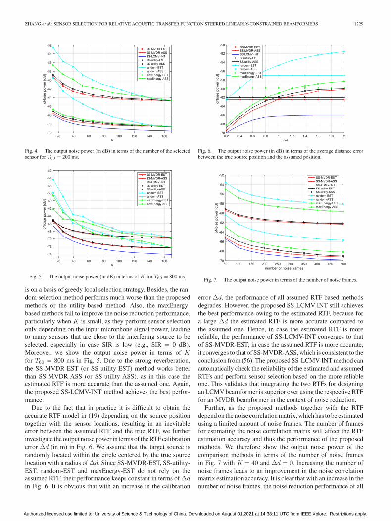
Fig. 4. The output noise power (in dB) in terms of the number of the selectedsensor for T60 = 200 ms.

Fig. 5. The output noise power (in dB) in terms of K for T60 = 800 ms.

is on a basis of greedy local selection strategy. Besides, the ran-dom selection method performs much worse than the proposedmethods or the utility-based method. Also, the maxEnergy-based methods fail to improve the noise reduction performance,particularly when K is small, as they perform sensor selectiononly depending on the input microphone signal power, leadingto many sensors that are close to the interfering source to beselected, especially in case SIR is low (e.g., SIR = 0 dB).Moreover, we show the output noise power in terms of Kfor T60 = 800 ms in Fig. 5. Due to the strong reverberation,the SS-MVDR-EST (or SS-utility-EST) method works betterthan SS-MVDR-ASS (or SS-utility-ASS), as in this case theestimated RTF is more accurate than the assumed one. Again,the proposed SS-LCMV-INT method achieves the best perfor-mance.

Due to the fact that in practice it is difficult to obtain theaccurate RTF model in (19) depending on the source positiontogether with the sensor locations, resulting in an inevitableerror between the assumed RTF and the true RTF, we furtherinvestigate the output noise power in terms of the RTF calibrationerror Δd (in m) in Fig. 6. We assume that the target source israndomly located within the circle centered by the true sourcelocation with a radius of Δd. Since SS-MVDR-EST, SS-utility-EST, random-EST and maxEnergy-EST do not rely on theassumed RTF, their performance keeps constant in terms of Δdin Fig. 6. It is obvious that with an increase in the calibration

Fig. 6. The output noise power (in dB) in terms of the average distance errorbetween the true source position and the assumed position.

Fig. 7. The output noise power in terms of the number of noise frames.

error Δd, the performance of all assumed RTF based methodsdegrades. However, the proposed SS-LCMV-INT still achievesthe best performance owing to the estimated RTF, because fora large Δd the estimated RTF is more accurate compared tothe assumed one. Hence, in case the estimated RTF is morereliable, the performance of SS-LCMV-INT converges to thatof SS-MVDR-EST; in case the assumed RTF is more accurate,it converges to that of SS-MVDR-ASS, which is consistent to theconclusion from (56). The proposed SS-LCMV-INT method canautomatically check the reliability of the estimated and assumedRTFs and perform sensor selection based on the more reliableone. This validates that integrating the two RTFs for designingan LCMV beamformer is superior over using the respective RTFfor an MVDR beamformer in the context of noise reduction.

Further, as the proposed methods together with the RTFdepend on the noise correlation matrix, which has to be estimatedusing a limited amount of noise frames. The number of framesfor estimating the noise correlation matrix will affect the RTFestimation accuracy and thus the performance of the proposedmethods. We therefore show the output noise power of thecomparison methods in terms of the number of noise framesin Fig. 7 with K = 40 and Δd = 0. Increasing the number ofnoise frames leads to an improvement in the noise correlationmatrix estimation accuracy. It is clear that with an increase in thenumber of noise frames, the noise reduction performance of all



Fig. 8. Sensor selection examples where the blue sensors are activated by different approaches for K = 60: (a) SS-MVDR-EST, (b) SS-MVDR-ASS, (c)SS-LCMV-INT, (d) SS-utility-EST, which uses the estimated RTF for sensor selection. The considered scenario includes two target sources (red solid dots) andtwo coherent interfering sources (blue stars).

approaches improves, and the proposed SS-LCMV-INT methodachieves the best performance.

B. Application to the Multiple Source Case

In this section, we apply the proposed SS-LCMV-N method tothe scenario with multiple target sources. The experimental setupis shown in Fig. 8. Two target point sources are placed at (2.4,9.6) m and (9.6, 9.6) m, respectively. Two coherent interferingsources are located at (2.4, 2.4) m and (9.6, 2.4) m, respectively.The other required parameters are set similarly as before. Notethat the RTFs of the two target sources are estimated using thecovariance whitening method one by one. Given a perfect VADand the noise statistics, we detect the segments where the firsttarget source is active and the other target is inactive, and duringthis period the corresponding RTF is estimated. This procedureapplies to the RTF estimation of the other target source. Again,the assumed RTFs of the target sources are approximated by thedirect-path RTF model in (19) based on the source positions incombination with the microphone locations. For the comparisonapproaches, in case the estimated RTFs are applied to (56), theproposed SS-LCMV-N is referred to as SS-LCMV-EST. If theassumed RTF is used in (56), it is then called SS-LCMV-ASS.Similarly to the integration of the estimated RTF and the as-sumed RTF in the single source case, we can also integrate theestimated RTFs and assumed RTFs of the two target sources as

a spanned LCMV beamformer, referred to as SS-LCMV-INT(which includes four linear equality constraints in this case).

Fig. 8 illustrates typical sensor selection examples obtainedby SS-LCMV-EST, SS-LCMV-ASS, SS-LCMV-INT and SS-utility-EST, respectively. Obviously, the proposed methodsachieve a superiority over the utility-based method, as theregions of the sources are detected. The proposed methodscan effectively select some sensors that are close to the targetsources (having a high SNR) and some that are also close to theinterfering sources (having a low SNR), which are beneficialfor enhancing the targets and suppressing the noise sources,respectively. The selection results of SS-LCMV-EST and SS-LCMV-ASS only differ in a very limited number of sensors, andthe intersection of them results in the selection of the proposedSS-LCMV-INT approach.

VI. CONCLUSION

In this paper, we investigated the selection of a subset ofsensors from a large amount of candidate sensors for the linearlyconstrained beamformers based speech enhancement issue. Theproposed sensor selection problem was formulated by minimiz-ing the total output noise power and constraining the cardinalityof the selected subset, as the number of selected sensors directlyaffects the system complexity. In the context of both MVDR andLCMV, the considered sensor selection problem can be solved



using convex optimization techniques. The proposed method isapplicable to both the single target source case and the multiplesource case. It was shown that the sensors that close to the targetsource(s) and some close to the interfering source(s) are morelikely to be selected.

Given the estimated/assumed RTF of a single source, we canuse the proposed SS-MVDR-EST/SS-MVDR-ASS method tofind the subset of informative sensors. By integrating the esti-mated RTF and the assumed RTF from the MVDR beamformersto design an LCMV beamformer, the proposed SS-LCMV-INTmethod is obtained. It was shown that the integration of RTFs canimproves the noise reduction performance, as SS-LCMV-INTcan perform sensor selection based on the reliability of therespective RTFs. As the LCMV beamformer based on the twoconstraints associated with the estimated and assumed RTFscan be regarded as a linear combination of the two MVDRbeamformers, the selected subset by SS-LCMV-INT indeed isthe intersection between the two subsets obtained by SS-MVDR-EST and SS-MVDR-ASS. In case the estimated RTFs is morereliable, the selected subset of sensors by SS-LCMV-INT ismore dominated by the sensors selected by SS-MVDR-EST;otherwise the sensors selected by SS-MVDR-ASS will domi-nate. Therefore, the proposed SS-LCMV-INT method is morerobust against the RTF estimation/approximation errors. Sincethe proposed method performs sensor selection per frequencybin, in order to further reduce the time complexity, we willconsider sensor selection across frequencies in the future.

As the proposed method depends on the noise correlationmatrix and the estimated RTF and in practice the estimation ofthese parameters also consumes a certain amount of transmis-sion energy, the proposed method is thus model-based. Givena WASN and required parameters, the proposed method canthus be applied to include a subset of microphones for speechenhancement. In case the parameters are unknown a priori, wecan add an initialization step for parameter estimation and thenuse the proposed method for speech enhancement. Compared tothe case of full WASN inclusion for both parameter estimationand noise reduction, the proposed method can still save powerconsumption. It would be more practical to design a data-drivenmethod, which can adaptively increase the selected sensor subsetfrom an initial point in the WASN. This can be implemented bycombining the proposed method with the greedy sensor selectionmethod in [20] and data-based parameter estimation approachesin [27]. As the focus of this work is mainly on the impact of RTFon the sensor selection based beamforming, we will leave thiscombination as a part of future research. In dynamic scenarios,online parameter estimation and sensor scheduling should betaken into account.

ACKNOWLEDGMENT

The authors would like to thank the anonymous reviewers andthe associate editor for their helpful remarks and constructivesuggestions, as they are very insightful for improving the qualityof this paper. Some Matlab examples related to this paper.1

1[Online]. Available: https://cas.tudelft.nl/Repository/

REFERENCES

[1] J. G. Desloge, W. M. Rabinowitz, and P. M. Zurek, “Microphone-arrayhearing aids with binaural output. i. fixed-processing systems,” IEEETrans. Speech Audio Process., vol. 5, no. 6, pp. 529–542, Nov. 1997.

[2] Q. Zou, X. Zou, M. Zhang, and Z. Lin, “A robust speech detectionalgorithm in a microphone array teleconferencing system,” in Proc. IEEEInt. Conf. Acoust., Speech, Signal Process., 2001, pp. 3025–3028.

[3] G. Huang, J. Benesty, I. Cohen, and J. Chen, “A simple theory andnew method of differential beamforming with uniform linear micro-phone arrays,” IEEE/ACM Trans. Audio, Speech, Lang. Process., vol. 28,pp. 1079–1093, Mar. 2020.

[4] D. C. Moore and I. A. McCowan, “Microphone array speech recognition:Experiments on overlapping speech in meetings,” in Proc. IEEE Int. Conf.Acoust., Speech, Signal Process., 2003, pp. V–497.

[5] J. Zhang and H. Liu, “Robust acoustic localization via time-delay compen-sation and interaural matching filter,” IEEE Trans. Signal Process., vol. 63,no. 18, pp. 4771–4783, Sep. 2015.

[6] A. Bertrand, “Applications and trends in wireless acoustic sensor networks:A signal processing perspective,” in Proc. IEEE Symp. Commun. Veh.Technol., 2011, pp. 1–6.

[7] Y. Zeng and R. C. Hendriks, “Distributed delay and sum beamformer forspeech enhancement via randomized gossip,” IEEE/ACM Trans. Audio,Speech, Lang. Process., vol. 22, no. 1, pp. 260–273, Jan. 2014.

[8] J. Zhang, A. I. Koutrouvelis, R. Heusdens, and R. C. Hendriks, “Dis-tributed rate-constrained LCMV beamforming,” IEEE Signal Process.Lett., vol. 26, no. 5, pp. 675–679, May 2019.

[9] G. Huang, J. Benesty, I. Cohen, and J. Chen, “Differential beamformingon graphs,” IEEE/ACM Trans. Audio, Speech, Lang. Process., vol. 28,pp. 901–913, Feb. 2020.

[10] J. Zhang, R. Heusdens, and R. C. Hendriks, “Rate-distributed binauralLCMV beamforming for assistive hearing in wireless acoustic sensornetworks,” in Proc. IEEE 10th Sensor Array Multichannel Signal Process.Workshop, 2018, pp. 460–464.

[11] J. Amini, R. C. Hendriks, R. Heusdens, M. Guo, and J. Jensen, “Asym-metric coding for rate-constrained noise reduction in binaural hearingaids,” IEEE/ACM Trans. Audio, Speech, Lang. Process., vol. 27, no. 1,pp. 154–167, Jan. 2019.

[12] J. Amini, R. C. Hendriks, R. Heusdens, M. Guo, and J. Jensen, “Spatiallycorrect rate-constrained noise reduction for binaural hearing aids in wire-less acoustic sensor networks,” IEEE/ACM Trans. Audio, Speech, Lang.Process., vol. 28, pp. 2731–2742, Oct. 2020.

[13] S. Joshi and S. Boyd, “Sensor selection via convex optimization,” IEEETrans. Signal Process., vol. 57, no. 2, pp. 451–462, Feb. 2009.

[14] S. P. Chepuri and G. Leus, “Sparsity-promoting sensor selection for non-linear measurement models,” IEEE Trans. Signal Process., vol. 63, no. 3,pp. 684–698, Feb. 2015.

[15] S. Liu, S. P. Chepuri, M. Fardad, E. Masazade, G. Leus, and P. K. Varshney,“Sensor selection for estimation with correlated measurement noise,” IEEETrans. Signal Process., vol. 64, no. 13, pp. 3509–3522, Jul. 2016.

[16] D. Golovin, M. Faulkner, and A. Krause, “Online distributed sensorselection,” in Proc. ACM/IEEE Int. Conf. Inf. Process. Sensor Netw., 2010,pp. 220–231.

[17] H. Zhang, J. Moura, and B. Krogh, “Dynamic field estimation usingwireless sensor networks: Tradeoffs between estimation error and commu-nication cost,” IEEE Trans. Signal Process., vol. 57, no. 6, pp. 2383–2395,Jun. 2009.

[18] A. Bertrand and M. Moonen, “Efficient sensor subset selection andlink failure response for linear MMSE signal estimation in wirelesssensor networks,” in Proc. EURASIP Eur. Signal Process. Conf., 2010,pp. 1092–1096.

[19] J. Szurley, A. Bertrand, M. Moonen, P. Ruckebusch, and I. Moerman,“Energy aware greedy subset selection for speech enhancement in wirelessacoustic sensor networks,” in Proc. EURASIP Eur. Signal Process. Conf.,2012, pp. 789–793.

[20] J. Zhang, S. P. Chepuri, R. C. Hendriks, and R. Heusdens, “Micro-phone subset selection for MVDR beamformer based noise reduc-tion,” IEEE/ACM Trans. Audio, Speech, Lang. Process., vol. 26, no. 3,pp. 550–563, Mar. 2018.

[21] K. Kumatani, J. McDonough, J. F. Lehman, and B. Raj, “Channel selectionbased on multichannel cross-correlation coefficients for distant speechrecognition, ” in Proc. Int. Workshop Hands-Free Speech Commun., 2011,pp. 1–6.

[22] Y. He and K. P. Chong, “Sensor scheduling for target trackingin sensor networks,” in Proc. IEEE Conf. Decis. Control, 2004,pp. 743–748.


https://cas.tudelft.nl/Repository/


[23] A. Bertrand, J. Szurley, P. Ruckebusch, I. Moerman, and M. Moonen,“Efficient calculation of sensor utility and sensor removal in wirelesssensor networks for adaptive signal estimation and beamforming,” IEEETrans. Signal Process., vol. 60, no. 11, pp. 5857–5869, Nov. 2012.

[24] J. Zhang, H. Chen, L. R. Dai, and R. C. Hendriks, “A study on refer-ence microphone selection for multi-microphone speech enhancement,”IEEE/ACM Trans. Audio, Speech, Lang. Process., vol. 29, pp. 671–683,Nov. 2020.

[25] S. Markovich-Golan and S. Gannot, “Performance analysis of the co-variance subtraction method for relative transfer function estimation andcomparison to the covariance whitening method,” in Proc. IEEE Int. Conf.Acoust., Speech, Signal Process., 2015, pp. 544–548.

[26] S. Markovich-Golan, S. Gannot, and W. Kellermann, “Performance anal-ysis of the covariance-whitening and the covariance-subtraction methodsfor estimating the relative transfer function,” in Proc. EURASIP Eur. SignalProcess. Conf., 2018, pp. 2513–2517.

[27] J. Zhang, R. Heusdens, and R. C. Hendriks, “Relative acoustic transferfunction estimation in wireless acoustic sensor networks,” IEEE/ACMTrans. Audio, Speech, Lang. Process., vol. 27, no. 10, pp. 1507–1519,Oct. 2019.

[28] O. L. Frost III, “An algorithm for linearly constrained adaptive arrayprocessing,” Proc. IEEE Proc. IRE, vol. 60, no. 8, pp. 926–935, Aug. 1972.

[29] B. D. Van Veen and K. M. Buckley, “Beamforming: A versatile approachto spatial filtering,” IEEE Signal Process. Mag., vol. 5, no. 2, pp. 4–24,Apr. 1988.

[30] R. Ali, T. V. Waterschoot, and M. Moonen, “Integration of a priori andestimated constraints into an MVDR beamformer for speech enhance-ment,” IEEE/ACM Trans. Audio, Speech, Lang. Process., vol. 27, no. 12,pp. 2288–2300, Dec. 2019.

[31] K. B. Petersen et al., “The matrix cookbook,” Tech. Univ. Denmark, vol. 7,2008.

[32] S. Boyd and L. Vandenberghe, Convex Optimization, Cambridge, U.K.:Cambridge Univ. Press, 2004.

[33] Z. Luo, W. Ma, A. M. So, Y. Ye, and S. Zhang, “Semidefinite relaxationof quadratic optimization problems,” IEEE Signal Process. Mag., vol. 27,no. 3, pp. 20–34, May 2010.

[34] M. Grant, S. Boyd, and Y. Ye, “CVX: Matlab software for disciplinedconvex programming,” 2008.

[35] J. F. Sturm, “Using SeDuMi: A Matlab toolbox for optimization oversymmetric cones,” Optim. Methods Softw., vol. 11, no. 1–4, pp. 625–653,1999.

[36] A. I. Koutrouvelis, R. C. Hendriks, R. Heusdens, and J. Jensen,“Robust joint estimation of multi-microphone signal model parame-ters,” IEEE/ACM Trans. Audio, Speech, Lang. Process., vol. 27, no. 7,pp. 1136–1150, Jul. 2019.

[37] J. S. Garofolo, “DARPA TIMIT acoustic-phonetic speech database,” Nat.Inst. Standards Technol., vol. 15, pp. 29–50, 1988.

[38] A. Varga and H. J. Steeneken, “Assessment for automatic speech recog-nition: Ii noisex-92: A database and an experiment to study the effect ofadditive noise on speech recognition systems,” Speech Commun., vol. 12,no. 3, pp. 247–251, 1993.

[39] E. A. P. Habets, “Room impulse response generator,” Technische Univer-siteit Eindhoven, Tech. Rep., vol. 2, no. 2.4, pp. 1–21, 2006.

[40] R. C. Hendriks and T. Gerkmann, “Noise correlation matrix estimationfor multi-microphone speech enhancement,” IEEE Trans. Audio, Speech,Lang. Process., vol. 20, no. 1, pp. 223–233, Jan. 2012.

[41] A. Krause and D. Golovin, “Submodular function maximization,”Tractability: Practical Approaches Hard Problems, vol. 3, no. 19, pp. 71–104, 2014.

Jie Zhang (Member, IEEE) was born in AnhuiProvince, China, in 1990. He received the B.Sc.degree (with hons.) in electrical engineering fromYunnan University, Kunming, Yunnan, China, in2012, the M.Sc. degree (with hons.) in electricalengineering from Peking University, Beijing, China,in 2015, and the Ph.D. degree in electrical engineeringfrom the Delft University of Technology, Delft, TheNetherlands, in 2020. He is currently an AssistantProfessor with the National Engineering Laboratoryfor Speech and Language Information Processing,

Faculty of Information Science and Technology, University of Science and Tech-nology of China, Hefei, China. His current research interests include multimicro-phone speech enhancement, sound source localization, binaural auditory, speechrecognition, and speech processing over wireless (acoustic) sensor networks. Hewas the recipient of the Best Student Paper Award for his publication at the 10thIEEE Sensor Array and Multichannel Signal Processing Workshop (SAM 2018)in Sheffield, U.K.

Jun Du (Senior Member, IEEE) received the B.Eng.and Ph.D. degrees from the Department of ElectronicEngineering and Information Science, University ofScience and Technology of China (USTC), Hefei,China, in 2004 and 2009, respectively. From 2009to 2010, he was with iFlytek Research as a TeamLeader, working on speech recognition. From 2010to 2013, he joined Microsoft Research Asia as an As-sociate Researcher, working on handwriting recogni-tion, OCR. Since 2013, he has been with the NationalEngineering Laboratory for Speech and Language

Information Processing, USTC. He has authored or coauthored more than150 papers. His main research interests include speech signal processing andpattern recognition applications. He is an Associate Editor for the IEEE/ACMTRANSACTIONS ON AUDIO, SPEECH AND LANGUAGE PROCESSING and a Memberof the IEEE Speech and Language Processing Technical Committee. He wasthe recipient of the 2018 IEEE Signal Processing Society Best Paper Award.His team won several champions of CHiME-4/CHiME-5/CHiME-6 Challenge,SELD Task of 2020 DCASE Challenge, and DIHARD-III Challenge.

Li-Rong Dai was born in China in 1962. He receivedthe B.S. degree in electrical engineering from Xid-ian University, Xi’an, China, in 1983, the M.S. de-gree from the Hefei University of Technology, Hefei,China, in 1986, and the Ph.D. degree in signal andinformation processing from the University of Sci-ence and Technology of China (USTC), Hefei, China,in 1997. In 1993, he joined USTC. He is currently aProfessor with the School of Information Science andTechnology, USTC. He has authored or coauthoredmore than 50 papers in the areas of his research

interests, which include speech synthesis, speaker and language recognition,speech recognition, digital signal processing, voice search technology, machinelearning, and pattern recognition.


Sensor Selection for Relative Acoustic Transfer Function ...

Documents

Transcript of Sensor Selection for Relative Acoustic Transfer Function ...