
Sensor Selection and Testing for the Renewable Energy … · 2010-04-14 · Sensor Selection and...
100
School of Mechanical Engineering The University of Western Australia Sensor Selection and Testing for the Renewable Energy Vehicle Travis Hydzik October 2005 Supervisor: A/Professor James Trevelyan
Transcript of Sensor Selection and Testing for the Renewable Energy … · 2010-04-14 · Sensor Selection and...
School of Mechanical EngineeringThe University of Western Australia
Sensor Selection and Testing for theRenewable Energy Vehicle
Travis Hydzik
October 2005
Supervisor: A/Professor James Trevelyan

ABSTRACT
Abstract
The Renewable Energy Vehicle (REV) is a large University project that aims to
demonstrate the viability of using renewable energy sources for transport. This project’s
aims were to select and test appropriate sensors for required measurements on the REV.
The most common measurements; currents, voltages and temperatures were discussed as
well as hydrogen concentration sensors needed due to safety reasons.
i

ACKNOWLEDGEMENTS
Acknowledgements
It is with great pleasure I thank the following people who made this thesis possible.
A/Professor James Trevelyan, my Supervisor, for being approachable and for his
extensive knowledge and help. It has been an incredible learning experience, which
will benefit me immensely during my career.
Rob Greenhalgh, for all your advice on the safety aspects of my project.
The REV Communications and Monitoring group, for your helpful ideas and knowl-
edge on electronic systems.
The whole REV team for making this project enjoyable and sociable.
All my friends, who have made my University experience very memorable. Thanks for
all the good times.
My family, for the support and opportunities provided to me over the years. Thank you
for your love and continuous encouragement.
i

CONTENTS
Contents
1 Introduction 1
1.1 Thesis overview . . . . . . . . . . . . . . . . . . . . . . . . . . . . . . . . . 1
2 Background 2
2.1 The Renewable Energy Vehicle project . . . . . . . . . . . . . . . . . . . . 2
2.2 Sensors . . . . . . . . . . . . . . . . . . . . . . . . . . . . . . . . . . . . . . 2
2.3 Sensor selection . . . . . . . . . . . . . . . . . . . . . . . . . . . . . . . . . 3
2.3.1 Performance specifications . . . . . . . . . . . . . . . . . . . . . . . 3
2.3.2 Operating conditions . . . . . . . . . . . . . . . . . . . . . . . . . . 4
2.3.2.1 Electrical characteristics . . . . . . . . . . . . . . . . . . . 4
2.3.2.2 Environmental conditions . . . . . . . . . . . . . . . . . . 5
2.3.3 Cost constraints . . . . . . . . . . . . . . . . . . . . . . . . . . . . . 5
2.4 Sensor testing . . . . . . . . . . . . . . . . . . . . . . . . . . . . . . . . . . 5
2.4.1 Sensor calibration . . . . . . . . . . . . . . . . . . . . . . . . . . . . 5
2.4.2 Extreme operating conditions . . . . . . . . . . . . . . . . . . . . . 6
2.4.3 Minimise sensor failure . . . . . . . . . . . . . . . . . . . . . . . . . 6
3 Literature survey 7
3.1 General sensor selection . . . . . . . . . . . . . . . . . . . . . . . . . . . . 7
3.2 Automotive sensors . . . . . . . . . . . . . . . . . . . . . . . . . . . . . . . 9
3.3 Fuel cell vehicles . . . . . . . . . . . . . . . . . . . . . . . . . . . . . . . . 9
3.4 Measuring problem . . . . . . . . . . . . . . . . . . . . . . . . . . . . . . . 10
4 Hydrogen 11
4.1 Sensing types . . . . . . . . . . . . . . . . . . . . . . . . . . . . . . . . . . 11
4.1.1 Metal-Oxide Semiconductor . . . . . . . . . . . . . . . . . . . . . . 12
4.1.2 Catalytic Bead . . . . . . . . . . . . . . . . . . . . . . . . . . . . . 12
ii

CONTENTS
4.1.3 Thermal Conductivity . . . . . . . . . . . . . . . . . . . . . . . . . 13
4.1.4 Electrochemical . . . . . . . . . . . . . . . . . . . . . . . . . . . . . 13
4.1.5 Surface Acoustic Wave . . . . . . . . . . . . . . . . . . . . . . . . . 14
4.2 Sensor Selection . . . . . . . . . . . . . . . . . . . . . . . . . . . . . . . . . 14
4.2.1 MiniKnowz . . . . . . . . . . . . . . . . . . . . . . . . . . . . . . . 14
4.2.2 Panterra . . . . . . . . . . . . . . . . . . . . . . . . . . . . . . . . . 15
4.3 Calibration Checking . . . . . . . . . . . . . . . . . . . . . . . . . . . . . . 16
4.3.1 MiniKnowz . . . . . . . . . . . . . . . . . . . . . . . . . . . . . . . 17
4.3.2 Panterra-CAT . . . . . . . . . . . . . . . . . . . . . . . . . . . . . . 18
4.4 Cross Sensitivity . . . . . . . . . . . . . . . . . . . . . . . . . . . . . . . . 19
4.5 Increasing Reliability . . . . . . . . . . . . . . . . . . . . . . . . . . . . . . 22
5 Electrical 24
5.1 Voltage . . . . . . . . . . . . . . . . . . . . . . . . . . . . . . . . . . . . . . 24
5.1.1 Voltage sensor design . . . . . . . . . . . . . . . . . . . . . . . . . . 25
5.1.2 Voltage sensor testing . . . . . . . . . . . . . . . . . . . . . . . . . 27
5.2 Current . . . . . . . . . . . . . . . . . . . . . . . . . . . . . . . . . . . . . 30
5.2.1 Current sensor design . . . . . . . . . . . . . . . . . . . . . . . . . . 30
5.2.2 Current sensor testing . . . . . . . . . . . . . . . . . . . . . . . . . 31
5.3 Dual polarity power supply . . . . . . . . . . . . . . . . . . . . . . . . . . . 36
5.3.1 Testing . . . . . . . . . . . . . . . . . . . . . . . . . . . . . . . . . . 37
5.4 High frequency testing . . . . . . . . . . . . . . . . . . . . . . . . . . . . . 38
6 Temperature 42
6.1 Low temperatures . . . . . . . . . . . . . . . . . . . . . . . . . . . . . . . . 42
6.1.1 Calibration . . . . . . . . . . . . . . . . . . . . . . . . . . . . . . . 43
6.1.2 Testing . . . . . . . . . . . . . . . . . . . . . . . . . . . . . . . . . . 44
6.2 Temperature effect on electrical components . . . . . . . . . . . . . . . . . 46
6.2.1 Resistors . . . . . . . . . . . . . . . . . . . . . . . . . . . . . . . . . 46
6.2.1.1 Voltage sensor . . . . . . . . . . . . . . . . . . . . . . . . 48
6.2.1.2 Current sensor . . . . . . . . . . . . . . . . . . . . . . . . 49
6.3 Methods to minimise the effect of temperature . . . . . . . . . . . . . . . . 49
7 Conclusions and further work 51
7.1 Measurements discussed . . . . . . . . . . . . . . . . . . . . . . . . . . . . 51
iii

CONTENTS
7.1.1 Hydrogen concentration . . . . . . . . . . . . . . . . . . . . . . . . 51
7.1.2 Electrical . . . . . . . . . . . . . . . . . . . . . . . . . . . . . . . . 52
7.1.3 Temperature . . . . . . . . . . . . . . . . . . . . . . . . . . . . . . 52
7.2 Further work . . . . . . . . . . . . . . . . . . . . . . . . . . . . . . . . . . 53
7.2.1 Hydrogen concentration . . . . . . . . . . . . . . . . . . . . . . . . 53
7.2.2 Electrical . . . . . . . . . . . . . . . . . . . . . . . . . . . . . . . . 53
7.2.3 Temperature . . . . . . . . . . . . . . . . . . . . . . . . . . . . . . 54
7.2.4 General sensor selection . . . . . . . . . . . . . . . . . . . . . . . . 54
A Required measurements on the REV A1
B Hydrogen concentration sensor testing procedure B1
B.1 Obtaining a quantity of hydrogen . . . . . . . . . . . . . . . . . . . . . . . B1
B.1.1 Guidelines for safe hydrogen gas use . . . . . . . . . . . . . . . . . B2
B.1.2 Preparing the cylinder . . . . . . . . . . . . . . . . . . . . . . . . . B2
B.1.3 Filling the balloon . . . . . . . . . . . . . . . . . . . . . . . . . . . B3
B.2 Creating a calibration gas mixture . . . . . . . . . . . . . . . . . . . . . . . B4
B.2.1 Creating the hydrogen and air mixture . . . . . . . . . . . . . . . . B4
B.2.1.1 Materials required . . . . . . . . . . . . . . . . . . . . . . B4
B.2.1.2 Procedure . . . . . . . . . . . . . . . . . . . . . . . . . . . B7
B.3 Safety checklist . . . . . . . . . . . . . . . . . . . . . . . . . . . . . . . . . B8
C Hydrogen concentration sensor test results C1
D Test equipment D1
D.1 Power supply . . . . . . . . . . . . . . . . . . . . . . . . . . . . . . . . . . D1
D.2 Data acquisition hardware . . . . . . . . . . . . . . . . . . . . . . . . . . . D2
D.3 Multimeter . . . . . . . . . . . . . . . . . . . . . . . . . . . . . . . . . . . D3
E Current shunt test results E1
F STUDENT FINAL YEAR PROJECT - SAFETY ASSESSMENT F1
F.1 PROJECT OUTLINE . . . . . . . . . . . . . . . . . . . . . . . . . . . . . F1
F.2 DESCRIPTION OF EXPERIMENTAL PROCEDURE . . . . . . . . . . . F2
F.3 TASK HAZARD IDENTIFICATION . . . . . . . . . . . . . . . . . . . . . F2
F.4 SAFETY CONTROL MEASURES . . . . . . . . . . . . . . . . . . . . . . F3
iv

CONTENTS
F.5 MEDICAL SURVEILLANCE AND PERMITS . . . . . . . . . . . . . . . . F4
F.6 EXPOSURE LIMIT . . . . . . . . . . . . . . . . . . . . . . . . . . . . . . F4
F.7 ADVERSE HEALTH EFFECTS . . . . . . . . . . . . . . . . . . . . . . . F4
F.8 PRINCIPLE HAZARDS . . . . . . . . . . . . . . . . . . . . . . . . . . . . F4
F.9 EMERGENCY PROCEDURES . . . . . . . . . . . . . . . . . . . . . . . . F4
G Electrical block diagram G1
v

LIST OF FIGURES
List of Figures
3.1 Sketch of a standard measurement system used when developing KISIS . . 7
4.1 Sensing types and their approximate range and cost [1] . . . . . . . . . . . 12
4.2 Wheatstone bridge circuit, R2 keeps the bridge balanced, R1 and R2 are
selected with relatively large resistance values . . . . . . . . . . . . . . . . 13
4.3 MiniKnowz hydrogen concentration sensor . . . . . . . . . . . . . . . . . . 15
4.4 Panterra-CAT . . . . . . . . . . . . . . . . . . . . . . . . . . . . . . . . . . 16
4.5 Example MiniKnowz test (Figure C.1(c)) . . . . . . . . . . . . . . . . . . . 18
4.6 Example Panterra-CAT test (Figure C.2(e)) . . . . . . . . . . . . . . . . . 19
4.7 Example MiniKnowz test (Figure C.3(d)) . . . . . . . . . . . . . . . . . . . 20
4.8 Example Panterra-CAT test (Figure C.4(d)) . . . . . . . . . . . . . . . . . 20
4.9 Hydrogen sensors positioned close to stream of air . . . . . . . . . . . . . . 21
4.10 Away from air source . . . . . . . . . . . . . . . . . . . . . . . . . . . . . . 21
4.11 MiniKnowz in an aluminium enclosure . . . . . . . . . . . . . . . . . . . . 22
4.12 Panterra-CAT in an aluminium enclosure, the sensing hole is located on
the side . . . . . . . . . . . . . . . . . . . . . . . . . . . . . . . . . . . . . 22
4.13 Approximate sensor placement of the MiniKnowz in the driver’s cabin . . . 23
5.1 Basic voltage attenuator circuit . . . . . . . . . . . . . . . . . . . . . . . . 25
5.2 Constructed voltage sensor . . . . . . . . . . . . . . . . . . . . . . . . . . . 27
5.3 Voltage sensor calibration, discrete steps were caused when adjusting the
trimpot . . . . . . . . . . . . . . . . . . . . . . . . . . . . . . . . . . . . . 28
5.4 Precise voltage sensor calibration, the right is at higher resolution,
enhancing the noise . . . . . . . . . . . . . . . . . . . . . . . . . . . . . . . 28
5.5 Voltage sensor test, Vin manually varied while observing Vout . . . . . . . . 29
5.6 Voltage sensor self-powered test . . . . . . . . . . . . . . . . . . . . . . . . 30
5.7 Current measurement circuit using a shunt resistor . . . . . . . . . . . . . 31
vi

LIST OF FIGURES
5.8 High power-rated resistor used as the load for current testing . . . . . . . . 31
5.9 50mm non-shielded wire used as a current shunt . . . . . . . . . . . . . . . 32
5.10 Constructed current sensor, resistor used to program gain shown . . . . . . 33
5.11 Current sensor test with non-shielded cable . . . . . . . . . . . . . . . . . . 33
5.12 50mm shielded cable used as a current shunt soldered first . . . . . . . . . 34
5.13 50mm shielded cable used as a current shunt with signal wires attached . . 34
5.14 50mm current sensor test with shielded cable . . . . . . . . . . . . . . . . 34
5.15 Combined dual polarity power supply and current shunt . . . . . . . . . . 35
5.16 200mm non-shielded cable used as current shunt . . . . . . . . . . . . . . . 35
5.17 Current shunt test using 50mm of shielded cable . . . . . . . . . . . . . . . 35
5.18 Current shunt test using 200mm of non-shielded cable . . . . . . . . . . . 36
5.19 Inverting switching regulator based around the MAX636 . . . . . . . . . . 37
5.20 Constructed inverting switching regulator . . . . . . . . . . . . . . . . . . . 37
5.21 Dual power supply test showing minimum voltage supply needed . . . . . . 38
5.22 Higher resolution showing increased noise as the voltage supply is increased 38
5.23 Dual power supply test, negative output with no load . . . . . . . . . . . . 39
5.24 Dual power supply test, negative output with load . . . . . . . . . . . . . . 39
5.25 Voltage sensor test with oscilloscope . . . . . . . . . . . . . . . . . . . . . . 40
5.26 Current sensor test with 200mm shunt, spikes can be observed . . . . . . . 40
5.27 Current sensor test with 200mm shunt, zoomed in on a single spike . . . . 41
6.1 TMP35 temperature sensor with 5V regulator on a PCB . . . . . . . . . . 42
6.2 Modified temperature sensor, corrosion can be seen due to being submerged
in water . . . . . . . . . . . . . . . . . . . . . . . . . . . . . . . . . . . . . 43
6.3 TMP35 temperature sensor directly connected to 3-core cable . . . . . . . 44
6.4 Response of the temperature sensors when submerged in hot oil . . . . . . 44
6.5 Response of the temperature sensor when submerged in icy water . . . . . 45
6.6 Response of the temperature sensors with a varying power supply . . . . . 45
6.7 Three resistor types used for testing . . . . . . . . . . . . . . . . . . . . . . 46
6.8 Percentage change per temperature of the three resistor types . . . . . . . 47
6.9 Percentage change per temperature of the three resistor types with linear
trendline added . . . . . . . . . . . . . . . . . . . . . . . . . . . . . . . . . 48
6.10 Example TC plot for carbon film resistors [2] . . . . . . . . . . . . . . . . . 49
B.1 Red hydrogen cylinder (size E) on cylinder trolley . . . . . . . . . . . . . . B3
vii

LIST OF FIGURES
B.2 Close up of regulator with valve opening directions . . . . . . . . . . . . . B4
B.3 Fume hood located in room 1.81 . . . . . . . . . . . . . . . . . . . . . . . . B5
B.4 Close up of control panel . . . . . . . . . . . . . . . . . . . . . . . . . . . . B5
B.5 Electrical equipment required for testing procedure . . . . . . . . . . . . . B5
B.6 Materials required to perform hydrogen testing . . . . . . . . . . . . . . . . B6
B.7 Pure hydrogen gas is drawn into the syringe . . . . . . . . . . . . . . . . . B6
B.8 The syringe is emptied into the container upside down due to hydrogen’s
relative density . . . . . . . . . . . . . . . . . . . . . . . . . . . . . . . . . B6
C.1 Calibration test results from MiniKnowz. . . . . . . . . . . . . . . . . . . . C2
C.2 Calibration test results from Panterra-CAT. . . . . . . . . . . . . . . . . . C3
C.3 Interference gas test results from MiniKnowz. . . . . . . . . . . . . . . . . C4
C.4 Interference gas test results from Panterra-CAT. . . . . . . . . . . . . . . . C5
D.1 Power supply output viewed with oscilloscope . . . . . . . . . . . . . . . . D1
D.2 The DAQ hardware used for the majority of testing . . . . . . . . . . . . . D2
E.1 50mm current shunt test with updated current sensor . . . . . . . . . . . . E1
E.2 200mm current shunt test with updated current sensor . . . . . . . . . . . E1
viii

LIST OF TABLES
List of Tables
5.1 Examples of voltage range measurements required . . . . . . . . . . . . . . 27
5.2 Examples of current range measurements required . . . . . . . . . . . . . . 30
6.1 Temperature change at various temperatures . . . . . . . . . . . . . . . . . 47
6.2 Percentage change at various temperatures . . . . . . . . . . . . . . . . . . 47
6.3 Temperature coefficient of the various resistor types . . . . . . . . . . . . . 48
B.1 Available hydrogen grades from BOC . . . . . . . . . . . . . . . . . . . . . B1
D.1 DAQ general specifications . . . . . . . . . . . . . . . . . . . . . . . . . . . D2
D.2 DAQ accuracy at different voltage ranges . . . . . . . . . . . . . . . . . . . D2
D.3 DAQ noise at different voltage ranges . . . . . . . . . . . . . . . . . . . . . D2
D.4 Multimeter specifications . . . . . . . . . . . . . . . . . . . . . . . . . . . . D3
E.1 Current shunt test using 50mm of shielded cable . . . . . . . . . . . . . . . E2
E.2 Current shunt test using 200mm of non-shielded cable . . . . . . . . . . . E2
ix

LIST OF ACRONYMS
List of Acronyms
DAQ Data Acquisition — the process by which events in the real world are
translated into machine-readable signals.
EL Explosive Limit — the concentration at which an air and specific gas mixture
becomes explosive.
EMI Electromagnetic Interference — the interference in signal transmission or
reception caused by the radiation of electrical and magnetic fields.
FET Field Effect Transistor — a type of transistor commonly used for weak-signal
amplification
JFET Junction Field Effect Transistor — the simplest type of field effect transistor
KISIS Knowledge based Intelligent system for the Selection of Industrial Sensors —
a project developed by the Laboratory for Measurement and Instrumentation
at the University of Twente to solve the sensor selection problem.
LSB Least Significant Bit — the smallest voltage change detectable by an A/D
converter.
MOS Metal-Oxide Semiconductor (hydrogen concentration sensing type)
PCB Printed Circuit Board
PPE Personal Protective Equipment — the equipment and clothing required to
lessen the risk of injury from or exposure to hazardous conditions
PPM Parts Per Million — a common unit of concentration of gases in air
REV Renewable Energy Vehicle — a project at The University of Western Australia
that aims to demonstrate the viability of using renewable energy sources for
transport.
x

LIST OF ACRONYMS
RMS Root-Mean-Square
SAW Surface Acoustic Wave (hydrogen concentration sensing type)
STP Standard Temperature and Pressure — denotes an exact reference tempera-
ture of 0 C (273.15K) and pressure of 1 atm
SUC System Under Consideration
TC Temperature Coefficient — the relative change of a physical property when
the temperature is changed by 1K or 1 C
TC Thermal Conductivity (hydrogen concentration sensing type)
xi

Introduction
Chapter 1
Introduction
The Renewable Energy Vehicle is a large University project that aims to demonstrate
the viability of using renewable energy sources for transport. The aims of this
final year thesis were to choose appropriate sensors for a selection of required physical
quantities that needed to be measured, and to test that they would work as expected
when finally installed in the vehicle.
1.1 Thesis overview
This thesis can be summarised as follows:
Chapters 2 and 3 — Provides a background on the University’s Renewable Energy
Vehicle project and the process of sensor selection and testing in general.
Chapters 4, 5 and 6 — Details the selection and testing process of three main mea-
surements; hydrogen, electrical and temperature respectively.
Chapter 7 — Provides some conclusions and outlines areas of further work.
1
Background
Chapter 2
Background
This section gives a brief background on The University of Western Australia’s
Renewable Energy Vehicle project and the part sensors play.
2.1 The Renewable Energy Vehicle project
The Renewable Energy Vehicle (REV) project is a major University project that aims
to design and construct a vehicle solely powered by a hybrid hydrogen fuel cell and solar
panel system. The vehicle will accommodate two persons, resembling the cars of today,
while still being low in weight and highly aerodynamic. Once design and construction is
complete, the REV will be driven around Australia to demonstrate the viability of using
renewable energy for personal transport.
2.2 Sensors
A sensor is a device that measures a physical quantity and outputs this as more useful
information; the most common output is an electrical signal.
The physical quantities that needed to be measured on the REV were determined from
the following requirements:
Driver display — Information displayed when one is driving the REV e.g. cabin
temperatures and vehicle speed.
Data logging — Recording a measurand over a period of time, to be analysed at a later
date e.g. battery voltages and component temperatures.
2

Background
Control — The measurand used in control of another system e.g. the electrical control
system requires battery voltage measurements, in order to either use or recharge the
batteries.
Safety — A component’s properties constantly monitored for safety e.g. hydrogen leak
detection and motor temperatures.
A list of the measurements required in the REV can be found in Appendix A. There
are over 100 individual measurements (sensors) required. This number was too large for a
single thesis, hence the measurements that were of interest were those that shared the most
common measurement principles. These were the voltages, currents and temperatures and
this accounted for over 70% of the measurements. Finally, due to safety reasons, three
hydrogen concentration sensors were given the highest priority.
2.3 Sensor selection
Sensor selection is the process of obtaining a suitable sensor for a desired measurement.
Before selecting a sensor, it is important to obtain and consider all available information
about the sensor’s future applications.
The first consideration is the measuring principle. These are basic physics principles
that can be used to measure the desired physical quantity. The measuring principle may
be a constraint imposed by its future application. In other cases, this constraint may not
exist and hence will result in a larger sensor selection range.
The final step is determining all the required sensor criteria and to choose a sensor that
matches this criteria. The criteria can be broken into the following three main sections.
2.3.1 Performance specifications
Performance specifications refer to properties of the sensor’s input and/or output. Typical
factors include [3]:
Range — Difference between the maximum and minimum value of the sensed parameter
Resolution — The smallest change the sensor can differentiate
Accuracy — Difference between the measured value and the true value
Repeatability — Ability to reproduce repeatedly with a given accuracy
3

Background
Sensitivity — Ratio of change in output to a unit change of the input
Zero offset — A nonzero output value for no input
Linearity — Percentage of deviation from the best-fit linear calibration curve
Drift — The variation of output from a reference value over a period of time with change
in no input value
Response time — The time lag between the input change and output change
Bandwidth — Frequency at which the output magnitude drops by 3 dB
Resonance — One or more frequencies at which output magnitude peaks occur
Deadband — The range of input variation for which there is no output variation
Signal-to-noise ratio — Ratio between the magnitude of the signal and the noise
2.3.2 Operating conditions
Operating conditions include issues of electrical properties and environmental operating
conditions.
2.3.2.1 Electrical characteristics
Electrical characteristics include the type of power supply, the sensors’ power consumption
and the sensors’ electrical output.
The REV power source is a DC voltage, hence this restricts the power supply of the
sensors to that of a DC voltage. Most components on the REV use either 5V or 12V,
so a sensor that uses one of these voltages is favourable. The power consumption of the
sensors should be minimal, so that all available power is directed to the motors rather
then being ‘wasted’ on components.
The electrical output of the sensors was a constraint of the data acquisition (DAQ)
hardware. The designed DAQ hardware used components that operated on 5V, hence
the sensors’ output needed to be an analogue 0–5V DC voltage.
4

Background
2.3.2.2 Environmental conditions
Environmental conditions are criteria set by the future environment of the sensor. The
REV is planned to be driven around Australia. Therefore, the components will be
subjected to Australia’s harsh climatic environment.
Climatic conditions include factors such as ambient temperature and humidity. In
the past, Australia has experienced extreme minimum and maximum temperatures [4] of
-23.0 C and 53.1 C respectively. Hence, the components must be able to operate at least
within this range.
2.3.3 Cost constraints
The problem, however, is that it is extremely difficult to select a sensor that matches all
the constraints, due to the cost and time involved in producing a highly customised sensor.
The REV is solely funded through company sponsorship and hence has the restriction of
a tight budget on purchased items. Price is the biggest constraint. Other constraints such
as electrical and environmental conditions may need to be sacrificed hence, the need for
sensor testing.
Given the constraints the sensor is chosen by either browsing sensor manufactures’ data
sheets or by simply inputting the criteria into a sensor database such as GlobalSpec [5].
2.4 Sensor testing
Sensor testing is performed to ensure that when a sensor is finally installed into the REV
it will work as expected. Sensor testing, as mentioned above, is the result of constraints
having to be sacrificed due to factors such as time and cost. Therefore, tests are performed
to determine how the sensor operates at various conditions, and if the sensor does not
meet original constraints the sensor needs to be modified to be suitable.
The similar conditions used when selecting a sensor i.e. performance specifications
and operating conditions, are also used when testing a sensor. In order to test a sensor
in specific conditions, a controlled environment needs to be created.
2.4.1 Sensor calibration
Sensor calibration is the most important test. To ensure that the sensor is calibrated
correctly and the exact performance specifications are determined. Calibration testing
5
Background
can simply be generating a known voltage with a variable power supply and observing the
sensor’s output, or it can be more involved such as generating a known concentration of
a particular gas.
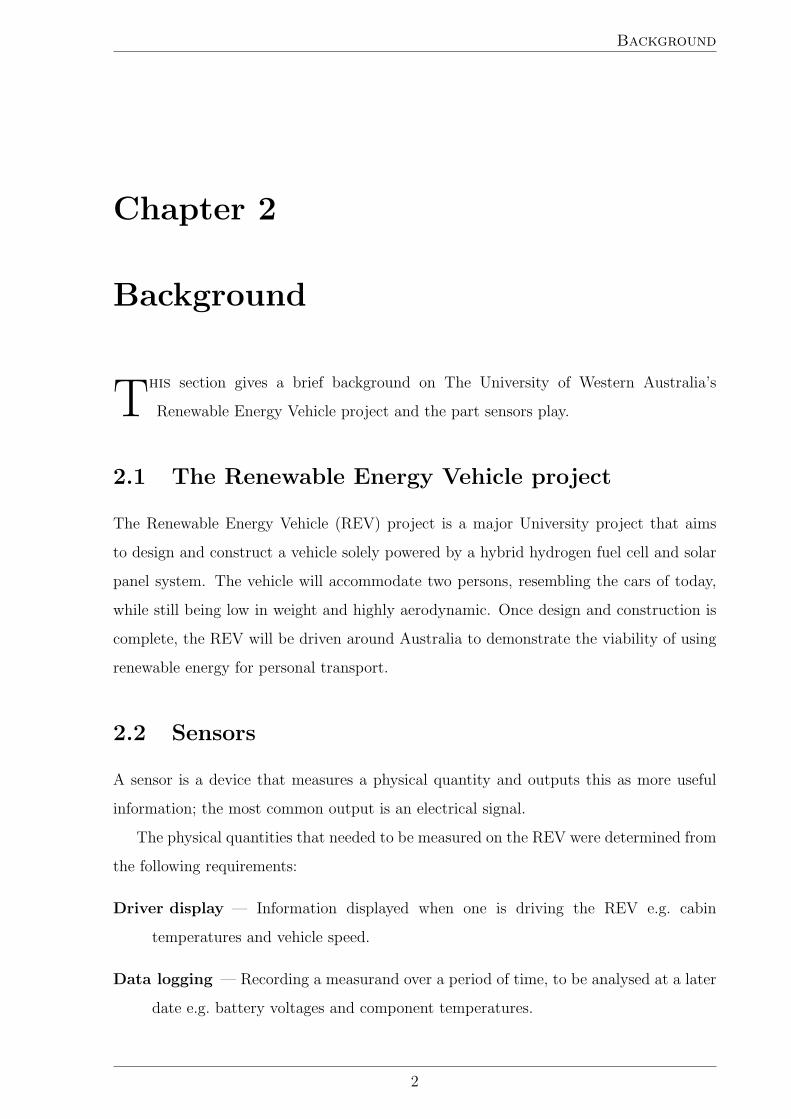
2.4.2 Extreme operating conditions
Extreme operating conditions refers to harsher environmental conditions the sensor would
need to operate in and this is undertaken as a safety precaution. The main concern was
temperature, as this could vary the sensor’s operation greatly. If the sensors cannot
operate in these extreme temperature conditions, then the surrounding temperature will
need to be controlled to accommodate the sensor e.g. cooling fans; their location and size
of inlets/outlets.
2.4.3 Minimise sensor failure
Finally, included in sensor testing are the ways to improve sensor life and minimise the
probability of sensor failure. This can be achieved by simply placing the sensor in an
enclosure to protect the sensor physically and from EMI, or more involved such as how
the sensor will be positioned and fixed in the REV to maximise the sensor’s operation.
This includes positioning the sensor away from noise sources and/or from heat sources.
6

Literature survey
Chapter 3
Literature survey
There is little available literature specifically on the selection of sensors for an
automotive fuel cell application. There is information on some parts of this topic.
Hence, it has been divided into the following sections.
3.1 General sensor selection
The Laboratory for Measurement and Instrumentation at the University of Twente [6]
published a number of articles addressing the sensor selection problem. One of their
projects, named KISIS (Knowledge based Intelligent system for the Selection of Industrial
Sensors) [7], is the development of a computer program that assists a designer with the
selection of sensors for a given measurement problem. Unfortunately, this project has not
been updated since 2002 and the software is still unavailable to the public. However, an
article [8] published by the same research group does define the sensor selection problem
and goes into detail explaining the relation between the measurand and the measurement,
which is useful if the sensors are to be designed.
Energy Source
System Under Consideration
(SUC)s
Transducer Signal Processing
Description of SUCŝ
EnegyStream
Signal ElectricalSignal
Information
Measurement System
Figure 3.1: Sketch of a standard measurement system used whendeveloping KISIS
Figure 3.1 shows the principle of a standard measurement system. The measurands
7

Literature survey
are represented by the variable vector s which is a parameter of the System Under
Consideration (SUC). The object of the measurement system is to obtain an estimate
of the variable s, which is defined as the variable s. In order to obtain information from
the SUC, there must be an exchange of energy. If the SUC radiates a form of energy,
then a transducer can be used to convert this energy into electrical energy (an electrical
signal). If the SUC does not radiate a form of energy, then an energy source must be
provided.
The article “Selection of Sensors” [9] reproduced from “The Handbook of Measuring
System Design” [10] is a free article on sensor selection that is available online. The article
details the sensor selecting process and divides this into the following four main stages.
Requirements — An exhaustive list of information about the future applications, in-
cluding all possible conditions of operation, environmental factors, and specifications
with respect to quality, physical dimensions and costs.
Selecting the measurement principles — All measurement principles are considered
and the optimum principle obtained through the basis of arguments.
Selecting the sensing method — Given a measurement process, a suitable sensing
method is required. Again, all sensing methods are considered and the optimum
selected.
Sensor selection — The final step is the selection of the sensor, which can be decided
by looking at information published by manufacturers.
Though the article provides some good information about the process of sensor
selection, including using the amount of fluid in a container as an example, it is only
after having completed the sensor selection process with the constraints imposed by the
REV that it is realised how irrelevant the above information is. The REV has a major cost
constraint, hence this restricts the sensor selection range. The other major issue is time,
the needed time to complete each stage of the selection process is not feasible, with over
100 individual sensors this will take a considerable amount of time. The article makes a
good general point about sensor selection “Design methods have evolved over time, from
purely intuitive to formal. The basic attitude is still the use of know-how contained in the
minds of people and acquired through experience.” After gaining experience with sensors,
the author agrees with this statement.
8

Literature survey
3.2 Automotive sensors
There are a number of literary works that contain information about the sensors
used in conventional petrol fuelled automobiles. The book “Understanding Automotive
Electronics” [10] has a chapter on the sensors used in petrol fuelled vehicles, it makes an
important statement about sensor selection “The sensors that are available to a control
system designer are not always what the designer wants, because the ideal device may
not be commercially available at acceptable costs”. This statement reiterates the need for
sensor testing.
Similarly, the book titled “Automotive Computer Controlled Systems” [11] has a
chapter on sensors, which gives a good understanding on how sensors in modern cars work.
The book also stresses the topic of sensor diagnostics, discussing diagnostic techniques for
the electrical parts of a car, including sensors.
A brief extract from“Bosch Technical Literature”[12] is on automotive sensors. It gives
a basic understanding of the sensor problem specifically for an automotive application, as
well as providing a list of sensors that would be found in current automobiles.
3.3 Fuel cell vehicles
A number of articles give a view of the sensors required in prototype vehicles that used
fuel cells.
An article [13] published in the “International Journal of Hydrogen Energy” describes
the design and construction of a fuel cell powered electrical vehicle very similar to the
REV. The main difference was the choice of purchasing commercially available components
rather than designing and constructing them. This included the chassis and the fuel cells.
The article does not discuss the choice of sensors, but merely states what was needed.
However, it gives some good statistics which may be useful in determining the capability
of the REV.
One particular article [14] looks at the design and construction of a fuel cell powered
electric bicycle. The design of the fuel cell power bicycle is quite simple when compared
to the REV. However, the bicycle does have all major components of a fuel cell system
including sensors. Actual provided test data including fuel cell efficiency and power-
current and voltage-current curves may be useful in determining the future performance
of the REV.
9

Literature survey
3.4 Measuring problem
“The Measurement, Instrumentation and Sensors Handbook” [15] addresses all issues
of the measurement problem including sensor selection. In the initial chapters, the
measurement problem is explained along with measurement accuracy and measurement
standards. However, the most useful information is the in depth look at all the
common physical quantity measuring systems including displacement, flows and electrical
measurements. The amount of detail that is available for each different measurement
system can be seen in the temperature chapter, where 11 different temperature measuring
sensors are discussed. This book would be extremely helpful when selecting appropriate
sensors for the measurements that have not yet been covered.
“The Mechatronics Handbook” [3] has a section on sensors. Similarly as the previous
book, it looks at the most common measurement principles, but in lesser detail. The
most useful information was its extensive selection criteria. This criteria was used when
selecting the sensors’ performance specifications for the sensors in this thesis.
The “Instrumentation Reference Book” [16] again addresses the general measuring
problem, and hence is divided into instrumentation by application. Included in the book is
a chapter titled “Instrumentation Systems”which provides another view on the measuring
problem and sensor selection.
10

Hydrogen
Chapter 4
Hydrogen
Hydrogen gas is extremely flammable having an EL of 4.1–74.8% by volume in
air. The minimum energy of hydrogen gas ignition in air at atmospheric pressure is
about 0.02 mJ and it has been shown that escaped hydrogen is very easily ignited [17], the
ignition temperature in air is 520–580 C. In high concentrations, hydrogen may exclude an
adequate supply of oxygen to the lungs, causing asphyxiation. Hydrogen gas is colourless,
odourless and insipid, so the victim may be unaware of its presence. It is therefore crucial
that any hydrogen leaks were detected quickly and accurately.
Hydrogen gas does react with oxygen to form water, though this reaction is
extraordinarily slow at ambient temperature. At high temperatures or with an appropriate
catalyst, hydrogen and oxygen gas are highly reactive. The hydrogen concentration in air
at STP is 0.00005%, but hydrogen emissions from lead acid batteries [18] and fossil
fuel burning may result in higher levels. A hydrogen sensor needs to detect over the
general level of ambient hydrogen levels (0.00005%) and in a variety of environments.
Hydrogen gas is the lightest element having a relative density1 of 0.07. This means the
gas is extremely buoyant and will accumulate near the ceiling of an airtight room. Three
hydrogen gas sensors were needed; one general leak detector for the hydrogen testing
workshop and two safety leak detectors in the driver’s cabin and the fuel cell compartment
of the REV.
4.1 Sensing types
There are a number of sensing principles used to detect hydrogen gas, the common
sensing principles are Metal Oxide Semiconductor, Catalytic Bead, Thermal Conductivity,
1Relative density — the ratio between the density of hydrogen gas and that of dry air at STP
11
Hydrogen
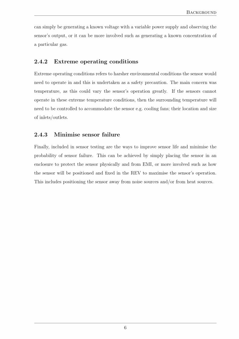
Electrochemical, and Acoustic Wave. Each have their advantages and disadvantages and
these are discussed below.
110
1001000
10000100000
1000000
100 300 500 700
Cost ($)
Sens
ing
Ran
ge (p
pm
MOS (Trace)
MOSCATTCONDECHEMSAW
Figure 4.1: Sensing types and their approximate range and cost [1]
4.1.1 Metal-Oxide Semiconductor
Metal-oxide semiconductor (MOS) sensors are composed of a heater resistor to warm the
sensor to its working temperature (between 200–500 C [19]), and a sensitive resistor made
of a metal-oxide layer deposited on the heater. The electrical resistance of the metal-oxide
layer changes, depending on the temperature and the hydrogen content in the surrounding
air. MOS sensors suffer from several problems including lack of selectivity, stability and
sensitivity, and long response times [20].
4.1.2 Catalytic Bead
Catalytic bead sensors consist of two beads surrounding a wire operating at high
temperatures (450 C). One bead is passivated, so that it will not react when it comes
into contact with hydrogen gas molecules, the other is coated with a catalyst to promote
a reaction with the gas. The beads are generally placed on separate legs of a Wheatstone
bridge circuit (Figure 4.2).
When hydrogen is present there is an increase in resistance on the catalysed bead and
no change on the passivated bead. This changes the bridge balance and changes Vout.
12

Hydrogen
Vsupply
Vout
R2R act
ive
Rrefere
nce
R1
R2
Figure 4.2: Wheatstone bridge circuit, R2 keeps the bridge balanced,R1 and R2 are selected with relatively large resistance values
4.1.3 Thermal Conductivity
Thermal conductivity (TC) sensors are similar to catalytic bead sensors in that they
compare the properties of a sample consisting of hydrogen in air to that of only air, which
is used as a reference. TC sensors work by comparing the thermal conductivity of the
sample to the reference. A heated thermistor is placed in the sample and another as a
reference placed in the reference gas.
If the sample has a higher thermal conductivity than the reference, heat is lost from
the exposed element and its temperature decreases, whilst if the thermal conductivity
is lower than that of the reference, the temperature of the exposed element increases.
Again, a Wheatstone bridge is used to measure the different resistance as a result of the
temperature changes (Figure 4.2).
4.1.4 Electrochemical
Electrochemical sensors work on the same principle as fuel cells. They consist of an anode
and cathode separated by a thin layer of electrolyte. When hydrogen passes over the
electrolyte, a reversible chemical reaction occurs which generates a current, proportional
to the gas concentration. Electrochemical sensors require very little power to operate,
their power consumption is the lowest amongst all sensor types. Electrochemical sensors
have high sensitivity, short reaction time, high reproducibility after calibration, linearity,
zero point stability and relative low cross sensitivity. They are useful in safety and process
control applications. One of the major drawbacks of electrochemical sensors is that the
sensitivity decreases in the course of time, due to the loss of catalytic surface. [21].
13

Hydrogen
4.1.5 Surface Acoustic Wave
Surface acoustic wave (SAW) sensors can be used in a number of applications, such as
gas, fluid and biological sensing. SAW sensors work by creating an acoustic wave on two
surfaces, with a piezoelectric transducer that propagates through the material, where it is
then received by a second piezoelectric transducer that converts it back into an electrical
signal. One surface is coated with a hydrogen reactive film that changes the properties
of the material when hydrogen is present, the other surface is left uncoated and is used
as a reference. This change in properties causes the received acoustic wave to change in
frequency or amplitude, proportional to the concentration of hydrogen [22]. SAW sensors
are reasonably priced, inherently rugged, very sensitive and intrinsically reliable [23].
SAW sensors have been successfully shown to measure hydrogen gas concentrations in an
experimental setup [24][25].
4.2 Sensor Selection
When selecting a hydrogen sensor, the main factors are sensing range, resolution,
operating conditions, and interference gasses. Depending on the sensing range, the data
sheet can either specify the concentration in percent in volume or parts per million (PPM),
where 1% is equal to 10 000PPM. After searching for sensors and obtaining quotes of
$1350 and $3500, the company Neodym Technologies [1] was discovered that produced
hydrogen sensors specifically for fuel cell applications at a low cost.
4.2.1 MiniKnowz
The MiniKnowz is Neodym Technologies’ lowest priced combustible gas sensor between
$68–106, depending on features, and was initially chosen for this reason (Figure 4.3). The
MiniKnowz uses a MOS sensing element, that provides a typical response time of 4–10 s
and a typical accuracy of ±800PPM.
The distinct drawback of this sensor is that the sensor may be permanently damaged
even by brief exposure to extremely high concentrations of hydrogen gas (typically
>5 times the maximum sensing range) [26]. The sensors maximum sensing range is
20 000PPM, meaning any concentrations greater then 10% by volume in air, will cause
damage. This level is not suitable for use in a hydrogen testing workshop where it is
quite possible that these concentrations could occur. It is useful as a driver’s cabin sensor
14

Hydrogen
Sensor head
LED indicator
Figure 4.3: MiniKnowz hydrogen concentration sensor
where any hydrogen will be rare, and used only as a safety measure. Due to its inexpensive
price, the MiniKnowz may be used as a disposable sensor. If a large leak occurred and
the sensor was over exposed, it would go into its error state of 0V, which is different from
its normal working state of 0.5V. The sensor would then either have to be replaced or the
sensor head replaced and the sensor recalibrated.
Interference gas is another concern. Detectors will read accurately in the presence of
homogeneous hydrogen gas/air mixtures, but will also produce readings in the presence
of other inorganic and organic vapours. “Heterogeneous gas mixtures generally have a
synergistic effect on the sensor, and in the absence of a target gas presence, the interference
gases will manifest themselves as ‘false’ readings” [26]. The REV will be subject to various
degrees of hydrocarbons from other vehicles exhaust. When emailed about this, Neodym
Technologies stated “the sensor will pick up the unburnt hydrocarbons from gasoline
engines if it is exposed to the direct exhaust stream. This has not been a problem for
any of our automotive customers to date. Perhaps, because the inside of their fuel cell
enclosures are positively ventilated” [27]. The sensor was tested to observe the effect of
hydrocarbons.
4.2.2 Panterra
The Panterra is a range of gas sensors which use a variety of sensing technologies to sense
a variety of gasses. The distinct advantage over the MiniKnowz is that they can operate
in harsher environmental conditions, but this comes at a higher cost of approximately
$325 per sensor, again depending on options.
The main advantage of the Panterra range is their ability to withstand high
concentrations of hydrogen without permanent damage. This made them suitable as a
general leak detector for use in the hydrogen testing workshop, where high hydrogen
15

Hydrogen
concentrations could occur. Initially, the Panterra-SONIC based on acoustic sensor
technology was chosen due to its large sensing range of 0–100% and inexpensive price,
but was rejected after receiving a reply from Neodym Technologies stating “the sensor is
still in beta and not ready for an automotive application” [27].
The choice of sensor came down to either the Panterra-CAT based on catalytic sensor
technology or the Panterra-TCOND based on thermal conductivity sensor technology. The
Panterra-TCOND has a sensing range of 0–100% and the Panterra-CAT 0–40 000PPM.
The Panterra-TCOND has the advantage that the sensor can be operated in anaerobic
and no-moisture environments, and are not affected by silicones [28], but due to its
larger sensing range has a lower sensing resolution and accuracy when compared to the
Panterra-CAT. It was decided that the Panterra-CAT was the most suitable option due
to its high sensing resolution and accuracy, making it more useful detecting hydrogen
concentrations up to the critical EL, where anything greater is considered dangerous
(Figure 4.4).
Sensor head
LED indicator
Buzzer
Figure 4.4: Panterra-CAT
4.3 Calibration Checking
The only method to check sensor accuracy and proper operation is via exposure of the
sensor to a reference gas concentration, and to measure the sensor’s output voltage.
Neodym Technologies recommends that calibration checking should be performed as often
as is practical, and no less frequently than once every six months [26].
Neodym Technologies’ recommended method for generating calibration test gas
mixtures is to dilute pure target gas with clean, normal air in a leak-free chamber of
fixed, known volume [26]. The full safety procedure can be found in Appendix B. Six
16

Hydrogen
calibration tests were performed with each sensor type and the results can be seen in
Appendix C.
To calculate the actual concentration of hydrogen gas in air, the volume of hydrogen
in the syringe (specified in cubic centimeters) is divided by the container’s volume (in mL)
and then multiplied by 1 000 000. This gives a concentration in part per million. In the
tests, a 1075±1mL container was filled with a 5±0.05 cc syringe of 99.75±0.25% (99.5%
minimum purity) hydrogen. This resulted in a concentration of 4640±63PPM.
Given the sensor’s output voltage (Vout), equation (4.1) was used to calculate the
concentration.
Concentration =(Vout − Voffset)Resolution
StepSize(4.1)
where Concentration = hydrogen concentration [PPM]
Vout = output signal voltage [V]
Voffset = zero offset voltage [V]
StepSize = step voltage [V]
Resolution = sensor resolution [PPM]
4.3.1 MiniKnowz
When observing the test results the obvious feature was the discrete step output,
caused by the MiniKnowz’s analogue to digital convertor, which has a resolution
of 0.0784V. The second feature was the randomness that the values settle at; the
peak voltages range from 0.185±0.04–1.033±0.04V and were a result of the air and
hydrogen not mixing evenly. Using Figure C.1(c) as an example seen in Figure 4.5, the
hydrogen concentration was calculated using the following values; Vout = 1.025±0.04V;
Voffset = 0.5V; StepSize = 0.080V; Resolution = 400PPM.
As a result, a concentration of 2625±400PPM was obtained. This value was lower
than the supposed value of 4640±63PPM, and could be attributed to the following
experimental factors.
• The hydrogen and air was not proportionately mixed in the container creating
pockets of high and low concentrations.
• Due to hydrogen being lighter than air, the hydrogen would always rise to the top
of the container. If the sensor was placed in the middle of the container, inaccurate
measurements would occur.
17

Hydrogen
Maximum1.025 V
Response time4.8 S
Figure 4.5: Example MiniKnowz test (Figure C.1(c))
• The transfer of hydrogen from the cylinder to the container was not 100% efficient,
air may have entered during any part of the transfer.
• The sensor may not have high accuracy. The MiniKnowz has a specified typical
accuracy of ±800PPM and a minimum accuracy of ±2000PPM.
Neodym Technologies did give a manufacturer’s certification of assembly, testing, and
calibration with the sensor. It was therefore assumed that the sensor was calibrated
correctly and it was any of the above factor(s) that caused the discrepancy.
Finally, by observing the sensor reading over time, an approximate response time was
calculated. The syringe was emptied up to two seconds after the data acquisition logging
was started. Hence, it took 4.8±1 s to detect the maximum concentration. This can be
compared with the specified typical response time of 4 s and maximum response time of
10 s.
4.3.2 Panterra-CAT
Taking Figure C.2(e) as an example test result seen in Figure 4.6, the first noticeable
feature was the smaller step sized when compared to the MiniKnowz, which resulted in
a smoother curve. Again, a single test was used to determine the sensed concentration
and response time. The hydrogen concentration was calculated using the following values;
Vout = 0.566±0.00245V; Voffset = 0.1V; StepSize = 0.0049V; Resolution = 40PPM. As
a result, a concentration of 3804±40PPM was obtained. This was quite close to the actual
concentration of 4640±63PPM, and may have been due to the different sensing principle
the Panterra-CAT uses that may measure low concentrations more accurately. Again,
18

Hydrogen
the same experimental factors as above could have contributed to the discrepancy. The
Panterra-CAT has a specified typical accuracy of ±500PPM and a minimum accuracy of
±1000PPM.
Neodym technologies again provided a manufacturer’s certification of assembly,
testing, and calibration with the sensor.
Maximum0.566 V
Response time8.9 S
Figure 4.6: Example Panterra-CAT test (Figure C.2(e))
Finally, the response time was compared with the specifications. Again it was assumed
that the syringe was approximately emptied up to two seconds after the data acquisition
logging was started. By observing the test, a response time of 8.9±1 s was observed. This
was comparable to the specified typical response time of 10 s and maximum response time
of 20 s.
4.4 Cross Sensitivity
Cross-sensitivity refers to the response of a sensor to a gas other than hydrogen. The
main interference gas of concern were the hydrocarbons in car exhaust.
The first test was to observe if car exhaust did cause ‘false’ readings. The same
procedure was used as in Appendix B, except instead of injecting hydrogen gas, car
exhaust was substituted.
Observing the test results found in Appendix C, it was evident that car exhaust did
cause ‘false’ readings on both the MiniKnowz and Panterra-CAT. Using an example from
each sensor type (Figure 4.7 and Figure 4.8), a maximum voltage of 0.68V and 0.17V was
seen for the MiniKnowz and Panterra-CAT respectively. This equated to an incorrectly
19

Hydrogen
Maximum0.686 V
Figure 4.7: Example MiniKnowz test (Figure C.3(d))
Maximum0.17 V
Figure 4.8: Example Panterra-CAT test (Figure C.4(d))
detected concentration of 900±400PPM and 571±40PPM respectively of sensed hydrogen
gas. In conclusion the sensors did cause ‘false’ readings when exposed to car exhaust.
Finally, given that the sensors caused ‘false’ readings when exposed to car exhaust,
it was needed to be determined if the sensors could still be used in the REV. The final
test was to simulate the conditions that would be similar if the sensors were placed in the
REV. The sensors were driven around during peak hours in a vehicle for 10 minutes. Two
slightly different tests were conducted. One exposing the sensors directly to a stream of
external air and one placing the sensor away from this stream of air simulating the actual
position of the sensors in the REV.
In both tests the sensors were extremely close to their zero concentration offsets
(Figure 4.9 and Figure 4.10). The largest voltage change was obtained from the
Panterra-CAT when it was positioned close to the air stream, and this was a maximum
20

Hydrogen
Offset voltage0.5 V
Offset voltage0.1 V
MiniKnowzPanterra
Figure 4.9: Hydrogen sensors positioned close to stream of air
Offset voltage0.5 V
Offset voltage0.1 V
MiniKnowzPanterra
Figure 4.10: Away from air source
voltage of 0.143±0.00245V and corresponded to a concentration of 350±40PPM.
When the sensors were positioned away from the air source, a maximum voltage of
0.114±0.00245V was obtained, which corresponded to a concentration of 117±40PPM
which was insignificant. The slightly larger readings when placed next to the air stream,
may have been a result of the air cooling the sensor head and causing incorrect readings.
Also, the tests were conducted in a commercial petrol vehicle and the vehicle itself may
have contributed to the sensors detecting hydrocarbons which would not be the case if it
was situated in the REV.
However, due to the insignificance of the readings during both tests, the hydrogen
concentration sensors are still suitable for use in the REV. If in fact it did cause a
significant problem, the set voltage that determined a leak, would simply need to be
set greater than the obtained maximum readings.
21

Hydrogen
4.5 Increasing Reliability
There are a number of methods to improve the reliability of the hydrogen concentration
sensors throughout their life. However, the most simple was placing the sensor in a
metal enclosure and this protected the sensor from physical damage and from EMI. Three
aluminium enclosures were purchased for the sensors. Slight modifications were made
to the sensors’ PCB to allow the sensors to fit tightly and holes were created in each
enclosure to allow the sensors’ head to be in contact with the surrounding air (Figure 4.11
and Figure 4.12).
Figure 4.11: MiniKnowz in an aluminium enclosure
Figure 4.12: Panterra-CAT in an aluminium enclosure, the sensinghole is located on the side
In order for the sensors to operate free from error the sensors should be positioned
correctly. Even though the REV design is still in its early stage, the approximate position
22
Hydrogen
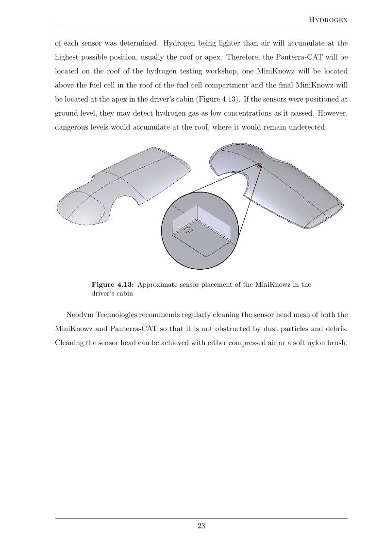
of each sensor was determined. Hydrogen being lighter than air will accumulate at the
highest possible position, usually the roof or apex. Therefore, the Panterra-CAT will be
located on the roof of the hydrogen testing workshop, one MiniKnowz will be located
above the fuel cell in the roof of the fuel cell compartment and the final MiniKnowz will
be located at the apex in the driver’s cabin (Figure 4.13). If the sensors were positioned at
ground level, they may detect hydrogen gas as low concentrations as it passed. However,
dangerous levels would accumulate at the roof, where it would remain undetected.
Figure 4.13: Approximate sensor placement of the MiniKnowz in thedriver’s cabin
Neodym Technologies recommends regularly cleaning the sensor head mesh of both the
MiniKnowz and Panterra-CAT so that it is not obstructed by dust particles and debris.
Cleaning the sensor head can be achieved with either compressed air or a soft nylon brush.
23
Electrical
Chapter 5
Electrical
Electrical measurements include both currents and voltages and were required
for data aquisition (DAQ) and for controlling the REV’s electrical system. For
this reason the measurements needed to have high accuracy and fast response times.
All electrical measurements are already in an electrical signal form that DAQ hardware
accepts. The signals, however, needed to be modified to be compatible with the specific
DAQ hardware. This process is called signal conditioning and can include the processes
of amplification, filtering, electrical isolation and multiplexing. The specifications of the
DAQ hardware that was used is located in Appendix D.
5.1 Voltage
Most DAQ hardware have voltage input ranges of ±10V or ±5V, so higher voltages
cannot be measured directly as it will damage the hardware. Therefore, a voltage sensor
was required to scale the voltage.
The voltages that were to be measured were all DC. This made selecting a suitable
sensor easier. Voltage sensors can be self-powered or externally powered; with self-powered
sensors being referred to as transducers. Most have isolated inputs/outputs which protects
the DAQ hardware. The disadvantages with purchasing a voltage sensor was the lack of
configurability with the input/output ranges. Also, most configurable sensors (convertors)
are considerably expensive.
The cost efficient and more configurable sensor option was to design and build a custom
voltage sensor using common components such as resistors and an operational amplifier
(op-amp).
24
Electrical
5.1.1 Voltage sensor design
3
2
1
out
in
Figure 5.1: Basic voltage attenuator circuit
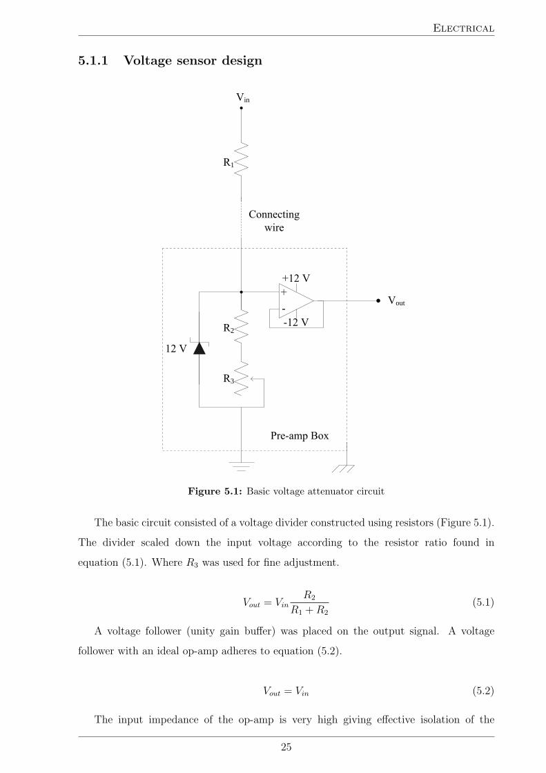
The basic circuit consisted of a voltage divider constructed using resistors (Figure 5.1).
The divider scaled down the input voltage according to the resistor ratio found in
equation (5.1). Where R3 was used for fine adjustment.
Vout = VinR2
R1 + R2
(5.1)
A voltage follower (unity gain buffer) was placed on the output signal. A voltage
follower with an ideal op-amp adheres to equation (5.2).
Vout = Vin (5.2)
The input impedance of the op-amp is very high giving effective isolation of the
25

Electrical
output from the signal source. Very little power is drawn from the signal source avoiding
loading effects [29]. According to National Instruments [30], it is important to select
the proper components to maintain measurement accuracy and performance. Important
considerations for selecting the op-amp included [31]:
• Clean power supply referenced to the analogue input ground
• Using a precision, low-noise op-amp with FET inputs for optimal performance
• The RMS noise added by the new circuitry should be less than the RMS noise of
the DAQ device
• Offset Voltage Drift < 1LSB/C
• Equation (5.3) must hold
R2IB < 1 LSB for desired gain (5.3)
where R2 = source impedance [Ω]
IB = op-amp bias current [A]
The choice of the op-amp was the TL072C produced by STMicroelectronics [32] and
was easily obtained. The TL072C is a low noise JFET input dual op-amp with a maximum
input bios current (IB) of 20 nA and a typical offset voltage drift of 10µV/C.
The DAQ hardware had an input of ±5V with a resolution of 12 bits, where 1 LSB
equated to 2.441±0.0005mV. Given the LSB, the offset voltage drift of the op-amp
(10µV/C) was compared with it and hence was significantly smaller. With the LSB
and the input bios current, equation (5.3) was used to determine the maximum source
impedance (R2). This was calculated as 61±0.5 kΩ which was rounded down to the
standard value of 56 kΩ.
To calculate the value of R3, the resistors’ tolerance (T ) and difference between
calculated and standardised values were taken into account.
R2
R1 + R2
=R2(1± T ) + R3
R1(1∓ T ) + R2(1± T ) + R2
(5.4)
Separating R3,
26

Electrical
R3 =R2R1(1∓ T )
R1
− R2(1± T ) (5.5)
where R1 = standardised R1 value [Ω]
R2 = standardised R2 value [Ω]
T = resistors’ tolerance [%]
Using equation (5.1), R1 was calculated depending on the voltage input. R3 was a
trimpot that allowed precise adjustments and was calculated using equation (5.5). The
standardised values were chosen by rounding down to allow R3 to compensate. If R3 had
an negative value, R2 was needed to be dropped to the next lower standard value and
then R3 recalculated (Table 5.1).
Table 5.1: Examples of voltage range measurements requiredCalculated (kΩ) Standard (kΩ)
Voltage range (V) Ratio R1 R2 R3,1 R3,2 R1 R2 R3
0 – 15 3:1 392 196 55 15 430 180 1000 – 100 20:1 3724 196 45 6 3900 180 500 – 120 24:1 4508 196 44 5 4700 180 50
Finally, a 12V zener diode was placed between the op-amp’s input and ground, and
this protected the op-amp and DAQ hardware in the event of any large voltage entering
the circuit.
Figure 5.2: Constructed voltage sensor
5.1.2 Voltage sensor testing
To conduct tests on the voltage sensor two independent power sources were required. One
to power the op-amp and one to provide an input voltage (Vin). A lab power supply was
27

Electrical
used to provide a variable voltage source between 0–15V. Figure 5.2 shows a constructed
voltage sensor.
Discrete steps
Voltage inVoltage out
Figure 5.3: Voltage sensor calibration, discrete steps were caused whenadjusting the trimpot
The initial test was calibration using the trimpot to ensure Vout was precisely three
times Vin (Figure 5.3). It was very difficult to precisely adjust the trimpot as it was
extremely sensitive and due to it having discrete resistance steps, it meant that it could
not be adjusted to be exactly a third of the input voltage.
Voltage inVoltage out
Figure 5.4: Precise voltage sensor calibration, the right is at higherresolution, enhancing the noise
Instead, a larger potentiometer was used to allow more precise adjustment. After
precise adjustment, at a low resolution Vout and Vin were observed to be overlapping each
other. At a higher resolution, noise was observed (Figure 5.4). This noise may have been
generated from the power supply or was noise detected by the components. The trimpot
and potentiometer may have contributed to the noise as well.
28

Electrical
This potentiometer when precisely adjusted could then be replaced with a fixed
resistor. In this case the value of the potentiometer was 33.2±0.22979Ω and hence it
could be seen why it was difficult to adjust the circuit using a 100 kΩ trimpot. Therefore,
the trimpot could be used for large adjustments but a finer trimpot was needed for more
precise adjustment. This, however, would have resulted in greater complexity in the
sensor design. The other solution was to account for this difference in the software, but
this would defeat the original idea of designing a circuit with Vout and Vin being an integer
multiple ratio.
Voltage inVoltage out
Figure 5.5: Voltage sensor test, Vin manually varied while observingVout
The second test was merely to observe if Vout was a scaler of Vin (Figure 5.5). Vin was
increased/decreased manually between the full range of 0–15V and Vout was observed to
follow, confirming the sensor worked as expected. From observation, the sensor had no
noticeable time delay.
One test done out of interest was to operate the sensor from a single power source
(Vin). This had the benefits of operating as a self-powered sensor, without the need for
the dual polarity power supply. In theory, it should have beeen possible as Vout is never
greater than Vin, but because of the op-amp requiring a negative power supply and the
way the dual polarity power supply operated, it clearly could not operate as a self-powered
unit (Figure 5.6). It would, however, work if Vout was designed to have an offset voltage.
29
Electrical
Voltage inVoltage out
Minimum needed voltage in 2 V
Figure 5.6: Voltage sensor self-powered test
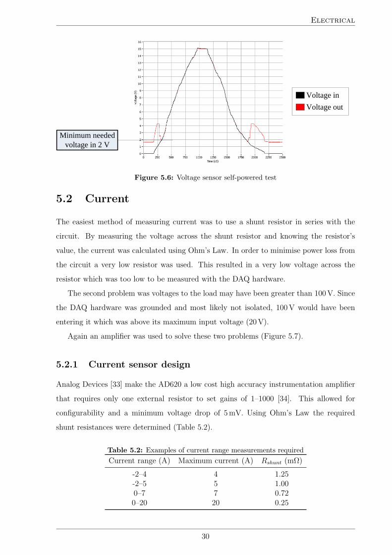
5.2 Current
The easiest method of measuring current was to use a shunt resistor in series with the
circuit. By measuring the voltage across the shunt resistor and knowing the resistor’s
value, the current was calculated using Ohm’s Law. In order to minimise power loss from
the circuit a very low resistor was used. This resulted in a very low voltage across the
resistor which was too low to be measured with the DAQ hardware.
The second problem was voltages to the load may have been greater than 100V. Since
the DAQ hardware was grounded and most likely not isolated, 100V would have been
entering it which was above its maximum input voltage (20V).
Again an amplifier was used to solve these two problems (Figure 5.7).
5.2.1 Current sensor design
Analog Devices [33] make the AD620 a low cost high accuracy instrumentation amplifier
that requires only one external resistor to set gains of 1–1000 [34]. This allowed for
configurability and a minimum voltage drop of 5mV. Using Ohm’s Law the required
shunt resistances were determined (Table 5.2).
Table 5.2: Examples of current range measurements requiredCurrent range (A) Maximum current (A) Rshunt (mΩ)
-2–4 4 1.25-2–5 5 1.000–7 7 0.720–20 20 0.25
30

Electrical
Figure 5.7: Current measurement circuit using a shunt resistor
The required resistances were so small that the wire used to transfer the power could
actually be used as a shunt resistor.
5.2.2 Current sensor testing
To conduct tests, a circuit with a variable current was created. The lab power supply was
capable of a maximum of 5A, so the current sensor was designed for a current range of
0–5A. A 4Ω resistor was used as the load (Figure 5.8).
Figure 5.8: High power-rated resistor used as the load for currenttesting
Using Ohm’s Law the voltage required to produce 5A is 20V, which the lab power
supply was capable of. The power output (in this case 100W) must be lower than the
31
Electrical
resistor’s power rating, which it was. The wire used was flexible 0.75mm2 diameter copper
wire, with a current rating of 7.5A.
R =ρL
A(5.6)
Separating L,
L =RA
ρ(5.7)
where R = resistance of the wire [Ω] (1mΩ)
ρ = resistivity of copper [Ωm] (16.8 nΩm at 20 C [35])
L = required length of the wire [m]
A = cross-section area [m2] (0.75mm2)
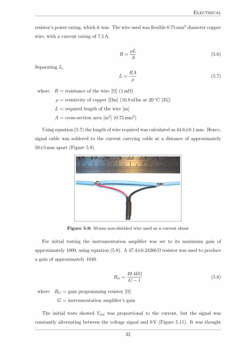
Using equation (5.7) the length of wire required was calculated as 44.6±0.1mm. Hence,
signal cable was soldered to the current carrying cable at a distance of approximately
50±5mm apart (Figure 5.9).
Figure 5.9: 50 mm non-shielded wire used as a current shunt
For initial testing the instrumentation amplifier was set to its maximum gain of
approximately 1000, using equation (5.8). A 47.4±0.24266Ω resistor was used to produce
a gain of approximately 1040.
RG =49.4kΩ
G− 1(5.8)
where RG = gain programming resistor [Ω]
G = instrumentation amplifier’s gain
The initial tests showed Vout was proportional to the current, but the signal was
constantly alternating between the voltage signal and 0V (Figure 5.11). It was thought
32

Electrical
Gain resistor
Figure 5.10: Constructed current sensor, resistor used to program gainshown
that due to amplification of an extremely small voltage (5mV), any noise was amplified
by a factor of approximately 1000 as well. For the next test, shielded cable was used and
the method of joining the signal wire to the current carrying cable was modified.
Figure 5.11: Current sensor test with non-shielded cable
When stripping the insulation from the 24-strand cable to connect the signal wires, it
was extremely difficult not to damage the wires and hence increase the resistance. With
the next test, any wires that may have been accidentally damaged were soldered first
(Figure 5.12 and Figure 5.13).
The test produced some clean looking graphs that were proportional to current but
after 15 s the same alternating signal developed (Figure 5.14).
In order to minimise the possibility of any added noise into the circuit, the dual polarity
power supply which powered the instrumentation amplifier was combined with the current
shunt circuit onto a single professionally printed PCB (Figure 5.15).
With this updated current sensor two independent tests were conducted. One using
the previous 50mm shielded cable and one using 200mm non-shielded cable (Figure 5.16).
33

Electrical
Figure 5.12: 50 mm shielded cable used as a current shunt solderedfirst
Figure 5.13: 50 mm shielded cable used as a current shunt with signalwires attached
Figure 5.14: 50 mm current sensor test with shielded cable
The initial test was to observe if the noise could still be noticed in the circuit. The power
supply was set at a constant voltage and current. The acquired voltage remained fairly
constant with minor spikes occasionally occurring (Figure E.1 and Figure E.2). Hence,
the updated current shunt had removed a significant amount of the alternating behaviour.
The second test was to observe if the voltage output was a multiple of the actual
34

Electrical
Figure 5.15: Combined dual polarity power supply and current shunt
Figure 5.16: 200 mm non-shielded cable used as current shunt
current. The actual current was measured with a multimeter in parallel with the load
circuit and the voltage out was measured using the DAQ hardware. The raw results are
located in Appendix E. The data was plotted and a linear trendline added (Figure 5.17
and Figure 5.18).
y = 0.048948xR2 = 0.993706
-0.05
0
0.05
0.1
0.15
0.2
0 1 2 3 4
Actual current (A)
Sign
al v
olta
ge (V
Figure 5.17: Current shunt test using 50 mm of shielded cable
It was observed that the two plots were quite linear with the 50mm and 200mm shunt
having an R2 value of 0.993706 and 0.999824 respectively. Determining the gradient of
the two trendlines allowed the voltage-current ratio to be determined and it was 0.048948
and 0.249871 respectively. This multiplication factor will need to be implemented in
35

Electrical
y = 0.249871xR2 = 0.999824
0
0.2
0.4
0.6
0.8
1
0 1 2 3 4
Actual current (A)
Sign
al v
olta
ge (V
Figure 5.18: Current shunt test using 200 mm of non-shielded cable
software to convert from the voltage out to actual current. The linearity of each plot
confirmed that the sensor was working as expected. The tests also showed that the initial
calculated length of 50mm that was assumed to equate to 1mΩ was actually 48.948 1µΩ,
approximately 20 times lower. This was probably due to inaccuracies when measuring the
shunt length, and the assumed wires’ diameter may have varied. This very small resistance
may also explain the previous readings when the signal was constantly alternating between
Vout and 0V.
Measuring currents with a shunt resistor was a cost effective method that produced
favourable results. However, problems did arrive when wire was used as the shunt resistor.
If the wire was too short, the instrumentation amplifier measured an extremely small signal
and hence noise interfered with the signal easily. When the wire was extended it acted as
an antenna picking up EMI. This would be a greater problem if the current sensors were
situated around the REV motors which produced large amounts of EMI. The alternative
to using a wire as a shunt is to purchase specifically made shunt resistors, even though
they have the disadvantage of being costly and relatively heavier. However, they can be
designed to be a specific resistance and made to withstand temperature changes which is
beneficial.
5.3 Dual polarity power supply
One of the problems with using an amplifier is the requirement of a dual polarity power
supply. Usually, a simple dual polarity power supply can be made if an AC power source
is available, but since the REV will be solely operating on DC power, an inverting DC-DC
36

Electrical
regulator circuit is required. MAXIM [36] produces the semiconductor MAX636 [37] which
is an inverting switching regulator specifically designed for minimum component DC-DC
conversion in the 5–500mW range (Figure 5.19). Figure 5.20 shows the constructed dual
polarity power supply.
Figure 5.19: Inverting switching regulator based around the MAX636
Figure 5.20: Constructed inverting switching regulator
5.3.1 Testing
The first test was to observe how the dual polarity power supply negative output changed
depending on the received input. The input voltage was set at 0V and the voltage
gradually increased to approximately 12V, which would be the expected voltage in normal
operation. After being steady at approximately 12V the power supply was gradually
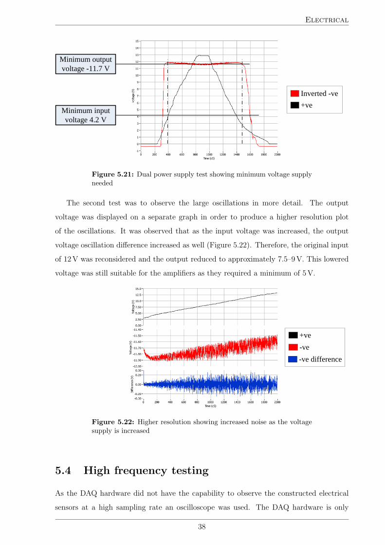
decreased back to 0V (Figure 5.21). It was observed that 4.2V was required for the dual
polarity power supply to reach its minimum output of -11.7V. At the dual polarity power
supply’s minimum, it was observed that the output created large oscillations when the
input was at its max of 12V.
37
Electrical
Minimum input voltage 4.2 V
Minimum output voltage -11.7 V
Inverted -ve+ve
Figure 5.21: Dual power supply test showing minimum voltage supplyneeded
The second test was to observe the large oscillations in more detail. The output
voltage was displayed on a separate graph in order to produce a higher resolution plot
of the oscillations. It was observed that as the input voltage was increased, the output
voltage oscillation difference increased as well (Figure 5.22). Therefore, the original input
of 12V was reconsidered and the output reduced to approximately 7.5–9V. This lowered
voltage was still suitable for the amplifiers as they required a minimum of 5V.
+ve-ve-ve difference
Figure 5.22: Higher resolution showing increased noise as the voltagesupply is increased
5.4 High frequency testing
As the DAQ hardware did not have the capability to observe the constructed electrical
sensors at a high sampling rate an oscilloscope was used. The DAQ hardware is only
38

Electrical
capable of a maximum sampling rate of 50 kHz with a resolution of 2.441mV. However,
the sampling rate was set at only 100Hz in LabVIEW.
The dual polarity power supply was tested first as this was thought to be the source
of the created noise due to its switch mode operation. The dual polarity power supply
was tested without a load. It was observed that the power supply was in fact a saw
wave on the negative output (Figure 5.23). The wave had a frequency of 394.3Hz and a
peak-to-peak voltage of approximately 330mV.
Figure 5.23: Dual power supply test, negative output with no load
However, testing the circuit without a load was not a good representation of the
performance of the circuit. Hence, the dual polarity power supply was connected to the
voltage sensor (Figure 5.24). Operating with a load, placed the sensor under similar
conditions as when connected to the DAQ hardware.
Figure 5.24: Dual power supply test, negative output with load
39

Electrical
Again, a saw wave was observed, but on this occasion it was at a frequency of 1.678 kHz.
The peak-to-peak voltage was approximately the same as the previous tests, at 352mV.
Testing the voltage sensor was mainly to observe if there was any noise that the DAQ
hardware was filtering (Figure 5.25). It was observed that there were large spikes in the
voltage out that were not being detected by the DAQ hardware. The frequency of these
spikes were 60.95 kHz .
Figure 5.25: Voltage sensor test with oscilloscope
Finally, the current sensor was tested with the 50mm and 200mm shunt to determine
the source of the original noise (Figure 5.26). Similar to the voltage sensor test, large
spikes were observed. A minimum and maximum of -0.96V and 8.64V respectively was
calculated with the oscilloscope, and hence these spikes may have been the cause of the
original oscillations detected by the DAQ hardware.
Figure 5.26: Current sensor test with 200 mm shunt, spikes can beobserved
40

Electrical
On closer observation it was observed that these spikes were smooth waves approxi-
mately 1µs in length (Figure 5.27).
Figure 5.27: Current sensor test with 200 mm shunt, zoomed in on asingle spike
Methods for removing these voltage spikes have been discussed in Chapter 7 in the
section on future work.
41

Temperature
Chapter 6
Temperature
There are numerous temperature measurements required for various parts of the
vehicle. These include air temperatures in the driver’s compartment and on
components that have a specific operating temperature, such as motors, electrical
components and the fuel cell.
6.1 Low temperatures
Low temperature measurements (generally between 0 C to 100 C) were the most simple
to implement using integrated-circuit temperature sensors and these could be purchased
easily and inexpensively. Analog Devices [33] make the TMP35 [38] a low voltage,
precision centigrade temperature sensors with a range of 10–125 C. It provides a voltage
output that is linearly proportional to the Celsius temperature.
The sensor’s power supply maximum was 5.5V, so a 5V regulator was used to allow
a larger power voltage range.
TMP35
5 V regulator
Figure 6.1: TMP35 temperature sensor with 5 V regulator on a PCB
42
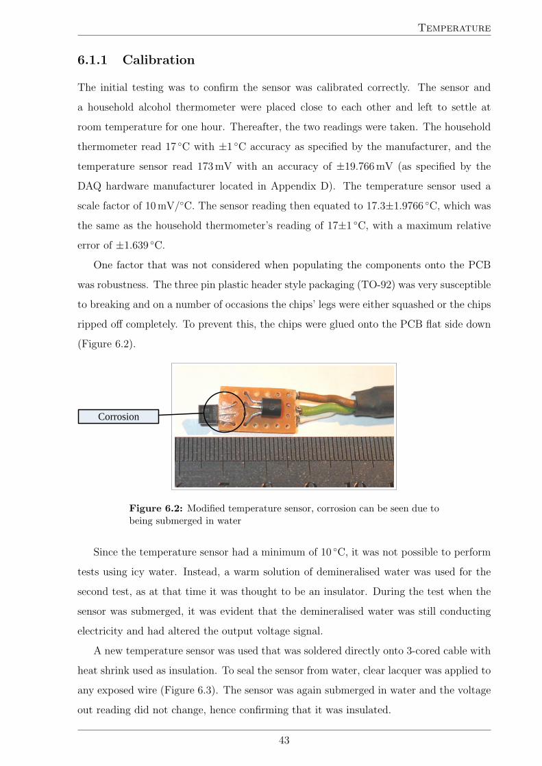
Temperature
6.1.1 Calibration
The initial testing was to confirm the sensor was calibrated correctly. The sensor and
a household alcohol thermometer were placed close to each other and left to settle at
room temperature for one hour. Thereafter, the two readings were taken. The household
thermometer read 17 C with ±1 C accuracy as specified by the manufacturer, and the
temperature sensor read 173mV with an accuracy of ±19.766mV (as specified by the
DAQ hardware manufacturer located in Appendix D). The temperature sensor used a
scale factor of 10mV/C. The sensor reading then equated to 17.3±1.9766 C, which was
the same as the household thermometer’s reading of 17±1 C, with a maximum relative
error of ±1.639 C.
One factor that was not considered when populating the components onto the PCB
was robustness. The three pin plastic header style packaging (TO-92) was very susceptible
to breaking and on a number of occasions the chips’ legs were either squashed or the chips
ripped off completely. To prevent this, the chips were glued onto the PCB flat side down
(Figure 6.2).
Corrosion
Figure 6.2: Modified temperature sensor, corrosion can be seen due tobeing submerged in water
Since the temperature sensor had a minimum of 10 C, it was not possible to perform
tests using icy water. Instead, a warm solution of demineralised water was used for the
second test, as at that time it was thought to be an insulator. During the test when the
sensor was submerged, it was evident that the demineralised water was still conducting
electricity and had altered the output voltage signal.
A new temperature sensor was used that was soldered directly onto 3-cored cable with
heat shrink used as insulation. To seal the sensor from water, clear lacquer was applied to
any exposed wire (Figure 6.3). The sensor was again submerged in water and the voltage
out reading did not change, hence confirming that it was insulated.
43

Temperature
Figure 6.3: TMP35 temperature sensor directly connected to 3-corecable
When both the temperature sensor and household thermometer were submersed in
warm water, the temperature sensor outputted 429.7mV with an accuracy of ±19.766mV,
which equated to 42.97±1.9766 C. This was again the same as the household thermometer
that read 43.5±1 C. There was a maximum relative error of ±1.753 C.
6.1.2 Testing
A number of tests were conducted on the temperature sensors to observe their character-
istics. The first test was to observe their response time. A cup of mineral oil with one
temperature sensor was heated up to 97.2±1.9766 C. The second temperature sensor was
then placed into the oil and its response time was observed to be 37±1 s (Figure 6.4).
Hence, the temperature sensor would not be useful in situations of quick temperature
changes. This, however, would not be a problem as most temperatures in the REV
change gradually.
Response time37 s
with regulatorwithout
Figure 6.4: Response of the temperature sensors when submerged inhot oil
The second test was to observe the sensor’s minimum detection temperature. The
sensor was placed in icy water (approximately 0 C) and the minimum measured
44
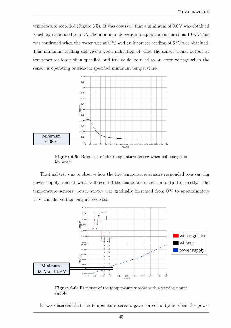
Temperature
temperature recorded (Figure 6.5). It was observed that a minimum of 0.6V was obtained
which corresponded to 6 C. The minimum detection temperature is stated as 10 C. This
was confirmed when the water was at 0 C and an incorrect reading of 6 C was obtained.
This minimum reading did give a good indication of what the sensor would output at
temperatures lower than specified and this could be used as an error voltage when the
sensor is operating outside its specified minimum temperature.
Minimum0.06 V
Figure 6.5: Response of the temperature sensor when submerged inicy water
The final test was to observe how the two temperature sensors responded to a varying
power supply, and at what voltages did the temperature sensors output correctly. The
temperature sensors’ power supply was gradually increased from 0V to approximately
15V and the voltage output recorded.
Minimums3.0 V and 1.9 V
with regulatorwithoutpower supply
Figure 6.6: Response of the temperature sensors with a varying powersupply
It was observed that the temperature sensors gave correct outputs when the power
45

Temperature
supply was at least 3V. At voltages lower than this, ‘false’ readings occurred. Thus,
if there were power supply problems, the sensors could give higher readings than the
actual temperature and may cause components to shut down due to assuming that they
are overheating. However, multiple temperature sensors could be used to prevent these
errors.
6.2 Temperature effect on electrical components
Many components are susceptible to temperature and their characteristics change as the
temperature changes. Tests were conducted on the most common component; resistors,
to observe to what extent temperature affected them.
6.2.1 Resistors
The resistance of resistors change as temperature changes. Through the following test,
the actual resistance change was calculated and used to determine if this would change
sensor readings enough to cause a problem. The test involved testing three different types
of resistors; carbon film, wire wound, and metal film all with approximately the same
resistance (Figure 6.7). The resistors were submerged into white oil (a non-conductive
oil verified with an insulation tester) and the resistance recorded at various temperatures
using a multimeter (Table 6.1).
Carbon film
Metal film
Wire wound
Figure 6.7: Three resistor types used for testing
Due to the resistors having slightly different resistances, the percentage change
was calculated. The room temperature (20.51 C) readings were used as the reference
resistance (Table 6.2). The percentage change per degree Celsius was then plotted
(Figure 6.8).
46
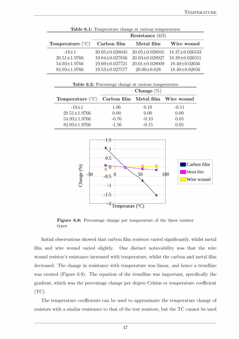
Temperature
Table 6.1: Temperature change at various temperaturesResistance (kΩ)
Temperature (C) Carbon film Metal film Wire wound
-18±1 20.05±0.028045 20.05±0.028045 18.37±0.02653320.51±1.9766 19.84±0.027856 20.03±0.028027 18.39±0.02655154.93±1.9766 19.69±0.027721 20.01±0.028009 18.40±0.0265682.03±1.9766 19.53±0.027577 20.00±0.028 18.40±0.02656
Table 6.2: Percentage change at various temperaturesChange (%)
Temperature (C) Carbon film Metal film Wire wound
-18±1 1.06 0.10 -0.1120.51±1.9766 0.00 0.00 0.0054.93±1.9766 -0.76 -0.10 0.0582.03±1.9766 -1.56 -0.15 0.05
Carbon filmMetal film
Wire wound
-2
-1.5
-1
-0.5
0
0.5
1
1.5
-50 0 50 100
Temperature (°C)
Cha
nge
(%)
Figure 6.8: Percentage change per temperature of the three resistortypes
Initial observations showed that carbon film resistors varied significantly, whilst metal
film and wire wound varied slightly. One distinct noticeability was that the wire
wound resistor’s resistance increased with temperature, whilst the carbon and metal film
decreased. The change in resistance with temperature was linear, and hence a trendline
was created (Figure 6.9). The equation of the trendline was important, specifically the
gradient, which was the percentage change per degree Celsius or temperature coefficient
(TC).
The temperature coefficients can be used to approximate the temperature change of
resistors with a similar resistance to that of the test resistors, but the TC cannot be used
47

Temperature
y = -0.025732x + c
y = -0.002549x + c
y = 0.001671x + c
-3
-2
-1
0
1
2
3
-100 -50 0 50 100 150
Temperature (°C)
Cha
nge
(%) Carbon film
Metal film
Wire wound
Figure 6.9: Percentage change per temperature of the three resistortypes with linear trendline added
Table 6.3: Temperature coefficient of the various resistor typesResistor type Calculated TC (%/C) R2 value
Carbon film −0.025732 0.997339Metal film −0.002549 0.994661
Wire wound 0.001671 0.885916
for different resistances as this changes. The relationship between TC and resistor values
are not linear, and hence will need to be determined by looking at manufacturers’ data
sheets. An example TC plot for carbon film resistors is seen in Figure 6.10. Hence, using
the example TC curve for a 0.25W carbon film resistor, a 20 kΩ resistor had a TC of
−0.033± 0.001%/C when compared with the calculated value of −0.025732%/C it was
quite close. The differences were due to the actual resistors used not being produced by
the same manufacture that produced the plot. However, it did give a good indication of
the expected TC of carbon film resistors.
Taking into account the temperature change, this data can then be used to determine
the effect of temperature on the voltage and current sensors. In both cases a carbon
film resistor was used as an example as they had the highest TC. However, in the actual
design metal film or wire wound would be used. For both sensors an extreme case was
considered, a temperature change of 100 C.
6.2.1.1 Voltage sensor
Resistors were used as the main component of the voltage sensor in the voltage divider
circuit. Assuming that the sensor was perfectly constructed with a Vin:Vout ratio of 1:3
48

Temperature
TC (%
/°C
)
100 1K 10K 100K 1M 10M
0
-0.02
-0.04
-0.06
-0.08
-0.10
-0.12
-0.140
1/4W1/6W1/8W
Resistance (Ω)
Figure 6.10: Example TC plot for carbon film resistors [2]
and hence designed with 392 kΩ and 196 kΩ resistors, having a TC of −0.057%/C and
−0.046%/C respectively. A temperature change of 100 C resulted in modified resistor
values of 369.656 kΩ and 186.984 kΩ respectively. This resulted in a new temperature ratio
of 1.0077:3. Therefore, it affected the voltage divider by approximately 0.77%. Even with
extreme temperature, the change was insignificant.
6.2.1.2 Current sensor
The main concern with the current sensor was the use of the resistor to program
the instrumentation amplifier’s gain. A 47.35Ω resistor was used to produce a gain
of approximately 1044. Hence, the resistor had a TC of −0.0315%/C and with a
temperature change of 100 C resulted in a resistor value of 45.86Ω. This resulted in
a gain of 1078, which was an increase by 3.26%.
6.3 Methods to minimise the effect of temperature
Methods to prevent incorrect values occurring due to temperature changes, include using
the following:
Temperature sensors — These are located around the sensor and updating the sensor
readings in software using a temperature look-up table.
Components that have a low TC — These include wire wound resistors but are
considerably more expensive.
49

Temperature
Temperature compensating circuits — These use two similar components that
cancel any change due to temperature.
Cooling fans — These prevent any large change in temperatures occurring.
50

Conclusions and further work
Chapter 7
Conclusions and further work
Initially the general sensor selection criteria and conditions which included perfor-
mance specifications, operating specifications and costs were discussed. As it is
extremely difficult to find a suitable sensor that matches all criteria, sensor testing is
imperative.
General sensor testing methods were also discussed and these included checking sensor
calibration, testing the sensor under extreme conditions and finally the methods available
to maximise the sensor’s performance. These included placing the sensor in a specific
position to maximise its operation or simply protecting the sensor in an enclosure.
7.1 Measurements discussed
Three different required measuring quantities were looked at and these included hydrogen
concentration, electrical and temperature. These accounted for over 70% of the required
measurements in the REV.
7.1.1 Hydrogen concentration
The hydrogen concentration sensor was required due to safety reasons. Hydrogen would
be needed for testing and running the fuel cell. Hence, it was critical that any hydrogen
leaks were detected.
Three sensors where purchased from the company Neodym Technologies [1] that met
the sensor selection criteria; two MiniKnowzs for the final REV and one Panterra-CAT
for use in the hydrogen testing workshop.
The first tests that were performed on the sensors were calibration checking. A known
51
Conclusions and further work
concentration of hydrogen and air was created and the sensors submerged into it. It was
found that the sensors did output as expected. The second test was initially to observe if
car exhaust caused ‘false’ readings with the sensors, which it did. In order to determine
if the sensors were still useable the sensors were placed inside a car to simulate the REV,
there were no significant readings.
The sensors are suitable for use in the REV. From the tests that were conducted, the
author is confident that the sensors would work as anticipated when finally placed in the
REV.
7.1.2 Electrical
Rather than being purchased the electrical sensors were designed and constructed
specifically for the REV.
The voltage sensors were designed based on a simple voltage divider circuit and a
voltage follower circuit. A design suitable for a maximum voltage of 15V was constructed
and tested. It was observed that it did scale the voltage as expected. The sensor would
be suitable for use in the REV.
The current sensors were based on a shunt resistor measuring the voltage across it
with an instrumentation amplifier. The current sensors showed that they did produce a
voltage signal that was linearly proportional to the current.
7.1.3 Temperature
Simple integrated-circuit temperature sensor were suitable for low temperature measure-
ments. The TMP35 [38] was confirmed to be calibrated correctly and the response times
observed in high and low operating temperatures. The temperature sensors were verified
to work between the temperature range of approximately 6 C to 95 C. Methods of
insulating the sensors from conductive liquids were also discussed. Due to the sensors
being low-priced they are a very simple and effective device for measuring temperatures
around the REV.
The temperature effect on resistors was also tested. Three different types of
resistors were tested and their temperature coefficient calculated. It was found that the
experimental values did agree with the data from manufactures. Finally, it was calculated
to what extent a temperature change of 100 C would affect the current and voltage
sensors if they were designed with carbon film resistors. The voltage sensor input/output
52
Conclusions and further work
ratio was affected by 0.77% and the current sensors gain was affected by 3.26%. Even
at extreme cases, the effect was quite small. Different methods were finally discussed to
minimise sensors’ susceptibility to temperature changes.
7.2 Further work
The sensor tests discussed in this thesis have produced useful information on the sensors’
performance. However, there are a number of tests that can be conducted to determine
further sensor specifications.
7.2.1 Hydrogen concentration
It may be useful to determine the response time of the sensors subjected to higher
concentrations of hydrogen gas. When large leaks occur an extremely fast response time
is needed. However, testing with larger concentrations of hydrogen creates a hazardous
environment.
Similar to the tests conducted with car exhaust, other gases can be used to determine
if they too caused ‘false’ readings. Individually testing the components that constitutes
car exhaust would single out the specific gases that caused ‘false’ readings.
As the REV further develops in design and construction, the precise location of the
sensors and their fixtures could be determined which would also include the method to
remove the sensor for servicing.
7.2.2 Electrical
Due to the REV having a large number of voltage measurements, it may be simpler to
create etched PCBs that consisted of a dual polarity power supply combined with the
voltage sensor. This would minimise any noise being detected on the wires that would
normally connect each other. Multiple op-amps are usually combined onto the single chip,
hence a voltage sensor design could be incorporated where multiple voltage measurements
can be acquired from the single voltage sensor, saving space and weight.
The current sensor’s principle worked as expected. One problem was noise being
detected in the voltage signal. This noise can be minimised by using a specifically designed
shunt resistor that does not vary with temperature and is designed to minimise the amount
53

Conclusions and further work
of detected noise. Further tests should then be conducted to observe if the noise is still
occurring.
There are a number of filtering methods that can be added to the current sensor circuit
to remove the voltage spikes. However, the simplest method is by adding a passive filter
made with capacitors, inductors or resistors. A low-pass filter would be needed to remove
the high frequency spikes.
7.2.3 Temperature
The temperature sensors’ calibration was tested relative to an alcohol thermometer and
then relative to each other. Ideally, a pre-calibrated thermometer should have been used
when checking the sensors’ calibration. This pre-calibrated thermometer should have a
sensing range below 0 C to above 150 C. Due to safety reasons the temperature sensors
were not checked above 100 C as oil at this temperature was hazardous. However, this
could be undertaken in a laboratory environment with the correct apparatus.
The influence of temperature on resistors was discussed. The effect of temperature
change on other components, such as integrated-circuits should also be tested.
7.2.4 General sensor selection
There is still a great deal of work to be done on sensor selection and testing for the REV.
The selection process of the remainder of required sensors (approximately 30%) is almost
finalised, but testing methods still need to be developed and completed. Hopefully, with
the information that has been outlined in this thesis, the job of sensor selection and testing
will be made easier for the REV and any future projects that require sensors.
54

REFERENCES
References
[1] (2005) Neodym Technologies Inc. Vancouver, Canada. [Online]. Available:
http://www.neodymsystems.com
[2] W. C. Limited. (2002) General purpose carbon film resistors. GCF.PDF.
http://www.welwyn-tt.com/pdf/datasheet/GCF.PDF.
[3] R. H. Bishop, The Mechatronics Handbook. CRC Press, 2002.
[4] A. B. of Statistics. (2003) Geography and climate temperature. [Online]. Available:
http://www.abs.gov.au/Ausstats/[email protected]/0/b5186097bad6b76cca256b3400819cd1
[5] (2005) GlobalSpec Inc. Troy, New York. [Online]. Available: http://www.globalspec.
com
[6] (2005) Laboratory for Measurement & Instrumentation. University of Twente, The
Netherlands. [Online]. Available: http://www-mi.el.utwente.nl
[7] (2003) KISIS, Knowledge based Intelligent system for the Selection of Industrial
Sensors. University of Twente, The Netherlands. [Online]. Available: http:
//www.mi.el.utwente.nl/ksn/research/kisis/
[8] M. Korsten, P. van der Vet, and P. Regtien, “A system for the automatic
selection of sensors,” in Proc. IMEKO (International Measurement Confederation)
XVI, Vienna, Austria, Sept. 2000, pp. 211–216. [Online]. Available: http:
//www.mi.el.utwente.nl/ksn/research/kisis/Publications.htm
[9] P. P. Regtien, “Selection of sensors,” in Handbook of Measuring System
Design. John Wiley & Sons, Ltd, 2005, ch. 116. [Online]. Available:
http://eu.wiley.com/legacy/wileychi/hbmsd/pdfs/mm069.pdf
[10] W. B. Ribbens, Understanding Automotive Electronics. Newnes, 1998.
55

REFERENCES
[11] A. W. M. Bonnick, Automotive Computer Controlled Systems. Butterworth-
Heinemann, 2001.
[12] R. Bosch, “Automotive Sensors Basics,” in Bosch Automotive Sensors. Bentley
Publishers, 2005. [Online]. Available: http://www.boschautoparts.co.uk/pdf/
3-934584-50-0.pdf
[13] M. Nadal and F. Barbir, “Development of a hybrid fuel cell/battery powered electric
vehicle,” International Journal of Hydrogen Energy, vol. 21, pp. 497 – 505, 1996.
[14] L. Cardinali, S. Santomassimo, and M. Stefanoni, “Design and realization of a 300
W fuel cell generator on an electric bicycle,” Journal of Power Sources, vol. 106, pp.
384 – 7, 2002.
[15] J. G. Webster, The Measurement, Instrumentation and Sensors Handbook. CRC
Press, 1999.
[16] W. Boyes, Ed., Instrumentation Reference Book. Butterworth-Heinemann, 2003.
[17] Safety Standard for Hydrogen and Hydrogen Systems. Washington DC. [Online].
Available: http://www.hq.nasa.gov/office/codeq/doctree/871916.pdf
[18] A. P. Jardine. (2000) Hydrogen Sensors for Hydrogen Fuel Cell Applications. [Online].
Available: http://www.powerpulse.net/powerpulse/archive/aa 111300a1.stm
[19] P. Riiedi, P. Heim, A. Mortua, E. Franzi, H. Oguey, and X. Arreguit, “Interface
Circuit for Metal-Oxide Gas Sensor,” in Custom Iintegrated Circuits Conference.
Neuchatel, Switzerland: IEEE, 2001.
[20] A. D. Brailsford, M. Yussouff, and E. M. Logothetis, “Theory Of Metal Oxide Gas
Sensors For Measuring Combustibles,” in International Conference on Solid-Safe
Sensors and Actuators. Dearbom, Michigan: IEEE, 1997.
[21] L. Makadmini and M. Horn, “Self-calibrating Electrochemical Gassensor,” in
International Conference on Solid-Safe Sensors and Actuators. Neubiberg,
Germany: IEEE, 1997.
[22] J.F. Vetelino and J.C. Andle and R.S. Falconer, “Theory, design and operation of
surface generated acoustic wave sensors,” Maine, America, 1994.
56

REFERENCES
[23] B. Drafts. (2000, Oct.) Acoustic Wave Technology Sensors. [Online]. Available:
http://www.sensorsmag.com/articles/1000/68/main.shtml
[24] V.I.Anisimkin, “Russia-Italy Researches on Surface Acoustic Wave Gas Sensors,”
Moscow, Russia, 1996.
[25] W. Jakubik and M. Urbanczyk, “Hydrogen detection in Surface Acoustic Wave gas
sensor based on interaction speed,” Gliwice, Poland, 2004.
[26] “MiniKnowz Datasheet,” MiniKnowz Datasheet 100.pdf, 2005. [Online]. Available:
http://www.neodymsystems.com/download/MiniKnowz Datasheet 100.pdf
[27] B. McDonald, private communication, Neodym Technologies Inc., 2005.
[28] “Panterra-TCOND Product Brief,” Panterra-TCOND Brief 100.pdf, 2005. [Online].
Available: http://www.neodymsystems.com/download/Panterra-TCOND Brief
100.pdf
[29] C. R. Nave. (2005) HyperPhysics. [Online]. Available: http://hyperphysics.phy-astr.
gsu.edu/hbase/hph.html
[30] National Instruments. Austin, Texas. [Online]. Available: http://www.ni.com
[31] S. Acosta. (2005) Using a Unity Gain Buffer (Voltage Follower) with a DAQ
Device. [Online]. Available: http://zone.ni.com/devzone/conceptd.nsf/webmain/
CD57A73721E0612586256BAE0055CDD9
[32] (2005) STMicroelectronics. [Online]. Available: http://www.st.com
[33] Analog Devices, Inc. Norwood, Massachusetts. [Online]. Available: http:
//www.analog.com
[34] “AD620 - Low Drift, Low Power Instrumentation Amp with Set Gains of 1 to
10000,” 2004. [Online]. Available: http://www.analog.com/en/prod/0%2C2877%
2CAD620%2C00.html
[35] (2004) Calculation of electrical resistivity with copper. [Online]. Available: http:
//www.allmeasures.com/Formulae/static/formulae/electrical resistivity/12.htm
[36] Maxim Integrated Products, Inc. Sunnyvale, California. [Online]. Available:
http://www.maxim-ic.com
57

REFERENCES
[37] “Preset/Adjustable Output CMOS Inverting Switching Regulators,” 1999. [Online].
Available: http://www.maxim-ic.com/quick view2.cfm/qv pk/1381
[38] TMP35 - Voltage Output Temperature Sensors. Norwood, Massachusetts. [Online].
Available: http://www.analog.com/en/prod/0,,766 811 TMP35,00.html
[39] (2005) BOC Limited. Australia. [Online]. Available: http://www.boc.com.au
[40] (2004) Measurement computing corporation. http://www.measurementcomputing.com.
58

Required measurements on the REV
Appendix A
Required measurements on the REV
Measurement Code Covered
FUEL CELL
Hydrogen pressure cylinder H PRESS CY
Hydrogen pressure in H PRESS IN
Hydrogen flow rate H FLOW
Air pressure A PRESS
Air flow rate A FLOW
Air humidity 1 A HUMD 1
Air humidity 2 A HUMD 2
Air temperature A TEMP X
Water temperature in W TEMP IN X
Water temperature out W TEMP OUT X
Water flow rate W FLOW
Oxygen concentration in O CONC
Stack temperature 1 ST TEMP 1 X
Stack temperature 2 ST TEMP 2 X
Stack temperature 3 ST TEMP 3 X
Stack temperature 4 ST TEMP 4 X
Stack temperature 5 ST TEMP 5 X
Stack temperatures rolling1 (5) ST TEMP R X
Fuel cell voltages rolling (5) CELL V R X
1Rolling — measurements that are not required to be continuously sampled and hence can bemultiplexed together
A1

Required measurements on the REV
Stack current ST I X
Stack voltage ST V X
Hydrogen leak sensor 1 H LEAK 1 X
Hydrogen leak sensor 2 H LEAK 2 X
Hydrogen leak sensor 3 H LEAK 2 X
ELECTRICAL
Capacitor voltage CAP V X
Capacitor current CAP I X
Capacitor current bus CAP I BUS X
Voltage bus V BUS X
Solar voltage 1 SOL V 1 X
Solar voltage 2 SOL V 2 X
Solar voltage 3 SOL V 3 X
Solar voltage 4 SOL V 4 X
Solar voltage 5 SOL V 5 X
Solar current 1 SOL I 1 X
Solar current 2 SOL I 2 X
Solar current 3 SOL I 3 X
Solar current 4 SOL I 4 X
Solar current 5 SOL I 5 X
Net solar current SOL I NET X
Solar current bus SOL I BUS X
Fuel cell current bus FC I BUS X
Right motor current MOTR I X
Right motor phase current A MOTR I A X
Right motor phase current B MOTR I B X
Right motor phase current C MOTR I C X
Right hall effect 1 MOTR H 1
Right hall effect 2 MOTR H 2
Right hall effect 3 MOTR H 3
Left motor current MOTL I X
Left motor phase current A MOTL I A X
Left motor phase current B MOTL I B X
A2

Required measurements on the REV
Left motor phase current C MOTL I C X
Left hall effect 1 MOTL H 1
Left hall effect 2 MOTL H 2
Left hall effect 3 MOTL H 3
12V bad voltage 12VB V X
12V bad current bus 12VB I BUS X
12V bad current 12VB I X
12V stable current bus 12VS I BUS X
Start up battery voltage START V X
Start up battery current START I X
Battery cell voltage rolling (5) BATT V R X
Battery current BATT I X
Electrical temperature 1 E TEMP 1 X
Electrical temperature 2 E TEMP 2 X
Electrical temperature 3 E TEMP 3 X
Electrical temperature 4 E TEMP 4 X
Electrical temperature 5 E TEMP 5 X
Electrical temperature 6 E TEMP 6 X
Electrical temperature 7 E TEMP 7 X
Electrical temperature 8 E TEMP 8 X
Electrical temperature 9 E TEMP 9 X
Electrical temperature 10 E TEMP 10 X
Electrical temperatures rolling (5) E TEMP R X
DYNAMICS
Angular rate roll ANG ROLL
Angular rate pitch ANG PITCH
Inclinometer roll IN ROLL
Inclinometer pitch IN PTCH
Ambient temperature AB TEMP X
Ambient humidity AB HUM
Steering wheel angle ST ANG
Brake pedal BRAKE
Accelerator pedal ACCEL
A3

Required measurements on the REV
Right brake temperature BR TEMP R
Left brake temperature BR TEMP L
Left wheel velocity VEL L
Right wheel velocity VEL R
There are approximately 104 required measurements, 76 of the measuring types have been
covered in this thesis.
A4

Hydrogen concentration sensor testing procedure
Appendix B
Hydrogen concentration sensor
testing procedure
The use of hydrogen for the sensor calibration has been approved by the University’s
Safety & Health Office and a Safety Assessment conducted by the School of Mechanical
Engineering Safety Officer, Rob Greenhalgh (Appendix F).
The testing of sensors requires a known concentration of hydrogen and air mixture
to be generated. This is done in two steps, the first is obtaining a small quantity of
hydrogen gas directly from the cylinder and storing this in a balloon. The second part
involves producing the hydrogen and air mixture.
B.1 Obtaining a quantity of hydrogen
The School of Mechanical Engineering purchases all gases from BOC Australia [39]. BOC
produces three hydrogen types (Table B.1), that are available in two cylinder sizes. Size
D, the smallest available cylinder holds 1.2m3 at STP and size E holds 3m3 at STP.
Ideally the Ultra High Purity would be most suitable as this would create the most
accurate gas mixture, unfortunately due to cost restrictions the Industrial Grade was used
and may have to be used for future testing.
Table B.1: Available hydrogen grades from BOCPrice
Name Minimum Purity Size D Size E
Industrial Grade 99.5% $45.30 $62.02High Purity 99.98% $99.83 $178.36
Ultra High Purity 99.999% $215.17 $219.67
B1
Hydrogen concentration sensor testing procedure
B.1.1 Guidelines for safe hydrogen gas use
Before any hydrogen is used, the tester must
• Familiarise themselves with the MSDS for the chosen hydrogen grade, The MSDS
can be located on BOC’s website.
• Read the Safety Assessment (Appendix F) conducted by the School of Mechanical
Engineering Safety Officer, Rob Greenhalgh.
• Read the following testing procedure thoroughly.
• Complete the Safety Checklist.
When using hydrogen gas, Personal Protective Equipment (PPE) must be worn. PPE
includes:
• Eye protection (safety glasses can be obtained free from the mechanical office)
• Non-sparking clothing (cotton cloths that minimise static buildup)
• Closed toe, non-porous shoes (no thongs or sandals)
Whenever working with hydrogen, all potential ignition sources must be eliminated,
sources of ignition include:
• Open flames (including personnel smoking)
• Electrical equipment
• Static electricity (nylon clothing)
• Heating equipment in buildings
B.1.2 Preparing the cylinder
To order a cylinder of hydrogen, a mechanical workshop staff member must be informed
and must also supervise the use of the cylinder.
Hydrogen cylinders are stored locked up outside the mechanical workshop. Hydrogen
cylinders are always identified as being bright red in colour (Figure B.1). To use the
cylinder it must be moved out of the cage, this increases ventilation and moves the
experiment away from the other stored cylinders. A cylinder trolley designed for the
B2
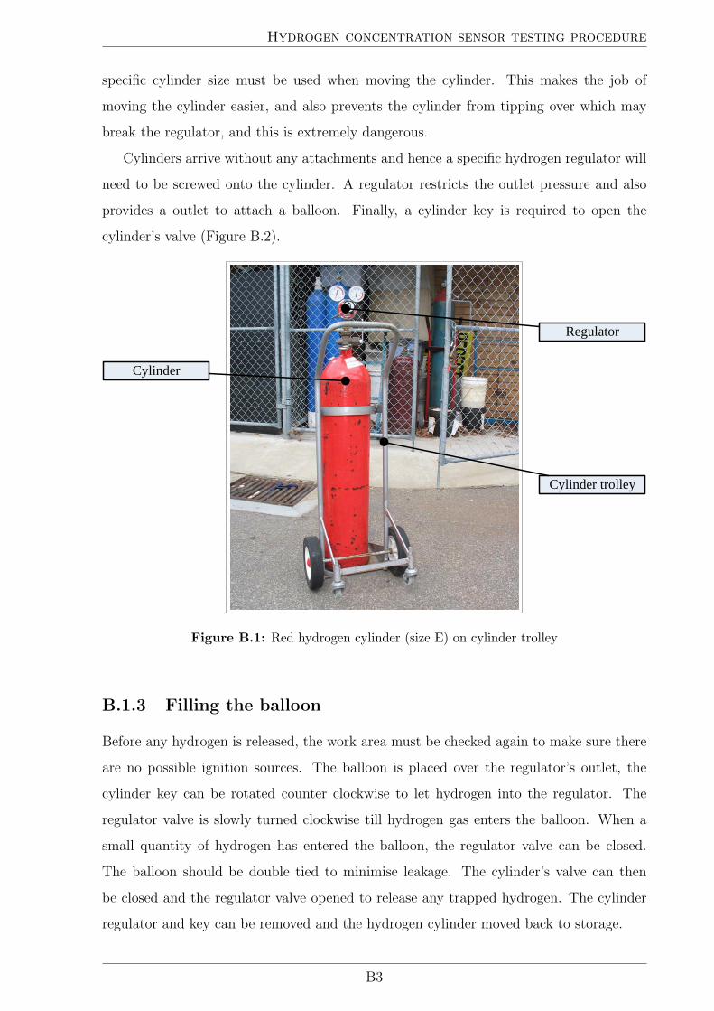
Hydrogen concentration sensor testing procedure
specific cylinder size must be used when moving the cylinder. This makes the job of
moving the cylinder easier, and also prevents the cylinder from tipping over which may
break the regulator, and this is extremely dangerous.
Cylinders arrive without any attachments and hence a specific hydrogen regulator will
need to be screwed onto the cylinder. A regulator restricts the outlet pressure and also
provides a outlet to attach a balloon. Finally, a cylinder key is required to open the
cylinder’s valve (Figure B.2).
Cylinder trolley
Cylinder
Regulator
Figure B.1: Red hydrogen cylinder (size E) on cylinder trolley
B.1.3 Filling the balloon
Before any hydrogen is released, the work area must be checked again to make sure there
are no possible ignition sources. The balloon is placed over the regulator’s outlet, the
cylinder key can be rotated counter clockwise to let hydrogen into the regulator. The
regulator valve is slowly turned clockwise till hydrogen gas enters the balloon. When a
small quantity of hydrogen has entered the balloon, the regulator valve can be closed.
The balloon should be double tied to minimise leakage. The cylinder’s valve can then
be closed and the regulator valve opened to release any trapped hydrogen. The cylinder
regulator and key can be removed and the hydrogen cylinder moved back to storage.
B3

Hydrogen concentration sensor testing procedure
Regulator
Outlet
Cylinder key
Cylinder pressure
Outlet pressure
Open direction
Open direction
Figure B.2: Close up of regulator with valve opening directions
B.2 Creating a calibration gas mixture
Due to hydrogen being lighter then air, accumulation will occur in ceiling spaces and
cavities and can create a severe explosion risk unless adequately vented. Hence the creation
of calibration mixture will be conducted in a fume cabinet.
The fume cabinet documented in this procedure is located in the mechanical
engineering building, room 1.81 (Figure B.3).
The filled hydrogen balloon must be placed under the fume hood and the fume hood
started (Figure B.4).
B.2.1 Creating the hydrogen and air mixture
Before doing any testing with hydrogen the required materials should be obtained
(Figure B.6 and Figure B.5)and the the tester familiarised with the procedure.
B.2.1.1 Materials required
Container — must have an opening large enough for the sensor. Exact volume must be
known, this can be done by filling with water and either measuring the weight or
volume.
Balloons — preferable helium quality. With the necks removed.
B4

Hydrogen concentration sensor testing procedure
Work area
Fume hood Safety screen
Control panel
Figure B.3: Fume hood located in room 1.81
On/Off
Figure B.4: Close up of control panel
Sensor
Multimeter
Battery
Terminal block
Figure B.5: Electrical equipment required for testing procedure
Syringe with needle - can be purchased from pharmacy.
Sensors — located in the REV room, in box marked hydrogen sensors.
Battery — 12V, a drill battery was used in the example.
B5
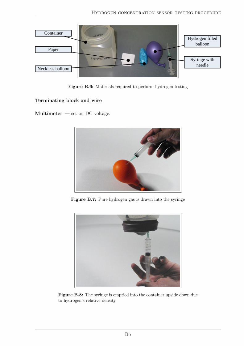
Hydrogen concentration sensor testing procedure
Syringe with needle
Paper
ContainerHydrogen filled
balloon
Neckless balloon
Figure B.6: Materials required to perform hydrogen testing
Terminating block and wire
Multimeter — set on DC voltage.
Figure B.7: Pure hydrogen gas is drawn into the syringe
Figure B.8: The syringe is emptied into the container upside down dueto hydrogen’s relative density
B6

Hydrogen concentration sensor testing procedure
B.2.1.2 Procedure
1. The electrical circuit is setup with all connections secured, in order to prevent
sparking.
2. The sensor is placed into the container and the opening covered with the neckless
balloon.
3. An empty syringe is inserted into the previously filled balloon and pure hydrogen
drawn till the syringe is full (Figure B.7).
4. The full syringe is inserted into the balloon skin covering the opening, and syringe
is emptied (Figure B.8).
5. The container will need to be gently shaken to mix the hydrogen and air. This can
be helped by placing pieces of paper in the container before shaking.
6. Sensor voltage readings are taken.
When sufficient sensor readings have been recorded, any excess hydrogen gas in the
balloons can be released while under the fume hood. The fume hood can be switched off,
and it will go into its shut down cycle.
B7

Hydrogen concentration sensor testing procedure
B.3 Safety checklist
X
PRIOR TO TESTING
Hydrogen testing procedure read
Safety Assessment (Appendix F) read
Personal Protective Equipment obtained
Fume hood room booked
MATERIALS
Hydrogen cylinder
Cylinder attachments (trolley, key and regulator)
Balloons (helium quality)
Container of known volume
Syringe with needle
Hydrogen concentration sensors
Battery (12–48V)
Terminating block and wire
Multimeter
OBTAINING A QUANTITY OF HYDROGEN
PPE worn (safety glasses)
All ignition sources eliminated
Cylinder moved away from cage with trolley
Regulator screwed onto cylinder
Cylinder valve opened
Balloon slightly filled
CREATING A CALIBRATION GAS MIXTURE
PPE worn (safety glasses)
Filled balloons placed under running fume hood
Electrical circuit constructed
Sensor placed into container and covered with neckless balloon
Empty syringe filled with pure hydrogen drawn
Syringe emptied into container
Container gently shaken
Sensor voltage readings measured
Unused hydrogen released
Signed Date
B8

Hydrogen concentration sensor test results
Appendix C
Hydrogen concentration sensor test
results
C1
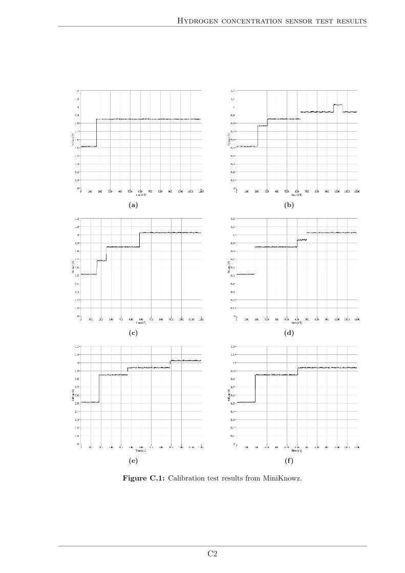
Hydrogen concentration sensor test results
(a) (b)
(c) (d)
(e) (f)
Figure C.1: Calibration test results from MiniKnowz.
C2

Hydrogen concentration sensor test results
(a) (b)
(c) (d)
(e) (f)
Figure C.2: Calibration test results from Panterra-CAT.
C3
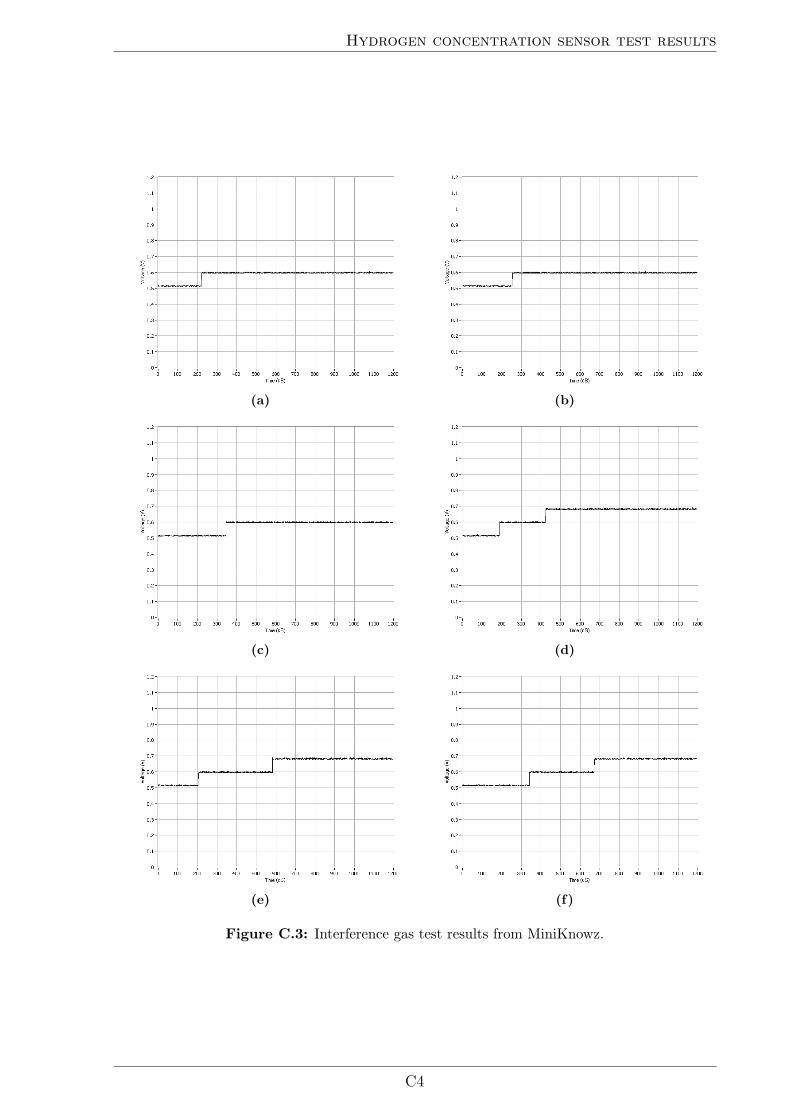
Hydrogen concentration sensor test results
(a) (b)
(c) (d)
(e) (f)
Figure C.3: Interference gas test results from MiniKnowz.
C4

Hydrogen concentration sensor test results
(a) (b)
(c) (d)
(e) (f)
Figure C.4: Interference gas test results from Panterra-CAT.
C5

Test equipment
Appendix D
Test equipment
The following equipment was used to either create a know electrical quantity or to measure
electrical measurements.
D.1 Power supply
The power source that was used for the sensor testing, was a dual channel lab power
supply capable of outputting 0–30V with a maximum current rating of 5A. It was useful
for testing the voltage and current sensors which required a varied voltage in (Vin) and to
also produce 12V for the dual polarity power supply. If a precise voltage was required a
digital multimeter was used, rather than the analogue needles.
In order to determine how ‘clean’ the power supply was, the output was observed with
an oscilloscope (Figure D.1)
Figure D.1: Power supply output viewed with oscilloscope
D1

Test equipment
D.2 Data acquisition hardware
The DAQ hardware used for the majority of testing was the USB-1208FS from Measure-
ment Computing Corporation [40] (Figure D.2). The DAQ hardware specifications of
concern are in Table D.1, Table D.2 and Table D.3.
Figure D.2: The DAQ hardware used for the majority of testing
Table D.1: DAQ general specificationsParameter Specification
Maximum input voltage ±28V maxThroughput software paced 250 S/s typical
Resolution 12 bits
Table D.2: DAQ accuracy at different voltage rangesRange (V) Accuracy (LSB) Accuracy at full scale (mV)
±20 5.1 49.766±10 6.1 29.766±5 8.1 19.766
Table D.3: DAQ noise at different voltage rangesRange (V) LSBrms
±20 0.30±10 0.30±5 0.45
D2

Test equipment
Tests involving the DAQ hardware, were always set on the minimum needed voltage
range i.e. a sensor outputting a voltage of 0–5V was set on the range ±5V, 0–15V required
for a voltage sensor was set on the range ±20V.
D.3 Multimeter
A multimeter was used to measure currents, voltages and resistances. The multimeter used
was the Fluke 170 Series True-RMS Digital Multimeter. The multimeter’s specifications
of concern are in Table D.4.
Table D.4: Multimeter specificationsFunction Resolution Accuracy (±[% of Reading] + [Counts])
DC voltage 0.001V 0.09% + 2DC current 0.001A 1.0% + 3Resistance 0.1Ω 0.9% + 2
D3
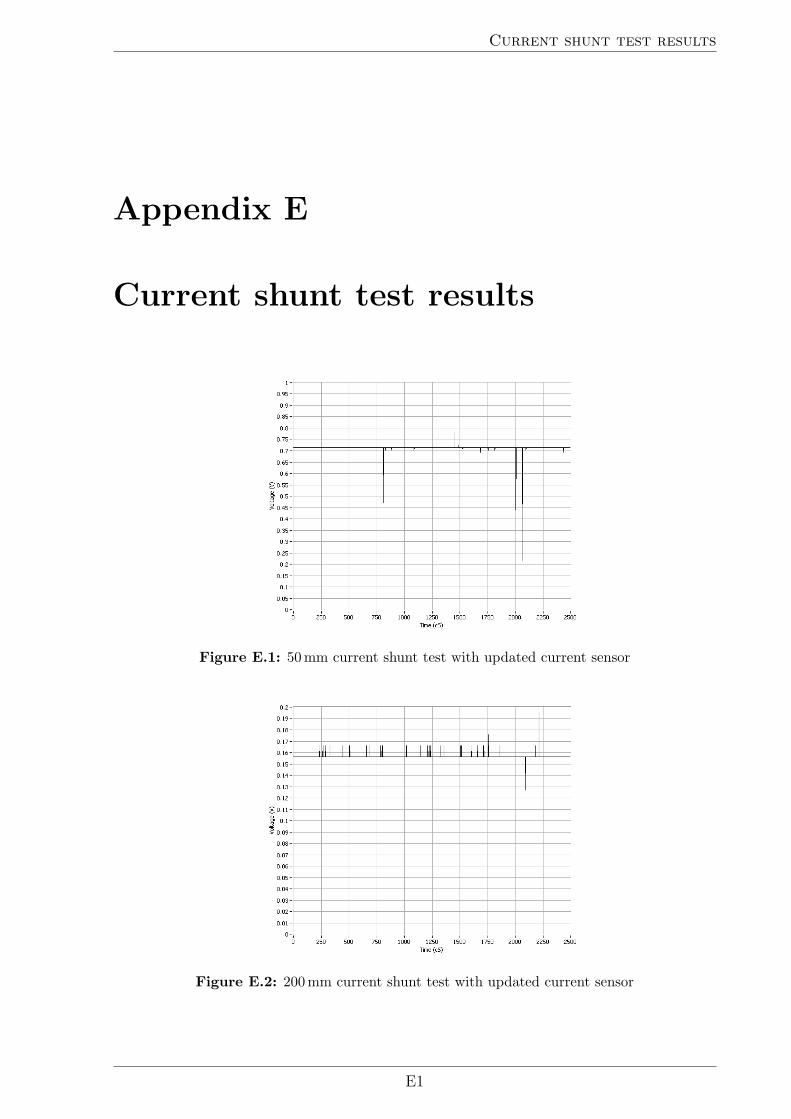
Current shunt test results
Appendix E
Current shunt test results
Figure E.1: 50 mm current shunt test with updated current sensor
Figure E.2: 200 mm current shunt test with updated current sensor
E1

Current shunt test results
Table E.1: Current shunt test using 50 mm of shielded cableActual current (A) Measured voltage (V)
0.11±0.0041 0.02929690.42±0.0072 0.1074220.8±0.011 0.205078
1.27±0.0157 0.3222661.7±0.02 0.429687
1.96±0.0226 0.4882812.34±0.0264 0.5859372.58±0.0288 0.6445312.95±0.0325 0.7324223.29±0.0359 0.820312
Table E.2: Current shunt test using 200 mm of non-shielded cableActual current (A) Measured voltage (V)
0.05±0.0035 00.38±0.0068 0.01953120.61±0.0091 0.02929690.74±0.0104 0.03906250.99±0.0129 0.04882811.07±0.0137 0.0589371.29±0.0159 0.0685941.47±0.0177 0.06835941.65±0.0195 0.0781251.92±0.0222 0.08789062.16±0.0246 0.1074222.31±0.0261 0.1171872.56±0.0286 0.1269532.97±0.0327 0.1464843.29±0.0359 0.15625
E2

STUDENT FINAL YEAR PROJECT - SAFETY ASSESSMENT
Appendix F
STUDENT FINAL YEAR
PROJECT - SAFETY
ASSESSMENT
F.1 PROJECT OUTLINE
Project title ‘Sensors for the Renewable Energy Vehicle’ conducted by Travis Hydzik,
supervisor Associate Professor James Trevelyan.
The requirement of the project is to calibrate a Neodym Technologies hydrogen sensor
according to the organisation’s recommended calibration procedure. The frequency of
calibration is as often as practical and no less than once every six months.
The calibration procedure requires generating a calibration gas mixture of hydrogen and
air in a leak free container of fixed volume.
It is proposed to collect the hydrogen gas from the storage cylinder into a small rubber
balloon (partially inflated). This part of the operation would be carried out in a well
ventilated location, outside the building. The mixing and calibration part of the operation
would be carried out in a laboratory fume cabinet.
Since the volume of hydrogen gas is small and the air/gas concentration very low, below
0.5% and well below the explosive range of hydrogen, the School is permitting this work to
F1

STUDENT FINAL YEAR PROJECT - SAFETY ASSESSMENT
be carried out in a laboratory fume cabinet. The short duration and infrequent calibration
intervals have also been considered in making this decision.
In addition, the proposed calibration method and gas quantities and concentrations
involved have been discussed with Dr. Allan McKinley from the School of Chemistry,
who advises that the proposed method is satisfactory.
F.2 DESCRIPTION OF EXPERIMENTAL PRO-
CEDURE
A small balloon will be filled with hydrogen from the storage cylinder and tied off. This
operation is conducted outside the building.
The remaining operations are conducted in the laboratory fume cabinet.
The sensor will be placed in a 1075ml clean container of air with the opening covered by
a second balloon with the neck removed. An empty syringe is inserted into the balloon
containing hydrogen and 5 cc of gas is drawn off into the syringe. The contents of the
syringe are then transferred into the container, through the second balloon membrane.
The container is then gently shaken to mix the hydrogen and air.
Sensor calibration is then carried out. The test is of approximately 15 minutes duration.
F.3 TASK HAZARD IDENTIFICATION
The proposed calibration routine has been reviewed and the following potential safety
hazards have been identified:
1. Handling and Use of Hydrogen Gas - hydrogen has a wide combustible range
when mixed with air (approximately 4 to 80%). In addition, it is lighter than air
and will accumulate in ceiling spaces and cavities and create a severe explosion risk
unless adequately ventilated.
F2

STUDENT FINAL YEAR PROJECT - SAFETY ASSESSMENT
2. Ignition Sources - potential ignition sources include flames such as cigarettes, and
matches or even sparks generated by electrical devices or static electricity.
3. General Laboratory Hazards - working in a chemical laboratory may expose an
untrained person to other diverse hazards.
F.4 SAFETY CONTROL MEASURES
The Task Hazard Identification indicated the principle hazard associated with this project
is the use of hydrogen. The magnitude of this risk is decreased in the latter stages of
the calibration task, by the low hydrogen/air concentration that is outside the specified
explosive range.
The most hazardous part of the procedure involves the use of the hydrogen storage
cylinder and the mixing procedure, given that the hydrogen concentration may not be
precise, since volume will vary with balloon pressure. There is the requirement to exercise
great care and ensure that there is no opportunity for gas accumulation or ignition sources
to be present.
1. MSDS - A copy of the MSDS for hydrogen must be available and all individuals
involved in handling hydrogen gas must be familiar with its contents.
2. Handling and Use of Hydrogen Gas - The hydrogen cylinder must be stored
and used outside the building. Collection of hydrogen from the cylinder should
involve two people assisting in the operation. This part of the operation should be
carried out when the area is quiet and no ignition sources are present.
3. Mixing Hydrogen and Air - This must be conducted in a fume cabinet, free from
potential ignition sources or other flammable or corrosive substances stored in the
fume cabinet at the same time.
4. Safety Signs - Since the preparation and measurement phase are of short duration,
ensure that only authorised personnel are present in the laboratory at the time. A
Hazard No Entry sign should be displayed on the laboratory door to restrict other
people from entering.
F3

STUDENT FINAL YEAR PROJECT - SAFETY ASSESSMENT
5. Personal Protective Equipment - It is recommended that safety glasses are worn
through the task including use of the fume cabinet sash screen as an additional safety
screen whenever possible. Enclosed footwear is a requirement for all laboratories.
6. On Completion - Ensure that accumulations of hydrogen are removed from all
test apparatus.
7. Working Alone - Since there are some potential hazards associated with this
operation, this work should not be attempted outside of normal working hours.
F.5 MEDICAL SURVEILLANCE AND PERMITS
Not applicable.
F.6 EXPOSURE LIMIT
Not applicable.
F.7 ADVERSE HEALTH EFFECTS
Not applicable.
F.8 PRINCIPLE HAZARDS
Possible explosive gas mixture.
F.9 EMERGENCY PROCEDURES
In the case of injury contact School First Aid Officers or UWA Emergency Services on
2222 if the damage extends to property damage and serious injury. Note the position of
the nearest suitable fire extinguisher in case it is needed.
F4

STUDENT FINAL YEAR PROJECT - SAFETY ASSESSMENT
Safety Assessment conducted by Rob Greenhalgh, School of Mechanical Engineering
Safety Officer, on 18th August 2005.
Acknowledgment and thanks to Dr Allan McKinley (School of Chemistry) for his advice
in addressing safety issue with hydrogen.
F5

Electrical block diagram
Appendix G
Electrical block diagram
The following block diagram gives a indication of the required electrical measurements in
the REV’s electrical system.
G1
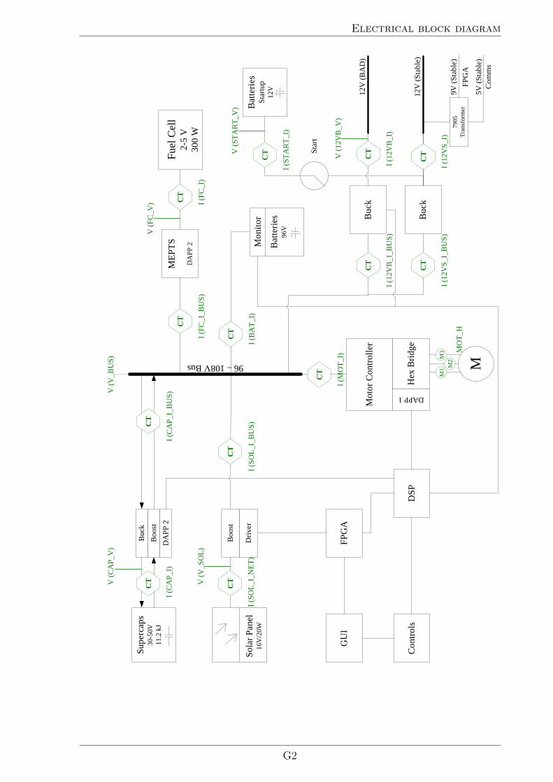
Electrical block diagram
M
Sola
r Pan
el16
V/2
0W
Buc
k
Fuel
Cel
l2-
5 V
300
W
Buc
k
7905
Tran
sfor
mer
MEP
TS
DA
PP 2
Supe
rcap
s30
-50V
11.2
kJ
FPG
A
DSP
Con
trols
Hex
Brid
ge
Mot
or C
ontro
ller
DAPP 1
Boo
stB
uck
DA
PP 2
Boo
st
Driv
er
Bat
terie
s96
V
Mon
itor
Bat
terie
sSt
artu
p12
V
GU
I
Star
t
12V
(BA
D)
12V
(Sta
ble)
9V (S
tabl
e)
Com
ms
I (C
AP_
I_B
US)
CT
I (C
AP_
I)
CT
V (F
C_V
)
V (V
_SO
L)
V (C
AP_
V)
V (V
_BU
S)
V (1
2VB
_V)
V (S
TAR
T_V
)
5V (S
tabl
e)
FPG
A
I (SO
L_I_
NET
)
CT
I (M
OT_
I)
CT M
1 M2M
3 MO
T_H
I (FC
_I)
CT
I (ST
AR
T_I)
CT
I (12
VB
_I)
CT
I (12
VS_
I)
CT
I (SO
L_I_
BU
S)
CT
96 –108V Bus
I (FC
_I_B
US)
CT
I (B
AT_
I)
CT
I (12
VB
_I_B
US)
CT
I (12
VS_
I_B
US)
CT
G2