January, 1995 LIDS- P 2282

Research Supported By:

ARO DAAL03-92-G-0115AFOSR F49620-92-J-2002NSF MIP-9015281

Sensor Array Signal Processing: Two Decades Later*

Krim, H.

Viberg, M.

LIDS-P-2282

January 1995

Sensor Array Signal Processing: Two Decades Later

HAMID KRIM* MATS VIBERG

Stochastic Systems Group Department of Applied ElectronicsMassachussets Institute of Technology Chalmers University of Technology

Cambridge, MA 02139 S-412 96 Gothenburg, Sweden

January 11, 1995

Abstract

The problem of estimating the parameters of superimposed signals using an ar-ray of sensors has received considerable research interest in the last two decades.Many theoretical studies have been carried out and deep insight has been gained.Traditional applications of array processing include source localization and interfer-ence suppression in radar and sonar. The proliferation of estimation algorithms has,however, recently spurred an increasing interest in new applications, such as spatialdiversity in personal communications, medical applications and line detection inimages.

The goal of this manuscript is to provide a brief review of the recent researchactivities in sensor array signal processing. The focus is on estimation algorithms.These are classified into spectral-based and parametric methods respectively, de-pending on the way the estimates are computed. Some of the most well-knownalgorithms are presented, and their relative merits and shortcomings are described.References to more detailed analyses and special research topics are also given.Some applications of sensor array processing methods are also commented upon,and potential new ones are mentioned. The results of real data experiments arealso presented, demonstrating the usefulness of recently proposed estimation tech-niques.

*The work of the first and last authors was supported in part by the Army Research Office (DAAL-03-92-G-115), Air Force Office of Scientific Research (F49620-92-J-2002) and National Science Foundation(MIP-9015281). The second author is supported by AFOSR grant F49620-93-1-0102 and ONR grantN00014-91-J-1967

1 Introduction

Estimation problems in theoretical as well as applied statistics have long been of greatresearch interest given their ubiquitous presence in a great variety of applications. Pa-rameter estimation has particularly been an area of focus by applied statiticians andengineers as problems required ever improving performance [7, 9, 8]. Many techniqueswere the result of an attempt of researchers to go beyond the classical Fourier-limit.

As applications expanded, the interest in accurately estimating relevant temporal aswell as spatial parameters grew. Sensor array signal processing emerged as an activearea of research and was centered on the ability to fuse data from several sensors inorder to carry out a given estimation task. This framework, as will be described in moredetail below, uses to advantage prior information on the data acquisition system (i.e.,array geometry, sensor characteristics, etc.). The methods have proven useful for solvingseveral real-world problems, perhaps most notably source localization in radar and sonar.Other more recent applications are discussed in later sections.

Spatial filtering [6, 42] and classical time delay estimation techniques [8] figure amongthe first approaches to carry out a space-time processing of data sampled at an array ofsensors. Both of these approaches were essentially based on the Fourier transform and hadinherent limitations. In particular, their ability to resolve closely spaced signal sourcesis determined by the physical size of the array (the aperture), regardless of the availabledata collection time and signal-to-noise ratio (SNR). From a statistical point of view, theclassical techniques can be seen as spatial extensions of spectral Wiener filtering [129] (ormatched filtering).

The extension of the time-delay estimation methods to more than one signal' and thepoor resolution of spatial filtering (or Beamformer) together with an increasing numberof novel applications, renewed interest of researchers in statistical signal processing. Itsreemergence as an active area of research coincided with the introduction of the wellknown Maximum Entropy (ME) spectral estimation method in geophysics by Burg [21].This inspired much of the subsequent efforts in spectral estimation, and was intuitivelyappealing as it was reminiscent of the then long-known Yule-Walker autoregressive esti-mation model. This similarity was in spite of the fundamental difference with the latter,which uses estimated covariances, whereas the ME method assumes exact knowledge ofthe auto-covariance function at a limited number of lags. The improvement of the MEtechnique resulted from making minimal assumptions about the auto-covariance functionat lags outside those which are known. Inspired by the laws of physics, Burg proposed tomaximize the entropy of the remaining unknown covariance lags. This improved estima-tion technique, which is readily extended to array processing applications, has been thetopic of study in many different fields, see e.g. [9]. With the introduction of subspace-based techniques [91, 12], the research activities accelerated even further. The subspace-based approach relies on geometrical properties of the assumed data model, resulting ina resolution capability which (in theory) is not limited by the array aperture, providedthe data collection time and/or SNR are sufficiently large.

1These techniques originally used only two sensors.

2

The quintessential goal of sensor array signal processing is to couple temporal andspatial information, captured by sampling a wavefield with a set of judiciously placedantenna sensors. The wavefield is assumed to be generated by a finite number of emitters,and contains information about signal parameters characterizing the emitters. Giventhe great number of existing applications for which the above problem formulation isrelevant, and the number of newly emerging ones, we feel that a review of the area withmore hindsight and perspective provided by time, is in order. The focus is on estimationmethods, and many relevant problems are only briefly mentioned. The manuscript isclearly not meant to be exhaustive, but rather as a broad review of the area, and moreimportantly as a guide for a first time exposure to an interested reader. For more extendedtreatments , the reader is referred to textbooks such as [30, 88, 52, 48].

The balance of this paper consists of the background material and of the basic problemformulation in Section 2. In Section 3, we introduce spectral-based algorithmic solutionsto the signal parameter estimation problem. We constrast these suboptimal solutions toparametric methods in Section 4. Techniques derived from maximum likelihood principlesas well as geometric arguments are covered. In Section 5, a number of more specializedresearch topics are briefly reviewed. In Section 6, a number of real-world problems forwhich sensor array processing methods have been applied are discussed. Section 7 containsa real data example involving closely spaced emitters and highly correlated signals.

3

2 Background and Formulation

This section presents the data model assumed throughout this paper, starting from firstprinciples in physics. We also introduce some statistical assumptions and review basicgeometrical properties of the model.

2.1 Wave Propagation

Many physical phenomena are either a result of waves propagating through a medium(displacement of molecules) or exhibit a wave-like physical manifestation. A wave prop-agation may take various forms, depending on the phenomenon and on the medium. Inany case, the wave equation has to be satisfied. Our main interest, here, lies in the propa-gation of electromagnetic waves, which is clearly exposed through a solution of Maxwell'sequations,

VD = p (1)

VB = 0 (2)0B

VE = (3)

aDVxH = J t' (4)

where D, B, E, H, J respectively denote the electric charge displacement, the magneticinduction, the electric field, the magnetic field and the current density. Equations (1)-(2) express the fact that charges are the sources of electric flux and that there exist nomagnetic charges. The last two equations on the other hand, confirm that a time-varyingmagnetic flux induces a circulation of an electric field and that either a current or adisplacement current causes a circulation of a magnetic field.

Using the conservation of rate of change of charge within a volume V0,

t J Pd3r = J ndS,

with n denoting a surface normal, together with a transform of a surface integral into avolume integral,

V x (V x V) = V(V. V)- V 2 V,

for any vector V, one can derive after some algebra, the fundamental equations of prop-agation:

V(-P)--V2E = - (J + ~t) (5)

-H +At =Jt a(6)-V 2 H + Ea - Vx J. (6)

Solving either of these differential equations (with current charge sources as forcing func-tions) leads to the solution of the other and results in the well-known traveling waveequation,

s(t, p) = s(cxTp - wt),

where w, and ca are respectively the temporal angular frequency and the spatial slownessvector which determines the direction of the wave propagation, and p is the positionvector. The solution for an arbitrary forcing function (i.e. transmitted waveform) isin general obtained as a superposition of single frequencies (narrowband frequencies, e.g.sinusoidals), and often requires a numerical approach. The structure of the above solutionclearly indicates that an exponential-type function coincides with such a behavior. Thepropagating waves we will be focusing on, in this paper, may emanate from sources suchas antennae (E-M waves) or acoustic sources (under water SONAR). The traveling waveequation holds for any application of interest to the estimation methods discussed below.The details of radiating antennae, are left to the excellent book by Jordan [53]. It is alsoclear that homogeneity and time invariance of the fields are assumed throughout.

With little loss of generality2, we will assume a model of an exponential traveling wavesignal,

s(t, p) = s(t- aTp) = ej(wt- kTp), (7)

where w = 27rf is the temporal frequency and k = c/w is the wave-vector. The lengthof k is the spatial frequency (also referred to as the wavenumber), and equals 2-rA, withA being the wavelength of the carrier. In fact, the model we arrive at will be useful alsofor non-exponential signals, provided their bandwidth is much smaller than the centerfrequency3 . This aspect is important, since in many applications the received signals aremodulated carriers. It is also possible that the propagation channel introduces slowlytime-varying phase-shifts and/or amplitude modulations of the received signal, althoughthe transmitted signal is a pure tone.

Equation (7) above clearly shows that the phase variation of the signal s(.) is temporalas well as spatial (as it travels some distance in space). Since the phase is dependentupon the spatial coordinates, the traveling mode (determined by the radiating source)will ultimately dictate how the spatial phase is accounted for. An isotropic point source,as will be assumed throughout, results in spherical traveling waves, and all the pointslying on the surface of a sphere of radius R share a common phase and are referred toas a wavefront. This indicates that the distance between the emitters and the receivingantenna array determines whether or not the sphericity of the wave must be taken intoaccount (near field reception, see e.g. [10]). Far-field receiving conditions implies that theradius R of propagation is so large (compared to the physical size of the array) that a flatplane can be considered, resulting in a plane wave. Though not necessary, the latter willbe our assumed working model for convenience of exposition.

2 As already noted, wideband signals can always be expressed as a superposition of exponential signals.3 More precisely, the narrowband model holds if the inverse bandwidth is much larger than the time

it takes for a traveling wave to propagate across the array.

5

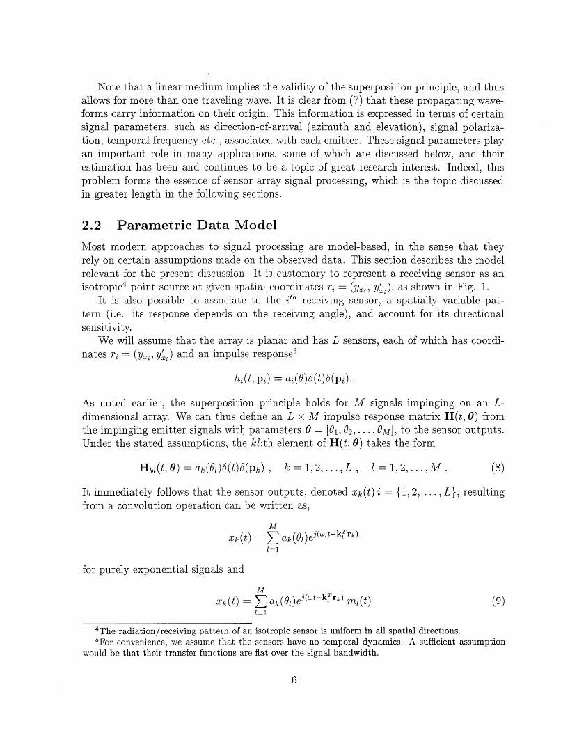
Note that a linear medium implies the validity of the superposition principle, and thusallows for more than one traveling wave. It is clear from (7) that these propagating wave-forms carry information on their origin. This information is expressed in terms of certainsignal parameters, such as direction-of-arrival (azimuth and elevation), signal polariza-tion, temporal frequency etc., associated with each emitter. These signal parameters playan important role in many applications, some of which are discussed below, and theirestimation has been and continues to be a topic of great research interest. Indeed, thisproblem forms the essence of sensor array signal processing, which is the topic discussedin greater length in the following sections.

2.2 Parametric Data Model

Most modern approaches to signal processing are model-based, in the sense that theyrely on certain assumptions made on the observed data. This section describes the modelrelevant for the present discussion. It is customary to represent a receiving sensor as anisotropic4 point source at given spatial coordinates ri = (Yxi, Y'x), as shown in Fig. 1.

It is also possible to associate to the ith receiving sensor, a spatially variable pat-tern (i.e. its response depends on the receiving angle), and account for its directionalsensitivity.

We will assume that the array is planar and has L sensors, each of which has coordi-nates ri = (Yx~, Y'x) and an impulse response5

hi(t, pi) = ai(0)6(t)6(pi).

As noted earlier, the superposition principle holds for M signals impinging on an L-dimensional array. We can thus define an L x M impulse response matrix H(t, 0) fromthe impinging emitter signals with parameters 0 = [01, 02,. . , OM], to the sensor outputs.Under the stated assumptions, the kl:th element of H(t, 0) takes the form

Hkl(t, 0) = ak(O)6(t)6(pk) , k= 1,2,..., L, 1 =1,2,...,M . (8)

It immediately follows that the sensor outputs, denoted k (t) i = {1, 2,..., L}, resultingfrom a convolution operation can be written as,

M

Xk(t) = Zak(l) ej (wl t- k r r k )

1=1

for purely exponential signals and

M

Xk(t) = ak(0l)ej( t - k r ) ml(t) (9)

1=1

4 The radiation/receiving pattern of an isotropic sensor is uniform in all spatial directions.5 For convenience, we assume that the sensors have no temporal dynamics. A sufficient assumption

would be that their transfer functions are flat over the signal bandwidth.

6

Y Sensors

o r

r2 r

0 L2

O O

S 1 S 2

Emitters

Figure 1: General two-Dimensional Array

for narrowband signals. In the latter case, w is the common center frequency of the signalsand ml(t) represents the complex modulation (gain and phase) of the l:th signal, whichby the narrowband assumption is identical at all sensors.

The above equation clearly indicates that the geometry of a given array determinesthe relative delays of the various arrival angles. This is illustrated for the uniform linearand circular arrays in Figure 2, where it is assumed that the array and the emitters areall in the same plane.

The above formulation can be straightforwardly extended to arrays where additionaldimensions provide the flexibility for more signal parameters per source (e.g. azimuth,elevation and polarization). In general, the parameter space can be abstractly representedby some set e and may include all of the aforemetioned parameters. However, most of thetime we will assume that each 01 is a real-valued scalar, referred to as the l:th direction-of-arrival (DOA).

The vector representation of the received signal x(t) is expressed as

x(t) = [a(01), a(0 2),..., a(O)]s(t) = As(t), (10)

7

Uniform Linear Array

Normal source s(t)

0e

Delay Path Length= dsin(O)

d Array AxisReference

source Sensors(t)

Uniform Circular Array

0

k/ 2' IN'j "..-'", Delay Path Length= 7: (R/ X) cos k

Vk =2ir/N(k-1)

R= X/(4sin(r/ L) k

Reference /

Figure 2: Common 2-D arrays

where, with reference to (9),

a(0/) = [al(Ol)ej k rl, a2(O0l)eik r2,. . ,aL(Ol)ejk rL]

s(t) [ewtml(t), ejwtm2(t), ., Cj'MMt)] . (12)

The vector a(01) is referred to as the l:th array propagation vector, and it describes viak rk how a plane wave propagates across the array (note that kl is a function of theDOA) and via ak(0l) how the sensors affect the signal amplitude and phase. In manyapplications, the carrier ejwt is removed from the sensor outputs before sampling.

The received signal, will inevitably be corrupted by noise from each of the receivingsensors, giving rise to the following model asssumed throughout,

x(t) = As(t) + n(t). (13)

The sensor outputs are appropriately sampled at arbitrary time instances, labeled t =1, 2,. . ., N. Clearly, the process x(t) can be viewed as a multichannel random process,

8

whose characteristics can be well understood from its first and second order statisticsdetermined by the underlying signals as well as noise. The sampling frequency is usuallymuch smaller than w, so that x(t) often can be regarded as temporally white.

2.3 Assumptions

The signal parameters which are of interest in this paper, are of spatial nature, andthus require the cross-covariance information among the various sensors, i.e. the spatialcovariance matrix,

R = E{x(t)xH(t)} = AE{s(t)sH(t)}AH + E{n(t)nH(t)} . (14)

Here, the symbol (.)H denotes complex conjugate and transpose (Hermite). Assumingtemporal whiteness and denoting 6t,s the Kronecker delta, the source covariance matrixis defined as

E{s(t)sH(s)} = P t, (15)

whereas the noise covariance matrix is modeled as given by

E{n(t)nH(s)} = 2 16t,s . (16)

Thus, it is assumed that the noise have the same level a2 in all sensors, and is uncorrelatedfrom sensor to sensor. Such noise is usually termed spatially white, and is a reasonablemodel for e.g. receiver noise. However, other man-made noise sources need not resultin spatial whiteness, in which case the noise must be pre-whitened. More specifically,if the noise covariance matrix is Q, the sensor outputs are multiplied by Q-1/2 (Q1/2denotes a Hermitean square-root factor of Q) prior to further processing. The sourcecovariance matrix, P is often assumed to be nonsingular (a rank-deficient P, as in thecase of temporally coherent signals, is discussed in Sections 3.3 and 4).

In the later development, the spectral factorization of R will be of central importance,and its positivity guarantees the following representation,

R = APAH + a 2I = UAUH, (17)

with U unitary and A = diag{A 1, A2, - *, AL} a diagonal matrix of real and positive eigen-values, such that A1 > A2 > ... > AL. Observe that any vector orthogonal to A is an eigen-vector of R with the eigenvalue u2. There are L - M linearly independent such vectors.Since the remaining eigenvalues are all larger than u 2, we can split the eigenvalue/vectorpairs into noise eigenvectors (corresponding to eigenvalues AM+1 = ... = AL = u2) andsignal eigenvectors (corresponding to eigenvalues A1 > ... > AM > or2 ). This results inthe representation

R = USASUfY + UA+ U nH, (18)

where the columns of the signal subspace matrix U, are the M principal eigenvectors,and the noise subspace matrix Un contains the eigenvectors corresponding to the multipleeigenvalue ar2, i.e. An = U2I. Since all noise eigenvectors are orthogonal to A, the columns

9

of Us must span the range space of A whereas those of U, span its orthogonal complement(the nullspace of AH). The projection operators onto these signal and noise subspacesare defined as

I = U UH =A(AHA)-lAH

II' = UnU n = I- A(AHA)-1AH, (19)

which clearly satisfyI = I + l'. (20)

2.4 Problem Definition

The problem of central interest herein is that of estimating the DOAs of emitter signalsimpinging on a receiving array, when given a finite data set {x(t)} observed over {t =1, 2, . .. , N}. As noted earlier, we will primarily focus on reviewing a number of techniquesbased on second-order statistics of data.

All of the earlier formulation assumed the existence of exact quantities, i.e. infiniteobservation time. It is clear that in practice sample estimates are only possible and aredesignated by a-. The ML estimate of R is given by6,

R E X(t)XH (t). (21)N=l

A corresponding eigen-representation similar to that of R is defined as

R= UsAsTUH + UnAnUn. (22)

This decomposition will be extensively used in the description and implementation of thesubspace-based estimation algorithms. Throughout the paper, the number of underlyingsignals, M, in the observed process is considered known. There are, however, good andconsistent signal enumeration techniques available [124, 93, 29, 61] in the event that suchan information is not available, see also Section 5.1.

In Sections 3 and 4, for space reasons, we limit the discussion to the best knownestimation techniques, respectively classified as Spectral-Based and Parametric methods.With the full knowledge of existence of a number of good variations which address par-ticular problems of those described here, the reference list attempts to cover a portion ofthe gap which clearly can never be filled.

6 Strictly speaking, (21) does not give the ML estimate of the array covariance matrix, since it does notexploit its parametric structure. See Section 4 for further details on this aspect. The sample covariancematrix (21) is sometimes referred to as an unstructured ML estimate.

10

3 Spectral-Based Algorithmic Solutions

As pointed out earlier, we classify the parameter estimation techniques into two maincategories, namely the spectral-based and the parametric approaches. In the former, oneforms some spectrum-like function of the parameter(s) of interest, e.g. the DOA. Thelocation of the highest (separated) peaks of the function in question are taken as theDOA estimates. The parametric techniques, on the other hand, require a simultaneoussearch for all parameters of interest. While often more accurate, the latter approach isusually more computationally complex.

The spectral-based methods in turn are divided into the beamforming approaches andthe subspace-based methods.

3.1 Beamforming Techniques

The first attempt to automatically localize signal sources using antenna arrays was throughbeamforming techniques. The idea is to "steer" the array in one direction at the time andmeasure the output power. The locations of maximum power yield the DOA estimates.The array is steered by forming a linear combination of the sensor outputs

L

y(t) = E_ w*xi(t) = wHx(t) , (23)i=l

where (.)* denotes complex conjugate. Given samples y(1),y( 2),...,y(N), the outputpower is measured by

1 N 1 NP(w): =N E y(t) 2 wHx(t)X(t)xH(t)w = wH (24)

t=l t=1

where R is defined in (21). Different beamforming approaches correspond to differentchoices of weighting vector w. For an excellent review of the utility of beamformingmethods, we refer to [115].

3.1.1 Conventional Beamformer

Following the development of the Maximum Entropy criterion formulated by Burg [21] inspectral analysis, a plethora of estimation algorithms appeared in the literature, each usinga different optimization criterion. For a given structured array, the first algorithm whichprecedes even the entropy-based algorithm, is one which maximizes its output power fora certain input. Suppose we wish to maximize the output power from a certain direction0. The array output, assuming a signal at 0 corrupted by additive noise, is given by

x(t) = a(0)s(t) + n(t)

The problem of maximizing the output power is then formulated as

max Efw X(t)Xt)wj = maxw E{X(t)xH (t)}w

- max {E s(t) 2 wHa(0) + 2 W2} (25)

where the assumption of spatially white noise is used in the last equality. Employinga norm constraint on w to ensure a finite solution, we find that the maximizing weightvector is given by

WBF = a(O). (26)

The above weight vector can be interpreted as a spatial filter, which has been matchedto the impinging signal. Intuitively, the array weighting equalizes the delays experiencedby the signal on various sensors to maximally combine their contributions. Figure 3illustrates this point.

d , - - - - -- - ' - source s(t)

d ,c--- >,

\/ Receiving Sensor

6 26 1 365 4 56 6=co

y(t)

Figure 3: Standard Beamformer

Inserting the weighting vector (26) into (24), the classical spatial spectrum is obtainedas

PBF(O) = a H(O)Ra(0) (27)

12

For a uniform linear array (ULA), the steering vector a(O) takes the form (see Figure 2)

a(O) = [i, eim,. , e.(L.1jT , (28)

where

-= -- d sin(8) (29)Cis termed the electrical angle. Here, w is the center frequency of the signals, c is the speedof propagation, d is the inter-element separation and the DOA 0 is taken relative to thenormal of the array. By inserting (28) into (27), we obtain PBF(O) as the spatial analogueof the classical periodogram in temporal time series analysis, see e.g. [83]. Unfortunately,the spatial spectrum suffers from the same resolution problem as does the periodogram.The standard beamwidth for a ULA is 5B = 27/L, and sources whose electrical anglesare closer than /B will not be resolved by the conventional beamformer, regardless of theavailable data quality.

3.1.2 Capon's Beamformer

In an attempt to alleviate the limitations of the above beamformer, such as its resolvingpower of two sources spaced closer than a beamwidth, researchers have proposed numerousmodifications. A well-known method was proposed by Capon [23], who formulated analgorithm as a dual of the beamformer. The optimization problem was posed as

min P

subject to wHa(0) = 1.

Hence, Capon's beamformer attempts to minimize the power received from noise andany signals coming from other directions than 0, while maintaining a fixed gain in the"look direction" 0. The optimal w can be found using, e.g., the technique of Lagrangemultipliers, resulting in

WCAP = H(0) (30)aH ()R-la(0)

The above weight in turn leads to the following "spatial spectrum" upon insertion into(24)

PCAP() - aH(0)R-la(0) (31)

It is easy to see why Capon's beamformer outperforms the more classical one, as theformer uses every single degree of freedom to concentrate the received energy along onedirection, namely the bearing of interest. The Capon beamformer is allowed to giveup some noise suppression capability to provide a focused "nulling" in the directionswhere there are other sources present. The spectral leakage from closely spaced sourcesis therefore reduced, though the resolution capability of the Capon beamformer is stilldependent upon the array aperture.

13

A number of alternative methods for beamforming have been proposed, addressingvarious issues such as partial signal cancelling due to signal coherence [128] and beamshaping and interference control [41, 20, 115].

3.2 Subspace-Based Methods

Many spectral methods in the past, have implicitly called upon the eigen structure ofa process to carry out its analysis (e.g. Karhunen-Loeve representation). One of themost significant contributions came about when the eigen-structure of a process wasexplicitly invoked, and its intrinsic properties were directly used to provide a solution toan underlying estimation problem for a given observed process.

Early approaches involving invariant subspaces of observed covariance matrices includeprincipal component factor analysis [49] and errors-in-variables time series analysis [58]. Inthe engineering literature, Pisarenkos work [81] in time series analysis was among the firstto be published. However, the tremendous interest in the subspace approach is mainlythe result of the introduction of the MUSIC (Multiple SIgnal Classification) algorithm[91, 12].

3.2.1 The MUSIC Algorithm

As noted in Section 2.3, the structure of the exact covariance matrix together with thespatial white noise assumption implies that its eigendecomposition can be expressed as

R = APAH + a2I = UsAsUH + a2 UnUH, (32)

where the diagonal matrix As contains the M largest eigenvalues (assuming APAH to beof full rank). Since the eigenvectors in U, (the noise eigenvectors) are orthogonal to A,we have

Un a(O)= 0, 0C{01,..., M}. (33)

To allow for unique DOA estimates, the array is usually assumed to be unambiguous;that is, any collection of L steering vectors corresponding to distinct DOAs qk forms alinearly independent set {a(rh),...,a(ru,)}. In particular, a ULA can be shown to beunambiguous if the DOAs are confined to -ir/2 < 0 < 7r/2 and d < A/2. Under thisassumption, 01,..., 0M are the only possible solutions to the relation (33), which couldtherefore be used to locate the DOAs exactly.

In practice, as previously noted, an estimate of the covariance matrix R is obtained,and its eigenvectors are split into the signal and noise eigenvectors as in (22). The or-thogonal projector onto the noise subspace is estimated as

--= Uj *UH (34)

The MUSIC "spatial spectrum" is then defined as

aH(()a(O)PM((0) = H(0)a(0) (35)

aH(0)14 a(0)

14

(the denominator in (35) is included to account for non-uniform sensor gain and phasecharacteristics). Although PM(0) is not a true spectrum in any sense (it is merely the dis-tance between two subspaces), it exhibits peaks in the vicinity of the true DOAs provided[IL is close to IIl .

The performance improvement of this method was so significant that it became analternative to most existing estimators. In particular, it follows from the above reasoningthat estimates of an arbitrary accuracy can be obtained if the data collection time issufficiently long or the SNR is adequately high. Thus, in contrast to the beamformingtechniques, the MUSIC algorithm provides statistically consistent estimates. Though theMUSIC function (35) does not represent a spectral estimate, its important limitationis still the failure to resolve closely spaced signals in small samples and at low SNR.This loss of resolution is more serious for highly correlated signals. In the limiting caseof coherent signals7, the property (33) no longer holds and the method fails to yieldconsistent estimates, see e.g. [60]. The mitigation of this limitation is an important issueand is separately addressed at the end of this section.

3.2.2 Extensions to MUSIC

The MUSIC algorithm spawned a significant research activity which led to a multitude ofproposed modifications. These were attempts to improve/overcome some of its shortcom-ings in various specific scenarios. The most notable was the unifying theme of weightedMUSIC which, for different W, particularized to different algorithms,

PWM(0) = aH (0)f a() (36)aH (0)±Wa(0)

The weighting matrix W is introduced to take into account (if desired) the influenceof each of the eigenvectors. It is clear that a uniform weighting of the eigenvectors,i.e. W = I, results in the original MUSIC method. As shown in [99], this is indeed theoptimal weighting in terms of yielding estimates of minimal asymptotic variance. However,in difficult scenarios involving small samples, low SNR and highly correlated signals, acarefully chosen non-uniform weighting may still improve the resolution capability of theestimator (see Section 7).

One particularly useful choice of weighting is given by [62]

W el eT , (37)

where el is the first column of the L x L identity matrix. This corresponds to the Min-Norm algorithm, originally proposed by Tufts and Kumaresan [64, 113] for ULAs andextended to arbitrary arrays in [66]. As shown in [55], the Min-Norm algorithm indeedexhibits a lower bias and hence a better resolution than the original MUSIC algorithm.

7Two signals are said to be coherent if one is a scaled version of the other.

15

3.2.3 Resolution-Enhanced Spectral Based Methods

The MUSIC algorithm is known to enjoy a property of high accuracy in estimating thephases of the roots corresponding to DOA of sources. The bias in the estimates radii [62],however, affects the resolution of closely spaced sources when using the spatial spectrum.

A solution first proposed in [13], and later in [37, 19], is to couple the MUSIC algorithmwith some spatial prefiltering, to result in what is known as Beamspace Processing. Thisis indeed equivalent to preprocessing the received data with a predefined matrix T, whosecolumns can be chosen as the steering vectors for a set of chosen directions:

z(t) = THx(t) . (38)

Clearly, the steering vectors a(O) are then replaced by THa(0) and the noise covariancefor the beamspace data becomes o2 THT. For the latter reason, T is often orthogonalizedbefore application to x(t).

It is clear that if a certain spatial sector is selected to be swept (e.g. some priorknowledge about the broad direction of arrival of the sources may be available), one canpotentially experience some gain, the most obvious being computational, as a smallerdimensionality of the problem usually results. It has, in addition, been shown that thebias of the estimates is decreased when employing MUSIC in beamspace as opposed tothe "element space" MUSIC [37, 137]. As expected, the variance of the DOA estimates isnot improved, but a certain robustness to spatially correlated noise has been noted in [37].The latter fact can intuitively be understood when one recalls that the spatial pre-filterhas a bandpass character, which will clearly tend to whiten the noise.

Other attempts to improving the resolution of the MUSIC method are presented ine.g. [56, 33, 135], based on different modifications of the criterion function.

3.3 Coherent Signals

Though unlikely that one would deliberately transmit two coherent signals from distinctdirections, such a phenomenon is not uncommon as either a natural result of a multipathpropagation effect, or intentional unfriendly jamming. The end result is a rank deficiencyin the source covariance matrix P. This, in turn, results in a divergence of a signaleigenvector into the noise subspace. Therefore, in general UHa(O) : 0 for any 0 and theMUSIC "spectrum" may fail to produce peaks at the location of DOAs. In particular,the ability to resolve closely spaced sources is dramatically reduced for highly correlatedsignals, see. e.g. [63].

In the simple case of two coherent sources being present and a uniform linear array,there is a fairly straightforward way to "de-correlate" the signals. The idea is to employa forward-backward (FB) averaging as follows. Note that a ULA steering vector (28)remain unchanged, up to a scaling, if its elements are reversed and complex conjugated.More precisely, let J be an L x L exchange matrix, whose components are zero exceptsfor ones on the anti-diagonal. Then, for a ULA it holds that

Ja*(O) = e-j(L-l)4a(e) . (39)

16

The so-called backward array covariance matrix therefore takes the form

RB = JR*J = A -(L-)PV-L-l)AH + o2 I , (40)

where · is a diagonal matrix with ejhk, k = 1, ... , M on the diagonal. By averaging theusual array covariance and RB, one obtains the FB array covariance

RFB = (R + JR*J)

= AAH + 2 I (41)

where the new "source covariance matrix" P - (P + ~-(L-)Pq>-(L-1))/2 generically hasfull rank. The FB version of any covariance-based algorithm simply consists of replacingR with RFB, defined as in (41). Note that this transformation has also been used innoncoherent scenarios, and in particular in time series analysis, for merely improving thevariance of the estimates.

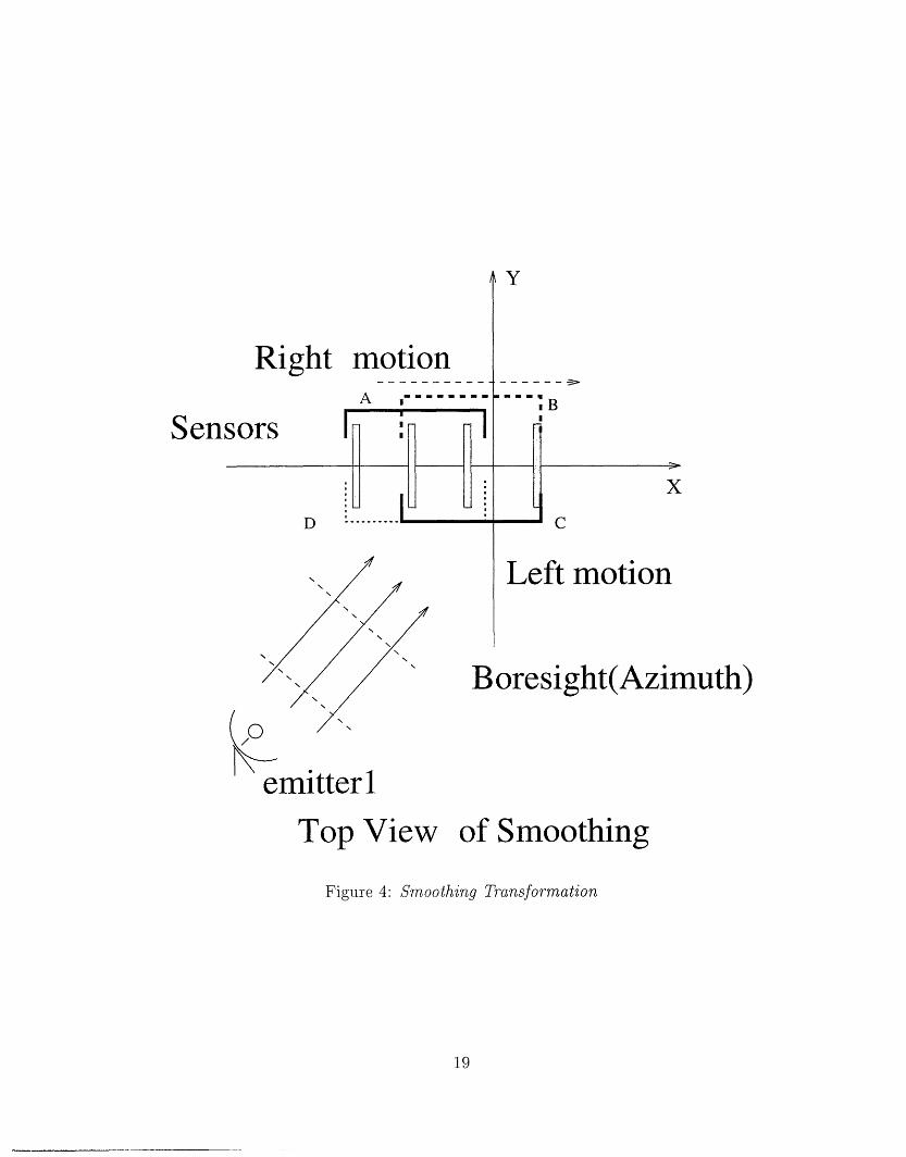
In a more general scenario where more than two coherent sources are present, forward-backward averaging cannot restore the rank of the signal covariance matrix on its own.A heuristic solution of this problem was first proposed in [128] for uniform linear arrays,and later formalized and extended8 in [31, 93]. The idea of the so-called spatial smoothingtechnique is to split the ULA into a number of overlapping subarrays. The steering vectorsof the subarrays are assumed to be identical up to different scalings, and the subarrayoutputs can therefore be averaged before computing the covariance matrix. Similar to(41), the spatial smoothing induces a random phase modulation which in turn decorrelatesthe signals that caused the rank deficiency. This is pictorially shown in Figure 4.

Formally, the transformation can also be carried out by an averaging procedure ofoverlapping diagonal submatrices of the original covariance matrix R, and thus as aresult, "unfold" the collapsed signal subspace with an appropriate choice of the submatrixsize (i.e. subarray size). A compact expression for this smoothed matrix R can bewritten in terms of a filtering matrix F as follows. If p is a positive integer smallerthan L (p is the number of elements in the subarrays), n, = L-p + 1 is the number ofsubarrays, F = [F1plF2pl ... IFp], is a p x nsL windowing matrix defined by Fip =[Opx(i-1) IplOpx(L-i-p+l)], i = 1, 2,.. , ns, then we can write

R = F (Ins 0 (R)) FT

Here, 0 denotes the Kronecker matrix product and Ins is the ns x ns identity matrix. Therank of the averaged source covariance matrix P can be shown to increase by 1 w.p.1 [27]for each additional subarray in the averaging, until it reaches its maximum value M.

The drawback with spatial smoothing is that the effective aperture of the array is re-duced, since the subarrays are smaller than the original array. However, despite this loss

sThe so-called spatial smoothing transformation requires a translational invariance which is valid forULA. Conceptually, however, one could always map the steering vectors for any array into those of aULA and proceed with the transformation described here, see further [40].

17

of aperture, the spatial smoothing transformation mitigates the limitation of all subspace-based estimation techniques while retaining the computational efficiency of the unidimen-sional spectral searches. As seen in the next section, the parametric techniques, in generaldo not experience such problems when faced with coherent signals. They require, on theother hand a more complicated multidimensional search. Let us again stress on the factthat spatial smoothing and FB averaging is essentially limited to ULAs. When using moregeneral arrays (e.g. circular), some sort of transformation of the received data to that of aULA must precede the smoothing transformation. Such a transformation is conceptuallypossible, but requires in general some a priori knowledge of the source locations.

18

Y

Right motion

Sensors I l

xD ....... ' C

Left motion\

Boresight(Azimuth)

emitter 1

Top View of Smoothing

Figure 4: Smoothing Transformation

19

4 Parametric Methods

While the spectral-based methods presented in the previous section are computationallyattractive, they do not always yield sufficient accuracy. In particular, for scenarios in-volving highly correlated (or even coherent) signals, the performance of spectral-basedmethods may be insufficient. An alternative is to more fully exploit the underlying datamodel, leading to so-called parametric array processing methods. As we shall see, coher-ent signals impose no conceptual difficulties for such methods. The price to pay for thisincreased efficiency is that the algorithms typically require a numerical optimization tofind the estimates. For uniform linear arrays (ULAs), the search can, however, be avoidedwith little (if any) loss of performance.

Perhaps the most important model-based approach in signal processing is the maxi-mum likelihood (ML) technique. This methodology requires a statistical framework forthe data generation process. Though not necessary, the vast majority of existing MLalgorithms assume Gaussian noise. Two different assumptions about the emitter signalshave led to two different ML approaches in the array processing literature. The signalsare either regarded as arbitrary unknown sequences, or they are modeled as Gaussianrandom processes similar to the noise. These two signal models result in the determin-istic (or conditional) and the stochastic (or unconditional) ML methods respectively. Inthis section, we will briefly review both of these approaches, discuss their relative merits,and present two subspace-based ML approximations. Parametric DOA estimation meth-ods are in general computationally quite complex. However, for ULAs a number of lessdemanding algorithms are known, as presented in Section 4.4.

4.1 Deterministic Maximum Likelihood

While the background and receiver noise in the assumed data model, can be thoughtof as emanating from a large number of independent noise sources, the same is usuallynot the case for the emitter signals. It therefore appears natural to model the noise as astationary Gaussian white random process whereas the signal waveforms are deterministic(arbitrary) and unknown. Assuming spatially white and circularly symmetric 9 noise, thesecond-order moments of the noise term take the form

E{n(t)nH(s)} = 2 I 5t,s (42)

E{n(t)nT (s)} = 0. (43)

As a consequence of the statistical assumptions, the observation vector x(t) is also acircularly symmetric and temporally white Gaussian random process, with mean A(O)s(t)and covariance matrix r 2 I. The likelihood function is the probability density function(PDF) of all observations given the unknown parameters. The PDF of one measurement

9A complex random process is circularly symmetric if its real and imaginary parts areidentically distributed and have a skew-symmetric cross-covariance, i.e., E[Re(n(t))Im(n T(t))]-E[Im(n(t))Re(n T (t))].

20

vector x(t) is the complex L-variate Gaussian:

1 eJ1x(t)-As(t)ll2/2 (44)

where . [ denotes the determinant, 11 11 the Euclidean norm, and the argument of A(0)has been dropped for notational convenience. Since the measurements are independent,the likelihood function is obtained as

LDML(O, S(t), ur2) = UtN 1((T2)- L elI x(t) - As(t)ll 2 /a2 (45)

As indicated above, the unknown parameters in the likelihood function are the signalparameters 0, the signal waveforms s(t) and the noise variance cr2 . The ML estimates ofthese unknowns are calculated as the maximizing arguments of L(O, s(t), u 2 ), the rationalebeeing that these values make the observations as probable as possible. For convenience,the ML estimates are alternatively defined as the minimizing arguments of the negativelog-likelihood function - log L(O, s(t), o2 ). Normalizing by N and ignoring the parameter-independent L log 7r-term, we get

1 NIDML(O, s(t), 7

2) = LlogU +2 N 1S E X(t) - As(t)1 2 (46)t=l

whose minimizing arguments are the deterministic maximum likelihood (DML) estimates.As shown in [14, 122], explicit minima with respect to U2 and s(t) can be obtained as

2 Tr{qlft} (47)

s(t) = Atx(t), (48)

where R is the sample covariance matrix, At is the Moore-Penrose pseudo-inverse of Aand HI i is the orthogonal projector onto the nullspace of AH, i.e.

N

-= y Ex(t)xH (t) (49)t=l

At = (AHA)-1AH (50)

HA = AAt (51)

IA =: I-I A. (52)

Substituting (47)-(48) into (45) shows that the DML signal parameter estimates areobtained by solving the following minimization problem:

oDML = arg {min Tr{II R}} (53)

21

The interpretation is that the measurements x(t) are projected onto a model subspaceorthogonal to all anticipated signal components, and a power measurement

N t=l IzIHIx(t) = Tr{IIAR} is evaluated. The energy should clearly be smallest whenthe projector indeed removes all the true signal components, i.e., when 0 = 00. Since onlya finite number of noisy samples is available, the energy is not perfectly measured andODML will deviate from 00. However, if the scenario is stationary, the error will convergeto zero as the number of samples is increased to infinity . This remains valid for correlatedor even coherent signals, although the accuracy in finite samples is somewhat dependentupon signals correlations.

To calculate the DML estimates, the non-linear M-dimensional optimization problem(46) must be solved numerically. Finding the signal waveform and noise variance estimates(if desired) is then straightforward, by inserting 0 DML into (47)-(48). Given a good initialguess, a Gauss-Newton technique (see e.g. [22, 118]) usually converges rapidly to theminimum of (46). Obtaining sufficiently accurate initial estimates, however, is generally acomputationally expensive task. If these are poor, the search procedure may converge toa local minimum, and never reach the desired global minimum. A spectral-based method(see Section 3) is a natural choice for an initial estimator, provided all sources can beresolved. Another possibility is to apply the alternating projection technique of [141].However, convergence to the global minimum can still not be guaranteed. Some moreaspects on the global properties of the criteria can be found in [77].

4.2 Stochastic Maximum Likelihood

The other ML technique reported in the literature is termed the stochastic maximumlikelihood (SML) method. This method is obtained by modeling the signal waveforms asGaussian random processes. This model is reasonable, for instance, if the measurementsare obtained by filtering wideband signals using a narrow bandpass filter data. It is, how-ever, important to point out that the method is applicable even if the data is not Gaussian.In fact, the asymptotic (for large samples) accuracy of the signal parameter estimates canbe shown to depend only on the second-order properties (powers and correlations) of thesignal waveforms [100, 76]. With this in mind, the Gaussian signal assumption is merelya way to obtain a tractable ML method. Let the signal waveforms be zero-mean withsecond-order properties

E{s(t)sH(s)} = PSt,s (54)E{s(t)sT (s)} = 0. (55)

Then, the observation vector x(t) is a white, zero-mean and circularly symmetric Gaussianrandom vector with covariance matrix

R = A(0)PAH(0) + .2I . (56)

The set of unknown parameters is in this case, different from that in the deterministicsignal model. Now, the likelihood function depends on 0, P and a2. The negative log-

22

likelihood function (ignoring constant terms) is in this case easily shown to be

ISML(0, P, 2)= log JRI + Tr{R-1 R} . (57)

Though this is a highly non-linear function, this criterion allows explicit separation ofsome of the parameters. For fixed 0, the minimum with respect to u2 and P can beshown to be (although this requires some tedious calculations [15, 51])

cSML(O) L-M Tr{A (58)

PSML(O) = At(R - 2SML(0) I)AtH (59)

When (58)-(59) are substituted into (57), the following compact form of the criterion isobtained

obt dSML = arg {min log APSML(O)AH +&ML()I} (60)

In addition this criterion has a nice interpretation, namely that the determinantAPSML(0)AH + 82ML() I , termed the generalized variance in the literature, measures

the volume of a confidence interval for the data vector. Note that the argument of thedeterminant is the structured ML estimate of the array covariance matrix! Consequently,we are looking for the model occupying the least volume, to obtain the "cheapest possible"explanation of the data.

The criterion function in (60) is also a higly non-linear function of its argument 0. ANewton-type technique implemention of the numerical search is reported in [77] and anexcellent statistical accuracy results when the global minimum is attained. Indeed, theSML signal parameter estimates have been shown to have a better large sample accuracythan the corresponding DML estimates [100, 76], with the difference being significantonly for small numbers of sensors, low SNR and highly correlated signals. This is trueregardless of the actual distribution of the signal waveforms, in particular they need not beGaussian. For Gaussian signals, the SML estimates attain the Cramer-Rao lower bound(CRB) on the estimation error variance, derived under the stochastic signal model. Thisfollows from the general theory of ML estimation (see e.g. [112]), since all unknowns in thestochastic model are estimated consistently. The situation is different in the deterministicmodel for which the number of signal waveform parameters s(t) grows without boundas the number of samples -increases: they cannot be consistently estimated. Hence, thegeneral ML theory does not apply and the DML estimates do not attain the corresponding("deterministic") CRB.

4.3 Subspace-Based Approximations

As noted in Section 3, subspace-based methods offer significant performance improve-ments in comparison to conventional beamforming methods. In fact, the MUSIC methodhas been shown to yield estimates with a large-sample accuracy identical to that of theDML method, provided the emitter signals are uncorrelated [97]. The spectral-based

23

methods, however, usually suffer from a large bias in finite samples, leading to resolutionproblems. This problem is accentuated for increasing source correlation. Recently, para-metric subspace-based methods that practically have the same statistical performance asthe ML methods have been developed [101, 102, 117, 118]. The computational cost forthese so-called Subspace Fitting methods is, however, less than for the ML dito. As willbe seen in Section 4.4.3, a computationally attractive implementation is known for theubiquitous case of a uniform linear array.

Recall the structure of the eigendecomposition of the array covariance matrix (32),

R = APAaH +r 2 I (61)

= U:AU + U2 U7U+ (62)

As previously noted, the matrices A and Us span the same range space whenever P hasfull rank. In the general case, the number of signal eigenvectors in Us equals M', therank of P. The matrix Us will then span an M'-dimensional subspace of A. To see this,express the identity in (61) as I = U'sU + UU/. Cancelling the o2 UnU[-term thenyields

APAH + o 2 UUH = UsASUf . (63)

Post-multiplying on the right by Us (note that U'HU, = I) and re-arranging gives therelation

Us = AT, (64)

where T is the full-rank M x M' matrix

T = PAHU,(As -_ 2 I) - 1 (65)

The relation (64) forms the basis for the Signal Subspace Fitting (SSF) approach. Since0 and T are unknown, it appears natural to search for the values that solve (64). Theresulting 0 will be the true DOAs (under general identifiability conditions [126]), whereasT is an uninteresting "nuisance parameter". When only an estimate Us of Us is available,there will be no such solution. Instead, we try to minimize some distance measure betwenUs and AT. The Frobenius norm, defined as the square-root of the sum of squaredmoduli of the elements of a matrix, is a useful measure for this purpose. Alternatively,the squared Frobenius norm can be expressed as the sum of the squared Euclidean normsof the rows or columns. The connection to standard least-squares estimators is thereforeclear. The SSF estimate is obtained by solving the following non-linear optimizationproblem:

{S T} = arg min lus - ATF . (66)O,T

Similar to the DML criterion (46), this is a separable non-linear least squares problem[44]. The solution for the linear parameter T (for fixed unknown A) is

i = AtUs. (67)

24

Substituting (67) into (66) leads to the separated criterion function

0 = arg {min Tr{Ij,,UsAsU }}. (68)

Since the eigenvectors are estimated with different quality, depending on how close thecorresponding eigenvalues are to the noise variance, it is natural to introduce a weightingof the eigenvectors. We thus arrive at the form

bSSF = arg {minTr{iAUsWU'}} . (69)

A natural question is how to pick W to maximize the accuracy, i.e., to minimize theestimation error variance. It can be shown that the projected eigenvectors IIA(00o)ik, k -1,.. ., ,M' are asymptotically independent. Hence, following from the theory of weightedleast squares, [43], W should be a diagonal matrix containing the inverse of the covariancematrix of H(00o)fk, k = 1,... , M'. This leads to the choice [102, 117]

Wt = (A, - -2 I) 2A (70)

Since Wopt depends on unknown quantities, we use instead

W opt- (& - .2 I)2A~' 1 , (71)

where &2 denotes a consistent estimate of the noise variance, for example the averageof the L - M' smallest eigenvalues. The estimator defined by (69) with weights givenby (71) is termed the Weighted Subspace Fitting (WSF) method. It has been shown totheoretically yield the same large sample accuracy as the SML method, and at a lowercomputational cost provided a fast method for computing the eigendecomposition is used(see Section 5.5). Practical evidence, see e.g. [77], have given by hand that the WSF andSML methods also exhibit similar small sample (i.e. threshold) behaviour.

An alternative subspace fitting formulation is obtained by instead starting from the"MUSIC relation"

AH(0)U, = 0 iff 0 = 0 , (72)

which holds for P having full rank. Given an estimate of U,, it is natural to look for thesignal parameters that minimize the following Noise Subspace Fitting (NSF) criterion,

0 = arg{minTr{A HUnU AV} , (73)

where V is some positive (semi-)definite weighting matrix. Interestingly enough, theestimates calculated by (73) and (69) asymptotically coincide, if the weighting matricesare (asymptotically) related by [77]

V = At(0O)UsWUf'At*(0o) . (74)

25

Note also that the NSF method reduces to the MUSIC algorithm for V = I, providedla(O)l is independent of 0. Thus, in a sense the general estimator in (73) unifies theparametric methods and also encompasses the spectral-based subspace methods.

The NSF method has the advantage that the criterion function in (73) is a quadraticfunction of the steering matrix A. This is useful if any of the parameters of A enterlinearly. An analytical solution with respect to these parameters is then readily available(see e.g. [119]). However, this happens only in very special situations, rendering thisforementioned advantage of limited importance. The NSF formulation is also fraught withsome drawbacks, namely that it cannot produce reliable estimates for coherent signals,and that the optimal weighting Vopt depends on 00, so that a two-step procedure has tobe adopted.

4.4 Uniform Linear Arrays

The steering matrix for a uniform linear array has a very special, and as it turns out,useful structure, which, as described next, will result in enhanced performance. From(28), the ULA steering matrix takes the form

1 I ... 1 ejol eJh2 ... ejiM

A(0)= : : : (75)

ej(L-1)0i ej(L-1)02 ... ej(L-1)qkm

This structure is referred to as a Vandermonde matrix [44].

4.4.1 Root-MUSIC

The Root-MUSIC method [11], as the name implies, is a polynomial-rooting version ofthe orginal MUSIC technique. The idea dates back to Pisarenko's method [81]. The basicobservation is that the polynomial

pk(z)= uHa(z) k - M + 1, + 2,.. .,L, (76)

wherea(z) [1, z,..., ZL- 1], (77)

has M of its zeros at ej l , I 1, 2, . . , M provided that P has full rank. To exploit theinformation from all noise eigenvectors simultaneously, we want to find the zeros of theMUSIC function

lUn a(z)112 = aH ( z ) U n Un a(z). (78)

However, the latter function is not a polynomial in z, which complicates the search forzeros. Since we are interested in values of z on the unit circle, we can use aT(z- 1) foraH(z), which gives the Root-MUSIC polynomial

P(Z) zL aT(z-1)U Un a(z)a(z)a (79)

26

Note that P(z) will have M roots inside the unit circle (UC), that have M mirroredimages outside the UC. Of the ones inside, the phases of the M closest to the UC, say21, Z2 ,. . , ZM, yield the DOA estimates, as

k =- arcsin ( d arg(zk)) (80)

It has been shown [97, 98] that MUSIC and Root-MUSIC have identical asymptoticproperties, although in small samples Root-MUSIC has empirically been found to performsignificantly better. As previously alluded to, this can be attributed to a larger bias forspectral-based methods, as compared to the parametric techniques [62, 85].

4.4.2 ESPRIT

The ESPRIT algorithm [80, 87] uses the structure of the ULA steering vectors in a slightlydifferent way. The observation here is that A has a so-called shift structure. Define thesub-matrices Al and A 2 by deleting the first and last rows from A respectively, i.e.

A [ ,, Al i [ first row (81)A last row A2

By the structure (75), A1 and A 2 are related by the formula

A2 - Al 4X, (82)

where D is a diagonal matrix having the "roots" ej0k, k = 1, 2, . . ., M on the diagonal.Thus, the DOA estimation problem can be reduced to that of finding -(. Like the othersubspace-based algorithms, ESPRIT relies on properties of the eigendecomposition of thearray covariance matrix. Recall the relation (64). Deleting the first and last rows of (64)respectively, we get

U 1 = A 1T , U 2 = A 2T, (83)

where U, has been partitioned conformably with A into the sub-matrices U1 and U 2.Combining (82) and (83) yields

U 2 = AjlT = U 1T-14T . (84)

Finally, defining 'I, = T-1 4T we obtain

U 2 = U1 . (85)

Note that I and '1 are related by a similarity transformation, and hence have the sameeigenvalues. The latter are of course given by ejik, k = 1, 2,.. ., M, and are related tothe DOAs by (80). The ESPRIT algorithm is now stated:

1. Compute the eigendecomposition of the array covariance matrix

2. Form U1 and U2 from the M principal eigenvectors

27

3. Solve the approximate relation (85) in either a Least-Squares sense (LS-ESPRIT)or a Total-Least-Squares [43, 44] sense (TLS-ESPRIT)

4. The DOA estimates are obtained by applying the inversion formula (80) to theeigenvalues of 4i

It has been shown that LS-ESPRIT and TLS-ESPRIT yield identical asymptotic estima-tion accuracy [84], although in small samples TLS-ESPRIT usually has an edge.

4.4.3 IQML and Root-WSF

Another interesting exploitation of the ULA structure was presented in [17], although theidea can be traced back to the Steiglitz and McBride algorithm for system identification[96]. The IQML algorithm is an iterative procedure for minimizing the DML criterion

V(O) = Tr{IIIA } (86)

The idea is to re-parametrize the projection matrix HIA using a basis for the nullspaceof AH. Towards this end, define the polynomial b(z) to have its M roots at ejok, k1, 2,..., M, i.e.,

b(z) = z + blzM- +. + bM = nk= (Z -eik) (87)

Then, by construction the following relation holds true

bm bM- ... I °| 1 j .. 1 1

[O b. 1-1 *eJ1 b.. (88)0 bMi bM- ... ej(Ll)01 ... ej(L-1lx.m

BHA = 0.

Since B has full rank L - M, its columns do in fact form a basis for the nullspace of AH.Apparently the orthogonal projections onto these subspaces must coincide, implying

I[- = B(BHB)-lBH (89)

Now the DML criterion function can be parametrized by the polynomial coefficients bk inlieu of the DOAs Ok. The DML estimate (53) can be calculated by solving

b = arg min Tr{B(BHB)-1BHR} (90)b

and then applying (80) to the roots of the estimated polynomial. Unfortunately, (90)is still a difficult non-linear optimization problem. However, [17] suggested an iterativesolution as follows

1. Set U= I

28

2. Solve the quadratic problem

b = arg min Tr{BUBHR} (91)

3. Form 1B and put U = (BHB3)-1

4. Check for convergence. If not, goto Step 2

5. Apply (80) to the roots of b(z).

Since the roots of b(z) should be on the UC, [18] suggested using the constraint

bk = bH_k, k = 1,2,...,M (92)

when solving (91). Now, (92) does not guarantee roots on the UC, but it can be shownthat the accuracy loss due to this fact is negligible. While the above described IQML(Iterative Quadratic Maximum Likelihood) algorithm cannot be guaranteed to converge,it has indeed been found to perform well in simulations.

An improvement over IQML was introduced in [101]. The idea is simply to apply theIQML iterations to the WSF criterion (69). Since the criteria have the same form, themodification is straightforward. However, there is a very important advantage of usingthe rank-truncated form UTWUI' rather than R in (91). That is, after the second passof the iterative scheme, the estimates already have the asymptotic accuracy of the trueoptimum! Hence, the resulting IQ-WSF algorithm is no longer an iterative procedure:

1. Solve the quadratic problem

b = arg min Tr{BBHUTWU(Y } (93)

2. Solve the quadratic problem

1 = arg min Tr{B(B3H i)-1BHUsWUsH} (94)

3. Apply (80) to the roots of b(z).

Note that this algorithm is essentially in closed form (if one accepts solving for the eigen-decomposition and polynomial rooting as closed form), and that the resulting estimateshave the best possible asymptotic accuracy. Thus, the IQ-WSF algorithm is a strongcandidate for the "best" method for ULAs.

29

5 Additional Topics

The emphasis in this paper is on computational methods for sensor array processing.Because of space limitations, we have omitted several interesting topics from the maindiscussion and instead give a very brief overview of these additional topics in this section.We structure this section in the form of a commented enumeration of references to selectedspecialized papers.

5.1 Number of Signals Estimation

In applications of model-based methods, an important problem is the determination ofM, the number of signals. In the case of non-coherent signals, the number of signalsis equal to the number of "large" eigenvalues of the array covariance matrix. This factis used to obtain relatively simple non-parametric algorithms for determining M. Themost frequently used approach emanates from the factor analysis literature [4]. The ideais to determine the multiplicity of the smallest eigenvalue, which theoretically equalsL - M. A statistical hypothesis test is proposed in [91], whereas [124, 140] are based oninformation theoretic criteria, such as Akaike's AIC (an information theoretic criterion)and Rissanen's MDL (minimum description length). Unfortunately, the above mentionedapproach is very sensitive to the assumption of a spatially white noise field [136]. Analternative idea based on using the eigenvectors rather than the eigenvalues is pursued inthe referenced paper. Another non-parametric method is presented in [29].

In the presence of coherent signals, the above mentioned methods will fail as stated,since the dimension of the signal subspace then is smaller than M. However, for ULAs onecan test the eigenvalues of the spatially smoothed array covariance matrix to determineM [93], with further improved performance in [61].

A more systematic approach to estimating the number of signals is possible if themaximum likelihood estimator is employed. A classical generalized likelihood ratio test(GLRT) is described in [77], whereas [123] presents an information theoretic approach.Another model-based detection technique is presented in [118, 77], based on the weightedsubspace fitting method. The model-based methods for determining the number of signalsrequire calculating signal parameter estimates for an increasing hyphotesized numbers ofsignals, until some pre-specified criterion is met. Hence, the approach is inherently morecomputationally complex than the non-parametric tests. Its performance in difficult signalscenarios is, however, improved and the model-based technique is less sensitive to smallperturbations of the assumed noise covariance matrix.

5.2 Reduced Dimension Beamspace Processing

Except for the beamforming-based methods, the estimation techniques discussed hereinrequire that the outputs of all elements of the sensor array be available in digital form.In many applications, the required number of high-precision receiver front-ends and A/Dconverters may be prohibitive. Arrays of 104 elements are not uncommon, for example in

30

radar applications. Techniques for reducing the dimensionality of the observation vectorwith minimal effect on performance, is therefore of great interest. As already discussedin Section 3.2.3, a useful idea is to employ a linear transformation

z(t) = T*x(t),

where T is L x R, with (usually) R < L. The transformation is typically implemented inanalog hardware, thus significantly reducing the number of required A/D converters. Thereduced-dimension observation vector z(t) is usually referred to as the beamspace data,and T is a beamspace transformation.

Naturally, processing the beamspace data significantly reduces the computational loadof the digital processor. However, reducing the dimension of the data also implies a lossof information. The beamspace transformation can be thought of as a multichannelbeamformer. By designing the beamformers (the columns of T) so that they focus on arelatively narrow DOA sector, the essential information in x(t) regarding sources in thatsector can be retained in z(t). See e.g., [38, 116, 138, 142] and the references therein. Withfurther a priori information on the locations of sources, the beamspace transformationcan in fact be performed without losing any information at all [5]. As previously alludedto, beamspace processing can even improve the resolution (the bias) of spectral-basedmethods.

Note that the beamspace transformation effectively changes the array propagationvectors from a(O) into T*a(O). It is possible to utilize this freedom to give the beamspacearray manifold a simpler form, such as that of a ULA, [40]. Hence, the computationallyefficient ULA techniques (see Section 3 are applicable in beamspace. In [71], a transfor-mation that maps a uniform circlar array into a ULA is proposed and analyzed, enablingcomputationally efficient estimation of both azimuth and elevation.

5.3 Estimation Under Model Uncertainty

As implied by the terminology, model-based signal processing relies on the availability ofa precise mathematical description of the measured data. When the model fails to reflectthe physical phenomena with a sufficient accuracy, the performance of the methods will ofcourse degrade. In particular, deviations from the assumed model will introduce bias inthe estimates, which for spectral-based methods is manifested by a loss of resolving powerand a presence of spurious peaks. In principle, the various sources of modeling errors canbe classified into noise covariance and array response perturbations.

In many applications of interest, such as communication, sonar and radar, the back-ground noise is dominated by man-made noise. While the noise generated in the receivingequipment is likely to fulfill the spatially white assumption, the man-made noise tends tobe quite directional. The performance degradation under noise modeling errors is studiedin, e.g. [68, 121]. One could in principle envision extending the model-based estimationtechniques to also include estimation of the noise covariance matrix. Such an approach hasthe potential of improving the robustness to errors in the assumed noise model [131, 123].However, for low SNR's, this solution is less than adequate. The simultaneous estimation

31

of a completely unknown noise covariance matrix and of the signal parameters poses aproblem unless some additional information which enables us to separate signal from noise,is available. It is, for example, always possible to infer that the received data is nothingbut noise, and that the (unknown) noise covariance matrix is precisely the observed arraysample covariance matrix. Estimation of a parametric (structured) noise models is con-sidered in, e.g. [16, 57]. So-called instrumental variable techniques are proposed, e.g. in[104] (based on assumptions on the temporal correlation of signals and noise) and [132](utilizing assumptions on the spatial correlation of the signals and noise). Methods basedon other assumptions appeared in [79, 114].

At high SNR, the modeling errors are usually dominated by errors in the assumed sig-nal model. The signals have a non-zero bandwidth, the sensor positions may be uncertain,the receiving equipment may not be perfectly calibrated, etc. The effects of such errorsis studied e.g. in [39, 67, 108, 109]. In some cases it is possible to physically quantify theerror sources. A "self-calibrating" approach may then be applicable [86, 127, 119], albeitat a quite a computational cost. In [108, 109, 120], robust techniques for unstructuredsensor modeling errors are considered.

5.4 Wideband Data Processing

The methods presented herein are essentially limited to processing narrowband1 0 data.In many applications (e.g. radar and communication), this is indeed a realistic assump-tion. However, in other cases (e.g. sonar), the received signal may be broadband. Anatural extension of methods for narrowband data is to employ narrowband filtering, forexample using the Fast Fourier Transform (FFT). An optimal exploitation of the dataentails combining information from different frequency bins [59], see also [125]. A simplersuboptimal approach is to process the different FFT channels separately using a standardnarrowband method, whereafter the DOA estimates at different bins must be somehowcombined.

Another approach is to explicitly model the array output as a multidimensional timeseries, using an auto-regressive moving average (ARMA) model. The poles of the systemare estimated, e.g. using the overdetermined Yule-Walker equations. A narrowbandtechnique can subsequently be employed using the estimated spectral density matrix,evaluated at the system poles. In [106], the MUSIC algorithm is applied, whereas [75]proposes to use the ESPRIT algorithm.

A wideband DOA estimation approach inspired by beamspace processing is the so-called coherently averaged signal subspace method. The idea is to first estimate thesignal subspace at a number of FFT channels. Then, the information from differentfrequency bins is merged by employing linear transformations. The objective is to makethe transformed steering matrices A at different frequencies as identical as possible, forexample by focusing at the center frequency of the signals. See, e.g. [50, 94] for furtherdetails.

10Signals whose bandwidths are much smaller than the inverse of the time it takes a wavefront topropagate across the array, are referred to as narrowband.

32

5.5 Fast Subspace Calculation and Tracking

When implementing subspace-based methods in applications with real-time operation,the bottleneck is usually the calculation of the signal subspace. A scheme for fast compu-tation of the signal subspace is proposed in [54], and methods for subspace tracking areconsidered in [28]. The idea is to exploit the "low-rank plus a 2 I" structure of the idealarray covariance matrix. An alternative gradient-based technique for subspace tracking isproposed in [139]. Therein, it is observed that the solution of the constrained optimizationproblem, W,

max Tr{W*RW}w

subject to W*W = I

spans the signal subspace.For some methods, estimates of the individual principal eigenvectors are required, in

addition to the subspace they span. A number of different methods for eigenvalue/vector1ltracking is given in [26]. A more recent approach based on exploiting the structure of theideal covariance is proposed and analyzed in [134]. The so-called fast subspace decomposi-tion (FSD) technique is based on a Lanczos method for calculating the eigendecoposition.It is observed that the Lanczos iterations can be prematurely terminated without anysignificant performance loss.

5.6 Signal Structure Methods

Most "standard" approaches to array signal processing make no use of any available in-formation of the signal structure. However, many man-made signals have a rich structurethat can be used to improve the estimator performance. In digital communication ap-plications, the transmitted signals are often cyclostationary, i.e. their autocorrelationfunctions are periodic. This extra information is exploited in e.g. [1, 133, 90], and algo-rithms for DOA estimation of cyclostationary signals are derived and analyzed. In thisapproach, the wideband signals are easily incorporated into the framework, and there canbe more signals than sensors, provided not all of them share the same cyclic frequency.

A different approach utilizing signal structure is based on high-order statistics. As iswell-known, all information about a Gaussian signal is conveyed in the first and secondorder moments. However, for non-Gaussian signals, there is potentially more to be gainedby using higher moments. This is particularly so if the noise can be regarded as Gaus-sian. Then, the high-order cumulants will be noise-free, because they vanish for Gaussiansignals. Methods based on the fourth-order cumulant are proposed in [82, 24], whereas[92] proposes to use high-order cyclic spectra (for cyclostationary signals).

A common criticism to both methods based on cyclostationarity and those based onhigh-order statistics is that they require a considerable amount of data to yield reliable

1 1The referenced paper considers tracking of the principal left singular values of the data matrix. Math-ematically, but perhaps not numerically, these are identical to the eigenvectors of the sample covariancematrix.

33

results. This is because the estimated cyclic and high-order moments typically convergemore slowly towards their theoretical values as the number of data is increased.

5.7 Time Series Analysis

The DOA estimation problem employing a ULA has strong similarities with time seriesanalysis. Indeed, an important pre-cursor of the MUSIC algorithm is Pisarenko's method[81] for estimation of the frequencies of damped/undamped sinuoids in noise, when givenmeasurements of their covariance function. Likewise, Kung's algorithm for state-spacerealization of a measured impulse response [65] is an early version of the ESPRIT algo-rithm. An important difference between the time series case and the (standard) DOAestimation problem is that the time series data is usually estimated using a sliding win-dow. A "sensor array-like data vector" x(t) is formed from the scalar time series y(t) byusing

x(t) = [y(t),y(t + 1),...,y(t + L - 1)]T

The windowing transformation induces a temporal correlation in the L-dimensional timeseries x(t), even if the scalar process y(t) is temporally white. This fact complicates theanalysis, as in the case of spatial smoothing in DOA estimation, see e.g. [25, 103, 61].

34

6 Applications

The research progress of parameter estimation and detection in array processing hasresulted in a great diversity of applications, and continues to provide fertile ground fornew ones. In this section we discuss three important application areas, and in additiondemonstrate the performance of the algorithms on a real data example.

6.1 Personal Communications

Receiving arrays and related estimation/detection techniques have long been used in HighFrequency communications. These applications have recently reemerged and receiveda significant attention by researchers, as a potentially useful "panacea" for numerousproblems in personal communications (see e.g. [130, 107, 3, 105]). They are expectedto play a key role in accomodating a multiuser communication environment, subject tosevere multipath.

One of the most important problems in a multiuser asynchronous environment isthe inter-user interference, which can degrade the performance quite severely. This isthe case also in a practical Code-Division Multiple Access (CDMA) system, because thevarying delays of different users induce non-orthogonal codes. The base stations in mobilecommunication systems have long been using spatial diversity for combatting fading dueto the severe multipath. However, using an antenna array of several elements introducesextra degrees of freedom, which can be used to obtain higher selectivity. An adaptivereceiving array can be steered in the direction of one user at a time, while simultaneouslynulling interference from other users, much in the the same way as the beamformingtechniques described in Section 3.

Figure 5 illustrates a personal communication scenario involving severe multipath.The multipath introduces difficulties for conventional adaptive array processing. Unde-sired cancellation may occur [128], and spatial smoothing may be required to achievea proper selectivity. In [3], it is proposed to identify all signal paths emanating fromeach user, whereafter an optimal combination is made. A configuration equivalent to thebeamspace array processing with a simple energy differencing scheme serves in localizingincoming users waveforms [89]. This beamspace strategy underlies an adaptive optimiza-tion technique proposed in [105], which addresses the problem of mitigating the effects ofdispersive time varying channels.

Communication signals have a rich structure that can be exploited for signal separationusing antenna arrays. Indeed, the DOAs need not be estimated. Instead, signal structuremethods such as the constant-modulus beamformer [45] have been proposed for directlyestimating the steering vectors of the signals, thereby allowing for blind (i.e., not requiringa training sequence) signal separation. Techniques based on combining beamformingand demodulation of digitally modulated signals have also recently been proposed (see[70, 110, 95, 111]). It is important to note that the various optimal and/or suboptimalproposed methods are of current research interest, and that in practice, many challengingand interesting problems remain to be addressed.

35

Reflexions due to Obastacles

Base Station Array

Mobile Communications Environment

Figure 5: Mobile Radio Scenario with an Adaptive Array

6.2 Radar and Sonar

Modern techniques in array processing have also found an extensive use for in radar andsonar [69, 78, 47, 32, 48]. The antenna array is, for example, used for source localization,interference cancellation and ground clutter suppression.

In radar applications, the mode of operation is referred to as active. This is on accountof the role of the antenna array based system which radiates pulses of electromagneticenergy and listens for the return. The parameter space of interest may vary according to

36

the geometry and sophistication of the antenna array. The radar returns enable estimationof parameters such as velocity, range, direction of arrival of targets of interest [112].More recently, researchers have focused on an extension of the spatial sampling conceptof an array to synthesize a highly resolving array with a moving airborn sensor whichperiodically transmits/receives electromagnetic energy. Such a synthetic aperture radar(SAR) system is pictorially shown in Figure 6.

J_ V

Range Resolution= c I u W ( Beam Width angle)

Point Targets

Cross-Range Resolution = X-------- -> 2V

Figure 6: Synthetic Aperture Radar System

The fraction of the scattered energy which is reflected towards the synthesized array,when appropriately processed, i.e. integrated over the range and cross-range (region along

37

the flight plan), and adequately deconvolved, result in the reflectivity of the background,thus permitting its imaging. Numerous important areas of applications in remote sensing,include environmental studies (forrestation etc.), meteorological predictions, oceanographyand many others.

Sonar applications, on the other hand, use acoustic energy and can operate in an activeas well as passive mode. In a passive mode, the receiving array is generally in a listeningmode to detect and process any acoustic energy emanating from sources. It thus has thecapability to locate distant sources. Deformable array models are often used in sonar,as the receiving antenna is typically towed under water [69]. Techniques with piecewiselinear subarrays are used in the construction of the overall solution.

In an active mode, a sonar system emits acoustic (electromagnetic arrays are also usedunderwater) energy and monitors and retrieves whatever echo. This again can be usedfor parameter estimation, such as bearings and velocity etc., using the delay of the echo.Despite its limitations due to the speed of sound, sonar together with related estimationtechniques, remains a reliable tool for range, bearing estimation and other imaging tasksin underwater applications. However, the difficult propagation conditions under watermay call for more advanced signal modeling, such as in matched field processing (see e.g.[10]).

6.3 Industrial applications

Sensor array signal processing techniques have drawn much interest from industrial ap-plications, such as manufacturing and medical applications. In medical imaging andhyperthermia treatment [35, 36], circular arrays are commonly used as a means to focusenergy in both an injection mode as well as reception mode. It has also been used in treat-ment of tumors [34]. In electrocardiograms, planar arrays are used to track the evolutionof wavefronts which in turn provide information about the condition of an individual'sheart. Array processing methods have also been adopted to localize brain activity usingbiomagnetic sensor arrays (SQUID sensors) [74]. It is expected that the medical appli-cations will proliferate as more resolution is sought, e.g. signals emanating from a wombmay be of more interest than those of a mother.

Other applications in industry are almost exclusively in automatic monitoring and faultdetection/localization. In engines, sensors are placed in a judicious and convenient way todetect and potentially localize faults such as knocks or broken gears [46]. One emergingand important application of array signal processing is in using notions from optics tocarry out tasks in product quality assurance in a manufacturing environement [2], and inobject shape characterization in tomography [72, 73]. An semiconductor manufactoringexample is provided in the following.

As noted earlier, it is often desired to minimize a human input in a manufacturingenvironment, for a number of reasons (e.g. cost, reliability, etc.). Sensor array processingapplications in such an environment have recently been reported. An array of photosensorsis used to monitor reflections from a surface, whose image is given in Figure 7. Thisimage could conceptually represent a number of products, but in this case it is that

38

of a semiconductor wafer which bears a scratch which, for obvious reasons needs to bedetected and its position estimated. In Figures 8 and 9, the ESPRIT method is used toestimate the parameters of the diagonal line, namely the coordinates (pixel offset fromthe left upper corner) as well as the angle of inclination with respect to the vertical. Inthese Figures, the parametric solution is compared to a more conventional non-parametricmethod that is more well-known in the area of tomography - the Hough transform. TheESPRIT method performs at least as good as the Hough transform, and on account ofits simple implementation, ESPRIT is a promising technique for such applications. Notethat the Hough transform requires a great deal of data which in turn is memory intensive,while the computational as well as the storage requirements with ESPRIT is much moreadvantageous.

39

Figure 7: Semiconductor chip with an inscribed line

40

1 1.2 1.4 1.6 1.8 2 2.2 2.4 2.6 2.8 3

Angle (degrees)

Figure 8: Line angle estimate using the ESPRIT (dashed vertical line) and the HoughTransform (solid line) methods.

41

0.9

0.8

0.7

0.6

0.5

0.4

0.3

0.2

0.1

020 30 40 50 60 70 80

Offset (pixels)

Figure 9: Line offset estimate using the ESPRIT (dashed vertical line) and the HoughTransform (solid line) methods.

42

7 Real Data Example

In this section, the viability of the various methods is tested on experimental radar data,provided by Professor S. Haykin of McMaster University. The receiver is an L = 32-element uniform linear array, which is mounted vertically so that the DOA is in this casethe elevation angle. The sensors have a horizontal polarization. The array is located onthe shore of a lake, whereas the transmitter is on the other side. Thus, the surface of thelake will ideally generate a specular multipath component. The orientation of the arrayis such that the direct and reflected waves impinge approximately symmetrically withrespect to the broadside. Five data sets have been processed, in which the separationbetween the two signal paths (in electrical angles, see (28)) varies between AO = BW/5and AO = BW/3, where BW = 27r/L represents the standard beamwidth of the array(in radians).

The given five data sets were processed using the previously presented methods as-suming a perfect ULA array response (28). In two of these data sets, none of the testedmethods was able to locate two signal components in the vicinity of the postulated truevalues. In the other three sets, fairly good results were obtained. The results from twoof the latter data sets are presented below. There are many possible reasons for the ob-served variability in the data. The most obvious is of course uncertainties in the receivingequipment, for example due to mutual coupling between sensor elements. The calibrationrequirements are generally quite high if one wants to achieve a resolution well within thebeamwidth of the array. Other possible sources of errors are insufficient signal-to-noiseratio (SNR), spatial correlation of the noise field, etc. To illustrate the latter point, theeigenvalues of a typical sample covariance are depicted in Figure 10, along with a real-ization from the theoretical model. One should also bear in mind that in a real dataexperiment, there are actually no true values available for the estimated parameters. Thepostulated AO is calculated from the geometry of the experimental setup, but in practicethe multipath component may very well be absent from some of the data sets, or it mayimpinge from an unexpected direction. In the following, the results from two successfuldata sets are presented. The sets are labeled A and B for reference. To obtain an ideaof the statistical variability of the estimates, the data sets, each containing N = 127snapshots, are first divided into 4 subsets of 32 samples (the last two subsets overlapby one snapshot). As a first attempt, the various spectral-based methods are applied.Since the signal components are expected to be highly correlated or even coherent, thespectral-based methods are likely to fail. However, the signals can be "de-correlated"by pre-processing the sample covariance matrix using forward-backward averaging (41).This has little or no effect on the beamforming techniques, but will be seen to improve theperformance of the spectral-based subspace methods, particularly so for the Min-Normmethod.

In Figure 11, the results from applying the traditional beamforming and the Caponmethods to the 4 different A subsets are presented. The "spatial spectra" are all nor-malized such that the peak value is unity. The "true" DOAs (electrical angles, measuredin fractions of the beamwidth) are indicated by vertical dotted lines in the plot. It is

43

Eigenvalue distribution10

10 5

Simulated data: o

10 - Real data set A: x

103

X X X

X X10 i_ 2 x X °°'°°0 0°00

X

105 10 15 20 25 30

Figure 10: Distribution of eigenvalues for 32-element uniform linear array. Simulateddata and real data set A.

clear that the beamforming methods fail to resolve the sources in this case. In Figure12, the results for the MUSIC method with and without forward-backward averaging areshown. The presence of the two signal components is visible for the FB-MUSIC method,but the resolution capability is still not quite adequate. Finally, the Min-Norm methodis applied and the resulting normalized "spatial spectra" are depicted in Figure 13. TheMin-Norm method is known to have better resolution properties than MUSIC because ofthe inherent bias in the radii of the roots [55, 62], and using forward-backward averagingwe see that Min-Norm performs satisfactorily in this scenario. Moving on to the paramet-ric methods, we first apply the TLS ESPRIT method with forward-backward averagingand the WSF method. The results for both methods are excellent, as seen in Figure 14.The statistical variability appears to be smallest for the WSF method, as predicted bytheory. The estimates from the SML and DML methods are virtually identical to those of

44

BEAMFORMING CAPON

0.9 0.9

0.8 : 0.8 -

0.7 0.7E E~0.6 0.6 -

0.8 0 0 1 -

~~~~~~~0.4~~~~ -A f~0.4

0.3- 0.3

0.2 0.2

0.1 0.1

0 0-2 -1.5 -1 -0.5 0 0.5 1 1.5 2 -2 -1.5 -1 -0.5 0 0.5 1 1.5 2

Beamwidths Beamwidths

Figure 11: Spatial spectra for the beamforming (left) and Capon (right) methods. Theresults from the 4 subsets of data set A are overlayed. The horizontal axis contains theelectrical angle in fractions of the beamwidth. "True" DOAs indicated by vertical dottedlines.

WSF for these data, and they are therefore not included in the plot. Finally, we appliedthe ESPRIT and WSF methods using all N = 127 snapshots from data set A, but withvarying numbers of sensors. The results are shown in Figure 15. One can conclude that23-25 sensors are required to resolve the signals in this data set. This corresponds to asource separation of about AO = 0.23 beamwidths. The signal-to-noise ratio on data setA is estimated (using stochastic maximum likelihood) to SNR=15 dB for the signal at- = 0.20 and SNR=12 dB for the signal at q = -0.20. The signal correlation is estimatedto

P12 = E[sl(t)s*(t)] e 9 52 t ~ 0.99 e - 29 5j.

JE[sl(t)12] E[182(t) 12]

This clearly indicates a specular multipath component, since the signals are nearly coher-ent and have a phase difference close to 180 °.

The corresponding numbers for data set B are SNR=6 dB for the signal at A = 0.14,SNR=2 dB for the signal at q =-0.36 (estimated locations) and

P12 - 0.99 e-0 '66i

Hence, data set B appears to be more noisy than set A, and the reflection in the lake ap-pears to have caused a phase shift different from 180° . For this data set the postulated sig-nal separation is smaller (0.21 BW) than that of set A (0.31 BW). The normalized "spa-tial spectra" for the Min-Norm method are shown in Figure 16. With forward-backwardaveraging, a second peak at about -0.4 BW is clearly visible. The TLS ESPRIT methoddid not produce satisfactory results on data set B, with or without forward-backwardaveraging. However, the more advanced parametric methods still appear to be useful.

45

MUSIC FB MUSIC

0.9 0.9

0.8 0.8

0.7- 0.7

5 0.8 ~ 0.6

-0.5 - 0. -

~0.4 - 0.4

0.3 - 0.3

Figure 12: Spatial spectrum for the MUSIC method, with (right) and without (left)forward-backward averaging.

Again, the estimates from the WSF, SML and DML methods are virtually identical us-ing all sensors, as seen in Figure 17. There is a rather clear trend in the estimates, andone might suspect non-stationary conditions during the data collection. Nevertheless, thedifferent parametric methods were also applied using all N = 127 snapshots from dataset B. In Figure 18, the estimates are plotted versus the number of sensors used by thealgorithm. On these data, the estimates stabilize at about 26-28 sensors, correspondingto a source separation of about AO = 0.21 beamwidths. However, as for the Min-Normmethod there is a quite substantial bias in the estimate of the DOA at X < 0 (the mul-tipath), assuming that the given "true DOAs" are correct. One could perhaps attributethis bias to the time-variations indicated in Figure 14.

46

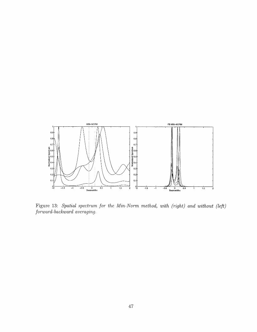
MIN-NORM FB MIN-NORM1 .1 , ,

0.9 0.9

0.8 0.8

0.7 0.7

0.67

so0.5 E 0.7

0.4°-

0.4

0.3 0.3

0.2 0.2

0.1 0.1

0 0C-2 -1.5 -1 -0.5 0 0.5 1 1.5 2 -2 -1.5 -1 -0.5 0 0.5 1 1.5 2

Beamwidths Beamwidths

Figure 13: Spatial spectrum for the Min-Norm method, with (right) and without (left)forward-backward averaging.

47

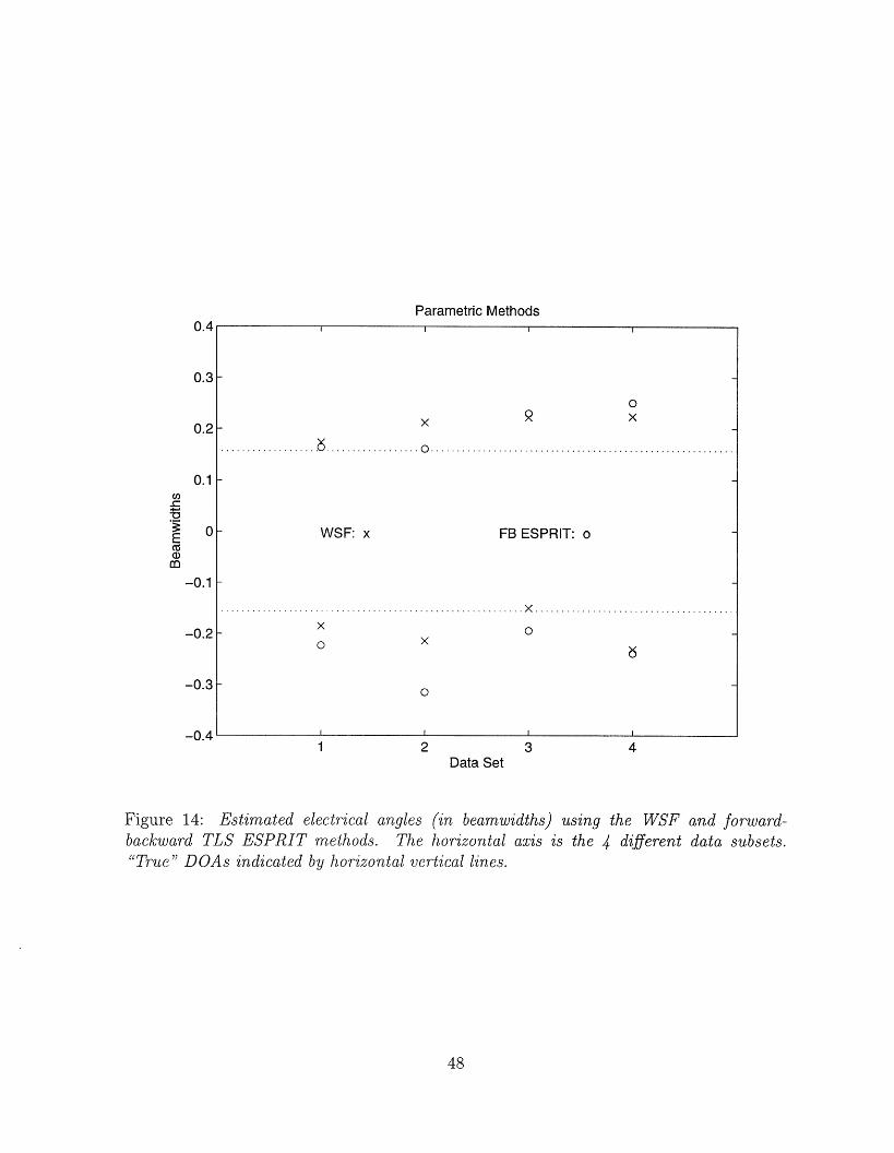
Parametric Methods0.4

0.3

0.2 - x

0.1

E - WSF: x FB ESPRIT: oE

-0.1

.. .. . .. . .. . .. .. . .. . .. .. . .. .. . .. .. . .. .. . .. .. . .. .. . . .. . .. ..X . .. . .. . .. .. . .. .. . .. . .. .. .x . . .. . .. .. . ..

-0.2 0 6 o

-0.3

-0.4 ' ' 1 2 3 4

Data Set

Figure 14: Estimated electrical angles (in beamwidths) using the WSF and forward-backward TLS ESPRIT methods. The horizontal axis is the 4 different data subsets."True" DOAs indicated by horizontal vertical lines.

48

Parametric Methods0.5 o I I I

0.4 - WSF: x FB ESPRIT: o

0.3 0o x

0.2 0 x o xx

00

X o x x-0...... ....... ° ° °

-0.2 - x .. .x 0

-0. 1 x x

-0.4 X

-0.5 I I I ,5 10 15 20 25 30

Number of Sensors

Figure 15: Estimated electrical angles (in beamwidths) using the WSF and forward-backward TLS ESPRIT methods on the entire data set A. The horizontal axis is thenumber of sensors employed by the estimator. "True" DOAs indicated by horizontal ver-tical lines.

4949

MIN-NORM FB MIN-NORM

0.9 - 0.9

0.8 0.8

0.7- 0.7E 0

0.6 0.6-

0.2 0.2

0.1 0.1

0 0-2 -1.5 -1 -0.5 0 0.5 1 1.5 2 -2 -1.5 -1 -0.5 0 0.5 1 1.5 2

Beamwidths Beamwidths

Figure 16: Spatial spectrum for the Min-Norm method, with (right) and without (left)forward-backward averaging.

50

Parametric Methods0.5

0.4WSF: x SML: o DML: +

0.3

0.2

0.1

a)cd-0.1

-0.2

-0.3

-0.4

-0.51 2 3 4 5

Data Set

Figure 17: Estimated electrical angles (in beamwidths) using the WSF, SML and DML

methods. The horizontal axis is the 4 different data subsets. "True" DOAs indicated by

horizontal vertical lines.

51

Parametric Methods0.5 , , , ,

0.4 - WSF: x SML: o DML: +

0.3+

0.2 x-

, ..... . . ..... . ........... o . .... ........... 0 ........................................ 0.1 0

02F X u1i°-00

E 0 0 0 0-0 o + ox 0

0

-0.41 X -0.2 - ~ -0.3- o +

-0.4 - X

-0.5 I I 5 10 15 20 25 30

Number of Sensors

Figure 18: Estimated electrical angles (in beamwidths) using the WSF, SML and DMLmethods on the entire data set B. The horizontal axis is the number of sensors employedby the estimator. "True" DOAs indicated by horizontal vertical lines.

52

8 Conclusions

The depth acquired from the theoretical research in sensor array processing reviewed inthis paper, have played a key role in helping identifying areas of applications. New real-world problems solvable using array signal processing techniques are regularly introduced,and it is expected that their importance will only grow as automatization becomes morewidespread in industry, and as faster and cheaper digital processing system become avail-able. This manuscript is not meant to be exhaustive, but rather as a broad review of thearea, and more importantly as a guide for a first time exposure to an interested reader.The focus is on algorithms, whereas a deeper analysis and other more specialized researchtopics are only briefly touched upon.

In concluding the recent advances of the field, we think it is safe to say that thespectral-based subspace methods and, in particular, the more advanced parametric meth-ods have clear performance improvements to offer as compared to beamforming methods.Resolution of closely spaced sources (within fractions of a beamwidth) have been demon-strated and documented in several experimental studies. However, high performance isnot for free. The requirements on sensor and receiver calibration, mutual coupling, phasestability, dynamic range, etc. become increasingly more rigorous with higher performancespecifications. Thus, in some applications the cost for achieving within-beamwidth reso-lution may still be prohibitive.

The quest for algorithms that perform well under ideal conditions and the under-standing of their properties is in some sense over with the advances over the past years.However, the remaining work is not the less challenging, namely to adapt the teoreticalmethods to fit the particular demands in specific applications. For example, real-timerequirements may place high demands on algorithm simplicity, and special array and sig-nal structures present in certain scenarios must be exploited. The future work, also inacademic research, will be much focused on bridging the gap that still exists betweentheoretical methods and real-world applications.

53

Acknowledgements

The authors are grateful to Professor S. Haykin of McMaster University for collecting thedata used in Section 7, and to Professor M. Zoltowski of Purdue University for transferingthe data. Thanks also to Dr. H. Aghajan of Stanford University for providing the figuresof Section 6.3.

54

References

[1] B.G. Agee, A.V. Schell, and W.A. Gardner. "Spectral Self-Coherence Restoral: ANew Approach to Blind Adaptive Signal Extraction Using Antenna Arrays". Proc.IEEE, 78:753-767, Apr. 1990.

[2] H.K. Aghajan and T. Kailath. Sensor Array Processing Techniques for Super Res-olution Multi-Line-Fitting and Straight Edge Detection. IEEE Trans. on ImageProc., 2(4), Oct. 1993.

[3] S. Anderson, M. Millnert, M. Viberg, and B. Wahlberg. An Adaptive Array forMobile Communication Systems. IEEE Trans. on veh. Tec., 40, 1991.

[4] T.W. Anderson. An Introduction to Multivariate Statistical Analysis, 2nd edition.John Wiley & Sons, New York, 1984.

[5] S. Andersson. "Optimal Dimension Reduction for Sensor Array Signal Processing".Signal Processing, 30(2), Jan. 1993.

[6] S.P. Applebaum. Adaptive Arrays. IEEE Trans. Antennas and Propagation,24(9):585-598, Sept. 1976.

[7] Articles. Spectra From Various Techniques. IEEE Proceedings, 69(11), 1981. SpecialIssue.

[8] Articles. Time Delay Estimation. IEEE Trans. on Acoustics, Speech and SignalProc., ASSP-29(3), June 1981. Special Issue.

[9] Articles. Spectral Estimation. IEEE Proceedings, 70(9), 1982. Special Issue.

[10] A.B. Baggeroer, W.A. Kuperman, and H. Schmidt. Matched field processing:Sourcelocalization in correlated noise as an optimum parameter estimation problem. J.Acoust. Soc. Am., 83(2):571-587, February 1988.

[11] A.J. Barabell. "Improving the Resolution Performance of Eigenstructure-BasedDirection-Finding Algorithms". In Proc. ICASSP 83, pages 336-339, Boston, MA,1983.

[12] G. Bienvenu and L. Kopp. Adaptivity to background Noise spatial coherence for highresolution passive methods. In Int. Conf. on Acoust., Speech and Signal Processing,pages 307-310, 1980.

[13] G. Bienvenu and L. Kopp. Methodes Haute Resolution Apres Formation de Voies.In Conference du GRETSI, volume 1, pages 325-330, Nice, France, May 1985.

[14] J.F. B6hme. "Estimation of Source Parameters by Maximum Likelihood and Non-linear Regression". In Proc. ICASSP 84, pages 7.3.1-7.3.4, 1984.

55

[15] J.F. Bohme. "Estimation of Spectral Parameters of Correlated Signals in Wave-fields". Signal Processing, 10:329-337, 1986.

[16] J.F. B6hme and D. Kraus. "On Least Squares Methods for Direction of ArrivalEstimation in the Presence of Unknown Noise Fields". In Proc. ICASSP 88, pages2833-2836, New York, N.Y., 1988.

[17] Y. Bresler and A. Macovski. "Exact Maximum Likelihood Parameter Estimation ofSuperimposed Exponential Signals in Noise". IEEE Trans. ASSP, ASSP-34:1081-1089, Oct. 1986.

[18] Y. Bresler and A. Macovski. "On the Number of Signals Resolvable by a UniformLinear Array". IEEE Trans. ASSP, ASSP-34:1361-1375, Oct. 1986.

[19] K. Buckley and X.-L. Xu. "Spatial-spectrum estimation in a location sector". IEEETrans. ASSP, 38:1842-1852, Nov. 1990.

[20] K.M Buckley and L.J. Griffiths. An Adaptive Generalized Sidelobe Canceller withDerivative Constraints. IEEE Trans. on Antennas and Propagation, AP-34(3):3111-319, 1986 1986.

[21] J. Burg. Maximum entropy spectral analysis. In 37th Meeting Society ExplorationGeophysicists, 1967.

[22] J.A. Cadzow. "Multiple Source Location-The Signal Subspace Approach". IEEETrans. ASSP, ASSP-38:1110-1125, July 1990.

[23] J. Capon. High-Resolution frequency-wavenumber spectrum analysis. Proc. IEEE,57(8):2408-1418, Aug. 1969.

[24] Y.-H. Chen and Y.-S. Lin. "DOA estimation by fourth-order cumulants in unknownnoise environments". In Proc. IEEE ICASSP, volume 4, pages 296-299, Minneapo-lis, MN, Apr. 1993.

[25] H. Clergeot, S. Tressens, and A. Ouamri. "Performance of High Resolution Fre-quencies Estimation Methods Compared to the Cram6r-Rao Bounds". IEEE Trans.ASSP, 37(11):1703-1720, November 1989.

[26] P. Comon and G. H. Golub. "Tracking a few Extreme Singular Values and Vectorsin Signal Processing". Proceedings of the IEEE, 78:1327-1343, Aug. 1990.

[27] J.H. Cozzens and M.J. Sousa. Source Enumeration in a Correlated Signal Envi-ronment. IEEE Trans. on Acoust., Speech and Signal Proc., 42(2):304-317, Feb.1994.

[28] R. DeGroat. "Noniterative subspace tracking". IEEE Trans on SP, 40(3):571-577,1992.

56

[29] A. Di. Multiple source location-a matrix decomposition approach. IEEE Trans. onAcoustics, Speech and Signal Processing, ASSP-33:1086-1091, Oct. 1985.

[30] S. Haykin (ed.). Array Signal Processing. Prentice-Hall, Englewood Cliffs, NJ, 1985.

[31] J. E. Evans, J. R. Johnson, and D. F. Sun. Application of Advanced Signal Process-ing Techniques to Angle of Arrival Estimation in ATC Navigation and SurveillanceSystems. Technical report, MIT Lincoln Laboratory, June 1982.

[32] A. Farina. Antenna-Based Signal Processing Techniques for Radar Systems. ArtechHouse, Norwood, MA, 1992.

[33] D.R. Farrier and L.R. Prosper. "A Signal Subspace Beamformer". In Proc. ICASSP90, pages 2815-2818, Albuquerque, NM, 1990.

[34] A.J. Fenn, C.J. Diederich, and P.R. Stauffer. An Adaptive-Focusing Algorithm fora Microwave Planar Phased-Array Hyperthermia System. The Lincoln LaboratoryJournal, 6(2):269-288, 1993.

[35] A.J. Fenn and G.A. King. "Adaptive Nulling in the Hyperthermia Treatment ofCancer. The Lincoln Laboratory Journal, 5(2):223-240, 1992.

[36] A.J. Fenn and G.A. King. Adaptive radio-frequency hyperthermia-phased arraysystem for improved cancer therapy: phantom target measurements. InternationalJournal of Hyperthermia, 10(2):189-208, March-April 1994.

[37] P. Forster. Me'thodes De Traitement d'Antenne Apr6s Filtrage Spatial. PhD thesis,Universit6 de Rennes, France, 1988.

[38] P. Forster and G. Vezzosi. "Application of Spheroidal Sequences to Array Process-ing". In Proc. ICASSP 87, pages 2268-2271, Dallas, TX, 1987.

[39] B. Friedlander. "Sensitivity Analysis of the Maximum Likelihood Direction-FindingAlgorithm". IEEE Trans. AES, AES-26(6):953-968, Nov. 1990.

[40] B. Friedlander and A. Weiss. "Direction Finding Using Spatial Smoothing withInterpolated Arrays". IEEE Trans. AES, 28:574-587, Apr. 1992.

[41] O.L. Frost. An Algorithm for Linearly Constrained Adaptive Array Processing.Proc. of the IEEE, 60(8):926-935, August 1972.

[42] W.F. Gabriel. Spectral Analysis and Adaptive Array Superresolution Techniques.Proceedings of the IEEE, 68(6):654-666, June 1980.

[43] G.H. Golub and C.F. VanLoan. "An Analysis of the Total Least Squares Problem".SIAM J. Num. Anal., 17:883-893, 1980.

57

[44] G.H. Golub and C.F. VanLoan. Matrix Computations, 2nd edition. Johns HopkinsUniversity Press, Baltimore, MD., 1989.

[45] R.P. Gooch and J. Lundel. "The CM Array: An Adaptive Beamformer for ConstantModulus Signals". In Proc. ICASSP 86, pages 2523-2526, Tokyo, Japan, 1986.

[46] N. Hirle and J.F. B6hme. Detection of knocking for Spark Ignition Engines basedon StructuralVibrations. In Int. Conf. on Acoust., Speech and Signal Processing,pages 1744-1747, 1987.

[47] S. Haykin. Radar array processing for angle of arrival estimation. In S. Haykin,editor, Array Signal Processing. Prentice-Hall, Englewood Cliffs, NJ, 1985.

[48] S. Haykin, J. Litva, and T.J. Shepherd (eds). Radar Array Processing. Springer-Verlag, Berlin, 1993.

[49] Harold Hotelling. "Analysis of a Complex of Statistical Variables into PrincipalComponents". J. Educ. Psych., 24:417-441,498-520, 1933.

[50] H. Hung and M. Kaveh. "Focussing Matrices for Coherent Signal-Subspace Pro-cessing". IEEE Trans. ASSP, ASSP-36:1272-1281, Aug. 1988.

[51] A. G. Jaffer. "Maximum Likelihood Direction Finding of Stochastic Sources: ASeparable Solution". In Proc. ICASSP 88, volume 5, pages 2893-2896, New York,New York, April 1988.

[52] Don H. Johnson and Dan E. Dudgeon. Array Signal Processing - Concepts andTechniques. Prentice-Hall, Englewood Cliffs, NJ, 1993.

[53] E. C. Jordan and K. G. Balman. Electromagnetic Waves and Radiating Systems.Prentice-Hall, New Jersey, second edition edition, 1968.

[54] I. Karasalo. "Estimating the Covariance Matrix by Signal Subspace Averaging "IEEE Trans. ASSP, ASSP-34(1):8-12, February 1986.

[55] M. Kaveh and A. J. Barabell. "The Statistical Performance of the MUSIC andthe Minimum-Norm Algorithms in Resolving Plane Waves in Noise". IEEE Trans.ASSP, ASSP-34:331-341, April 1986.

[56] M. Kaveh and A. Bassias. "Threshold extension based on a new paradigm forMUSIC-type estimation". In Proc. ICASSP 90, pages 2535-2538, Albuquerque,NM, April 1990.

[57] S.M. Kay and V. Nagesha. "Maximum Likelihood Estimation of Signals in Autore-gressive Noise". IEEE Trans on SP, 42:88-101, Jan. 1994.

[58] T. Koopmans. Linear Regression Analysis of Economic Time Series. Haarlem, DeErven F. Bohn N.V., 1937.

58

[59] D. Kraus and J.F. Bohme. "Maximum likelihood location estimation of widebandsources using the EM algorithm". In Adapt. Syst. in Contr. and Sig. Proc. 1992.Selected Papers from the 4th IFAC Symposium, pages 487-491, Grenoble, France,1993.

[60] H. Krim. Detection and Parameter Estimation of Correlated Signals in Noise. PhDthesis, North. Univ., June 1991.

[61] H. Krim. A Data-Based Enumeration of Fully Correlated Signals. IEEE Trans.Acoust., Speech, Signal Processing, July 1994.

[62] H. Krim, P. Forster, and J. G. Proakis. Operator Approach To Performance Anal-ysis Of Root-MUSIC and Root Min-Norm. IEEE Trans. Acoust., Speech, SignalProcessing, July 1992.

[63] H. Krim and J. G. Proakis. Smoothed eigenspace-based paramerter estimation.Automatica, Special Issue on Statistical Signal Procssing and Control, Jan. 1994.

[64] R. Kumaresan and D. W. Tufts. Estimating the Angles of Arrival of Multiple PlaneWaves. IEEE Trans. on Aeros. and Elect. Sys., AES-19(1), January 1983.

[65] S.Y. Kung. "A New Identification and Model Reduction Algorithm via SingularValue Decomposition". In Proc. 12th Asilomar Conf. on Circuits, Systems andComputers, pages 705-714, Pacific Grove, CA, November 1978.

[66] F. Li, J. Vaccaro, and D. W. Tufts. Min-Norm Linear Prediction For ArbitrarySensor Arrays. In Int. Conf. on Acoust., Speech and Signal Processing, pages 2613-2616, 1989.

[67] F. Li and R. Vaccaro. "Sensitivity Analysis of DOA Estimation Algorithms toSensor Errors". IEEE Trans. AES, AES-28(3):708-717, July 1992.

[68] F. Li and R.J. Vaccaro. "Performance Degradation of DOA Estimators Due toUnknown Noise Fields". IEEE Trans. SP, SP-40(3):686-689, March 1992.

[69] W.S. Liggett. Passive Sonar: Fitting Models to Multiple Time Series, volume SignalProcessing, pages 327-345. Academic Press, New York, j.w.r. griffiths and p.l.stocklin and c. vam schoonefeld edition, 1973.

[70] H. Liu, G. Xu, and L. Tong. A deterministic approach to blind equalization. InProc. of Asilomar, pages 751-755, Monterey, Nov. 1993.

[71] C.P. Mathews and M. D. Zoltowski. "Eigenstructure techniques for 2-D angle es-timation with uniform circular arrays". IEEE Trans. on SP, 42:2395-2407, Sept.1994.

[72] P. Milanfar. Geometric Estimation and Reconstruction from Tomographic Data.PhD thesis, MIT, Cambridge, MA, 1993.

59

[73] P. Milanfar, G.C. Verghese, W.C. Karl, and A.S. Willsky. Reconstructing Polygonsfrom Moments with Connections to Array Processing. IEEE Trans. on Signal Proc.,To Appear.

[74] J.S. Mosher, R.M. Leahy, and P.S. Kewis. "Biomagnetic localization from transientquasi-static events". In Proc. ICASSP 93, volume 1, pages 91-94, Minneapolis, MN,1993.

[75] B. Ottersten and T. Kailath. "Direction-of-Arrival Estimation for Wide-Band Sig-nals Using the ESPRIT Algorithm". IEEE Trans. ASSP, ASSP-38(2):317-327, Feb.1990.

[76] B. Ottersten, M. Viberg, and T. Kailath. "Analysis of Subspace Fitting and MLTechniques for Parameter Estimation from Sensor Array Data". IEEE Trans. onSP, SP-40:590-600, March 1992.

[77] B. Ottersten, M. Viberg, P. Stoica, and A. Nehorai. Exact and large sample MLtechniques for parameter estimation and detection in array processing. In Haykin,Litva, and Shepherd, editors, Radar Array Processing, pages 99-151. Springer-Verlag, Berlin, 1993.

[78] N.L. Owsley. SONAR ARRAY PROCESSING, chapter 3, pages 115-184. Haykin,Editor. Prentice Hall, Englewood Cliffs, New Jersey, 1985.

[79] A. Paulraj and T. Kailath. "Eigenstructure Methods for Direction-of-Arrival Esti-mation in the Presence of Unknown Noise Fields". IEEE Trans. on ASSP, ASSP-33:806-811, Aug. 1985.

[80] A. Paulraj, R. Roy, and T. Kailath. "A Subspace Rotation Approach to SignalParameter Estimation". Proceedings of the IEEE, pages 1044-1045, July 1986.

[81] V.F. Pisarenko. "The retrieval of harmonics from a covariance function". Geophys.J. Roy. Astron. Soc., 33:347-366, 1973.

[82] B. Porat and B. Friedlander. "Direction Finding Algorithms Based on High-OrderStatistics". IEEE Trans. SP, SP-39:2016-2024, Sept. 1991.

[83] J.G. Proakis and D.G. Manolakis. Digital Signal Processing, second edition. Macmil-lan, New York, 1992.

[84] B. D. Rao and K. V. S. Hari. Performance analysis of ESPRIT and TAM in de-termining the direction of arrival of plane waves in noise. IEEE Trans. ASSP,ASSP-37(12):1990-1995, Dec. 1989.

[85] B. D. Rao and K.V.S. Hari. Performance Analysis of Root-MUSIC. IEEE Trans.Acoust., Speech, Signal Processing, 37(12):1939-1949, December 1989.

60

[86] Y. Rockah and P. M. Schultheiss. Array shape calibration using sources in unknownlocations - Part I: Far-field sources. IEEE Trans. on ASSP, 35:286-299, March 1987.

[87] R. Roy and T. Kailath. "ESPRIT - Estimation of Signal Parameters via RotationalInvariance Techniques". IEEE Trans. on ASSP, ASSP-37(7):984-995, July 1989.

[88] Jr. R.T. Compton. Adaptive Antennas. Prentice Hall, Englewood Cliffs, NJ, 1988.

[89] S. Sakagami, S. Aoyama, K. Kuboi, S. Shirota, and A. Akeyama. "Vehicle PositionEstimates by Multibeam Antennas in Multipath Environments". IEEE Trans. onVehicular Tech., 41(1):63-68, Feb. 1992.

[90] S.V. Schell and W.A. Gardner. "Blind adaptive spatiotemporal filtering for wide-band cyclostationary signals". IEEE Trans. SP, 41:1961-1964, May 1993.

[91] R. O. Schmidt. A Signal Subspace Approach to Multiple Emitter Location andSpectral Estimation. PhD thesis, Stanford Univ., Stanford, CA, Nov. 1981.

[92] S. Shamsunder and G. Giannakis. "Signal selective localization of nonGaussiancyclostationary sources". IEEE Trans. SP, 42:2860-2864, Oct. 1994.

[93] T. J. Shan, M. Wax, and T. Kailath. On spatial smoothing for directions ofarrival estimation of coherent signals. IEEE Trans. on Acoustics, Speech and SignalProcessing, ASSp-33(4):806-811, April 1985.

[94] S. Sivanand, J.-F. Yang, and M. Kaveh. "Focusing filters for wide-band directionfinding". IEEE Trans. SP, 39:437-445, Feb. 1991.

[95] D.T.M. Slock. "Blind Fractionally-Spaced Equalization, Perfect-Reconstruction Fil-ter Banks and Multichannel Linear Prediction". In Proc. ICASSP 94, volume 4,pages 585-588, Adelaide, Australia, April 1994.

[96] K. Steiglitz and L. McBride. "A technique for identification of linear systems".IEEE Trans. Autom. Contr., AC-10:461-464, Oct. 1965.

[97] P. Stoica and A. Nehorai. "MUSIC, Maximum Likelihood and Cramer-Rao Bound".IEEE Trans. ASSP, ASSP-37:720-741, May 1989.

[98] P. Stoica and A. Nehorai. "MODE, Maximum Likelihood and Cramer-Rao Bound:Conditional and Unconditional Results". In Proc. ICASSP 90 Conf, pages 2715-2718, Albuquerque, NM, April 1990.

[99] P. Stoica and A. Nehorai. "MUSIC, Maximum Likelihood and Cramer-Rao Bound:Further Results and Comparisons". IEEE Trans. ASSP, ASSP-38:2140-2150, De-cember 1990.

61

[100] P. Stoica and A. Nehorai. "Performance Study of Conditional and UnconditionalDirection-of-Arrival Estimation". IEEE Trans. ASSP, ASSP-38:1783-1795, October1990.

[101] P. Stoica and K. Sharman. "A Novel Eigenanalysis Method for Direction Estima-tion". Proc. IEE, F:19-26, Feb 1990.

[102] P. Stoica and K. Sharman. "Maximum Likelihood Methods for Direction-of-ArrivalEstimation". IEEE Trans. ASSP, ASSP-38:1132-1143, July 1990.

[103] P. Stoica and T. S6derstr6m. "Statistical Analysis of MUSIC and Subspace RotationEstimates of Sinusoidal Frequencies". IEEE Trans. ASSP, ASSP-39:1836-1847,Aug. 1991.

[104] P. Stoica, M. Viberg, and B. Ottersten. "Instrumental Variable Approach to ArrayProcessing in Spatially Correlated Noise Fields". IEEE Trans. SP, SP-42:121-133,Jan. 1994.

[105] M. Stojanovic and Z. Zvonar. Adaptive spatial/temporal multiuser receivers fortime-varying channels with severe isi. In Proc. of Conf. on Signals and Systems,Princeton, March 1994.

[106] G. Su and M. Morf. "Modal Decomposition Signal Subspace Algorithms". IEEETrans. ASSP, ASSP-34(3):585-602, June 1986.

[107] S.C. Swales, M.A. Beach, and D.J. Edwards. "Multi-Beam Adaptive Base StationAntennas for Cellular Land Mobile Radio Systems". In Proc. IEEE Veh. Technol.Conf., pages 341-348, 1989.

[108] A. Swindlehurst and T. Kailath. "A Performance Analysis of Subspace-Based Meth-ods in the Presence of Model Errors - Part I: The MUSIC Algorithm". IEEE Trans.SP, SP-40(7):1758-1774, July 1992.

[109] A. Swindlehurst and T. Kailath. "A Performance Analysis of Subspace-Based Meth-ods in the Presence of Model Errors: Part 2 - Multidimensional Algorithms". IEEETrans. on SP, SP-41:2882-2890, Sept. 1993.

[110] S. Talwar, M. Viberg, and A. Paulraj. "Estimating Multiple Co-Channel DigitalSignals Using an Antenna Array". IEEE SP Letters, 1:29-31, Feb. 1994.

[111] L. Tong, G. Xu, and T. Kailath. "A New Approach to Blind Identification andEqualization of Multipath Channels". IEEE Trans. on Inf. Theory, To appear.

[112] H. L. Van Trees. Detection, Estimation and Modulation Theory, part. I. J. Wiley& Sons Inc., 1968.

62

[113] D. W. Tufts and R. Kumaresan. Estimation of frequencies of multiple Sinusoids:Making Linear Prediction Perform Like Maximum Likelihood. IEEE Proceedings,70(9), September 1982.

[114] F. Tuteur and Y. Rockah. "A New Method for Detection and Estimation Usingthe Eigenstructure of the Covariance Difference". In Proc. ICASSP 88 Conf, pages2811-2814, Tokyo, Japan, 1986.

[115] B.D. VanVeen and K.M. Buckley. Beamforming:A Versatile Approach to SpatialFiltering. Signal Proc. Magazine, pages 4-24, April 1988.

[116] B.D. Van Veen and B. Williams. "Dimensionality Reduction in High ResolutionDirection of Arrival Estimation". In Proc. Asilomar Conf. Sig., Syst., Comput.,Pacific Groove, CA, Oct. 1988.

[117] M. Viberg and B. Ottersten. "Sensor Array Processing Based on Subspace Fitting".IEEE Trans. SP, SP-39(5):1110-1121, May 1991.

[118] M. Viberg, B. Ottersten, and T. Kailath. "Detection and Estimation in SensorArrays Using Weighted Subspace Fitting". IEEE Trans. SP, SP-39(11):2436-2449,Nov. 1991.

[119] M. Viberg and A.L. Swindlehurst. "A Bayesian Approach to Auto-Calibration forParametric Array Signal Processing". IEEE Trans. SP, 42, Dec. 1994.

[120] M. Viberg and A.L. Swindlehurst. "Analysis of the Combined Effects of FiniteSamples and Model Errors on Array Processing Performance". IEEE Trans. SP,42:3073-3083, Nov. 1994.

[121] Mats Viberg. "Sensitivity of Parametric Direction Finding to Colored Noise Fieldsand Undermodeling". Signal Processing, 34(2):207-222, Nov. 1993.

[122] M. Wax. Detection and Estimation of Superimposed Signals. PhD thesis, StanfordUniv., Stanford, CA, March 1985.

[123] M. Wax. "Detection and Localization of Multiple Sources in Noise with UnknownCovariance". IEEE Trans. on ASSP, ASSP-40(1):245-249, Jan. 1992.

[124] M. Wax and T. Kailath. Detection of Signals by Information Theoretic Crite-ria. IEEE Trans. on Acoustics, Speech and Signal Processing, ASSP-33(2):387-392,February 1985.

[125] M. Wax, T.J. Shan, and T. Kailath. "Spatio-Temporal Spectral Analysis by Eigen-structure Methods". IEEE Trans. ASSP, ASSP-32, Aug. 1984.

[126] M. Wax and I. Ziskind. "On Unique Localization of Multiple Sources by PassiveSensor Arrays". IEEE Trans. on ASSP, ASSP-37(7):996-1000, July 1989.

63

[127] A. J. Weiss and B. Friedlander. "Array Shape Calibration Using Sources in Un-known Locations - A Maximum Likelihood Approach". IEEE Trans. on ASSP,37(12):1958-1966, Dec. 1989.

[128] B. Widrow, K. M. Duvall, R. P. Gooch, and W. C. Newman. Signal CancellationPhenomena in Adaptive Antennas: Causes and Cures. IEEE Trans. Antennas andPropagation, AP-30(5):469-478, July 1982.

[129] N. Wiener. Extrapolation, Interpolation and Smoothing of Stationary Time Series.MIT Press, Cambridge, MA, 1949.

[130] J.H. Winters. "Optimum combining for indoor radio systems with multiple users".IEEE Trans. Communications, 35:1222-1230, 1987.

[131] K.M. Wong, J.P. Reilly, Q. Wu, and S. Qiao. "Estimation of the Directions ofArrival of Signals in Unknown Correlated Noise, Parts I and II". IEEE Trans. onSP, SP-40:2007-2028, Aug. 1992.

[132] Q. Wu and K.M. Wong. "UN-MUSIC and UN-CLE: An Application of GeneralizedCanonical Correlation Analysis to the Estimation of the Directions of Arrival".IEEE Trans. SP, 42, Sept. 1994.

[133] G. Xu and T. Kailath. "Direction-of-arrival estimation via exploitation ofcyclostationary-a combination of temporal and spatial processing". IEEE Trans.SP, 40(7):1775-1786, July 1992.

[134] G. Xu and T. Kailath. "Fast Subspace Decomposition". IEEE Trans. SP, 42(3):539-551, March 1994.

[135] W. Xu and M. Kaveh. "Design of signal-subspace cost functionals for parameterestimation". In Proc. ICASSP 92, volume 5, pages 405-408, San Francisco, CA,Mar. 1992.

[136] W. Xu, J. Pierre, and M. Kaveh. "Practical detection with calibrated arrays". InProc. 6:th SP Workshop on Statistical Signal and Array Processing, pages 82-85,Victoria, Canada, Oct. 1992.

[137] X.-L. Xu and K. Buckley. "Bias analysis of the MUSIC location estimator". IEEETrans. SP, 40(10):2559-2569, Oct. 1992.

[138] X.-L. Xu and K. Buckley. "An analysis of beam-space source localization". IEEETrans. SP, 41(1):501-504, Jan. 1993.

[139] J.-F. Yang and M. Kaveh. "Adaptive eigensubspace algorithms for direction orfrequency estimation and tracking". IEEE Trans. ASSP, 36(2):241-251, Feb. 1988.

[140] L.C. Zhao, P.R. Krishnaiah, and Z.D. Bai. "On Detection of the Number of Signalsin Presence of White Noise". J. of Multivariate Analysis, 20:1:1-25, 1986.

64

[141] I. Ziskind and M. Wax. "Maximum Likelihood Localization of Multiple Sources byAlternating Projection". IEEE Trans. on ASSP, ASSP-36:1553-1560, Oct. 1988.

[142] M.D. Zoltowski, G.M. Kautz, and S.D. Silverstein. "Beamspace Root-MUSIC".IEEE Trans. on SP, 41:344-364, Jan. 1993.

65