Sensor and Simulation Notes

Note 514

March 2006

Experiments with a High-Voltage Ultra-Wideband Radar Using a Directional Coupler

Lanney M. Atchley, Everett G. Farr, and Leland Bowen Farr Research, Inc.

William D. Prather

Air Force Research Laboratory, Directed Energy Directorate

Abstract We investigate here a High-Voltage (HV) Ultra-Wideband (UWB) Radar system that uses a directional coupler, which allows a single antenna to be used for both transmission and reception. We investigate both air-filled and oil-filled directional couplers. We test the system at both low and high voltages. We compare the performance of our system to a comparable one using two separate antennas without a directional coupler. We also investigate the usefulness of limiters in protecting the oscilloscope. These tests provide insight into fundamental questions about UWB radar, such how best to isolate the receiver from the transmitter, and how to determine the highest useful source voltage.

2

CONTENTS

1. Introduction........................................................................................................................ 3 2. Single Antenna Radar Measurements at Low Voltage ...................................................... 4 2.1 Air-Filled Directional Coupler (Prototype 5) Using Attenuators .......................... 4 2.2 Oil-Filled Directional Coupler (Prototype 6) Using Attenuators .......................... 5 2.3 Air Directional Coupler (Prototype 5) with Agilent Model 11867A Limiter........ 8 2.4 Air Directional Coupler (Prototype 5) with Agilent Model 11930B Limiter...... 10 3. Dual Antenna Radar Measurements at Low Voltage ...................................................... 14 3.1 Dual Antenna Experiments Without Absorber Foam.......................................... 14 3.2 Dual Antenna Experiments Using Absorber Foam ............................................. 18 4. High Voltage Radar Experiments with the Oil Directional Coupler and IRA-6 ............. 22 5. Discussion........................................................................................................................ 26 6. Conclusions...................................................................................................................... 26 References........................................................................................................................ 27

3

1. Introduction In this paper we carry out experiments on a High-Voltage (HV) Ultra-Wideband (UWB) radar system using a single antenna with a directional coupler. In doing so, we bring together a number of circuit elements that have been described in recent papers. These include a HV UWB directional coupler [1, 2], commercially available limiters [3], the IRA-6 impulse radiating antenna [4] with diameter of 1.5 m, and an FID model FPG 30-1KM pulser with 25 kV peak voltage. The purpose of this series of experiments is to evaluate the effectiveness of our directional couplers in UWB radar systems. At the same time, we investigate a number of related issues, including the maximum useful voltage of such a system, the usefulness of limiters, and how such a system compares with a similar system using two different antennas for transmission and reception. We have developed several directional couplers in [1, 2], and we investigate the use of two of them in the experiments described here. The two that are investigated are Prototype 5, which is air-filled, and Prototype 6, which is oil-filled. We evaluate several functional impulse radar systems configured from available instrumentation. We then test our best high-voltage configuration using the FID high voltage pulser generator with the IRA-6. Our goal is to find the system which allows us to detect radar targets at the greatest distance with the highest signal-to-noise ratio (SNR). Our approach is to test various basic configurations of impulse transmitting and receiving systems to find the best possible combination of our instrumentation. Radar configurations discussed here include the following

• Single antenna systems, using both the air-filled and oil filled directional couplers and attenuators to protect the oscilloscope

• Single antenna systems, using limiters to protect the oscilloscope • Dual antenna system, without a directional coupler, and without absorber foam • Dual antenna system, with absorber foam to isolate the two antennas.

We begin our investigation with single-antenna radar measurements operating at low voltage.

4

2. Single Antenna Radar Measurements at Low Voltage We begin with low-voltage measurements using a directional coupler with a single small antenna, in order to learn as much as possible before going to higher voltages. In these experiments our antenna is either an IRA-3M or IRA-4, as described in [5], with a diameter of 46 cm (18 in.). Our source is the Kentech model ASG1, with risetime of 100 ps, peak voltage of 230 V, and long exponential decay. A plot of the output waveform of the ASG1 is shown in [2, Figure 4.9]. Our target is a metal cylinder, 30.5 cm (1 ft.) in length and 6.4 mm (1/4 in.) in diameter, which resonates near 400 MHz. 2.1 Air-Filled Directional Coupler (Prototype 5) Using Attenuators In our first test, we measured the return signal as a function of distance using a single antenna and the air-filled directional coupler, Prototype 5. The target was placed 30.5 cm (1 ft.) from the feed point of the IRA. We then moved the target away from the IRA in increments of 30.5 cm (1 ft.) out to a maximum distance of 1.52 m (5 ft.). Figure 2.1 shows the instrumentation and target setup. The output from the Kentech model ASG1 Pulse Generator is fed through the directional coupler to the IRA-4. The signal returned from the target is directed through the directional coupler, through a 20 dB attenuator and into the oscilloscope. The oscilloscope is a Tektronix model TDS6804B single-shot scope with bandwidth of 8 GHz and sampling rate of 20 gigasamples per second. The attenuator was used as a protection device for the scope, to keep the early-time leakage into the scope less than 5 V. We processed the data with simple background subtraction, recording the returned signal with and without the target in place. Background subtraction was carried out within the scope, in order to observe the target in near real time. For both waveforms, we averaged 1000 waveforms, which eliminated as much noise as possible.

IRA 4 12 inch Target

DielectricCantileverTDS6804B

Directional Coupler

50W

ASG1

20 dB

Ω

Figure 2.1. Fundamental Instrumentation Setup.

5

The time domain target returns, after background subtraction, are shown in Figure 2.2, as a function of target distance. We observe that there is little signal remaining with the target positioned just 1.5 m (5 ft) from the antenna.

0 10 20 30 40 50

-0.06

-0.04

-0.02

0

0.02

0.04

30.5 cm target, 30 cm separation

Time (ns)

Ret

urns

(vol

ts)

0 10 20 30 40 50

-0.06

-0.04

-0.02

0

0.02

0.04

30.5 cm target, 61 cm separation

Time (ns)

Ret

urns

(vol

ts)

0 10 20 30 40 50

-0.06

-0.04

-0.02

0

0.02

0.04

30.5 cm target, 91 cm separation

Time (ns)

Ret

urns

(vol

ts)

0 10 20 30 40 50

-0.06

-0.04

-0.02

0

0.02

0.04

30.5 cm target, 122 cm separation

Time (ns)

Ret

urns

(vol

ts)

0 10 20 30 40 50

-0.06

-0.04

-0.02

0

0.02

0.04

30.5 cm target, 152 cm separation

Time (ns)

Ret

urns

(vol

ts)

Figure 2.2. Radar signal strength as a function of target distance, shown in the time domain.

Next, we calculated the Fourier Transform of the time domain radar returns, and the result is shown in Figure 2.3. We expect a 30.5 cm target to resonate near 400 MHz, including

6

corrections for fatness of the rod. One can see the 400 MHz resonance in the first four measurements, but there is little left of the resonance in the final measurement at 1.5 meters (5 ft.)

10-1

100

101

10-3

10-2

10-1

100

30.5 cm Target, 30 cm separation

Frequency (GHz)

Sig

nal (

V/G

Hz)

10-1

100

101

10-3

10-2

10-1

100

30.5 cm Target, 61 cm separation

Frequency (GHz)

Sig

nal (

V/G

Hz)

10-1

100

101

10-3

10-2

10-1

100

30.5 cm Target, 91 cm separation

Frequency (GHz)

Sig

nal (

V/G

Hz)

10-1

100

101

10-3

10-2

10-1

100

30.5 cm Target 122 cm separation

Frequency (GHz)

Sig

nal (

V/G

Hz)

10-1

100

101

10-3

10-2

10-1

100

30.5 cm Target 152 cm separation

Frequency (GHz)

Sig

nal (

V/G

Hz)

Figure 2.3. Radar signal strength as a function of target distance, shown in the frequency-

domain.

We conclude that, at least over a limited distance, this basic system and primitive data processing identifies a target in both the time and frequency domains.

7

2.2 Oil-Filled Directional Coupler (Prototype 6) Using Attenuators Next, we duplicate the measurements of the previous section, with the sole change that the oil-filled directional coupler (Prototype 6) replaces air-filled directional coupler (Prototype 5). This allows us to compare results obtained with the two couplers. However, note that we carry out the measurements only at a single target distance. The time domain and frequency domain results observed at a distance of 30.5 cm (1 ft.) are given in Figure 2.3. We observe that the oil-filed coupler provides a somewhat higher signal-to-noise ratio (SNR).

0 10 20 30 40 50-0.1

-0.05

0

0.05

0.1Air coupler 30.5 cm target, 10k averages

Time (ns)

Ret

urns

(vol

ts)

0 10 20 30 40 50-0.1

-0.05

0

0.05

0.1Oil Coupler 30.5 cm target, 1k averages

Time (ns)

Ret

urns

(vol

ts)

10-1

100

101

10-3

10-2

10-1

100

ADC 30.5 cm Target

Frequency (GHz)

Sig

nal (

volts

/Hz)

10-1

100

101

10-3

10-2

10-1

100

ODC 30.5 cm Target

Frequency (GHz)

Sig

nal (

volts

/Hz)

Figure 2.3. Target return comparison between the air-filled directional coupler (Prototype 5), left,

and the and oil-filled directional coupler, right. We were surprised to observe the somewhat better performance of the oil-filled coupler, because we normally expect that a component designed for higher-voltage would exhibit compromises in performance. To determine the cause, we examined the port reflection and transmission properties of these two directional couplers, as described in [2]. We found that the oil coupler impedances are not smoother or closer to the design impedance of 50 ohms than those of the air coupler. Indeed the air coupler looks somewhat smoother. Furthermore, the output

8

voltages observed when driving Port 1 with the Kentech model ASG1 were quite comparable between the two versions. The somewhat better radar performance of the oil coupler over the air coupler remains something of a mystery, but overall, we consider the two couplers to have approximately comparable performance. 2.3 Air Directional Coupler (Prototype 5) with Agilent Model 11867A Limiter Next, we investigated the use of limiters, in an effort towards reducing or eliminating the 20 dB attenuators used in the previous sections. These attenuators reduce the received target return voltage, which limits the SNR of the system. We had previously investigated the transient performance of several commercial limiters in [3], where we found two limiters that might have acceptable performance, the Agilent models 11867A and 11930B. We therefore tried each of those in our system, as described in this section and the next. First we tested the Agilent model 11867A limiter, as shown in Figure 2.4. We made two measurements, both with and without the limiter. We introduced an attenuator just before the TDS6804B oscilloscope, and we selected its value so that the prompt leakage signals were about the same amplitude. That amplitude was chosen to be just below the peak voltage allowed by the oscilloscope – about 5 V. As before, we used background subtraction, and we placed the 30.5-cm target at a distance of one meter from the IRA-3 feed point.

IRA 3 12 inch Target

DielectricCantileverTDS6804B

Directional Coupler

50W

ASG1

11867AΩ

Attenuator

Figure 2.4. Instrumentation configuration with limiter. The background signals for the configurations with and without the limiter are shown in Figure 2.5, where we observe more noise when using the limiter. In Figure 2.6 we show the target return data after background subtraction, where we see the radar return starts at about 25 ns. The data taken with the limiter is very noisy, and is of poor quality. The Fourier transform of the return data is shown in Figure 2.7. We estimate that the data taken with the limiter has at least a 10 dB lower SNR than the data taken with an attenuator only.

9

0 10 20 30 40 50-4

-3

-2

-1

0

1

2

3

Time (ns)

Ret

urns

(vol

ts)

0 10 20 30 40 50-3

-2

-1

0

1

2

Time (ns)

Ret

urns

(vol

ts)

Figure 2.5. Comparison between attenuator-only (left) and limiter (right) background data.

0 10 20 30 40 50-0.06

-0.04

-0.02

0

0.02

0.04

Time (ns)

Ret

urns

(vol

ts)

0 10 20 30 40 50-0.04

-0.02

0

0.02

0.04

0.06

Time (ns)

Ret

urns

(vol

ts)

Figure 2.6. Comparison between attenuator-only (left) and limiter (right) return data.

10-1

100

101

10-3

10-2

10-1

100

Frequency (GHz)

Sig

nal (

volts

/GH

z)

10-1

100

101

10-3

10-2

10-1

100

Frequency (GHz)

Sig

nal (

volts

/GH

z)

Figure 2.7. Comparison between attenuator-only (left) and limiter (right) data FFTs.

A possible reason for the poor performance of the 11867A limiter is that the returned signal was superimposed on top of a background signal that was 0.5–1 V in magnitude. Recall from [3] that the limiting threshold of the 11867A is around 0.5 V. Higher voltage signals get compressed above that level, which causes a problem when subtracting two waveforms to find a

10

small signal buried in noise. To remedy this problem, we next try a limiter with a higher limiting threshold, the Agilent model 11930A. 2.4 Air Directional Coupler (Prototype 5) with Agilent Model 11930B Limiter Next, we replaced the Agilent model 11867A limiter used in the previous section with the Agilent model 11930B limiter, as shown in Figure 2.8. The 11930B has a limiting threshold of around 5 V, instead of 0.5 V, so it should be a better match for our system. The target is placed two meters from the IRA-3 feed point, so the target return is smaller than in the previous test with the 11867A, which had a target distance of 1 m. This ultimately makes no difference, because we only compare waveforms taken at the same distance.

11930Battn

IRA-3

Target

DielectricCantileverTDS6804B

AirDirectional Coupler

50W

ASG12 m

(30.5 cm)Ω

Figure 2.8. Test configuration.

We first recorded the baseline and target return without the limiter using a 12 dB attenuator. Next we replaced the 12 dB attenuator with the limiter and a 6 dB attenuator. Some attenuation is necessary after the limiter to keep the scope voltage from exceeding 5 V, because the 11930B limiter provides only soft limiting (like every other limiter we have tested) rather than hard limiting. In Figure 2.9 we compare the two baselines, and in Figure 2.10 we compare the two target returns. In Figure 2.10 the data recorded with the limiter appear to have a factor-of-two higher SNR than the data taken with the 12-dB attenuator. However, the Fourier transformed data, shown in Figure 2.11, really do not show a 6 dB improvement in SNR. In fact the transformed data show some spurious frequency resonances around 2 GHz. These resonances may be associated with ringing seen in the time domain data near 10 ns. Clearly a limiter is of little use if it introduces additional resonances, so we investigate next the source of these resonances.

11

0 10 20 30 40 50-15

-10

-5

0

5

10Baseline, 12dB

Time (ns)

Ret

urns

(vol

ts)

0 10 20 30 40 50-8

-6

-4

-2

0

2

4

6Baseline, 11930B, 6dB

Time (ns)

Ret

urns

(vol

ts)

Figure 2.9. Background measurements with the 12 dB attenuator, left, and with the 11930B limiter with 6 dB attenuator, right.

0 10 20 30 40 50-0.08

-0.06

-0.04

-0.02

0

0.02

0.04

0.0630.5 cm target, 12dB

Time (ns)

Ret

urns

(vol

ts)

0 10 20 30 40 50-0.08

-0.06

-0.04

-0.02

0

0.02

0.0430.5 cm target, 11930B, 6dB

Time (ns)

Ret

urns

(vol

ts)

Figure 2.10. Target returns: 12-dB attenuator (left), 11930B with 6 dB attenuator (right).

10-1

100

101

10-3

10-2

10-1

100

30.5 cm target, 12 dB

Frequency (GHz)

Sig

nal (

volts

/GH

z)

10-1

100

101

10-3

10-2

10-1

100

30.5 cm target, 11930B, 6 dB

Frequency (GHz)

Sig

nal (

volts

/GH

z)

Figure 2.11. FFT of target returns. Attenuator only (left), 11930B limiter plus attenuator (right).

12

Finally, we investigated whether the resonances near 2 GHz were related to the impedance mismatches introduced by the limiter. To do so, we reversed the physical position of the attenuator and limiter, placing the attenuator between the directional coupler and the limiter. With the positions reversed, the input to the oscilloscope exceeded 5 V, so we had to use a 12 dB attenuator, which is what we needed without the limiter. The time domain target return, shown in Figure 2.12, indicates that the SNR is worse than the attenuator alone, although the ringing around 10 ns has disappeared. The disappearance of the time-domain ringing is consistent with the disappearance of the resonances around 2 GHz in the Fourier transformed data, shown in Figure 2.13.

0 10 20 30 40 50-15

-10

-5

0

5

10Baseline, 12dB 11930B

Time (ns)

Ret

urns

(vol

ts)

0 10 20 30 40 50-0.08

-0.06

-0.04

-0.02

0

0.02

0.04

0.0630.5 cm target, 12 dB 11930B

Time (ns)

Ret

urns

(vol

ts)

Figure 2.12. Target return with the positions of the 12-dB attenuator and 11930B reversed, background, left, and signal after background subtraction, right.

10-1

100

101

10-3

10-2

10-1

100

30.5 cm target, 12 dB

Frequency (GHz)

Sig

nal (

volts

/GH

z)

Figure 2.13. FFT target return: 12-dB attenuator and 11930B reversed.

From these results we conclude that impedance mismatches between the limiter and the directional coupler cause spurious resonances, and that any necessary attenuation should, if possible, be placed between the coupler and the limiter. We also note that this spurious effect was much less noticeable when we used the 11867B (Figure 2.7). So, not surprisingly, these spurious signals are also dependent on the exact instrumentation used.

13

As we look at the results for the 11867A (Figure 2.7) and the 11930B (Figure 2.11) we observe that in neither case is the limiter configuration superior to the configuration using only attenuators. So our overall conclusion on limiters is that those currently available commercially are of no real value in our system. It might be useful to investigate custom designs for limiters, and it might also be useful to investigate alternatives to limiters, such as GaAs or PIN diode switches. In the section that follows, we consider how the radar data taken with directional couplers compares to data taken with two separate antennas, without directional couplers.

14

3. Dual Antenna Radar Measurements at Low Voltage Next, we investigated dual antenna radar systems, in order to assess the impact of the directional couplers on the radar system. We compared the systems of the previous section to similar systems without a directional coupler, using separate antennas for transmit and receive. This comparison provides baseline data for forming a tradeoff between the increased size of two antennas versus the reduced performance of a single antenna with directional coupler. Our measurements in this section are all made without limiters, so they are comparable to those in Sections 2.1 and 2.2. To optimize the dual antenna configuration, we investigated configurations both with and without absorber foam between the antenna. 3.1 Dual Antenna Experiments Without Absorber Foam We suspended the 30.5 cm (12 inch) target from a dielectric support positioned along the centerline between two IRAs (an IRA-3M and an IRA-4), as shown in Figure 3.1. We moved the target along the centerline and away from the IRAs, continually adjusting the pointing angle of the antennas so the target remained on boresight. The target distance ranged from 30.5 cm (1 ft.) to 3.05 m (10 ft.) in increments of 30.5 cm (1 ft.). The measurements at small distances allow a direct comparison to the data taken in the previous section with the directional coupler.

30.5 cm Target

DielectricCantilever

ASG1

IRA 3IRA 4

TDS6804BAttn

70 cm

30.5 cm

Figure 3.1. Dual IRA instrumentation setup block diagram and photograph.

15

As shown in Figure 3.1, the Kentech model ASG1 pulser (230 V peak and 100 ps rise time) drives the transmit IRA directly. We recorded the received signal from the second IRA, using an attenuator to reduce the crosstalk from the transmit antenna to about 3 volts. Initially we need 10 dB of attenuation, but we ultimately reduced it to 6 dB as the IRAs increasingly point away from each other, reducing the crosstalk. Initially, we used no absorber foam to reduce crosstalk, but we do so in the section that follows. The data processing is identical to that used in previous testing with the single antenna. We first recorded a background measurement with no target. We then placed the target on the dielectric support and recorded the target return. We subtracted the background response from the target return in the TDS6804B oscilloscope as before. In Figure 3.2 we present the data for the received signal after background subtraction, with time-domain data on the left, and frequency domain data on the right. The distance of the target from the IRAs increases in 30.5-cm steps from top to bottom of the multi-page figure. We can now compare this data with the earlier data taken with the air directional coupler in sections 2.1 and 2.2. Looking at just the 30.5-cm distance, we observed a received signal of around 50 mV with the directional coupler, and 1 V with two separate antennas. So by using two separate antennas with no directional coupler we increased the SNR by around 26 dB. Note, however, that there is usually not enough room for two separate antennas. A more fair comparison would consider the performance of a single antenna to that of two smaller antennas in close proximity.

16

0 10 20 30 40 50-1

-0.5

0

0.5

1

30.5 cm target, 1 X 30.5cm

Time (ns)

Ret

urns

(vol

ts)

10-1

100

101

10-2

10-1

100

101

30.5 cm target, 1 X 30.5cm

Frequency (GHz)

Sig

nal (

volts

/GH

z)

0 10 20 30 40 50-0.5

0

0.530.5 cm target, 2 X 30.5cm

Time (ns)

Ret

urns

(vol

ts)

10-1

100

101

10-3

10-2

10-1

100

30.5 cm target, 2 X 30.5cm

Frequency (GHz)

Sig

nal (

volts

/GH

z)

0 10 20 30 40 50

-0.2

-0.1

0

0.1

0.2

0.330.5 cm target, 3 X 30.5cm

Time (ns)

Ret

urns

(vol

ts)

10-1

100

101

10-3

10-2

10-1

100

30.5 cm target, 3 X 30.5cm

Frequency (GHz)

Sig

nal (

volts

/GH

z)

0 10 20 30 40 50-0.2

-0.15

-0.1

-0.05

0

0.05

0.1

0.15

0.230.5 cm target, 4 X 30.5cm

Time (ns)

Ret

urns

(vol

ts)

10-1

100

101

10-3

10-2

10-1

100

30.5 cm target, 4 X 30.5cm

Frequency (GHz)

Sig

nal (

volts

/GH

z)

Figure 3.2 (1 of 3). Radar backscatter in dual antenna configuration as a function of distance,

time domain (left), and frequency domain (right), (cont’d next page).

17

0 10 20 30 40 50-0.2

-0.15

-0.1

-0.05

0

0.05

0.1

0.15

0.230.5 cm target, 5 X 30.5cm

Time (ns)

Ret

urns

(vol

ts)

10-1

100

101

10-3

10-2

10-1

100

30.5 cm target, 5 X 30.5cm

Frequency (GHz)

Sig

nal (

volts

/GH

z)

0 10 20 30 40 50

-0.1

-0.05

0

0.05

0.1

0.1530.5 cm target, 6 X 30.5cm

Time (ns)

Ret

urns

(vol

ts)

10-1

100

101

10-3

10-2

10-1

100

30.5 cm target, 6 X 30.5cm

Frequency (GHz)

Sig

nal (

volts

/GH

z)

0 10 20 30 40 50-0.1

-0.05

0

0.05

0.130.5 cm target, 7 X 30.5cm

Time (ns)

Ret

urns

(vol

ts)

10-1

100

101

10-3

10-2

10-1

100

30.5 cm target, 7 X 30.5cm

Frequency (GHz)

Sig

nal (

volts

/GH

z)

0 10 20 30 40 50-0.1

-0.05

0

0.05

0.130.5 cm target, 8 X 30.5cm

Time (ns)

Ret

urns

(vol

ts)

10-1

100

101

10-3

10-2

10-1

100

30.5 cm target, 8 X 30.5cm

Frequency (GHz)

Sig

nal (

volts

/GH

z)

Figure 3.2 (2 of 3). Radar backscatter in dual antenna configuration as a function of distance,

time domain (left), and frequency domain (right) (cont’d next page).

18

0 10 20 30 40 50-0.05

0

0.0530.5 cm target, 9 X 30.5cm

Time (ns)

Ret

urns

(vol

ts)

10-1

100

101

10-3

10-2

10-1

100

30.5 cm target, 9 X 30.5cm

Frequency (GHz)

Sig

nal (

volts

/GH

z)

0 10 20 30 40 50-0.04

-0.03

-0.02

-0.01

0

0.01

0.02

0.03

0.0430.5 cm target, 10 X 30.5cm

Time (ns)

Ret

urns

(vol

ts)

10-1

100

101

10-3

10-2

10-1

100

30.5 cm target, 10 X 30.5cm

Frequency (GHz)

Sig

nal (

volts

/GH

z)

Figure 3.2 (3 of 3). Radar backscatter in dual antenna configuration as a function of distance,

time domain (left), and frequency domain (right). 3.2 Dual Antenna Experiments Using Absorber Foam Next, we introduced absorber foam into the dual antenna test of the previous section, in order to reduce antenna crosstalk. In the previous section, we established that using two antennas provides 26 dB more signal than using a single antenna with a directional coupler. Using absorber foam between the antennas should improve the dual antenna configuration even further by reducing the crosstalk. This allows a more sensitive vertical scale, thus increasing the SNR. To test the theory, we set up the equipment as shown in Figure 3.3. We acquired baseline and target data before and after placing a 61 X 61 cm slab of RF absorbing material between the two IRAs. We used Advanced Electromagnetics, Inc. AEL-4.5 with foil backing. Two slabs of thickness 11.4 cm (4.5 in.) were placed with foil sides back-to-back, as shown in Figure 3.4. First, we took baseline data without a target, shown in Figure 3.5. This demonstrates that the RF absorbing material reduces the crosstalk by about 14 dB. The lower crosstalk allowed us to change the vertical scale from 1 V per division to 200 mV per division. Next, we added the target, and the time domain radar return data are shown in Figure 3.6. The Fourier transforms of the target returns are shown in Figure 3.7. In both of these figures we observe about a 5 dB reduction in the return signal from the target, after the addition of the RF

19

absorbing material. We believe this reduction is due to the absorber being too close to the antenna, and it should be possible to reduce this number with some trial and error. If we combine the above two effects, we find that the absorber foam provided a net 9 dB advantage over a dual antenna configuration with no absorber. This is because the absorber reduced the crosstalk by about 14 dB but decreased the radar return by 5 dB. However, when examining the frequency domain data in Figure 3.7, this 9 dB advantage is not apparent. In fact, the resonances in the two graphs seem to be about the same level above the noise. This is explained by noting in the background measurements of Figure 3.5 that the configuration with foam could have been driven at a higher voltage without damaging the scope, because the crosstalk was lower. If we had done so, the advantage would have become apparent in the frequency domain data. We can now combine 9 dB advantage obtained with absorber foam with the 26 dB advantage of two antennas over a single antenna plus directional coupler found in Section 3.1. This results in a net 35 dB advantage in using two antennas with absorber foam over a single antenna with a directional coupler. In other words, our directional couplers reduce the SNR of a radar system by about 35 dB compared to what could be achieved with two antennas with absorber foam between them. While this is highly dependent upon the specific equipment used, it may serve as a useful benchmark. One must use caution when trying to extend this work to other antennas and couplers, which would have different levels of crosstalk and different directivities. Note also that a more fair comparison would have used the same aperture area in the dual antenna configuration that was available in the single antenna, for example, by using a split IRA [6]. This might be a useful area for further research. Finally, we note that there may be some advantage to positioning the two antennas at the corners of a cube as described by Baum in [7], but that was not investigated here. The theory in [7] suggests that this should reduce crosstalk at low frequencies, where the antenna is electrically small.

20

30.5 cm Target

DielectricCantilever

ASG1

IRA 4

TDS6804B

70 cm

IRA 3

2 m

Figure 3.3. Instrumentation setup.

Figure 3.4. RF absorber material placement between IRAs. Target in foreground on left.

21

0 10 20 30 40 50-2

-1

0

1

2

3

4Baseline, No RF Mat

Time (ns)

Ret

urns

(vol

ts)

0 10 20 30 40 50-0.6

-0.4

-0.2

0

0.2

0.4

0.6

0.8Baseline, RF Mat Centered

Time (ns)

Ret

urns

(vol

ts)

Figure 3.5. Baseline without (left) and with (right) RF absorbing material.

0 10 20 30 40 50-0.2

-0.15

-0.1

-0.05

0

0.05

0.1

0.1530.5 cm target, No RF Mat

Time (ns)

Ret

urns

(vol

ts)

0 10 20 30 40 50-0.1

-0.05

0

0.05

0.130.5 cm target, RF Mat Centered

Time (ns)

Ret

urns

(vol

ts)

Figure 3.6. Target (30.5 cm) return without (left) and with (right) RF absorbing material.

10-1

100

101

10-3

10-2

10-1

100

30.5 cm target, No RF Mat

Frequency (GHz)

Sig

nal (

volts

/GH

z)

10-1

100

101

10-3

10-2

10-1

100

30.5 cm target, RF Mat Centered

Frequency (GHz)

Sig

nal (

volts

/GH

z)

Figure 3.7. Fourier transform of the target return without (left) and with (right) RF absorbing material.

22

4. High Voltage Radar Testing with the Oil Directional Coupler and IRA-6 Finally we tested the complete system using a high-voltage pulse source, an oil-filled, high-voltage directional coupler and an impulse radiating antenna designed for high voltage. We protected our oscilloscope using attenuators alone, with no limiters. We measured targets of two different sizes at three different distances. The test setup is shown in Figure 4.1, and photographs of the instrumentation are shown in Figure 4.2.

FPG 30-1KM IRA6

Target

FiberglassLadder withPVCCantilever

TDS6804B Oil-filledDirectional Coupler

Attn.50W Attn.Ω

Figure 4.1. High voltage test setup.

Figure 4.2. Target stand (left); FID pulser, oil-filled directional coupler and IRA-6 back (right).

23

Figure 4.3. Front view of the IRA-6. Figure 4.4. Output of the FID model

FPG 30-1KM pulser.

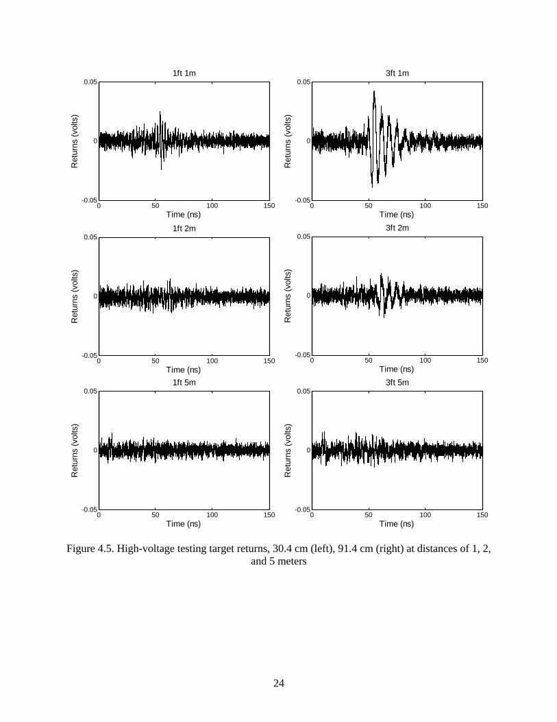
The IRA-6 antenna is a high-voltage, cable-fed, version of the standard Farr Research IRA, with diameter of 1.52 m (5 ft.). It was specially designed for this project, and is discussed in detail in [4]. A photo of the IRA-6 is shown in Figure 4.3. The pulser is an FID model FPG 30-1KM. It has a peak voltage of 25 kV, a risetime of 170 ns, and a pulse width of 2 ns. The output of this pulser was measured in [4] using a Farr Research model VDC-1 V-dot cable sensor, and the resulting output waveform is shown in Figure 4.4. We determined the attenuation by vastly over-attenuating the signal, and then reducing the attenuation until the voltage was large as possible, but still within the oscilloscope input voltage tolerance. This resulted in an attenuation of 66 dB just in front of the scope. We tested two thin-rod targets of lengths 30.5 cm (1 ft) and 91.4 cm (3 ft). We tested each target at distances of 1, 2, and 5 from the IRA-6 antenna feed. In Figure 4.5 we show the time-domain target returns. As the figure shows, the target return for the 91.4-cm target is significantly larger than that for the 30.5-cm target. Both targets are apparent in the data taken at 1- and 2-meter distances, but at 5 meters the returns are lost in the noise. Finally, we calculated the Fourier transforms of the high-voltage return data, as shown in Figure 4.6. We expect resonant frequencies of around 400 MHz for the 1-ft target and 150 MHz for the 3-ft target. The resonances are apparent at closer distances, and they fade out at larger distances, which is consistent with the time domain results.

24

0 50 100 150-0.05

0

0.051ft 1m

Time (ns)

Ret

urns

(vol

ts)

0 50 100 150-0.05

0

0.053ft 1m

Time (ns)

Ret

urns

(vol

ts)

0 50 100 150-0.05

0

0.051ft 2m

Time (ns)

Ret

urns

(vol

ts)

0 50 100 150-0.05

0

0.053ft 2m

Time (ns)

Ret

urns

(vol

ts)

0 50 100 150-0.05

0

0.051ft 5m

Time (ns)

Ret

urns

(vol

ts)

0 50 100 150-0.05

0

0.053ft 5m

Time (ns)

Ret

urns

(vol

ts)

Figure 4.5. High-voltage testing target returns, 30.4 cm (left), 91.4 cm (right) at distances of 1, 2, and 5 meters

25

10-1

100

101

10-3

10-2

10-1

100

1ft 1m

Frequency (GHz)

Sig

nal (

volts

/GH

z)

10-1

100

101

10-3

10-2

10-1

100

3ft 1m

Frequency (GHz)

Sig

nal (

volts

/GH

z)

10-1

100

101

10-3

10-2

10-1

100

1ft 2m

Frequency (GHz)

Sig

nal (

volts

/GH

z)

10-1

100

101

10-3

10-2

10-1

100

3ft 2m

Frequency (GHz)

Sig

nal (

volts

/GH

z)

10-1

100

101

10-3

10-2

10-1

100

1ft 5m

Frequency (GHz)

Sig

nal (

volts

/GH

z)

10-1

100

101

10-3

10-2

10-1

100

3ft 5m

Frequency (GHz)

Sig

nal (

volts

/GH

z)

Figure 4.6. Fourier transforms of the of high-voltage testing target returns, for target lengths of

30.4 cm (left) and 91.4 cm (right), at distances of 1, 2, and 5 meters (top to bottom).

26

5. Discussion In low-voltage radar measurements with a single antenna, the oil-filled directional coupler (Prototype 6) slightly outperformed the air-filled version (Prototype 5). This was a little surprising, because there was little difference in the port measurements of the two couplers, as shown in [2]. The difference seems unimportant until it is confirmed by additional experiments. We tried using the two commercially available limiters suggested by our earlier results in [3], but they did not improve the SNR of radar data. The Agilent model 11930B allowed us to remove some attenuation at the expense of added noise, but it also added some spurious resonances to the data, so there was no net benefit to the system. Furthermore, this limiter it is rated only to a peak voltage of 17 V, which provides only a small amount of protection beyond the 5 volts or so that an oscilloscope can already tolerate. The other limiter we tried, the Agilent model 11867A, has a limiting threshold of 0.5 V, which was too low to be useful. Because we have direct crosstalk that is around 30 dB down from the source voltage, increasing the drive voltage beyond about a few hundred volts provides no advantage in SNR. Above this voltage, extra attenuation is needed to protect the oscilloscope, so there is no net benefit. For that reason, we were unable to take full advantage of the capabilities of the 25-kV FID pulser. The best dual antenna configuration had a 35-dB advantage in SNR over the single-antenna configurations that used a directional coupler. However, there is usually not enough aperture area available for two antennas. To make optimal use of the available aperture area, one will have to either use a single antenna, or use two smaller antennas that are very closely spaced. Having two closely spaced antennas presents a challenge in reducing crosstalk, so it will be necessary to investigate configurations of two closely spaced antennas with low crosstalk. One example might be the split IRA described in [6], and there are many others. Note that we might have created a split IRA out of the IRA-6 simply by using each half of the antenna as separate transmit and receive antennas. But this would have created a problem with impedance matching, because each half has an impedance of 100 Ω instead of 50 Ω, so further research will be necessary to reduce the effect of multiple bounces. In parallel with this work, we have continued the push toward higher directivities in directional couplers, as reported in [2]. As a result, we have achieved some improvement, but our maximum directivity remains no better than 33 dB. 6. Conclusions We have successfully set up a UWB radar system with a directional coupler and detected a half-wave resonance in a wire dipole. The system was able to detect the target only at very small distances, due to the limited directivity of the directional coupler. The limited directivity allows an early-time leakage directly into the oscilloscope, causing a voltage spike. To protect the scope, we had to use attenuators that reduced the SNR.

27

To increase the range of a UWB radar, it will not be sufficient to simply use a higher voltage source. When using the 25 kV source in the measurements described here, it was necessary to use 66 dB of attenuation at the input to the oscilloscope. Doing so offsets any benefit of the higher voltage. Thus, solving the problem of early-time leakage is critical to increasing the range of the radar. To reduce the early-time leakage into the oscilloscope one would want to investigate one or more of the following four approaches. First, one could increase the directivity of the coupler, but after trying many different variations of the current design, it seems likely that a new design will be required. Second, one could use a better limiter than those currently available commercially, but this will require a custom design. Third, one could use a GaAs or PIN diode switch to time-gate the early-time leakage. But one will have to characterize these nonlinear devices for distortions that could be introduced into the signal, as we did for the limiter in [3]. Finally, one could investigate the use of two closely spaced antennas that are designed to have low crosstalk. Acknowledgements We wish to thank Dr. Carl E. Baum for helpful discussions on this topic. We wish to thank Dr. John Aurand of ITT Industries, who shared with us his thoughts on GaAs and PIN diode switches. We also wish to thank the Air Force Research Laboratory, Directed Energy Directorate, for funding this work. References 1. L. M. Atchley, E. G. Farr, D.E. Ellibee and D.I Lawry, A High-Voltage UWB Coupled-

Line Directional Coupler, Sensor and Simulation Note 489, April 2004.

2. L. M. Atchley, L. H. Bowen, E. G. Farr, D. E. Ellibee, and W. D. Prather, Further Developments in High-Voltage UWB Directional Couplers, Sensor and Simulation Note 513, March 2006.

3 L. M. Atchley, E. G. Farr, W. D. Prather, The Response of Commercial Limiters to Transient Signals, Measurement Note 59, April 2005.

4. L. H. Bowen, E. G. Farr, and W. D. Prather, A High-Voltage Cable-Fed Impulse Radiating Antenna, Sensor and Simulation Note 507, December 2005.

5. L. H. Bowen, E. G. Farr, C. E. Baum, T. C. Tran, and W. D. Prather, Results of Optimization Experiments on a Solid Reflector IRA, Sensor and Simulation Note 463, January 2002.

6. E. G. Farr and C. E. Baum, Impulse Radiating Antennas With Two Refracting or Reflecting Surfaces, Sensor and Simulation Note 379, May 1995.

7. C. E. Baum, Location and Orientation of Electrically Small Transmitting and Receiving Antenna Pairs with Common Linear Polarization and Beam Direction for Minimal Mutual Coupling, Sensor and Simulation Note 446, March 2000.