Sensfusion

ThomasBak

LectureNotes- EstimationandSensorInformationFusion

November14,2000

Aalborg UniversityDepartmentof ControlEngineeringFredrikBajersVej 7CDK-9220AalborgDenmark

2 Tableof Contents

Table of Contents

1. Intr oduction �� 3

2. Sensors �� 42.1 SensorClassification. . . . . . . . . . . . . . . . . . . . . . . . . . . . . . . . . . . . . . . . 42.2 Multiple SensorNetworks . . . . . . . . . . . . . . . . . . . . . . . . . . . . . . . . . . . 5

3. Fusion �� 63.1 Levelsof SensorFusion. . . . . . . . . . . . . . . . . . . . . . . . . . . . . . . . . . . . . 63.2 An I/O-BasedCharacterization. . . . . . . . . . . . . . . . . . . . . . . . . . . . . . . 73.3 CentralversusDecentralFusion . . . . . . . . . . . . . . . . . . . . . . . . . . . . . . 7

4. Multiple Model Estimation �� 104.1 Benefitsof Multiple Models. . . . . . . . . . . . . . . . . . . . . . . . . . . . . . . . . . 104.2 ProblemFormulation . . . . . . . . . . . . . . . . . . . . . . . . . . . . . . . . . . . . . . . 124.3 Methodsof Multi-Model Estimation. . . . . . . . . . . . . . . . . . . . . . . . . . . 13

4.3.1 Model SwitchingMethods . . . . . . . . . . . . . . . . . . . . . . . . . . . . 134.3.2 TheModel DetectionMethod. . . . . . . . . . . . . . . . . . . . . . . . . . 144.3.3 Multiple HypothesisTesting. . . . . . . . . . . . . . . . . . . . . . . . . . . 164.3.4 Model Fusion . . . . . . . . . . . . . . . . . . . . . . . . . . . . . . . . . . . . . . . 184.3.5 CombinedSystem . . . . . . . . . . . . . . . . . . . . . . . . . . . . . . . . . . . 23

1. Introduction 3

1. Intr oduction

This notediscussesmulti-sensorfusion. Throughsensorfusion we may combinereadingsfrom differentsensors,remove inconsistenciesandcombinethe informa-tion into onecoherentstructure.This kind of processingis a fundamentalfeatureof all animalandhumannavigation, wheremultiple informationsourcessuchasvision,hearingandbalancearecombinedto determinepositionandplanapathto agoal.

While theconceptof datafusionis not new, theemergenceof new sensors,ad-vancedprocessingtechniques,andimproved processinghardwaremake real-timefusion of dataincreasinglypossible.Despiteadvancesin electroniccomponents,however, developingdataprocessingapplicationssuchasautomaticguidancesys-temshasproveddifficult. Systemsthatarein directcontactandinteractwith therealworld, requirereliableandaccurateinformationabouttheir environment.This in-formationis acquiredusingsensors,thatis devicesthatcollectdataabouttheworldaroundthem.

The ability of oneisolateddevice to provide accuratereliabledataof its envi-ronmentis extremelylimited astheenvironmentis usuallynot very well definedinadditionto sensorsgenerallynot beingavery reliableinterface.

Sensorfusionseeksto overcomethedrawbacksof currentsensortechnologybycombininginformationfrom many independentsourcesof limited accuracy andre-liability to giveinformationof betteraccuracy andreliability. Thismakesthesystemlessvulnerableto failuresof a singlecomponentandgenerallyprovide moreaccu-rateinformation.In additionseveral readingsfrom thesamesensorarecombined,makingthesystemlesssensitive to noiseandanomalousobservations.

4 2. Sensors

2. Sensors

2.1 SensorClassification

Sensorsmaybe classifiedinto two groups:activeor passive. Activesensorssendsa signal to the environmentandmeasuresthe interactionbetweenthis signalandthe environment.Examplesincludesonarand radar. By contrast,passivesensorssimply recordsignalsalreadypresentin the environment.Passive sensorsincludemostthermometersandcameras.

Sensorsmayalsobeclassifiedaccordingto themediumusedfor measuringtheenvironment.This typeof classificationis relatedto thesenseswith which humansarenaturallyendowed.

Electromagneticsensors (Humanvision).

1. ChargedCoupledDevices(CCD)2. RadioDetectionandRanging(RADAR)3. ect.

Soundwavesensors (Humanhearing).

1. SoundNavigationandRanging(SONAR)2. ect.

Odorsensors (Humansmell).

Touch sensors.

1. Bumpers2. Light EmittingDiodes(LED)3. ect.

Proprioceptivesensors (Humanbalance).Thesensesthattell thebodyof its posi-tion andmovementarecalledproprioceptivesenses.Examples:

1. Gyroscopes2. Compass3. GPS4. ect.

2.2 Multiple SensorNetworks 5

2.2 Multiple SensorNetworks

Multiple sensornetworksmaybeclassifiedby how thesensorsin thenetwork inter-act.Threeclassesaredefined:

Complementary. Sensorsare complementarywhen they do not dependon eachotherdirectly, but canbe combinedto give a morecompleteimageof the en-vironment.Complementarydatacan often be fusedby simply extendingthelimits of thesensors.

Competitive. Sensorsare competitive when they provide independentmeasure-mentsof thesameinformation.They provideincreasedreliability andaccuracy.Becausecompetitivesensorsareredundant,inconsistenciesmayarisebetweensensorreadings,andcaremustbe taken to combinethe datain away that re-movestheuncertainties.Whendoneproperly, thiskind of datafusionincreasestherobustnessof thesystem.

Cooperative. Sensorsare cooperative when they provide independentmeasure-ments,that when combinedprovide information that would not be availablefrom any onesensor. Cooperative sensornetworks take datafrom simplesen-sorsandconstructa new abstractsensorwith datathat doesnot resemblethereadingsfrom any onesensor.

Themajorfactorsdictatingtheselectionof sensorsfor fusionare:thecompati-bility of thesensorsfor deploymentwithin thesameenvironment,andthecomple-mentarynatureof the informationderivedfrom thesensors.If thesensorsweretomerelyduplicatetheinformation,thethefusionprocesswouldmerelybetheequiv-alent of building in redundancy for the enhancementof reliability of the overallsystem.

Ontheotherhand,thesensorsshouldbecomplementaryenoughin termsof suchvariablesasdatarates,field of view, range,sensitivity to makefusionof informationmeaningful.

6 3. Fusion

3. Fusion

3.1 Levelsof SensorFusion

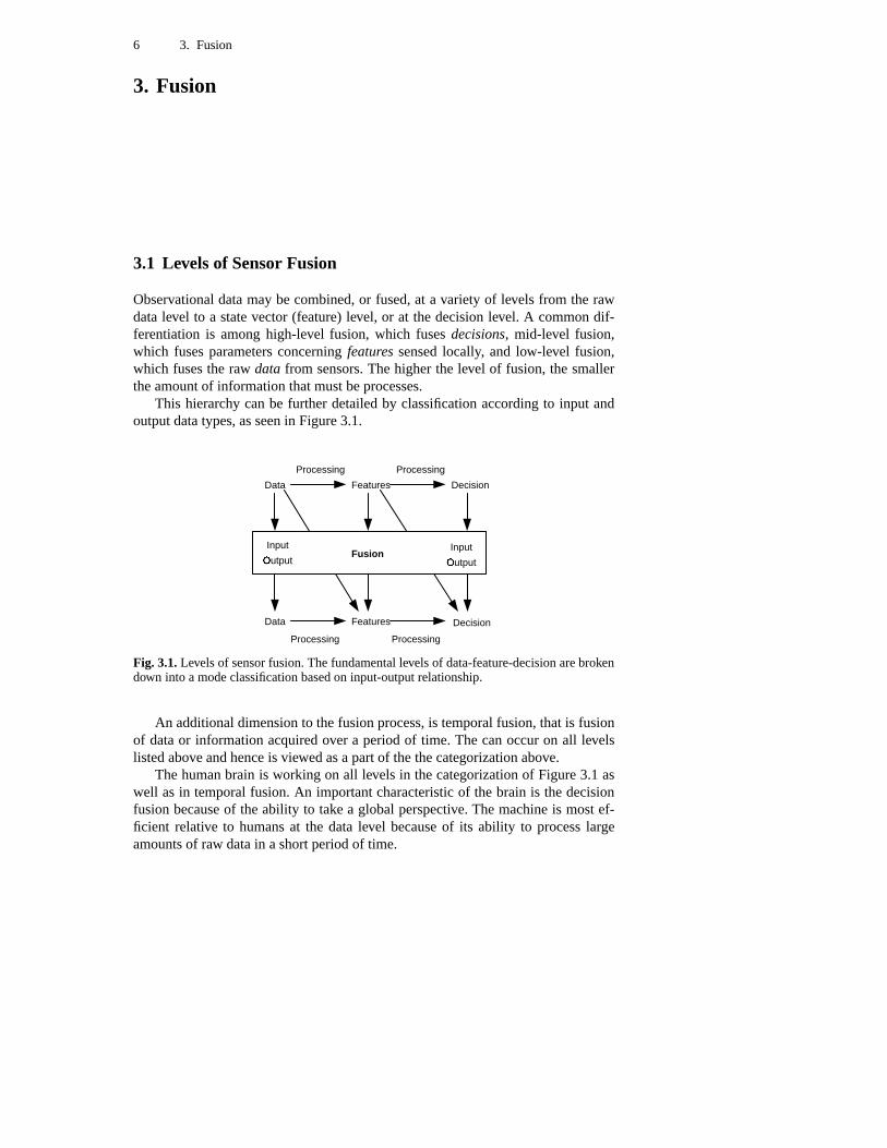
Observationaldatamaybecombined,or fused,at a varietyof levels from the rawdatalevel to a statevector(feature)level, or at the decisionlevel. A commondif-ferentiationis amonghigh-level fusion, which fusesdecisions, mid-level fusion,which fusesparametersconcerningfeaturessensedlocally, and low-level fusion,which fusesthe raw data from sensors.Thehigherthe level of fusion, the smallertheamountof informationthatmustbeprocesses.

This hierarchycanbe further detailedby classificationaccordingto input andoutputdatatypes,asseenin Figure3.1.

Data Features Decision

Data Features

Processing Processing

Processing Processing

Decision

Input

Output � Input

Output �Fusion

Fig. 3.1.Levelsof sensorfusion.Thefundamentallevelsof data-feature-decisionarebrokendown into a modeclassificationbasedon input-outputrelationship.

An additionaldimensionto thefusionprocess,is temporalfusion,thatis fusionof dataor informationacquiredover a periodof time. The canoccuron all levelslistedaboveandhenceis viewedasa partof thethecategorizationabove.

Thehumanbrain is working on all levels in thecategorizationof Figure3.1 aswell asin temporalfusion.An importantcharacteristicof the brain is thedecisionfusionbecauseof theability to take a globalperspective.Themachineis mostef-ficient relative to humansat the datalevel becauseof its ability to processlargeamountsof raw datain ashortperiodof time.

3.2 An I/O-BasedCharacterization 7

3.2 An I/O-BasedCharacterization

By characterizingthethreefundamentallevels in Figure3.1,data-feature-decisionby their input outputrelationshipwe geta numberof input-outputmodes:

Data In-Data Out (DIDO). This is the most elementaryfor of fusion. Fusionparadigmsin this category aregenerallybasedon techniquesdevelopedin thetraditionalsignalprocessingdomain.For examplesensorsmeasuringthesamephysicalphenomena,suchastwo competitivesensorsmaybecombinedto iden-tify obstaclesat eachsideof a robot.

Data In-FeatureOut (DIFO). Here,datafrom differentsensorsarecombinedtoextract someform of featureof the environmentor a descriptorof the phe-nomenonunderobservation. Depthperceptionin humans,by combiningthevisual information from two eyes,canbe seenasa classicalexampleof thislevel of fusion.

Feature In-FeatureOut (FIFO). In thisstageof thehierarchy, bothinputandout-put arefeatures.For exampleshapefeaturesfrom andimagingsensormaybecombinedwith rangeinformationfrom aradarto provideameasureof thevol-umetricsizeof theobjectbeingstudied.

Feature In-Decision Out (FIDO). Here,theinputsarefeaturesandtheout of thefusion processis a decisionsuchas a target classrecognition.Most patternrecognitionsystemsperformthis kind of fusion.Featurevectorsareclassifiedbasedon apriori informationto arriveata classor decisionaboutthepattern.

DecisionIn-Decision Out (DIDO). This is thelaststepin thehierarchy. Fusionatthis level imply that decisionarederived at a lower level, which in turn im-ply that the fusion processat previously discussedlevels have alsobeenper-formed.Examplesof decisionlevel fusion involvesweightedmethods(votingtechniques)andinference.

In practicalproblems,it is likely thatfusionin many of themodesdefinedabovewill beincorporatedinto thedesignto achieveoptimalperformance.Theprocessofextractingrelevantinformationfrom thedata,in termsof featuresanddecisions,ontheonehandmaybethrowing away information,but on theotherhandmayalsobereducingthenoisethatdegradethequalityof theensuingdecision.

3.3 Central versusDecentralFusion

Centralizedarchitecturesassumethat a single processorperformsthe entire datafusion process.With the growing complexity of systems,centralizedfusion is be-cominglessattractivedueto thehighcommunicationloadandreliability concerns.An alternative is to performa local estimationof statesor parametersfrom avail-abledatafollowedby a fusionwith othersimilar featuresto form a globalestimate.Whendoneright, this assuresa gracefuldegradationof thesystemasnodesfail.

A fully is comprisedof a numberof nodes.Eachnodesprocesssensordatalocally, validatesthem,andusesthe observationsto updateits stateestimatevia

8 3. Fusion

Sensor A

Sensor B

Sensor N

Data level fusion

Fea

ture

ext

ract

ion

Dec

isio

n

Sensor A �

Sensor B

Sensor N

Feature level fusion �

Dec

isio

n Extract

Features

Extract Features

Extract Features

(a)

(b)

Fig. 3.2. Alternatearchitecturesfor multi-sensoridentity fusion. (a) Data level fusion, (b)Featurelevel fusion.

3.3 CentralversusDecentralFusion 9

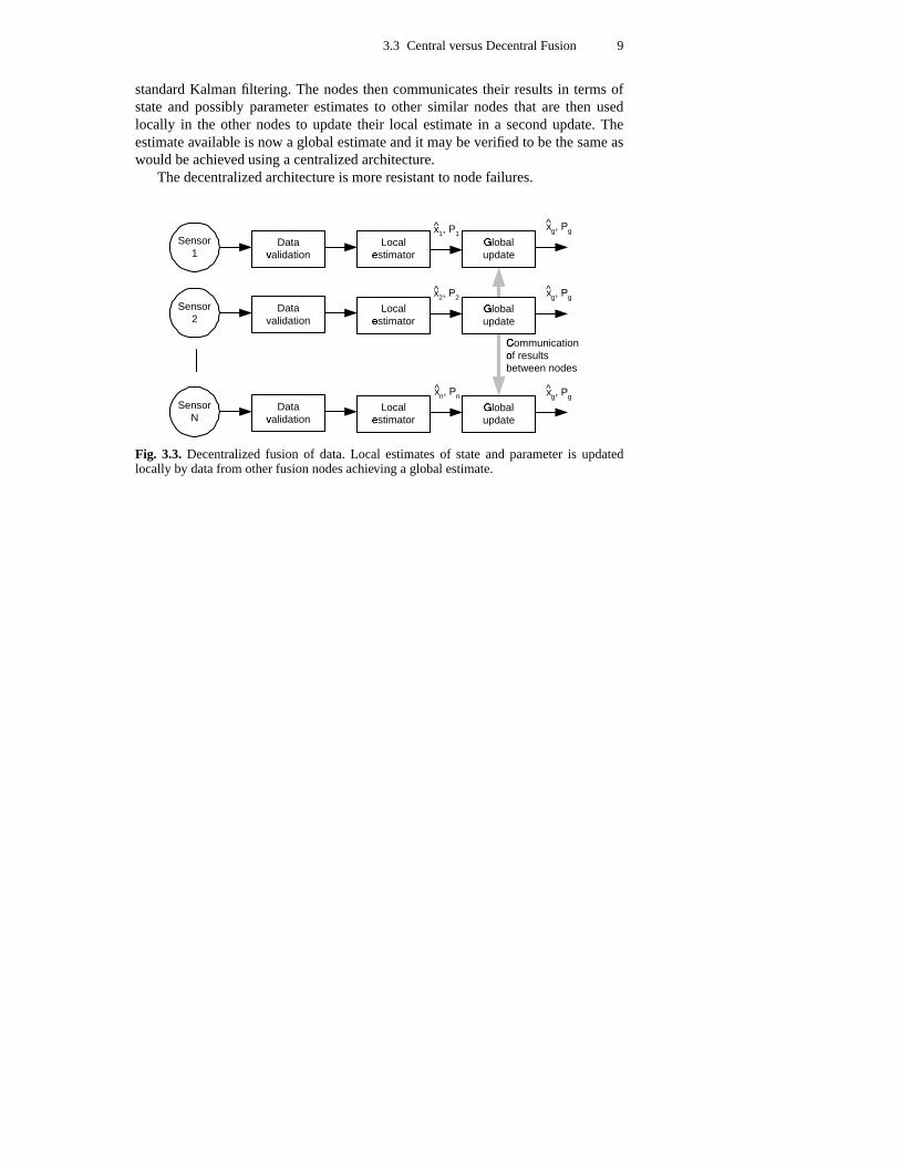
standardKalmanfiltering. The nodesthencommunicatestheir resultsin termsofstateand possiblyparameterestimatesto other similar nodesthat are then usedlocally in the other nodesto updatetheir local estimatein a secondupdate.Theestimateavailableis now a globalestimateandit maybeverifiedto bethesameaswould beachievedusinga centralizedarchitecture.

Thedecentralizedarchitectureis moreresistantto nodefailures.

Sensor 1

Sensor 2

Sensor N

Data validation �

Data validation

Data validation �

Local estimator �

Local estimator �

Local estimator �

Global update

x g , P g ^

Global update

x 2 , P 2

Global update

x n , P n

^

^

Communication of results �between nodes

x g , P g ^

x g , P g ^

x 1 , P 1 ^

Fig. 3.3. Decentralizedfusion of data.Local estimatesof stateand parameteris updatedlocally by datafrom otherfusionnodesachieving a globalestimate.

10 4. Multiple Model Estimation

4. Multiple Model Estimation

This chapterextendsthe considerationof estimationtheoryto considerthe useofmultiple processmodels.Multiple processmodelsoffer a numberof importantad-vantagesoversinglemodelestimators.

Multiple modelsallow a modularapproachto be taken. Ratherthan developa singlemodelwhich mustbe accuratefor all possibletypesof behaviour by thetruesystem,a numberof differentmodelscanbederived.Eachmodelhasits ownpropertiesand,with anappropriatechoiceof a datafusionalgorithm,it is possibleto spana largermodelspace.

Four different strategies for multiple model estimationare examinedin thischapter

– multiple modelswitching– multiple modeldetection– multiple hypothesistesting– multiple modelfusion

Although the detailsof eachschemeis different,the threefirst all usefunda-mentallythe sameapproach.The designerspecifiesa setof models.At any giventime only oneof thesemodelsis correctandall theothermodelsareincorrect. Thedifferentstrategiesusedifferenttypesof testto identify whichmodelis correctand,oncethis hasbeenachieved,theinformationfrom all theothermodelsis neglected.

The latterstrategy, modelfusionutilize thatprocessmodelsarea sourceof in-formationandtheir predictionscanbe viewed asthe measurementfrom a virtualsensor. Therefore,multiple model fusion can be cast in the sameframework asmultisensorfusion anda Kalmanupdaterule canbe usedto consistentlyfusethepredictionsof multiple processmodelstogether. This strategy hasmany importantbenefitsover the otherapproachesto multiple modelmanagement.It includestheability to exploit informationaboutthedifferencesin behaviour of eachmodel.Asa result,thefusionis synergistic: theperformanceof thefusedsystemcanbebetterthanthatof any individualmodel.

4.1 Benefitsof Multiple Models

Increasingthe complexity of a processmodeldoesnot necessarilyleadto a betterestimator. As the processmodel becomesmore complicated,it makes more and

4.1 Benefitsof Multiple Models 11

moreassumptionsaboutthe behaviour of the true system.Theseareembodiedasan increasingnumberof constraintson situationsin which the modelfits the realworld. Whenthe behaviour of the true systemis consistentwith the assumptionsin the model, its performanceis very good.However, when the behaviour is notconsistent,performancecanbesignificantlyworse.Simply increasingtheorderofthemodelwithout regardto this phenomenacouldleadto a very complicated,highorder model which works extremelywell in very limited circumstances.In mostothersituations,its performancecouldbepoor.

Multimodelestimationtechniquesareamethodwhichaddressesthisunderlyingproblem.Ratherthan seeka single model which is sufficiently complicatedandflexible thatit is consistentwith all possibletypesof behaviour for thetruesystem,anumberof low orderapproximatesystemsaredeveloped.Eachapproximatesystemis developedwith a differentassumptionsaboutthe behaviour of the true system.Sincetheseassumptionsare different, the situationsin which eachmodel fits isdifferent.

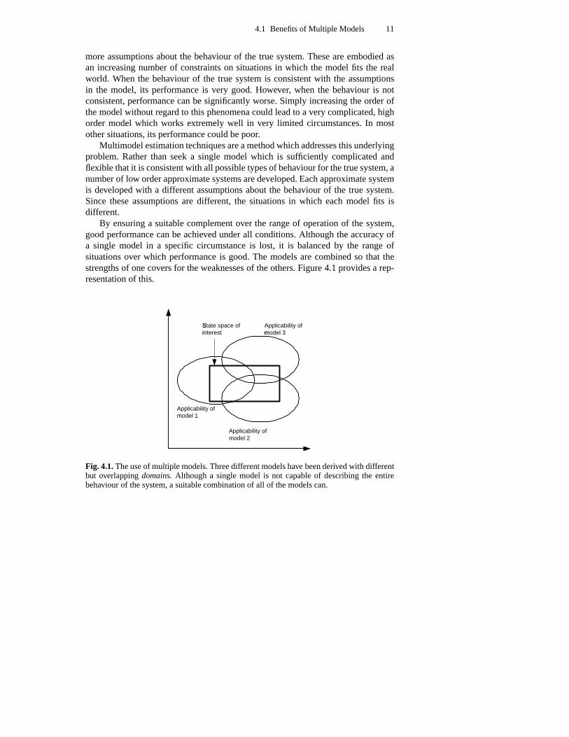
By ensuringa suitablecomplementover the rangeof operationof the system,goodperformancecanbe achievedunderall conditions.Although theaccuracy ofa single model in a specificcircumstanceis lost, it is balancedby the rangeofsituationsover which performanceis good.The modelsarecombinedso that thestrengthsof onecoversfor theweaknessesof theothers.Figure4.1providesa rep-resentationof this.

Applicability of model 3 �

Applicability of model 2

Applicability of model 1

State space of interest �

Fig. 4.1.Theuseof multiplemodels.Threedifferentmodelshavebeenderivedwith differentbut overlappingdomains. Although a singlemodel is not capableof describingthe entirebehaviour of thesystem,a suitablecombinationof all of themodelscan.


4.2 Problem Formulation

Supposea setof � processmodelshave beenderived.Eachusesa differentsetofassumptionsaboutthetruesystem,andtheresultis asetof � approximatesystems.The i’ th approximatesystemis describedusingtheprocessandobservationmodels�� "!$#%�'&)(+*%,.-/�.0213��4!$#%� (4.1)56�)��78��9�)��'&)(+*��:0<;"� �� (4.2)

Thestatespaceof theapproximatesystemis relatedto thetruesystemstate,��= ,accordingto thestructuralequations� � ��9��?> � �� = ��'&)( * �

The problemis to find the estimateof the variablesof interest @ � �.A �� 1 withcovarianceBDCEC ��.A �� whichtakesaccountof all of thedifferentapproximatemodelssuchthat the traceof BDCEC � �.A �9� is minimized.The strategy is not limited to justcombiningthe estimatesof the variablesin anoutputstage,the estimatemayalsobefeedbackto eachof theapproximatesystems,directly affectingtheir estimates.

This is reflectedin themodelmanagementstrategy which maybesummarizedin termsof two setsof functions– thecritical valueoutputfunction@ ��GFH� @ -��'& �/�I� & @�J � ��K� (4.3)

which combinethe multiple modelestimatesand the approximatesystemupdatefunction � � ��9�� - � ��& �/�/� &�� J � ��K� (4.4)

that updatesthe L ’ th model state.A successfulmultimodel managementstrategyshouldhavethefollowing properties:

Consistency. Theestimateshouldalwaysbeconsistent2. Theestimatesbecomein-consistentwhenthediscrepancy betweentheestimatedcovarianceandthetruecovarianceis not positivesemidefinite.

Performance. Thereshouldbe a performanceadvantageover usinga singlepro-cessmodel.This justifiestheextra complexity of usingmultimodelsinsteadofasinglemodel.Thesebenefitsincludemoreaccurateestimatesandmorerobustsolutions.

Theory. Themethodshouldhave a firm theoreticalfoundation.Not only doesthismeanthattherangeof applicabilityis known,but it isalsopossibleto generalizethetechniqueto a wide rangeof applications.M

Thewholestatespacemaynotbeof interest,and N9OQP9R PTS maythusbeasubsetof U3OQP9R PTSVThat is WXOZYKR [�S3\^]�_aÙcbdYKR [�S/Ùae b YKR [�S)R f�g�hjiHk where Ù arestateerrors,and f�g aremeasure-mentsup to time lmg

4.3 Methodsof Multi-Model Estimation 13

4.3 Methods of Multi-Model Estimation

Theprincipleandpracticeof multiple modelestimationhasbeenusedextensivelyfor many years.Thissectionreviewsvariousmultimodelschemes.

4.3.1 Model Switching Methods

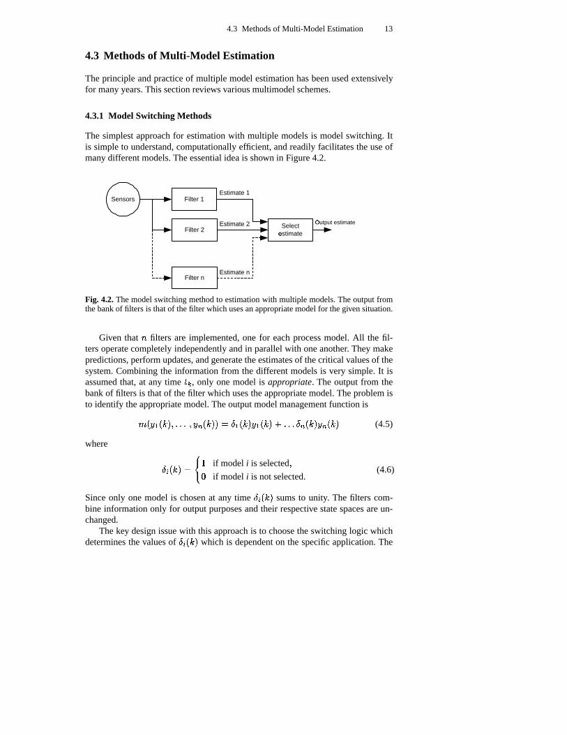
The simplestapproachfor estimationwith multiple modelsis modelswitching.Itis simpleto understand,computationallyefficient,andreadily facilitatestheuseofmany differentmodels.Theessentialideais shown in Figure4.2.

Sensors Filter 1

Filter 2 Select

estimate nEstimate 1

Filter n

Output estimate o

Estimate 2

Estimate n

Fig. 4.2.Themodelswitchingmethodto estimationwith multiple models.Theoutputfromthebankof filters is thatof thefilter whichusesanappropriatemodelfor thegivensituation.

Given that � filters are implemented,one for eachprocessmodel.All the fil-tersoperatecompletelyindependentlyandin parallelwith oneanother. They makepredictions,performupdates,andgeneratetheestimatesof thecritical valuesof thesystem.Combiningthe informationfrom the differentmodelsis very simple.It isassumedthat,at any time ( * , only onemodel is appropriate. The outputfrom thebankof filters is thatof thefilter which usestheappropriatemodel.Theproblemisto identify theappropriatemodel.TheoutputmodelmanagementfunctionisFp� @ - ��'& �/�I� & @ J � ��K�q�sr - ��9� @ - ��80 �/�I� r J �� @ J �� (4.5)

where r � ��9�� t # if modeli is selected&uif modeli is not selected.

(4.6)

Sinceonly onemodel is chosenat any time rI�� sumsto unity. The filters com-bine informationonly for outputpurposesandtheir respective statespacesareun-changed.

Thekey designissuewith this approachis to choosetheswitchinglogic whichdeterminesthevaluesof r � � �� which is dependenton thespecificapplication.The


landbasednavigationof theSpaceShuttle(Ewell 1988),for example,usestwo dif-ferent processmodelswhich correspondto acceleratingand cruising flight. Theacceleratingmodelis usedwhentheaccelerationexceedsa predefinedlimit. Whenaccelerationis below somecritical level, theshuttleis assumedto bein cruisemode.In thesecases,complex gravitationalandatmosphericmodelsareincorporatedintotheequationsof motion.Thethresholdwasselectedusingextensiveempiricaltests.

Switchingon thebasisof measurements(or estimates)may leadto jitter if theswitchingcriterion is noisy andits meanvalueis nearthe switchingthreshold.Amorerefinedsolutionis to employ hysteresisswitchingwhich switchesonly whenthereis a significantdifferencebetweentheperformanceof thedifferentmodels.

Althoughthemodelswitchingmethodandits variantsaresimpleto understandanduse,therearea significantnumberof problems.Themostimportantis that thechoiceof theswitchinglogic is oftenarbitrary, andhasto beselectedempirically–thereis no theoreticaljustificationthattheswitchinglogic is correct.

4.3.2 The Model DetectionMethod

Themodeldetectionapproachis a moresophisticatedversionof themodelswitch-ing method.Ratherthanswitchonthebasisof variousadhocthresholds,it attemptsto detectwhich model is the leastcomplex model(parsimonious((Ljung 1987))),which is capableof describingthemostsignificantfeaturesof thetruesystem.Theissueis a bias/variancetradeoff. As a modelbecomesmorecomplex, it becomesabetterdescriptionof the true system,andthe biasbecomesprogressively smaller.However, a morecomplex modelincludesmorestates.Giventhatthereis only afi-niteamountof noisydata,theresultis thattheinformationhasto bespreadbetweenthestatesandthevarianceon theestimatesof all of thestatesincrease.

For example,if a vehicleis driving in a straightline a very simplemodelmaybeused.However, whenthevehicleturn,theeffectsof dynamicsandslip mayhaveto beincluded.By ensuringthat theleastcomplex modelis usedat any givenpointin time, thevariancecomponentof thebias/variancetradeoff is minimizedso thatthemodelis not overly complicatedfor themaneuversin question.

Theoutputmodelmanagementfunction is of thesameform asEquations(4.5)and(4.6).No informationis propagatedfrom onemodelto thenext andtheapprox-imatesystemupdateis henceunity.

Onemethodfor testingwhethera modelis parsimoniousor not is to usemodelreductiontechniques.Theseexaminehow a high ordermodelcanbeapproximatedby a low ordermodel.A crucialcomponentfor any modelreductionschemeis theability to assessthe relative importancethatdifferentstateshave on the behaviourof thesystem.If a numberof stateshave very little effect on output,thenthey canbedeletedwithout introducingsubstantialerrors.

To make the contributionsfrom differentmodesclear, we turn to balancedre-alizations(Silvermann,Shookoohi, andDooren1983). In balancedrealizationsalinear transformationis appliedto the statespaceof the system.In this form, thecontribution of differentmodesis madeclear, anddecisionrulescanbeeasilyfor-mulated.


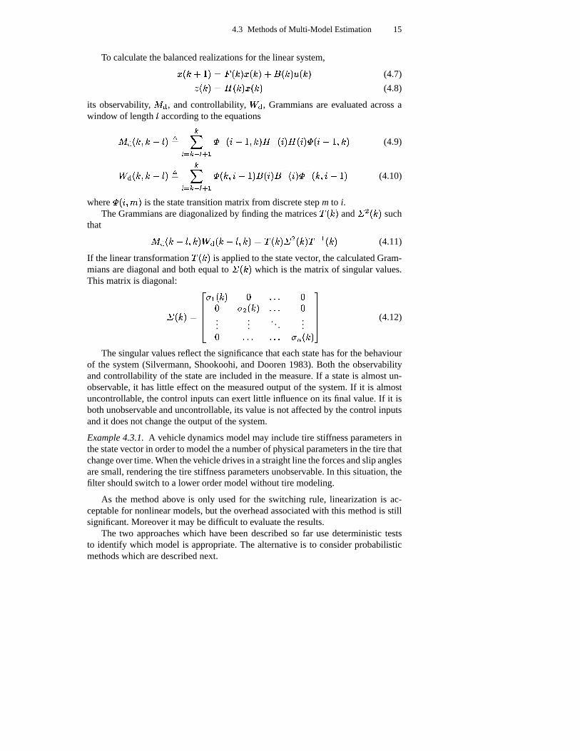
To calculatethebalancedrealizationsfor thelinearsystem,�:��v0s#%��xwy��K�8��9�:0{z|��9�~}�� (4.7)5c��x�2��K�8� �� (4.8)

its observability, �<� , andcontrollability, �� , Grammiansare evaluatedacrossawindow of length � accordingto theequations�<� ��3&��! � �� *��d�8*%,c��:-9�� L !$#�&��9�+� � � L �K�2� L � � � L !�#�&�� (4.9)

�� 3&��! � �� *��d�8*%,c��:-9� ��c& L !$#%�Kz|� L �Kz � � L � � � � �c& L !�#6� (4.10)

where � � L &�F�� is thestatetransitionmatrix from discretestepm to i.TheGrammiansarediagonalizedby finding thematrices� � �� and �"� ��9� such

that � � ��4! � &��9� � � ��! � &��9�� ,�- � �� (4.11)

If thelineartransformation� � �� is appliedto thestatevector, thecalculatedGram-miansarediagonalandbothequalto � �� which is thematrix of singularvalues.This matrix is diagonal:

� ��K� - �� u �/�I� uu� � � �� /�I� u

......

. . ....u �/�I� �/�I� � J � ��

�� (4.12)

Thesingularvaluesreflectthesignificancethateachstatehasfor thebehaviourof the system(Silvermann,Shookoohi, andDooren1983).Both the observabilityandcontrollability of thestateareincludedin themeasure.If a stateis almostun-observable,it haslittle effect on the measuredoutputof the system.If it is almostuncontrollable,thecontrol inputscanexert little influenceon its final value.If it isbothunobservableanduncontrollable,its valueis not affectedby thecontrolinputsandit doesnot changetheoutputof thesystem.

Example4.3.1. A vehicledynamicsmodelmayincludetire stiffnessparametersinthestatevectorin orderto modeltheanumberof physicalparametersin thetire thatchangeovertime.Whenthevehicledrivesin astraightline theforcesandslipanglesaresmall,renderingthetire stiffnessparametersunobservable.In this situation,thefilter shouldswitchto a lowerordermodelwithout tire modeling.

As the methodabove is only usedfor the switching rule, linearizationis ac-ceptablefor nonlinearmodels,but theoverheadassociatedwith this methodis stillsignificant.Moreover it maybedifficult to evaluatetheresults.

The two approacheswhich have beendescribedso far usedeterministicteststo identify which model is appropriate.The alternative is to considerprobabilisticmethodswhich aredescribednext.


4.3.3 Multiple HypothesisTesting

Multiple HypothesisTesting(Magill 1965)(MHT) is oneof themostwidely usedapproachesto multimodelestimation.Ratherthanusingboundsto defineregionsof applicability, eachmodelis consideredto bea candidatefor thetruemodel.Foreachmodel,thehypothesisthatit is thetruemodelis raised,andtheprobabilitythatthe hypothesisis correctis evaluatedusing the observation sequence.Over time,the mostaccuratemodel is assignedthe largestprobability andso dominatesthebehaviour of theestimator.

Figure4.3 shows the structureof this method.Eachmodel is implementedinits own filter andthe only interactionoccursin forming the output.The output isa functionof theestimatesmadeby thedifferentmodelsaswell astheprobabilitythat eachmodel is correct.The fusedestimateis not usedto refine the estimatesmaintainedin eachmodelandsotheapproximatesystemupdatefunctionsareunity.

Sensors Filter 1

Filter 2 Combine �estimates �

Filter n

Output estimate

Probablity calculation ¡

Fig. 4.3.Themodelhypothesismethod.Theoutputis afunctionof theestimatesmadeby thedifferentmodelsaswell astheprobabilitythateachmodelis correct.

Thefollowing two assumptionsaremade:

1. Thetruemodelis oneof thoseproposed.2. Thesamemodelhasbeenin actionsince (�� u

.

Fromthesetwo assumptions,asetof � hypothesesareformed,onefor eachmodel.Thehypothesisfor the L ’ th modelis�¢�8� Model � � is correct� (4.13)

By assumption1 thereis nonull hypothesisbecausethetruemodelis oneof modelsin the set.The probability thatmodel � � is correctat time ( * , conditionedon themeasurementsup to thattime, £ * is

4.3 Methodsof Multi-Model Estimation 17¤ � ��2¥:� � � A £ * � (4.14)

The initial probability that �H¦ is correct is given by ¤ ¦ � u � , which accordingtoassumption1 sumto unity overall models.

Theprobabilityassignedto eachmodelchangesthroughtime asmoreinforma-tion becomesavailable.Eachfilter predictsandupdatesaccordingto the Kalmanfilter equations.Considertheevolutionof ¤ ¦ from ��!�# to k. UsingBayes’rule¤ � ��§�<¥:� � � A £ * ��<¥:� � � A 5�� & £ *%,.- �� ¥:��5�� /A £ *%,.-%& � � �Q¥:� � ¦ A £ *%,�-I�¥:��5�� /A £ *6,�- �� ¥D��5c��IA £ *%,�- & � � �~¤ � ��!$#%�¨ J¦ �D- ¥:��5�� /A £ *6,�-%& � ¦ �Z¥D� � ¦ A £ *%,.-/� (4.15)

The ¥:��5�� /A £ *%,.- & � � � is the probability that theobservation 5c��9� would bemadegiventhat themodel �H¦ is valid. This probabilitymaybecalculateddirectly fromtheinnovations©'¦ � ��q��5c��!«ª5��.A �4!�#6� . Assumingthattheinnovationis Gaus-sian,zeromeanandhascovariance¬ ��8A ��!$#%� thelikelihoodis � �� #��®�¯8�+°²± �.³a´/µ � ¬ �� .A �4!$#%�� - ± � ´E¶a·c¸T¹�º (4.16)¸»¹�º �½¼�! #® © �� ¬ ,.-� � �.A �4!$#%� © � ��K¾ (4.17)

whereF is thedimensionof theinnovationvector.Theinnovationcovariance¬ �� is maintainedby theKalmanfilter andgivenby¬ � � �.A �"!$#%��x� � � �� B � ��K� �� 9�802¿ � �� (4.18)

The MHT now works by recursion,first calculate �)��9� for eachmodel.The

new probabilitiesarenow givenby¤.��q� �)��+¤.�� 4!�#6�¨ J¦ �:- ¦ ��+¤ ¦ ��!$#%� (4.19)

Theminimummeansquarederrorestimateis theexpectedvalue.Theoutputfunc-tion, i.e. theoutputof themultiplemodelis thusgivenbyª@ � �.A �9��GF?À @ - ��9��& �I�/� & @ J ��KÁ (4.20)�sÂ À @ ��IA £ * Á (4.21)�sÂÄÃ J� �d�:- @ �� Z¥D� � �)A £ *��~Å (4.22)� J� �d�:- ª@ � ¤ � � �� (4.23)


Thecovariancein theestimatecanbefoundto (Bar-ShalomandFortmann1988)BDCEC ��8A �� J� �d�:- ¤.�� À B ��Æ CEC � �.A �9�.0s�6ª@ �� .A ��!«ª@ � �.A �9�K�E�6ª@ ��.A ��D!Çª@ ��.A ��K� � Á(4.24)

which is a sumof probability weightedtermsfrom eachmodel.In additionto thedirectcovariancefrom themodels,a termis includedthattakesaccountfor thefactthat ª@ � is not equalto @ � .

TheMHT approachwasdevelopedinitially for problemsrelatedto systemiden-tification – the dynamicsof a nominal plant were specified,but therewas someuncertaintyin the valuesof several key parameters.A bankof filters wereimple-mented,one for eachfilter candidateparametervalue.Over time, onemodel ac-quiresa significantlygreaterprobability thantheothermodels,andit correspondsto themodelwhoseparametervaluesaremostappropriate.

The basicform of MHT hasbeenwidely employed in missile trackingwheredifferentmotion modelscorrespondto different typesof maneuvers(Bar-ShalomandFortmann1988).Experience,however, shows thattherearenumerouspracticalproblemswith applyingMHT. Theperformanceof thealgorithmis dependentupona significantdifferencebetweenthe residualcharacteristicsin the correct andthemismatchedfilters,which is sometimesdifficult to establish.

The threemethodswe have reviewed until now eachhasa numberof short-comings,many of which stemfrom the fact that they usefundamentallythe sameprinciple.Themethodsall at eachinstancein time assumedthatonly onemodeliscorrect, andthemultimodelfusionproblemis to identify thatmodel.However thisincludestheextremelystrongassumptionthatall theothermodels,no matterhowclosethey areto thecurrentmostappropriatemodel,provideno usefulinformationwhatever.

Theseshortcomingsmotivatethedevelopmentof anew strategy for fusinginfor-mationfrom multiple models.This approach,known asmodelfusion,is describednext.

4.3.4 Model Fusion

Themodelfusionapproachtreatseachprocessmodelasif it werea virtual sensor.The L ’ th processmodelis equivalentto asensorwhichmeasuresthepredictedvalueª�9�)��8A �Ä!s#%� . Themeasurementis corruptedby noise(thepredictionerror)andthesameprinciplesandtechniquesasin multi-sensorfusionmaybeused.

Figure4.4 illustratesthe methodfor two approximatesystems.Eachmodel isimplementedin its own filter and, in the predictionstep,eachfilter predictsthefuture stateof the system.Sinceeachfilter usesa differentmodelanda differentstatespace,thepredictionsaredifferent.

Filter 1 (or 2) propagatesits prediction(or somefunctionsof it) to filter 2 (or 1)which treatsit asif it wereanobservation.Eachfilter thenupdatesusingpredictionandsensorinformationalike.


Sensors È Filter 1

Filter 2

Batch estimator É Output estimate

ÊEstimate from filter 1

Estimate from filter 2

Prediction from filter 1 ËPrediction from filter 2 Ë

Fig. 4.4. Model fusion architecturefor two approximatesystems.Eachfilter predictsthefuture stateof thesystemusingthe sameinputs,andupdatesusingsensorinformationandthepredictionpropagatedfrom theotherfilter.

The processmodel is usedto predict the future stateof the system.Using theprocessmodelthepredictionsummarizesall thepreviousobservationinformation.Theestimateat (+* is thusnot restrictedto usingtheinformationcontainedin Ì �� .Thepredictionallow temporalfusionwith datafrom all pastmeasurements.

Thefusionof dataisbestappreciatedbyconsideringtheinformationform (May-beck1979)of theKalmanfilter prediction.Theamountof informationmaintainedinanestimateª� is definedto betheinverseof its covariancematrix.With theKalmangain Í , thecovariancepredictionmayberewrittenasB ��.A �� B ��.A �4!�#6�D! Í �2��9� B ��8A ��!$#%� (4.25)B � �.A �� B ,.- ��8A �4!$#%��«#²! Í �2�� (4.26)

Using this result in combinationwith the Kalman gain in termsof the predictedcovariance,(Maybeck1979)Í � B � �.A �9�+�2� �� ¿¢� �� ,.-

(4.27)

where ¿¢�� is themeasurementcovariance.Thestatemeasurementupdatemaybewrittenasª�D��.A �� B ��.A ��ÏÎ B ,.- ��8A �4!$#%��ª�8��8A ��!$#%�80{�2��9� � ¿¢��9� ,�- Ì ��~Ð (4.28)

A similarexpressioncanbefoundfor thepredictedinformationmatrixB � �.A �9� ,�- � B ��8A ��!$#%� ,.- 02�{�� ¿¢�� ,�- �2�� (4.29)

The estimatein Equation(4.28) is thereforea weightedaverageof the predic-tion andthe observation.Intuitively the weightsmustbe inverselyproportionaltotheir respective covariances.Seenin the light of Equation(4.28) predictionsandobservationsaretreatedequallyby theKalmanfilter. It is thereforepossibleto con-siderthepredictionfrom filter 1 (2) asanobservation, ª�:��.A �y!?#%� with covarianceB ,�- ��.A �4!$#%� thatcanbeusedto updatefilter 2 (1).


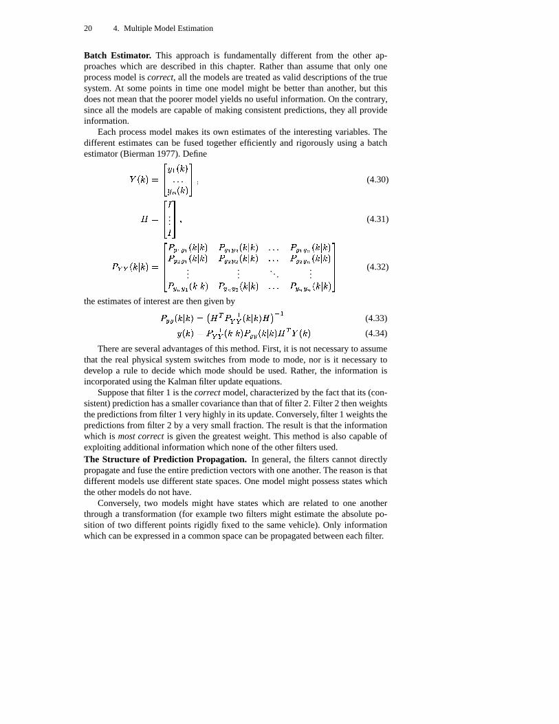
Batch Estimator. This approachis fundamentallydifferent from the other ap-proacheswhich are describedin this chapter. Ratherthan assumethat only oneprocessmodelis correct, all themodelsaretreatedasvalid descriptionsof thetruesystem.At somepoints in time onemodel might be betterthananother, but thisdoesnot meanthatthepoorermodelyieldsno usefulinformation.On thecontrary,sinceall the modelsarecapableof makingconsistentpredictions,they all provideinformation.

Eachprocessmodelmakesits own estimatesof the interestingvariables.Thedifferentestimatescanbe fusedtogetherefficiently and rigorously usinga batchestimator(Bierman1977).DefineÑ �� @ - � ��/�I�@ J ��9� �� & (4.30)

�Ò� ��KÓ ...Ó�� & (4.31)

B�Ô:Ô ��.A �� B CEÕKC'Õ ��.A �� B CEÕ+C)Ö ��.A �� /�I� B CEÕ+C�× ��8A ��B C�Ö)C'Õ ��.A �� B C�Ö�C)Ö ��.A �� /�I� B C�Ö�C�× ��8A ��...

.... . .

...B:C × C Õ � �.A �� B:C × C Ö � �.A �� /�I� B:C × C × ��8A �� (4.32)

theestimatesof interestarethengivenbyB C/C ��.A ��§� À �ÙØ B ,�-Ô�Ô ��.A ��K� Á ,.-(4.33)@ �� B ,�-Ô�Ô � �.A �� BDCEC � �.A �9�+�ÙØ Ñ ��9� (4.34)

Thereareseveraladvantagesof this method.First, it is not necessaryto assumethat the real physicalsystemswitchesfrom modeto mode,nor is it necessarytodevelop a rule to decidewhich modeshouldbe used.Rather, the information isincorporatedusingtheKalmanfilter updateequations.

Supposethatfilter 1 is thecorrectmodel,characterizedby thefactthatits (con-sistent)predictionhasasmallercovariancethanthatof filter 2. Filter 2 thenweightsthepredictionsfrom filter 1 veryhighly in its update.Conversely, filter 1 weightsthepredictionsfrom filter 2 by a very small fraction.Theresultis that theinformationwhich is mostcorrect is given the greatestweight.This methodis alsocapableofexploiting additionalinformationwhich noneof theotherfiltersused.The Structur e of Prediction Propagation. In general,the filters cannotdirectlypropagateandfusetheentirepredictionvectorswith oneanother. Thereasonis thatdifferentmodelsusedifferentstatespaces.Onemodelmight possessstateswhichtheothermodelsdonot have.

Conversely, two modelsmight have stateswhich are relatedto one anotherthrougha transformation(for exampletwo filters might estimatethe absolutepo-sition of two differentpointsrigidly fixed to the samevehicle).Only informationwhich canbeexpressedin a commonspacecanbepropagatedbetweeneachfilter.


A modeltranslatorfunction � -�Ú"- � �� - � ��K� propagatesthepredictionfrom filter1 into a statespacewhich is commonto bothfilters. Similarly, thepredictionfromfilter 2 is propagatedusing its own translatorfunction. The fusion spacefor bothfilters consistsof parameterswhich arethe samein both filters. Theseparametersobey theconditionthat � � Ú"- � �EÛ� � ��§� � -�Ú"- � �EÛ� - �� (4.35)

for all choicesof thetruestatespacevector �9=q��9� and Û�9�)��9�Ü�Ý>��K��=q� ��K� . Candi-datequantitiesinclude

– Stateswhich arecommonto bothmodels(suchasthepositionof thesamepointmeasuredin thesamecoordinatesystem).

– Thepredictedobservations.– Thepredictedvariables(statesof interest).

However, it is importantto stressthatmany statesdo not obey this condition.Thisis becausemany statesare lumpedparameters:their valuereflectsthe net effectsof many differentphysicalprocesses.Sincedifferentapproximatesystemsusedif-ferent assumptions,different physicalprocessesare lumpedtogetherin differentparameters.

Eachfilter treatsthe propagationfrom the otherfilter asa type of observationwhich is appendedto theobservationstatespace.Therefore,theobservationvectorwhich is receivedby filter 1 is5�-Þ��9��àß 5c��9�� Ú�- � �� 9�K�~á (4.36)

The model fusion is a straightforward procedure.For eachpair of modelsfind acommonstatespacein whichtheconditionof Equation(4.35)hold.Theobservationspacefor eachfilter is augmentedappropriately, and the applicationof the filterfollows trivially.

Themodelfusionsystemrelieson theKalmanfilter for its informationpropa-gation,andwe will hencehave to take accountof that the predictionerrorsin thedifferentmodelsarecorrelatedwith oneanotherin orderto getconsistentestimates.

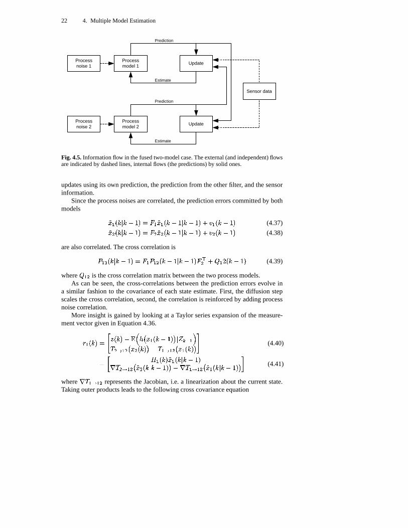
Figure4.5showstheinformationflowswhichoccurwhentwo modelsarefused.Informationcanbeclassifiedin two forms: informationwhich flows from theout-side(andis independent)andthatwhich flows within (thepredictionswhich prop-agatebetweenthefilters).Theexternalflowsareindicatedby dashedlines,internalflows by solid ones.Both flows play a key role in thepredictionandtheupdate.Inthepredictionstepeachfilter usesits own processmodelto estimatethefuturestateof thesystem.

Theprocessnoisesexperiencedby eachmodelarenot independentfor two rea-sons.First, thereis a componentdueto the truesystemprocessnoise.Second,themodelingerrortermsfor eachfilter areevaluatedaboutthetruesystemstate.Sincetheprocessnoisesarecorrelated,thepredictionerrorsarealsocorrelated.Eachfilter


Sensor data

Process model 1

Update

Prediction

Estimate

Process noise 1

Process model 2

Update

Prediction

Estimate

Process noise 2

Fig. 4.5.Informationflow in thefusedtwo-modelcase.Theexternal(andindependent)flowsareindicatedby dashedlines,internalflows (thepredictions)by solid ones.

updatesusingits own prediction,thepredictionfrom theotherfilter, andthesensorinformation.

Sincetheprocessnoisesarecorrelated,thepredictionerrorscommittedby bothmodels â� - � �.A �"!$#%��xw - â� - ��4!$#»A �"!�#6�80<1 - ��4!$#%� (4.37)

â� � � �.A �"!$#%��xw � â� � ��4!$#»A �"!�#6�80<1 � ��4!$#%� (4.38)

arealsocorrelated.ThecrosscorrelationisB - � ��.A ��!�#6��sw - B - � ��4!$#»A �"!�#6�+w �� 0�ã - ®9��!�#6� (4.39)

where ã - � is thecrosscorrelationmatrixbetweenthetwo processmodels.As canbe seen,the cross-correlationsbetweenthe predictionerrorsevolve in

a similar fashionto the covarianceof eachstateestimate.First, the diffusion stepscalesthecrosscorrelation,second,thecorrelationis reinforcedby addingprocessnoisecorrelation.

More insight is gainedby looking at a Taylor seriesexpansionof themeasure-mentvectorgivenin Equation4.36.© -��åä 5c��D!pÂ�¼67 À �3-�� "!$#%� Á A £ *6,�-/¾� � Ú"- � À � � �� Á ! � -KÚ"- � À �c-��9� ÁEæ (4.40)�çß � - �� â� - ��.A �4!$#%�è � � Ú"- � À â� � ��.A ��!�#6� Á ! è � -KÚ�- � À â� - � �.A ��!$#%� Á á (4.41)

whereè � -�Ú"- � representstheJacobian,i.e. a linearizationaboutthe currentstate.

Takingouterproductsleadsto thefollowing crosscovarianceequation

4.3 Methodsof Multi-Model Estimation 23BDé ÕKê�Õ � �.A �"!$#%��çß B -)-Þ��8A �4!$#%�K� Ø- � ��B -)-Þ� �.A �4!�#6� è � � -KÚ�- � ! B - � ��.A �4!�#6� è � � � Ú"- � á (4.42)

whichshowshow informationflowsbetweenthetwo filters.Thefirst componentde-scribeshow theobservationinformationis injected.Thesecondcomponent,whichdeterminedtheweightplacedon thepredictionpropagatedfrom filter 2, is thedif-ferencebetweenthecovarianceof filter 1, andthecrosscorrelationbetweenfilters1and2 all projectedinto thesamespace.

In effect only the informationwhich is uniqueto filter 2 is propagatedto filter1. As the two filters becomemoreandmoresimilar to oneanother, they becomemoreandmoretightly correlated.Lessinformationis propagatedfrom filter 2 and,in the limit whenbothfilters useexactly thesameprocessmodels,no informationis passedbetweenthemat all. Model fusion doesnot invent informationover andabovewhatcanbeobtainedfrom thesensors.Rather, it is a differentway to exploitthe observations.In the otherlimit, asthe modelsbecomelessandlesscorrelatedwith oneanother, the predictionscontainmoreandmoreindependentinformationandso is assigneda progressively greaterweight. The updateenforcesthe corre-lation betweenthe filters throughthe fact that the sameobservationsareusedtoupdatebothfilters with thesameobservationnoises.

Therathercomplex crosscorrelationsin theobservationnoisemaybesimplifiedby treatingthe network of filters andcrosscorrelationfilters ascomponentsof asingle,all encompassingsystemor combinedsystem.

4.3.5 Combined System

The combinedsystemis formedby stackingthe statespacesof eachapproximatesystem.Thecombinedstatespacevector ��ë is

�9ëÞ��9�� - �� ...�cì��

�� (4.43)

The dimensionof � ë is the sum of the dimensionsof the subsystemfilters. Thecovarianceof thecombinedsystemis

B ë6��.A �� B -)- � �.A �9� B - � ��8A �� ¹I¹/¹ B - J � �.A �9�B � - � �.A �9� B �� 8A �� ¹I¹/¹ B � J � �.A �9�...

.... . .

...B:J -��8A �� BDJ � ��.A �� ¹I¹/¹ BDJ�J ��.A �� (4.44)

Thediagonalsubblocksarethecovariancesof thesubsystems,andtheoff diagonalsubblocksarethecorrelationsbetweenthem.

Thecombinedsystemevolvesover time accordingto a processmodelwhich iscorruptedby processnoise.Thesearegivenby stackingthecomponentsfrom eachsubsystem:


� ë �� ë ��.A ��&)}D� ��&)1 ë ��'&)( * �§� �� - �� - � ��&)}D� ��&)1 - � ��&�( * �� &)}D� ��&)1 � � ��&�( * �...� J �� J ��9��&�}��9��&�1 J ��'&)( * �

� �� (4.45)

Theassociatedcovarianceis

ã ë � ��§�åíîîîîïã -)- ��9�ðã - � � �� ¹/¹I¹ ã - J � ��ã � - ��9�ðã �)� � �� ¹/¹I¹ ã � J � ��

......

. . ....ã J - ��ñã J � � �� . . . ã J�J ��9�

òEóóóóô (4.46)

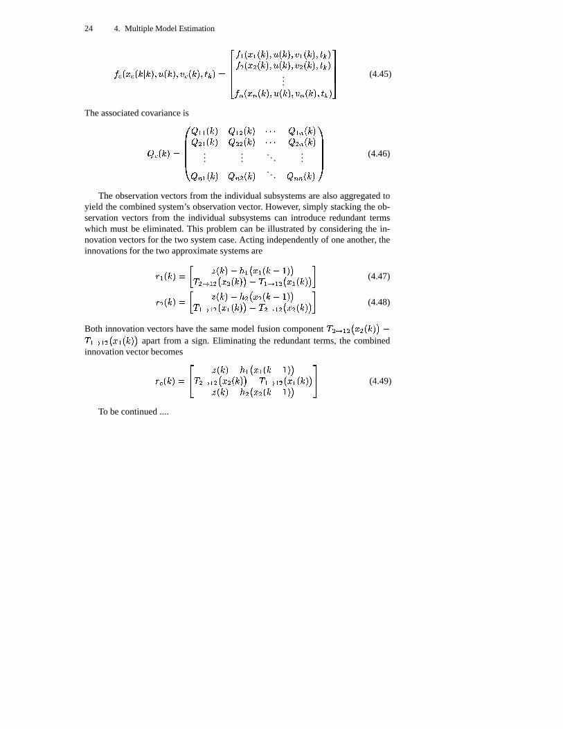
Theobservationvectorsfrom the individual subsystemsarealsoaggregatedtoyield thecombinedsystem’s observationvector. However, simply stackingtheob-servation vectorsfrom the individual subsystemscan introduceredundanttermswhich mustbe eliminated.This problemcanbe illustratedby consideringthe in-novationvectorsfor thetwo systemcase.Acting independentlyof oneanother, theinnovationsfor thetwo approximatesystemsare© - ��§� ß 5c��9�D!p7 - À � - ��4!$#%�+Á� � Ú"- � À � � �� Á ! � -KÚ"- � À � - ��9� Á á (4.47)© � ��§� ß 5c��9�D!p7 � À � � ��4!$#%� Á� -�Ú"- � À � - �� Á ! � � Ú"- � À � � ��9� Á á (4.48)

Both innovationvectorshave thesamemodelfusioncomponent� � Ú"- � À � � �� Á !� -KÚ�- � À � - � �� Á apartfrom a sign. Eliminating the redundantterms,the combinedinnovationvectorbecomes© ë%� �� 5c��9�D!p73- À �c-��!$#%� Á� � Ú"- � À � � �� Á ! � -KÚ"- � À �c-��9� Á5c��9�D!p7 � À � � ��!$#%� Á �� (4.49)

To becontinued....

REFERENCES 25

References

Bar-Shalom,Y. andT. E. Fortmann(1988).Tracking andData Assocations. TheAcademicPress.

Bierman,G.J.(1977).FactorizationMethodsfor DiscreteSequentialEstimation,Volume128of Mathematicsin ScienceandEngineering. AcademicPress.

Ewell, J. J. (1988).Spaceshuttleorbiterentry throughlandnavigation.In IEEEInternationalConferenceon IntelligentRobotsandSystems, pp.627–632.

Ljung, L. (1987).SystemIdentification,Theoryfor theUser. Prentice-Hallinfor-mationandsystemsciencesseries.Prentice-Hall.

Magill, D. D. (1965,October).Optimaladaptiveestimationof sampledstochasticprocesses.IEEE transactiononautomaticControl 10(4), 434–439.

Maybeck,P. S. (1979).StochasticModels,Estimation,and Control, Volume1.AcademicPress.

Silvermann,L., S. Shookoohi, andP. V. Dooren(1983,August).Linear time-variablesystems:Balancingandmodelreduction.IEEEtransactiononauto-maticControl 28(8), 810–822.

Sensfusion

Education

Transcript of Sensfusion