Semidefinite Optimization - Institut de Math©matiques de Bordeaux

Semidefinite Optimization

MastermathSpring 2012

Monique Laurent

Centrum Wiskunde & Informatica

Science Park 123

1098 XG Amsterdam

The Netherlands

[email protected]

Frank Vallentin

Delft Institute of Applied Mathematics

Technical University of Delft

P.O. Box 5031

2600 GA Delft

The Netherlands

[email protected]

May 22, 2012

CONTENTS

I Theory and algorithms for semidefinite optimization 1

1 Background: Convex sets and positive semidefinite matrices 21.1 Some fundamental notions . . . . . . . . . . . . . . . . . . . . . 3

1.1.1 Euclidean space . . . . . . . . . . . . . . . . . . . . . . . . 31.1.2 Topology in finite-dimensional metric spaces . . . . . . . . 31.1.3 Affine geometry . . . . . . . . . . . . . . . . . . . . . . . . 4

1.2 Convex sets . . . . . . . . . . . . . . . . . . . . . . . . . . . . . . 51.3 Implicit description of convex sets . . . . . . . . . . . . . . . . . . 6

1.3.1 Metric projection . . . . . . . . . . . . . . . . . . . . . . . 71.3.2 Separating and supporting hyperplanes . . . . . . . . . . 9

1.4 Explicit description of convex sets . . . . . . . . . . . . . . . . . . 121.5 Convex cones . . . . . . . . . . . . . . . . . . . . . . . . . . . . . 131.6 Examples . . . . . . . . . . . . . . . . . . . . . . . . . . . . . . . 14

1.6.1 The non-negative orthant and linear programming . . . . 151.6.2 The second-order cone . . . . . . . . . . . . . . . . . . . . 151.6.3 The cone of semidefinite matrices . . . . . . . . . . . . . . 151.6.4 The copositive cone . . . . . . . . . . . . . . . . . . . . . 16

1.7 Positive semidefinite matrices . . . . . . . . . . . . . . . . . . . . 161.7.1 Basic facts . . . . . . . . . . . . . . . . . . . . . . . . . . . 161.7.2 The trace inner product . . . . . . . . . . . . . . . . . . . 171.7.3 Hoffman-Wielandt inequality . . . . . . . . . . . . . . . . 181.7.4 Schur complements . . . . . . . . . . . . . . . . . . . . . 191.7.5 Block-diagonal matrices . . . . . . . . . . . . . . . . . . . 201.7.6 Kronecker and Hadamard products . . . . . . . . . . . . . 21

1.8 Historical remarks . . . . . . . . . . . . . . . . . . . . . . . . . . 211.9 Further reading . . . . . . . . . . . . . . . . . . . . . . . . . . . . 231.10 Exercises . . . . . . . . . . . . . . . . . . . . . . . . . . . . . . . . 23

i

2 Semidefinite programs: Basic facts and examples 262.1 Primal and dual semidefinite programs . . . . . . . . . . . . . . . 27

2.1.1 Primal form . . . . . . . . . . . . . . . . . . . . . . . . . . 272.1.2 Dual form . . . . . . . . . . . . . . . . . . . . . . . . . . . 28

2.2 Eigenvalue optimization . . . . . . . . . . . . . . . . . . . . . . . 292.3 Convex quadratic constraints . . . . . . . . . . . . . . . . . . . . 322.4 Robust optimization . . . . . . . . . . . . . . . . . . . . . . . . . 332.5 Examples in combinatorial optimization . . . . . . . . . . . . . . 35

2.5.1 The maximum independent set problem . . . . . . . . . . 352.5.2 The maximum cut problem . . . . . . . . . . . . . . . . . 36

2.6 Examples in geometry . . . . . . . . . . . . . . . . . . . . . . . . 372.7 Examples in algebra . . . . . . . . . . . . . . . . . . . . . . . . . 382.8 Further reading . . . . . . . . . . . . . . . . . . . . . . . . . . . . 392.9 Exercises . . . . . . . . . . . . . . . . . . . . . . . . . . . . . . . . 40

3 Duality in conic programming 433.1 Fundamental properties . . . . . . . . . . . . . . . . . . . . . . . 45

3.1.1 Local minimizers are global minimizers . . . . . . . . . . 453.1.2 Karush-Kuhn-Tucker condition . . . . . . . . . . . . . . . . 45

3.2 Primal and dual conic programs . . . . . . . . . . . . . . . . . . . 463.2.1 Primal conic programs . . . . . . . . . . . . . . . . . . . . 463.2.2 Dual conic programs . . . . . . . . . . . . . . . . . . . . . 463.2.3 Geometric interpretation of the primal-dual pair . . . . . . 47

3.3 Examples . . . . . . . . . . . . . . . . . . . . . . . . . . . . . . . 483.3.1 Linear programming (LP) . . . . . . . . . . . . . . . . . . 483.3.2 Conic quadratic programming (CQP) . . . . . . . . . . . . 493.3.3 Semidefinite programming (SDP) . . . . . . . . . . . . . . 49

3.4 Duality theory . . . . . . . . . . . . . . . . . . . . . . . . . . . . . 503.5 Some pathological examples . . . . . . . . . . . . . . . . . . . . . 53

3.5.1 Dual infimum not attained . . . . . . . . . . . . . . . . . . 533.5.2 Positive duality gap . . . . . . . . . . . . . . . . . . . . . . 53

3.6 Strong and weak infeasibility . . . . . . . . . . . . . . . . . . . . 543.7 More on the difference between linear and conic programming . 573.8 Further reading . . . . . . . . . . . . . . . . . . . . . . . . . . . . 573.9 Historical remarks . . . . . . . . . . . . . . . . . . . . . . . . . . 583.10 Exercises . . . . . . . . . . . . . . . . . . . . . . . . . . . . . . . . 58

4 Interior point methods 614.1 Classical barrier methods . . . . . . . . . . . . . . . . . . . . . . 62

4.1.1 Newton’s method . . . . . . . . . . . . . . . . . . . . . . . 624.1.2 Barrier method . . . . . . . . . . . . . . . . . . . . . . . . 664.1.3 Finding a starting point . . . . . . . . . . . . . . . . . . . 67

4.2 Central path of a semidefinite program . . . . . . . . . . . . . . . 684.3 Software . . . . . . . . . . . . . . . . . . . . . . . . . . . . . . . . 704.4 Historical remarks . . . . . . . . . . . . . . . . . . . . . . . . . . 714.5 Further reading . . . . . . . . . . . . . . . . . . . . . . . . . . . . 72

ii

II Applications in combinatorics 75

5 01 optimization 765.1 Relaxations using quadratic optimization . . . . . . . . . . . . . . 775.2 A hierarchy of semidefinite programs . . . . . . . . . . . . . . . . 80

5.2.1 Harmonic analysis on power sets . . . . . . . . . . . . . . 815.2.2 Lasserre’s hierarchy . . . . . . . . . . . . . . . . . . . . . 845.2.3 Example: Independence number . . . . . . . . . . . . . . 88

5.3 Further reading . . . . . . . . . . . . . . . . . . . . . . . . . . . . 895.4 Exercises . . . . . . . . . . . . . . . . . . . . . . . . . . . . . . . . 90

6 Graph coloring and independent sets 926.1 Preliminaries on graphs . . . . . . . . . . . . . . . . . . . . . . . 92

6.1.1 Stability and chromatic numbers . . . . . . . . . . . . . . 926.1.2 Perfect graphs . . . . . . . . . . . . . . . . . . . . . . . . . 93

6.2 Linear programming bounds . . . . . . . . . . . . . . . . . . . . . 946.3 Semidefinite programming bounds . . . . . . . . . . . . . . . . . 96

6.3.1 The theta number . . . . . . . . . . . . . . . . . . . . . . 966.3.2 Computing maximum stable sets in perfect graphs . . . . 976.3.3 Minimum colorings of perfect graphs . . . . . . . . . . . . 98

6.4 Other formulations of the theta number . . . . . . . . . . . . . . 996.4.1 Dual formulation . . . . . . . . . . . . . . . . . . . . . . . 996.4.2 Two more (lifted) formulations . . . . . . . . . . . . . . . 100

6.5 Geometric properties of the theta number . . . . . . . . . . . . . 1016.5.1 Orthonormal representations . . . . . . . . . . . . . . . . 1016.5.2 The theta body THpGq . . . . . . . . . . . . . . . . . . . . 1026.5.3 More on the theta body . . . . . . . . . . . . . . . . . . . 103

6.6 The theta number for vertex-transitive graphs . . . . . . . . . . . 1046.7 Bounding the Shannon capacity . . . . . . . . . . . . . . . . . . . 1066.8 Further reading . . . . . . . . . . . . . . . . . . . . . . . . . . . . 1086.9 Exercises . . . . . . . . . . . . . . . . . . . . . . . . . . . . . . . . 108

7 Approximating MAX CUT and the cut norm 1117.1 The algorithm of Goemans and Williamson . . . . . . . . . . . . . 112

7.1.1 Semidefinite relaxation . . . . . . . . . . . . . . . . . . . 1127.1.2 Analysis of the algorithm . . . . . . . . . . . . . . . . . . 1147.1.3 Remarks on the algorithm . . . . . . . . . . . . . . . . . . 117

7.2 Cut norm and Grothendieck’s inequality . . . . . . . . . . . . . . 1177.2.1 Cut norm of a matrix . . . . . . . . . . . . . . . . . . . . . 1177.2.2 Grothendieck’s inequality . . . . . . . . . . . . . . . . . . 1197.2.3 Proof of Grothendieck’s inequality . . . . . . . . . . . . . 120

7.3 Further reading . . . . . . . . . . . . . . . . . . . . . . . . . . . . 1227.4 Historical remarks and anecdotes . . . . . . . . . . . . . . . . . . 1227.5 Questions . . . . . . . . . . . . . . . . . . . . . . . . . . . . . . . 123

iii

8 Generalizations of Grothendieck’s inequality and applications 1268.1 The Grothendieck constant of a graph . . . . . . . . . . . . . . . 128

8.1.1 Randomized rounding by truncating . . . . . . . . . . . . 1298.1.2 Quality of expected solution . . . . . . . . . . . . . . . . . 1308.1.3 A useful lemma . . . . . . . . . . . . . . . . . . . . . . . . 1308.1.4 Estimating A and B in the useful lemma . . . . . . . . . . 1318.1.5 Applying the useful lemma . . . . . . . . . . . . . . . . . 1328.1.6 Connection to the theta number . . . . . . . . . . . . . . . 132

8.2 Higher rank Grothendieck inequality . . . . . . . . . . . . . . . . 1338.2.1 Randomized rounding by projecting . . . . . . . . . . . . 1348.2.2 Extension of Grothendieck’s identity . . . . . . . . . . . . 1348.2.3 Proof of the theorem . . . . . . . . . . . . . . . . . . . . . 135


III Applications in geometry 138

9 Optimizing with ellipsoids and determinants 1399.1 Determinant maximization problems . . . . . . . . . . . . . . . . 1409.2 Convex spectral functions . . . . . . . . . . . . . . . . . . . . . . 141

9.2.1 Minkowski’s determinant inequality . . . . . . . . . . . . 1429.2.2 Davis’ characterization of convex spectral functions . . . . 142

9.3 Approximating polytopes by ellipsoids . . . . . . . . . . . . . . . 1459.3.1 Inner approximation . . . . . . . . . . . . . . . . . . . . . 1459.3.2 Outer approximation . . . . . . . . . . . . . . . . . . . . . 146

9.4 The Lowner-John ellipsoids . . . . . . . . . . . . . . . . . . . . . 1479.5 Further reading . . . . . . . . . . . . . . . . . . . . . . . . . . . . 1519.6 Exercises . . . . . . . . . . . . . . . . . . . . . . . . . . . . . . . . 151

10 Euclidean embeddings: Low dimension 15410.1 Geometry of the positive semidefinite cone . . . . . . . . . . . . . 155

10.1.1 Faces of convex sets . . . . . . . . . . . . . . . . . . . . . 15510.1.2 Faces of the positive semidefinite cone . . . . . . . . . . . 15610.1.3 Faces of spectrahedra . . . . . . . . . . . . . . . . . . . . 15710.1.4 Finding an extreme point in a spectrahedron . . . . . . . . 16010.1.5 A refined bound on ranks of extreme points . . . . . . . . 160

10.2 Applications . . . . . . . . . . . . . . . . . . . . . . . . . . . . . . 16210.2.1 Euclidean realizations of graphs . . . . . . . . . . . . . . . 16210.2.2 Hidden convexity results for quadratic maps . . . . . . . . 16410.2.3 The S-Lemma . . . . . . . . . . . . . . . . . . . . . . . . . 166

10.3 Notes and further reading . . . . . . . . . . . . . . . . . . . . . . 16710.4 Exercises . . . . . . . . . . . . . . . . . . . . . . . . . . . . . . . . 168

iv

11 Euclidean embeddings: Low distortion 17111.1 Motivation: Embeddings of finite metric spaces . . . . . . . . . . 17111.2 Computing optimal Euclidean embeddings . . . . . . . . . . . . . 173

11.2.1 Least distortion embedding of the cube . . . . . . . . . . . 17411.3 Corner stones of metric embeddings . . . . . . . . . . . . . . . . 174

11.3.1 Bourgain’s theorem . . . . . . . . . . . . . . . . . . . . . . 17411.3.2 Johnson-Lindenstrauss flattening lemma . . . . . . . . . . 175

11.4 Embeddings of expanders . . . . . . . . . . . . . . . . . . . . . . 17511.4.1 Edge expansion . . . . . . . . . . . . . . . . . . . . . . . . 17511.4.2 Large spectral gap implies high expansion . . . . . . . . . 17611.4.3 High expansion implies large spectral gap . . . . . . . . . 17711.4.4 Low distortion embeddings of expander graphs . . . . . . 17911.4.5 Construction of a family of expander graphs . . . . . . . . 181


12 Packings on the sphere 18412.1 α and ϑ for packing graphs . . . . . . . . . . . . . . . . . . . . . 18512.2 Symmetry reduction . . . . . . . . . . . . . . . . . . . . . . . . . 18712.3 Schoenberg’s theorem . . . . . . . . . . . . . . . . . . . . . . . . 18812.4 Proof of Schoenberg’s theorem . . . . . . . . . . . . . . . . . . . 190

12.4.1 Orthogonality relation . . . . . . . . . . . . . . . . . . . . 19012.4.2 Positive semidefiniteness . . . . . . . . . . . . . . . . . . . 19012.4.3 End of proof . . . . . . . . . . . . . . . . . . . . . . . . . 191

12.5 Delsarte’s LP method . . . . . . . . . . . . . . . . . . . . . . . . . 19312.6 τ8 equals 240 . . . . . . . . . . . . . . . . . . . . . . . . . . . . . 19412.7 Further reading . . . . . . . . . . . . . . . . . . . . . . . . . . . . 19512.8 Exercises . . . . . . . . . . . . . . . . . . . . . . . . . . . . . . . . 195

IV Applications in algebra 197

13 Sums of Squares of Polynomials 19813.1 Sums of squares of polynomials . . . . . . . . . . . . . . . . . . . 198

13.1.1 Polynomial optimization . . . . . . . . . . . . . . . . . . . 19913.1.2 Hilbert’s theorem . . . . . . . . . . . . . . . . . . . . . . . 20113.1.3 Are sums of squares a rare event? . . . . . . . . . . . . . . 20213.1.4 Artin’s theorem . . . . . . . . . . . . . . . . . . . . . . . . 203

13.2 Positivstellensatze . . . . . . . . . . . . . . . . . . . . . . . . . . 20313.2.1 The univariate case . . . . . . . . . . . . . . . . . . . . . . 20413.2.2 Krivine’s Positivstellensatz . . . . . . . . . . . . . . . . . . 20413.2.3 Schmudgen’s Positivstellensatz . . . . . . . . . . . . . . . 20613.2.4 Putinar’s Positivstellensatz . . . . . . . . . . . . . . . . . . 20613.2.5 Proof of Putinar’s Positivstellensatz . . . . . . . . . . . . . 207


v

14 Polynomial equations and moment matrices 21314.1 The quotient algebra RrxsI . . . . . . . . . . . . . . . . . . . . . 214

14.1.1 (Real) radical ideals and the (Real) Nullstellensatz . . . . 21414.1.2 The dimension of the quotient algebra KrxsI . . . . . . . 21614.1.3 The eigenvalue method for complex roots . . . . . . . . . 218

14.2 Characterizing the set C8pKq . . . . . . . . . . . . . . . . . . . . 22114.2.1 Moment matrices . . . . . . . . . . . . . . . . . . . . . . . 22114.2.2 Finite rank positive semidefinite moment matrices . . . . 22314.2.3 Moment relaxation for polynomial optimization . . . . . . 224


15 Polynomial optimization and real roots 22815.1 Duality . . . . . . . . . . . . . . . . . . . . . . . . . . . . . . . . . 22915.2 Convergence . . . . . . . . . . . . . . . . . . . . . . . . . . . . . 23115.3 Flat extensions of moment matrices . . . . . . . . . . . . . . . . . 23115.4 Optimality certificate and global minimizers . . . . . . . . . . . . 23315.5 Real solutions of polynomial equations . . . . . . . . . . . . . . . 23515.6 Notes and further reading . . . . . . . . . . . . . . . . . . . . . . 23715.7 Exercises . . . . . . . . . . . . . . . . . . . . . . . . . . . . . . . . 238

vi

Part I

Theory and algorithms forsemidefinite optimization

1

CHAPTER 1

BACKGROUND: CONVEX SETSAND POSITIVE SEMIDEFINITE

MATRICES

A set C is called convex if, given any two points x and y in C, the straight linesegment connecting x and y lies completely inside of C. For instance, cubes,balls or ellipsoids are convex sets whereas a torus is not. Intuitively, convex setsdo not have holes or dips.

Usually, arguments involving convex sets are easy to visualize by two-dim-ensional drawings. One reason being that the definition of convexity only in-volves three points which always lie in some two-dimensional plane. On theother hand, convexity is a very powerful concept which appears (sometimesunexpected) in many branches of mathematics and its applications. Here area few areas where convexity is an important concept: mathematical optimiza-tion, high-dimensional geometry, analysis, probability theory, system and con-trol, harmonic analysis, calculus of variations, game theory, computer science,functional analysis, economics, and there are many more.

Our aim is to work with convex sets algorithmically. So we have to discussways to represent them in the computer, in particular which data do we wantto give to the computer. Roughly speaking, there are two convenient possibil-ities to represent convex sets: By an implicit description as an intersection ofhalfspaces or by an explicit description as the convex combination of extremepoints. The goal of this chapter is to discuss these two representations. In thecontext of functional analysis they are connected to two famous theorems, theHahn-Banach theorem and the Krein-Milman theorem. Since we are only work-ing in finite-dimensional Euclidean spaces (and not in the more general settingof infinite-dimensional topological vector spaces) we can derive the statements

2

using simple geometric arguments.Later we develop the theory of convex optimization in the framework of

conic programs. For this we need a special class of convex sets, namely convexcones. The for optimization most relevant convex cones are at the moment twoinvolving vectors in Rn and two involving symmetric matrices in Rnˆn, namelythe non-negative orthant, the second order cone, the cone of positive semidefi-nite matrices, and the cone of copositive matrices. Clearly, the cone of positivesemidefinite matrices plays the main role here. As background information wecollect a number of basic properties of positive semidefinite matrices.

1.1 Some fundamental notions

Before we turn to convex sets we recall some fundamental geometric notions.The following is a brief review, without proofs, of some basic definitions andnotations appearing frequently in the sequel.

1.1.1 Euclidean space

Let E be an n-dimensional Euclidean space which is an n-dimensional real vectorspace having an inner product. We usually use the notation x ¨ y for the innerproduct between the vectors x and y. This inner product defines a norm on Eby x “

?x ¨ x and a metric by dpx, yq “ x´ y.

For sake of concreteness we will work with coordinates most of the time:One can always identify E with Rn where the inner product of the columnvectors x “ px1, . . . , xnqT and y “ py1, . . . , ynqT is the usual one: x ¨ y “ xTy “řni“1 xiyi. This identification involves a linear transformation T : E Ñ Rn

which is an isometry, i.e. x ¨ y “ Tx ¨ Ty holds for all x, y P E. Then the norm isthe Euclidean norm (or `2-norm): x2 “

a

ř

i x2i and dpx, yq “ x´ y2 is the

Euclidean distance between two points x, y P Rn.

1.1.2 Topology in finite-dimensional metric spaces

The ball with center x P Rn and radius r is

Bpx, rq “ ty P Rn : dpx, yq ď ru.

Let A be a subset of n-dimensional Euclidean space. A point x P A is an interiorpoint of A if there is a positive radius ε ą 0 so that Bpx, εq Ď A. The setof all interior points of A is denoted by intA. We say that a set A is openif all points of A are interior points, i.e. if A “ intA. The set A is closed ifits complement RnzA is open. The (topological) closure A of A is the smallest(inclusion-wise) closed set containing A. One can show that a set A in Rn isclosed if and only if every converging sequence of points in A has a limit whichalso lies in A. A point x P A belongs to the boundary BA of A if for every ε ą 0the ball Bpx, εq contains points in A and in RnzA. The boundary BA is a closed

3

set and we have A “ AY BA, and BA “ Az intA. The set A is compact if everysequence in A contains a convergent subsequence. The set A is compact if andonly if it is closed and bounded (i.e. it is contained in a ball of sufficiently large,but finite, radius).

Figure 1.1: A compact, non-convex set A. Which points lie in intA, A, BA?

For instance, the boundary of the ball with radius 1 and center 0 is the unitsphere

BBp0, 1q “ ty P Rn : dp0, yq “ 1u “ tx P Rn : xTx “ 1u.

Traditionally, it is called the pn ´ 1q-dimensional unit sphere, denoted as Sn´1,where the superscript n´ 1 indicates the dimension of the manifold.

1.1.3 Affine geometry

A subset A Ď Rn is called an affine subspace of Rn if it is a translated linearsubspace: One can write A in the form

A “ x` L “ tx` y : y P Lu

where x P Rn and where L is a linear subspace of Rn. The dimension of Ais defined as dimA “ dimL. Affine subspaces are closed under affine linearcombinations:

@N P N @x1, . . . , xN P A @α1, . . . , αN P R :Nÿ

i“1

αi “ 1 ùñNÿ

i“1

αixi P A.

The smallest affine subspace containing a set of given points is its affine hull.The affine hull of A Ď Rn is the set of all possible affine linear combinations

aff A “

#

Nÿ

i“1

αixi : N P N, x1, . . . , xN P A,α1, . . . , αN P R,Nÿ

i“1

αi “ 1,

+

.

4

A fact which requires a little proof (exercise). The dimension of an arbitrary setA is dimA “ dimpaff Aq. One-dimensional affine subspaces are lines and pn´1q-dimensional affine subspaces are hyperplanes. A hyperplane can be specified as

H “ tx P Rn : cTx “ βu,

where c P Rnzt0u is the normal of H (which lies orthogonal to H) and whereβ P R. Sometimes we write Hc,β for it.

•

Figure 1.2: Determine (as accurate as possible) the coefficients α1, α2, α3 of theaffine combination y “ α1x1 ` α2x2 ` α3x3 with α1 ` α2 ` α3 “ 1.

If the dimension of A Ď Rn is strictly smaller than n, then A does not havean interior, intA “ H. In this situation one is frequently interested in theinterior points of A relative to the affine subspace aff A. We say that a pointx P A belongs to the relative interior of A when there is a ball Bpx, εq withstrictly positive radius ε ą 0 so that aff A X Bpx, εq Ď A. We denote the set ofall relative interior points of A by relintA. Of course, if dimA “ n, then theinterior coincides with the relative interior: intA “ relintA.

1.2 Convex sets

A subset C Ď Rn is called a convex set if for every pair of points x, y P C alsothe entire line segment between x and y is contained in C. The line segmentbetween the points x and y is defined as

rx, ys “ tp1´ αqx` αy : 0 ď α ď 1u.

Convex sets are closed under convex combinations:

@N P N @x1, . . . , xN P C @α1, . . . , αN P Rě0 :Nÿ

i“1

αi “ 1 ùñNÿ

i“1

αixi P C.

The convex hull of A Ď Rn is the smallest convex set containing A. It is

convA “

#

Nÿ

i“1

αixi : N P N, x1, . . . , xN P A,α1, . . . , αN P Rě0,Nÿ

i“1

αi “ 1

+

,

5

which requires an argument. We can give a mechanical interpretation of theconvex hull of finitely many point convtx1, . . . , xNu: The convex hull consistsof all centres of gravity of point masses α1, . . . , αN at the positions x1, . . . , xN .

The convex hull of finitely many points is called a polytope. Two-dimensional,planar, polytopes are polygons. Other important examples of convex sets areballs, halfspaces, and line segments. Furthermore, arbitrary intersections ofconvex sets are convex again. The Minkowski sum of convex sets C,D given by

C `D “ tx` y : x P C, y P Du

is a convex set.

Figure 1.3: Exercise: What is the Minkowski sum of a square and a disk?

Here are two useful properties of convex sets. The first result gives an al-ternative description of the relative interior of a convex set and the second onepermits to embed a convex set with an empty interior into a lower dimensionalaffine space.

Lemma 1.2.1. Let C Ď Rn be a convex set. A point x P C lies in the relativeinterior of C if and only if

@y P C Dz P C,α P p0, 1q : x “ αy ` p1´ αqz,

where p0, 1q denotes the open interval 0 ă α ă 1.

Theorem 1.2.2. Let C Ď Rn be a convex set. If intC “ H then the dimension ofits affine closure is at most n´ 1.

1.3 Implicit description of convex sets

In this section we show how one can describe a closed convex set implicitly asthe intersection of halfspaces (Theorem 1.3.7). For this we show the intuitivefact that through every of its boundary points there is a hyperplane which hasthe convex set on only one of its sides (Lemma 1.3.5). We also prove an impor-tant fact which we will need later: Any two convex sets whose relative interiorsdo not intersect can be properly separated by a hyperplane (Theorem 1.3.8).After giving the definitions of separating and supporting hyperplanes we look

6

at the metric projection which is a useful tool to construct these separating hy-perplanes.

The hyperplane at a point x P Rn with normal vector c P Rnzt0u is

H “ ty P Rn : cTy “ cTxu.

It is an affine subspace of dimension n ´ 1. The hyperplane H divides Rn intotwo closed halfspaces

H` “ ty P Rn : cTy ě cTxu, H´ “ ty P Rn : cTy ď cTxu.

A hyperplane H is said to separate two sets A Ď Rn and B Ď Rn if they lie ondifferent sides of the hyperplane, i.e., if A Ď H` and B Ď H´ or conversely. Inother words, A and B are separated by a hyperplane if there exists a non-zerovector c P Rn and a scalar β P R such that

@x P A, y P B : cTx ď β ď cTy.

The separation is said to be strict if both inequalities are strict, i.e.,

@x P A, y P B : cTx ă β ă cTy.

The separation is said to be proper when H separates A and B but does notcontain both A and B.

A hyperplane H is said to support A at x P A if x P H and if A is contained inone of the two halfspacesH` orH´, sayH´. ThenH is a supporting hyperplaneof A at x and H´ is a supporting halfspace.

Figure 1.4: The hyperplane H supports A and separates A and B.

1.3.1 Metric projection

Let C P Rn be a non-empty closed convex set. One can project every pointx P Rn onto C by simply taking the point in C which is closest to it. This fact isvery intuitive and in the case when C is a linear subspace we are talking simplyabout the orthogonal projection onto C.

7

Lemma 1.3.1. Let C be a non-empty closed convex set in Rn. Let x P RnzC be apoint outside of C. Then there exists a unique point πCpxq in C which is closest tox. Moreover, πCpxq P BC.

Proof. The argument for existence is a compactness argument: AsC is not empty,pick z0 P C and consider the intersection C 1 of C with the ball Bpz0, rq centeredat z0 and with radius r “ z0 ´ x. Then C 1 is closed, convex and bounded.Moreover the minimum of the distance y´x for y P C is equal to the minimumtaken over C 1. As we minimize a continuous function over a compact set, theminimum is attained. Hence there is at least one closest point to x in C.

The argument for uniqueness requires convexity: Let y and z be two distinctpoints in C, both having minimum distance to x. In this case, the midpointof y and z, which lies in C, would even be closer to x, because the distancedpx, 12 py ` zqq is the height of the isosceles triangle with vertices x, y, z.

Hence there is a unique point in C which is at minimum distance to x, whichwe denote by πCpxq. Clearly, πCpxq P BC, otherwise one would find anotherpoint in C closer to x lying in some small ball BpπCpxq, εq Ď C.

Thus, the map πC : Rn Ñ C defined by the property

@y P C : dpy, xq ě dpπCpxq, xq

is well-defined. This map is called metric projection and sometimes we refer tothe vector πCpxq as the best approximation of x in the set C.

The metric projection πC is a contraction:

Lemma 1.3.2. Let C be a non-empty closed and convex set in Rn. Then,

@x, y P Rn : dpπCpxq, πCpyqq ď dpx, yq.

In particular, the metric projection πC is a Lipschitz continuous map.

Proof. We can assume that dpπCpxq, πCpyqq ‰ 0. Consider the line segmentrπCpxq, πCpyqs and the two parallel hyperplanes Hx and Hy at πCpxq and atπCpyq both having normal vector πCpxq ´ πCpyq. The points x and πCpyq areseparated by Hx because otherwise there would be a point in rπCpxq, πCpyqs ĎC which is closer to x than to πCpxq, which is impossible. In the same way, yand πCpxq are separated by Hy. Hence, x and y are on different sides of the“slab” bounded by the parallel hyperplanes Hx and by Hy. So their distancedpx, yq is at least the width of the slab, which is dpπCpxq, πCpyqq.

The metric projection can reach every point on the boundary of C:

Lemma 1.3.3. Let C be a non-empty closed and convex set in Rn. Then, for everyboundary point y P BC there is a point x lying outside of C so that y “ πCpxq.

Proof. First note that one can assume that C is bounded (since otherwise re-place C by its intersection with a ball around y). Since C is bounded it iscontained in a ball B of sufficiently large radius. We will construct the desired

8

point x which lies on the boundary BB by a limit argument. For this choose asequence of points yi P RnzC such that dpy, yiq ă 1i, and hence limiÑ8 yi “ y.Because the metric projection is a contraction (Lemma 1.3.2) we have

dpy, πCpyiqq “ dpπCpyq, πCpyiqq ď dpy, yiq ă 1i.

By intersecting the line afftyi, πCpyiqu with the boundary BB one can determinea point xi P BB so that πCpxiq “ πCpyiq. Since the boundary BB is compactthere is a convergent subsequence pxij q having a limit x P BB. Then, becauseof the previous considerations and because πC is continuous

y “ πCpyq “ πC

ˆ

limjÑ8

yij

˙

“ limjÑ8

πCpyij q

“ limjÑ8

πCpxij q “ πC

ˆ

limjÑ8

xij

˙

“ πCpxq,

which proves the lemma.

Figure 1.5: The construction which proves Lemma 1.3.3.

1.3.2 Separating and supporting hyperplanes

One can use the metric projection to construct separating and supporting hy-perplanes:

Lemma 1.3.4. Let C be a non-empty closed convex set in Rn. Let x P RnzC be apoint outside C and let πCpxq its closest point in C. Then the following holds.

(i) The hyperplane through x with normal x´ πCpxq supports C at πCpxq andthus it separates txu and C.

(ii) The hyperplane through px` πCpxqq2 with normal x´ πCpxq strictly sepa-rates txu and C.

9

Proof. It suffices to prove (i) and then (ii) follows directly. Consider the hyper-plane H through x with normal vector c “ x´ πCpxq, defined by

H “ ty P Rn : cTy “ cTπCpxqu.

As cTx ą cTπCpxq, x lies in the open halfspace ty : cTy ą cTπCpxqu. Weshow that C lies in the closed halfspace ty : cTy ď cTπCpxqu. Suppose for acontradiction that there exists y P C such that cTpy ´ πCpxqq ą 0. Then select ascalar λ P p0, 1q such that 0 ă λ ă 2cTpy´πCpxqq

y´πCpxq2ă 1 and setw “ λy`p1´λqπCpxq

which is a point C. Now verify that w´ x ă πCpxq ´ x “ c, which followsfrom

w ´ x2 “ λpy ´ πCpxqq ´ c2 “ c2 ` λ2y ´ πCpxq

2 ´ 2λcTpy ´ πCpxqq

and which contradicts the fact that πCpxq is the closest point in C to x.

Figure 1.6: A separating hyperplane constructed using πC .

Combining Lemma 1.3.3 and Lemma 1.3.4 we deduce that one can constructa supporting hyperplane at every boundary point.

Lemma 1.3.5. Let C Ď Rn be a closed convex set and let x P BC be a point lyingon the boundary of C. Then there is a hyperplane which supports C at x.

One can generalize Lemma 1.3.4 (i) and remove the assumption that C isclosed.

Lemma 1.3.6. Let C Ď Rn be a non-empty convex set and let x P RnzC be apoint lying outside C. Then, txu and C can be separated by a hyperplane.

Proof. In view of Lemma 1.3.1 we only have to show the result for non-closedconvex setsC. We are left with two cases: If x R C, then a hyperplane separatingtxu and the closed and convex set C also separates txu and C. If x P C, thenx P BC. By Lemma 1.3.5 there is a hyperplane supporting C at x. In particular,it separates txu and C.

10

As a direct application of the strict separation result in Lemma 1.3.4 (ii),we can formulate the following fundamental structural result for closed convexsets.

Theorem 1.3.7. A non-empty closed convex set is the intersection of its supportinghalfspaces.

This is an implicit description as it gives a method to verify whether a pointbelongs to the closed convex set in question: One has to check whether thepoint lies in all these supporting halfspaces. If the closed convex set is given asan intersection of finitely many halfspaces, then it is called a polyhedron and thetest we just described is a simple algorithmic membership test.

We conclude with the following result which characterizes when two convexsets can be separated properly. When both sets are closed and one of them isbounded, one can show a strict separation. These separation results will be thebasis in our discussion of the duality theory of conic programs.

Theorem 1.3.8. Let C,D Ď Rn be non-empty convex sets.

(i) C and D can be properly separated if and only if their relative interiors donot have a point in common: relintC X relintD “ H.

(ii) Assume that C and D are closed and that at least one of them is bounded. IfC XD “ H, then there is a hyperplane strictly separating C and D.

Proof. (i) The “only if” part (ùñ): Let Hc,β be a hyperplane properly separatingC and D with C Ď H´ and D Ď H`, i.e.,

@x P C, y P D : cTx ď β ď cTy.

Suppose there is a point x0 P relintC X relintD. Then cTx0 “ β, i.e., x0 P H.Pick any x P C. By Lemma 1.2.1 there exists x1 P C and α P p0, 1q such thatx0 “ αx` p1´ αqx1. Now

β “ cTx0 “ αcTx` p1´ αqcTx1 ď αβ ` p1´ αqβ “ β,

hence all inequalities have to be tight and so cTx “ β. Thus C is contained inthe hyperplane H. Similarly, D Ď H. This contradicts the assumption that theseparation is proper.

The “if part” (ðù): Consider the set

E “ relintC ´ relintD “ tx´ y : x P relintC, y P relintDu,

which is convex. By assumption, the origin 0 does not lie in E. By Lemma 1.3.6there is a hyperplane H separating t0u and E which goes through the origin.Say H “ Hc,0 and

@x P relintC, y P relintD : cTpx´ yq ě 0.

11

Defineβ “ inftcTx : x P relintCu.

Then,C Ď tx P Rn : cTx ě βu,

and we want to show that

D Ď ty : cTy ď βu.

For suppose not. Then there is a point y P relintD so that cTy ą β. Moreover,by definition of the infimum there is a point x P relintC so that β ď cTx ă cTy.But then we find cTpx ´ yq ă 0, a contradiction. Thus, C and D are separatedby the hyperplane Hc,β .

If C Y D lies in some lower dimensional affine subspace, then the argu-ment above gives a hyperplane in the affine subspace affpC YDq which can beextended to a hyperplane in Rn which properly separates C and D.

(ii) Assume that C is bounded and C XD “ H. Consider now the set

E “ C ´D

which is closed (check it) and convex. As the origin 0 does not lie in E, byLemma 1.3.4 (ii), there is a hyperplane strictly separating txu and E: There isa non-zero vector c and a positive scalar β such that

@x P C, y P D : cTpx´ yq ą β ą 0.

This implies

infxPC

cTx ě β ` supyPD

cTy ąβ

2` supyPD

cTy ą supyPD

cTy.

Hence the hyperplane Hc,α with α “ β2 `sup

yPDcTy strictly separates C and D.

1.4 Explicit description of convex sets

Now we turn to an explicit description of convex sets. An explicit descriptiongives an easy way to generate points lying in the convex set.

We say that a point x P C is extreme if it is not a relative interior pointof any line segment in C. In other words, if x cannot be written in the formx “ p1´ αqy ` αz with y, z P C and 0 ă α ă 1. The set of all extreme points ofC we denote by extC.

Theorem 1.4.1. Let C Ď Rn be a compact and convex set. Then,

C “ convpextCq.

12

Proof. We prove the theorem by induction on the dimension n. If n “ 0, then Cis a point and the result follows.

Let the dimension n be at least one. If the interior of C is empty, then C liesin an affine subspace of dimension at most n´ 1 and the theorem follows fromthe induction hypothesis. Suppose that intC ‰ H. We have to show that everyx P C can be written as the convex hull of extreme points of C. We distinguishbetween two cases:

First case: If x lies on the boundary of C, then by Lemma 1.3.5 there is asupporting hyperplane H of C through x. Consider the set F “ H X C. This isa compact and convex set which lies in an affine subspace of dimension at mostn ´ 1 and hence we have by the induction hypotheses x P convpextF q. SinceextF Ď extC, we are done.

Second case: If x does not lie on the boundary of C, then the intersection ofa line through x with C is a line segment ry, zs with y, z P BC. By the previousargument we have y, z P convpextCq. Since x is a convex combination of y andz, the theorem follows.

1.5 Convex cones

We will develop the theory of convex optimization using the concept of conicprograms. Before we can say what a “conic program” is, we have to defineconvex cones.

Definition 1.5.1. A non-empty subset K of Rn is called a convex cone if it isclosed under non-negative linear combinations:

@α, β P Rě0 @x, y P K : αx` βy P K.

Moreover, K is pointed if

x,´x P K ùñ x “ 0.

One can easily check that convex cones are indeed convex sets. Furthermore,the direct product

K ˆK 1 “ tpx, x1q P Rn`n1

: x P K,x1 P K 1u

of two convex cones K Ď Rn and K 1 Ď Rn1 is a convex cone again.A pointed convex cone in Rn defines a partial order on Rn by

x ľ y ðñ x´ y P K

for x, y P Rn. This partial order satisfies the following conditions:

reflexivity:@x P Rn : x ľ x

13

antisymmetry:@x, y P Rn : x ľ y, y ľ x ùñ x “ y

transitivity:@x, y, z P Rn : x ľ y, y ľ z ùñ x ľ z

homogenity:@x, y P Rn @α P Rě0 : x ľ y ùñ αx ľ αy

additivity:@x, y, x1, y1 P Rn : x ľ y, x1 ľ y1 ùñ x` x1 ľ y ` y1.

In order that a convex cone is useful for practical algorithmic optimizationmethods we will need two additional properties to eliminate undesired degen-erate conditions: A convex cone should be closed and full-dimensional, that is,it has a non-empty interior. Then, we define strict inequalities by:

x ą y ðñ x´ y P intK.

Let pxiqiPN and pyiqiPN be sequences of elements in Rn which have limits x andy, then we can pass to limits in the inequalities:

pDN P N @i ě N : xi ľ yiq ðñ x ľ y.

The separation result from Lemma 1.3.4 specializes to convex cones in thefollowing way.

Lemma 1.5.2. Let C Ď Rn be a closed convex cone and let x P RnzC be apoint outside of C. Then there is a linear hyperplane separating txu and C. Evenstronger, there is a non-zero vector c P Rn such that

@y P C : cTy ě 0 ą cTx,

thus with the strict inequality cTx ă 0.

1.6 Examples

The convex cone generated by a set of vectors A Ď Rn is the smallest convexcone containing A. It is

coneA “

#

Nÿ

i“1

αixi : N P N, x1, . . . , xN P A,α1, . . . , αN P Rě0

+

.

Furthermore, every linear subspace of E is a convex cone, however a somewhatboring one. More interesting are the following examples. We will use them,especially cone of positive semidefinite matrices, very often.

14

1.6.1 The non-negative orthant and linear programming

The convex cone which is connected to linear programming is the non-negativeorthant. It lies in the Euclidean space Rn with the standard inner product. Thenon-negative orthant is defined as

Rně0 “ tx “ px1, . . . , xnqT P Rn : x1, . . . , xn ě 0u.

It is a pointed, closed and full-dimensional cone. A linear program is an opti-mization problem of the following form

maximize c1x1 ` ¨ ¨ ¨ ` cnxn

subject to a11x1 ` ¨ ¨ ¨ ` a1nxn ě b1

a21x1 ` ¨ ¨ ¨ ` a2nxn ě b2

...

am1x1 ` ¨ ¨ ¨ ` amnxn ě bm.

One can express the above linear program more conveniently using the partialorder defined by the non-negative orthant Rně0:

maximize cTx

subject to Ax ľ b,

where c “ pc1, . . . , cnqT P Rn is the objective vector, A “ paijq P Rmˆn is the

matrix of linear constraints, x “ px1, . . . , xnqT P Rn is the optimization variable,and b “ pb1, . . . , bmqT P Rm is the right hand side. Here, the partial order x ľ ymeans inequality coordinate-wise: xi ě yi for all i P rns.

1.6.2 The second-order cone

While the non-negative orthant is a polyhedron, the following cone is not. Thesecond-order cone is defined in the Euclidean space Rn`1 “ Rn ˆ R with thestandard inner product. It is

Ln`1 “

"

px, tq P Rn ˆ R : x2 “b

x21 ` ¨ ¨ ¨ ` x2n ď t

*

.

Sometimes it is also called ice cream cone (make a drawing to convince yourself)or Lorentz cone. The second-order cone will turn out to be connected to conicquadratic programming.

1.6.3 The cone of semidefinite matrices

The convex cone which will turn out to be connected to semidefinite program-ming is the cone of positive semidefinite matrices. It lies in the npn ` 1q2-dimensional Euclidean space of n ˆ n-symmetric matrices Sn with the trace

15

inner product. Namely, for two matrices X,Y P Rnˆn,

xX,Y y “ TrpXTY q “nÿ

i“1

nÿ

j“1

XijYij , where TrX “

nÿ

i“1

Xii.

Here we identify the Euclidean space Sn with Rnpn`1q2 by the isometry T :Sn Ñ Rnpn`1q2 defined by

T pXq “ pX11,?

2X12,?

2X13, . . . ,?

2X1n, X22,?

2X23, . . . ,?

2X2n, . . . , Xnnq

where we only consider the upper triangular part (in good old FORTRAN 77tradition) of the matrix X.

The cone of semidefinite matrices is

Snľ0 “ tX P Sn : X is positive semidefiniteu,

where a matrix X is positive semidefinite if

@x P Rn : xTXx ě 0.

More characterizations are given in Section 1.7 below.

1.6.4 The copositive cone

The copositive cone is a cone in Sn which contains the semidefinite cone. It isthe basis of copositive programming and it is defined as the set of all copositivematrices:

Cn “ tX P Sn : xTXx ě 0 @x P Rně0u.

Unlike for the semidefinite cone no easy characterization (for example in termsof eigenvalues) of copositive matrices is known. Even stronger: Unless thecomplexity classes P and NP coincide no easy characterization (meaning onewhich is polynomial-time computable) exists.

1.7 Positive semidefinite matrices

1.7.1 Basic facts

A matrix P is orthogonal if PPT “ In or, equivalently, PTP “ In, i.e. therows (resp., the columns) of P form an orthonormal basis of Rn. By Opnq wedenote the set of nˆ n orthogonal matrices which forms a group under matrixmultiplication.

The spectral decomposition theorem is probably the most important theoremabout real symmetric matrices.

16

Theorem 1.7.1. (Spectral decomposition theorem) Any real symmetric matrixX P Sn can be decomposed as

X “

nÿ

i“1

λiuiuTi ,

where λ1, . . . , λn P R are the eigenvalues of X and where u1, . . . , un P Rn arethe corresponding eigenvectors which form an orthonormal basis of Rn. In matrixterms, X “ PDPT, where D is the diagonal matrix with the λi’s on the diagonaland P is the orthogonal matrix with the ui’s as its columns.

Theorem 1.7.2. (Positive semidefinite matrices) Let X P Sn be a symmetricmatrix. The following assertions are equivalent.

(1) X is positive semidefinite, written asX ľ 0, which is defined by the property:xTXx ě 0 for all x P Rn.

(2) The smallest eigenvalue of X is non-negative, i.e., the spectral decompositionof X is of the form X “

řni“1 λiuiu

Ti with all λi ě 0.

(3) X “ LLT for some matrix L P Rnˆk (for some k ě 1), called a Choleskydecomposition of X.

(4) There exist vectors v1, . . . , vn P Rk (for some k ě 1) such that Xij “ vTi vjfor all i, j P rns; the vectors vi’s are called a Gram representation of X.

(5) All principal minors of X are non-negative.

The set Snľ0 of all positive semidefinite matrices is a pointed, closed, convex,full-dimensional cone in Sn. Moreover, it is generated by rank one matrices, i.e.

Snľ0 “ conetxxT : x P Rnu.

Matrices lying in the interior of the cone Snľ0 are called positive definite. Theabove result extends to positive definite matrices. A matrix X is positive defi-nite (denoted as X ą 0) if it satisfies any of the following equivalent properties:(1) xTXx ą 0 for all x P Rnzt0u, (2) all eigenvalues are strictly positive, (3)in a Cholesky decomposition the matrix L is non-singular, (4) any Gram repre-sentation has full rank n, and (5) all the principal minors are positive (in factalready positivity of all the leading principal minors implies positive definite-ness; Sylvester’s criterion).

1.7.2 The trace inner product

The trace of an n ˆ n matrix A is defined as TrpAq “řni“1Aii. The trace is

a linear form on Rnˆn and satisfies the following properties: TrpAq “ TrpATq,TrpABq “ TrpBAq. Moreover, if A is symmetric then the trace of A is equal tothe sum of the eigenvalues of A.

17

One can define an inner product on Rnˆn by setting

xA,By “ TrpATBq “nÿ

i,j“1

AijBij .

This defines the Frobenius norm on Rnˆn by setting A “a

xA,Ay. For a vectorx P Rn we have xTAx “ xA, xxTy. For positive semidefinite matrices we havethe following result.

Lemma 1.7.3. For a symmetric matrix A P Sn,

A ľ 0 ðñ @B P Snľ0 : xA,By ě 0.

In other words, the cone Snľ0 is self-dual: pSnľ0q˚ “ Snľ0.

Proof. Direct verification using the conditions (1) and (2) in Theorem 1.7.2.

1.7.3 Hoffman-Wielandt inequality

Here is a nice inequality to know about eigenvalues.

Theorem 1.7.4. (Hoffman, Wielandt (1953)) Let A,B P Sn be symmetric ma-trices with respective eigenvalues α1, . . . , αn and β1, . . . , βn ordered as follows:α1 ď . . . ď αn and β1 ě . . . ě βn. Then,

nÿ

i“1

αiβi “ mintTrpAXBXT q : X P Opnqu. (1.1)

In particular,

TrpABq ěnÿ

i“1

αiβi.

Proof. Write A “ PDPT and B “ QEQT where P,Q P Opnq and D (resp., E)is the diagonal matrix with diagonal entries αi (resp. βi). As TrpAXBXTq “

TrpDY EY Tq where Y “ PTXQ P Opnq, the optimization problem (1.1) isequivalent to

mintTrpDXEXTq : X P Opnqu.

We want to prove that the minimum is TrpDEq, which is attained X “ I. Forthis consider the linear program1

maxx,yPRn

#

nÿ

i“1

xi `nÿ

j“1

yj : αiβj ´ xi ´ yj ě 0 @i, j P rns

+

(1.2)

1We now use only the dual linear program (1.3), but we will use also the primal linear program(1.2) in Chapter 2 for reformulating program (1.1) as a a semidefinite program.

18

and its dual linear program

minZPRnˆn

#

nÿ

i,j“1

αiβjZij :nÿ

i“1

Zij “ 1 @j P rns,nÿ

j“1

Zij “ 1 @i P rns, Z ě 0

+

.

(1.3)Note that the feasible region of the linear program (1.3) is the set of all doubly-stochastic matrices, i.e., the matrices with non-negative entries where all rowsand all columns sum up to one. By Birkhoff’s theorem the set of doubly-stochastic matrices is equal to the convex hull of all permutation matrices. Inother words, the minimum of (1.3) is equal to the minimum value of

řni“1 αiβσpiq

taken over all permutations σ of rns. It is an easy exercise to verify that this min-imum is attained for the identity permutation. This shows that the optimumvalue of (1.3) (and thus of (1.2)) is equal to

ř

i αiβi “ TrpDEq.Now pick any X P Opnq. Observe that the matrix Z “ ppXijq

2qni,j“1 isdoubly-stochastic (by the definition that X is orthogonal) and that

TrpDXEXTq “

nÿ

i,j“1

αiβjpXijq2,

which implies that TrpDXEXTq is at least the minimum TrpDEq of program(1.3). This shows that the minimum of (1.1) is at least TrpDEq, which finishesthe proof of the theorem.

1.7.4 Schur complements

The following notion of Schur complement can be very useful for showing posi-tive semidefiniteness.

Definition 1.7.5. (Schur complement) Consider a symmetric matrix X in blockform

X “

ˆ

A BBT C

˙

, (1.4)

with A P Rnˆn, B P Rnˆl and C P Rlˆl. Assume that A is non-singular. Then,the matrix C ´BTA´1B is called the Schur complement of A in X.

Lemma 1.7.6. Let X P Sn be in block form (1.4) where A is non-singular. Then,

X ľ 0 ðñ A ľ 0 and C ´BTA´1B ľ 0.

Proof. The following identity holds:

X “ PT

ˆ

A 00 C ´BTA´1B

˙

P, where P “ˆ

I A´1B0 I

˙

.

As P is non-singular, we deduce that X ľ 0 if and only if pP´1qTXP´1 ľ 0which is thus equivalent to A ľ 0 and C ´BTA´1B ľ 0.

19

1.7.5 Block-diagonal matrices

Given matrices X1 P Sn1 , . . . , Xr P Snr , X1 ‘ ¨ ¨ ¨ ‘ Xr denotes the followingblock-diagonal matrix X P Sn, where n “ n1 ` ¨ ¨ ¨ ` nr,

X “ X1 ‘ ¨ ¨ ¨Xr “

¨

˚

˚

˚

˝

X1 0 . . . 00 X2 . . . 0...

. . ....

0 0 . . . Xr

˛

‹

‹

‹

‚

. (1.5)

Then, X is positive semidefinite if and only if all the blocks X1, . . . , Xr arepositive semidefinite.

Given two sets of matrices A and B, A ‘ B denotes the set of all matricesX ‘ Y , where X P A and Y P B. Moreover, for an integer m ě 1, mA denotesA‘ ¨ ¨ ¨ ‘A, the m-fold sum.

From an algorithmic point of view it is much more economical to deal withpositive semidefinite matrices in block-form like (1.5).

For instance, if we have a set A of matrices that pairwise commute, then itis well known that they admit a common set of eigenvectors. In other words,there exists an orthogonal matrix P P Opnq such that the matrices PTXP arediagonal for all X P A.

In general one may use the following powerful result about C˚-algebraswhich permits to show that certain sets of matrices can be block-diagonalized.

Consider a non-empty setA Ď Cnˆn of matrices. A is said to be a C˚-algebraif it satisfies the following conditions:

1. A is closed under matrix addition and multiplication, and under scalarmultiplication.

2. For any matrix A P A, its conjugate transpose A˚ also belongs to A.

For instance, the full matrix algebra Cnˆn is a simple instance of C˚-algebra,and the algebra

Àri“1miCniˆni as well, where ni,mi are integers. The follow-

ing fundamental result shows that up to an orthogonal transformation this isthe general form of a C˚-algebra.

Theorem 1.7.7. (Wedderburn-Artin theorem) Assume A is a C˚-algebra ofmatrices in Cnˆn containing the identity matrix. Then there exists a unitary matrixP (i.e., such that PP˚ “ In) and integers r, n1,m1, . . . , nr,mr ě 1 such that theset P˚AP “ tP˚XP : X P Au is equal to

m1Cn1ˆn1 ‘ . . .‘mrCnrˆnr .

See e.g. the thesis of Gijswijt [4] for a detailed exposition and its use forbounding the size of error correcting codes in finite fields.

20

1.7.6 Kronecker and Hadamard products

Given two matrices A “ pAijq P Rnˆm and B “ pBhkq P Rpˆq, their Kroneckerproduct is the matrix AbB P Rnpˆmq with entries

Aih,jk “ AijBhk @i P rns, j P rms, h P rps, k P rqs.

It can also be seen as the nˆm block matrix whose ij-th block is the pˆq matrixAijB for all i P rns, j P rms.

This includes in particular defining the Kronecker product u b v P Rnp oftwo vectors u P Rn and v P Rp, with entries pub vqih “ uivh for i P rns, h P rps.

Given two matrices A,B P Rnˆm, their Hadamard product is the matrixA ˝B P Rnˆm with entries

pA ˝Bqij “ AijBij @i P rns, j P rms.

Note that A ˝B coincides with the principle submatrix of AbB indexed by thesubset of all ‘diagonal’ pairs of indices of the form pii, jjq for i P rns, j P rms.

Here are some (easy to verify) facts about these products, where the matricesand vectors have the appropriate sizes.

1. pAbBqpC bDq “ pACq b pBDq.

2. In particular, pAbBqpub vq “ pAuq b pBvq.

3. Assume A P Sn and B P Sp have, respectively, eigenvalues α1, . . . , αn andβ1, . . . , βp. Then Ab B P Snp has eigenvalues αiβh for i P rns, h P rps. Inparticular,

A,B ľ 0 ùñ AbB ľ 0 and A ˝B ľ 0,

A ľ 0 ùñ A˝k “ ppAijqkq ľ 0 @k P N.

1.8 Historical remarks

The history of convexity is astonishing: On the one hand, the notion of convexityis very natural and it can be found even in prehistoric arts. For instance, thePlatonic solids are convex polyhedra and carved stone models of some of themwere crafted by the late neolithic people of Scotland more than 4,000 yearsago. For more information on the history, which unearthed some good hoax,see also John Baez’ discussion of “Who discovered the icosahedron?” http:

//math.ucr.edu/home/baez/icosahedron/.On the other hand, the first mathematician who realized how important con-

vexity is as a geometric concept was the brilliant Hermann Minkowski (1864–1909) who in a series of very influential papers “Allgemeine Lehrsatze uberdie konvexen Polyeder” (1897), “Theorie der konvexen Korper, insbesondere

21

http://math.ucr.edu/home/baez/icosahedron/

http://math.ucr.edu/home/baez/icosahedron/

Begrundung ihres Oberflachenbegriffs” (published posthumously) initiated themathematical study of convex sets and their properties. All the results in thischapter on the implicit and the explicit representation of convex sets can befound there (although with different proofs).

Not much can be added to David Hilbert’s (1862–1943) praise in his obituaryof his close friend Minkowski:

Dieser Beweis eines tiefliegenden zahlentheoretischen Satzes2 ohne rech-nerische Hilfsmittel wesentlich auf Grund einer geometrisch anschau-lichen Betrachtung ist eine Perle Minkowskischer Erfindungskunst. Beider Verallgemeinerung auf Formen mit n Variablen fuhrte der Minkowski-sche Beweis auf eine naturlichere und weit kleinere obere Schranke furjenes Minimum M , als sie bis dahin Hermite gefunden hatte. Nochwichtiger aber als dies war es, daß der wesentliche Gedanke des Mink-owskischen Schlußverfahrens nur die Eigenschaft des Ellipsoids, daßdasselbe eine konvexe Figur ist und einen Mittelpunkt besitzt, benutzteund daher auf beliebige konvexe Figuren mit Mittelpunkt ubertragenwerden konnte. Dieser Umstand fuhrte Minkowski zum ersten Malezu der Erkenntnis, daß uberhaupt der Begriff des konvexen Korpers einfundamentaler Begriff in unserer Wissenschaft ist und zu deren frucht-barsten Forschungsmitteln gehort.

Ein konvexer (nirgends konkaver) Korper ist nach Minkowski als einsolcher Korper definiert, der die Eigenschaft hat, daß, wenn man zweiseiner Punkte in Auge faßt, auch die ganze geradlinige Strecke zwischendenselben zu dem Korper gehort.3

Until the end of the 1940s convex geometry was a small discipline in puremathematics. This changed dramatically when in 1947 the breakthrough ofgeneral linear programming came. Then Dantzig formulated the linear pro-gramming problem and designed the simplex algorithm for solving it. Nowa-days, convex geometry is an important toolbox for researchers, algorithm de-signers and practitioners in mathematical optimization.

2Hilbert is refering to Minkowski’s lattice point theorem. It states that for any invertible matrixA P Rnˆn defining a lattice AZn and any convex set in Rn which is symmetric with respect to theorigin and with volume greater than 2n detpAq2 contains a non-zero lattice point.

3It is not easy to translate Hilbert’s praise into English without losing its poetic tone, but here isan attempt. This proof of a deep theorem in number theory contains little calculation. Using chieflygeometry, it is a gem of Minkowski’s mathematical craft. With a generalization to forms having nvariables Minkowski’s proof lead to an upper boundM which is more natural and also much smallerthan the bound due to Hermite. More important than the result itself was his insight, namely thatthe only salient features of ellipsoids used in the proof were that ellipsoids are convex and have acenter, thereby showing that the proof could be immediately generalized to arbitrary convex bodieshaving a center. This circumstances led Minkowski for the first time to the insight that the notion ofa convex body is a fundamental and very fruitful notion in our scientific investigations ever since.

Minkowski defines a convex (nowhere concave) body as one having the property that, when onelooks at two of its points, the straight line segment joining them entirely belongs to the body.

22

1.9 Further reading

Two very good books which emphasize the relation between convex geometryand optimization are by Barvinok [1] and by Gruber [5] (available online).Less optimization but more convex geometry is discussed in the little book ofBonnesen, Fenchel [3] and the encyclopedic book by Schneider [7]. The firstone is now mainly interesting for historical reasons. Somewhat exceptional, andfun to read, is Chapter VII in the book of Berger [2] (available online) wherehe gives a panoramic view on the concept of convexity and its many relationsto modern higher geometry.

Let us briefly mention connections to functional analysis. Rudin in his clas-sical book “Functional analysis” discusses Theorem 1.3.8 and Theorem 1.4.1 inan infinite-dimensional setting. Although we will not need these more generaltheorems, they are nice to know.

The Hahn-Banach separation theorem is Theorem 3.4 in Rudin.

Theorem 1.9.1. Suppose A and B are disjoint, nonempty, convex sets in a topo-logical vector space X.

(a) If A is open there exist Λ P X˚ and γ P R such that

<Λx ă γ ď <Λy

for every x P A and for every y P B. (Here, <z is the real part of the complexnumber z.)

(b) If A is compact, B is closed, and X is locally convex, there exist Λ P X˚,γ1 P R, γ2 P R, such that

<Λx ă γ1 ă γ2 ă <Λy

for every x P A and for every y P B.

The Krein-Milman theorem is Theorem 3.23 in Rudin.

Theorem 1.9.2. Suppose X is a topological vector space on which X˚ separatespoints. If K is a nonempty compact convex set in X, then K is the closed convexhull of the set of its extreme points.

In symbols, K “ convpextpKqq.

In his blog “What’s new?” Terry Tao [8] gives an insightful discussion of thefinite-dimensional Hahn-Banach theorem.

The book “Matrix analyis” by Horn and Johnson [6] contains a wealth ofvery useful information, more than 70 pages, about positive definite matrices.

1.10 Exercises

1.1. Give a proof for the following statement:

Let C Ď Rn be a convex set. If C ‰ H, then relintC ‰ H

23

1.2. Give a proof for the following statement:

Let C Ď Rn be a closed convex set and let x P RnzC a point lying outsideof C. A separating hyperplane H is defined in Lemma 1.3.4. Considera point y on the line afftx, πCpxqu which lies on the same side of theseparating hyperplane H as x. Then, πCpxq “ πCpyq.

1.3. (a) Prove or disprove: Let A Ď Rn be a subset. Then,

convA “ convA.

(b) Construct two convex sets C,D Ď R2 so that they can be separatedby a hyperplane but which cannot be properly separated.

1.4. Show that the lnp unit ball$

&

%

px1, . . . , xnqT P Rn : xp “

˜

nÿ

i“1

|xi|p

¸1p

ď 1

,

.

-

is convex for p “ 1, p “ 2 and p “ 8 (x8 “ maxi“1,...,n |xi|). Deter-mine the extreme points and determine a supporting hyperplane for everyboundary point.

(*) What happens for the other p?

24

BIBLIOGRAPHY

[1] A. Barvinok, A Course in Convexity, American Mathematical Society,2002.

[2] M. Berger, Geometry revealed, a Jacob’s ladder to modern higher geometry,Springer, 2010.

http://www.springerlink.com/content/978-3-540-71132-2

[3] T. Bonnesen, W. Fenchel, Theorie der konvexen Korper, Springer, 1934.

[4] D.C. Gijswijt, Matrix algebras and semidefinite programming techniquesfor codes, Ph.D. thesis, University of Amsterdam, 2005.

http://arxiv.org/abs/1007.0906

[5] P.M. Gruber, Convex and Discrete Geometry, Springer, 2007.


[6] R.A. Horn, C.R. Johnson, Matrix Analysis, Cambridge University Press,1985.

[7] R. Schneider, Convex bodies: the Brunn-Minkowski theory, CambridgeUniversity Press, 1993.

[8] T. Tao, What’s new? The Hahn-Banach theorem, Mengers theorem, andHellys theorem, 2007.

http://terrytao.wordpress.com/2007/11/30/

the-hahn-banach-theorem-mengers-theorem-and-hellys-theorem/

25




http://terrytao.wordpress.com/2007/11/30/the-hahn-banach-theorem-mengers-theorem-and-hellys-theorem/

http://terrytao.wordpress.com/2007/11/30/the-hahn-banach-theorem-mengers-theorem-and-hellys-theorem/

CHAPTER 2

SEMIDEFINITE PROGRAMS:BASIC FACTS AND EXAMPLES

In this chapter we introduce semidefinite programs, give some basic properties,and we present several problems that can be modeled as instances of semidefi-nite programs, arising from optimization, geometry and algebra.

For convenience we briefly recall some notation that we will use in this chap-ter. Most of it has already been introduced in Section 1.7. Sn denotes the set ofsymmetric nˆn matrices. For a matrix X P Sn, X ľ 0 means that X is positivesemidefinite and Snľ0 is the cone of positive semidefinite matrices. Analogously,X ą 0 means that X is positive definite and Sną0 is the open cone of positivedefinite matrices.

Throughout In (or simply I when the dimension is clear from the con-text) denotes the n ˆ n identity matrix, e denotes the all-ones vector, i.e.,e “ p1, . . . , 1qT P Rn, and Jn “ eeT (or simply J) denotes the all-ones ma-trix. The vectors e1, . . . , en are the standard unit vectors in Rn, and the matricesEij “ peie

Tj ` eje

Ti q2 form the standard basis of Sn. Opnq denotes the set

of orthogonal matrices, where A is orthogonal if AAT “ In or, equivalently,ATA “ In.

We consider the trace inner product: xA,By “ TrpATBq “řni,j“1AijBij for

two matrices A,B P Rnˆn. Here TrpAq “ xIn, Ay “řni“1Aii denotes the trace

of A. Recall that TrpABq “ TrpBAq; in particular, xQAQT, QBQTy “ xA,By ifQ is an orthogonal matrix. A well known property of the positive semidefinitecone Snľ0 is that it is self-dual: for a matrix X P Sn, X ľ 0 if and only ifxX,Y y ě 0 for all Y P Snľ0.

For a matrix A P Sn, diagpAq denotes the vector in Rn with entries are thediagonal entries of A and, for a vector a P Rn, Diagpaq P Sn is the diagonalmatrix with diagonal entries the entries of a.

26

2.1 Primal and dual semidefinite programs

2.1.1 Primal form

The typical form of a semidefinite program (often abbreviated as SDP) is amaximization problem of the form

p˚ “ supXtxC,Xy : xAj , Xy “ bj pj P rmsq, X ľ 0u. (2.1)

Here A1, . . . , Am P Sn are given nˆn symmetric matrices and b P Rm is a givenvector, they are the data of the semidefinite program (2.1). The matrix X is thevariable, which is constrained to be positive semidefinite and to lie in the affinesubspace

W “ tX P Sn | xAj , Xy “ bj pj P rmsqu

of Sn. The goal is to maximize the linear objective function xC,Xy over thefeasible region

F “ Snľ0 XW,

obtained by intersecting the positive semidefinite cone Snľ0 with the affine sub-spaceW.

A feasible solution X P F is said to be strictly feasible if X is positive definite.The program (2.1) is said to be strictly feasible if it admits at least one strictlyfeasible solution.

One can also handle minimization problems, of the form

infXtxC,Xy : xAj , Xy “ bj pj P rmsq, X ľ 0u

since they can be brought into the above standard maximization form using thefact that infxC,Xy “ ´ supx´C,Xy.

Note that we write a supremum in (2.1) rather than a maximum. This isbecause the optimum value p˚ might not be attained in (2.1). In general, p˚ PR Y t˘8u, with p˚ “ ´8 if the problem (2.1) is infeasible (i.e., F “ H) andp˚ “ `8 might occur in which case we say that the problem is unbounded.

We give a small example as an illustration. Consider the problem of mini-mizing/maximizing X11 over the feasible region

Fa “!

X P S2 : X “

ˆ

X11 aa 0

˙

ľ 0)

where a P R is a given parameter.

Note that detpXq “ ´a2 for any X P Fa. Hence, if a ‰ 0 then Fa “ H (theproblem is infeasible). Moreover, if a “ 0 then the problem is feasible but notstrictly feasible. The minimum value of X11 over F0 is equal to 0, attained atX “ 0, while the maximum value of X11 over F0 is equal to 8 (the problem isunbounded).

As another example, consider the problem

p˚ “ infXPS2

"

X11 :

ˆ

X11 11 X22

˙

ľ 0

*

.

27

Then the infimum is p˚ “ 0 which is reached at the limit when X11 “ 1X22

and letting X22 tend to 8. So the infimum is not attained.

In the special case when the matrices Aj , C are diagonal matrices, with di-agonals aj , c P Rn, then the program (2.1) reduces to the linear program (LP):

max

cTx : aTj x “ bj pj P rmsq, x ě 0(

.

Indeed, let x denote the vector consisting of the diagonal entries of the ma-trix X, so that x ě 0 if X ľ 0, and xC,Xy “ cTx, xAj , Xy “ aTj x. Hencesemidefinite programming contains linear programming as a special instance.

2.1.2 Dual form

The program (2.1) is often referred to as the primal SDP in standard form. Onecan define its dual SDP, which takes the form:

d˚ “ infy

#

mÿ

j“1

bjyj “ bTy :mÿ

j“1

yjAj ´ C ľ 0

+

. (2.2)

Thus the dual program has variables yj , one for each linear constraint of theprimal program. The positive semidefinite constraint arising in (2.2) is alsonamed a linear matrix inequality (LMI). The following facts relate the primaland dual SDP’s. They are simple, but very important.

Lemma 2.1.1. Let pX, yq be a primal/dual pair of feasible solutions, i.e., X is afeasible solution of (2.1) and y is a feasible solution of (2.2).

1. (weak duality) We have that xC,Xy ď bTy and thus p˚ ď d˚.

2. (complementary slackness) Assume that the primal program attains itssupremum at X, that the dual program attains its infimum at y, and thatp˚ “ d˚. Then the equalities xC,Xy “ bTy and xX,

řmj“1 yjAj ´ Cy “ 0

hold.

3. (optimality criterion) If equality xC,Xy “ bTy holds, then the supremumof (2.1) is attained at X, the infimum of (2.2) is attained at y and p˚ “ d˚.

Proof. If pX, yq is a primal/dual pair of feasible solutions, then

0 ď xX,ÿ

j

yjAj´Cy “ÿ

j

xX,Ajyyj´xX,Cy “ÿ

j

bjyj´xX,Cy “ bTy´xC,Xy.

The left most inequality follows from the fact that both X andř

j yjAj ´C arepositive semidefinite and we use the fact that xAj , Xy “ bj to get the secondequality. This implies that

xC,Xy ď p˚ ď d˚ ď bTy.

The rest of the lemma follows by direct verification.

28

The quantity d˚ ´ p˚ is called the duality gap. In general there might bea positive duality gap between the primal and dual SDP’s. When there is noduality gap, i.e., p˚ “ d˚, one says that strong duality holds, a very desirablesitiuation. This topic and criteria for strong duality will be discussed in detailin the next chapter. For now we only quote the following result on strong du-ality which will be proved in the next chapter (in the general setting of conicprogramming).

Theorem 2.1.2. (Strong duality: no duality gap) Consider the pair of primaland dual programs (2.1) and (2.2).

1. Assume that the dual program (2.2) is bounded from below (d˚ ą ´8)and that it is strictly feasible. Then the primal program (2.1) attains itssupremum (i.e., p˚ “ xC,Xy for some X P F) and there is no duality gap:p˚ “ d˚.

2. Assume that the primal program (2.1) is bounded from above (p˚ ă 8) andthat it is strictly feasible. Then the dual program (2.2) attains its infimum(i.e., d˚ “ bTy for some dual feasible y) and there is no duality gap: p˚ “ d˚.

In the rest of this chapter we discuss several examples of semidefinite pro-grams.

2.2 Eigenvalue optimization

Given a matrix C P Sn, let λminpCq (resp., λmaxpCq) denote its smallest (resp.,largest) eigenvalue. One can express them (please check it) as follows:

λmaxpCq “ maxxPRnzt0u

xTCx

x2“ maxxPSn´1

xTCx, (2.3)

where Sn´1 “ tx P Rn | xx “ 1u denotes the unit sphere in Rn, and

λminpCq “ minxPRnzt0u

xTCx

x2“ minxPSn´1

xTCx. (2.4)

(This is known as the Rayleigh principle.) As we now see the largest and small-est eigenvalues can be computed via a semidefinite program. Namely, considerthe semidefinite program

p˚ “ sup txC,Xy : TrpXq “ xI,Xy “ 1, X ľ 0u (2.5)

and its dual programd˚ “ inf

yPRty : yI ´ C ľ 0u . (2.6)

In view of (2.3), we have that d˚ “ λmaxpCq. The feasible region of (2.5)is bounded (all entries of any feasible X lie in r0, 1s) and contains a positivedefinite matrix (e.g., the matrix Inn), hence the infimum is attained in (2.6).

29

Analogously, the program (2.6) is bounded from below (as y ě λmaxpCq forany feasible y) and strictly feasible (pick y large enough), hence the infimumis attained in (2.6). Moreover there is no duality gap: p˚ “ d˚. Here we haveapplied Theorem 2.1.2. Thus we have shown:

Lemma 2.2.1. The largest and smallest eigenvalues of a symmetric matrix C P Sncan be expressed with the following semidefinite programs:

λmaxpCq “ max xC,Xy “ min ys.t. TrpXq “ 1, X ľ 0 s.t. yIn ´ C ľ 0

λminpCq “ min xC,Xy “ max ys.t. TrpXq “ 1, X ľ 0 s.t. C ´ yIn ľ 0

More generally, also the sum of the k largest eigenvalues of a symmetricmatrix can be computed via a semidefinite program.

Theorem 2.2.2. (Fan’s theorem) Let C P Sn be a symmetric matrix with eigen-values λ1 ě . . . ě λn. Then the sum of its k largest eigenvalues is given by any ofthe following two programs:

λ1 ` ¨ ¨ ¨ ` λk “ maxXPSn

txC,Xy : TrpXq “ k, In ľ X ľ 0u , (2.7)

λ1 ` ¨ ¨ ¨ ` λk “ maxY PRnˆk

xC, Y Y Ty : Y TY “ Ik(

. (2.8)

There is a simple, elegant proof for this result which relies on a geometricinsight about the feasible regions of the two programs (2.7) and (2.8):

K1 “ tX P Sn | I ľ X ľ 0, TrpXq “ ku, (2.9)

K2 “ tY YT | Y P Rnˆk, Y TY “ Iku. (2.10)

The (non-convex) set K2 consists of all projection matrices of rank k and isclearly contained in the (convex) setK1. As the next lemma shows, K1 coincideswith the convex hull of K2.

Lemma 2.2.3. K2 is the set of extreme points of the convex set K1. Thereforeequality K1 “ convpK2q holds.

Proof. The proof uses the following simple observation: For any orthogonalmatrix P P Opnq, X P K1 if and only if PXPT P K1 and, moreover, X isan extreme point of K1 if and only if PXPT is an extreme point of K1. Thisobservation allows us to deal with diagonal matrices and to reduce the lemmato a claim about the extreme points of the following polytope:

P “ tx P r0, 1sn : eTx “ ku. (2.11)

Indeed, consider X P Sn, written as X “ PDPT, where P P Opnq, D is thediagonal matrix with the eigenvalues of X as diagonal entries, and define the

30

vector d “ diagpDq P Rn. Then, X belongs to (resp., is an extreme point of) K1

if and only if D belongs to (resp., is an extreme point of) K1 or, equivalently, dbelongs to (resp., is an extreme point of) P.

Now it suffices to observe that the extreme points of the polytope P are thevectors d P t0, 1un with eTd “ k. This implies that X is an extreme point ofK1 if and only if it has k non-zero eigenvalues, all equal to 1, which preciselymeans that X P K2.

We can now conclude the proof of Theorem 2.2.2.

Proof. (of Theorem 2.2.2). In program (2.8), we maximize the linear objectivefunction xC,Xy over the set K2, while in (2.7) we maximize it over the set K1.In (2.7) we may assume that the maximum is attained at an extreme point ofK1 which, by Lemma 2.2.3, belongs to K2. Therefore, both programs have thesame optimum value, denoted as p˚. We now show that p˚ “ λ1 ` . . .` λk.

Let u1, . . . , un be an orthonormal set of eigenvectors corresponding to theeigenvalues λ1, . . . , λn ofC and let Y be the nˆk matrix with columns u1, ¨ ¨ ¨ , uk.Then Y Y T P K2 and xC, Y Y Ty “

řki“1 λi, thus showing λ1 ` . . .` λk ď p˚.

Denote by Q the orthogonal matrix with columns u1, . . . , un and by D thediagonal matrix with the λi’s on the diagonal, so that C “ QDQT. ThenxQ,Y Y Ty “ xD,ZZTy after setting Z “ Y TQ; note that ZTZ “ Ik and thusZZT P K2. Hence p˚ is the maximum value of xD,My “

řni“1 λiMii taken over

M P K2. The constraints for M P K2 imply that the vector diagpMq belongs tothe polytope P from (2.11). Therefore the maximum of

ř

i λiMii is at most themaximum of

ř

i λixi taken over x P P. Now the latter maximum is attained atan extreme point of P, from which one derives that it is equal to λ1 ` . . .` λk.This gives the reverse inequality: p˚ ď λ1 ` . . .` λk.

We mention another result of the same flavor: Given two symmetric matricesA,B, one can reformulate as a semidefinite program the following optimizationproblem over orthogonal matrices:

min

TrpAXBXTq : X P Opnq(

. (2.12)

We already considered this problem in Section 1.7.2 in relation with the Hoffman-Wielandt inequality for eigenvalues (recall Theorem 1.7.4). The semidefinite re-formulation uses Kronecker products of matrices (introduced in Section 1.7.6).

Theorem 2.2.4. Let A,B P Sn. Then the program (2.12) is equivalent to thesemidefinite program

max tTrpSq ` TrpT q : AbB ´ In b T ´ S b In ľ 0u . (2.13)

Moreover its optimum value isnÿ

i“1

αiβi,

where the αi’s are the eigenvalues of A ordered in ascending order: α1 ď . . . ď αn,and the βi’s are the eigenvalues of B ordered in descending order: β1 ě . . . ě βn.

31

Proof. Let D be the diagonal matrix whose diagonal entries are the αi’s and letE be the diagonal matrix whose diagonal entries are the βi’s. As in the proof ofTheorem 1.7.4, the program (2.12) is equivalent to

min

TrpDXEXT : X P Opnq(

(2.14)

which in turn is equivalent to the linear program (1.2), repeated here for con-venience:

maxs,tPRn

#

nÿ

i“1

si `nÿ

j“1

tj : αiβj ´ si ´ tj ě 0 @i, j P rns

+

. (2.15)

We now show that the linear program (2.15) is equivalent to the followingsemidefinite program

maxS,TPSn

tTrpSq ` TrpT q : E b F ´ In b T ´ S b In ľ 0u . (2.16)

To see it, let S, T be feasible for (2.16) and define the vectors s “ diagpSq, t “diagpT q. Then, as EbF is a diagonal matrix, the diagonal matrices Diagpsq andDiagptq are feasible for (2.16) with the same objective value: TrpSq ` TrpT q “TrpDiagpsqq ` TrpDiagptqq. Now, program (2.16) with the additional conditionthat S, T are diagonal matrices can be reformulated as (2.15). Finally, writeA “ PDPT and B “ QEQT where P,Q P Opnq and observe that

pPbQqpEbF´InbT´SbInqpPbQqT “ AbB´InbpQTQ

Tq´pPSPTqbIn.

Hence S, T is feasible for (2.16) if and only if S1 “ PSPT, T 1 “ QTQT isfeasible for (2.13), and TrpSq ` TrpT q “ TrpS1q ` TrpT 1q. From this follows thedesired equivalence of (2.12) and (2.13). The fact that the optimum value isř

i αiβi was computed in Theorem 1.7.4.

2.3 Convex quadratic constraints

Consider a quadratic constraint for a vector x P Rn of the form

xTAx ď bTx` c, (2.17)

where A P Sn, b P Rn and c P R. In the special case when A ľ 0, then thefeasible region defined by this constraint is convex and it turns out that it canbe equivalently defined by a semidefinite constraint.

Lemma 2.3.1. Assume A ľ 0. Say, A “ LLT, where L P Rnˆk. Then, for anyx P Rn,

xTAx ď bTx` c ðñ

ˆ

Ik LTxxTL bTx` c

˙

ľ 0.

32

Proof. The equivalence follows as a direct application of Lemma 1.7.6: Choosehere A “ Ik, B “ LTx P Rkˆ1 and C “ bTx ` c P R1ˆ1. And take the Schurcomplement of the submatrix Ik in the block-matrix on the right hand side.

As a direct application, the Euclidean unit ball can be represented by an LMI:

tx P Rn : x ď 1u “!

x P Rn :

ˆ

1 xT

x In

˙

“

ˆ

1 00 In

˙

`

nÿ

i“1

xi

ˆ

0 eTiei 0

˙

ľ 0)

as well as its homogenization:

Ln`1 “ tpx, tq P Rn`1 : x ď tu “!

x P Rn :

ˆ

t xT

x tIn

˙

ľ 0)

.

So at t “ t0, we have in the x-space the ball of radius t0. The set Ln`1 is a cone,known as the second-order cone (or Lorentz cone), to which we will come backin the next chapter.

The fact that one can reformulate linear optimization over the Euclidean ballas a maximization or minimization semidefinite program can be very useful aswe will see in the next section.

Corollary 2.3.2. Given c P Rn, the following holds:

minxď1

cTx “ minxPRn

cTx s.t.ˆ

1 xT

x In

˙

ľ 0

“ maxXPSn`1

´TrpXq s.t. X0i “ ci pi P rnsq, X ľ 0.(2.18)

Proof. Apply Lemma 2.3.1 combined with the duality theorem (Theorem 2.1.2).

2.4 Robust optimization

We indicate here how semidefinite programming comes up when dealing withsome robust optimization problems.

Consider the following linear programming problem:

maxtcTx : aTx ě bu,

where c, a P Rn and b P R are given data, with just one constraint for simplicityof exposition. In practical applications the data a, b might be given through ex-perimental results and might not be known exactly with 100% certainty, whichis in fact the case in most of the real world applications of linear programming.One may write a “ apzq and b “ bpzq as functions of an uncertainty parameterz assumed to lie in a given uncertainty region Z Ď Rk. Then one wants to findan optimum solution x that is robust against this uncertainty, i.e., that satisfies

33

the constraints apzqTx ě bpzq for all values of the uncertainty parameter z P Z.That is, solve

maxtcTx : apzqTx ě bpzq @z P Zu. (2.19)

Depending on the set Z this problem might have infinitely many constraints.However, for certain choices of the functions apzq, bpzq and of the uncertaintyregionZ, one can reformulate the problem as a semidefinite programming prob-lem, thus tractable.

Suppose that the uncertainty region Z is the unit ball and that apzq, bpzq arelinear functions in the uncertainty parameter z “ pζ1, ¨ ¨ ¨ , ζkq P Rk, of the form

apzq “ a0 `kÿ

j“1

ζjaj , bpzq “ b0 `kÿ

j“1

ζjbj (2.20)

where aj , bj P Rn are known. Then the robust optimization problem (2.19) canbe reformulated as a semidefinite programming problem involving the variablex P Rn and a new matrix variable Z P Sk. The proof relies on the result fromCorollary 2.3.2, where we made use in a crucial manner of the duality theoryfor semidefinite programming, for showing the equivalence of both problems in(2.18).

Theorem 2.4.1. Suppose that the functions apzq and bpzq are given by (2.20) andthat Z “ tz P Rm : z ď 1u. Then problem (2.19) is equivalent to the problem:

maxxPRn,ZPSk`1

cTx such that aTj x´ Z0j “ bj pj P rksq

aT0x´ TrpZq ě b0, Z ľ 0.(2.21)

Proof. Fix x P Rn, set αj “ aTj x ´ bj for j “ 0, 1, . . . , k, and define the vectorα “ pαjq

kj“1 P Rk (which depends on x). Then the constraints: apzqTx ě bpzq

@z P Z can be rewritten as

αTz ě ´α0 @z P Z.

Therefore, we find the problem of deciding whether p˚ ě ´α0, where

p˚ “ minzď1

αTz.

Now the above problem fits precisely within the setting considered in Corollary2.3.2. Hence, we can rewrite it using the second formulation in (2.18) – theone in maximization form – as

p˚ “ maxZPSm`1

t´TrpZq : Z0j “ αj pj P rksq, Z ľ 0u .

So, in problem (2.19), we can substitute the condition: apzqTx ě bpzq @z P Zby the condition:

DZ P Sm`1ľ0 s.t. ´ TrpZq ě ´α0, Z0j “ αj pj P rksq.

34

The crucial fact here is that the quantifier “@z” has been replaced by the exis-tential quantifier “DZ”. As problem (2.19) is a maximization problem in x, it isequivalent to the following maximization problem in the variables x and Z:

maxxPRn,ZPSm`1

cTx : aT0x´ TrpZq ě b0, aTj x´ Z0j “ bj pj P rksq

(

(after substituting back in αj their expression in terms of x).

2.5 Examples in combinatorial optimization

Semidefinite programs provide a powerful tool for constructing useful convexrelaxations for combinatorial optimization problems. We will treat this in detailin a later chapter. For now we illustrate the main idea on the following twoexamples: finding a maximum independent set and a maximum cut in a graph.

2.5.1 The maximum independent set problem

Consider a graph G “ pV,Eq with vertex set V “ rns, the edges are unorderedpairs of distinct vertices. A set of nodes (or vertices) S Ď V is said to be inde-pendent (or stable) if it does not contain an edge and the maximum cardinalityof an independent set is denoted as αpGq, known as the stability number of G.The maximum independent set problem asks to compute αpGq. This problem isNP -hard.

Here is a simple recipe for constructing a semidefinite programming upperbound for αpGq. It is based on the following observation: Let S be an indepen-dent set in G and let x P t0, 1un be its incidence vector, with xi “ 1 if i P S andxi “ 0 otherwise. Define the matrix X “ xxT|S|. Then the matrix X satisfiesthe following conditions: X ľ 0, Xij “ 0 for all edges ti, ju P E, TrpXq “ 1,and xJ,Xy “ |S|. It is therefore natural to consider the following semidefiniteprogram

ϑpGq “ maxXPSn

txJ,Xy : TrpXq “ 1, Xij “ 0 pti, ju P Eq, X ľ 0u, (2.22)

whose optimum value ϑpGq is known as the theta number of G. It follows fromthe above discussion that ϑpGq is an upper bound for the stability number. Thatis,

αpGq ď ϑpGq.

The dual semidefinite program reads

minyPRE ,tPR

$

&

%

t : tI `ÿ

ti,juPE

yijEij ´ J ľ 0

,

.

-

, (2.23)

and its optimum value is equal to ϑpGq (because (6.13) is strictly feasible andbounded – check it). Here we have used the elementary matrices Eij introducedin the abstract of the chapter.

35

We will come back to the theta number in a later chapter. As we will seethere, there is an interesting class of graphs for which αpGq “ ϑpGq, the so-called perfect graphs. For these graphs, the maximum independent set problemcan be solved in polynomial time. This result is one of the first breakthroughapplications of semidefinite programming obtained in the early eighties.

2.5.2 The maximum cut problem

Consider again a graph G “ pV,Eq where V “ rns. Given a subset S Ď V ,the cut δGpSq consists of all the edges ti, ju of G that are cut by the partitionpS, V zSq, i.e., exactly one of the two nodes i, j belongs to S. The maximumcut problem (or max-cut) asks to find a cut of maximum cardinality. This is anNP -hard problem.

One can encode the max-cut problem using variables x P t˘1un. Assignxi “ 1 to the nodes i P S and ´1 to the nodes i P V zS. Then the cardinalityof the cut δGpSq is equal to

ř

ti,juPEp1 ´ xixjq2. Therefore max-cut can beformulated as

max-cut “ maxxPRn

$

&

%

ÿ

ti,juPE

p1´ xixjq2 : x P t˘1un

,

.

-

. (2.24)

Again there is a simple recipe for constructing a semidefinite relaxation formax-cut: Pick a vector x P t˘1un (arising in the above formulation of max-cut) and consider the matrix X “ xxT. This matrix X satisfies the followingconditions: X ľ 0 and Xii “ 1 for all i P rns. Therefore, it is natural to considerthe following semidefinite relaxation for max-cut:

sdp “ maxXPSn

$

&

%

ÿ

ti,juPE

p1´Xijq2 : X ľ 0, Xii “ 1 pi P rnsq

,

.

-

. (2.25)

As we will see later this semidefinite program provides a very good approx-imation for the max-cut problem: sdp ď 1.13 ¨ max-cut . This is a secondbreakthrough application of semidefinite programming, obtained in the earlynineties.

Let LG P Sn denote the Laplacian matrix of G: its pi, iqth diagonal entry isthe degree of node i in G, and the pi, jqth off-diagonal entry is ´1 if ti, ju is anedge and 0 otherwise. Note that

xTLGx “ÿ

ti,juPE

pxi´xjq2 @x P Rn,

1

4xTLGx “

1

2

ÿ

ti,juPE

p1´xixjq @x P t˘1un.

The first item shows that LG ľ 0, and the second item shows that one can refor-mulate max-cut using the Laplacian matrix. Analogously one can reformulate

36

the semidefinite program (2.25) as

sdp “ max

"

1

4xLG, Xy : X ľ 0, Xii “ 1 pi P rnsq

*

. (2.26)

Given a positive semidefinite matrix A, consider the following quadraticproblem

opt “ maxtxTAx : x8 ď 1u. (2.27)

where x8 “ maxi |xi| is the `8-norm. As we maximize a convex function overthe convex set r´1, 1sn, the maximum is attained at a vertex, i.e., at a point oft˘1un. This shows that (2.27) is equivalent to

opt “ maxtxTAx : x P t˘1unu. (2.28)

This problem is NP -hard – indeed it contains the max-cut problem, obtainedwhen choosing A “ LG4.

Note that if we would replace in (2.27) the cube r´1, 1sn by the Euclideanunit ball, then we find the problem of computing the largest eigenvalue of Awhich, as we saw earlier, can be modeled as a semidefinite program.

Just as for max-cut one can formulate the following semidefinite relaxationof (2.28) (and thus of (2.27)):

sdp “ maxtxA,Xy : X ľ 0, Xii “ 1 @i P rnsu. (2.29)

We will see later that this semidefinite program too gives a good approximationof the quadratic problem (2.27): sdp ď π

2 opt .

2.6 Examples in geometry

Given vectors u1, . . . , un P Rk, let d “ pdijq denote the vector consisting of theirpairwise squared Euclidean distances, i.e., dij “ ui´uj2 for all i, j P rns. Thusdii “ 0 for all i. Now, think of the vectors ui as representing the locations ofsome objects (atoms of a molecule, or sensors in a sensor network). One mightbe able to determine the pairwise distances dij by making some measurements.However, in general, one can determine these distances dij only for a subsetof pairs, corresponding to the edges of a graph G. Then the problem ariseswhether one can reconstruct the locations of the objects (the vectors ui) fromthese partial measurements (the distances dij for the edges ti, ju of G).

In mathematical terms, given a graph G “ pV “ rns, Eq and d P REě0, decidewhether there exist vectors u1, . . . , un P Rk such that

ui ´ uj2 “ dij for all ti, ju P E.

Of course, this problem comes in several flavors. One may search for suchvectors ui lying in a space of prescribed dimension k; then typically k “ 2, 3 or

37

4 would be of interest. This is in fact a hard problem. However, if we relax thebound on the dimension and simply ask for the existence of the ui’s in Rk forsome k ě 1, then the problem can be cast as the problem of deciding feasibilityof a semidefinite program.

Lemma 2.6.1. Given d P REě0, there exist vectors u1, . . . , un P Rk (for somek ě 1) if and only if the following semidefinite program is feasible:

X ľ 0, Xii `Xjj ´ 2Xij “ dij for ti, ju P E.

Moreover, such vectors exist in the space Rk if and only if the above semidefiniteprogram has a feasible solution of rank at most k.

Proof. Directly, using the fact that X ľ 0 if and only if X admits a Gram rep-resentation u1, . . . , un P Rk (for some k ě 1), i.e., Xij “ uTi uj for all i, j P rns.Moreover, the rank of X is equal to the rank of the system tu1, . . . , unu.

Thus arises naturally the problem of finding low rank solutions to a semidef-inite program. We will come back to this topic in a later chapter.

2.7 Examples in algebra

Another, maybe a bit unexpected at first sight, application of semidefinite pro-gramming is for testing whether a multivariate polynomial can be written as asum of squares of polynomials.

First recall a bit of notation. Rrx1, . . . , xns (or simply Rrxs for simplicity)denotes the ring of polynomials in n variables. A polynomial p P Rrxs canbe written as p “

ř

α pαxα, where pα P R and xα stands for the monomial

xα11 ¨ ¨ ¨xαnn . The sum is finite and the maximum value of |α| “

řni“1 αi for which

pα ‰ 0 is the degree of p. For an integer d, rxsd denotes the vector consistingof all monomials of degree at most d, which has

`

n`dd

˘

entries. Denoting byp “ ppαq the vector of coefficients of p, we can write

p “ÿ

α

pαxα “ pTrxsd. (2.30)

Definition 2.7.1. A polynomial p is said to be a sum of squares (SOS) if p can bewritten as a sum of squares of polynomials, i.e., p “

řmj“1pqjq

2 for some polyno-mials qj .

It turns out that checking whether p is SOS can be reformulated via a semidef-inite program. Clearly, we may assume that p has even degree 2d (else p is notSOS) and the polynomials qj arising in a SOS decomposition will have degreeat most d.

Let us now make the following simple manipulation, based on (2.30):ÿ

j

q2j “ÿ

j

rxsTdqjqjTrxsd “ rxs

Td

`

ÿ

j

qjqjTqrxsd “ rxs

TdQrxsd,

38

after setting Q “ř

j qjqjT. Having such a decomposition for the matrix Q

amounts to requiring that Q is positive semidefinite. Therefore, we have justshown that the polynomial p is SOS if and only if

p “ rxsTdQrxsd for some matrix Q ľ 0.

Linear conditions on Q arise by equating the coefficients of the polynomials onboth sides in the above identity.

Summarizing, one can test whether p can be written as a sum of squares bychecking the feasibility of a semidefinite program. If p has degree 2d, this SDPinvolves a variable matrix Q of size

`

n`dd

˘

(the number of monomials of degreeat most d) and

`

n`2d2d

˘

(the number of monomials of degree at most 2d) linearconstraints.

One can sometimes restrict to smaller matrices Q. For instance, if the poly-nomial p is homeogeneous (i.e, all its terms have degree 2d), then we mayassume without loss of generality that the polynomials qj appearing in a SOSdecomposition are homogeneous of degree d. Hence Q will be indexed by the`

n`d´1d

˘

monomials of degree equal to d.

Why bother about sums of squares of polynomials? A good reason is thatthey can be useful to recognize and certify positive polynomials and to approxi-mate optimization problems dealing with polynomials. Let us just give a glimpseon this.

Suppose that one wants to compute the infimum pmin of a polynomial pover the full space Rn. In other words, one wants to find the largest scalar λ forwhich ppxq´λ ě 0 for all x P Rn. This is in general a hard problem. However, ifwe relax the positivity condition on p´λ and instead require that p´λ is a sumof squares, then it follows from the above considerations that we can computethe maximum λ for which p ´ λ is SOS using semidefinite programming. Thisgives a tractable bound p˚ satisfying: p˚ ď pmin.

In general p˚ might be distinct from pmin. However in the univariate case(n “ 1), equality holds: pmin “ p˚. (This will follow from the result in Problem2.2.) Equality holds also in the quadratic case: d “ 2, and in one exceptionalcase: n “ 2 and d “ 4. This was shown by Hilbert in 1888.

We will return to this topic in a later chapter.

2.8 Further reading

A detailed treatment about Fan’s theorem (Theorem 2.2.2) can be found inOverton and Womersley [8] and a detailed discussion about Hoffman-Wielandtinequality, Theorem 2.2.4 and applications (e.g. to quadratic assignment) canbe found in Anstreicher and Wolkowicz [2].

The recent monograph of Ben-Tal, El Ghaoui and Nemirovski [3] offers a de-tailed treatment of robust optimization. The result presented in Theorem 2.4.1is just one of the many instances of problems which admit a robust counterpartwhich is a tractable optimization problem. Although we formulated it in terms

39

of semidefinite programming (to fit our discussion), it can in fact be formulatedin terms of second-order conic optimization, which admits faster algorithms.

The theta number ϑpGq was introduced in the seminal work of Lovasz [3].A main motivation of Lovasz was to give good bounds for the Shannon capacityof a graph, an information theoretic measure of the graph. Lovasz succeededto determine the exact value of the Shannon capacity of C5, the circuit on fivenodes, by computing ϑpC5q “

?5. This work of Lovasz can be considered as

the first breakthrough application of semidefinite programming, although theterm semidefinite programming was coined only later. Chapter 33 of [1] givesa beautiful treatment of this result. The monograph by Grotschel, Lovasz andSchrijver [1] treats in detail algorithmic questions related to semidefinite pro-gramming and, in particular, to the theta number. Polynomial time solvabilitybased on the ellipsoid method is treated in detail there.

Using semidefinite programming to approximate max-cut was pioneered bythe work of Goemans and Williamson [5]. This novel approach and their resulthad a great impact on the area of combinatorial optimization. It indeed spurreda lot of research activity for getting tight approximations for various problems.This line of research is now also very active in theoretical computer science,where the unique games conjecture has been formulated that is directly relevantto the basic semidefinite relaxation (2.25) for max-cut – cf. e.g. the survey byTrevisan [10].

Sums of squares of polynomials are a classical topic in mathematics and theyhave many applications e.g. to control theory and engineering. In the late 1800sDavid Hilbert classified the parameters degree/number of variables for whichany positive polynomial can be written as a sum of squares of polynomials. Heposed the question whether any positive polynomial can be written as a sum ofsquares of rational functions, known as Hilbert’s 17th problem. This was solvedby Artin in 1927, a result which started the field of real algebraic geometry. Thesurvey by Reznick [6] gives a nice overview and historical perspective and themonograph by Delzell and Prestell [4] gives an in-depth treatment of positivity.

2.9 Exercises

2.1. (a) Formulate the dual SDP of the program (2.7).(b) Give a semidefinite programming formulation for the following prob-

lem:

mintλ1pXq ` . . .` λkpXq : xAj , Xy “ bj pj P rmsqu,

which asks for a matrix X P Sn satisfying a system of linear con-straints and for which the sum of the k largest eigenvalues of X isminimum.

2.2. Let p be a univariate polynomial.

(a) Show that p can be written as a sum of squares if and only if p isnon-negative over R, i.e., ppxq ě 0 @x P R.

40

(b) Show that if p is non-negative over R then it can be written as sumof two squares.

2.3**. (a) Build the dual of the semidefinite programming (2.26) and show thatit is equivalent to

n

4minuPRn

tλmaxpDiagpuq ` LGq : eTu “ 0u,

where Diagpuq is the diagonal matrix with diagonal entries u1, . . . , un.

(b) Show that the maximum cardinality of a cut is at most

n

4λmaxpLGq,

where λmaxpLGq is the maximum eigenvalue of the Laplacian matrixof G.

(c) Show that the maximum cardinality of a cut in G is at most

1

2|E| ´

n

4λminpAGq

where AG is the adjacency matrix of G.

(d) Show that both bounds in (b) and (c) coincide when G is a regulargraph (i.e., all nodes have the same degree).

2.4. Consider the polynomial in two variables x and y

p “ x4 ` 2x3y ` 3x2y2 ` 2xy3 ` 2y4.

(a) Build a semidefinite program permitting to recognize whether p canbe written as sum of squares.

(b) Describe all possible sums of squares decompositions for p.

(c) What can you say about the number of squares needed?

41

BIBLIOGRAPHY

[1] M. Aigner and G. Ziegler. Proofs from THE BOOK. Springer, 2003.

[2] K. Anstreicher and H. Wolkowicz. On Lagrangian relaxation of quadraticmatrix constraints. SIAM Journal on Matrix Analysis and its Applications22(1):41–55, 2000.

[3] A. Ben-Tal, L. El Ghaoui, and A. Nemirovski. Robust Optimization, Prince-ton University Press, 2009.

[4] A. Prestel and C.N. Delzell. Positive Polynomials - From Hilberts 17thProblem to Real Algebra. Springer, 2001.

[5] M.X. Goemans and D. Williamson. Improved approximation algorithmsfor maximum cuts and satisfiability problems using semidefinite pro-gramming. Journal of he ACM 42:1115–1145, 1995.

[6] M. Grotschel, L. Lovasz and A. Schrijver. Geometric Algorithms and Com-binatorial Optimization. Springer, 1988.

[7] L. Lovasz. On the Shannon capacity of a graph. IEEE Transactions onInformation Theory IT-25:1–7, 1979.

[8] M. Overton and R.S. Womersley. On the sum of the k largest eigenvaluesof a symmetric matrix. SIAM Journal on Matrix Analysis and its Applica-tions 13(1):41–45, 1992.

[9] B. Reznick. Some concrete aspects of Hilbert’s 17th problem. In RealAlgebraic Geometry and Ordered Structures. C.N. Delzell and J.J. Madden(eds.), Contemporary Mathematics 253:251–272, 2000.

[10] L. Trevisan. On Khot’s unique games conjecture. Bull. Amer. Math. Soc.49:91-111, 2012.

42

CHAPTER 3

DUALITY IN CONICPROGRAMMING

Traditionally, convex optimization problems are of the form

minimize f0pxq

subject to f1pxq ď 0, . . . , fN pxq ď 0,

aT1x “ b1, . . . , aTMx “ bM ,

where the objective function f0 : D Ñ R and the inequality constraint functionsfi : D Ñ R which are defined on a convex domain D Ď Rn are convex, i.e. theirepigraphs

epi fi “ tpx, αq : D ˆ R : fipxq ď αu, i “ 0, . . . , N,

are convex sets in D ˆ R Ď Rn`1. Equivalently, the function fi is convex if andonly if

@x, y P D @α P r0, 1s : fipp1´ αqx` αxq ď p1´ αqfipxq ` αfipyq.

The equality constraints are given by vectors aj P Rnzt0u and right hand sidesbj P R. The convex set of feasible solutions is the intersection of N convex setswith M hyperplanes

Nč

i“1

tx P D : fipxq ď 0u XMč

j“1

tx P Rn : aTj x “ bju.

The set-up for conic programming is slightly different. We start by consider-ing a fixed convex cone K lying in the n-dimensional Euclidean space Rn. The

43

task of conic programming is the following: One wants to maximize (or mini-mize) a linear function over the feasible region which is given as the intersectionof the convex cone K with an affine subspace:

maximize cTx

subject to x P K,

aT1x “ b1, . . . , aTmx “ bm.

This differs only slightly from a traditional convex optimization problem:The objective function is linear and feasibility with respect to the inequalityconstraint functions is replaced by membership in the fixed convex cone K. Inprinciple, one can transform every convex optimization problem into a conicprogram. However, the important point in conic programming is that it seemsthat a vast majority of convex optimization problems which come up in practicecan be formulated as conic programs using the three standard cones:

1. the non-negative orthant Rně0 – giving linear programming (LP),

2. the second-order cone Ln`1 – giving second-order cone programming(CQP),

3. or the cone of positive semidefinite matrices Snľ0 – giving semidefiniteprogramming (SDP).

As we will see in the next lecture, these three cones have particular nice analyticproperties: They have a self-concordant barrier function which is easy to evalu-ate. This implies that there are theoretically (polynomial-time) and practicallyefficient algorithms to solve these standard problems.

In addition to this, the three examples are ordered by their “difficulty”, whichcan be pictured as

LP Ď CQP Ď SDP.

This means that one can formulate every linear program as a conic quadraticprogram and one can formulate every conic quadratic program as a semidefiniteprogram.

Why do we care about conic programming in general and do not focus onthese three most important special cases?

The answer is that conic programming gives a unifying framework to designalgorithms, to understand the basic principles of its geometry and duality, andto model optimization problems. Moreover this offers the flexibility of dealingwith new cones obtained e.g. by taking direct products of the three standardtypes of cones.

44

3.1 Fundamental properties

3.1.1 Local minimizers are global minimizers

A first fundamental property of convex optimization problems is that every localminimizer is at the same time a global minimizer. A local minimizer of theconvex optimization problem is a feasible solution x P D having the propertythat there is a positive ε so that

f0pxq “ inftf0pyq : y is feasible and dpx, yq ď εu.

Here and throughout we use the notation dpx, yq to denote the Euclidean dis-tance x ´ y2 between x, y P Rn. To see that local optimality implies globaloptimality assume that x is a local but not a global minimizer, then there is afeasible solution y so that f0pyq ă f0pxq. Clearly, dpx, yq ą ε. Define z P rx, ysby setting

z “ p1´ αqx` αy, α “ε

2dpx, yq,

which is a feasible solution because of convexity. Then, dpx, zq “ ε2 and againby convexity

f0pzq ď p1´ αqf0pxq ` αf0pyq ă f0pxq,

which contradicts the fact that x is a local minimizer.

3.1.2 Karush-Kuhn-Tucker condition

A second fundamental property of convex optimization problems is that one hasnecessary and sufficient conditions for x being a local (and hence a global) min-imizer. Stating and analyzing these kind of conditions is central to the theoryof non-linear programming and convex analysis. We just state one fundamentalresult here without proving it. A proof can be found for instance in the book [2,Chapter 5] by Boyd and Vandenberghe.

We assume that the convex optimization problem satisfies the following con-dition, known as Slater’s condition:

There exists a point x P relintD such that fipxq ă 0 for all i “ 1, . . . , N andsuch that aTj x “ bj for all j “ 1, . . . ,M .

This point is called a strictly feasible solution since the inequality constraintshold with strict inequality. Furthermore, we assume that the objective functionand that the inequality constraint functions are differentiable. Under these con-ditions a feasible solution is a global minimizer if and only if the Karush-Kuhn-Tucker (KKT) condition holds: There are λ1, . . . , λN P Rě0 and µ1, . . . , µM P Rso that the following equations are satisfied:

λ1f1pxq “ 0, . . . , λNfN pxq “ 0,

∇f0pxq `Nÿ

i“1

λi∇fipxq `Mÿ

j“1

µjaj “ 0.

45

The KKT-condition is an extension of the method of Lagrange multipliers whereone also can consider inequalities instead of only equalities.

3.2 Primal and dual conic programs

When defining conic programming we need a “nice” cone K, satisfying the fol-lowing properties: K is closed, convex, pointed, and has a non-empty interioror, equivalently, it is full-dimensional.

3.2.1 Primal conic programs

Let K Ď Rn be a pointed, closed, convex cone with non-empty interior.

Definition 3.2.1. Given c P Rn, a1, . . . , am P Rn, and b1, . . . , bm P R, a primalconic program (in standard form) is the following maximization problem:

suptcTx : x P K, aT1x “ b1, . . . , aTmx “ bmu,

which can also be written in a more compact form as

suptcTx : x P K, Ax “ bu,

where A is the mˆ n matrix with rows aT1 , . . . , aTm and b “ pb1, . . . , bmqT P Rm.

We say that x P Rn is a feasible solution (of the primal) if it lies in the coneK and if it satisfies the equality constraints. It is a strictly feasible solution if itadditionally lies in the interior of K.

Note that we used a supremum here instead of a maximum. The reason issimply that sometimes the supremum is not attained. We shall see examples inSection 3.5.

3.2.2 Dual conic programs

The principal problem of duality is to find upper bounds for the primal conicprogram (a maximization problem), in a systematic, or even mechanical way.This is helpful e.g. in formulating optimality criteria and in the design of effi-cient algorithms. Duality is a powerful technique, and sometimes translatingprimal problems into dual problems gives unexpected benefits and insights. Todefine the dual conic program we need the dual cone K˚.

Definition 3.2.2. Let K Ď Rn be a cone. The dual cone K˚ of K is

K˚ “ ty P Rn : yTx ě 0 for all x P Ku.

Lemma 3.2.3. If K is a pointed, closed, convex cone with non-empty interior, thenthe same holds for its dual cone K˚.

46

You will prove this in Exercise 3.1. The following property of cones will beuseful — you will prove it in Exercise 3.2.

Lemma 3.2.4. Let K be a closed convex full-dimensional cone. Then we have theequivalence

x P int K ðñ @y P K˚zt0u : yTx ą 0.

Definition 3.2.5. Let

suptcTx : x P K, aT1x “ b1, . . . , aTmx “ bmu “ suptcTx : x P K, Ax “ bu

be a primal conic program. Its dual conic program is the following minimizationproblem

inf

#

mÿ

j“1

yjbj : y1, . . . , ym P R,mÿ

j“1

yjaj ´ c P K˚

+

,

or more compactly,

inftbTy : y P Rm, ATy ´ c P K˚u.

We say that y P Rm is a feasible solution (of the dual) ifřmj“1 yjaj ´ c P K

˚.It is a strictly feasible solution if

řmj“1 yjaj ´ c P intK˚.

3.2.3 Geometric interpretation of the primal-dual pair

At first sight, the dual conic program does not look like a conic program, i.e.optimizing a linear function over the intersection of a convex cone by an affinesubspace. Although the expression z “

řmi“1 yiai´c ranges over the intersection

of the convex cone K˚ with an affine subspace, it might be less clear a prioriwhy the objective function

řmi“1 yibi has the right form (a linear function in

z “řmi“1 yiai ´ c).

The following explanation shows how to view the primal and the dual conicprogram geometrically. This also will bring the dual program into the rightform. For this consider the linear subspace

L “ tx P Rn : aT1x “ 0, . . . , aTmx “ 0u,

and its orthogonal complement

LK “

#

mÿ

j“1

yjaj P Rn : y1, . . . , ym P R

+

.

We may assume that there exists a point x0 P Rn satisfying Ax0 “ b for, if not,the primal conic program would not have a feasible solution. Note then that

bTy “ xT0ATy “ xT0

˜

mÿ

j“1

ajyj

¸

“ xT0

˜

mÿ

j“1

ajyj ´ c

¸

` xT0 c.

47

Therefore, the primal conic program can be written as

suptcTx : x P K X px0 ` Lqu

and the dual conic program as

cTx0 ` inftxT0 z : z P K˚ X p´c` LKqu.

Now both the primal and the dual conic programs have the right form and thesymmetry between the primal and the dual conic program becomes more clear.

What happens when one builds the dual of the dual? Then one gets a conicprogram which is equivalent to the primal. This is due to the following lemma.

Lemma 3.2.6. Let K Ď Rn be a closed convex cone. Then, pK˚q˚ “ K.

Proof. The inclusion K Ď pK˚q˚ is easy to verify using the definition only. Forthe reverse inclusion, one needs the separation theorem (Lemma 1.5.2). Letx P RnzK. Then txu and K can be separated by a hyperplane of the formH “ tz P Rn : cTz “ 0u for some c P Rnzt0u. Say, K Ď H` “ tz : cTz ě 0uand cTx ă 0. The inclusion K Ď H` shows that c P K˚ and then the inequalitycTx ă 0 shows that x R pK˚q˚

3.3 Examples

Now we specialize the cone K to the first three examples of Section 1.5. Thesethree examples are useful for a huge spectrum of applications.

3.3.1 Linear programming (LP)

A conic program where K is the non-negative orthant Rně0 is a linear program.We write a primal linear program (in standard form) as

suptcTx : x ě 0, aT1x “ b1, . . . , aTmx “ bmu “ suptcTx : x ě 0, Ax “ bu.

The non-negative orthant is self-dual: pRně0q˚ “ Rně0. The dual linear program

is

inf

#

mÿ

j“1

bjyj : y1, . . . , ym P R,mÿ

j“1

yjaj ´ c ě 0

+

“ inftbTy : ATy ´ c ě 0u.

In the case when the problems are not unbounded we could replace the supre-mum/infimum by maximum/minimum. This is because we are optimizing alinear function over a polyhedron, which is equivalent to optimizing over its setof extreme points, and any polyhedron has finitely many extreme points.

48

3.3.2 Conic quadratic programming (CQP)

A conic program where K is the second-order cone Ln`1 is a conic quadraticprogram. We write a primal conic quadratic program (in standard form) as

suptpc, γqTpx, tq : px, tq P Ln`1, pa1, α1qTpx, tq “ b1, . . . pam, αmq

Tpx, tq “ bmu.

Here px, tq stands for the (column) vector in Rn`1 obtained by appending a newentry t P R to x P Rn, we use this notation to emphasize the different nature ofthe vector’s components. Recall the definition of the second-order cone Ln`1:

px, tq P Ln`1 if and only if x2 ď t.

The second-order cone is self-dual, too — you will show this in Exercise 3.3

pLn`1q˚ “ Ln`1.

The dual conic quadratic program is

inf

#

mÿ

j“1

yjbj : y1, . . . , ym P R,mÿ

j“1

yjpaj , αjq ´ pc, γq P Ln`1

+

.

This can be written in a nicer and more intuitive form using the Euclidean norm.Define the matrix B P Rnˆm which has ai as its i-th column, and the vectorsb “ pbjq

mj“1, α “ pαjqmj“1 and y “ pyjqmj“1 in Rm. Then the dual conic quadratic

program can be reformulated as

inf

bTy : y P Rm, By ´ c2 ď αTy ´ γ(

.

3.3.3 Semidefinite programming (SDP)

A conic program where K is the cone of semidefinite matrices Sně0 is a semidef-inite program. We write a primal semidefinite program (in standard form) as

suptxC,Xy : X ľ 0, xA1, Xy “ b1, . . . , xAm, Xy “ bmu.

We have already seen earlier that the cone of semidefinite matrices is self-dual:

pSnľ0q˚ “ Snľ0.

The dual semidefinite program is

inf

#

mÿ

j“1

yjbj : y1, . . . , ym P R,mÿ

j“1

yjAj ´ C ľ 0

+

.

Engineers and applied mathematicians like to call an inequality of the formřmi“1 yiAi ´ C ľ 0 a linear matrix inequality (LMI) between the parameters

y1, . . . , ym. It is a convenient way to express a convex constraint posed on thevector y “ py1, . . . , ymqT.

49

3.4 Duality theory

Duality is concerned with understanding the relation between the primal conicprogram and the dual conic program. We denote the supremum of the primalconic program by p˚ and the infimum of the dual conic program by d˚. Whatis the relation between p˚ and d˚? As we see in the next theorem it turns outthat in many cases one has equality p˚ “ d˚ and that the supremum as wellas the infimum are attained. In these cases duality theory can be very usefulbecause sometimes it is easier to work with the dual problem instead of theprimal problem.

Theorem 3.4.1. Suppose we are given a pair of primal and dual conic programs.Let p˚ be the supremum of the primal and let d˚ be the infimum of the dual.

1. (weak duality) Suppose x is a feasible solution of the primal conic program,and y is a feasible solution of the dual conic program. Then,

cTx ď bTy.

In particular p˚ ď d˚.

2. (complementary slackness) Suppose that the primal conic program attainsits supremum at x, and that the dual conic program attains its infimum aty, and that p˚ “ d˚. Then

˜

mÿ

i“1

yiai ´ c

¸T

x “ 0.

3. (optimality criterion) Suppose that x is a feasible solution of the primalconic program, and y is a feasible solution of the dual conic program, andequality

˜

mÿ

i“1

yiai ´ c

¸T

x “ 0

holds. Then the supremum of the primal conic program is attained at x andthe infimum of the dual conic program is attained at y.

4. (strong duality; no duality gap) If the dual conic program is bounded frombelow and if it is strictly feasible, then the primal conic program attains itssupremum and there is no duality gap: p˚ “ d˚.

If the primal conic program is bounded from above and if it is strictly feasible,then the dual conic programs attains its infimum and there is no duality gap.

Before the proof one more comment about the usefulness of weak duality:Suppose you want to solve a primal conic program. If the oracle of Delft, givesyou y, then it might be wise to check whether

řmi“1 yiai ´ c lies in K˚. If so,

then this gives immediately an upper bound for p˚.

50

The difference d˚´p˚ is also called the duality gap between the primal conicprogram and dual conic program.

One last remark: If the dual conic program is not bounded from below:d˚ “ ´8, then weak duality implies that p˚ “ ´8, i.e., the primal conicprogram is infeasible.

Proof. The proof of weak duality is important and simple. It reveals the originof the definition of the dual conic program: We have

mÿ

j“1

yjbj “mÿ

j“1

yjpaTj xq “

˜

mÿ

j“1

yjaj

¸T

x ě cTx,

where the last inequality is implied byřmi“1 yiai ´ c P K

˚ and x P K.

Now complementary slackness and the optimality criterion immediatelyfollow from this.

Strong duality needs considerably more work. It suffices to prove the firststatement (since the second one follows using the symmetry between the primaland dual problems). So we assume that d˚ ą ´8 and that the dual programhas a strict feasible solution. Using these assumptions we will construct a primalfeasible solution x˚ with cTx˚ ě d˚. Then, weak duality implies p˚ “ d˚ andhence x˚ is a maximizer of the primal conic program.

Consider the set

M “

#

mÿ

j“1

yjaj ´ c : y P Rm, bTy ď d˚

+

.

If b “ 0 then d˚ “ 0 and setting x˚ “ 0 proves the result immediately. Hencewe may assume that there is an index i so that bi is not zero, and then M is notempty. We first claim that

M X intK˚ “ H.

For suppose not. Then there exists y P Rm such thatřmj“1 yjaj ´ c P intK˚

and yTb ď d˚. Assume without loss of generality that b1 ă 0. Then for asmall enough ε ą 0 one would have py1 ` εqa1 `

řmj“2 yjaj ´ c P K˚ with

py1 ` εqb1 `řmj“2 yjbj ă yTb ď d˚. This contradicts the fact that d˚ is the

infimum of the dual conic program.Since M and K˚ are both convex sets whose relative interiors do not inter-

sect, we can separate them by an affine hyperplane, according to Theorem 1.3.8.Hence, there is a non-zero vector x P Rn so that

suptxTz : z PMu ď inftxTz : z P K˚u. (3.1)

We shall use this point x to construct a maximizer of the primal conic pro-gram which we do in three steps.

First step: x P K.

51

To see it, it suffices to show that

infzPK˚

xTz ě 0, (3.2)

as this implies that x P pK˚q˚ “ K. We show the inequality by contradiction.Suppose there is a vector z P K˚ with xTz ă 0. Then, for any positive λ, thevector λz lies in the convex cone K˚. Making λ extremely large drives xTλztowards ´8. But we reach a contradiction since, by (3.1), the infimum of xTzover z P K˚ is lower bounded since M ‰ H.

Second step: There exists µ ą 0 so that aTj x “ µbj (j P rms) and xTc ě µd˚.

Since 0 P K˚ we also have that the infimum of (3.2) is at most 0. Sowe have shown that the infimum of (3.2) is equal to 0. Therefore, by (3.1),supzPM xTz ď 0. In other words, by the definition of M , for any y P Rm,

yTb ď d˚ ùñ xT´

mÿ

j“1

yjaj ´ c¯

ď 0

or, equivalently,

yTb ď d˚ ùñmÿ

j“1

yjpxTajq ď xTc.

This means that the halfspace ty : yTb ď d˚u is contained into the halfspacety : yTpxTajqj ď xTcu. Hence their normal vectors b and pxTajqj point in thesame direction. In other words there exists a scalar µ ě 0 such that

xTaj “ µbj pj “ 1, . . . ,mq, µd˚ ď xTc.

It suffices now to verify that µ is positive. Indeed suppose that µ “ 0. Then, onthe one hand, we have that xTc ě 0. On the other hand, using the assumptionthat the conic dual program is strictly feasible, there exists y P Rm such thatř

j yjaj ´ c P intK. This implies

0 ă´

mÿ

j“1

yjaj ´ c¯T

x “ ´cTx,

where strict inequality follows fromř

j yjaj ´ c P intK and x P Kzt0u (usehere Lemma 3.2.4). This gives cTx ă 0, a contradiction.

Third step: x˚ “ xµ is a maximizer of the primal conic program.

This follows directly from the fact that x˚ is a primal feasible solution (sincewe saw above that x˚ P K and aTj x

˚ “ bj for j P rms) with cTx˚ ě d˚.

52

3.5 Some pathological examples

If you know linear programming and its duality theory you might wonder whydo we always write sup and inf instead of max and min and why do we careabout strictly feasibility in Theorem 3.4.1. Why doesn’t strong duality alwayshold? Here are some examples of semidefinite programs showing that we in-deed have to be more careful.

3.5.1 Dual infimum not attained

Consider the semidefinite program

p˚ “ sup

"Bˆ

0 ´1´1 0

˙

, X

F

: X ľ 0,

Bˆ

1 00 0

˙

, X

F

“ 1,

Bˆ

0 00 1

˙

, X

F

“ 0

*

and its dual

d˚ “ inf

"

y1 : y1

ˆ

1 00 0

˙

` y2

ˆ

0 00 1

˙

´

ˆ

0 ´1´1 0

˙

“

ˆ

y1 11 y2

˙

ľ 0

*

.

In this example, p˚ “ d˚ “ 0 and the supremum is attained in the primal,but the infimum is not attained in the dual. Note indeed that the primal is notstrictly feasible (since X22 “ 0 for any feasible solution).

3.5.2 Positive duality gap

There can be a duality gap between the primal and the dual conic programs.Consider the primal semidefinite program with data matrices

C “

¨

˝

´1 0 00 ´1 00 0 0

˛

‚, A1 “

¨

˝

1 0 00 0 00 0 0

˛

‚, A2 “

¨

˝

0 0 10 1 01 0 0

˛

‚,

and b1 “ 0, b2 “ 1. It reads

p˚ “ supt´X11 ´X22 : X11 “ 0, 2X13 `X22 “ 1, X ľ 0u

and its dual reads

d˚ “ inf

$

&

%

y2 : y1A1 ` y2A2 ´ C “

¨

˝

y1 ` 1 0 y20 y2 ` 1 0y2 0 0

˛

‚ľ 0

,

.

-

.

Then any primal feasible solution satisfies X13 “ 0, X22 “ 1, so that the primaloptimum value is equal to p˚ “ ´1, attained at the matrix X “ E22. Any dualfeasible solution satisfies y2 “ 0, so that the dual optimum value is equal tod˚ “ 0, attained at y “ 0. Hence there is a positive duality gap: d˚ ´ p˚ “ 1.

53

3.6 Strong and weak infeasibility

Consider the following two conic programming systems

Ax “ b, x P K, (3.3)

mÿ

j“1

yjaj “ ATy P K˚, bTy ă 0. (3.4)

Clearly, if (3.3) has a solution then (3.4) has no solution: If x is feasible for(3.3) and y is feasible for (3.4) then

0 ď pATyqTx “ yTAx “ yTb ă 0,

giving a contradiction. When K is the non-negative orthant then the conversealso holds: If (3.3) has no solution then (3.4) has a solution. This fact follows byapplying the separation theorem (Lemma 1.5.2). Indeed, assume that (3.3) hasno solution. Then b does not belong to the cone generated by the columns of A.By Lemma 1.5.2, there exists a hyperplane, having normal y P Rm, separatingtbu and this cone spanned by column vectors. So we have the inequalitiesATy ě0 and yTb ă 0. This shows that y is feasible for (3.4). We just proved Farkas’lemma for linear programming.

Theorem 3.6.1. (Farkas’ lemma for linear programming)Given A P Rmˆn and b P Rm, exactly one of the following two alternatives

holds:

(1) Either the linear system Ax “ b, x ě 0 has a solution,

(2) Or the linear system ATy ě 0, bTy ă 0 has a solution.

For general conic programming, it is not true that infeasibility of (3.3) im-plies feasibility of (3.4). As an illustration, consider the following semidefinitesystems:

xE11, Xy “ 0, xE12, Xy “ 1, X ľ 0, (3.5)

y1E11 ` y2E12 ľ 0, y2 ă 0, (3.6)

which are both infeasible.However, one can formulate the following analogous, although weaker, the-

orem of alternatives, which needs some strict feasibility condition.

Theorem 3.6.2. Let K Ď Rn be a full dimensional, pointed, closed and convexcone, let A P Rmˆn with rows aT1 , . . . , a

Tm and let b P Rm. Assume that the system

Ax “ b has a solution x0. Then exactly one of the following two alternatives holds:

(1) Either there exists x P intK such that Ax “ b.

(2) Or there exists y P Rm such thatřmj“1 yjaj “ ATy P K˚zt0u, bTy ď 0.

54

Proof. Again one direction is clear: If x P intK satisfies Ax “ b and y satisfiesATy P K˚zt0u and bTy ď 0, then we get 0 ď pATyqTx “ yTAx “ yTb ď 0,implying pATyqTx “ 0. This gives a contradiction since x P intK and ATy PK˚zt0u (recall Lemma 3.2.4).

Assume now that the system in (1) has no solution. By assumption, theaffine space L “ tx : Ax “ bu is not empty, as x0 P L. Define the linear space

L “ tx : Ax “ 0u “ tx : aT1x “ 0, . . . , aTmx “ 0u

so that L “ L` x0. By assumption, LX intK “ H. By the separation theorem(Theorem 1.3.8), there exists a hyperplane separating L and intK: There existsa non-zero vector c P Rn and a scalar β such that

@x P K : cTx ě β and @x P L : cTx ď β.

Then β ď 0 (as 0 P K) and c P K˚ (as cTtx ě β for all x P K and t ą 0,which implies that cTx ě 0). Moreover, for any x P L and any scalar t P R,we have that cTptx ` x0q ď β which implies cTx “ 0. Therefore c P LK andthus c is a linear combination of the aj ’s, say c “

řmj“1 yjaj “ ATy for some

y “ pyjq P Rm. So we already have that ATy P K˚zt0u. Finally, yTb “ yTAx0 “cTx0 ď β ď 0 (as x0 P L).

Consider again the above example: the system (3.5) is not strictly feasible,and indeed there is a feasible solution to (3.6) after replacing the conditiony2 ă 0 by y2 ď 0 and adding the condition y1E11 ` y2E12 ‰ 0.

We now further investigate the situation when the primal system (3.3) isinfeasible. According to the above discussion, there are two possibilities:

1. Either (3.4) is feasible: There exists y P Rm such thatřmj“1 yjaj P K

˚ andbTy ă 0. Then we say that the system (3.3) is strongly infeasible.

2. Or (3.4) is not feasible.

As we will show below, this second alternative corresponds to the case whenthe system (3.3) is “weakly infeasible”, which roughly means that it is infeasiblebut any small perturbation of it becomes feasible. Here is the exact definition.

Definition 3.6.3. The system Ax “ b, x P K is weakly infeasible if it is infeasibleand, for any ε ą 0, there exists x P K such that Ax´ b ď ε.

For instance, the system (3.5) is weakly infeasible: For any ε ą 0 the per-turbed system xE11, Xy “ ε, xE12, Xy “ 1, X ľ 0 is feasible.

Theorem 3.6.4. Consider the two systems (3.3) and (3.4). Assume that the sys-tem (3.3) is infeasible. Then exactly one of the following two alternatives holds.

(1) Either (3.3) is strongly infeasible: There exists y P Rm such that bTy ă 0and

řmj“1 yjaj P K

˚.

55

(2) Or (3.3) is weakly infeasible: For every ε ą 0 there exists x P K satisfyingAx´ b ď ε.

Proof. Assume that (3.3) is not strongly infeasible. Then the two convex setsty : ATy P K˚u and ty : bTy ă 0u are disjoint. By the separation theorem(Theorem 1.3.8) there exists a non-zero vector c P Rm such that

inftcTy : ATy P K˚u ě suptcTy : bTy ă 0u.

As 0 P K˚ the infimum is at most 0. Hence, bTy ă 0 implies cTy ď 0. Thisimplies that c “ λb for some positive λ and, up to rescaling, we can assume thatc “ b. Therefore,

mÿ

j“1

ajyj P K˚ ùñ bTy ě 0. (3.7)

We show that (3.3) is weakly infeasible. For this consider the following pro-gram, where we have two new variables z, z1 P Rm:

p˚ “ infxPRn,z,z1PRm

teTz ` eTz1 : Ax` z ´ z1 “ b, x P K, z, z1 P Rmě0u, (3.8)

where e “ p1, . . . , 1qT is the all-ones vector. It suffices now to show that theinfimum of (3.8) is equal to 0, since this implies directly that (3.3) is weaklyinfeasible. For this consider the dual program of (3.8), which can be written as(check it)

d˚ “ supyPRm

tbTy : ´ATy P K˚, ´e ď y ď eu. (3.9)

Clearly the primal (3.8) is strictly feasible and d˚ ě 0 (since y “ 0 is feasible).Moreover, d˚ ď 0 by (3.7). Hence d˚ “ 0 and thus p˚ “ d˚ “ 0 since there isno duality gap (applying Theorem 3.4.1).

Of course the analogous result holds for the dual conic program (whichfollows using symmetry between primal/dual programs).

Theorem 3.6.5. Assume that the system

mÿ

j“1

yjaj ´ c P K˚ (3.10)

is infeasible. Then exactly one of the following two alternatives holds.

(1) Either (3.10) is strongly infeasible: There exists x P K such that Ax “ 0 andcTx ą 0.

(2) Or (3.10) is weakly infeasible: For every ε ą 0 there exist y P Rm andz P K˚ such that p

řmj“1 yjaj ´ cq ´ z ď ε.

56

3.7 More on the difference between linear and conicprogramming

We have already seen above several differences between linear programmingand semidefinite programming: there might be a duality gap between the pri-mal and dual programs and the supremum/infimum might not be attained eventhough they are finite. We point out some more differences regarding rationalityand bit size of optimal solutions.

In the classical bit (Turing machine) model of computation an integer num-ber p is encoded in binary notation, so that its bit size is log p` 1 (logarithm inbase 2). Rational numbers are encoded as two integer numbers and the bit sizeof a vector or a matrix is the sum of the bit sizes of its entries.

Consider a linear program

maxtcTx : Ax “ b, x ě 0u (3.11)

where the dataA, b, c is rational-valued. From the point of view of computabilitythis is a natural assumption and it would be desirable to have an optimal solu-tion which is also rational-valued. A fundamental result in linear programmingasserts that this is indeed the case: If program (3.11) has an optimal solution,then it has a rational optimal solution x P Qn, whose bit size is polynomiallybounded in terms of the bit sizes of A, b, c.

On the other hand it is easy to construct instances of semidefinite program-ming where the data are rational valued, yet there is no rational optimal solu-tion. For instance, the following program

max

"

x :

ˆ

1 xx 2

˙

ľ 0

*

attains its maximum at x “ ˘?

2.

Consider now the semidefinite program, with variables x1, . . . , xn,

inf

"

xn :

ˆ

1 22 x1

˙

ľ 0,

ˆ

1 xi´1

xi´1 xi

˙

ľ 0 for i “ 2, . . . , n

*

.

Then any feasible solution satisfies xn ě 22n

. Hence the bit-size of an optimalsolution is exponential in n, thus exponential in terms of the bit-size of the data.

3.8 Further reading

Conic programs, especially linear programs, conic quadratic programs, andsemidefinite programs are the central topic in the text book of Ben-Tal and Ne-mirovski [3]. There also many interesting engineering applications (synthesisof filters and antennas, truss topology design, robust optimization, optimal con-trol, stability analysis and synthesis, design of chips) are covered. This book

57

largely overlaps with Nemirovski’s lecture notes [5] which are available online.A nutshell version of these lecture notes is Nemirovski’s plenary talk “Advancesin convex optimization: conic programming” at the International Congress ofMathematicians in Madrid 2006 for which a paper and a video is available on-line: [6]. It is astonishing how much material Nemirovski covers in only 60minutes.

A second excellent text book on convex optimization is the book by Boydand Vandenberghe [2] (available online). Here the treated applications are: ap-proximation and fitting, statistical estimation, and geometric problems. Videosof Boyd’s course held at Stanford can also be found there.

The duality theory for linear programming which does not involve dualitygaps is explained in every book on linear programming. For example, Schrijver[7, Chapter 7] is a good source.


The history of conic programming is difficult to trace. Only recently researchersrecognized that they give a unifying framework for convex optimization.

In 1956, Duffin in a short paper “Infinite programs” [3] introduced conic pro-grams. His approach even works in infinite dimensions and he focused on thesecases. However, the real beginning of conic programming seems to be 1993when the book “Interior-Point Polynomial Algorithms in Convex Optimization”by Yurii Nesterov and Arkadi Nemirovski was published. There they describedfor the first time a unified theory of polynomial-time interior point methods forconvex optimization problems based on their conic formulations. Concerningthe history of conic programs they write:

Duality for convex program involving “non-negativity constraints” de-fined by a general-type convex cone in a Banach space is a relativelyold (and, possibly, slightly forgotten by the mathematical programmingcommunity) part of convex analysis (see, e.g. [ET76]). The correspond-ing general results, as applied to the case of conic problems (i.e., finite-dimensional problems with general-type non-negativity constraints andaffine functional constraints), form the contents of §3.2. To our knowl-edge, in convex analysis, there was no special interest to conic problems,and consequently to the remarkable symmetric form of the aforemen-tioned duality in this particular case. The only previous result in spiritof this duality known to us it the dual characterization of the Lovaszcapacity number θpΓq of a graph (see [Lo79]).

3.10 Exercises

3.1 Let K Ď Rn be a cone and let K˚ be its dual cone.

(a) Show that K˚ is a closed convex cone.

58

(b) If K is pointed, closed, convex and full-dimensional, show that thesame holds for K˚.

3.2 Let K be a closed convex full dimensional cone. Show that

x P intK ðñ yTx ą 0 @y P K˚zt0u.

3.3 (a) For the Lorentz cone, show that pLn`1q˚ “ Ln`1.

(b) Determine the dual cone of the cone of copositive matrices.

3.4 Consider the following location problem: We are given N locations in theplane x1, . . . , xN P R2. Find a point y P R2 which minimizes the sum ofthe distances to the N locations:

minyPR2

Nÿ

i“1

dpxi, yq.

(a) Formulate this problem as a conic program using the cone

L2`1 ˆ L2`1 ˆ ¨ ¨ ¨ ˆ L2`1.

(b) Determine its dual.

(c) Is there a duality gap?

59

BIBLIOGRAPHY

[1] A. Ben-Tal, A. Nemirovski, Lectures on Modern Convex Optimization,SIAM 2001.

[2] S. Boyd, L. Vandenberghe, Convex optimization, Cambridge, 2004.

http://www.stanford.edu/~boyd/cvxbook/

[3] R.J. Duffin, Infinite programs, pages 157–170 in Linear Equalities andRelated Systems (A.W. Tucker (ed.)), Princeton University Press, 1956.

[4] M. Grotschel, L. Lovasz, A. Schrijver, Geometric Algorithms in Combina-torial Optimization, Springer, 1988.

[5] A. Nemirovski, Lectures on Modern Convex Optimization,

http://www2.isye.gatech.edu/~nemirovs/Lect_ModConvOpt.pdf

[6] A. Nemirovski, Advances in convex optimization: Conic programming,pages 413–444 in: Proceedings of International Congress of Mathemati-cians, Madrid, August 22-30, 2006, Volume 1 (M. Sanz-Sol, J. Soria,J.L. Varona, J. Verdera, Eds.), European Mathematical Society Publish-ing House, 2007.

Paper: http://www.icm2006.org/proceedings/Vol_I/21.pdf

Video: http://www.icm2006.org/video/ (Eighth Session)

[7] A. Schrijver, Theory of linear and integer programming, John Wiley &Sons, 1986.

60


http://www2.isye.gatech.edu/~nemirovs/Lect_ModConvOpt.pdf

http://www.icm2006.org/proceedings/Vol_I/21.pdf

http://www.icm2006.org/video/

CHAPTER 4

INTERIOR POINT METHODS

In this lecture we consider the problem of solving a conic program numerically.First, we recall the situation. LetK Ď Rn be a pointed, closed, convex cone withnon-empty interior. Given are c P Rn, a1, . . . , am P Rn, and b1, . . . , bm P R. Theprimal conic program in standard form is the following maximization problem:

suptcTx : x P K, aT1x “ b1, . . . , aTmx “ bmu.

Since the beginning of the 1990’s the theory of efficient interior point meth-ods was developed which basically says that if the cone K is “nice” (this can bemade mathematically precise: a sufficient condition is the existence of a self-concordant barrier function which is computable in polynomial time; for thedetails we refer to the literature), then there exists a polynomial time algorithmwhich solves the conic program. Solving in polynomial time means that one canin polynomially many steps approximate an optimal solution within any desiredprecision where the precision is part of the input.

Here we only sketch the rough idea of interior point methods. The idea is toprovide only some some background knowledge without giving many details.[This is just enough to implement a program which solves a small conic pro-gram with a few variables for instance.] We will ignore many, many technicaldetails: How to guarantee a polynomial time running time? How to implementa method which is numerically stable? Going through all the details (very fas-cinating applied mathematics!) fills a complete advanced course, namely theLNMB course “Interior point methods”.

For the details we refer to the comprehensive books of Nesterov and Ne-mirovski [5] and of Boyd and Vandenberghe [2] and to the literature given inSection 4.5.

First we present the classical barrier method. The principal ideas developedthere form the backbone of the modern polynomial time interior point methods.

61

Then, we look at the most important properties of the central path of the primal-dual pair of a semidefinite program.

4.1 Classical barrier methods

To explain the basic idea of interior point method we need two ingredients:Newton’s method for equality constrained minimization and barrier functions.

4.1.1 Newton’s method

We start by recalling Newton’s method for unconstrained minimization. New-ton’s method is an iterative method for finding roots of equations in one or moredimensions. It is one of the most important algorithms in numerical analysis andscientific computing. In convex optimization it can be used to find minimizersof convex differentiable functions. The Newton method is also the fundamentalalgorithm for the design of fast interior point algorithms.

Unconstrained minimization

Newton’s method is quite general. It is natural to define it in the setting of Ba-nach spaces. Chapter XVIII of the book “Functional analysis in normed spaces”by L.V. Kantorovich and G.P. Akilov is a classical resource for this which alsoincludes the first thorough analysis of the convergence behavior of Newton’smethod. Nowadays every comprehensive book on numerical analysis containsa chapter stating explicit conditions for the convergence speed of Newton’smethod.

To keep it as simple and concrete as possible we define it here only for Rn.Let Ω be an open set of Rn and let f : Ω Ñ R be a strictly convex, differentiablefunction. The Taylor approximation of the function f around the point a is

fpa` xq “

ˆ

fpaq `∇fpaqTx` 1

2xT∇2fpaqx

˙

` h.o.t.,

where ∇fpaq P Rn is the gradient of f at a with entries

∇fpaq “ˆ

B

Bx1fpaq, . . . ,

B

Bxnfpaq

˙T

,

and where ∇2fpaq P Rnˆn is the Hessian matrix of f at a with entries

r∇2fpaqsij “B2

BxiBxjfpaq,

and where h.o.t. stands for “higher order terms”. Since the function is strictlyconvex, the Hessian matrix is positive definite, ∇2fpaq P Sną0. By q : Rn Ñ R

62

we denote the quadratic function which we get by truncating the above Taylorapproximation

qpxq “ fpaq `∇fpaqTx` 1

2xT∇2fpaqx.

This is a strictly convex quadratic function and so it has a unique minimizerx˚ P Rn which can be determined by setting the gradient of q to zero:

0 “ ∇qpx˚q

“

ˆ

B

Bx1qpx˚q, . . . ,

B

Bxnqpx˚q

˙T

“ ∇fpaq `∇2fpaqx˚.

Hence, we find the unique minimizer x˚ of q by solving a system of linearequations

x˚ “ ´`

∇2fpaq˘´1∇fpaq.

Now Newton’s method is based on approximating the function f locally at astarting point a by the quadratic function q, finding the minimizer (the Newtondirection) x˚ of the quadratic function, updating the starting point to a`x˚ andrepeating this until the desired accuracy is reached:

repeat

x˚ Ð ´`

∇2fpaq˘´1∇fpaq

aÐ a` x˚

until a stopping criterion is fulfilled.

The following fact about Newton’s method are important.First the good news: If the starting point is close to the minimizer, then

the Newton method converges quadratically (for instance the series n ÞÑ 1102n

converges quadratically to its limit 0), i.e. in every step the number of accuratedigits is multiplied by a constant number.

However, if the starting point is not close to the minimizer or if the functionis close to being not strictly convex, then Newton’s method does not convergewell. Consider for example the convex but not strictly convex univariate func-tion fpzq “ 14z4 ´ z. Then f 1pzq “ z3 ´ 1 and f2pzq “ 3z2. So if one startsthe Newton iteration at a “ 0, one immediately is in trouble: division by zero.If one starts at a “ ´ 3

a

12, then one can perform a Newton step and one isin trouble again, etc. Figure 4.1.1 shows the fractal structure which is behindNewton’s method for solving the equation f 1pzq “ z3 ´ 1 “ 0 in the complexnumber plane. One has similar figures for other functions.

This pure Newton method is an idealization and sometimes it cannot beperformed at all because it can very well happen, that a ` x˚ R Ω. One cancircumvent these problems by replacing the Newton step a Ð a ` x˚ by adamped Newton step a Ð a ` θx˚ with some step size θ ą 0 which is chosen

63

Figure 4.1: Newton fractal of z3 ´ 1 “ 0. The three colors indicate the regionof attraction for the three roots. The shade of the color indicates the number ofsteps needed to come close to the corresponding root. (Source: wikipedia).

to ensure e.g. that a ` θx˚ P Ω. Choosing the right θ using a line search canbe done in many ways. A popular choice is backtracking line search using theArmijo-Goldstein condition.

Let us discuss stopping criteria a bit: One possible stopping criterion is forexample if the the norm of the gradient is small, i.e. for some predefined positiveε we do the iteration until

∇fpaq2 ď ε. (4.1)

We now derive a stopping criterion in the case when the function f is not onlystrictly convex but also strongly convex. This means that there is a positiveconstant m so that the smallest eigenvalue of all Hessian matrices of f is atleast m:

@a P Ω : λminp∇2fpaqq ě m.

By the Lagrange form of the Taylor expansion we have

@a, a` x P Ω Dξ P ra, a` xs : fpa` xq “ fpaq `∇fpaqTx` 1

2xT∇2fpξqx

and the strong convexity of f together with the variational characterization of

64

the the smallest eigenvalue, which says that

λminp∇2fpξqq “ minxPRnzt0u

xT∇2fpξqx

x2,

gives

fpa` xq ě fpaq `∇fpaqTx` 1

2mx2.

Consider the function of the right hand side

x ÞÑ fpaq `∇fpaqTx` 1

2mx2.

It is a convex quadratic function with gradient

x ÞÑ ∇fpaq `mx,

hence its minimum is attained at

x˚ “ ´1

m∇fpaq.

So we have for the minimum µ˚ of f

µ˚ ě fpaq `∇fpaqTp´ 1

m∇fpaqq ` 1

2m

›

›

›

›

1

m∇fpaq

›

›

›

›

2

“ fpaq ´1

2m∇fpaq2,

which says that whenever the stopping criterion (4.1) is fulfilled we know thatfpaq and µ˚ are at most εp2mq apart. Of course, the drawback of this consid-eration is that one has to know or estimate the constant m in advance which isoften not easy. Nevertheless the consideration at least shows that the stoppingcriterion is sensible.

Equality-constrained minimization

In the next step we show how to modify Newton’s method if we want to findthe minimum of a strictly convex, differentiable function f : Ω Ñ R in an affinesubspace given by the equations

aT1x “ b1, aT2x “ b2, . . . , a

Tmx “ bm,

where a1, . . . , am P Rn and b1, . . . , bm P R.We define the Lagrange function

Lpx, λ1, . . . , λmq “ fpxq `mÿ

i“1

λiaTi x,

65

and the method of Lagrange multipliers says that if a point y˚ lies in the affinespace

aT1 y˚ “ b1, . . . , a

Tmy

˚ “ bm,

then it is the unique minimizer of f if and only if

∇Lpy˚q “ 0.

To find this point y˚ we approximate the function f using the Taylor approxi-mation around the point a by

qpxq “ fpaq `∇fpaqTx` 1

2xT∇2fpaqx

and solve the linear system (in the variables x˚ and λ1, . . . , λm)

aT1 pa` x˚q “ b1, . . . , a

Tmpa` x

˚q “ bm

∇fpaq `∇2fpaqx˚ `mÿ

i“1

λiai “ 0

to find the Newton direction x˚. Then we can do the same Newton iterationsusing damped Newton steps as in the case of unconstrained optimization.

4.1.2 Barrier method

In this section it will be more convenient to consider the following minimiza-tion problem instead of the original maximization problem (which is completelyequivalent to the maximization problem by switching the sign of the vector c)

inftcTx : x P K, aT1x “ b1, . . . , aTmx “ bmu.

Using Newton’s method for equality constrained minimization we know how todeal with the minimization problem

inftcTx : aT1x “ b1, . . . , aTmx “ bmu.

Now we have to answer the question: How do we deal with the constraintx P K? The idea will be to start with a point x lying in the interior of Kand lying in the affine subspace defined by the m equations and then applyNewton’s method for equality constrained minimization always assuring thatthe next point will lie in the interior of K. For this we add to the objectivefunction cTx a barrier function φpxq so that we want to minimize

cTx` φpxq (4.2)

instead of cTx. The ideal barrier function would be

φpxq “

"

0, if x P K,8, otherwise.

66

When we minimize (4.2) we will never consider points not lying in K. This“almost” works, but Newton’s method is not applicable. The solution is to re-place the ideal barrier function by a barrier function φ which is a function thatis strictly convex and has the property that

xÑ BK ùñ φpxq Ñ 8.

Then, Newton’s method becomes applicable.

Example 4.1.1. Examples for barrier functions:

• K “ Rně0: φpxq “ ´ lnpx1 ¨ ¨ ¨xnq.

• K “ Ln`1: φpx, tq “ ´ lnpt2 ´ x21 ´ ¨ ¨ ¨ ´ x2nq.

• K “ Sně0: φpXq “ ´ ln detX.

We have ∇φpXq “ ´X´1 and p∇2φpXqqH “ X´1HX´1.

So for a positive parameter t ą 0 we can solve

infttpcTxq ` φpxq : aT1x “ b1, . . . , aTmx “ bmu.

using Newton’s method. The optimal solution xptq of this minimization problemis called the central path. One can show that if t tends to infinity then xptqtends to an optimal solution of the original problem. In the next section weshow this in the case of semidefinite programming. Solving xptq for large tis computationally expensive since Newton’s method does not converge fastenough when we start from a point which is not close to the optimal solution.Now the idea of the barrier method is to find xptq’s successively for increasingvalues of t. Then one can use the old xptq as a starting point for the next Newtonmethod and making use of it’s quadratic convergence.

In summary the barrier method has the following scheme:

input:

objective function c, constraints a1, . . . , am, b1, . . . , bm,

interior point x P intK with aT1x “ b1, . . . , aTmx “ bm,

parameter t, parameter µ (for example µ “ 10)

repeat

compute xptq by Newton’s method starting from x

xÐ xptq

tÐ µt

until a stopping criterion is fulfilled.

4.1.3 Finding a starting point

We are still left with the problem of finding a first interior point xwhich we needas the input for the previous algorithm. In the case of semidefinite programs the

67

following approach works: We simply solve another semidefinite program (thisis called Phase 1 of the algorithm) for which every symmetric matrix which liesin the affine subspace provides an interior point

inftλ : X ` λI P Sně0, xA1, Xy “ b1, . . . , xAm, Xy “ bmu,

where I denotes the identity matrix. For this problem it is easy to find a strictlyfeasible solution: One computes a matrix Y in the affine subspace xY,Ajy “ bjand determines its smallest eigenvalue λminpY q. Hence, the matrix X “ Y `pε ´ λminpY qq is a strictly feasible solution for every ε ą 0. Then we can startto minimize λ. If we find a matrix X is so that λ is negative, it can be used asa starting point for Phase 2, the original problem. If no such negative λ exists,the original problem is infeasible.

4.2 Central path of a semidefinite program

In this section we want to study the central path of a semidefinite program inmore detail. These properties give the first ideas for developing a polynomialtime interior point algorithm. They also show that the barrier method indeedconverges to the right values when t tends to infinity and they even give therate of convergence.

In the following we consider a primal-dual pair of a semidefinite programwhere both the primal and the dual are strictly feasible. Then by strong dualityin Theorem 3.4.1 the primal attains the supremum, the dual attains the infimumand there is no duality gap. Let us recall the geometric formulation of theprimal-dual pair of a semidefinite program

maxtxC,Xy : X ľ 0, xA1, Xy “ b1, . . . , xAm, Xy “ bmu

“min

#

mÿ

i“1

yibi : y1, . . . , ym P R,mÿ

i“1

yiAi ´ C ľ 0

+

.

which is (see Section 3.2.3)

maxtxC,Xy : X ľ 0, X P X0 ` Lu

“xX0, Cy `mintxX0, Y y : Y ľ 0, Y P ´C ` LKu,

with linear subspace

L “ tX P Sn : xA1, Xy “ 0, . . . , xAm, Xy “ 0u,

and matrix X0 P Sn with xAi, X0y “ bi for i “ 1, . . . ,m.Let t ą 0 be a positive parameter. Consider the strictly convex functions

PtpXq “ ´txC,Xy ´ ln detX,

DtpY q “ txX0, Y y ´ ln detY.

68

Because the original primal-dual pair is strictly feasible one can show (withsome effort) that Pt attains a unique minimizer Xptq on the affine subspacesX0 ` L which is strictly feasible for the primal, and that Dt attains a uniqueminimizer Y ptq on ´C ` LK which is strictly feasible for the dual. Hence, thisdefines the primal-dual central path pXptq, Y ptqq.

This primal-dual central path has many nice properties. Some of them aregiven in the following theorem.

Theorem 4.2.1. For every t ą 0 we have the augmented optimality condition

XptqY ptq “1

tI. (4.3)

Furthermore, the primal dual central path measures the duality gap between thesolutions Xptq and Y ptq:

xX0, Cy ` xX0, Y ptqy ´ xC,Xptqy “n

t.

Proof. Using Lagrangian multipliers we see (write down the condition explic-itly) that a matrix X˚ is the unique minimizer of the strictly convex function Ptif and only if

X˚ ą 0, X˚ P X0 ` L, and ´ tC ´ pX˚q´1 P LK.

In the same way, Y ˚ is the unique minimizer of Dt if and only if

Y ˚ ą 0, Y ˚ P ´C ` LK, and tX0 ´ pY˚q´1 P L.

Hence, 1tXptq

´1 is a strictly feasible solution of the dual, and 1tY ptq

´1 is astrictly feasible solution of the primal. The gradient of Dt at 1

tXptq´1 equals

∇Dt

ˆ

1

tXptq´1

˙

“ tX0 ´

ˆ

1

tXptq´1

˙´1

“ tX0 ´ tXptq P L,

Hence, by the characterization of the unique minimizer of Pt we have Y ptq “1tXptq

´1. In the same way one shows symmetrically that Xptq “ 1tY ptq

´1. Thisimplies the first statement.

The second statement follows easily from the first: Let y1, . . . , ym be so thatřmi“1 yibi “ xX0, Cy ` xX0, Y ptqy, then

xX0, Cy ` xX0, Y ptqy ´ xC,Xptqy

“

mÿ

i“1

yibi ´ xC,Xptqy

“

mÿ

i“1

yixAi, Xptqy ´ xC,Xptqy

“ xY ptq, Xptqy

“ Trˆ

1

tI

˙

“n

t.

69

Compare (4.3) to the optimality condition in Theorem 3.4.1. In particular, itshows that if tÑ8, then Xptq converges to a primal optimal solution and Y ptqconverges to a dual optimal solution. Another important point for the analysisof interior point algorithms is that the theorem gives the rate of convergencewhich is proportional to 1

t .

4.3 Software

One very good thing about conic programs such as linear programs, convexquadratic programs, and semidefinite programs is that they can be solved effi-ciently in theory and in practice. That they can be solved efficiently in theorymeans that they can be solved in polynomial time to any given precision. Thatthey can be solved efficiently in practice means that there are software packagesavailable which can be used to solve these problems up to some decent sizes.

ILOG CPLEX is known to be a high-performance mathematical programmingsolver for linear programming, mixed integer programming and quadratic pro-gramming. It can be used to solve very large, real-world optimization problems.ILOG CPLEX contains interior point methods for linear programming as well asfor convex quadratic programming (but no semidefinite programming). It isfree for academic use.

http://www.ibm.com/software/integration/optimization/cplex-optimizer/

Semidefinite program solvers are currently slightly less powerful but at leastthey can solve problems of moderate size involving matrices having size 1000ˆ1000.

One semidefinite programming solver which is easy to use is CVXOPT byJoachim Dahl and Lieven Vandenberghe:

http://abel.ee.ucla.edu/cvxopt/userguide/index.html

It is also part of sage. Sage is a free open-source mathematics softwaresystem licensed under the GPL. It combines the power of many existing open-source packages into a common python-based interface. In particular it is notdifficult to install.

http://www.sagemath.org/

Many more software packages for semidefinite programs can be found forexample on the NEOS server for optimization:

http://neos.mcs.anl.gov/neos/solvers/sdp:csdp/SPARSE_SDPA.html

Here one can also submit the optimization problem online. This has theadvantage that one does not have to install the software locally. The inputformat is explained here:

http://plato.asu.edu/ftp/sdpa_format.txt

70

http://www.ibm.com/software/integration/optimization/cplex-optimizer/

http://abel.ee.ucla.edu/cvxopt/userguide/index.html

http://www.sagemath.org/

http://neos.mcs.anl.gov/neos/solvers/sdp:csdp/SPARSE_SDPA.html

http://plato.asu.edu/ftp/sdpa_format.txt

Essentially one has to specify the matrix sizes and the nonzero entries of thematrices C, Ai and the values of bi. One important hint! Note that the role ofthe primal and dual are “switched” in the documentation.


Looking at the milestones of the history of mathematical programming showsthat interior point methods for conic programs can be seen as the result of thedevelopment of efficient, polynomial-time algorithms.

1947 Dantzig invented the simplex algorithm for linear programming. The sim-plex algorithm works extremely good in practice, but until today nobodyreally understands why (although there are meanwhile good theoreticalindications). It is fair to say that the simplex algorithm is one of the mostimportant algorithms invented in the last century.

1972 Klee and Minty found a linear program for which the simplex algorithmis extremely slow (when one uses Dantzig’s most-negative-entry pivotingrule): It uses exponentially many steps.

1979 Khachian invented the ellipsoid method for linear programming whichruns in polynomial time. It is a great theoretical algorithm but until todayit did not have any practical impact.

1984 Karmakar showed that one can use interior-point methods for designinga polynomial-time algorithm for linear programming. Nowadays, interior-point methods can compete with the simplex algorithm.

1994 Nesterov and Nemirovski generalized Karmarkar’s result to conic pro-gramming with the use of self-concordant barrier functions.

since 1994 Every day conic programming becomes more useful (in theory andpractice).

It is fair to say that during the last twenty years there has been a revolution inmathematical optimization based on the development of efficient interior pointalgorithms for convex optimization problems.

Margaret H. Wright begins her survey “The interior-point revolution in opti-mization: History, recent developments, and lasting consequences” [10] with:

REVOLUTION:

(i) a sudden, radical, or complete change;

(ii) a fundamental change in political organization, especially the over-throw or renunciation of one government or ruler and the substitutionof another.

It can be asserted with a straight face that the field of continuous op-timization has undergone a revolution since 1984 in the sense of the

71

first definition and that the second definition applies in a philosophi-cal sense: Because the interior-point presence in optimization today isubiquitous, it is easy to lose sight of the magnitude and depth of theshifts that have occurred during the past twenty years. Building on theimplicit political metaphor of our title, successful revolutions eventuallybecome the status quo.

The interior-point revolution, like many other revolutions, includes oldideas that are rediscovered or seen in a different light, along with gen-uinely new ideas. The stimulating interplay of old and new contin-ues to lead to increased understanding as well as an ever-larger set oftechniques for an ever-larger array of problems, familiar and heretoforeunexplored. Because of the vast size of the interior-point literature, itwould be impractical to cite even a moderate fraction of the relevant ref-erences, but more complete treatments are mentioned throughout. Theauthor regrets the impossibility of citing all important work individually.

4.5 Further reading

There are quite some books on interior point methods. The classical barriermethod is developed in the book [3] by Fiacco and McCormick. The standardreference is the book [5] by Nesterov and Nemirovski which is not completelyeasy to read. Boyd and Vandenberghe [2] and Ye [11] as well as [3, Chapter 6]are very helpful. Then, the books [6] by Renegar and [7] by Roos, Terlaky, Vialconsider interior point methods for linear programs. There are some surveysavailable: Nemirovski, Todd [4], Vandenberghe, Boyd [9], Todd [8].

72

BIBLIOGRAPHY


[2] S. Boyd, L. Vandenberghe, Convex optimization, Cambridge, 2004.http://www.stanford.edu/~boyd/cvxbook/

[3] A.V. Fiacco, G.P. McCormick, Nonlinear Programming: Sequential Uncon-strained Minimization Techniques, John Wiley & Sons, 1968.

[4] A.S. Nemirovski, M.J. Todd, Interior-point methods for optimization, ActaNumerica (2008), 191-234.

http://www2.isye.gatech.edu/~nemirovs/Published.pdf

[5] Y. Nesterov, A. Nemirovski, Interior-point polynomial methods in convexprogramming, SIAM, 1994.

[6] J. Renegar A mathematical view of interior-point methods in convex opti-mization, SIAM, 2001.

[7] C. Roos, T. Terlaky, J.-Ph. Vial, Theory and Algorithms for Linear Opti-mization: An Interior Point Approach, John Wiley & Sons, 1997.

[8] M.J. Todd, Semidefinite optimization, Acta Numerica 10 (2001), 515–560.

http://people.orie.cornell.edu/~miketodd/soa5.pdf

[9] L. Vandenberghe, S. Boyd, Semidefinite programming, SIAM Review 38(1996), 49-95.

http://stanford.edu/~boyd/papers/sdp.html

73


http://www2.isye.gatech.edu/~nemirovs/Published.pdf

http://people.orie.cornell.edu/~miketodd/soa5.pdf

http://stanford.edu/~boyd/papers/sdp.html

[10] Margaret H. Wright, The interior-point revolution in optimization: His-tory, recent developments, and lasting consequence, Bull. Amer. Math. Soc.42 (2005), 39–56.

http://www.ams.org/journals/bull/2005-42-01/

S0273-0979-04-01040-7/S0273-0979-04-01040-7.pdf

[11] Y. Ye, Interior Point Algorithms, Theory and Analysis, John Wiley & Sons,1997.

74

http://www.ams.org/journals/bull/2005-42-01/S0273-0979-04-01040-7/S0273-0979-04-01040-7.pdf

http://www.ams.org/journals/bull/2005-42-01/S0273-0979-04-01040-7/S0273-0979-04-01040-7.pdf

Part II

Applications in combinatorics

75

CHAPTER 5

01 OPTIMIZATION

Linear optimization problems in which the variables only can attain the values0 or 1 are called 01 linear optimization problems. A 01 linear optimizationproblem in standard form is of the form

max cTx

x P t0, 1un,

Ax ď b,

(5.1)

with A P Rmˆn, b P Rm, c P Rn.Many problems in combinatorial optimization can be written as 01 linear

optimization problems. One example is finding the independence number αpGqof a graph G “ pV,Eq:

αpGq “ maxÿ

vPV

xv

x P t0, 1uV ,

xu ` xv ď 1 for all tu, vu P E.

Another example is finding the domination number of a graph G. A dominatingset of the graph G is a subset U Ď V of its vertices so that every vertex in V isconnected to at least one vertex in U . The cardinality of a smallest dominatingset is the domination number γpGq:

γpGq “ minÿ

vPV

xv

x P t0, 1uV ,ÿ

u:tu,vuPE

xu ě 1 for all v P V .

76

These two problems, like many other problems in combinatorial optimiza-tion, are difficult to solve computationally. They are NP-hard. So we do notexpect that there is an efficient algorithm solving them which runs in polyno-mial time.

One possibility to deal with NP-hard optimization problems is to relax them.The set of feasible solutions

F “ tx P Rn : x P t0, 1un, Ax ď bu

of a 01 linear optimization problem is a subset of the vertices of the cube r0, 1sn.We denote the convex hull of all feasible solutions, which is a polytope, byP “ conv F . So solving (5.1) is equivalent to solving maxtcTx : x P P u be-cause the maximum of the linear function cTx is attained at an extreme pointof the polytope P . By relaxing (5.1) we mean that we replace P by a larger setP 1, not necessarily a polytope, which contains P and for which we can solvemaxtcTx : x P P 1u efficiently. This maximum value provides an upper boundfor the original maximization problem (5.1).

In Section 5.1 we explain a simple method how to construct such a set P 1

using semidefinite optimization. Here the theta number and the semidefiniterelaxation of max cut of a graph will be important examples.

In Section 5.2 we will go much further. We will consider 01 polynomial op-timization problems which are much more general than 01 linear optimizationproblems. We explain a hierarchy of stronger and stronger relaxations whicheven converges to the original problem. This method is one of the strongestgeneral purpose techniques to attack difficult combinatorial optimization prob-lems.

5.1 Relaxations using quadratic optimization

Another standard class of optimization problems are quadratic optimizationproblems. They are of the form

max xTQ0x` bT0x` α0

x P Rn,xTQjx` b

Tj x` αj “ 0 for all j P rms,

(5.2)

where Qj P Sn are symmetric matrices, bj P Rn vectors, and αj P Rn scalars.It is easy to see that one can transform 01 linear optimization problems into

quadratic optimization problems. The constraint

x2i ´ xi “ 0

forces feasible solutions to be 01-valued. For inequality constraints aTj x ď bjwe introduce a slack variable sj and the quadratic equality constraint

s2j ` aTj x´ bj “ 0.

77

Example 5.1.1. The independence number can be formulated as

αpGq “ maxÿ

vPV

xv

x P RV , s P RE ,x2v ´ xv “ 0 for all v P V ,

s2e ` xu ` xv ´ 1 “ 0 for all e “ tu, vu P E.

Sometimes problems in combinatorial optimization also come naturally as quadraticoptimization problems. One example which we already saw is the max-cut problem

MAXCUTpGq “ maxÿ

tu,vuPE

p1´ xuxvq2

x P RV ,x2v “ 1 for all v P V .

The ´1 ` 1-constraint xv “ ˘1 is equivalent to the quadratic constraint x2v “ 1.Also the independence number has a natural quadratic formulation

αpGq “ maxÿ

vPV

x2v

x P RV ,x2v ´ xv “ 0 for all v P V ,xuxv “ 0 for all tu, vu P E.

Now we would like to relax the quadratic optimization problem by a semidef-inite program. For this we rewrite quadratic expressions as trace inner productsof symmetric matrices with n` 1 rows and columns

xTQjx` bTj x` αj “

Bˆ

αj12b

Tj

12bj Qj

˙

,

ˆ

1 xT

x xxT

˙F

.

Note that the optimization variable has the following special structure: Thematrix

Y “

ˆ

1 xT

x xxT

˙

is a semidefinite matrix of rank 1. In 01 linear programming, the constraintx2i ´ xi “ 0 translates into Yi0 “ Yii. When we are dealing with ´1 ` 1-valuedvariables, the constraint x2i “ 1 translates into Yii “ 1.

One can get a semidefinite relaxation of the quadratic optimization problem

78

(5.2) if one simply ignores that the optimization variable Y has rank 1

max

Bˆ

α012b

T0

12b0 Q0

˙

, Y

F

Y P Sn`1ě0 ,

Y00 “ 1,Bˆ

αj12b

Tj

12bj Qj

˙

, Y

F

“ 0 for all j P rms.

(5.3)

It is clear, as we now longer impose rank-1 constraint of the solution, that theoptimal values of this maximization problem (5.3) is an upper bound of theoriginal quadratic optimization problem (5.2). The set of feasible solutions of(5.2)

tx P Rn : xTQjx` bTj x` αj “ 0, j P rmsu

is contained in"

pY11, . . . , YnnqT P Rn : Y P Sn`1

ě0 , Y00 “ 1,

Bˆ

αj12b

Tj

12bj Qj

˙

, Y

F

“ 0, j P rms

*

.

Geometrically this means that we first lift the n-dimensional situation of thequadratic optimization problem into a space of dimension

`

n`22

˘

´ 1 in whichthe relaxed semidefinite optimization problem lives. The matrix Y has

`

n`22

˘

´1variable entries. We associate with variable xi the variable Yi0 and with theproduct xixj the variable Yij . In the higher dimensional space the quadraticequalities translate into linear inequalities. Then we project the (convex) feasi-ble region of semidefinite program back to n dimensions.

Dualizing (5.3) yields

min y0

y0, . . . , ym P R,

y0

ˆ

1 00 0

˙

`

mÿ

j“1

yj

ˆ

αj12b

Tj

12bj Qj

˙

´

ˆ

α012b

T0

12b0 Q0

˙

ľ 0.

By weak duality every feasible solution of the dual provides an upper bound ofthe original quadratic optimization problem. Thus this provides a rather simpleway to prove upper bounds of the original problem. So we can certify the qualityof solutions by this.

Example 5.1.2. Let us apply this relaxation to the quadratic formulations of αand MAXCUT. For the independence number we get

αpGq ď maxÿ

vPV

Yvv

Y P SVYt0uě0 ,

Y00 “ 1,

Y0v “ Yvv for all v P V ,Yuv “ 0 for all tu, vu P E.

79

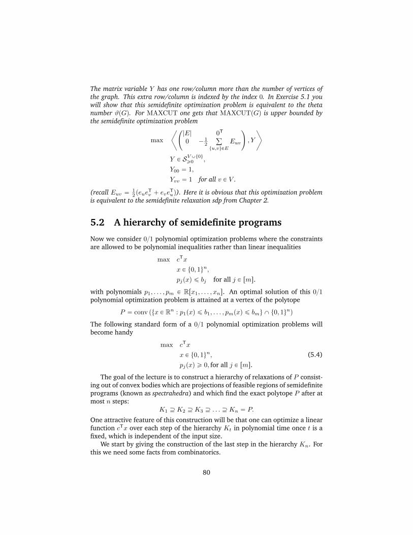
The matrix variable Y has one row/column more than the number of vertices ofthe graph. This extra row/column is indexed by the index 0. In Exercise 5.1 youwill show that this semidefinite optimization problem is equivalent to the thetanumber ϑpGq. For MAXCUT one gets that MAXCUTpGq is upper bounded bythe semidefinite optimization problem

max

C˜

|E| 0T

0 ´ 12

ř

tu,vuPE

Euv

¸

, Y

G

Y P SVYt0uě0 ,

Y00 “ 1,

Yvv “ 1 for all v P V .

(recall Euv “ 12 peue

Tv ` eve

Tuq). Here it is obvious that this optimization problem

is equivalent to the semidefinite relaxation sdp from Chapter 2.

5.2 A hierarchy of semidefinite programs

Now we consider 01 polynomial optimization problems where the constraintsare allowed to be polynomial inequalities rather than linear inequalities

max cTx

x P t0, 1un,

pjpxq ď bj for all j P rms.

with polynomials p1, . . . , pm P Rrx1, . . . , xns. An optimal solution of this 01polynomial optimization problem is attained at a vertex of the polytope

P “ conv ptx P Rn : p1pxq ď b1, . . . , pmpxq ď bmu X t0, 1unq

The following standard form of a 01 polynomial optimization problems willbecome handy

max cTx

x P t0, 1un,

pjpxq ě 0, for all j P rms.

(5.4)

The goal of the lecture is to construct a hierarchy of relaxations of P consist-ing out of convex bodies which are projections of feasible regions of semidefiniteprograms (known as spectrahedra) and which find the exact polytope P after atmost n steps:

K1 Ě K2 Ě K3 Ě . . . Ě Kn “ P.

One attractive feature of this construction will be that one can optimize a linearfunction cTx over each step of the hierarchy Kt in polynomial time once t is afixed, which is independent of the input size.

We start by giving the construction of the last step in the hierarchy Kn. Forthis we need some facts from combinatorics.

80

5.2.1 Harmonic analysis on power sets

Let X be a finite set. For many applications this will be simply X “ rns “t1, . . . , nu. By 2X we denote the set of all subsets of X, the power set of X. Thespace

L2p2Xq “ tf : 2X Ñ Ru

of real-valued functions is a Euclidean space with inner product

pf, gq “ÿ

AP2X

fpAqgpAq, with f, g P L2p2Xq.

If X “ rns then the space L2p2Xq is simply the vector space R2n and pf, gqis the standard inner product between vectors, and fpti1, . . . , ijuq is the compo-nent of the vector f with index ti1, . . . , iju.

We like to write L2p2Xq nevertheless because then resemblance with con-cepts in harmonic (Fourier) analysis, like Fourier coefficients, convolutions,functions of positive type, will become more pronounced.

Biorthogonal bases

Two explicit bases of L2p2Xq will play an important role for us.The first one is defined as follows: For B P 2X we define χB P L2p2Xq by

χBpAq “

"

1 if A Ď B,0 otherwise.

The fact that the function χB , withB P 2X , forms a basis of L2p2Xq can be easilyseen: If one considers the function χB as column vectors in R2X where we orderthe elements of 2X by increasing cardinality, then the matrix pχBqBP2X is an up-per triangular matrix in which all diagonal elements are not zero. Note that thevalue χBpAq coincides with ξpA,Bq where ξ is the zeta-function of the Booleanlattice 2X , see for instance Aigner [1, Chapter IV.1]. From the definition it isimmediate, but extremely important, that this basis is multiplicative:

χBpAYA1q “ χBpAqχBpA

1q.

The second basis is the dual basis χ˚B of χB which is defined by the biorthog-onality relation

pχB , χ˚B1q “

"

1 if B “ B1,0 otherwise.

Although we will not need it here, one can write down the second basis χ˚Bexplicitly using the Mobius function µ of the Boolean lattice 2X , namely

χ˚BpAq “ µpA,Bq “

"

p´1q|B|´|A| if A Ď B,0 otherwise.

81

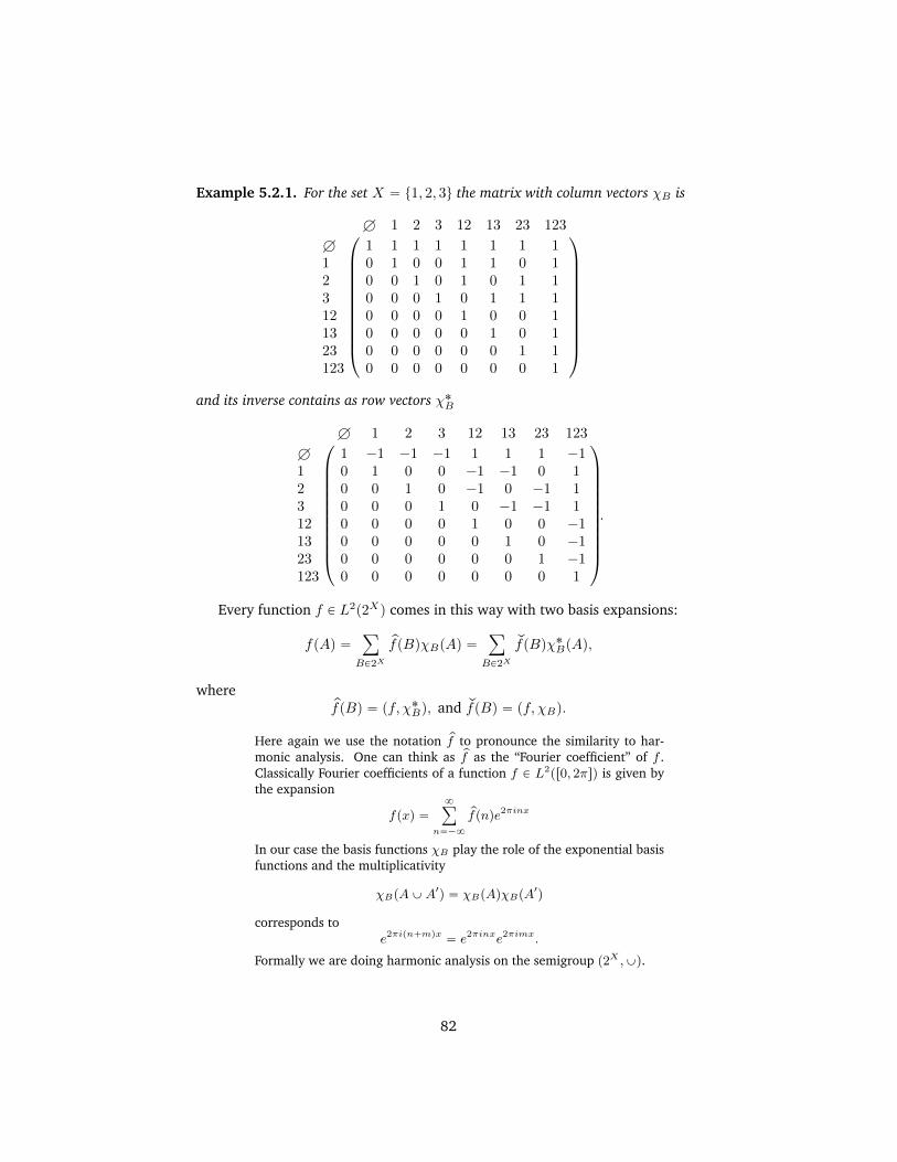
Example 5.2.1. For the set X “ t1, 2, 3u the matrix with column vectors χB is

¨

˚

˚

˚

˚

˚

˚

˚

˚

˚

˚

˝

H 1 2 3 12 13 23 123

H 1 1 1 1 1 1 1 11 0 1 0 0 1 1 0 12 0 0 1 0 1 0 1 13 0 0 0 1 0 1 1 112 0 0 0 0 1 0 0 113 0 0 0 0 0 1 0 123 0 0 0 0 0 0 1 1123 0 0 0 0 0 0 0 1

˛

‹

‹

‹

‹

‹

‹

‹

‹

‹

‹

‚

and its inverse contains as row vectors χ˚B

¨

˚

˚

˚

˚

˚

˚

˚

˚

˚

˚

˝

H 1 2 3 12 13 23 123

H 1 ´1 ´1 ´1 1 1 1 ´11 0 1 0 0 ´1 ´1 0 12 0 0 1 0 ´1 0 ´1 13 0 0 0 1 0 ´1 ´1 112 0 0 0 0 1 0 0 ´113 0 0 0 0 0 1 0 ´123 0 0 0 0 0 0 1 ´1123 0 0 0 0 0 0 0 1

˛

‹

‹

‹

‹

‹

‹

‹

‹

‹

‹

‚

.

Every function f P L2p2Xq comes in this way with two basis expansions:

fpAq “ÿ

BP2X

pfpBqχBpAq “ÿ

BP2X

qfpBqχ˚BpAq,

wherepfpBq “ pf, χ˚Bq, and qfpBq “ pf, χBq.

Here again we use the notation pf to pronounce the similarity to har-monic analysis. One can think as pf as the “Fourier coefficient” of f .Classically Fourier coefficients of a function f P L2

pr0, 2πsq is given bythe expansion

fpxq “8ÿ

n“´8

pfpnqe2πinx

In our case the basis functions χB play the role of the exponential basisfunctions and the multiplicativity

χBpAYA1q “ χBpAqχBpA

1q

corresponds toe2πipn`mqx “ e2πinxe2πimx.

Formally we are doing harmonic analysis on the semigroup p2X ,Yq.

82

We have Plancherel’s identity

pf, gq “ÿ

BP2X

pfpBqqgpBq “ÿ

BP2X

qfpBqpgpBq.

For a subset A P 2X we define the shifted function fA P L2p2Xq by

fApA1q “ fpAYA1q.

Then,pfApBq “ pfpBqχBpAq

because

fApA1q “ fpAYA1q “

ÿ

BP2X

pfpBqχBpAYA1q “

ÿ

BP2X

pfpBqχBpAqχBpA1q.

The convolution between two functions f, g P L2p2Xq is

pf ˚ gqpAq “ pf, gAq “ÿ

BP2X

qfpBqpgpBqχBpAq,

and sozf ˚ gpBq “ qfpBqpgpBq.

Note that the convolution is not commutative.

Functions of positive type

Definition 5.2.2. We say that a function f P L2p2Xq is of positive type if thesymmetric matrix Mf P S2

X

defined by

Mf pA,Bq “ fpAYBq

is positive semidefinite.

Because of the special structure of the matrix Mf , the entry Mf pA,Bq onlydepends on the union A Y B, it is sometimes called the moment matrix of f .The following theorem gives a characterization of functions of positive type.

A side remark: The theorem is in the spirit of Bochner’s theorem in har-monic analysis which says that functions of positive type are the Fouriertransform of nonnegative measures.

Theorem 5.2.3. A function f P L2p2Xq is of positive type if and only if it is of theform

fpAq “ÿ

BP2X

pfpBqχBpAq, pfpBq ě 0.

In other words, the cone of all positive semidefinite moment matrices is a polyhedralcone, even simplicial cone, with extreme rays

MBpA,A1q “ χBpAYA

1q, B P 2X .

83

Proof. One direction follows immediately from the multiplicativity of χB . Forthe other direction suppose that f P L2p2Xq has the expansion

fpAq “ÿ

BP2X

pfpBqχBpAq,

where pfpB1q ă 0 for some B1 P 2X . Then,ÿ

A,A1P2X

Mf pAYA1qχ˚B1pAqχ

˚B1pA

1q “ÿ

A,A1,BP2X

pfpBqχBpAYA1qχ˚B1pAqχ

˚B1pA

1q

“ÿ

BP2X

pfpBq

˜

ÿ

AP2X

χBpAqχ˚B1pAq

¸2

“ pfpB1q

ă 0,

hence Mf is not positive semidefinite and f is not of positive type.

5.2.2 Lasserre’s hierarchy

Now we are ready to construct the hierarchy and prove that it converges.

Equivalent reformulation

Since we are dealing with 01 problems we can assume that the polynomialsp1, . . . , pm are square free, i.e. if one considers the polynomial pi as the univari-ate polynomial in the variable xj then its degree is at most one.

We identify square free monomials

m “ xi1xi2 ¨ ¨ ¨xij P Rrx1, . . . , xns

with elements in L2p2Xq by

m “ eti1,i2,...,iju “ÿ

A:AĚti1,i2,...,iju

χ˚A P L2p2Xq,

where eti1,i2,...,iju denotes an element of the standard basis in L2pXq (so weeven work with a third basis of L2p2Xq here) and we extend this by linearity toevery square free polynomial.

Let a P t0, 1uX be a binary vector and let A P 2X be the correspondingsubset, i.e. we have ax “ 1 iff x P A. Warning: We will switch between 01vectors and subsets without (another) warning.

Then we can evaluate a square free polynomial p by

ppaq “ pp, χAq “ qppAq,

since

pm,χAq “

"

1 if ti1, . . . , iju Ď A,0 otherwise.

84

Example 5.2.4. Given are the setX “ t1, 2, 3u and the polynomial ppx1, x2, x3q “2x1 ` 3x1x2. Then

pp1, 1, 0q “ pp, χ12q “ p2pχ˚1 ` χ

˚12 ` χ

˚13 ` χ

˚123q ` 3pχ˚12 ` χ

˚123q, χ12q “ 5.

Theorem 5.2.5. Let

F “ tx P t0, 1un : p1pxq ě 0, . . . , pmpxq ě 0u

be the set of feasible solutions of the 01 polynomial optimization problem. Then afunction f P L2p2rnsq is of the form

fpAq “ÿ

bPF

pfpBqχBpAq, with pfpBq ě 0

if and only if

a) f is of positive type,

b) pj ˚ f is of positive type for all j “ 1, . . . ,m.

The geometric content of this theorem is actually pretty easy: Everyfeasible solution b P F which is a 01-vectors corresponds to a subsetB Ď t1, . . . , nu. Now we consider the cone 2rns which is spanned by allfeasible solutions, meaning it is spanned by basis vectors χB where Bcorresponds to b P F . This is a polyhedral cone with |F | extreme raysRě0χB . Now the Theorem says that f P L2

p2rnsq is an element of thispolyhedral cone iff conditions a) and b) are fulfilled. The advantageof these two conditions is that they have an equivalent formulation interms of semidefinite matrices, namely that the moment matrices Mf

and Mpj˚f are positive semidefinite.

Proof. We haveppj ˚ fqpAq “

ÿ

BP2X

qpjpBq pfpBqχBpAq.

Suppose conditions a) and b) are satisfied. By Theorem 5.2.3 the function f canbe represented as

fpAq “ÿ

BP2X

pfpBqχBpAq

with pfpBq ě 0. If strict inequality pfpBq ą 0 holds for some B then for everyj P t1, . . . ,mu we have again by Theorem 5.2.3

qpjpBq pfpBq “ pjpbq pfpBq ě 0,

because pj ˚ f is of positive type. Thus, pjpbq ě 0 for all j and hence b P F . Theother implication follows with the same arguments.

85

Corollary 5.2.6. The 01 polynomial optimization problem (5.4) is equivalent tothe linear optimization problem

maxnÿ

i“1

cifptiuq

f P L2p2Xq is of positive type,fpHq “ 1,

pj ˚ f is of positive type for all j P rms,

which is equivalent to the semidefinite program

maxnÿ

i“1

ciMf ptiu, tiuq

Mf P S2X

ě0 ,

Mf pH,Hq “ 1,

Mpj˚f P S2X

ě0 for all j P rms.

Proof. The fact that these two optimization problems are equivalent followsimmediately from the definition of positive type functions.

Since we are maximizing a linear function we can assume that the optimumf0 of the first problem is attained at the extreme ray of the cone of positive typefunctions. So it is of the form

f0 “ αχB

for some α ě 0 and by the previous theorem for some b with pjpbq ě 0 for allj P rms. Furthermore,

1 “ f0pHq “ αχBpHq “ α

makes sure that one can recover an optimal 01 solution from f0. The objectivevalue is

nÿ

i“1

cifptiuq “nÿ

i“1

ciχBptiuq.

Probabilistic interpretation

The two conditions fpHq “ 1 and f is of positive type have a simple probabilis-tic interpretation: The second condition says that f is the Fourier transform ofa positive measure whereas the first condition says that the positive measure isin fact a probability measure

1 “ fpHq “ÿ

BP2X

pfpBqχBpHq “ÿ

BP2X

pfpBq.

Hence, f determines a probability distribution on the power set 2X . The set Bis picked with probability pfpBq.

86

Relaxation

Computationally, the equivalent reformulation in Corollary 5.2.6 is a rather use-less statement: We exponentially increased the dimension of the problem andso in a sense we are enumerating all feasible solutions. However, the reformu-lation can be used to generate systematically valid non-linear inequalities, i.e.projected LMI inequalities, for the 01 polytope P “ convF .

Instead of working with full moment matrices lying in S2Xě0 we only considerin the t-th step/round of Lasserre’s hierarchy truncated moment matrices wherethe rows/columns are indexed by all subsets with cardinality at most t ` 1;Notation:

`

Xďt`1

˘

.

For f P RpX

ď2t`2q define the truncated moment matrix M t`1f P Sp

Xďt`1q by

M t`1f pA,Bq “ fpAYBq

with A,B P`

Xďt`1

˘

. Let p be a squarefree polynomial of degree d

p “ÿ

I

pImI

with coefficients pI and monomials mI where I runs through a subset J of 2X

where every I P J has cardinality at most d. Then,

Mt`1´rd2s

p˚f pA,Bq “ pp ˚ fqpAYBq “ÿ

I

pIfpI YAYBq

with A,B P`

Xďt`1´rd2s

˘

.

Definition 5.2.7. Let p1, . . . , pm P Rrx1, . . . , xns be polynomials with degreesd1, . . . , dm. Furthermore, let

v “ max trdj2s : j P rmsu .

We define for t ě v ´ 1 the t-th step in Lasserre’s hierarchy by

Kt “ tpfpt1uq, . . . , fptnuqqT P Rn : f P Rp

Xď2t`2q,

fpHq “ 1,

M t`1f ľ 0,

Mt`1´rdj2s

pj˚fľ 0, j P rms

)

.

Optimizing over Kt can be done in polynomial time once t ě v´ 1 is a fixedconstant, i.e. independent of the input size. By the previous considerations wehave

Kv´1 Ě Kv Ě Kv`1 Ě . . . Ě Kn`v´1 “ P.

87

5.2.3 Example: Independence number

Let us apply Lasserre’s hierarchy to the problem of finding the independencenumber.

For this we consider the polynomials

puvpxq “ 1´ xu ´ xv P Rrxv : v P V s for all tu, vu P E.

The 01 polytope

P “ STpGq “ convtx P t0, 1uV : puv ě 0 for all tu, vu P Eu

is called the stable set polytope1.The following theorem says that one can simplify the conditions of Kt here.

In fact the semidefinite conditions on the matrices M tpuv˚f

can be replaced bythe conditions fptu, vuq “ 0 in the moment matrix M t`1

f .

Theorem 5.2.8. For t ě 1 and f P`

Vď2t`2

˘

the following three statements areequivalent:

a) M t`1f ľ 0 and M t`1

puv˚fľ 0 for all tu, vu P E,

b) M t`1f ľ 0 and fptu, vuq “ 0 for every tu, vu P E,

c) M t`1f ľ 0 and fpUq “ 0 for every subset U P

`

Vď2t`2

˘

of the vertex set whichis not an independent set.

Proof. From M t`1f ľ 0 we can conclude that fpUq ě 0 for all U P

`

Vď2t`2

˘

because fpUq is a diagonal element of the positive semidefinite matrix M t`1f .

a) implies b): Consider the ptuu, tuuq-entry of M tpuv˚f

. It equals (check thisidentity!)

puv ˚ fptuuq “ ´fptu, vuq

Since it is a diagonal entry, it has to be non-negative. So fptu, vuq “ 0.

b) implies c): Suppose u, v P U are connected by an edge.First case: |U | ď t ` 1, then the ptu, vu, tu, vuq-entry of M t`1

f equals 0, andso the ptu, vu, Uq-entry, too (why?). Hence also fpUq “M t`1

f pU,Uq “ 0.Second case: |U | ą t` 1. Split U into U “ U1YU2 with U1, U2 P

`

Vďt`1

˘

andassume tu, vu Ď U1. Then,

M t`1f pU1, U1q “ 0 ùñM t`1

f pU1, U2q “ 0 ùñ fpUq “M t`1f pU,Uq “ 0.

c) implies a): We shall prove that the matrix M tpuv˚f

is positive semidefinite.Define P0 “

`

V ztu,vuďt

˘

and Pw “ tU Y twu : U P P0u for w P tu, vu. Then, the

1Sometimes independent sets are called stable sets, but who prefers stability over independence?

88

principal submatrix of M t`1f indexed by P0 Y Pu Y Pv is of the form

¨

˝

P0 Pu Pu

P0 C A BPu A A 0Pv B 0 B

˛

‚.

Since this matrix is positive semidefinite by assumption it follows that the matrixC Á´B is positive semidefinite because

¨

˝

´xxx

˛

‚

T¨

˝

C A BA A 0B 0 B

˛

‚

¨

˝

´xxx

˛

‚“ xTpC Á´Bqx.

Now consider the matrix M tpuv˚f

where we partition the rows/columns into P0

and its complement P 10 “`

Vďt`1

˘

zP0. It has the form

ˆ

P0 P 10P0 C Á´B 0P 10 0 0

˙

and the result follows.

One can show (Exercise 5.1.c)) that Lasserre’s hierarchy already convergesat step αpGq ´ 1 to STpGq:

Theorem 5.2.9. For a graph G with αpGq ě 2 we have

STpGq “ KαpGq´1.

5.3 Further reading

Shor [4] was the first who realized that one can use semidefinite programmingto relax quadratic optimization problems. Meanwhile there are many differentpossibilities available to construct semidefinite programming hierarchies for 01polynomial optimization problems. The one we studied in Section 5.2 is dueto Lasserre [2]. Lasserre’s hierarchy and other hierarchies are presented andcompared by Laurent in [3].

89

5.4 Exercises

5.1.** a) Show that the following two semidefinite programs give the sameoptimal value:

maxÿ

vPV

Yvv

Y P SVYt0uě0 ,

Y00 “ 1,

Y0v “ Yvv for all v P V ,

Yuv “ 0 for all tu, vu P E,

and

ϑpGq “ max xJ,Xy

X P SVě0,

xI,Xy “ 1,

Xuv “ 0 for all tu, vu P E.

b) Prove that the theta number of the cycle graph with five vertices C5

is exactly?

5.

c) Show that KαpGq´1 “ STpGq.

d) True or false? For all graphs G “ pV,Eq the following equality holds

ϑpGq “ max

#

ÿ

vPV

xv : x P K1

+

.

5.2. (Computer exercise)

a) Do the following two ellipsoids intersect?

E1 “

$

&

%

x P R3 : xT

¨

˝

19 19 1919 1336 133619 1336 4936

˛

‚x ď 1

,

.

-

,

E2 “

$

’

&

’

%

x P R3 : xT

¨

˝

?2

?2

?2

?2 2

?2 2

?2

?2 2

?2 2

?2` 1

˛

‚x`

¨

˝

´6?

2

´10?

2

´10?

2

˛

‚

T

x ď 1´ 13?

2

,

/

.

/

-

Solve a semidefinite program to justify your answer.

b) Let x1, . . . , xN be N points in R2. Find a point x P R2 which min-imizes the maximum Euclidean distance to these points. Computethe point x for the cities Amsterdam, Athens, Berlin, Copenhagen,Lisbon, Moscow, Prague, Warsaw. For this assume that Europe is partof flatland. . .

90

BIBLIOGRAPHY

[1] M. Aigner, Combinatorial theory, Springer, 1979.

[2] J.B. Lasserre, An explicit exact SDP relaxation for nonlinear 0-1 programs,pp. 293–303 in Integer Programming and Combinatorial Optimization,8th International IPCO Conference (K. Aardal, A.M.H. Gerards, ed.).,Springer, 2001.

[3] M. Laurent, A comparison of the Sherali-Adams, Lovasz-Schrijver andLasserre relaxations for 0-1 programming, Math. Oper. Res. 28 (2003),470–496.

http://www.cwi.nl/~monique/files/lasserrefinal.ps

[4] N.Z. Shor, Quadratic optimization problems, Soviet J. Comput. SystemsSci. 25 (1987), 1–11.

91

http://www.cwi.nl/~monique/files/lasserrefinal.ps

CHAPTER 6

GRAPH COLORING ANDINDEPENDENT SETS

In this chapter we revisit in detail the theta number ϑpGq, which has alreadybeen introduced in earlier chapters. In particular, we present several equivalentformulations for ϑpGq, we discuss its geometric properties, and present someapplications: for bounding the Shannon capacity of a graph, and for comput-ing in polynomial time maximum stable sets and minimum colorings in perfectgraphs.

Here are some additional definitions used in this chapter. Let G “ pV,Eq bea graph. Then, E denotes the set of pairs ti, ju of distinct nodes that are notadjacent in G. The graph G “ pV,Eq is called the complementary graph of G. Gis self-complementary if G and G are isomorphic graphs. Given a subset S Ď V ,GrSs denotes the subgraph induced by S: its node set is S and its edges are allpairs ti, ju P E with i, j P S. The graph Cn is the circuit (or cycle) of length n,with node set rns and edges the pairs ti, i`1u (for i P rns, indices taken modulon). For a set S Ď V , its characteristic vector is the vector χS P t0, 1uV , whosei-th entry is 1 if i P S and 0 otherwise. As before, e denotes the all-ones vector.

6.1 Preliminaries on graphs

6.1.1 Stability and chromatic numbers

A subset S Ď V of nodes is said to be stable (or independent) if no two nodesof S are adjacent in G. Then the stability number of G is the parameter αpGqdefined as the maximum cardinality of an independent set in G.

92

A subset C Ď V of nodes is called a clique if every two distinct nodes in Care adjacent. The maximum cardinality of a clique in G is denoted ωpGq, theclique number of G. Clearly,

ωpGq “ αpGq.

Computing the stability number of a graph is a hard problem: Given a graphG and an integer k, deciding whether αpGq ě k is an NP -complete problem.

Given an integer k ě 1, a k-coloring of G is an assignment of numbers (viewthem as colors) from t1, ¨ ¨ ¨ , ku to the nodes in such a way that two adjacentnodes receive distinct colors. In other words, this corresponds to a partition ofV into k stable sets: V “ S1 Y ¨ ¨ ¨ Y Sk, where Si is the stable set consisting ofall nodes that received the i-th color. The coloring (or chromatic) number is thesmallest integer k for which G admits a k-coloring, it is denoted as χpGq.

Again it is anNP -complete problem to decide whether a graph is k-colorable.In fact, it is NP -complete to decide whether a planar graph is 3-colorable. Onthe other hand, it is known that every planar graph is 4-colorable – this is thecelebrated 4-color theorem. Moreover, observe that one can decide in polyno-mial time whether a graph is 2-colorable, since one can check in polynomialtime whether a graph is bipartite.

Figure 6.1: The Petersen graph has αpGq “ 4, ωpGq “ 2 and χpGq “ 3

Clearly, any two nodes in a clique of G must receive distinct colors. There-fore, for any graph, the following inequality holds:

ωpGq ď χpGq. (6.1)

This inequality is strict, for example, when G is an odd circuit, i.e., a circuitof odd length at least 5, or its complement. Indeed, for an odd circuit C2n`1

(n ě 2), ωpC2n`1q “ 2 while χpC2n`1q “ 3. Moreover, for the complementG “ C2n`1, ωpGq “ n while χpGq “ n ` 1. For an illustration see the cycle oflength 7 and its complement in Figure 6.2.

6.1.2 Perfect graphs

It is intriguing to understand for which graphs equality ωpGq “ χpGq holds.Note that any graph G with ωpGq ă χpGq can be embedded in a larger graph G

93

Figure 6.2: For C7 and its complement C7: ωpC7q “ 2, χpC7q “ 3, ωpC7q “

αpC7q “ 3, χpC7q “ 4

with ωpGq “ χpGq, simply by adding toG a clique of size χpGq. This justifies thefollowing definition, introduced by C. Berge in the early sixties, which makesthe problem well posed.

Definition 6.1.1. A graph G is said to be perfect if equality

ωpHq “ χpHq

holds for all induced subgraphs H of G (including H “ G).

For instance, bipartite graphs are perfect. It follows from the definition andthe above observation about odd circuits that if G is a perfect graph then it doesnot contain an odd circuit of length at least 5 or its complement as an inducedsubgraph. Berge already conjectured that all perfect graphs arise in this way.Resolving this conjecture has haunted generations of graph theorists. It wasfinally settled in 2004 by Chudnovsky, Robertson, Seymour and Thomas whoproved the following result, known as the strong perfect graph theorem:

Theorem 6.1.2. (The strong perfect graph theorem) A graph G is perfect ifand only if it does not contain an odd circuit of length at least 5 or its complementas an induced subgraph.

This implies the following structural result about perfect graphs, known asthe perfect graph theorem, already proved by Lovasz in 1972.

Theorem 6.1.3. (The perfect graph theorem) If G is a perfect graph, then itscomplement G too is a perfect graph.

We will mention below some other, more geometric, characterizations ofperfect graphs.

6.2 Linear programming bounds

Let STpGq denote the polytope in RV defined as the convex hull of the charac-teristic vectors of the stable sets of G:

STpGq “ convtχS : S Ď V, S is a stable set in Gu,

94

called the stable set polytope of G. Hence, computing αpGq is linear optimizationover the stable set polytope:

αpGq “ maxteTx : x P STpGqu.

We have now defined the stable set polytope by listing explicitly its extremepoints. Alternatively, it can also be represented by its hyperplanes representa-tion, i.e., in the form

STpGq “ tx P RV : Ax ď bu

for some matrix A and some vector b. As computing the stability number isa hard problem one cannot hope to find the full linear inequality descriptionof the stable set polytope (i.e., the explicit A and b). However some partialinformation is known: several classes of valid inequalities for the stable setpolytope are known. For instance, if C is a clique of G, then the clique inequality

xpCq “ÿ

iPC

xi ď 1 (6.2)

is valid for STpGq: any stable set can contain at most one vertex from the cliqueC. The clique inequalities define the polytope

QSTpGq “

x P RV : x ě 0, xpCq ď 1 @C clique of G(

(6.3)

and maximizing the linear function eTx over it gives the parameter

α˚pGq “ maxteTx : x P QSTpGqu, (6.4)

known as the fractional stability number of G. Clearly, QSTpGq is a relaxation ofthe stable set polytope:

STpGq Ď QSTpGq. (6.5)

The parameter α˚pGq is nested between αpGq and χpGq, and it can also beinterpreted in terms of fractional colorings of G.

Lemma 6.2.1. For any graph G, we have

αpGq ď α˚pGq ď χpGq, (6.6)

and α˚pGq is equal to the optimal value of the linear program

min

$

&

%

ÿ

C clique of G

yC :ÿ

C clique of G

yCχC “ e, yC ě 0 @C clique of G

,

.

-

. (6.7)

Proof. The left most inequality in (6.6) follows from the inclusion (6.5) and theright most one from the definitions: If x P QSTpGq and V “ C1 Y ¨ ¨ ¨ Y Ck is apartition into k cliques, then

xTe “ xT

˜

kÿ

i“1

χCi

¸

“

kÿ

i“1

xpCiq ďkÿ

i“1

1 “ k.

95

We now show that the optimal value of (6.7) is equal to α˚pGq. For this, firstnote that in the linear program (6.4) the condition x ě 0 can be removedwithout changing the optimal value; that is,

α˚pGq “ maxteTx : xpCq ď 1 @C clique of Gu.

Now, applying linear programming duality to this linear program, we obtain thelinear program (6.7).

For instance, for an odd circuit C2n`1 (n ě 2), α˚pC2n`1q “2n`1

2 (check it)lies strictly between αpC2n`1q “ n and χpC2n`1q “ n` 1.

Assume that G is a perfect graph. Then equality holds throughout in relation(6.6). Hence, when w P RV is the all-ones vector, maximizing the objectivefunction wTx over the stable set polytope STpGq or over its linear relaxationQSTpGq gives the same optimal values. The same holds if w is 01 valued sincethis amounts to replacing G by its subgraph induced by the set of nodes withwv “ 1, which is again perfect. One can show that the same holds for anyinteger vector w P ZVě0, which implies that the two polytopes STpGq and QSTpGqcoincide. Moreover, this property characterizes perfect graphs.

Theorem 6.2.2. A graph G is perfect if and only if STpGq “ QSTpGq.

Although an explicit linear inequality description is known for the stableset polytope of a perfect graph (given by the clique inequalities), it is not clearhow to use this information in order to give an efficient algorithm for optimizingover the stable set polytope. As we see later in Section 6.5.2 there is yet anotherdescription of STpGq – in terms of semidefinite programming, using the thetabody THpGq – that allows to give an efficient algorithm.

6.3 Semidefinite programming bounds

6.3.1 The theta number

Definition 6.3.1. Given a graph G “ pV,Eq, consider the following semidefiniteprogram

maxXPSn

txJ,Xy : TrpXq “ 1, Xij “ 0 @ti, ju P E, X ľ 0u . (6.8)

Its optimal value is denoted as ϑpGq, and called the theta number of G.

This parameter was introduced by Lovasz [3]. He proved the following sim-ple, but crucial result – called the Sandwich Theorem by Knuth [2] – whichshows that ϑpGq provides a bound for both the stability number of G and thechromatic number of the complementary graph G.

Theorem 6.3.2. (Lovasz’ sandwich theorem) For any graph G, we have that

αpGq ď ϑpGq ď χpGq.

96

Proof. Given a stable set S of cardinality |S| “ αpGq, define the matrix

X “1

|S|χSpχSqT P Sn.

Then X is feasible for (6.8) with objective value xJ,Xy “ |S| (check it). Thisshows the inequality αpGq ď ϑpGq.

Now, consider a matrix X feasible for the program (6.8) and a partition of Vinto k cliques: V “ C1Y¨ ¨ ¨YCk. Our goal is now to show that xJ,Xy ď k, whichwill imply ϑpGq ď χpGq. For this, using the relation e “

řki“1 χ

Ci , observe that

Y :“kÿ

i“1

`

kχCi ´ e˘ `

kχCi ´ e˘T“ k2

kÿ

i“1

χCipχCiqT ´ kJ.

Moreover,C

X,kÿ

i“1

χCipχCiqT

G

“ TrpXq.

Indeed the matrixř

i χCipχCiqT has all its diagonal entries equal to 1 and it

has zero off-diagonal entries outside the edge set of G, while X has zero off-diagonal entries on the edge set of G. As X,Y ľ 0, we obtain

0 ď xX,Y y “ k2TrpXq ´ kxJ,Xy

and thus xJ,Xy ď k TrpXq “ k.

An alternative argument for the inequality ϑpGq ď χpGq, showing an evenmore transparent link to coverings by cliques, will be given in the paragraphafter the proof of Lemma 6.4.2.

6.3.2 Computing maximum stable sets in perfect graphs

Assume that G is a graph satisfying αpGq “ χpGq. Then, as a direct applica-tion of Theorem 6.3.2, αpGq “ χpGq “ ϑpGq can be computed by solving thesemidefinite program (6.8), it suffices to solve this semidefinite program withprecision ε ă 12 as one can then find αpGq by rounding the optimal value tothe nearest integer. In particular, combining with the perfect graph theorem(Theorem 6.1.3):

Theorem 6.3.3. If G is a perfect graph then αpGq “ χpGq “ ϑpGq and ωpGq “χpGq “ ϑpGq.

Hence one can compute the stability number and the chromatic number inpolynomial time for perfect graphs. Moreover, one can also find a maximumstable set and a minimum coloring in polynomial time for perfect graphs. Wenow indicate how to construct a maximum stable set – we deal with minimumgraph colorings in the next section.

97

Let G “ pV,Eq be a perfect graph. Order the nodes of G as v1, ¨ ¨ ¨ , vn. Thenwe construct a sequence of induced subgraphsG0, G1, ¨ ¨ ¨ , Gn ofG. Hence eachGi is perfect, also after removing a node, so that we can compute in polynomialtime the stability number of such graphs. The construction goes as follows: SetG0 “ G. For each i “ 1, ¨ ¨ ¨ , n do the following:

1. Compute αpGi´1zviq.

2. If αpGi´1zviq “ αpGq, then set Gi “ Gi´1zvi.

3. Otherwise, set Gi “ Gi´1.

By construction, αpGiq “ αpGq for all i. In particular, αpGnq “ αpGq. Moreover,the node set of the final graph Gn is a stable set and, therefore, it is a maximumstable set of G. Indeed, if the node set of Gn is not stable then it contains a nodevi for which αpGnzviq “ αpGnq. But then, asGn is an induced subgraph ofGi´1,one would have that αpGnzviq ď αpGi´1zviq and thus αpGi´1zviq “ αpGq, sothat node vi would have been removed at Step 2.

Hence, the above algorithm permits to construct a maximum stable set ina perfect graph G in polynomial time – namely by solving n ` 1 semidefiniteprograms for computing αpGq and αpGi´1zviq for i “ 1, ¨ ¨ ¨ , n.

More generally, given integer weights w P ZVě0 on the nodes, one can com-pute in polynomial time a stable set S of maximum weight wpSq. For this, onecan apply the algorithm just described for computing a maximum cardinalitystable set in the new graph G1 defined in the following way: Replace each nodei P V by a set Wi of wi nodes pairwise non-adjacent, and make two nodesx P Wi and y P Wj adjacent if i and j are adjacent in G. One can verify that G1

is perfect and that αpG1q is the maximum weight wpSq of a stable set S in G.

6.3.3 Minimum colorings of perfect graphs

We now describe an algorithm for computing a minimum coloring of a perfectgraph G in polynomial time. This will be reduced to several computations ofthe theta number which we will use for computing the clique number of someinduced subgraphs of G.

Let G “ pV,Eq be a perfect graph. Call a clique of G maximum if it hasmaximum cardinality ωpGq.

The crucial observation is that it suffices to find a stable set S in G whichmeets all maximum cliques. Indeed, if such S is found then one can recursivelycolor GzS with ωpGq ´ 1 colors (in polynomial time), and thus G with ωpGqcolors. (Clearly, such a stable set S exists: any color class S in a ωpGq-coloringmust meet all maximum cliques as ωpGzSq “ χpGzSq “ ωpGq ´ 1.)

The algorithm goes as follows: For t ě 1, grow a list L of t maximum cliquesC1, ¨ ¨ ¨ , Ct. Suppose C1, ¨ ¨ ¨ , Ct have been found. Then do the following:

1. We find a stable set S meeting each of the cliques C1, ¨ ¨ ¨ , Ct (see below).

98

2. Compute ωpGzSq.

3. If ωpGzSq ă ωpGq then S meets all maximum cliques and we are done.

4. Otherwise, compute a maximum clique Ct`1 in GzS, which is thus a newmaximum clique of G, and we add it to the list L.

The first step can be done as follows: Set w “řti“1 χ

Ci P ZVě0 and computea stable set S having maximum possible weight wpSq, then wpSq “ t and Smeets C1, ¨ ¨ ¨ , Ct.

The above algorithm has polynomial running time, since the number of iter-ations is bounded by |V |. To see this, define the affine space Lt Ď RV definedby the equations xpC1q “ 1, ¨ ¨ ¨ , xpCtq “ 1 corresponding to the cliques in thecurrent list L. Then, Lt contains strictly Lt`1, since χS P LtzLt`1 for the set Sconstructed in the first step, and thus the dimension decreases at least by 1 ateach iteration.

6.4 Other formulations of the theta number

6.4.1 Dual formulation

We now give several equivalent formulations for the theta number obtained byapplying semidefinite programming duality and some further elementary ma-nipulations.

Lemma 6.4.1. The theta number can be expressed by any of the following pro-grams:

ϑpGq “ mintPR,APSn

tt : tI À´ J ľ 0, Aij “ 0 pi “ j or ti, ju P Equ, (6.9)

ϑpGq “ mintPR,BPSn

t : tI ´B ľ 0, Bij “ 1 pi “ j or ti, ju P Eq(

, (6.10)

ϑpGq “ mintPR,CPSn

tt : C ´ J ľ 0, Cii “ t pi P V q, Cij “ 0 pti, ju P Equ, (6.11)

ϑpGq “ minBPSn

λmaxpBq : Bij “ 1 pi “ j or ti, ju P Eq(

. (6.12)

Proof. First we build the dual of the semidefinite program (6.8), which reads:

mintPR,yPRE

$

&

%

t : tI `ÿ

ti,juPE

yijEij ´ J ľ 0

,

.

-

. (6.13)

As both programs (6.8) and (6.13) are strictly feasible, there is no duality gap:the optimal value of (6.13) is equal to ϑpGq, and the optimal values are attainedin both programs – here we have applied the duality theorem (Theorem 3.4.1).

Setting A “ř

ti,juPE yijEij , B “ J Á and C “ tI À in (6.13), it followsthat the program (6.13) is equivalent to (6.9), (6.10) and (6.11). Finally theformulation (6.12) follows directly from (6.10) after recalling that λmaxpBq isthe smallest scalar t for which tI ´B ľ 0.

99

6.4.2 Two more (lifted) formulations

We give here two more formulations for the theta number. They rely on semidef-inite programs involving symmetric matrices of order 1`n which we will indexby the set t0u Y V , where 0 is an additional index that does not belong to V .

Lemma 6.4.2. The theta number ϑpGq is equal to the optimal value of the follow-ing semidefinite program:

minZPSn`1

tZ00 : Z ľ 0, Z0i “ Zii “ 1 pi P V q, Zij “ 0 pti, ju P Equ. (6.14)

Proof. We show that the two semidefinite programs in (6.9) and (6.14) areequivalent. For this, observe that

tI `A´ J ľ 0 ðñ Z :“

ˆ

t eT

e I ` 1tA

˙

ľ 0,

which follows by taking the Schur complement of the upper left corner t in theblock matrix Z. Hence, if pt, Aq is feasible for (6.9), then Z is feasible for (6.14)with same objective value: Z00 “ t. The construction can be reversed: if Z isfeasible for (6.14), then one can construct pt, Aq feasible for (6.9) with t “ Z00.Hence both programs are equivalent.

From the formulation (6.14), the link to the chromatic number is even moretransparent. Indeed, let k “ χpGq and consider a partition V “ C1Y ¨ ¨ ¨YCk ofthe node set into k cliques. For each clique Ci define the extended characteristicvector zi “ p1 χCiq P R1`n obtained by appending an entry 1 to the character-istic vector of Ci. Define the matrix Z “

řki“1 ziz

Ti P S1`n. Then one can easily

check that the matrix Z is feasible for the program (6.14) with objective valueZ00 “ k. Hence this shows again the inequality ϑpGq ď χpGq.

Applying duality to the semidefinite program (6.14), we obtain1 the follow-ing formulation for ϑpGq.

Lemma 6.4.3. The theta number ϑpGq is equal to the optimal value of the follow-ing semidefinite program:

maxY PSn`1

#

ÿ

iPV

Yii : Y ľ 0, Y00 “ 1, Y0i “ Yii pi P V q, Yij “ 0 pti, ju P Eq

+

.

(6.15)

Proof. One can verify that the dual program of (6.14) reads

max

#

´ÿ

iPV

Yii ` 2Y0i : Y ľ 0, Y00 “ 1, Yij “ 0 pti, ju P Eq

+

(6.16)

1Of course there is more than one road leading to Rome: one can also show directly the equiva-lence of the two programs (6.8) and (6.15).

100

(check it). As (6.14) is strictly feasible (check it) there is no duality gap, theoptimal value of (6.16) is attained and it is equal to ϑpGq. Note that the pro-gram (6.15) amounts to adding the constraints Yii “ Y0i (i P V ) to the program(6.16). In order to show that both programs (6.15) and (6.16) are equivalent,it suffices to show that (6.16) admits an optimal solution satisfying these addi-tional constraints.

For this pick an optimal solution Y to (6.16). In a first step, we show thatY0i ` Yii “ 0 for all i P V . Indeed, assume that Y0i ` Yii ‰ 0 for some i P V .Then, Yii ‰ 0. Let us multiply the i-th column and the i-th row of the matrix Yby the scalar ´X0i

Xii. In this way we obtain a new matrix Y 1 which is still feasible

for (6.16), but with a better objective value: Indeed, Y 1ii “ Yii

´

Ý0i

Yii

¯2

“Y 20i

Yii

and Y 10i “ Ý 20i

Yii, so that the i-th term in the new objective value is

´pY 1ii ` 2Y 10iq “Y 20i

Yiią ´pYii ` 2Y0iq.

Hence, Y0i “ Ýii for all i P V . Now, we can change the signs on the first rowand column of Y (indexed by the index 0). In this way we obtain a new optimalsolution of (6.16) which now satisfies the conditions: Yii “ Y0i for i P V .

As explained in Chapter 5 one can define a hierarchy of semidefinite boundsfor αpGq, strengthening the theta number ϑpGq. While ϑpGq is defined usingmatrices indexed by t0uYV , these stronger bounds are obtained by consideringmatrices indexed by larger index sets, thus lifting the problem in even largerdimensions – see Section 5.2.3 for details.

6.5 Geometric properties of the theta number

6.5.1 Orthonormal representations

Definition 6.5.1. An orthonormal representation ofG, abbreviated as ONR, con-sists of a set of unit vectors tu1, . . . , unu Ď Rd (for some d ě 1) satisfying

uTi uj “ 0 @ti, ju P E.

If S is a stable set in G and the ui’s form an ONR of G of dimension d, thenthe vectors ui labeling the nodes of S are pairwise orthogonal, which impliesthat d ě αpGq. It turns out that the stronger lower bound: d ě ϑpGq holds.

Lemma 6.5.2. The minimum dimension d of an orthonormal representation of agraph G satisfies: ϑpGq ď d.

Proof. Let u1, ¨ ¨ ¨ , un P Rd be an ONR of G. Define the matrices U0 “ Id,Ui “ uiu

Ti P Sd for i P rns. Now we define a symmetric matrix Z P Sn`1 by

setting Zij “ xUi, Ujy for i, j P t0uYrns. One can verify that Z is feasible for theprogram (6.14) defining ϑpGq (check it) with Z00 “ d. This gives ϑpGq ď d.

101

6.5.2 The theta body THpGq

It is convenient to introduce the following set of matrices X P Sn`1, wherecolumns and rows are indexed by the set t0u Y V :

MG “ tY P Sn`1 : Y00 “ 1, Y0i “ Yii pi P V q, Yij “ 0 pti, ju P Eq, Y ľ 0u,(6.17)

which is thus the feasible region of the semidefinite program (6.15). Now letTHpGq denote the convex set obtained by projecting the setMG onto the sub-space RV of the diagonal entries:

THpGq “ tx P RV : DY PMG such that xi “ Yii @i P V u, (6.18)

called the theta body of G. It turns out that THpGq is nested between STpGq andQSTpGq.

Lemma 6.5.3. For any graph G, we have that STpGq Ď THpGq Ď QSTpGq.

Proof. The inclusion STpGq Ď THpGq follows from the fact that the characteris-tic vector of any stable set lies in THpGq (check it). We now show the inclusionTHpGq Ď QSTpGq. For this pick a vector x P THpGq and a clique C of G; weshow that xpCq ď 1. Say xi “ Yii for all i P V , where Y PMG. Consider theprincipal submatrix YC of Y indexed by t0u Y C, which is of the form

YC “

ˆ

1 xTCxC DiagpxCq

˙

,

where we set xC “ pxiqiPC . Now, YC ľ 0 implies that DiagpxCq ´ xCxTC ľ 0

(taking a Schur complement). This in turn implies: eTpDiagpxCq´xCxTCqe ě 0,which can be rewritten as xpCq ´ pxpCqq2 ě 0, giving xpCq ď 1.

In view of Lemma 6.4.3, maximizing the all-ones objective function overTHpGq gives the theta number:

ϑpGq “ maxxPRV

teTx : x P THpGqu.

As maximizing eTx over QSTpGq gives the LP bound α˚pGq, Lemma 6.5.3 im-plies directly that the SDP bound ϑpGq dominates the LP bound α˚pGq:

Corollary 6.5.4. For any graph G, we have that αpGq ď ϑpGq ď α˚pGq.

Combining the inclusion from Lemma 6.5.3 with Theorem 6.2.2, we deducethat THpGq “ STpGq “ QSTpGq for perfect graphs. It turns out that theseequalities characterize perfect graphs.

Theorem 6.5.5. For any graph G the following assertions are equivalent.

1. G is perfect.

2. THpGq “ STpGq

3. THpGq “ QSTpGq.

4. THpGq is a polytope.

102

6.5.3 More on the theta body

There is a beautiful relationship between the theta bodies of a graph G and ofits complementary graph G:

Theorem 6.5.6. For any graph G,

THpGq “ tx P RVě0 : xT z ď 1 @z P THpGqu.

In other words, we know an explicit linear inequality description of THpGq;moreover, the normal vectors to the supporting hyperplanes of THpGq are pre-cisely the elements of THpGq. One inclusion is easy:

Lemma 6.5.7. If x P THpGq and z P THpGq then xTz ď 1.

Proof. Let Y PMG and Z PMG such that x “ pYiiq and z “ pZiiq. Let Z 1 beobtained from Z by changing signs in its first row and column (indexed by 0).Then xY,Z 1y ě 0 as Y,Z 1 ľ 0. Moreover, xY, Z 1y “ 1 ´ xTz (check it), thusgiving xTz ď 1.

Next we observe how the elements of THpGq can be expressed in terms oforthonormal representations of G.

Lemma 6.5.8. For x P RVě0, x P THpGq if and only if there exist an orthonormalrepresentation v1, . . . , vn of G and a unit vector d such that x “ ppdTviq2qiPV .

Proof. Let d, vi be unit vectors where the vi’s form an ONR of G; we show thatx “ ppdTviq

2q P THpGq. For this, let Y P Sn`1 denote the the Gram matrix of thevectors d and pvTi dqvi for i P V , so that x “ pYiiq. One can verify that Y PMG,which implies x P THpGq.

For the reverse inclusion, pick Y P MG and a Gram representation w0, wi(i P V ) of Y . Set d “ w0 and vi “ wiwi for i P V . Then the conditionsexpressing membership of Y in MG imply that the vi’s form an ONR of G,d “ 1, and Yii “ pdTviq2 for all i P V .

To conclude the proof of Theorem 6.5.6 we use the following result, whichcharacterizes which partially specified matrices can be completed to a positivesemidefinite matrix – you will prove it in Exercise 6.1.

Proposition 6.5.9. Let H “ pW,F q be a graph and let aij (i “ j P W orti, ju P F ) be given scalars, corresponding to a vector a P RWYF . Define theconvex set

Ka “ tY P SW : Y ľ 0, Yij “ aij @i “ j PW and ti, ju P F u (6.19)

(consisting of all possible positive semidefinite completions of a) and the cone

CH “ tZ P SW : Z ľ 0, Zij “ 0 @ti, ju P F u (6.20)

(consisting of all positive semidefinite matrices supported by the graph H). Then,Ka ‰ H if and only if

ÿ

iPW

aiiZii ` 2ÿ

ti,juPF

aijZij ě 0 @Z P CH . (6.21)

103

Proof. (of Theorem 6.5.6). Let x P RVě0 such that xTz ď 1 for all z P THpGq;we show that x P THpGq. For this we need to find a matrix Y P MG suchthat x “ pYiiqiPV . In other words, the entries of Y are specified already at thefollowing positions: Y00 “ 1, Y0i “ Yii “ xi for i P V , and Yti,ju “ 0 for allti, ju P E, and we need to show that the remaining entries (at the positions ofnon-edges of G) can be chosen in such a way that Y ľ 0.

To show this we apply Proposition 6.5.9, where the graph H is G with anadditional node 0 adjacent to all i P V . Hence it suffices now to show thatxY,Zy ě 0 for all Z P St0uYVľ0 with Zij “ 0 if ti, ju P E. Pick such Z, with Gramrepresentation w0, w1, ¨ ¨ ¨ , wn. Then wT

i wj “ 0 if ti, ju P E. We can assumewithout loss of generality that all wi are non-zero (use continuity if some wiis zero) and up to scaling that w0 is a unit vector. Then the vectors wiwi(i P V ) form an ONR of G. By Lemma 6.5.8 (applied to G), the vector z P RVwith zi “ pwT

0wiq2wi

2 belongs to THpGq and thus xTz ď 1 by assumption.Therefore, xY,Zy is equal to

1` 2ÿ

iPV

xiwT0wi `

ÿ

iPV

xiwi2 ě

ÿ

iPV

xi

ˆ

pwT0wiq

2

wi2` 2wT

0wi ` wi2

˙

“ÿ

iPV

xi

ˆ

wT0wiwi

` wi

˙2

ě 0.

6.6 The theta number for vertex-transitive graphs

First we mention an inequality relating the theta numbers of a graph and itscomplement.

Proposition 6.6.1. For any graph G “ pV,Eq, we have that ϑpGqϑpGq ě |V |.

Proof. Using the formulation of the theta number from (6.11), we obtain ma-trices C,C 1 P Sn such that C ´ J,C 1 ´ J ľ 0, Cii “ ϑpGq, C 1ii “ ϑpGq fori P V , Cij “ 0 for ti, ju P E and C 1ij “ 0 for ti, ju P E. Then, we have thatxC, Jy, xC 1, Jy ě xJ, Jy “ n2, and xC,C 1y “ nϑpGqϑpGq. Combining these factsyields the desired inequality.

We now show that equality ϑpGqϑpGq “ |V | holds for certain symmetricgraphs, namely for vertex-transitive graphs. In order to show this, one exploitsin a crucial manner the symmetry of G, which permits to show that the semidef-inite program defining the theta number has an optimal solution with a special(symmetric) structure. We need to introduce some definitions.

Let G “ pV,Eq be a graph. A permutation σ of the node set V is called anautomorphism of G if it preserves edges, i.e., ti, ju P E implies tσpiq, σpjqu P E.Then the set AutpGq of automorphisms of G is a group. The graph G is said to

104

be vertex-transitive if for any two nodes i, j P V there exists an automorphismσ P AutpGq mapping i to j: σpiq “ j.

The group of permutations of V acts on symmetric matrices X indexed byV . Namely, if σ is a permutation of V and Pσ is the corresponding permutationmatrix (with Pσpi, jq “ Pσpiq,σpjq for all i, j P V ), then one can build the newsymmetric matrix

σpXq :“ PσXPTσ “ pXσpiq,σpjqqi,jPV .

If σ is an automorphism of G, then it preserves the feasible region of thesemidefinite program (6.8) defining the theta number ϑpGq. This is an easy,but very useful fact.

Lemma 6.6.2. If X is feasible for the program (6.8) and σ is an automorphismof G, then σpXq is again feasible for (6.8), moreover with the same objective valueas X.

Proof. Directly from the fact that xJ, σpXqy “ xJ,Xy, TrpσpXqq “ TrpXq andσpXqij “ Xσpiqσpjq “ 0 if ti, ju P E (since σ is an automorphism of G).

Lemma 6.6.3. The program (6.8) has an optimal solution X˚ which is invariantunder action of the automorphism group of G, i.e., satisfies σpX˚q “ X˚ for allσ P AutpGq.

Proof. Let X be an optimal solution of (6.8). By Lemma 6.6.2, σpXq is again anoptimal solution for each σ P AutpGq. Define the matrix

X˚ “1

|AutpGq|

ÿ

σPAutpGq

σpXq,

obtained by averaging over all matrices σpXq for σ P AutpGq. As the set ofoptimal solutions of (6.8) is convex, X˚ is still an optimal solution of (6.8).Moreover, by construction, X˚ is invariant under action of AutpGq.

Corollary 6.6.4. If G is a vertex-transitive graph then the program (6.8) has anoptimal solution X˚ satisfying X˚ii “ 1n for all i P V and X˚e “ ϑpGq

n e.

Proof. By Lemma 6.6.3, there is an optimal solution X˚ which is invariantunder action of AutpGq. As G is vertex-transitive, all diagonal entries of X˚

are equal: Indeed, let i, j P V and σ P AutpGq such that σpiq “ j. Then,Xjj “ Xσpiqσpiq “ Xii. As TrpX˚q “ 1 we must have X˚ii “ 1n for all i. Analo-gously, the invariance of X˚ implies that

ř

kPV X˚ik “

ř

kPV X˚jk for all i, j, i.e.,

X˚e “ λe for some scalar λ. Combining with the condition xJ,X˚y “ ϑpGq weobtain that λ “ ϑpGq

n .

Proposition 6.6.5. If G is a vertex-transitive graph, then ϑpGqϑpGq “ |V |.

105

Proof. By Corollary 6.6.4, there is an optimal solution X˚ of the program (6.8)defining ϑpGq which satisfies X˚ii “ 1n for i P V and X˚e “ ϑpGq

n e. Thenn2

ϑpGqX˚ ´ J ľ 0 (check it). Hence, t “ n

ϑpGq and C “ n2

ϑpGqX˚ define a feasible

solution of the program (6.11) defining ϑpGq, which implies ϑpGq ď nϑpGq.Combining with Proposition 6.6.1 we get the equality ϑpGqϑpGq “ |V |.

For instance, the cycle Cn is vertex-transitive, so that

ϑpCnqϑpCnq “ n. (6.22)

In particular, as C5 is isomorphic to C5, we deduce that

ϑpC5q “?

5. (6.23)

For n even, Cn is bipartite (and thus perfect), so that ϑpCnq “ αpCnq “n2

and ϑpCnq “ ωpCnq “ 2. For n odd, one can compute ϑpCnq using the abovesymmetry reduction:

Proposition 6.6.6. For any odd n ě 3,

ϑpCnq “n cospπnq

1` cospπnqand ϑpCnq “

1` cospπnq

cospπnq.

Proof. As ϑpCnqϑpCnq “ n, it suffices to compute ϑpCnq. We use the formulation(6.12). As Cn is vertex-transitive, there is an optimal solution B whose entriesare all equal to 1, except Bij “ 1 ` x for some scalar x whenever |i ´ j| “ 1(modulo n). In other words, B “ J ` xACn , where ACn is the adjacencymatrix of the cycle Cn. Thus ϑpCnq is equal to the minimum value of λmaxpBqfor all possible x. The eigenvalues of ACn are known: They are ωk ` ω´k

(for k “ 0, 1, ¨ ¨ ¨ , n ´ 1), where ω “ e2iπn is an n-th root of unity. Hence the

eigenvalues of B are

n` 2x and xpωk ` ω´kq for k “ 1, ¨ ¨ ¨ , n´ 1. (6.24)

We minimize the maximum of the values in (6.24) when choosing x such that

n` 2x “ ´2x cospπnq

(check it). This gives ϑpCnq “ λmaxpBq “ ´2x cospπnq “ n cospπnq1`cospπnq .

6.7 Bounding the Shannon capacity

The theta number was introduced by Lovasz [3] in connection with the problemof computing the Shannon capacity of a graph, a problem in coding theoryconsidered by Shannon. We need some definitions.

106

Definition 6.7.1. (Strong product) Let G “ pV,Eq and H “ pW,F q be twographs. Their strong product is the graph denoted as G ¨H with node set V ˆWand with edges the pairs of distinct nodes tpi, rq, pj, squ P V ˆW with (i “ j orti, ju P E) and (r “ s or tr, su P F ).

If S Ď V is stable in G and T Ď W is stable in H then S ˆ T is stable inG ¨ H. Hence, αpG ¨ Hq ě αpGqαpHq. Let Gk denote the strong product of kcopies of G, we have that

αpGkq ě pαpGqqk.

Based on this, one can verify that

ΘpGq :“ supkě1

k

b

αpGkq “ limkÑ8

k

b

αpGkq. (6.25)

The parameter ΘpGq was introduced by Shannon in 1956, it is called the Shan-non capacity of the graph G. The motivation is as follows. Suppose V is a finitealphabet, where some pairs of letters could be confused when they are trans-mitted over some transmission channel. These pairs of confusable letters canbe seen as the edge set E of a graph G “ pV,Eq. Then the stability number ofG is the largest number of one-letter messages that can be sent without dan-ger of confusion. Words of length k correspond to k-tuples in V k. Two wordspi1, ¨ ¨ ¨ , ikq and pj1, ¨ ¨ ¨ , jkq can be confused if at every position h P rks the twoletters ih and jh are equal or can be confused, which corresponds to having anedge in the strong product Gk. Hence the largest number of words of length kthat can be sent without danger of confusion is equal to the stability number ofGk and the Shannon capacity of G represents the rate of correct transmission ofthe graph.

For instance, for the 5-cycle C5, αpC5q “ 2, but αppC5q2q ě 5. Indeed,

if 1, 2, 3, 4, 5 are the nodes of C5 (in this cyclic order), then the five 2-letterwords p1, 1q, p2, 3q, p3, 5q, p4, 2q, p5, 4q form a stable set in G2. This implies thatΘpC5q ě

?5.

Determining the exact Shannon capacity of a graph is a very difficult prob-lem in general, even for small graphs. For instance, the exact value of theShannon capacity of C5 was not known until Lovasz [3] showed how to use thetheta number in order to upper bound the Shannon capacity: Lovasz showedthat ΘpGq ď ϑpGq and ϑpC5q “

?5, which implies that ΘpC5q “

?5. For in-

stance, although the exact value of the theta number of C2n`1 is known (cf.Proposition 6.6.6), the exact value of the Shannon capacity of C2n`1 is notknown, already for C7.

Theorem 6.7.2. For any graph G, we have that ΘpGq ď ϑpGq.

The proof is based on the multiplicative property of the theta number fromLemma 6.7.3 – which you will prove in Exercise 6.2 – combined with the factthat the theta number upper bounds the stability number: For any integer k,αpGkq ď ϑpGkq “ pϑpGqqk implies k

a

αpGkq ď ϑpGq and thus ΘpGq ď ϑpGq.

107

Lemma 6.7.3. The theta number of the strong product of two graphs G and Hsatisfies ϑpG ¨Hq “ ϑpGqϑpHq.

As an application one can compute the Shannon capacity of any graph Gwhich is vertex-transitive and self-complementary (e.g., like C5).

Theorem 6.7.4. If G “ pV,Eq is a vertex-transitive graph, then ΘpG ¨Gq “ |V |.If, moreover, G is self-complementary, then ΘpGq “

a

|V |.

Proof. We have ΘpG ¨ Gq ě αpG ¨ Gq ě |V |, since the set of diagonal pairstpi, iq : i P V u is stable in G ¨ G. The reverse inequality follows from Lemma6.7.3 combined with Proposition 6.6.5: ΘpG ¨Gq ď ϑpG ¨Gq “ ϑpGqϑpGq “ |V |.If G is isomorphic to G then ΘpG ¨Gq “ ΘpG2q “ pΘpGqq2 (check the rightmostequality). This gives ΘpGq “

a

|V |.

6.8 Further reading

In his seminal paper [3], Lovasz gives several equivalent formulations for thetheta number, and relates it to the Shannon capacity and to some eigenvaluebounds. It is worth noting that Lovasz’ paper was published in 1979, thus be-fore the discovery of polynomial time algorithms for semidefinite programming.In 1981, together with Grotschel and Schrijver, he derived the polynomial timealgorithms for maximum stable sets and graph colorings in perfect graphs, basedon the ellipsoid method for solving semidefinite programs. As of today, this isthe only known polynomial time algorithm – in particular, no purely combina-torial algorithm is known.

Detailed information about the theta number can also be found in the surveyof Knuth [2] and a detailed treatment about the material in this chapter can befound in Chapter 9 of Grotschel, Lovasz and Schrijver [1]. In particular, proofsof the geometric characterizations of perfect graphs in Theorems 6.2.2 and 6.5.5can be found there. Weighted versions of the theta number are considered there,replacing the all-ones objective function eTx by wTx where w P ZVě0. One cangive equivalent characterizations, analogue to those we have given for the all-ones weight function. We have restricted our exposition to the all-ones weightfunction for the sake of simplicity.

6.9 Exercises

6.1 Show the result of Proposition 6.5.9.

6.2** The goal is to show the result of Lemma 6.7.3 about the theta number ofthe strong product of two graphs G “ pV,Eq and H “ pW,F q:

ϑpG ¨Hq “ ϑpGqϑpHq.

(a) Show that ϑpG ¨Hq ě ϑpGqϑpHq.

108

(b) Show that ϑpG ¨Hq ď ϑpGqϑpHq.

Hint: Use the primal formulation (6.8) for (a), and the dual formulation(6.9) for (b), and think of using Kronecker products of matrices in orderto build feasible solutions.

6.3 Let G “ pV “ rns, Eq be a graph. Consider the graph parameter

ϑ1pGq “ minc,ui

maxiPV

1

pcTuiq2,

where the minimum is taken over all unit vectors c and all orthonormalrepresentations u1, ¨ ¨ ¨ , un of G.

Show that ϑpGq “ ϑ1pGq.

Hint: For the inequality ϑpGq ď ϑ1pGq think of using the properties of thetheta body from Section 6.5.2. For the inequality ϑ1pGq ď ϑpGq, use anoptimal solution B of the dual formulation (6.10) for ϑpGq to build thevectors c, ui.

109

BIBLIOGRAPHY

[1] M. Grotschel, L. Lovasz, A. Schrijver. Geometric Algorithms in Combina-torial Optimization, Springer, 1988.

http://www.zib.de/groetschel/pubnew/paper/

groetschellovaszschrijver1988.pdf

[2] D.E. Knuth. The Sandwich Theorem. The Electronic Journal of Combina-torics 1, A1, 1994.

http://www.combinatorics.org/ojs/index.php/eljc/article/view/

v1i1a1

[3] L. Lovasz. On the Shannon capacity of a graph. IEEE Transactions onInformation Theory IT-25:1–7, 1979.

110

http://www.zib.de/groetschel/pubnew/paper/groetschellovaszschrijver1988.pdf

http://www.zib.de/groetschel/pubnew/paper/groetschellovaszschrijver1988.pdf

http://www.combinatorics.org/ojs/index.php/eljc/article/view/v1i1a1

http://www.combinatorics.org/ojs/index.php/eljc/article/view/v1i1a1

CHAPTER 7

APPROXIMATING MAX CUTAND THE CUT NORM

The maximum cut problem (MAX CUT) is the following problem in combina-torial optimization. Let G “ pV,Eq be an undirected graph with vertex set Vand edge set E Ď

`

V2

˘

, where edges e “ tu, vu P E are two-element subsets ofthe vertex set. With every edge e “ tu, vu we associate a nonnegative weightwuv. Since the graph is undirected we assume that the weights are symmetricwuv “ wvu. Furthermore, wuv “ 0 whenever tu, vu R E. We incorporate allthe weights into a symmetric matrix W “ pwuvq P SV . The MAX CUT problemseeks for a partition of the vertex set V into two parts V ´, V `, cutting the graphinto two pieces, so that the sum of edges connecting V ´ and V `, the weight ofthe cut wpV ´, V `q, is maximized:

wpV ´, V `q “ÿ

uPV ´,vPV `

wuv.

It is known that the maximum cut problem is an NP-complete problem. Sounless the complexity classes P and NP coincide there is no efficient polynomial-time algorithm which solves MAX CUT exactly. In fact, MAX CUT was one ofthe first problems which were proved to be NP-complete: It is one of Karp’s 21NP-complete problems. Even stronger, Hastad in 2001 showed that it is NP-hardto approximate MAX CUT within a factor of 16

17 “ 0.941 . . . This is in sharpcontrast to the MIN CUT problem, where we want to minimize the weight of anon-trivial cut. The MIN CUT problem (and its dual, the MAX FLOW problem)can be solved using linear programming.

On the positive side, one can compute an 0.878 . . . -approximation of MAXCUT in polynomial time, using semidefinite programming. This algorithm, due

111

to Goemans and Williamson [2], is one of the most influential approximationalgorithms which are based on semidefinite programming.

A problem which is related to (in fact a generalization of) MAX CUT is find-ing the cut norm of a matrix. Let A “ pAijq P Rmˆn be a real matrix. The cutnorm of A is

Al “ maxIĎrms,JĎrns

ˇ

ˇ

ˇ

ˇ

ˇ

ÿ

iPI

ÿ

jPJ

Aij

ˇ

ˇ

ˇ

ˇ

ˇ

.

Computing the cut norm of a matrix has many applications in combinatorics, es-pecially in graph theory. Examples are finding Szemeredi partitions in graphs, orfinding maximum acyclic subgraphs. As the cut norm is a generalization of theMAX CUT problem we only can hope for efficient approximations. Today in thislecture we link the cut norm with Grothendieck’s inequality, a famous inequalityin functional analysis from an even more famous mathematician. Thereby wewill derive another approximation algorithm based on semidefinite program-ming which is due to Krivine from 1979 (although this connection was onlyfound in 2006).

7.1 The algorithm of Goemans and Williamson

7.1.1 Semidefinite relaxation

We now want to describe the Goemans-Williamson algorithm. For this we firstreformulate MAX CUT as a (non-convex) quadratic optimization problem hav-ing quadratic equality constraints. We start by recalling the construction ofthe semidefinite relaxation of the MAX CUT problem which we already saw inChapter 2 and Chapter 5.

With every vertex of the graph u P V we associate a binary variable xu Pt´1,`1u which indicates whether u lies in V ´ or V `, i.e. u P V ´ if xu “ ´1and u P V ` if xu “ `1. We model the binary constraint xu P t´1,`1u as aquadratic equality constraint

x2u “ 1, u P V.

For two vertices u, v P V we have

1´ xuxv P t0, 2u.

This value equals to 0 if u and v lie on the same side of the cut and the valueequals to 2 if u and v lie on different sides of the cut. Hence, one can expressthe weight of a cut, which is defined by the variables xu P t´1,`1u, by

wpV ´, V `q “1

2

˜

1

2

ÿ

u,vPV

wuvp1´ xuxvq

¸

.

112

Now, the MAX CUT problem can be equivalently formulated as

MAXCUTpW q “ max

#

1

4

ÿ

u,vPV

wuvp1´ xuxvq : x2u “ 1, u P V

+

.

If we replace in this optimization problem the scalar variables xu P t´1,`1uby vector variables yu P R|V | lying in |V |-dimensional Euclidean space, and theproduct xuxv by the inner product yu ¨ yv “ yTuyv, then the we get the followingvector optimization problem:

SDPpW q “ max

#

1

4

ÿ

u,vPV

wuvp1´ yu ¨ yvq : yu ¨ yu “ 1, u P V

+

.

Because yu ¨yu “ 1, we see that the vectors yu lie on the unit sphere S|V |´1. Notealso, that every feasible solution xu of the original problem can be transformedinto a feasible solution of the vector optimization problem. We simply set yu “pxu, 0, . . . , 0q

T. This means that the maximum value of the vector optimizationproblem is at least the value of MAX CUT, thus SDPpW q ě MAXCUTpW q.

We proceed by showing two things: First, it is not difficult to realize that thevector optimization problem can be reformulated as a semidefinite program.Second, we shall prove that the maximum of the vector optimization problem isnot too far from the optimal value of the original MAX CUT problem. We showthat the inequality

SDPpW q ě MAXCUTpW q ě 0.878 . . . ¨ SDPpW q

holds for all symmetric weight matricesW “ pwuvqwith nonnegative entrieswuv.To show that the vector optimization problem is a semidefinite program we

introduce the inner product matrix of the vectors yu:

Y “ pyu ¨ yvqu,vPV .

The matrix Y is a positive semidefinite matrix whose diagonal elements are allequal to one. Furthermore,

1

4

ÿ

u,vPV

wuvp1´ yu ¨ yvq “1

4

ÿ

u,vPV

wuv ´1

4xW,Y y.

So it suffices to minimize the trace inner product xW,Y y in order to solve thevector optimization problem. Hence, solving the following semidefinite pro-gram gives the value of SDPpW q:

SDPpW q “1

4

ÿ

u,vPV

wuv ´1

4min txW,Y y : Y ľ 0, xEuu, Y y “ 1, u P V u ,

where Euu denotes the matrix which has a one at position pu, uq and zeros inall other positions.

113

Figure 7.1: Views on spectrahedron behind the semidefinite relaxation.

The figure above illustrates the set of feasible solutions in the case of 3 ˆ 3matrices. It is an inflated tetrahedron. These figures were generated by theprogram jSurfer (http://www.imaginary-exhibition.com/).

Y “

¨

˝

1 x yx 1 zy z 1

˛

‚ľ 0 ðñ 1` 2xyz ´ x2 ´ y2 ´ z2 ě 0, x, y, z P r´1, 1s.

7.1.2 Analysis of the algorithm

Theorem 7.1.1. For all matrices W “ pwuvq with nonnegative weights we havethe inequality

SDPpW q ě MAXCUTpW q ě 0.878 . . . ¨ SDPpW q.

Proof. The proof is algorithmic and it gives an approximation algorithm whichapproximates the MAX CUT problem within a ratio of 0.878 . . . . The Goemans-Williamson algorithm has five steps:

1. Solve SDPpW q obtaining an optimal solution Y .

2. Perform a Cholesky decomposition of Y to find yu P S|V |´1, with u P V .

3. Choose a random vector r P S|V |´1 according to the rotationally invariantprobability distribution on the unit sphere.

4. Define a cut by xu “ signpyu ¨ rq, for u P V .

5. Check whether 14

ř

u,vPV wuvp1 ´ xuxvq ě 0.878 . . . ¨ SDPpW q. If not, goto step 3.

The following lemma, also known as Grothendieck’s identity, is the key to theproof of the theorem.

114

http://www.imaginary-exhibition.com/

Lemma 7.1.2. Let x, y be unit vectors and let r be a random unit vector chosenaccording to the rotationally invariant probability distribution on the unit sphere.Then, the expectation of the random variable signpx ¨ rq signpy ¨ rq P t´1,`1uequals

Ersignpx ¨ rq signpy ¨ rqs “2

πarcsinx ¨ y.

Proof. By definition, the expectation can be computed as

Ersignpx ¨ rq signpy ¨ rqs “p`1q ¨ Prsignpx ¨ rq “ signpy ¨ rqs

` p´1q ¨ Prsignpx ¨ rq ‰ signpy ¨ rqs.

Note that

Prsignpx ¨ rq ‰ signpx ¨ rqs “ 1´ Prsignpx ¨ rq “ signpy ¨ rqs,

so that we only have to compute the probability that the signs of x ¨ r and y ¨ rare the same. Since the probability distribution from which we sample the unitvector r is rotationally invariant we can assume that x, y and r lie in a commonplane and hence on a unit circle and that r is chosen according to the uniformdistribution on this circle. Then the probability that the signs of x ¨ r and y ¨ rare the same only depends on the angle between x and y. Using a figure (drawone!) it is easy to see that

Prsignpx ¨ rq “ signpy ¨ rqs “ 2 ¨1

2πarccosx ¨ y “

1

πarccosx ¨ y.

Now,

Ersignpx ¨ rq signpy ¨ rqs “1

πarccosx ¨ y ´ p1´

1

πarccosx ¨ yq

“2

πarcsinx ¨ y,

where we used the trigonometric identity

arcsin t` arccos t “π

2,

to get the desired result.

Let us apply Grothendieck’s identity: Using elementary univariate calculusone can show that

1´ Ersignpx ¨ rq signpy ¨ rqs

1´ x ¨ y“

1´ 2π arcsin t

1´ tě 0.878 . . . , (7.1)

holds, where t “ x ¨ y P r´1, 1s. To “see” this one can also plot the functionusing SAGE:

115

-1 -0.5 0 0.5 1

2

4

6

8

10

-0.73 -0.72 -0.71 -0.7 -0.69 -0.68 -0.67 -0.66 -0.65

8.786e-1

8.787e-1

8.788e-1

8.789e-1

8.79e-1

8.791e-1

plot((1-2/pi*arcsin(x))/(1-x), (x,-1,1))

plot((1-2/pi*arcsin(x))/(1-x), (x,-0.73,-0.62))

This can be used to estimate the ratio between MAXCUTpW q and SDPpW q.Clearly,

MAXCUTpW q ě E

«

1

4

ÿ

u,vPV

wuvp1´ xuxvq

ff

.

By linearity of expectation,

E

«

1

4

ÿ

u,vPV

wuvp1´ xuxvq

ff

“1

4

ÿ

u,vPV

wuvp1´ Erxuxvsq.

Since wuv is nonnegative we can go on by estimating

1´ Erxuxvs “ 1´ Ersignpyu ¨ rq signpyv ¨ rqs

in every summand using (7.1) getting

Erp1´ xuxvqs ě 0.878 . . . p1´ yu ¨ yvq.

Putting it together,

MAXCUTpW q ě E

«

1

4

ÿ

u,vPV

wuvp1´ xuxvq

ff

ě 0.878 . . .1

4

ÿ

u,vPV

wuvp1´ yu ¨ yvq

“ 0.878 . . . ¨ SDPpW q,

which proves the theorem.

We finish the explanation of the Goemans-Williamson algorithm by somefurther remarks. The steps 3. and 4. in the algorithm are called a randomizedrounding procedure because a solution of a semidefinite program is “rounded”(or better: projected) to a solution of the original combinatorial problem withthe help of randomness.

116

Note also that because the expectation of the constructed solution is at least0.878 ¨ ¨ ¨ ¨ SDPpW q the algorithm eventually terminates; it will pass step 5 andwithout getting stuck in an endless loop. One can show that with high proba-bility we do not have to wait long until the condition in step 5 is fulfilled.

7.1.3 Remarks on the algorithm

One can modify the Goemans-Williamson algorithm so that it becomes an al-gorithm which runs deterministically (without the use of randomness) in poly-nomial time and which gives the same approximation ratio. This was done byMahajan and Ramesh in 1995.

It remains to give a procedure which samples a random vector from the unitsphere. This can be done if one can sample random numbers from the standardnormal (Gaussian) distribution (with mean zero and variance one) which hasprobability density

fpxq “1?

2πe´x

22.

Many software packages include a procedure which produces random numbersfrom the standard normal distribution. SAGE:

sage: T = RealDistribution(’gaussian’, 1)

sage: T.get_random_element()

0.818610064197

If we sample n real numbers x1, . . . , xn independently uniformly at randomfrom the standard normal distribution, then, the vector

r “1

a

x21 ` ¨ ¨ ¨ ` x2n

px1, . . . , xnqT P Sn´1

is distributed according to the rotationally invariant probability measure on theunit sphere.

7.2 Cut norm and Grothendieck’s inequality

7.2.1 Cut norm of a matrix

The cut norm of a matrix A “ pAijq P Rmˆn is

Al “ maxIĎrms,JĎrns

ˇ

ˇ

ˇ

ˇ

ˇ

ÿ

iPI

ÿ

jPJ

Aij

ˇ

ˇ

ˇ

ˇ

ˇ

Related to the cut norm is the following norm which is given as a quadraticoptimization problem

A8Ñ1 “ max

#

mÿ

i“1

nÿ

j“1

Aijxiyj : x2i “ y2j “ 1, i P rms, j P rns

+

.

117

The notation A8Ñ1 indicates that this is an operator norm of an op-erator mapping the space `n8 to the space `m1 . We will not use this facthere.

Lemma 7.2.1. Let A P Rmˆn be a matrix.

a) We have the relation

4Al ě A8Ñ1 ě Al.

b) If the row sum and the column sum of A are both 0, we have

Al “1

4A8Ñ1.

c) There exists a matrix B P Rpm`1qˆpn`1q with row sum and column sumequal to zero such that

Al “ Bl.

Proof. a) For xi, yj P t˘1u we split

mÿ

i“1

nÿ

j“1

Aijxiyj “ÿ

pi,jq:xi“1,yj“1

Aij `ÿ

pi,jq:xi“´1,yj“´1

Aij

´ÿ

pi,jq:xi“1,yj“´1

Aij ´ÿ

pi,jq:xi“´1,yj“1

Aij

and every term is bounded in absolute value from above by Al, hence thefirst inequality 4Al ě A8Ñ1 follows.

For the other inequality let I Ď rms and J Ď rns be given so that

Al “

ˇ

ˇ

ˇ

ˇ

ˇ

ÿ

iPI,jPJ

Aij

ˇ

ˇ

ˇ

ˇ

ˇ

.

Define xi “ 1 if i P I and xi “ ´1 if i R I and similarly yj “ ˘1. Then,

Al “ÿ

i,j

Aij1` xi

2

1` yj2

“1

4

˜

ÿ

i,j

Aij `ÿ

i,j

Aijxi `ÿ

i,j

Aijyj `ÿ

i,j

Aijxiyj

¸

.

(7.2)

This proves the second inequality Al ď A8Ñ1 because the absolute valueof every of the four summands is at most A8Ñ1.

b) The second statement of the lemma follows by looking at (7.2) and ap-plying the additional assumption.

c) Simply construct B by adding a row and a column to A such that the rowsum and the column sum are equal to 0. Checking that Al equals Bl is anexercise.

118

The following construction shows that computing the cut norm of a matrixis at least as difficult as computing the MAX CUT of a graph. Let G “ pV,Eq bea graph with n vertices v1, . . . , vn and m edges e1, . . . , em, and let W “ pwjkq PSV be a weight matrix with nonnegative weights. Now we define a matrixA P R2mˆn whose cut norm coincides with MAXCUTpW q. For this orient theedges of the graph in some arbitrary way. If ei is arc from vj to vk then we set

A2i´1,j “ A2i,k “ wjk, A2i´1,k “ A2i,j “ ´wjk.

All other entries of A are zero.

Lemma 7.2.2. Using the construction above we have

MAXCUTpW q “1

4¨ A8Ñ1 “ Al.

Proof. Exercise 7.3 (a).

7.2.2 Grothendieck’s inequality

The semidefinite relaxation of A8Ñ1 is

SDP8Ñ1pAq “ max

#

mÿ

i“1

nÿ

j“1

Aijuivj : ui “ vj “ 1, i P rms, j P rns

+

,

where we optimize over m ` n unit vectors ui, vj P Rm`n. Note that this opti-mization problem is indeed a semidefinite program (why?).

Theorem 7.2.3 (Grothendieck’s inequality). There is a constant K so that for allmatrices A P Rmˆn the inequality

A8Ñ1 ď SDP8Ñ1pAq ď KA8Ñ1

holds.

The smallest constant K for which the second inequality holds, is called theGrothendieck constant KG. It is known to lie between 1.676 . . . and 1.782 . . . butits exact value is currently not known. In the following we will prove that

KG ďπ

2 lnp1`?

2q“ 1.782 . . .

The argument will also rely on an approximation algorithm which uses random-ized rounding (in a tricky way).

Thereby, and using Lemma 7.2.1, we find an algorithm which approximatesthe cut norm within a factor of p1.782 . . .q´1 “ 0.561 . . .

119

7.2.3 Proof of Grothendieck’s inequality

1. Solve SDP8Ñ1pAq. This gives optimal unit vectors

u1, . . . , um, v1, . . . , vn P Sm`n´1.

2. Use these unit vectors to construct new unit vectors

u11, . . . , u1m, v

11, . . . , v

1n P S

m`n´1

according to Krivine’s trick presented in Lemma 7.2.4 below.

3. Choose a random vector r P Sm`n´1 according to the rotationally invari-ant probability distribution on the unit sphere.

4. Randomized rounding: Set

xi “ signpu1i ¨ rq, yj “ signpv1j ¨ rq.

We analyze the expected quality of the solution xi, yj . By linearity of expec-tation we have

SDP8Ñ1pAq ě E

«

mÿ

i“1

mÿ

j“1

Aijxi ¨ yj

ff

“

mÿ

i“1

mÿ

j“1

AijE“

signpu1i ¨ rq signpv1j ¨ rq‰

.

Now by Lemma 7.2.4 the last expectation will turn out to be βui ¨ vj . Then thetotal sum will be equal β SDP8Ñ1pAq and hence KG ď β´1.

Now the following lemma, Krivine’s trick, finishes the proof of Theorem 7.2.3.

Lemma 7.2.4. Let u1, . . . , um and v1, . . . , vn be unit vectors in Rm`n. Then thereexist unit vectors u11, . . . , u

1m and v11, . . . , v

1n in Rm`n such that

E“


“ βui ¨ vj ,

holds withβ “

2

πlnp1`

?2q “ 0.561 . . .

Proof. Define the function E : r´1,`1s Ñ r´1,`1s by Eptq “ 2π arcsin t. Then

by Grothendieck’s identity, Lemma 8.2.2,

E“


“ Epu1i ¨ v1jq.

Now the idea is to invert the function E so that we have

u1i ¨ v1j “ E´1pβui ¨ vjq

and use the series expansion

E´1ptq “8ÿ

r“0

g2r`1t2r`1,

120

which is valid for all t P r´1, 1s to define u1i and v1j .For this define the infinite dimensional Hilbert space

H “

8à

r“0

pRm`nqb2r`1,

and the vectors u1i, v1j P H componentwise by

pu1iqr “ signpg2r`1qa

|g2r`1|β2r`1ub2r`1i

andpv1jqr “

a

|g2r`1|β2r`1vb2r`1j .

Then

u1i ¨ v1j “

8ÿ

r“0

g2r`1β2r`1pui ¨ vjq

2r`1 “ E´1pβui ¨ vjq

and

1 “ u1i ¨ u1i “ v1j ¨ v

1j “

8ÿ

r“0

|g2r`1|β2r`1,

which defines the value of β uniquely.It’s a fun exercise to work out β explicitly: We have

Eptq “2

πarcsin t,

and so

E´1ptq “ sin´π

2t¯

“

8ÿ

r“0

p´1q2r`1

p2r ` 1q!

´π

2t¯2r`1

.

Hence,

1 “8ÿ

r“0

ˇ

ˇ

ˇ

ˇ

p´1q2r`1

p2r ` 1q!

ˇ

ˇ

ˇ

ˇ

´π

2β¯2r`1

“ sinh´π

2β¯

,

which implies

β “2

πarsinh 1 “

2

πlnp1`

?2q

because arsinh t “ lnpt`?t2 ` 1q.

Last concern: How to find/approximate u1i, v1j in polynomial time? Answer:

we approximate the inner product matrix

`

u1i ¨ v1j

˘

“

8ÿ

r“0

g2r`1β2r`1

`

pui ¨ vjq2r`1

˘

by its series expansion which converges fast enough and then we use its Choleskydecomposition.

121

7.3 Further reading

How good is the MAX CUT algorithm? Are there graphs where the value of thesemidefinite relaxation and the value of the maximal cut are a factor of 0.878 . . .apart or is this value 0.878 . . ., which maybe looks strange at first sight, only anartefact of our analysis? It turned out that the value is optimal. In Exercise 7.1(b) you will see that already for the 5-cycle C5 the gap is close to 0.878 . . .. In2002 Feige and Schechtmann gave an infinite family of graphs for which theratio MAXCUT SDP converges to exactly 0.878 . . .. This proof uses a lot ofnice mathematics (continuous graphs, Voronoi regions, isoperimetirc inequal-ity) and it is explained in detail in the Chapter 8 of the book ApproximationAlgorithms and Semidefinite Programming of Gartner and Matousek.

Rather recently in 2007, Khot, Kindler, Mossel, O’Donnell showed that thealgorithm is optimal in the following sense: If the unique games conjecture istrue, then there is no polynomial time approximation algorithm achieving a bet-ter approximation ratio than 0.878 . . . unless P “ NP. Currently, the validityand the implications of the unique games conjecture are under heavy investi-gation. The topic of the unique games conjecture is too hot for this course,although it is very fascinating. The book of Gartner and Matousek also containsan introduction to the unique games conjecture.

How good is the upper bound KG? Finding the value of KG is an long-standing open problem. The best-known lower bound is 1.676 . . . by unpub-lished work of Davie and Reeds.

It was widely believed that Krivine’s analysis gives the right value of KG.So it came as a shock (at least to the author of these notes) when Braverman,Makarychev, Makarychev, and Naor proved in 2011 that one can improve itslightly, by a clever modification of Krivine’s trick and much more complicatedcomputations.

Alon and Naor [2] discovered the connection between the cut norm andGrothendieck’s inequality in 2006. Since then Grothendieck’s inequality becamea unifying concept in combinatorial optimization; see the survey [3] of Khot andNaor.

7.4 Historical remarks and anecdotes

In 2000, Goemans and Williamson won the Fulkerson prize (sponsored jointlyby the Mathematical Programming Society and the AMS) which recognizes out-standing papers in the area of discrete mathematics for this result.

About the finding of the approximation ratio 0.878 . . . Knuth writes in thearticle “Mathematical Vanity Plates”:

122

Winfried Scharlau tries to answer the question: Who is Alexander Grothendieck?

http://www.ams.org/notices/200808/tx080800930p.pdf

7.5 Questions

7.1** (a) Find an approximation algorithm which approximates MAX CUT with-out using semidefinite programming: (Hint: What happens if oneassigns xu P t´1,`1u uniformly at random with probability 12?)

(b) Let Wn be the adjacency matrix of the n-cycle Cn. Find a closedformula for SDPpWnq. How does this compare to MAXCUTpWnq?

(c) Let A P Snľ0 be a positive semidefinite matrix. Consider the quadraticoptimization problem

BQPpAq “ max

#

nÿ

i“1

nÿ

j“1

Aijxixj : x2i “ 1, i P rns

+

and its semidefinite relaxation

SDPBQPpAq “ max

#

nÿ

i“1

nÿ

j“1

Aijui ¨ uj : ui2 “ 1, i P rns

+

Show thatSDPBQPpAq ě BQPpAq ě

π

2SDPBQPpAq

123

http://www.ams.org/notices/200808/tx080800930p.pdf

Hint: Let X “ pXijq P Snľ0 be a positive semidefinite matrix. Thenthe matrix

`

2π arcsinXij

˘

1ďi,jďn´

2

πX

is positive semidefinite as well (recall: Taylor series of arcsin andHadamard product from Chapter 1).

7.2** Define the Erdos-Renyi random graph model Gpn, pq with p P r0, 1s as fol-lows: Choose a graph with n vertices uniformly at random by connectingtwo vertices with probability p. Define accordingly the random weightmatrix W “ pwuvq P Rnˆn by setting wuv “ 1 if tu, vu P E and wuv “ 0 iftu, vu R E.

Implement the Goemans-Williamson algorithm in SAGE. Use it to estimatenumerically for n “ 100 and p “ m

10 with m “ 1, 2, . . . , 9 the average valueof SDPpW q and the average value of the Goemans-Williamson algorithm.

7.3 (a) Prove Lemma 7.2.2.

(b) Prove

A8Ñ1 “ max

#

mÿ

i“1

nÿ

j“1

Aijxiyj : xi, yj P r´1, 1s, i P rms, j P rns

+

.

124

BIBLIOGRAPHY

[1] N. Alon, A. Naor, Approximating the cut-norm via Grothendieck’s inequal-ity, SIAM J. Comp. 35 (2006), 787–803.

[2] M.X. Goemans, D.P. Williamson, Improved approximation algorithms formaximum cut and satisfiability problems using semidefinite programming,J. ACM 42 (1995), 1115–1145.

[3] S. Khot, A. Naor, Grothendieck-type inequalities in combinatorial opti-mization, arXiv:1108.2464 [cs.DS]


125


CHAPTER 8

GENERALIZATIONS OFGROTHENDIECK’SINEQUALITY AND

APPLICATIONS

In the second part of the last lecture we considered Grothendieck’s inequality:There is a constant K so that for all matrices A P Rmˆn the inequality

A8Ñ1 ď SDP8Ñ1pAq ď KA8Ñ1

holds, where:

A8Ñ1 “ max

#

mÿ

i“1

nÿ

j“1

Aijxiyj : x2i “ y2j “ 1, i P rms, j P rns

+

.

and where the semidefinite relaxation equals

SDP8Ñ1pAq “ max

#

mÿ

i“1

nÿ

j“1

Aijui ¨ vj : ui “ vj “ 1, i P rms, j P rns

+

.

We saw that A8Ñ1 is closely related to the cut norm which is useful in manygraph theoretic applications.

The number A8Ñ1 also has a meaning in theoretical physics. It can beused to find ground states in the Ising model. The Ising model (named after thephysicist Ernst Ising), is a mathematical model of ferromagnetism in statisticalmechanics. The model consists of discrete variables called spins that can be in

126

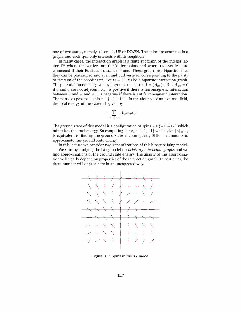
one of two states, namely `1 or ´1, UP or DOWN. The spins are arranged in agraph, and each spin only interacts with its neighbors.

In many cases, the interaction graph is a finite subgraph of the integer lat-tice Zn where the vertices are the lattice points and where two vertices areconnected if their Euclidean distance is one. These graphs are bipartite sincethey can be partitioned into even and odd vertices, corresponding to the parityof the sum of the coordinates. Let G “ pV,Eq be a bipartite interaction graph.The potential function is given by a symmetric matrix A “ pAuvq P SV . Auv “ 0if u and v are not adjacent, Auv is positive if there is ferromagnetic interactionbetween u and v, and Auv is negative if there is antiferromagnetic interaction.The particles possess a spin x P t´1,`1uV . In the absence of an external field,the total energy of the system is given by

´ÿ

tu,vuPE

Auvxuxv.

The ground state of this model is a configuration of spins x P t´1,`1uV whichminimizes the total energy. So computing the xu P t´1,`1u which give A8Ñ1

is equivalent to finding the ground state and computing SDP8Ñ1 amounts toapproximate this ground state energy.

In this lecture we consider two generalizations of this bipartite Ising model.We start by studying the Ising model for arbitrary interaction graphs and we

find approximations of the ground state energy. The quality of this approxima-tion will clearly depend on properties of the interaction graph. In particular, thetheta number will appear here in an unexpected way.

Figure 8.1: Spins in the XY model

127

Another generalization will be the consideration of more complicated spins.Instead of looking only at spins attaining the values ´1 and `1 as in the Isingmodel, the r-vector model considers spins which are vectors in the unit sphereSr´1 “ tx P Rr : x ¨ x “ 1u. The case r “ 1 corresponds to the Ising model, thecase r “ 2 to the XY model, the case r “ 3 to the Heisenberg model, and thecase r “ |V | to the Berlin-Kac spherical model. We will derive approximationsof ground state energies

´maxÿ

tu,vuPE

Au,vxu ¨ xv, for xu P Sr´1 and u P V

for fixed r and for bipartite graphs.In principle a mixture of both generalizations is possible. We do not give it

here as it would require adding even more technical details.

8.1 The Grothendieck constant of a graph

The Grothendieck constant of an undirected graph G “ pV,Eq is the smallestconstant1 KpGq “ K so that for every symmetric matrix A P SV the inequality

max

$

&

%

ÿ

tu,vuPE

Auvfu ¨ fv : fu P RV , u P V, fu “ 1

,

.

-

ď K max

$

&

%

ÿ

tu,vuPE

Auvxuxv : xu “ ˘1, u P V

,

.

-

holds true. The left hand side is the semidefinite relaxation of the right handside. Furthermore, the original Grothendieck constant which we studied in thelast lecture is equal to the supremum of KpGq over all bipartite graphs G; seeExercise 8.1 (a).

The following theorem gives a surprising connection between the Grothendieckconstant of a graph and the theta number.

Theorem 8.1.1. There is a constant C so that for any graph G we have

KpGq ď C lnϑpGq,

where ϑpGq is the theta number of the complementary graph of G.

The proof of this theorem will again be based on an approximation algo-rithm which performs randomized rounding of the solution of the semidefiniterelaxation.

1Do not confuse the KpGq with KG of the last lecture.

128

8.1.1 Randomized rounding by truncating

In the algorithm we use the constant M “ 3b

1` lnϑpGq. The meaning of itwill become clear when we analyze the algorithm.

1. Solve the semidefinite relaxation

Γmax “ max

$

&

%

ÿ

tu,vuPE

Auvfu ¨ fv : fu P RV , u P V, fu “ 1

,

.

-

2. Choose a random vector z “ pzuq P RV so that every entry zu is distributedindependently according to the standard normal distribution with mean 0and variance 1: zu „ Np0, 1q.

3. Round to real numbers yu “ z ¨ fu for all u P V .

4. Truncate yu by setting

xu “

"

yu if |yu| ďM ,0 otherwise

We denote by ∆ the optimal value of the ˘1-constrained problem

∆ “ max

$

&

%

ÿ

tu,vuPE

Auvxuxv : xu “ ˘1, u P V

,

.

-

.

Important note. The solution xu which the algorithm determines does notsatisfy the ˘1-constraint. It only lies in the interval r´M,M s by construction.However, it is easy to show (how? see Exercise 7.3 (b)) that

M2∆ “ max

$

&

%

ÿ

tu,vuPE

Auvxuxv : xu P r´M,M s, u P V

,

.

-

holds. Similarly,

Γmax “ max

$

&

%

ÿ

tu,vuPE

Auvfu ¨ fv : fu P RV , u P V, fu ď 1

,

.

-

In the remainder of this section we shall prove the theorem by giving anexplicit bound on the ratio Γmax∆.

129

8.1.2 Quality of expected solution

The expected quality of the solution xu isÿ

tu,vuPE

AuvErxuxvs

“ÿ

tu,vuPE

AuvpEryuyvs ´ Eryupyv ´ xvqs

´ Eryvpyu ´ xuqs ` Erpyu ´ xuqpyv ´ xvqsq

“ Γmax ´ E

»

–

ÿ

tu,vuPE

Auvppyupyv ´ xvq ` yvpyu ´ xuqq

fi

fl

` E

»

–

ÿ

tu,vuPE

Auvpyu ´ xuqpyv ´ xvq

fi

fl

(8.1)

because Eryuyvs “ fu ¨ fv (Exercise 8.1 (b)).

8.1.3 A useful lemma

To estimate the second and third summand in (8.1) we use the following lemma.

Lemma 8.1.2. Let Xu, Yu be random variables with u P V . Assume

ErX2us ď A and ErY 2

u s ď B.

Then,

E

»

–

ÿ

tu,vuPE

AuvpXuYv `XvYuq

fi

fl ď 2?ABpΓmax ´ Γminq,

where

Γmin “ min

$

&

%

ÿ

tu,vuPE

Auvfu ¨ fv : fu P RV , u P V, fu ď 1

,

.

-

.

Proof. If ErX2us ď 1, then

E

»

–

ÿ

tu,vuPE

AuvXuXv

fi

fl P rΓmin,Γmaxs. (8.2)

This follows from the fact we can write`

ErXuXvs˘

u,vPV“`

fu ¨ fv˘

u,vPV

because the matrix on the left hand side is positive semidefinite (Exercise 8.1(c)) and thus has a Cholesky factorization.

130

We introduce new variables Uu and Vu to be able to apply (8.2). The newvariables are

Uu “1

2

´

Xu?A` Yu

?B¯

, Vv “1

2

´

Xu?A´ Yu

?B¯

.

Then ErU2us ď 1 and ErV 2

u s ď 1 (verify it). So we can apply (8.2)

E

»

–

ÿ

tu,vuPE

AuvpXuYv `XvYuq

fi

fl

“ 2?AB

¨

˝E

»

–

ÿ

tu,vuPE

AuvUuUv

fi

fl´ E

»

–

ÿ

tu,vuPE

AuvVuVv

fi

fl

˛

‚

ď 2?ABpΓmax ´ Γminq.

8.1.4 Estimating A and B in the useful lemma

It is clear, that Ery2us “ 1. We find an upper bound for Erpyu ´ xuq2s in the

following lemma.

Lemma 8.1.3.

Erpyu ´ xuq2s “ 21?

2π

ż 8

M

t2e´t22dt ďMe´M

22.

Proof. The equation follows from the definition of yu and xu and the normaldistribution. The inequality is coming from the following simple but noteworthytrick to estimate the integrand by an expression which can be integrated:

t2e´t22 ď pt2 ` t´2qe´t

22.

Then,ż

pt2 ` t´2qe´t22dt “ ´

t2 ` 1

te´t

22 ` constant of integration,

and the lemma follows by

21?

2π

ż 8

M

t2e´t22dt ď

c

2

πpM ` 1Mqe´M

22 ďMe´M

22

because the fact M ě 2 implies thatc

2

πpM ` 1Mq ď

4

5pM ` 1Mq ďM.

131

8.1.5 Applying the useful lemma

In (8.1) we estimate the second summand by applying the useful lemma withXu “ yu, Yu “ yu ´ xu. We get

´E

»

–

ÿ

tu,vuPE

Auvppyupyv ´ xvq ` yvpyu ´ xuqq

fi

fl ě ´2a

Me´M22pΓmax ´ Γminq.

The third summand in (8.1) we estimate by applying the useful lemma withXu “ yu ´ xu, Yu “ ´pyu ´ xuq. We get

E

»

–

ÿ

tu,vuPE

Auvpyu ´ xuqpyv ´ xvq

fi

fl ě ´Me´M22pΓmax ´ Γminq.

Altogether,ÿ

tu,vuPE

AuvErxuxvs ě Γmax ´

´

2a

Me´M22 `Me´M22¯

pΓmax ´ Γminq.

8.1.6 Connection to the theta number

The connection to the theta number comes in the following lemma.

Lemma 8.1.4.Γmax ´ Γmin

Γmaxď ϑpGq.

Proof. Exercise 8.2.

In particular, we have

M ě M “ 3a

1` lnppΓmax ´ ΓminqΓmaxq.

Furthermore (lnx ď x´ 1),

M ď 3a

pΓmax ´ ΓminqΓmax

From this it follows that

Me´M22 ď Me´M

22 ď

1

10

ˆ

Γmax

Γmax ´ Γmin

˙2

.

So,ÿ

tu,vuPE

AuvErxuxvs ě Γmax ´2?

10Γmax ´

1

10

Γmax

Γmax ´ ΓminΓmax,

since Γmax ´ Γmin ě Γmax this leads toÿ

tu,vuPE

AuvErxuxvs ě1

4Γmax.

132

Finally we can put everything together: There is a positive constant C (which isnot difficult to estimate) so that

∆ ě1

M2

ÿ

tu,vuPE

AuvErxuxvs ě1

C lnϑpGqΓmax,

which finishes the proof of Theorem 8.1.1.

8.2 Higher rank Grothendieck inequality

Now we model finding ground states in the r-vector model. Given positiveintegers m, n, r and a matrix A “ pAijq P Rmˆn, the Grothendieck problem withrank-r-constraint is defined as

SDPrpAq “ max

" mÿ

i“1

nÿ

j“1

Aij xi ¨ yj : x1, . . . , xm P Sr´1, y1, . . . , yn P S

r´1

*

,

where Sr´1 “ tx P Rr : x ¨ x “ 1u is the unit sphere; the inner product matrixof the vectors x1, . . . , xm, y1, . . . , yn has rank at most r. When r “ 1, thenSDP1pAq “ A8Ñ1 because S0 “ t´1,`1u.

When r is a constant that does not depend on the matrix size m, n thereis no polynomial-time algorithm known which solves SDPr. However, it is notknown if the problem SDPr is NP-hard when r ě 2. On the other hand thesemidefinite relaxation of SDPrpAq defined by

SDPm`npAq “ max

" mÿ

i“1

nÿ

j“1

Aij ui ¨ vj : u1, . . . , um, v1, . . . , vn P Sm`n´1

*

can be computed in polynomial time using semidefinite programming.

Theorem 8.2.1. For all matrices A P Rmˆn we have

SDPrpAq ď SDPm`npAq ď1

2γprq ´ 1SDPrpAq,

where

γprq “2

r

ˆ

Γppr ` 1q2q

Γpr2q

˙2

,

and where Γ is the usual Gamma function, which is the extension of the factorialfunction.

The first three values of 12γprq´1 are:

1

2γp1q ´ 1“

1

4π ´ 1“ 3.65979 . . . ,

1

2γp2q ´ 1“

1

π2´ 1“ 1.75193 . . . ,

1

2γp3q ´ 1“

1

16p3πq ´ 1“ 1.43337 . . .

133

For r Ñ 8 the values 12γprq´1 converge to 1. In particular, the proof of the

theorem gives another proof of the original Grothendieck’s inequality albeit witha worse constant KG ď

14π´1 .

8.2.1 Randomized rounding by projecting

The approximation algorithm which we use to prove the theorem is the follow-ing three-step process.

1. By solving SDPm`npAqwe obtain the vectors u1, . . . , um, v1, . . . , vn P Sm`n´1.

2. Choose Z “ pZijq P Rrˆpm`nq so that every matrix entry Zij is distributedindependently according to the standard normal distribution with mean 0and variance 1: Zij „ Np0, 1q.

3. Project xi “ ZuiZui P Sr´1 with i “ 1, . . . ,m, and yj “ ZvjZvj P

Sr´1 with j “ 1, . . . , n.

8.2.2 Extension of Grothendieck’s identity

The quality of the feasible solution x1, . . . , xm, y1, . . . , yn for SDPr is measuredby the expectation

SDPrpAq ě E„ mÿ

i“1

nÿ

j“1

Aij xi ¨ yj

.

Lemma 8.2.2. Let u, v be unit vectors in Rm`n and let Z P Rrˆpm`nq be a ran-dom matrix whose entries are distributed independently according to the standardnormal distribution with mean 0 and variance 1. Then,

E„

Zu

Zu¨Zv

Zv

“2

r

ˆ

Γppr ` 1q2q

Γpr2q

˙2 8ÿ

k“0

p1 ¨ 3 ¨ ¨ ¨ p2k ´ 1qq2

p2 ¨ 4 ¨ ¨ ¨ 2kqppr ` 2q ¨ pr ` 4q ¨ ¨ ¨ pr ` 2kqqpu ¨ vq2k`1.

The case r “ 1 specializes to Grothendieck’s identity from the previous chap-ter:

ErsignpZuqsignpZvqs “2

πarcsinpu ¨ vq

“2

π

ˆ

u ¨ v `

ˆ

1

2

˙

pu ¨ vq3

3`

ˆ

1 ¨ 3

2 ¨ 4

˙

pu ¨ vq5

5` ¨ ¨ ¨

˙

.

The proof of Lemma 8.2.2 requires quite some integration. The computationstarts of by

E„

Zu

Zu¨Zv

Zv

“ p2πa

1´ t2q´rż

Rr

ż

Rr

x

x¨y

yexp

ˆ

´x ¨ x´ 2tx ¨ y ` y ¨ y

2p1´ t2q

˙

dxdy,

134

where t “ u ¨v. We will omit the tedious calculation here. For those who cannotresist a definite integral (like G.H. Hardy): it can be found in [4].

The only three facts which will be important is that the power series expan-sion

E„

Zu

Zu¨Zv

Zv

“

8ÿ

k“0

f2k`1pu ¨ vq2k`1

has the following three properties:

1. the leading coefficient f1 equals γprq

2. all coefficients f2k`1 are nonnegative

3.ř8

k“0 f2k`1 “ 1.

8.2.3 Proof of the theorem

Now we have

E„ mÿ

i“1

nÿ

j“1

Aij xi ¨ yj

“

mÿ

i“1

nÿ

j“1

AijE„

ZuiZui

¨ZvjZvj

“ f1

mÿ

i“1

nÿ

j“1

Aijui ¨ vj `mÿ

i“1

nÿ

j“1

Aij

8ÿ

k“1

f2k`1pui ¨ vjq2k`1.

The first summand equals f1SDPm`npAq. The second summand is bounded inabsolute value by p1´ f1qSDPm`npAq as you will prove in Exercise 8.1 (d).

Thus for the second sum we have

mÿ

i“1

nÿ

j“1

Aij

8ÿ

k“1

f2k`1pui ¨ vjq2k`1 ě pf1 ´ 1qSDPm`npAq,

which finishes the proof.

8.3 Further reading

Section 8.1: The result is from [1] and the presentation of the proof is closelyfollowing Chapter 10 of the book Approximation Algorithms and SemidefiniteProgramming of Gartner and Matousek, which mostly follows K. Makarychev’sthesis.

Section 8.2: The proof is from [3] and it follows the idea of Alon and Naor[2, Section 4] which in turn relies on ideas of Rietz.

More on the definite integral: When working with power series expansionsit is sometimes useful to use hypergeometric functions for this. For instance we

135

have

8ÿ

k“0

p1 ¨ 3 ¨ ¨ ¨ p2k ´ 1qq2

p2 ¨ 4 ¨ ¨ ¨ 2kqppr ` 2q ¨ pr ` 4q ¨ ¨ ¨ pr ` 2kqqpu ¨ vq2k`1

“ pu ¨ vq 2F1

ˆ

12, 12r2` 1

; pu ¨ vq2˙

,

where 2F1 is a hypergeometric function. Hypergeometric functions are a clas-sical subject in mathematics. In fact, many (all?) functions you know, are hy-pergeometric functions. However the topic of hypergeometric functions seemssomehow to be too classical for many modern universities.In case you want to know more about them: The book ”A=B” by Petkovsek,Wilf and Zeilberger

http://www.math.upenn.edu/~wilf/AeqB.html

is a good start.

8.4 Exercises

8.1** (a) Why does Theorem 8.1.1 give a proof of the original Grothendieckinequality? Which explicit upper bound for KG does it provide? (De-termine a concrete number.)

(b) Show that Eryuyvs “ fu ¨ fv holds.

(c) Prove that the matrix`

ErXuXvs˘

u,vPV

is positive semidefinite.

(d) Show thatˇ

ˇ

ˇ

ˇ

ˇ

mÿ

i“1

nÿ

j“1

Aij

8ÿ

k“1

f2k`1pui ¨ vjq2k`1

ˇ

ˇ

ˇ

ˇ

ˇ

ď p1´ f1qSDPm`npAq.

8.2 Let G “ pV,Eq be a graph. A vector k-coloring of G is a collection of unitvectors fu P RV so that

fu ¨ fv “ ´1

k ´ 1if tu, vu P E.

(a) Show that if G is colorable with k colors, then it also has a vectork-coloring.

(b) Find a connection between vector k-colorings and the theta number.

(c) Prove Lemma 8.1.4.

136

http://www.math.upenn.edu/~wilf/AeqB.html

BIBLIOGRAPHY

[1] N. Alon, K. Makarychev, Y. Makarychev, A. Naor, Quadratic forms ongraphs, Invent. Math. 163 (2006), 499–522.

[2] N. Alon, A. Naor, Approximating the cut-norm via Grothendieck’s inequal-ity, SIAM J. Comp. 35 (2006), 787–803.

[3] J. Briet, F.M. de Oliveira Filho, F. Vallentin, The Grothendieck problemwith rank constraint, pp. 111–113 in Proceedings of the 19th Symposiumon Mathematical Theory of Networks and Systems, 2010

[4] J. Briet, F.M. de Oliveira Filho, F. Vallentin, Grothendieck inequali-ties for semidefinite programs with rank constraint, arXiv:1011.1754v1[math.OC]


137


Part III

Applications in geometry

138

CHAPTER 9

OPTIMIZING WITHELLIPSOIDS ANDDETERMINANTS

What is an ellipsoid?

There are two convenient ways to represent an ellipsoid.

1. We can define ellipsoids explicitly as the image of the unit ball under aninvertible affine transformation

EA,c “ tAx` c : x P Bu, where B “ tx P Rn : x ď 1u,

is the unit ball, where A P Rnˆn is an invertible matrix, and where c P Rn is atranslation vector.

From linear algebra it is known that every invertible matrix A has a factor-ization of the form A “ XP where X P Sną0 is a positive definite matrix andP P Opnq is an orthogonal matrix. So we may assume in the following that thematrix A which defines the ellipsoid EA,c is a positive definite matrix.

In fact one can find this factorization (also called polar factorization) fromthe singular value decomposition of A

A “ UTΣV, U, V P Opnq, Σ “ diagpσ1, . . . , σnq,

where σi ě 0 are the singular values of A. Then,

A “ XP with X “ UTΣU, P “ UTV.

139

The singular values of A are at the same time the lengths of the semiaxis of theellipsoid EA,c.

The volume of the ellipsoid equals

vol EA,c “ detA volB where volB “πn2

Γpn2` 1q.

2. We can define ellipsoids implicitly by a strictly convex quadratic inequal-ity: Let A P Sną0 be a positive definite matrix, then

EA,c “ tAx` c : x ď 1u

“ tx` c : A´1x ď 1u

“

x P Rn : px´ cqTA´2px´ cq ď 1(

.

Ellipsoids are important geometric objects partially due to their simple de-scriptions. They can be used for instance to approximate other more compli-cated convex sets. In this lecture we will use ellipsoids to approximate poly-topes. In particular we will answer the questions:

• Inner approximation: How can we determine an ellipsoid contained in apolytope which has largest volume?

• Outer approximation: How can we determine an ellipsoid containing apolytope which has smallest volume?

• Can we estimate the quality of this inner and of this outer approximation?

9.1 Determinant maximization problems

To be able to maximize the volume of ellipsoids we want to maximize the de-terminant of positive definite matrices. In the next section we will see that thelogarithm of the determinant is a concave function so that determinant maxi-mization can be dealt with tools from convex optimization.

In fact one can reformulate determinant maximization problems as semidef-inite programs but we will not do this here; dealing directly with determinantmaximization problem is generally easier and more efficient.

Here we give the primal-dual pair of a determinant maximization problemtogether with the corresponding duality theory. All in all it is very similar tosemidefinite programming, only the objective function is not linear.

The primal determinant maximization problem is defined as

sup n` xC,Xy ` ln detX

X P Sną0

xAj , Xy “ bj , j “ 1, . . . ,m,

140

and its dual is

inf bTy ´ ln det

˜

mÿ

j“1

yjAj ´ C

¸

y P Rmmÿ

j“1

yjAj ´ C P Sną0

We have statements for weak duality and strong duality, which are very sim-ilar to Theorem 3.4.1. A slight difference is complementary slackness and theoptimality criterion. The optimality criterion says: Suppose that X is feasiblefor the primal, y is feasible for the dual and the equality

X

˜

mÿ

j“1

yjAj ´ C

¸

“ In

holds. Then X and y are both optimal (see Exercise 9.1 (a)).In many cases it is useful to combine determinant maximization problems

with linear conic programs. In these cases we want to work with the followingprimal-dual pair.

Primal:

sup n` xC,Xy ` ln detX ` cTx

X P Sną0

x P K

xAj , Xy ` aTj x “ bj , j “ 1, . . . ,m

Dual:

inf bTy ´ ln det

˜

mÿ

i“1

yjAj ´ C

¸

y P Rmmÿ

j“1

yjAj ´ C P Sną0

mÿ

j“1

yjaj ´ c P K˚

9.2 Convex spectral functions

In this section we shall prove that the function X ÞÑ ´ ln detX is a (strictly)convex function. For this we will give two proofs. One simple adhoc proof andone which is conceptual. The second proof will characterize all convex functionson symmetric matrices which only depend on the eigenvalues.

141

9.2.1 Minkowski’s determinant inequality

Theorem 9.2.1. The function

F : Sną0 Ñ R, X ÞÑ ´ ln detX

is a strictly convex function on the set of positive definite matrices.

Proof. It suffices to show that the function X ÞÑ ´ ln detX is strictly convex onany line segment

rX,Y s “ ttX ` p1´ tqY : t P r0, 1s, X ‰ Y u

in Sną0. Therefore, we compute the second derivative of the one-dimensionalfunction fptq “ ´ ln detptX`p1´ tqY q and see that it is always strictly positive:From linear algebra we know that there is a matrix T with determinant 1 whoseinverse simultaneously diagonalizes X and Y . Hence,

X “ TT diagpx1, . . . , xnqT and Y “ TT diagpy1, . . . , ynqT

and

fptq “ ´ lnpy1 ` tpx1 ´ y1qq ´ ¨ ¨ ¨ ´ lnpyn ` tpxn ´ ynqq,

Bf

Btptq “ ´

x1 ´ y1y1 ` tpx1 ´ y1q

´ ¨ ¨ ¨ ´xn ´ yn

yn ` tpxn ´ ynq,

B2f

Bt2ptq “

ˆ

x1 ´ y1y1 ` tpx1 ´ y1q

˙2

` ¨ ¨ ¨ `

ˆ

xn ´ ynyn ` tpxn ´ ynq

˙2

ą 0.

With the same argument we can derive Minkowski’s determinental inequality:

pdetpX ` Y qq1n ě pdetXq1n ` pdetY q1n

which holds for all X,Y P Sną0.Geometrically, this means that in the cone of positive semidefinite matrices,

the set of matrices having determinant greater or equal than a given constant isa convex set.

9.2.2 Davis’ characterization of convex spectral functions

The function F pXq “ ´ ln detX is an example of a convex spectral function.

Definition 9.2.2. A convex spectral function is a convex function

F : Sn Ñ RY t8u

where F pXq only depends on the spectrum (the collection of the eigenvalues λ1pXq,. . . , λnpXq) of the matrix X. In other words, by the spectral theorem,

F pXq “ fpAXATq for all A P Opnq.

Hence, there is a function f : Rn Ñ R Y t8u which defines F by the followingequation

F pXq “ fpλ1pXq, . . . , λnpXqq.

142

Note that this implies that the function f is symmetric, i.e. its value stays thesame if we permute its n arguments; it is invariant under permutation of thevariables.

In our example

fpλ1, . . . , λnq “

$

&

%

´ lnnś

i“1

λi if all λi ą 0,

8 otherwise.

The following theorem is due to Davis (1957). It gives a complete charac-terization of convex spectral functions.

Theorem 9.2.3. A function F : Sn Ñ R Y t8u is a convex spectral function ifand only if the function f : Rn Ñ RY t8u defined by

F pXq “ fpλ1pXq, . . . , λnpXqq

is symmetric and convex. In particular,

F pXq “ maxAPOpnq

fppAXATq11, . . . , pAXATqnnq

holds.

Proof. One implication follows without any work.Let F be a convex spectral function. Then f is symmetric by definition. It

is convex since F and f “coincide” on diagonal matrices. Let Λ “ pλ1, . . . , λnq,M “ pµ1, . . . , µnq and t P r0, 1s be given. Then

fptΛ` p1´ tqMq “ F pdiagptΛ` p1´ tqMqq

“ F ptdiagpΛq ` p1´ tqdiagpMqq

ď tF pdiagpΛqq ` p1´ tqF pdiagpMqq

“ tfpΛq ` p1´ tqfpMq.

The proof of the other implication is more interesting. It is an application ofBirkhoff’s theorem (cf. Chapter 1.7.3), see also the geometric interpretation atthe end of this section.

If we show that

F pXq “ maxAPOpnq

fppAXATq11, . . . , pAXATqnnq

holds, then it follows that F is convex because it is a maximum of a family ofconvex functions.

For this consider the spectral decomposition of X

X “

nÿ

j“1

λjujuTj .

143

with orthonormal basis u1, . . . , un. If we assemble these vectors as row vectorsin the orthogonal matrix A we see that

fppAXATq11, . . . , pAXATqnnq “ fpλ1, . . . , λnq “ F pXq

holds. Thus,

F pXq ď maxAPOpnq

fppAXATq11, . . . , pAXATqnnq.

The other inequality. For A P Opnq define Y “ AXAT. Then,

Yii “ eTi Y ei “ eTi

˜

nÿ

j“1

λjAujpAujqT

¸

ei “nÿ

j“1

λjppAujqTeiq

2.

Here is the trick: The matrix

S “ pSijq1ďi,jďn with Sij “ ppAujqTeiq

2

is doubly stochastic (why?). So by Birkhoff’s theorem S is a convex combinationof permutation matrices Pσ.

S “ÿ

σPSn

µσPσ, where µσ ě 0,

ÿ

σPSn

µσ “ 1.

Hence by the convexity and the symmetry of f , we have

fpY11, . . . , Ynnq “ f

˜

ÿ

σPSn

µσ

nÿ

j“1

Pσ1jλj , . . . ,ÿ

σPSn

µσ

nÿ

j“1

Pσnjλj

¸

ďÿ

σPSn

µσf

˜

nÿ

j“1

Pσ1jλj , . . . ,nÿ

j“1

Pσnjλj

¸

“ÿ

σPSn

µσfpλσ´1p1q, . . . , λσ´1pnqq

“ÿ

σPSn

µσfpλ1, . . . , λnq

“ fpλ1, . . . , λnq

“ F pXq.

Hence, for all A P Opnq

fppAXATq11, . . . , pAXATqnnq ď F pXq,

and the theorem is proved.

We conclude this excursion with a geometric observation which unifiessome of our previous considerations. If we project matrices in the Schur-Horn orbitope of X which is defined by

convtAXAT : A P Opnqu

144

on the diagonal elements, then we get the permutahedron given by theeigenvalues λ1, . . . , λn of X which is defined as

convtpλσp1q, . . . , λσpnqq : σ P Snu.

From this the Hoffman-Wielandt inequality and the characterization ofDavis follow.

Another side remark: Davis’ characterization together with Fan’s theo-rem (Theorem 2.2.2) can be used to determine an explicit linear matrixinequality modeling the condition F pXq ď t for many functions F . SeeBen-Tal, Nemirovski [3][Proposition 4.2.1] for the complete statement.A similar argument also works for functions depending only on singularvalues.

9.3 Approximating polytopes by ellipsoids

Now we are ready to describe how ellipsoids can be used to approximate poly-topes.

Recall that one can represent a polytope in two ways. Either as a convexhull of finitely many points

P “ convtx1, . . . , xNu P Rn,

or as a bounded intersection of finitely many halfspaces

P “ tx P Rn : aT1x ď b1, . . . , aTmx ď bmu.

The first representation, also called the V-representation, is an explicit pa-rameterization whereas the second one, also called the H-representation, isimplicit. In general it is computationally demanding to transform one represen-tation into the other.

9.3.1 Inner approximation

To formulate the condition that an ellipsoid EA,c is contained in a polytope Pwe will use the explicit representation of the ellipsoid and the implicit represen-tation of the polytope.

Proposition 9.3.1. The ellipsoid

EA,c “ tAx` c : x ď 1u

is contained in the polytope

P “ tx P Rn : aT1x ď b1, . . . , aTmx ď bmu

if and only if the inequalityAai ď bi ´ a

Ti c

holds for all i “ 1, . . . ,m.

145

Proof. We have

aTi pAx` cq ď bi @x P Rn : x ď 1

ðñ maxx:xď1

pAaiqTx ď bi ´ a

Ti c

ðñ Aai ď bi ´ aTi c,

because by the Cauchy-Schwarz inequality maxx:xď1pAaiqTx “ Aai.

The inequality Aai ď bi ´ aTi c can be directly modeled by a second ordercone programming constraint or, using the Schur complement, by a semidefiniteconstraint.

9.3.2 Outer approximation

To formulate the condition that an ellipsoid EA,c is containing a polytope P wewill use the implicit representation of the ellipsoid and the explicit representa-tion of the polytope.

Proposition 9.3.2. The ellipsoid

EA´12,c “ tx P Rn : px´ cqTApx´ cq ď 1u

contains the polytopeP “ convtx1, . . . , xNu

if and only if the matrixˆ

s dT

d A

˙

is positive semidefinite with Ac “ d and the inequality

xTi Axi ´ 2xTi d` s ď 1

holds for all i “ 1, . . . , N .

Proof. The point xi lies in the ellipsoid EA´12,c if and only if

pxi ´ cqTApxi ´ cq ď 1

ðñ xTi Axi ´ 2xTi Ac` cTAc ď 1

ðñ xTi Axi ´ 2xTi d` dTA´1d ď 1

ðñ xTi Axi ´ 2xTi d` s ď 1, where s ě dTA´1d.

Because the matrix A is positive definite we can express s ě dTA´1d using theSchur complement as

ˆ

s dT

d A

˙

ľ 0.

146

The constraintxTi Axi ´ 2xTi d` s ď 1

can be expressed by the linear matrix inequalityBˆ

1 xTixi xix

Ti

˙

,

ˆ

s dT

d A

˙F

ď 1.

9.4 The Lowner-John ellipsoids

Using Proposition 9.3.1 and Proposition 9.3.2 one can find the ellipsoid oflargest volume contained in a polytope P as well as the ellipsoid of smallest vol-ume containing P by solving determinant maximization problems. In both casesone maximizes the logarithm of the determinant of A. Because the logarithm ofthe determinant is a strictly concave function both optimization problems havea unique solution. The ellipsoids are called the Lowner-John ellipsoids1 of P .Notation: EinpP q for the ellipsoid giving the optimal inner approximation of Pand EoutpP q for the ellipsoid giving the optimal outer approximation of P .

The following theorem can be traced back to John (1948). Historically, it isconsidered to be one of the first theorems involving an optimality condition fornonlinear optimization.

Theorem 9.4.1. (a) Let P be a polytope. The Lowner-John ellipsoid EoutpP q isequal to the unit ball if and only if P is contained in the unit ball and thereis are positive numbers λ1, . . . , λN and vertices x1, . . . , xN of P having unitlength so that

Nÿ

i“1

λixi “ 0 andNÿ

i“1

λixixTi “ In

holds.

(b) Let P be a polytope. The Lowner-John ellipsoid EinpP q is equal to the unitball if and only if P is containing the unit ball and if there are unit vectorsx1, . . . , xN on the boundary of P and there are positive numbers λ1, . . . , λNso that

Nÿ

i“1

λixi “ 0 andNÿ

i“1

λixixTi “ In

holds.

Before we give the proof we comment on the optimality conditions. Thefirst equality makes sure that not all the vectors x1, . . . xN lie on one side ofthe sphere. The second equality shows that the vectors behave similar to an

1In the literature the terminology seems to differ from author to author.

147

orthonormal basis in the sense that we can compute the inner product of twovectors x and y by

xTy “Nÿ

i“1

λipxTi xqpx

Ti yq.

Proof. Statement (a) follows from the optimality conditions of the underlyingdeterminant maximization problem. See Exercise 9.1 (b).

Statement (b) follows from (a) by polarity:

Let C Ď Rn be a convex body. Its polar body C˚ is

C˚ “ tx P Rn : xTy ď 1 for all y P Cu.

The unit ball is self-polar, B˚ “ B. Furthermore, for every ellipsoid E we have

vol E vol E˚ ě pvolBq2,

because direct verification yields

pEA,cq˚ “ EA1,c1 with A1 “

ˆ

ATA

p1` 14c

TpATAq´1cq

˙´12

, c1 “ ´1

2pATAq´1c,

and sodetAdetA1 ě 1.

Let P be a polytope and assume that EinpP q “ B. We will now prove bycontradiction that B “ EoutpP˚q. For suppose not. Then the volume of EoutpP˚qis strictly smaller than the volume of B since P˚ Ď B. However, by taking thepolar again we have

EoutpP˚q˚ Ď P,

and vol EoutpP˚q˚ ą volpBq a contradiction. So by (a) we have for verticesx1, . . . , xN of P , which are of unit length, the conditions

Nÿ

i“1

λixi “ 0 andNÿ

i“1

λixixTi “ In,

for positive λ1, . . . , λN . Then the unit vectors xi also lie on the boundary of thepolytope P because

P “ pP˚q˚ “ tx P Rn : xTi x ď 1, i “ 1, . . . , Nu.

Now letEinpP q “ tx P Rn : px´ cqTA´2px´ cq ď 1u

be the optimal inner approximation of P . We want to derive from the optimalityconditions that detA ď 1 holds.

148

First we realize that the second optimality condition implies that the equa-tion

řNi“1 λi “ n holds; simply take the trace.

The pointsyi “ c` pxTi A

2xiq´12A2xi

lie in EinpP q and so yTi xi ď 1 holds because this inequality determines a sup-porting hyperplanes of P . Then,

n ěNÿ

i“1

λiyTi xi “

Nÿ

i“1

λipxTi A

2xiq12

where we used the first equality when simplifyingřNi“1 λic

Txi “ 0. The traceof A can be estimated by using the second equality

xA, Iny “@

A,Nÿ

i“1

λixixTi

D

“

Nÿ

i“1

λixTi Axi ď

Nÿ

i“1

λipxTi A

2xiq12 ď n,

where we used in the first inequality the spectral factorization of A “ PTDP ,with orthogonal matrix P and diagonal matrix D, together with the Cauchy-Schwarz inequality

pxTi PTDqpPxiq ď px

Ti P

TD2Pxiq12ppPxiq

TPxiq12 “ pxTi P

TD2Pxiq12.

Now we finish the proof by realizing that (lnx ď x´ 1)

ln detA ď TrpAq ´ n ď 0,

and so detA ď 1.

This optimality condition is helpful in surprisingly many situation. For ex-ample one can use them to prove an estimate on the quality of the inner andouter approximation.

Corollary 9.4.2. Let P Ď Rn be an n-dimensional polytope, then there are invert-ible affine transformations Tin and Tout so that

B “ TinEinpP q Ď TinP Ď nTinEinpP q “ nB

and1

nB “

1

nToutEoutpP q Ď ToutP Ď ToutEoutpP q “ B

holds.

Proof. We only prove the first statement, the second follows again by polarity.It is clear that we can map EinpP q to the unit ball by an invertible affine

transformation. So we can use the equations

Nÿ

i“1

λixi “ 0 andNÿ

i“1

λixixTi “ In

149

to show TinP Ď nEinpP q. By taking the trace on both sides of the secondequations we also have

Nÿ

i“1

λi “ n.

The supporting hyperplane through the boundary point xi of P is orthogonalthe unit vector xi (draw a figure). Hence,

B Ď P Ď Q “ tx P Rn : xTi x ď 1, i “ 1, . . . , Nu.

Let x be in Q, then because xTxi P r´x, 1s we have

0 ďNÿ

i“1

λip1´ xTxiqpx ` x

Txiq

“ xNÿ

i“1

λi ` p1´ xqNÿ

i“1

λixTxi ´

Nÿ

i“1

λipxTxiq

2

“ xn` 0´ x2,

and so x ď n.

If P is centrally symmetric, i.e. P “ ´P , then in the above inequalities ncan be replaced by

?n. See Exercise 9.1 (c).

Another nice mathematical application of the uniqueness Lowner-John el-lipsoids is the following.

Proposition 9.4.3. Let P be a polytope and consider the group G of all affinetransformations which map P into itself. Then there is an affine transformation Tso that TGT´1 is a subgroup of the orthogonal group.

Proof. Since the volume is invariant under affine transformations with determi-nant equal to 1 or ´1 (only those affine transformations can be in G) and sincethe Lowner-John ellipsoid is the unique maximum volume ellipsoid containedin a polytope we have

AEinpP q “ EinpAP q “ EinpP q

for all A P G.Let T be the affine transformation which maps the Lowner-John ellipsoid

EinpP q to the unit ball B. Then for every A P G

TAT´1B “ TAEinpP q “ TEinpP q “ B.

So TAT´1 leaves the unit ball invariant, hence it is an orthogonal transforma-tion.

150

9.5 Further reading

Many examples of determinant maximization problems are in Vandenberghe,Boyd and Wu [5]. They treat matrix completion problems, risk-averse linearestimation, experimental design, maximum likelihood estimation of structuredcovariance matrices, and Gaussian channel capacity. Next to this, they also de-velop the duality theory and an interior point algorithm for determinant maxi-mization problems.

For more information on convex spectral functions and general eigenvalueoptimization problems the survey [4] by Lewis is a good start.

Many more examples of computing ellipsoidal approximations are in thebook [3][Chapter 4.9], especially ellipsoidal approximations of unions and in-tersections of ellipsoids and approximating sums of ellipsoids.

The Lowner-John ellipsoid is an important and useful concept in geometry,optimization, and functional analysis. For instance, Lenstra’s polynomial timealgorithm for solving integer programs in fixed dimension is based on it (seeLNMB course: Integer programming methods).

Another excellent and very elegant source on applications of the Lowner-John ellipsoid in geometry and functional analysis is by Ball [2]. He uses John’soptimality criterion to give a reverse isoperimetric inequality (the ratio betweensurface and volume is maximized by cubes) and to prove Dvoretsky’s theorem(high dimensional convex bodies have almost ellipsoidal slices). The proof ofthe second part of Theorem 9.4.1 (b) is from the beautiful note of Ball [1].

One general strategy when working with convex sets is to find an affinetransformation of the convex set so that the unit ball and the convex set areas close as possible. Here the notion of closeness depends of course on thequestion. In many cases these affine transformations can be found by solvingan optimization problem involving positive definite matrices.

9.6 Exercises

9.1** (a) Prove weak duality of determinant maximization problems: Let X bea solution of the primal and let y be a solution of the dual. Then,

bTy ´ ln det

˜

mÿ

j“1

yjAj ´ C

¸

´ pn` xC,Xy ` ln detXq ě 0.

Hint: lnx ď x´ 1.

(b) Prove Theorem 9.4.1 (a).

(c) Show the strengthening of Corollary 9.4.2

B “ TinEinpP q Ď TinP Ď?nTinEinpP q “

?nB

in the case of centrally symmetric polytopes P .

151

(d) Find a polytope P for which the inclusion

B Ď P Ď nB

cannot be improved. Find a centrally symmetric polytope for which

B Ď P Ď?nB

cannot be improved.

9.2 (a) Show that the sum of the largest k eigenvalues of a symmetric matrixis a convex spectral function.

(b) True or false: The second largest eigenvalue of a symmetric matrix isa convex spectral function.

9.3 Compute the gradient of the function

F : Sną0 Ñ R, X ÞÑ ´ ln detX.

152

BIBLIOGRAPHY

[1] K.M. Ball, Ellipsoids of maximal volume in convex bodies, GeometriaeDedicata 41 (1992), 241–250.

[2] K.M. Ball, An Elementary Introduction to Modern Convex Geometry, pp. 1–58 in: Flavors of Geometry (S. Levy (ed.)), Cambridge University Press,1997.

http://library.msri.org/books/Book31/files/ball.pdf


[4] A.S. Lewis, The mathematics of eigenvalue optimization, Math. Program.,Ser. B 97 (2003), 155–176.

http://people.orie.cornell.edu/~aslewis/publications/

03-mathematics.pdf

[5] L. Vandenberghe, S. Boyd, S.-P. Wu, Determinant Maximization with Lin-ear Matrix Inequality Constraints, SIAM Journal on Matrix Analysis andApplications 19 (1998), 499–533.

http://www.stanford.edu/~boyd/papers/maxdet.html

153

http://library.msri.org/books/Book31/files/ball.pdf

http://people.orie.cornell.edu/~aslewis/publications/03-mathematics.pdf

http://people.orie.cornell.edu/~aslewis/publications/03-mathematics.pdf

http://www.stanford.edu/~boyd/papers/maxdet.html

CHAPTER 10

EUCLIDEAN EMBEDDINGS:LOW DIMENSION

In many situations one is interested in finding solutions to semidefinite pro-grams having a small rank. For instance, if the semidefinite program arisesas relaxation of a combinatorial optimization problem (like max-cut or maxclique), then its rank one solutions correspond to the solutions of the underly-ing combinatorial problem. Finding an embedding of a weighted graph in theEuclidean space of dimension d, or finding a sum of squares decomposition ofa polynomial with d squares, amounts to finding a solution of rank at most dto some semidefinite program. As another example, the minimum dimension ofan orthonormal representation of a graph G “ pV,Eq (introduced in Chapter 6)is the minimum rank of a positive semidefinite matrix X satisfying Xij “ 0 forall non-edges.

This chapter is organized as follows. First we show some upper bounds onthe rank of solutions to semidefinite programs. For this we have to look intothe geometry of the faces of the cone of positive semidefinite matrices. Then wediscuss several applications: Euclidean embeddings of weighted graphs, hiddenconvexity results for images of quadratic maps, and the S-lemma which dealswith quadratic inequalities. We also discuss complexity issues related to theproblem of determining the smallest possible rank of solutions to semidefiniteprograms.

154

10.1 Geometry of the positive semidefinite cone

10.1.1 Faces of convex sets

We begin with some preliminary facts about faces of convex sets which we willuse to study the faces of the positive semidefinite cone Snľ0.

Let K be a convex set in Rn. A set F Ď K is called a face of K if for all x P Fthe following holds:

x “ ty ` p1´ tqz with t P p0, 1q, y, z P K ùñ y, z P F.

Clearly any intersection of faces is again a face. Hence, for x P K, the smallestface containing x is well defined (as the intersection of all the faces of K thatcontain x), let us denote it by FKpxq.

A point z P Rn is called a perturbation of x P K if x˘ εz P K for some ε ą 0;then the whole segment rx´ εz, x` εzs is contained in the face FKpxq.

Lemma 10.1.1. Given a convex set K and x P K, let FKpxq be the smallest faceof K containing x. The following properties hold.

(i) x belongs to the relative interior of FKpxq.

(ii) FKpxq is the unique face of K containing x in its relative interior.

Proof. (i) Assume for a contradiction that x R relint FKpxq. Then, by applyingthe separation theorem from Theorem 1.3.8 (i), there exists a hyperplane

Hc,γ “ ty : cTy “ γu

separating the two convex sets txu and FKpxq properly: There exist a nonzerovector c P Rn and γ P R such that

cTx ě γ, cTy ď γ @y P FKpxq, and FKpxq Ę Hc,γ .

Then the set FKpxq XHc,γ is a face of K, which contains x and is strictly con-tained in FKpxq (check it). This contradicts the fact that FKpxq is the smallestface containing x.

(ii) Let F be a face ofK containing x in its relative interior. Then FKpxq Ď F .To show the reverse inclusion, pick y P F , y ‰ x. As x lies in the relative interiorof F , Lemma 1.2.1 implies that there exists a point z P F and a scalar t P p0, 1qsuch that x “ ty ` p1 ´ tqz. As FKpxq is a face, we deduce that y, z P FKpxq.This shows that F Ď FKpxq.

Hence, x lies in the relative interior of K precisely when FKpxq “ K and xis an extreme point of K, i.e.,

x “ ty ` p1´ tqz with y, z P K and t P p0, 1q ùñ y “ z “ x,

precisely when FKpxq “ txu. Recall that if K does not contain a line then it hasat least one extreme point.

155

10.1.2 Faces of the positive semidefinite cone

Here we describe the faces of the positive semidefinite cone Snľ0. We show thateach face of Snľ0 can be identified to a smaller semidefinite cone Srľ0 for some0 ď r ď n.

Proposition 10.1.2. Let A P Snľ0, r “ rankpAq, and let F pAq “ FSnľ0pAq denote

the smallest face of Snľ0 containing A. Let u1, ¨ ¨ ¨ , un be an orthonormal set ofeigenvectors of A, where u1, ¨ ¨ ¨ , ur correspond to its nonzero eigenvalues, and letU (resp., U0) be the matrix with columns u1, ¨ ¨ ¨ , un (resp., u1, ¨ ¨ ¨ , ur). The map

φA : Sr Ñ Sn

Z ÞÑ U

ˆ

Z 00 0

˙

UT “ U0ZUT0

(10.1)

is a rank-preserving isometry, which identifies F pAq and Srľ0:

F pAq “ φpSrľ0q “

"

U

ˆ

Z 00 0

˙

UT “ U0ZUT0 : Z P Srľ0

*

.

Moreover, F pAq is given by

F pAq “ tX P Snľ0 : KerX Ě KerAu (10.2)

and its dimension is equal to`

r`12

˘

.

Proof. Set D “ diagpλ1, ¨ ¨ ¨ , λr, 0, ¨ ¨ ¨ , 0q P Snľ0, D0 “ diagpλ1, ¨ ¨ ¨ , λrq P Srą0,where λi is the eigenvalue for eigenvector ui, C “ diagp0, ¨ ¨ ¨ , 0, 1, ¨ ¨ ¨ , 1q PSnľ0, where the first r entries are 0 and the last n ´ r entries are 1. Finally,set Q “ UCUT “

řni“r`1 uiu

Ti . Then, A “ UDUT and xC,Dy “ 0. Moreover,

xQ,Ay “ 0, as the vectors ur`1, ¨ ¨ ¨ , un span the kernel of A.As Q ľ 0, the hyperplane

H “ tX P Sn : xQ,Xy “ 0u

is a supporting hyperplane for Snľ0 and the intersection

F “ Snľ0 XH “ tX P Snľ0 : xQ,Xy “ 0u

is a face of Snľ0 containing A. Moreover,

F “ tX P Snľ0 : KerX Ě KerAu.

Indeed, the condition xQ,Xy “ 0 readsř

i“r`1 uTi Xui “ 0. For X ľ 0,

uTi Xui ě 0 for all i, so that xQ,Xy “ 0 if and only if uTi Xui “ 0 or, equiv-alently, Xui “ 0 for all i P tr ` 1, ¨ ¨ ¨ , nu, i.e., KerA Ď KerX.

We now show that F “ F pAq. In view of Lemma 10.1.1, it suffices to showthat A lies in the relative interior of the face F .

156

For this, consider the linear bijection X ÞÑ Y “ UTXU . It maps Snľ0 ontoitself, Q onto C, and A onto D, and the face F onto the face

F 1 “ tUTXU : X P F u.

Hence, F 1 contains D and F 1 is equal to

F 1 “ tY P Snľ0 : xC, Y y “ 0u.

Any matrix Y P F 1 has its last n ´ r diagonal entries equal to 0 and thus it hasthe block form:

Y “

ˆ

Z 00 0

˙

where Z P Srľ0.

Therefore, the faces F 1 and F are given by

F 1 “

"ˆ

Z 00 0

˙

: Z P Srľ0

*

, F “

"

U

ˆ

Z 00 0

˙

UT : Z P Srľ0

*

.

As D0 ą 0, D0 lies in the interior of Srľ0. This implies that D lies in the relativeinterior of F 1 and, in turn, that A belongs to the relative interior of F . Thus,F “ F pAq.

Summarizing, we have shown that F pAq can be identified with Srľ0 via therank-preserving isometry:

Z ÞÑ Y “

ˆ

Z 00 0

˙

ÞÑ X “ UY UT

D0 ÞÑ D ÞÑ ASrľ0 Ñ F 1 Ñ F pAq

and the dimension of F is equal to dimSrľ0 “`

r`12

˘

.

As a direct application, the possible dimensions for the faces of the cone Snľ0

are`

r`12

˘

for r “ 0, 1, ¨ ¨ ¨ , n. Moreover there is a one-to-one correspondencebetween the lattice of faces of Snľ0 and the lattice of subspaces of Rn:

U subspace of Rn ÞÑ FU “ tX P Snľ0 : KerX Ě Uu, (10.3)

with U1 Ď U2 ðñ FU1 Ě FU2 .

10.1.3 Faces of spectrahedra

Consider an affine subpsace A in the space of symmetric matrices, of the form

A “ tX P Sn : xAj , Xy “ bj pj P rmsqu, (10.4)

whereA1, ¨ ¨ ¨ , Am are given symmetric matrices and b1, ¨ ¨ ¨ , bm are given scalars.The codimension of A is

codim A “ dimSn ´ dimA “ dimxA1, ¨ ¨ ¨ , Amy.

157

If we intersect the cone of positive semidefinite matrices with the affine spaceA, we obtain the convex set

K “ Snľ0 XA “ tX P Sn : X ľ 0, xAj , Xy “ bj pj P rmsqu. (10.5)

This is the feasible region of a typical semidefinite program (in standard primalform). Such a convex set is called a spectrahedron – this name is in the analogywith polyhedron, which corresponds to the feasible region of a linear programand spectra reflects the fact that the definition involves spectral properties ofmatrices.

An example of a spectrahedron is the elliptope

En “ tX P Snľ0 : Xii “ 1 @i P rnsu, (10.6)

which is the feasible region of the semidefinite relaxation for Max-Cut consid-ered in earlier chapters.

As an application of the description of the faces of the positive semidefinitecone in Proposition 10.1.2, we can describe the faces of K.

Proposition 10.1.3. Let K be the spectrahedron (15.2). Let A P K, r “ rankpAq,and let U,U0 be as in Proposition 10.1.2. Define the affine space in Sr:

AA “ tZ P Sr : xUT0 AjU0, Zy “ bj @j P rmsu, (10.7)

and the corresponding linear space:

LA “ tZ P Sr : xUT0 AjU0, Zy “ 0 @j P rmsu. (10.8)

The map φ from (10.1) identifies FKpAq and Srľ0 XAA: FKpAq “ φpSrľ0 XAAq.Moreover, FKpAq is given by

FKpAq “ tX P K : KerX Ě KerAu (10.9)

and its dimension is equal to

dimFKpAq “ dimAA “ˆ

r ` 1

2

˙

´ dimxUT0 AjU0 : j P rmsy. (10.10)

Finally, a matrix B P Sn is a perturbation of A if and only if B P U0LAUT0 .

Proof. As K “ Snľ0 X A, we have that FKpAq “ F pAq X A, where F pAq is thesmallest face of Snľ0 containing A, and (10.9) follows from (10.2). If X “ φpZqis the image of Z P Sr under the map φ from (10.1) then

xAj , Xy “ xUTAjU,U

TXUy “

B

UTAjU,

ˆ

Z 00 0

˙F

“ xUT0 AjU0, Zy.

Therefore, the face FKpAq is the image of Srľ0 X AA under the map φ and itsdimension is equal to dimAA. Finally, B is a perturbation of A if and only ifA˘ εB P FKpAq for some ε ą 0, which is equivalent to B P U0LAUT

0 using thedescription of FKpAq.

158

Corollary 10.1.4. Let K be defined as in (15.2). Let A P K and r “ rankpAq. IfA is an extreme point of K then

ˆ

r ` 1

2

˙

ď codim A ď m (10.11)

In particular, K contains a matrix A whose rank r satisfies

r ď´1`

?8m` 1

2. (10.12)

Proof. If A is an extreme point of K then dimFKpAq “ 0 and (15.15) followsdirectly from (10.10). As K contains no line, K has at least one extreme point.Now (10.12) follows directly from

`

r`12

˘

ď m for any matrix A which is anextreme point of K.

Remark 10.1.5. The codimension of the affine space AA can be expressed fromany Cholesky decomposition: A “WWT, where W P Rnˆr, by

codim AA “ dimxWAjWT : j P rmsy.

Indeed, the matrix P “ WTU0D´10 is nonsingular, since PTP “ D´1

0 using thefact that UT

0 U0 “ Ir. Moreover, WP “ U0, and thus

dimxWTAjW : j P rmsy “ dimxPTWTAjWP : j P rmsy “ dimxUT0 AjU0 : j P rmsy.

As an illustration, for the elliptope K “ En, if A P En is the Gram matrix of vectorsta1, ¨ ¨ ¨ , anu Ď Rk, then codim AA “ dimxa1a

T1 , ¨ ¨ ¨ , ana

Tny.

As an illustration we discuss a bit the geometry of the elliptope En. As adirect application of Corollary 10.1.4, we obtain the following bound for therank of extreme points:

Corollary 10.1.6. Any extreme point of En has rank r satisfying`

r`12

˘

ď n.

A matrix X P En has rank 1 if and only if it is of the form X “ xxT forsome x P t˘1un. Such matrix is also called a cut matrix (since it corresponds toa cut in the complete graph Kn). There are 2n´1 distinct cut matrices. They areextreme points of En and any two of them form an edge (face of dimension 1)of En. While for n ď 4, these are the only faces of dimension 1, the elliptopeEn for n ě 5 has faces of dimension 1 that are not an edge between two cutmatrices. You will see an example in Exercise 10.3.

Figure 10.1 shows the elliptope E3 (more precisely, its bijective image in R3

obtained by taking the upper triangular part ofX). Note the four corners, whichcorrespond to the four cuts of the graph K3. All the points on the boundary ofE3 - except those lying on an edge between two of the four corners – are extremepoints. For instance, the matrix

A “

¨

˝

1 0 1?

2

0 1 1?

2

1?

2 1?

2 1

˛

‚

is an extreme point of E3 (check it), with rank r “ 2.

159

Figure 10.1: The elliptope E3

10.1.4 Finding an extreme point in a spectrahedron

In order to find a matrix A in a spectrahedron K whose rank satisfies (10.12),it suffices to find an extreme point A of K. Algorithmically this can be done asfollows.

Suppose we have a matrix A P K with rank r. Observe that A is an extremepoint of K precisely when the linear space LA (in (10.8)) is reduced to the zeromatrix. Assume that A is not an extreme point of K. Pick a nonzero matrix C PLA, so that B “ U0CU

T0 is a nonzero perturbation of A. Hence A˘ tB ľ 0 for

some t ą 0. Moreover, at least one of the supremums: suptt ą 0 : A` tB ľ 0uand suptt ą 0 : A ´ tB ľ 0u is finite, since K contains no line. Say, the firstsupremum is finite, and compute the largest scalar t ą 0 for which A` tB ľ 0(this is a semidefinite program). Then the matrixA1 “ A`tB still belongs to theface FKpAq, but it now lies on its border (by the maximality of t). Therefore, A1

has a larger kernel: KerA1 Ą KerA, and thus a smaller rank: rankA1 ď rankA´1.Then iterate, replacing A by A1, until finding an extreme point of K.

Therefore, one can find an extreme point of K by solving at most n semidef-inite programs. However, finding the smallest possible rank of a matrix in K isa hard problem – see Proposition 10.2.4.

10.1.5 A refined bound on ranks of extreme points

The upper bound on the rank of an extreme point from Corollary 10.1.4 is tight– see Example 10.2.3 below. However, there is one special case when it can besharpened, as we explain here. Consider again the affine space A from (10.4)and the spectrahedron K “ Snľ0 XA. From Corollary 10.1.4, we know that anyextreme point A of K has rank r satisfying

ˆ

r ` 1

2

˙

ď codim A.

Hence, r ď s` 1 if codim A “`

s`22

˘

. Under some assumptions, Barvinok showsthat r ď s for at least one extreme point of K.

160

Proposition 10.1.7. Assume that K is nonempty bounded and codim A “`

s`22

˘

for some integer s ě 1 satisfying n ě s ` 2. Then there exists A P K withrank A ď s.

The proof uses the following topological result.

Theorem 10.1.8. Consider the projective space Pn´1, consisting of all lines in Rnpassing through the origin, and let Sn´1 be the unit sphere in Rn. For n ě 3 theredoes not exist a continuous map Φ : Sn´1 Ñ Pn´1 such that Φpxq ‰ Φpyq for alldistinct x, y P Sn´1.

The following lemma deals with the case n “ s`2, it is the core of the proofof Proposition 10.1.7.

Lemma 10.1.9. Let n “ s ` 2 with s ě 1 and let A Ď Ss`2 be an affine spacewith codim A “

`

s`22

˘

. If K “ Ss`2ľ0 XA is nonempty and bounded, then there is

a matrix A P K with rank A ď s.

Proof. Assume first that AXSs`2ą0 “ H. Then A lies in a hyperplane H support-

ing a proper face F of Ss`2ľ0 . (This can be checked using the separating theorem

from Theorem 1.3.8 (i).) By Proposition 10.1.2, F can be identified with Stľ0

for some t ď s` 1 and thus an extreme point of K has rank at most t´ 1 ď s.Suppose now that AX Ss`2

ą0 ‰ H. By (10.10), dimK “`

s`32

˘

´ codim A “s ` 2. Hence, K is a ps ` 2q-dimensional compact convex set, whose boundaryBK is (topologically) the sphere Ss`1. We now show that the boundary of Kcontains a matrix with rank at most s.

Clearly every matrix in BK has rank at most s ` 1. Suppose for a contra-diction that no matrix of BK has rank at most s. Then, each matrix X P BKhas rank s` 1 and thus its kernel KerX has dimension 1, it is a line though theorigin. We can define a continuous map Φ from BK to Ps`1 in the followingway: For each matrix X P BK, its image ΦpXq is the line KerX. The map Φis continuous (check it) from Ss`1 to Ps`1 with s ` 1 ě 2. Hence, applyingTheorem 10.1.8, we deduce that there are two distinct matrices X,X 1 P BKwith the same kernel: KerX “ KerX 1. Hence X and X 1 are two distinct pointslying in the same face of K: FKpXq “ FKpX

1q. Then this face has an extremepoint A, whose rank satisfies rankA ď rankX ´ 1 ď s.

We can now conclude the proof of Proposition 10.1.7.

Proof. (of Proposition 10.1.7). By Corollary 10.1.4 there exists a matrix A P Kwith rank A ď s ` 1. Pick a vector space U Ď KerA with codim U “ s ` 2. ByProposition 10.1.2, there is a rank-preserving isometry between FU and Ss`2

ľ0 .Moreover, A P FU XA. Hence the result follows by applying Lemma 10.1.9.

Example 10.1.10. Consider the three matrices

A “

ˆ

1 00 ´1

˙

, B “

ˆ

0 11 0

˙

, C “

ˆ

1 11 0

˙

161

and the affine space

A “ tX P S2 : xA,Xy “ 0, xB,Xy “ 0, xC,Xy “ 1u.

Then S2ľ0 X A “ tIu thus contains no rank 1 matrix, and codim A “ 3 “`

s`22

˘

with s “ 1. This example shows that the condition n ě s` 2 cannot be omitted inLemma 10.1.9.

Example 10.2.3 below shows that the assumption that K is bounded cannot beomitted as well.

10.2 Applications

10.2.1 Euclidean realizations of graphs

The graph realization problem can be stated as follows. Suppose we are givena graph G “ pV “ rns, Eq together with nonnegative edge weights w P RE`,viewed as ‘lengths’ assigned to the edges. We say that pG,wq is d-realizable ifone can place the nodes of G at points v1, ¨ ¨ ¨ , vn P Rd in such a way that theirEuclidean distances respect the given edge lengths:

Dv1, ¨ ¨ ¨ , vn P Rd vi ´ vj2 “ wij @ti, ju P E. (10.13)

(We use here the squares of the Euclidean distances as this makes the notationeasier). Moreover, pG,wq is realizable if it is d-realizable for some d ě 1. Indimension 3, the problem of testing d-realizability arises naturally in roboticsor computational chemistry (the given lengths represent some known distancesbetween the atoms of a molecule and one wants to reconstruct the moleculefrom these partial data).

Testing whether a weighted graph is realizable amounts to testing feasibilityof a semidefinite program:

Lemma 10.2.1. pG,wq is realizable if and only if the following semidefinite pro-gram (in matrix variable X P Sn):

Xii `Xjj ´ 2Xij “ wij @ti, ju P E, X ľ 0 (10.14)

has a feasible solution. Moreover, pG,wq is d-realizable if and only if the system(10.14) has a solution of rank at most d.

Proof. If v1, ¨ ¨ ¨ , vn P Rd is a realization of pG,wq, then their Gram matrix X “

pvTi vjq is a solution of rank at most d of (10.14). Conversely, if X is a solutionof (10.14) of rank ď d and v1, ¨ ¨ ¨ , vn P Rd is a Gram decomposition of X, thenthe vi’s form a d-realization of pG,wq.

As a direct application of Corollary 10.1.4, any realizable graph pG,wq isd-realizable in dimension d satisfying

ˆ

d` 1

2

˙

ď |E|, i.e., d ď´1`

a

8|E| ` 1

2. (10.15)

162

When G “ Kn is a complete graph, checking whether pKn, wq is d-realizableamounts to checking whether a suitable matrix is positive semidefinite and com-puting its rank:

Lemma 10.2.2. Consider the complete graph G “ Kn with edge weights w, anddefine the matrix X P Sn´1 by

Xii “ win pi P rn´ 1sq, Xij “win ` wjn ´ wij

2pi ‰ j P rn´ 1sq.

Then, pKn, wq is d-realizable if and only if X ľ 0 and rankX ď d.

Proof. The proof relies on the observation that if a set of vectors v1, ¨ ¨ ¨ , vn PRd satisfies (10.13), then one can translate it and thus assume without loss ofgenerality that vn “ 0.

Example 10.2.3. Consider the complete graph G “ Kn with weights wij “ 1 forall edges. Then pKn, wq is pn ´ 1q-realizable but it is not pn ´ 2q-realizable (easyto check using Lemma 10.2.2).

Hence, the upper bound (10.15) is tight on this example. This shows that thecondition that K is bounded cannot be omitted in Proposition 10.1.7. (Note thatthe set of feasible solutions to the program (10.14) is indeed not bounded).

On the other hand, for any fixed d ě 1, deciding whether a graph pG,wqis d-realizable is a hard problem. Therefore, deciding whether the semidefiniteprogram (10.14) has a solution of rank at most d is a hard problem.

We show this for d “ 1. Then there is a simple reduction from the partitionproblem: Decide whether a given sequence of integers a1, ¨ ¨ ¨ , an P N can bepartitioned, i.e., whether there exists ε P t˘1un such that ε1a1 ` ¨ ¨ ¨ ` εnan “ 0.

Proposition 10.2.4. Given a graph pG,wq with integer lengths w P NE , decidingwhether pG,wq is 1-embeddable is an NP-complete problem, already when G isrestricted to be a circuit.

Proof. Let a1, ¨ ¨ ¨ , an P N be an instance of the partition problem. Consider thecircuit G “ Cn of length n, with edges ti, i`1u for i P rns (indices taken modulon). Assign the length wi,i`1 “ ai`1 to edge ti, i` 1u for i “ 1, ¨ ¨ ¨ , n. It is nowan easy exercise to show that pCn, wq is 1-realizable if and only if the sequencepa1, ¨ ¨ ¨ , anq can be partitioned.

Indeed, assume that v1, ¨ ¨ ¨ , vn´1, vn P R is a 1-realization of pCn, wq. With-out loss of generality we may assume that vn “ 0. The condition wn,1 “ a1 “|v1| implies that v1 “ ε1a1 for some ε1 P t˘1u. Next, for i “ 1, ¨ ¨ ¨ , n ´ 1, theconditions wi,i`1 “ ai`1 “ |vi ´ vi`1| imply the existence of ε2, ¨ ¨ ¨ , εn P t˘1usuch that vi`1 “ vi` εi`1ai`1. This implies 0 “ vn “ ε1a1` ¨ ¨ ¨` εnan and thusthe sequence a1, ¨ ¨ ¨ , an can be partitioned.

These arguments can be reversed to show the reverse implication.

On the other hand:

163

Lemma 10.2.5. If a circuit pCn, wq is realizable, then it is 2-realizable.

This can be shown (Exercise 10.1) using the following basic geometrical fact.

Lemma 10.2.6. Let u1, ¨ ¨ ¨ , uk P Rn and v1, ¨ ¨ ¨ , vk P Rn two sets of vectorsrepresenting the same Euclidean distances, i.e., satisfying

ui ´ uj “ vi ´ vj @i, j P rks.

Then there exists an orthogonal matrix A P Opnq and a vector a P Rn such thatvi “ Aui ` a for all i P rks.

But the above shows: Any realizable weighted circuit can be embedded inthe line or in the plane, but deciding which one of these two possibilities holdsis an NP-complete problem!

10.2.2 Hidden convexity results for quadratic maps

As a direct application of Proposition 10.1.4, we obtain the following result forsystems of two quadratic equations.

Proposition 10.2.7. Consider two matrices A,B P Sn and a, b P R. Then thesystem of two quadratic equations

nÿ

i,j“1

Aijxixj “ a,nÿ

i,j“1

Bijxixj “ b (10.16)

has a real solution x “ px1, ¨ ¨ ¨ , xnq P Rn if and only if the system of two linearmatrix equations

xA,Xy “ a, xB,Xy “ b (10.17)

has a positive semidefinite solution X ľ 0.

Proof. If x is a solution of (10.16), then X “ xxT is a solution of (10.17).Conversely, assume that the system (10.17) has a solution. Applying Corollary10.1.4, we know that it has a solution of rank r satisfying

`

r`12

˘

ď m “ 2, thuswith r ď 1. Now, if X has rank 1, it can be written in the form X “ xxT, so thatx is a solution of (10.16).

This result does not extend to three equations: The affine space from Exam-ple 10.1.10 contains a positive semidefinite matrix, but none of rank 1. As wenow observe, the above result can be reformulated as follows: The image of Rnunder a quadratic map into R2 is a convex set.

Proposition 10.2.8. (Dines 1941) Given two matrices A,B P Sn, the image ofRn under the quadratic map qpxq “ pxTAx, xTBxq:

Q “ tpxTAx, xTBxq : x P Rnu, (10.18)

is a convex set in R2.

164

Proof. SetQ1 “ tpxA,Xy, xB,Xyq P R2 : X P Snľ0u.

Clearly, Q Ď Q1 and Q1 is convex. Thus it suffices to show equality: Q “ Q1.For this, let pa, bq P Q1. Then the system (10.17) has a solution X ľ 0. ByProposition 10.2.7, the system (10.16) too has a solution, and thus pa, bq PQ.

While it is not obvious from its definition that the setQ is convex, it is obviousfrom its definition that the above set Q1 is convex. For this reason, such a resultis called a hidden convexity result.

Here is another hidden convexity result, showing that the image of the unitsphere Sn´1 (n ě 3) under a quadratic map in R2 is convex. We show it usingthe refined bound from Proposition 10.1.7.

Proposition 10.2.9. (Brickman 1961) Let n ě 3, A,B P Sn and a, b P R. Thenthe image of the unit sphere under the quadratic map qpxq “ pxTAx, xTBxq:

C “ tpxTAx, xTBxq :nÿ

i“1

x2i “ 1u

is a convex set in R2.

Proof. It suffices to show that, if the set

K “ tX P Snľ0 : xA,Xy “ a, xB,Xy “ b, TrpXq “ 1u

is not empty then it contains a matrix of rank 1. Define the affine space

A “ tX P Sn : xA,Xy “ a, xB,Xy “ b, TrpXq “ 1u.

Then the existence of a matrix of rank 1 in K follows from Corollary 10.1.4 ifcodim A ď 2, and from Proposition 10.1.7 if codim A “ 3 (as K is bounded,codim A “

`

s`23

˘

, n ě s` 2 for s “ 1).

The assumption n ě 3 cannot be omitted in Proposition 10.2.9: Considerthe quadratic map q defined using the matrices A and B from Example 10.1.10.Then, qp1, 0q “ p1, 0q, qp0, 1q “ p´1, 0q, but p0, 0q does not belong to the imageof S1 under q.

We conclude with the following application of Proposition 10.2.9, whichshows that the numerical range RpMq of a complex matrix M P Cnˆn is aconvex subset of C (viewed as R2). Recall that the numerical range of M is

RpMq “ tz˚Mz “nÿ

i,j“1

ziMijzi : z P Cn,nÿ

i“1

|zi|2 “ 1u.

Proposition 10.2.10. (Toeplitz-Hausdorff) The numerical range of a complexmatrix is convex.

165

Proof. Write z P Cn as z “ x` iy where x, y P Rn, so thatř

i |zi|2 “

ř

i x2i ` y

2i .

Define the quadratic map qpx, yq “ pq1px, yq, q2px, yqq by

z˚Mz “ q1px, yq ` iq2px, yq.

Then, the numerical range of M is the image of the unit sphere S2n´1 underthe map q, and the result follows from Proposition 10.2.9.

10.2.3 The S-Lemma

In the preceding section we dealt with systems of quadratic equations. We nowdiscuss systems of quadratic inequalities.

Recall Farkas’ lemma for linear programming: If a system of linear inequali-ties:

$

’

&

’

%

aT1x ď b1...

aTmx ď bm

implies the linear inequality cTx ď d, then there exist nonnegative scalarsλ1, ¨ ¨ ¨ , λm ě 0 such that c “ λ1a1 ` ¨ ¨ ¨ ` λmam and λ1b1 ` ¨ ¨ ¨ ` λmbm ď d.

This type of inference rules does not extend to general nonlinear inequali-ties. However such an extension does hold in the case of quadratic polynomials,in the special case m “ 1 (and under some strict feasibility assumption).

Theorem 10.2.11. (The homogeneous S-lemma) Given matrices A,B P Sn,assume that xTAx ą 0 for some x P Rn. The following assertions are equivalent.

(i) tx P Rn : xTAx ě 0u Ď tx P Rn : xTBx ě 0u.

(ii) There exists a scalar λ ě 0 such that B ´ λA ľ 0.

Proof. The implication (ii) ùñ (i) is obvious. Now, assume (i) holds, we show(ii). For this consider the semidefinite program (P):

inftxB,Xy : xA,Xy ě 0, TrpXq “ 1, X ľ 0u

and its dual (D):supty : B ´ zA´ yI ľ 0, z ě 0u.

First we show that (P) is strictly feasible. By assumption, there exists a unitvector x for which xTAx ą 0. If TrpAq ě 0 then X “ xxT2 ` I2n is astrictly feasible solution. Assume now that TrpAq ă 0. Set X “ αxxT ` βI,where we choose α ě 0, β ą 0 in such a way that 1 “ TrpXq “ α ` βn and0 ă xA,Xy “ αxTAx` βTrpAq, i.e.,

xTAx

nxTAx´ TrpAqă β ď

1

n.

Then X is strictly feasible for (P).

166

Next we show that the optimum value of (P) is nonnegative. For this, con-sider a feasible solution X0 of (P) and consider the set

K “ tX P Snľ0 : xA,Xy “ xA,X0y, xB,Xy “ xB,X0yu.

As K ‰ H, applying Corollary 10.1.4, there is a matrix X P K with rank 1.Say X “ xxT. Then, xTAx “ xA,X0y ě 0 which, by assumption (i), impliesxTBx ě 0, and thus xB,X0y “ xTBx ě 0.

As (P) is bounded and strictly feasible, applying the duality theorem, wededuce that there is no duality gap and that the dual problem has an optimalsolution py, zq with y, z ě 0. Therefore, B ´ zA “ pB ´ zA´ yIq ` yI ľ 0, thusshowing (ii).

This extends to non-homogeneous quadratic polynomials (Exercise 10.2):

Theorem 10.2.12. (The non-homogeneous S-lemma)Let fpxq “ xTAx ` 2aTx ` α and gpxq “ xTBx ` 2bTx ` β be two quadraticpolynomials where A,B P Sn, a, b P Rn and α, β P R. Assume that fpxq ą 0 forsome x P Rn. The following assertions are equivalent.

(i) tx P Rn : fpxq ě 0u Ď tx P Rn : gpxq ě 0u.

(ii) There exists a scalar λ ě 0 such thatˆ

β bT

b B

˙

´ λ

ˆ

α aT

a A

˙

ľ 0.

(iii) There exist a nonnegative scalar λ and a polynomial hpxq which is a sum ofsquares of polynomials such that g “ λf ` h.

10.3 Notes and further reading

Part of the material in this chapter can be found in the book of Barvinok [1].In particular, the refined bound (from Section 10.1.5) on the rank of extremepoints of a spectrahedron is due to Barvinok. Details about the geometry of theelliptope can be found in [3].

The structure of the d-realizable graphs has been studied by Belk and Con-nelly [2]. It turns out that the class of d-realizable graphs is closed under takingminors, and it can be characterized by finitely many forbidden minors. For d ď 3the forbidden minors are known: A graph G is 1-realizable if and only if it is aforest (no K3-minor), G is 2-realizable if and only if it has no K4-minor, and Gis 3-realizable if and only if it does not contain K5 and K2,2,2 as a minor. (Youwill show some partial results in Exercise 10.1.) Saxe [5] has shown that testingwhether a weighted graph is d-realizable is NP-hard for any fixed d.

The S-lemma dates back to work of Jakubovich in the 1970s in control the-ory. There is a rich history and many links to classical results about quadraticsystems of (in)equations (including the results of Dines and Brickman presentedhere), this is nicely exposed in the survey of Polik and Terlaky [4].

167

10.4 Exercises

10.1** A graph G is said to be d-realizable if, for any edge weights w, pG,wq isd-realizable whenever it is realizable. For instance, the complete graphKn is pn´ 1q-realizable, but not pn´ 2q-realizable (Example 10.2.3).

(a) Given two graphs G1 “ pV1, E1q and G2 “ pV2, E2q such that V1XV2 isa clique in G1 and G2, their clique sum is the graph G “ pV1YV2, E1YE2q.

Show that if G1 is d1-realizable and G2 is d2-realizable, then G is d-realizable where d “ maxtd1, d2u.

(b) Given a graph G “ pV,Eq and an edge e P E, Gze “ pV,Ezteuqdenotes the graph obtained by deleting the edge e in G.

Show that if G is d-realizable, then Gze is d-realizable.

(c) Given a graph G “ pV,Eq and an edge e “ ti1, i2u P E, Ge denotesthe graph obtained by contracting the edge e in G, which means: Identifythe two nodes i1 and i2, i.e., replace them by a new node, called i0, andreplace any edge ti1, ju P E by ti0, ju and any edge ti2, ju P E by ti0, ju.

Show that if G is d-realizable, then Ge is d-realizable.

(d) Show that the circuit Cn is 2-realizable, but not 1-realizable.

(e) Show that G is 1-realizable if and only if G is a forest (i.e., a disjointunion of trees).

(f) Show that K2,2,2 is 4-realizable, but not 3-realizable.

NB: A minor of G is a graph that can be obtained from G by deleting andcontracting edges and by deleting nodes. So the above shows that if Gis d-realizable then any minor of G is d-realizable. Moreover, if G is 3-realizable then G has no K5 and K2,2,2 minor. The reverse implicationholds but requires more work [2].

10.2** (a) Let A,B,C P Sn, a, b, c P R and let

Q “ tqpxq “ pxTAx, xTBx, xTCxq : x P Rnu Ď R3

denote the image of Rn under the quadratic map q. Assume that n ě 3and that there exist α, β, γ P R such that αA` βB ` γC ą 0.

Show that the set Q is convex.

(b) Show Theorem 10.2.12.

10.3 (a) Consider the two cut matrices J (the all-ones matrix) and X “ xxT

where x P t˘1un, distinct from the all-ones vector. Show that the segmentF “ rJ,Xs is a face of the elliptope En.

168

(b) Consider the matrix

A “

¨

˚

˚

˚

˚

˝

1 0 0 1?

2 1?

2

0 1 0 1?

2 0

0 0 1 0 1?

2

1?

2 1?

2 0 1 12

1?

2 0 1?

2 12 1

˛

‹

‹

‹

‹

‚

P E5.

What is the dimension of the face FE5pAq? What are its extreme points?

10.4 Let p be a polynomial in two variables and with (even) degree d. Showthat if p can be written as a sum of squares, then it can be written as asum of at most d` 1 squares.

NB: For d “ 4, Hilbert has shown that p can be written as sum of at mostthree squares but this is a difficult result.

169

BIBLIOGRAPHY

[1] A. Barvinok. A Course in Convexity. AMS, 2002.

[2] M. Belk and R. Connelly. Realizability of graphs. Discrete and Computa-tional Geometry, 37:125–137, 2007.

[3] M. Laurent and S. Poljak. On the facial structure of the set of correlationmatrices. SIAM Journal on Matrix Analysis, 17:530–547, 1996.

[4] I. Polik and T. Terlaky. A survey of the S-lemma. SIAM Review, 49(3):371–418, 2007.

[5] J. B. Saxe. Embeddability of weighted graphs in k-space is strongly NP-hard. In Proc. 17-th Allerton Conf. Comm. Control Comp., 480–489, 1979.

170

CHAPTER 11

EUCLIDEAN EMBEDDINGS:LOW DISTORTION

11.1 Motivation: Embeddings of finite metric spaces

Definition 11.1.1. A finite metric space is a pair pX, dq where X is a finite setand where the function d : X ˆ X Ñ R defines a metric: For all x, y, z P X wehave

(non-negativity) dpx, yq ě 0, and dpx, yq “ 0 if and only if x “ y,

(symmetry) dpx, yq “ dpy, xq,

(triangle inequality) dpx, zq ď dpx, yq ` dpy, zq.

One important example is the shortest path metric of a connected graph G “pV,Eq. There we measure the distance dpx, yq between two vertices x, y in G bythe length of a shortest path connecting x and y. Here the length of a path isthe number of its edges.

In computational phylogenetics one frequently deals with genetic distancematrices. See Table 11.1.

To work with finite metric spaces one wants to perform data analysis or onewants to visualize them. For these tasks there are many geometric algorithmsavailable which are based on the Euclidean metric but which are not availablefor arbitrary metric spaces. So it is an obvious method to map the points of thefinite metric space into a Euclidean space, preferably one of low dimension.

A Euclidean embedding f : X Ñ Rn is an injective map from X to n-dimensional Euclidean space. We want to embed X isometrically into Euclidean

171

Ban E.Af. W.Af. San Ind. N.E. Kor. S.C. Eng. Aus.Bantu 0

E. Africa 658 0W. Africa 188 697 0

San 94 776 885 0India 2202 1078 1748 1246 0

Near East 1779 709 1454 880 229 0Korea 2668 1475 1807 1950 681 933 0

S. China 2963 1664 1958 2231 847 983 498 0English 2288 1163 1487 1197 280 236 982 1152 0

Australia 3272 2131 2694 2705 1176 1408 850 1081 1534 0

Table 11.1: Genetic distance matrix due to Cavalli-Sforza (1994). (What is“wrong” with this matrix?)

space Rn, so that for all x, y P X we have

dpx, yq “ fpxq ´ fpyq “

g

f

f

e

nÿ

i“1

pfpxqi ´ fpyqiq2,

where fpxqi denotes the i-th component of the vector fpxq P Rn.There are two problems with isometric embeddings into Euclidean spaces:

If we insist on finding an isometric embedding into Euclidean space with a fixeddimension n, independent of the cardinality of X, then finding such an embed-ding is a semidefinite optimization problem with a rank constraint; indeed anNP-hard problem. If we relax the rank constraint, then we are dealing with asemidefinite feasibility problem. However, in general it will not be feasible.

Example 11.1.2. Consider for instance the shortest path metric of the star graph

X “ t1, 2, 3, 4u, with dp1, 4q “ dp2, 4q “ dp3, 4q “ 1, and dpi, jq “ 2, otherwise.

To embed pX, dq isometrically into Euclidean space, one needs that each of thetriplets t1, 2, 4u, t1, 3, 4u and t2, 3, 4u lie on a single line, which is impossible.

In this lecture we propose to use Euclidean embedding having low distortioninstead of (non-existing) isometric Euclidean embeddings.

Definition 11.1.3. Let pX, dq be a finite metric space and let f : X Ñ Rn be anembedding into Euclidean space. We define the expansion, contraction and thedistortion of f by

expansionpfq “ maxx,yPX

fpxq ´ fpyq

dpx, yq

contractionpfq “ maxx,yPX

dpx, yq

fpxq ´ fpyq

distortionpfq “ expansionpfq ¨ contractionpfq

172

Definition 11.1.4. The optimal distortion of pX, dq is given by

c2pX, dq “ minf :XÑR|X|

distortionpfq.

In the case when pX, dq is the shortest path metric of a graph G we write c2pGq.

11.2 Computing optimal Euclidean embeddings

Let pX, dq be a finite metric space with X “ tx1, . . . , xnu. Then we can find aEuclidean embedding of X which minimizes the distortion by solving a semidef-inite optimization problem. For this let f : X Ñ Rn be an embedding. Thenwe can assume by scaling that contractionpfq “ 1. So we have to minimizeexpansionpfq to minimize the distortion. The following optimization problemdoes this:

minimize γ2

γ P R, f : X Ñ Rn

dpxi, xjq2 ď fpxiq ´ fpxjq

2 ď γ2dpxi, xjq2

By considering the inner product matrix Z “ pfpxiqTfpxjqq1ďi,jďn, which is

positive semidefinite, and by noting that

fpxiq ´ fpxjq2 “ Zii ´ 2Zij ` Zjj “ xeie

Ti ` eje

Tj ´ peie

Tj ` eje

Ti q, Zy

we get a semidefinite optimization problem

minimize τ

τ P R, Z P Snľ0

xeieTi ` eje

Tj ´ peie

Tj ` eje

Ti q, Zy ě dpxi, xjq

2

xeieTi ` eje

Tj ´ peie

Tj ` eje

Ti q, Zy ď τdpxi, xjq

2

for which?τ “ c2pX, dq holds.

By using strong duality of conic programming (Exercise 11.1 (a)) we arriveat the following theorem.

Theorem 11.2.1. The least distortion of a finite metric space pX, dq, with X “

tx1, . . . , xnu, into Euclidean space is given by

c2pX, dq “ maxY PSnľ0,Y e“0

g

f

f

e

ř

ij:Yiją0 Yijdpxi, xjq2

´ř

ij:Yijă0 Yijdpxi, xjq2.

The condition Y e “ 0 says that the all-ones vector e lies in the kernel of Y .

We will use this theorem to find lower bounds for the optimal distortionembeddings of several graphs.

173

11.2.1 Least distortion embedding of the cube

To warm up we consider the graph of the r-dimensional unit cube Qr “ pVr, Erqwith Vr “ t0, 1ur. Here two vertices are adjacent whenever their Euclidean dis-tance equals 1. Clearly (check it), the usual Euclidean embedding has distortion?r. In fact, as the following theorem shows, one cannot improve it.

Theorem 11.2.2.c2pQrq “

?r.

Proof. Define the matrix Y P RVrˆVr by

Y pi, jq “

$

’

’

&

’

’

%

´1 if dpi, jq “ 1,r ´ 1 if i “ j,1 if dpi, jq “ r,0 otherwise.

It satisfies the properties of Theorem 11.2.1. We clearly have Y e “ 0. Thefact that Y is positive semidefinite follows from the fact that for y P t0, 1ur thevectors fy P RVr defined by fypxq “ p´1qx

Ty form a basis of eigenvectors ofY . One directly verifies that the corresponding eigenvalues are nonnegative. Toend the proof we only have to evaluate Y ’s objective value:

ÿ

ij:Yiją0

Yijdpi, jq2 “ 2rr2

and´

ÿ

ij:Yijă0

Yijdpi, jq2 “ 2rr.

Hence,

c2pQrq ě

c

2rr2

2rr“?r.

11.3 Corner stones of metric embeddings

11.3.1 Bourgain’s theorem

Bourgain showed in 1985 that every finite metric space embeds into Euclideanspace with low distortion. This theorem is according to Hoory, Linial, andWigderson the “grand ancestor” of the area of metric embeddings.

Theorem 11.3.1. There is a constant C so that any finite metric space pX, dq canbe embedded into Euclidean space with distortion at most C log |X|:

c2pX, dq “ Oplog |X|q.

174

In particular it shows that the optimal solution of the semidefinite optimiza-tion problem in Theorem 11.2.1 is bounded by C log |X|. The proof is presentedin Chapter 15.7 of the book by Matousek [5]. However, currently, there is noproof known which is based on semidefinite optimization. In fact, Goemans [3]writes: “it would be nice to prove this result from semidefinite programmingduality.”

11.3.2 Johnson-Lindenstrauss flattening lemma

Another major result in the area of metric embeddings with many applicationsis by Johnson and Lindenstrauss from 1984. It says that one can reduce thedimension of Euclidean embeddings significantly.

Theorem 11.3.2. Let pX, dq be a finite metric space which isometrically embedsinto Euclidean space of dimension |X|. Then there is an embedding of X into aEuclidean space of dimension Oplog |X|ε2q with distortion at most 1` ε.

The construction behind the proof (see Theorem 15.2.1 in Matousek [5])is very simple: One uses a random linear projection onto a low dimensionalsubspace.

11.4 Embeddings of expanders

An expander is a graph which is sparse but at the same time highly connected.Expanders are remarkable graphs which have many applications in mathematicsand computer science. In the last forty years they were subject of a huge amountof research.

Here we will use them to show that Bourgain’s theorem is tight in the sensethat the shortest path metric on expander graphs can only be embedded intoEuclidean space with distortion Ωplog nq.

For this we start by defining the edge expansion ratio. Although this defini-tion gives some intuition how expander graphs look like it is frequently mucheasier to work with expanders algebraically using spectral properties of theiradjacency matrix. These spectral properties will then be useful for proving thatexpanders embed rather badly into Euclidean space.

11.4.1 Edge expansion

Let G “ pV,Eq be a graph. We assume that in G every vertex has exactly dneighbors, i.e. that G is d-regular. Let S Ď V be a subset of the vertices and letS “ V zS be its complement. The edge boundary of S is

BS “ ttu, vu P E : u P S, v P Su.

For the edges which stay in S or S define

EpSq “ ttu, vu P E : u, v P Su, EpSq “ ttu, vu P E : u, v P Su.

175

Definition 11.4.1. The edge expansion ratio of a graph G is

hpGq “ minSĎV :|S|ď|V |2

|BS|

|S|

Definition 11.4.2. Let d ě 3 be an integer. A family of d-regular graphs Gn “pVn, Enq with |Vn| Ñ 8 when n tends to infinity is called a family of d-regularexpander graphs if there exists ε ą 0 with hpGnq ą ε.

In the following two sections we will prove a fundamental inequality due toDodziuk (1984) and independently Alon and Milman (1985) and Alon (1986).It relates the edge expansion ratio hpGq of a d-regular graph with the spectralgap of a graph, the difference d´λ2 between the largest and the second largesteigenvalue of its adjacency matrix

d´ λ22

ď hpGq ďa

2dpd´ λ2q

This shows that Gn is a family of d-regular expander graphs if and only ifthere exists an ε ą 0 so that d´ λ2pGnq ą ε for all n.

11.4.2 Large spectral gap implies high expansion

Theorem 11.4.3. Let G “ pV,Eq be a connected, d-regular graph. Let λ1 “ dand λ2 be the largest and the second largest eigenvalue of the adjacency matrix ofG. Then,

d´ λ22

ď hpGq.

Proof. The largest eigenvalue of the adjacency matrixA of the d-regular graphGequals d and the corresponding eigenvector is the all-ones vector e (see Exercise11.2). So the second largest eigenvalue λ2 of A is given by

λ2 “ maxfPRV zt0u,fKe

fTAf

fTf

because of the Rayleigh principle. If we would find a vector f which is perpen-dicular to e so that

fTAf

fTfě d´ 2hpGq

holds, then we would prove the desired inequality. Let S Ď V be a set attainingthe edge expansion ratio

hpGq “|BS|

|S|, with |S| ď |V |2.

Define the vectorf “ |S|χS ´ |S|χS P RV

176

where χS P RV denotes the characteristic vector of the set S. This vector isperpendicular to e. The denominator of the Rayleigh quotient equals

fTAf “ 2ÿ

tu,vuPE

fpuqfpvq

“ 2`

|EpSq||S|2 ` |EpSq||S|2 ´ |S||S||BS|˘

“ pd|S| ´ |BS|q|S|2 ` pd|S| ´ |BS|q|S|2 ´ 2|S||S||BS|

“ dp|S| ` |S|q|S||S| ´ p|S| ` |S|q2|BS|

“ d|V ||S||S| ´ |V |2|BS|,

where we first split the sum into tu, vu P EpSq, tu, vu P EpSq, and tu, vu P BS,and then use the identities

d|S| “ 2|EpSq| ` |BS|, d|S| “ 2|EpSq| ` |BS|, |V | “ |S| ` |S|.

The numerator of the Rayleigh quotient equals

fTf “ |S|2|S| ` |S|2|S| “ |S||S|p|S| ` |S|q “ |V ||S||S|.

Together,

fTAf

fTf“d|V ||S||S| ´ |V |2|BS|

|V ||S||S|“ d´

n|BS|

|S||S|ě d´ 2hpGq,

where we use that hpGq “ |BS||S| and |S| ě |V |2.

11.4.3 High expansion implies large spectral gap

Theorem 11.4.4. Let G “ pV,Eq be a connected, d-regular graph. Let λ1 “ dand λ2 be the largest and the second largest eigenvalue of the adjacency matrix ofG. Then,

hpGq ďa

2dpd´ λ2q.

Proof. Let g be an eigenvector of the adjacency matrix A of G corresponding toλ2. Since g is perpendicular to the all-ones vector, the vector g has positive aswell as negative entries. Define f P RV by

fpuq “

"

gpuq if gpuq ą 0,0 otherwise.

Let S “ tu P V : fpuq ‰ 0u be the support of f . We may assume that Shas at most |V |2 vertices, otherwise we would replace the eigenvector g by itsnegative ´g.

The theorem will follow once we prove the inequalities

hpGq2

2dďfTLf

fTfď d´ λ2 (11.1)

177

for the Laplacian matrix L “ dI ´A of the d-regular graph G.

The upper bound in (11.1) is (relatively) easy: For u P S we have

pLfqpuq “ dfpuq ´ÿ

vPV :tu,vuPE

fpvq

“ dgpuq ´ÿ

vPS:tu,vuPE

gpvq

ď dgpuq ´ÿ

vPV :tu,vuPE

gpvq

“ pd´ λ2qgpuq.

Because fpuq “ 0 whenever u R S we arrive at

fTLf “ÿ

uPV

fpuqpLfqpuq ď pd´ λ2qÿ

uPS

gpuq2 “ pd´ λ2qfTf.

The lower bounds in (11.1) is harder and needs more work and ingenuity.Some preparation: Let us label the vertices of G by 1, . . . , |V | so that

fp1q ě fp2q ě . . . ě fp|V |q.

Direct the edges of the graph G (arbitrarily) and define K P RVˆE by

Kpu, eq “

$

&

%

`1 if edge e enters vertex u,´1 if edge e exits vertex u,0 otherwise.

Then one has L “ KKT. Define the quantity

B “ÿ

tu,vuPE

|fpuq2 ´ fpvq2|.

We shall prove

hpGqfTf ď B ď?

2db

pKfqTKfa

fTf, (11.2)

which implies the lower bound in (11.1) because fTLf “ pKfqTpKfq.The upper bound in (11.2) follows from Cauchy-Schwarz

B “ÿ

tu,vuPE

|fpuq2 ´ fpvq2|

“ÿ

tu,vuPE

|fpuq ` fpvq| ¨ |fpuq ´ fpvq|

ď

d

ÿ

tu,vuPE

pfpuq ` fpvqq2 ¨

d

ÿ

tu,vuPE

pfpuq ´ fpvqq2

178

and byd

ÿ

tu,vuPE

pfpuq ´ fpvqq2 “b

pKfqTKf

as well byd

ÿ

tu,vuPE

pfpuq ` fpvqq2 ď

d

2ÿ

tu,vuPE

pfpuq2 ` fpvq2q “

d

2dÿ

uPV

fpuq2 “?

2dfTf.

The lower bound in (11.2) follows from the following calculation which usestelescopic summation and the ordering of the vertices of G:

B “ÿ

tu,vuPE

|fpuq2 ´ fpvq2|

“ÿ

tu,vuPE,uăv

pfpuq2 ´ fpvq2q

“ÿ

tu,vuPE,uăv

v´1ÿ

i“u

pfpiq2 ´ fpi` 1q2q

“

|V |´1ÿ

i“1

pfpiq2 ´ fpi` 1q2q|Bt1, . . . , iu|

“ÿ

iPS

pfpiq2 ´ fpi` 1q2q|Bt1, . . . , iu|

ě hpGqÿ

iPS

pfpiq2 ´ fpi` 1q2qi

“ hpGqÿ

iPS

pfpiqq2

“ hpGqa

fTf.

Here we use the fact that |S| ď |V |2 and so |Bt1, . . . , iu|i ě hpGq if i ď |V |2.Furthermore, notice that fpi` 1q “ 0 for i “ |S| when collapsing the telescopicsum.

11.4.4 Low distortion embeddings of expander graphs

Theorem 11.4.5. Let d ě 3 be an integer and let ε ą 0 be a positive real. Forevery d-regular graph G “ pV,Eq and λ2 ď d´ ε, we have

c2pGq ě

c

ε

2dtlogd |V |u.

In particular, Bourgain’s theorem is tight for families of d-regular expander graphs.

179

Proof. For simplicity we assume that |V | is even.SinceG is d-regular, every vertex hasď dr vertices at distance r. In particular

if r “ tlogd |V |u ´ 1, then there are ď |V |2 vertices at distance r from anygiven vertex. Define the graph H “ pV,EHq by connecting two vertices if theirdistance in G is ě tlogd |V |u. Then the minimal degree of H is ě |V |2. Bya classical theorem of Dirac from 1952 we know that every graph on |V | ě 3vertices with minimum degree at least |V |2 contains a Hamiltonian cycle; onecan find the (simple) proof for instance as Theorem 10.1.1 in the book [1] byDiestel. Since |V | is even, we derive that H has a perfect matching.

Let B P SV be the adjacency matrix of such a perfect matching. It is a per-mutation matrix of a permutation consisting out of |V |2 disjoint transpositions.We denote the edges participating in the perfect matching by F .

Let A P SV be the adjacency matrix of G.Define the matrix Y by

Y “ dI ´A`ε

2pB ´ Iq,

and we want to show that Y satisfies the assumptions of Theorem 11.2.1.It is easy to verify that Y e “ 0 holds. The matrix Y is positive semidefinite

because for every x P RV which is perpendicular to e we have the inequality

xTY x “ xTpdI ´A`ε

2pB ´ Iqqx

ě pd´ λ2qxTx`

ε

2xTpB ´ Iqx

ě εxTx`ε

2

ÿ

tu,vuPF

p2xpuqxpvq ´ xpuq2 ´ xpvq2q

ě εxTx´ε

22

ÿ

tu,vuPF

pxpuq2 ` xpvq2q

ě εxTx´ εxTx

ě 0.

To end the proof we only have to evaluate Y ’s objective value:

´ÿ

ij:Yijă0

Yijdpxi, xjq2 “ d|V |

andÿ

ij:Yiją0

Yijdpxi, xjq2 ě

ε

2|V |tlogd |V |u

2.

Hence,

c2pGq ě

c

ε

2dtlogd |V |u.

180

11.4.5 Construction of a family of expander graphs

Explicit constructions of a family of expander graphs are very much non-trivial.An easy construction of a family of 3-regular expander graphs which neverthe-less relies on a deep result in number theory (Selberg’s 316 theorem) is asfollows: Let p be a prime. The vertex set of Gp is Zp and a vertex x is connectedto x`1, x´1 and x´1 where all operations are performed modulo p and wherethe inverse of 0 is defined to be 0.

11.5 Further reading

In this lecture we mostly followed the presentation of the price winning, veryfascinating, survey article by Hoory, Linial, Wigderson [2] on expander graphs(especially Section 13). There the authors present the many, often surprising,connections of expanders with other parts of mathematics and computer sci-ence. The recent survey [4] by Lubotzky is fascinating too. It focuses on thedeep algebraic side of expanders.

Much more on metric embeddings and its applications can be found in Chap-ter 15 of Matousek’s book on discrete geometry [5].

11.6 Exercises

11.1** (a) Prove Theorem 11.2.1.(b) Show: Let f : X Ñ Rn be an optimal distortion embedding. If Y

attains the optimum in Theorem 11.2.1 then Yij ą 0 only for f ’smost contracted pairs i and j and Yij ă 0 only for f ’s most expandedpairs i and j.

(c) Find an optimal distortion embedding of the Petersen graph (see Fig-ure 6.1).

11.2 Let G “ pV,Eq be a d-regular graph and let

λ1 ě λ2 ě . . . ě λn

be the eigenvalues of the adjacency matrix of G. Show that

(a) λi P r´d, ds for all i “ 1, . . . , n.(b) G is connected if and only if λ1 ą λ2.(c) G is bipartite if and only if λ1 “ ´λn.

(d) λ22 ě d |V |´d|V |´1 .

11.3 Let G “ pV,Eq be a d-regular graph and let λ2 the second largest eigen-value of its adjacency matrix. Then for S, T Ď V we have

ˇ

ˇ

ˇ

ˇ

|ttu, vu P E : u P S, v P T u| ´ d|S||T |

|V |

ˇ

ˇ

ˇ

ˇ

ď λ2a

|S||T |.

181

11.4 Computer exercise: Compute the optimal distortion embedding of thesemimetric in Table 11.1 and draw a random projection onto the two-dimensional Euclidean plane.

182

BIBLIOGRAPHY

[1] R. Diestel, Graph Theory, Springer, 2010.

http://diestel-graph-theory.com/

[2] S. Hoory, N. Linial, A. Wigderson, Expander graphs and their applications,Bull. Amer. Math. Soc. 43 (2006), 439–561.

www.ams.org/bull/2006-43-04/S0273-0979-06-01126-8/

[3] M.X. Goemans, Semidefinite programming in combinatorial optimization,Math. Program. 79 (1997), 143–161.

http://math.mit.edu/~goemans/PAPERS/semidef-survey.ps

[4] A. Lubotzky Expander graphs in pure and applied mathematics, Bull.Amer. Math. Soc. 49 (2012), 113–162.

http://www.ams.org/journals/bull/2012-49-01/

S0273-0979-2011-01359-3/home.html

[5] J. Matousek, Lectures on discrete geometry, Springer 2002.

http://kam.mff.cuni.cz/~matousek/dg-nmetr.ps.gz

[6] P. Sarnak, What is . . . an Expander?, Notices of the AMS 51 (2004), 762–763.

http://www.ams.org/notices/200407/what-is.pdf

183

http://diestel-graph-theory.com/

www.ams.org/bull/2006-43-04/S0273-0979-06-01126-8/

http://math.mit.edu/~goemans/PAPERS/semidef-survey.ps

http://www.ams.org/journals/bull/2012-49-01/S0273-0979-2011-01359-3/home.html

http://www.ams.org/journals/bull/2012-49-01/S0273-0979-2011-01359-3/home.html

http://kam.mff.cuni.cz/~matousek/dg-nmetr.ps.gz

http://www.ams.org/notices/200407/what-is.pdf

CHAPTER 12

PACKINGS ON THE SPHERE

Packing problems are fundamental in geometric optimization and coding the-ory: How densely can one pack given objects into a given container?

In this lecture the container will be the unit sphere

Sn´1 “ tx P Rn : x ¨ x “ 1u

and the objects we want to pack are spherical caps of angle γ. The spherical capwith angle γ P r0, πs and center x P Sn´1 is given by

Cpx, γq “ ty P Sn´1 : x ¨ y ě cos γu.

Its normalized volume equals (by integration with spherical coordinates)

wpγq “ωn´1pS

n´2q

ωnpSn´1q

ż 1

cos γ

p1´ u2qpn´3q2 du,

where ωnpSn´1q “ p2πn2qΓpn2q is the surface area of the unit sphere. Twospherical caps Cpx1, γq and Cpx2, γq intersect in their topological interior if andonly if the inner product of x1 and x2 lies in the half-open interval pcosp2γq, 1s.Conversely we have

Cpx1, γq˝ X Cpx2, γq

˝ “ H ðñ ´1 ď x1 ¨ x2 ď cosp2γq.

A packing of spherical caps with angle γ, is a collection of any number of spher-ical caps with this angle and pairwise-disjoint topological interiors. Given thedimension n and the angle γ we define1

Apn, 2γq “ maxtN : Cpx1, γq, . . . , CpxN , γq is a packing in Sn´1u.

1Note here that we use 2γ in the definition of Apn, 2γq because we want to make the notationconsistent with the common literature. There one emphasizes that 2γ is the angle between thecenters of the spherical caps.

184

One particular case of packings of spherical caps has received a lot of atten-tion over the last centuries.

In geometry, the kissing number τn is the maximum number of non-overlappingequally-sized spheres that can simultaneously touch a central sphere. It is easyto see that τn “ Apn, π3q because the points where the spheres touch the cen-tral sphere form the centers of a packing of spherical caps with angle π6.

Today, the kissing number is only known for dimensions 1, 2, 3, 4, 8 and 24.It is easy to see that the kissing number in dimension 1 is 2, and in dimension2 it is 6. The kissing number problem has a rich history. In 1694 Isaac Newtonand David Gregory had a famous discussion about the kissing number in threedimensions. The story is that Gregory thought thirteen spheres could fit whileNewton believed the limit was twelve. Note that the easy area argument, whichproves τ2 “ 6, only gives that

τ3 ď

Z

1

wpπ3q

^

“

Z

4π

2πp1´ cospπ6qq

^

“ t14.92 . . .u “ 14.

It took many years, until 1953, when Schutte and van der Waerden provedNewton right.

Figure 12.1: Construction of 12 kissing spheres. Image credit: Anja Traffas

In the 1970s advanced methods to determine upper bounds for the kiss-ing number based on linear programming were introduced. Using these newtechniques, the kissing number problem in dimension 8 and 24 was solved byOdlyzko, Sloane, and Levensthein. For four dimensions, however, the optimiza-tion bound is 25, while the exact kissing number is 24. In a celebrated workOleg Musin proved this in 2003, see [3].

The goal of this lecture is to provide a proof of τ8 “ 240.

12.1 α and ϑ for packing graphs

Many, often notoriously difficult, problems in combinatorics and geometry canbe modeled as packing problems of graphs G “ pV,Eq where the vertex setV can be an infinite or even a continuous set. All possible positions of theobjects which we can use for the packing are vertices of a graph and we drawedges between two vertices whenever the two corresponding objects cannot be

185

simultaneously present in the packing because they overlap in their interior.Now every independent set in this conflict graph gives a valid packing.

For the problem of determining the optimal packing of spherical caps withangle γ, Apn, 2γq, we define the packing graph Gpn, 2γq with vertex set

V “ Sn´1 “ tx P Rn : x ¨ x “ 1u,

and edge setx „ y ðñ x ¨ y P pcosp2γq, 1q.

Then,

Apn, 2γq “ αpGpn, 2γqq, and τn “ Apn, π3q “ αpGpn, π3qq

Now it is an “obvious” strategy to compute the theta number for this graphin order to find upper bounds for the independence number αpGpn, 2γqq.

To generalize the theta number for infinite graphs, we will need a notionof positive semidefinite infinite matrices because in the definition of the thetanumber we need matrices whose rows and columns are indexed by the vertexset of the graph.

This leads to positive semidefinite, continuous Hilbert-Schmidt kernels.

Definition 12.1.1. A continuous function (called continuous Hilbert-Schmidt ker-nel)

K : Sn´1 ˆ Sn´1 Ñ R

is called symmetric if Kpx, yq “ Kpy, xq holds for all x, y P Sn´1. It is calledpositive semidefinite if for all N and all x1, . . . , xN P Sn´1 the symmetric N ˆNmatrix

`

Kpxi, xjq˘

1ďi,jďNľ 0

is positive semidefinite. We denote the cone of positive semidefinite continuousHilbert-Schmidt kernels by CpSn´1 ˆ Sn´1qľ0

We use this cone CpSn´1ˆSn´1qľ0 to define the theta prime number of thepacking graph Gpn, 2γq:

ϑ1pGpn, 2γqq “ inf λ

K P CpSn´1 ˆ Sn´1qľ0

Kpx, xq “ λ´ 1 for all x P Sn´1

Kpx, yq ď ´1 for all tx, yu R E.

We have tx, yu R E whenever the spherical caps Cpx, γq and Cpy, γq donot intersect in their topological interior, i.e. whenever x ¨ y P r´1, cosp2γqs.The definition ϑ1 is similar to the dual formulations in Lemma 6.4.1. We use aprime to indicate that we replace the equality Kpx, yq “ ´1 by the inequalityKpx, yq ď ´1.

Similar to the finite case, ϑ1 provides an upper bound for the independencenumber:

186

Theorem 12.1.2.αpGpn, 2γqq ď ϑ1pGpn, 2γqq

Proof. Let C Ď Sn´1 be an independent set. Let K be a feasible solution ofϑ1pGpn, 2γqq. Because K is positive semidefinite we have

0 ďÿ

xPC

ÿ

yPC

Kpx, yq

“ÿ

xPC

Kpx, xq

looooomooooon

“|C|pλ´1q

`ÿ

x‰y

Kpx, yq

looooomooooon

ďp´1qp|C|2´|C|q

ď |C|pλ´ 1q ´ p|C|2 ´ |C|q

This implies |C| ď λ, yielding the theorem.

Note that if we are in the lucky case that αpGpn, 2γqq “ ϑ1pGpn, 2γqq, theinequalities in the proof of the theorem are tight. This can only happen whenKpx, yq “ ´1 for tx, yu R E. We will use this observation later when we deter-mine τ8.

12.2 Symmetry reduction

Computing ϑ1 does not seem to be easy since it is defined as an infinite-dimensionalsemidefinite program. However, the underlying graph is highly symmetric andso we can perform symmetry reduction, similar to the one in Chapter 6.6.

The automorphism group of the graphGpn, 2γq is the orthogonal groupOpnqbecause for all A P Opnq we have

Ax ¨Ay “ x ¨ y.

Furthermore the graph Gpn, 2γq is vertex transitive because for every two pointsx and y on the unit sphere there is an orthogonal matrix mapping x to y. Evenstronger it is two-point homogeneous, meaning that if x, y, x1, y1 P Sn´1 are sothat

x ¨ y “ x1 ¨ y1,

then there is an A P Opnq with Ax “ x1, Ay “ y1.If K is a feasible solution for ϑ1 with objective value λ “ Kpx, xq ` 1 and if

A P Opnq is an orthogonal matrix then also

KApx, yq “ KpAx,Ayq

is a feasible solution for ϑ1 with the same objective value. So we can symmetrizeany feasible solution K of ϑ1

K 1px, yq “

ż

APOpnqKApx, yqdµpAq,

187

where µ is the normalized Haar measure of the orthogonal group.That means that we can restrict the optimization variable K to be a positive

semidefinite continuous Hilbert-Schmidt kernel which is invariant under theorthogonal group, i.e.

K P CpSn´1 ˆ Sn´1qOpnqľ0 ,

where

CpSn´1 ˆ Sn´1qOpnqľ0

“ tK P CpSn´1 ˆ Sn´1q : KApx, yq “ KpAx,Ayq “ Kpx, yq for all A P Opnqu.

So we get


K P CpSn´1 ˆ Sn´1qOpnqľ0

Kpx, xq “ λ´ 1 for all x P Sn´1

Kpx, yq ď ´1 for all tx, yu R E.

12.3 Schoenberg’s theorem

Now the idea is to find an explicit characterization of the cone CpSn´1ˆSn´1qOpnqľ0 .

Such a characterization was proved by Schoenberg in 1941. He parameterizedthis cone by its extreme rays.

Theorem 12.3.1 (Schoenberg (1941)).

CpSn´1 ˆ Sn´1qOpnqľ0 “

#

8ÿ

k“0

fkEnk px, yq : fk ě 0,

8ÿ

k“0

fk ă 8

+

, (12.1)

whereEnk px, yq “ Pnk px ¨ yq,

and where Pnk is a polynomial of degree k satisfying the orthogonality relation

ż 1

´1

Pnk ptqPnl ptqp1´ t

2qn´32 dt “ 0 if k ‰ l,

and where the polynomial Pnk is normalized by Pnk p1q “ 1.

The equality in (12.1) should be interpreted as follows: A kernel K lies inCpSn´1 ˆ Sn´1qOpnq if and only if there are nonnegative numbers f0, f1, . . . sothat the series

ř8

k“0 fk converges and so that

Kpx, yq “8ÿ

k“0

fkEnk px, yq

188

holds. Here the right hand side converges absolutely and uniformly over Sn´1ˆ

Sn´1.For n “ 2, P 2

k are the Chebyshev polynomials (of the first kind). For larger nthe polynomials belong to the family of Jacobi polynomials. The Jacobi poly-nomials with parameters pα, βq are orthogonal polynomials for the measurep1 ´ tqαp1 ` tqβdt on the interval r´1, 1s. They form a complete orthogonalsystem of the space L2pr´1, 1s, p1 ´ tqαp1 ` tqβdtq. This space consists of allreal-valued functions f : r´1, 1s Ñ R for which the integral

ż 1

´1

f2ptqp1´ tqαp1` tqβdt

exists and is finite. We denote by P pα,βqk the normalized Jacobi polynomial ofdegree k with normalization P

pα,βqk p1q “ 1. The first few normalized Jacobi

polynomials with parameter pα, αq and α “ pn´ 3q2 are

Pn0 ptq “ Ppα,αq0 ptq “ 1,

Pn1 ptq “ Ppα,αq1 ptq “ t,

Pn2 ptq “ Ppα,αq2 ptq “

n

n´ 1t2 ´

1

n´ 1.

Much more information is known about these orthogonal polynomials. Theyare also known to many computer algebra systems.

sage: x = PolynomialRing(QQ, ’x’).gen()

sage: n = 4

sage: a = (n-3)/2

sage: for k in range(0,5):

sage: print(jacobi_P(k,a,a,x)/jacobi_P(k,a,a,1))

1

x

4/3*x^2 - 1/3

2*x^3 - x

16/5*x^4 - 12/5*x^2 + 1/5

189

12.4 Proof of Schoenberg’s theorem

In this section we prove Theorem 12.3.1 in three steps. In the first two steps wederive some properties of the extreme rays Enk .

12.4.1 Orthogonality relation

The space of symmetric continuous Hilbert-Schmidt kernel is an inner productspace, just like the space of symmetric matrices. The inner product between Kand L is

xK,Ly “

ż

Sn´1

Kpx, yqLpx, yqdωnpxqdωnpyq.

Lemma 12.4.1. We have the orthogonality relation Enk K Enl whenever k ‰ l.

Proof. Since Enk px, yq “ Pnk px ¨ yq and the integrals are invariant under Opnq,we can take x “ N , where N is the North Pole, and therefore,

xEnk , Enl y “ ωnpS

n´1q

ż

Sn´1

Pnk pN ¨ yqPnl pN ¨ yqdωnpyq

“ ωnpSn´1qωn´1pS

n´2q

ż 1

´1

Pnk ptqPnl ptqp1´ t

2qn´32 dt

“ 0,

if k ‰ l.

12.4.2 Positive semidefiniteness

Lemma 12.4.2. The Enk ’s are positive semidefinite.

Proof. Let us consider the space of continuous functions f : Sn´1 Ñ R withinner product

pf, gq “

ż

Sn´1

fpxqgpxqdωnpxq.

Let V0 be the space of constant functions on Sn´1 and, for k ě 1, let Vk bethe space of polynomial functions on Sn´1 of degree k which are orthogonal toV0, V1, . . . , Vk´1.

The key idea is to relate Vk to Enk .

Fix x P Sn´1. Consider the evaluation map f ÞÑ fpxq. This is a linearfunction on Vk. By the Riesz representation theorem2, there is a unique vk,x P Vkwith

pvk,x, fq “ fpxq.

Claim: αkvk,xpyq “ Enk px, yq for some αk ą 0

2In fact it follows from basic linear algebra because Vk is of finite dimension.

190

Proof. Note that both sides are polynomials of the right degree. Also, vk,xpyq isinvariant under rotations that leave x fixed: Let A P Opnq such that Ax “ x.Then,

pAvk,xqpyq “ vk,xpA´1yq “ vk,xpyq,

because we have

pAvk,x, fq “ pvk,x, A´1fq

“ fpAxq

“ pvk,Ax, fq pby definition of vk,¨q

“ pvk,x, fq pAx “ xq

and by uniqueness of vk,x, it follows that Avk,x “ vk,x. Thus px, yq ÞÑ vk,xpyq ispurely a function of x ¨ y.

Also, for k ‰ l, vk,x K vl,x since Vk K Vl, thus they have the right orthogo-nality relations. Hence Enk px, yq and vk,xpyq are multiples of each other. Sincewe have

Enk px, xq “ 1 and vk,xpxq “ pvk,x, vk,xq ą 0,

the claim follows.

Now we are ready to show that Enk is positive semidefinite. Observe thatEnk px, yq “ αkvk,xpyq and that vk,xpyq “ pvk,y, vk,xq. Thus we have,

ż

Sn´1

ż

Sn´1

Enk px, yqfpxqfpyqdωnpxqdωnpyq

“ αk

ż

Sn´1

ż

Sn´1

pvk,y, vk,xqfpxqfpyqdωnpxqdωnpyq

“ αk

ˆż

Sn´1

vk,xfpxqdωnpxq,

ż

Sn´1

vk,yfpyqdωnpyq

˙

ě 0

as both the integrals in the last inner product are identical. It follows that Enk ispositive semidefinite.

12.4.3 End of proof

We first show that, if f0, f1, . . . are nonnegative numbers such thatř8

k“0 fkconverges, then the series

ř8

k“0 fkEnk px, yq converges absolutely and uniformly

for all x, y P Sn´1.By Lemma 12.4.2 Enk is positive semidefinite and so

|Enk px, yq| ď Enk px, xq “ Pnk p1q “ 1

for all x, y P Sn´1 and so8ÿ

k“0

fkEnk px, yq

191

converges absolutely for all x, y P Sn´1.Now, for all x, y P Sn´1 for all m P N we have

ˇ

ˇ

ˇ

ˇ

ˇ

8ÿ

k“m

fkEnk px, yq

ˇ

ˇ

ˇ

ˇ

ˇ

ď

8ÿ

k“m

fk

and so the series also converges uniformly for all x, y P Sn1.With the above observation, if we are given nonnegative numbers f0, f1, . . .

such thatř8

k“0 fk converges, then the kernel

Kpx, yq “8ÿ

k“0

fkEnk px, yq

is continuous. From Lemma 12.4.2 it is also positive semidefinite, and so weshowed the inclusion “Ě”.

For the other inclusion “Ď” let K : Sn´1 ˆ Sn´1 Ñ R be a continuous,positive semidefinite, and invariant kernel. Kernel K is invariant, so let h :r1, 1s Ñ R be the function such that Kpx, yq “ hpx ¨ yq for all x, y P Sn´1.The polynomials Pn0 , P

n1 form a complete orthogonal system of L2pr´1, 1s, p1´

t2qpn´3q2dtq with convergence in the L2-norm.We first claim that the fk are all nonnegative. To see this, recall the orthog-

onality relation from Lemma 12.4.1. First note thatC

ÿ

k

fkEnk , E

nl

G

ě 0

since this is the inner product of two positive semidefinite kernels. Now byorthogonality of Enk ’s, we have

0 ď

C

ÿ

k

fkEnk , E

nl

G

“ fl xEnl , E

nl y

loooomoooon

ą0

This is possible only if fl ě 0.To finish, we show that the series

ř8

k“0 fk converges. To this end, considerfor m “ 0, 1, . . . the function

hmpuq “ hpuq ´mÿ

k“0

fkPnk puq for all u P r1, 1s.

These are continuous functions. Moreover, since we have

hm “8ÿ

k“m`1

fkPnk

in the sense of L2 convergence, it follows that for each m the kernel Kmpx, yq “hmpx ¨ yq is positive semidefinite.

192

This implies in particular that hmp1q ě 0 for all m. But then we have

hp1q ´mÿ

k“0

fk “ hp1q ´mÿ

k“0

fkPmk p1q “ hmp1q ě 0

and we conclude that the series of nonnegative termsř8

k“0 fk converges to anumber less than or equal to hp1q, as we wanted.

12.5 Delsarte’s LP method

Using Schoenberg’s theorem we can reformulate ϑ1pGpn, 2γqq where we use thenonnegative optimization variables f0, f1, . . .


f0, f1, . . . ě 08ÿ

k“0

fk ă 8

8ÿ

k“0

fkPnk p1q “ λ´ 1

ÿ

k

fkPnk ptq ď ´1 for all t P r´1, cosp2γqs

(12.2)

This problem has infinitely many variables. If we truncate the variables3 weget the following bound:

αpGpn, 2γqq ď ϑ1pGpn, 2γqq ď inf λ

f0, f1, . . . , fd ě 0,

dÿ

k“1

fkPnk p1q “ λ´ 1

dÿ

k“1

fkPnk ptq ď ´1 @t P r´1, cosp2γqs

Since this optimization problem is a linear program (with infinitely manyconstraints) it carries the name linear programming bound. These kind of linearprogramming bounds were first invented by Delsarte in 1973 in the context oferror correcting codes and therefore they also carry the name “Delsarte’s LPmethod”.

Note that the infinitely many inequalities can be replaced by a finite dimen-sional semidefinite condition using sums of squares (see Chapter 2.7):

´1´dÿ

k“1

fkPnk ptq “ pptq ´ pt` 1qpt´ cosp2γqqqptq

3Formally we set 0 “ fd`1 “ fd`2 “ . . .

193

where p and q are polynomials which can be written as sum of squares.

12.6 τ8 equals 240

It so happens that for n “ 8, αpGp8, π3qq “ ϑ1pGp8, π3qq “ 240. This result isdue to Odlyzko, Sloane, and independently due to Levenshtein.

First, consider the set of 240 points in S7 obtained by all possible permuta-tions and sign-changes of the point

A “

ˆ

1?

2,

1?

2, 0, 0, 0, 0, 0

˙T

and all possible even sign-changes of the point

B “

ˆ

1?

8,

1?

8,

1?

8,

1?

8,

1?

8,

1?

8,

1?

8

˙T

There are`

82

˘

22 “ 112 points generated by A and 27 “ 128 points generated byB. All possible inner products for points from this set are

"

´1,´1

2, 0,

1

2, 1

*

.

In particular, note that there is no inner product between 12 and 1. Thus, this

is a valid kissing configuration. In fact, this configuration of points on the unitsphere is coming from the root system E8 which has connections to many areasin mathematics and physics.

Now, taking hints from the formulation for ϑ1pGp8, π3qq, we explicitly con-struct a kernel Kpx, yq. Recall, Kpx, yq “ ´1 if tx, yu R E. Also, recall thatKpx, yq was a function of the inner product x ¨ y “ t only. Now, consider thefollowing polynomial

F ptq “ ´1` βpt` 1q

ˆ

t`1

2

˙2

t2ˆ

t´1

2

˙

Note that, F p´1q “ F p´12q “ F p0q “ fp12q “ ´1 by construction. Also,F ptq ď ´1 for t P r´1, 12s. Setting, F p1q “ λ ´ 1 “ 240 ´ 1 “ 239, we getβ “ 320

3 .Now, it can be verified (Exercise 12.1 (a)) that

F ptq “6ÿ

k“0

fkP8k ptq, fk ě 0. (12.3)

Thus, F ptq is a feasible point for the optimization problem (12.2).Now by construction of the set of points, we know that αpGp8, π3qq ě 240.

By the construction of F ptq, we know that ϑ1pGp8q, π3q ď 240. Thus we haveα “ ϑ1pGp8, π3qq. Thus,

τ8 “ 240.

194

12.7 Further reading

Schoenberg’s result can be seen as a special case of Bochner’s theorem whichgives a similar statement for every compact, homogeneous space and whichis based on the Peter-Weyl theorem. In [4] and [1] general techniques arepresented which use Bochner’s theorem to simplify semidefinite programs whichare invariant under a group of symmetries.

A very readable introduction to the area of geometric packing problems andenergy minimization is [2] from Henry Cohn.

12.8 Exercises

12.1** (a) Determine fk in (12.3), completing the proof of τ8 “ 240.

(b) Compute ϑ1pGp2, π3qq.

(c) Determine αpGpn, π4qq.

12.2** Consider 12 points x1, . . . , x12 on the sphere S2. What is the largest possi-ble minimal angle between distinct points xi and xj with i ‰ j?

12.3** Write a computer program for finding ϑ1pGpnq, π3q and produce a tablefor n “ 2, . . . , 24.

12.4 Determine αpGp24, π3qq.

195

BIBLIOGRAPHY

[1] C. Bachoc, D.C. Gijswijt, A. Schrijver, and F. Vallentin, Invariant semidef-inite programs, arXiv:1007.2905v2 [math.OC]


[2] H. Cohn, Order and disorder in energy minimization, arXiv:1003.3053v1[math.MG]


[3] F. Pfender, G.M. Ziegler, Kissing numbers, sphere packings and some un-expected proofs, Notices Amer. Math. Soc. 51 (2004), 873–883.

http://www.ams.org/notices/200408/fea-pfender.pdf

[4] F. Vallentin, Lecture notes: Semidefinite programs and harmonic analysis,arXiv:0809.2017 [math.OC]


196



http://www.ams.org/notices/200408/fea-pfender.pdf


Part IV

Applications in algebra

197

CHAPTER 13

SUMS OF SQUARES OFPOLYNOMIALS

In this chapter we return to sums of squares of polynomials, which we had al-ready briefly introduced in Chapter 2. We address the following basic question:Given a subset K Ď Rn defined by finitely many polynomial inequalities, howcan one certify that a polynomial p is nonnegative on K? This question is moti-vated by its relevance to the problem of minimizing p over K, to which we willreturn in the next two chapters. We collect a number of results from real al-gebraic geometry which give certificates for nonnegative (positive) polynomialson K in terms of sums of squares. We give a full proof for the representation re-sult of Putinar, which we will use later for designing a hierarchy of semidefiniterelaxations for polynomial optimization problems.

In this and the next two chapters we use the following notation. Rrx1, . . . , xns(or simply Rrxs) denotes the ring of polynomials in n variables. A polyno-mial p P Rrxs can be written as p “

ř

α pαxα, where pα P R and xα stands

for the monomial xα11 ¨ ¨ ¨xαnn . The sum is finite and the maximum value of

|α| “řni“1 αi for which pα ‰ 0 is the degree of p. For an integer d, Nnd denotes

the set of sequences α P Nn with |α| ď d, thus the exponents of the monomialsof degree at most d. Moreover, Rrxsd denotes the vector space of all polyno-mials of degree at most d, its dimension is spn, dq “ |Nnd | “

`

n`dd

˘

and the settxα : α P Nn, |α| ď du of monomials of degree at most d is its canonical base.

13.1 Sums of squares of polynomials

A polynomial p is said to be a sum of squares, abbreviated as p is sos, if p can bewritten as a sum of squares of polynomials. Σ denotes the set of all polynomials

198

that are sos. A fundamental property, already proved in Section 2.7, is that sumsof squares of polynomials can be recognized using semidefinite programming.

Lemma 13.1.1. Let p P Rrxs2d. Then p is sos if and only if the following semidef-inite program in the matrix variable Q P Sspn,dq is feasible:

Q ľ 0,ÿ

β,γPNnd

β`γ“α

Qβ,γ “ pα @α P Nn2d. (13.1)

13.1.1 Polynomial optimization

Why do we care about sums of squares?Sums of squares are useful because they constitute a sufficient condition for

nonnegative polynomials.

Example 13.1.2. Consider the polynomial:

fnpxq “ xn1 ` ¨ ¨ ¨ ` xnn ´ nx1 ¨ ¨ ¨xn.

One can show that fn is a sum of squares for any even n, which permits to derivethe arithmetic-geometric mean inequality:

n?x1 ¨ ¨ ¨xn ď

x1 ` ¨ ¨ ¨ ` xnn

(13.2)

for x1, ¨ ¨ ¨ , xn ě 0 and any n ě 1. (You will show this in Exercise 13.1).

As one can recognize sums of squares using semidefinite programming, sumsof squares can be used to design tractable bounds for hard optimization prob-lems of the form: Compute the infimum pmin of a polynomial p over a subsetK P Rn defined by polynomial inequalities:

K “ tx P Rn : g1pxq ě 0, ¨ ¨ ¨ , gmpxq ě 0u,

where g1, ¨ ¨ ¨ , gm P Rrxs. Such optimization problem, where the objective andthe constraints are polynomial functions, is called a polynomial optimizationproblem.

Define the set of nonnegative polynomials on K:

PpKq “ tf P Rrxs : fpxq ě 0 @x P Ku. (13.3)

Clearly,

pmin “ infxPK

ppxq “ suptλ : p´ λ P PpKqu. (13.4)

Computing pmin is hard in general.

199

Example 13.1.3. Given integers a1, ¨ ¨ ¨ , an P N, consider the polynomial

ppxq “

˜

nÿ

i“1

aixi

¸2

`

nÿ

i“1

px2i ´ 1q2.

Then the infimum of p over Rn is equal to 0 if and only if the sequence a1, ¨ ¨ ¨ , ancan be partitioned. So if one could compute the infimum over Rn of a quarticpolynomial then one could solve the NP -complete partition problem.

As another example, the stability number αpGq of a graph G “ pV,Eq can becomputed using any of the following two programs:

αpGq “ max

#

ÿ

iPV

xi : xi ` xj ď 1 @ti, ju P E, x2i ´ xi “ 0 @i P V

+

, (13.5)

1

αpGq“ min

#

xTpAG ` Iqx :ÿ

iPV

xi “ 1, x ě 0

+

, (13.6)

where AG is the adjacency matrix of G. The formulation (13.5) is due to Motzkin.This shows that polynomial optimization captures NP -hard problems, as soon asthe objective or the constraints are quadratic polynomials.

A natural idea is to replace the hard positivity condition: p P PpKq by theeasier sos type condition: p P Σ ` g1Σ ` ¨ ¨ ¨ ` gmΣ. This leads to defining thefollowing parameter:

psos “ suptλ : p´ λ P Σ` g1Σ` ¨ ¨ ¨ ` gmΣu. (13.7)

As a direct application of Lemma 13.1.1, one can compute psos using semidefi-nite programming. For instance, when K “ Rn,

psos “ p0 ` sup

$

’

&

’

%

´Q00 : Q ľ 0, pα “ÿ

β,γPNnd

β`γ“α

Qβ,γ , @α P Nn2dzt0u

,

/

.

/

-

. (13.8)

Clearly the inequality holds:psos ď pmin. (13.9)

In general the inequality is strict. However, when the setK is compact and satis-fies an additional condition, equality holds. This follows from Putinar’s theorem(Theorem 13.2.9), which claims that any polynomial positive on K belongs toΣ ` g1Σ ` ¨ ¨ ¨ ` gmΣ. We will return to the polynomial optimization problem(14.1) and its sos relaxation (13.7) in the next chapters. In the remaining of thischapter we investigate sums of squares representations for positive polynomialsand we will prove Putinar’s theorem.

200

13.1.2 Hilbert’s theorem

Hilbert has classified in 1888 the pairs pn, dq for which every nonnegative poly-nomial of degree d in n variables is a sum of squares of polynomials:

Theorem 13.1.4. Every nonnegative n-variate polynomial of even degree d is asum of squares if and only if n “ 1, or d “ 2, or pn, dq “ p2, 4q.

We saw earlier that nonnegative univariate polynomials are sos, the cased “ 2 boils down to the fact that positive semidefinite matrices have a Choleskyfactorization, but the last exceptional case pn, dq “ p2, 4q is difficult. For everypair pn, dq ‰ p2, 4q with n ě 2 and even d ě 4, there is an n-variate polynomialof degree d which is nonnegative over Rn but not sos. It is not difficult to seethat it suffices to give such a polynomial for the two pairs pn, dq “ p2, 6q, p3, 4q.

−2−1.5

−1−0.5

00.5

11.5

2

−1.5

−1−0.5

00.5

1

1.50

1

2

3

4

5

6

7

8

9

Figure 13.1: The Motzkin polynomial

Example 13.1.5. Hilbert’s proof for the ‘only if ’ part of Theorem 13.1.4 was notconstructive, the first concrete example of a nonnegative polynomial that is not sosis the following polynomial, for the case pn, dq “ p2, 6q:

ppx, yq “ x2y2px2 ` y2 ´ 3q ` 1,

constructed by Motzkin in 1967.Proof that p is nonnegative on R2: If x2` y2´ 3 ě 0 then clearly Mpx, yq ě 0.

Otherwise, set z2 “ 3´x2´ y2 and use the arithmetic-geometric mean inequality:3a

x2y2z2 ď px2 ` y2 ` z2q3 to deduce Mpx, yq ě 0.

201

To show that p is not sos, use brute force: Say p “ř

l s2l for some polynomials

sl of degree at most 3. As the coefficient of x6 in p is 0, we see that the coefficientof x3 in each sl is 0; analogously, the coefficient of y3 in sl is 0. Then, as thecoefficients of x4 and y4 in p are 0, we get that the coefficients of x2 and y2 insl are 0. After that we can conclude that the coefficients of x and y in sl are 0.Finally, say sl “ alxy

2 ` blx2y ` clxy ` dl. Then the coefficient of x2y2 in p is

equal to ´3 “ř

l c2l , yielding a contradiction.

In fact, the same argument shows that p ´ λ is not sos for any scalar λ P R.Therefore, for the infimum of the Motzkin polynomial p over R2, the sos bound psos

carries no information: psos “ ´8, while pmin “ 0 is attained at p˘1,˘1q.For the case pn, dq “ p3, 4q, the Choi-Lam polynomial:

qpx, y, zq “ 1` x2y2 ` y2z2 ` x2z2 ´ 4xyz

is nonnegative (directly, using the arithmetic-geometric mean inequality) but notsos (direct inspection).

13.1.3 Are sums of squares a rare event?

A natural question is whether sums of squares abound or not within the cone ofof nonnegative polynomials. It turns out hat the answer depends, whether wefix or let grow the number of variables and the degree.

On the one hand, if we fix the number of variables and allow the degreeto grow, then every nonnegative polynomial p can be approximated by sums ofsquares obtained by adding a small high degree perturbation to p.

Theorem 13.1.6. If p ě 0 on r´1, 1sn, then the following holds:

@ε ą 0 Dk P N p` ε

˜

1`nÿ

i“1

x2ki

¸

P Σ.

On the other hand, if we fix the degree and let the number of variablesgrow, then there are significantly more nonnegative polynomials than sums ofsquares: There exist universal constants c, C ą 0 such that

c ¨ npd´1q2 ď

˜

volpPn,2dqvolpΣn,2dq

¸1D

ď C ¨ npd´1q2. (13.10)

Here Pn,2d is the set of nonnegative homogeneous polynomials of degree 2din n variables intersected with the hyperplane H “ tp :

ş

Sn´1 ppxqµpdxq “

1u. Analogously, Σn,2d is the set of homogeneous polynomials of degree 2d inn variables that are sums of squares, intersected by the same hyperplane H.Finally, D “

`

n`2d´12d

˘

´ 1 is the dimension of the ambient space.

202

13.1.4 Artin’s theorem

Hilbert asked in 1900 the following question, known as Hilbert’s 17th problem:Is it true that every nonnegative polynomial on Rn is a sum of squares of rationalfunctions? Artin answered this question in the affirmative in 1927:

Theorem 13.1.7. (Artin’s theorem) A polynomial p is nonnegative on Rn if and

only if p “řmj“1

´

pjqj

¯2

for some pj , qj P Rrxs.

This was a major breakthrough, which started the field of real algebraicgeometry.

13.2 Positivstellensatze

We now turn to the study of nonnegative polynomials p on a basic closed semi-algebraic set K, i.e., a set K of the form

K “ tx P Rn : g1pxq ě 0, ¨ ¨ ¨ , gmpxq ě 0u, (13.11)

where g1, ¨ ¨ ¨ , gm P Rrxs. Set g0 “ 1. When the polynomials p, gj are linear,Farkas’ lemma implies:

p ě 0 on K ðñ p “mÿ

j“0

λjgj for some scalars λj ě 0. (13.12)

We will show the following result, due to Putinar: Assume that K is compactand satisfies the additional condition (13.17) below. Then

p ą 0 on K ùñ p “mÿ

j“0

sjgj for some polynomials sj P Σ. (13.13)

Of course, the following implication holds trivially:

p “mÿ

j“0

sjgj for some polynomials sj P Σ ùñ p ě 0 on K.

However, this is not an equivalence, one needs a stronger assumption: strictpositivity of p over K. Note the analogy between (13.12) and (13.13): Whilethe variables in (13.12) are nonnegative scalars λi, the variables in (13.13) aresos polynomials si. A result of the form (13.13) is usually called a Positivstel-lensatz. This has historical reasons, the name originates from the analogy tothe classical Nullstellensatz of Hilbert for the existence of complex roots:

Theorem 13.2.1. (Hilbert’s Nullstellensatz) Given g1, ¨ ¨ ¨ , gm P Rrxs, definethe complex variety, consisting of their common complex roots:

VCpg1, ¨ ¨ ¨ , gmq “ tx P Cn : g1pxq “ 0, ¨ ¨ ¨ , gmpxq “ 0u.

203

For a polynomial p P Rrxs,

p “ 0 on VCpg1, ¨ ¨ ¨ , gmq ðñ pk “mÿ

j“1

ujgj for some uj P Rrxs, k P N.

In particular, VCpg1, ¨ ¨ ¨ , gmq “ H ðñ 1 “řmj“1 ujgj for some uj P Rrxs.

Checking a Nullstellensatz certificate: whether there exist polynomials ujsatisfying p “

ř

j ujhj , amounts to solving a linear program (after fixing abound d on the degrees of the unknown uj ’s). On the other hand, checking acertificate of the form: p “

ř

j sjgj where the sj ’s are sos, amounts to solvinga semidefinite program (again, after fixing some bound d on the degrees of theunknown sj ’s). In a nutshell, semidefinite programming is the key ingredient todeal with real elements while linear programming permits to deal with complexelements. We will return to this in the last chapter.

13.2.1 The univariate case

We consider here nonnegative univariate polynomials over a closed intervalK Ď R, thus of the form K “ r0,8q or K “ r´1, 1s (up to scaling). Thena full characterization is known, moreover with explicit degree bounds.

Theorem 13.2.2. (Polya-Szego) Let p be a univariate polynomial of degree d.Then, p ě 0 on r0,8q if and only if p “ s0 ` s1x for some s0, s1 P Σ withdegps0q ď d and degps1q ď d´ 1.

Theorem 13.2.3. (Fekete, Markov-Lukacz) Let p be a univariate polynomial ofdegree d. Assume that p ě 0 on r´1, 1s.

(i) p “ s0 ` s1p1´ x2q, where s0, s1 P Σ, degps0q ď d` 1 and degps1q ď d´ 1.

(ii) For d odd, p “ s1p1`xq`s2p1´xqwhere s1, s2 P Σ, degps1q,degps2q ď d´ 1.

Note the two different representations in (i), (ii), depending on the choiceof the polynomials describing the set K “ r´1, 1s.

13.2.2 Krivine’s Positivstellensatz

Here we state the Positivstellensatz of Krivine (1964), which characterizes non-negative polynomials on an arbitrary basic closed semi-algebraic set K (with nocompactness assumption). Let K be as in (13.11). Set g “ pg1, ¨ ¨ ¨ , gmq and,for a set of indices J Ď t1, ¨ ¨ ¨ ,mu, set gJ “

ś

jPJ gj . The set

Tpgq “

$

&

%

ÿ

JĎrms

sJgJ : sJ P Σ

,

.

-

(13.14)

is called the preordering generated by g “ pg1, ¨ ¨ ¨ , gmq. It consists of allweighted sums of the products gJ , weighted by sums of squares. Clearly, anypolynomial in Tpgq is nonnegative on K: Tpgq Ď PpKq.

204

Example 13.2.4. Let K “ tx P R : g “ p1 ´ x2q3 ě 0u and p “ 1 ´ x2. Then,p is nonnegative on K, but p R Tpgq (check it). But, note that pg “ p4 (comparewith item (ii) in the next theorem).

Theorem 13.2.5. (Krivine’s Positivstellensatz) Let K be as in (13.11) and letp P Rrxs. The following holds.

(i) p ą 0 on K ðñ pf “ 1` h for some f, h P Tpgq.

(ii) p ě 0 on K ðñ pf “ p2k ` h for some f, h P Tpgq and k P N.

(iii) p “ 0 on K ðñ ´p2k P Tpgq for some k P N.

(iv) K “ Hðñ ´1 P Tpgq.

In (i)-(iv) above, there is one trivial implication. For example, it is clear that´1 P Tpgq implies K “ H. And in (i)-(iii), the existence of a sos identity for pof the prescribed form implies the desired property for p.

Choosing K “ Rn (g “ 1), we have Tpgq “ Σ and thus (ii) implies Artin’stheorem. Moreover, one can derive the following result, which characterizes thepolynomials that vanish on the set of common real roots of a set of polynomials.

Theorem 13.2.6. (The Real Nullstellensatz) Given g1, ¨ ¨ ¨ , gm P Rrxs, definethe real variety, consisting of their common real roots:

VRpg1, ¨ ¨ ¨ , gmq “ tx P Rn : g1pxq “ 0, ¨ ¨ ¨ , gmpxq “ 0u. (13.15)

For a polynomial p P Rrxs,

p “ 0 on VRpg1, ¨ ¨ ¨ , gmq ðñ p2k`s “mÿ

j“1

ujgj for some s P Σ, uj P Rrxs, k P N.

In particular,

VRpg1, ¨ ¨ ¨ , gmq “ H ðñ ´1 “ s`mÿ

j“1

ujgj for some s P Σ, uj P Rrxs.

The above result does not help us yet to tackle the polynomial optimizationproblem (14.1): Indeed, using (i), we can reformulate psos as

psos “ supλPR,f,gPRrxs

tλ : pp´ λqf “ 1` g, f, g P Tpgqu.

However, this does not lead to a semidefinite program, because of the quadraticterm λf where both λ and f are unknown. Of course, one could fix λ andsolve the corresponding semidefinite program, and iterate using binary searchon λ. However, there is an elegant, more efficient remedy: Using the refinedrepresentation results of Schmudgen and Putinar in the next sections one canset up a simpler semidefinite program permmitting to search over the variableλ.

205

13.2.3 Schmudgen’s Positivstellensatz

When K is compact, Schmudgen [7] proved the following simpler representa-tion result for positive polynomials on K.

Theorem 13.2.7. (Schmudgen’s Positivstellensatz) AssumeK is compact. Then,

ppxq ą 0 @x P K ùñ p P Tpgq.

A drawback of a representationř

J sJgJ in the preordering Tpgq is that itinvolves 2m sos polynomials sJ , thus exponential in the numberm of constraintsdefining K. Next we see how to get a representation of the form

ř

j sjgj , thusinvolving only a linear number of terms.

13.2.4 Putinar’s Positivstellensatz

Under an additional (mild) assumption on the polynomials defining the set K,Putinar [5] showed the analogue of Schmudgen’s theorem, where the preorder-ing Tpgq is replaced by the following quadratic module:

Mpgq “

#

mÿ

j“0

sjgj : sj P Σ

+

. (13.16)

First we describe this additional assumption. For this consider the followingconditions on the polynomials gj defining K:

Dh PMpgq tx P Rn : hpxq ě 0u is compact, (13.17)

DN P N N ´nÿ

i“1

x2i PMpgq, (13.18)

@f P Rrxs DN P N N ˘ f PMpgq. (13.19)

Proposition 13.2.8. The conditions (13.17), (13.18) and (13.19) are all equiva-lent. If any of them holds, the quadratic module Mpgq is said to be Archimedean.

Proof. The implications (13.19) ùñ (13.18) ùñ (13.17) are clear. Assume(13.17) holds and let f P Rrxs. As the set K0 “ tx : hpxq ě 0u is compact, thereexists N P N such that ´N ă fpxq ă N over K0. Hence, N ˘ f is positive onK. Applying Theorem 13.2.7, we deduce that N ˘ f P Tphq ĎMpgq.

Clearly, (13.17) implies that K is compact. On the other hand, if K is com-pact, then it is contained in some ball tx P Rn : gm`1 “ R2 ´

řni“1 x

2i ě 0u.

Hence, if we know the radius R of a ball containing K, then it suffices to addthe (redundant) ball constraint gm`1pxq ě 0 to the description of K so that thequadratic module Mpg1q is now Archimedean, where g1 “ pg, gm`1q.

206

Theorem 13.2.9. (Putinar’s Positivstellensatz) Assume that the qudratic mod-ule Mpgq is Archimedean (i.e., the gj ’s satisfy any of the equivalent conditions(13.17)-(13.19)). Then,

ppxq ą 0 @x P K ùñ p PMpgq.

Example 13.2.10. Consider the simplex K “ tx P Rn : x ě 0,řni“1 xi ď 1u and

the corresponding quadratic module M “Mpx1, ¨ ¨ ¨ , xn, 1´řni“1 xiq. Then M is

Archimedean. To see it note that the polynomial n´ř

i x2i PM . This follows from

the following identities:

‚ 1´ xi “ p1´ř

j xjq `ř

j‰i xj PM.

‚ 1´ x2i “p1`xiqp1´x

2i q

2 `p1`xiqp1´x

2i q

2 “p1`xiq

2

2 p1´ xiq `p1´xiq

2

2 p1` xiq PM .

‚ n´ř

i x2i “

ř

ip1´ x2i q PM .

Example 13.2.11. Consider the cubeK “ r01sn “ tx P Rn : 0 ď xi ď 1 @i P rnsuand the corresponding quadratic module M “Mpx1, 1´x1, ¨ ¨ ¨ , xn, 1´xnq. ThenM is Archimedean. Indeed, as in the previous example, 1 ´ x2i P M and thusn´

ř

i x2i PM .

13.2.5 Proof of Putinar’s Positivstellensatz

In this section we give a full proof for Theorem 13.2.9. The proof is elementary,combining some (sometimes ingenious) algebraic manipulations. We start withdefining the notions of ideal and quadratic module in the ring Rrxs.

Definition 13.2.12. A set I Ď Rrxs is an ideal if I is closed under addition andmultiplication by Rrxs: I ` I Ď I and Rrxs ¨ I Ď I.

Definition 13.2.13. A subset M Ď Rrxs is a quadratic module if 1 PM and M isclosed under addition and multiplication by squares: M`M ĎM and Σ¨M ĎM .M is said to be proper if M ‰ Rrxs or, equivalently, if ´1 RM .

Example 13.2.14. Given polynomials g1, ¨ ¨ ¨ , gm,

pg1, ¨ ¨ ¨ , gmq “

#

mÿ

j“1

ujgj : uj P Rrxs

+

is an ideal (the ideal generated by the gj ’s) and the set Mpgq from (13.16) is aquadratic module (the quadratic module generated by the gj ’s).

We start with some technical lemmas.

Lemma 13.2.15. If M Ď Rrxs is a quadratic module, then I “M X p´Mq is anideal.

Proof. This follows from the fact that, for any f P Rrxs and g P I, we have:

fg “´

f`12

¯2

g `´

f´12

¯2

p´gq P I.

207

Lemma 13.2.16. Let M Ď Rrxs be a maximal proper quadratic module. Then,M Y p´Mq “ Rrxs.

Proof. Assume f RMYp´Mq. Each of the setsM 1 “M`fΣ andM2 “M´fΣis a quadratic module, strictly containing M . By the maximality assumption onM , M 1 and M2 are not proper: M 1 “M2 “ Rrxs. Hence:

´1 “ g1 ` s1f, ´1 “ g2 ´ s2f for some g1, g2 PM, s1, s2 P Σ.

This implies: ´s2 ´ s1 “ s2pg1 ` s1fq ` s1pg2 ´ s2fq “ s2g1 ` s1g2 and thuss1, s2 P ´M . On the other hand, s1, s2 P Σ Ď M . Therefore, s1, s2 P I “M X p´Mq. As I is an ideal (by Lemma 13.2.15), we get s1f P I Ď M andtherefore ´1 “ g1 ` s1f PM , contradicting M proper.

Lemma 13.2.17. Let M be a maximal proper quadratic module in Rrxs andI “M X p´Mq. Assume that M is Archimedean, i.e., satisfies:

@f P Rrxs DN P N N ˘ f PM.

Then, for any f P Rrxs, there exists a (unique) scalar a P R such that f ´ a P I.

Proof. Define the sets

A “ ta P R : f ´ a PMu, B “ tb P R : b´ f PMu.

As M is Archimedean, A,B are both non-empty. We show that |A X B| “ 1.First observe that a ď b for any a P A and b P B. For, if one would havea ą b, then b´ a “ pf ´ aq ` pb´ fq is a negative scalar in M , contradicting Mproper. Let a0 be the supremum of A and b0 the infimum of B. Thus a0 ď b0.Moreover, a0 “ b0. For, if not, there is a scalar c such that a0 ă c ă b0. Then,f ´ c RM Y p´Mq, which contradicts Lemma 13.2.16.

We now show that a0 “ b0 belongs to AXB, which implies that AXB “ ta0uand thus concludes the proof. Suppose for a contradiction that a0 R A, i.e.,f ´ a0 R M . Then the quadratic module M 1 “ M ` pf ´ a0qΣ is not proper:M 1 “ Rrxs. Hence,

´1 “ g ` pf ´ a0qs for some g PM, s P Σ.

As M is Archimedean, there exists N P N such that N ´ s PM . Pick ε such that0 ă ε ă 1N . Then, a0 ´ ε P A and f ´ pa0 ´ εq “ pf ´ a0q ` ε PM implies:

´1` εs “ g ` pf ´ a0 ` εqs PM.

Adding with εpN ´ sq PM , we obtain:

´1` εN “ p´1` εsq ` εpN ´ sq PM.

We reach a contradiction since ´1` εN ă 0.

Lemma 13.2.18. Assume p ą 0 on K. Then there exists s P Σ such that sp´ 1 PMpgq.

208

Proof. We need to show that the quadratic module M0 “ Mpgq ´ pΣ is notproper. Assume for a contradiction that M0 is proper. We are going to constructa P K for which ppaq ď 0, contradicting the assumption that p is positive on K.By Zorn’s lemma1 let M be a maximal proper quadratic module containing M0.As M ĚMpgq, M too is Archimedean. Applying Lemma 13.2.17 to M , we findsome scalar ai P R for which

xi ´ ai P I “M X p´Mq @i P rns.

The ai’s make up a point a P Rn. As I is an ideal, this implies that

f ´ fpaq P I @f P Rrxs. (13.20)

Indeed, say f “ř

α fαxα, then f ´ fpaq “

ř

α fαpxα ´ aαq. It suffices now to

show that each xα ´ aα belongs to I. We do this using induction on |α| ě 0. Ifα “ 0 there is nothing to prove. Otherwise, say α1 ě 1 and write β “ α´ e1 sothat xα “ x1x

β and aα “ a1aβ . Then we have

xα ´ aα “ x1pxβ ´ aβq ` aβpx1 ´ a1q P I

since xβ ´ aβ P I (using induction) and x1 ´ a1 P I.Now we apply (13.20) to f “ gj and we obtain that

gjpaq “ gj ´ pgj ´ gjpaqq PM

since gj PMpgq ĎM and gj ´ gjpaq P ´M . As M is proper, we must have thatgjpaq ě 0 for each j. This shows that a P K. Finally,

´ppaq “ pp´ ppaqq ´ p PM,

since p ´ ppaq P I Ď M and ´p P M0 Ď M . Again, as M is proper, this impliesthat ´ppaq ě 0, yielding a contradiction because p ą 0 on K.

Lemma 13.2.19. Assume p ą 0 on K. Then there exist N P N and h P Mpgqsuch that N ´ h P Σ and hp´ 1 PMpgq.

Proof. Choose s as in Lemma 13.2.18. Thus, s P Σ and sp´ 1 PMpgq. As Mpgqis Archimedean, we can find k P N such that

2k ´ s, 2k ´ s2p´ 1 PMpgq.

Set h “ sp2k ´ sq and N “ k2. Then, h P Mpgq and N ´ h “ pk ´ sq2 P Σ.Moreover,

hp´ 1 “ sp2k ´ sqp´ 1 “ 2kpsp´ 1q ` p2k ´ s2p´ 1q PMpgq,

since sp´ 1, 2k ´ s2p´ 1 PMpgq.

1Zorn’s lemma states the following: Let pP,ďq be a partially ordered set in which every chain(totally ordered subset) has an upper bound. Then P has a maximal element.

209

We can now show Theorem 13.2.9. Assume p ą 0 on K. Let h and N satisfythe conclusion of Lemma 13.2.19 and k P N such that k ` p P Mpgq. We mayassume that N ą 0. Note that:

ˆ

k ´1

N

˙

` p “1

NppN ´ hqpk ` pq ` php´ 1q ` khq PMpgq.

So what we have just shown is that k` p PMpgq implies pk´ 1Nq` p PMpgq.Iterating this pkNq times, we obtain that

p “

ˆ

k ´ kN1

N

˙

` p PMpgq.

This concludes the proof of Theorem 13.2.9.


Hilbert obtained the first fundamental results about the links between nonnega-tive polynomials and sums of squares. He posed in 1900 at the first InternationalCongress of Mathematicians in Paris the following question, known as Hilbert’s17th problem: Is it true that every nonnegative polynomial on Rn is a sum ofsquares of rational functions? The solution of Artin in 1927 to Hilbert’s 17thproblem was a major breakthrough, which started the field of real algebraicgeometry. Artin’s proof works in the setting of formal real (ordered) fields. Itcombines understanding which elements are positive in any ordering of the fieldand using Tarksi’s transfer principle which roughly states the following: If pF,ďqis an ordered field extension of R which contains a solution x P Fn of a systemof polynomial equations and inequalities with coefficients in R, then this systemalso has a solution x1 P Rn. Tarski’s transfer principle also plays a crucial rolein the proof of the Positivstellensatz of Krivine (Theorem 13.2.5). The book ofMarshall [3] contains the proofs of all the Positivstellensatze described in thischapter.

Reznick [6] gives a nice historical overview of results about positive polyno-mials and sums of squares. The idea of using sums of squares combined withthe power of semidefinite programming in order to obtain tractable sufficientconditions for nonnegativity of polynomials goes back to the PhD thesis of Par-rilo [4]. He exploits this idea to attack various problems from optimization andcontrol theory. Lasserre and Netzer [2] showed that every nonnegative polyno-mial can be approximated by sums of squares of increasing degrees (Theorem13.1.6). Blekherman [1] proved the inequalities (13.10) relating the volumesof the cones of sums of squares and of nonnegative polynomials.

210

13.4 Exercises

13.1. Given a P Nn with |a| “ř

i ai “ 2d, define the polynomial in n variablesx “ px1, ¨ ¨ ¨ , xnq and of degree 2d:

Fn,2dpa, xq “nÿ

i“1

aix2di ´ 2d

nź

i“1

xaii “nÿ

i“1

aix2di ´ 2dxa.

(a) Let a P Nn with |a| “ 2d. Show that a “ b ` c for some b, c P Nn,where |b| “ |c| “ d and both bi, ci ą 0 for at most one index i P rns.

(b) With a, b, c as in (a), show that

Fn,2dpa, xq “1

2pFn,2dp2b, xq ` Fn,2dp2c, xqq ` dpx

b ´ xcq2.

(c) Show that, for any a P Nn with |a| “ 2d, the polynomial Fn,2dpa, xqcan be written as the sum of at most 3n´ 4 squares.

(d) Show the arithmetic-geometric mean inequality (13.2).

13.2 (a) Show Theorem 13.2.2.

(b) For a univariate polynomial f of degree d define the following polyno-mial Gpfq, known as its Goursat transform:

Gpfqpxq “ p1` xqdf

ˆ

1´ x

1` x

˙

.

Show that f ě 0 on r´1, 1s if and only if Gpfq ě 0 on r0,8q.

(c) Show Theorem 13.2.3.

13.3 Show the Real Nullstellensatz (Theorem 13.2.6) (you may use Theorem13.2.5).

13.4 Let G “ pV,Eq be a graph. The goal is to show Motzkin’s formulation(13.6) for the stability number αpGq. Set

µ “ min

#

xTpAG ` Iqx :ÿ

iPV

xi “ 1, x ě 0

+

. (13.21)

(a) Show that µ ď 1αpGq.

(b) Let x be an optimal solution of the program (13.21), S “ ti : xi ‰ 0udenotes its support. Show that µ ě 1αpGq if S is a stable set in G.

(c) Show that the program (13.21) has an optimal solution x whose sup-port is a stable set. Conclude that (13.6) holds.

211

BIBLIOGRAPHY

[1] G. Blekherman. There are significantly more nonnegative polynomialsthan sums of squares. Israel Journal of Mathematics 153:355–380, 2006.

[2] J.B. Lasserre and T. Netzer. SOS approximations of nonnegative poly-nomials via simple high degree perturbations. Mathematische Zeitschrift256:99–112, 2006.

[3] M. Marshall. Positive Polynomials and Sums of Squares. AMS, vol. 146,2008.

[4] P.A. Parrilo. Structured Semidefinite Programs and Semialgebraic Geome-try Methods in Robustness and Optimization. Ph.D. thesis, California In-stitute of Technology, 2000.

http://thesis.library.caltech.edu/1647/1/Parrilo-Thesis.pdf

[5] M. Putinar. Positive polynomials on compact sem-algebraic sets. IndianaUniversity Mathematics Journal 42:969–984, 1993.

[6] B. Reznick. Some concrete aspects of Hilbert’s 17th problem. In RealAlgebraic Geometry and Ordered Structures. C.N. Delzell and J.J. Madden(eds.), Contemporary Mathematics 253:251–272, 2000.

[7] K. Schmudgen. The K-moment problem for compact semi-algebraicsets. Mathematische Annalen 289:203–206, 1991.

212

http://thesis.library.caltech.edu/1647/1/Parrilo-Thesis.pdf

CHAPTER 14

POLYNOMIAL EQUATIONSAND MOMENT MATRICES

Consider the polynomial optimization problem:

pmin “ infxPK

ppxq, (14.1)

which asks for the infimum pmin of a polynomial p over a basic closed semi-algebraic set K, of the form:

K “ tx P Rn : g1pxq ě 0, ¨ ¨ ¨ , gmpxq ě 0u (14.2)

where g1, ¨ ¨ ¨ , gm P Rrxs. In the preceding chapter we defined a lower boundfor pmin obtained by considering sums of squares of polynomials. Here we con-sider another approach, which will turn out to be dual to the sums of squaresapproach.

Say, p “ř

α pαxα, where there are only finitely many nonzero coefficients

pα and let p “ ppαqαPNn denote the vector of coefficients of p, so pα “ 0 for all|α| ą degppq. Moreover, let rxs8 “ pxαqαPNn denote the vector consisting of allmonomials xα. Then, one can write:

ppxq “ÿ

α

pαxα “ pTrxs8.

We define the set C8pKq as the convex hull of the vectors rxs8 for x P K:

C8pKq “ convtrxs8 : x P Ku. (14.3)

Let us introduce a new variable yα “ xα for each monomial. Then, usingthese variables y “ pyαq and the set C8pKq, we can reformulate problem (14.1)

213

equivalently as

pmin “ infxPK

ppxq “ infxPK

pTrxs8 “ infy“pyαqαPNn

tpTy : y P C8pKqu. (14.4)

This leads naturally to the problem of understanding which sequences y belongto the set C8pKq. In this chapter we give a characterization for the set C8pKq,we will use it in the next chapter as a tool for deriving global optimal solutionsto the polynomial optimization problem (14.1).

This chapter is organized as follows. We introduce some algebraic factsabout polynomial ideals I Ď Rrxs and their associated quotient spaces RrxsI,which we will need for the characterization of the set C8pKq. Using these toolswe can also describe the so-called eigenvalue method for computing the complexsolutions of a system of polynomial equations. This method also gives a usefultool to extract the global optimizers of problem (14.1). Then we give a charac-terization for the sequences y belonging to the set C8pKq, in terms of associated(moment) matrices required to be positive semidefinite.

14.1 The quotient algebra RrxsI

14.1.1 (Real) radical ideals and the (Real) Nullstellensatz

Here, K “ R or C denotes the field of real or complex numbers. A set I Ď Krxsis an ideal if I` I Ď I and Krxs ¨ I Ď I. Given polynomials h1, ¨ ¨ ¨ , hm, the idealgenerated by the hj ’s is

I “ ph1, ¨ ¨ ¨ , hmq “

#

mÿ

j“1

ujhj : uj P Krxs

+

.

A basic property of the polynomial ring Krxs is that it is Noetherian: every idealadmits a finite set of generators. Given a subset V Ď C, the set

IpV q “ tf P Krxs : fpxq “ 0 @x P V u

is an ideal, called the vanishing ideal of V .The complex variety of an ideal I Ď Krxs is

VCpIq “ tx P Cn : fpxq “ 0 @f P Iu

and its real variety is

VRpIq “ tx P Rn : fpxq “ 0 @f P Iu “ VCpIq X Rn.

The elements x P VCpIq are also called the common roots of the polynomials inI. Clearly, if I “ ph1, ¨ ¨ ¨ , hmq is generated by the hj ’s, then VCpIq is the set ofcommon complex roots of the polynomials h1, ¨ ¨ ¨ , hm and VRpIq is their set ofcommon real roots.

214

Given an ideal I Ď Krxs, the set?I “ tf P Krxs : fm P I for some m P Nu (14.5)

is an ideal (Exercise 14.1), called the radical of I. Clearly we have the inclu-sions:

I Ď?I Ď IpVCpIqq.

Consider, for instance, the ideal I “ px2q generated by the monomial x2. Then,VCpIq “ t0u. The polynomial x belongs to

?I and to IpVCpIqq, but x does not

belong to I. Hilbert’s Nullstellensatz states that both ideals?I and IpVCpIqq

coincide:

Theorem 14.1.1. (Hilbert’s Nullstellensatz) For any ideal I Ď Krxs, we haveequality: ?

I “ IpVCpIqq.

That is, a polynomial f vanishes at all x P VCpIq if and only if some power of fbelongs to I.

The ideal I is said to be radical if I “?I or, equivalently (in view of the

Nullstellensatz), I “ IpVCpIqq. For instance, the ideal I “ px2q is not radical.Note that 0 is a root with double multiplicity. Roughly speaking, an ideal isradical when all roots x P VCpIq have single multiplicity, but we will not go intodetails about multiplicities of roots.

Given an ideal I Ď Rrxs, the set

R?I “ tf P Rrxs : f2m ` s P I for some m P N, s P Σu (14.6)

is an ideal in Rrxs (Exercise 14.1), called the real radical of I. Clearly we havethe inclusions:

I ĎR?I Ď IpVRpIqq.

As an example, consider the ideal I “ px2`y2q Ď Rrx, ys. Then, VRpIq “ tp0, 0quwhile VCpIq “ tpx,˘ixq : x P Cu. Both polynomials x and y belong to R

?I and

to IpVRpIqq. The Real Nulstellensatz states that both ideals R?I and IpVRpIqq

coincide.

Theorem 14.1.2. (The Real Nullstellensatz) For any ideal I Ď Rrxs,

R?I “ IpVRpIqq.

That is, a polynomial f P Rrxs vanishes at all common real roots of I if and onlyif the sum of an even power of f and of a sum of squares belongs to I.

We will use the following characterization of (real) radical ideals (see Exer-cise 14.2).

Lemma 14.1.3.

215

(i) An ideal I Ď Krxs is radical (i.e.,?I “ I) if and only if

@f P Krxs f2 P I ùñ f P I.

(ii) An ideal I Ď Rrxs is real radical (i.e., R?I “ I) if and only if

@f1, ¨ ¨ ¨ , fm P Rrxs f21 ` ¨ ¨ ¨ ` f2m P I ùñ f1, ¨ ¨ ¨ , fm P I.

It is good to realize that, if V is a complex variety, i.e., if V “ VCpIq for someideal I, then VCpIpV qq “ V . Indeed, the inclusion VCpIq Ď VCpIpVCpIqqqq isclear. Moreover, if v R VCpIq, then there is a polynomial f P I Ď IpVCpIqq suchthat fpvq ‰ 0, thus showing v R VCpIpVCpIqqq.

However, the inclusion V Ď VCpIpV qq can be strict if V is not a complexvariety. For example, for V “ Czt0u Ď C, IpV q “ t0u, since the zero polynomialis the only polynomial vanishing at all elements of V . Hence, VCpIpV qq “ Ccontains strictly V .

For any ideal I, we have the inclusions:

I Ď IpVCpIqq Ď IpVRpIqq,

with equality throughout if I is real radical. Yet this does not imply in generalthat VCpIq “ VRpIq, i.e., that all roots are real. As an example illustratingthis, consider e.g. the ideal I “ px ´ yq Ď Rrx, ys; then I is real radical, butVRpIq Ă VCpIq. However, equality holds if VRpIq is finite.

Lemma 14.1.4. If I Ď Rrxs is a real radical ideal, with finite real variety:|VRpIq| ă 8, then VCpIq “ VRpIq.

Proof. By assumption, equality: IpVRpIqq “ IpVCpIqq holds. Hence these twoideals have the same complex variety: VCpIpVRpIqqq “ VCpIpVCpIqqq. This im-plies equality VRpIq “ VCpIq, since VRpIq is a complex variety (as it is finite, seeExercise 14.3) and VCpIq too is a complex variety (by definition).

14.1.2 The dimension of the quotient algebra KrxsI

Let I be an ideal in Krxs. We define the quotient space A “ KrxsI, whoseelements are the cosets

rf s “ f ` I “ tf ` q : q P Iu

for f P Krxs. Then A is an algebra with addition: rf s ` rgs “ rf ` gs, scalarmultiplication λrf s “ rλf s, and multiplication rf srgs “ rfgs, for f, g P Krxs andλ P K. These operations are well defined. Indeed, if rf s “ rf 1s and rgs “ rg1s,i.e., f 1, g1 are other representatives in the cosets rf s, rgs, respectively, so thatf ´ f 1, g ´ g1 P I, then

pf 1 ` g1q ´ pf ` gq P I, λf 1 ´ λf P I, f 1g1 ´ fg “ pf 1 ´ g1qg1 ` fpg1 ´ gq P I.

As we now see, the dimension of the quotient space A is related to the cardinal-ity of the complex variety VCpIq.

216

Theorem 14.1.5. Let I Ď Krxs be an ideal and let A “ KrxsI be the associatedquotient space.

(i) dimA ă 8 if and only if |VCpIq| ă 8.

(ii) Assume |VCpIq ă 8. Then |VCpIq| ď dimA, with equality if and only if theideal I is radical (i.e., I “

?I).

Remark 14.1.6. Let I be an ideal in Rrxs. Then the set I` iI “ tf` ig : f, g P Iuis an ideal in Crxs and it is easy to check that the two quotient spaces RrxsI andCrxspI ` iIq have the same dimension. Hence, in order to compute the dimensionof RrxsI, we can as well deal with the corresponding ideal I ` iI in the complexpolynomial ring.

For the proof of Theorem 14.1.5, it is useful to have the following construc-tion of interpolation polynomials.

Lemma 14.1.7. Let V Ď Kn be a finite set. There exist polynomials pv P Krxs forv P V satisfying the following property:

pvpuq “ δu,v @u, v P V.

They are called interpolation polynomials at the points of V . Then, for any poly-nomial f P Krxs,

f ´ÿ

vPVCpIq

fpvqpv P IpVCpIqq. (14.7)

Proof. Fix v P V . For any u P V ztvu, let iu be a coordinate where v and u differ,i.e., viu ‰ uiu. Then define the polynomial pv by

pv “ź

uPV ztvu

xiu ´ uiuviu ´ uiu

.

Clearly, pvpvq “ 1 and pvpuq “ 0 if u P V , u ‰ v. By construction the polynomialin (14.7) vanishes at all v P VCpIq and thus belongs to IpVCpIqq.

Example 14.1.8. Say, V “ tp0, 0q, p1, 0q, p0, 2qu Ď R2. Then the polynomialspp0,0q “ px1´1qpx2´2q2, pp1,0q “ x21 and pp0,2q “ x2p1´x1q2 are interpolationpolynomials at the points of V .

Lemma 14.1.9. Let I be an ideal in Crxs andA “ CrxsI. Assume VCpIq is finite,let pv (v P VCpIq) be interpolation polynomials at the points of VCpIq, and let

L “ trpvs : v P VCpIqu

be the corresponding set of cosets in A. Then,

(i) L is linearly independent in A.

(ii) L generates the vector space CrxsIpVCpIqq.

217

(iii) If I is radical, then L is a basis of A and dimA “ |VCpIq|.

Proof. (i) Assume thatř

vPVCpIqλvrpvs “ 0 for some scalars λv. That is, the

polynomial f “ř

vPVCpIqλvpv belongs to I. By evaluating the polynomial f at

each v P VCpIq and using the fact that pvpvq “ 1 and pvpuq “ 0 if u P VCpIqztvu,we deduce that λv “ 0 for all v. This shows that L is linearly independent in A.

(ii) Relation (14.7) implies directly that L is generating in KrxsIpVCpIqq.(iii) Assume that I is radical and thus I “ IpVCpIqq (by the Nullstellensatz).

Then, L is linearly independent and generating in A and thus a basis of A.

Proof. (of Theorem 14.1.5). In view of Remark 14.1.6, we may assume K “ C.(i) Assume first that dimA “ k ă 8, we show that |VCpIq| ă 8. For this,pick a variable xi and consider the k ` 1 cosets r1s, rxis, ¨ ¨ ¨ , rxki s. Then theyare linearly dependent in A and thus there exist scalars λh (0 ď h ď k) (notall zero) for which the (univariate) polynomial f “

řkh“0 λhx

hi is a nonzero

polynomial belonging to I. As f is univariate, it has finitely many roots. Thisimplies that the i-th coordinates of the points v P VCpIq take only finitely manyvalues. As this holds for all coordinates we deduce that VCpIq is finite.

Assume now that |VCpIq| ă 8, we show that dimA ă 8. For this, as-sume that the i-th coordinates of the points v P VCpIq take k distinct values:a1, ¨ ¨ ¨ , ak P C. Then the polynomial f “ pxi ´ a1q ¨ ¨ ¨ pxi ´ akq vanishes at allv P VCpIq. Applying the Nullstellensatz, fm P I for some integer m P N. Thisimplies that there is a linear dependency among the cosets r1s, rxis, ¨ ¨ ¨ , rxmki s.Therefore, there exists an integer ni for which rxnii s lies in the linear spanof trxhi s : 0 ď h ď ni ´ 1u. From this one can easily derive that the settrxαs : 0 ď αi ď ni´ 1, i P rnsu generates the vector space A, thus showing thatdimA ă 8.

(ii) Assume VCpIq is finite. If I is radical then equality dimA “ |VCpIq|follows from Lemma 14.1.9 (iii). Assume now that I is not radical and letf P

?IzI. If pv (v P VCpIq) are interpolation polynomials at the points of

VCpIq, one can easily verify that the system trpvs : v P VCpIqu Y trf su is linearlyindependent in A, so that dimA ą |VCpIq|.

14.1.3 The eigenvalue method for complex roots

A basic, fundamental problem in mathematics and many areas of applicationsis how to solve a system of polynomial equations: h1pxq “ 0, ¨ ¨ ¨ , hmpxq “ 0. Inother words, how to compute the complex variety of the ideal I “ ph1, ¨ ¨ ¨ , hmq.Here we assume that I Ď Krxs is an ideal which has finitely many complex roots:|VCpIq| ă 8. We now describe a well known method for finding the elementsof VCpIq, which is based on computing the eigenvalues of a suitable linear mapon the algebra A “ KrxsI.

218

Namely, given an arbitrary polynomial h P Krxs, we consider the following‘multiplication by h’ linear map:

mh : A Ñ Arf s ÞÑ rfhs.

(14.8)

As VCpIq is finite we known from Theorem 14.1.5 that the vector space A hasfinite dimension. Say, N “ dimA, then N ě |VCpIq|, with equality if I is radical(by Theorem 14.1.5).

Let us choose a set of cosets B “ trb1s, ¨ ¨ ¨ , rbN su forming a basis ofA and letMh denote the matrix of mh with respect to the base B (which not symmetricin general). Then, for v P VCpIq, we define the vector rvsB “ pbjpvqqNj“1 whoseentries are the evaluations at v of the polynomials in B.

Lemma 14.1.10. The vectors trvsB : v P VCpIqu are linearly independent.

Proof. Assumeř

vPVCpIqλvrvsB “ 0 for some scalars λv, i.e.,

ř

vPVCpIqλvbjpvq “

0 for all j P rN s. As B is a base of A, this implies thatř

vPVCpIqλvfpvq “ 0 for

any f P Krxs (check it). Applying this to the polynomial f “ pv, we obtain thatλv “ 0 for all v P VCpIq.

As we now show, the matrix Mh carries out useful information about theelements of VCpIq: its eigenvalues are the evaluations hpvq of h at the pointsv P VCpIq and its left eigenvectors are the vectors rvsB.

Theorem 14.1.11. Let h P Krxs, let I Ď Krxs be an ideal with |VCpIq| ă 8, andlet mh be the linear map from (14.8).

(i) Let B be a base of A and let Mh be the matrix of mh in the base B. Then, foreach v P VCpIq, the vector rvsB is a left eigenvector of Mh with eigenvaluehpvq, i.e.,

MTh rvsB “ hpvqrvsB. (14.9)

(ii) The set thpvq : v P VCpIqu is the set of eigenvalues of mh.

(iii) Assume that I is radical and let pv (v P VCpIq) be interpolation polynomialsat the points of VCpIq. Then,

mhprpusq “ hpuqrpus

for all u P VCpIq. Therefore, the matrix of mh in the base trpvs : v P VCpIquis a diagonal matrix with hpvq (v P VCpIq) as diagonal entries.

Proof. (i) Say, Mh “ paijqNi,j“1, so that

rhbjs “Nÿ

i“1

aijrbis, i.e., hbj ´Nÿ

i“1

aijbi P I.

Evaluating the above polynomial at v P VCpIq gives directly relation (14.9).

219

(ii) By (i), we already know that each scalar hpvq is an eigenvalue of MTh

and thus of mh. We now show that the scalars hpvq (v P VCpIq) are the onlyeigenvalues of mh. For this, let λ R thpvq : v P VCpIqu, we show that λ isnot an eigenvalue of mh. Let J denote the ideal generated by I Y th ´ λu.Then, VCpJq “ H. Applying the Nullstellensatz, we obtain that 1 P J and thus1 ´ uph ´ λq P I for some u P Krxs. It suffices now to observe that the latterimplies that mupmh ´ λidq “ id, where id is the identity map from A to A. Butthen mh ´ λid is nonsingular, which implies that λ is not an eigenvalue of mh.

(iii) Assume that I is radical and let tpv : v P VCpIqu be interpolation poly-nomials. Using relation (14.7), we obtain that mhprf sq “

ř

vPVCpIqfpvqhpvqrpvs

for any polynomial f . In particular, mhprpvsq “ hpvqrpvs.

Here is a simple strategy on how to use the above result in order to com-pute the points v P VCpIq. Assume that the ideal I is radical (this will be thecase in our application to polynomial optimization) and suppose that we havea polynomial h for which the values hpvq (v P VCpIq) are pairwise distinct (e.g.pick a linear polynomial h with random coefficients). Suppose also that weknow a base B of A and that we know the matrix Mh of mh in this base. Weknow from Theorem 14.1.11 that Mh has N “ |VCpIq| distinct eigenvalues sothat each eigenspace has dimension 1. Hence, by computing the eigenvectorsof MT

h , we can recover the vectors rvsB “ pbjpvqqNj“1 (up to scaling). In order tocompute the i-th coordinate vi of v, just express the coset rxis in the base B: Ifrxis “

řNj“1 cijrbjs for some scalars cij , then vi “

řNj“1 cijbjpvq.

Example 14.1.12. Let I “ px3 ´ 6x2 ` 11x ´ 6q be the ideal generated by thepolynomial x3 ´ 6x2 ` 11x´ 6 “ px´ 1qpx´ 2qpx´ 3q (univariate case). Then,VCpIq “ t1, 2, 3u and B “ tr1s, rxs, rx2su is a base of A “ RrxsI. With respect tothis base B, the matrix of the multiplication operator by x is

Mx “

¨

˝

rxs rx2s rx3s

r1s 0 0 6rxs 1 0 ´11rx2s 0 1 6

˛

‚

(built using the relation rx3s “ 6r1s ´ 11rxs ` 6rx2s). It is an easy exercise toverify that MT

x has three eigenvectors: p1, 1, 1q with eigenvalue λ “ 1, p1, 2, 4qwith eigenvalue λ “ 2, and p1, 3, 9q with eigenvalue λ “ 3. Thus the eigenvectorsare indeed of the form rvsB “ p1, v, v

2q for v P t1, 2, 3u.The polynomials p1 “ px ´ 2qpx ´ 3q2, p2 “ ´px ´ 1qpx ´ 3q and p3 “

px ´ 1qpx ´ 2q2 are interpolation polynomials at the roots v “ 1, 2, 3. Note thatthe matrix of mx with respect to the base trp1s, rp2s, rp3su is

¨

˝

rxp1s rxp2s rxp3s

rp1s 1 0 0rp2s 0 2 0rp3s 0 0 3

˛

‚,

thus indeed a diagonal matrix with the values v “ 1, 2, 3 as diagonal entries.

220

Finally, we indicate how to compute the number of real roots using the mul-tiplication operators. This is a classical result, going back to work of Hermite inthe univariate case. You will prove it in Exercise 14.4 for radical ideals.

Theorem 14.1.13. Let I be an ideal in Rrxs with |VCpIq| ă 8. Define the Hermitequadratic form:

H : RrxsI ˆ RrxsI Ñ Rprf s, rgsq ÞÑ Trpmfgq,

(14.10)

where Trpmfgq denotes the trace of the multiplication operator by fg. Let σ`pHq(resp., σ´pHq) denote the number of positive eigenvalues (resp., negative eigenval-ues) of H. Then, the rank of H is equal to |VCpIq| and

σ`pHq ´ σ´pHq “ |VRpIq|.

14.2 Characterizing the set C8pKq

Our goal in this section is to characterize the set C8pKq from (14.3). We needone more ingredient: moment matrices.

14.2.1 Moment matrices

Let y “ pyαqαPNn be a sequence of real numbers indexed by Nn. It is convenientto introduce the corresponding linear functional L on the polynomial ring:

L : Rrxs Ñ Rxα ÞÑ Lpxαq “ yα

f “ř

α fαxα ÞÑ Lpfq “

ř

α fαyα.(14.11)

Consider first the case when y “ rvs8 for some v P Rn. Then, L is theevaluation at v (denoted as Lv) since Lpfq “

ř

α fαvα “ fpvq for f P Rrxs.

Moreover, the matrix yyT has a special structure: its pα, βq-th entry is equal tovαvβ “ vα`β “ yα`β , thus depending only on the sum of the indices α and β.This observation motivates the following definition.

Definition 14.2.1. Given a sequence y “ pyαqαPNn of real numbers, its momentmatrix is the real symmetric (infinite) matrix indexed by Nn, defined by

Mpyq “ pyα`βqα,βPNn .

Next we observe that nonnegativity of L on the cone Σ of sums of squarescan be reformulated in terms of positive semidefiniteness of the moment matrixMpyq.

Lemma 14.2.2. Let y “ pyαqαPNn be a sequence of real numbers and let L be theassociated linear functional from (14.11). For any polynomials f, g P Rrxs:

Lpf2q “ fTMpyqf , Lpgf2q “ fTMpg ˚ yqf ,

221

where g ˚ y P RNn is the new sequence with α-th entry

pg ˚ yqα “ Lpgxαq “ÿ

γ

gγyα`γ @α P Nn.

Therefore, L ě 0 on Σ if and only if Mpyq ľ 0, and L ě 0 on gΣ if and only ifMpg ˚ yq ľ 0.

Proof. For f “ř

α fαxα, g “

ř

γ gγxγ , we have:

Lpf2q “ L

˜

ÿ

α,β

fαfβxα`β

¸

“ÿ

α,β

fαfβyα`β “ÿ

α,β

fαfβMpyqα,β “ fTMpyqf ,

Lpgf2q “ L

˜

ÿ

α,β,γ

fαfβgγxα`β`γ

¸

“ÿ

α,β

fαfβLpgxγq “ fTMpg ˚ yqf .

These two identities give directly the result of the lemma.

Next we observe that the kernel of Mpyq can be seen as an ideal of Rrxs,which is real radical when Mpyq ľ 0. This observation will play a cucial role inthe characterization of the set C8pKq in the next section.

Lemma 14.2.3. Let y “ pyαqαPNn be a sequence of real numbers and let L be theassociated linear functional from (14.11). Set

I “ tf P Rrxs : Lpfhq “ 0 @h P Rrxsu. (14.12)

(i) A polynomial f belongs to I if and only if its coefficient vector f belongs to thekernel of Mpyq.

(ii) I is an ideal in Rrxs.

(iii) If Mpyq ľ 0 then the ideal I is real radical.

Proof. (i), (ii): Direct verification.(iii) Using Lemma 14.2.2 and the fact that Mpyq ľ 0, the following holds forany polynomial f :

Lpf2q “ fTMpyqf ě 0 and Lpf2q “ 0 ùñMpyqf “ 0 ùñ f P I.

We now show that I is real radical, using the characterization from Lemma14.1.3: Assume that

ř

i f2i P I. Then, 0 “ Lp

ř

i f2i q “

ř

i Lpf2i q and thus

Lpf2i q “ 0, which in turn implies that fi P I for all i.

222

14.2.2 Finite rank positive semidefinite moment matrices

We can now characterize the sequences belonging to the set C8pKq, in terms ofpositivity and rank conditions on their moment matrices.

Theorem 14.2.4. Let K be the set from (15.2). Let y “ pyαqαPNn be a sequenceof real numbers and let L be the linear functional from (14.11). The followingassertions are equivalent.

(i) y P C8pKq, i.e., y “řri“1 λirvis8 for some scalars λi ą 0 and vi P K.

(ii) rank Mpyq ă 8, Mpyq ľ 0 and Mpgj ˚ yq ľ 0 for j P rms.

(iii) rank Mpyq ă 8 and L ě 0 on Σ` g1Σ` ¨ ¨ ¨ ` gmΣ.

Proof. Assume that (i) holds. Then,Mpyq “řri“1 λiMprvis8q is positive semidef-

inite (since Mprvis8q ľ 0 for each i) and Mpyq has finite rank. For i P rrs andj P rms, we have that gj ˚ rvis8 “ gjpviqrvis8 with gjpviq ě 0. Therefore,Mpgj ˚ yq “

řri“1 λigjpviqMprvis8q is positive semidefinite. This shows (ii).

The equivalence of (ii) and (iii) follows directly from Lemma 14.2.2.We now show the implication (ii) ùñ (i). Assume that rank Mpyq “ r ă 8,

Mpyq ľ 0, Mpgj ˚yq ľ 0 for j P rms; we show (i). Let L be the linear functionalfrom (14.11) and let I be the set from (14.12). By Lemma 15.3.1, we know thatI is a real radical ideal in Rrxs. First we claim that

dimRrxsI “ r.

This follows directly from the fact that a set of columns tC1, ¨ ¨ ¨ , Csu of Mpyq,indexed (say) by tα1, ¨ ¨ ¨ , αsu Ď Nn, is linearly independent if and only if thecorresponding cosets of monomials trxα1s, ¨ ¨ ¨ , rxαssu is linearly independent inRrxsI.

As dimRrxsI “ r ă 8, we deduce using Lemma 14.1.9 that |VCpIq| ă 8;moreover, |VCpIq| “ dimRrxsI “ r since I is real radical (and thus radical).Furthermore, using Lemma 14.1.4, we deduce that VRpIq “ VCpIq. Say,

VCpIq “ tv1, ¨ ¨ ¨ , vru Ď Rn.

Let pv1 , ¨ ¨ ¨ , pvr P Rrxs be interpolation polynomials at the vi’s. We next claimthat

L “rÿ

i“1

LppviqLvi , i.e., y “rÿ

i“1

Lppviqrvis8, (14.13)

where Lvi is the evaluation at vi. As both L and L1 “řri“1 LppviqLvi vanish at

all polynomials in I, in order to show that L “ L1, it suffices to show that L andL1 coincide at all elements of a given base of RrxsI. Now, by Lemma 14.1.9,we know that the set trpv1s, ¨ ¨ ¨ , rpvr su is a base of RrxsI and it is indeed truethat L1ppviq “ Lppviq for all i. Thus (14.13) holds.

Next, we claim that

Lppviq ą 0 for all i P rrs.

223

Indeed, Lppviq “ Lpp2viq, since pvi ´ p2vi P I (as it vanishes at all points of VCpIq

and I is radical). Therefore, Lppviq ě 0 (since Mpyq ľ 0). Moreover, Lppviq ‰ 0since, otherwise, the rank of Mpyq would be smaller than r.

Remains to show that v1, ¨ ¨ ¨ , vr belong to the set K, i.e., that gjpviq ě 0for all j P rms, i P rrs. For this, we use the fact that Lpgjp2viq ě 0, sinceMpgj ˚ yq ľ 0. Indeed, using (14.13), we get:

Lpgjp2viq “ gjpviqLppviq.

By assumption, Lpgjp2viq ě 0 and we just showed that Lppviq ą 0. This impliesthat gjpviq ě 0, as desired, and the proof is complete.

14.2.3 Moment relaxation for polynomial optimization

Let us return to the polynomial optimization problem (14.1). In Chapter 13, wedefined the lower bound psos ď pmin, obtained by considering sums of squaresdecompositions in the quadratic module Mpgq “ Σ` g1Σ` ¨ ¨ ¨ ` gmΣ:

psos “ suptλ : p´ λ PMpgq “ Σ` g1Σ` ¨ ¨ ¨ gmΣu. (14.14)

Based on the discussion in the preceding section, we can also define the follow-ing lower bound for pmin:

pmom “ inftpTy : y0 “ 1, Mpyq ľ 0, Mpgj ˚ yq ľ 0 pj P rmsqu (14.15)

These two bounds are ‘dual’ to each other, since the positivity conditions in(14.15) mean that the corresponding linear functional L is nonnegative onMpgq. We have the following inequalities:

Lemma 14.2.5. We have: psos ď pmom ď pmin.

Proof. The inequality psos ď pmom is ‘weak duality’: Let λ be feasible for (14.14)and let y be feasible for (14.15) with associated linear functional L. Then,p´λ PMpgq, Lp1q “ 1 and L ě 0 on Mpgq. Therefore, Lpp´λq “ Lppq´λ ě 0implies pTy “ Lppq ě λ and thus pmom ě psos.

The inequality pmom ď pmin follows from the fact that, for each v P K,y “ rvs8 is feasible for (14.15) with value ppvq.

We saw in the preceding chapter that psos “ pmin “ pmom if K is compact andif moreover the quadratic module Mpgq is Archimedean.

On the other hand, it follows from Theorem 14.2.4 that pmom “ pmin if theprogram (14.15) has an optimal solution y for which Mpyq has finite rank.

In the next chapter we will consider hierarchies of semidefinite program-ming relaxations for problem (14.1) obtained by adding degree constraints tothe programs (14.14) and (14.15), and we will use the results of Theorems14.1.11 and 14.2.4 for giving a procedure to find global optimizers of problem(14.1).

224


The terminology of ‘moment matrix’ which we have used for the matrix Mpyq ismotivated by the relevance of these matrices to the classical moment problem.Recall that, given a (positive Borel) measure µ on a subset K Ď Rn, the quantityyα “

ş

Kxαdµpxq is called its moment of order α. The K-moment problem asks

to characterize the sequences y P RNn which are the sequence of moments ofsome measure µ supported by K.

In the special case when µ is a finite atomic measure, i.e., when µ is sup-ported by finitely many points of K, then its sequence of moments is of the formy “

řri“1 λirvis8 for some positive scalars λi and some vi P K. In other words,

the set C8pKq corresponds to the set of sequences of moments of finite atomicmeasures on K. Moreover, the closure of the set C8pKq is the set of sequencesof moments of an arbitrary measure on K. Hence, Theorem 14.2.4 character-izes which sequences admit a finite atomic measure on K, when K is a basicclosed semi-algebraic set, in terms of positivity and finite rank conditions on thesequence y. This result is due to Curto and Fialkow [1]. (When the conditionrank Mpyq ă 8 holds, Curto and Fialkow speak of flat data). The proof of[1] uses tools from functional analysis, the simpler algebraic proof given here isbased on [4] (see also [4]).

We refer to the books of Cox, Little and O’Shea [1, 2] for further readingabout ideals and varieties (and, in particular, about multiplication operators inthe quotient space RrxsI).

14.4 Exercises

14.1 Recall the definitions (14.5) and (14.6) for?I and R

?I.

(a) Show that the radical?I of an ideal I Ď Crxs is an ideal.

(b) Show that the real radical R?I of an ideal I Ď Rrxs is an ideal.

14.2 Show Lemma 14.1.3.

14.3 (a) Let I and J be two ideals in Crxs. Show that I XJ is an ideal and thatVCpI X Jq “ VCpIq Y VCpJq.

(b) Given v P Cn, show that the set tvu is a complex variety.

(b) Show that any finite set V Ď Cn is a complex variety.

14.4** The goal is to show Theorem 14.1.13 in the radical case.

Let I be a radical ideal in Rrxs with N “ |VCpIq| “ dimRrxsI ă 8. LetB “ trb1s, ¨ ¨ ¨ , rbN su be a base of A “ RrxsI and, for any h P Rrxs, letMh denote the matrix of the multiplication by h in the base B. Then, thematrix of the Hermite quadratic form (14.10) in the base B is the realsymmetric matrix H “ pHijq

Ni,“1 with entries Hij “ TrpMbibj q. Finally,

225

σ`pHq, σ´pHq denote, respectively, the numbers of positive and negativeeigenvalues of H.

(a) Show that H “ř

vPVCpIqrvsBrvs

TB and rankpHq “ |VCpIq|.

(b) Show that VCpIq can be partitioned into VRpIqYT YT , where T is theset of complex conjugates of the elements of T .

(c) Show that H “ P ´ Q for some matrices P,Q such that P,Q ľ 0,rankpP q “ |VRpIq| ` |T | and rankpQq “ |T |.

(d) Show that H “ A ´ B for some matrices A,B such that A,B ľ 0,AB “ BA “ 0, rankpAq “ σ`pHq and rankpBq “ σ´pHq.

(e) Show that σ`pHq “ |VRpIq| ` |T | and σ´pHq “ |T |.

226

BIBLIOGRAPHY

[1] D.A. Cox, J.B. Little and D. O’Shea. Ideals, Varieties and Algorithms: AnIntroduction to Computational Algebraic Geometry and Commutative Al-gebra, Springer, 1997.

[2] D.A. Cox, J.B. Little and D. O’Shea. Using Algebraic Geometry, Springer,1998.

[3] R. Curto and L. Fialkow. Solution of the truncated complex momentproblem for flat data. Memoirs of the AMS 119(568), 1996.

[4] M. Laurent. Revisiting two theorems of Curto and Fialkow on momentmatrices. Proceedings of the AMS 133(10):2965–2976, 2005.

[5] M. Laurent. Sums of squares, moment matrices and optimiza-tion over polynomials. http://homepages.cwi.nl/~monique/files/

moment-ima-update-new.pdf

227

http://homepages.cwi.nl/~monique/files/moment-ima-update-new.pdf


CHAPTER 15

POLYNOMIAL OPTIMIZATIONAND REAL ROOTS

We return to the polynomial optimization problem:

pmin “ infxPK

ppxq, (15.1)

where K is defined by polynomial inequalities:

K “ tx P Rn : g1pxq ě 0, ¨ ¨ ¨ , gmpxq ě 0u (15.2)

with p, g1, ¨ ¨ ¨ , gm P Rrxs. Throughout we set g0 “ 1. In the previous chapterswe have introduced the two parameters:

psos “ sup

#

λ : p´ λ PMpgq “mÿ

j“0

gjΣ

+

,

pmom “ inftLppq : L linear function on Rrxs, Lp1q “ 1, L ě 0 on Mpgqu,

which satisfy the inequalities:

psos ď pmom ď pmin.

Both parameters can be reformulated using positive semidefinite matrices. How-ever these matrices are infinite (indexed by Nn), since there is a priori no de-gree bound on the polynomials sj entering a decomposition: p ´ λ “

ř

j sjgjin Mpgq, and since L is a linear function on Rrxs which is infinite dimensional.Hence, it is not clear how to compute the parameters pmom and psos. In thischapter, we consider hierarchies of approximations for problem (15.1) obtainedby adding degree bounds to the programs defining psos and pmom.

228

Given an integer t, recall that Rrxst denotes the set of polynomials of degreeat most t. We set Σ2t “ Σ X Rrxs2t and we define the truncated (at degree 2t)quadratic module:

Mpgq2t “

#

mÿ

j“0

gjsj : sj P Σ, degpsjgjq ď 2t pj “ 0, 1, ¨ ¨ ¨ ,mq

+

,

which consists of the elementsř

j sjgj of the quadratic module Mpgq where allsummands have degree at most 2t. Then, we define the bounds:

psos,t “ suptλ : p´ λ PMpgq2tu, (15.3)

pmom,t “ inftLppq : L linear function on Rrxs2t, Lp1q “ 1, L ě 0 on Mpgq2tu.(15.4)

Lemma 15.0.1. For any integer t, psos,t ď pmom,t ď pmin.

Proof. Let L be feasible for (15.4) and let λ be feasible for (15.3). Then, wehave: 0 ď Lpp´ λq “ Lppq ´ λ. This implies that psos,t ď pmom,t.

Given v P K, let L be the evaluation at v; that is, L is the linear functionon Rrxs2t defined by Lpfq “ fpvq for f P Rrxs2t. Then, L is feasible for theprogram (15.4) with objective value Lppq “ ppvq. This implies: pmom,t ď ppvq.As this holds for all v P K, we deduce that pmom,t ď pmin.

In this chapter we investigate some properties of these hierarchies of bounds:

1. Duality: The bounds psos,t and pmom,t are defined by dual semidefinite pro-grams.

2. Asymptotic convergence: Both bounds converge to pmin, when Mpgq isArchimedean.

3. Optimality certificate and global minimizers: When (15.4) has an opti-mal solution satisfying a special rank condition, the bound pmom,t is exactand one can compute global minimizers of the problem (15.1).

4. Application to computing real roots of polynomial equations.

15.1 Duality

We now indicate how to reformulate the programs (15.3) and (15.4) as semidef-inite programs and to check that they are in fact dual semidefinite programs.

The following is the truncated analogue of what we did in Section 14.2 (forlinear functions L on Rrxs and sequences y P RNn). Any linear function L onRrxs2t is completely specified by the sequence of real numbers y “ pyαqαPNn2t ,where yα “ Lpxαq. Then we define the corresponding truncated (at order t)moment matrix:

Mtpyq “ pyα`βqα,βPNnt ,

229

indexed by Nnt . One can easily check that:

L ě 0 on ΣX Rrxs2t ðñMtpyq ľ 0.

Analogously,

L ě 0 on tsg : s P Σ, degpsgq ď 2tu ðñMt´dg pg ˚ yq ľ 0,

after setting dg :“ rdegpgq2s and where g ˚ y is the sequence indexed by Nnt´dgwith pg ˚ yqα “ Lpxαgq “

ř

γ gγyα`γ (which is well defined if |α| ď 2pt´ dgq asthen |α ` γ| ď 2pt ´ dgq ` degpgq ď 2t). Therefore, the program (15.4) can beequivalently reformulated as:

pmom,t “ infyPNn2t

tpTy : y0 “ 1, Mtpyq ľ 0, Mt´dgjpgj ˚ yq ľ 0 pj “ 1, ¨ ¨ ¨ ,mqu.

(15.5)We now explicit the fact that the dual semidefinite program of (15.5) coin-

cides with (15.3); we do this only in the unconstrained case: K “ Rn (i.e., withno constraints gj ě 0) in order to avoid tedious notational details. For γ P Nn2tlet At,γ denote the 0/1 matrix indexed by Nnt with pα, βq-th entry At,γpα, βq “ 1when α` β “ γ and 0 otherwise. Note that

Mtpyq “ÿ

γPNn2t

yγAt,γ andÿ

γPNn2t

xγAt,γ “ rxstrxsTt (15.6)

after setting rxst “ pxαqαPNnt .

Lemma 15.1.1. The programs:

suptλ : p´ λ P ΣX Rrxs2tu, (15.7)

andinf

yPRNn2ttpTy : y0 “ 1, Mtpyq ľ 0u (15.8)

are dual semidefinite programs.

Proof. Using (15.6), we can express (15.8) as the following semidefinite pro-gram (in standard dual form):

p0 ` inf

$

&

%

ÿ

γPNn2tzt0upγyγ : At,0 `

ÿ

γPNn2tzt0uyγAt,γ ľ 0

,

.

-

. (15.9)

Next we express (15.7) as a semidefinite program (in standard primal form).For this, we use the fact that p ´ λ P Σ X Rrxs2t if and only if there existsa positive semidefinite matrix Q indexed by Nnt such that p ´ λ “ rxsTt Qrxst.Rewrite: rxsTt Qrxst “ xQ, rxstrxs

Tt y “

ř

γPNn2txAt,γ , Qyx

γ (using (15.6)). There-fore, (15.7) is equivalent to

p0 ` sup t´xAt,0, Qy : xAt,γ , Qy “ pγ pγ P Nn2tzt0uq, Q ľ 0u . (15.10)

It is now clear that the programs (15.9) and (15.10) are dual semidefinite pro-grams.

230

15.2 Convergence

Theorem 15.2.1. Assume that Mpgq is Archimedean (i.e., there exists a polyno-mial f P Mpgq for which the set tx P Rn : fpxq ě 0u is compact). Then, thebounds pmom,t and psos,t converge to pmin as tÑ8.

Proof. Pick ε ą 0. Then the polynomial p´ pmin ` ε is strictly positive on K. AsMpgq is Archimedean, we can apply Putinar’s theorem (Theorem 13.2.9) anddeduce that p´pmin`ε PMpgq. Hence, there exists t P N such that p´pmin`ε PMpgq2t and thus pmin ´ ε ď psos,t. Therefore, limtÑ8 psos,t “ pmin. Since, byLemma 15.0.1, psos,t ď pmom,t ď pmin for all t, we deduce: limtÑ8 pmom,t “ pmin.

15.3 Flat extensions of moment matrices

We state here a technical result about moment matrices which will be useful forestablishing an optimality certificate for the moment bounds pmom,t. Roughlyspeaking, this result permits to extend a truncated sequence y P RNn2s satisfyinga rank condition (see (15.12) below) to an infinite sequence y P RNn whosemoment matrix Mpyq has the same rank as Mpyq, to which we can then applythe result from Theorem 14.2.4.

We recall that we can view the kernel of a moment matrix as a set of poly-nomials, after identifying a polynomial f with its vector of coefficients f . If y isa sequence in RNn2s and L is the associated linear function on Rrxs2s, then

f P kerMspyq ðñ Lpfgq “ 0 @g P Rrxss; (15.11)

from now on we abuse notation and also write ‘f P kerMspyq’. We also recallthat the kernel of an infinite moment matrix Mpyq corresponds to an ideal I inRrxs (Lemma 14.2.3). The following simple result about kernels of matrices isuseful (check it).

Lemma 15.3.1. Let X be a symmetric matrix with block form

X “

ˆ

A BBT C

˙

.

Assume that we are in one of the following two situations: (i) rankX “ rankA(then one says that X is a flat extension of A), or (ii) X ľ 0. Then the followingholds:

x P kerAðñ x P kerBT ðñ pxT, 0qT P kerX.

As an application we obtain the following result showing that the kernel ofa truncated moment matrix behaves like a ‘truncated ideal’.

Lemma 15.3.2. Given a sequence y P RNn2s consider its moment matrices Mspyqand Ms´1pyq. Clearly Ms´1pyq is a principal submatrix of Mspyq. Assume that we

231

are in one of the following two situations: (i) rankMspyq “ rankMs´1pyq, or (ii)Mspyq ľ 0. Given polynomials f, g P Rrxs, the following holds:

f P kerMspyq, degpfgq ď s´ 1 ùñ fg P kerMspyq.

Proof. Let L be the linear function on Rrxs2s associated to y. A first observationis that it suffices to show the result when g has degree 1, say g “ xi (then thegeneral result follows by iterating this special case). A second observation isthat it suffices to show that fg belongs to the kernel of Ms´1pyq (then fg alsobelongs to the kernel ofMspyq, in view of Lemma 15.3.1). So, pick a polynomialu of degree at most s ´ 1 and let us show that Lppfxiquq “ 0. But this followsfrom the fact that f P kerMspyq since degpxiuq ď s (recall (15.11)).

Theorem 15.3.3. Given a sequence y P RNn2s , consider its moment matrices Mspyqand Ms´1pyq. Assume that

rank Mspyq “ rank Ms´1pyq. (15.12)

Then, one can extend y to a sequence y P RNn satisfying:

rank Mpyq “ rank Mspyq. (15.13)

Let I be the ideal in Rrxs corresponding to the kernel of Mpyq. The followingproperties hold:

(i) If tα1, ¨ ¨ ¨ , αru Ď Nns´1 indexes a maximum linearly independent set of columnsof Ms´1pyq, then the set trxα1s, ¨ ¨ ¨ , rxαr su Ď RrxsI is a base of RrxsI.

(ii) The ideal I is generated by the polynomials in kerMspyq: I “ pkerMspyqq.

Proof. The first part of the proof consists of constructing the sequence y sat-isfying (15.13). It is based on Lemma 15.3.2; the details are elementary buttechnical, so we omit them. (You will show the case n “ 1 in Exercise 15.1).

(i) If the set tα1, ¨ ¨ ¨ , αru indexes a maximum set of linearly independentcolumns of Ms´1pyq then, as rankMpyq “ rankMs´1pyq, it also indexes a max-imum set of linearly independent columns of Mpyq. This implies that the settrxα1s, ¨ ¨ ¨ , rxαr su is a base of RrxsI.

(ii) As rankMpyq “ rankMspyq, we have the inclusion: kerMspyq Ď kerMpyq(recall Lemma 15.3.1). Thus the ideal generated by kerMspyq is contained inthe ideal kerMpyq:

pkerMspyqq Ď kerMpyq.

Set M “ txα1 , ¨ ¨ ¨ , xαru where the αi’s are as in (i), and let xMy denote thelinear span ofM (whose elements are the polynomials

ř

i λixαi where λi P R).

Then, xMy X kerMpyq “ t0u (by (i)). We claim that

Rrxs “ xMy ` pkerMspyqq.

For this, one can show using induction on its degree that each monomial xα canbe written as xα “ p ` q where p lies in the span of M and q lies in the idealgenerated by kerMspyq (check it). Now, let f P kerMpyq. Applying the aboveto f , we can write f “ p ` q where p P xMy and q P pkerMspyqq. This impliesthat p “ f ´ q P xMy X kerMpyq “ t0u and thus f “ p P pkerMspyqq.

232

15.4 Optimality certificate and global minimizers

Let K˚p “ tx P K : ppxq “ pminu denote the set (possibly empty) of globalminimizers of the polynomial p over K. We also set

dK “ maxtdg1 , ¨ ¨ ¨ , dgmu, where df “ rdegpfq2s for f P Rrxs. (15.14)

Theorem 15.4.1. Let L be an optimal solution to the program (15.4) and lety “ pLpxαqq P RNn2t be the corresponding sequence. Asssume that y satisfies therank condition:

rank Mspyq “ rank Ms´dK pyq (15.15)

for some integer s satisfying maxtdp, dKu ď s ď t. Then the following propertieshold:

(i) The relaxation (15.4) is exact: pmom,t “ pmin.

(ii) The common roots to the polynomials in kerMspyq are all real and they areglobal minimizers: VCpkerMspyqq Ď K˚p .

(iii) If L is an optimal solution of (15.4) for which the matrix Mtpyq has maxi-mum possible rank, then VCpkerMspyqq “ K˚p .

Proof. As y satisfies the rank condition (15.15), we can apply Theorem 15.3.3:There exists a sequence y P RNn extending the subsequence pyαq|α|ď2s of y andsatisfying rank Mpyq “ rank Mspyq “: r. Thus, yα “ yα if |α| ď 2s, but it couldbe that y and y differ at entries indexed by monomials of degree higher than2s, these entries of y will be irrelevant in the rest of the proof. Let I be theideal corresponding to the kernel of Mpyq. By Theorem 15.3.3, I is generatedby kerMspyq and thus VCpIq “ VCpkerMspyqq. As Mpyq is positive semidefinitewith finite rank r, we can apply Theorem 14.2.4 (and its proof): We deducethat

VCpIq “ tv1, ¨ ¨ ¨ , vru Ď Rn

and

y “rÿ

i“1

λirvis8 where λi ą 0 andrÿ

i“1

λi “ 1.

Taking the projection onto the subspace RNn2s , we obtain:

pyαqαPNn2s “rÿ

i“1

λirvis2s where λi ą 0 andrÿ

i“1

λi “ 1. (15.16)

In other words, the restriction of the linear map L to the subspace Rrxs2s is theconvex combination

řri“1 λiLvi of evaluations at the points of VCpIq. Moreover,

let tα1, ¨ ¨ ¨ , αru Ď Nns´dK index a maximum linearly independent set of columnsof Ms´dK pyq, so that the set B “ trxα1s, ¨ ¨ ¨ , rxαr su is a base of RrxsI (byTheorem 15.3.3).

233

First we claim that we can choose interpolation polynomials pvi at the pointsof VCpIq with degppviq ď s ´ dK . Indeed, if pvi are arbitrary interpolationpolynomials then, using the base B, write pvi “ fi ` gi where gi P I and filies in the linear span of the monomials xα1 , ¨ ¨ ¨ , xαr . Thus the fi’s are againinterpolation polynomials but now with degree at most s´ dK .

Next we claim that v1, ¨ ¨ ¨ , vr belong to the set K. To see this, we use thefact that L ě 0 on pgjΣqXRrxs2t for all j P rms. As degppviq ď s´dK , we have:degpgjp

2viq ď degpgjq`2ps´dKq ď 2s, and thus we can compute Lpgjp2viq using

(15.16) and obtain that Lpgjp2viq “ gjpviqλi ě 0. This gives gjpviq ě 0 for all jand thus vi P K.

As degppq ď 2s, we can also evaluate Lppq using (15.16): we obtain thatLppq “

řri“1 λippviq ě pmin, since ppviq ě pmin as vi P K. This gives the

inequality: pmom,t ě pmin. The reverse inequality holds always (Lemma 15.0.1).Thus (i) holds: pmom,t “ pmin. In turn, this implies that ppviq “ pmin for all i,which shows (ii): tv1, ¨ ¨ ¨ , vru Ď K˚p .

Assume now that rankMtpyq is maximum among all optimal solutions of(15.4). In other words, y lies in the relative interior of the face of the fea-sible region of (15.4) consisting of all optimal solutions. Therefore, for anyother optimal solution y1, we have that kerMtpyq Ď kerMtpy

1q. Consider aglobal minimizer v P K˚p of p over K and the corresponding optimal solutiony1 “ rvs2t of (15.4). The inclusion kerMtpyq Ď kerMtpy

1q implies that anypolynomial in kerMtpyq vanishes at v. Therefore, kerMspyq Ď IpK˚p q and thusI “ pkerMspyqq Ď IpK˚p q. In turn, this implies the inclusions:

K˚p Ď VCpIpK˚p qq Ď VCpIq “ tv1, ¨ ¨ ¨ , vru.

Thus (iii) holds and the proof is complete.

Under the assumptions of Theorem 15.4.1, we can apply the eigenvaluemethod described in Section 14.1.3 for computing the points in the varietyVCpkerMspyqq. Indeed, all the information that we need is contained in thematrix Mspyq. Recall that what we need in order to recover VCpIq is an ex-plicit base B of the quotient space RrxsI and the matrix in the base B of somemultiplication operator in RrxsI, where I “ pkerMspyqq.

First of all, if we choose tα1, ¨ ¨ ¨ , αru Ď Nns´dK indexing a maximum linearlyindependent set of columns of Ms´1pyq, then the set B “ trxα1s, ¨ ¨ ¨ , rxαr su ofcorresponding cosets in RrxsI is a base of RrxsI. For any variable xk, wenow observe that it is easy to build the matrix Mxk of the ‘multiplication byxk ’ in the base B, using the moment matrix Mspyq. Indeed, for any j P rrs, asdegpxkx

αj q ď s, we can compute the linear dependency among the columns ofMspyq indexed by the monomials xkxαj , xα1 , ¨ ¨ ¨ , xαr . In this way, we obtaina polynomial in the kernel of Mspyq (thus in I) which directly gives the j-thcolumn of the matrix Mxk .

Finally, we point out that it is a property of most interior-point algorithmsthat they return an optimal solution in the relative interior of the optimal face,thus a point satisfying the assumption of (iii). In conclusion, if we have anoptimal solution of the moment relaxation (15.4) satisfying the rank condition

234

(15.15), then we can (numerically) compute all the global optimizers of prob-lem (15.1).

15.5 Real solutions of polynomial equations

Consider now the problem of computing all real roots to a system of polynomialequations:

h1pxq “ 0, ¨ ¨ ¨ , hmpxq “ 0

where h1, ¨ ¨ ¨ , hm P Rrxs. In other words, with I denoting the ideal generatedby the hj ’s, this is the problem of computing the real variety VRpIq of I. Weaddress this question in the case when VRpIq is finite.

Of course, if the complex variety VCpIq of I is finite, then we can just applythe eigenvalue method presented in Chapter 14 to compute VCpIq (then selectthe real elements). However, it can be that VRpIq is finite while VCpIq is infinite.As a trivial such example, consider the ideal generated by the polynomial x21`x

22

in two variables, to which we come back in Example 15.5.2 below. In that casewe cannot apply directly the eigenvalue method. However we can apply itindirectly: Indeed, we can view the problem of computing VRpIq as an instanceof polynomial optimization problem to which we can then apply the results ofthe preceding section. Namely, consider the problem of minimizing the constantpolynomial p “ 0 over the set

K “ tx P Rn : hjpxq ě 0,´hjpxq ě 0 @j P rmsu.

Then, K “ VRpIq coincides with the set of global minimizers of p “ 0 over K.As before, we consider the moment relaxations (15.4). Now, any feasible

solution L is an optimal solution of (15.4). Hence, by Theorem 15.4.1, if therank condition (15.15) holds, then we can compute all points in VRpIq. Wenow show that it is indeed the case that, for t large enough, the rank condition(15.15) will be satisfied.

Theorem 15.5.1. Let h1, ¨ ¨ ¨ , hm P Rrxs be polynomials having finitely many realroots. Set dK “ maxjrdegphjq2s. For t P N, let Ft denote the set of sequencesy P RNn2t whose associated linear function L on Rrxs2t satisfies the conditions:

Lp1q “ 1, L ě 0 on Σ2t, Lpuhjq “ 0 @j P rms @u P Rrxs with degpuhjq ď 2t.(15.17)

Then, there exist integers t0 and s such that dK ď s ď t0 and the following rankcondition holds:

rankMspyq “ rankMs´dK pyq @y P Ft @t ě t0. (15.18)

Moreover, R?I “ pkerMspyqq if y P Ft has maximum possible rank.

Proof. The goal is to show that if we choose t large enough, the the kernelof Mtpyq contains sufficiently many polynomials permitting to show the rank

235

condition (15.18). Here y is an arbitrary feasible solution in Ft and L is itscorresponding linear function on Rrxs2t. We assume that t ě maxj degphjq.Then,

hj P kerMtpyq @j P rms (15.19)

(since then Lph2j q “ 0).Now we choose a ‘nice’ set of polynomials tf1, ¨ ¨ ¨ , fLu generating R

?I, the

real radical ideal of the ideal I; namely, one for which we can claim the follow-ing degree bounds:

@f PR?I f “

Lÿ

l“1

ulfl for some ul P Rrxs with degpulflq ď degpfq. (15.20)

(That such a nice set of generators exists follows from the theory of Grobnerbases.) Next we claim:

Dt1 P N f1, ¨ ¨ ¨ , fL P kerMtpyq for any t ě t1. (15.21)

Fix l P rLs. Applying the Real Nullstellensatz, we know that there exist polyno-mials pi and uj and an integer N (which, for convenience, we can choose to bea power of 2) satisfying the following identity:

fNl `ÿ

i

p2i “mÿ

j“1

ujhj .

If t is large enough, then L vanishes at each ujhj (since hj P kerMtpyq andapply Lemma 15.3.2). Hence L vanishes at the polynomial fNl `

ř

i p2i . As L is

nonnegative on Σ2t, we deduce that LpfNl q “ 0. Now an easy induction permitsto show that Lpf2l q “ 0 (this is where choosing N a power of 2 was helpful) andthus fl P kerMtpyq.

By assumption, the set VRpIq is finite. Therefore, the quotient space Rrxs R?I

has finite dimension (Theorem 14.1.5). LetM “ tb1, ¨ ¨ ¨ , bru be a set of poly-nomials whose cosets form a base of the quotient space Rrxs R

?I. Let d0 denote

the maximum degree of the polynomials inM and set

t2 “ maxtt1, d0 ` dKu.

Pick any monomial xα of degree at most t2. We can write:

xα “ ppαq ` qpαq, with qpαq “Lÿ

l“1

upαql fl, (15.22)

where ppαq lies in the span ofM and thus has degree at most d0, and each termupαql fl has degree at most maxt|α|, d0u ď t2. Here we have used the fact thattrb1s, ¨ ¨ ¨ , rbrsu is a base of Rrxs R

?I, combined with the property (15.20) of the

generators fl of R?I.

236

We can now conclude the proof: We show that, if t ě t0 :“ t2 ` 1, then therank condition (15.18) holds with s “ t2. For this pick a monomial xα of degreeat most t2, so that (15.22) holds. As degpu

pαql flq ď t2 ď t´ 1 and fl P kerMtpyq

(by (15.20)), we obtain that upαql fl P kerMtpyq (use Lemma 15.3.2). Therefore,the polynomial xα ´ ppαq belongs to the kernel of Mtpyq. As the degree of ppαq

is at most d0 ď t2 ´ dK , we can conclude that rankMt2´dK pyq “ rankMt2pyq.Finally, the equality R

?I “ pkerMt2pyqqq follows from Theorem 15.4.1 (iii).

Example 15.5.2. Let I be the ideal generated by the polynomial x21 ` x22. Clearly,

VRpIq “ tp0, 0qu and R?I “ px1, x2q is generated by the two monomials x1 and x2.

Let us see how we can find this again by applying the above result.For this, let L be a feasible solution in the set Ft defined by (15.17) for t “ 1.

Then, we have that Lpx21q, Lpx22q ě 0 and Lpx21 ` x22q “ 0. This implies: Lpx21q “

Lpx22q “ 0 and thus Lpx1q “ Lpx2q “ Lpx1x2q “ 0. Hence the moment matrixM1pyq has the form:

M1pyq “

¨

˝

1 x1 x2

1 1 y10 y01x1 y10 y20 y11x2 y01 y11 y02

˛

‚“

¨

˝

.1 0 00 0 00 0 0

˛

‚.

Therefore, rankM1pyq “ rankM0pyq, x1, x2 belong to the kernel of M1pyq, and wefind that kerM1pyq generates R

?I.

As an exercise, check what happens when I is the ideal generated by px21`x2q2.

When does the rank condition holds?


The flat extension theorem (Theorem 15.3.3) was proved by Curto and Fialkow[1] (this result and some extensions are exposed in the survey [4]).

The moment approach to polynomial optimization presented in this chapterwas introduced by Lasserre [3]. Lasserre realized the relevance of the results ofCurto and Fialkow [1] for optimization, in particular, that their flat extensiontheorem yields an optimality certificate and together with Henrion he adaptedthe eigenvalue method to compute global optimizers. Having such a stoppingcriterium and being able to compute global optimizers is a remarkable propertyof this ‘moment based’ approach. It has been implemented in the softwareGloptiPoly, the most recent version can be found at [2]. The application tocomputing real roots (and real radical ideals) has been developed by Lasserre,Laurent and Rostalski, see the survey [5].

237

15.7 Exercises

15.1. Given an integer s ě 1, consider a sequence y “ py0, y1, ¨ ¨ ¨ , y2sq P R2s`1

and its moment matrix Mspyq of order s. Assume that the rank conditionholds:

rankMspyq “ rankMs´1pyq.

(a) Show that one can find scalars a, b P R for which the extended se-quence y “ py0, y1, ¨ ¨ ¨ , y2s, a, bq satisfies:

rankMs`1pyq “ rankMspyq.

(b) Show that one can find an (infinite) extension

y “ py0, y1, ¨ ¨ ¨ , y2s, y2s`1, y2s`2, ¨ ¨ ¨ q P RN

satisfyingrankMpyq “ rankMspyq.

This shows the flat extension theorem (Theorem 15.3.3) in the univariatecase n “ 1.

15.2 Consider the problem of computing pmin “ infxPK ppxq, where p “ x1x2and

K “ tx P R2 : ´x22 ě 0, 1` x1 ě 0, 1´ x1 ě 0u.

(a) Show that, at order t “ 1, pmom,1 “ pmin “ 0 and psos,1 “ ´8.

(b) At order t “ 2, what is the value of psos,2?

238

BIBLIOGRAPHY

[1] R. Curto and L. Fialkow. Solution of the truncated complex momentproblem for flat data. Memoirs of the AMS 119(568), 1996.

[2] D. Henrion, J. B. Lasserre, J. Loefberg. GloptiPoly 3: moments, optimiza-tion and semidefinite programming. Optimization Methods and Software24(4-5):761-779, 2009.

http://homepages.laas.fr/henrion/software/gloptipoly/

[3] J.B. Lasserre. Global optimization with polynomials and the problem ofmoments. SIAM Journal on Optimization 11:796–817, 2001.

[4] M. Laurent. Sums of squares, moment matrices and optimiza-tion over polynomials. http://homepages.cwi.nl/~monique/files/

moment-ima-update-new.pdf

[5] M. Laurent and P. Rostalski. The approach of moments for polynomialequations. Chapter in Handbook on Semidefinite, Cone and PolynomialOptimization, Springer, 2012.

http://homepages.cwi.nl/~monique/files/Handbook-SDP.pdf

239

http://homepages.laas.fr/henrion/software/gloptipoly/



http://homepages.cwi.nl/~monique/files/Handbook-SDP.pdf

Semidefinite Optimization - Institut de Math©matiques de Bordeaux

Documents

Transcript of Semidefinite Optimization - Institut de Math©matiques de Bordeaux