Semi-structural Models for Inflation Forecasting...Semi-Structural Models for Inflation Forecasting...
30
Working Paper/Document de travail 2010-34 Semi-Structural Models for Inflation Forecasting by Maral Kichian, Fabio Rumler and Paul Corrigan
Transcript of Semi-structural Models for Inflation Forecasting...Semi-Structural Models for Inflation Forecasting...

Working Paper/Document de travail 2010-34
Semi-Structural Models for Inflation Forecasting
by Maral Kichian, Fabio Rumler and Paul Corrigan

2
Bank of Canada Working Paper 2010-34
December 2010
Semi-Structural Models for Inflation Forecasting
by
Maral Kichian,1 Fabio Rumler2 and Paul Corrigan1
1Canadian Economic Analysis Department Bank of Canada
Ottawa, Ontario, Canada K1A 0G9 [email protected] [email protected]
2Economic Analysis Division
Oesterreichische Nationalbank A-1090 Vienna, Austria [email protected]
Bank of Canada working papers are theoretical or empirical works-in-progress on subjects in economics and finance. The views expressed in this paper are those of the authors.
No responsibility for them should be attributed to the Bank of Canada or the Oesterreichische Nationalbank.
ISSN 1701-9397 © 2010 Bank of Canada

ii
Acknowledgements
We would like to thank Jean Boivin, Greg Tkacz, Gregor Smith, Pierre St-Amant and participants at the Canadian Economic Association 2010 Meetings and at the Bank of Canada seminar series for helpful suggestions and comments. Alexander James provided research assistance. This research project was started when the second author was visiting the Bank of Canada.

iii
Abstract
We propose alternative single-equation semi-structural models for forecasting inflation in Canada, whereby structural New Keynesian models are combined with time-series features in the data. Several marginal cost measures are used, including one that in addition to unit labour cost also integrates relative price shocks known to play an important role in open-economies. Structural estimation and testing is conducted using identification-robust methods that are valid whatever the identification status of the econometric model. We find that our semi-structural models perform better than various strictly structural and conventional time series models. In the latter case, forecasting performance is significantly better, both in the short run and in the medium run.
JEL classification: C13, C53, E31 Bank classification: Inflation and prices; Econometric and statistical methods
Résumé
Les auteurs proposent divers modèles semi-structurels à équation unique pour prévoir l’inflation au Canada en combinant les modèles structurels néo-keynésiens et les caractéristiques chronologiques des données. Plusieurs mesures du coût marginal sont utilisées, notamment une qui intègre, en plus du coût unitaire de main-d’œuvre, des chocs de prix relatifs dont le rôle important dans les économies ouvertes est un fait avéré. Pour réaliser l’estimation structurelle et les tests, les auteurs appliquent des méthodes robustes en matière d’identification qui gardent leur validité que le modèle économétrique soit bien ou mal identifié. Les auteurs constatent que leurs modèles semi-structurels donnent de meilleurs résultats que ceux qui sont purement structurels ou fondés sur des séries chronologiques traditionnelles. Dans ce dernier cas, la qualité des prévisions est largement supérieure, tant à court terme qu’à moyen terme.
Classification JEL : C13, C53, E31 Classification de la Banque : Inflation et prix; Méthodes économétriques et statistiques

1. Introduction
One of the main concerns of Central Banks around the world is to understand the dynamics
of the inflation process and to forecast as accurately as possible the future path of this
variable. With respect to the former objective, New Keynesian Dynamic Stochastic General
Equilibrium (DSGE) models have been the popular choice recently, in part because studies
such as Smets and Wouters (2003) and Smets and Wouters (2007) show that such models
are sometimes as successful as small Bayesian Vector Autoregression (BVAR) models in
explaining the behaviour of certain macroeconomic variables. With respect to the forecasting
objective, while DSGE models on the whole do better in explaining the longer-term evolution
of variables, atheoretical time-series approaches have been shown to forecast best in the short-
term.
Studies notably by Del Negro and Schorfheide (2006), Del Negro, Schorfheide, Smets,
and Wouters (2007), and by Bernanke, Boivin, and Eliasz (2005) document the above facts
and indeed exploit these characteristics by formally combining (albeit in very different ways)
structural and time-series features into a unified framework. While their aim is to allow
multi-equation DSGE or structural VAR models to better explain the full dynamics of many
variables simultaneously, the success of such combination methodologies suggests other uses
for this type of hybrid approach and provides the inspiration for our own work.
In this paper we thus combine elements from theory with time-series features present in
the data in order to forecast inflation in Canada. In particular, we make use of the New
Keynesian DSGE setup to obtain an open-economy version of the Galı and Gertler (1999)
New Keynesian Phillips Curve (NKPC) but where the marginal cost variable is assumed
to follow an exogenous autoregressive process. In the most general version of our model,
marginal cost integrates, in addition to unit labour costs, a weighted sum of relative price
shocks.
The reasons for using the structural frame of the NKPC within our econometric models are
twofold: (i) to afford a role for inflation expectations in our forecasting models; many devel-
oped countries including Canada have been following successful inflation-targeting monetary
policies since a number of years, and as a consequence, expectations have become anchored
to implicit or explicit inflation targets. Thus, expectations are an important explanatory
variable and need to be accounted for. (ii) There is evidence that the present-value form
1

of the NKPC equation, in conjunction with forecasts for future marginal costs, is some-
what successful in forecasting inflation in other countries, notably Austria (see Rumler and
Valderrama (2009)).
The main time-series feature of our model is the assumption of an exogenous autoregres-
sive process for the marginal cost variable used in the model. One advantage of taking this
approach over the traditional NKPC equation is that it could help with identification. Stud-
ies have shown that NKPC models (and indeed DSGE models in general) suffer from severe
identification problems, and that it is not possible to pin down parameter estimates of the
econometric model with measurable precision.1 Thus, more information needs to be coaxed
out of the inflation driving process. Furthermore, since the latter is often not directly observ-
able, a proxy variable (measured with error by construction) is often used. In our model we
assume an autoregressive function for this variable so as to focus only on its sytematic part,
thus mitigating the impact of large proxy errors that otherwise would have affected inflation.
In doing so, we also hope to add more statistical information to the driving process.2 Second,
adopting our econometric setup is in some ways akin to adopting a restricted bivariate vector
autoregression (VAR) structure that, given documented previous successes of VARs, should
help to produce better forecasts in the short run.
Our resulting single-equation econometric models are thus semi-structural models that we
expect to have good forecasting performance in both the short term and the medium term.
The models are estimated using identification-robust methods that are valid regardless of
the identification status of the model considered. The methodology additionally allows to
preserve the structural information of the model so that key parameters of the model are
structurally-estimated. We also conduct joint estimations to make efficiency gains. That
is (and as explained later on), rather than estimating the present-value of the traditional
NKPC first and later (at the forecasting stage) integrating within it future marginal cost
1See, for example, Mavroeidis (2005), Dufour, Khalaf, and Kichian (2006), Nason and Smith (2008),Dufour, Khalaf, and Kichian (2009a), and Dufour, Khalaf, and Kichian (2009b).
2Our approach may help to capture some of the specification error in marginal costs resulting, on the onehand, from using data that features positive steady-state inflation, and on the other, from using a model thatis log-linearized around a zero steady-state inflation. As Cogley and Sbordone (2008) and Sbordone (2007)show, in this case, the traditional NKPC model has omitted variables which other variables of the NKPCmay be proxying for. While the latter may have implications for understanding the interaction betweenmonetary policy and inflation, it is irrelevant for our forecasting purposes as long as our data-based marginalcost specification does a good job of proxying for these omitted terms.
2

values that themselves are generated from a separately-estimated auxiliary model, we imbed
the ’auxiliary’ model for marginal cost from the beginning into our econometric model and
estimate parameters concurrently.
We find that, in the short and medium run (one and four quarters ahead), our semi-
structural models improve forecasting performance significantly over conventional time series
models and over the backward-looking Phillips Curve model. This finding is robust to the test
criterion adopted. In addition, and according to one criterion, our semi-structural model also
slightly improves performance over fully structural models, as does use of an open-economy
measure of marginal cost.
In the next section we present our methodology in some detail. Section 3 discusses the
identification-robust estimation strategy. Section 4 describes the time series models used in
the forecasting comparison and evaluation which is then presented in Section 5 along with
significance tests for equal predictive accuracy. Section 6 concludes.
2. Methodology
In this section we describe our empirical approach in more detail. It consists of a number of
steps, each of them being at the frontier of empirical research, thus, contributing to the orig-
inality of the paper: (i) we use a particular open-economy specification of the NKPC which
is deemed suitable for an open economy like Canada; (ii) we use a technique to generate
forecasts from the single equation NKPC which has only been applied very recently in the
literature; (iii) we extend this technique by integrating time-series elements in the forecast-
ing equation; and (iv) we estimate our model with recently introduced identification-robust
methods.
2.1 The open economy NKPC
The version of the NKPC we use in this paper is an open economy extension of the hybrid
New Keynesian Phillips Curve which was introduced and discussed in Rumler (2007). The
baseline closed economy hybrid NKPC which goes back to Galı and Gertler (1999) is extended
by introducing international trade as well as intermediate inputs in the production function.
Specifically, in addition to domestic labor, two factors of production are assumed to enter the
production function of the representative firm: imported and domestic intermediate inputs.
3
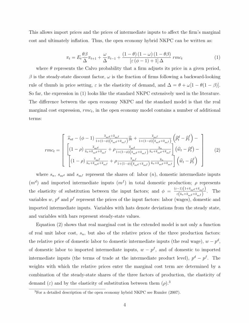
This allows import prices and the prices of intermediate inputs to affect the firm’s marginal
cost and ultimately inflation. Thus, the open economy hybrid NKPC can be written as:
πt = Etθβ
∆πt+1 +
ω
∆πt−1 +
(1 − θ) (1 − ω) (1 − θβ)
[ε (φ − 1) + 1] ∆rmct (1)
where θ represents the Calvo probability that a firm adjusts its price in a given period,
β is the steady-state discount factor, ω is the fraction of firms following a backward-looking
rule of thumb in price setting, ε is the elasticity of demand, and ∆ = θ + ω[1 − θ(1 − β)].
So far, the expression in (1) looks like the standard NKPC extensively used in the literature.
The difference between the open economy NKPC and the standard model is that the real
marginal cost expression, rmct, in the open economy model contains a number of additional
terms:
rmct =
snt − (φ − 1)
smd+s
mf
1+(1−φ)(smd+s
mf )yt +
smf
1+(1−φ)(smd+s
mf )
(pd
t − pft
)−[
(1 − ρ)smd
sn+smd+s
mf+ ρ
smd
1+(1−φ)(smd+s
mf )sn
sn+smd+s
mf
] (wt − pd
t
)−[(1 − ρ)
smf
sn+smd+s
mf+ ρ
smf
1+(1−φ)(smd+s
mf )sn
sn+smd+s
mf
] (wt − pf
t
) (2)
where sn, smd and smf represent the shares of: labor (n), domestic intermediate inputs
(md) and imported intermediate inputs (mf ) in total domestic production; ρ represents
the elasticity of substitution between the input factors; and φ =(ε−1)(1+s
md+smf )
ε(sn+smd+s
mf ). The
variables w, pd and pf represent the prices of the input factors: labor (wages), domestic and
imported intermediate inputs. Variables with hats denote deviations from the steady state,
and variables with bars represent steady-state values.
Equation (2) shows that real marginal cost in the extended model is not only a function
of real unit labor cost, sn, but also of the relative prices of the three production factors:
the relative price of domestic labor to domestic intermediate inputs (the real wage), w − pd,
of domestic labor to imported intermediate inputs, w − pf , and of domestic to imported
intermediate inputs (the terms of trade at the intermediate product level), pd − pf . The
weights with which the relative prices enter the marginal cost term are determined by a
combination of the steady-state shares of the three factors of production, the elasticity of
demand (ε) and by the elasticity of substitution between them (ρ).3
3For a detailed description of the open economy hybrid NKPC see Rumler (2007).
4

2.2 Forecasting from the NKPC
The method we propose for generating multi-step forecasts from the NKPC uses the present-
value formulation of the NKPC rather than the original formulation in difference form. Using
the original formulation would only have allowed for a nowcasting exercise as inflation ex-
pectations formed at future periods (and that would have been needed for forecasting at the
t + 1 period or further out) are not available by definition.
Our approach uses the concept of the fundamental rate of inflation as introduced by Galı
and Gertler (1999) as a starting point and extends this concept by generating a forecast of
fundamental inflation which we interpret as the inflation forecast implied by the NKPC. The
idea of fundamental inflation ultimately goes back to Campbell and Shiller (1987) but had
until recently been mainly used to assess the empirical fit of the NKPC by comparing it to
actual inflation. Using fundamental inflation for forecasting was first considered in Rumler
and Valderrama (2009) where a more thorough discussion of the method can be found.
To demonstrate how we further add to the above idea, we find it convenient to start from
the reduced-form hybrid NKPC
πt = γfEt (πt+1) + γbπt−1 + λ rmct (3)
To arrive at fundamental inflation, the NKPC is solved forward for current inflation. The
solution yields inflation as a function of the discounted sum of present and future marginal
costs. In the case of the hybrid NKPC the present-value representation is given by:
πt = δ1πt−1 +
(λ
δ2γf
) ∞∑s=0
(1
δ2
)s
Et[rmct+s] (4)
where δ1 =1−√
1−4γf γb
2γfand δ2 =
1+√
1−4γf γb
2γfare the stable and unstable roots of the hybrid
NKPC with the reduced-from coefficients being calculated from the estimated structural
parameters. Computing fundamental inflation according to equation (4) requires multi-period
forecasts of marginal cost. Campbell and Shiller (1987) propose to generate them from
a separately-estimated unrestricted bivariate VAR defined for inflation and real marginal
costs. Constrained by limited sample sizes, for our part we assume a univariate autoregressive
process to represent the evolution of real marginal cost.4
4In examining model fit, Kurmann (2005) stresses the importance of the chosen marginal cost specification
5

So far, in applications making use of the concept of fundamental inflation, the NKPC
and the equation that is used to forecast marginal cost (the auxiliary model) are estimated
at separate stages. This two-step approach implies a loss in efficiency and in statistical
precision since separately-estimated coefficients are only combined at the last stage (to derive
the forecast). An innovation in this paper is that we estimate the NKPC and the process for
marginal costs concurrently, at the estimation stage. To demonstrate this, we can write the
hybrid NKPC and the auxiliary model in state-space form:πt
Zt
=
γf~0 ′
~0 0
Et
πt+1
Zt+1
+
γb λ~a1
~0 A
πt−1
Zt−1
(5)
where Z is a vector of dimension p corresponding to an AR(p) process containing up
to p − 1 lags of real marginal cost, i.e. Zt =[rmct rmct−1 · · · rmct−p+1
]′, ~0 and 0 are
a vector and matrix of dimension p containing zeros and A is the companion matrix of a
V AR(1) for Z with ~a1 being its first row.
The solution of this system of second-order difference equations in (5) can be expressed
as the following first-order difference equation system:πt
Zt
=
δ1λ
δ2γf
~b1
~0 A
πt−1
Zt−1
(6)
where ~b1 is the first row of the matrix B = A[I − 1
δ2A
]−1
. Note that the first equation of
(6) is the empirical evaluation of (4) where the matrix summation formula has been applied
in the AR-forecast of future marginal cost. This expression can be used to derive a one-step-
ahead forecast of fundamental inflation.
Finally, we can use this one-step-ahead forecast to iteratively construct multi-step-ahead
forecasts of πt. For an h-steps-ahead forecast the generalized system is given as:
πt+h
Zt+h
=
δh1
h−1∑i=0
δi1
λδ2γf
~b1(h)
~0 Ah
πt
Zt
(7)
where ~b1(h) is the first row of B(h) = Ah[I − 1
δ2A
]−1
. From this expression we de-
for fundamental inflation. Although we focus in this paper on forecasting performance and not on in-samplefit, we nonetheless experimented with alternative lags for the autoregressive process.
6

rive 1-step, 4-step and 8-step-ahead NKPC-based semi-structural forecasts of inflation. For
later reference, we designate the above semi-structural model (SSM) with the open-economy
definition of marginal cost as SSM-OE, and its closed-economy version as SSM-CE.
3. Identification Issues and Estimation
There is by now ample evidence that when taken to the data NKPC equations, and indeed
DSGE models in general, face pervasive identification problems.5 The difficulties arise essen-
tially because of the presence of endogeneity, parameter non-linearity and weakly-informative
instruments or driving processes, combinations of which can lead to weak identification. The
latter causes the breakdown of standard asymptotic estimation and test procedures (such as
t-tests, J-tests, and Wald-type confidence intervals) making inference unreliable.6 More im-
portantly, standard estimation and test methods cannot alert the researcher to the presence
of the weak identification problem leaving it to go unnoticed.
To understand the above intuitively, consider the case of a model parameter that is
unidentifiable from the available data. In this case, a valid econometric method should be
able to indicate that all admissible values within the parameter’s space are equally acceptable
and should be found in the estimate’s confidence set. In other words, non-identification should
in principle lead to possibly-unbounded confidence sets that can alert the researcher to the
problem. Yet, typically-relied-on Wald-type confidence intervals are bounded by construction
and therefore inappropriate in the context of weak identification.7
Since identifying restrictions typically imply nonlinearity and discontinuous parameter
spaces, weak identification is almost inherent to the definition of structural models. As ex-
plained above, usual point and interval estimation methods, whether based on maximum
likelihood, on matching moments, or instrumental variable methods, and whether one con-
siders a single structural equation or a multi-equation structural system, are thus poten-
5For a few examples see Canova and Sala (2009), Dufour, Khalaf, and Kichian (2006), Stock and Wright(1997).
6For details see Dufour (1997), Dufour (2003), Staiger and Stock (1997), Wang and Zivot (1998), Zivot,Startz, and Nelson (1998), Dufour and Jasiak (2001), Kleibergen (2002), Kleibergen (2005), Stock, Wright,and Yogo (2002), Moreira (2003), Dufour and Taamouti (2005b), Dufour and Taamouti (2007), and Andrews,Moreira, and Stock (2006).
7These problems should not be confused with having very large estimated standard errors or poorly-approximated cut-off points.
7

tially flawed and should be avoided. Inference problems are averted if one applies instead a
confidence-set-based method that allows for unbounded outcomes. Such methods are known
as identification-robust methods.
3.1 Identification-Robust Method and Application
Identification-robust methods make use of inference procedures where error probabilities can
be controlled in the presence of endogeneity, nonlinear parameter constraints and identifica-
tion difficulties. Our approach follows the general theory developed in Dufour and Taamouti
(2005a), Dufour and Taamouti (2005b), and Dufour and Taamouti (2007). We propose confi-
dence set (CS) parameter estimates based on “inverting” identification-robust test statistics,
where inverting a test produces the set of parameter values that are not rejected by this
test. The least-rejected parameter vector in this set is the so-called Hodges-Lehmann point
estimates (see Hodges and Lehmann 1963, 1983, Dufour, Khalaf, and Kichian 2006, Du-
four, Khalaf, and Kichian 2009a, Dufour, Khalaf, and Kichian 2009b). In contrast to the
usual t-type confidence intervals, confidence sets formed by inverting a test can lead to un-
bounded solutions—a prerequisite for ensuring reliable coverage (see Dufour 1997). Thus,
extremely-wide confidence sets reveal important identification difficulties. In addition, if all
economically-relevant values of a model’s deep parameters are rejected at some chosen sig-
nificance level, the confidence set will be empty and we can infer that the model is rejected.
This provides an identification-robust alternative to the standard GMM-based J-test.
Both Galı, Gertler, and Lopez-Salido (2005) and Fernandez-Villaverde, Rubio-Ramirez,
and Sargent (2005) emphasize the fact that, whether inference is based on a single structural
equation, on the closed form, or on a structural system, the econometric method should
formally take into account the constraints on the parameters and/or error terms implied
by the underlying theoretical structure. In this respect, the tests that we invert not only
ensure identification-robustness, but they also maintain the structural aspect of the model
by permitting the formal imposition of the restrictions that map the theoretical model into
the econometric one. This is done respecting the calibration exercise and the structure of
the error term.
8

3.2 Application
Applications of identification-robust methods to the NKPC and to DSGE models have pre-
viously been made, for example, in Dufour, Khalaf, and Kichian 2006, Dufour, Khalaf, and
Kichian 2009a and Dufour, Khalaf, and Kichian 2009b.
Consider again the model in equation (1). Under rational expectations Etπt+1 = πt+1+vt.
We substitute the expectation term in the equation by its expression. In addition, we assume
a second-order autoregressive function for the exogenous process for rmct8. Combining these
two equations, we obtain the following estimation model:
πt =θβ
∆πt+1 +
ω
∆πt−1 +
(1 − θ) (1 − ω) (1 − θβ)
[ε (φ − 1) + 1] ∆(c + ψ1rmct−1 + ψ2rmct−2) + ut , (8)
where ∆ and rmct are defined according to their expressions in Section 2.
The resulting model is a special case of the general model presented in equations (6)-(7)
of Section 2. We first calibrate some of the parameters of the model. As is standard in
the literature, the discount rate β is set to 0.99 and the elasticity of demand ε is set to 11,
implying a markup of 10 per cent. The latter, along with the sample means for sn, sm, and
sf determine the calibrated value of φ (which is also present in the definition of real marginal
costs).
For a given subsample, the parameters of the autoregressive process are estimated by
ordinary least squares and the estimates are plugged into the above expression in equation
(8). Collecting these along with the calibrated parameters in a vector, we have
τ =(
β ε φ c ψ1 ψ2
)′.
To obtain a confidence set with level 1−α for the deep parameters θ and ω, we invert an
identification-robust test (see below) associated with the null hypothesis
H0 : θ = θ0, ω = ω0, and τ = τ0, (9)
where ω0 and θ0 are known values. Formally, this implies collecting the joint values of θ0 and
ω0 that given τ0 are not rejected by the test at level α.
8We also experimented with alternative lag lenghts for this autoregressive process obtaining qualitativelysimilar results.
9

The test is conducted in the context of the Anderson-Rubin regression given by π∗t =
ΓZt + ut where Zt is a vector of instruments (we use lags of inflation, cubically-detrended
output gap, change in nominal wages, and change in commodity prices) and
π∗t =
θ0β0
∆0
πt+1 +ω0
∆0
πt−1 +(1 − θ0) (1 − ω0) (1 − θ0β0)
[ε0 (φ0 − 1) − 1] ∆0
(c0 + ψ1,0rmct−1 + ψ2,0rmct−2) (10)
In the context of this transformed regression, the idea is then to test the joint significance
of the coefficients on the instruments.9 A grid-search method is used to sweep all of the
relevant choices for ω and θ. In each case we compute test statistics and their associated p-
values. The parameter vectors for which the p-values are greater than level α thus constitute
an identification-robust confidence set with level 1 − α. Following the Hodges-Lehmann
strategy (see Hodges and Lehmann (1963) and Hodges and Lehmann (1983)), a point estimate
can be obtained within this set by picking out the parameter value combination that is
associated with the highest p-value, or in other words, that is least-rejected.
4. Competing models
In this part we briefly describe the time series models and the backward-looking structural
model used in the comparison of the different forecasting models. As mentioned before, time
series models have been shown to perform relatively better in the short and medium run in
forecasting than structural models while the latter appear to have more merits in the long
run.
Among time series models, the AR and VAR specifications are the most straightforward
and, given their good performance, have been the most widely used models for inflation
forecasting.10 Specifically, we use AR(1) and AR(4) models as our univariate alternative to
the structural and semi-structural models. An AR(4) is used because we work with quarterly
data which might be correlated up to the fourth lag. The AR(1) is presented as well because
it proved to be the best performing of the AR specifications up to lag 4 and therefore is also
used as the benchmark against which all other models are evaluated, i.e. we express all root
mean square errors relative to the AR(1) forecast.
9For details of the test please refer to the references cited in this section.10We focus here on simple forecasting models. Other specifications such as static or dynamic factor models
could also be considered as they were shown to have good forecasting properties in the past.
10

A bivariate VAR model including inflation and real marginal cost is a very interesting
comparison model in our setup because it is actually the unrestricted and thereby encom-
passing version of our structural and semi-structural models. Comparing the forecasting
performance of the VAR and these models can thus be seen as a test of the restrictions
imposed by the particular structure of the NKPC and the semi-structural model improves
upon the performance of the unrestricted model. We choose the lag length of the VAR to be
2 in accordance with the AR(2) process assumed for real marginal cost in the semi-structural
model.
The random walk forecast is a very common benchmark for forecast comparisons and also
proves to be difficult to beat in cases where the variable to be forecast is characterized by a
high degree of persistence.
We also include the model proposed by Atkeson and Ohanian (2001) in our comparison
because they have shown that for the U.S. case no model they considered could improve upon
a four-quarter random walk model. Stock and Watson (2008) call this forecast “a milestone
in the forecasting literature” and use it as their benchmark model. As Atkeson and Ohanian
(2001) consider year-on-year inflation, we have to adapt their idea to our quarterly setup.
Their original model would specify that yearly inflation in 4 quarters is equal to yearly
inflation now. We adapt this idea by saying that quarterly inflation in 4 quarters is equal
to the average quarterly inflation over the last 4 historical quarters. Even though Atkeson
and Ohanian (2001) had proposed their model only for the 4-quarter-ahead horizon case,
for completeness, we apply their idea also to the 1-quarter and the 8-quarters-ahead horizon
cases. In this sense, our forecasts are more precisely “inspired by Atkeson and Ohanian
(2001)”.
Finally, to assess whether the specific structure of the NKPC, i.e. its forward-looking com-
ponent and the real marginal cost term, is important for its forecasting performance, we also
derive a forecast from a traditional Phillips Curve (PC) equation which includes backward-
looking inflation, the output gap and a supply shock variable. After some experimentation
with different supply shock variables, we estimate the following model:
πt = α0 + α1πt−1 + α2yt−h + α3∆rcpt−h + εt (11)
where h = 1, 4, 8 depending on the forecast horizon and yt is the output gap calculated
11

the same way as the one entering real marginal cost in (2), ∆rcpt is the quarterly change in
real commodity prices and εt are i.i.d. residuals.
5. Forecast Evaluation
As we are interested in the forecasting performance of the different models in the short as
well as the medium run we construct series of 1-quarter, 4-quarters and 8-quarters-ahead
pseudo out-of-sample forecasts from each model. The forecasts are generated in a recursive
exercise with a moving estimation window of 16 years starting in 1984. Specifically, we start
estimating the models for the period 1984Q1 to 1999Q4, generate 1-period, 4-periods and 8-
periods-ahead forecasts, move one quarter forward and calculate new 1-period, 4-periods and
8-periods-ahead forecasts, and so on.11 By stacking the last forecast values of each forecast we
obtain series of 1-step, 4-step and 8-step-ahead forecasts which are used to compute forecast
error and test statistics.
Our forecast evaluation period goes from 2000Q1 to 2008Q4 which gives us a total of 36
observations to compare. We have to note, though, that the small sample size is probably an
issue in our case for both, the estimation and the evaluation of the models. Either period,
however, could only be extended at the expense of the other.
5.1 Comparison of Root Mean Square Errors
We first assess the forecasting performance of the SSM and NKPC models, the AR, VAR,
the random walk (RW), Atkeson-Ohanian (AO) and the backward-looking Phillips Curve
(PC) models by calculating the root mean square errors (RMSE) for the different forecast
horizons. The results shown in Table 1 are expressed as RMSE ratios in relation to an AR(1).
We are using the AR(1) forecast as the benchmark because it proved to be the best among
the time-series models.12
11By this procedure we can claim that we at least partially account for structural changes that might haveoccurred at the beginning of our sample and which over time move out of the considered sample period.
12As a robustness check we also computed and compared RMSE’s leaving out two data points that corre-spond to one-time changes in Canadian taxes and might be driving some of the results. We find that RMSE’sare now smaller in all cases and that the AR(1) and VAR(2) models outperform the traditional NKPC atthe 1-step-ahead horizon. However, we also find that the SSM models continue to outperform all the others,with the open-economy version doing best at the 1-step and 8-step-ahead forecasts, and the closed-economyversion winning out at the 4-step-ahead horizon.
12

Table 1: Root Mean Square Forecasting Error (RMSE) for inflation forecasts based on the
different models by forecast horizon (calculated over the period 2000Q1-2008Q4)
RMSE 1-step RMSE 4-steps RMSE 8-steps
SSM − OE 0.913 0.940 0.974
SSM − CE 0.932 0.939 0.988
NKPC − OE 0.967 0.947 0.992
NKPC − CE 1.042 0.967 0.990
AR(1) 1 1 1
AR(4) 1.024 1.037 1.006
V AR(2) 1.001 1.006 1.039
RW 1.228 1.434 1.464
AO 1.034 0.998 1.079
PC 1.153 1.082 1.140
We can infer three general results from the table. First, the semi-structural and the NKPC
models appear to be quite successful in forecasting Canadian inflation at all horizons. With
only one exception – the closed-economy NKPC for the 1-step-ahead horizon – all structural
and semi-structural models (except for the backward-looking PC model) forecast better than
the time-series models. The fact that these models also outperform the time series models
in the short run probably reflects the role of the imbedded time-series features.
Second, the semi-structural models improve upon their structural alternatives in all cases.
Hence, the inclusion of the time-series component in the structural model seems to result in
a better predictive performance, although the differences in RMSE for the 4-step and the
8-step-ahead horizons are small.
Finally, open-economy model versions generally outperform their closed-economy coun-
terparts. In particular, for the 1-step and 8-step-ahead horizons, the open-economy specifi-
cation of the SSM model slightly outperforms the closed-economy specification, and for the
1-step and 4-step-ahead horizons, the open-economy NKPC outperforms its closed-economy
counterpart. Thus, not surprisingly, accounting for relative supply shocks is important in
forecasting Canadian inflation.
Another observation from Table 1 is that the semi-structural model outperforms the
more general VAR(2) at all horizons. We interpret this fact as evidence that the restrictions
13

imposed by the particular structure of the model enhances its predictive power.
Further, the random walk forecast, which was shown to be difficult to outperform es-
pecially in the short run in other countries, turns out to be an unsuccessful alternative for
Canadian CPI inflation at all horizons. The Atkeson and Ohanian (2001) model does a good
job in forecasting only at the 4-quarter horizon which is the horizon for which it was orig-
inally designed. Finally, the backward-looking PC model augmented with a supply shock
variable is not very successful in forecasting Canadian inflation at any horizon as it is able
to outperform only the RW forecast. This indicates that the forward-looking component of
the Phillips Curve does matter for its forecasting performance.
5.2 Significance Tests
While at first glance the overall performance of the semi-structural models is impressive versus
time-series models, some tests of the significance of the difference in forecasting performance
between the SSMs and the competing models is still called for. Below we report the results
from the Diebold-Mariano test of equality of expected loss as modified by Harvey, Leybourne,
and Newbold (1997), as well as a modified sign test of equality of squared error.
5.2.1 Modified Diebold-Mariano test
We define the loss differential at time t dt as
dt = g(e1,t) − g(e2,t) (12)
where g(x) is the loss from an error of size x, and ei,t is the forecast error at time t from
model i.
The Diebold-Mariano test is a test of the hypothesis H0 : µd = 0, where we define d as
the mean loss differential
d =1
P
P∑j=1
dt, (13)
where P is the number of forecasts. As P gets large,
(d − µd) →d N(0, Vd/P ), (14)
14

where
Vd ≡∞∑
τ=−∞E(dt − µd)(dt−τ − µd). (15)
We can, naturally, obtain a HAC kernel estimate of Vd by calculating
Vd =1
P
P−1∑τ=−(P−1)
P∑t=|τ |+1
L(τ
τmax
)(dt − d)(dt−τ − d), (16)
where L(x) is a lag window and τmax is the truncation lag. Diebold and Mariano (1995)
use a rectangular lag window such that L(x) = 1 for x ≤ 1 and zero otherwise, and set
τmax = h − 1 where h is the number of periods ahead of the forecast, but other lag window
functions are also possible. In our application, we use a Bartlett kernel such that L(x) = 1−x
for x ≤ 1 and zero otherwise, picking the optimal τmax using the automatic bandwidth
selection technique of Andrews (1991). We find that for most comparisons the optimal lag
length is well above the upper bound suggested by Diebold and Mariano’s rectangular kernel.
While the Diebold-Mariano t-statistic
tDM =d√Vd
×√
P (17)
converges to a N(0, 1) distribution asymptotically, Vd will be biased downward in small
samples, as Harvey, Leybourne, and Newbold (1997) have pointed out. They suggest the
following modified t-statistic:
tMDM = tDM ×√
P + 1 − 2h + (h−1)hP
P=
d√Vd
×√
P + 1 − 2h +(h − 1)h
P(18)
and comparing it to a t-distribution with P − 1 degrees of freedom. For cases such as our
eight-step ahead forecasts (P = 29, h = 8) the effect of the correction can be substantial.13
Whether a forecasting model is “significantly” better than another also depends in part
on the loss function. The most common loss function is one proportional to squared error,
of course, but others are possible. Here, we look at:
13This, admittedly, is not the only possible source of bias; in particular, some of the models are nested inthe others (which will tend to favour the smaller model in small samples), and P is large compared to thedata set used in estimation, introducing extra uncertainty from variation in model parameters. Both sourcesof bias could be substantial.
15

• a loss function proportional to squared forecast error (g(x) = x2), so that dt = e21,t−e2
2,t;
and
• a loss function proportional to the absolute value of forecast error (g(x) = |x|, so that
dt = |e1,t| − |e2,t|.
5.2.2 Modified sign test
We also look at a modified version of a simple sign test, letting dt equal -1 if e21,t < e2
2,t and
1 otherwise, and testing the hypothesis H0 : µd = 0, as above. If the loss differentials are iid
with mean zero (as they should be for one-step-ahead forecast errors), the distribution of d
should converge to N(0, P ) as P gets large. If there is evidence that the loss differentials are
serially correlated (and they generally are for four and eight step ahead forecasts), a kernel
estimate of the variance of dt is used instead and the resulting t-statistic corrected as with
the modified Diebold-Mariano statistic.
5.3 Results and discussion
Table 2 lists the t-statistics from the comparisons of each pair of models at the one-step
horizon. One step ahead, and based on a squared-error criterion, our semi-structural open-
economy model is clearly the best available, significantly beating all the atheoretical time-
series models and the backward-looking PC model. In the medium term, (i.e., four steps
ahead–Table 3), the semi-structural open-economy model is overall still the best; in each of
the tests reported, this model beats the AR, VAR and PC specifications, but its performance
is not significantly better than that of the Atkeson-Ohanian forecast.
Finally, eight steps ahead (Table 4), the semi-structural open-economy model remains the
best of the structural models, but its performance is no longer significantly better than any
of the time series models (except for the naive no-change forecast) as well as the PC model.14
A few broad generalizations can be made. Semi-structural models using information from
our measures of marginal cost are, in general, more useful in forecasting inflation in the short
and medium run than are time series models (with the possible exception of an Atkeson-
Ohanian forecast). We also note some forecasting improvement when using semi-structural
over conventional NKPCs, though the gain is smaller and not always robust to the adopted
14Results should be interpreted with caution in this case as sample sizes are quite small.
16

test definition. The same is true regarding improvement in forecasts from using an open-
over a closed-economy marginal cost measure.
6. Conclusion
We proposed semi-structural single-equation models to forecast inflation in Canada in the
short and medium terms. The models combine structural features from the NKPC, including
open and closed-economy alternatives, with time-series features present in the data. Given
that NKPC models are typically plagued with identification problems, we used identification-
robust methods to estimate key structural parameters.
We found that our semi-structural NKPC models improve upon the short and medium-
run forecasting performance over alternative models. The latter include conventional time
series models such as unrestricted bivariate VARs, as well as traditional NKPC models and
a backward-looking Phillips Curve model, though statistical significance could only be es-
tablished against the former category of models and the PC model. In addition, we found
open-economy model versions to generally have better forecasting performance (though not
significantly so) than their closed-economy counterparts, which is not surprising given that
Canada is an open economy and that relative price shocks are known to matter.
One caveat of the present study is the limited sample sizes that are available to us. With
more observations in future, statistical methods should better help us discriminate between
the competing alternatives.
17

References
Andrews, D.W.K. 1991. “Heteroskedasticity and Autocorrelation Consistent Covariance Ma-
trix Estimation.” Econometrica 59: 817–858.
Andrews, D.W.K., M.J. Moreira, and J.H. Stock. 2006. “Optimal Two-Sided Invariant Sim-
ilar Tests for Instrumental Variables Regression.” Econometrica 74: 715–752.
Atkeson, A. and L. Ohanian. 2001. “Are Phillips Curves Useful for Forecasting Inflation?”
Federal Reserve Bank of Minneapolis Quarterly Review 25(1): 2–11.
Bernanke, B., J. Boivin, and P. Eliasz. 2005. “Measuring the Effects of Monetary Policy:
A Factor-Augmented Vector Autoregressive (FAVAR) Approach.” Quarterly Journal of
Economics 120: 387–422.
Campbell, J.Y. and R.J. Shiller. 1987. “Cointegration and Tests of Present Value Models.”
Journal of Political Economy 95: 1062–1088.
Canova, F. and L. Sala. 2009. Back to Square One: Identification Issues in DSGE Models.
Technical report, Centre for Economic POlicy Research Discussion Paper 7234, London,
England.
Cogley, T. and A. Sbordone. 2008. “Trend Inflation, Indexation, and Inflation Persistence in
the New Keynesian Phillips Curve.” American Economic Review 98: 2101–26.
Del Negro, M. and F. Schorfheide. 2006. “How good is what you’ve got? DSGE-VAR as a
toolkit for evaluating DSGE models.” Economic Review, Federal Reserve Bank of Atlanta
2: 21–37.
Del Negro, M., F. Schorfheide, F. Smets, and R. Wouters. 2007. “On the Fit of New Keynesian
Models.” Journal of Business and Economic Statistics 25: 123–43.
Diebold, F.X. and R.S. Mariano. 1995. “Comparing Predictive Accuracy.” Journal of Busi-
ness and Economic Statistics 13: 253–263.
Dufour, J.M. 1997. “Some Impossibility Theorems in Econometrics, with Applications to
Structural and Dynamic Models.” Econometrica 65: 1365–89.
18

———. 2003. “Identification, Weak Instruments and Statistical Inference in Econometrics.”
Canadian Journal of Economics 36(4): 767–808.
Dufour, J.M. and J. Jasiak. 2001. “Finite Sample Limited Information Inference Methods
for Structural Equations and Models with Generated Regressors.” International Economic
Review 42: 815–43.
Dufour, J.M., L. Khalaf, and M. Kichian. 2006. “Inflation dynamics and the New Keyne-
sian Phillips Curve: an identification robust econometric analysis.” Journal of Economic
Dynamics and Control 30: 1707–1728.
———. 2009a. “Assessing Indexation-based Calvo Inflation Models.” Working Paper 2009-7,
Bank of Canada.
———. 2009b. “Structural Multi-Equation Macroeconomic Models: Identification-Robust
Estimation and Fit.” Working Paper 2009-19, Bank of Canada.
Dufour, J.M. and M. Taamouti. 2005a. Point-Optimal Instruments and Generalized
Anderson-Rubin Procedures for Nonlinear Models. Technical report, C.R.D.E., Univer-
site de Montreal.
———. 2005b. “Projection-Based Statistical Inference in Linear Structural Models with
Possibly Weak Instruments.” Econometrica 73: 1351–1365.
———. 2007. “Further Results on Projection-Based Inference in IV Regressions with Weak,
Collinear or Missing Instruments.” Journal of Econometrics 139: 133–153.
Fernandez-Villaverde, J., J. Rubio-Ramirez, and S. Sargent. 2005. A,B,C’s (And D’s) For
Understanding VARS. Technical report, University of Pennsylvania.
Galı, J. and M. Gertler. 1999. “Inflation Dynamics: A Structural Econometric Analysis.”
Journal of Monetary Economics 44: 195–222.
Galı, J., M. Gertler, and J.D. Lopez-Salido. 2005. “Robustness of the Estimates of the Hybrid
New Keynesian Phillips Curve.” Journal of Monetary Economics 52: 1107–18.
Harvey, D., S. Leybourne, and P. Newbold. 1997. “Testing the Equality of Prediction Mean
Squared Errors.” International Journal of Forecasting 13: 281–291.
19

Hodges, J.L., Jr. and E.L. Lehmann. 1963. “Estimates of Location Based on Rank Tests.”
Annals of Mathematical Statistics 34: 598–611.
———. 1983. “Hodges-Lehmann Estimators.” In Encyclopedia of Statistical Sciences, Volume
3, edited by N.L. Johnson, S. Kotz, and C. Read, 642–45. New York: John Wiley & Sons.
Kleibergen, F. 2002. “Pivotal Statistics for Testing Structural Parameters in Instrumental
Variables Regression.” Econometrica 70(5): 1781–1803.
———. 2005. “Testing Parameters in GMM Without Assuming that They Are Identified.”
Econometrica 73: 1103–1123.
Kurmann, A. 2005. “Quantifying the Uncertainty about the Fit of a New Keynesian Pricing
Model.” Journal of Monetary Economics 56(6): 1119–1134.
Mavroeidis, S. 2005. “Identification issues in forward-looking models estimated by GMM
with an application ot the Phillips curve.” Journal of Money, Credit and Banking 37:
421–449.
Moreira, M.J. 2003. “A Conditional Likelihood Ratio Test for Structural Models.” Econo-
metrica 71(4): 1027–48.
Nason, J. and G. Smith. 2008. “Identifying the New Keynesian Phillips Curve.” Journal of
Applied Econometrics 23: 525–51.
Rumler, F. 2007. “Estimates of the Open Economy New Keynesian Phillips Curve for Euro
Area Countries.” Open Economies Review 18(4): 427–51.
Rumler, F. and M.T. Valderrama. 2009. “Comparing the New Keynesian Phillips Curve
with Time Series Models to Forecast Inflation.” North American Journal of Economics
and Finance forthcoming.
Sbordone, A. 2007. “Inflation Persistence: Alternative Interpretations and Policy Implica-
tions.” Journal of Monetary Economics 54: 1311–39.
Smets, F. and R. Wouters. 2003. “An Estimated Stochastic General Equilibrium Model of
the Euro Area.” Journal of the European Economic Association 1: 1123–75.
20

———. 2007. “Shocks and Frictions in US Business Cycles: A Bayesian DSGE Approach.”
American Economic Review 97(3): 587–606.
Staiger, D. and J.H. Stock. 1997. “Instrumental Variables Regression with Weak Instru-
ments.” Econometrica 65(3): 557–86.
Stock, J.H. and M.W. Watson. 2008. Phillips Curve Inflation Forecasts. Discussion paper,
NBER Working Paper No. 14322.
Stock, J.H. and J.H. Wright. 1997. GMM with Weak Identification. Technical report, Kennedy
School of Government, Harvard University. Forthcoming in Econometrica.
Stock, J.H., J.H. Wright, and M. Yogo. 2002. “A Survey of Weak Instruments and Weak
Identification in Generalized Method of Moments.” Journal of Business and Economic
Statistics 20(4): 518–29.
Wang, J. and E. Zivot. 1998. “Inference on Structural Parameters in Instrumental Variables
Regression with Weak Instruments.” Econometrica 66(6): 1389–1404.
Zivot, E., R. Startz, and C.R. Nelson. 1998. “Valid Confidence Intervals and Inference in the
Presence of Weak Instruments.” International Economic Review 39: 1119–44.
21

Appendix: Data
The quarter-on-quarter log change of the Canadian CPI (seasonally adjusted) is used as
the dependent variable in all estimations. For the estimation of the semi-structural models
and the NKPC real unit labor cost, sn, is defined as the total compensation to employees
divided by nominal GDP, and smd as well as smf are the ratios of domestically produced and
imported intermediate goods to nominal GDP. Compensation per employee is used for w and
the Canadian producer price subindex for intermediate goods and the import deflator are
used as proxies for and pd and pf , respectively. Input/Output tables available for the sample
period were used to separate intermediate inputs into domestic and imported shares.
We use cubically-detrended measures of the output gap and of real marginal cost which
are defined in a real-time sense, i.e. the gap value at time t does not use information beyond
that date. Specifically, as in Dufour, Khalaf, and Kichian (2006) for example, the trend is
first estimated with data ending in t and a gap value is calculated as the deviation of the
original series from the trend for time t. Then the sample is extended by one observation
and the trend is re-estimated which is used to calculate a value for the gap for time t + 1.
The process is repeated in this fashion until the end of the sample.
All variables in the recursive estimation procedure are calculated as deviations from their
means.
22

Figure 1: Inflation and Open-Economy Real Marginal Cost
-1.0
-0.5
0.0
0.5
1.0
1.5
2.0
2.5
3.0
-.04
-.03
-.02
-.01
.00
.01
.02
.03
.04
84 86 88 90 92 94 96 98 00 02 04 06 08
qoq CPI inflation (sa) rm c oe
Figure 2: Inflation and closed-Economy Real Marginal Cost
-1.0
-0.5
0.0
0.5
1.0
1.5
2.0
2.5
3.0
-.08
-.06
-.04
-.02
.00
.02
.04
.06
.08
84 86 88 90 92 94 96 98 00 02 04 06 08
qoq CPI inflation (sa) rm c ce
23

Appendix: Tables
Table 2: Tests of significant differences in forecasting performance, one step ahead
(a): Modified Diebold-Mariano, H0 : Ee2row − Ee2
column = 0SSM-CE NKPC-OE NKPC-CE AR(1) AR(4) VAR(2) RW AO PC
SSM-OE -0.49 -1.06 -1.21 -2.17** -2.50** -1.87* -2.22** -1.97* -2.39**SSM-CE -1.22 -1.40 -1.42 -1.72* -1.43 -2.01* -1.72* -1.95*NKPC-OE -1.18 -0.55 -0.91 -0.63 -1.79* -1.05 -1.61NKPC-CE 0.38 0.17 0.43 -1.17 0.08 -0.77AR(1) -1.11 -0.04 -2.15** -0.65 -2.34**AR(4) 0.78 -1.80* -0.27 -1.74*VAR(2) -1.97* -0.67 -2.00*RW 1.55 1.13AO -1.28
(b): Modified Diebold-Mariano, H0 : E|erow| − E|ecolumn| = 0SSM-CE NKPC-OE NKPC-CE AR(1) AR(4) VAR(2) RW AO PC
SSM-OE 0.22 -0.56 -1.19 -1.76* -2.16** -1.77* -1.81* -2.03** -3.45***SSM-CE -0.96 -1.60 -2.18** -2.45** -2.42** -2.02* -2.09** -3.52***NKPC-OE -1.00 -1.23 -1.44 -1.28 -1.61 -1.56 -2.67**NKPC-CE -0.17 -0.43 -0.11 -1.42 -0.77 -2.31**AR(1) -0.71 0.07 -1.54 -0.72 -3.69***AR(4) 0.39 -1.20 -0.63 -2.42**VAR(2) -1.47 -0.65 -2.92***RW 0.78 -0.49AO -1.42
(c): Modified sign test, H0 : med(e2row) − med(e2
column) = 0SSM-CE NKPC-OE NKPC-CE AR(1) AR(4) VAR(2) RW AO PC
SSM-OE 0.76 0 0 -1.04 -1.35 -1.40 -0.72 -1.35 -5.29***SSM-CE -1.43 -1.35 -2.09** -2.50** -3.45*** -1.55 -2.59** -7.32***NKPC-OE -0.38 -1.04 -1.43 -1.32 -1.27 -1.28 -5.29***NKPC-CE -2.50** -1.18 -1.71* -1.55 -1.81* -5.29***AR(1) 2.21** 0 -0.72 -1.11 -5.29***AR(4) 0 -1.50 -1.20 -4.57***VAR(2) -0.46 -0.42 -3.42***RW 1.04 -0.33AO -2.09**
Significance level: *=10 percent; **=5 percent; ***=1 percent.
24

Table 3: Tests of significant differences in forecasting performance, four steps ahead
(a): Modified Diebold-Mariano, H0 : Ee2row − Ee2
column = 0SSM-CE NKPC-OE NKPC-CE AR(1) AR(4) VAR(2) RW AO PC
SSM-OE 0.05 -0.31 -0.87 -2.57** -2.54** -1.77* -3.12*** -0.87 -1.75*SSM-CE -0.34 -1.39 -1.97* -2.18** -1.61 -2.94*** -0.85 -2.04**NKPC-OE -0.85 -1.99* -2.10** -2.28** -2.99*** -0.68 -1.87*NKPC-CE -1.39 -1.89* -0.94 -2.95*** -0.46 -1.86*AR(1) -1.79* -0.15 -2.85*** 0.03 -1.21AR(4) 0.59 -2.72** 0.72 -0.68VAR(2) -2.70** 0.09 -1.01RW 2.89*** 2.28**AO -0.83
(b): Modified Diebold-Mariano, H0 : E|erow| − E|ecolumn| = 0SSM-CE NKPC-OE NKPC-CE AR(1) AR(4) VAR(2) RW AO PC
SSM-OE 0.98 0.42 0.16 -1.58 -1.93* -1.38 -3.32*** -0.87 -0.95SSM-CE -0.49 -1.39 -2.46** -2.45** -1.88* -3.37*** -1.29 -1.99*NKPC-OE -0.22 -1.36 -1.44 -2.48** -3.28*** -1.06 -1.33NKPC-CE -2.16** -2.07** -1.29 -3.27*** -0.99 -1.76*AR(1) -1.77* -0.36 -3.10*** -0.28 -0.24AR(4) 0.30 -3.08*** 0.61 0.56VAR(2) -2.69** 0.07 0.15RW 3.42*** -2.78***AO 0.06
(c): Modified sign test, H0 : med(e2row) − med(e2
column) = 0SSM-CE NKPC-OE NKPC-CE AR(1) AR(4) VAR(2) RW AO PC
SSM-OE 1.11 -0.36 1.66 -3.68*** -2.64** -1.87* -3.34*** 0.47 -1.46SSM-CE -1.11 0.16 -3.68*** -3.34*** -1.81* -2.88*** 0.16 -2.22**NKPC-OE 0.39 -2.81*** -2.64** -1.81* -3.68*** -0.39 -1.46NKPC-CE -3.09*** -2.64** -0.94 -2.88*** 0.74 -1.82*AR(1) -1.56 -0.68 -3.18*** 1.11 -0.79AR(4) -0.15 -4.58*** 1.06 0.79VAR(2) -3.34*** 0.16 0.79RW 3.22*** -2.20**AO 0.47
Significance level: *=10 percent; **=5 percent; ***=1 percent.
25

Table 4: Tests of significant differences in forecasting performance, eight steps ahead
(a): Modified Diebold-Mariano, H0 : Ee2row − Ee2
column = 0SSM-CE NKPC-OE NKPC-CE AR(1) AR(4) VAR(2) RW AO PC
SSM-OE -0.67 -0.85 -0.67 -1.33 -1.19 -1.28 -2.53** -1.48 -1.11SSM-CE -0.15 -0.08 -0.47 -0.55 -0.88 -2.45** -1.20 -1.08NKPC-OE -0.07 -0.31 -0.54 -1.11 -3.52*** -1.41 -1.02NKPC-CE -0.44 -0.47 -0.76 -2.39** -1.10 -1.11AR(1) -0.39 -0.82 -2.48** -1.17 -1.06AR(4) -0.78 -1.57 -1.28 -0.99VAR(2) -2.44** -0.66 -0.78RW 2.60** 1.67AO -0.41
(b): Modified Diebold-Mariano, H0 : E|erow| − E|ecolumn| = 0SSM-CE NKPC-OE NKPC-CE AR(1) AR(4) VAR(2) RW AO PC
SSM-OE 0.12 -0.43 0.66 -1.17 -0.50 -1.64 -2.59** -1.92* -1.05SSM-CE -0.75 0.41 -0.80 -0.39 -1.61 -2.64** -1.88* -1.13NKPC-OE 0.72 -0.32 -0.04 -1.47 -2.55** -1.58 -0.90NKPC-CE -1.40 -0.86 -1.51 -2.65** -2.02* -1.23AR(1) 0.59 -1.30 -2.53** -1.71* -0.83AR(4) -1.22 -2.51** -1.77* -0.91VAR(2) -1.94* -0.17 0.05RW 2.23** 1.96*AO 0.16
(c): Modified sign test, H0 : med(e2row) − med(e2
column) = 0SSM-CE NKPC-OE NKPC-CE AR(1) AR(4) VAR(2) RW AO PC
SSM-OE 0.36 -0.11 1.30 -0.70 -0.70 -0.93 -1.64 -0.99 -2.89***SSM-CE -1.81* 0.11 -1.64 -0.70 -1.58 -3.13*** -1.44 -2.00*NKPC-OE 1.58 -0.99 -1.31 -0.93 -2.18** -1.66 -2.00*NKPC-CE -1.64 -0.70 -1.21 -2.18** -1.66 -2.00*AR(1) 1.31 -0.91 -1.48 -0.99 -1.30AR(4) -1.26 -2.00* -0.94 -0.99VAR(2) -0.99 -0.16 0.42RW 2.54 0.70AO 0.42
Significance level: *=10 percent; **=5 percent; ***=1 percent.
26