Semantics and Evaluation Techniques for Window Aggregates in Data Streams

Jin Li1, David Maier1, Kristin Tufte1, Vassilis Papadimos1, Peter A. Tucker2

1Portland State University 2Whitworth College Portland, OR, USA Spokane, WA, USA

{jinli, maier, tufte, vpapad}@cs.pdx.edu ptucker@whitworth.edu

ABSTRACT A windowed query operator breaks a data stream into possibly overlapping subsets of data and computes a result over each. Many stream systems can evaluate window aggregate queries. However, current stream systems suffer from a lack of an explicit definition of window semantics. As a result, their implementations unnecessarily confuse window definition with physical stream properties. This confusion complicates the stream system, and even worse, can hurt performance both in terms of memory usage and execution time. To address this problem, we propose a framework for defining window semantics, which can be used to express almost all types of windows of which we are aware, and which is easily extensible to other types of windows that may occur in the future. Based on this definition, we explore a one-pass query evaluation strategy, the Window-ID (WID) approach, for various types of window aggregate queries. WID significantly reduces both required memory space and execution time for a large class of window definitions. In addition, WID can leverage punctuations to gracefully handle disorder. Our experimental study shows that WID has better execution-time performance than existing window aggregate query evaluation options that retain and reprocess tuples, and has better latency-accuracy tradeoffs for disordered input streams compared to using a fixed delay for handling disorder.

1. INTRODUCTION Many types of data present themselves in stream format: environmental sensor readings, network monitoring data, telephone call records, traffic sensor data and auction bids, to name a few. For applications monitoring and processing streams, window aggregates are an important query feature. A window specifies a moving view that decomposes the stream into (possibly overlapping) subsets that we call window extents, and computes a result over each. (Think of a window specification as a “cookie cutter” and window extents as cookies cut with it.) For example, “compute the number of vehicles on I-95 between milepost 205 and milepost 245 over the past 10 minutes; update the count every 1 minute” is a window aggregate query where successive window extents overlap by 9 minutes.

Evaluating window aggregate queries over streams is non-trivial. The potential for high data-arrival rates, and huge data volumes, along with near real-time requirements in many stream applications, make memory and execution-time performance of stream query evaluation critical. Bursty and out-of-order data arrival raises problems with detecting the boundaries of window extents. Out-of-order arrival also complicates the process of determining the content of window extents and can lead to inaccurate aggregate results or high latency in the output of the results. We have observed that accommodating out-of-order arrival can introduce significant complexity into window query evaluation. We see two major issues with current stream systems that process window queries. One is the lack of explicit window semantics. As a result, the exact content of each window extent tends to be confused with window operator implementation and physical stream properties. The other issue is implementation efficiency, in particular, memory usage and execution time. To evaluate sliding-window aggregate queries where consecutive window extents overlap (i.e., each tuple belongs to multiple window extents), most current proposals keep all active input tuples in an in-memory buffer. In addition, each tuple is reprocessed multiple times—once for each window extent to which it belongs. We will propose an approach that avoids intra-operator buffering and tuple reprocessing.

In this paper, we present a framework for defining window semantics and a window query evaluation technique based on it. In the framework, we define window semantics explicitly—independent of any algorithm for evaluating window queries. From our definitions, it is clear that many commonly used types of windows do not depend on physical stream order. However, most existing window-query evaluation techniques assume that stream data are ordered or are ordered within some bound. Our window query evaluation technique, called the Window-ID (WID) approach, is suggested by the semantic framework. Our technique processes each input tuple on the fly as it arrives, without keeping tuples in buffers and without reprocessing tuples. Our experimental study shows significantly improved execution-time performance over existing evaluation techniques that buffer and reprocess tuples.

Permission to make digital or hard copies of all or part of this work for personal or classroom use is granted without fee provided that copies are not made or distributed for profit or commercial advantage and that copies bear this notice and the full citation on the first page. To copy otherwise, or republish, to post on servers or to redistribute to lists, requires prior specific permission and/or a fee.

In contrast to other techniques, WID can process out-of-order tuples as they arrive without sorting them into the “correct” order. It does not require a specific type of assumption about the physical order of data in the stream. Instead, it uses punctuation [16] to encode whatever kind of ordering information is available. In the later part of the paper, we examine real-life examples of

ACM SIGMOD 2005, June 14–16, 2005, Baltimore, Maryland, USA. Copyright 2005 ACM 1-59593-060-4/05/06…$5.00.

311

stream disorder and discuss disorder-handling methods. Slack [2] and heartbeats [14] are mechanisms proposed for handling disorder in input streams. Different means for handling disorder can affect the flexibility, scalability and performance of window-query evaluation approaches. We experimentally evaluated latency-accuracy tradeoffs in handling disorder using WID and sort-based slack.

SUSPECT

PRESUMPTIVE

CONFIRMED

INTERCEPTED

Figure 1: Four detection stations in a detection task (from Yonnel Gardes, The Transpo Group, Kirkland, WA, with permission)

This paper is organized as follows: Section 2 provides a running example that illustrates the basic concepts of WID; Section 3 introduces our framework for defining window semantics; Section 4 discusses implications of window semantics for query evaluation; Sections 5 and 6 present the implementation of WID; Section 7 analyzes disorder using network flow data and discusses mechanisms for handling it; Section 8 presents performance results; and Section 9 concludes.

2. RUNNING EXAMPLE We introduce a running example that illustrates the operations used in WID. Via this example, we show that with WID 1) there is no need to retain input tuples in buffers, although there may be queues to pass tuples between steps; 2) each tuple is processed only once at a given step; and 3) no assumptions about the physical order of the input are required. Consider a radiation-detection system that can be installed along freeways, such as the one under study in the New Jersey Turnpike Radiation Detection project at Lawrence Livermore National Lab [12]. A radiation-detection system identifies potentially dangerous vehicles, tracks them as they progress along the freeway, and targets a vehicle confirmed to have radioactive material for interception. Figure 1 shows four detection stations involved in a detection task on I-95 northbound from I-195 to the Holland Tunnel. While tracking vehicles, it is critical to accurately forecast travel time between detection stations, so that the system does not lose track of suspicious vehicles. One way to address this problem is to estimate the max and min travel time between stations. A freeway is separated into non-overlapping segments by adjacent ramps. Suppose that there exists a speed sensor (such as a pair of inductive loop detectors commonly found near freeway on-ramps) per segment along the freeway, and that speed readings are streamed to a central system, where the min and max speed for each segment of the freeway over the past five minutes are

computed, and updated periodically. Then, min and max travel time between stations can be calculated easily and continuously updated based on the current speed bound for each segment and the length of the segment. Assume the schema of speed sensor readings is <seg-id, speed, ts>, where seg-id is the segment id and ts is the timestamp for a sensor reading. We might choose to continuously compute the min and max speed of each segment by computing the min and max over the past 5 minutes, and updating the results every minute. We call this query Q1, shown below in a CQL-like language [3]. Note that the time notion (e.g., over the past 5 minutes) in Q1 is defined on the ts attribute of the sensor readings. Q1: SELECT seg-id, max(speed), min(speed) FROM Traffic [RANGE 300 seconds

SLIDE 60 seconds WATTR ts] GROUP BY seg-id

Figure 2 shows the steps that WID uses to process Q1. The details of the operators are given in later sections. The traffic-speed stream, with punctuations, arrives at the query system. Briefly, a punctuation is information embedded in a data stream indicating that no more tuples having certain attribute values will be seen in the stream. For example, punctuation p1 indicates that no more tuples will arrive from segment s6 that have a timestamp attribute value less than 12:11:00PM. In our example, we assume that each

(seg-id, speed, ts, wid) t1′ (s5, 47, 12:10:05, 10-14) t2′ (s6, 48, 12:10:02, 10-14) t3′ (s6, 50, 12:10:30, 10-14) p1′ (s6, *, *, 10 ) t4′ (s5, 47, 12:10:30, 10-14) p2′ (s5, *, *, 10 ) … …

tags with window-ids

group on seg-id and wid

wid seg-id max min

10 s5 47 47 10 s6 50 48 … … … … 14 s5 51 50 14 s6 52 50

(wid, seg-id, max, min) m1 (10, s6, 47, 47 ) m2 (10, s5, 50, 48 )

(seg-id, speed, ts) t1 (s5, 47, 12:10:05) t2 (s6, 48, 12:10:02) t3 (s6, 50, 12:10:30) p1 (s6, *, 12:11:00) t4 (s5, 47, 12:10:30) p2 (s5, *, 12:11:00) … …

Figure 2: Operations on input tuples, using the WID approach to evaluate Q1

312

individual sensor provides such a punctuation every minute. As Figure 2 shows, in the first step, each input tuple is tagged with a range of window-ids. In WID, each window extent is identified by a unique window-id. In this example, we use non-negative integers for window-ids. Suppose Q1 starts at 12:00:00PM. Each window extent is a 5-minute sub-stream, which overlaps with adjacent window extents. In our case, for example, window extent 10 is the 12:06:00PM – 12:11:00PM sub-stream; and window extent 11 is the 12:07:00PM – 12:12:00PM sub-stream. For each input tuple, we can calculate the window-ids for the window extents to which it belongs. For example, t1 belongs to window extents 10 through 14. A similar calculation is applied to punctuations. Input punctuations, which punctuate on the seg-id and ts attributes, are transformed into punctuations on the seg-id and wid attributes. For example, p1 is transformed into p1′, which indicates that no more tuples from the sensor at segment s6 for window extent 10 will arrive. Note that we extend the input scheme of the speed tuple by adding the wid as an explicit attribute. Also note that in the first step, each tuple or punctuation is processed immediately as it arrives, and is streamed out immediately after processing. The second step is an aggregation where tuples tagged with window-ids are grouped by the seg-id attribute, as well as the wid attribute. Note that a tuple tagged with a range of window-ids represents a set of tuples, each tagged with a single window-id. An internal hash table is used to maintain the partial max and min value for each group. Upon the arrival of a punctuation, the hash entry that matches the punctuation is output and purged from the hash table. For example, when punctuation p1′ arrives, m1 is output and its corresponding hash entry is cleared. Overall, introducing window-ids into query execution brings benefits to both performance and system implementation. It reduces operator buffer space and execution time; and it transforms window aggregate queries into group-by aggregate queries and thus reduces the implementation complexity of the system. Also observe that WID does not need to reorder tuples on ts, as long as punctuations are placed correctly. WID does require calculations for multiple window extents to be underway concurrently, but the storage overhead is trivial unless there are many more window extents than tuples.

3. WINDOW SEMANTICS As can be seen from our example, the key to WID is the association of tuples with window-ids. In this section we present a semantic framework that makes this association explicit, independent of any particular operator implementation. In Section 4 we return to window-aggregate evaluation based on this semantics.

3.1 Motivation In previous work, window semantics has often been described operationally. However, operational window definitions tend to lead to confusion of the window extent definition with physical data properties and implementation details. For example, some current window query operators process window extents sequentially— that is, they close the active window when a tuple past it arrives, which translates into a requirement that their input arrive in order of the windowing attribute. If the data is not in order, some sort mechanism such as Aurora’s BSort [2] must be

used to reorder the data. Without a mechanism to explicitly identify what extents tuples belong to, tuples cannot be processed in their arrival order (unless it corresponds to window order), which leads to retaining tuples in the implementation, latency, and inflexibility in query evaluation. We propose a semantic framework, and define the semantics of some existing types of windows under this framework. While our window semantics definition is independent of any implementation algorithm, having explicit window semantics leads directly to a flexible implementation that can handle a wide variety of windows and that can handle disordered data in several ways. In addition, an explicit definition makes it easier to verify the correctness of a window operator implementation. Note that defining window semantics and implementing the defined semantics are two separate issues. A window semantics definition specifies the content of window extents, while implementation issues, such as determining when to process an extent (and whether to approximate its actual value), are handled by separate mechanisms or directives.

3.2 Window Specification A window specification consists of a window type and a set of parameters that define a window to be used by a query. For example, the specification of the sliding window in Q1 has parameters RANGE, SLIDE and WATTR. In our window semantics, the content of a window extent is determined by applying a window specification to a set of input tuples. Our goal in discussing window specifications is to introduce the parameters used to express different windows whose semantics will be defined later, but not to provide a universal specification for all possible windows. However, our window specification parameters are general enough to express almost all stream window aggregate queries we have seen [5, 15]. Our window specification for sliding window aggregate queries consists of three parameters, RANGE, SLIDE and WATTR, which specify the length of the window, the step by which the window moves, and the windowing attribute—the attribute over which RANGE and SLIDE are specified. For ease of presentation, we assume the arrival time and the arrival position of tuples in a stream are explicit attributes arrival-ts and row-num in the input tuples. In the remainder of this section, we introduce different types of windows and their corresponding specifications. A time-based sliding window query, such as Q1 in Section 2, is expressed with RANGE = 300 seconds, SLIDE = 60 seconds and WATTR = ts. (Note that in this example, ts is the timestamp attribute provided by the sensors and not the arrival timestamp.) Tuple-based sliding window queries are also common. A tuple-based query uses the row-num attribute of tuples as the WATTR. For example, consider Q2, which requests “Count the number of vehicles for each segment over the past 1000 rows, update that result every 10 rows” and is expressed as: Q2: SELECT seg-id, count(*) FROM Traffic [RANGE 1000 rows

SLIDE 10 rows WATTR row-num] GROUP BY seg-id

Potentially, WATTR can be any tuple attribute with a totally ordered domain. Having this option allows us to define windows over timestamps assigned by external data sources or internally

313

by the system; to handle a stream with a schema containing multiple timestamp attributes; and to window over non-temporal attributes. Another kind of sliding window has RANGE and SLIDE specified on different attributes. In such a case, SATTR (slide attribute) and RATTR (range attribute) are used in place of WATTR. A common example of this type of window is a query with RANGE over a timestamp attribute (ts, in our example) and SLIDE 1 row over row-num. In such a case, each tuple arrival introduces a new window extent that has length RANGE and ends at the newly-arrived tuple, as shown in query Q3 below. We use the term slide-by-tuple for this type of windows. The window operator in CQL uses slide-by-tuple windows to transform the input stream into instantaneous relations. Q3: SELECT seg-id, count(*) FROM Traffic [RANGE 300 seconds RATTR ts SLIDE 1 row SATTR row-num] A partitioned window-aggregate query uses an additional partitioning attribute, PATTR, to split the input stream into sub-streams before applying the other parameters in the window specification to each. Q4, shown below, is identical to Q2 except that seg-id is now a partitioning attribute instead of a group-by attribute. Q4: SELECT seg-id, count(*) FROM Traffic [RANGE 1000 rows

SLIDE 10 rows WATTR row-num PATTR seg-id]

This change in the window specification leads to significant changes in the window semantics. Q2, a non-partitioned query, takes a sequence of 1000 tuples from input stream as a window extent, then divides those 1000 tuples into groups by segment id and counts the vehicles in each group. In short, Q2 first computes the window extent and then divides the extent into groups. In contrast, Q4 first divides a stream into “partitions” (sub-streams) by the partitioning attribute, and then divides each partition into window extents independently, based on the other three parameters. Note that for time-based window queries, the PATTR parameter does not bring more expressive power—the effect of a PATTR attribute is the same as using it as a group-by attribute [4]. Discussion: Our window specifications are similar to the window construct in CQL (Continuous Query Language) [3], a SQL-based language for expressing continuous queries over data streams. Our window specification differs from CQL in the use of explicit user-specified WATTR and SLIDE parameters, whereas the published version of CQL [3] assumes a “slide-by-tuple” window semantics and uses a pre-defined timestamp or tuple sequence number as the windowing attribute. SQL-99 defines a window clause for use on stored data. SQL-99 limits windows to sliding by each tuple (i.e., each tuple defines a window extent), thus tying each output tuple to an input tuple. We call such windows data-driven. In comparison, stream queries often use domain-driven window semantics, where users specify how far the consecutive window extents are spaced from each other in terms of domain values [15]. We believe domain-driven windows are more suitable for applications with bursty or high-

volume data. Consider a network monitoring application—one might want network statistics updated at regular intervals, independent of surges or lulls in traffic. A variation of our window specifications is to use functions in parameters. For example, the following query Q5 is a variation of Q3. Q5: SELECT seg-id, count(*) FROM Traffic [RANGE 300 seconds RATTR ts SLIDE 5 rows SATTR rank(ts)] The function rank (ts) maps each tuple t in the input stream to its rank in order of the ts attribute values. So instead of advancing a window based on tuple-arrival order, we advance it based on the logical order implied by ts. So, the window in Q5 is of the length 300 seconds over the ts attribute, and slides by 5 rows over the logical order defined by ts. Conceptually, this window suggests sorting before windowing, similar to the window clause with the ORDER BY construct defined in SQL-99. In this paper, we only consider rank(RATTR) in SATTR—the attribute defining the slide order needs to agree with the range attribute.

3.3 Window-Ids and Window Extents Our framework defines window semantics using mappings between window-ids and tuples in both directions. The framework consists of three functions: windows, extent, and wids. In this sub-section, we describe windows and extent over a set of tuples, T, for each type of window we just discussed. For a given window type, windows defines the window-ids to use for that type of window—values from different domains are used as window-ids for different types of window. The extent function specifies which tuples belong to the window extent denoted by a given window-id—the mapping from window-ids to tuples. More precisely, given a window specification S and the set of tuples T that compose a stream, windows(T, S) is the set of window-ids that identify window extents to which tuples in T may belong. Given a window-id w ∈ windows(T, S), extent(w, T, S) is the set of tuples in T belonging to the window extent identified by w. We require that extent(w, T, S) be finite. Note that T is an unordered, possibly infinite, logical entity—we do not expect an implementation to actually materialize it. For ease of presentation, we assume that RANGE, SLIDE and WATTR (or, SATTR and RATTR) are all in the same units. For example in Q1, RANGE and SLIDE are both in seconds. For window queries in which RANGE and SLIDE are specified on the WATTR attribute, such as Q1 or Q2, the window and extent functions are as below. Here, we use the non-negative integers for window-ids, which depend on neither T nor S. windows(T, S[RANGE, SLIDE, WATTR]) = {0, 1, 2, …}. extent(w, T, S[RANGE, SLIDE, WATTR]) =

{t∈T | max

≤ t.WATTR < minmin ( ) ( ) *min ( )

WATTR

WATTR

T wT

+ + −⎛⎝⎜

⎞⎠⎟1 SLIDE RANGE

WATTR(T) + (w+1)*SLIDE}. The extent function is defined using only the WATTR values of tuples, independent of physical arrival order. In the extent function, the value minWATTR(T) represents the minimum value that WATTR takes over all tuples in T. This exact value may be

314

difficult to measure, but in practice any approximation that is less than minWATTR(T) is acceptable, and does not affect the window extent definition. Assuming WATTR values are non-negative numbers, one can always think of minWATTR(T) as 0. The ‘max’ in the extent function deals with the boundary cases where the window “straddles” minWATTR(T), by permitting “partial” window extents. For example, in Q1, window extents 0 through 3 are partial, and they are of length 1, 2, 3, 4 minutes respectively. The windows and extent functions above also apply to tumbling windows, and naturally extend to landmark windows. Tumbling windows are a special case of sliding windows, where RANGE equals SLIDE and thus window extents do not overlap. Landmark windows are similar to sliding windows except that each window extent starts at the “beginning” of the stream. For slide-by-tuple window queries, such as Q3, the number of window extents is data-dependent and we do not use a simple integer sequence for window-ids. Instead, we use values of T.RATTR—the projection of input tuples on RATTR—for window-ids. The windows and extent functions for slide-by-tuple windows are given below. windows(T, S[RANGE, RATTR, 1, row-num]) = {w | t ∈ T, w = t.RATTR}. extent(w, T, S [RANGE, RATTR, 1, row-num]) = {u ∈ T | w – RANGE < u.RATTR ≤ w}. Assuming unique RATTR values, each RATTR attribute value identifies a window extent that ends at that tuple. A variation on slide-by-tuple windows is a window for which the SLIDE is n tuples. Here, every nth tuple defines a window extent. Thus, we use the RATTR-value of every nth tuple in T as window-ids. The extent function is the same as that of slide-by-tuple windows. The windows function is given by: windows(T, S[RANGE, RATTR, SLIDE, row-num]) = {w | t ∈ T, mod(t.row-num, SLIDE) = 0, w = t.RATTR}. For windows in which the SLIDE is n tuples over the logical order of the stream given by rank(RATTR), as shown in Q5, the extent function is also the same as for slide-by-tuple windows. The windows definition uses a rank(t, attr, T) function, which, given a tuple t and attribute attr, returns t’s rank in T in the order of attr. windows(T, S[RANGE, RATTR, SLIDE, rank(RATTR)]) = {w | t ∈ T, mod (rank(t, RATTR, T)), SLIDE) = 0, w = t.WATTR}. For partitioned tuple-based window queries, such as Q4, window-ids are compound values consisting of a non-negative integer representing a window extent in a partition and a partitioning attribute value. windows(T, S[RANGE, SLIDE, WATTR, PATTR]) = {(i, p) | i∈{0, 1, 2, …}, p∈T.PATTR}. The extent function in this case determines the content of the window extent based both on its integer index and partitioning attribute value. In the extent function definition, we use the function rank(t, attr, p, T), which given a tuple t, an attribute attr, a partitioning attribute p, and a set of tuples T, returns t’s rank in the p partition of T, in the order of attr. For example, rank(t, row-num, PATTR, T) in the following extent function returns tuple t’s arrival position in the partition to which it belongs, i.e., t.PATTR.

extent ((i, p), T, S[RANGE, SLIDE, row-num, PATTR]) = {t∈T | t.PATTR = p,

max ≤

rank(t.row-num, PATTR, T) < min min ( ) ( ) *min ( )

WATTR

WATTR

T iT

+ + −⎛⎝⎜

⎞⎠⎟1 SLIDE RANGE

WATTR(T) + (i+1)*SLIDE}.

3.4 Mapping Tuples to Window-ids The extent function defines window semantics in a window-centric way from the perspective of understanding the content of each window extent. In this section, we define the function wids, which is an inverse to the extent function, and maps each input tuple to a set of window-ids (representing window extents). The wids function provides the same window semantics information, in tuple-centric manner. Intuitively, this tuple-centric version of the window semantics definition corresponds to operations on each input tuple in the implementation. For a given window type, let W = windows (T, S). Then, for a tuple t, wids (t, T, S) is the set of window-ids in W that identify window extents to which tuple t belongs: wids (t, T, S) = {w∈W | t ∈ extent(w)}. The wids function for non-partitioned windows whose RANGE and SLIDE are both specified on the WATTR attribute, such as Q1 and Q2, is defined as follows: wids (t, T, S[RANGE, SLIDE, WATTR]) = {w∈W | (t.WATTR – minWATTR(T)) / SLIDE – 1 < w ≤ (t.WATTR + RANGE – minWATTR(T)) / SLIDE –1}. Note that in this wids function, a tuple t is mapped to a set of window-ids, without reference to other tuples nor to t’s arrival position in T. For slide-by-tuple windows such as Q3, and its two variations, the wids function is given by: wids (t, T, S[RANGE, RATTR, 1, row-num]) = {w∈W | t.RATTR ≤ w < t.RATTR + RANGE}. Here, the window-ids of window extents to which tuple t belongs fall between t.RATTR and t.RATTR+RANGE. For partitioned tuple-based windows, the wids function is given below, where r = rank (t, row-num, PATTR, T): wids (t, T, S[RANGE, row-num, PATTR]) = {(i, p)∈W | t.PATTR = p, (r – minrow-num(T)) / SLIDE – 1 < w ≤ (r + RANGE – minrow-num(T)) / SLIDE –1}. The correctness of each wids definition can be verified relative to the corresponding extent definition. We have proved that the discussed extent and wids pairs are inverses. The proof consists of two cases, based on whether minWATTR(T) is greater than minWATTR(T)+(w+1)*SLIDE – RANGE or not.

Discussion: Our window specification is quite expressive and the semantic framework suggests a general way to define window semantics. We have discussed several types of windows that we are familiar with. However, not all windows well-defined in our specification are guaranteed to be meaningful; further, the wids functions might not always be effectively computable. In future work, we plan to characterize the functions used in the framework in order to guarantee a feasible implementation of wids functions.

315

4. BEYOND SEMANTICS: Towards Window Query Evaluation To map a tuple to a set of window-ids, the wids functions for different types of windows require different information. In this section, we categorize different types of information that may be required, and classify windows based on this requirement. That categorization in turn helps dictate the appropriate implementation techniques for given types of windows. We define two types of “context” information that may be involved in the implementation of a wids function: backward-context and forward-context. Given a tuple t, its backward-context is information about tuples that have arrived before t. Forward-context is information about tuples that will arrive after t. If a wids function requires backward-context, it implies that the implementation will need to maintain information about previously arrived tuples. For example, the implementation of a partitioned tuple-based window must maintain a count of tuples that have arrived for each partition. Typically, having to maintain backward-context is not a significant restriction, and does not prevent one from determining window-ids immediately upon tuple arrival. In contrast, if a wids function requires forward-context, then information from tuples arriving after a tuple t is required to calculate the window-ids for t. This requirement implies that the exact window-ids for tuple t cannot all be determined until those later tuples arrive. Thus a wids function requiring forward-context implies that tuples may need to be buffered and delayed. For example, slide-by-tuple windows require forward-context. The rank function in the wids definition for partitioned windows (e.g., Q4) reflects a backward-context requirement, because rank uses row-num as the attribute on which to define order. Using the RATTR-values of later tuples (i.e., t.RATTR ≤ w < t.RATTR + RANGE) in the wids definition for slide-by-tuple windows (e.g., Q3) reflects a forward-context requirement. We categorize windows as FCF (forward-context free), or FCA (forward-context aware), based on their forward-context requirements. A window is FCF if the wids implementation does not require forward-context. Time-based windows, tuple-based sliding windows, and partitioned tuple-based windows are FCF. A window is FCA if the wids implementation requires forward-context. Slide-by-tuple windows and its two variations (slide by n tuples over row-num and rank(RATTR), respectively) are FCA. Under the FCF category, a window is CF (context free) if the implementation of its wids function requires neither forward- nor backward-context. Tuple-based and time-based sliding windows are CF. The wids function of a CF window maps each input tuple to a set of window-ids based only on the window specification and the tuple itself; correspondingly, in the implementation, window-ids for each tuple can be determined as the tuple arrives and no state needs to be maintained. We proceed to discuss the implementation details for different categories of windows.

5. FCF WINDOWS: The WID Approach We present our evaluation technique, WID, for window aggregate queries for FCF windows in this section, and for FCA windows in the next section. WID is a direct application of our window semantics definition, of the wids function in particular. By using window-ids in the implementation, WID encapsulates window

semantics in the operation that tags tuples with window-ids and explicitly transforms the window semantics of queries into data semantics via a wid attribute. WID provides one-pass query evaluation for sliding window aggregate queries, eliminating the need to retain input tuples in intra-operator buffers, and greatly reduces memory usage during query evaluation. WID is very flexible and scalable. The implementation does not put constraints on physical properties of the input streams. For example, other window aggregate algorithms require the data be sorted before being aggregated. In contrast, WID does not have such constraints. In addition, the aggregation step is window-agnostic, since wid is treated as any other attribute. We proceed to describe the system in which we implemented WID, and then discuss WID in detail for FCF windows.

5.1 System Overview and Punctuation Our implementation of WID is based on an extended version of the Niagara Query Engine [10] for processing data streams. Niagara was initially developed at the University of Wisconsin-Madison as a system for querying XML data on the Internet. It is written in Java and has a push-based (pipelined) query-processing model. The extended version of Niagara supports data streams through the use of Niagara operators enhanced to support punctuation [16]. WID leverages punctuations for query execution and disorder handling. A punctuation is a message embedded in a data stream indicating that a certain subset of data is complete; a punctuation indicates that no more tuples having certain attribute values will be seen in the stream. Punctuations are used in stream query processing to adapt blocking and stateful operators to data streams. Tucker et al. have defined punctuation behavior for query operators [16]. Some operators, such as select, simply pass punctuations through to the next operator in the query plan. Group-by operators use punctuations to recognize when groups are complete so they can output results for those groups, and purge associated state. WID uses punctuations to signal the end of window extents. The generation and source of punctuations is an interesting research problem in itself. Punctuations may come from many sources. In the running example, punctuations come from the external data source; another common source of punctuations is operators in the query system. For example, if traffic sensors in the running example do not provide punctuations, punctuations can be generated based on the assumption that each traffic sensor produces sorted data. When the first tuple with a timestamp greater than 12:11 from segment s6 is received by an operator, that operator can assume that all data from segment s6 with timestamp before 12:11 have been received and can promptly generate a punctuation: (s6, *, 12:11:00), the same as p1 in Figure 2. We can also generate punctuations based on a slack bound on the maximal disorder in a data stream [2].

5.2 Query Evaluation for FCF Windows WID tags tuples with ranges of window-ids, keeps aggregate operators window-agnostic, and uses punctuation to indicate when to output results.

316

5.2.1 Bucket Operator The first step in WID is to map each tuple explicitly to a set of window-ids. We introduce a new operator, bucket, that tags each tuple with its associated window-ids by using the appropriate wids function. A range of window-ids is appended to each tuple as a data attribute, wid. (Alternatively, a wid value can also be an explicit set, or tuples can be duplicated with different ids, if necessary.) Figure 3 shows the query plan for Q1, a CF query, using WID. As shown, the bucket operator takes a window specification as a parameter. The implementation of bucket varies for different types of windows. A key aspect is the amount of state that bucket must maintain. For CF windows, such as Q1 and Q2, bucket need not maintain any state and can append a range of window-ids to each input tuple immediately when the tuple arrives, since the wids function for an FCF window does not require forward-context. Bucket also applies a similar calculation to transform punctuations on WATTR into punctuations on the wid attribute.

5.2.2 Aggregation Bucket tags tuples with window-ids; the aggregate operator processes these tuples to produce an aggregate value for each window extent. Using the wid attribute as an additional grouping attribute is the key to this aggregation step. Given a tuple t tagged with a range of window-ids w1–wn (t.wid = w1–wn), the aggregate operator uses t to update n aggregate values whose wid-values fall between w1 and wn inclusive. Note that the window specification, and thus the window semantics, is not exposed to the aggregate operator. However, we have extended the aggregate operator to understand range values. The aggregate operator must detect when each window extent is complete and then output the result for that extent. Detecting the ends of window extents is particularly challenging when the input stream is disordered, or when the data arrival rate is bursty or slow [7], because disordered input streams may lead to incomplete window extents, and bursty or slow streams may result in a high delay in outputting results. In WID, we use punctuations to indicate the ends of extents. When the aggregate operator receives a punctuation, it outputs the results for the matching window extents and purges the corresponding state. Using punctuations to convey end-of-extent messages transforms the complexity of detecting the end of window extents into the generation of punctuations. In contrast to hardwiring arrival order information or assumptions into the implementation, using punctuation to signal the ends of window extents is more flexible. The correctness of punctuations affects the accuracy of results, and the regular arrival of punctuations can reduce the delay in outputting results. Delays in punctuation arrival delay results, and increase the state that the aggregate operator must keep, but do not affect the correctness of results.

Discussion: Compared to existing techniques that retain and reprocess input tuples, WID reduces both buffer space and execution time, as our experimental results in Section 8 attest. The main space savings come from never explicitly materializing window extents, but instead maintaining partial aggregates for multiple extents simultaneously—almost always a beneficial tradeoff. For example, if RANGE is 60 minutes, and SLIDE is 5 minutes, current window query evaluation algorithms would buffer one hour’s worth of tuples; in contrast, WID needs to

buffer only 12 (= 60/5) aggregate values—one for each active window extent. Secondary space savings come from avoiding any buffer space devoted to sorting out-of-order tuples. The tuples can be tagged and processed as they arrive. The only offsetting expense is sometimes retaining a few more aggregate values for incomplete window extents. The main time saving comes from handling each tuple once, and recording its contribution to all its window extents at that time, rather than revisiting it multiple times. One optimization possible with WID that we investigated is to pre-aggregate tuples on panes (sub-windows), and then use those pane aggregates to get full window aggregates [9]. Using panes with WID leads to further execution-time savings, due to computation sharing among consecutive windows. In addition, using panes to evaluate holistic aggregates [6] can reduce execution-time, which plain WID does not.

6. FCA WINDOWS: the WID Approach Recall that a FCA window has a wids function that requires forward-context. In many implementations, the requirement of forward-context leads to buffering and delay of tuples. We propose an algorithm that uses window-id ranges to process several types of FCA windows, including slide-by-tuple windows, in one pass. Ours is the only algorithm we know of that can process FCA windows, as well as FCF windows, without buffering and reprocessing tuples. We observe that we can further differentiate FCA windows into FCB (forward-context bounded) and FCU (forward-context unbounded) windows based on whether we can bound the range of forward-context that the wids function requires. Loosely, for FCB windows, when a tuple t arrives, we can determine the range of window-ids for the extents in which t participates, but not all the specific window-ids. For FCU windows, it is not possible to determine the range of window-ids for each input tuple as it arrives. We first present WID for slide-by-tuple windows, as they are the most commonly discussed FCA windows. Then we discuss WID for the two variations of slide-by-tuple windows, which slide by n tuples over row-num attribute and rank(RATTR), respectively. The latter is FCU.

(seg-id, speed, ts)

t (s6, 50, 12:10:30) p (s6, *, 12:11:00)

(seg-id, speed, ts, wid)

t (s6, 50, 12:10:30, 10-14) p (s6, *, *, 10 )

streamscan

bucket (range = 5 minutes slide = 1 minute)

AggrFun (max, min)(group on seg-id, wid)

Figure 3: Query plan for Q1

317

6.1 Slide-by-tuple Windows In WID for FCF windows, the bucket operator tags each tuple with a range of window-ids and a window-agnostic aggregate operator computes the results. In WID for FCA windows, the bucket operator also tags tuples with a window-id range; however this range has a different meaning and in fact the binding of window-ids to input tuples is deferred to the aggregate operator. With this design, we process each tuple only once and handle out-of-order tuples the same as in-order tuples. The aggregate operator for slide-by-tuple windows requires a more sophisticated design as will be described below. We avoid retaining and re-processing tuples by maintaining partial aggregates for extents and by using these partial aggregates to initialize partial aggregates for new extents.

6.1.1 Example For FCA windows, we know we cannot calculate a set of window-ids for a tuple t immediately upon t’s arrival. Recall that for slide-by-tuple windows and variations, we use RATTR values as window-ids. Careful examination of the wids function for such windows reveals that we can determine the range into which these window-ids will fall. For example, given the range of a slide-by-tuple window, RANGE, and a tuple t with t.RATTR = s, the set of windows-ids to which t is mapped fall into the interval [t.RATTR, t.RATTR + RANGE), and thus bucket can tag t with this range. We proceed to consider how the aggregate operator works. For each input tuple t with t.RATTR = s, the first window extent that t belongs to is s: {u ∈ T | s – RANGE < u.RATTR ≤ s}, which ends with the arrival of t. We define an auxiliary extent for t, s + RANGE: {u ∈ T | s < u.RATTR ≤ s + RANGE}, which is the earliest subsequent extent to which t does not contribute. (Note that an auxiliary extent need not correspond to an actual tuple in

T.) For ease of presentation, we denote the window extent s and the auxiliary extent s + RANGE of tuple t as Ss and Es respectively, and refer to them as bins collectively. One can think of Ss and Es as the “start bin” and “end bin”, respectively. We use B to refer to the wid for bin B, i.e., Ss = s and Es = s + RANGE. Figure 4 shows the processing of a slide-by-tuple query where the aggregate is count, RATTR is A, and RANGE is i. We depict the bins as laid out in order of the A attribute, with a bin B associated with the position of its B. We mark the region to the right of the end of the bin, up to the end of the next bin with the partial aggregate value for the bin. For example, in Figure 4(d), the partial aggregate for Es1 is 2 and for Ss4 is 3. The reason we label regions in this way is to indicate that any extent whose wid is in the region would have that contribution to its partial aggregate from tuples contributed to that bin. Thus, an extent for wid s, where Es1 ≤ s < Ss4, would have a contribution of 2 to its count from tuples in Figure 4(d). We consider the arrival of tuples t1 – t5, where si = ti.A. We start with an initial bin, init, with count = 0. The arrival of t1 adds bins Ss1 and Es1 (Figure 4(a)), with initial values 1 and 0, respectively. Tuple t2 with s2 > s1 starts bins Ss2 and Es2, with Ss2 set initially to the value of Ss1 plus 1, and Es2 initialized to Es1 (Figure 4(b)). Es1 is incremented by 1, to reflect the contribution of t2. Figure 4(c) show the effect of t3, where s3 > s2: Ss3 and Es3 are created and initialized, and Es1 and Es2 are incremented. Figure 4(d) shows the need for E-bins: Ss4 is initialized from Es1, reflecting the contribution of t2 and t3, but with t1 out of the extent for Ss4. Finally, Figure 4(e) shows the arrival of an out-of-order tuple t5, with s1 < s5 < s2. Ss5 is initialized from Ss1 and Es5 from Es1, with bins Ss2, Ss3 and Es1 incremented. If at this point, punctuation arrives indicating future WATTR-values are greater than s2, the operator can emit the aggregate values for Ss1, Ss5 and Ss2 (and discard Ss1 and Ss5).

0 01(a)

0 1(b) 2 1 0

0(c) 1 2 3 2 1 0

t4.A t4.A+i.

0 3 1 0(d) 1 2 3 2 2

(e) 0 2 3 4 323 011 2

t2.A t2.A+i

t1.A t1.A+i

init Es1 Es2Ss2Ss1

init Es1Ss3 Es2Ss2Ss1 Es3

init Es1Ss3 Es2Ss2Ss1 Ss4 Es4Es3

init Es1Ss3 Es2Ss2 Es5Ss1 Ss5 Ss4 Es4Es3

t3.A t3.A+i

t5.A t5.A+i

init Ss1 Es1

Figure 4: Example of insertion, initialization, and update of bins as new tuples arrive.

Figure 5 shows the general case for the arrival of tuple tn, when (Ssn, Esn) spans bins B1, B2, …, Bm. Bins B1 and Bm are “split” and used to initialize Ssn and Esn; every bin Bi, 1 < i ≤ m is also updated.

v1 vmv1+1 vm+1vi+1

Ssn BmB1 Bi Esn

Before

After

v1 vi vm

tn.A tn.A+iB1 Bi Bm

Figure 5: Bin updates for arrival of tuple tn.

6.1.2 Algorithm In this section, we present the algorithms used by the bucket and the aggregate operator in WID for slide-by-tuple window queries. The implementation of bucket is straightforward. For each tuple t, where t.RATTR = s, it adds an attribute t.wid = (Ss, Es) giving the maximal range of window-ids for extents to which it belongs. It also transforms punctuations on RATTR to punctuations on wid.

318

Figure 6 contains pseudo-code for the aggregate operator. The aggregate operator needs to store partial aggregates for bins that are not expired. Initialize sets up the special “init” bin, labeled with -∞. ProcessTuple sets up new start and end bins for each arriving tuple, then updates appropriate bins. ProcessPunctuation outputs results and purges appropriate bins.

State We maintain two collections, S and E, each storing pairs of the form [wid, pa] where pa is the partial aggregate for bin with window-id wid. S stores start bins and E stores end bins.

Initialize ( ) /* aggr-init depends on the aggregate function; for

example, aggr-init = 0 for count */ /* We use -∞ as the wid value of the init bin*/

1. add [-∞, aggr-init] to E

ProcessTuple (t) Let t.wid = (Ss

Our WID implementation for slide-by-tuple windows does not retain and reprocess tuples; and it accommodates out-of-order tuples. For slide-by-tuple windows, we avoid reprocessing tuples at the cost of maintaining auxiliary extents (end bins). On the other hand, our approach does not need space to retain input tuples. Therefore, our approach still compares favorably to the existing buffering approaches with regards to buffer space and execution-time performance. In addition, as WID maintains partial aggregates for active window extents incrementally, the latency of outputting results is kept low.

, Es)

1. Add [Ss, pa] to S, where [w, pa] ∈ S ∪ E has the largest bin id w < Ss

6.1.3 Variations 2. Add [EsThis approach can be extended to variations of slide-by-tuple windows, again with no tuple needing to be retained and reprocessed, but at the cost of maintaining partial aggregates for additional extents. The bucket operator for these two variations is the same as the bucket for slide-by-tuple windows. We first discuss the variation that slides over the row-num attribute, which is a FCB window.

, pa] to S, where [w, pa] ∈ S ∪ E has the largest bin id w < Es

/* the update operation depends on the aggregate-function; for example, if aggregate-function = count, the update operation is +1 */

3. For each [w, pa] in S ∪ E where Ss ≤ w < Es update pa using t

ProcessPunctuation (p)

1. Output each [w, pa] in S with w < p.wid and remove it from S

2. Remove each [w, pa] in E with w < p.wid and w ≠ -∞

Figure 6: The Aggregate Operator Implementation for Slide-by-tuple Window

For each tuple t with t.RATTR = s, the ProcessTuple function in the aggregate operator still maintains partial aggregates for two bins, Ss and Es; but it stores the t.row-num with the two partial aggregates for it, e.g., [Ss, t.row-num, pa]. The ProcessPunctuation function then only outputs the aggregates for the appropriate window extents. For the variation that slides over the tuple count of the logically ordered input stream over RATTR, the ProcessTuple function stores the current tuple count of t with the partial aggregates, e.g., [Ss, tup-cnt, pa]. The stored tuple count is updated as each new tuple arrives. The ProcessPunctuation function is the same as the function for windows that slide over tuple’s row-num attribute. In summary, just as for slide-by-tuple windows, WID for these two variations processes each tuple only once, and handles disordered input; but it needs to maintain extra partial aggregates. In particular, for the second variation, since its wids function definition uses rank over RATTR attribute, it potentially requires global information over the entire stream. Using punctuations can unblock this “sort” requirement in an implementation. Therefore, comparing the space and time performance of WID with the buffering approach, there is a tradeoff on internal space usage versus execution-time and output latency. For example, when a stream is slow and the slide is large, the buffering approach might outperform WID in terms of internal space usage. However, execution-time is normally a more critical requirement for stream applications.

7. DISORDER Out-of-order tuples can cause both accuracy and latency problems in window query evaluation. In this section, we first discuss sources of disorder; then we examine information that can be used to handle disorder and compare different ways of incorporating the information into an implementation. Because of non-uniform disorder patterns and the different types of information needed to

handle disorder, it is important that a disorder-handling mechanism be flexible, while retaining efficiency.

7.1 Source and Nature of Disorder There are various causes of disorder in data streams. Two simple causes are merging unsynchronized streams and network delays. In addition, query processing—join processing in particular—may introduce disorder [8]. Further, stream data may appear disordered when a window is defined on an attribute other than the natural ordering attribute. For example, network flow records typically have a start time and an end time; records typically arrive in end-time order, but some network flow queries define windows on start time [5]. Finally, data prioritization can create significant disorder. For example Raman et al. [13] and Urhan and Franklin [17] present methods for reordering data on the fly to give certain sets of tuples processing priority. To further understand the nature of disorder, we obtained network flow data from the Abilene Observatory, a consortium using a high-performance (Internet2) network to study advanced Internet applications [1]. In networking terminology, a network flow is a connection between a source IP address and port and a destination IP address and port. A flow comprises one or more packets, which each have a timestamp and size (among other information). Each

319

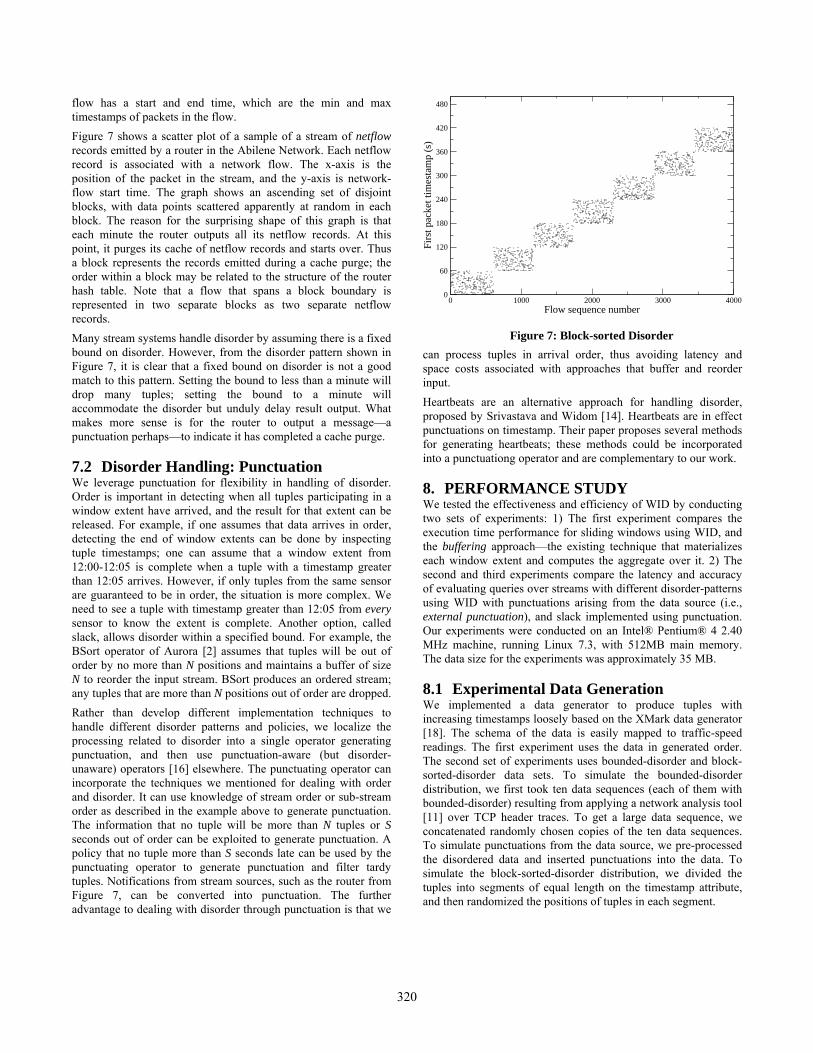
flow has a start and end time, which are the min and max timestamps of packets in the flow. Figure 7 shows a scatter plot of a sample of a stream of netflow records emitted by a router in the Abilene Network. Each netflow record is associated with a network flow. The x-axis is the position of the packet in the stream, and the y-axis is network-flow start time. The graph shows an ascending set of disjoint blocks, with data points scattered apparently at random in each block. The reason for the surprising shape of this graph is that each minute the router outputs all its netflow records. At this point, it purges its cache of netflow records and starts over. Thus a block represents the records emitted during a cache purge; the order within a block may be related to the structure of the router hash table. Note that a flow that spans a block boundary is represented in two separate blocks as two separate netflow records. Many stream systems handle disorder by assuming there is a fixed bound on disorder. However, from the disorder pattern shown in Figure 7, it is clear that a fixed bound on disorder is not a good match to this pattern. Setting the bound to less than a minute will drop many tuples; setting the bound to a minute will accommodate the disorder but unduly delay result output. What makes more sense is for the router to output a message—a punctuation perhaps—to indicate it has completed a cache purge.

7.2 Disorder Handling: Punctuation We leverage punctuation for flexibility in handling of disorder. Order is important in detecting when all tuples participating in a window extent have arrived, and the result for that extent can be released. For example, if one assumes that data arrives in order, detecting the end of window extents can be done by inspecting tuple timestamps; one can assume that a window extent from 12:00-12:05 is complete when a tuple with a timestamp greater than 12:05 arrives. However, if only tuples from the same sensor are guaranteed to be in order, the situation is more complex. We need to see a tuple with timestamp greater than 12:05 from every sensor to know the extent is complete. Another option, called slack, allows disorder within a specified bound. For example, the BSort operator of Aurora [2] assumes that tuples will be out of order by no more than N positions and maintains a buffer of size N to reorder the input stream. BSort produces an ordered stream; any tuples that are more than N positions out of order are dropped. Rather than develop different implementation techniques to handle different disorder patterns and policies, we localize the processing related to disorder into a single operator generating punctuation, and then use punctuation-aware (but disorder-unaware) operators [16] elsewhere. The punctuating operator can incorporate the techniques we mentioned for dealing with order and disorder. It can use knowledge of stream order or sub-stream order as described in the example above to generate punctuation. The information that no tuple will be more than N tuples or S seconds out of order can be exploited to generate punctuation. A policy that no tuple more than S seconds late can be used by the punctuating operator to generate punctuation and filter tardy tuples. Notifications from stream sources, such as the router from Figure 7, can be converted into punctuation. The further advantage to dealing with disorder through punctuation is that we

can process tuples in arrival order, thus avoiding latency and space costs associated with approaches that buffer and reorder input. Heartbeats are an alternative approach for handling disorder, proposed by Srivastava and Widom [14]. Heartbeats are in effect punctuations on timestamp. Their paper proposes several methods for generating heartbeats; these methods could be incorporated into a punctuationg operator and are complementary to our work.

8. PERFORMANCE STUDY We tested the effectiveness and efficiency of WID by conducting two sets of experiments: 1) The first experiment compares the execution time performance for sliding windows using WID, and the buffering approach—the existing technique that materializes each window extent and computes the aggregate over it. 2) The second and third experiments compare the latency and accuracy of evaluating queries over streams with different disorder-patterns using WID with punctuations arising from the data source (i.e., external punctuation), and slack implemented using punctuation. Our experiments were conducted on an Intel® Pentium® 4 2.40 MHz machine, running Linux 7.3, with 512MB main memory. The data size for the experiments was approximately 35 MB.

8.1 Experimental Data Generation We implemented a data generator to produce tuples with increasing timestamps loosely based on the XMark data generator [18]. The schema of the data is easily mapped to traffic-speed readings. The first experiment uses the data in generated order. The second set of experiments uses bounded-disorder and block-sorted-disorder data sets. To simulate the bounded-disorder distribution, we first took ten data sequences (each of them with bounded-disorder) resulting from applying a network analysis tool [11] over TCP header traces. To get a large data sequence, we concatenated randomly chosen copies of the ten data sequences. To simulate punctuations from the data source, we pre-processed the disordered data and inserted punctuations into the data. To simulate the block-sorted-disorder distribution, we divided the tuples into segments of equal length on the timestamp attribute, and then randomized the positions of tuples in each segment.

0 1000 2000 3000 4000Flow sequence number

0

60

120

180

240

300

360

420

480

Firs

t pac

ket t

imes

tam

p (s

)

Figure 7: Block-sorted Disorder

320

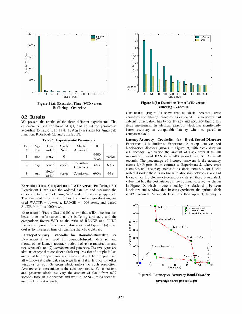
Figure 8 (b): Execution Time: WID versus Buffering – Zoom-in

8.2 Results We present the results of the three different experiments. The experiments used variations of Q1, and varied the parameters according to Table 1. In Table 1, Agg Fcn stands for Aggregate Function, R for RANGE and S for SLIDE.

Table 1: Experimental Parameters

Exp#

Agg Fcn

Dis-order

Slack Size

Slack Approach

R S

1 max none 0 4000rows varies

2 avg bound varies Consistent Generous 64 s 6.4 s

3 cnt block-sorted varies Consistent 600 s 60 s

Execution Time Comparison of WID versus Buffering: For Experiment 1, we used the ordered data set and measured the execution time cost of using WID and the buffering approach. The measured time is in ms. For the window specification, we used WATTR = row-num, RANGE = 4000 rows, and varied SLIDE from 1 to 4000 rows. Experiment 1 (Figure 8(a) and (b)) shows that WID in general has better time performance than the buffering approach, and the comparison favors WID as the ratio of RANGE and SLIDE increases. Figure 8(b) is a zoomed-in version of Figure 8 (a); scan cost is the measured time of scanning the whole data set.

Latency-Accuracy Tradeoffs for Bounded-Disorder: For Experiment 2, we used the bounded-disorder data set and measured the latency-accuracy tradeoff of using punctuation and two types of slack [2]: consistent and generous. The two types are similar, except that consistent slack requires that if a tuple is late and must be dropped from one window, it will be dropped from all windows it participates in, regardless if it is late for the other windows or not. Generous slack makes no such restriction. Average error percentage is the accuracy metric. For consistent and generous slack, we vary the amount of slack from 0.32 seconds through 3.2 seconds and we use RANGE = 64 seconds, and SLIDE = 64 seconds.

Our results (Figure 9) show that as slack increases, error decreases and latency increases, as expected. It also shows that external punctuation has better latency and accuracy than either slack mechanism. In addition, generous slack has significantly better accuracy at comparable latency when compared to consistent slack.

Latency-Accuracy Tradeoffs for Block-Sorted-Disorder: Experiment 3 is similar to Experiment 2, except that we used block-sorted disorder (shown in Figure 7), with block duration 490 seconds. We varied the amount of slack from 0 to 600 seconds and used RANGE = 600 seconds and SLIDE = 60 seconds. The percentage of incorrect answers is the accuracy metric for Figure 10. In contrast to Experiment 2, where error decreases and accuracy increases as slack increases, for block-sorted disorder there is no linear relationship between slack and latency. For the block-sorted-disorder data set there is one slack value that has the best latency, at the optimal accuracy, as shown in Figure 10, which is determined by the relationship between block size and window size. In our experiment, the optimal slack is 491 seconds. When slack is less than optimal, latency is

Figure 8 (a): Execution Time: WID versus Buffering – Overview

Figure 9: Latency vs. Accuracy Band-Disorder (average error percentage)

321

essentially independent of slack. As slack increases above the optimal, latency jumps dramatically. In this case, it would be difficult to use slack to tune the latency and accuracy of the query, as one might hope to do. It also shows that external punctuation has better latency and accuracy for block-sorted disorder than any slack amount used.

9. CONCLUSION AND DISCUSSION We believe that the work here makes three important contributions to the field of data-stream processing: 1) a framework for defining window semantics independent of any particular operator implementation algorithm; 2) a one-pass query evaluation technique for many types of sliding-window aggregates, which generally reduces memory space usage and is very flexible in handling disorder; 3) an initial investigation on the source and nature of naturally occurring disorder in data streams, and its effects on stream system performance with different disorder-handling strategies. We believe that both our framework for window semantics and query-evaluation approach are scalable and flexible enough to be extended beyond window aggregates. In the future, we plan to apply them on window join and multi-query window aggregates.

10. ACKNOWLEDGEMENTS We thank Ted Johnson for information on sources of disorder, Abilene for giving us access to their data, and our reviewers for insightful comments. This work was supported by NSF grant IIS 0086002.

11. REFERENCES [1] The Abilene Observatory.

http://abilene.internet2.edu/observatory. [2] Abadi, D., Carney, D., Çetintemel, U., Cherniack, M.,

Convey, C., Lee, S., Stonebraker, M., Tatbul, N., Zdonik, S. Aurora: a new model and architecture for data stream management. The VLDB Journal, 12, 2 (August 2003).

[3] Arasu, A., Babu, S. and Widom, J. The CQL Continuous Query Language: Semantic Foundations and Query

Execution. Stanford University Technical Report, October 2003.

[4] Babcock, B., Babu, S., Datar, M., Motwani, R., and Widom, J. Models and Issues in Data Stream Systems. In Proc. of the 2002 ACM Symp. on Principles of Database Systems (PODS 2002), (Madison, Wisconsin, June 2002).

[5] Cranor, C., Johnson, T., Spatashek, O. Gigascope: A Stream Database for Network Applications. In Proceedings of the 2003 ACM SIGMOD International Conference on the Management of Data (SIGMOD 2003) (San Diego, CA, June 2003).

[6] Gray, J., Chaudhuri, S., Bosworth, A., Layman, A., Reichart, D., Venkatrao, M., Pellow, F., and Pirahesh, H. Cube: A Relational Aggregation Operator generalizing Group-by, Cross-Tab, and Sub-Totals. Data Mining and Knowledge Discovery 1, 1 (May 1997).

Figure 10: Latency vs. Accuracy Block-Sorted-Disorder (percentage of incorrect answer)

[7] Hammad, M., Aref, W., Franklin, M., Mokbel, M., and Elmagarmid, A.K. Efficient Execution of Sliding Window Queries over Data Streams. Purdue University Department of Computer Sciences Technical Report Number CSD TR 03-035, December 2003.

[8] Hammad, M., Franklin, M., Aref, W., and Elmagarmid, A. Scheduling for shared window joins over data streams. In Proceedings of the 29th International Conference on Very Large Databases (VLDB 2003) (September 2003, Berlin, Germany).

[9] Jin Li, David Maier, Kristin Tufte, Vassilis Papadimos, and

Peter A. Tucker. No Pane, No Gain: Efficient Evaluation of Sliding-Window Aggregates over Data Streams. In SIGMOD Record, 34, 1 (March 2005).

[10] Naughton, J., DeWitt, D., Maier, D. et al. The Niagara Internet Query System. http://www.cs.wisc.edu/niagara.

[11] Passive Measurement and Analysis project. San Diego Supercomputer Center. http://pma.nlanr.net/PMA.

[12] Radiation Detection Center, Lawrence Livermore National Lab. http://rdc.llnl.gov.

[13] Raman, V., Raman, B., Hellerstein, J.M. Online Dynamic Reordering for Interactive Data Processing. In Proceedings of the 25th International Conference on Very Large Databases (VLDB 1999) (September 1999, Edinburgh, Scotland, UK).

[14] Srivastava, U, Widom, J. Flexible Time Management in Data Stream Systems. Technical Report 2003-40, Stanford University, Stanford, CA (July 2003).

[15] Stanford Stream Query Repository. http://www-db.stanford.edu/stream/sqr.

[16] Tucker, P., Maier, D., Sheard, T. and Fegaras, L. Exploiting Punctuation Semantics in Continuous Data Streams. Transactions on Knowledge and Data Engineering, 15, 3 (May 2003).

[17] Urhan, T. and Franklin, M. J. Dynamic Pipeline Scheduling for Improving Interactive Query Performance. In Proceedings of 27th International Conference on Very Large Data Bases (VLDB 2001) (September 2001, Rome, Italy).

[18] XMark Benchmark. http://www.xml-benchmark.org

322