Semantic)Comparison)of)Structured) Visual)Dataflow…anh/images/ADang.pdf ·...
94
Semantic Comparison of Structured Visual Dataflow Programs by Dang Tuan Anh Submitted in partial fulfilment of the requirements for the degree of Master of Computer Science at Dalhousie University Halifax, Nova Scotia December 2009 © Copyright by Dang Tuan Anh, 2009
Transcript of Semantic)Comparison)of)Structured) Visual)Dataflow…anh/images/ADang.pdf ·...
Semantic Comparison of Structured Visual Dataflow Programs
by
Dang Tuan Anh
Submitted in partial fulfilment of the requirements for the degree of Master of Computer Science
at
Dalhousie University Halifax, Nova Scotia December 2009
© Copyright by Dang Tuan Anh, 2009
ii
DALHOUSIE UNIVERSITY
FACULTY OF COMPUTER SCIENCE
The undersigned hereby certify that they have read and recommend to the Faculty of
Graduate Studies for acceptance a thesis entitled “Semantic Comparison of Structured
Visual Dataflow Programs” by Dang Tuan Anh in partial fulfilment of the requirements
for the degree of Master of Computer Science.
Dated: December 04, 2009
Supervisor: _________________________________
Readers: _________________________________
_________________________________
_________________________________

iii
DALHOUSIE UNIVERSITY
DATE: December 04, 2009
AUTHOR: Dang Tuan Anh
TITLE: Semantic Comparison of Structured Dataflow Programs
DEPARTMENT OR SCHOOL: Computer Science
DEGREE: MCS CONVOCATION: May YEAR: 2010
Permission is herewith granted to Dalhousie University to circulate and to have copied for non-commercial purposes, at its discretion, the above title upon the request of individuals or institutions.
_______________________________ Signature of Author
The author reserves other publication rights, and neither the thesis nor extensive extracts from it may be printed or otherwise reproduced without the author’s written permission. The author attests that permission has been obtained for the use of any copyrighted material appearing in the thesis (other than the brief excerpts requiring only proper acknowledgement in scholarly writing), and that all such use is clearly acknowledged.
iv
Table of Content
LIST OF TABLES................................................................................................. VI
LIST OF FIGURES..............................................................................................VII
ABSTRACT ........................................................................................................ VIII
LIST OF ABBREVIATION AND SYMBOLS USED ....................................... IX
ACKNOWLEDGEMENT ..................................................................................... X
CHAPTER 1: INTRODUCTION ............................................................................... 1
1.1 The evolution of visual languages............................................................... 1
1.2 The use of visual tools in software engineering.......................................... 2
1.2.1 CASE tools ......................................................................................... 3
1.2.2 UML.................................................................................................... 4
1.2.3 Other tools........................................................................................... 4
1.3 Visual Programming Languages? ............................................................... 6
1.3.1 Prograph.............................................................................................. 7
1.3.2 LabVIEW............................................................................................ 8
1.3.3 VEE..................................................................................................... 8
1.3.4 Simulink.............................................................................................. 9
1.4 Motivation for research ............................................................................. 10
CHAPTER 2: BACKGROUND ............................................................................... 12
2.1 Software development support tools for TPLs.......................................... 12
2.2 Differencing in TPLs................................................................................. 12
2.3 Differencing in DVPLs ............................................................................. 19
CHAPTER 3: EQUIVALENCE OF DATA FLOW PROGRAMS .................................. 23
CHAPTER 4: COMPARISON ALGORITHM ........................................................... 28
4.1 Counting differences ................................................................................. 28
4.2 The comparison algorithm ........................................................................ 32
4.2.1 Further optimisation of the search .................................................... 36
4.2.2 Practical issues .................................................................................. 37
4.2.3 Correctness and performance............................................................ 38
v
CHAPTER 5: EXPERIMENTAL RESULTS AND EVALUATION ............................... 42
5.1 Algorithm performance in deeply-nested structure programs................... 43
5.2 Using sub-graph isomorphism for methods with large number of operations in their diagrams ...................................................................... 44
CHAPTER 6: CONCLUSIONS AND FUTURE RESEARCH ....................................... 46
6.1 Conclusions ............................................................................................... 46
6.2 Future work ............................................................................................... 47
BIBLIOGRAPHY.................................................................................................... 50
APPENDIX A ....................................................................................................... 54
APPENDIX B ....................................................................................................... 71
vi
List of Tables
Table 5-1. Two very large programs for experiments................................................... 42
Table 5-2. Experiment test data..................................................................................... 43
Table 5-3. Testing non-equivalent methods .................................................................. 44
Table 5-4. Testing non-equivalent methods with large numbers of operations in their cases ............................................................................................................. 44
vii
List of Figures
Figure 1-1 Hieroglyphics [1] ............................................................................................. 1
Figure 1-2 User Registration Data Flow Chart [4] ............................................................ 3
Figure 1-3 X-Tango animation of the quicksort algorithm [10]........................................ 4
Figure 1-4 Visualizing the age of program code changes [10].......................................... 5
Figure 1-5 Prograph method quicksort .............................................................................. 7
Figure 1-6 A sample program of LabVIEW...................................................................... 8
Figure 1-7 A VEE program to find maximum elements in an array [23].......................... 9
Figure 1-8 A Simulink program for simulating the motion of a bouncing ball [2] ........... 9
Figure 2-1 A simple program with one main procedure and its corresponding PDG ..... 15
Figure 2-2 A program with two procedures and its corresponding SDG ........................ 17
Figure 2-3 Prograph comparison tool .............................................................................. 20
Figure 2-4 LabVIEW VIs comparison............................................................................. 21
Figure 2-5 SimDiff comparison models [50]................................................................... 22
Figure 3-1 Isomorphic graphs that violate equivalence conditions ................................. 25
Figure 4-1 What are the differences?............................................................................... 28
Figure 4-2 Counting differences between operations ...................................................... 29
Figure 4-3 Directed acyclic graphs corresponding to the cases in Figure 3-1................. 30
Figure 4-4 The search tree structure. Counts of square nodes can only decrease during search, and Counts of circular ones can only increase................................... 33
Figure 4-5 (1) Search down a path stops at a node X with no children. (2) Cut-off occurs when C(Y) becomes 0.................................................................................... 35
Figure 4-6 The value alpha(Y) used to cut off search in step 5 is inherited from node Z via steps 2 to 4................................................................................................ 36
Figure 4-7 The search tree structure. Counts of square nodes can only decrease during search, and Counts of circular ones can only increase................................... 37
Figure 4-8 Search below the node consisting of these two cases will terminate since there are no subgraph isomorphisms....................................................................... 41
Figure 4-9 The algorithm determines that methods fact-a and fact-b are semantically equivalent ....................................................................................................... 41
viii
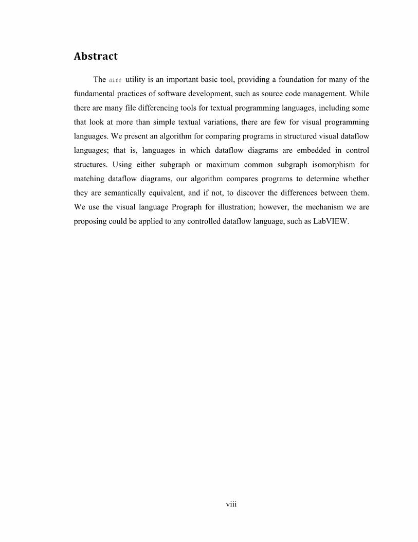
Abstract
The diff utility is an important basic tool, providing a foundation for many of the
fundamental practices of software development, such as source code management. While
there are many file differencing tools for textual programming languages, including some
that look at more than simple textual variations, there are few for visual programming
languages. We present an algorithm for comparing programs in structured visual dataflow
languages; that is, languages in which dataflow diagrams are embedded in control
structures. Using either subgraph or maximum common subgraph isomorphism for
matching dataflow diagrams, our algorithm compares programs to determine whether
they are semantically equivalent, and if not, to discover the differences between them.
We use the visual language Prograph for illustration; however, the mechanism we are
proposing could be applied to any controlled dataflow language, such as LabVIEW.
ix
List of Abbreviation and Symbols used
VL Visual Language
GUI Graph User Interface
IDE Integrated Development Environment
CASE Computer-Aided Software Engineering
UML Unified Modelling Language
VPL Visual Programming Language
DVPL Dataflow Visual Programming Language
SVPL Structured Dataflow Visual Programming Language
TPL Textual Programming Language
PDG Program Dependence Graph
SDG System Dependence Graph
PRG Program Representation Graph
VI Virtual Instruments
MCS Maximum Common Subgraph

x
Acknowledgement
I would like to express my deep gratefulness to Dr. Phil Cox for helping me finish
this thesis. He has always encouraged and shown much patience for my thesis research
and spent a lot of time reviewing and giving valuable suggestions from detecting very
slight writing style errors to suggesting innovative ideas. I have studied a lot since
working with him in my Master thesis for both academic research and personal
development.
Thank you to Dr. Arthur Sedgwick and Dr. Brad Lushman for being members of
the examining committee.
I would like to thank Simon Gauvin for his help on the implementation part of this
thesis.
Finally, I would like to thank my wife Yen Le for her support and encouragement
during my study.
1
Chapter 1: Introduction
1.1 The evolution of visual languages
A Visual Language (VL) refers to a way of using images and diagrams for
communication purposes. VLs have been used since the dawn of human history. In
ancient times, words and images already played an important role in communication
between people. They often used cave paintings to express their thoughts in simple
sketches and drawings. The ancients also exploited images in the use of languages, such
as pictographs, ideograms, phonograms, and hieroglyphics [1]. In these languages, each
graphic symbol can be referred directly or indirectly. For example, Figure 1-1 shows an
example of ideogram to represent, “to eat” or “to drink”.
Figure 1-1 Hieroglyphics [1]
Although VLs have had a long history, they reached their turning point with the
advent of low-cost graphic computers. In 1983, with the introduction of Macintosh
computers by Apple Computer Inc., people could communicate with a computer by a
mouse, keyboard, and graphical user interface instead of a simple command-line
interface. More importantly, Macintosh computers provided an ability to integrate the use
of diagrams and images for communication. For computer users, some obvious benefits
of this innovation were that users could delete a file or folder by dragging to the trash,
rename files, or move files.
Although diagrams, such as Goldstine and von Neumann flow diagrams, PERT and
CPM Charts [1], were already being used at this time, they were mainly paper-based. As
the popularity of graphic user interfaces (GUI) for personal computers increased,
researchers began to investigate the benefits of images and diagrams in computer
software development. Unfortunately, software developers had to continue using text
languages to write complex software programs and develop GUI programming. In an
effort to resolve this shortcoming, there was great interest in exploring the direct use of
diagrams in software development. The advent of graphic computers and the lack of
2
adequate development tools led to intensive research on visual tools for software
development, such as visual software project management tools, integrated development
environments (IDEs), and visual tools for software modelling and engineering [2].
1.2 The use of visual tools in software engineering
Today, the demand for software applications is increasing at an astounding rate.
They are used in many areas, including aerospace, nuclear power generation, financial
markets and so on. A virtual army of programmers, designers, and project managers are
employed in the computer industry. However, software development is an intricate
process requiring the combination of many disciplines from modelling and design to code
generation, project management, testing, deployment, change management, and beyond
[3]. In the software design phase, designers need to analyze and understand customer
requirements from purely textual descriptions. A good design plan helps developers to
understand project requirements in the coding phase. Nevertheless, not all software
requirements can be expressed efficiently in textual languages in order, for instance, to
display the relationship between database elements or draw electronic circuits.
Additionally, a software project can involve many developers for many years. Over the
years, such a project can include millions of lines of code. The enormous size of software
programs, together with a lack of well designed documentation leads to the problem that
understanding, analyzing, changing, and modifying code is extremely time-consuming
and costly.
In order to produce a reliable product at minimum cost, one approach to assist
software engineers in coping with program complexity and increase programmer
productivity is the use of visualization tools. Software visualization tools take advantage
of graphical techniques to build a visual representation of the structure and behaviour of a
program. Software structure is intricate and challenging to understand, so these
visualization tools aid both designers and programmers to understand and clarify
software products. The ultimate goal of visual tools is to aid the comprehension of
software systems and improve the productivity of the software development process.
In recent years, as the size and complexity of software projects has increased,
visualization tools have become very important for the software development process. A
3
wide variety of software visual tools supporting software development in accordance
with user needs and targets has been developed.
1.2.1 CASE tools
Since the beginning of computing, one of the principal efforts to improve the
software development process has been to alleviate the intervention of the human effort
in the software development cycle. This aim is achieved by applying computer-aided
software engineering (CASE) as a visualization tool to ease the specification, design,
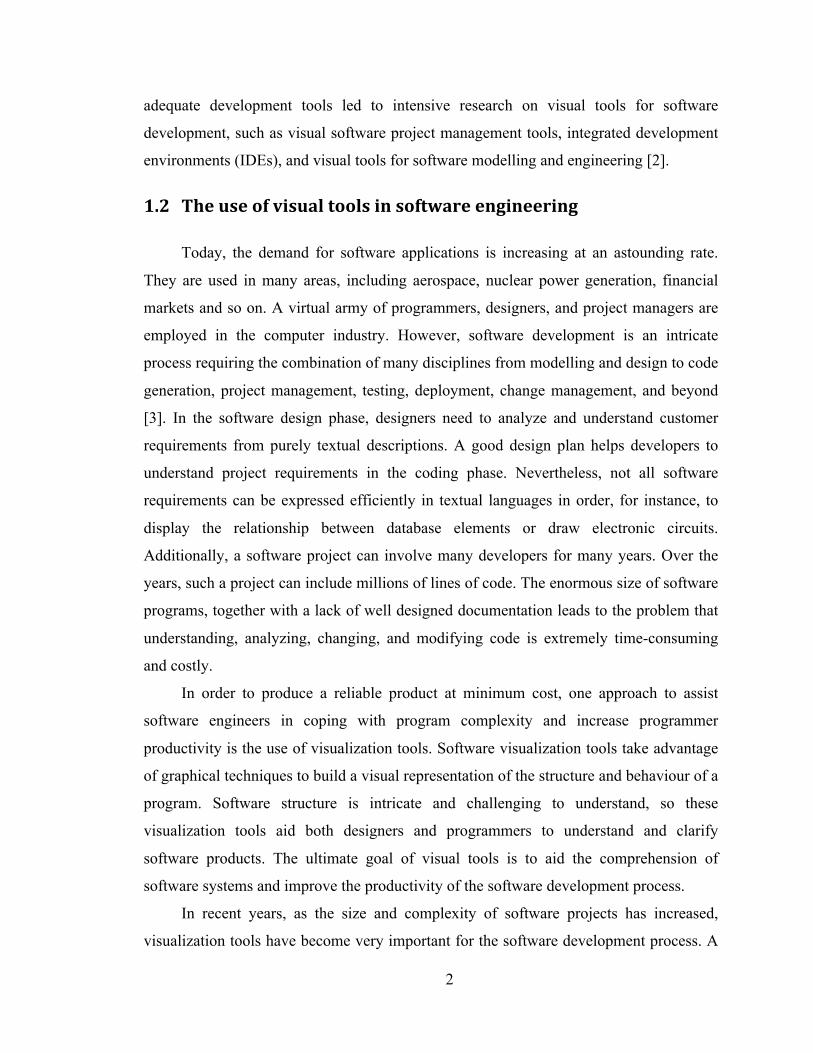
implementation and management of the software process. One typical example of
visualization CASE tools is VisualCase [4]. Figure 1-2 depicts a user registration process
by the flow chart diagram. CASE tools can also be used to visualize software
maintenance processes, data modelling tools, and database relationships.
Figure 1-2 User Registration Data Flow Chart [4]

4
1.2.2 UML
Unified Modeling Language (UML) is widely accepted as a standard for the
general-purpose modeling of software systems in the field of software engineering. UML
uses a set of graphical notations to visualize all phases of software development. For
example, EJB and Java™ UML visual editing [5] supports the capacity to visualize class
diagrams in Java. Visual Paradigm SDE for Visual Studio [6] provides a set of tools to
build a visualization of database modelling, requirement modelling, and object-relation
mapping.
1.2.3 Other tools
Mili and Steiner [7] discuss two software visualization tools named “Jinsight” and
“GraphViz”. Jinsight visualizes “the dynamic behaviour of Java programs” and allows
the user to visualize and analyze the performance and understandability of Java programs
through an execution view, object histogram view, or table view [8]. Graphviz displays
structure information through diagrams and graph networks [9].
Figure 1-3 X-Tango animation of the quicksort algorithm [10]
5
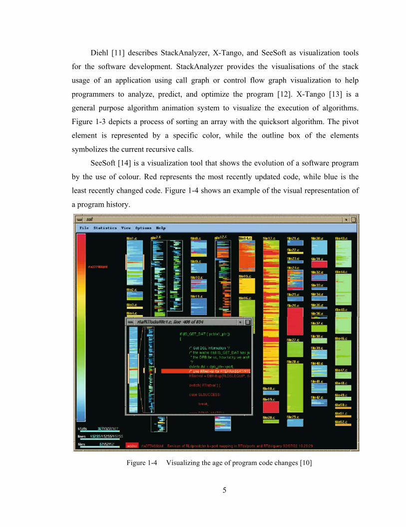
Diehl [11] describes StackAnalyzer, X-Tango, and SeeSoft as visualization tools
for the software development. StackAnalyzer provides the visualisations of the stack
usage of an application using call graph or control flow graph visualization to help
programmers to analyze, predict, and optimize the program [12]. X-Tango [13] is a
general purpose algorithm animation system to visualize the execution of algorithms.
Figure 1-3 depicts a process of sorting an array with the quicksort algorithm. The pivot
element is represented by a specific color, while the outline box of the elements
symbolizes the current recursive calls.
SeeSoft [14] is a visualization tool that shows the evolution of a software program
by the use of colour. Red represents the most recently updated code, while blue is the
least recently changed code. Figure 1-4 shows an example of the visual representation of
a program history.
Figure 1-4 Visualizing the age of program code changes [10]
6
1.3 Visual Programming Languages
In this section, we give a general overview of what Visual Programming Languages
(VPLs), explain briefly how they function and give brief descriptions of some
contemporary VPLs, both general-purpose and domain-specific. Although visual tools
already play a crucial role in software development, in the coding phase, developers still
need to deal with the complexity of programs coded in textual programming languages
(TPLs). In an effort to alleviate the complexity of programming tasks, researchers have
investigated the direct use of graphics in programming tasks called “Visual
Programming” or “Graphical Programming” [15]. There has been a recent explosion of
interest in VPLs, and some visual programming systems have been remarkably successful
in both the software industry and academic research [16,17]. The main difference
between VPLs and software visualization is their intended goal: VPLs aim to make
programming tasks easier by using graphical notation to build programs, while software
visualization strives to help programmers cope with program complexity.
A VPL is a programming language that uses a wide variety of visual symbols, such
as “spatial relationship”, icons, or shading to represent the structure of a program, so that
the programmer can have a better understanding of the program he or she is building. In
VPLs, text does not play an important role except for comments, names of entities, or
variable values. A VPL program is not necessarily translated into text at any time,
including when compiling or debugging [2], as translating to text is redundant since the
VPL by itself provides all the necessary expressive power. Research have shown that for
many tasks VPLs outperform TPLs because a visual representation of program structure
helps software developers to analyze, code, debug, and manage programs [2,18].
Although some programming languages, like Visual C++ [19] or Visual J++ [20], appear
to be similar to VPLs, they are, in fact, not VPLs. Those TPLs only take advantage of
graphical techniques and visualization to ease programmer programming tasks, not to use
visual notations to construct programs directly [10]. Some examples of VPLs are
Prograph [21], LabVIEW [16], Simulink [22] and VEE [23].
7
1.3.1 Prograph
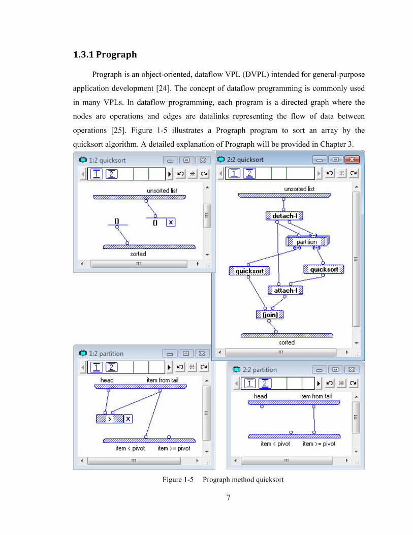
Prograph is an object-oriented, dataflow VPL (DVPL) intended for general-purpose
application development [24]. The concept of dataflow programming is commonly used
in many VPLs. In dataflow programming, each program is a directed graph where the
nodes are operations and edges are datalinks representing the flow of data between
operations [25]. Figure 1-5 illustrates a Prograph program to sort an array by the
quicksort algorithm. A detailed explanation of Prograph will be provided in Chapter 3.
Figure 1-5 Prograph method quicksort

8
1.3.2 LabVIEW
LabVIEW, a DVPL that provides libraries and a programming environment for
hardware devices, has achieved great industrial success [16]. Like Prograph, LabVIEW
can be used to program any algorithm, but the product itself is domain-specific, for
example, providing extensive support for accessing instrumentation hardware. Figure 1-6
depicts a LabVIEW program that computes the factorial of an integer. The icon “I32” at
the upper left represents the user interface control that provides the input integer, while
the constant 1 initialises the result variable. The block diagram in the centre is a “for
loop” iteration. The “for loop” variable “i” counts iterations. It begins at 0 so it will go
through the range of 0 to N-1 where N is the number of iterations.
Figure 1-6 A sample program of LabVIEW
1.3.3 VEE
VEE is another DVPL and development environment used with data acquisition
devices, such as digital voltmeters and oscilloscopes, and source devices like arbitrary
waveform generators and power suppliers. Figure 1-7 is a VEE program to find the
maximum number in an array. The “Random_Number” function generates ten random
numbers and adds them to the “Collector-Create Array”. Then the function “max(x)”
finds the maximum value in the array and displays the “Max Value” [23].

9
Figure 1-7 A VEE program to find maximum elements in an array [23]
1.3.4 Simulink
Simulink is a domain-specific dataflow visual programming environment for
simulating dynamic and embedded systems [22]. Figure 1-8 depicts a Simulink program
that simulates “the motion of a bouncing ball by continuously re-computing its velocity
and position” [2].
Figure 1-8 A Simulink program for simulating the motion of a bouncing ball [2]
Most VPLs that have achieved some level of industrial success are based on the
data flow model, and are either domain-specific or general purpose, and structured or un-
10
structured, where a structured DVPL (SVPL), is one in which the data flow diagrams are
acyclic, enclosed in control structures of some kind, and have the single-assignment
property. Some examples are as follows.
Although Simulink, a DVPL for simulation of physical systems, provides some
control structures, it is primarily unstructured, allowing feedback loops appropriate to its
application domain [26]. LabVIEW and VEE are structured and domain-specific,
designed for data acquisition and virtual instrument control [16,23]. Prograph is
structured and general purpose [24]. During its commercial life, Prograph CPX was used
in a range of projects in which C++ would have been the usual choice [17]. At present, to
our best knowledge, it is the only visual programming environment that has been used in
this way for industrial software development, as a replacement for traditional text-based
tools. Hence, in considering software development support tools, we have focussed on
SVPLs.
1.4 Motivation for research
Although VPLs have been the subject of continuing research for at least the last 25
years, they, unlike their textual counterparts, have made few inroads into the world of
industrial software development and are not considered a part of mainstream software
engineering. While it has become the norm to use visual representations to specify the
architecture of software systems, visual representation of algorithms has not caught on as
a replacement for or a supplement to standard, imperative, TPLs. This lack of success is
at least partly due to the reluctance of professional developers to invest in learning about
a new technology [27]. However, unless the new technology satisfies certain criteria, the
professional developer should be wary of adopting it, as participants noted in a focus
group study conducted by Apple to determine the viability of Prograph CPX as a devel-
opment environment for Windows applications [28]. In particular, to become a viable
alternative to textual programming, a VPL should interoperate with standard textual
languages, by, for example, providing a robust, reversible translation between visual and
textual programs [29]; include modern language features such as exception handling [30];
and include visual counterparts of the many code management and analysis tools
available for textual languages, which is the focus of the work reported here.
11
One of the mainstays of many of the code management tools used by software de-
velopers is differencing, exemplified in its simplest form by the UNIX diff command
which finds the lexical differences between two text files or source programs. Among
other things, it is used, to manage modifications and rollback changes, reveal anomalies
during debugging, manage concurrent changes made by several people, and merge
changes from different versions of programs. Differencing underpins many source code
control systems such as CVS [31] and SVN [32]. Although there has been extensive
research on differencing algorithms for TPLs, a lack of good differencing tools is one of
the main obstacles preventing the popular use of VPLs for professional developers.
Here, we propose a differencing algorithm in VPLs to eliminate one of the
impediments to their industrial adoption. In Chapter 2, we discuss differencing in textual
software development and briefly review the existing differencing tools in VPLs. In
Chapter 3, we define semantic equivalence, an equivalence relation on program elements
in an SVPL, while in Chapter 4 we present an algorithm for finding semantic
equivalence, or discovering semantic differences. Experimental results and an evaluation
are discussed in Chapter 5. Finally, we make some concluding remarks and discuss future
work in Chapter 6.
12
Chapter 2: Background
2.1 Software development support tools for TPLs
Software development support tools, such as developing tools, analyzing tools,
testing tools, debugging tools, and maintaining tools, are programs or applications
devised to ease the tasks of software developers. When the size and complexity of
software projects increases, there is a need to develop some source-code control tools to
manage the huge amount of code. For example, the purpose of testing tools is to find
software bugs when executing programs, while debugging tools assist programmers to
locate a bug in a large program. Initially, these tools were very simplistic, but they have
since become quite complex and have been incorporated into a powerful IDE. IDEs help
to increase programmer productivity and ease programming tasks. They include some
valuable features, such as, a source-code editor, a compiler, and a debugger. Some typical
commercial IDEs are Visual Studio 2008 for .NET development and Eclipse for Java.
One other indispensable integrated feature in IDEs is differencing tools. Differencing
tools locate all the differences between two files or programs and provide information
which can then be used by other source code management tools to generate a change
history. Differencing tools also allow programmers to see the history of changes between
different versions of a program made by many developers. In the next section, we present
a brief overview of differencing tools for TPLs.
2.2 Differencing in TPLs
In TPLs, differencing tools play a vital role in finding differences between two
programs. When a software project is large and involves many software developers, the
complexity of the software program also increases. As time goes by, and new
programmers join this project to fix bugs, find discrepancies, or reveal underlying flaws
between two versions of a program, they need to analyze and understand a large amount
of code made by previous developers. This task can be very frustrating and time-
consuming. There is thus a need not only to know the changes made by other
programmers but to ease program understanding and maintenance tasks.
13
File differencing first appeared in the UNIX operating system in the early 1970s,
using an algorithm reported in Hunt and Mcllroy [33]. The seminal algorithms for the diff
command were first proposed in Miller and Myer [34,35] and Ekkonen [36]. The
traditional UNIX utility diff is designed to discover differences between text files rather
than programs. This utility is too simple to present accurate results for the differences
between two programs. Moreover, this comparison tool often produces irrelevant results;
for example, a minor difference, such as an extra space or line break can contribute sig-
nificantly to the result of a comparison, since diff looks for physical differences rather
than syntactic ones.
In response to these limitations, many syntactic diff algorithms have been
developed that build syntax trees representing the structure of programs. Comparing two
programs is equivalent to comparing their trees [37]. For instance, Cdiff uses a tree-
matching algorithm to compare syntactic differences between two programs in the C
language [38]. Syntactic algorithms can more accurately locate differences, such that
extra spaces or line breaks can be eliminated. However, syntactic comparison utilities
also have a critical shortcoming: they cannot find the semantic differences between two
programs because the comparison is entirely based on the program text and syntactic
structure [37]. One syntactic difference between two programs can result in many
semantic differences which a syntactic differencing algorithm cannot locate.
To overcome this limitation, various comparison methods have been proposed that
build structural representations of programs, allowing semantics to be taken into account.
Two such representations are program dependence graphs (PDGs) and system
dependence graphs (SDGs) which include both control and data flow information.
Binkley [39] presents an empirical study to justify the helpfulness and usefulness of
semantic differencing algorithms for the tasks of program comprehension. Semantic
differencing tools based on applying graph isomorphism to subgraphs have achieved
some level of success [40,41]. In the next paragraph, we will present some definitions of
PDGs and SDGs as discussed in Horwitz [42].
The PDG of a program is a directed graph the vertices of which represent the
assignment statements and the predicate statements, such as “if-else” or “while”. Each
PDG starts with an “ENTRY” vertex representing entrance into the procedure. The edges
14
between vertices represent either control or data dependence. Control dependence
edges, which are labelled either true or false, represent the conditional structures of
programs in TPLs, such as if-else or while structures. The source of a control dependence
edge can be the ENTRY vertex or a predicate vertex containing a condition to be tested,
while the destination of a control dependence edge can be an assignment statement that is
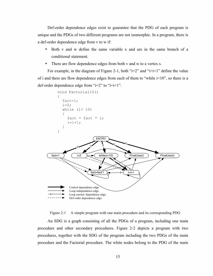
dependent on the source. Figure 2-1 depicts a program for computing the factorial of 10,
together with the PDG of the program. In the diagram, the bold arrow edge from the
vertex “while i<10” to the vertex “fact=fact*i” is a control dependence edge, indicating
that the condition “while i<10” determines whether or not the assignment statement
“fact=fact*i” is executed.
Data dependence edges include flow dependence edges and def-order
dependence edges. The flow dependence edges represent the flow of values through a
program. There is a flow dependence edge from vertex v to vertex w if:
• v defines variable x
• w uses variable x
• There is no execution path from v to w passing through a vertex that defines x.
There are two sub-types of flow dependence edges: loop independent and loop
carried edges. A flow dependence edge from v to w is carried by a loop L if:
• There is an execution path from v to w that includes a flow dependence edge
from a statement to the predicate statement of loop L.
• The statements corresponding to v and w are in the body of the loop L.
For example, in the diagram of Figure 2-1,”i= i+1” defines the value of i, while
“fact= fact*i” uses the value of i; both statements are enclosed in the loop “while i<=10”,
and there is a flow dependence edge from “i=i+1” to the predicate “while i<10”; thus,
there is a loop carried edge from “i=i+1” to “fact=fact*i”.
In contrast, if there is no flow dependence edge to the predicate statement, the data
dependence edge is called loop independent. In the diagram of Figure 2-1, statement
“fact=1” defines the variable fact, while “fact=fact*i” uses the variable fact and there is
no flow dependence edge from w or v to any predicate statement. Hence, there is a loop
independence edge from “fact=1” to “fact=fact*i”.
15
Def-order dependence edges exist to guarantee that the PDG of each program is
unique and the PDGs of two different programs are not isomorphic. In a program, there is
a def-order dependence edge from v to w if:
• Both v and w define the same variable x and are in the same branch of a
conditional statement.
• There are flow dependence edges from both v and w to a vertex s.
For example, in the diagram of Figure 2-1, both “i=2” and “i=i+1” define the value
of i and there are flow dependence edges from each of them to “while i<10”, so there is a
def-order dependence edge from “i=2” to “i=i+1”. void Factorial10() {
fact=1; i=2; while (i< 10) {
fact = fact * i; i=i+1;
} }
Figure 2-1 A simple program with one main procedure and its corresponding PDG
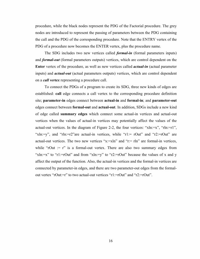
An SDG is a graph consisting of all the PDGs of a program, including one main
procedure and other secondary procedures. Figure 2-2 depicts a program with two
procedures, together with the SDG of the program including the two PDGs of the main
procedure and the Factorial procedure. The white nodes belong to the PDG of the main
fact=1 i=2
fact=fact*i
while(i<10)
i=i+1
ENTRY
FinalUse(i) FinalUse(i)
T T T T T
TT
Control dependence edgeLoop independence edgeLoop carried dependence edgeDef-order dependence edge
16
procedure, while the black nodes represent the PDG of the Factorial procedure. The grey
nodes are introduced to represent the passing of parameters between the PDG containing
the call and the PDG of the corresponding procedure. Note that the ENTRY vertex of the
PDG of a procedure now becomes the ENTER vertex, plus the procedure name.
The SDG includes two new vertices called formal-in (formal parameters inputs)
and formal-out (formal parameters outputs) vertices, which are control dependent on the
Enter vertex of the procedure, as well as new vertices called actual-in (actual parameter
inputs) and actual-out (actual parameters outputs) vertices, which are control dependent
on a call vertex representing a procedure call.
To connect the PDGs of a program to create its SDG, three new kinds of edges are
established: call edge connects a call vertex to the corresponding procedure definition
site; parameter-in edges connect between actual-in and formal-in; and parameter-out
edges connect between formal-out and actual-out. In addition, SDGs include a new kind
of edge called summary edges which connect some actual-in vertices and actual-out
vertices when the values of actual-in vertices may potentially affect the values of the
actual-out vertices. In the diagram of Figure 2-2, the four vertices: “xln:=x”, “rln:=r1”,
“xln:=y”, and “rln:=r2”are actual-in vertices, while “r1:= rOut” and “r2:=rOut” are
actual-out vertices. The two new vertices “x:=xln” and “r:= rln” are formal-in vertices,
while “rOut := r” is a formal-out vertex. There are also two summary edges from
“xln:=x” to “r1:=rOut” and from “xln:=y” to “r2:=rOut” because the values of x and y
affect the output of the function. Also, the actual-in vertices and the formal-in vertices are
connected by parameter-in edges, and there are two parameter-out edges from the formal-
out vertex “rOut:=r” to two actual-out vertices “r1:=rOut” and “r2:=rOut”.
17
void main() {
x = 10; y = 20; Factorial(x,r1); Factorial(y,r2); Print (r1); Print (r2);
}
void Factorial(int x, int r) {
r = 1; i = 2; while (i<=x){
r = r * i; i=i+1;
} }
Figure 2-2 A program with two procedures and its corresponding SDG
These graphs capture some of the semantic properties of programs, and, together
with a technique called slicing, can be used to find semantic differences between
programs [43]. A slice of a program with respect to some criterion is the set of all
r=1 i=2
r=r*i
while(i<=x)
i=i+1
Enter Factorial
FinalUse(i) FinalUse(r)
Enter main
Call Factorial(x,r1)
y=20
print(r1)
xln:=x r1:= rOut
rln:=r1
x:=rln
r:=rln
print(r2)
Call Factorial(y,r2)
x=10TTT
T T
T
TT
TT
TT T T T
T T
xln:=y r2:= rOut
rln:=r2
x:=rln
r:=rlnTT
rOut:=rT
T TTT
Control dependence edgeLoop independence edgeLoop carried dependence edgeDef-order dependence edge
Summary edgeCall, parameter-in, parameter-out
T T
18
statements that satisfy the criterion. For example, a criterion might be specified as a
subset of the program variables, in which case the slice would be the set of all statements
that could affect the value of any of these variables. Slices can be categorized as: static or
dynamic slice, backward or forward, and interprocedural or intraprocedural. A static slice
is computed without considering the program inputs, while a dynamic slice is calculated
with respect to a specific test case. A backward slice is a program slice the statements of
which are discovered by a backward traversal of PDGs starting at the statements affected
by the slicing criterion and a forward slice is similar to a backward slice, but the
statements are determined in the forward direction starting at the statements affected by
the slicing criterion. Finally, an intraprocedural consists of statements from only one
procedure and is computed from the corresponding PDG, while an interprocedural slice
consists of statements from several procedures and is computed from the SDG derived
from the program which includes these procedures. PDGs, SDGs and program slicing are
used widely in many applications, such as program debugging, program differencing,
program integration, software maintenance, and software testing. Various slicing
techniques are discussed in Tip [43] and Xu et al. [44]. Here, we focus on the use of these
techniques for finding semantic differences.
The use of PDGs and graph isomorphism to detect semantic differences has been
intensively researched. Horwitz et al. [45] state that if two PDGs of two programs are
isomorphic, the programs are strongly equivalent. Strong equivalence means that with the
same inputs, two programs will produce the same outputs.
Yang et al. [46] propose the Sequence-Congruence Algorithm using program
representation graphs (PRGs), a variant of PDGs in which extra variables are introduced
to obtain the single assignment property, for discovering program components that have
identical execution behaviours. This algorithm will detect larger equivalence classes than
those discovered by comparing slices.
Horwitz [42] proposes three algorithms to calculate both semantic and textual
differences. This technique uses PRGs and a partitioning algorithm to separate program
components into partitions so that two program components will produce equivalent
behaviours, if they are in the same partition. These algorithms have been proved to be
19
more accurate than the algorithms using program slicing because they deal with smaller
components of code than the algorithm using program slicing [43].
Horwitz et al. [45] and Binkley et al. [48] present a technique using PRGs to
determine semantic differences for integrating two versions of a program based on
comparing their intraprocedural slices for the program integration algorithm. The
algorithm integrates two modified versions A, B from a program Base by merging their
PDGs with respect to their semantic differences.
Binkley [49] proposes two algorithms using PDGs and SDGs to reduce the cost
regression testing. The cost of regression testing between two versions of programs can
be reduced by detecting the semantic differences and applying incremental regression
testing. This paper also provides an empirical study to support that semantic difference
can be used as an aid for detecting errors during debugging and regression testing.
Anderson and Teitelbaum [41] present CodeSurfer, one of the most advanced
commercial analysis tools for detecting flaws in software programs based on the
dependence–graph representation of a program. CodeSurfer uses PDGs, SDGs and
program slicing to provide a graph library for accessing to and querying on SDGs for the
purpose of software investigation and maintenance, for example, finding the dependency
between two selected statements or locating where a variable was assigned its value.
2.3 Differencing in DVPLs
One important improvement of semantic differencing tools over syntactic
differencing tools in TPLs is that the differences are defined based on program input-
output behaviours rather than syntactic changes [40]. From the perspective of structure
reflecting semantics, DVPLs have an inherent advantage over TPLs. To apply semantic
differencing techniques to programs written in the standard imperative TPLs on which
the software industry relies, the graphs that represent the semantics must first be
constructed as described above. SVPLs are functional, however, so their semantics, like
those of a functional language, are closely aligned with their syntax, a dataflow graph at
the lowest level [25]. Hence no construction phase is necessary: to compare DVPL
programs at the lowest level, we need only compare dataflow graphs. Differencing tools
are available for Prograph, LabVIEW and Simulink.
20
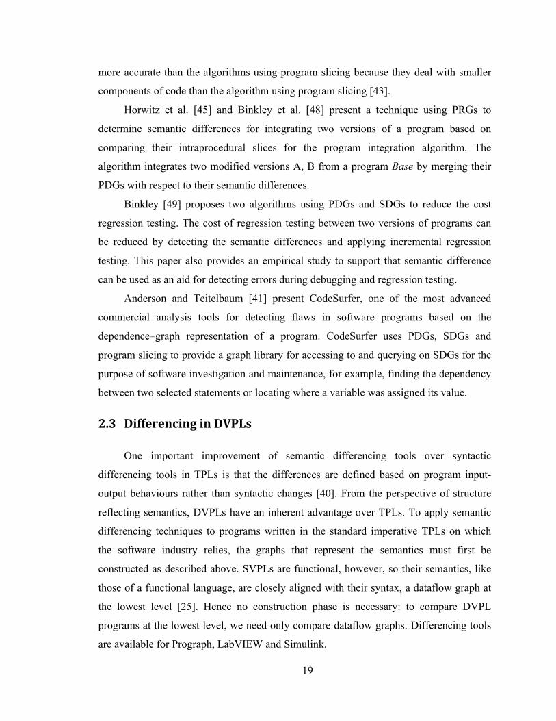
The Windows version of Prograph provides a simple file comparison tool.
However, the results show only some physical information, such as names, positions, in-
arities, out-arities, and method types. As an illustration, Figure 2-3 shows a comparison
between Prograph methods. The two windows on the top show the methods for
evaluation as highlighted, while the two windows on the bottom show the differences
between them. It is clear that these two methods have different names, positions, and in-
arity. This comparison produces only superficial syntactic differences, and does not
provide any useful information about the structural (and therefore semantic) differences
between dataflow diagrams.
Figure 2-3 Prograph comparison tool
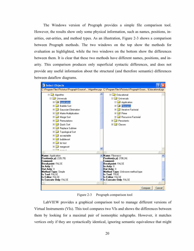
LabVIEW provides a graphical comparison tool to manage different versions of
Virtual Instruments (VIs). This tool compares two VIs and shows the differences between
them by looking for a maximal pair of isomorphic subgraphs. However, it matches
vertices only if they are syntactically identical, ignoring semantic equivalence that might
21
be determined by comparing the diagrams that implement the vertices. Hence, although it
is more sophisticated than the mechanism provided by Prograph, it is still essentially a
syntactic rather than semantic tool [16]. When the two VIs in Figure 2-4 are selected for
comparison, LabVIEW starts finding a list of differences. Figure 2-4 shows a list of
differences and their descriptions between two VIs.
Figure 2-4 LabVIEW VIs comparison
The first box lists the differences, while the second shows the details of each
difference. When we click on the “show difference” button, the selected difference detail
will be shown graphically. The diagrams of the two VIs are displayed side-by-side and
the items in the diagrams corresponding to the difference selected in the “Difference”
panel are outlined with circles as illustrated in the figure.
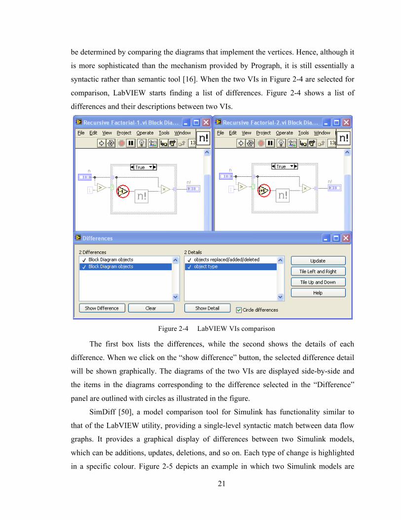
SimDiff [50], a model comparison tool for Simulink has functionality similar to
that of the LabVIEW utility, providing a single-level syntactic match between data flow
graphs. It provides a graphical display of differences between two Simulink models,
which can be additions, updates, deletions, and so on. Each type of change is highlighted
in a specific colour. Figure 2-5 depicts an example in which two Simulink models are
22
compared. SimDiff detects both cosmetic changes, for example, a simple layout change
of the two icons “Random aircraft motion” in the left of both diagrams, and syntactic
changes, for example, the kind of changes, such as inserts, deletes, updates that must be
made to transform the icon “Filter1” to the icon “Filter2”.
Figure 2-5 SimDiff comparison models [50]
Although differencing tools already play a role to some extent in VPLs, the existing
ones, described above, are quite primitive compared with those that are available for
TPLs. In the following chapters, we present a definition of equivalence for SVPLs and an
algorithm for comparing two visual dataflow programs. The relationships between
“strong equivalence”, “semantic difference” and Horwitz’s [42] algorithm, discussed
above, are analogous to the relationships between our definition of equivalence for
SVPLs, our notion of semantic difference, and the algorithm for semantic comparison of
SVPL programs.
23
Chapter 3: Equivalence of data flow programs
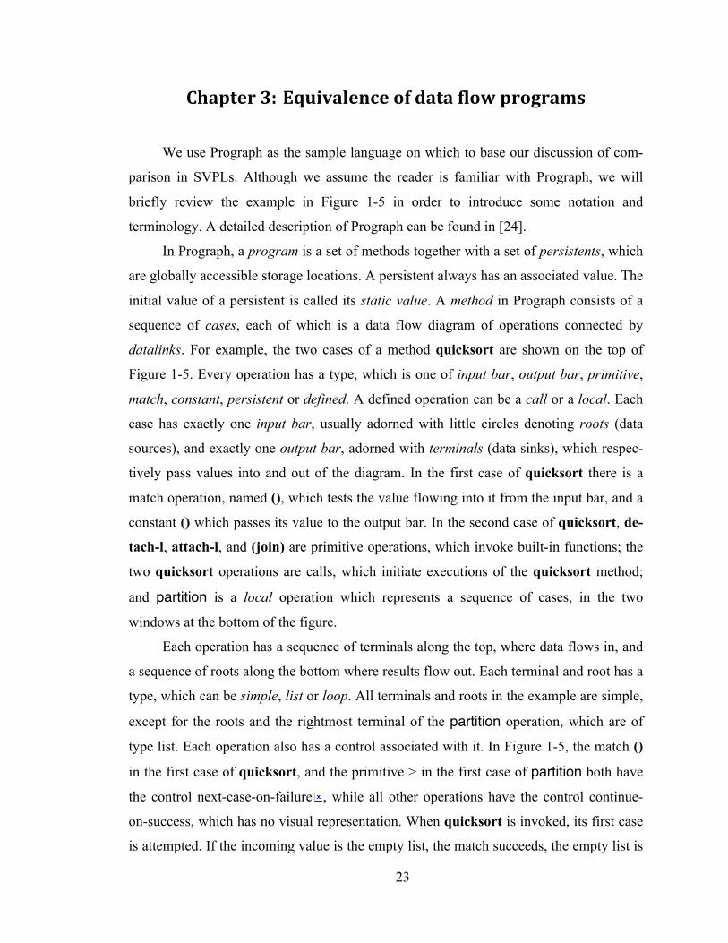
We use Prograph as the sample language on which to base our discussion of com-
parison in SVPLs. Although we assume the reader is familiar with Prograph, we will
briefly review the example in Figure 1-5 in order to introduce some notation and
terminology. A detailed description of Prograph can be found in [24].
In Prograph, a program is a set of methods together with a set of persistents, which
are globally accessible storage locations. A persistent always has an associated value. The
initial value of a persistent is called its static value. A method in Prograph consists of a
sequence of cases, each of which is a data flow diagram of operations connected by
datalinks. For example, the two cases of a method quicksort are shown on the top of
Figure 1-5. Every operation has a type, which is one of input bar, output bar, primitive,
match, constant, persistent or defined. A defined operation can be a call or a local. Each
case has exactly one input bar, usually adorned with little circles denoting roots (data
sources), and exactly one output bar, adorned with terminals (data sinks), which respec-
tively pass values into and out of the diagram. In the first case of quicksort there is a
match operation, named (), which tests the value flowing into it from the input bar, and a
constant () which passes its value to the output bar. In the second case of quicksort, de-
tach-l, attach-l, and (join) are primitive operations, which invoke built-in functions; the
two quicksort operations are calls, which initiate executions of the quicksort method;
and partition is a local operation which represents a sequence of cases, in the two
windows at the bottom of the figure.
Each operation has a sequence of terminals along the top, where data flows in, and
a sequence of roots along the bottom where results flow out. Each terminal and root has a
type, which can be simple, list or loop. All terminals and roots in the example are simple,
except for the roots and the rightmost terminal of the partition operation, which are of
type list. Each operation also has a control associated with it. In Figure 1-5, the match ()
in the first case of quicksort, and the primitive > in the first case of partition both have
the control next-case-on-failure , while all other operations have the control continue-
on-success, which has no visual representation. When quicksort is invoked, its first case
is attempted. If the incoming value is the empty list, the match succeeds, the empty list is
24
passed to the output bar and execution of quicksort concludes. Otherwise, the first case
is abandoned, and the second case tried. The head is removed from the list, and the tail
partitioned into elements that are less than the head, and those that are not. The two lists
are then sorted, and the resulting sorted list assembled and passed to the output bar.
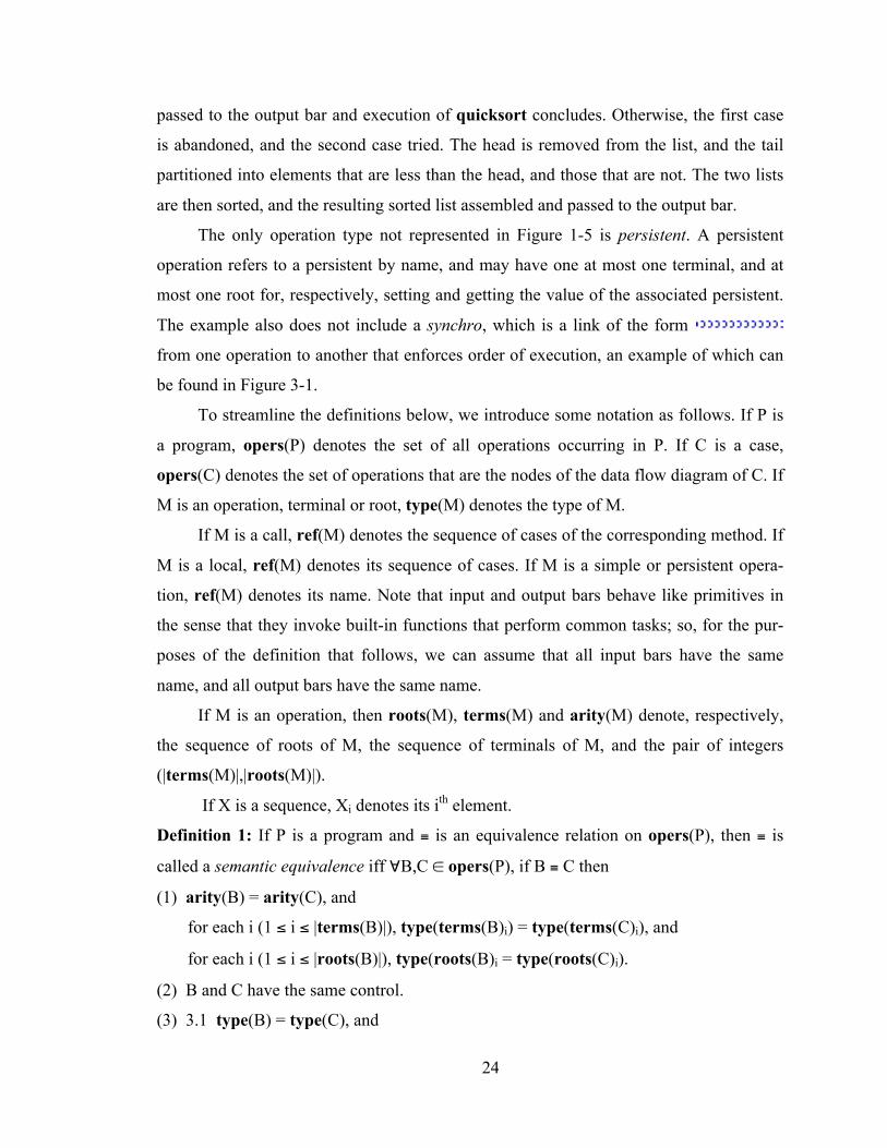
The only operation type not represented in Figure 1-5 is persistent. A persistent
operation refers to a persistent by name, and may have one at most one terminal, and at
most one root for, respectively, setting and getting the value of the associated persistent.
The example also does not include a synchro, which is a link of the form
from one operation to another that enforces order of execution, an example of which can
be found in Figure 3-1.
To streamline the definitions below, we introduce some notation as follows. If P is
a program, opers(P) denotes the set of all operations occurring in P. If C is a case,
opers(C) denotes the set of operations that are the nodes of the data flow diagram of C. If
M is an operation, terminal or root, type(M) denotes the type of M.
If M is a call, ref(M) denotes the sequence of cases of the corresponding method. If
M is a local, ref(M) denotes its sequence of cases. If M is a simple or persistent opera-
tion, ref(M) denotes its name. Note that input and output bars behave like primitives in
the sense that they invoke built-in functions that perform common tasks; so, for the pur-
poses of the definition that follows, we can assume that all input bars have the same
name, and all output bars have the same name.
If M is an operation, then roots(M), terms(M) and arity(M) denote, respectively,
the sequence of roots of M, the sequence of terminals of M, and the pair of integers
(|terms(M)|,|roots(M)|).
If X is a sequence, Xi denotes its ith element.
Definition 1: If P is a program and ≡ is an equivalence relation on opers(P), then ≡ is
called a semantic equivalence iff ∀B,C ∈ opers(P), if B ≡ C then
(1) arity(B) = arity(C), and
for each i (1 ≤ i ≤ |terms(B)|), type(terms(B)i) = type(terms(C)i), and
for each i (1 ≤ i ≤ |roots(B)|), type(roots(B)i = type(roots(C)i).
(2) B and C have the same control.
(3) 3.1 type(B) = type(C), and
25
3.2 if B is simple then ref(B) = ref(C)
3.3 else |ref(B)| = |ref(C)|, and ∀i (1 ≤ i ≤ |ref(B)|), there is
a bijection f: opers(ref(B)i) → opers(ref(C) i) such that
3.3.1. ∀A∈ opers(ref(B)i), A ≡ f(A), and
3.3.2. ∀D,E ∈ oper(ref(B)i):
(a) if there is a datalink from roots(D)j to terms(E)k for some j and k
then there is a datalink from roots(f(D))j to terms(f(E))k
(b) if there is a synchro from D to E
then there is a synchro from f(D) to f(E).
Two operations M1 and M2 in a program P are said to be semantically equivalent iff
there exists a semantic equivalence on opers(P) such that M1≡M2.
Figure 3-1 Isomorphic graphs that violate equivalence conditions
Semantic equivalence classifies operations according to what they compute. For
simple operations, this is easily determined, and depends only on the names of the op-
erations. Functionality of a defined operation is determined by the structure of the
sequence of cases to which it corresponds. The bijection between data flow diagrams
defined in 3.3 is a more constrained form of graph isomorphism. For example, condition
3.3.2(a) requires that datalinks not only connect corresponding operations in two graphs
as required for isomorphism, but also connect corresponding terminals and roots on those
operations. So although the two graphs in Figure 3-1 are isomorphic, they violate several
26
of these extra conditions: specifically, the roots of detach-l are connected to the terminals
of div in a different order, violating 3.3.2(a); the () operations have different controls,
violating 2; the operations div and div have different types, violating 3.1, and different
arities, violating 1; the show and display operations have different references, violating
3.2; and the terminals of show and display have different types, violating 1.
As noted above, the semantics of structured data flow programs, like the semantics
of functional programs and unlike those of imperative languages, is closely aligned with
the syntax. Hence, although the above definition of semantic equivalence appears to be
purely syntactic, it captures the notion of identical input/output behaviour, as does
semantic equivalence of textual programs [40]. Specifically, the relationship between
semantic equivalence and the execution functions of Prograph program elements (defined
in [17]) is characterised as follows. If P is a program A, B ∈ opers(P) and arity(A) =
arity(B) = (m,k), then A and B are semantically equivalent iff fA(w) = fB(w) for every m-
tuple w of values, where fA and fB are the execution functions of A and B, respectively.
While it can be useful to compare two operations in one program, programmers
frequently want to compare two different versions of a program. Accordingly, we need to
extend the definition of semantic equivalence. First, we note that if the two programs we
wish to compare have disjoint name spaces, and we simply combine the two programs
into one, the above relationship between semantic equivalence and Prograph execution
functions will still hold in the absence of persistents. If persistents are involved, however,
we need to ensure that there is a one-to-one correspondence between appropriate subsets
of the persistents of the two programs. Accordingly, we extend Definition 1, obtaining
the following definition, in which pers(P) denotes the set of persistents of a program P,
and value(p) and name(p) denote static value and name of a persistent p.
Definition 2: If P1 and P2 are two programs, which we can assume without loss of
generality to have no names in common, A ∈ opers(P1) and B ∈ opers(P2), then A in P1
is semantically equivalent to B in P2, denoted A[P1] ≡ B[P2] iff for some V1∈pers(P1) and
V2∈pers(P2), there is a bijection g:V1→V2 such that ∀X∈V1, value(X) = value(g(X))
and A≡B, where
• ≡ is a semantic equivalence relation on opers(P'),
• P' is the program obtained by combining P1 and P2', and

27
• P2' is obtained by renaming persistent operations in P2 as follows:
if A is a persistent operation in P2 and ref(A) = G for some G∈pers(P2)
then rename A to name(g(G)) iff G∈V2.
Note that the relationship between semantic equivalence and Prograph execution
functions also holds for this extended definition of semantic equivalence.
28
Chapter 4: Comparison algorithm
In this section, we present and discuss an algorithm, that determines whether two
methods in two programs are semantically equivalent, and if not, finds differences
between them. Note that, although Definition 1 defines semantic equivalence for
operations, it embodies as a by-product, the definition of semantic equivalence for
methods.
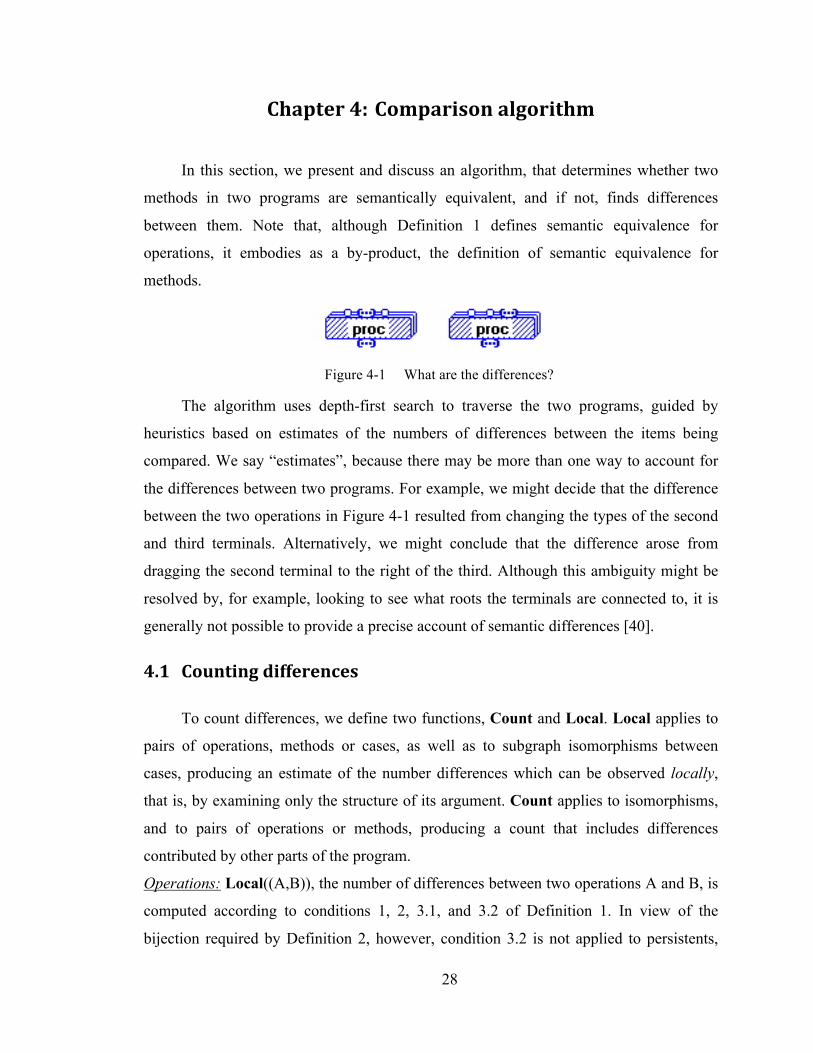
Figure 4-1 What are the differences?
The algorithm uses depth-first search to traverse the two programs, guided by
heuristics based on estimates of the numbers of differences between the items being
compared. We say “estimates”, because there may be more than one way to account for
the differences between two programs. For example, we might decide that the difference
between the two operations in Figure 4-1 resulted from changing the types of the second
and third terminals. Alternatively, we might conclude that the difference arose from
dragging the second terminal to the right of the third. Although this ambiguity might be
resolved by, for example, looking to see what roots the terminals are connected to, it is
generally not possible to provide a precise account of semantic differences [40].
4.1 Counting differences
To count differences, we define two functions, Count and Local. Local applies to
pairs of operations, methods or cases, as well as to subgraph isomorphisms between
cases, producing an estimate of the number differences which can be observed locally,
that is, by examining only the structure of its argument. Count applies to isomorphisms,
and to pairs of operations or methods, producing a count that includes differences
contributed by other parts of the program.
Operations: Local((A,B)), the number of differences between two operations A and B, is
computed according to conditions 1, 2, 3.1, and 3.2 of Definition 1. In view of the
bijection required by Definition 2, however, condition 3.2 is not applied to persistents,
29
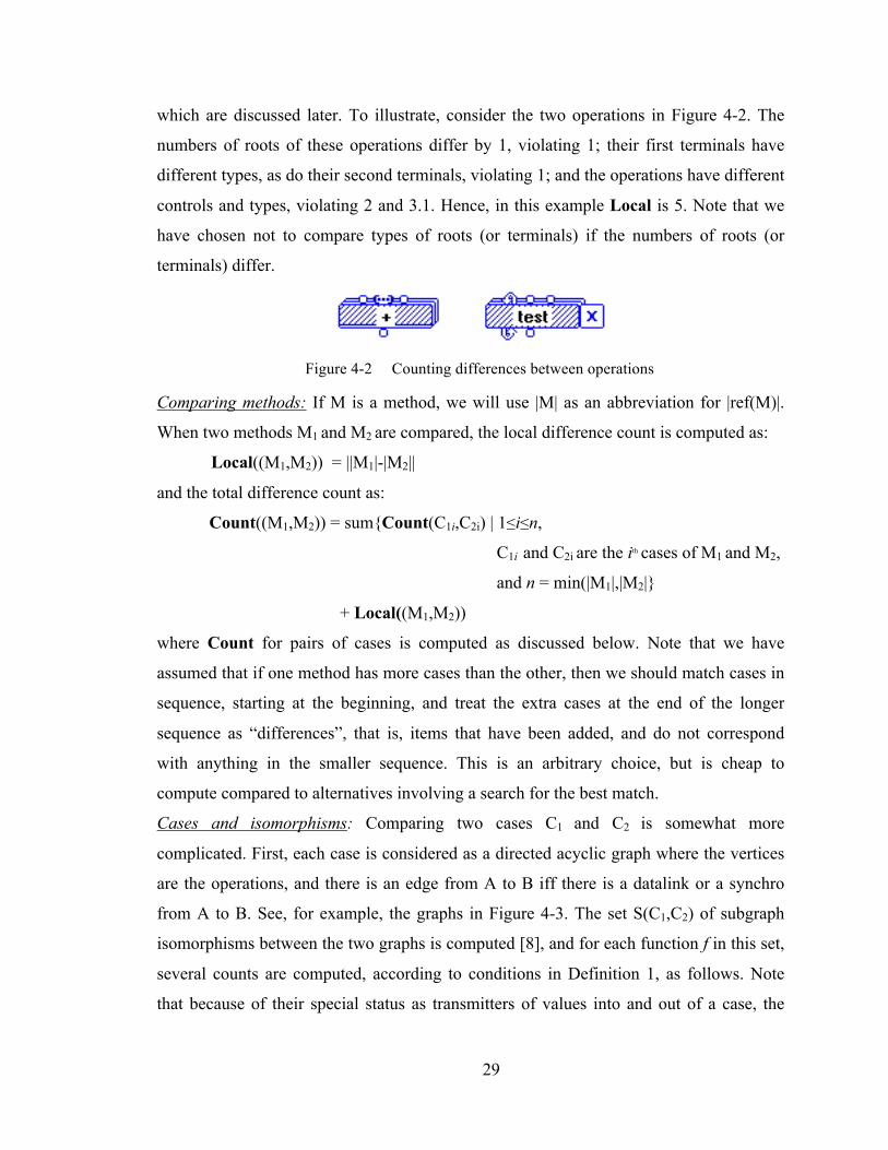
which are discussed later. To illustrate, consider the two operations in Figure 4-2. The
numbers of roots of these operations differ by 1, violating 1; their first terminals have
different types, as do their second terminals, violating 1; and the operations have different
controls and types, violating 2 and 3.1. Hence, in this example Local is 5. Note that we
have chosen not to compare types of roots (or terminals) if the numbers of roots (or
terminals) differ.
Figure 4-2 Counting differences between operations
Comparing methods: If M is a method, we will use |M| as an abbreviation for |ref(M)|.
When two methods M1 and M2 are compared, the local difference count is computed as:
Local((M1,M2)) = ||M1|-|M2||
and the total difference count as:
Count((M1,M2)) = sum{Count(C1i,C2i) | 1≤i≤n,
C1i and C2i are the ith cases of M1 and M2,
and n = min(|M1|,|M2|}
+ Local((M1,M2))
where Count for pairs of cases is computed as discussed below. Note that we have
assumed that if one method has more cases than the other, then we should match cases in
sequence, starting at the beginning, and treat the extra cases at the end of the longer
sequence as “differences”, that is, items that have been added, and do not correspond
with anything in the smaller sequence. This is an arbitrary choice, but is cheap to
compute compared to alternatives involving a search for the best match.
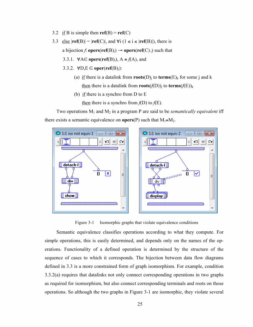
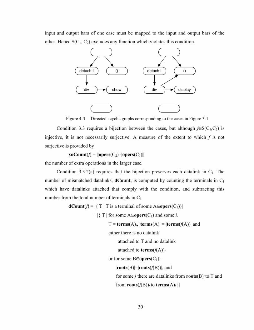
Cases and isomorphisms: Comparing two cases C1 and C2 is somewhat more
complicated. First, each case is considered as a directed acyclic graph where the vertices
are the operations, and there is an edge from A to B iff there is a datalink or a synchro
from A to B. See, for example, the graphs in Figure 4-3. The set S(C1,C2) of subgraph
isomorphisms between the two graphs is computed [8], and for each function f in this set,
several counts are computed, according to conditions in Definition 1, as follows. Note
that because of their special status as transmitters of values into and out of a case, the
30
input and output bars of one case must be mapped to the input and output bars of the
other. Hence S(C1, C2) excludes any function which violates this condition.
Figure 4-3 Directed acyclic graphs corresponding to the cases in Figure 3-1
Condition 3.3 requires a bijection between the cases, but although f∈S(C1,C2) is
injective, it is not necessarily surjective. A measure of the extent to which f is not
surjective is provided by
xoCount(f) = ||opers(C2)|-|opers(C1)||
the number of extra operations in the larger case.
Condition 3.3.2(a) requires that the bijection preserves each datalink in C1. The
number of mismatched datalinks, dCount, is computed by counting the terminals in C1
which have datalinks attached that comply with the condition, and subtracting this
number from the total number of terminals in C1.
dCount(f) = |{ T | T is a terminal of some A∈opers(C1)}|
− |{ T | for some A∈opers(C1) and some i,
T = terms(A)i, |terms(A)| = |terms(f(A))| and
either there is no datalink
attached to T and no datalink
attached to terms(f(A))i
or for some B∈opers(C1),
|roots(B)|=|roots(f(B))|, and
for some j there are datalinks from roots(B)j to T and
from roots(f(B))j to terms(A)i }|
detach-l ()
div show
detach-l ()
div display
31
The computation of dCount considers all the datalinks in C1 and any datalink in C2
attached to a terminal of some operation B such that B=f(A) for some operation A of C1.
However, we need to account for the remaining datalinks in C2, which are counted as
follows:
xdCount(f) = |{T | T is a terminal of some
A∈opers(C2)−{ f(B) | B∈opers(C1)}
and there is a datalink attached to A }|
Finally, by condition 3.3.2(b), it is necessary to count mismatched synchros,
accomplished as the formula as follows:
xsCount(f) = number of synchros in C1
+ number of synchros in C2
− 2|{ A | A,B∈opers(C1) and
there is a synchro from A to B
and a synchro from f(A) to f(B) }|
Using these functions, a count of the local differences between cases that arise from
subgraph isomorphism f is calculated as follows:
Local(f) = sum{Count((A,f(A))) | A∈opers(C1)}
+ xoCount(f) + dCount(f)
+ xdCount(f) + xsCount(f)
and the total difference count is computed as:
Count(f) = Local(f)
+ sum{ Count(ref(A),ref(f(A))) | A∈opers(C1) and both A
and f(A) are defined }
+ sum{ pCount(ref(A),ref(f(A))) | A∈opers(C1) and both A
and f(A) are persistent }
The function pCount occurring in the last expression, cannot be described in the
same neat declarative fashion as the others since it deals with persistents, the non-
functional feature of Prograph, similar to non-functional features frequently found in
other functional languages. According to Definition 2, two persistent operations are the
same if the persistents they refer to are related by a bijection. This bijection, however, is
32
not known in advance, and must be computed by the algorithm on the fly, as discussed
below.
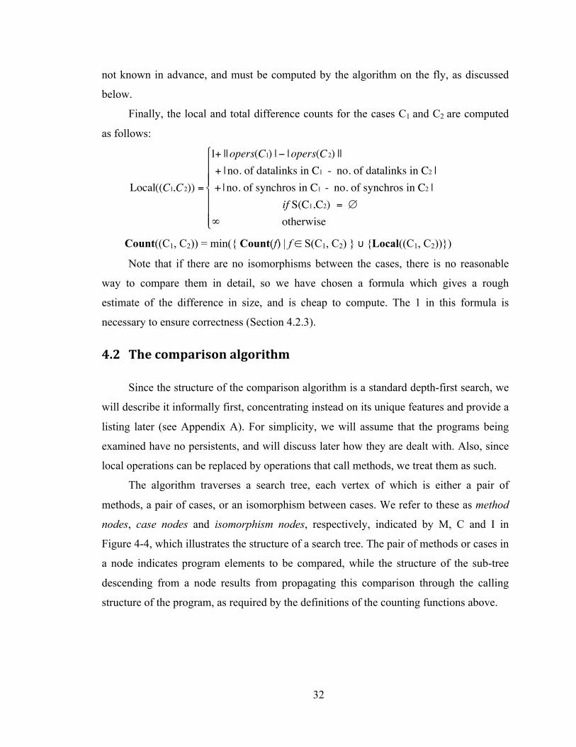
Finally, the local and total difference counts for the cases C1 and C2 are computed
as follows:
€
Local((C1,C2)) =
1+ ||opers(C1) | − |opers(C2) || + | no. of datalinks in C1 - no. of datalinks in C2 | + | no. of synchros in C1 - no. of synchros in C2 | if S(C1,C2) = ∅∞ otherwise
⎧
⎨
⎪ ⎪ ⎪
⎩
⎪ ⎪ ⎪
Count((C1, C2)) = min({ Count(f) | f ∈ S(C1, C2) } ∪ {Local((C1, C2))})
Note that if there are no isomorphisms between the cases, there is no reasonable
way to compare them in detail, so we have chosen a formula which gives a rough
estimate of the difference in size, and is cheap to compute. The 1 in this formula is
necessary to ensure correctness (Section 4.2.3).
4.2 The comparison algorithm
Since the structure of the comparison algorithm is a standard depth-first search, we
will describe it informally first, concentrating instead on its unique features and provide a
listing later (see Appendix A). For simplicity, we will assume that the programs being
examined have no persistents, and will discuss later how they are dealt with. Also, since
local operations can be replaced by operations that call methods, we treat them as such.
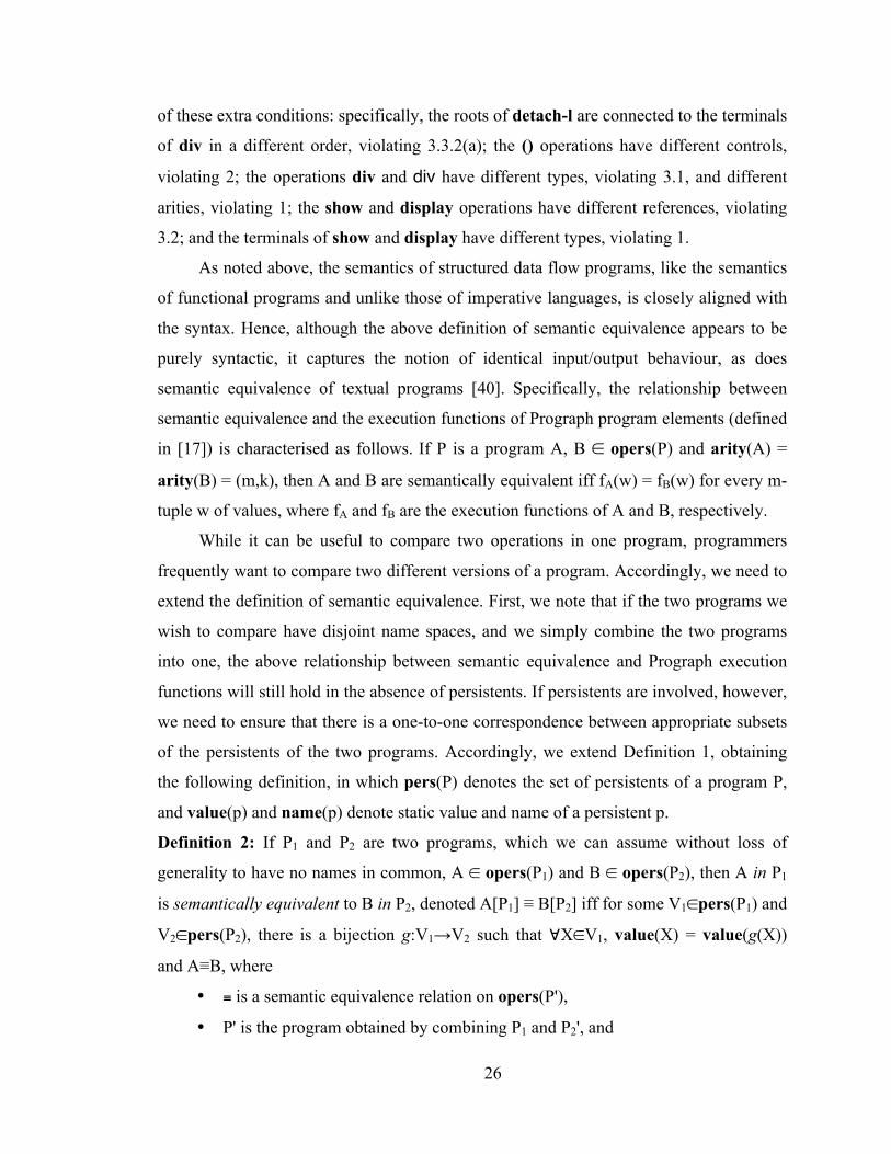
The algorithm traverses a search tree, each vertex of which is either a pair of
methods, a pair of cases, or an isomorphism between cases. We refer to these as method
nodes, case nodes and isomorphism nodes, respectively, indicated by M, C and I in
Figure 4-4, which illustrates the structure of a search tree. The pair of methods or cases in
a node indicates program elements to be compared, while the structure of the sub-tree
descending from a node results from propagating this comparison through the calling
structure of the program, as required by the definitions of the counting functions above.
33
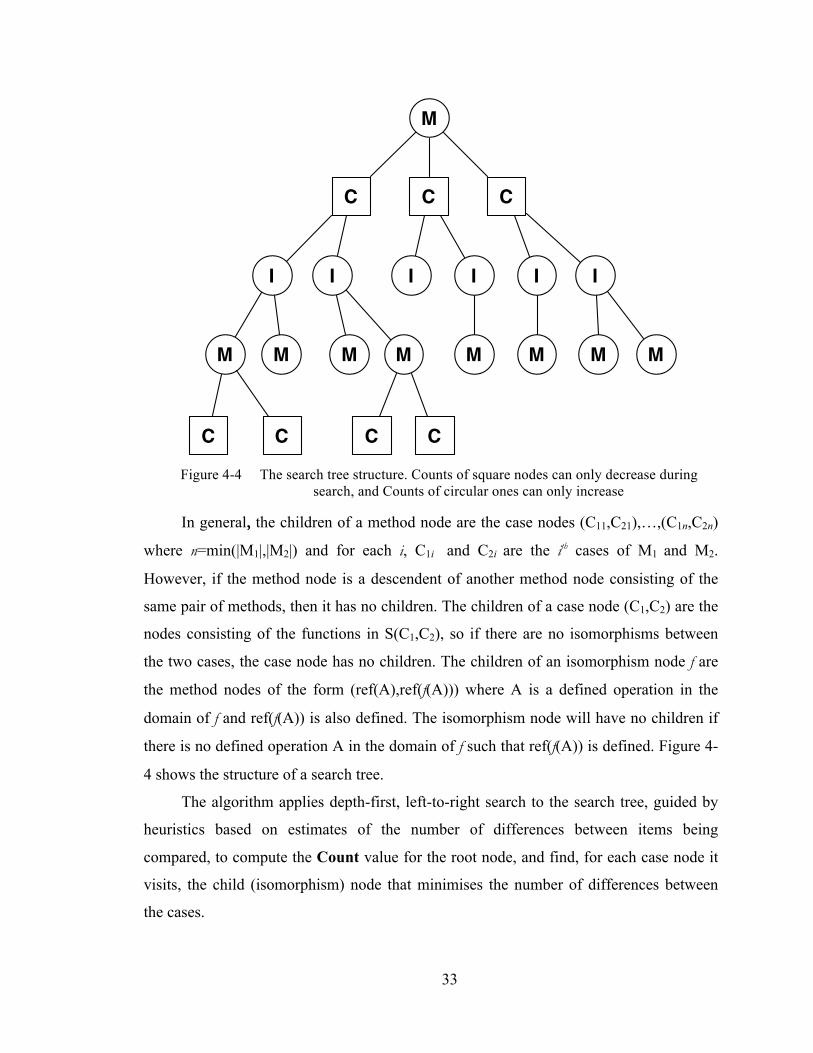
Figure 4-4 The search tree structure. Counts of square nodes can only decrease during
search, and Counts of circular ones can only increase
In general, the children of a method node are the case nodes (C11,C21),…,(C1n,C2n)
where n=min(|M1|,|M2|) and for each i, C1i and C2i are the ith cases of M1 and M2.
However, if the method node is a descendent of another method node consisting of the
same pair of methods, then it has no children. The children of a case node (C1,C2) are the
nodes consisting of the functions in S(C1,C2), so if there are no isomorphisms between
the two cases, the case node has no children. The children of an isomorphism node f are
the method nodes of the form (ref(A),ref(f(A))) where A is a defined operation in the
domain of f and ref(f(A)) is also defined. The isomorphism node will have no children if
there is no defined operation A in the domain of f such that ref(f(A)) is defined. Figure 4-
4 shows the structure of a search tree.
The algorithm applies depth-first, left-to-right search to the search tree, guided by
heuristics based on estimates of the number of differences between items being
compared, to compute the Count value for the root node, and find, for each case node it
visits, the child (isomorphism) node that minimises the number of differences between
the cases.
M
C
I I
C
I I I
M M M M M
C
I
M M M
C C CC
34
As search proceeds, the Count value for each node is incrementally computed as
the search tree below it is explored. The Count value of a case node is the minimum of
the Count values of its child nodes, while the Count value of each of the other nodes is
its Local value, plus the sum of the Counts of its children plus their local differences.
Hence the Counts of case nodes can only decrease during search while the Counts of
other nodes can only increase. We exploit this fact to reduce the number of nodes visited
by a technique similar to alpha-beta pruning [52].
When a node X is visited, three associated values are initialised, as follows.
As described below, these values change as the search proceeds in such a way that,
for each node X that is visited, the value of C(X) tends towards Count(X). As soon as
done(X) becomes true, further search in the subtree rooted at X is abandoned to avoid
exploring parts of the search tree that cannot affect the value of C that will be computed
for the root.
If node Y is the parent of a node X, and done(X) is assigned, or updated to, true,
then the values associated with Y are updated as follows.
if (Y is a method or isomorphism node)
1. then C(Y) = C(Y)+C(X)
2. else C(Y) = min(C(Y),C(X)) ;
if (done(Z) = true for every child Z of Y)
3. then done(Y) = true ;
if (Y is a case node and C(Y)=0)
4. then done(Y) = true ;
if (Y is a case node)
5. then alpha(Y) = min(alpha(Y),C(Y));
if (Y is a method or isomorphism node and C(Y) ≥ alpha(Y))
6. then done(Y) = true ;
35
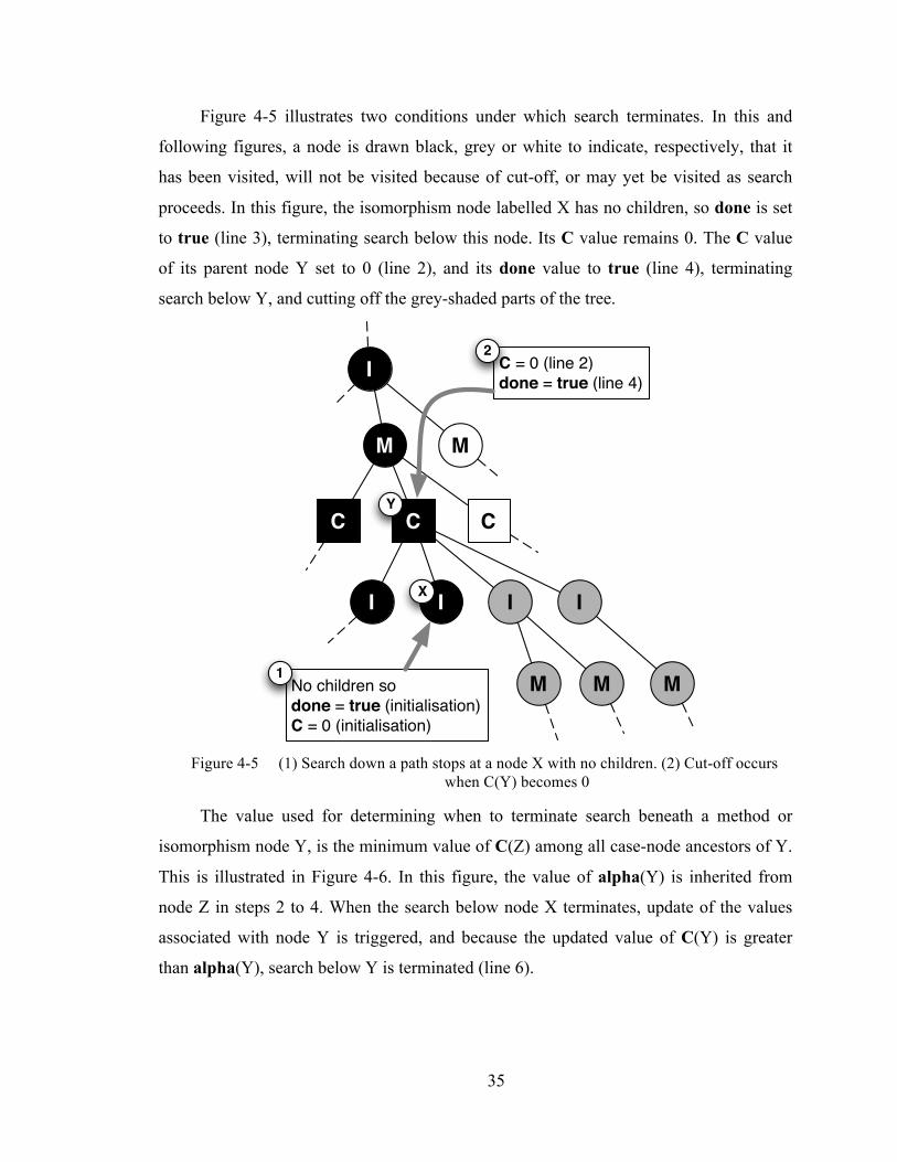
Figure 4-5 illustrates two conditions under which search terminates. In this and
following figures, a node is drawn black, grey or white to indicate, respectively, that it
has been visited, will not be visited because of cut-off, or may yet be visited as search
proceeds. In this figure, the isomorphism node labelled X has no children, so done is set
to true (line 3), terminating search below this node. Its C value remains 0. The C value
of its parent node Y set to 0 (line 2), and its done value to true (line 4), terminating
search below Y, and cutting off the grey-shaded parts of the tree.
Figure 4-5 (1) Search down a path stops at a node X with no children. (2) Cut-off occurs
when C(Y) becomes 0
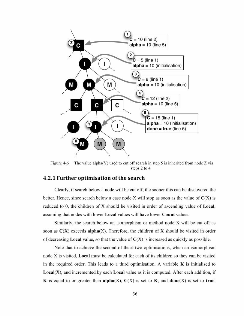
The value used for determining when to terminate search beneath a method or
isomorphism node Y, is the minimum value of C(Z) among all case-node ancestors of Y.
This is illustrated in Figure 4-6. In this figure, the value of alpha(Y) is inherited from
node Z in steps 2 to 4. When the search below node X terminates, update of the values
associated with node Y is triggered, and because the updated value of C(Y) is greater
than alpha(Y), search below Y is terminated (line 6).
M
C
I
C
I I I
M M M
I
No children sodone = true (initialisation)C = 0 (initialisation)
M
C
1
C = 0 (line 2)done = true (line 4)
2
X
Y
36
Figure 4-6 The value alpha(Y) used to cut off search in step 5 is inherited from node Z via
steps 2 to 4
4.2.1 Further optimisation of the search
Clearly, if search below a node will be cut off, the sooner this can be discovered the
better. Hence, since search below a case node X will stop as soon as the value of C(X) is
reduced to 0, the children of X should be visited in order of ascending value of Local,
assuming that nodes with lower Local values will have lower Count values.
Similarly, the search below an isomorphism or method node X will be cut off as
soon as C(X) exceeds alpha(X). Therefore, the children of X should be visited in order
of decreasing Local value, so that the value of C(X) is increased as quickly as possible.
Note that to achieve the second of these two optimisations, when an isomorphism
node X is visited, Local must be calculated for each of its children so they can be visited
in the required order. This leads to a third optimisation. A variable K is initialised to
Local(X), and incremented by each Local value as it is computed. After each addition, if
K is equal to or greater than alpha(X), C(X) is set to K, and done(X) is set to true,
M
C
I
C
I I
M
I
M
C
Y
M
CZ
M
I
X
C = 10 (line 2)alpha = 10 (line 5)
1
C = 5 (line 1)alpha = 10 (initialisation)
2
C = 8 (line 1)alpha = 10 (initialisation)
3
C = 12 (line 2)alpha = 10 (line 5)
4
C = 15 (line 1)alpha = 10 (initialisation)done = true (line 6)
5
M
37
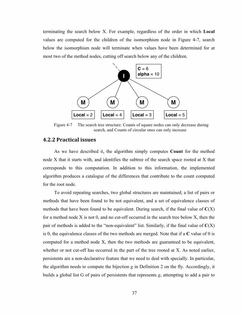
terminating the search below X. For example, regardless of the order in which Local
values are computed for the children of the isomorphism node in Figure 4-7, search
below the isomorphism node will terminate when values have been determined for at
most two of the method nodes, cutting off search below any of the children.
Figure 4-7 The search tree structure. Counts of square nodes can only decrease during
search, and Counts of circular ones can only increase
4.2.2 Practical issues
As we have described it, the algorithm simply computes Count for the method
node X that it starts with, and identifies the subtree of the search space rooted at X that
corresponds to this computation. In addition to this information, the implemented
algorithm produces a catalogue of the differences that contribute to the count computed
for the root node.
To avoid repeating searches, two global structures are maintained; a list of pairs or
methods that have been found to be not equivalent, and a set of equivalence classes of
methods that have been found to be equivalent. During search, if the final value of C(X)
for a method node X is not 0, and no cut-off occurred in the search tree below X, then the
pair of methods is added to the “non-equivalent” list. Similarly, if the final value of C(X)
is 0, the equivalence classes of the two methods are merged. Note that if a C value of 0 is
computed for a method node X, then the two methods are guaranteed to be equivalent,
whether or not cut-off has occurred in the part of the tree rooted at X. As noted earlier,
persistents are a non-declarative feature that we need to deal with specially. In particular,
the algorithm needs to compute the bijection g in Definition 2 on the fly. Accordingly, it
builds a global list G of pairs of persistents that represents g, attempting to add a pair to
I
M M M M
Local = 2 Local = 4 Local = 3 Local = 5
C = 6alpha = 10
38
this list when it encounters two operations, A and B, that are matched by an isomorphism,
but refer to two different persistents. There are three possibilities.
• If (ref(A),ref(B)) is in G, then A and B are considered to be equivalent.
• If (ref(A),P) is in G and P ≠ ref(B) (or vice versa), then A and B are considered
not to be equivalent.
• If neither ref(A) nor ref(B) occurs in any pair in G, (ref(A),ref(B)) is added to
G.
There is a complication, however. If the isomorphism f that matches A and B turns
out not to be the one which minimises the value of C(Y), where Y is the parent node of
the isomorphism node X corresponding to f, then the addition of (ref(A),ref(B)) to G must
be undone. Hence, when a pair is added to G, it is added provisionally, creating a local
list G(X), the scope of which is the search of the sub-tree rooted at X. When the final
value of C(Y) is determined, G is updated to G(Z), where Z is the selected child of Y.
4.2.3 Correctness and performance
If two programs are not equivalent, there is no precise answer to the question of
how they differ semantically [40], so there is little that can be proved about the
correctness of an algorithm such as ours with respect to semantic difference. However, it
does have an important property, as follows. If A and B are operations and P1 and P2, are
programs, the algorithm described above, including the optimisations in Section 4.2.1,
will compute a value of 0 for (ref(A),ref(B)) iff A in P1 is equivalent to B in P2 (Def. 2).
Although the subgraph isomorphism problem, central to our algorithm, is known to
be NP-complete, there are various subgraph isomorphism algorithms available which, in
practice, perform well on large graphs, for example Ullmann’s algorithm [53], VF [54],
and VF2 [55]. Also, Prograph programs tend to have a deep call structure, so even in a
large Prograph program, the number of operations in each case is usually quite small
[56]. For example, in the application framework of Prograph CPX, consisting of 2000+
methods distributed over 300+ classes, diagrams rarely have more than 6 operations.
Hence, subgraph isomorphism is unlikely to be a bottleneck.
39
As discussed in the last section, a set of equivalence classes of methods is
maintained to avoid repeating parts of a search. This set can be maintained by the
UNION-FIND algorithm in near-linear time [51].
Using subgraph isomorphism to match dataflow diagrams can in some
circumstances produce unsatisfactory results. For example, consider the pair (C1,C2) of
cases in Figure 4-8. These cases have the same numbers of operations, datalinks and
synchros, and there are no subgraph isomorphisms between them, so C((C1,C2)) will be
set to 1 and search below the case node (C1,C2) will terminate. Clearly, however, there
are two local differences (mismatched datalinks), and search should continue with the
method node (ref(A),ref(B)).
To solve this limitation, maximum common subgraph (MCS) isomorphism can be
used to find bijections between two graphs when subgraph isomorphism fails. There are
various definitions and algorithms for MCS in the research literature, such as McGregor
[47], Balas and Yu [57], and Durand et al. [58]. In this research, we choose the definition
of MCS implemented by McGregor’s algorithm, because the algorithm is easy to
implement and performs well. Suppose without loss of generality that graph G1 has fewer
vertices than graph G2.
if
• S1 is a subgraph of G1 including all vertices of G1
• S1 is isomorphic to a subgraph S2 of G2
• There is no subgraph of G1 with more edges than S1 satisfying these conditions
then
• S1 and S2 are corresponding maximum common subgraphs of G1 and G2.
Although the counting functions (described in section 4.1) are designed for use with
sub-graph isomorphism, they also apply to McGregor’s algorithm since all vertices in the
smaller graph will be included in the mapping. However, the time complexity of
McGregor’s algorithm in the worst case is factorial [56]. So we decided to implement
both sub-graph isomorphism and MCS isomorphism in the experiments to test their
effects on accuracy and performance.
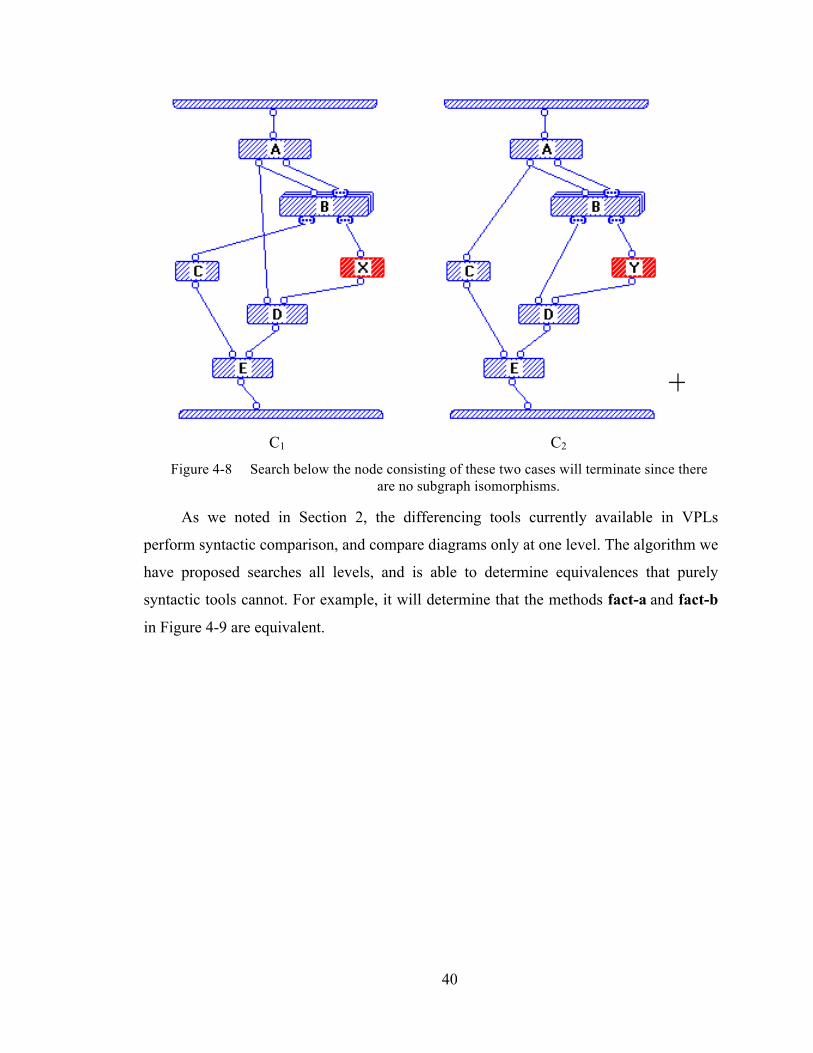
40
C1 C2
Figure 4-8 Search below the node consisting of these two cases will terminate since there are no subgraph isomorphisms.
As we noted in Section 2, the differencing tools currently available in VPLs
perform syntactic comparison, and compare diagrams only at one level. The algorithm we
have proposed searches all levels, and is able to determine equivalences that purely
syntactic tools cannot. For example, it will determine that the methods fact-a and fact-b
in Figure 4-9 are equivalent.
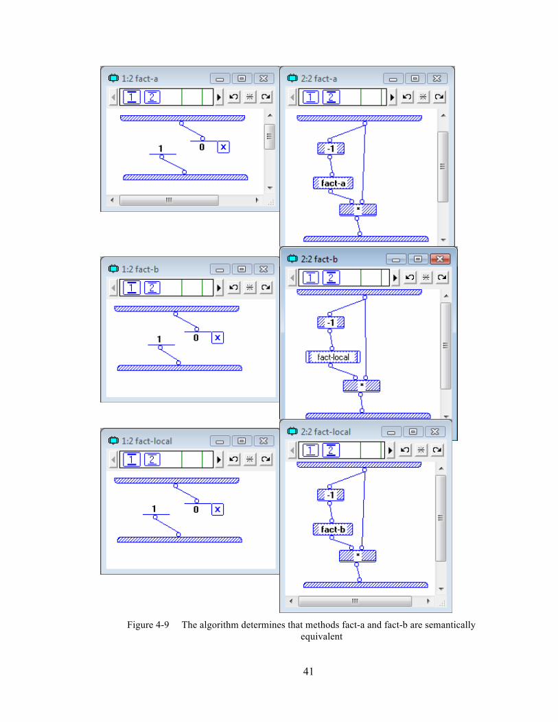
41
Figure 4-9 The algorithm determines that methods fact-a and fact-b are semantically
equivalent
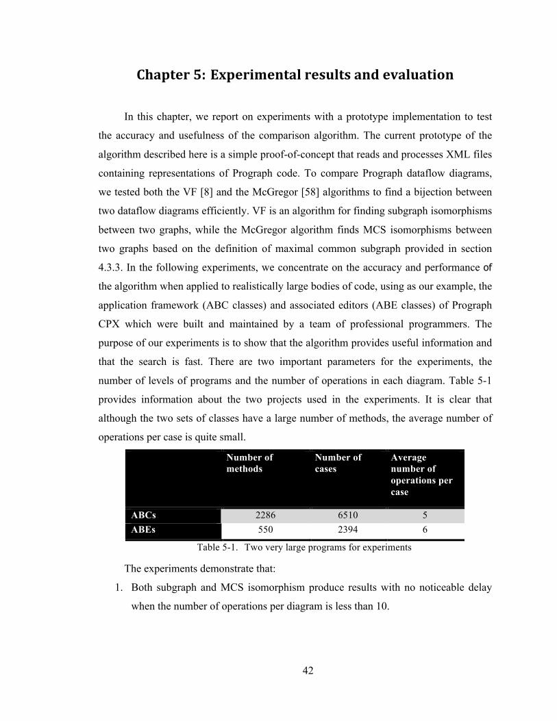
42
Chapter 5: Experimental results and evaluation
In this chapter, we report on experiments with a prototype implementation to test
the accuracy and usefulness of the comparison algorithm. The current prototype of the
algorithm described here is a simple proof-of-concept that reads and processes XML files
containing representations of Prograph code. To compare Prograph dataflow diagrams,
we tested both the VF [8] and the McGregor [58] algorithms to find a bijection between
two dataflow diagrams efficiently. VF is an algorithm for finding subgraph isomorphisms
between two graphs, while the McGregor algorithm finds MCS isomorphisms between
two graphs based on the definition of maximal common subgraph provided in section
4.3.3. In the following experiments, we concentrate on the accuracy and performance of
the algorithm when applied to realistically large bodies of code, using as our example, the
application framework (ABC classes) and associated editors (ABE classes) of Prograph
CPX which were built and maintained by a team of professional programmers. The
purpose of our experiments is to show that the algorithm provides useful information and
that the search is fast. There are two important parameters for the experiments, the
number of levels of programs and the number of operations in each diagram. Table 5-1
provides information about the two projects used in the experiments. It is clear that
although the two sets of classes have a large number of methods, the average number of
operations per case is quite small.
Number of methods
Number of cases
Average number of operations per case
ABCs 2286 6510 5 ABEs 550 2394 6
Table 5-1. Two very large programs for experiments
The experiments demonstrate that:
1. Both subgraph and MCS isomorphism produce results with no noticeable delay
when the number of operations per diagram is less than 10.
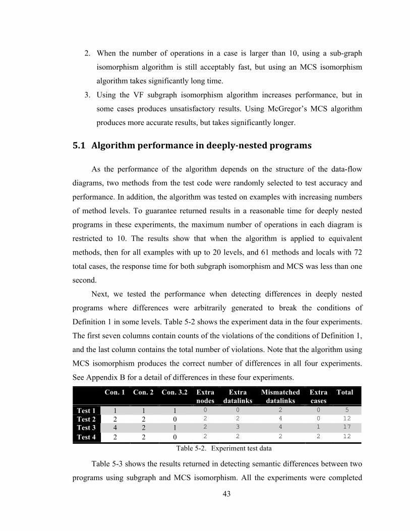
43
2. When the number of operations in a case is larger than 10, using a sub-graph
isomorphism algorithm is still acceptably fast, but using an MCS isomorphism
algorithm takes significantly long time.
3. Using the VF subgraph isomorphism algorithm increases performance, but in
some cases produces unsatisfactory results. Using McGregor’s MCS algorithm
produces more accurate results, but takes significantly longer.
5.1 Algorithm performance in deeply-nested programs
As the performance of the algorithm depends on the structure of the data-flow
diagrams, two methods from the test code were randomly selected to test accuracy and
performance. In addition, the algorithm was tested on examples with increasing numbers
of method levels. To guarantee returned results in a reasonable time for deeply nested
programs in these experiments, the maximum number of operations in each diagram is
restricted to 10. The results show that when the algorithm is applied to equivalent
methods, then for all examples with up to 20 levels, and 61 methods and locals with 72
total cases, the response time for both subgraph isomorphism and MCS was less than one
second.
Next, we tested the performance when detecting differences in deeply nested
programs where differences were arbitrarily generated to break the conditions of
Definition 1 in some levels. Table 5-2 shows the experiment data in the four experiments.
The first seven columns contain counts of the violations of the conditions of Definition 1,
and the last column contains the total number of violations. Note that the algorithm using
MCS isomorphism produces the correct number of differences in all four experiments.
See Appendix B for a detail of differences in these four experiments.
Con. 1 Con. 2 Con. 3.2 Extra nodes
Extra datalinks
Mismatched datalinks
Extra cases
Total
Test 1 1 1 1 0 0 2 0 5
Test 2 2 2 0 2 2 4 0 12
Test 3 4 2 1 2 3 4 1 17
Test 4 2 2 0 2 2 2 2 12
Table 5-2. Experiment test data
Table 5-3 shows the results returned in detecting semantic differences between two
programs using subgraph and MCS isomorphism. All the experiments were completed
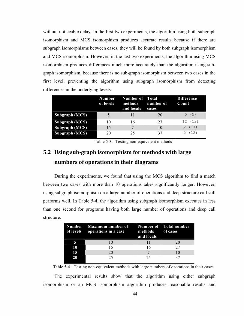
44
without noticeable delay. In the first two experiments, the algorithm using both subgraph
isomorphism and MCS isomorphism produces accurate results because if there are
subgraph isomorphisms between cases, they will be found by both subgraph isomorphism
and MCS isomorphism. However, in the last two experiments, the algorithm using MCS
isomorphism produces differences much more accurately than the algorithm using sub-
graph isomorphism, because there is no sub-graph isomorphism between two cases in the
first level, preventing the algorithm using subgraph isomorphism from detecting
differences in the underlying levels.
Number of levels
Number of methods and locals
Total number of cases
Difference Count
Subgraph (MCS) 5 11 20 5 (5)
Subgraph (MCS) 10 16 27 12 (12) Subgraph (MCS) 15 7 10 2 (17) Subgraph (MCS) 20 25 37 5 (12)
Table 5-3. Testing non-equivalent methods
5.2 Using sub-graph isomorphism for methods with large
numbers of operations in their diagrams
During the experiments, we found that using the MCS algorithm to find a match
between two cases with more than 10 operations takes significantly longer. However,
using subgraph isomorphism on a large number of operations and deep structure call still
performs well. In Table 5-4, the algorithm using subgraph isomorphism executes in less
than one second for programs having both large number of operations and deep call
structure.
Number of levels
Maximum number of operations in a case
Number of methods and locals
Total number of cases
5 10 11 20 10 15 16 27 15 20 7 10 20 25 25 37
Table 5-4. Testing non-equivalent methods with large numbers of operations in their cases
The experimental results show that the algorithm using either subgraph
isomorphism or an MCS isomorphism algorithm produces reasonable results and

45
performance in programs with small numbers of operations. However, the algorithm
using sub-graph isomorphism algorithm scales up with the number of operations in each
diagram considerably better than the algorithm using the MCS algorithm.
46
Chapter 6: Conclusions and future research
6.1 Conclusions
In this work, we have summarized and analyzed existing differencing tools for both
TPLs and DVPLs. In TPLs, syntactic and semantic differencing tools have been
intensively researched for use in software development tools since the introduction of
PDGs, SDGs, and program slicing. On the other hand, we found that differencing tools in
DVPLs are quite primitive compared with those available for TPLs. This in itself is
sufficient to hinder the successful entrance of DVPLs into the world of industrial
software development and mainstream software engineering.
Based on an investigation of the three differencing tools in DVPLs, as discussed
above, we concluded that they are all syntactic and therefore cannot find important
differences in many cases. Consequently, we have proposed a definition of semantic
equivalence of program elements in SVPLs and presented an algorithm to detect semantic
differences between SVPL program elements. To compare two dataflow diagrams, each
is considered as a directed acyclic graph and sub-graph isomorphism or MCS
isomorphism algorithms are applied to detect the differences between them. The problem
of comparing two program elements was modelled as a search tree, each vertex of which
is a pair of compared items or an isomorphism. Our differencing algorithm uses depth-
first search, guided by heuristics based on estimates of the numbers of differences
between the items being compared, to traverse the search tree and enumerate semantic
differences. Some of important features of the algorithm deal with recursions and side-
effects of persistents (global variables) and apply semantic equivalence and pruning
conditions to reduce the search space. The experimental results show that our algorithm
can produce the differences accurately in a reasonable time in most cases. When the
number of operations per case of programs is less than 10, the algorithm using both sub-
graph isomorphism and MCS isomorphism produces reasonably accurate results and a
reasonable time. When the number of operations per case of programs is larger, however,
the algorithm using subgraph isomorphism still performs reasonably, while the
performance using MCS rapidly degrades. Also, the algorithm using MCS isomorphism
47
can produce results more accurately in many cases. So MCS isomorphism can be used to
find a match between two graphs when sub-graph isomorphism fails. In conclusion, our
algorithm is superior to existing differencing tools for DVPLs.
6.2 Future work
There are many directions for furthering this work, including the following.
Object-oriented support: Our current algorithm does not account for the object-
oriented features of Prograph. Some features of object-oriented programming, such as
data abstraction, encapsulation, polymorphism, and inheritance, need to be dealt
differently with the current algorithm, for example, considering object-oriented
operations in Prograph as a global variable and treating them similar to the way of
treating persistents in the current algorithm. In the future, we can extend our algorithm to
define semantic equivalence on object-oriented classes in SVPLs.
Diagram matching: As we have pointed out, subgraph isomorphism can, in many
circumstances, produce results that are not helpful. Although MCS produces satisfactory
results, it does not scale up well as the number of operations per case increases. We
intend to investigate more discriminating ways of matching dataflow diagrams, such as a
variation that is sensitive to some dataflow-specific characteristics. For example, in
Prograph, we could build from a diagram a directed graph such that every operation,
terminal and root is represented as a vertex, the root and terminal vertices are numbered
to indicate the position at which the corresponding terminal or root is attached to its
operation, and an edge either represents a datalink or associates a terminal or root with its
operation. This graph would capture the structure of a Prograph case more accurately
than the graph used in the current version of the algorithm. Other graph matching
techniques, such as using genetic programming or approximation algorithms can also be
used.
Graphical interface: In Prograph, and other SVPLs, programming, testing and
debugging is done in highly interactive, visual environments that include visualisations of
execution state and progress. Clearly, an SVPL differencing tool should integrate into
such an environment, providing a visual representation, at various levels of detail, of the
trouble spots where differences are found, and helping the user to navigate through the
48
program structure in a methodical way. For example, two programs might be displayed as
two trees (similar to the LabVIEW comparison tool), with differences highlighted. First,
users could see the overall picture for the differences between two programs and know
the total number of differences. After that, they could select which differences they want
to fix. Since fixing errors in one level can reduce errors in many other levels, the tool
could guide programmers to a level where fixing differences would be likely to reduce
the number of steps for program testing and debugging. An incremental version of the
algorithm with a graphical interface would be developed in the future.
Pilot evaluation study for professional developers: After developing a graphical
interface for the algorithm, more user testing should be conducted with professional
software developers to find out whether a differencing tool based on our algorithm might
actually be of use to programmers in practice.
Counting function: Although the counting functions we have used to guide the
heuristic search seem to do a reasonable job on the examples we have tried, they can
produce misleading results. We intend to conduct a series of experiments on large
programs to pinpoint their weaknesses in order to fine-tune them.
Extending to other DVPLs: In this thesis, we have used Prograph as the language
on which to base our algorithm. However, with minor changes the algorithm could be
applied to other SVPLs, such as LabVIEW, where control structures enclose acyclic data
flow diagrams, consisting of operations with input terminals and output roots connected
by data flow links, and annotations can be applied to program elements to modify their
behaviours. More major changes are likely to be necessary in order to apply the algorithm
to unstructured DVPLs such as Simulink, where data flow diagram may be cyclic.
Other applications: Semantic difference is very important for software
development tools, such as program integration, program debugging, software
maintenance, and software testing. We can use this semantic differencing algorithm for
the purpose of program integration. For example, a merge tool integrates two versions of
an SVPL program by identifying the semantic differences and the un-affected code.
Detecting semantic changed behaviour will help to integrate two versions of a program
more accurately. Semantic difference is also useful to reduce the cost of regression

49
testing by discovering the semantic changes to decrease the number of test cases. These
tools would be very useful for accelerating the industrial adoption of SVPLs.
50
Bibliography
[1] R. E. Horn, Visual Language: Global Communication for the 21st Century.
MacroVU, Inc. Bain bridge Island, WA, 1998.
[2] P. T. Cox, “Visual Programming Languages,” Encyclopedia of Computer Science
and Engineering, B.W. Wah (Ed.) John Wiley & Sons Inc., Hoboken, Jun. 2008.
[3] M. Burnett, “Software Engineering For Visual Programming Languages,”
Handbook of Software Engineering and Knowledge, vol. 2, World Scientific
Publishing Company, Jun. 2001.
[4] Visual Case - UML & E/R Database Design Tool. Internet:
http://www.visualcase.com/ [Jul. 23, 2009].
[5] EJB and Java™ UML visual editing. Internet:
http://publib.boulder.ibm.com/infocenter/wsadhelp/v5r1m2/index.jsp?topic=/com
.rational.xtools.umlvisualizer.doc/topics/rlimitations.html [Jul. 23, 2009].
[6] Visual Paradigm SDE for Visual Studio. Internet:
http://www.visual-paradigm.com/product/sde/vs/demos/ [Jul. 23, 2009].
[7] R. Mili and R. Steiner, “Software Engineering,” in Software Visualization.
Springer Berlin / Heidelberg, 2002, ch. 2, pp. 622-624.
[8] IBM. Jinsight 2.1. Internet: http://www.research.ibm.com/jinsight/docs/ [Jul. 23,
2009].
[9] GraphViz. Internet: http://www.graphviz.org/ [Jul. 23, 2009].
[10] J. T. Stasko, J. T. Stasko, J. T. Stasko, and B. A. Price, Software visualization.
The MIT Press, Jan. 1998.
[11] S. Diehl, Software visualization: Visualizing the Structure, Behaviour, and
Evolution of Software. New York: Springer Berlin Heidelberg, 1998.
[12] StackAnalyzer. Internet: http://www.absint.com/stackanalyzer/ [Jul. 23, 2009].
[13] X-Tango: Algorithm Animation. Internet:
http://www.cc.gatech.edu/gvu/softviz/algoanim/xtango.html [Jul. 23, 2009].
51
Line Oriented Software Statistics,” IEEE Transactions on Software Engineering,
vol. 18, no. 11, pp. 957-968, Nov. 1992.
[15] B. A. Myers, “Visual programming, programming by example, and program
visualization: a taxonomy,” in Proceedings of the SIGCHI conference on Human
factors in computing systems, Boston, Massachusetts, United States , 1986, pp.
59-66.
[16] R. Bitter, T. Mohiuddin, and M. Nawrocki, LabVIEW: Advanced Programming
Techniques, 2e. CRC Press, 2001.
[17] Prograph CPX User guide, Halifax, Canada: Pictorius Inc., 1996.
[18] M. M. Burnett, “Visual Programming,”, Wiley Encyclopedia of Electrical and
Electronics Engineering, J. Webster (ed.), John Wiley&Sons Inc., pp. 275-283,
1999.
[19] Microsoft Visual C++. Internet: http://msdn.microsoft.com/en-
ca/visualc/default.aspx [Jul. 23, 2009].
[20] Microsoft Visual J++. Internet: http://msdn.microsoft.com/en-
us/vjsharp/default.aspx [Jul. 23, 2009].
[21] Prograph CPX Reference Manual. Halifax: Pictorius Inc., 1996.
[22] Simulink. Internet: http://www.mathworks.com/products/simulink/ [Jul. 23,
2009].
[23] R. B. Angus and T. E. Hulbert, “VEE Pro: Practical Graphical Programming,”
Springer-Verlag, London, 2005.
[24] P. T. Cox, F.R. Giles, and Pietrzykowski T., “Prograph: a step towards liberating
programming from textual conditioning,” in 1989 IEEE Workshop on Visual
Programming, Rome, Oct. 1989, pp. 150-156.
[25] W. M. Johnston, J. R. P. Hanna, and R. J. Millar, “Advances in dataflow
programming languages,” ACM Computing Surveys (CSUR), vol. 36, no. 1, pp.
1-34, Mar. 2004.
[26] S. T. Karris, Introduction to Simulink with Engineering Applications, 2e,. Orchard
52
Publications, 2008.
[27] A. F. Blackwell, “First steps in programming: A rationale for Attention
Investment models,” in Proceedings of the IEEE Symposia on Human-Centric
Computing Languages and Environments, Washington DC, Sep. 2002, pp. 2-10.
[28] R. Rowe and J. Burns, Prograph CPX Qualitative Research. Riley Rowe and
Associates, 1995.
[29] P. T. Cox and L. Dong, “Obstacles to the industrial use of visual programming,”
in 2004 International Conference on Visual Languages and Computing, San
Francisco CA, Sep. 2004, pp. 304-311.
[30] P. T. Cox and S. Gauvin, “Exceptions in Visual Data Flow Programming
Languages,” in 2003 International Conference on Visual Languages and
Computing, Miami FL, Sep. 2003, pp. 360-367.
[31] J. Vesperman, Essential CVS, 2e. Sebastopol CA: O’Reilly Media Inc., 2007.
[32] B. Collins-Sussman, B. W. Fitzpatrick, and C. M. Pilato, Version Control with
Subversion. Sebastopol CA: O'Reilly Media Inc., 2004.
[33] J. W. Hunt and M. D. McIlroy, “An algorithm for differential file comparison,”
Technical Memo 75-1271-11, Bell Laboratories, Oct. 1975.
[34] W. Miller and E. W. Myers, “A file comparison program,”, Software Practice &
Experience, vol. 15, no. 11, pp. 1025-1040, Nov. 1985.
[35] E. W. Myers, “An O(ND) difference algorithm and its variations,”, Algorithmica,
vol. 1, no. 2, p. 251–266, 1986.
[36] E. Ukkonen, “Algorithms for Approximate String Matching,” Information and
Control, vol. 64, no. 1-3, pp. 100-118, 1985.
[37] W. Yang, “Identifying Syntactic Differences Between Two Programs,” Software
Practice And Experience, vol. 21, no. 7, pp. 739-755, Jul. 1991.
[38] J. E. Grass, “Cdiff: A Syntax Directed Diff for C++ Programs,” in USENlX C++
Conference, Portland, 1992, pp. 181-193.
[39] D. Binkley, “An empirical study of the effect of semantic differences on
53
programmer comprehension,” in 10th International Workshop on Program
Comprehension (IWPC'02), Paris, France, Jun. 2002, pp. 97-106.
[40] D. Jackson and D. A. Ladd, “Semantic Diff: A tool for summarizing the effects of
modifications,” in Proceedings of the International Conference on Software
Maintenance, Victoria, BC, Canada, 1994, pp. 243-252.
[41] P. Anderson and T. Teitelbaum, “Software inspection using codesurfer,” in
Workshop on Inspection in Software Engineering, 2001.
[42] S. Horwitz, “Identifying the semantic and textual differences between two
versions of a program,”, ACM SIGPLAN Notices, vol. 25, no. 6, pp. 234-245, Jun.
1990.
[43] F. Tip, “A Survey of Program Slicing Techniques,” CWI (Centre for Mathematics
and Computer Science) , Amsterdam, The Netherlands, The Netherlands,
Technical Report CS-R9438 , 1994.
[44] B. Xu, J. Qian, X. Zhang, Z. Wu, and L. Chen, “A Brief Survey Of Program
Slicing,” A Brief Survey Of Program Slicing, vol. 30, no. 2, p. 1, Mar. 2005.
[45] S. Horwitz, J. Prins, and T. Reps, “Integrating non-interfering versions of
programs,”, ACM Transactions on Programming Languages and Systems, vol.
13, no. 3, pp. 345-387, Jul. 1989.
[46] W. Yang, S. Horwitz, and T. Reps, “Detecting program components with
equivalent behaviors,” Department of Computer Sciences, University of
Wisconsin, Madison, WI, Technical Report 840, Apr. 1989.
[47] J. McGregor, “Backtrack search algorithms and the maximal common subgraph
problem,” Software Practice and Experience, vol. 12, pp. 23-34, 1982.
[48] D. Binkley, S. Horwitz, and T. Reps, “Program Integration for Languages with
Procedure Calls,” ACM Transactions on Software Engineering and Methodology
(TOSEM), vol. 4, no. 1, pp. 3-35, Jan. 1995.
[49] D. Binkley, “Semantics guided regression test cost reduction,” IEEE Transactions
on Software Engineering, vol. 23, no. 8, pp. 498-516, Aug. 1997.
54
[51] R. E. Tarjan, “Efficiency of a Good But Not Linear Set Union Algorithm,”,
Journal of the ACM, vol. 22, no. 2, pp. 215-225, Apr. 1975.
[52] G.M. Baudet, “An analysis of the full alpha-beta pruning algorithm,” in
Proceedings of the tenth annual ACM Smposium on Theory of Computing, 1978,
pp. 296-313.
[53] J. R. Ullmann, “An Algorithm for Subgraph Isomorphism,” Journal of the ACM,
vol. 23, no. 1, pp. 31-42, Jan. 1976.
[54] L. P. Cordella, P. Foggia, C. Sansone, and M. Vento, “Performance evaluation of
the VF graph matching algorithm,” in Proceedings of the 10th International
Conference on Image Analysis, Venice, Italy, 1999, pp. 1172-1177.
[55] L. P. Cordella, P. Foggia, C. Sansone, and M. Vento, “An Improved Algorithm
for Matching Large Graphs,” in 3rd IAPRTC15 Workshop on Graph-based
Representations in Pattern Recognition, Cuen, Italy, 2001, pp. 149-159.
[56]
T. R. G. Green and M. Petre, “Usability analysis of visual programming
environments: a ‘cognitive dimensions’ framework,” Journal of Visual
Languages and Computing, vol. 7, no. 2, pp. 131-174, Jun. 1996.
[57] E. Balas and C. S. Yu, “Finding a maximum clique in an arbitrary graph,” SIAM J. Computing, vol. 15, no.4, 1986.
[58]
P. J. Durand, R. Pasari, J. W. Baker, and C. Tsai, “An efficient algorithm for similarity analysis of molecules,” Internet Journal of Chemistry, vol. 2, 1999.
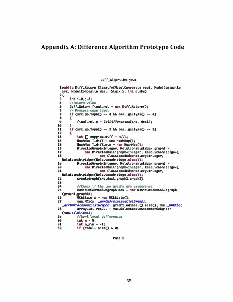
55
Appendix A: Difference Algorithm Prototype Code
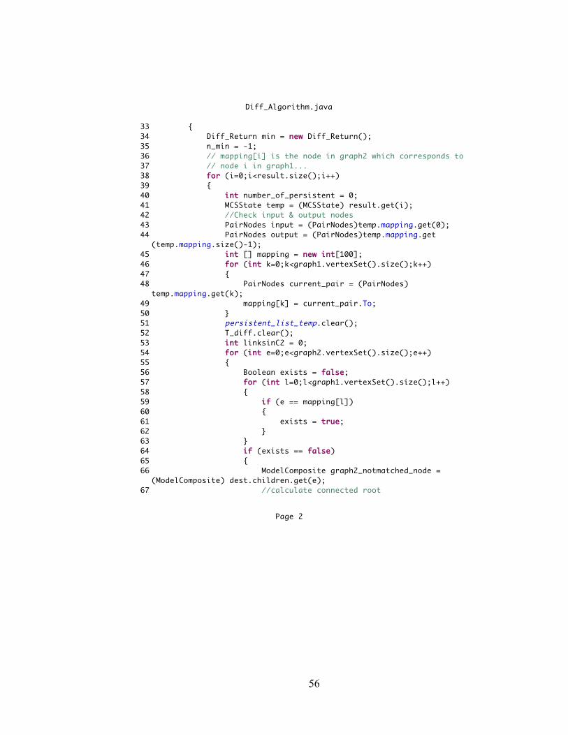
56
Diff_Algorithm.java
33 {34 Diff_Return min = new Diff_Return();35 n_min = -1;36 // mapping[i] is the node in graph2 which corresponds to37 // node i in graph1...38 for (i=0;i<result.size();i++)39 {40 int number_of_persistent = 0; 41 MCSState temp = (MCSState) result.get(i);42 //Check input & output nodes43 PairNodes input = (PairNodes)temp.mapping.get(0);44 PairNodes output = (PairNodes)temp.mapping.get
(temp.mapping.size()-1);45 int [] mapping = new int[100];46 for (int k=0;k<graph1.vertexSet().size();k++)47 {48 PairNodes current_pair = (PairNodes)
temp.mapping.get(k);49 mapping[k] = current_pair.To; 50 }51 persistent_list_temp.clear();52 T_diff.clear();53 int linksinC2 = 0;54 for (int e=0;e<graph2.vertexSet().size();e++)55 {56 Boolean exists = false;57 for (int l=0;l<graph1.vertexSet().size();l++)58 {59 if (e == mapping[l])60 {61 exists = true;62 }63 }64 if (exists == false)65 {66 ModelComposite graph2_notmatched_node =
(ModelComposite) dest.children.get(e);67 //calculate connected root
Page 2
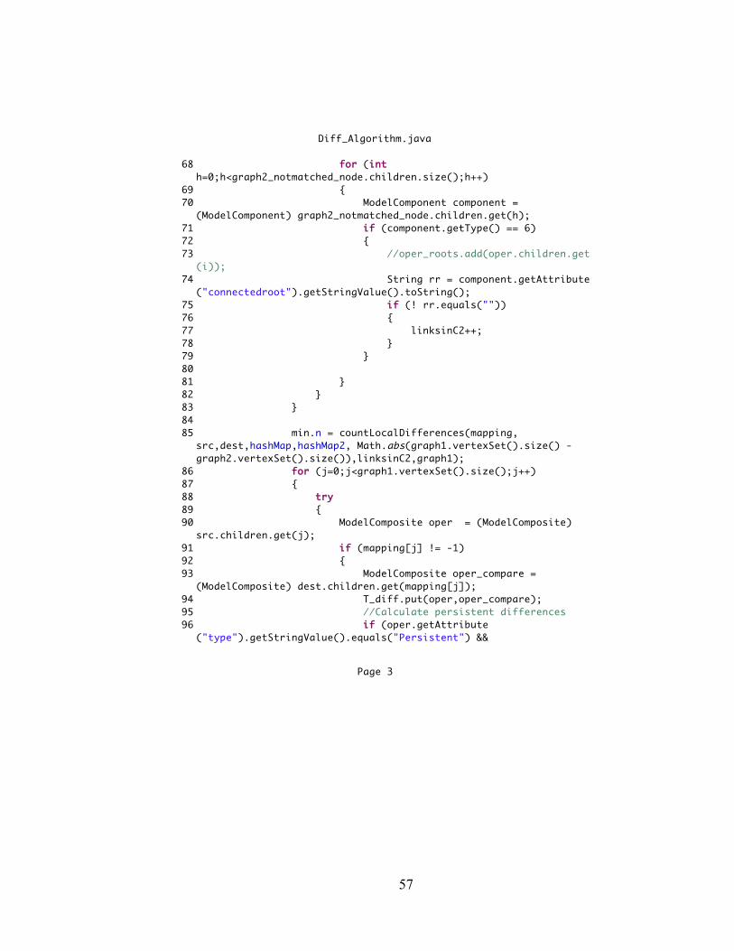
57
Diff_Algorithm.java
68 for (int h=0;h<graph2_notmatched_node.children.size();h++)
69 {70 ModelComponent component =
(ModelComponent) graph2_notmatched_node.children.get(h);71 if (component.getType() == 6)72 {73 //oper_roots.add(oper.children.get
(i));74 String rr = component.getAttribute
("connectedroot").getStringValue().toString();75 if (! rr.equals(""))76 {77 linksinC2++;78 }79 }80 81 }82 }83 }84 85 min.n = countLocalDifferences(mapping,
src,dest,hashMap,hashMap2, Math.abs(graph1.vertexSet().size() - graph2.vertexSet().size()),linksinC2,graph1);
86 for (j=0;j<graph1.vertexSet().size();j++)87 {88 try89 {90 ModelComposite oper = (ModelComposite)
src.children.get(j); 91 if (mapping[j] != -1)92 {93 ModelComposite oper_compare =
(ModelComposite) dest.children.get(mapping[j]);94 T_diff.put(oper,oper_compare);95 //Calculate persistent differences96 if (oper.getAttribute
("type").getStringValue().equals("Persistent") && oper_compare.getAttribute("type").getStringValue().equals("Persistent")) Page 3

58
Diff_Algorithm.java96 if (oper.getAttribute("type").getStringValue().equals("Persistent") && oper_compare.getAttribute("type").getStringValue().equals("Persistent"))
97 {98 Boolean p_ret = isConsistent
(oper,oper_compare); 99 if (p_ret == true)
100 {101 number_of_persistent++;102 Equivalent_List per = new
Equivalent_List();103 per.src = oper;104 per.dest = oper_compare;105 persistent_list.add(per);106 }107 else108 {109 min.n ++;110 }111 }112 if (min.n >= alpha)113 {114 final_ret.n = alpha;115 F_T_list list = new F_T_list
(graph1.vertexSet().size());116 list.f = mapping;117 list.T = T_diff;118 final_ret.f_T.add(list);119 return final_ret;120 }121 122 if (oper.getAttribute
("type").getStringValue().equals("method") && oper_compare.getAttribute("type").getStringValue().equals("method"))
123 {124 125 ModelComposite method_1 = null;126 ModelComposite method_2 = null;127 method_1 = (ModelComposite)
hashMap.get(oper.getName());
Page 4
59
Diff_Algorithm.java127 method_1 = (ModelComposite)
hashMap.get(oper.getName());128 129 method_2 = (ModelComposite)
hashMap2.get(oper_compare.getName());130 Boolean ret = isProcessing
(method_1, method_2);131 if (ret == false)132 {133 Diff_Return ret1 = Classify
(root, method_1, method_2, S,alpha);134 min.n += ret1.n;135 min.f_T.add(ret1.f_T);136 if (min.n >= alpha)137 {138 final_ret.n = alpha;139 F_T_list list = new F_T_list
(graph1.vertexSet().size());140 list.f = mapping;141 list.T = T_diff;142 final_ret.f_T.add(list);143 return final_ret;144 }145 }146 }147 }148 }149 catch (Exception ex)150 {151 152 }153 154 }155 156 if (n_min == -1 || min.n < n_min)157 {158 n_min = min.n;159 mapping_diff = mapping;160 T_diff_min = T_diff;
Page 5
60
Diff_Algorithm.java
161 }162 163 if (min.n == 0)164 {165 n_min = min.n;166 mapping_diff = mapping;167 T_diff_min = T_diff;168 break;169 }170 171 }172 //Return case value173 final_ret.n = n_min;174 F_T_list list = new F_T_list(graph1.vertexSet().size());175 list.f = mapping_diff;176 list.T = T_diff_min;177 final_ret.f_T.add(list);178 return final_ret;179 }180 else181 {182 Diff_Return ret = new Diff_Return();183 ret.n = 1 + Math.abs(graph1.vertexSet().size() -
graph2.vertexSet().size()) + Math.abs(graph1.edgeSet().size()-graph2.edgeSet().size());
184 return ret;185 }186 }187 else188 {189 }190 //Process method level. Use HashMap for methods' call191 if ((src.getType() == 2 && dest.getType() == 2) || (src.getType
() == 20 && dest.getType() == 20))192 {193 //Check if method already exists in the list S194 Boolean ret = isProcessing(src, dest);195 if (ret == true)
Page 6
61
Diff_Algorithm.java
196 {197 return final_ret;198 }199 else200 {201 Equivalent_List method = new Equivalent_List();202 method.src = src;203 method.dest = dest;204 processing_oper.push(method);205 }206 //Check if method already exists in the list E207 ret = isEquivalent(src, dest);208 if (ret == true)209 {210 return final_ret;211 }212 //Check if method already exists in the list N213 Equivalent_List e_list = new Equivalent_List();214 e_list = isNotEquivalent(src, dest);215 if (e_list.n != 0)216 {217 final_ret.n = e_list.n;218 final_ret.f_T = e_list.f_T;219 return final_ret;220 }221 //Loop each case222 //Extra cases223 final_ret.n += Math.abs(src.children.size() -
dest.children.size());224 if (final_ret.n >= alpha)225 {226 //Cut-off 3227 }228 else229 {230 for (i = 0;i < src.children.size();i++)231 {232 ModelComposite m_case = (ModelComposite)
src.children.get(i);
Page 7
62
Diff_Algorithm.java232 ModelComposite m_case = (ModelComposite)
src.children.get(i);233 ModelComposite m_case_comp = (ModelComposite)
dest.children.get(i);234 //Add up all the differences235 Diff_Return c_ret = new Diff_Return();236 c_ret = Classify(root,m_case,m_case_comp,S,alpha);237 final_ret.n += c_ret.n;238 final_ret.f_T.add(c_ret.f_T);239 //cut-off240 if (final_ret.n >= alpha)241 {242 break;243 }244 }245 246 }247 //Remove from Stack248 processing_oper.pop();249 //Put in the equivalent list250 if (final_ret.n == 0)251 {252 Equivalent_List list = new Equivalent_List();253 list.dest = dest;254 list.src = src;255 equivalent_call_list.add(list);256 return final_ret;257 }258 else //put in the not-equivalent list (n,a,b,F)259 {260 Equivalent_List list = new Equivalent_List();261 list.dest = dest;262 list.src = src;263 list.n = final_ret.n;264 list.f_T.add(final_ret.f_T);265 nonequivalent_call_list.add(list);266 267 return final_ret;268 }
Page 8
63
Diff_Algorithm.java
269 }270 return null;271 }272 private int countLocalDifferences(int[] mapping, ModelComposite src,273 274 ModelComposite dest, HashMap hashMap, HashMap hashMap2, int
node_difference, int linkinC2, DirectedGraph g1) {275 276 // TODO Auto-generated method stub277 int n = 0,i,j;278 int n_min = -1;279 //Count local differences280 for (j=0;j<g1.vertexSet().size();j++)281 {282 try283 {284 ModelComposite oper = (ModelComposite) src.children.get
(j);285 if (mapping[j] != -1)286 {287 ModelComposite oper_compare = (ModelComposite)
dest.children.get(mapping[j]);288 n += GetDifferences(oper, oper_compare); //
Calculate operation differences289 }290 }291 catch (Exception ex)292 {293 }294 }295 ////CALCULATION LINKS IN C2 NOT IN C1296 n += linkinC2;297 int correct_datalinks=0;298 //Calculate mismatch data-links299 Set set = h_relation.entrySet();300 Iterator itr = set.iterator();301 while (itr.hasNext())302 {
Page 9
64
Diff_Algorithm.java
303 Map.Entry me = (Map.Entry)itr.next();304 ModelRelation current = (ModelRelation)me.getValue();305 ModelComponent from = current.from;306 ModelComponent to = current.to;307 ModelComposite m_from = (ModelComposite) from.getParent();308 ModelComposite m_to = (ModelComposite) to.getParent();309 String k = item_id.get(m_from.getID()).toString();310 String l = item_id.get(m_to.getID()).toString();311 if (mapping[Integer.parseInt(k)] != -1 && mapping
[Integer.parseInt(l)] != -1)312 {313 ModelComposite m_from_comp = (ModelComposite)
dest.children.get(mapping[Integer.parseInt(k)]);314 ModelComposite m_to_comp = (ModelComposite)
dest.children.get(mapping[Integer.parseInt(l)]);315 correct_datalinks += GetMismatchDatalinks(m_from, m_to,
m_from_comp, m_to_comp);316 }317 }318 //fINAL CALCULATION319 int num_of_terminals = 0;320 for (j=0;j< src.children.size();j++)321 {322 try323 {324 ModelComposite current = (ModelComposite)
src.children.get(j);325 for (int m=0;m<current.size();m++)326 {327 ModelComponent model = (ModelComponent)
current.children.get(m);328 if (model.getType() == 7)329 {330 num_of_terminals++;331 }332 }333 }334 catch(Exception ex)
Page 10
65
Diff_Algorithm.java
335 {336 }337 }338 n += num_of_terminals - correct_datalinks;339 //Calculate the number of nodes340 n += node_difference; 341 //Calculate persistent differences342 }343 private static int GetMismatchDatalinks(ModelComposite m_from,344 ModelComposite m_to, ModelComposite m_from_comp,345 ModelComposite m_to_comp) {346 // TODO Auto-generated method stub347 int n = 0,i,j;348 ArrayList oper_roots = new ArrayList();349 ArrayList oper_terms = new ArrayList();350 ArrayList oper_compare_roots = new ArrayList();351 ArrayList oper_compare_terms = new ArrayList();352 for (i=0;i<m_from.children.size();i++)353 {354 ModelComponent component = (ModelComponent)
m_from.children.get(i);355 if (component.getType() == 6)356 {357 oper_roots.add(m_from.children.get(i));358 }359 }360 for (i=0;i<m_to.children.size();i++)361 {362 ModelComponent component = (ModelComponent)
m_to.children.get(i);363 if (component.getType() == 7)364 {365 oper_terms.add(m_to.children.get(i));366 }367 }368 for (i=0;i<m_from_comp.children.size();i++)369 {370 ModelComponent component = (ModelComponent)
m_from_comp.children.get(i);
Page 11
66
Diff_Algorithm.java370 ModelComponent component = (ModelComponent)
m_from_comp.children.get(i);371 372 if (component.getType() == 6)373 {374 oper_compare_roots.add(m_from_comp.children.get(i));375 }376 }377 378 for (i=0;i<m_to_comp.children.size();i++)379 {380 ModelComponent component = (ModelComponent)
m_to_comp.children.get(i);381 if (component.getType() == 7)382 {383 oper_compare_terms.add(m_to_comp.children.get(i));384 }385 }386 387 if (oper_terms.size() == oper_compare_terms.size() &&
oper_roots.size() == oper_compare_roots.size())388 {389 //If( roots(a)j has datalink to terms(b)k for some j and k
and roots(f(a))j don�t have datalink terms(f(b))k)390 for (i=0;i<oper_terms.size();i++)391 {392 ModelComponent c_terms = (ModelComponent) oper_terms.get
(i);393 ModelComponent c_terms_comp = (ModelComponent)
oper_compare_terms.get(i);394 String root = c_terms.getAttribute
("connectedroot").getStringValue().toString();395 String root_compare = c_terms_comp.getAttribute
("connectedroot").getStringValue().toString();396 397 //First condition: Compare their roots equivalent398 for (j=0;j<oper_roots.size();j++)399 {400 ModelComponent c_root = (ModelComponent)
oper_roots.get(j);
Page 12
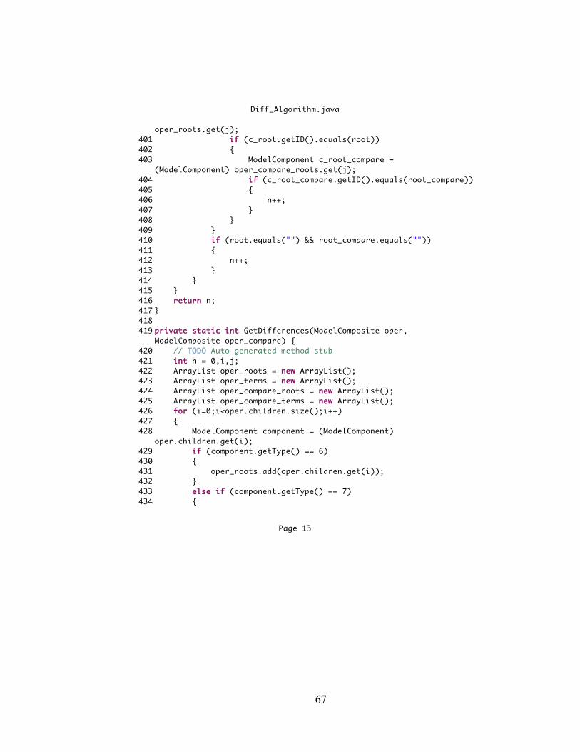
67
Diff_Algorithm.java400 ModelComponent c_root = (ModelComponent)
oper_roots.get(j);401 if (c_root.getID().equals(root))402 {403 ModelComponent c_root_compare =
(ModelComponent) oper_compare_roots.get(j);404 if (c_root_compare.getID().equals(root_compare))405 {406 n++;407 }408 }409 }410 if (root.equals("") && root_compare.equals(""))411 {412 n++;413 }414 }415 }416 return n;417 }418 419 private static int GetDifferences(ModelComposite oper,
ModelComposite oper_compare) {420 // TODO Auto-generated method stub421 int n = 0,i,j;422 ArrayList oper_roots = new ArrayList();423 ArrayList oper_terms = new ArrayList();424 ArrayList oper_compare_roots = new ArrayList();425 ArrayList oper_compare_terms = new ArrayList();426 for (i=0;i<oper.children.size();i++)427 {428 ModelComponent component = (ModelComponent)
oper.children.get(i);429 if (component.getType() == 6)430 {431 oper_roots.add(oper.children.get(i));432 }433 else if (component.getType() == 7)434 {
Page 13
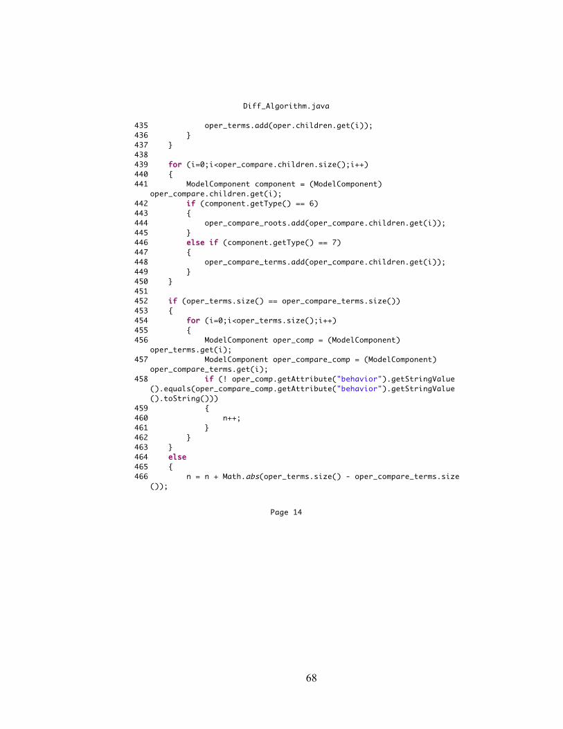
68
Diff_Algorithm.java
435 oper_terms.add(oper.children.get(i));436 }437 }438 439 for (i=0;i<oper_compare.children.size();i++)440 {441 ModelComponent component = (ModelComponent)
oper_compare.children.get(i);442 if (component.getType() == 6)443 {444 oper_compare_roots.add(oper_compare.children.get(i));445 }446 else if (component.getType() == 7)447 {448 oper_compare_terms.add(oper_compare.children.get(i));449 }450 }451 452 if (oper_terms.size() == oper_compare_terms.size())453 {454 for (i=0;i<oper_terms.size();i++)455 {456 ModelComponent oper_comp = (ModelComponent)
oper_terms.get(i);457 ModelComponent oper_compare_comp = (ModelComponent)
oper_compare_terms.get(i);458 if (! oper_comp.getAttribute("behavior").getStringValue
().equals(oper_compare_comp.getAttribute("behavior").getStringValue().toString()))
459 {460 n++;461 }462 }463 }464 else465 {466 n = n + Math.abs(oper_terms.size() - oper_compare_terms.size
());
Page 14
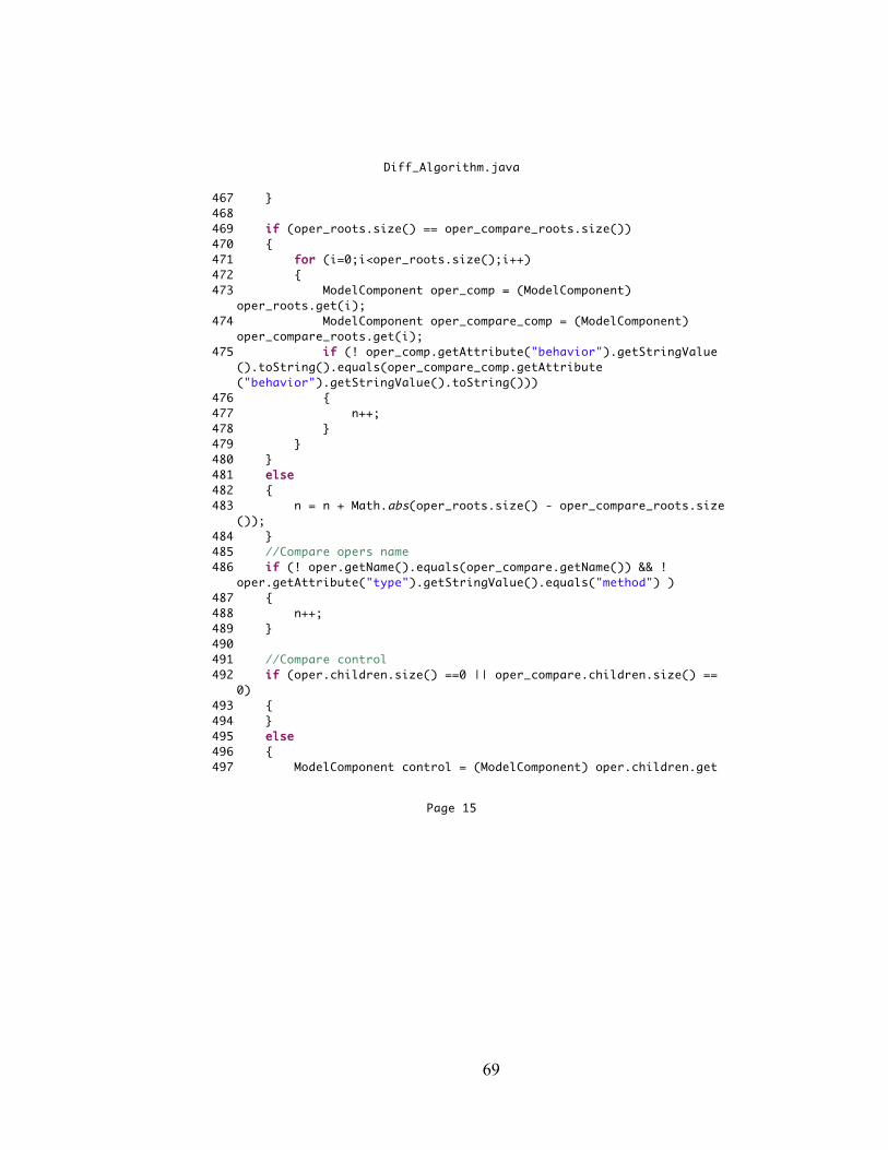
69
Diff_Algorithm.java
467 }468 469 if (oper_roots.size() == oper_compare_roots.size())470 {471 for (i=0;i<oper_roots.size();i++)472 {473 ModelComponent oper_comp = (ModelComponent)
oper_roots.get(i);474 ModelComponent oper_compare_comp = (ModelComponent)
oper_compare_roots.get(i);475 if (! oper_comp.getAttribute("behavior").getStringValue
().toString().equals(oper_compare_comp.getAttribute("behavior").getStringValue().toString()))
476 {477 n++;478 }479 }480 }481 else482 {483 n = n + Math.abs(oper_roots.size() - oper_compare_roots.size
());484 }485 //Compare opers name486 if (! oper.getName().equals(oper_compare.getName()) && !
oper.getAttribute("type").getStringValue().equals("method") )487 {488 n++;489 }490 491 //Compare control492 if (oper.children.size() ==0 || oper_compare.children.size() ==
0)493 {494 }495 else496 {497 ModelComponent control = (ModelComponent) oper.children.get
(0);
Page 15

70
Diff_Algorithm.java497 ModelComponent control = (ModelComponent) oper.children.get
(0);498 ModelComponent control_comp = (ModelComponent)
oper_compare.children.get(0);499 if (! control.getName().equals(control_comp.getName()))500 {501 n++;502 }503 }504 //Compare type505 if (oper.getType() == 0)506 {507 if (oper.getName().equals(oper_compare.getName()))508 {509 n++;510 }511 }512 return n;513 }514 515
Page 16
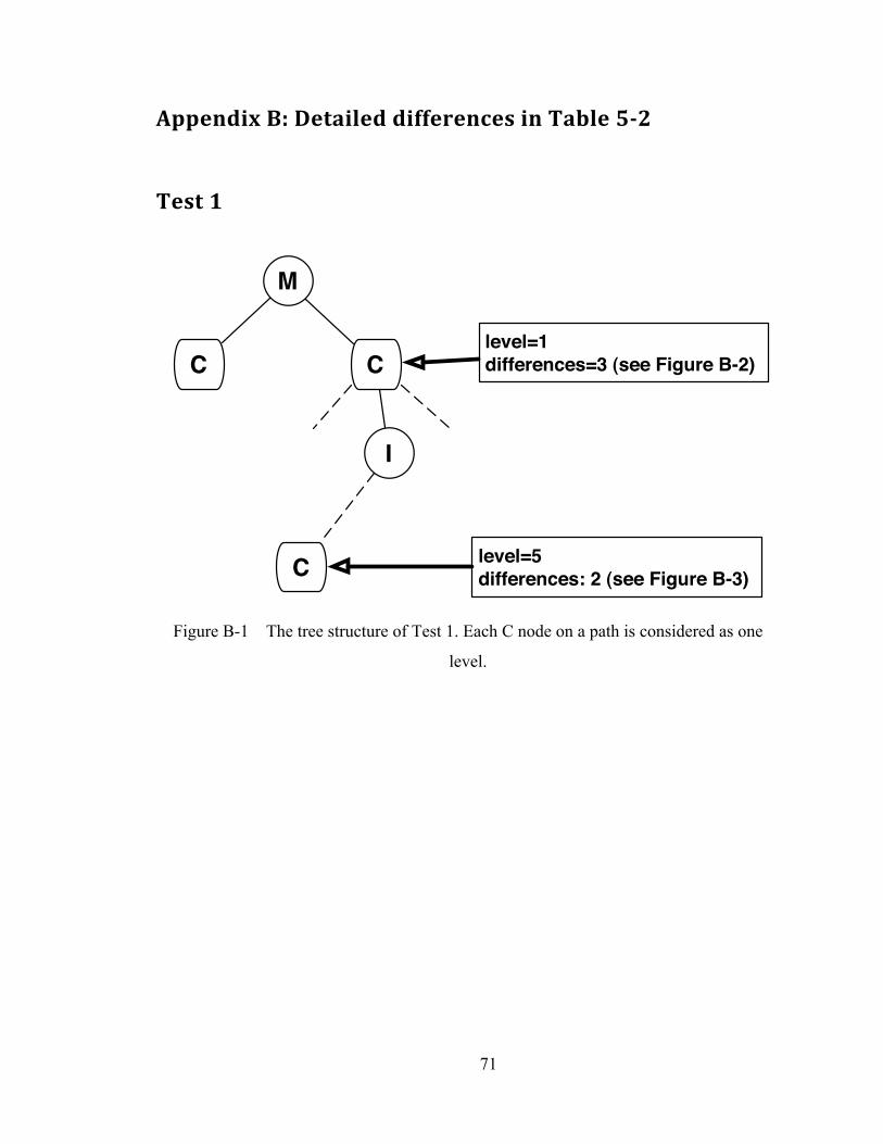
71
Appendix B: Detailed differences in Table 5-2
Test 1
Figure B-1 The tree structure of Test 1. Each C node on a path is considered as one
level.
I
CClevel=1differences=3 (see Figure B-2)
level=5differences: 2 (see Figure B-3)
M
C
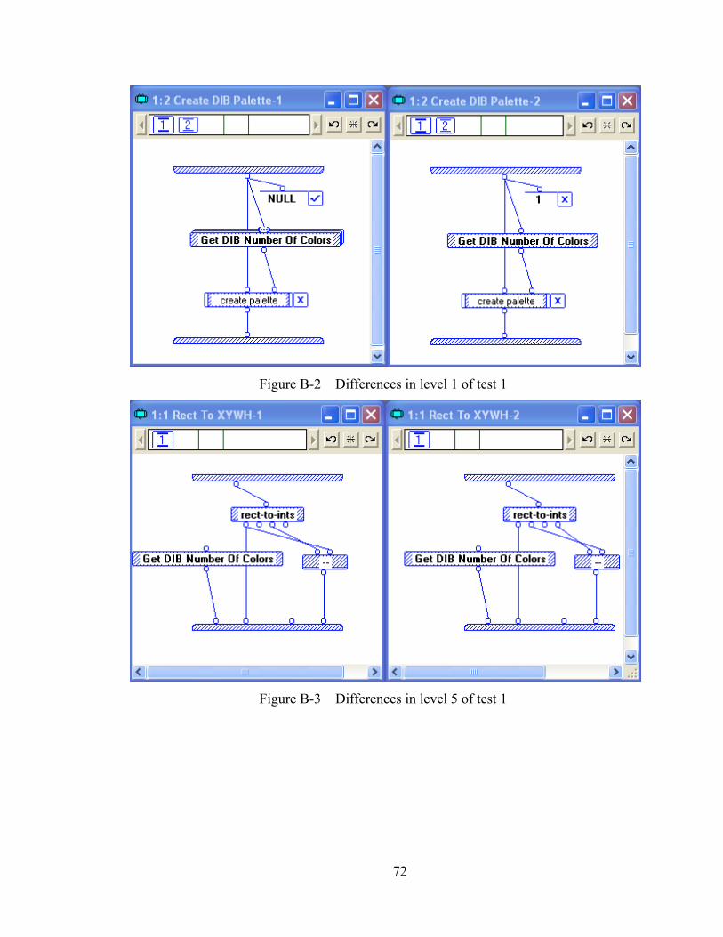
72
Figure B-2 Differences in level 1 of test 1
Figure B-3 Differences in level 5 of test 1
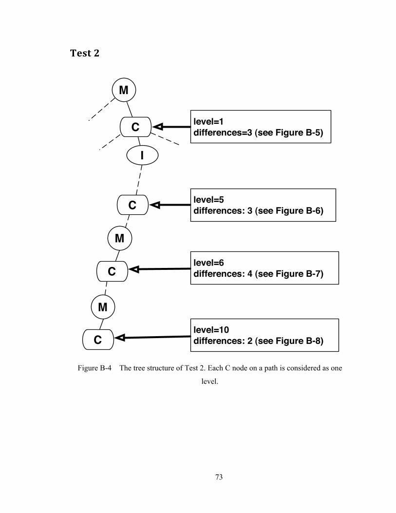
73
Test 2
Figure B-4 The tree structure of Test 2. Each C node on a path is considered as one
level.
I
C level=1differences=3 (see Figure B-5)
level=5differences: 3 (see Figure B-6)C
Clevel=6differences: 4 (see Figure B-7)
Clevel=10differences: 2 (see Figure B-8)
M
M
M

74
Figure B-5 Differences in level 1 of test 2
Figure B-6 Differences in level 5 of test 2

75
Figure B-7 Differences in level 6 of test 2
Figure B-8 Differences in level 10 of test 2
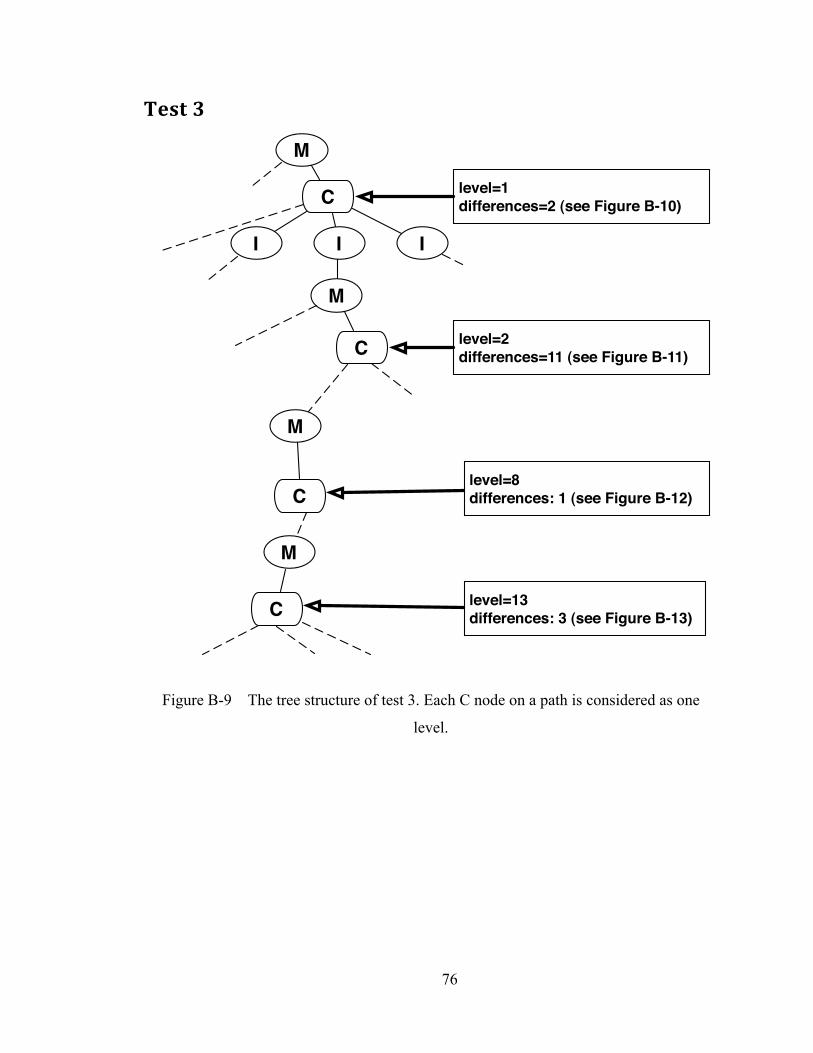
76
Test 3
Figure B-9 The tree structure of test 3. Each C node on a path is considered as one
level.
I I
C
I
M
C
level=1differences=2 (see Figure B-10)
Clevel=8differences: 1 (see Figure B-12)
C level=13differences: 3 (see Figure B-13)
level=2differences=11 (see Figure B-11)
M
M
M
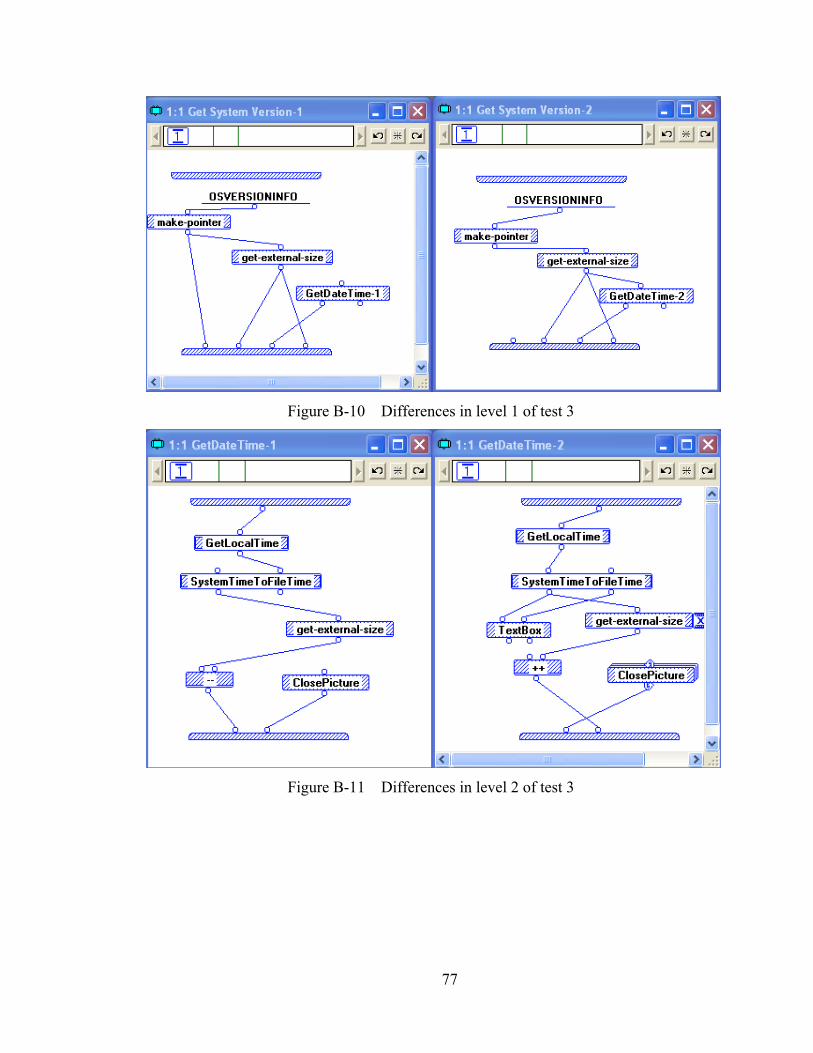
77
Figure B-10 Differences in level 1 of test 3
Figure B-11 Differences in level 2 of test 3

78
Figure B-12 Differences in level 8 of test 3
Figure B-13 Differences in level 13 of test 3
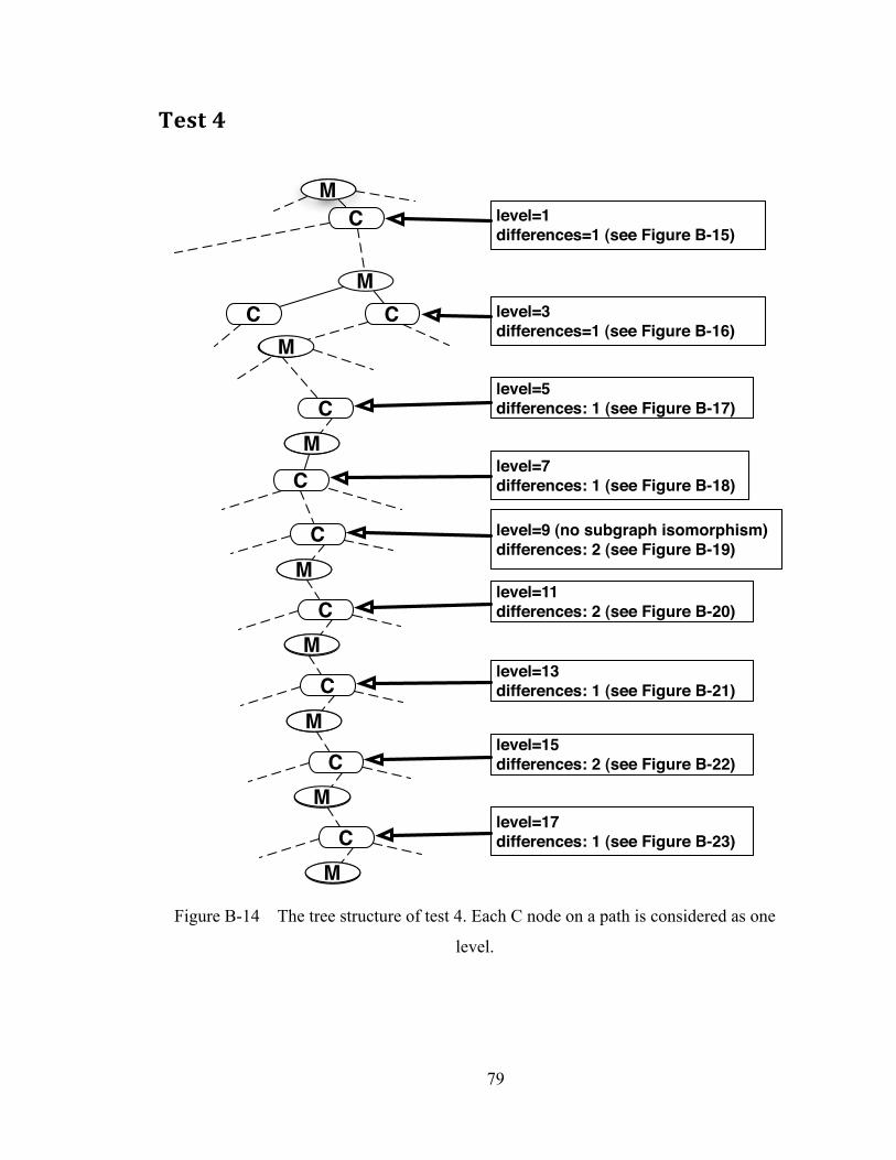
79
Test 4
Figure B-14 The tree structure of test 4. Each C node on a path is considered as one
level.
C
MCC
level=1differences=1 (see Figure B-15)
M
M
Clevel=5differences: 1 (see Figure B-17)
MC
level=7differences: 1 (see Figure B-18)
level=3differences=1 (see Figure B-16)
C level=9 (no subgraph isomorphism)differences: 2 (see Figure B-19)
M
Clevel=11differences: 2 (see Figure B-20)
M
Clevel=13differences: 1 (see Figure B-21)
M
Clevel=15differences: 2 (see Figure B-22)
M
Clevel=17differences: 1 (see Figure B-23)
M
M
M
M
M
M
M
M
M
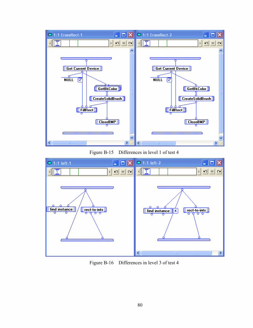
80
Figure B-15 Differences in level 1 of test 4
Figure B-16 Differences in level 3 of test 4
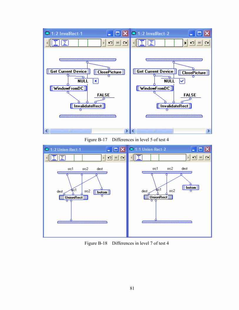
81
Figure B-17 Differences in level 5 of test 4
Figure B-18 Differences in level 7 of test 4

82
Figure B-19 Differences in level 9 of test 4 (no subgraph isomorphism)
Figure B-20 Differences in level 11 of test 4
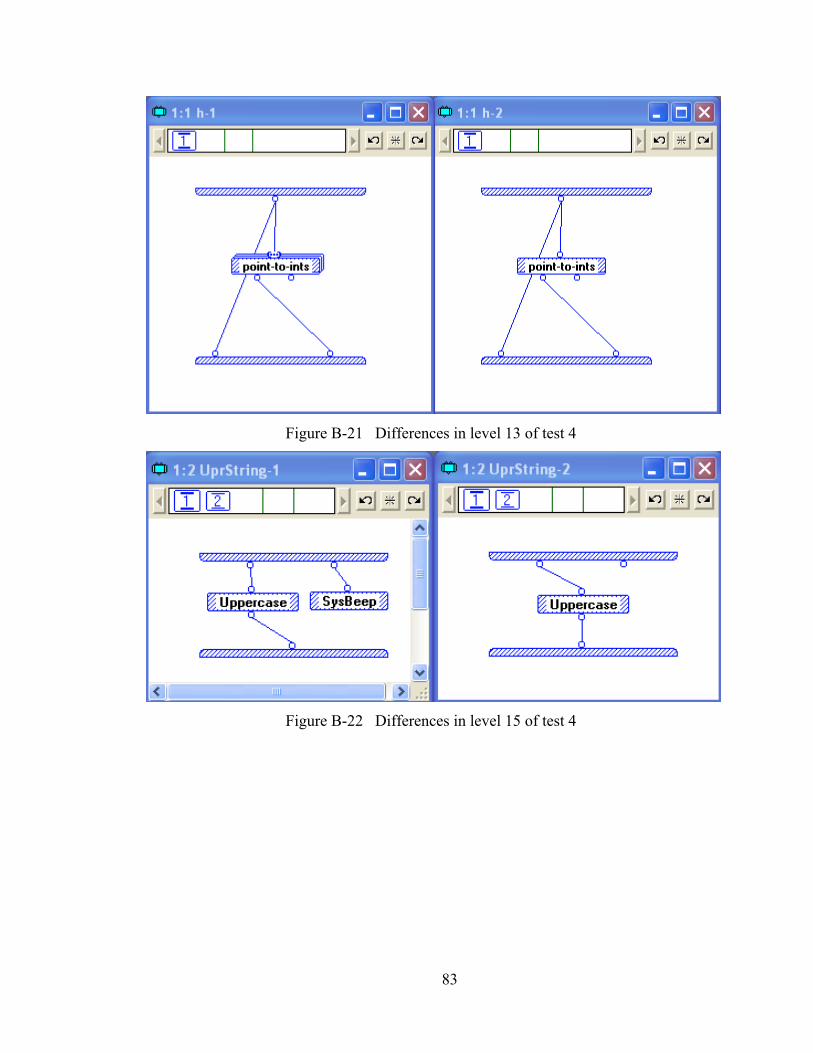
83
Figure B-21 Differences in level 13 of test 4
Figure B-22 Differences in level 15 of test 4
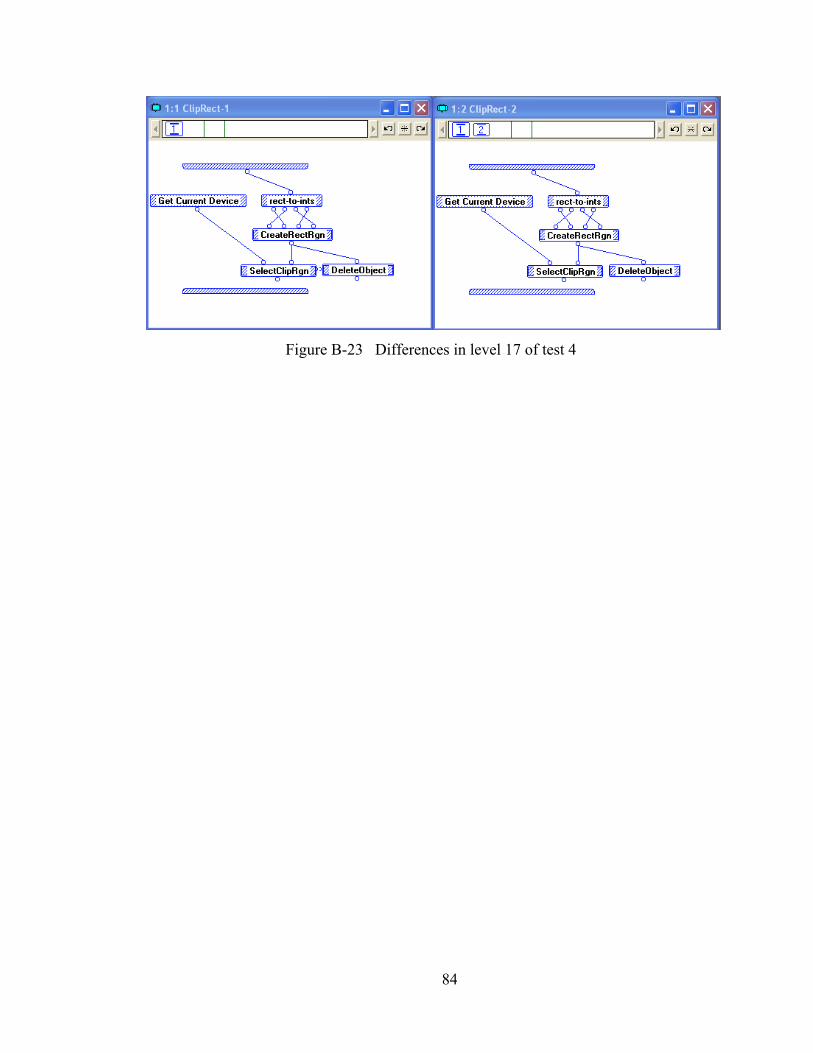
84
Figure B-23 Differences in level 17 of test 4