Selling to Heterogeneous Strategic Customers with UncertainValuations under Returns Policies

We consider a firm selling a fixed amount of inventory to customers who possess uncertain

valuations on a product prior to purchase and realize their complete valuations only after

purchase. The firm determines the returns policies over two periods; each of which targets

for a group of brand loyal customers or regular shoppers. The customers are strategic, taking

into account both the product availability risk and the product misfit risk when they decide

when to purchase. We identify two effects of returns including the positive effect of delay

mitigation and the negative effect of surplus reduction, resulting in no returns to brand

loyal customers in the first period and a positive refund to regular shoppers in the second

period. The result complements Su (2009)’s finding - returns itself is not beneficial for the

firm when faced with homogeneous customers with uncertain valuations. However, when

customers have distinct and uncertain valuations, returns offered in a later period mitigates

the incentive of loyal customers to delay their purchases. Hence, returns provides the firm

with an additional instrument to mitigate the negative consequences of strategic customer

behavior. We find that, with returns, the markup can emerge as the optimal pricing policy

when the firm holds a high inventory. We also investigate how the benefit of returns over no

returns is affected by the firm’s initial inventory level and customer valuation uncertainty.

1 Introduction

Dynamic pricing has become a common tool in the retailing industry to price discriminate

and extract higher revenues from customers with distinct product valuations. However, due

1

to the rapid growth of information technology, customers have become increasingly sophis-

ticated in their purchase decisions. For example, customers may strategize over the timing

of their purchases and are referred to as strategic customers. Obviously, their strategic pur-

chase behavior jeopardizes a firm’s profit. To counteract the adverse impact of strategic

purchase behavior, several useful approaches have been proposed and studied in the existing

literature. For example, a firm can ration inventory to create shortages at a low price to

induce early purchases from high-valuation customers at a high price (Liu and van Ryzin

2008). When a firm has a quick response capability, it can eliminate customers’ waiting in-

centive by reducing the chance of discounting the remaining inventory (Cachon and Swinney

2009). A seller may use an appropriate inventory display format, e.g., displaying one unit

of product, to create an increased sense of availability risk, and hence induce purchases at a

full price. A posterior price matching policy can discourage strategic delay behavior because

customers who have made early purchase are compensated for price difference if the price is

marked down later on (Lai, Debo, and Sycara 2010).

One assumption that is commonly made in this stream of literature is that customers

precisely know their own valuations on the product. However, in many real-world examples,

customers often do not know their exact valuations on the product when they make purchase

decisions. Such valuation uncertainty may arise in a number of ways. For example, when

customers purchase an innovative or highly fashionable product, they are not sure about their

exact values because they have not experienced such a product before. When customers buy

products (such as clothing, shoes) via an online channel, the shipped products may not fit

for sizes, styles, or their expectations.

Faced with a group of customers who privately possess some initial yet incomplete val-

uations about the product before purchase and realize the complete valuations only after

purchase, a firm can offer returns which allows the customers to return products and get

refunds. Hence, a returns policy essentially provides customers with an insurance that al-

leviates their concerns about the ex ante uncertainty of product value. As a result, returns

encourages more purchases from customers whose valuations are less certain. On the other

hand, returns is costly for the firm since it has to pay a refund for the returned product. Can

2

a firm then benefit from an appropriately designed returns policy? Su (2009) answers this

question by revealing that the cost of refund outweighs the benefit of demand enhancement

and hence returns itself is not a useful tool to generate more profits from homogeneous cus-

tomers who share the same mean value on the product. Does the result hold when customers

have distinct and uncertain valuations? This is the main question to be address in the paper.

The focus of our work is to investigate the role of returns in coping with strategic purchase

behavior when customers possess heterogeneous and uncertain valuations.

We consider a stylized model in which a firm sells a fixed amount of inventory to a

heterogeneous market with two segments of customers: the brand loyal customers and the

regular shoppers. All customers are ex ante uncertain about the product value, and brand

loyal customers value the product more than regular shoppers in the sense of first-order

dominance. To price discriminate the two customer segments, the firm offers two distinct

returns policies in sequel, each of which targets a specific customer segment. Each selling

policy consists of a selling price and a returns refund. All the customers are strategic and

present at the beginning of the selling horizon. They decide to purchase either now or

later. Due to limited supply, customers who delay purchases may not obtain the product.

Hence, taking shortage risk into account, strategic customers compare expected surpluses

of purchasing the product under different returns policies offered in different periods, and

choose the one that maximizes their expected surplus. We characterize the firm’s optimal

returns policies, and obtain the following main findings.

First, with regard to the question of whether or not offering returns is useful for the

firm, we find that the firm should not offer returns to brand loyal customers in the first

period, and that the firm should offer positive returns refund to regular shoppers in the

second period. The former result of zero refund to the loyal customers is consistent with

Su (2009)’s finding, following the insight that returns is ineffective in profit extraction. The

latter result that a positive refund is offered to the regular shoppers reveals the strategic role

of returns in weakening customers’ strategic waiting behavior. Specifically, a loyal customer

values a refund less than a regular shopper because she is less likely to return the product.

Consequently, relative to zero refund, a positive refund allows the firm to charge a higher

3

selling price in the second period so that it is still appealing to the regular shoppers but

less so for the loyal customers, thereby reducing the loyal customers’ incentive to wait. In

determining the optimal refund level in the second period, the firm needs to balance the

tradeoff between the positive effect of weakening the loyal customers’ strategic waiting and

the negative effect of extracting less profits from the regular shoppers.

Second, we find that the returns might reverse the order of the two prices offered in two

periods. Without returns, it is well known that the firm’s optimal pricing policy takes the

form of markdown. In contrast, with returns, we find that the markup pricing is optimal when

returns offered to regular shoppers in the second period is sufficiently generous, a scenario

that occurs when there is a stronger need to diminish the incentive of strategic delay behavior

of brand loyal customers. For example, for a sufficiently large amount of inventory, a threat

of “sold out” is minimal and hence loyal customers have a strong incentive to delay purchase.

Therefore, a generous refund is required to thwart the purchase delay of loyal customers so

that the selling price in the second period may exceed the first-period selling price.

Third, we identify and explore two drivers that influence the benefits from using returns

relative to no returns for the firm. The first driver is the inventory level. We show that

the firm gains more profits under returns compared with no returns as the inventory level

increases. The intuition is that a higher inventory level reduces the shortage risk and thus

intensifies the loyal customers’ delay purchase incentive, and hence there is a stronger need

for the firm to offer distinct returns refunds to counteract such waiting behavior. The second

driver is the customers’ ex ante uncertainty. Contrary to the conventional wisdom that the

firm benefits from a reduction in customer valuation uncertainty, we show that the firm is

worse off when the customer valuation uncertainty is smaller.

2 Literature Review

This paper is closely related to the stream of papers on strategic customer behavior in the

operations management literature, especially those focusing on strategic waiting behavior

and its impact on a firm’s pricing and inventory decisions. Strategic waiting behavior weak-

4

ens a firm’s ability to use intertemporal price discrimination to extract more surpluses from

customers. This result has been revealed by Aviv and Pazgal (2008), Zhang and Cooper

(2008), and Cachon and Swinney (2009), to name a few. To counteract such an adverse

consequence of strategic waiting behavior, several mechanisms and approaches are investi-

gated under a variety of selling strategies. For example, Aviv and Pazgal (2008) examine the

effectiveness of two classes of pricing strategies - inventory-contingent markdown and pre-

announced fixed discount - in dealing with strategic waiting behavior. Liu and van Ryzin

(2008) show that capacity rationing can be effectively used to mitigate the negative effect

of strategic customer behavior because a shortage risk created by rationing induces early

purchases at a higher price. Yin et al. (2009) find that a firm’s in-store display format can

influence customers’ perception of availability risk and thus their decision on buying now

or later. They find that an appropriately designed display format such as display one unit

is generally useful to discourage strategic customers from waiting for price discount. Lai,

Debo and Sycara (2010) establish that a posterior price matching policy can eliminate the

waiting incentive of strategic customers and it is therefore especially effective for a market

with a large number of strategic customers whose valuations decline moderately over time.

Cachon and Swinney (2009) reveal that a quick response empowering the firm an ability to

better match supply and demand leads to a low level of clearance sales, and hence reduces

the delay incentive of strategic customers. Li and Zhang (2013) investigate the pre-order,

a strategy used to obtain advance demand information so that improve product availability

in the regular selling season. Because an increased product availability enhances the delay

incentive of strategic customers, the value of the pre-order strategy is reduced in the presence

of strategic customers. For a comprehensive review of the operations literature on strategic

customer behavior, please refer to Shen and Su (2007) and Netessine and Tang (2009).

A common assumption in this stream of literature is that customers know their exact

valuations before purchase. We relax this assumption by allowing customers to have uncer-

tain valuations when they make purchase decisions. We find that a returns policy is useful in

mitigating the customers’ strategic waiting incentive, which has not been investigated in the

existing literature. It has been well established that the firm’s optimal pricing policy takes

5

the form of markdown in the presence of strategic customers. In contrast, we show that,

under returns, the optimal pricing policy can be markup. The result of the markup policy

being optimal is also found in Su (2007) but with a distinct reason. The firm considered in

Su (2007) should increase the price over time because the high-valuation customers are more

patient than low-valuation customers.

The work by Su (2009) is closely related to ours. He shows that the cost of refund

outweighs the benefit of the increased customers’ willingness to pay and returns is thus not

beneficial for the firm when faced with homogeneous strategic customers. Our work differs

from his mainly in heterogeneity of customers. Su studies a homogeneous market in which

all customers have the same mean value on the product, although their realized valuations

can be different. In contrast, we consider a market consisting of heterogeneous customers

who have distinct expected valuations. We show that the firm can benefit from returns that

targets a group of selected customers. Particularly, no returns is offered to loyal customers

who have higher valuations on average; the result is consistent with Su’s finding. However,

returns should be offered to regular shoppers who have lower mean valuations. The purpose of

offering returns to regular shoppers is to thwart inefficient waiting of loyal customers. Hence,

our paper complements Su’s in that we reveal the role of returns in mitigating the adverse

effects of strategic waiting behavior when customers possess heterogeneous and uncertain

valuations.

When customers have uncertain valuations, Swinney (2011) investigates the impact of

strategic purchase behavior on the value of quick response, and shows that quick response

strengthens customers’ incentive to wait since they can learn more information about the

product value with an increased product availability (compared with no adoption of quick

response). In his paper, the valuation uncertainty is resolved over time and thus customers

become well informed about their valuations in later periods before purchase. However,

customers in our work can obtain the exact valuations only after purchase, the case when

uncertainty comes from some hidden product attributes, and the product value is realized

only after experiencing it.

As customers have distinct valuations which are not known by the firm, the firm faces

6

a screening problem of tailoring different selling policies to different groups of customers.

In this sense, our work is also related to the paper by Courty and Li (2000), who show

that the optimal selling strategy is to simultaneously offer a menu of returns contracts.

The major difference between their work and ours is that they assume unlimited inventory

while we consider limited inventory. With limited inventory and uncertain demand, product

availability is not guaranteed for each customer. Hence, when to offer different returns

policies that target different groups of customers becomes an important decision problem for

the firm.

3 Model

Consider a firm that sells to a market consisting of customers with heterogeneous and un-

certain valuations on the product. Specifically, there are two types of customers: brand loyal

customers and regular shoppers. The type of customers is indexed by θ, θ ∈ {L, S}; andthe type L refers to brand loyal customers while the type S refers to regular shoppers. The

customer of type θ has an uncertain valuation on the product, denoted by vθ, following a

distribution function Fθ over [v, v̄]. We assume that the valuation of the brand loyal cus-

tomer, vL, and the valuation of the regular shopper, vS, are independent. Furthermore,

vL first-order stochastically dominates vS; that is, FL(v) < FS(v) for all v ∈ [v, v̄]. Thisimplies that the brand loyal customers, on average, value more than the regular shoppers;

that is, E[vL] > E[vS]. Before purchase, customers do not know their exact valuations on

the product, which are realized only after purchase. Each type of customers has a random

population size Nθ, and NL and NS are assumed to be independent, following distributions

GL and GS respectively. Hence, in our model, there is uncertainty in both demand size and

customer valuations.

A firm has a fixed amount of inventory, Q units of products, to sell in a finite time

horizon. Products cannot be replenished during the selling horizon. If customer demand

exceeds the available supply, demand is lost and goodwill cost is incurred. Otherwise, the

leftover inventory is salvaged at the end of the selling horizon. Without loss of generality,

7

both goodwill cost and salvage value are normalized to zero. A returns policy is denoted by

(p, b), whereby the customer can purchase the product by paying price p with the option of

returning the product back to the firm and receiving refund b. For a customer with uncertain

valuation, the refund is valuable because it essentially provides a lower bound on the value

that the customer places on the product. To see this, in case if the customer’s realized

valuation is less than b, she still gets b by returning the product. However, returns is costly

to the firm because the product returned close to or after the season essentially becomes the

leftover inventory which has zero salvage value. Even if the product is returned during the

selling period, reselling it requires both recovery time and cost. For simplicity, we assume

that the returned product has zero value to the firm. Since there are two types of customers,

with a finite inventory, the firm offers two returns policies in sequel, each of which is intended

for one type of customers. In other words, the firm offers return policy (pi, bi), i = 1, 2, over

a two-period selling horizon. The returns policies are preannounced and credibly committed

by the firm.

The customers behave strategically; they compare their expected surpluses of purchasing

the product in different periods and choose the one that has a higher expected surplus. A

customer of type θ arriving in the first period, should she find the product available, decides

whether to purchase now or wait for the second period. If she purchases in the first period

under policy (p1, b1), her expected surplus is Evθ max{vθ, b1}− p1. If she waits to purchasein the second period, she may not be able to obtain a product due to limited supply. The

probability that she can obtain the product in the second period, denoted by z. Hence, thecustomer earns an expected surplus of z(Evθ max{vθ, b2}− p2) when she waits to buy in thesecond period. Several expressions have been used in literature to determinez. For example,under the uniform allocation rule, z is the ratio of expected sales and expected demand inthe second period; under the priority rule, z is equal to the complementary probability of

the event of stockouts at the beginning of second period. We note that our qualitative results

hold for all these commonly used forms of z. Nevertheless, for expositional convenience, we

8

adopt the uniform allocation rule with

z = ENθ ,Nbθmin(Nbθ, (Q−Nθ)+)/ENbθ

when the firm serves type-θ customers in the first period and type-bθ customers in the secondperiod.

4 Optimal Dynamic Pricing without Returns

As a benchmark, we characterize the firm’s optimal pricing decisions without returns. The

firm faces two options. One is to induce the brand loyal customers to purchase in the first

period and the regular shoppers to purchase in the second period. The other option is to

reverse the sequence. Let θ (bθ) be the type of customers who purchase in the first (second)period. The firm’s expected profit in the first period is p1ENθ

min(Nθ, Q) and its expected

profit in the second period is p2ENθ ,Nbθ min(Nbθ, (Q−Nθ)+), where (Q−Nθ)

+ is the remaining

inventory available for the second period. Therefore, the firm’s optimal pricing problem can

be formulated as follows, denoted by (Pnr):

maxp1≥0,p2≥0,θ,bθ∈{L,S},θ 6=bθ{p1ENθ

min(Nθ, Q) + p2ENθ,Nbθ min(Nbθ, (Q−Nθ)+)}

s.t. Evθ − p1 ≥ z(Evθ − p2), (IC1)

z(Evbθ − p2) ≥ Evbθ − p1, (IC2)

Evθ − p1 ≥ 0, (IR1)

Evbθ − p2 ≥ 0. (IR2)

Constraint (IC1) implies that a customer of type θ earns a larger expected surplus if she

buys in the first period than that if she delays her purchase to the second period. Thus,

(IC1) ensures that it is in the best interest of the type-θ customer to purchase in the first

period. Similarly, (IC2) ensures that the type-bθ customer is better off by purchasing in the9

second period. Constraints (IR1) and (IR2) ensure that every customer earns an expected

surplus no less than her reservation level which is normalized to zero.

Proposition 1 Without returns, the optimal price in the first period, denoted by pnr1 , is

pnr1 = EvL −z(EvL − EvS); and the optimal price in the second period, denoted by pnr2 , ispnr2 = EvS. Under the optimal pricing, the brand loyal customers purchase in the first period

and the regular shoppers purchase in the second period.

Under the optimal pricing, the firm offers a higher price targeting the brand loyal cus-

tomers in the first period and marks it down to a lower price that is intended for the regular

shoppers in the second period. The firm achieves price discrimination for the two customer

segments via the shortage risk associated with the delayed purchase due to the limited inven-

tory and uncertain demand. Under the optimal pricing, the firm is able to fully extract the

expected value from the regular shoppers in the second period. However, the price offered

in the first period is lower than the expected value of the brand loyal customers (i.e., pnr1 ≤EvL). The profit loss, i.e., EvL−pnr1 , increases in both the fill rate z and the customer

heterogeneity measured by EvL−EvS. This is a consequence of the firm’s lowering the firstperiod selling price to cope with the brand loyal customers’ strategic delay purchase behav-

ior, which is strengthened as the product availability improves and as the gap of product

valuations of the two segments widens.

5 Optimal Dynamic Pricing with Returns

When customers face valuation uncertainty, returns can be used to encourage purchases

because returns protects customers against the risk of product misfit. But returns is costly

for the firm as it pays a refund for each returned product. Will the firm benefit from offering

returns, faced with strategic customers who have heterogeneous and uncertain valuations

on the product? To answer this question, we first characterize the firm’s optimal returns

policies.

10

Under a returns policy (p1, b1) in the first period and (p2, b2) in the second period, a

type-θ customer obtains the expected surplus of −p1 + Evθ max(vθ, b1) if she purchases inthe first period. If she delays purchase, she may not be able to obtain the product due to

limited inventory, and the probability of obtaining it is z. Therefore, the type-θ customerchooses to purchase in the first period if and only if

−p1 +Evθ max(vθ, b1) ≥ z(−p2 +Evθ max(vθ, b2)), θ ∈ {L, S}.

The firm’s problem is to determine the optimal returns policies (p1, b1) and (p2, b2) targeting

one type of customers in each period so as to maximize its expected profit. Denote the firm’s

problem by (Pr), which is formulated as follows:

max(p1,b1)≥0,(p2,b2)≥0,θ,bθ∈{L,S},θ 6=bθ{(p1 − b1Fθ(b1))ENθ

min(Nθ, Q)

+(p2 − b2Fbθ(b2))ENθ,Nbθ min(Nbθ, (Q−Nθ)+)}

s.t.− p1 +Evθ max(vθ, b1) ≥ z(−p2 +Evθ max(vθ, b2)), (IC1)

z(−p2 +Evbθ max(vbθ, b2)) ≥ p1 +Evbθ max(vbθ, b1), (IC2)

− p1 + Evθ max(vθ, b1) ≥ 0, (IR1)

− p2 + Evbθ max(vbθ, b2) ≥ 0. (IR2)

The firm’s expected profit consists the profit earned from selling to type θ in the first

period and that from type bθ in the second period. Clearly, a type-θ (type-bθ) customerswith realized valuations greater than b1 (b2) will keep the product while those with realized

valuations below b1 (b2) will return it. Therefore, the probability that a type-θ (type-bθ)customer returns the product is Fθ(b1) (Fbθ(b2)), and consequently, the profit margin earnedfrom selling to a type-θ (type-bθ) customer is p1− b1Fθ(b1) (p2− b2Fbθ(b2)). Constraints (IC1)and (IR1) ensure that the type-θ customers purchase in the first period; Constraints (IC2)

and (IR2) ensure that the type-bθ customers purchase in the second period.

11

Proposition 2 The optimal returns policies, denoted by (pr1, br1) in the first period and

(pr2, br2) in the second period, are

pr1 = EvL −z[EvL max(vL, br2)−EvS max(vS, br2)],

br1 = 0,

pr2 = EvS max(vS, br2),

br2 = argmaxb2≥0

{[EvS max(vS, b2)− b2FS(b2)]ENL,NS min(NS, (Q−NL)+)

−z[EvL max(vL, b2)−EvS max(vS, b2)]ENL min(NL, Q)},

where z = ENL,NSmin(NS, (Q−NL)+)/ENS. Under the optimal returns policies, the brand

loyal customers purchase in the first period and the regular shoppers purchase in the second

period.

Consistent with the result in the benchmark, it is still in the firm’s best interest to serve

the brand loyal customers in the first period and then the regular shoppers in the second

period. The intuition is that the firm can make more profits from selling to the brand loyal

customers because they have higher (in the first-order dominance sense) valuations than the

regular shoppers, and hence the firm should target the brand loyal customers first. This is

true regardless of whether or not returns is offered.

Under the optimal returns policy, the firm should not offer any returns refund to the

brand loyal customers, i.e., br1 = 0. This result is consistent with Su (2008). It is because

offering a positive refund allows the firm to extract positive value from the customer only

when her realized valuation is no less than the refund, thereby forgoing the opportunity to

extract value from the customer when her realized valuation is lower than the refund but

still positive. This is the negative effect of offering returns, which we call the effect of surplus

reduction.

Interestingly, the firm should offer positive returns refund to the regular shoppers, despite

the negative effect of surplus reduction. This is because a positive effect of offering returns

emerges with the presence of strategic delay purchase incentives. Relative to zero refund, a

12

positive refund in the second period allows the firm to increase the associated selling price

to an extent such that the whole sales package is still acceptable to the regular shoppers

but less attractive for the loyal customers, because the regular shoppers value more on the

returns than the loyal customers. This implies that including a positive refund into the sales

package in the second period weakens the loyal customers’ incentive to delay purchase. We

call it the effect of delay mitigation. The optimal refund size is thus determined by balancing

the tradeoff between the negative effect of surplus reduction and the positive effect of delay

mitigation.

Next we turn to the impact of returns on the firm’s pricing strategy. In contrast to the

benchmark where the markdown pricing is always optimal, the following proposition shows

that both markdown and markup pricing policy can be optimal, depending on the firm’s

inventory level.

Proposition 3 There exist Q and Q such that pr1 > pr2 for Q ≤ Q and pr1 < pr2 for Q ≥ Q.

When the firm has sufficiently low inventory, the shortage risk is prominent and the loyal

customers’ strategic delay incentives are weak, implying that the positive effect of delay

mitigation is insignificant and thus the firm should offer a stingy refund in the second period

due to the negative effect of surplus reduction. In such a scenario, the stingy refund has little

impact on the selling prices, and thus the optimal pricing policy remains to be markdown.

In contrast, when the firm has sufficiently high inventory, there is little shortage risk and

the loyal customers’ strategic delay incentives are strong. Hence, the positive effect of delay

mitigation becomes significant, implying that there is a strong need for the firm to offer a

generous refund (driving up the selling price in the second period) to counteract the loyal

customers’ delay incentives. The refund can be so generous that it reverses the order of the

two selling prices, resulting in the markup pricing being optimal.

An implication of the above proposition is that when the firm has ample starting inventory

so that the shortage risk is small, the firm should opt for the markup policy, where a price

discount without returns is offered earlier and a regular price with returns is provided later.

Such a selling strategy is in contrast with the conventional markdown pricing strategy where

13

50 100 150 200 250 300-1

-0.5

0

0.5

1

1.5

2

inventory Q

pric

e di

ffere

nce

pr 1 -

pr 2

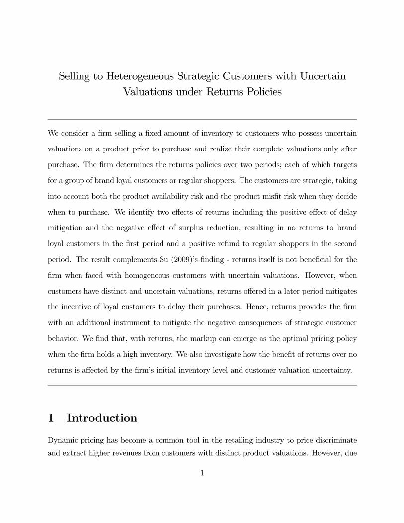
Figure 1: Relationship of optimal pricing policy and inventory level.

a price discount is offered in the later stage of the selling season. The markup pricing is

consistent with the practice of early promotion as a strategy to induce early purchases. Our

result suggests that with a high starting inventory level, the firm offer price promotion early

on, instead of waiting till the later stage of the season to do clearance sales.

The above proposition is silent when the inventory level is intermediate. As a remedy,

a numerical study suggests that as the inventory level increases, the firm’s optimal pricing

takes the form of markdown and then switches to markup. Figure 1 depicts how the price

difference changes in the inventory level for a representative example with the following

parameter values: the market size of each type of customers follows a Gamma distribution

with mean 100 for both types, and standard deviation 50 and 25 for the loyal customers and

regular shoppers respectively. The valuations of the loyal customers and regular shoppers

are uniformly distributed over [5, 10] and [3, 8], respectively.

14

6 Drivers of Benefits of Returns

We have shown that returns is beneficial for the firm because it serves as a strategic tool to

more effectively price discriminate customers who have heterogeneous and uncertain valua-

tions on the product. Concerning that there are administrative costs related to returns, it

is meaningful to understand to what extent returns policy outperforms no returns. To this

end, we identify two drivers and examine how each influences the benefits of returns.

6.1 Inventory Level

Let Πnrθ and Πrθ denote the optimal profit gained from the type-θ customers without returns

and with returns, respectively; θ ∈ {L, S}. Then

ΠnrL = pnr1 ENL min(NL, Q),

ΠnrS = pnr2 ENL,NS min(NS, (Q−NL)+),

ΠrL = pr1ENL min(NL, Q),

ΠrS = (pr2 − br2FS(br2))ENL,NS min(NS, (Q−NL)+),

where the optimal prices and the optimal refunds are characterized in Proposition 1 and

Proposition 2. Further, let Πnr and Πr be the firm’s optimal profit gained from both types

of customers without returns and with returns, respectively; then Πnr = ΠnrL + ΠnrS and

Πr = ΠrL +ΠrS.

Proposition 4 The firm earns lower profits from the regular shoppers with returns than

without returns. The opposite is true for the firm’s profits from the brand loyal customers.

That is, ΠrS ≤ ΠnrS and ΠrL ≥ ΠnrL .

The above proposition implies that offering returns to the regular shoppers reduces the

profits that the firm can earn from them. This result is due to the negative effect of surplus

reduction. However, returns improves the profits that the firm can earn from the brand loyal

15

customers, because of the positive effect of delay mitigation. Because the firm can adjust

the returns refund size to strike a balance of the tradeoff between the two effects, returns

improves the firm’s total profits, i.e., Πr ≥ Πnr.

Intuitively, the value of returns for the firm depends on the extent of the positive effect

of delay mitigation. As the firm’s starting inventory level Q increases, the shortage risk

decreases and the brand loyal customers’ incentive to delay purchase increases, resulting in a

stronger need to use returns as a strategic tool to deter delay purchase. Therefore, a higher

starting inventory level enhances the positive effect of delay mitigation and improves the

value of returns for the firm. This intuition is confirmed by the following analytical result.

Proposition 5 The firm’s gain in expected profits with returns relative to without returns,

i.e., Πr −Πnr, increases in the inventory level Q.

The literature has proposed the inventory rationing (i.e., deliberately installing a low

starting inventory level) as a strategic tool to deter strategic customers’ delay purchase

behavior. However, for products with lucrative profit margins, inventory rationing can be

very costly because of the high cost of demand loss. The above proposition implies that in

such situations, offering returns can be a good substitute of costly inventory rationing for

the firm to price discriminate customers and extract more values.

6.2 Customer Valuation Uncertainty

A key feature in our model is that the customer’s product valuation is uncertain prior

to purchase. Such uncertainty might arise due to the customer’s lack of experience and

unfamiliarity of some unknown features of the product, which might turn out to be well

appreciated or disliked by the customer after purchase. In such scenarios, the firm can

potentially reduce customer valuation uncertainty by providing the customer with better

access to product information such as in-store sales assistance, on-line peer reviews, free

samples, product demonstrations, etc. Therefore, an important question is whether or not the

firm can benefit from such valuation uncertainty reduction initiatives. Obviously, under the

16

no-returns policy, the customer valuation uncertainty has no impact on the firm’s expected

profit because the firm’s optimal prices and customers’ purchase decisions depend on the

customer product valuation only via the expected value (see Proposition 1). In contrast,

under the returns policy, the customer valuation uncertainty should have impacts on the

firm’s expected profit because it influences not only the customer’s purchase decision but also

the probability of product returns. Intuitively, the smaller valuation uncertainty decreases

the chance of customer returning the product, and thus leads to the firm’s lower cost of

returns. Therefore, one may conjecture that under the returns policy, the firm should benefit

from the reduction in customer valuation uncertainty. However, we show in this subsection

that the opposite is true.

Define v(1)θ = μθ + k1ε and v(2)θ = μθ + k2ε for θ = L, S, where μL > μS, k1 ≤ k2,

and ε is a random variable with zero mean and a finite support such that v(1)θ and v(2)θ are

nonnegative. Clearly, the customers with valuation v(1)L (for the brand loyal customer) and

v(1)S (for the regular shopper) have lower valuation uncertainty than those with v(2)L and v(2)S .

Let the firm’s expected profit under the optimal returns policy be Πr(k1) (Πr(k2)) when the

customer valuation uncertainty is low (high).

Proposition 6 The firm’s expected profit under the optimal returns policy is lower when the

customer valuation uncertainty is smaller. That is, Πr(k1) ≤ Πr(k2).

Proposition 6 provides a sharp result that the firm is hurt by a reduction in the customer

valuation uncertainty. The intuition is provided as follows. When the regular shoppers are

more uncertain about the product value and thus value more on returns, the firm can increase

the selling price in the second period so that the whole sales package is still attractive to

the regular shoppers. In doing so, it can make the sales package in the second period even

less appealing to the brand loyal customers because the incremental value they place on the

returns due to the increase of valuation uncertainty is less than that of the regular shoppers.

This implies that the increase in valuation uncertainty for both the loyal customers and

the regular shoppers strengthens the returns’ positive effect of delay mitigation, and hence

benefits the firm.

17

The above finding has an implication that the firm is actually worse off by providing

information or assistance to better inform its customers about the product features so as

to reduce valuation uncertainty, even if such information provision is costless to the firm.

However, this does not mean that information provision is useless. It is straightforward to

show that if such information provision is targeted only to the loyal customers, then the

firm is better off. Therefore, our finding suggests that the firm should provide product

information to a particular customer segment, not to every segment.

7 Conclusion

Our work reveals the behavioral role that returns plays in mitigating the negative conse-

quences of strategic customer behavior. We identify two effects of returns in dealing with

heterogeneous customers who are strategic and uncertain about the product value prior to

purchase: the negative effect of surplus reduction and the positive effect of delay mitigation.

Driven by the tradeoff of these two effects, the firm should offer a positive refund to regular

shoppers in the second period but no refund to brand loyal customers in the first period.

We find that under returns, the markup pricing policy can be optimal, implying that the

firm should offer early promotion instead of waiting to do clearance sales later on when the

firm has a high starting inventory level. We also identify two drivers of benefits of using

returns: the inventory level and the customer valuation uncertainty. We find that returns

is more beneficial when the inventory level is higher. While a reduction in the customer

valuation uncertainty has no impact on the firm’s profit under no returns, it hurts the firm

with returns.

Our work can be extended in several directions. The current model assumes that the

returned product cannot be resold to customers. When product resale is allowed, specifically,

the products sold and returned during the first period can be put into sales in the second

period, Su (2009) suggests that the optimal refund be equal to the resell value of the returned

product when customers are homogeneous. However, with heterogeneous customers, the

optimal refund in the first period should be lower than the resell value. The reason is that

18

the returned products are added up to the firm’s remaining inventory and thus increase

the product availability in a later period, strengthening the incentive for loyal customers

to delay purchases. Therefore, to counteract the strategic delay behavior, the firm should

lower the refund in the first period. Another extension would allow the inventory to be

determined endogenously. Because of its delay mitigation effect, returns can mitigate the

firm’s downward distortion in inventory ordering and thus improves the supply/demand

mismatch.

References

Aviv, Y., A. Pazgal. 2008. Optimal pricing of seasonal Products in the presence of forward-

looking consumers. Manufacturing and Service Operations Management 10(3): 339-359.

Cachon, G., R. Swinney. 2009. Purchasing, pricing and quick response in the presence of

strategic consumers. Management Science 55(3): 497-511.

Courty. P., H. Li. 2000. Sequential screening. Review of Economic Studies 67(4): 697-717.

Lai, G., L. Debo, K. Sycara. 2010. Buy now and match later: the impact of posterior price

matching on profit with strategic consumers. Manufacturing and Service Operations

Management 12(1): 33-55.

Li, C., F. Zhang. 2013. Advance demand information, price discrimination, and pre-order

strategies. Manufacturing and Service Operations Management 15(1): 57-71.

Liu, Q., G. van Ryzin. 2008. Strategic capacity rationing to induce early purchases. Man-

agement Science 54(6): 1115-1131.

Netessine, S., C. S. Tang. 2009. Consumer-Driven Demand and Operations Management

Models. Springer, New York.

Shen, Z., X. Su. 2007. Customer behavior modeling in revenue management and auctions: a

review and new research opportunities. Production and Operations Management 16(6):

713-728.

19

Su, X. 2007. Intertemporal pricing with strategic customer behavior. Management Science

53(5): 726-741.

Su, X. 2009. Consumer returns policies and supply chain performance. Manufacturing and

Service Operations Management 11(4): 595-612.

Swinney, R. 2011. Selling to strategic consumers when product value is uncertain: the value

of matching supply and demand. Management Science 57(10): 1737-1751.

Yin, R., Y. Aviv, A. Pazgal, C .S. Tang. 2009. Optimal markdown pricing: implications of

inventory display formats in the presence of strategic customers. Management Science

55(8): 1391-1408.

Zhang, D., W. L. Cooper. 2008. Managing clearance sales in the presence of strategic

customers. Production and Operations Management 17(4): 416-431.

AppendixProof of Proposition 1. We solve the firm’s problem (Pnr) in two cases. Case 1. The firm

serves the loyal customers in the first period and the regular shoppers in the second period,

i.e., θ = L and bθ = S. Case 2. The firm serves the regular shoppers in the first period and

the loyal customers in the second period, i.e., θ = S and bθ = L. We first derive the closedform expressions for the optimal prices in case 1, and then show that the firm earns higher

expected profits in case 1 than in case 2.

Consider the firm’s problem (Pnr) with θ = L and bθ = S. Let the optimal prices be pnr11

and pnr12 , and the firm’s optimal expected profit be Πnr1. We solve the firm’s problem in the

following three steps. First, it follows from the model assumption EvL ≥ EvS that (IC1) and(IR2) are sufficient to infer (IR1), implying that we can remove (IR1) from the constraints

without loss of optimality. Second, (IR2) must be binding at the optimal solution, because

otherwise the firm’s objective value can be improved by increasing p1 and p2 by a sufficiently

small amount without violating the constraints (IC1), (IC2), and (IR2). The binding (IR2)

constraint leads to pnr12 = EvS. Third, (IC1) must be binding at the optimal solution,

because otherwise the objective value can be improved by increasing p1 by a sufficiently small

amount without violating the constraints (IC1), (IC2), and (IR2). The binding constraint

20

(IC1) leads to pnr11 = EvL−z(EvL−EvS). Under the optimal prices pnr11 and pnr12 , the firm’s

expected profit is

Πnr1 = pnr11 ENL min(NL, Q) + pnr12 ENL,NS min(NS, (Q−NL)+). (1)

Next we turn the firm’s problem (Pnr) with θ = S and bθ = L. Let the optimal prices

be pnr21 and pnr22 , and the firm’s optimal expected profit be Πnr2. We will derive an upper

bound on Πnr2, and show that this upper bound is no larger than Πnr1. It follows from (IR1)

that pnr21 ≤ EvS =pnr12 . This, together with (IC2), implies that pnr22 ≤ EvL−(EvL−EvS)/z.Because z ≤ 1, we have pnr22 ≤ EvL−z(EvL−EvS) =pnr11 . Hence, we have the following

upper bound on Πnr2:

Πnr2 = pnr21 ENS min(NS, Q) + pnr22 ENL,NS min(NL, (Q−NS)+)

≤ pnr12 ENS min(NS, Q) + pnr11 ENL,NS min(NL, (Q−NS)+). (2)

By (1) and (2), we have

Πnr1 −Πnr2 ≥ pnr11 [ENL min(NL, Q)−ENL,NS min(NL, (Q−NS)+)]

−pnr12 [ENS min(NS, Q)−ENL,NS min(NS, (Q−NL)+)]

≥ pnr12 [ENL min(NL, Q)−ENL,NS min(NL, (Q−NS)+)]

−pnr12 [ENS min(NS, Q)−ENL,NS min(NS, (Q−NL)+)]

= 0

where the second inequality follows from the fact that pnr11 ≥ pnr12 and ENL min(NL, Q) −ENL,NS min(NL, (Q−NS)+) ≥ 0, and the last equality holds because

ENL min(NL, Q) +ENL,NS min(NS, (Q−NL)+) = ENL,NS min(NL +NS, Q)

21

and

ENS min(NS, Q) +ENL,NS min(NL, (Q−NS)+) = ENL,NS min(NL +NS, Q).

Therefore, the firm is better off by serving the loyal customers first, under which the optimal

prices are pnr1 = pnr11 = EvL−z(EvL−EvS) and pnr2 = pnr12 = EvS. This completes the

proof.

Proof of Proposition 2. We solve the firm’s problem (Pr) in two cases. Case 1. The firm

serves the loyal customers in the first period and the regular shoppers in the second period,

i.e., θ = L and bθ = S. Case 2. The firm serves the regular shoppers in the first period and

the loyal customers in the second period, i.e., θ = S and bθ = L. We first derive the closedform expressions for the optimal prices in case 1, and then show that the firm earns higher

expected profits in case 1 than in case 2.

Consider the firm’s problem (Pr) with θ = L and bθ = S. Let the optimal returns policiesbe (pr11 , b

r11 ) and (p

r12 , b

r12 ), and the firm’s optimal expected profit be Π

r1. Using the same

arguments for the case 1 in the proof of Proposition 1, we can show that both the constraints

(IC1) and (IR2) are binding. This leads to

p2 = EvS max(vS, b2) (3)

and

p1 = EvL max(vL, b1)−z[EvL max(vL, b2)− EvS max(vS, b2)]. (4)

Substituting p1 and p2 by the right hand side of (3) and (4), respectively, we can rewrite

the firm’s objective function as

maxb1≥0,b2≥0

{[EvL max(vL, b1)− b1FL(b1)−z[EvL max(vL, b2)

−EvS max(vS, b2)]]ENL min(NL, Q)

+[EvS max(vS, b2)− b2FS(b2)]ENL,NS min(NS, (Q−NL)+)},

22

implying that the optimal returns refunds are br11 = 0 and

br12 = argmaxb2≥0

{[EvS max(vS, b2)− b2FS(b2)]ENL,NS min(NS, (Q−NL)+)

−z[EvL max(vL, b2)−EvS max(vS, b2)]ENL min(NL, Q)}.

This, together with (3) and (4), determines pr11 and pr22 . It is verifiable that the solution

{(pr11 , br11 ), (pr12 , br12 )} satisfies the constraint (IC2), and thus is the optimal solution to theproblem (Pr) with θ = L and bθ = S.Next we turn the problem (Pr) with θ = S and bθ = L. Let the optimal returns policies

be (pr21 , br21 ) and (p

r22 , b

r22 ), and the firm’s optimal expected profit be Π

r2. Following the same

arguments of case 2 in the proof of Proposition 1, we have

p1 ≤ EvS max(vS, b1)

and

p2 ≤ EvL max(vL, b2)−z[EvL max(vL, b1)−EvS max(vS, b1)].

Hence, we have the following upper bound on Πr2:

Πr2 ≤ maxb1≥0,b2≥0

{[EvS max(vS, b1)− b1FS(b1)]ENS min(NS, Q) + [EvL max(vL, b2)− b2FL(b2)

−z[EvL max(vL, b1)−EvS max(vS, b1)]]ENL,NS min(NL, (Q−NS)+)}

= maxb1≥0

{[EvS max(vS, b1)− b1FS(b1)]ENS min(NS, Q)

+[EvL −z[EvL max(vL, b1)− EvS max(vS, b1)]]ENL,NS min(NL, (Q−NS)+)}

= [EvS max(vS, br21 )− br21 FS(br21 )]ENS min(NS, Q)

+[EvL −z[EvL max(vL, br21 )−EvS max(vS, br21 )]]ENL,NS min(NL, (Q−NS)+)}.

23

Recall that

Πr1 = maxb2≥0

{[EvL −z[EvL max(vL, b2)−EvS max(vS, b2)]]ENL min(NL, Q)

+[EvS max(vS, b2)− b2FS(b2)]ENL,NS min(NS, (Q−NL)+)}

≥ [EvL −z[EvL max(vL, br21 )− EvS max(vS, br21 )]]ENL min(NL, Q)

+[EvS max(vS, br21 )− br21 FS(br21 )]ENL,NS min(NS, (Q−NL)+)

Hence,

Πr1 −Πr2

≥ [EvL −z[EvL max(vL, br21 )− EvS max(vS, br21 )]][ENL min(NL, Q)

−ENL,NS min(NL, (Q−NS)+)]

−[EvS max(vS, br21 )− br21 FS(br21 )][ENS min(NS, Q)− ENL,NS min(NS, (Q−NL)+)]

≥ [EvS max(vS, br21 )− br21 FS(br21 )][ENL min(NL, Q)−ENL,NS min(NL, (Q−NS)+)]

−[EvS max(vS, br21 )− br21 FS(br21 )][ENS min(NS, Q)− ENL,NS min(NS, (Q−NL)+)]

= 0,

where the second inequality is due to

EvL − [EvS max(vS, br21 )− br21 FS(br21 )]

≥ EvL max(vL, br21 )− br21 FL(br21 )− [EvS max(vS, br21 )− br21 FS(br21 )]

≥ z[EvL max(vL, br21 )−EvS max(vS, br21 )].

This completes the proof.

Proof of Proposition 3. Recall from Proposition 2 that pr1 = EvL −z[EvL max(vL, br2)−EvS max(vS, b

r2)] and p

r2 = EvS max(vS, b

r2). As Q goes to zero, z goes to 0. By the definition

of br2 in Proposition 2, br2 also goes to zero, implying that p

r1 − pr2 goes to EvL−EvS > 0.

This implies that there exists Q such that pr1 > pr2 for Q ≤ Q. As Q goes to infinity, z goes

24

to 1, and thus pr1 − pr2 goes to EvL −EvL max(vL, br2) < 0, implying that there exists Q suchthat pr1 > p

r2 for Q ≥ Q.

Proof of Proposition 4. The proposition follows from the definition of ΠrS, ΠnrS , Π

nrL , and

ΠrL:

ΠrS = (pnr2 − br2FS(br2))ENL,NS min(NS, (Q−NL)+)

= (EvS max(vS, br2)− br2FS(br2))ENL,NS min(NS, (Q−NL)+)

≤ EvSENL,NS min(NS, (Q−NL)+)

= pnr2 ENL,NS min(NS, (Q−NL)+)

= ΠnrS ,

and

ΠnrL = pnr1 ENL min(NL, Q)

= [EvL−z(EvL−EvS)]ENL min(NL, Q)

≤ [EvL −z[EvL max(vL, br2)−EvS max(vS, br2)]]ENL min(NL, Q)

= ΠrL.

25

Proof of Proposition 5. By definition of Πr and Πnr, we have

Πr −Πnr

= [EvL −z[EvL max(vL, br2)−EvS max(vS, br2)]]ENL min(NL, Q)

+[EvS max(vS, br2)− br2FS(br2)]ENL,NS min(NS, (Q−NL)+)

−[EvL−z[EvL −EvS]]ENL min(NL, Q)−EvSENL,NS min(NS, (Q−NL)+)

= zENL min(NL, Q)[EvL −EvS − [EvL max(vL, br2)−EvS max(vS, br2)]]

−[EvS − [EvS max(vS, br2)− br2FS(br2)]]ENL,NS min(NS, (Q−NL)+)

= ENL,NS min(NS, (Q−NL)+){(ENL min(NL, Q)/ENS)[EvL −EvS−[EvL max(vL, br2)−EvS max(vS, br2)]]− [EvS − [EvS max(vS, br2)− b2FS(br2)]]}

which increases in Q because both ENL,NS min(NS, (Q − NL)+) and ENL,NS min(NS, (Q −NL)

+) increase in Q.

Proof of Proposition 6. Let the firm’s expected profit under the optimal returns policy

be Πr(k) when the product valuations of the loyal customers and of the regular shoppers

are given by vL = μL + kε and vS = μS + kε. Let g and G be the density and distribution

function of ε. Let b(k) be the optimal returns refund in the second period. It follows from

the definition of Πr(k) that

Πr(k) = [μL −z[Eεmax(μL + kε, b(k))−Eεmax(μS + kε, b(k))]]ENL min(NL, Q)

+[Eεmax(μS + kε, b(k))− b(k)G(b(k)− μS

k)]ENL,NS min(NS, (Q−NL)+).

26

Taking the derivative of Πr(k) with respect to k, we have

∂Πr(k)/∂k

=

"Z +∞

b(k)−μSk

εg(ε)dε−Z +∞

b(k)−μLk

εg(ε)dε

#zENL min(NL, Q)

+

"b(k)− μS

k2b(k)g(

b(k)− μSk

) +

Z +∞

b(k)−μSk

εg(ε)dε

#ENL,NS min(NS, (Q−NL)+). (5)

It suffices to prove that ∂Πr(k)/∂k ≥ 0. Because b(k) is the maximizer over [0,+∞), itfollows from the first-order necessary condition that

∙G(b(k)− μS

k)−G(b(k)− μL

k)

¸zENL min(NL, Q)

≤ b(k)

kg(b(k)− μS

k)ENL,NS min(NS, (Q−NL)+). (6)

By (5) and (6), we have

∂Πr(k)/∂k

≥"−Z b(k)−μS

k

b(k)−μLk

εg(ε)dε+b(k)− μS

k

∙G(b(k)− μS

k)−G(b(k)− μL

k)

¸#zENL min(NL, Q)

+

"Z +∞

b(k)−μSk

εg(ε)dε

#ENL,NS min(NS, (Q−NL)+)

=

"Z b(k)−μSk

b(k)−μLk

∙b(k)− μS

k− ε

¸g(ε)dε

#zENL min(NL, Q)

+

"Z +∞

b(k)−μSk

εg(ε)dε

#ENL,NS min(NS, (Q−NL)+)

≥ 0.

where the last inequality holds becauseR b(k)−μS

kb(k)−μL

k

hb(k)−μS

k− εig(ε)dε ≥ 0 and

R +∞b(k)−μS

k

εg(ε)dε ≥0 (since Eε = 0).

27