Self-organizing maps in manifolds with complex topologies ...

SELF ORGANIZING SEMANTIC
TOPOLOGIES IN PEER DATABASE
SYSTEMS
AMI EYAL

SELF ORGANIZING SEMANTIC TOPOLOGIES
IN PEER DATABASE SYSTEMS
RESEARCH THESIS
SUBMITTED IN PARTIAL FULFILLMENT OF THE
REQUIREMENTS
FOR THE DEGREE OF MASTER OF SCIENCE
IN INFORMATION MANAGEMENT ENGINEERING
AMI EYAL
SUBMITTED TO THE SENATE OF THE TECHNION — ISRAEL INSTITUTE OF TECHNOLOGY
TAMMUZ, 5767 HAIFA JUNE, 2007

THIS RESEARCH THESIS WAS SUPERVISED BY DR. AVIGDOR GAL
UNDER THE AUSPICES OF THE INDUSTRIAL ENGINEERING AND
MANAGEMENT DEPARTMENT
ACKNOWLEDGMENT
I would like to express my deepest gratitude to my supervisor, Pro-
fessor Avigdor Gal, for his devoted guidance and wise counsel. My
sincere thanks to the faculty personnel, for their help in all practical
and administrative matters during my studies, special thanks are given
to Judith Ish-Lev. Additional thanks to my colleagues, Haggai, Inbal,
Victor and others, for helpful discussions, motivation and support when
I most needed it. Last and most important, I am deeply indebted to
my dear family and friends, whose endless love and support enabled
the completion of this work.
THE GENEROUS FINANCIAL HELP OF THE EUROPEAN COMMISSION
SIXTH FRAMEWORK IST PROJECT QUALEG AND THE TECHNION IS
GRATEFULLY ACKNOWLEDGED

Contents
Abstract xi
List of Symbols 1
1 Introduction 3
1.1 Related Work . . . . . . . . . . . . . . . . . . . . . . . . . . . . . . . 5
1.1.1 Schema Matching . . . . . . . . . . . . . . . . . . . . . . . . 5
1.1.2 Peer Database Systems . . . . . . . . . . . . . . . . . . . . . 7
1.2 Thesis Outline . . . . . . . . . . . . . . . . . . . . . . . . . . . . . . 11
1.3 Contributions . . . . . . . . . . . . . . . . . . . . . . . . . . . . . . . 12
2 Model Definition 14
2.1 The Data Model . . . . . . . . . . . . . . . . . . . . . . . . . . . . . 15
2.2 The Network Model . . . . . . . . . . . . . . . . . . . . . . . . . . . 16
2.2.1 Schema Mappings . . . . . . . . . . . . . . . . . . . . . . . . 16
2.2.2 Query Dissemination . . . . . . . . . . . . . . . . . . . . . . . 18
2.2.3 Semantic Topology . . . . . . . . . . . . . . . . . . . . . . . . 20
2.3 The Matching Model . . . . . . . . . . . . . . . . . . . . . . . . . . . 21
2.3.1 Mapping Accuracy . . . . . . . . . . . . . . . . . . . . . . . . 22
iii

CONTENTS iv
2.3.2 Mapping Accuracy Preservation . . . . . . . . . . . . . . . . 26
2.4 Evaluation of semantic topologies . . . . . . . . . . . . . . . . . . . . 31
2.4.1 Self-Interest Based Topology Evaluation . . . . . . . . . . . . 32
2.4.2 Cooperative Interest Based Topology Evaluation . . . . . . . 34
3 On Optimal Semantic Topologies 37
3.1 Optimal Self-Interest Based Topologies . . . . . . . . . . . . . . . . . 38
3.2 Optimal Cooperative-Interest Based Topologies . . . . . . . . . . . . 40
3.2.1 Degree Bounded Maximum Minimal Product Paths Tree (db-
MMPT) . . . . . . . . . . . . . . . . . . . . . . . . . . . . . . 42
3.2.2 Single Peer Single Query (SPSQ) Optimal Topology Problem 50
3.3 Discussion . . . . . . . . . . . . . . . . . . . . . . . . . . . . . . . . 52
4 Dynamic Self-Organizing Topologies 54
4.1 Semantic Acquaintance . . . . . . . . . . . . . . . . . . . . . . . . . 55
4.2 Semantic Replacement . . . . . . . . . . . . . . . . . . . . . . . . . . 61
5 Experiments 67
5.1 Simulation Architecture . . . . . . . . . . . . . . . . . . . . . . . . . 67
5.2 Data and parameters . . . . . . . . . . . . . . . . . . . . . . . . . . . 72
5.3 Experimental setup . . . . . . . . . . . . . . . . . . . . . . . . . . . 75
5.4 Evaluation . . . . . . . . . . . . . . . . . . . . . . . . . . . . . . . . 76
5.5 Results . . . . . . . . . . . . . . . . . . . . . . . . . . . . . . . . . . 78
5.5.1 Good Initial Topologies . . . . . . . . . . . . . . . . . . . . . 78
5.5.2 Initial Bad Topologies . . . . . . . . . . . . . . . . . . . . . . 82
5.5.3 Randomly Generated Topologies . . . . . . . . . . . . . . . . 92

CONTENTS v
5.6 Discussion . . . . . . . . . . . . . . . . . . . . . . . . . . . . . . . . 105
6 Discussion 109
6.1 Conclusions . . . . . . . . . . . . . . . . . . . . . . . . . . . . . . . . 109
6.2 Future Work . . . . . . . . . . . . . . . . . . . . . . . . . . . . . . . 110
References 111
Hebrew Abstract k

List of Figures
2.1 A query reformulation example. . . . . . . . . . . . . . . . . . . . . . 17
2.2 DPMS model description. . . . . . . . . . . . . . . . . . . . . . . . . 18
2.3 A semantic network graph, where peers’ schemata are interlinked by
schema mappings provided by the peers. . . . . . . . . . . . . . . . . 19
2.4 Semantic Network Model: Query translation layers and a Topology
with a limit of Kp = 2 neighbors. . . . . . . . . . . . . . . . . . . . . 21
2.5 An example of mapping accuracy. . . . . . . . . . . . . . . . . . . . . 24
2.6 An example of mapping preservation. . . . . . . . . . . . . . . . . . . 28
2.7 An example for query reformulation graph. . . . . . . . . . . . . . . . 30
2.8 An example for accuracy oriented semantic topology evaluation. . . . 33
3.1 Classification of the optimal CIV topology problem. . . . . . . . . . 41
3.2 Example for maximum minimal product paths tree (MMPT) and max-
imum product paths tree (MPT). . . . . . . . . . . . . . . . . . . . . 44
3.3 Example of transformation from MPT to SPT. . . . . . . . . . . . . . 46
3.4 Example of MMPT Vs. db-MMPT. . . . . . . . . . . . . . . . . . . . 47
3.5 Example of transformation from ATSP to db-MMPT. . . . . . . . . . 50
3.6 Example of transformation from db-MMPT to SPSQ. . . . . . . . . . 52
vi
LIST OF FIGURES vii
4.1 Semantically disconnected components. . . . . . . . . . . . . . . . . . 56
4.2 Acquaintance policies example. . . . . . . . . . . . . . . . . . . . . . 60
4.3 Bad replacement example. . . . . . . . . . . . . . . . . . . . . . . . . 63
5.1 Simulation Model: domain, schemata, and query sets. . . . . . . . . . 68
5.2 Simulation Model: semantic topology and query translation layers. . . 70
5.3 Simulation Model: sequence Diagram of a single query cycle. . . . . . 71
5.4 Domain attributes probability for participation in peer schemas and
queries. . . . . . . . . . . . . . . . . . . . . . . . . . . . . . . . . . . 73
5.5 Attributes mapping accuracies distributions for similar and different
attributes. . . . . . . . . . . . . . . . . . . . . . . . . . . . . . . . . . 74
5.6 Network topology: out degree Vs. peer rank following power law. . . 74
5.7 Replacement policies comparison: convergence in initial good topologies 79
5.8 Replacement policies comparison: topology changes in initial good
topologies . . . . . . . . . . . . . . . . . . . . . . . . . . . . . . . . . 80
5.9 Replacement policies comparison: SIV change in initial good topologies 81
5.10 Replacement policies comparison: CIV change in initial good topologies 81
5.11 Acquaintance policies comparison: convergence in initial bad topologies 83
5.12 Acquaintance policies comparison: topology changes in initial bad
topologies . . . . . . . . . . . . . . . . . . . . . . . . . . . . . . . . . 84
5.13 Acquaintance policies comparison: SIV change in initial bad topologies 84
5.14 Acquaintance policies comparison: CIV change in initial bad topologies 85
5.15 Acquaintance policies comparison: reachability change in initial bad
topologies . . . . . . . . . . . . . . . . . . . . . . . . . . . . . . . . . 86

LIST OF FIGURES viii
5.16 Acquaintance policies comparison: average CIV measure change in
initial bad topologies . . . . . . . . . . . . . . . . . . . . . . . . . . . 86
5.17 Replacement policies comparison: convergence in initial bad topologies 87
5.18 Replacement policies comparison: topology changes in initial bad topologies 88
5.19 Replacement policies comparison: SIV change in initial bad topologies 89
5.20 Replacement policies comparison: CIV change in initial bad topologies 90
5.21 Replacement policies comparison: average CIV measure change . . . 90
5.22 Replacement policies comparison: reachability change in initial bad
topologies . . . . . . . . . . . . . . . . . . . . . . . . . . . . . . . . . 91
5.23 Acquaintance policies comparison: convergence in randomly generated
topologies . . . . . . . . . . . . . . . . . . . . . . . . . . . . . . . . . 93
5.24 Acquaintance policies comparison: topology changes in randomly gen-
erated topologies . . . . . . . . . . . . . . . . . . . . . . . . . . . . . 94
5.25 Acquaintance policies comparison: SIV change in randomly generated
topologies . . . . . . . . . . . . . . . . . . . . . . . . . . . . . . . . . 95
5.26 Acquaintance policies comparison: CIV change in randomly generated
topologies . . . . . . . . . . . . . . . . . . . . . . . . . . . . . . . . . 96
5.27 Acquaintance policies comparison: average CIV change in randomly
generated topologies . . . . . . . . . . . . . . . . . . . . . . . . . . . 96
5.28 Acquaintance policies comparison: reachability change in randomly
generated topologies . . . . . . . . . . . . . . . . . . . . . . . . . . . 97
5.29 Replacement policies comparison: convergence in randomly generated
topologies . . . . . . . . . . . . . . . . . . . . . . . . . . . . . . . . . 98
5.30 Replacement policies comparison: number of topology changes in ran-
domly generated topologies . . . . . . . . . . . . . . . . . . . . . . . . 99

LIST OF FIGURES ix
5.31 Replacement policies comparison: SIV change in random topologies . 100
5.32 Replacement policies comparison: CIV change in random topologies . 101
5.33 Replacement policies comparison: average CIV change in random
topologies . . . . . . . . . . . . . . . . . . . . . . . . . . . . . . . . . 102
5.34 Replacement policies comparison: reachability change in random topologies103
5.35 Replacement policies comparison: topology change visualization . . . 104
5.36 SIV Vs. Average CIV in randomly generated topologies . . . . . . . . 106

List of Tables
4.1 Acquaintance policies evaluation measures . . . . . . . . . . . . . . . 61
4.2 Mapping accuracies for selected candidates using different acquain-
tance policies . . . . . . . . . . . . . . . . . . . . . . . . . . . . . . . 62
4.3 Replacement policies evaluation measures . . . . . . . . . . . . . . . . 65
5.1 Simulation parameters . . . . . . . . . . . . . . . . . . . . . . . . . . 72
5.2 Summary of experimental setup parameters . . . . . . . . . . . . . . 75
x

Abstract
Peer database management systems (PDMS) combine the decentralized setting and
autonomy of peer-to-peer systems with the rich semantic context of database systems.
In a PDMS, members use schema matching techniques to establish schema mappings
as the basis for peer querying. The large-scale and dynamic environments of peer-
to-peer networks dictate the use of automatic schema matching, which was shown to
carry with it a degree of uncertainty.
In the first part of this thesis, we introduce a model for a PDMS that considers
the inherent uncertainty of automatic schema matching and the increase of this un-
certainty over transitive matching in a decentralized environment. We examine the
query reformulation quality in our model, influenced by the use of variant semantic
network topologies. We analyze both local interest and global welfare of semantic
topologies.
Next, we consider (offline) problems of finding optimal semantic topologies that
maximize query reformulation quality. We present an algorithm to find such optimal
topologies that maximize peers local interest. We also show that even in the pres-
ence of complete offline network knowledge, the problem of finding a topology that
maximizes the global welfare is NP-Complete even for a very simple setting.
In the third part, we consider the (online) setting of a peer to peer system where no
xi

ABSTRACT xii
single peer obtains complete network knowledge. We present several heuristic (online)
algorithms for topology self organization in the absence of full network knowledge.
In the final part, we present a PDMS simulation using our model and our online
algorithms for topology self-organization. We compared our algorithms with simi-
lar algorithms in the context of peer file-sharing systems. Our results indicate that
our algorithms better exploit interest-based locality in PDMS environment. We also
show experimental results indicating that local interest interferes with global welfare
in the context of optimal topology self establishment. Finally, we show that opti-
mal topologies maximizing global welfare can not be reached by independent peers
individually applying self organization algorithms, but rather require collaborative
algorithms applied by peers in cooperation.

List of Symbols
P :Set of peers in a PDMS
p :Single peer
DBp :Peer p’s database
Sp :Peer p’s database descriptive schema
S :Set of peers schemata in a PDMS
A :Schema attribute
AI :Set of attribute interpretations
∆I :Global domain of attribute interpretations
q(Si) :Query formed in terms of schema Si
Qp :Set of queries issued by peer p
λq :Query q appearance frequency
IDp :Peer p’s network identifier
mAi→Aj:Attribute mapping from Ai to Aj
MSi→Sj:Schema mapping from Si to Sj
M :Set of schema mappings in a PDMS
G(P, M) :Semantic graph with a set of peers P and a set of mappings M
T (P ,M) :Semantic topology with a set of peers P and a set of mappings M
1

LIST OF SYMBOLS 2
Np :Set of peer p’s neighbors in a semantic topology
Kp :Peer p’s maximum neighbors boundary
µ :Mapping accuracy confidence measure
PathSi→Sj:Path of transitive schema mappings
α :Accuracy preservation over a path of transitive schema mappings
SIV :Self-interest value measure for semantic topology evaluation
CIV :Cooperative-interest value measure for semantic topology evaluation

Chapter 1
Introduction
Peer-to-peer (P2P) systems have served as the subject of a wide research effort over
the past few years. Advantages such as scalability, autonomy and robustness made
it useful in various domains, and many practical applications using this technology
proved most successful. Originally, P2P systems supported only a simple data model
and limited query expressiveness. Later, some research efforts were made to enrich
P2P data models with meta data and enhance query expressiveness [50, 60, 36].
Recently, a revolutionary approach suggested an integration of P2P and database
management systems (DBMS) technologies.
Peer database management systems (PDMS) combine the decentralized setting
and autonomy of P2P systems with the rich semantic context of database management
systems. Each peer maintains a local database and a descriptive schema exposing its
database to the other peers. Information sharing is done by means of query dissem-
ination, iterative propagation of queries among connected peers. Expressive query
languages of the type used in database management systems (e.g. SQL, XQuery)
3

CHAPTER 1. INTRODUCTION 4
may be used to compose complex queries. In a PDMS, members use schema match-
ing techniques to establish schema mappings as the basis for peer querying. Queries
are being reformulated from a source to target peers schema using these mappings.
Schema matching is the process of matching between concepts describing the
meaning of data in heterogeneous schemata. Schema mapping, the outcome of a
matching process, is a translation between similar concepts in a source and target
schemata and may be used for reformulation of queries issued using terms of one
schema to another. Due to its complexity, the operation of matching between two
heterogeneous schemata, was originally performed by human experts [14, 37]. How-
ever, the large-scale and dynamic environments of peer-to-peer networks dictate the
use of automatic schema matching. Automatic schema matching process was shown
to carry with it a degree of uncertainty and its outcome may contain inaccurate,
possibly erroneous mappings.
The presence of uncertain mappings between the peers impacts the quality of
reformulated queries and their returned results. Queries using inaccurate mappings
may return irrelevant results. Consider for example a schema mapping where attribute
FamilyName in one schema is inaccurately mapped to attribute FirstName in another
schema; The simple query return all persons with family name=’Smith’ would then
be translated to return all persons with first name=’Smith’, thus yeilding with results
irrelevant to the original query. Selection of schema mappings by individual peers
influences therefore the overall quality of the query process. In a P2P environment
such as PDMS, mapping selection is derived from the network topology, i.e. the
selection of neighbors by individual peers. A wise choice of neighbors may reduce the
uncertainty of schema mappings and as a direct result, may reduce the inaccuracy of
queries and increase the quality of their outcome.

CHAPTER 1. INTRODUCTION 5
In this thesis we consider a setting of a PDMS with matching uncertainty. Schema
mappings created by matching between peers are inaccurate to some degree. We con-
sider a dynamic setting where peer connects with some arbitrary peers upon joining
the network and can later change its neighbor set selection. Given this setting, we
focus on the following questions:
• Can we efficiently identify “good” topologies, those that reduce the uncertainty
in the network?
• Can such “good” topologies self organize by self-interested peers acting individ-
ually?
1.1 Related Work
We divide this section into two main subsections: in Section 1.1.1 we bring related
work in the field of schema matching and in Section 1.1.2 we discuss related work in
the field of P2P and specifically PDMSs.
1.1.1 Schema Matching
Schema matching is recognized to be one of the basic operations required by the
process of data and schema integration [8, 42, 12], and thus has a great impact on
its outcome. Schema mappings can serve in tasks of targeted content delivery, view
integration, database integration, query rewriting over heterogeneous sources, dupli-
cate data elimination, and automatic streamlining of workflow activities that involve
heterogeneous data sources. As such, schema matching has impact on numerous mod-
ern applications, currently suffering from the lack of ability to easily and effectively

CHAPTER 1. INTRODUCTION 6
organize their dataspaces [26]. It impacts business, where company data sources con-
tinuously realign due to changing markets. It also impacts the way business and other
information consumers seek information over the Web. Finally, it also impacts life
sciences, where scientific workflows cross system boundaries more often than not.
Research into schema matching has been going on for more than 25 years now (see
surveys [8, 59, 55, 61] and various online lists, e.g., OntologyMatching1, Ziegler2, Dig-
iCULT3, and SWgr4,) first as part of a broader effort of schema integration and then
as a standalone research. Due to its cognitive complexity, schema matching has been
traditionally considered to be AI-complete, performed by human experts [14, 37]. For
obvious reasons, manual concept reconciliation in large scale and/or dynamic envi-
ronments (with or without computer-aided tools) is inefficient and at times close to
impossible. The move from manual to semi-automatic schema matching has been jus-
tified in the literature using arguments of scalability (especially for matching between
large schemata [34]) and by the need to speed-up the matching process. Researchers
also argue for moving to fully-automatic (that is, unsupervised) schema matching in
settings where a human expert is absent from the decision process. In particular,
such situations characterize numerous emerging applications triggered by the vision
of the Semantic Web and machine-understandable Web resources [10, 63]. In these
applications, schema matching is no longer a preliminary task to the data integration
effort, but rather ad-hoc and incremental.
The AI-complete nature of the problem dictates that semi-automatic and auto-
matic algorithms for schema matching will be of heuristic nature at best. Over the
1http://www.ontologymatching.org/2http://www.ifi.unizh.ch/˜pziegler/IntegrationProjects.html3http://www.digicult.info/pages/resources.php?t=104http://www.semanticweb.gr/modules.php?name=News&
file=categories&op=newindex&catid=17

CHAPTER 1. INTRODUCTION 7
years, a significant body of work was devoted to the identification of schema match-
ers, heuristics for schema matching. Examples of algorithmic tools providing means
for schema matching include COMA [19], Cupid [45], OntoBuilder [29], Autoplex [9],
Similarity Flooding [47], Clio [48], Glue [21], to name just a few. The main objective
of schema matchers is to provide schema mappings that will be effective from the user
point of view, yet computationally efficient (or at least not disastrously expensive).
Such research has evolved in different research communities, including databases,
information retrieval, information sciences, data semantics, and others.
Automatic matching algorithms, based on syntactic, rather than semantic, means,
may carry with it a degree of uncertainty. [30] used a fuzzy framework to model the
uncertainty of the matching process outcome. They introduced a confidence mea-
sure associated with a matching outcome, indicating a matching algorithm’s belief in
the accuracy of the received mapping. High confidence value indicates an accurate
mapping, close to the perfect outcome of a human expert matching. In addition,
they demonstrated through theoretical and empirical analysis that for a certain fam-
ily of “Well-behaved” mappings termed monotonic, one can safely interpret a high
confidence measure as a good semantic mapping. Thus, automatic matching algo-
rithms applying mappings maintaining the monotonicity principle, can be trusted to
associate confidence measures truly reflecting the accuracy of their outcome.
1.1.2 Peer Database Systems
P2P networks suggest a model where participants communicating via ad-hoc connec-
tions share resources to offer some collaborative service. In contrast with classical
client/server application, all the peer nodes in the network simultaneously function
as both clients and servers to the other nodes in the network. Advantages of this

CHAPTER 1. INTRODUCTION 8
decentralized setting such as scalability, autonomy and robustness made it useful
for various domains and applications: USENET [35] was an early P2P system for
propagation of news articles. BitTorrent5 is a P2P network for file content sharing
(e.g. audio, video, data, etc...), Skype6 is a P2P based Internet telephony system and
TVants7 is a video streaming (TV) distribution system based on P2P technology.
Peers in P2P networks are typically organized in an overlay network, a structure
built on top of another network such as the Internet. P2P networks can be classified
according to their overlay network organization: unstructured P2P systems such as
Gnutella [1] are constructed by peers establishing arbitrary links with a fixed number
of other peers. In an unstructured P2P network, queries for data have to be flooded
through the network in order to find peers sharing the data. Query propagation is
regulated by a Time-To-Live (TTL) value, indicating the period of time or number of
iterations for query forwarding, before being discarded; this simple robust mechanism
restricts query broadcast within a certain radius. Hence, the main disadvantages with
such networks is that search mechanism is highly inefficient due to flooding and may
fail to retrieve relevant results under TTL limitation.
Research efforts in the context of this problem in file sharing P2P systems, sug-
gested the use of topology self organization as a possible solution. Under this ap-
proach, peers apply light-weight algorithms for estimation of semantic relation with
other peers and links in the overlay network are adjusted in order to improve search
performance. In [68], light-weight policies such as LRU and History were suggested
to identify and maintain links to a list of semantically close neighbors. [62] suggested
the creation of interest-based shortcuts, i.e. direct links to peers with high likelihood
5http://www.bittorrent.com6http://www.skype.com/7http://www.tvants.com
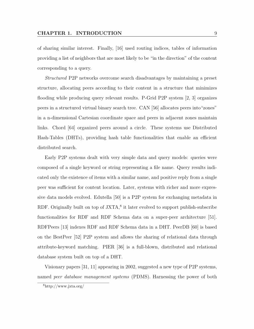
CHAPTER 1. INTRODUCTION 9
of sharing similar interest. Finally, [16] used routing indices, tables of information
providing a list of neighbors that are most likely to be “in the direction” of the content
corresponding to a query.
Structured P2P networks overcome search disadvantages by maintaining a preset
structure, allocating peers according to their content in a structure that minimizes
flooding while producing query relevant results. P-Grid P2P system [2, 3] organizes
peers in a structured virtual binary search tree. CAN [56] allocates peers into“zones”
in a n-dimensional Cartesian coordinate space and peers in adjacent zones maintain
links. Chord [64] organized peers around a circle. These systems use Distributed
Hash-Tables (DHTs), providing hash table functionalities that enable an efficient
distributed search.
Early P2P systems dealt with very simple data and query models: queries were
composed of a single keyword or string representing a file name. Query results indi-
cated only the existence of items with a similar name, and positive reply from a single
peer was sufficient for content location. Later, systems with richer and more expres-
sive data models evolved. Edutella [50] is a P2P system for exchanging metadata in
RDF. Originally built on top of JXTA,8 it later evolved to support publish-subscribe
functionalities for RDF and RDF Schema data on a super-peer architecture [51].
RDFPeers [13] indexes RDF and RDF Schema data in a DHT. PeerDB [60] is based
on the BestPeer [52] P2P system and allows the sharing of relational data through
attribute-keyword matching. PIER [36] is a full-blown, distributed and relational
database system built on top of a DHT.
Visionary papers [31, 11] appearing in 2002, suggested a new type of P2P systems,
named peer database management systems (PDMS). Harnessing the power of both
8http://www.jxta.org/

CHAPTER 1. INTRODUCTION 10
P2P and database management technologies, they introduced a vision of a decen-
tralized network of autonomous information sources, each maintaining a rich expres-
sive data model and query capabilities. Integrating these two worlds, they offered a
large-scale robust network of peers with rich heterogeneous schemata where schema
mappings, used as a semantic glue connecting peers in the network, enable peers to
cooperate and share information by means of query reformulation. Query dissemina-
tion in PDMS is done by means of gossiping [5], iterative query reformulation between
connected peers, similar to query propagation in unstructured P2P systems.
The Piazza project [33, 32, 66] introduced a PDMS network where peers schemata
are interlinked by GLAV mappings. Piazza focused on the logic structure, algorith-
mic, and implementation aspects of peer data management such as definition and
creation of mappings, query reformulation and propagation, and methods to improve
their efficiency [65]. The Hyperion project [7, 40] presented another PDMS relying
on the Local Relational Model (LRM) [58], using instance level mappings and co-
ordination rules to share data in decentralized environments. They also focused on
implementation aspects such as mappings definition using mapping tables [46] and al-
gorithms for query reformulation computing [39]. Both Piazza and Hyperion consider
schema mappings as most-accurate as if created by a human expert. [6] first real-
ized the effect of matching uncertainty on query reformulation accuracy and offered
an extended model of PDMS, including confidence measures representing mapping
accuracies. They suggest the usage of mapping accuracy measure for selective query
routing. However, they do not assume the use of matching algorithm following the
monotonicity principle, and hence provide algorithms integrated into the query mech-
anism for analysis and update of mapping confidence measures. Their approach can
be viewed as complementary to ours.
CHAPTER 1. INTRODUCTION 11
1.2 Thesis Outline
In this thesis, we model a PDMS as a network of peers connected by schema mapping
links associated with mapping confidence measures. We assume matching algorithms
follow the monotonicity principle and take confidence measure as truly reflecting
mapping accuracy. We model the deterioration of accuracy over transitive mappings
and its impact on query processing in PDMS. We define a PDMS semantic overlay
structure, namely semantic topology and show the influence of topology selection on
the quality of queries reformulation in a PDMS. Finally, we adopt the approach of
overlay (topology) self organization in search of semantic topologies that maximize
reformulation quality.
The remaining of this thesis is organized as follows:
In Chapter 2 we present our formal PDMS model. We describe the local database
maintained by each peer, the semantic network of peers connected via schema map-
pings, and elaborate on schema mappings characteristics and their influence on query
mechanism. Additionally, we introduce the semantic topology concept, the organiza-
tion of matched peers in the semantic network and suggest evaluation measures for
semantic topologies in the context of uncertain mappings in PDMS.
In Chapter 3 we consider the problem of finding optimal semantic topologies in
an offline setting. This problem interests us as a baseline for evaluating online self
organizing topologies. We focus on two types of optimal topologies: (1) topologies
maximizing the selfish interest of each peer and (2) topologies that maximized global
welfare.
Chapter 4 deals with dynamic self organization of semantic topologies. We intro-
duce two related problems: the acquaintance problem of semantically related peers

CHAPTER 1. INTRODUCTION 12
identification, and the replacement problem of local neighbor selection preferences.
We suggest several lightweight heuristic algorithms for each problem and analyze the
differences characteristics of each algorithm.
Chapter 5 describes a simulation we constructed to examine our model empiri-
cally. We implemented our suggested acquaintance and replacement algorithms as
well as other algorithms taken from the context of file sharing P2P systems. We run
experiments using various combinations of acquaintance and replacement algorithms
and compare their results.
In Chapter 6 we summarize with our conclusions from this work and our sugges-
tions for future work.
1.3 Contributions
The main contribution of this work is the definition of a model for evaluation of
semantic topologies in a PDMS with uncertain schema mappings, and a framework
for self organization for such topologies. In detail, our contribution include:
• Definition of semantic topologies and evaluation measurements for their quality.
We suggest different measurements for representation of peers self interest and
network global welfare.
• Presentation of an algorithm for finding optimal semantic topologies maximizing
peers self-interest in an offline setting.
• Provision of a proof that the problem of finding optimal topologies maximizing
global welfare in an offline setting is NP-Complete.
• Demonstration through empirical analysis that optimal topologies maximizing

CHAPTER 1. INTRODUCTION 13
global welfare can not be reached by means of self organization algorithms
applied autonomously by individual peers, but rather require collaborative al-
gorithms.

Chapter 2
Model Definition
In this chapter we present a generic model for PDMSs that will be used throughout
the rest of this thesis. Our model, partially relying on the model of [6], consists of a
data model (Section 2.1), describing the local databases of the peers, a network model
(Section 2.2), outlining the semantic relations and the organization of the peers, and
a matching model (Section 2.3), describing the structure and characteristics of the
semantic connections between the peers and their relation to the network structure
(topology). In the final part of this chapter (Section 2.4), we present measures for
evaluation of semantic topologies in the context of PDMS. The novelty of our model
is a formal representation of schema mappings’ uncertainty and its impact on the
quality of queries in a PDMS. We demonstrate the influence of a semantic topology
choice on this quality.
14

CHAPTER 2. MODEL DEFINITION 15
2.1 The Data Model
We model each information system as a peer p ∈ P . A peer stores data in a database
DBp according to a structured schema Sp taken from a global set of schemata S. As we
wish to present an approach as generic as possible, we do not make any assumptions
on the exact data model used by the databases in the following. We only require the
schemata store information using attributes, where each attribute A ∈ Sp may be an
attribute in a relational schema, an element or an attribute in XML, and a class or a
property in RDF.
Each local attribute is assigned with a set of fixed interpretations AI from an
abstract and global domain of interpretations ∆I with AI ∈ ∆I . Arbitrary peers are
not aware of such assignments. We say that two attributes Ai and Aj are equivalent,
and write Ai ≡ Aj if and only if AIi = AI
j . Even if equivalent attributes theoretically
have the same extensions, some tuples might be missing in practice (open-world
assumption), i.e., DBpiis not always equivalent to DBpj
even if pi and pj share
identical or equivalent schemata. Those sets of interpretations are used to ground the
semantics of the various attributes in the PDMS from an external and human-centered
point of view.
Attributes may have complex data types and NULL-values are possible. We do
not consider more sophisticated data models to avoid diluting the discussion of the
main ideas through technicalities related to mastering complex data models. More-
over, many practical applications, in particular in P2P systems, digital libraries or
scientific databases, use exactly the type of data model we have introduced, at least
at the meta-data level. A query language for querying and transforming databases
(e.g. SQL, XQuery or SPARQL) builds on basic relational algebra operators (e.g.

CHAPTER 2. MODEL DEFINITION 16
Projection, Selection and Renaming). We write q(Si) = {Aj|Aj ∈ Si} to denote a
query formulated in terms of a particular schema Si. Each peer p is associated with
a set of queries Qp, where the frequency of issuing query q is denoted by λq.
2.2 The Network Model
Let us now consider a (potentially big) set of peers P with their related schemata
and data. We assume that a peer p ∈ P can be identified by a unique identifier
IDp (e.g., an IP address or a peer ID in a P2P network). Each peer has a basic
communication mechanism that allows it to establish connection to other peers. We
assume in the following that it is based on an unstructured P2P access structure a
la Gnutella. Thus, peers send ping messages with a certain Time-To-Live value and
receive pong messages in order to learn about the network structure. Extending the
Gnutella protocol, a peer also sends its schema Sp as part of a pong message.
2.2.1 Schema Mappings
Peers can define schema mappings MSi→Sjbetween a source schemata Si and a tar-
get schema Sj. Such mappings can be created manually, semi-or fully-automatically
depending on the peers and the setting. A schema mapping MSi→Sjallows the refor-
mulation of a query of Si into a new query to a target schema Sj. Schema mappings
can be expressed in a variety of ways; in our case following [22], we consider a schema
mapping MSi→Sjthat is given as a set of attribute mappings mAi→Aj
between source
schema Si and target schema Sj:
MSi→Sj=
{mAi→Aj
|Ai ∈ Si, Aj ∈ Sj
}(2.1)

CHAPTER 2. MODEL DEFINITION 17
where source attributes Ai ∈ Si are mapped into target attributes Aj ∈ Sj. A
mapping defines a surjective operation from the set of target attributes onto the set
of source attributes, where source attributes that do not appear in the mappings are
mapped by an implicit attribute mapping onto a null value. Using schema mapping
MSi→Sjwe can reformulate a source query q(Si) into a target query q(Sj) using only
attributes from Sj:
q(Sj) ≡MSi→Sj(q(Si)) (2.2)
Figure 2.1: A query reformulation example.dzli`y mebxzl dnbec
Figure 2.1, taken from [17], gives an example of query reformulation in an XML/XQuery
context. query qi is reformulated into query qj using the to mapping Mpi→pj, com-
posed of seven attribute mappings that map target attributes onto source attributes.
Figure 2.2 describes our proposed PDMS model. Attributes from different do-
mains are spread across independent peers schemata. Links between schemata repre-
sent schema mappings (to be described in detail in Section 2.3). Additionally, each

CHAPTER 2. MODEL DEFINITION 18
Figure 2.2: DPMS model description.zinrl zinr zyxa mipezp icqn lcen xe`iz
peer’s query set contains only attributes from its own schema. Numbers on the links
represent mapping accuracies, to be discussed later in Section 2.3.
2.2.2 Query Dissemination
Queries are disseminated in the PDMS network in an unstructured and collaborative
way (see Chapter 1). A peer receiving a reformulated query may decide to reformulate
it in turn for further dissemination. Thus, queries can be reformulated several times
iteratively:
q(SN) ≡MSN−1→SN(MSN−2→SN−1
· · · (MS1→S2(q(S1))) (2.3)
This way, queries might traverse several peers through a succession of schema map-
pings. Figure 2.3 shows an example of a semantic network graph G(P ,M), where
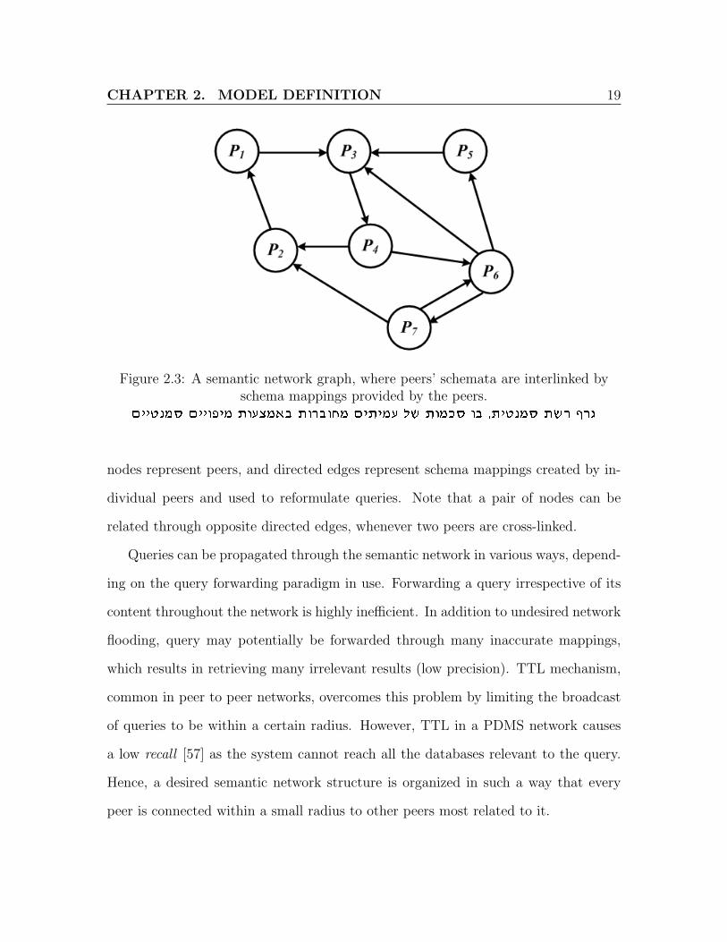
CHAPTER 2. MODEL DEFINITION 19
Figure 2.3: A semantic network graph, where peers’ schemata are interlinked byschema mappings provided by the peers.
miihpnq miietin zervn`a zexaegn mizinr ly zenkq ea ,zihpnq zyx sxb
nodes represent peers, and directed edges represent schema mappings created by in-
dividual peers and used to reformulate queries. Note that a pair of nodes can be
related through opposite directed edges, whenever two peers are cross-linked.
Queries can be propagated through the semantic network in various ways, depend-
ing on the query forwarding paradigm in use. Forwarding a query irrespective of its
content throughout the network is highly inefficient. In addition to undesired network
flooding, query may potentially be forwarded through many inaccurate mappings,
which results in retrieving many irrelevant results (low precision). TTL mechanism,
common in peer to peer networks, overcomes this problem by limiting the broadcast
of queries to be within a certain radius. However, TTL in a PDMS network causes
a low recall [57] as the system cannot reach all the databases relevant to the query.
Hence, a desired semantic network structure is organized in such a way that every
peer is connected within a small radius to other peers most related to it.

CHAPTER 2. MODEL DEFINITION 20
2.2.3 Semantic Topology
Continuing our discussion from Section 2.2.2, consider a semantic network graph
where each peer is mapped against all other peers’ schemata (clique). Potentially,
a query can follow all possible reformulations reaching all peers, thus yielding every
possible answer. However, this architecture does not scale for large networks as query
will flood the network and yield redundant and inaccurate answers. In addition,
matching and mappings maintenance on such a large scale are both time and storage
consuming.
In what follows, we assume a semantic network topology T (P ,M) where every
peer p maintains a list of neighbors N (p), to each member pj of N (p), p maintains a
mappingMSi→Sj. Each peer has a boundary Kp of the number of neighbors according
to its communication and storage capacity. Our network model fits nicely with typical
network models in the context of Peer-to-Peer networks such as power-law networks
[25] and small-world networks [18] that suggest average short path lengths between
peers, and limited number of neighbors distributed according to some power law.
Figure 2.4 presents a visualization of the semantic network separated into layers.
The lowermost layer represents the network topology with links between the peers
representing schemata mappings, limited by fixed number of mappings per peer. The
upper layers represent query translation graphs. Each layer represents a single query
translation between all peers. Query translations and their accuracies (numbers on
the edges) will be discussed in detail in Section 2.3.
The suggested topology can be dynamic. New peers can be discovered by means of
random ping messages as well as through answers to query propagation. By matching
against new peers, peer can expand or replace (if Kp is exceeded) neighbors, thus pos-
sibly improving its ability to obtain answers to queries. In the following we introduce

CHAPTER 2. MODEL DEFINITION 21
Figure 2.4: Semantic Network Model: Query translation layers and a Topology witha limit of Kp = 2 neighbors.
mipkyd xtqn lr ueli` mr dibeletehe zezli`y mebxz zeaky :zihpnqd zyxd lcen
mapping oriented techniques for discovery and replacement of semantic neighbors in
a PDMS setting.
2.3 The Matching Model
The query reformulation mechanism is based on the assumption that the schema
mappings are semantically correct [66, 7], i.e., accurate, which might not be the case
for various reasons. As PDMSs target large scale, decentralized, and heterogeneous
environments where autonomous parties have full control over the design of the local
schemata, it is not always possible to create correct mappings between schemata.
In many situations, an approximate mapping relating two similar but semantically
slightly divergent concepts might be more beneficial than no mapping at all. Also,

CHAPTER 2. MODEL DEFINITION 22
given the vibrant activity in the area of (semi) automatic schemata alignment [24],
we can expect some (most?) of the mappings to be generated automatically in large-
scale settings, with all the associated issues in terms of quality. In this section we
model schema mapping uncertainty and its amplification over transitive mappings
in the context of PDMS query reformulation. We define an estimation measure for
mapping quality, namely matching accuracy, extended to the setting of PDMS where
chained transitive mappings are used, in the form of accuracy preservation.
2.3.1 Mapping Accuracy
As introduced earlier (see Chapter 1), automatic matching may carry with it a degree
of uncertainty, as it is based on syntactic, rather than semantic, means. We intro-
duce the notion of mapping accuracy to characterize the confidence of the mappings
connecting semantically related schemata. We adopt the proposed model of [30], uti-
lizing a fuzzy framework to model the uncertainty of the matching process outcome.
Given a mapping mAi→Ajbetween two attributes, we associate a confidence measure
µm, normalized between 0 and 1, to specify our belief in the mapping quality. We as-
sume that a manual matching is a perfect process, resulting in a crisp matching, with
confidence measure of 1.1 As for automatic matching, a hybrid of algorithms, such
as presented in [20, 38, 27], or adaptation of relevant work in proximity queries (e.g.,
[69, 67]) and query rewriting over mismatched domains (e.g., [44, 43]) can determine
the level of this attribute mapping accuracy estimator.
1This is, obviously, not always the case. In the absence of sufficient background information,human observers are bound to err as well. However, since our methodology is based on comparingmachine-generated mappings with a mapping as conceived by a human expert, and the latter isbased on human interpretation, we keep this assumption.

CHAPTER 2. MODEL DEFINITION 23
Identifying a confidence measure in and of itself is insufficient for matching pur-
poses. One may claim, and justly so, that the use of syntactic means to identify
semantic equivalence may be misleading in that a mapping with a high confidence
measure can be less precise, as conceived by an expert, than a mapping with a lower
confidence measure. In this work, we assume the use of monotonic automatic seman-
tic reconciliation algorithms, where one can safely interpret a resulting mapping with
a high confidence measure as a good semantic mapping. Therefore, high mapping
accuracy suggests (but does not guarantee) a sound mapping that will produce rel-
evant results for queries. Low accuracy on the other hand, implies a mapping with
low confidence level that will most likely produce some irrelevant results.
Suppose we have a schema mapping MSi→Sjfrom pi to pj, composed of a set
of attributes mappings between the corresponding schemata Si and Sj. The schema
mapping confidence measure is a function, a compound confidence measure we calcu-
late using attribute mappings confidence measures. In our work, schema mapping is
computed using average following works such as [29]:
µMSi→Sj=
1
|M|∑
m∈MSi→Sj
µm (2.4)
We calculate query translation accuracy in a similar manner, using average over
the mappings accuracy for attributes participating in the query:
µq(Sj) = µMSi→Sj(q(Si)) =
1
|q|∑
m∈MSi→Sj(q(Si))
µm (2.5)
We use query translation accuracy rather than entire schema mapping accuracy
to evaluate the benefit of peer’s neighbors from a practical point of view, i.e. how
well can it translate queries issued by the peer. To evaluate accuracy over a set of

CHAPTER 2. MODEL DEFINITION 24
queries we use a weighted average using queries appearance frequencies as weights:
µQpi=
1
|Qpi|
∑q∈Qpi
λq ∗ µq (2.6)
Figure 2.5: An example of mapping accuracy.miietin zepekpl dnbec
Example 1 We illustrate the compound mapping accuracy via an example. Assume
a peer p1 is connected to peer p2 and p3 as illustrated in Figure 2.5. Schema mappings
in Figure 2.5 are defined in terms of pairwise directed bipartite graphs whose nodes
represent schema attributes and whose edges represent attribute mappings. Attribute
mapping accuracies are given as edge weights. First, we calculate the schema mapping
accuracies of the matching between p1 and its two neighbors:
µMS1→S2=
1
3∗(µmA1→B2
+ µmB1→A2+ µmC1→C2
)=
1
3∗(0.2 + 0.3 + 0.5) ∼= 0.333 (2.7)
µMS1→S3=
1
3∗
(µmA1→A3
+ µmB1→B3+ µmC1→Null
)=
1
3∗ (0.9 + 0.8 + 0.0) ∼= 0.566
(2.8)
We note that p3 has higher schema mapping accuracy, making it a preferred can-
didate neighbor for p1.
p1 sends a query to its neighbors:
q1(S1) = πA1,B1(S1) (2.9)

CHAPTER 2. MODEL DEFINITION 25
It evaluates as follows against p2 and p3:
q1(S2) = πmA1→B2,mB1→A2
(S2) (2.10)
q1(S3) = πmA1→A3,mB1→B3
(S3) (2.11)
and the corresponding translation accuracies:
µq1(S2) =1
2∗ (µmA1→B2
+ µmB1→A2) =
1
2∗ (0.2 + 0.3) = 0.25 (2.12)
µq1(S3) =1
2∗ (µmA1→A3
+ µmB1→B3) =
1
2∗ (0.9 + 0.8) = 0.85 (2.13)
and the query translations accuracies supporting our assumption for p3 being the pre-
ferred neighbor.
p1 issues another query to its neighbors:
q2(S1) = πC1(S1) (2.14)
evaluating as follows:
q2(S2) = πmC1→C2(S2) (2.15)
q2(S3) = πmC1→Null(S3) (2.16)
with corresponding translation accuracies:
µq2(S2) = µmC1→C2= 0.5 (2.17)
µq2(S3) = µmC1→Null= 0.0 (2.18)
Despite the higher schema mapping accuracy, p3 is least preferred for q2, thus demon-
strating that neighbors preference is query-dependent. Assuming that both q1 and q2
are issued with the same frequency, they have similar weights for p1 and the total
query translation accuracies are:
µQp1 (S2) =1
2∗ (µq1(S2) + µq2(S2)) = 0.375 (2.19)

CHAPTER 2. MODEL DEFINITION 26
µQp1 (S3) =1
2∗ (µq1(S3) + µq2(S3)) = 0.425 (2.20)
Therefore p3 is preferred over p2 considering both queries. Note that for different
weights of query importance, i.e. if q2 was issued much more frequently than q1, the
result might have been opposite and p2 would have been the preferred neighbor.
2.3.2 Mapping Accuracy Preservation
Being a decentralized environment, query reformulation in PDMS relies on the abil-
ity to evaluate transitive mappings among peers’ schemata. When a query is posed
over the schema of a peer, the network will utilize data from any peer that is transi-
tively connected by schema mappings, by chaining mappings. Recall that automatic
semantic matching between two schemata may invlove a degree of uncertainty. For
transitive chained mappings, this uncertainty degree may be amplified due to a com-
position of translations each of which uncertainty affects the accuracy of the following
translations, resulting with mapping accuracy decay.
We introduce the notion of mapping accuracy preservation to characterize the
confidence in a (chained) mappings (transitively) connecting semantically related
schemata. Consider a path of transitively connected peers pi . . . pN composed from a
sequence of schema mappings between the corresponding schemata Si . . . SN :
PathS1→SN= MSN→SN−1
(. . . (MS2→S1)) (2.21)
We associate a confidence measure αPathS1→SN, normalized between 0 and 1, to specify
our belief in the mappings chain quality.
We assume that a chain of mappings resulting from manual matchings will main-
tain the perfect confidence measure of 1, while a chain of mappings that contain
even one most imperfect matching will maintain the lowest confidence measure of 0.

CHAPTER 2. MODEL DEFINITION 27
Further more, we assume the mapping accuracy preservation measure for a chain of
transitive mappings to be bounded by the mapping accuracy of the least accurate di-
rect mapping from below, and that of the most accurate direct mapping from above.
Other two desired characteristics of this confidence measure is commutativity and
monotonicity, i.e. two mapping chains with similar number of mappings and pairs of
mappings with equal accuracy measure will result with equal preservation measure,
and the same scenario with pairs of mappings where mapping from one chain has
higher accuracy measure than the mapping from the other chain for all pairs will
result with a higher preservation measure for the first chain.
The mapping accuracy preservation measure α for a chain of matchings is a func-
tion we calculate using the mapping accuracies of the neighbor schemata in the chain.
Natural suitable candidates for α are functions from the family of triangular norms
(i.e., minimum, product) extended to multiple number of arguments using their as-
sociativity property. We refer the interested reader to [23] for exhaustive treatment
of the triangular norms subject. In our work, chained matchings preservation com-
putation is computed using the product function as the computation operator:
αPathS1→...→SN= αMSN→SN−1
(...(MS2→S1)) =
∏MSi→Sj
∈PathS1→SN
µMSi→Sj(2.22)
Under the monotonicity assumption, high preservation suggests a sequence of sound
mappings, while low preservation implies either a path containing one or more inac-
curate mappings that spoil the entire path accuracy or an accuracy decay along a
chain of non-perfect mappings.
Similarly to schema mappings path, we define a query reformulation path as a
sequence of transitive query translations:
Pathq(SN ) = MSN−1→SN(MSN−2→SN−1
· · · (MS1→S2(q(S1)))) (2.23)

CHAPTER 2. MODEL DEFINITION 28
Query reformulation path preservation is calculated as schema mapping preservation
using the product function over the accuracy measurements of the transitive query
translations:
αPathq(SN )= αMSN−1→SN
(MSN−2→SN−1···(MS1→S2
(q(S1)))) =∏
q(Si)∈Pathq(SN )
µMSi→Si−1(q(Si−1))
(2.24)
Similarly to accuracy measure calculation, we use query translation accuracy rather
than entire schema mapping accuracy. Preservation over a set of queries is calculated
using a weighted average with queries appearance frequencies as weights:
αPathQpi=
1
|Qpi|
∑q∈Qpi
λq ∗ αPathq (2.25)
Figure 2.6: An example of mapping preservation.miietin zepekp xeniyl dnbec
Example 2 We continue with Example 1 above and illustrate the mapping accuracy
preservation calculation. Given the schema mappings depicted in Figure 2.5, assume
an additional connection between p2 and p3 as illustrated in Figure 2.6. First, we

CHAPTER 2. MODEL DEFINITION 29
calculate schema mapping accuracy of the additional matching between p2 and p3:
µMS2→S3=
1
3∗(µmA2→A3
+µmB2→B3+µmC2→Null
) =1
3∗(0.9+0.8+0.0) ∼= 0.566 (2.26)
We can now calculate preservation over the transitive connection of p1 → p2 → p3:
αPathS1→S2→S3= µMS2→S3
∗ µMS1→S2
∼= 0.566 ∗ 0.333 ∼= 0.188 (2.27)
Note that the preservation of direct connection between p1 and p3 equals the accuracy
of this matching:
αPathS1→S3= µMS1→S3
∼= 0.566 (2.28)
and we see that direct matching is preferred over transitive matching. We further
calculate the preservation of q1 through the transitive mappings path. We start with
the transitive translation of q1 from p2 to p3:
q1(S3) = MS2→S3(MS1→S2(q1(S1))) = πmB2→B3,mA2→A3
(S3) (2.29)
and the corresponding query accuracy calculation:
µq1(S3) =1
2∗ (µmB2→B3
+ µmA2→B3) =
1
2∗ (0.9 + 0.8) = 0.85 (2.30)
We can now calculate the query path preservation:
αPathq1(S3)= αMS2→S3
(MS1→S2(q1(S1))) = µMS2→S3
(q1(S2))∗µMS1→S2(q1(S1)) = 0.85∗0.25 ∼= 0.21
(2.31)
As peers perform query reformulations during the propagation process, accuracies
may be calculated on the fly. Calculated accuracies passed along reformulation path
can be used to incrementally calculate accuracy preservation, which in turn can serve
as an indicator in a quality feedback mechanism. We demonstrate such a mechanism
in Example 3.

CHAPTER 2. MODEL DEFINITION 30
Figure 2.7: An example for query reformulation graph.dzli`y ly ly mebxz sxbl dnbec
Example 3 Figure 2.7 shows a query reformulation graph for query q issued by p1.
Directed edges represent query translations from peer to peer, and weights represent
translation accuracies. The dashed line is not part of the query graph, but rather a
virtual mapping, representing the direct translation accuracy of q between p1 and p7,
not known to p1. Peer p1 calculates the translation of q using its mappings to p3 and
propagates the translated query along with its calculated preservation measure:
αPathq(S3)= µMS1→S3
(q(S1)) = 0.8 (2.32)
Peer p3, in turn, further translates q(S3) using its mappings to p4, calculates the accu-
mulated preservation using the received preservation of q(S3) and the newly translated
query accuracy, and propagates the result to p4:
αPathq(S4)= αPathq(S3)
∗ µq(S4) = 0.8 ∗ 1.0 = 0.8 (2.33)
In a similar manner, p4 translates and propagates q(S4) to p7:
αPathq(S7)= αPathq(S4)
∗ µq(S7) = 0.8 ∗ 0.6 = 0.48 (2.34)

CHAPTER 2. MODEL DEFINITION 31
Now note that if p1 and p7 were directly connected, i.e., p1 had matched against p7’s
schema and added it to its neighbors lists, the query translation accuracy preservation
of q from p1 to p7 would have been:
αPathq(S7)= µMS1→S7
(q(S1)) = 0.8 (2.35)
And the direct mapping preservation is higher than the transitive preserved accuracy
calculated. We conclude that p1 is better off with p7 as a neighbor rather than using
the transitive connection through other peers.
In what follows we assume, without loss of generality, that direct matching be-
tween peers is always better, i.e., more accurate, than having connection through
transitive mappings. Hence, peers naturally strive to shortcut mapping paths and
create direct mappings against other peers. Recall that in our model, peers have lim-
ited resources to devote to neighbors maintenance, so acquiring new neighbors may
be at the cost of existing ones. Regardless of any other considerations, peers will be
interested in choosing new neighbors that improve their queries reformulation quality.
2.4 Evaluation of semantic topologies
Considering a dynamic topology where peers periodically update their neighbors,
we need some measures for semantic topology evaluation in the context of mapping
accuracy. We present two approaches for semantic topology evaluation, namely self-
interest based and cooperative-interest based, each representing a topology evaluation
from a different point of view by setting a different “goodness” measure. Using these
measures, we are able to compare different topologies.

CHAPTER 2. MODEL DEFINITION 32
2.4.1 Self-Interest Based Topology Evaluation
Implied by the title, self-interest based topology evaluation represents a measure for
topology quality in the context of mapping accuracy from a single peer narrow point
of view. The basic assumption underlying this approach, is that each peer acts as
an individual according to self centered interest [49]. In the decentralized setting
of PDMS, a peer does not obtain knowledge about other peers’ mappings nor can
it enforce other peers to create mapping links. Under these restrictions, peers may
choose to couple according to their best private knowledge, i.e., by generating a set of
neighbors that maximizes their direct benefit regardless of outside mappings between
other peers.
Let pi be a peer with a set of neighbors Npiand a limit over neighbors number
Kpi. Given a set of queries Qpi
that pi issues, we calculate the peer self-interest value
(SIV ) measure as:
SIVpi=
1
Kpi
∑pj∈Npi
1
|Qpi|
∑q∈Qpi
λq ∗ µq(Sj) (2.36)
We use µq(Sj), measuring the translation accuracy of query q from pi to pj and
multiply by λq representing query importance to pi. We average over all pi’s queries
and get a weighted average of peer’s query set translation accuracy against a single
neighbor pj. We summarize this accuracy over all existing neighbors and divide
(average) by the highest potential neighbors number. Peers connected against as
many peers as they can have and their queries are translated with high accuracy
against their neighbors will receive high SIVpivalue.
Example 4 We demonstrate SIV calculation using the following simple example.
Figure 2.8(a) presents a partial semantic network graph. For ease of presentation,

CHAPTER 2. MODEL DEFINITION 33
Figure 2.8: An example for accuracy oriented semantic topology evaluation.miietin zepekp lr zqqaznd zihpnq dibeleteh zkxrdl dnbec
we consider a single query qp1. Edges’ weights represent semantic query translation
accuracies of qpi. Assuming that pi has a limit of Kpi
= 2 neighbors, Figure 2.8(b)
and 2.8(c) show two semantic topologies for 2.8(a) that are valid under the Kpicon-
straint.
We calculate SIVp1 for the first topology (Figure 2.8(b)) to be:
SIVp1(Tb) =1
2∗ (µqp1 (S3) + µqp1 (S4)) =
1
2∗ (1.0 + 0.9) = 0.95 (2.37)
and similarly, for the second topology (Figure 2.8(c)):
SIVpi(Tc) =
1
2∗ (µqp1 (S3) + µqp1 (S2)) =
1
2∗ (1.0 + 0.8) = 0.9 (2.38)
p1, unaware of the connection between p2 and p4, would prefer the first topology with
N (p1) = {p3, p4} over the second topology with N (p1) = {p3, p2}.
An SIV measure of a topology is calculated by averaging over the peers in the net-
work:
SIVT (P,M) =1
|P|∑p∈P
SIVp (2.39)

CHAPTER 2. MODEL DEFINITION 34
Where T (P ,M) is a semantic topology T with set of peers P and set of query
translation mappings M.
2.4.2 Cooperative Interest Based Topology Evaluation
Cooperative-interest based topology evaluation represents a wider point of view of a
collaborative network of peers trying to achieve global welfare. This approach relies
on the assumption that peers are willing to cooperate in order to achieve a mutually
beneficial topology. Peers may choose to share their knowledge and act in cooperation
to create globally beneficial mappings.
Given a single query q issued by peer pi, we present an evaluation measure that
considers the entire semantic topological structure and calculates the cooperative-
interest value (CIV ) as follows:
CIVqpi= min
pj∈P−pi
{max
Pathq(Sj)∈T (P,M)
{αPathq(Sj)
}}(2.40)
CIV evaluation measure relates to all the semantically connected peers in the topol-
ogy, thus reflecting their ability to form connections in such a way that would benefit
other peers as well. We measure αPathq(Sj), reflecting query translation accuracy to
a (transitively) connected peer. There may be more than a single query translation
path for q from pi to pj in the topology, we evaluate pj’s value by the best translation
path to it and thus we maximize over the paths between pi and pj in the topology.
We then choose the minimal amongst the peers values, representing the worst peer
to answer q under the given topology. Topologies with high preservation for the least
accurate translation path to any peer will receive high CIV .

CHAPTER 2. MODEL DEFINITION 35
Example 5 Continuing our example from Section 2.4.1, we demonstrate CIV cal-
culation over the topologies depicted in Figure 2.8:
CIVqp1(Tb) = min
p2,p3,p4
{αPathq(S2)
, αPathq(S3), αPathq(S1)
}= min {0, 1.0, 0.9} = 0 (2.41)
CIVqp1(Tc) = min
p2,p3,p4
{αPathq(S2)
, αPathq(S3), αPathq(S1)
}= min {0.8, 1.0, 0.8 ∗ 0.1} = 0.8
(2.42)
Unlike the self-interest based evaluation, here the second topology is rated higher then
the first one when using cooperative-based evaluation as q can reach all peers with high
accuracy preservation using this topology.
We calculate CIV measure for a topology as follows:
CIVT (P,M) =1
|P|∑p∈P
1
|Qp|∑q∈Qp
λqp ∗ CIVqp (2.43)
We calculate weighted average over each peer’s query set using query appearance
frequencies as weights reflecting their importance. We then average the values over
all the peers in the network to get the topology value.
Average CIV measure
Although CIV is a good measure for the evaluation of semantic topologies from a
global welfare perspective, it has some insensitivity given bad topologies. Given two
topologies with semantic disconnections (some peers are non-reachable), CIV mea-
sure will associate a 0 value to both and will not be able to distinguish between them.
Therefore, we suggest an alternative CIV measure to be later used for comparison in
our experiments. The average CIV measure, estimates a topology by averaging over
path accuracies rather than by the minimal path accuracy. Formally, the average

CHAPTER 2. MODEL DEFINITION 36
CIV measure is defined as:
CIVT (P,M) =1
|P|∑p∈P
1
|Qp|∑q∈Qp
λqp ∗1
|P − pi|∑
pj∈P−pi
maxPathq(Sj)∈T (P,M)
{αPathq(Sj)
}(2.44)
By averaging over the paths rather than considering the worst (minimal preservation)
path in the topology, we get a measure less sensitive to semantic disconnections.

Chapter 3
On Optimal Semantic Topologies
In Chapter 2 we introduced a model for PDMS, a decentralized network of indepen-
dent peers sharing information through semantic relations, where no peer obtains
complete network structure knowledge. We also presented the influence of the se-
mantic network structure (topology) on the quality of query reformulation. In this
chapter, we assume a centralized setting with complete network knowledge and try
to find optimal semantic topologies. This problem interests us as a baseline for eval-
uating online self organizing topologies. We divide this chapter according to the two
evaluation measures introduced in Chapter 2: in Section 3.1 we present an algorithm
for finding optimal self-interest based topologies, and in Section 3.2 we show that
the problem of finding optimal cooperative-interest based topologies is NP-Complete
even for a very simple case.
37
CHAPTER 3. ON OPTIMAL SEMANTIC TOPOLOGIES 38
3.1 Optimal Self-Interest Based Topologies
Recall that self-interest based topology evaluation is a measurement representing the
selfish nature of peers in the network. It reflects the fact that each peer strives to use
its private knowledge in order to obtain a set of neighbors with the highest possible
schema compatibility. Using the self-interest evaluation measure (SIV ) presented in
Chapter 2, we give a formal representation of the optimal self interest based topology
problem:
Optimal Self Interest Topology Problem
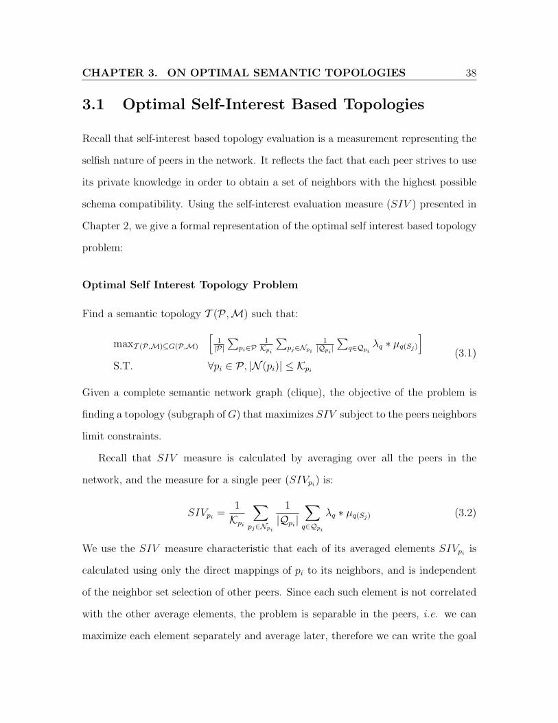
Find a semantic topology T (P ,M) such that:
maxT (P,M)⊆G(P,M)
[1|P|
∑pi∈P
1Kpi
∑pj∈Npi
1|Qpi |
∑q∈Qpi
λq ∗ µq(Sj)
]S.T. ∀pi ∈ P , |N (pi)| ≤ Kpi
(3.1)
Given a complete semantic network graph (clique), the objective of the problem is
finding a topology (subgraph of G) that maximizes SIV subject to the peers neighbors
limit constraints.
Recall that SIV measure is calculated by averaging over all the peers in the
network, and the measure for a single peer (SIVpi) is:
SIVpi=
1
Kpi
∑pj∈Npi
1
|Qpi|
∑q∈Qpi
λq ∗ µq(Sj) (3.2)
We use the SIV measure characteristic that each of its averaged elements SIVpiis
calculated using only the direct mappings of pi to its neighbors, and is independent
of the neighbor set selection of other peers. Since each such element is not correlated
with the other average elements, the problem is separable in the peers, i.e. we can
maximize each element separately and average later, therefore we can write the goal

CHAPTER 3. ON OPTIMAL SEMANTIC TOPOLOGIES 39
function as:
1
|P|∑pi∈P
maxT (P,M)⊆G(P,M)
1
Kpi
∑pj∈Npi
1
|Qpi|
∑q∈Qpi
λq ∗ µq(Sj)
(3.3)
And taking the constants out of the maximization expression we get:
1
|P|∑pi∈P
1
Kpi
∗ 1
|Qpi|∗ maxT (P,M)⊆G(P,M)
∑pj∈Npi
∑q∈Qpi
λq ∗ µq(Sj)
(3.4)
Therefore we can find an optimal self-interest based topology by solving the following
subproblem for each pi ∈ P :
Find a set of neighbors Npisuch that:
maxNpi⊆P
[∑pj∈Npi
∑q∈Qpi
λq ∗ µq(Sj)
]S.T. |N (pi)| ≤ Kpi
(3.5)
Then we can compose links according to resulting neighbor lists for all peers, to get
an optimal self-interest based topology. Following the analysis above we suggest a
formal representation of a simple algorithm for finding such topology.
Algorithm 1 Self-Interest Optimal Topology Algorithm
T (P ,M = {φ})for all pi ∈ P do
for all pj ∈ P , j 6= i doSIVij = 0for all qk ∈ Qpi
doSIVij = SIVij + λqk
∗ µqk(Sj)
sort {pj, j 6= i} by SIVij in a non-ascending orderfor all pj ∈ TOP-Kpi
{SIVij, j 6= i} doM = M∪MS〉→S|
return T (P ,M)
The algorithm starts with a full network graph and an empty topology with all
peers and no mapping links. It then loops over all peers, and for each peer it solves
CHAPTER 3. ON OPTIMAL SEMANTIC TOPOLOGIES 40
the subproblem of finding the neighbors with highest SIV value. This is done by
traversing all other peers (potential neighbors), calculating SIV for each potential
neighbor (lines 5-6), and sorting peers in a non-increasing order of their SIV . Peers
are then added to the topology one by one until reaching the neighbor limit for the
selected peer. The complexity of SIVij calculation is dependent on the size of the
query set of peer pi and the size of the mapping set used for each query qk ∈ Qpi.
This complexity can be calculated for each peer pi as∑
qk∈Qpi|{m|m ∈MSi→Sj
(qk)}|.
Assuming that each attribute A ∈ Spiappears in only a single mapping m ∈MSi→Sj
,
we can set an upper bound to this complexity as follows: |Qpi| ∗ |Spi
| and the total
algorithm complexity is bounded by O(|P|2 ∗maxpi∈P |Qpi| ∗maxpi∈P |Spi
|). For large
networks with many peers, we assume that SIVij calculation is less complex than
looping through all the peers, the overall complexity of the algorithm is bounded by
O(|P|3).
3.2 Optimal Cooperative-Interest Based Topolo-
gies
Recall that cooperative-interest based topology evaluation is a measurement repre-
senting the mutual interest of peers to achieve global welfare. It reflects the fact
that peers are willing to work in collaboration and share knowledge in order to reach
a semantic agreement in the form of topology that maximizes overall queries span
and accuracy potential. Using the cooperative-evaluation measure (CIV ) presented
in Chapter 2, we give a formal representation of the optimal cooperative interest
topology problem:

CHAPTER 3. ON OPTIMAL SEMANTIC TOPOLOGIES 41
Optimal Cooperative Interest Topology Problem
Find a semantic topology T (P ,M) such that:
maxT (P,M)⊆G(P,M)
[1|P|
∑p∈P
1|Qp|
∑q∈Qp
λqp ∗minpj∈P−pi
{maxPathq(Sj)∈T (P,M)
{αPathq(Sj)
}}]S.T. ∀pi ∈ P , |N (pi)| ≤ Kpi
(3.6)
Given a complete semantic network graph (clique), the objective of the problem is
finding a topology (subgraph of G) that maximizes CIV subject to the peers neighbors
limit constraints.
Unlike self-interest based evaluation, the cooperative-interest based evaluation
measure for each peer is highly dependent on the neighbor set selection of other peers.
Other peers selections dictate the available reformulation paths for which cooperative
value elements are calculated. We therefore cannot divide the problem and solve a
subproblem for each peer. In an attempt to solve this problem, we classify it into
several simpler cases as illustrated in Figure 3.1.
Figure 3.1: Classification of the optimal CIV topology problem.CIV jxr z` meniqwnl d`iand dibeleteh z`ivn ziira ly beeiq

CHAPTER 3. ON OPTIMAL SEMANTIC TOPOLOGIES 42
Our primary classification presents the general case where multiple peers issue
queries to the network vs. a simple case where only a single peer issues queries to the
network. Our secondary classification further divides these cases into another two
sub-cases, one where peers issue multiple queries vs. a simpler case where peer(s)
issue a single query only.
The rest of this section is divided as follows: in Section 3.2.1, we introduce the
degree bounded maximum minimal product paths tree (db-MMPT) problem and show
that it is NP-Complete, and in Section 3.2.2 we show using reduction from db-MMPT,
that finding optimal cooperative-interest based topology even for the most simple of
cases, where a single peer issues a single query to the network, is NP-Complete.
3.2.1 Degree Bounded Maximum Minimal Product Paths
Tree (db-MMPT)
We begin with the formal definition of the maximum minimal product paths
tree (MMPT): Given a directed graph G(V, E), with positive edge weights ∀e ∈
E, a(e) > 0, a maximum minimal product paths tree (MMPT) rooted at some node
s ∈ V is a directed subgraph G′(V ′, E ′), where V ′ ⊆ V and E ′ ⊆ E, such that:
1. V ′ is the set of all vertices reachable from s in G,
2. G′ forms a rooted tree with root s, and
3. The minimal weighted product unique simple path from s to any node v ∈ V ′
in G′, is a maximal weighted product path from s to v in G.
Informally, we measure paths in the graph by the product of edge weights and db-
MMPT is a spanning tree of G rooted at s where the worst path (with minimal

CHAPTER 3. ON OPTIMAL SEMANTIC TOPOLOGIES 43
weighted product value) to some arbitrary node v, is the best (with maximal weighted
product value) of all the paths from s to v in the spanned graph G.
We continue with a formal definition of the maximal product paths tree
(MPT): Given a directed graph G(V, E), with positive edge weights ∀e ∈ E, a(e) > 0,
a maximal product path tree (MPT) rooted at some node s ∈ V is a directed subgraph
G′(V ′, E ′), where V ′ ⊆ V and E ′ ⊆ E, such that:
1. V ′ is the set of vertices reachable from s in G,
2. G′ forms a rooted tree with root s, and
3. For all v ∈ V ′, the unique simple path from s to v in G′ is a maximal weighted
product path from s to v in G.
While MPT requires that every path from the root to any node is a maximal
weighted product path in the original graph, MMPT enforces this requirement only
on the path with the least maximum weighted product from the root to any node the
original graph.
Lemma 1 Given a directed graph G(V, E) where all edge weights are positive ∀e ∈
E, a(e) > 0, an MPT rooted at some node s over G is also an MMPT rooted at s
over G.
Proof: Using MPT definition, an MPT rooted at s over G is a tree rooted at s
spanning all the vertices reachable from s in G, and every simple unique path from s
to any node v is a maximum weighted product path in G. In particular, the minimal
weighted product path from s to any node v in the MPT is also a maximal weighted
product path from s to v in G and hence, by the definition of MMPT is also an
MMPT rooted at s over G.

CHAPTER 3. ON OPTIMAL SEMANTIC TOPOLOGIES 44
Figure 3.2: Example for maximum minimal product paths tree (MMPT) andmaximum product paths tree (MPT).
zeilniqwn zeltkn urle zilnipind lelqnd zltkn meniqwn url dnbec
Figure 3.2 shows an example of a graph (part (a)), an MMPT over this graph
(part (b)), and an MPT over this graph (part (c)). We see that the MPT and the
MMPT differ in the path from p1 to p2. However, since the maximal weighted product
path from p1 to p2 is not the minimal of the maximum weighted product paths in
the original graph (the path from p1 to p5 has lower maximum weighted product
path), both trees are MMPTs. Maximal product paths are not necessarily unique
and neither are maximal product paths trees (and hence, maximum minimal product
paths trees).
Next, we present a solution to the problem of finding an MPT over a given graph
G with edge weights 0 ≤ a(e) ≤ 1, using a transformation to shortest paths tree
problem. recall that the formal definition of a shortest path tree is as follows:
Given a graph G(V, E), with positive edge weights ∀e ∈ E, a(e) > 0, a shortest
path tree (SPT) rooted at some node s ∈ V is a directed subgraph G′(V ′, E ′),
where V ′ ⊆ V and E ′ ⊆ E, such that:
1. V ′ is the set of vertices reachable from s in G,

CHAPTER 3. ON OPTIMAL SEMANTIC TOPOLOGIES 45
2. G′ forms a rooted tree with root s, and
3. for all v ∈ V ′, the unique simple path from s to v in G′ is a least sum of weights
path from s to v in G.
The SPT problem of finding a shortest path tree in a given graph as described above
is well researched and can be solved using classical algorithms such as Bellman-Ford
algorithm and Dijkstra’s algorithm [15] with asymptotic complexity of O(|V | · |E|)
and O(|V |2), respectively.
Lemma 2 Given a graph G(V, E) where all edge weights 0 ≤ a(e) ≤ 1, an SPT with
s as a root over the graph G′(V, E) with new edge weights1 a′(e) = log ( 1a(e)
), is an
MPT tree rooted at s over G.
Proof: Let path path1 be a path from s to v in the SPT rooted at s in graph G′ and
an arbitrary path path2 between s and v in G′. From the definition of SPT:
∑e∈path1
a′(e) ≤∑
e∈path2
a′(e) (3.7)
Therefore, ∑e∈path1
log(1
a(e)) ≤
∑e∈path2
log(1
a(e)) (3.8)
Using the well-known equivalence∑
i log xi = log∏
i xi:
log∏
e∈path1
1
a(e)≤ log
∏e∈path2
1
a(e)(3.9)
Since∏
1a(e)
> 0 for any set of edges in G′, and from the monotonicity of the log
function ∏e∈path1
1
a(e)≤
∏e∈path2
1
a(e)(3.10)
1We add a very small value ε to edges with a(e) = 0

CHAPTER 3. ON OPTIMAL SEMANTIC TOPOLOGIES 46
and therefore
1∏e∈path1
1a(e)
≥ 1∏e∈path2
1a(e)
(3.11)
and using the product equivalence 1∏i xi
=∏
i1xi
:
∏e∈path1
a(e) ≥∏
e∈path2
a(e) (3.12)
Since E(G) = E(G′), all the paths in G exits in G′ and vice versa. We have shown
that a path with least weighted sum in G′ is a path with maximal weighted product
in G. Hence, an SPT over G′ is an MPT over G.
Figure 3.3: Example of transformation from MPT to SPT.SPT ziiral MPT ziiran xarnl dnbec
Figure 3.3 shows an example of applying the above suggested transformation from
MPT to SPT. The bold edges on the left hand side graph mark an MPT over the
graph. The right hand side graph is created using log ( 1a(e)
) transformation on the
left graph hand side edges and we see that the SPT over the right hand side graph
(marked again by the bold edges) contains the same edge set as the MPT over the
left hand side graph.
Using the formal definition of MMPT, we continue with the definition of a de-
gree bounded maximum minimal product paths tree (db-MMPT): Given a
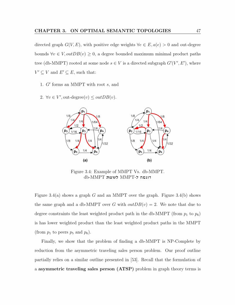
CHAPTER 3. ON OPTIMAL SEMANTIC TOPOLOGIES 47
directed graph G(V, E), with positive edge weights ∀e ∈ E, a(e) > 0 and out-degree
bounds ∀v ∈ V, outDB(v) ≥ 0, a degree bounded maximum minimal product paths
tree (db-MMPT) rooted at some node s ∈ V is a directed subgraph G′(V ′, E ′), where
V ′ ⊆ V and E ′ ⊆ E, such that:
1. G′ forms an MMPT with root s, and
2. ∀v ∈ V ′, out-degree(v) ≤ outDB(v).
Figure 3.4: Example of MMPT Vs. db-MMPT.db-MMPT znerl MMPT-l dnbec
Figure 3.4(a) shows a graph G and an MMPT over the graph. Figure 3.4(b) shows
the same graph and a db-MMPT over G with outDB(v) = 2. We note that due to
degree constraints the least weighted product path in the db-MMPT (from p1 to p6)
is has lower weighted product than the least weighted product paths in the MMPT
(from p1 to peers p5 and p6).
Finally, we show that the problem of finding a db-MMPT is NP-Complete by
reduction from the asymmetric traveling sales person problem. Our proof outline
partially relies on a similar outline presented in [53]. Recall that the formulation of
a asymmetric traveling sales person (ATSP) problem in graph theory terms is

CHAPTER 3. ON OPTIMAL SEMANTIC TOPOLOGIES 48
as follows:
Given a complete directed graph G(V, E), with positive edge weights ∀e ∈ E, a(e) > 0
(where the vertices would represent the cities, the edges would represent the roads,
and the weights would be the cost or traveling distance on that road), find a least
weight Hamiltonian cycle (a round-trip route that visits each city exactly once) over
G.
Theorem 1 Given a directed graph G(V, E), with edge weights 0 ≤ a(e) ≤ 1 and
out-degree bounds ∀v ∈ V, outDB(v) ≥ 0, finding a db-MMPT rooted at some node s
over G is NP-Complete.
Proof: Given an instance of ATSP problem on graph G, we extend and transform
G(V, E) into a new graph G′(V ′E ′) in the following way: we choose an arbitrary node
s ∈ V to be the root. We copy the nodes and edges of G to G′ with new edge weights
a′(e) = 12a(e) . We then extend G′ with a copy of the root, called s′ and a copy of all
the root incoming edges ei,s to ei,s′ such that V ′ = V ∪s′ and E ′ = E∪{ei,s′|ei,s ∈ E}.
The ATSP problem on graph G can then be solved by finding a db-MMPT on graph
G′ with out-degree bounds ∀v ∈ V, outDB(v) = 1. The spanning tree formed by
db-MMPT is a simple path from s to s′, since each node has exactly one successor,
and therefore a Hamiltonian cycle in G (considering s and s′ as one node). We now
show that this simple path in G′ corresponds to a least weight Hamiltonian cycle in
G: Let path path1 be a path from s to s′ in the db-MMPT rooted at s in graph G′
and let path2 be an arbitrary path between s and s′ in G′. From the definition of
db-MMPT: ∏e∈path1
a′(e) ≥∏
e∈path2
a′(e) (3.13)

CHAPTER 3. ON OPTIMAL SEMANTIC TOPOLOGIES 49
Therefore, ∏e∈path1
1
2a(e)≥
∏e∈path2
1
2a(e)(3.14)
and using the product equivalence∏
i1xi
= 1∏i xi
:
1∏e∈path1
2a(e)≥ 1∏
e∈path22a(e)
(3.15)
therefore, ∏e∈path1
2a(e) ≤∏
e∈path2
2a(e) (3.16)
Using the well-known equivalence∏
i axi = a
∑i xi
2∑
e∈path1a(e) ≤ 2
∑e∈path2
a(e) (3.17)
Since∑
a(e) > 0, and from the monotonicity of the power function∑e∈path1
a(e) ≤∑
e∈path2
a(e) (3.18)
and we have shown that the simple path from s to s′ in db-MMPT for G′ is a least
weighted path (Hamiltonian cycle) in G, i.e. this path gives the solution to ATSP in
G. The path is the most restricted form of a (db-MMPT) tree and hence the other
(db-MMPT) trees are generalization of above problem and are harder to solve.
Figure 3.5 shows an example of transformation from ATSP problem to db-MMPT
problem . On the left side, a graph G is presented and a least weight Hamiltonian
cycle over G is drawn (marked by bold edges). On the right, we see the graph G′
resulting from the above suggested transformation of ATSP to db-MMPT. p′4 (marked
bold and shaded) is the extended copy of the selected root p4 in G′, and extended
incoming edges to p′4 are marked by dashed lines. We see that the db-MMPT rooted at
p4 over G′ (marked by bold edges) forms a simple path from p4 to p′4 and corresponds
to the least weighted Hamiltonian cycle in G.

CHAPTER 3. ON OPTIMAL SEMANTIC TOPOLOGIES 50
Figure 3.5: Example of transformation from ATSP to db-MMPT.db-MMPT ziiral ATSP ziiran xarnl dnbec
3.2.2 Single Peer Single Query (SPSQ) Optimal Topology
Problem
Consider the most simple case of Figure 3.1 where only a single peer pi issues a
single query Qpi= {q} to the network while the rest of the peers merely answer and
propagate q. We formalize this problem as follows:
SPSQ Problem
Find a semantic topology T (P ,M) such that:
maxT (P,M)⊆G(P,M)
[minpj∈P−pi
{maxPathq(Sj)∈T (P,M)
{αPathq(Sj)
}}]S.T. ∀pi ∈ P , |N (pi)| ≤ Kpi
(3.19)
Given a complete semantic network graph (clique), the objective of the problem
is finding a topology (subgraph of G) that maximizes CIVqpisubject to the peers
neighbors limit constraints.
Theorem 2 Given a semantic network graph G(P ,M), with associated mapping
accuracies 0 ≤ µM ≤ 1 and neighbor set constraints Kp for each peer p, the SPSQ
problem for a single peer pi with a single query q is NP-Complete.

CHAPTER 3. ON OPTIMAL SEMANTIC TOPOLOGIES 51
Proof: Given an instance of a db-MMPT problem on graph G with edge weights
0 ≤ a(e) ≤ 1 and out-degree bounds ∀v ∈ V, outDB(v) ≥ 0, and some node s ∈ V as
root. We transform the problem to an SPSQ problem as follows: G remains the same
with nodes V taken to be the set of peers P , edges E will be the set of schemata
mappings M, root node s is pi - the single peer issuing the single query q, and edge
weights a(e) are query q translation accuracies µq. The db-MMPT problem on graph
G can then be solved by solving SPSQ problem on G finding some optimal topology
T (P ,M), and then solving MPT on the resulting topology T .
Consider the optimal topology T found by solving SPSQ on G. By the definition
of SPSQ, T spans all the peers connected to pi (all the nodes reachable from s) and
satisfies the neighbor set constraints |N (p)| ≤ Kp,∀p ∈ P (out-degree constraints
out-degree(v) ≤ outDB(v),∀v ∈ V ). Running MPT on T can be done in polynomial
time by transformation to SPT (see Section 3.2.1). By the definition of MPT, the
result of running MPT over T is a tree T ′ spanning all the nodes in T and therefore
spanning all the reachable peers from pi (connected nodes from s) in G. Since T ′
spans a graph that satisfies |N (p)| ≤ Kp,∀p ∈ P (out-degree(v) ≤ outDB(v),∀v ∈ V )
constraints, T ′ satisfies these constraints as well. Let pj (v) be some peer (node)
reachable from pi (s) in G, from the definition of MPT the unique simple path from
pi (s) to pj (v) in T ′ is maximal weighted product path from pi (s) to pj (v) in T , i.e.
the minimum of the maximal weighted product paths in T exists in T ′ and is also
the minimum of the unique simple weighted product paths from pi (s) to any peer pj
(node v) in T ′. By the definition of SPSQ, this path is a maximal weighted product
path from pi (s) to pj (v) in G, hence T ′ is a tree rooted at pi (s) spanning all the
reachable peers (nodes) from pi (s) in G, satisfying G’s neighbors limit (out-degree)
constraints, and the minimum of the weighted product paths from pi (s) to any peer

CHAPTER 3. ON OPTIMAL SEMANTIC TOPOLOGIES 52
pj (node v) in T ′ is a maximal weighted product path from pi (s) to pj (v) in G.
Therefore by the definition of db-MMPT, T ′ is a solution for db-MMPT rooted at s
in G.
Figure 3.6: Example of transformation from db-MMPT to SPSQ.SPSQ ziiral db-MMPT ziiran xarnl dnbec
Figure 3.6 shows an example of a solution to a db-MMPT problem by transfor-
mation to SPSQ problem. On the left side, a graph G is presented with edge weights
0 ≤ a(e) ≤ 1 and out-degree constraints ∀v ∈ V, outDB(v) = 2. For this graph, a
SPSQ optimal topology with p1 as query issuer is presented (marked by bold edges).
On the right side, we see the result of running MPT on this optimal topology (marked
by bold edges). Note that the resulting tree is a db-MMPT rooted at p1 satisfying
the out-degree constraints over the original graph G.
3.3 Discussion
In the search of optimal offline topologies calculation we presented a simple algorithm
that calculates optimal self-interest based topologies in a polynomial time. In addi-
tion, we have shown that even for a very simple case a of single peer issuing a single
query to the network, the problem of finding an optimal cooperative-interest based

CHAPTER 3. ON OPTIMAL SEMANTIC TOPOLOGIES 53
topology is NP-Complete. This problem, named SPSQ, is the most restricted form of
the single peer multiple queries (SPMQ) problems and hence we conclude that
optimal SPMQ topologies are harder to find. Considering the more general problems
of multiple peer single query (MPSQ) and multiple peer multiple queries
(MPMQ) where multiple peers issue queries: under the assumptions that each query
is issued by exactly one peer and no query is equal to or containing another query,
we can show by reduction from SPSQ extended with “virtual” queries that do not
change the optimal topology value, that these problems are also hard.

Chapter 4
Dynamic Self-Organizing
Topologies
In Chapter 2, we presented a model for PDMS and a method to calculate the semantic
accuracy of a query reformulated through a schema mapping. We extended the notion
of semantic accuracy for transitive query translations and presented a method to
calculate accuracy preservation of queries reformulated over a path of peers connected
through schema mappings. We demonstrated how these measures calculation may
be integrated into query translation and propagation mechanism and can serve as
feedback to the quality of the process. In this section, we show how to take advantage
of this feedback to modify the network topology in an automatic manner. Thus,
we make a step towards self-learning networks of peers collaboratively establishing
semantic interoperability in an automated fashion [4].
In the following, we expect peers to perform several tasks: (1) upon propagating a
query, a peer has to calculate the reformulation accuracy and preservation and further
forward these measure along with the new query. (2) upon receiving query results or
54

CHAPTER 4. DYNAMIC SELF-ORGANIZING TOPOLOGIES 55
other feedback (measures), it has to analyze them and update its view of the overall
semantic agreement. (3) Periodically, it has to use its local gained knowledge to
adjust its semantic mappings.
Demonstrated in the Chapter 2, peers can calculate and propagate accuracy mea-
sures along with queries. This light weight mechanism can be extended to pass on
additional informative measures. Forwarding queries with accompanying reformula-
tion measures serves as input for peers to asses semantic similarity. Section 4.1 deals
with semantic similarity assessment in the context of a PDMS. Specifically, we define
the semantic acquaintance problem which is a preliminary phase for filtering suitable
candidates for semantic evaluation. We introduce a methodology and some metrics
for the identification of “good” candidates for matching.
In Section 4.2, we discuss the usage of assessed similarity to perform mapping
adjustments. We introduce the semantic replacement problem which deals with the
practical application of similarity for neighbor list maintenance. If the calculated
similarity measure truly reflects human judgment of similarity, we expect the network
to self-organize into a state where queries get disseminated to the subset of the peers
most likely to return relevant results, where the correct mappings are increasingly
used and where incorrect mappings are neglected. Implicitly, this is a state where a
global agreement on the semantics of the different schemata has been reached.
4.1 Semantic Acquaintance
One of the key conditions for self organizing network establishment is peers ability
to find and connect with new neighbors. Basically, peers can meet other peers using
one of two means: (1) random connection requests through ping messages as part of

CHAPTER 4. DYNAMIC SELF-ORGANIZING TOPOLOGIES 56
the underlying network protocol or (2) acquaintance through queries, i.e., connecting
with peers that produce results to queries issued by the peer.
Upon joining the network, a new peer randomly connects to a set of arbitrary
neighbors. Later on, queries issued by the peer would be reformulated and passed
along to semantically connected peers. However, there may be some peers that are not
included in the group of semantically connected peers, yet still capable of answering
peers queries.
Figure 4.1: Semantically disconnected components.mixiyw izla miihpnq miaikx
Example 6 Consider the network in Figure 4.1, representing a partial semantic
translation network for query q issued by peer p1. Peer p1 joined the network and
established connection with N (p1) = {p2, p3}, the dashed edge is a virtual connection,
non-existing in the network, demonstrating the potential mapping MS1→S5.
The only connection between the peers in the left side of the graph (p1, p2, p3)
and those on the right side of the graph (p4, p5, p6, p7) is by the mapping MS3→S4.
Unfortunately, q cannot be reformulated over this mapping (µq = 0), maybe due to

CHAPTER 4. DYNAMIC SELF-ORGANIZING TOPOLOGIES 57
some missing attributes in p4’s schema, and therefore query q will not reach the peers
on the right side. If there was an actual connection MS1→S4, the query q could have
been reformulated over this mapping and further propagated to other peers as well.
In the absence of a central mechanism to identify semantically disconnected compo-
nents in the network, it is up to each peer to try and bridge over such disconnections
and expand its semantic connected component. Imitating the procedure performed
when joining the network, peers can periodically match against random peers that
they are not familiar with, i.e., peers that never answer its queries.
Assuming a well connected topology, semantic disconnections will not be that
common. Peers can therefore focus on selecting preferred neighbors among the tran-
sitively connected peers discovered during query propagation. Neighbors are chosen
according to their semantic similarity to the selecting peer, reflecting their ability to
translate its queries. Schema matching is the basic operation used to asses semantic
similarity in our model.
Schema matching is a complex [14] time-consuming operation. In [30], it is demon-
strated through empirical analysis that there is no single dominant schema matcher
that performs best, regardless of the data model and application domain. Therefore,
more complex and time-consuming approaches such as matchers ensemble [19, 29] and
top-ranked matchings evaluation [28] are required to establish correct mappings, and
there is no evidence that these approaches can reach a “consensus” of valid schema
matching at a low complexity cost [22].
Recall that the main objective of peers in a PDMS is to share knowledge by means
of queries and therefore the effort dedicated for examination of potential neighbors
should be minimal. The process of finding new neighbors should be light-weight,
complexity wise, for it to scale under such settings where peers perform the process

CHAPTER 4. DYNAMIC SELF-ORGANIZING TOPOLOGIES 58
frequently.
We present the concept of semantic acquaintance to address this problem, se-
mantic acquaintance involves the selection of “good” candidates for schema matching
among the peers discovered through a query mechanism. The idea behind semantic
acquaintance is to apply light-weight decision policies to narrow the list of potential
candidates to include only peers anticipated to have high semantic similarity. Ac-
quaintance policies can make use of measures returned as feedback from the query
mechanism. Light weight acquaintance policies, such as least recently used (LRU)
[62], History, and Popularity [68] to name a few, were formerly suggested and proved
effective in the context of file sharing P2P networks. However, file sharing networks
are different from PDMS in several respects. Firstly, a query answer is given in the
form of yes/no for the existence of a desired file, and a positive reply from a single
source is sufficient. In addition, the context of matching links with their accompany-
ing accuracies does not exist in file-sharing systems. Therefore, despite the fact that
mechanisms from file sharing networks can be generalized and used in the context of
PDMS, accuracy preservation oriented policies may better fit our setting.
In what follows, we introduce several acquaintance policies taking into account
the special characteristics of PDMSs:
Highest Path Length Acquaintance (HPLa) Policy
Highest path length policy takes into account the decay of path accuracy along a
path of transitive mappings. The longer the path is, the higher are the chances for
accuracy decay. For this policy, peers have to forward along with reformulated query
the measure δPath, counting the number of query translations along a path. This
measure is easily calculated as each peer translating a query increases its value and

CHAPTER 4. DYNAMIC SELF-ORGANIZING TOPOLOGIES 59
further forwards it, and formally:
HPLa(pj, q) = δPathpi→...→pj(4.1)
Highest Accuracy Preservation Acquaintance (HAPa) Policy
Highest Accuracy Preservation policy follows the principle of “a friend of a friend,
is also a friend,” which means under PDMS setting that a well matched neighbor
of a well matched neighbor is a good candidate for matching and more generally,
transitively connected peers that maintain high preservation mappings paths are likely
to match a peer with high accuracy. This policy requires the propagation of the path
preservation measure αPath as demonstrated in Chapter 2, and formally:
HAPa(pj, q) = αMSl→Sj···(MSi→Sk
(q)) (4.2)
Nearest Neighbors Accuracy Acquaintance (NNAa) Policy
Nearest neighbors accuracy policy tries to take advantage of both semantic connec-
tivity and connections quality of peers. Assuming that a peer is well connected to
other peers, matching against it would earn the benefit of queries reaching its neigh-
bors. In this policy, each peer summarizes the accuracy of its closest neighbors and
returns this measure along with query results. Note that this form of measure can
have a simple form of nearest neighbors accuracy for a given schema/query relevant
for the receiving peer or generalized form so that nearest neighbors in a given radius
(number of hops). The latter requires a cooperative calculation protocol. We define
it formally as:
NNAa(pj, q) =∑
pk∈N (pj),k 6=i
µMSj→Sk(q) (4.3)

CHAPTER 4. DYNAMIC SELF-ORGANIZING TOPOLOGIES 60
Figure 4.2: Acquaintance policies example.zexkd zeieipicnl dnbec
Example 7 We demonstrate the application of the above policies in the following
example. Figure 4.2 presents a partial network of semantically connected peers. Num-
bers on the edges represent the translations accuracies of query q, issued by peer p1.
Assume that q reaches the peers in the following order p3, p4, p2, p6, p7, p5 and that dur-
ing a single query session, peers answer only the first time the query reaches them,
i.e., p2 will answer q upon receiving it from p4 and will not answer it upon receiving
it the second time from p7.
We demonstrate now the calculation of candidate peers evaluation measures ac-
cording to the policies introduced in this section for peer p4:
HPLa(p4, q) = δPathp1→p3→p4= 2 (4.4)
HAPa(p4, q) = αMS3→S4(MS1→S3
(q)) = 0.8 ∗ 1.0 = 0.8 (4.5)
NNAa(p4, q) =∑
pj∈N (p4),j 6=1
µMS4→Sj(q) = µMS4→S2
(q) + µMS4→S6(q) = 0.8 + 0.9 = 1.7
(4.6)
In a similar manner, we calculated these measures for the rest of the peers. The

CHAPTER 4. DYNAMIC SELF-ORGANIZING TOPOLOGIES 61
pj p4 p2 p6 p7 p5
HPLa(pj, q) 2 3 3 4 4HAPa(pj, q) 0.8 0.64 0.72 0.72 0.648NNAa(pj, q) 1.7 0.7 1.8 0.9 0.6
Table 4.1: Acquaintance policies evaluation measureszexkd zeieipicn zkxrd iccn
results are summarized in the Table 4.1:
Note that different policies may yield different rankings: p5 and p7 are ranked first
according to HPLa policy, p4 according to HAPa policy, and p6 according to NNAa
Policy. While HPLa policy explicitly prioritizes longer paths, HAPa implicitly prefers
shorter ones, where preservation is often maintained higher. NNAa policy, completely
ignores path length.
4.2 Semantic Replacement
In Section 4.1 we presented some policies for identification of semantic similar peers.
However, considering the decentralized setting and the absence of complete network
knowledge, none of the suggested (or any other) policies guarantee a selection of good
candidates for matching, they merely offer a lightweight heuristics to avoid exhaustive
matchings. Further more, even a selected candidate with high matching accuracy will
not necessarily be a good neighbor. Neighbors can be matched well and still translate
some queries inaccurately thus spoiling the peer’s self-interest. Others may offer
accurate translation but are not well connected to other peers thus possibly spoiling
the global welfare as queries may not reach many peers through them. We illustrate
these problems in the following example:

CHAPTER 4. DYNAMIC SELF-ORGANIZING TOPOLOGIES 62
Example 8 Consider Example 7, presented in Section 4.1. Figure 4.2 presents the
network graph and Table 4.1 summarizes the results of applying HPLa, HAPa and
NNAa acquaintance policies on the peers discovered through query process of q issued
by p1. Assume now that p1, applying all the three policies, decides to match against
the top ranked peer of each policy,1 the matching accuracies are given in Table 4.2:
HPLa HAPa NNAa
pj p7 p5 p4 p6
µMS1→Sj(q) 1.0 0.9 0.92 0.95
Table 4.2: Mapping accuracies for selected candidates using different acquaintancepolicies
zepey zexkd zeieipicn it lr mixgap mizinrl ietin zepekp
Assume now that p1 has a limit of Kp1 = 1 neighbors. Comparing the matching
results of all four peers, p1 discovers that p7 has highest accuracy and has in fact, a
perfect mapping. Since µMS1→S7(q) > µMS1→S3
(q), p1 decides that p7 is a better neighbor
than p3 and makes a replacement. The new topology after the replacement is given
in Figure 4.3: In the new topology, p1 achieved a (possibly) better mapping with p7,
but at the cost of loosing good mapping connections to four other peers (circled by a
dashed line). Surely, the replacement of p3 with p7 is not a good option. Replacement
with any of the other candidate peers would not have spoiled the connectivity and thus
could be considered.
Example 8 demonstrates the need for a replacement policy. Replacement deals
with the maintenance of a valuable neighbor list, by providing the decision policy for
acceptance or rejection of new peers to the list. We examine the simple event of a
single replacement candidate, where multiple candidates events can be separated into
1In this example, we consider both HPLa policy yielded top ranked peers (p7, p5)

CHAPTER 4. DYNAMIC SELF-ORGANIZING TOPOLOGIES 63
Figure 4.3: Bad replacement example.dtlgd zeieipicnl dnbec
a sequence of discrete events, each dealing with a single candidate. As each peer is
limited to a finite number of allowed neighbors, there may be two possible decision
scenarios: (1) there exists an open slot in the list, the replacement policy becomes
a placement policy and the new candidate is added to the list or (2) the list is full
and any placement exceeds the neighbors limit. Here, a replacement policy needs
to decide whether to accept new candidate to the list, and at the expense of which
existing neighbor.
Acquaintance and replacement can be viewed as two parts of a problem of identifi-
cation and maintenance of semantic neighbors. Acquaintance and replacement polices
can be coupled to run serially as a single global policy, and in some cases, a single
policy can fit for both. In what follows, we introduce a few examples for acquain-
tance complementary policies that may serve for neighbors replacement decisions in
a PDMS:

CHAPTER 4. DYNAMIC SELF-ORGANIZING TOPOLOGIES 64
Highest Accuracy Preservation Replacement (HAPr) Policy
Highest accuracy replacement policy ranks neighbors according to their schema match-
ing accuracy or query set translation accuracy. This policy is actually similar to HAPa
acquaintance policy, where preservation for directly connected neighbors is calculated
as their matching accuracy. HAPr is a self-interest based oriented replacement policy,
as it guarantees that each replacement does not spoil the closest neighbors accuracy
of the peer. We calculate HAPr as:
HAPr(pj) =∑
q∈Qpi
λq ∗ µq(Sj) (4.7)
Nearest Neighbors Accuracy Replacement (NNAr) Policy
This policy is a good example of a policy that can serve both for acquaintance and
replacement, following the same principle of connecting with neighbors with high total
mappings accuracy. We can either add the matching accuracy of the new candidate
to the sum of its nearest neighbors accuracies, or we can multiply it with the sum to
calculate the nearest neighbors accuracy preservation. We use the second option:
NNAr(pj) =∑
q∈Qpi
λq ∗
µq(Sj) +∑
pk∈N (pj),k 6=i
αMSj→Sk(MSi→Sj
(q))
=
∑q∈Qpi
λq ∗ µq(Sj) ∗
1 +∑
pk∈N (pj),k 6=i
µq(sk)
(4.8)
Near Highest Accuracy Preservation Replacement (HAP80%r) Policy
This replacement policy is a variation on the HAPr policy and calculated in the same
manner, but the acceptance rule is different. Rather than replacing the least accurate
neighbor with a new candidate only if the new peer has higher HAP value, we enforce

CHAPTER 4. DYNAMIC SELF-ORGANIZING TOPOLOGIES 65
the replacement even if the new peer has higher value than 80% of the least accurate
neighbor. Since HAPr is a self-interest based policy, this weak form of HAPr accepts
neighbors that may contribute for the network cooperative-interest value and still not
spoil much of the self-interest value of the network.
Example 9 We continue with Examples 7 and 8 and demonstrate the outcome of
applying the above suggested replacement policies on the network in Figure 4.2. First,
we calculate the different replacement measures for the current neighbor p3, in order
to compare it with the new candidates.
HAPr(p3) = µq(S3) = 0.8 (4.9)
HAP80%r(p3) = 0.8 ∗ µq(S3) = 0.8 ∗ 0.8 = 0.64; (4.10)
NNAr(p3) = µq(S3) ∗ (1 + µq(S4)) = 0.8 ∗ (1 + 1) = 1.6; (4.11)
Similarly, we calculate HAPr and NNAr measures for the different acquaintance
policies top-ranked peers, as detailed in Table 4.2. The results are given in Table 4.3:
HPLa HAPa NNAa
pj p7 p5 p4 p6
HAPr 1.0 0.9 0.92 0.95NNAr 1.9 1.44 2.484 2.755
Table 4.3: Replacement policies evaluation measuresdtlgd zeieipicn zkxrd iccn
According to all the suggested policies, p3 would be replaced by any of the peer
candidates. We get that NNAr replacment policy top ranked p6, retrieved by NNAa
acquaintance policy, while HAPr replacement policy top ranked p7, retrieved by HPLa

CHAPTER 4. DYNAMIC SELF-ORGANIZING TOPOLOGIES 66
acquaintance policy. As we saw in Example 8, replacement of p3 with p7 is a bad
option although it improves the self-interest value of p1 as it disconnects a group of
other peers that become non-reachable. As for p6, we compute CIV before and after
the replacement, as follows:
CIVpre = min{max{0.8 ∗ 1 ∗ 0.8, 0.8 ∗ 1 ∗ 0.9 ∗ 1 ∗ 0.9},
0.8, 1 ∗ 0.8,
0.8 ∗ 1 ∗ 0.9 ∗ 0.9,
0.8 ∗ 1 ∗ 0.9,
0.8 ∗ 1 ∗ 0.9 ∗ 1} = 0.576
(4.12)
CIVpost = min{max{0.95 ∗ 1 ∗ 0.9, 0.95 ∗ 0.6 ∗ 1 ∗ 0.8, 0.95 ∗ 0.9 ∗ 0.6 ∗ 1 ∗ 0.8},
max{0.95 ∗ 0.6, 0.95 ∗ 0.9 ∗ 0.6},
max{0.95 ∗ 0.6 ∗ 1, 0.95 ∗ 0.9 ∗ 0.6 ∗ 1},
0.95,
0.95 ∗ 1} = 0.57
(4.13)
We see that the replacement of p3 with p6 improves the self-interest value, yet spoils
the cooperative-interest value. However, CIV is only slightly decreased so this option
may be considered to be a good one.
In Chapter 5 we simulate a PDMS network and evaluate our different acquaintance
and replacement policies performance.

Chapter 5
Experiments
In this chapter we describe simulation of a PDMS implemented according to our
model. We run experiments using various combinations of acquaintance and replace-
ment algorithms and compare their results. This chapter is divided as follows: Sec-
tion 5.1 describes the simulation architecture. Next, in Section 5.2 we give details
on different data and parameters used in our simulation and the methods we used to
generate them. Then, in Section 5.3 we present the setup for our experiments. In
section 5.4 we detail the measures used to evaluate our results. Section 5.5 summa-
rizes the results of our experiments and finally, in Section 5.6 we give provide a brief
discussion and main conclusions regarding our results.
5.1 Simulation Architecture
Figure 5.1 illustrates our simulation architecture. We now provide a detailed descrip-
tion of its components.
67

CHAPTER 5. EXPERIMENTS 68
Figure 5.1: Simulation Model: domain, schemata, and query sets.zezli`y itqe`e zenkq ,mibyen mler :divleniqd lcen
Configuration: The input of the simulation is a configuration file, allowing us
to control the distributions parameters, the number of domains and peers, sizes of
average query set and query and additional simulation parameters.
Domains: Domains are a representation of the set of concepts existing in the world.
We generate an assortment of elements representing available concepts. In this chap-
ter, we run experiments with single a domain.
Schemata: A schema is a set of elements representing peer’s knowledge base as
exposed to other peers. Schemata are composed of a selection of elements from a
single or multiple semantic domains.
Queries: Each peer is assigned with a set of queries it issues to the network. Queries
are generated using elements from peers’ schemata.

CHAPTER 5. EXPERIMENTS 69
Schema mappings: A schema mapping is composed of a set of element mappings
and their associated accuracies. We generate mappings between all element pairs in
source and target schemata, and then calculate maximum accuracy matches between
the schemata.
Query translation: A query translation represents a query reformulation from a
source peer schema to a target peer schema. Using schema mappings, we generate
query translations between all peers and calculate their corresponding accuracies.
Query translations supply the accuracies (edge weights) for the semantic matchings
layer of the network.
Topology: A topology represents the semantic network layer of the system. Spec-
ifying neighbors list for each peer, topology simulates the semantic connections be-
tween the peers. Topology spans a partial network (subgraph) of a fully connected
network (clique) that follows the neighbors number (out-degree) limitation for each
peer. Queries are executed over an initial topology and their results are analyzed
and used to adjust these topologies, according to the various policies discussed in this
thesis.
Query sequence generator: A query sequence generator generates a sequence of
pairs (peer, query), representing a serialization of parallel queries issued by peers in
the network. A generated sequence will be used to run queries in a given order for a
variety of different settings.

CHAPTER 5. EXPERIMENTS 70
Figure 5.2: Simulation Model: semantic topology and query translation layers.zezli`y mebxz zeakye zihpnq dibeleteh :divleniqd lcen
Query process generator: A query process generator takes a given pair (peer,
query) and a topology, and generates a query process over this topology using proba-
bilistic hop count mechanism to limit query span. Query process uses corresponding
query translation to calculate preservation along query paths. Query process results
in a list of non-neighbor candidate peers with their corresponding query measures
such as path length, path preservation, etc.
Acquaintance algorithm: An acquaintance algorithm takes a list of potential
candidate neighbors and ranks them according to some acquaintance policy. Top-
ranked peers are selected as candidates for replacement.

CHAPTER 5. EXPERIMENTS 71
Replacement algorithm: A replacement algorithm takes a candidate peer and a
list of neighbors and evaluates them according to some replacement policy. Replace-
ment algorithm may modify a given topology by replacing a link from an existing
neighbor to a new one.
Figure 5.3: Simulation Model: sequence Diagram of a single query cycle.dcigi dzli`y xear zelert svx miyxz :divleniqd lcen
Figure 5.3 presents a sequence diagram for a single query cycle: first, a single peer
issues a single query to the network. Query process results in a list of non-neighbor
peers and their associated measurements, required for acquaintance and replacement
algorithms. On the selected candidate, we run an acquaintance algorithm to identify
the best matching candidate. We then run a replacement algorithm with the selected
candidate peer and the list of the query issuer neighbors, and adjust the current
topology according to the algorithm decision.

CHAPTER 5. EXPERIMENTS 72
5.2 Data and parameters
General configuration: Table 5.1 summarizes a set of fixed simulation parameters:
Parameter ValueNumber of Domains 1Attributes per domain 20Number of Peers 25Maximum queries per peer 3
Table 5.1: Simulation parametersdivleniql mixhnxt
Attributes and queries distribution: we model domain attribute distribution
over peers using Zipf distribution. We rank attributes and then generate attributes for
each peer separately using this ranking and Zipf(4,1). We define a maximal number of
queries per peer and assume a uniform distribution Uniform(1,MaxQueries) for peers
query set size. For each query we assume attributes participation using their rank
and Zipf(2,0.75) over peers attributes. Figure 5.4 shows the probability of attributes
to be selected for a schema and a single query of a single peer according to their
rank. We assume this model so that most peers share similar attributes and thus can
translate queries, while some attributes are more rare and can be translated only over
several semantically related peers. Selection of Zipf distribution parameters were set
according to the number of attributes in the domain such that the average schema
size is 11 and the the average query size is 6.
Schema matchings: we generate attribute matching accuracies using two normal
distributions: correct attributes matching accuracies are distributed N(0.8,0.2), and
wrong attributes matching accuracies are distributed N(0.2,0.2). Both distributions

CHAPTER 5. EXPERIMENTS 73
Figure 5.4: Domain attributes probability for participation in peer schemas andqueries.
zyxa mixagd ly zenkqa mibyen zellkidl zexazqd
are trimmed at 1 where all accuracies above are set to 1 (perfect match), and at
0 where all accuracies below 0 are set to 0 (worst match). Figure 5.5 presents the
two distributions graphically. We generate schema mappings by constructing a bipar-
tite graph with source schema attributes and target schema attributes as nodes and
generated attribute matching accuracies as edge weights. We calculate 1:1 matching
between two schemata by running Abest maximum weighted bipartite graph algorithm
[41] over the constructed graph, the result of such matching is a set of attribute map-
pings. Using these mapping sets and the previously generated accuracies, we calculate
query translation accuracies.
Topologies we assume network topology to follow power law rules, similar to struc-
tures discovered on research of Internet topology [25]. We use power-law out degree
(PLOD) generator [54] to generate initial network topologies. Figure 5.6 presents
peers out degree according to their rank and the corresponding log-log chart for a 25
peers network. The highest ranked peer is connected to about half of the network

CHAPTER 5. EXPERIMENTS 74
Figure 5.5: Attributes mapping accuracies distributions for similar and differentattributes.
mipeye midf mibyen xear zezli`yd zepekp zeiebltzd
and the lowest ranked peer is connected to a single neighbor. The log-log chart shows
that the topology follows desired power-law characteristic.
Figure 5.6: Network topology: out degree Vs. peer rank following power law.power law zeiweg zniiwn bexic lenl d`ivi zbxc :zyxd ziibeleteh
Simulation sequences: we generate random query sequences using Uniform(1,peersNumber)
distribution to select query issuers and Uniform(1,peerQueries) distribution to select
issued queries. We repeat the process until we reach the desired sequence size.

CHAPTER 5. EXPERIMENTS 75
5.3 Experimental setup
We implemented six acquaintance policies. The first two are LRUa and Historya,
taken from the context of file-sharing peer-to-peer systems [62, 68]. The next three are
our suggested HPLa, HAPa, and NNAa policies. Last, we implemented Randoma
policy for a baseline comparison. Additionally, we implemented six replacement poli-
cies. The first two, LRUr and Historyr matching the similar acquaintance policies.
Next are our three policies of HAPr, HAP80%r and NNAr. Once again we impele-
mented Randomr policy to be used as a baseline. We implemented our simulation
using Java 2 JDK version 1.4.2 environment, and ran experiments on a laptop with
Intel Centrino Dual core T2300 1.66GHz CPU, 1GB of RAM and Windows XP Pro-
fessional OS.
Parameter ValueMatching configurations 10Initial topologies 10Query sequences 10Queries per sequence 5000
Table 5.2: Summary of experimental setup parametersdivleniqd zvixl mixhnxt ly mekiq
As described in Table 5.2, we generate initial sets of: ten matching configurations,
ten initial topologies, and ten query sequences. We run experiments, each using a
different combination of matching configuration, initial topology, and query sequence,
selected from the corresponding generated sets. In the rest of this chapter, given
results are calculated using an average over the results of different experiments. We
divide our experiments according to the following three settings:

CHAPTER 5. EXPERIMENTS 76
• “Good” topologies1: we generate initial optimal semantic topologies and apply
different policies for their reorganization.
• “Bad” topologies: we generate initial far from optimal semantic topologies and
apply different policies for their reorganization.
• Random topologies: we generate random semantic topologies and apply differ-
ent policies for their reorganization.
The first two settings serve for sanity checks, enabling us to examine the sensitivity
of different policies and evaluation metrics to extreme situations. In the last setting,
we examine the effect of applying different policies on “average” random generated
topologies.
Under each setting, we make the following two type of experiments:
• Acquaintance policies comparison using a fixed replacement policy.
• replacement policies comparison using a fixed acquaintance policy.
5.4 Evaluation
In our experiments we evaluate acquaintance and replacement policies using the fol-
lowing metrics:
Convergence: We measure convergence in terms of steps, i.e., the number of
queries after which there is no change in the topology. Formally, we say that a
1We generate “good” and “bad” topologies by setting high and low query translation accuraciesbetween source and target peers. We use N(0.9,0.05) distribution for high translation accuracies,and N(0.1,0.05) distribution for low translation accuracies, both distributions trimmed at 0 frombelow and at 1 from above. Good neighbors will be associated with high translation accuracies andbad neighbors will be associated with low translation accuracies

CHAPTER 5. EXPERIMENTS 77
policy converges at step t− d if for some (threshold) number of queries d, t ≥ d
T (P ,M)t = T (P ,M)t−1 = · · · = T (P ,M)t−d (5.1)
Topology changes: We measure effective topology changes performed by a policy.
Formally, given an initial topology T (P ,M)0 and n issued queries, we calculate
topology changes as: ∑t=1...n
I{T (P,M)t 6=T (P,M)t−1} (5.2)
SIV change: We measure the effect of applying policies on the semantic topology
self-interest improvement in terms of change in the SIV measure. Formally, given an
initial topology T (P ,M)0 and n issued queries, we calculate SIV change as:
∆SIV =SIVT (P,M)n
− SIVT (P,M)0
SIVT (P,M)0
(5.3)
CIV change: We measure the effect of applying policies on the semantic topology
global welfare improvement in terms of change in the CIV measure. Formally, given
an initial topology T (P ,M)0 and n issued queries, we calculate CIV change as:
∆CIV =CIVT (P,M)n
− CIVT (P,M)0
CIVT (P,M)0
(5.4)
Reachability: We also measure the effect of our policies on the network structure
in the form of changes in the in-degree of peers, reflecting the reachability of peers.
Formally, given an initial topology T (P ,M)0 and n issued queries, we calculate the
change in each in-degree level 0 ≤ i ≤ |P − 1| as:
∆in-degree(i) =∑
p∈T (P,M)n
I{in-degree(p)=i} −∑
p∈T (P,M)0
I{in-degree(p)=i} (5.5)

CHAPTER 5. EXPERIMENTS 78
5.5 Results
In this section we present the outcome of our experiments, divided into three subsec-
tions according to the settings described in Section 5.3: Section 5.5.1 describes our
results given good initial topologies, in Section 5.5.2 we detail our results given bad
initial topologies, and in Section 5.5.3 we give our results using randomly generated
topologies.
5.5.1 Good Initial Topologies
We have created a set of optimal topologies where each peer maintains high mapping
accuracy with its initial neighbors and low mapping accuracy with all the other peers.
In addition, we made sure that all query translations from peers that do not issue
them, maintain low translation accuracies. By that, we created a topology where each
peer is connected to a neighbor set best for it, and the transitive connection to other
peers is less relevant (since its associated accuracy is low), and hence, there is no mo-
tivation for peers to change their neighbors. We calculated the average measurements
for our good initial topologies and the results are given as follows: SIV measure value
is 0.899556702 close to the average generated mapping accuracy between good neigh-
bors (0.9). CIV measure value is 0.000113392, reflecting preservations of worst query
translation paths, and average CIV measure value is 0.141919149, higher then CIV
since it averages rather than minimizes preservation over query translation paths.
Acquaintance Policies Comparison
We have tested the different acquaintance policies using fixed HAPr replacement
given a good initial topology and our results indicate that there were no changes in

CHAPTER 5. EXPERIMENTS 79
the topologies and the metrics were not updated. These results fit our setting of
initial optimal topologies.
Replacement Policies Comparison
We present a comparison between different replacement policies using fixed HAPa
acquaintance given a good initial topology. We get similar results using other fixed
acquaintance policies.
Figure 5.7: Replacement policies comparison: convergence in initial good topologieszeaeh zeizlgzd zeibeleteh ozpda zeqpkzd :dtlgd zeieipicn z`eeyd
Convergence: Figure 5.7 shows the convergence of different replacement policies
given a good initial topology. LRU and History policies, replacing only peers that
do not translate queries, converge at 0 since all the initial neighbors translate all the
queries. HAP and HAP80% policies, replacing peers with low SIV , converge at 0
since the all non-neighbors maintain lower SIV than any neighbor. Random, making
coincidental replacements, does not converge, and therefore is not shown in the graph.
NNA policy converges after 428 steps. Recall that NNA measures peers according
to their neighbors accuracy sum, so that peers with larger number of neighbors than

CHAPTER 5. EXPERIMENTS 80
others may be ranked higher, causing NNA to make wrong replacement decisions in
this case of an initial optimal topology.
Figure 5.8: Replacement policies comparison: topology changes in initial goodtopologies
zeaeh zeizlgzd zeibeleteh ozpda dibeleteh iiepiy :dtlgd zeieipicn z`eeyd
Topology changes: Figure 5.8 shows the numbers of topology changes each policy
makes given a good initial topology. Figure 5.8 (left) shows that Random policy,
making coincidental replacements, performs (wrong) changes in 20% of the queries.
LRU, History, HAP and HAP%80 preform no changes (converging after 0 steps).
Figure 5.8 (right) shows the same data excluding Random policy and we can see that
NNA policy performs changes in about 0.06% of the queries only.
SIV change: Figure 5.9 shows SIV change for each policy given a good initial
topology. Random policy, making many wrong replacements, spoils SIV by 74%.
LRU, History, HAP, and HAP80% policies, making no topology changes, do not
change SIV . NNA policy, making around 3 wrong replacements, spoils SIV by 3%.
These results fit well with the topology being a SIV optimal topology where each
change can only spoil SIV .

CHAPTER 5. EXPERIMENTS 81
Figure 5.9: Replacement policies comparison: SIV change in initial good topologieszeaeh zeizlgzd zeibeleteh ozpda SIV ikxra iepiy :dtlgd zeieipicn z`eeyd
Figure 5.10: Replacement policies comparison: CIV change in initial good topologieszeaeh zeizlgzd zeibeleteh ozpda CIV ikxra iepiy :dtlgd zeieipicn z`eeyd

CHAPTER 5. EXPERIMENTS 82
CIV change: Figure 5.10 shows CIV change for each policy given a good initial
topology. Random policy, making many wrong replacements, spoils CIV by 58%.
LRU, History, HAP, and HAP80% policies, making no topology changes, do not
change CIV . NNA policy, making around 3 wrong replacements, spoils CIV by 5%.
These results fit well will the topology being a CIV optimal topology where each
change will spoil CIV .
5.5.2 Initial Bad Topologies
We have created a set of far from optimal topologies where each peer maintains low
mapping accuracy with its initial neighbors and high mapping accuracy with some
other non-neighbor peers. In addition, we made sure that all query translations from
peers that do not issue them, maintain low translation accuracies. By that, we created
a topology where each peer is connected to a neighbor set bad for it, and since the
translation accuracy of transitive connections is low, peers increase both self-interest
value and global welfare by improving their neighbor set. We calculated the average
measurements for our bad initial topologies and the results are given as follows: SIV
measure value is 0.10025426 close to the average generated mapping accuracy between
bad neighbors (0.1). CIV measure value is 1.2772E − 05, reflecting preservations of
worst query translation paths, and average CIV measure value is 0.015854044, higher
then CIV since it averages rather than minimizes preservation over query translation
paths.
Acquaintance Policies Comparison
We present a comparison between different acquaintance policies using fixed HAPr
replacement given a bad initial topology. We get similar results using other fixed

CHAPTER 5. EXPERIMENTS 83
replacement policies.
Figure 5.11: Acquaintance policies comparison: convergence in initial bad topologieszerx zeizlgzd zeibeleteh ozpda zeqpkzd :zexkd zeieipicn z`eeyd
Convergence: Figure 5.11 shows the convergence of different acquaintance policies
given a bad initial topology. Unlike convergence for initial optimal topologies, we see
that the topology changes under this setting. Random and NNA policies converge
latest at around 3500 steps, History and HPL before them at around 3000 steps, and
LRU and HAP converge fastest at around 2000 steps.
Topology changes: Figure 5.12 shows the number of topology changes each ac-
quaintance policy makes given a bad initial topology. Random, HPL and NNA policies
lead to topology changes in about 2.1% of the queries, and LRU, History and HAP
policies lead to topology changes in about 1.8% of the queries.
SIV change: Figure 5.19 shows SIV change for each policy given a bad initial
topology. Since we used HAPr replacement policy that makes replacements according
to their contribution to peers self interest, the results follow the same pattern as the

CHAPTER 5. EXPERIMENTS 84
Figure 5.12: Acquaintance policies comparison: topology changes in initial badtopologies
zerx zeizlgzd zeibeleteh ozpda dibeleteh iiepiy :zexkd zeieipicn zee`yd
Figure 5.13: Acquaintance policies comparison: SIV change in initial bad topologieszerx zeizlgzd zeibeleteh ozpda SIV ikxra iepiy :zexkd zeieipicn z`eeyd

CHAPTER 5. EXPERIMENTS 85
number of replacements. Random, HPL and NNA policies improve SIV by about
415% and LRU, History and HAP policies improve SIV by about 340%.
Figure 5.14: Acquaintance policies comparison: CIV change in initial bad topologieszerx zeizlgzd zeibeleteh ozpda CIV ikxra iepiy :zexkd zeieipicn z`eeyd
CIV change: Figure 5.14 shows CIV change for each policy given a bad initial
topology. Recall that we generated a bad topology by connecting each peer with a set
of badly mapped neighbors and by generating mapping accuracies such that global
welfare may be achieved by each peer connecting with the set of its well mapped
neighbors, i.e. improving its self interest value. However, the chart shows that all
the policies, although improving SIV , spoil CIV . In fact all the policies achieve
a final CIV of 0. Recall that CIV is sensitive to peers with poor mappings, and
associates 0 value to bad topologies containing non-reachable peers. Initial topologies
containing a non-reachable peer are associated 0 CIV and maintain this value, and
initial reachable topologies that loose reachability during self organization will achieve
a 0 CIV as well.

CHAPTER 5. EXPERIMENTS 86
Figure 5.15: Acquaintance policies comparison: reachability change in initial badtopologies
zerx zeizlgzd zeibeleteh ozpda zeyibpa iepiy :zexkd zeieipicn z`eeyd
Reachability change: Figure 5.15 shows reachability change for each policy given
a bad initial topology. We see that the change in non-reachable peers number is
positive (around 20% of the peers) and hence final topologies include non-reachable
peers. These results reinforce our conclusions about CIV change results.
Figure 5.16: Acquaintance policies comparison: average CIV measure change ininitial bad topologies
zerx zeizlgzd zeieleteh ozpda average CIV ikxra iepiy :zexkd zeieipicn z`eeyd
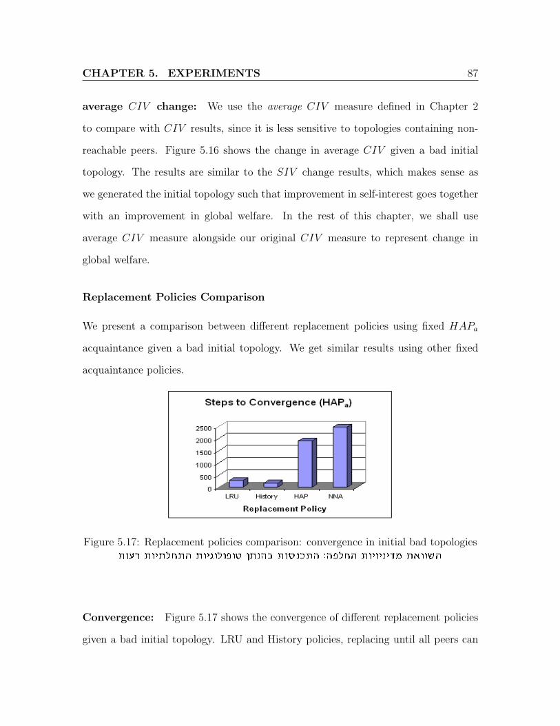
CHAPTER 5. EXPERIMENTS 87
average CIV change: We use the average CIV measure defined in Chapter 2
to compare with CIV results, since it is less sensitive to topologies containing non-
reachable peers. Figure 5.16 shows the change in average CIV given a bad initial
topology. The results are similar to the SIV change results, which makes sense as
we generated the initial topology such that improvement in self-interest goes together
with an improvement in global welfare. In the rest of this chapter, we shall use
average CIV measure alongside our original CIV measure to represent change in
global welfare.
Replacement Policies Comparison
We present a comparison between different replacement policies using fixed HAPa
acquaintance given a bad initial topology. We get similar results using other fixed
acquaintance policies.
Figure 5.17: Replacement policies comparison: convergence in initial bad topologieszerx zeizlgzd zeibeleteh ozpda zeqpkzd :dtlgd zeieipicn z`eeyd
Convergence: Figure 5.17 shows the convergence of different replacement policies
given a bad initial topology. LRU and History policies, replacing until all peers can

CHAPTER 5. EXPERIMENTS 88
translate queries with positive accuracy converge fastest at around 275 and 172 steps
respectively. HAP converges second at about 1900 steps and NNA after it at about
2470 steps. HAP80% replacing according to weakend SIV does not realy converge.
This policy is exposed to repetative replacements of peers with close SIV , resulting
in a large number of steps without convergence. Random, replacing coincidently, does
not converge as well. Both policies are not presented in the chart.
Figure 5.18: Replacement policies comparison: topology changes in initial badtopologies
zerx zeizlgzd zeibeleteh ozpda dieleteh iiepiy :dtlgd zeieipicn z`eeyd
Topology changes: Figure 5.18 shows the topology changes each policy makes
given a bad initial topology. Presented on the left chart, Random policy, making
coincidental replacements, performs changes in about 20% of the queries. HAP80%,
exposed to repetative replacements, performs changes in about 18% of the queries.
LRU and History perform the least number of changes (about 0.05% of the queries
only). The right chart presents the same data excluding Random and HAP80%
policies and we see HAP makes changes in about 1.8% of the queries and NNA a bit
more with about 2.4% of the queries.

CHAPTER 5. EXPERIMENTS 89
Figure 5.19: Replacement policies comparison: SIV change in initial bad topologieszerx zeizlgzd zeibeleteh ozpda SIV ikxra iepiy :dtlgd zeieipicn z`eeyd
SIV change: Figure 5.19 shows SIV change for each policy given a bad initial
topology. HAP policy being self-interest oriented makes the largest improvement
(about 425%). HAP80% and NNA follow with 384% and 344% respectively. Even
Random is able to improve SIV by almost 100%. LRU and History on the other
hand, do not improve SIV much (9% and 4% respectively). The fact that both
policies do not consider mapping accuracy makes them inefficient in cases such as
this where queries are translated with low accuracy. In this case, LRU and History
policies will cease making changes when every neighbor can answer all the queries
of the peer connected to it, even if the translation is very inaccurate and possibly
erronous.
CIV change: Figure 5.20 shows CIV change for each policy given a bad initial
topology. The chart shows that all the policies, although improving SIV , spoil CIV .
LRU and History policies spoil CIV by only 16% and 8% respectively and all the
other policies spoil CIV by 58%. The reason for these resutls is that all the final
CIV values achieved by Random, HAP, HAP80% and NNA policies equal to 0, while

CHAPTER 5. EXPERIMENTS 90
Figure 5.20: Replacement policies comparison: CIV change in initial bad topologieszerx zeizlgzd zeibeleteh ozpda CIV ikxra iepiy :dtlgd zeieipicn z`eeyd
for LRU and History policies only some are equal to 0. LRU and History policies,
performing a small number of replacements, do not spoil reachability in some of the
cases, while all the other policies spoil the reachability and hence achieve lower CIV .
Figure 5.21: Replacement policies comparison: average CIV measure changezerx zeizlgzd zeibeleteh ozpda average SIV ikxra iepiy :dtlgd zeieipicn z`eeyd
Average CIV change: Figure 5.21 shows the change in average CIV given a good
(left chart) and a bad initial topology (right chart). Given a good initial topology, we
see that Random policy, making many coincidental replacements spoils average CIV

CHAPTER 5. EXPERIMENTS 91
by about 75% and NNA making few replacements spoils average CIV by around
3%. Other policies make no changes to the topology and therefore do not change
average CIV . Given a bad initial topology, all the policies are able to improve aver-
age CIV . However, LRU and History policies, insensitive to translation accuracies,
achieve a minor improvement (12% and 7% respectively), while even Random pol-
icy achieves 87% improvement. HAP, HAP80% and NNA policies outperform the
other policies and achieve large improvment. HAP, being the most self-interest ori-
ented achieves 331% improvment. HAP80%, compromising on self-interest achieves
357% improvment and NNA, considering both accuracy and connectivity achieves the
largest imrovement (414%).
Figure 5.22: Replacement policies comparison: reachability change in initial badtopologies
zerx zeizlgzd zeibeleteh ozpda zeyibp iiepiy :dtlgd zeieipicn z`eeyd
Reachability change: Figure 5.22 shows reachability change for each policy given
a bad initial topology. Random decreases reachability the most with an average
change of 48% of the peers becoming non-reachable. NNA, HAP80% and HAP de-
crease reachability by making about 36%, 28% and 22% of the peers non-reachable

CHAPTER 5. EXPERIMENTS 92
respectively. LRU and History policies, making a small number of replacemnts, spoil
avewrage reachability by making about 1.2% and 0.7% of the peers non-reachable,
meaning that in many cases, reachabiliy is not spoiled. These results strengthen our
conclusion about the results for CIV change.
5.5.3 Randomly Generated Topologies
This section compares the influence of applying different replacement polices on ran-
domly generated topologies. We generate random semantic topologies using the
methodology described in Section 5.2. We calculated the average measurements
for our bad initial topologies and the results are given as follows: SIV measure
value is 0.620427669. CIV measure value is 0.014513132, reflecting preservations of
worst query translation paths, and average CIV measure value is 0.254284597, higher
then CIV since it averages rather than minimizes preservation over query translation
paths.
Acquaintance Policies Comparison
We present a comparison between different acquaintance policies using fixed replace-
ment policies given a randomly generated topology. We present results only for some
of the fixed replacement policies in cases where the results are similar using other
fixed policies.
Convergence: Figure 5.23 shows the number of steps until convergence. Ran-
dom replacement making continuous replacements does not converge in general and
therefore there is no difference between acquaintance policies. For other replacement

CHAPTER 5. EXPERIMENTS 93
Figure 5.23: Acquaintance policies comparison: convergence in randomly generatedtopologies
zi`xw` zelxben zeibeleteh ozpda zeqpkzd :zexkd zeieipicn z`eeyd

CHAPTER 5. EXPERIMENTS 94
policies, we see differences in convergence between acquaintance policies but were un-
able to establish dominance. We observe that History has low convergence variance
while HAP and NNA has higher variance.
Figure 5.24: Acquaintance policies comparison: topology changes in randomlygenerated topologies
zi`xw` zelxben zeibeleteh ozpda dibeleteh iiepiy :zexkd zeieipicn z`eeyd
Topology changes: Figure 5.24 shows the number of topology changes with each
policy. The number of topology changes performed by Random replacement pol-
icy has no relation to the selected acquaintance policy. However, we are unable to
identify a major impact of using a certain acquaintance policy with any of the other
replacement policies. We see however, that the number of replacements performed

CHAPTER 5. EXPERIMENTS 95
by each replacement policy is quite stable for each replacement policy. Therefore, we
conclude that acquaintance policies have lower impact than replacement policies on
the number of topology changes.
Figure 5.25: Acquaintance policies comparison: SIV change in randomly generatedtopologies
zi`xw` zelxben zeibeleteh ozpda SIV ikxra iepiy :zexkd zeieipicn z`eeyd
SIV change: Figure 5.25 shows SIV change for each policy given an initial random
topology. We see that replacement policies are indifferent to acquaintance policies in
the context of SIV change. We also see that HAPr replacement improves SIV more
than Historyr replacement.
CIV change: Figure 5.26 shows CIV change for each policy given an initial random
topology. We see that replacement policies are indifferent to acquaintance policies in
the context of CIV change as well. We also see that HAPr replacement spoils CIV
more than Historyr replacement. These results are also affected by CIV measure
sensitivity to peers reachability.

CHAPTER 5. EXPERIMENTS 96
Figure 5.26: Acquaintance policies comparison: CIV change in randomly generatedtopologies
zi`xw` zelxben zeibeleteh ozpda CIV ikxra iepiy :zexkd zeieipicn z`eeyd
Figure 5.27: Acquaintance policies comparison: average CIV change in randomlygenerated topologies
zelxben zeibeleteh ozpda average CIV ikxra iepiy :zexkd zeieipicn z`eeyd
zi`xw`

CHAPTER 5. EXPERIMENTS 97
Average CIV change: Figure 5.26 shows average CIV change for each policy
given an initial random topology. We notice minor differences between different aver-
age CIV change achieved by replacement topologies. Historyr replacement, making
smaller number of replacements, spoils reachability less than HAPr replacement and
hence it does not spoil CIV while HAPr does.
Figure 5.28: Acquaintance policies comparison: reachability change in randomlygenerated topologies
zi`xw` zelxben zeibeleteh ozpda zeyibp iiepiy :zexkd zeieipicn z`eeyd
Reachability change: Figure 5.28 shows reachability changes for each acquain-
tance policy given an initial random topology. We see that reachability is dependent
in the replacement policy and the selection of different acquaintance policies has no
effect on it. We also see that HAPr replacement changes topology structure such
that number of peers reachable by 2-6 peers decrease while number of non-reachable

CHAPTER 5. EXPERIMENTS 98
peers and number of highly mapped peers increase.
Replacement Policies Comparison
We present a comparison between different replacement policies using fixed acquain-
tance policies given a randomly generated topology. We present results only for some
of the fixed acquaintance policies in cases where the results are similar using other
fixed policies.
Figure 5.29: Replacement policies comparison: convergence in randomly generatedtopologies
zi`xw` zelxben zeibeleteh ozpda zeqpkzd :dtlgd zeieipicn z`eeyd

CHAPTER 5. EXPERIMENTS 99
Convergence: Figure 5.29 shows the number of steps until convergence of the dif-
ferent policies. We see that Random, and HAP80% policies perform worse and do
not converge. This is only expected as both these policies perform repetative replace-
ments, reconnecting with previously replaced neighbors. History converges fastest at
approximtely 1000 steps, and NNA converges faster than LRU, both between 1500
and 2500 steps. HAP convergence varies between 1300-3000 steps, exhibiting an
inconsistent performance compared to LRU and NNA.
Figure 5.30: Replacement policies comparison: number of topology changes inrandomly generated topologies
zi`xw` zelxben zeibeleteh ozpda dibeleteh iiepiy :dtlgd zeieipicn z`eeyd

CHAPTER 5. EXPERIMENTS 100
Topology changes: Figure 5.30 shows the number of topology changes each policy
performed. HAP80%, appearing in the top two graphs, performs the highest number
of changes (about 36% of the queries), 3 times and more than the second highest
(Random, with about 12% of the queries) and about 60 times more than the lowest
(History, with about 0.6% of the queries only). Averaging the number of changes
over the number of peers we note that HAP80% preforms around 70 changes per peer
and Random performs around 20 changes per peer, higher and close to the number of
potential neighbors per peer (24), implying repetative peer replacements. LRU and
History perform the lowest number of changes. Recall that both these policies do not
relate to the translation accuracy but rather relate to the option to translate a query
through mapping link, and will both stop performing changes as soon as each peer’s
neighbors are able to translate all the peer’s queries regardless of the translation
accuracy. HAP and NNA policies perform around 2 and 3 times more changes than
the former two, but still keep a rather small amount (about 2-3% of the number of
queries).
Figure 5.31: Replacement policies comparison: SIV change in random topologieszi`xw` zelxben zeibeleteh ozpda SIV ikxra iepiy :dtlgd zeieipicn z`eeyd

CHAPTER 5. EXPERIMENTS 101
SIV change: Figure 5.31 shows the change in SIV measure achieved by each re-
placement policy. As expected, HAP replacement which is self-interest based oriented
policy, performs best and improves SIV by almost 35% which are around 2 times
better than LRU and History policies. HAP80% which is more flexible on highest
accuracy improvement threshold, performs slightly worse than HAP and NNA policy
performs better than LRU and History but not as good as HAP oriented policies.
Note that Random policy almost does not improve SIV and in fact achieved nega-
tive improvement in some of our experiments. LRU and History policies, replacing
neihgbors that are not capable of answering queries with ones that do, achieve some
positive improvement as expected, both policies however, are sensitive to a scenario
where some peers can translate all queries but with very low accuracy in which case
they will not be replaced.
Figure 5.32: Replacement policies comparison: CIV change in random topologieszi`xw` zelxben zeibeleteh ozpda CIV ikxra iepiy :dtlgd zeieipicn z`eeyd
CIV change: Figure 5.32 shows the change in CIV measure achieved by each
replacement policy. We notice that all the policies spoil CIV by almost the same
percentage. This occurs since all the final CIV values are 0 due to the existence of

CHAPTER 5. EXPERIMENTS 102
non-reachable peers in the topology. The reason that the change is not 100% negative
is that some toopologies are associated with 0 CIV value to begin with, i.e. some
initial topologies contain non-reachable peers.
Figure 5.33: Replacement policies comparison: average CIV change in randomtopologies
zelxben zeibeleteh ozpda average CIV ikxra iepiy :dtlgd zeieipicn z`eeyd
zi`xw`
Average CIV change: Figure 5.33 shows the change in CIV measure using av-
erage over paths achieved by each replacement policy. Random performs worse and
decreases CIV by 65%. HAP, being self-interest based oriented, spoils CIV by 20%
and HAP80% by 35%. NNA, relating also to the peer connectivity in the form of
neighbors count and not only to their mapping accuracy, is more cooperative oriented
and spoils CIV by only 10%. LRU and History policies perform best as they range
between low deterioration and low improvement of CIV measure.
Reachability change: Figure 5.34 shows reachability changes for each replacement
policy given an initial random topology. We see a phenomena of decrease in medium
reachability range and increase in non-reachable and highly reachable ranges. This

CHAPTER 5. EXPERIMENTS 103
Figure 5.34: Replacement policies comparison: reachability change in randomtopologies
zi`xw` zelxben zeibeleteh ozpda zeyibp :dtlgd zeieipicn z`eeyd

CHAPTER 5. EXPERIMENTS 104
leads to a topology with a small group of highly connected peers and some other peers
that are non-reachable, such that global welfare is deteriorated. This is most obvious
in Random replacement, and then NNA and HAP80%. HAP causes less changes and
LRU and History make the leaset change in the topology. We used JUNG2 framework
Figure 5.35: Replacement policies comparison: topology change visualizationdibeleteh iiepiy ly zizefg dbvd :dtlgd zeieipicn z`eeyd
to visualize topology changes under each policy. Figure 5.35 shows a graphic visu-
alization of an initial network topology and corresponding final topologies received
2http://jung.sourceforge.net/

CHAPTER 5. EXPERIMENTS 105
from applying different replacement policies. Circles in the graph represent peers and
directed edges represent mapping links between peers. In the initial topology (top
left), 2 peers are non-reachable by the other peers. All the other peers in the inner
circle are well connected, i.e. each one is a selected neighbor of more than a single
peer. Examining the final History topology (top right), we see that the number of
non-reachable peers (in the outermost circle, close to the figure edges) increased to
5, meaning that 12% of the peers became non-reachable. Additionally, 3 more peers
(another 12% of the peers) moved from being well connected to a state of reachabil-
ity hazard, i.e., only single peer is mapped to them. Next, the final HAP topology
(bottom left) contains 8 non-reachable peers (change of 24%), and 3 peers in dan-
ger of non-reachability (chagne of 12%). Last, the final Random topology (bottom
right) contains 15 non-reachable peers (chagne of 52%), and 2 peers in danger of non-
reachability (chagne of 8%). We conclude that topology self organization algorithms,
selfishly applied by inividual peers, cannot manage topology structure and maintain
peers reachability and therefore damage the network global welfare.
5.6 Discussion
Based on our results in Section 5.5 we summarize the following conclusions:
Acquaintance Policies
We were unable to clearly identify the influence of applying different acquaintance
policies on the network. We relate these results to the following possible reasons:
• We run our experiments on a small-scale network (25 peers), leading to small
sets of available candidate non-neighbors discovered during query processes. In

CHAPTER 5. EXPERIMENTS 106
Figure 5.36: SIV Vs. Average CIV in randomly generated topologieszi`xw` zelxben zeibeleteh ozpda average CIV lenl SIV

CHAPTER 5. EXPERIMENTS 107
the absence of a large variety of candidates, acquaintance algorithms do not
have much impact.
• Our matching configuration generation methodology assigns peers with similar
schemata and queries and the acquaintance algorithms were unable to distin-
guish between peers.
Replacement Policies
• We conclude that applying a “rational” replacement policy is effective for se-
mantic topology self adjustment as all the policies performed better than the
Random policy.
• Our replacement policies were capable of identifying good self-interest oriented
topologies and made small or no changes in the presence of such topologies.
• Our replacement polices were also capable of identifying bad self-interest ori-
ented topologies and their usage lead to improvement in peers’ self-interest state,
while policies adopted from file sharing P2P systems were insensitive to trans-
lation accuracies and sometimes failed to identify and improve such topologies.
• In average, our replacement policies provide higher improvements to the self-
interest value of peers in the topology than other policies. In randomly gener-
ated topologies, our HAPr replacement policy improved SIV by 35% vs. 18%
only achieved by LRUr replacement. In the extreme case of an initial bad
topology, HAPr improved SIV by 425%, whereas LRUr improved it by 9%
only.
• Our results indicate that there is a trade-off between peers self-interest and the

CHAPTER 5. EXPERIMENTS 108
global welfare of the network. Policies improving self-interest also deteriorate
global welfare. Figure 5.36 demonstrates this; we note that for the policies
across the front, average CIV decreases with SIV increase.
• We investigated deterioration of global welfare and found an interesting phe-
nomenon that involves peers reachability. We discovered that topologies deteri-
orate to a state where a small group of peers remain connected and many peers
become non-reachable and cannot answer or propagate queries (though they
can still issue queries), thus global welfare is damaged. Topology deterioration
increases with the growing in the number of replacements, as the number of
reachable peers available for replacement constantly decreases.
• We conclude that improving global welfare by means of selfish replacement
policies is non-realistic and application of cooperative algorithms is required.
We leave this topic for future research.

Chapter 6
Discussion
6.1 Conclusions
We considered a problem of identifying semantic topologies that reduce the uncer-
tainty of query reformulations in a PDMS. First, we presented a formal model for
PDMS, extending the existing models with the concept of mapping accuracy preser-
vation reflecting the impact of schema mappings uncertainty on the quality of a query
reformulation process. We demonstrated the influence of a choice of a semantic topol-
ogy over the quality of queries in the network. Additionally, we proposed measures
(SIV , CIV , and average CIV ) for evaluation of semantic topologies, representing
different perspectives of peers local interest and network global welfare.
Next we considered the problem of finding optimal semantic topologies in an
offline setting. We presented an efficient algorithm for finding optimal topologies
maximizing SIV measure. For the problem of finding optimal topologies maximizing
CIV measure, we provided a proof that it is NP-Complete even for its most simple
case of SPSQ (Single-Peer-Single-Query).
109

CHAPTER 6. DISCUSSION 110
Then, we studied the problem of finding optimal semantic topologies in an on-
line setting. We proposed a framework for topology self organization by means of
self-interested peers individually applying algorithms for semantic links adjustment.
In detail, we introduced the semantic acquaintance and replacement problems and
demonstrated their impact on the topology self organization process. We also pre-
sented several acquaintance (HAPa, HPLa, and NNAa) and replacement (HAPr,
HAP80%r, and NNAr) policies suitable for the context of our model, analysed and
demonstrated their different characteristics.
Finally, we presented a simulation architecture we constructed according to our
PDMS model, including a framework for topology self organization using semantic
acquaintance and replacement. We implemented our policies as well as other policies
taken from the field of file sharing P2P systems, and presented an empirical analysis
of the effectiveness of their application. Our results indicated that policies consider-
ing the uncertainty of mappings, perform better in achieving optimal topologies that
maximize SIV measure. We also showed a tradeoff between SIV and CIV measures
representing a tradeoff between peers selfish interest and the network global welfare.
We demonstrated by graphic visualization the impact of non-collaborative replace-
ment algorithms on peers reachability deterioration and concluded that cooperative
algorithms are required for self organization of topologies maximizing CIV measure.
6.2 Future Work
In future work of this research, we consider the following directions:
• Re-examination of the influence of acquaintance algorithms in a larger scale
network settings.

CHAPTER 6. DISCUSSION 111
• Search of new selfish replacement algorithms that will increase self interest while
maintaining global welfare.
• Composition of cooperative protocols for topology global welfare improvement.
• Suggestion of an approximate optimal solution for cooperative-interest semantic
topologies and comparison with online solutions.
• Proving that the problem of finding optimal cooperative-interest semantic topolo-
gies that maximize the average CIV measure is also a hard one.

References
[1] Clip2. The Gnutella Protocol Specification v0.4 (Document Revision 1.2),
www9.limewire.com/developer//gnutella protocol 0.4.pdf, June 2001.
[2] K. Aberer. P-grid: a self-organizing access structure for p2p information
systems. In International Conference on Cooperative Information Systems
(CoopIS), 2001.
[3] K. Aberer, P. Cudr’e-Mauroux, A. Datta, Z. Despotovic, M. Hauswirth,
M. Punceva, and R. Schmidt. P-grid: A self-organizing structured p2p
system. ACM SIGMOD Record, 32(3), 2003.
[4] K. Aberer, P. Cudre-Mauroux, and M. Hauswirth. Start making sense:
The chatty web approach for global semantic agreements. Journal of Web
Semantics, 1(1), 2003.
[5] Karl Aberer, Philippe Cudre-Mauroux, and Manfred Hauswirth. A frame-
work for semantic gossiping. SIGMOD Record, 31(4), 2002.
[6] Karl Aberer, Philippe Cudre-Mauroux, and Manfred Hauswirth. The
chatty web: Emergent semantics through gossiping. Proceedings of the
12th International World Wide Web Conference, 2003.
112

REFERENCES 113
[7] M. Arenas, V. Kantere, A. Kementsietsidis, I. Kiringa, R. Miller, and
J. Mylopoulos. The hyperion project: From data integration to data coor-
dination, 2003.
[8] C. Batini, M. Lenzerini, and S. Navathe. A comparative analysis of
methodologies for database schema integration. ACM Computing Surveys,
18(4):323–364, December 1986.
[9] J. Berlin and A. Motro. Autoplex: Automated discovery of content for
virtual databases. In C. Batini, F. Giunchiglia, P. Giorgini, and M. Mecella,
editors, Cooperative Information Systems, 9th International Conference,
CoopIS 2001, Trento, Italy, September 5-7, 2001, Proceedings, volume 2172
of Lecture Notes in Computer Science, pages 108–122. Springer, 2001.
[10] T. Berners-Lee, J. Hendler, and O. Lassila. The semantic Web. Scientific
American, May 2001.
[11] P. Bernstein, F. Giunchiglia, A. Kementsietsidis, J. Mylopoulos, L. Serafini,
and I. Zaihrayeu. Data management for peer-to-peer computing: A vision,
2002.
[12] P.A. Bernstein and S. Melnik. Meta data management. In Proceedings of
the IEEE CS International Conference on Data Engineering. IEEE Com-
puter Society, 2004.
[13] M. Cai and M. Frank. Rdfpeers: A scalable distributed rdf repository based
on a structured peer-to-peer network. In International World Wide Web
Conference (WWW), 2004.

REFERENCES 114
[14] B. Convent. Unsolvable problems related to the view integration ap-
proach. In Proceedings of the International Conference on Database Theory
(ICDT), Rome, Italy, September 1986. In Computer Science, Vol. 243, G.
Goos and J. Hartmanis, Eds. Springer-Verlag, New York, pp. 141-156.
[15] T. H. Corman, C. E. Leiserson, and R. L. Rivest. Introduction to Algo-
rithms. MIT Press, McGraw-Hill, New York, NY, 1990.
[16] A. Crespo and H. Garcia-Molina. Routing indices for peer-to-peer systems,
2002.
[17] Philippe Cudre-Mauroux. Emergent semantics : rethinking interoperability
for large scale decentralized information systems. PhD thesis, EPFL, 2006.
[18] Watts. D and Strogatz. S. Collective dynamics of small worldnetworks.
Nature 393, 1998.
[19] H.H. Do and E. Rahm. COMA - a system for flexible combination of schema
matching approaches. In Proceedings of the International conference on
very Large Data Bases (VLDB), pages 610–621, 2002.
[20] A. Doan, P. Domingos, and A.Y. Halevy. Reconciling schemas of disparate
data sources: A machine-learning approach. In Walid G. Aref, editor, Pro-
ceedings of the ACM-SIGMOD conference on Management of Data (SIG-
MOD), Santa Barbara, California, May 2001. ACM Press.
[21] A. Doan, J. Madhavan, P. Domingos, and A. Halevy. Learning to map
between ontologies on the semantic web. In Proceedings of the eleventh
international conference on World Wide Web, pages 662–673. ACM Press,
2002.

REFERENCES 115
[22] C. Domshlak, A. Gal, and H. Roitman. Rank aggregation for automatic
schema matching. IEEE Transactions on Knowledge and Data Engineering
(TKDE), 2007. forthcming.
[23] Klement EP, Mesiar R, and Pap E. Triangular norms. Kluwer, Dordrecht,
2000.
[24] J. Euzenat et al. State of the art on current alignment techniques. Knowl-
edgeWeb Deliverable 2.2.3, http://knowledgeweb.semanticweb.org, 2004.
[25] Michalis Faloutsos, Petros Faloutsos, and Christos Faloutsos. On power-
law relationships of the internet topology. In SIGCOMM, pages 251–262,
1999.
[26] M.J. Franklin, A.Y. Halevy, and D. Maier. From databases to dataspaces: a
new abstraction for information management. SIGMOD Record, 34(4):27–
33, 2005.
[27] Modica G, Gal A, and Jamil H. The use of machine generated ontologies
in dynamic information seeking. In: Proceedings of the 9th international
conference on cooperative information systems (CoopIS 2001), September
2001.
[28] A. Gal. Managing uncertainty in schema matching with top-k schema
mappings. Journal of Data Semantics, 2006.
[29] A. Gal, G. Modica, H.M. Jamil, and A. Eyal. Automatic ontology matching
using application semantics. AI Magazine, 26(1), 2005.

REFERENCES 116
[30] Avigdor Gal, Ateret Anaby-Tavor, Alberto Trombetta, and Danilo Mon-
tesi. A framework for modeling and evaluating automatic semantic recon-
ciliation. The VLDB Journal - The International Journal on Very Large
Data Bases archive Volume 14 , Issue 1, March 2005.
[31] Steven Gribble, Alon Halevy, Zachary Ives, Maya Rodrig, and Dan Suciu.
What can databases do for peer-to-peer? WebDB Workshop on Databases
and the Web, June 2001.
[32] A. Halevy, Z. Ives, P. Mork, and I. Tatarinov. Piazza: Data management
infrastructure for semantic web applications, 2003.
[33] A. Halevy, Z. Ives, D. Suciu, and I. Tatarinov. Schema mediation in peer
data management systems. In Proc. of ICDE, 2003.
[34] B. He and K.C.-C. Chang. Making holistic schema matching robust: an
ensemble approach. In Proceedings of the Eleventh ACM SIGKDD Inter-
national Conference on Knowledge Discovery and Data Mining, Chicago,
Illinois, USA, August 21-24, 2005, pages 429–438, 2005.
[35] M.R. Horton and R. Adams. Standard for interchange of usenet messages.
Network Information Center RFC 1036, December 1987.
[36] R. Huebsch, B. Chun, J. M. Hellerstein, B. T. Loo, P. Maniatis, T. Roscoe,
S. Shenker, I. Stoica, and A. R. Yumerefendi. The architecture of pier:
an internet-scale query processor. In In Conference on Innovative Data
Systems Research (CIDR), 2005.
[37] R. Hull. Managing semantic heterogeneity in databases: A theoretical
perspective. In pods, pages 51–61. ACM Press, 1997.

REFERENCES 117
[38] Madhavan J, Bernstein PA, and Rahm E. Generic schema matching with
cupid. In: Proceedings of the international conference on very large data
bases (VLDB), September 2001.
[39] A. Kementsietsidis and M. Arenas. Data sharing through query translation
in autonomous sources, 2004.
[40] A. Kementsietsidis, M. Arenas, and R. Miller. Mapping data in peer-topeer
systems: Semantics and algorithmic issues, 2003.
[41] K.Mehlhorn and S.Naher. LEDA, A platform for combinatorial and geo-
metric computing. Cambridge University Press, 1999.
[42] M. Lenzerini. Data integration: A theoretical perspective. In Proceed-
ings of the ACM SIGACT-SIGMOD-SIGART Symposium on Principles of
Database Systems (PODS), pages 233–246, 2002.
[43] DeMichiel LG. Resolving database incompatibility: an approach to per-
forming relational operations over mismatched domains. IEEE Trans
Knowl Data Eng 1(4), 1989.
[44] DeMichiel LG. Performing operations over mismatched domains. In: Pro-
ceedings of the IEEE CS international conference on data engineering,
February 1989.
[45] J. Madhavan, P.A. Bernstein, and E. Rahm. Generic schema matching
with Cupid. In Proceedings of the International conference on very Large
Data Bases (VLDB), pages 49–58, Rome, Italy, September 2001.

REFERENCES 118
[46] J. Madhavan and A. Halevy. Composing mappings among data sources,
2003.
[47] S. Melnik, E. Rahm, and P.A. Bernstein. Rondo: A programming platform
for generic model management. In Proceedings of the ACM-SIGMOD con-
ference on Management of Data (SIGMOD), pages 193–204, San Diego,
California, 2003. ACM Press.
[48] R.J. Miller, M.A. Hernandez, L.M. Haas, L.-L. Yan, C.T.H. Ho, R. Fagin,
and L. Popa. The Clio project: Managing heterogeneity. SIGMOD Record,
30(1):78–83, 2001.
[49] Thomas Moscibroda, Stefan Schmid, and Roger Wattenhofer. On the
topologies formed by selfish peers, 2006.
[50] W. Nejdl, B. Wolf, S. Decker C. Qu, M. Sintek, A. Naeve, M. Nilsson,
M. Palm’er, and T. Risch. Edutella: a p2p networking infrastructure based
on rdf. In International World Wide Web Conference (WWW), 2002.
[51] W. Nejdl, M. Wolpers, W. Siberski, C. Schmitz, M.T. Schlosser, I. Brunk-
horst, and A. Loeser. Super-peer-based routing and clustering strategies
for rdf-based peer-to-peer networks. In International World Wide Web
Conference (WWW), 2003.
[52] W.S. Ng, B.C. Ooi, and K.L. Tan. Bestpeer: A selfconfigurable peer-to-
peer system. In International Conference on Data Engineering (ICDE),
2002.

REFERENCES 119
[53] Jurcik P. and Hanzalek Z. Construction of the bounded application-layer
multicast tree in the overlay network model by the integer linear program-
ming. 2005, Emerging Technologies and Factory Automation, 2005. ETFA
2005. 10th IEEE Conference.
[54] Christopher R. Palmer and J. Gregory Steffan. Generating network topolo-
gies that obey power laws. In Proceedings of GLOBECOM 2000, 2000.
[55] E. Rahm and P.A. Bernstein. A survey of approaches to automatic schema
matching. VLDB Journal, 10(4):334–350, 2001.
[56] S. Ratnasamy, P. Francis, M. Handley, R. Karp, and S. Shenker. A scalable
content-addressable network. In ACM SIGCOMM, 2001.
[57] C.J. Van Rijsbergen. Information retrieval. Butterworths, 1979.
[58] L. Serafini, F. Giunchiglia, J. Mylopoulos, and P. Bernstein. The local
relational model: Model and proof theory, 2001.
[59] A. Sheth and J. Larson. Federated database systems for managing dis-
tributed, heterogeneous, and autonomous databases. ACM Computing
Surveys, 22(3):183–236, 1990.
[60] Y. Shu, B.C. Ooi, and K.-L. Tan. Relational data sharing in peer-based
data management systems. SIGMOD Record, 32(3), 2003.
[61] P. Shvaiko and J. Euzenat. A survey of schema-based matching approaches.
Journal of Data Semantics, 4:146 – 171, December 2005.
[62] K. Sripanidkulchai, B. Maggs, and H. Zhang. Efficient content location
using interest-based locality in peer-to-peer systems. INFOCOM, 2003.

REFERENCES 120
[63] B. Srivastava and J. Koehler. Web service composition - Current solutions
and open problems. In Workshop on Planning for Web Services (ICAPS-
03), Trento, Italy, 2003.
[64] I. Stoica, R. Morris, D. Karger, M.F. Kaashoek, and H. Balakrishnan.
Chord: A scalable peer-to-peer lookup service for internet applications. In
ACM SIGCOMM, 2001.
[65] I. Tatarinov and A. Halevy. Efficient query reformulation in peer-data
management systems. In SIGMOD, 2004., 2004.
[66] I. Tatarinov, Z. Ives, J. amd, A. Halevy, D. Suciu, N. Dalvi, X. Dong,
Y. Kadiyaska, G. Miklau, and P. Mork. The piazza peer data management
project, 2003.
[67] Da vis LS and Roussopoulos N. Approximate pattern matching in a pattern
database system. Inf Sys 5(2), 1980.
[68] S. Voulgaris, A. Kermarrec, L. Massoulie, and M. van Steen. Exploiting
semantic proximity in peer-to-peer content searching. In 10th International
Workshop on Future Trends in Distributed Computing Systems (FTDCS
2004), November 2004.
[69] Aref WG, Barbar´a D, Johnson S, and Mehrotra S. Efficient processing
of proximity queries for large databases. In: Yu PS, Chen ALP (eds)
Proceedings of the IEEE CS international conference on data engineering,
March 1995.

zeihpnq zeibeleteh ly invr oebx`
zezyx zeqqean mipezp icqn zekxrna
zinrl zinr
lii` inr

zeihpnq zeibeleteh ly invr oebx`
zezyx zeqqean mipezp icqn zekxrna
zinrl zinr
xwgn lr xeaig
x`ez zlawl zeyixcd ly iwlg ielin myl
mircnl xhqibn
rcin ledip zqcpda
lii` inr
l`xyil ibelepkh oekn — oeipkhd hpql ybed
2007 ipei dtig f"qyz fenz

lb xecbia` 'xc zkxcda dyrp xwgn lr xeaig
ledipe diyrz zqcpdl dhlewta
dcez zxkd
dxeqnd eziigpd lr lb xecbia` 'textl dwenrd izcez z` riadl ipevxa
,llka dhlewtd zeevl dpezp dpk dcez .jxcd jxe` lkl zelirend eizevre
.iaihxhqipinc`d megza reiqde mgd qgid lr ,hxta al-yi` zicedile
zevr lr zcgein dxwed dpezp ,mixg`e lapr ,xehwie ,ibg ,micenill ixagl
dcez ,lkn miaeyge mipexg` .dkinze divaihen zepn lre miliren mipeice
ziteqpi`d mzkinze mzad` ,miaexwd iixagle izgtynl dxeqn ziwpr
.ef dcear znlyd z` exyt`y od
QUALEG itexi`d cegi`d ly ziyiyd zipkzd hwiextl dcen ip`
izenlzyda daicpd zitqkd dkinzd lr oeipkhle

mipipr okez
xi zilbp`a xivwz
1 milnq zniyx
3 `ean 1
5 . . . . . . . . . . . . . . . . . . . . . . . . . . . . . . . . . . minec mixwgn 1.1
5 . . . . . . . . . . . . . . . . . . . . . . . . . . . . . zihpnq dn`zd 1.1.1
7 . . . . . . . . zinrl zinr zezyx zeqqean mipezp icqn zekxrn 1.1.2
11 . . . . . . . . . . . . . . . . . . . . . . . . . . . . . . . . . . . xeaigd oebx` 1.2
12 . . . . . . . . . . . . . . . . . . . . . . . . . . . . . . . . . . zixwir dnexz 1.3
14 lcend zxcbd 2
15 . . . . . . . . . . . . . . . . . . . . . . . . . . . . . . . . . . . mipezpd lcen 2.1
16 . . . . . . . . . . . . . . . . . . . . . . . . . . . . . . . . . . . . zyxd lcen 2.2
16 . . . . . . . . . . . . . . . . . . . . . . . . . . . . . miihpnq miietin 2.2.1
18 . . . . . . . . . . . . . . . . . . . . . . . . . . . . . . zezli`y zvtd 2.2.2
20 . . . . . . . . . . . . . . . . . . . . . . . . . . . . zihpnq dibeleteh 2.2.3
21 . . . . . . . . . . . . . . . . . . . . . . . . . . . . . . . . . . dn`zdd lcen 2.3
22 . . . . . . . . . . . . . . . . . . . . . . . . . . . . . . miietind zepekp 2.3.1
b

c mipipr okez
26 . . . . . . . . . . . . . . . . . . . . . . . . . . . ietind zepekp xeniy 2.3.2
31 . . . . . . . . . . . . . . . . . . . . . . . . zeihpnq zeibeleteh ly dkxrd 2.4
32 . . . . . . . . . . . . . . iyi` qxhpi` qiqa lr zeibeleteh zkxrd 2.4.1
34 . . . . . . . . . . . . . szeyn qxhpi` qiqa lr zeibeleteh zkxrd 2.4.2
37 zeilnihte` zeihpnq zeibeleteh lr 3
38 . . . . . . . . . . . . . . . iyi` qxhpi` qiqa lr zeilnihte` zeibeleteh 3.1
40 . . . . . . . . . . . . . . szeyn qxhpi` qiqa lr zeilnihte` zeieleteh 3.2
42 . . . . zebxc iveli` mr zilnipind lelqnd zltkn meniqwn ur 3.2.1
dzli`ye cigi zinr xear zilnihte` dibeleteh z`ivn ziira 3.2.2
50 . . . . . . . . . . . . . . . . . . . . . . . . . . . . . . . . . . . . dcigi
52 . . . . . . . . . . . . . . . . . . . . . . . . . . . . . . . . . . . . . . . . . oeic 3.3
54 zi`nvr zepbx`zne zepzyn zeibeleteh 4
55 . . . . . . . . . . . . . . . . . . . . . . . . . . . . . . . . . . zihpnq zexkd 4.1
61 . . . . . . . . . . . . . . . . . . . . . . . . . . . . . . . . . . zihpnq dtlgd 4.2
67 miieqip 5
67 . . . . . . . . . . . . . . . . . . . . . . . . . . . . . . . . . divleniqd dpan 5.1
72 . . . . . . . . . . . . . . . . . . . . . . . . . . . . . . . . . . . . . . . mipezp 5.2
75 . . . . . . . . . . . . . . . . . . . . . . . . . . . . . . . . . . miieqipd dpan 5.3
76 . . . . . . . . . . . . . . . . . . . . . . . . . . . . . . . . . . . . . . . miccn 5.4
78 . . . . . . . . . . . . . . . . . . . . . . . . . . . . . . . . . . . . . . . ze`vez 5.5
78 . . . . . . . . . . . . . . . . . . . . . . zeaeh zeizlgzd zeibeleteh 5.5.1
82 . . . . . . . . . . . . . . . . . . . . . . . zerx zeizlgzd zeibeleteh 5.5.2
92 . . . . . . . . . . . . . . . . . . . . . . zi`xw` zellegn zeibeleteh 5.5.3

d mipipr okez
105 . . . . . . . . . . . . . . . . . . . . . . . . . . . . . . . . . . . . . . . . . oeic 5.6
109 oeic 6
109 . . . . . . . . . . . . . . . . . . . . . . . . . . . . . . . . . . . . . . . ze`vez 6.1
110 . . . . . . . . . . . . . . . . . . . . . . . . . . . . . . zicizr dcear jynd 6.2
111 zexewn zniyx
k xivwz

mixei` zniyx
17 . . . . . . . . . . . . . . . . . . . . . . . . . . . . . . dzli`y mebxzl dnbec 2.1
18 . . . . . . . . . . . . . . . . . zinrl zinr zyxa mipezp icqn lcen xe`iz 2.2
miietin zervn`a zexaegn mizinr ly zenkq ea ,zihpnq zyx sxb 2.3
19 . . . . . . . . . . . . . . . . . . . . . . . . . . . . . . . . . . . . . . miihpnq
lr ueli` mr dibeletehe zezli`y mebxz zeaky :zihpnqd zyxd lcen 2.4
21 . . . . . . . . . . . . . . . . . . . . . . . . . . . . . . . . . . . mipkyd xtqn
24 . . . . . . . . . . . . . . . . . . . . . . . . . . . . . . miietin zepekpl dnbec 2.5
28 . . . . . . . . . . . . . . . . . . . . . . . . . . miietin zepekp xeniyl dnbec 2.6
30 . . . . . . . . . . . . . . . . . . . . . . . dzli`y ly ly mebxz sxbl dnbec 2.7
33 . . . . . miietin zepekp lr zqqaznd zihpnq dibeleteh zkxrdl dnbec 2.8
41 . . . CIV jxr z` meniqwnl d`iand dibeleteh z`ivn ziira ly beeiq 3.1
44 zeilniqwn zeltkn urle zilnipind lelqnd zltkn meniqwn url dnbec 3.2
46 . . . . . . . . . . . . . . . . . . . SPT ziiral MPT ziiran xarnl dnbec 3.3
47 . . . . . . . . . . . . . . . . . . . . . . db-MMPT znerl MMPT-l dnbec 3.4
50 . . . . . . . . . . . . . . . db-MMPT ziiral ATSP ziiran xarnl dnbec 3.5
52 . . . . . . . . . . . . . . . SPSQ ziiral db-MMPT ziiran xarnl dnbec 3.6
56 . . . . . . . . . . . . . . . . . . . . . . . . . mixiyw izla miihpnq miaikx 4.1
e

f mixei` zniyx
60 . . . . . . . . . . . . . . . . . . . . . . . . . . . . . zexkd zeieipicnl dnbec 4.2
63 . . . . . . . . . . . . . . . . . . . . . . . . . . . . . dtlgd zeieipicnl dnbec 4.3
68 . . . . . . . . . zezli`y itqe`e zenkq ,mibyen mler :divleniqd lcen 5.1
70 . . . . . . zezli`y mebxz zeakye zihpnq dibeleteh :divleniqd lcen 5.2
71 . . . . . . . . dcigi dzli`y xear zelert svx miyxz :divleniqd lcen 5.3
73 . . . . . . . . . zyxa mixagd ly zenkqa mibyen zellkidl zexazqd 5.4
74 . . . . . . . . . . mipeye midf mibyen xear zezli`yd zepekp zeiebltzd 5.5
74 . . power law zeiweg zniiwn bexic lenl d`ivi zbxc :zyxd ziibeleteh 5.6
79 zeaeh zeizlgzd zeibeleteh ozpda zeqpkzd :dtlgd zeieipicn z`eeyd 5.7
zeizlgzd zeibeleteh ozpda dibeleteh iiepiy :dtlgd zeieipicn z`eeyd 5.8
80 . . . . . . . . . . . . . . . . . . . . . . . . . . . . . . . . . . . . . . . . zeaeh
zeizlgzd zeibeleteh ozpda SIV ikxra iepiy :dtlgd zeieipicn z`eeyd 5.9
81 . . . . . . . . . . . . . . . . . . . . . . . . . . . . . . . . . . . . . . . . zeaeh
zeizlgzd zeibeleteh ozpda CIV ikxra iepiy :dtlgd zeieipicn z`eeyd 5.10
81 . . . . . . . . . . . . . . . . . . . . . . . . . . . . . . . . . . . . . . . . zeaeh
83 . zerx zeizlgzd zeibeleteh ozpda zeqpkzd :zexkd zeieipicn z`eeyd 5.11
zeizlgzd zeibeleteh ozpda dibeleteh iiepiy :zexkd zeieipicn zee`yd 5.12
84 . . . . . . . . . . . . . . . . . . . . . . . . . . . . . . . . . . . . . . . . . zerx
zeizlgzd zeibeleteh ozpda SIV ikxra iepiy :zexkd zeieipicn z`eeyd 5.13
84 . . . . . . . . . . . . . . . . . . . . . . . . . . . . . . . . . . . . . . . . . zerx
zeizlgzd zeibeleteh ozpda CIV ikxra iepiy :zexkd zeieipicn z`eeyd 5.14
85 . . . . . . . . . . . . . . . . . . . . . . . . . . . . . . . . . . . . . . . . . zerx
86 zerx zeizlgzd zeibeleteh ozpda zeyibpa iepiy :zexkd zeieipicn z`eeyd 5.15

g mixei` zniyx
zeieleteh ozpda average CIV ikxra iepiy :zexkd zeieipicn z`eeyd 5.16
86 . . . . . . . . . . . . . . . . . . . . . . . . . . . . . . . . . . zerx zeizlgzd
87 . zerx zeizlgzd zeibeleteh ozpda zeqpkzd :dtlgd zeieipicn z`eeyd 5.17
zeizlgzd zeibeleteh ozpda dieleteh iiepiy :dtlgd zeieipicn z`eeyd 5.18
88 . . . . . . . . . . . . . . . . . . . . . . . . . . . . . . . . . . . . . . . . . zerx
zeizlgzd zeibeleteh ozpda SIV ikxra iepiy :dtlgd zeieipicn z`eeyd 5.19
89 . . . . . . . . . . . . . . . . . . . . . . . . . . . . . . . . . . . . . . . . . zerx
zeizlgzd zeibeleteh ozpda CIV ikxra iepiy :dtlgd zeieipicn z`eeyd 5.20
90 . . . . . . . . . . . . . . . . . . . . . . . . . . . . . . . . . . . . . . . . . zerx
zeibeleteh ozpda average SIV ikxra iepiy :dtlgd zeieipicn z`eeyd 5.21
90 . . . . . . . . . . . . . . . . . . . . . . . . . . . . . . . . . . zerx zeizlgzd
91 zerx zeizlgzd zeibeleteh ozpda zeyibp iiepiy :dtlgd zeieipicn z`eeyd 5.22
93 zi`xw` zelxben zeibeleteh ozpda zeqpkzd :zexkd zeieipicn z`eeyd 5.23
zelxben zeibeleteh ozpda dibeleteh iiepiy :zexkd zeieipicn z`eeyd 5.24
94 . . . . . . . . . . . . . . . . . . . . . . . . . . . . . . . . . . . . . . . zi`xw`
zelxben zeibeleteh ozpda SIV ikxra iepiy :zexkd zeieipicn z`eeyd 5.25
95 . . . . . . . . . . . . . . . . . . . . . . . . . . . . . . . . . . . . . . . zi`xw`
zelxben zeibeleteh ozpda CIV ikxra iepiy :zexkd zeieipicn z`eeyd 5.26
96 . . . . . . . . . . . . . . . . . . . . . . . . . . . . . . . . . . . . . . . zi`xw`
zeibeleteh ozpda average CIV ikxra iepiy :zexkd zeieipicn z`eeyd 5.27
96 . . . . . . . . . . . . . . . . . . . . . . . . . . . . . . . . . zi`xw` zelxben
97 zi`xw` zelxben zeibeleteh ozpda zeyibp iiepiy :zexkd zeieipicn z`eeyd 5.28
98 zi`xw` zelxben zeibeleteh ozpda zeqpkzd :dtlgd zeieipicn z`eeyd 5.29
zelxben zeibeleteh ozpda dibeleteh iiepiy :dtlgd zeieipicn z`eeyd 5.30
99 . . . . . . . . . . . . . . . . . . . . . . . . . . . . . . . . . . . . . . . zi`xw`

h mixei` zniyx
zelxben zeibeleteh ozpda SIV ikxra iepiy :dtlgd zeieipicn z`eeyd 5.31
100 . . . . . . . . . . . . . . . . . . . . . . . . . . . . . . . . . . . . . . . zi`xw`
zelxben zeibeleteh ozpda CIV ikxra iepiy :dtlgd zeieipicn z`eeyd 5.32
101 . . . . . . . . . . . . . . . . . . . . . . . . . . . . . . . . . . . . . . . zi`xw`
zeibeleteh ozpda average CIV ikxra iepiy :dtlgd zeieipicn z`eeyd 5.33
102 . . . . . . . . . . . . . . . . . . . . . . . . . . . . . . . . . zi`xw` zelxben
103 . . zi`xw` zelxben zeibeleteh ozpda zeyibp :dtlgd zeieipicn z`eeyd 5.34
104 . . . . . . . dibeleteh iiepiy ly zizefg dbvd :dtlgd zeieipicn z`eeyd 5.35
106 . . . . . . . zi`xw` zelxben zeibeleteh ozpda average CIV lenl SIV 5.36

ze`lah zniyx
61 . . . . . . . . . . . . . . . . . . . . . . . . . . zexkd zeieipicn zkxrd iccn 4.1
62 . . . . . . . . zepey zexkd zeieipicn it lr mixgap mizinrl ietin zepekp 4.2
65 . . . . . . . . . . . . . . . . . . . . . . . . . dtlgd zeieipicn zkxrd iccn 4.3
72 . . . . . . . . . . . . . . . . . . . . . . . . . . . . . . . divleniql mixhnxt 5.1
75 . . . . . . . . . . . . . . . . . . . . divleniqd zvixl mixhnxt ly mekiq 5.2
i

xivwz
zezyxa zeievnd zepekz zealyn zinrl zinr zezyx zeqqean mipezp icqn zekxrn
-iwd zepekz mr cgi ,zyxa mixagd ly dinepehe`e zxfean daiaq :oebk zinrl zinr
lk .zeakxen zezli`y ly drad zlekie ihpnq xyer :oebk mipezp icqn zekxrna zeni
x`yl mipezpd qiqa z` zx`znd dnkq bivne inewn mipezp qiqa ldpn zyxa zinr
-i` ote`a zezli`y zvtd zervn`a dyrp df beqn zyxa rcin seziy .zyxa mizinrd
xiyrd lcena yeniya mihlead zepexzidn cg` .zyxa mixyewn mizinr oia iaihxh
-na zeniiwd dzli`yd zetya ynzydl zlekia uerp mipezp icqn zekxrn ly okeza
zezli`y geqip xyt`nd drad xyer zelra ode ,(SQL, XQeury ,lynl) df beqn zekxr
.zeakxen
ick zenkq oia zihnehe` dn`zdl zewipkha miynzyn df beqn zyxa mixagd
miietin .mdly mipezpd iqiqa z` zex`znd zenkqd oia miihpnq miietin xevil
lr zeprl zlekid ,zinr lkl .zezli`y zervn`a rcin seziyl qiqak miynyn el`
miniiwd migpen xnelk ,cala ely dnkqdn migewld migpena zegqepnd zezli`y
ly dnkqn migewld migpena zgqepnd dzli`y ozpda ,ok lr .ely mipezpd qiqaa
-nyn zlra dzli`yl z`f dzli`y mbxzl eilr dney ,xewn znkq oldl ,edylk zinr
,cri znkq oldl ,xg` zinr ly dnkqn wxe j` migewld migpena zgqepnd ddf zer
beqn mebxz .zernyn zelra zeaeyz lawle df zinrl dzli`yd z` xiardl epevxa m`
.crid znkql xewnd znkq oia ihpnq ietina yeniy jez revial ozip df
k

l xivwz
rcin mix`znd mibyen oia jeciy rvazn ea jildz `ed zenkq oia zihpnq dn`zd
jildz ly xvezd ,ihnkq ietin .dpey milin xve` e`/e dpan zelra zenkqa mi`vnpd
znkqa mi`vnpd mibyenl idylk xewn znkqa mi`vnpd mibyen oia mebxz x`zn ,df
zx`eznd dzli`y xiardl ozip ,df beqn mebxz zervn`a .ddf zernyn ilra mde cri
zervn`a zgqepnde ddf zernyn zlra dzli`yl xewnd znkqn mibyena yeniy jez
lr xewna rvazd zihpnqd dn`zdd jildz ,ezeakxen lya .crid zknq jezn mibyen
yeniy aiign zinrl zinr zezyx ly lcebd xcq ,mxa .[14, 37] cala iyep` dgnen ici
dxeva rveand zihnehe` dn`zd jildz .zeihpnq zen`zd revial zepkenn zehiya
milawznd miietinde ,ze`ce i` ly zniieqn dcin eaega onehd jildzk gked ,zpkenn
.miieby zeidl s`e weic xqegn leaql miieyr ,ef dxeva jildzd zlrtdn d`vezk
lkl ea ,zihpnq dn`zda dpenhd ze`ced i` zkxrdl lcen rivd [30] mcew xwgn
.ietind mzixebl` ici lr zytzp `idy itk ezepin` z` swynd zepekp ccn jieyn ietin
zlertn lawznd mlyend ietinl aexw ,oin` ietin swyn deab zepekp ccn lra ietin
ihxe`iz gezip zervn`a xwgnd bivd ,sqepa .iyep` dgnen ici lr zrvaznd dn`zd
ozip mxear ,"miipehepen" mi`xwpe dxecq dxeva mibdpznd miietin ly dgtyn ,iieqipe
minzixebl`l qgiizdl ozip ,jkitl .oin` ietin swyn ok` deab zepekp ccny reawl
mitwynd mipin` minzixebl` l`k ,zeipehepend zpekz z` miniiwnd miietin mibivnd
.mirivn md mze` miietind ly zepekpd ccn z` wiecn ic ote`a
zeki` lr drityn zyxa mixag oia ze`ce ixqg ietin ixyw ly mze`vnid zcaer
jez zenbxeznd zezli`y .l`eyl zexfgend ze`vezd lre da zevtend zezli`yd
opi`y ze`vez xifgdle dpey zernyn lawl zeieyr miwiiecn mpi`y miietina yeniy
lk ly miietind sqe`l ok m` dax zeaiyg qgiil ozip .zixewnd dzli`yl zexeyw
.zyxa zezli`yd zvtd jildz zeki` lr dax drtyd el` miietinl oky ,zyxa xag
eze` ly ziyi`d mipkyd zxigan xiyi ote`a xfbp zyxa zinr lk ly miietind sqe`
dxiga .zyxa )dibeleteh( mixywd dpann zxfbp zyxa miietind sqe` ,dllkdae ,zinr

n xivwz
ly ze`ceed i` zcin z` mvnvl dieyr zinr lkl xyewnd mipkyd sqe` ly zlkyen
inebxza weicd xqeg znx z` oihwdl ,`vei lretke zyxa mitzzynd oia miietind
.zelawznd ze`vezd zeki` z` xtyle zezli`yd
,zinrl zinr zezyx zeqqean mipezp icqn zekxrnl miqgiizn ep` ,z`f dceara
meiw migipn ep` .mitzzynd oia ietind ixywa ze`ce i` ly zniieqn dcin zniiw oda
`ede ,zyxl zetxhvdd zra mixag xtqnl zi`xw` xagzn zinr lk da dpzyn daiaq
x`eznk daiaq ozpda .zyxa ezelirt ztewz jldna el` mixyw okcrle zepyl ieyr
:od mibivn ep`y zeixwird zel`yd ,lirl
i` znx z` zenvnvnd el`k ,"zeaeh" zeibeleteh liri ote`a `evnl ozip m`d •
?zyxa ze`ced
ici lr myeind invr oebx` zervn`a el`k "zeaeh" zeibeleteh `evnl ozip m`d •
?miiyi` miqhxpi` qiqa lre i`nvr ote`a milretd zyxa mixag
ilnxet lcen bivp oey`xd wlga .miixwir miwlg drax`l dfizd z` miwlgn ip`
-ietin ly ze`ced i`a aygznd zinrl zinr zyx lr zqqeand mipezp icqn zekxrnl
zeihpnq zeibeleteh z`ivn ly diraa oecp ipyd wlga .zyxa zezli`y lr dzrtyde mi
z` meniqwnl ze`iand zeibeletehl od qgiizp ,zyxd lr `ln rcin ozpda zeilnihte`
ly zllekd zeki`d z` meniqwnl ze`iand zeibeletehl ode zinr ly iyi`d qxhpi`d
ribdl oeiqpae zeihpnq zeibelteh ly invr oebx`a oecp ,iyilyd wlga .zyxa zezli`y
invr oebx`l zehiy bivp df wlga .zyxd lr `ln rcin xcrida zeilnihte` zeibeletehl
bivp ,oexg`d wlga .zyxa miaeh mipky ly dxigae iedifl zexeywd zeiral qgiizpe
df wxta .epbvdy lcend z` zn`ezd zinrl zinr zyxa mipezp icqn dncnd ieqip
.zeihpnq zeibeleteh ly invr oebx`l zepey zeieipicn oia d`eeyd ze`vez bivp

p xivwz
:lcend zxcbd
i` zrtyd ly zil`nxet dbvd rivne [6] miniiw milcenl dagxd deedn eply lcend
bviind ccn mirivn ep` .zyxa zezli`y zeki` lr ihpnq ietina zniiwd ze`ced
zezli`y mebxz jldna rvaznk miawer miietin aizp jxe`l ietind zepekp xeniy z`
aizpa mincwzny lkk mebxzd zepekp zkirc zrtez z` zizenk bviin df ccn .zyxa
zervn`a .zexfgend ze`vezd zeki`a mebtl dieyrd drtez ,zezli`yd ly mebxzd
-ibeleteh( dpan zkxrdl miccn mirivn ep` ,zepekpd xeniy ccne mebxzd zepekp ccn
hand zcewpn od zyxa zezli`y ly mebxzd zeki` z` mibviind zihpnq zyx )zi
.szeyn qxhpi` jezn zelkzqda ode xag lk ly ziyi`d
:`ln izyx rcin ozpda zeilnihte` zeibeleteh z`ivn
qiqa xeza ,oeewn `l ote`a zeilnihte` zeibeleteh z`ivn ly diraa mipiiprzn ep`
mzixebl` mibivn ep` .zpeewn dxeva invr oebx` jez zelawznd zeibeleteh ly dkxrdl
iyi` qxhpi`d z` bviind ccnd z` meniqwnl ze`iand el`k zeibeleteh z`ivnl liri
ze`iand zeibeleteh z`ivn ly dirady mi`xn ep` ,z`f znerl .zyxa xag lk ly
ep` .dyw dira `id zyxa mixagl szeynd qxhpi`d z` bviind ccnd z` meniqwnl
dirad ,xzeia heytd dxwnd xeary mi`xne mixwn xtqnl dirad ly beeiq mirvan
.il`inepilet onfa oexztl zpzip `l
:zeihpnq zeibeleteh ly invr oebx`
zyxd lk lr `ln rcin zyxa xag s`l oi` ,zinrl zinr zezyxa ifkxn ledip xcrida
dlabn zgz zeilnihte` zeibeleteh z`ivn ly zpeewnd diraa mifkxzn ep` jkitle
zeihqixeid zehiy zervn`a zeibeleteh ly invr oebx`l zxbqn mirivn ep` .z`f
zexkdd ziira z` mibivn ep` z`f zxbqn zgz .zihpnqd zyxa mipky zxigae iedifl
zwqerd dtlgdd ziira z`e zihpnq daxiw ilra miil`ivphet mipky iedifa zwqerd

q xivwz
zeiradn zg` lkl .zihpnq daxiw iccn it lr mixg` ipt lr minieqn mixag ztcrda
.meyiil zeixyt` zehiy xtqn migzpne mirivn ep`
: ze`vez
zn`ezd zinrl zinr zyx iab lr mipezp icqn xear epgzity dincd zaiaq mibivn ep`
mipky zxigae iedifl zeihqixeid zehiyd z` epnyii ,z`f daiaqa .eply lcend z`
megzn zele`yd zepey zehiy mb enk zeihpnq zeibeleteh ly invr oebx` xear eprvdy
oebx` zehiy zlrtd ik dler eply miieqipd on .zinrl zinr zezyxa mivawd seziy
qxhpi`d jxr ccn z` meniqwnl ze`iand zeihpnq zeibeleteh z`ivnl dliri invr
miihpnq miietina zniiwd ze`ced i`a zeaygznd zehiy ike zyxa xag lk ly iyi`d
ccn xetiy jez zyxd iepiyy ep`xd ,ok enk .z`f dxhnl zexg` zehiy lr zeticr
zeki`ae szeynd qxhpi`d ccna rebtle ybpzdl ieyr ,xag lk ly iyi`d qxhpi`d
zeihqixeid zehiy eit lr gezip mibivn ep` ,seqal .zyxa zezli`y mebxz ly zllekd
mixag ly zllekd zeyibpa zenbet zyxa mixag ici lr zi`nvr zelrtend invr oebx`l
zlrtd zyxcpy dler o`kn .zyxa zezli`y ly mebxzd zlekia mb jkitle zyxa
szeynd qxhpi`d z` meniqwnl ze`iand zeibelteh biydl zpn lr szeyn lewehext
.zyxd ly in`pic oebx` ly mirvn`a


![Organizing knowledge in Semantic Web - cvut.cz · Relationship lists (thesauri, semantic networks, ontologies) another classification [hedden2010accidental] defines Controlled vocabularies](https://static.fdocuments.net/doc/165x107/5ec910c81b72bc186b68c2da/organizing-knowledge-in-semantic-web-cvutcz-relationship-lists-thesauri-semantic.jpg)