Self-Modulated Dynamics of Relativistic Charged Particle ... · Self-Modulated Dynamics of...
174
Self-Modulated Dynamics of Relativistic Charged Particle Beams in Plasmas SUBMITTED AS PARTIAL FULFILLMENT OF THE REQUIREMENTS FOR THE DEGREE OF DOCTOR OF PHILOSOPHY IN FUNDAMENTAL AND APPLIED PHYSICS Supervisor: Professor Renato Fedele Co-supervisors: Dr. Sergio De Nicola Professor Dusan Jovanovi´ c Candidate: Tahmina Akhter XXVIII cycle DIPARTIMENTO DI FISICA “ETTORE PANCINI” UNIVERSIT ` A DEGLI STUDI DI NAPOLI FEDERICO II MARCH 31, 2016 NAPOLI, ITALY
Transcript of Self-Modulated Dynamics of Relativistic Charged Particle ... · Self-Modulated Dynamics of...

Self-Modulated Dynamics of Relativistic Charged Particle
Beams in Plasmas
SUBMITTED AS PARTIAL FULFILLMENT OF THE
REQUIREMENTS FOR THE DEGREE OF
DOCTOR OF PHILOSOPHY
IN
FUNDAMENTAL AND APPLIED PHYSICS
Supervisor:
Professor Renato Fedele
Co-supervisors:
Dr. Sergio De Nicola
Professor Dusan Jovanovic
Candidate:
Tahmina Akhter
XXVIII cycle
DIPARTIMENTO DI FISICA “ETTORE PANCINI”
UNIVERSITA DEGLI STUDI DI NAPOLI FEDERICO II
MARCH 31, 2016
NAPOLI, ITALY
UNIVERSITA DEGLI STUDI DI NAPOLI FEDERICO II
DIPARTIMENTO DI FISICA “ETTORE PANCINI”
The undersigned hereby certify that they have read and recommended to
the Fundamental and Applied Physics for acceptance a thesis entitled “Self-
Modulated Dynamics of Relativistic Charged Particle Beams in Plasmas”
by Tahmina Akhter as partial fulfillment of the requirements for the degree of
Doctor of Philosophy.
Dated: March 31, 2016
Research Supervisor:Professor Renato Fedele
Co-Supervisors:Dr. Sergio De Nicola
Professor Dusan Jovanovic
PhD Coordinator:Professor Raffaele Velotta
Examiners:
ii

UNIVERSITA DEGLI STUDI DI NAPOLI FEDERICO II
Date: March 31, 2016
Author: Tahmina Akhter
Title: Self-Modulated Dynamics of Relativistic Charged Particle
Beams in Plasmas
Department: Dipartimento di Fisica “Ettore Pancini”
Degree: PhD
Signature of Author
iii

To my husband MD. ASHADUZZAMAN
iv
Contents
List of Figures viii
List of Symbols xii
List of Acronyms xv
Acknowledgements xvi
Abstract xviii
Introduction 1
1 Models for plasmas 201.1 Preliminary considerations . . . . . . . . . . . . . . . . . . . . . . . . . . 201.2 Fluid theory of a nonrelativistic plasma:
the Lorentz-Maxwell system . . . . . . . . . . . . . . . . . . . . . . . . . 261.3 Kinetic description of a relativistic plasma . . . . . . . . . . . . . . . . . . 301.4 Fluid description of a relativistic plasma . . . . . . . . . . . . . . . . . . . 321.5 Collisional plasmas . . . . . . . . . . . . . . . . . . . . . . . . . . . . . . 331.6 Conclusions . . . . . . . . . . . . . . . . . . . . . . . . . . . . . . . . . . 35
2 The theory of plasma wake field excitation: the Poisson-type equation 362.1 Introduction . . . . . . . . . . . . . . . . . . . . . . . . . . . . . . . . . . 372.2 Definition of plasma wake field . . . . . . . . . . . . . . . . . . . . . . . . 382.3 Lorentz-Maxwell system of equations for the
beam-plasma system . . . . . . . . . . . . . . . . . . . . . . . . . . . . . 412.4 Poisson-type equation in overdense regime: collisionless nonrelativistic plasma 432.5 Ultrarelativistic driver in a cold plasma: longitudinal sharpness regimes . . 482.6 Ultrarelativistic driver in a cold plasma: transverse sharpness regimes . . . 502.7 Poisson-type equation for purely longitudinal case . . . . . . . . . . . . . . 522.8 Poisson-type equation for purely transverse case . . . . . . . . . . . . . . . 53
v
2.9 Conclusions . . . . . . . . . . . . . . . . . . . . . . . . . . . . . . . . . . 54
3 Models for charged particle beams and its self-consistent interaction with thesurrounding medium 553.1 Preliminary considerations . . . . . . . . . . . . . . . . . . . . . . . . . . 563.2 Relativistic Hamiltonian for a single-particle motion in the presence of EM
fields . . . . . . . . . . . . . . . . . . . . . . . . . . . . . . . . . . . . . . 573.2.1 Slightly perturbed motion . . . . . . . . . . . . . . . . . . . . . . 583.2.2 Perturbed effective single particle Hamiltonian . . . . . . . . . . . 58
3.3 The Vlasov equation for a relativistic charged-particle beam . . . . . . . . 613.4 The Vlasov-Poisson-type system of equations . . . . . . . . . . . . . . . . 613.5 Conclusions . . . . . . . . . . . . . . . . . . . . . . . . . . . . . . . . . . 62
4 Transverse self-modulated beam dynamics of a nonlaminar, ultra-relativisticbeam in a non relativistic cold plasma 644.1 Introduction . . . . . . . . . . . . . . . . . . . . . . . . . . . . . . . . . . 654.2 The governing equations of the transverse beam dynamics . . . . . . . . . 674.3 Beam envelope description . . . . . . . . . . . . . . . . . . . . . . . . . . 69
4.3.1 First virial equation . . . . . . . . . . . . . . . . . . . . . . . . . . 714.3.2 Second virial equation . . . . . . . . . . . . . . . . . . . . . . . . 734.3.3 Virial description and constants of motion . . . . . . . . . . . . . . 744.3.4 Constants of motion and envelope equations . . . . . . . . . . . . . 754.3.5 Beam emittance . . . . . . . . . . . . . . . . . . . . . . . . . . . . 764.3.6 Cylindrical Symmetry . . . . . . . . . . . . . . . . . . . . . . . . 79
4.4 Self-modulated beam dynamics in purely local regime . . . . . . . . . . . 794.4.1 Unmagnetized plasma . . . . . . . . . . . . . . . . . . . . . . . . 814.4.2 Magnetized plasma . . . . . . . . . . . . . . . . . . . . . . . . . . 834.4.3 Transverse beam emittance and equivalent Gaussian beam . . . . . 84
4.5 Self modulation in strongly nonlocal regime . . . . . . . . . . . . . . . . . 884.5.1 Aberration-less approximation . . . . . . . . . . . . . . . . . . . . 894.5.2 Self-modulation analysis by means of the Sagdeev potential . . . . 92
4.6 Qualitative stability analysis . . . . . . . . . . . . . . . . . . . . . . . . . 954.7 Quantitative analysis of beam self-modulation in the arbitrary regime . . . . 98
4.7.1 General solution of Uw . . . . . . . . . . . . . . . . . . . . . . . . 984.7.2 Envelope equation and Sagdeev potential in the general case . . . . 1014.7.3 Analysis of the envelope self-modulation in the general case . . . . 103
4.8 Conclusions . . . . . . . . . . . . . . . . . . . . . . . . . . . . . . . . . . 107
vi
5 Longitudinal instability analysis of beam-plasma system 1095.1 Introduction . . . . . . . . . . . . . . . . . . . . . . . . . . . . . . . . . . 1105.2 Dispersion relation . . . . . . . . . . . . . . . . . . . . . . . . . . . . . . 1125.3 Monochromatic profile . . . . . . . . . . . . . . . . . . . . . . . . . . . . 1135.4 Non-monochromatic case: weak Landau damping and instability . . . . . . 1155.5 Conclusions . . . . . . . . . . . . . . . . . . . . . . . . . . . . . . . . . . 119
6 The coupling impedance concept for PWF self-interaction 1206.1 Introduction . . . . . . . . . . . . . . . . . . . . . . . . . . . . . . . . . . 1206.2 Phenomenological platform of the beam-plasma interaction . . . . . . . . . 1236.3 Vlasov-Poisson-type pair of equations . . . . . . . . . . . . . . . . . . . . 1246.4 Heuristic definition of coupling impedance . . . . . . . . . . . . . . . . . . 1256.5 Stability analysis . . . . . . . . . . . . . . . . . . . . . . . . . . . . . . . 125
6.5.1 Monochromatic beam . . . . . . . . . . . . . . . . . . . . . . . . 1266.5.2 Non-monochromatic beam . . . . . . . . . . . . . . . . . . . . . . 127
6.6 Collisional beam-plasma system . . . . . . . . . . . . . . . . . . . . . . . 1286.7 Conclusions . . . . . . . . . . . . . . . . . . . . . . . . . . . . . . . . . . 131
Conclusions and Remarks 133
A Virial descriptions 136
B Envelope descriptions 143
List of Publications/Communications 146
Bibliography 150
vii

List of Figures
1 Scheme of the laser wakefield acceleration excited by a laser pulse. The
driving laser pulse interacts with the active medium plasma and produces a
driven system (charged particle beam) which leads to acceleration. . . . . . 5
2 Plasma wake field acceleration scheme, excited by a relativistic electron
beam, where the beam interacts with the surrounding plasma and thereby
produces an wake field behind the beam itself. . . . . . . . . . . . . . . . . 7
4.1 Beam envelope surface that, at each τ, is described by x2 + y2 = σ2⊥ (τ), for
A > 0 (self-defocusing of the beam for B0 = 0). Here, σ0 = 1, σ′
0 = 0,
τ0 = 0 andA = 0.4. . . . . . . . . . . . . . . . . . . . . . . . . . . . . . . 82
4.2 Beam envelope surface that, at each τ, is described by x2 + y2 = σ2⊥ (τ), for
A = 0 (self-equilibrium of the beam for B0 = 0). Here, σ0 = 1, σ′
0 = 0 and
τ0 = 0. . . . . . . . . . . . . . . . . . . . . . . . . . . . . . . . . . . . . . 82
4.3 Beam envelope surface that, at each τ, is described by x2 + y2 = σ2⊥ (τ), for
A < 0 (self-focusing of the beam for B0 = 0). Here, σ0 = 1, σ′
0 = 0, τ0 = 0
andA = −0.5. . . . . . . . . . . . . . . . . . . . . . . . . . . . . . . . . . 83
4.4 Beam envelope surface that, at each τ, is described by x2 + y2 = σ2⊥ (τ),
for A < 0 and 0 ≤ A ≤ 12 Kσ2
0 (beam self-focusing leading to collapse for
B0 , 0). Here, σ0 = 2, σ′
0 = 0, K = 1 andA = 1.5. . . . . . . . . . . . . . 84
4.5 Beam envelope surface that, at each τ, is described by x2 + y2 = σ2⊥ (τ),
σ0 =√A/K (beam self-equilibrium for B0 , 0). Here, σ0 = 2, σ
′
0 = 0,
K = 1 andA = 4. . . . . . . . . . . . . . . . . . . . . . . . . . . . . . . . 85
viii
4.6 Beam envelope surface that, at each τ, is described by x2 + y2 = σ2⊥ (τ),
for A > Kσ20/2 (beam self-modulation, i.e., betatron-like oscillation, for
B0 , 0). Here, σ0 = 1, σ′
0 = 0, K = 1 andA = 2.5. . . . . . . . . . . . . . 85
4.7 Sagdeev potential Vs (left) as defined by Eq. (4.5.23) and the corresponding
numerical solution (right) of the Eq. (4.5.21) in absence of external magnetic
field, where the plot of Vs is scaled by a factor 105. . . . . . . . . . . . . . 93
4.8 Sagdeev potential Vs (left) as defined by Eq. (4.5.23) and the corresponding
numerical solution (right) of the Eq. (4.5.21) in the presence of a strong
external magnetic field, where the plot of Vs is scaled by a factor 105. . . . 93
4.9 Sagdeev potential Vs as defined by Eq. (4.5.23) and corresponding oscil-
lations of spot sizes for the different values of the external magnetic field
amplitude B0, ranging from laboratory to astrophysical environments. Initial
conditions defined by σ0 sufficiently small and σ′0 = 0. Here, the plot of Vs
is scaled by a factor 105 . . . . . . . . . . . . . . . . . . . . . . . . . . . . 94
4.10 Qualitative plot of Vs over all the three different regimes. . . . . . . . . . . 96
4.11 Qualitative plot of Vs over all the regimes with a qualitative smoothing of the
moderately non-local regime. . . . . . . . . . . . . . . . . . . . . . . . . . 96
4.12 Plot of different initial profiles as function of r. . . . . . . . . . . . . . . . 101
4.13 Plot of different Wake potential, Uw, for different density profiles. The plot
is scaled here by a factor 106. . . . . . . . . . . . . . . . . . . . . . . . . . 101
4.14 3D plot of plasma wake potential, Uw(r) for the parabola-square profile
where r =√
x2 + y2. The plot is scaled here by a factor 106. . . . . . . . . . 102
4.15 Vs as function of σ for the entire range of values and for a relatively small
point of minimum, i.e., σ = 0.2. . . . . . . . . . . . . . . . . . . . . . . . 103
4.16 Vs as function of σ ranging in the nonlocal region, for a very small point of
minimum, i.e., σ = 0.09. . . . . . . . . . . . . . . . . . . . . . . . . . . . 104
4.17 Left: Vs as function of σ, for a very small point of minimum, i.e., σ = 0.09.
Right: envelope oscillations corresponding to initial conditions that fix E < 0
(see left) above the minimum, but below the plateau, i.e., E = −0.19. . . . . 104
ix

4.18 Left: Vs as function of σ, for a relatively small point of minimum, i.e., σ =
0.394. Right: envelope oscillations corresponding to initial conditions that
fix E < 0 (see left) above the minimum, but below the plateau, i.e., E = −0.06.105
4.19 Left: Vs as function of σ, for a relatively small point of minimum, i.e., σ =
0.394. Right: envelope oscillations corresponding to initial conditions that
fix E < 0 (see left) above the minimum, but below the plateau (i.e., E =
−0.004), and therefore leading to an unstable evolution of the beam envelope,
starting from of values of σ0 sufficiently small between the asymptote around
zero and σ. . . . . . . . . . . . . . . . . . . . . . . . . . . . . . . . . . . 105
4.20 Left: Vs as function of σ, for a very small point of minimum, i.e., σ =
0.09. Right: envelope oscillations corresponding to initial conditions that fix
E > 0 (see left) above the plateau (i.e., E = 0.021), and therefore leading
to an unstable evolution of the beam envelope, starting from of values of σ0
sufficiently small between the asymptote around zero and σ. . . . . . . . . 106
5.1 Variations of ωR with k for a monochromatic beam profile at fixed ratio
nb0/n0. Here the solid lines indicate positive ωR and the dashed lines indicate
negative ωR according to Eq. (5.3.4). . . . . . . . . . . . . . . . . . . . . . 115
5.2 Variations of ωI with k for a monochromatic beam profile at fixed ratio
nb0/n0. Here the solid lines indicate positive ωI and the dashed lines indicate
negative ωI according to Eq. (5.3.5). . . . . . . . . . . . . . . . . . . . . . 115
5.3 Variation of ωR with k for bell-like shaped non-monochromatic beams for
different beam temperatures at fixed energy and ratio nb0/n0 = 0.5. . . . . . 118
5.4 Variation of ωR with k for bell-like shaped non-monochromatic beams for
different beam temperatures at fixed energy and ratio nb0/n0 = 1.5. . . . . . 118
6.1 Stability analysis in the plane of the impedance for a monochromatic beam. 128
6.2 Qualitative plot of the contours in the plane (ZR, ZI), generated by the map-
ping (6.5.7) for different constant instability growth rates ωI , for a thermal
distribution given by (6.5.6). The stability region is surrounded by the curve
ωI = 0. . . . . . . . . . . . . . . . . . . . . . . . . . . . . . . . . . . . . . 129
x

6.3 Qualitative stability diagram in the plane of the impedance for a non-monochromatic
beam whose thermal distribution is given by (6.5.6), as a result of the inter-
section between the contours of Figure 6.2 and the ZI axis. . . . . . . . . . 130
xi

List of Symbols
e − absolute value of electron charge
Za − atomic number
nb − beam number density
σ⊥ − beam spot size
Ib − beam current
kB − Boltzmann constant
q − charge of the particle
ρb − charge density
Z − coupling impedance
Γc − coupling parameter
νc − collision frequency
ξ − co-moving frame variable
I − current
J − current density
λD − Debye length
L − displacement
vv − dydadic product of v
F − electric restoring force
ωp − electron plasma frequency
φ − electric potential
E − electric field
F − external force
xii

xiii
Te − electron temperature
σz − effective length of the beam
ε − emittance
ω − frequency
〈F〉 − General notation fo average of the the generic quantity F
∇ − gradient operator
∇(6) − gradient operator in 6 − dimensional µ − space
∇r − gradient operator in the configuration space
∇v − gradient operator in the velocity space
∇p − gradient operator in the momentum space
I − identity tensor
i − integer; imaginary variable
L − inductance
mi − ion mass
ni − ion density
Wz − longitudinal componenet of wake field
Emax − maximum electric field
m − mass of the particle
B − magnetic field
σp⊥ − momentum spread
n − number density
n1 − number density perturbation
EM − oscillating electric field
ne − plasma electron number density
s − plasma specie
Tp − plasma period
P − pressure; canonical variable
Πe − pressure tensor of electron
U − potential energy

xiv
r − position vector
ν − quiver velocity
mb0 − rest mass of charged particle
me0 − rest mass of electron
γ − relativistic gamma factor
c − speed of light
x − space variable; configurational coordinate
τ − time-like variable
T − temperature
∇⊥ − transverse gradient operator
W⊥ − transverse componenet of wake field
y − transverse coordinate; space coordinate; configurational coordinate
εt − transverse emmittance
N − total number of particles in beam
t − time variable
y − transverse coordinate; space coordinate; configurational coordinate
γ0 − unperturbed relativistic factor
ne0 − unperturbed plasma density~ξ − vector displacement
z − vertical position or perpendicular to the x and y axes
k − wavenumber
List of Acronyms
PWF Plasma Wake Field
WFE Wake Field Excitation
FEL Free Electron Laser
EM Electro-Magnetic
FELs Free Electron Lasers
LWFE Laser Wake Field Excitations
INFN Intituto Nazionale di Fisica Nucleare
SL Sparc Lab
PLASMONX PLASma Acceleration and MONochromatic X-ray production
LPA Laser Plasma Accelerators
HPL High Power Laser
LWF Laser Wake Field
AWAKE Advanced Wakefield Experiment
COMB Coherent plasma Oscillations excitation by Multiple electron Bunches
CPB Charged Particle Beam
PE Potential Equation
SMI Self-Modulation Instability
LCI Longitudinal Coupling Impedance
rms root mean square
LM Lorentz-Maxwell
xv
Acknowledgements
Alhamdulillah, all the praises to Allah who has bestowed me by His uncountable blessingsstarting from the beginning of life until now.
I would like to express my deepest gratitude, thankful acknowledgment, and heartiest ap-preciations to my supervisor, Prof. Renato Fedele, for his constant guidance, encouragement,and un-tiring efforts during the course of my work. I thank him for his valuable suggestionsand fruitful discussions. In fact, without his patient and kind help, this thesis would not evenhave been completed. I have been amazingly fortunate to have an advisor like him, whotakes care of his students like his own children. He is the most honest, kind, humble, andsincere person I have ever seen in my life.
I offer my sincere thankfulness to my co-supervisors, Prof. Dusan Jovanovic and Dr.Sergio de Nicola, who have been always there to listen and give me advices. I thank themfor carefully reading and commenting on revisions of this thesis. Special thank goes to Dr.Sergio de Nicola for the discussions regarding the numerical problems of my work.
I am indebted to Dr. Fatema Tanjia for her kind helps starting from the very first day ofmy stay in Italy, to the end of my doctoral study. Whenever I faced any kind of problem, shewas the one who I could imagine at first to go for suggestions. She was a source of inspirationand support that one usually gets from his/her elder sister. I further thank Dr. Abdul Mannanvery much for his collaborations in this thesis and also for his friendly behaviour.
I acknowledge the efforts of my PhD coordinator Prof. Raffaele Velotta who was alwaysavailable to help in any regard. It would be very difficult to get visa to come in Italy withouthis kind efforts. I also thank my internal referees Prof. Salvatore Capozziello and Dr.ssaMaria Rosaria Masullo for their valuable discussions and suggestions that helped me toimprove my work.
xvi

xvii
I thank Mr. Guido Celentano for being so kind to all the foreign students. He is such agood soul who is ready to help any person in any situation. I further thank my honourableM.Sc supervisor, Prof. Abdullah Al Mamun, who inspires students to dream big and helps toopen eyes. Without his help, it would not be possible to be here today.
Furthermore, I would like to thank all my lovely and genius friends in Napoli (specially,Akif, Atanu, Nivya, Alan, Deborah, and Sara) for their support and encouragements. I amreally lucky to have friends like them.
My family has been a constant source of love, concern, support and strength all theseyears. I would like to express my heart-felt gratitude and love to my father, mother, sib-lings and their children. I also thank my mother-in-law and brother-in-law for their cordialsupports and kind attitudes.
Md. Ashaduazzaman is certainly the main contributor of all the best in my life withoutwhom it would be rather impossible even to stay abroad. I thank Allah for the extraordinarychance of having him as husband, friend, and companion.
Finally, I acknowledge the financial support from Intituto Nazionale di Fisica Nucleareand PhD school of Universita degli studi di Napoli Federico II, which was helpful to partici-pate international conferences and schools.
Tahmina AkhterMarch 31, 2016Napoli, Italy

Abstract
We carry out a theoretical investigation on the self-modulated dynamics of a relativistic,
nonlaminar, charged particle beam travelling through a magnetized plasma due to the plasma
wake field excitation mechanism. In this dynamics the beam plays the role of driver, but at
the same time it experiences the feedback of the fields produced by the plasma. Driving
beam and plasma are strongly coupled by means of the EM fields that they produce: the
longer the beam (compared to the plasma wavelength), the stronger the self-consistent beam-
plasma interaction. The sources of these EM fields are charges and currents of both plasma
and driving beam. While travelling through the plasma, the beam experiences the electro-
mechanical actions of the wake fields. They have a 3D character and affects sensitively
the beam envelope. To provide a self-consistent description of the driving beam dynamics,
we first start from the set of governing equations comprising the Lorentz-Maxwell fluid
equations for the beam-plasma system. In the unperturbed particle system (i.e., beam co-
moving frame) and in quasi-static approximation, we reduce it to a 3D partial differential
equation, called the Poisson-type equation. The latter relates the wake potential to the beam
density which is coupled with the 3D Vlasov equation for the beam. Therefore, the Vlasov-
Poisson-type pair of equations constitute our set of governing equation for the spatiotemporal
evolution of the self-modulated beam dynamics. We divide the analysis in two different
cases, purely transverse and purely longitudinal.
In the purely transverse dynamics, we investigate the envelope self-modulation of a cylin-
drically symmetric beam by implementing the Vlasov-Poisson-type system with the corre-
sponding virial equations. This approach allows us to find some constant of motions and
some ordinary differential equations, called the envelope equations that govern the time evo-
lution of the beam spot size. They are easily integrable analytically and/or numerically and
xviii

xix
therefore facilitate the analysis. Additionally, to approach our analysis also from the qualita-
tive point of view, we make use of the so called pseudo potential or Sagdeev potential, widely
used in nonlinear sciences, that is associated with the envelope equations. We first carry out
an analysis in two different regimes, i.e., the local regime (where the beam spot size is much
greater than the plasma wavelength) and the strongly nonlocal regime (where the beam spot
size is much smaller than the plasma wavelength). In both cases, we find several types of
self-modulation, such as focusing, defocusing and betatron-like oscillations, and criteria for
instability, such as collapse and self-modulation instability. Then, the analysis is extended to
the case where the beam spot size and the plasma wavelength are not necessarily constrained
as in the local or strongly nonlocal cases. We carry out a full semi-analytical and numerical
investigation for the envelope self-modulation. To this end, criteria for predicting stability
and self-modulation instability are suitably provided.
In the purely longitudinal dynamics, we specialize the 3D Vlasov-Poisson-type equation
to the 1D longitudinal case. Then, the analysis is carried out by perturbing the Vlasov-
Poisson-type system up to the first order and taking the Fourier transformation to reduce
the Vlasov-Poisson system to a set of algebraic equations in the frequency and wavenumber
domain. This allows us to easily get a Landau-type dispersion relation for the beam modes,
that is fully similar to the one holding for plasma modes. First, we consider the case of a
monochromatic beam (i.e., cold beam) for which we find both a purely growing mode and a
simple stability criterion. Moreover, by taking into account a non-monochromatic distribu-
tion function with finite small thermal correction, the Landau approach leads to obtain both
the dispersion relation for the real and imaginary parts. The former shows all the possible
beam modes in the diverse regions of the wave number and the latter shows the stable or
unstable character of the beam modes, which suggests a simple stability criterion.
Finally, within the framework of the 1D longitudinal Vlasov-Poisson-type system of
equations, we introduce the concept of coupling impedance in full analogy with the con-
ventional accelerators. It is shown that also here the coupling impedance is a very useful tool
for the Nyquist-type stability analysis.
Introduction
It is well known that a plasma can sustain large-amplitude electric and magnetic fields by
means of suitable external actions that provide therein the creation of a charge separation
between ions and electrons and the generation of an electric current. Typical external actions
are provided by very intense electromagnetic pulses [1–3] or intense relativistic charged-
particle beams [4–7], both called drivers, that are suitably launched into the plasma. The
principal effect, predicted by the theory and even experimentally observed, is the generation
of a plasma density perturbation behind the drivers at the same speed of the latter, as the water
wake moves behind the boat. Very intense electric and magnetic fields, called wake fields,
are associated with such a plasma perturbation. The mechanisms of the wake field excitation
(WFE) can be artificially or naturally produced and, therefore, are relevant to the diverse
environmental conditions ranging from laboratory to space and astrophysical plasmas.
Where do the WFE mechanisms take place?
In laboratory plasmas, the most relevant scientific and technological applications of the WFE
are the realization of very compact schemes to provide very high gradients of accelerations.
They can be efficiently used to accelerate bunches of charged-particles to ultra-high energy
(f.i., up to 1 GeV in a few centimeters), or to provide the particle beam focusing (or other
types of transverse beam manipulations) with ultra-strong strengths (f.i., 100 MGauss/cm)
to be used in the final focusing stage of a linear collider. In addition, they can be used also to
provide wiggling of particle beams with plasma undulators (or plasma wigglers) to be used
in free electron laser (FEL) devices to produce coherent radiation of very small wavelengths
1
Introduction 2
(f.i., X rays), by employing charged-particle beams of modest energies [1–12].
WFE-based acceleration of charged particle beams takes place also in space and astro-
physical environments [13–16]. A mechanism for a cosmic accelerator has been proposed
recently [17]. Even, Alfven shocks can also excite large amplitude wake fields which, in
turn, accelerate charged particles to high energy [17].
Why a plasma is necessary to sustain large amplitude wakefields?
The strong development of high-energy physics registered in the last three decades has re-
quired that particle accelerators have to work at the extreme conditions of luminosity, i.e.,
beyond 1034 cm−2 s−1 or brightness (high-intensity beams) and beam energy beyond sev-
eral tens of TeV. To satisfy these requirements, but at the same time keeping very compact
both the experimental set-up and the accelerating machines, very intense electromagnetic
(EM) fields of about 100 GV m−1 are needed to manipulate the beams/bunches in suitable
ways. Unfortunately, limitations in terms of costs and technology encountered in the use of
the present generation of conventional accelerators fix the maximum fields at a few tens of
MeV m−1. On the other hand, the generation of coherent radiation in the X-ray regime using
conventional magnetic undulators was accomplished long ago by using high energy electron
beams. Many examples are found in the fields of free electron lasers (FELs) and synchrotron
radiation sources [18–20]. However, this was done at very large and expensive accelera-
tor facilities. New potentially inexpensive and compact FELs are needed to manipulate the
charged particle beams in a more efficient way where the wiggler/undulator wavelength and
the beam energy are effectively reduced.
To overcome such current technological limitations, plasma-based devices for efficient
manipulation of charged particle beams seem to be feasible, manageable and flexible from
the point of view of their insertion in a transport beam line.
It can been easily seen that the maximum electric field, Emax, expressed in V/cm, that can

Introduction 3
be supported by a charge separation in a plasma of unperturbed density n0
[cm−3
], is given
by
Emax [V/cm] ≈√
n0[cm−3] . (0.0.1)
This is the well known Dawson limit first introduced by John M. Dawson in 1959 [21, 22].
For a density n0 ∼ 1018cm−3, Emax ∼ 1GV/cm, which is much greater than the one available
in the conventional accelerating machines, i.e., 20 − 30 MV/m (104 times larger than the
ones employed in conventional accelerators!). This limit is sometimes also referred to as
the cold wave-breaking limit. Recent valuable experimental results in this area have shown
the absolute feasibility beyond 1cm acceleration with the record energy exceeding 1 GeV
[23–29].
Compared to the conventional accelerators, the plasma-based acceleration is advanta-
geous in terms of:
• compactness, because the size of the acceleration devices are reduced drastically of
several order of magnitudes;
• costs, because less devices and the reduced dimensions drastically reduce the cost, as
well;
• time, because the simpler arrangement implies reduced time of construction;
• technology, because simpler operations in delivering a charged-particle beam from the
accelerator are required and no problems of electric insulation have to be solved. In
fact, in the conventional accelerators the maximum electric fields must be suitably
below the dielectric breakdown threshold. On the contrary, the plasma is the state of
matter where a gas is fully ionized and, therefore, no problems of breakdown have to
be solved!
Therefore, very compact accelerating and manipulating systems for charged particle
beams, in principle capable to accelerate electrons to GeV in a few centimeters, or to fo-
cus particle or radiation beams with ultra-strong strengths (several orders more than the ones

Introduction 4
provided by the conventional lenses), or to generate coherent radiation of very small wave-
lengths ranging from X- to γ-rays windows, seem to be feasible in the near future [30–36].
How does the wake field excitation work in a plasma andhow do the wake fields provide very compact schemes?
As we have already mentioned above, there are two typical way to excite the wake fields in
a plasma by using, as drivers, laser pulses and charged-particle beams, respectively. Let us
briefly describe the related mechanisms.
Ultra-short and ultra-intense laser pulses as drivers
Recent studies of the EM pulse propagation in plasmas have witnessed the rapid growth of
the frontiers of nonlinear optics. Thanks to this development, ultra-short and ultra-intense
EM pulses are nowadays available. When such EM pulses are launched into the plasma, the
gradient of the radiation intensity introduces a force on the plasma particles, the so-called
ponderomotive force. It is independent of the charge sign, directly proportional to the oppo-
site of the gradient of the radiation intensity, but inversely proportional to the particle mass.
Therefore, it pushes the particles from the regions of greater intensities to the regions of
lower intensities (ponderomotive effect), but it affects significantly the electron density com-
pared to the ion one. On a time scale much less than the one of the carrier wave component of
the laser pulse, the interplay by the ponderomotive effects and the restoring electric field be-
tween ions and electrons produces a net oscillating charge separation (plasma wave) behind
the laser pulse. The plasma wave moves as a wake at the phase velocity that is almost equal to
the group velocity of the laser pulse. This mechanism is usually referred to as the laser wake
field excitation (LWFA) and it is expected to provide ultra-intense acceleration and strong fo-
cusing gradients [30, 37–39] at relatively lower cost compared to conventional accelerators.
In general, the interaction between the ultra-short, ultra-intense laser pulse and the surround-
ing plasma consists of the number of electromechanical actions, which depend on the pulse

Introduction 5
Figure 1: Scheme of the laser wakefield acceleration excited by a laser pulse. The drivinglaser pulse interacts with the active medium plasma and produces a driven system (chargedparticle beam) which leads to acceleration.
intensity. In turn, these actions affect the collective pulse dynamics which is nonlinear, as
well. Consequently, the plasma and the pulses are strongly coupled. The electromechanical
actions can be longitudinal (self-compression/expansion, self-modulation, bunch lengthen-
ing/shortening, etc.) or transverse (self-focusing/defocusing, beam widening, etc.), but they
have a three dimensional (3D) character, in general. Usually, these effects provide the phys-
ical mechanisms that may enhance an initially small perturbation in the beam amplitude,
leading to the large variety of instabilities, such as the modulational instability, filamentation
and collapse (in the broadest sense, they belong to the family of coherent instabilities). An
efficient plasma acceleration has been already tested in preliminary experiments devoted to
the diverse aspects of very high energy gain, very intense focusing and production of radi-
ation of very small wavelengths. A great effort in this direction is ongoing also at Intituto
Nazionale di Fisica Nucleare (INFN) within the project Sparc Lab (SL), devoted to the R&D
of plasma-based new acceleration techniques that has been originated by the former project
PLASma acceleration and MONochromatic X-ray production (PLASMONX). SL collects
a number of synergic experiments, all coming from the former multidisciplinary project
PLASMONX. The INFN effort is based on the use of the FLAME laser, which provides one
of the most powerful femtosecond pulsed laser with 10 Hz repetition rate presently available

Introduction 6
with a maximum power of 220 TW and the maximum intensities of the order of or exceeding
1021 W/cm2.
In summary, in the laser-plasma accelerators (LPA) schemes, high power laser (HPL)
pulses produce a very strong ponderomotive effect (macroscopic Compton effect) capable of
inducing very strong charge separations between ions and electrons. The latter create very
strong electric fields (whose character is three-dimensional due to the three-dimensional
profile of the HPL). The longitudinal component of such a field can be used to accelerate
externally-injected charged particle beams. It has been demonstrated that suitable physical
conditions, in terms of plasma density and HPL intensity, allow also to efficiently accelerate
the electrons of the plasma to very high energy (self injection scheme) that are compara-
ble to the ones achievable in the external injection scheme. In both schemes, the acceler-
ated charged-particle beams are driven by the laser pulse. To reach these goals, ultra-strong
(powers and intensities of the order of 102 TW and 1020 W/cm2, respectively) and ultra-short
femto-second HPL pulses have to be employed.
Intense relativistic beams as drivers
The interest, and therefore the study, of the relativistic charged-particle beam dynamics in
plasmas has increased gradually in connection with the richness of nonlinear and collective
effects induced by the propagation of very intense charged-particle bunches, even earlier than
the growth of interest for the LWF acceleration [4]. The typical charged particle beam-driven
plasma wave excitation is the well-known plasma wake field (PWF) excitation [4, 40, 41].
In the PWF excitation, a relativistic charged particle beam/bunch (i.e., driver, also called
driving beam/bunch) is launched into a neutral plasma. This way, due to the violation of
the local charge neutrality, the beam induces both charge and current perturbations of the
plasma. In general, the spatial particle distribution of the driver has a 3D character, as in
the case of the LWF excitation. Then, the driver carries charge and current that are spatially
distributed and therefore they are, together with the charge and the current perturbations of
the plasma, the sources of the total electromagnetic field of the system driver + plasma. The

Introduction 7
resulting plasma perturbation manifests as a wake behind the driver. It corresponds to the
generation of a plasma wave moving behind the driver with a phase velocity almost equal
to the driver velocity. Electromagnetic fields, i.e., plasma wake fields (PWFs), are associ-
ated with such a wave. As in the driving laser case, the plasma wave has a 3D character
(due to the 3D density profile of the driving bunch) and it oscillates at the electron plasma
frequency [4]. Consequently, the electromagnetic field associated with the wake has both
transverse and longitudinal components. The stronger the gradient of both longitudinal and
transverse driver profiles, the stronger the amplitude of the longitudinal and transverse PWF
components, respectively. Thus, a test particle experiences the effects of both the trans-
verse (focusing/defocusing) and the longitudinal (acceleration/deceleration) components of
the wake field. Depending on the regimes, the test particle can be the one of a secondary
beam, called driven beam, externally injected in phase locking with the wake or belonging
to the driver. In general, as in the case of LWF excitation, the transverse fields can be usable
to manipulate the driven beam while accelerated by the longitudinal electric field. Drivers
Figure 2: Plasma wake field acceleration scheme, excited by a relativistic electron beam,where the beam interacts with the surrounding plasma and thereby produces an wake fieldbehind the beam itself.
sufficiently short compared to the plasma wavelength generate wakes that are completely
located behind them. However, as the driver length gradually increases, the PWF generation
takes place also partially inside the driver (especially within its tail), due to the head of the
driver. Then, sufficiently long drivers compared to the plasma wavelength generate PWFs

Introduction 8
mostly inside themselves. Therefore, the driver experiences the effects of the PWF that itself
has produced (self interaction). This is a sort of collective self-consistent effect of the beam-
plasma interaction that leads to the self-modulation of the driver. Physically, when a charged
particle beam enters the plasma, the violation of the local charge neutrality is shielded by
the plasma. The shielding of the beam is provided by an excess of plasma particles with
opposite charge. Therefore, the longer beam the longer time of the shielding. This implies
that for sufficiently long beams, the plasma has the time to shield adiabatically the driver in
such a way that the drivers’ dynamics is fully governed by the collective self-consistent PWF
excitation.
There are many remarkable experimental and theoretical projects devoted to the PWF
excitation. A plasma-based acceleration project planned at CERN (Geneva, Switzerland)
jointly with Max Planck Institute for Physics (Munich, Germany), i.e., the Advanced Wake-
field Experiment (AWAKE) [42, 43] which deals with proton-driven PWF excitation. Since
long time, SLAC laboratory is dealing with many projects relating PWF acceleration mech-
anism. One of the recent activities is the one where FACET facilities are used in an ex-
periment to employ short electron bunch to generate high gradient field which accelerates a
second trailing beam to high energies [44]. Theoretical and numerical studies seem to show
that this technique has the capability to produce a high brightness beam. Moreover, within
the Italian SPARC LAB collaboration COMB (Coherent plasma Oscillations excitation by
Multiple electron Bunches) is a PWF-based experiment which is in progress at the National
Laboratories of INFN in Frascati (Rome, Italy). The generation of sub-picosecond, high
brightness electron bunch trains is achieved by means of velocity bunching technique (the
so called comb beam). Such bunch trains (with a charge ranging from 200 pC to 400 pC at
energies greater than 100 MeV) can be used to drive tunable and narrow band THz sources,
FELs and PWF accelerators [45].
Introduction 9
What is the goal of this thesis?
In this thesis we deal with the self modulated dynamics of a relativistic, nonlaminar, charged
particle beam while travelling in a plasma. This is done in the context of PWF excitation
mechanism. During the self interaction, the driving beam experiences a number of elec-
tromechanical effects in both longitudinal and transverse directions which are fully similar
to the ones mentioned above for the case of LWF excitation. A large spectrum of lon-
gitudinal and transverse phenomena involving the beam density modulation, such as self-
compression/decompression, self-focusing/defocusing, beam widening/squeeezing, beam length-
ening/shortening, envelope oscillations are generated in the diverse conditions of:
• plasma motion (i.e., nonrelativistic or relativistic);
• plasma temperature (i.e., cold or warm plasma);
• beam motion (i.e., nonrelativistic or relativistic beam);
• beam temperature (i.e., cold or warm beam);
• beam-plasma collisions (i.e., collisionless or collisional beam-plasma system);
• ambient conditions (i.e., unmagnetized or magnetized plasma).
We first elaborate the appropriate models to describe self-consistently the modulated
beam-plasma dynamics. The description of the dynamics of the beam-plasma system is
provided by the kinetic theory by means of the Vlasov-Maxwell system of equations which,
under suitable assumptions, can be reduced to the fluid Lorentz-Maxwell system of equations
or to an hybrid system of equations comprising the Vlasov-Maxwell system for the driving
beam and the Lorentz-Maxwell system for the plasma, respectively.
Going to the beams’ co-moving frame and expressing the electromagnetic fields in terms
of the four-potential, the Maxwell’s equations can be conveniently reduced to a Poisson-like
equation for a scalar function, called plasma wake potential, whose gradient gives the PWF.
Introduction 10
Therefore, the Vlasov-Maxwell (or Lorentz-Maxwell) system of equations is reduced to the
Vlasov-Poisson-type (or Lorentz-Poisson-like) pair of equations.
A further level of description of the beam modulation is given in terms of averaged quan-
tities (such as, beam length, beam spot-size, longitudinal and transverse beam momentum
spreads, etc.) by determining the virial equations (virial description) associated with the
Vlasov-Poisson-type pair of equations. The virial description provides a very useful ap-
proach to the analysis of the envelope modulation which includes the formulation of the
stability criteria.
Basic concepts of plasma and beam physics
In order to facilitate the description given in the next chapters, here we put forward some
basic and tutorial concepts concerning both plasmas and beams. To this end, we privilege
the physical aspects compared to the mathematical ones.
Plasma concept and plasma parameters
A plasma is a globally neutral system which is basically constituted of ionized matter and
eventually of a minor part of neutral matter. In this thesis, for simplicity, we consider plasma
constituted by a fully ionized matter. Under this assumption, the plasma is a system of ions
(in general of several species) and electrons. In principle, all these charged particles are
free to move with the random thermal motion, under the internal mutual electromagnetic
forces, and eventually under the action of external forces that include external electromag-
netic forces. Due to the long range character of the internal mutual electric and magnetic
forces, the plasma motion (i.e., the motion of its particle) exhibit a collective behaviour. It is
characterized by regimes of high temperature and low density, commonly found in laboratory
as well as in space and astrophysical environments.
Due to the difference of three orders of magnitude between ions and electron mass (note
that the proton mass is almost 1.8 × 10³ times the electron mass), the mobility of the ions is

Introduction 11
much reduced compared to the one of electrons. This means that, under the actions of oscil-
lating electric fields, the electrons may respond with vibrations while ions remain practically
at rest, provided that the oscillation frequency is sufficiently high. This physical circum-
stance, allows to separate electrons from ions. On the other hand, oscillating fields with
much lower frequency can solicit the ions to vibrate, but the small mass of the electrons
allows them the respond almost instantaneously by means of the electric restoring force and
therefore ions and electrons are dragged along by the oscillating field and do not separate
significantly.
When a portion of plasma is depleted of some electrons (thus creating a net positive
charge), the resulting Coulomb force tends to pull back the electrons towards the excess
of positive charge. Due to their inertia, the electrons will not simply replenish the positive
region, but travel further away thus re-creating an excess of positive charge. In the absence
of collisions, this effect gives rise to undamped electron oscillations at a frequency, i.e., ωp,
called the electron plasma frequency (or simply plasma frequency).
To provide a simple mathematical description of plasma frequency, let us assume a cold,
collision-less electron plasma with ions constituting uniform background. We consider a
rigid layer of electrons that are displaced along the x direction, lead by the vector displace-
ment ~ξ (with respect to ions). In the case of a capacitor plate, the electric field produced by
the capacitor is E = 4πene~ξ, where ne is the plasma electron number density and e being
the absolute value of electron charge, respectively. Then, the electric restoring force on an
electron is F = −eE = −4πe2ne~ξ. From these relation, we can find that the electron motion
equation yields as,
d2ξ
dt2 + ω2pξ = 0, (0.0.2)
where ωp =(4πe2ne/me0
)1/2and me0 is the rest mass of electron. Equation (0.0.2) is the
equation for simple harmonic motion describing the oscillation frequency of the fluctuating
plasma electrons around the equilibrium position.
Let us consider a plasma initially with a uniform density of n0 for both protons and
Introduction 12
electrons. There is no net charge density, so that we can assume that there is initially no
electric field. Now, let us suppose that the proton density is changed from n0 to (1 − δ)n0 in
the region −L < x < L. If L is sufficiently small, the electric field due to this change will
be so small that the electrons will suffer negligible disturbance. On the other hand, if L is
sufficiently large, the change will have a drastic effect on the electron distribution. We are
going to estimate the range of L at which transition takes place.
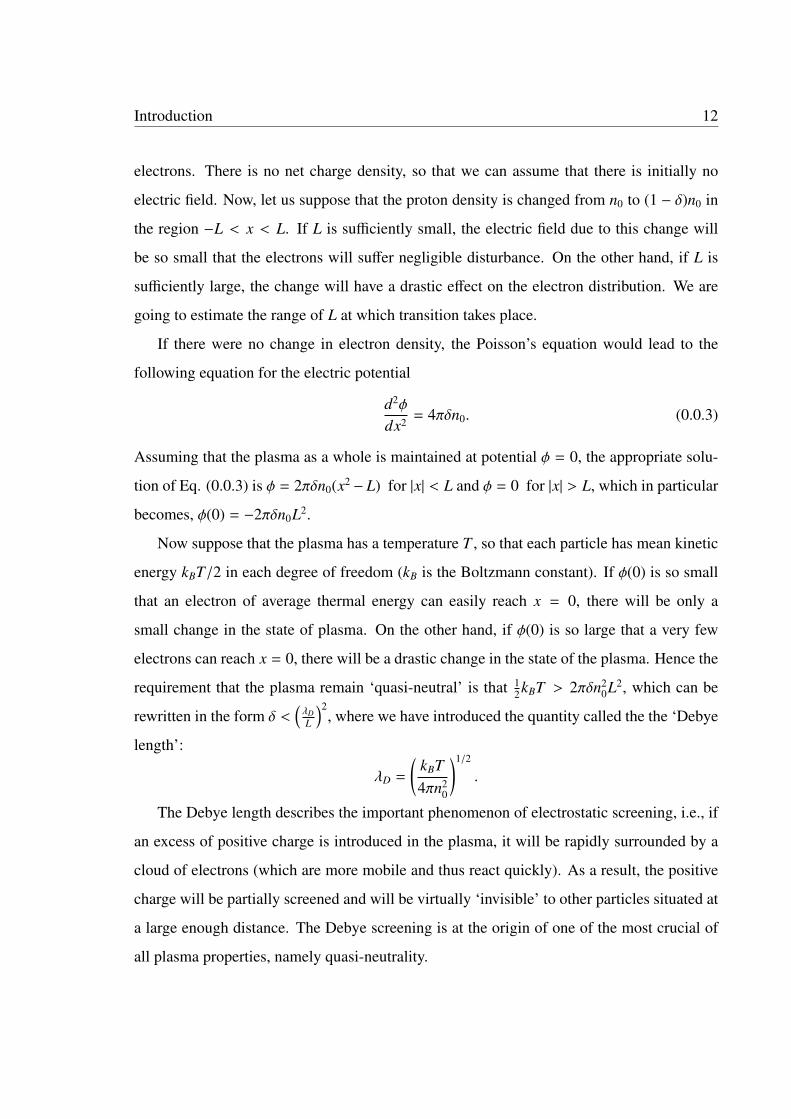
If there were no change in electron density, the Poisson’s equation would lead to the
following equation for the electric potential
d2φ
dx2 = 4πδn0. (0.0.3)
Assuming that the plasma as a whole is maintained at potential φ = 0, the appropriate solu-
tion of Eq. (0.0.3) is φ = 2πδn0(x2 − L) for |x| < L and φ = 0 for |x| > L, which in particular
becomes, φ(0) = −2πδn0L2.
Now suppose that the plasma has a temperature T , so that each particle has mean kinetic
energy kBT/2 in each degree of freedom (kB is the Boltzmann constant). If φ(0) is so small
that an electron of average thermal energy can easily reach x = 0, there will be only a
small change in the state of plasma. On the other hand, if φ(0) is so large that a very few
electrons can reach x = 0, there will be a drastic change in the state of the plasma. Hence the
requirement that the plasma remain ‘quasi-neutral’ is that 12kBT > 2πδn2
0L2, which can be
rewritten in the form δ <(λDL
)2, where we have introduced the quantity called the the ‘Debye
length’:
λD =
(kBT4πn2
0
)1/2
.
The Debye length describes the important phenomenon of electrostatic screening, i.e., if
an excess of positive charge is introduced in the plasma, it will be rapidly surrounded by a
cloud of electrons (which are more mobile and thus react quickly). As a result, the positive
charge will be partially screened and will be virtually ‘invisible’ to other particles situated at
a large enough distance. The Debye screening is at the origin of one of the most crucial of
all plasma properties, namely quasi-neutrality.

Introduction 13
A dimensionless parameter using the above quantities (me0, e, n0, and T ) exists, and it
reads as, coupling parameter i.e.,
Γc =4πe2n1/3
0
kBT. (0.0.4)
Γc can be written as the ratio of the potential energy to the average kinetic energy. When Γc
is small, the plasma is dominated by thermal effects. This is known as the weakly coupled
plasma. On the contrary, when Γc & 1, the plasma is said to be strongly coupled.
A violation of the local charge neutrality induces an electrostatic oscillation of the electric
field in the plasma with frequency ωp. This means that the quantity Tp = ωp/2π, called the
plasma period, estimates the characteristic time of charge separation.
Plasma can support ultra-high electric field which depends on the number density pertur-
bations according to the Poisson equation, ∇ · E = −4πen1, where n1 is the number density
perturbation. However, the maximum value of the field amplitude corresponds to a density
perturbation numerically equal to the unperturbed plasma density (i.e., n1 ∼ n0). It easily
leads to the Dawson limit given by Eq. (0.0.1).
However, plasmas can become relativistic when the temperature is very large (T > mc2)
[46] or in the presence of large amplitude waves [47]. The case of large amplitude wave for
cold plasma has been investigated by Akhiezer et al. [48]. In this case, relativistic corrections
to plasma particle’s mass and velocity are important.
Under the action of an oscillating field with large amplitude EM at frequency ω, the
plasma particle motion can be described in terms a parameter, called quiver velocity, i.e.,
ν = qEM/mωc, where q and m are the charge and mass of the particle. If ν 1, the
plasma particle motion is non relativistic. With the gradual increase of amplitude, plasma
particle velocity gradually become a significant fraction of light velocity, c. The condition
ν ≈ 1, corresponds to radiation intensity of the order of 1013−1016 W/cm2. Larger intensities
(& 1017 W/cm2) lead the plasma particles to be fully relativistic.

Introduction 14
Particle beam concept and beam parameters
There is no univocal definition of beam. Typically, a charged particle beam stands for a
collection of particles that have almost same same velocity and hence same kinetic energy
and, therefore, move in almost same direction. The charged particle beams we are dealing
with in this thesis are paraxial systems. In such a system the particle velocities are almost
oriented along a privileged direction, say z, called the propagation direction or longitudinal
direction. Let us denote by x and y a pair of orthogonal axis that are orthogonal to z, as well.
This way, x, y and z, consitute a Cartesian reference frame. In such a frame, the trajectory of
each beam particle can be represented by equation of the type:
z = z(x, y) . (0.0.5)
Then, the paraxial character of our beam is established by the conditions
dxdz 1 , and
dxdz 1 , (0.0.6)
which state that the slopes of the particle trajectories in the beam must be very small.
At normal temperature, the kinetic energies of the particles are higher than the thermal
energies. Charged particle beams can be categorized into two branches i.e., laminar beams
and nonlaminar beams. In a laminar beam, the particles follow fixed layers of trajectories
that never intersect. All the particles have identical transverse velocities and while flowing
they make a small angle with the propagation axis (paraxial motion). The area of the phase
space, that is occupied by a laminar beam, is a straight line of zero thickness. When the beam
crosses the ideal lens is transformed in a converging laminar beam. It is easy to transform a
diverging (or converging) beam to a parallel beam by using a lens of the proper focal length.
On the other hand, the particles of a nonlaminar beam have random transverse velocities.
Therefore, it is impossible to focus all particles from a location in the beam toward a common
point. Lenses can influence only the average motion of particles. The phase space plot of a
non-laminar beam is not a straight line.

Introduction 15
A charged particle beam can be released from a material source and propagated through
a medium (like plasma) or in a vacuum. When a charged particle beam has pulsed motion
in the longitudinal direction, it is called bunched beam. The unbunched (coasting) beam has
no pulses in the longitudinal direction. The bunched beams are the ones that are mostly used
in modern accelerators. Charged particle beams can be described by various properties viz.,
particle species, energy, current, beam size, beam emittance (a measure of thermal spreading
in the particle trajectories), brightness, etc.
The beam-plasma interaction ruled by the PWF mechanism can be described in various
situations those depend on the relative density of beam and plasma, the velocity, temperature,
collective or single particle behavior, etc. For instance, if the beam density is much smaller
than the plasma density i.e., nb n0, the system is in the overdense regime. When the beam
density is nearly equal or a little above the plasma density i.e., nb & n0 the PWF interaction
is in underdense regime [4–8].
Brief summary of all the chapters We report here the synthetic descrip-
tions of the chapters’ contents. To help the reader, they are also reported as abstracts at the
beginnings of each chapter.
Chapter 1: Models for plasmas
We present the basic concept of the kinetic theory for plasmas that are relevant for the self-
consistent plasma wake field excitation. We start from the Vlasov-Maxwell system of equa-
tions for a plasma. From the kinetic model of each plasma specie, we find the hierarchy of
moment equations of the distribution function that we truncate, with suitable closure condi-
tions, to the level of fluid theory. This way, the set of fluid Lorentz-Maxwell equations is
also presented in view of the construction of plasma wake field theory in Chapter 2. Finally,
a simple extension of both kinetic and fluid models to include collisional effects is presented.
Chapter 2: The theory of plasma wake field excitation: the Poisson-typeequation

Introduction 16
We present the general theory of plasma wake field excitation in a magnetoactive, nonrel-
ativistic, warm and collisionless plasma. This is done by using the 3D Lorentz-Maxwell
system of equation for the ‘beam-plasma’ system that has been presented in Chapter 1. The
driving beam is assumed to be ultra-relativistic in overdense regime. We first give a simple
concept of plasma wake field and plasma wake potential by starting from the expression of
the Lorentz force experienced by a test particle in its co-moving frame, in the presence of the
self-consistent EM field of the ‘beam-plasma’ system. Then, in the quasi-static approxima-
tion, we reduce the Lorentz-Maxwell system of equations to a novel 3D partial differential
equation, i.e., the generalized Poisson-type equation, that relates the beam density to the
wake potential. Such an equation extends the PWF theory to the case of warm plasmas
and accounts for the presence of an ambient magnetic field, the longitudinal and transverse
plasma pressure terms, and the generalized conditions of beam energy and sharpness of the
beam profile. The generalized Poisson-type equation found here is then specialized to sev-
eral limiting cases in order to recover the particular equations that have been used in the
literature.
Chapter 3: Models for charged particle beams and its self-consistent in-teraction with the surrounding medium
We formulate the kinetic description of an ultra-relativistic driving beam while self-consistently
interacting with the plasma wake field excited in a warm, magnetized, collisionless plasma
in overdense regime. The driver is supposed to be in the arbitrary conditions of sharpness
of its density profile. Such a general formulation is provided by starting from the relativistic
single-particle 3D Hamiltonian in the presence of an ambient magnetic field. In the reference
frame of the unperturbed particle, we express the Hamiltonian of the perturbed particle in
terms of a slight variation from the one of the unperturbed particle that is associated with the
relativistic unperturbed beam state. After expanding the four potential to the first-order and
performing the non-relativistic expansion with respect to the unperturbed state, we get the
effective single-particle Hamiltonian. The latter is used to construct the 3D Vlasov equation

Introduction 17
for the beam motion in the reference frame of the unperturbed particle. This way, by cou-
pling the Vlasov equation with the generalized Poisson-type equation obtained in Chapter 2,
we provide the self-consistent 3D kinetic description to be used in the next chapters to study
the self-modulated dynamics of the driver while interacting with the surrounding plasma.
Chapter 4: Transverse self-modulated beam dynamics of a nonlaminar,ultra-relativistic beam in a non relativistic cold plasma
An analysis of the self-modulated transverse dynamics of a cylindrically symmetric non-
laminar driving beam is carried out. To this end, we disregard the longitudinal dynamics.
Therefore, the general 3D Vlasov-Poisson-type system of equation constructed in Chapter
3 is reduced to a 2D pair of equations governing the spatiotemporal evolution of the purely
transverse dynamics of the driving beam, which is supposed to be very long compared to the
plasma wavelength and travelling through a cold, magnetized and overdense plasma. Due to
the conditions of very long beam, the self-consistent PWF mechanism is very efficient and it
sensitively characterizes the self-modulated dynamics.
The analysis is carried out by using the pair of Vlasov-Poisson-type equations in cylindri-
cal symmetry that are implemented by the virial equations to provide the analysis of the
self-modulated dynamics of the driver envelope. We show the important role played by the
constants of motions that are involved in such a description. We first carry out an analysis
in two different limiting cases, i.e., the local case (the beam spot size is much greater than
the plasma wavelength) and the strongly nonlocal case (the beam spot size is much smaller
than the plasma wavelength) where several types of self-modulation, in terms of focusing,
defocusing and betatron-like oscillations, are obtained and the criteria for instability, such
as collapse and self-modulation instability, are formulated. To this ends, within the context
of the envelope description, we find suitable envelope equations, i.e., ordinary differential
equations for the beam spot size, that are easily integrated analytically and that provide also
suitable physical explanations in terms of the method of the pseudo potential or Sagdeev
potential.

Introduction 18
Then, the analysis is extended to the case where the beam spot size and the plasma wave-
length are not necessarily constrained as in the local or strongly nonlocal cases. The analysis
of the system can be still carried out with the virial equations and with the same methods
used in the above limiting cases (envelope equations, Sagdeev potential) to provide a full
semi-analytical and numerical investigation for the envelope self-modulation. To this end,
criteria for predicting stability and self-modulation instability are suitably provided.
Chapter 5: Instability analysis of beam-plasma system
We carry out an analysis of the beam modes that are originated by perturbing the ‘beam-
plasma system’ in the purely longitudinal case. This is done by considering the pair of
3D Vlasov-Poisson-type equation, presented in Chapter 3 that are specialized to the case
in which the transverse driving beam dynamics is disregarded and only the longitudinal
dynamics becomes effective. To this end, we perturb the Vlasov-Poisson-type system up to
the first order, then take the Fourier transform to reduce the Vlasov-Poisson system to a set
of algebraic equations in the frequency and wavenumber domain, from which we easily get
a Landau-type dispersion relation for the beam modes, that is fully similar to the one holding
for plasma modes. First, we consider the case of a monochromatic beam (i.e., cold beam,
that is described by a distribution function in the form of delta-function in p space) for which
the existence of a purely growing mode is shown and a simple stability criterion formulated.
Then, by taking into account a unperturbed distribution function with finite, relatively small
width (small thermal correction), the Landau approach, widely used in other physics area,
leads to obtain both the dispersion relation for the real part (showing all the possible beam
modes in the diverse regions of the wavenumber) and an expression for the imaginary part of
the frequency (showing the stable or unstable character of the beam modes), which suggests
a simple stability criterion.
Chapter 6: The coupling impedance concept for PWF self-interaction
Starting from the collisionless Vlasov-Poisson-type system of equation for longitudinal beam
dynamics, that has been presented in Chapter 5, we formulate a novel approach in which

Introduction 19
we put forward the concept of longitudinal coupling impedance associated with the beam-
plasma interaction, in a way fully similar to the one in use in conventional particle accelerator
physics. As in the conventional theory, the concept of coupling impedance seems to be very
fruitful in a plasma-based accelerator to schematize the self-interaction of the relativistic
driving beam with the surrounding plasma. In particular, it allows us to develop a simple
instability analysis in the plane of the real and imaginary parts of the impedance that is based
on the Nyquist approach widely used in the control system theory. Furthermore, we extend
the Vlasov-Poisson-type system to the collision context with a simple model of collisions
between the plasma particles (actually plasma electrons) and the beam particles. Under these
assumptions, the role and the features of the coupling impedance defined here are compared
to then ones of the coupling impedance in conventional theory. Examples of specific physical
situations are finally illustrated.
Chapter 1
Models for plasmas
We present the basic concept of the kinetic theory for plasmas that are relevant for the self-consistent
plasma wake field excitation. We start from the Vlasov-Maxwell system of equations for a plasma.
From the kinetic model of each plasma specie, we find the hierarchy of moment equations of the
distribution function that we truncate, with suitable closure conditions, to the level of fluid theory.
This way, the set of fluid Lorentz-Maxwell equations is also presented in view of the construction of
plasma wake field theory in Chapter 2. Finally, a simple extension of both kinetic and fluid models to
include collisional effects is presented.
1.1 Preliminary considerations
We refer here to the notions of plasmas and charged particle beams (CPBs) given in the
Introduction. In both systems, the (charged) particles are free to move and their collective
dynamics is governed by the electromagnetic interactions. The most important difference
between plasmas and CPBs is that the former are globally neutral whilst the latter carry a
nonzero total electric charge. Since in this thesis we are interested in describing the self-
modulated dynamics of a beam, we consider the plasma as the environment which the beam
moves through and interacts with. Therefore, in the collective beam dynamics the role of the
plasma is taken into account through the wake fields produced therein. The wake fields can
be derived from a potential, i.e., the wake potential, which is a function of the Eulerian space
20

Models for plasmas 21
coordinates. The wake potential is related to the beam density by means of the Poisson-
like equation. This means that the beam interacts with the plasma through a macroscopic
quantity which can be indifferently provided by a kinetic or a fluid description. In this thesis,
we provide the Poisson-like equation within the context of the fluid plasma theory.
In the next section, in view of the presentation of the self-modulated dynamics of a rela-
tivistic beam travelling in a plasma (see Chapters 4-6), we will first present the simple kinetic
description of a nonrelativistic plasma, within the context of the Vlasov-Maxwell theory, and
derive the fluid limit and the corresponding set of plasma fluid equations (Lorentz-Maxwell
system). Then, we generalize the latter to the fluid theory of a relativistic plasma.
Plasma models depend on the adopted length scale. On a scale much less than λD, the
dynamics is governed by equations which take into account the collisions among the single
plasma particles (short range interaction). At this scale, the most appropriate description of
plasma is the microscopic one, which focuses on the single collision processes and on the
single-particle dynamics in the presence of microscopic electromagnetic fields. At length
scales of the order of λD, the short range interaction are almost negligible, whilst the sys-
tem dynamics is dominated by the longer range interactions. The latter are due to mean
macroscopic electric and magnetic fields. At such scales, the most appropriate description
of plasma is the one provided by the Boltzmann’s kinetic theory, but with the inclusions of
the collective effects due to the collective nature of the macroscopic fields. At length scales
much greater than λD, the plasma description reduces to the one of a set of fluids: a single
fluid for each ion specie and one for electrons. In this limiting case, the system dynamics
is governed by a set of fluid dynamics equations with the inclusion of the collective effects
introduced by the macroscopic fields.
The kinetic model for plasma has been first introduced by Vlasov [49]. The plasma
is thought to be as a system of macroparticles whose dimensions are of the order of λD.
They are assumed to be the effective particles of the system. Vlasov’s model is based on
the Hartree’s mean field theory [50] which allows to simplify the interaction among many
particles, by assuming that each particle moves in a field (mean field) generated by all the

Models for plasmas 22
other particles of the plasma. Note that the mean field depends on the instantaneous particle
distribution and it is defined in any point of the space. The kinetic model can be introduced
by means of the notion of single-particle Boltzmann’s phase space, also called reduced phase
space or simply µ-space [51]. A point P of this space represents a single-particle dynamical
state, i.e., the pair of single-particle position and velocity (or momentum). Therefore, P has
six coordinates: (r, v) = (x, y, z, vx, vy, vz), where r = (x, y, z) is the position of the generic
particle in configuration space and v = (vx, vy, vz) is the related velocity.
Let us now suppose to have a system of charged particles constituted by a so large number
of identical particles that, at the length scales of the order of the Debye length, the dynamical
states are distributed with continuity in µ-space. We define the Boltzmann’s distribution
function of such a system as the function f = f (r, v, t) such that the mean number, say dN, of
dynamical states within an elementary volume d3r d3v of the µ-space dN = f (r, v, t) d3r d3v.
Given the uniqueness of the solutions of the single-particle motion equations (provided that
the initial conditions are imposed), the above system is a set of identical but distinguishable
particles. Consequently, the dynamical states (i.e., points of the µ-space) are in a one-to-one
correspondence with the particle of the system. Then, at each instant of time t, the total
number of dynamical state concides with the total number, N, of system particles, i.e.,
N =
∫f (r, v, t) d3r d3v . (1.1.1)
Note that, if the particles keep their own identity during the evolution of the system (f.i.,
absence of ionization/recombination processes, decays, etc.), N remains unchanged in time.
It follows that f (r, v, t) is normalizable. Then, under this assumption, if we normalize f ,
i.e.,∫
f (r, v, t) d3r d3v = 1, it can be regarded as a probability density in µ-space. Adopting
the kinetic model, at the scale comparable to λD, it is then possible to describe any sys-
tem constituted by a large number of interacting charged particles, such as charged-particle
beams (usually produced and/or employed in an accelerating machine or naturally generated
in space and astrophysical environments) and plasmas (usually produced in and/or employed
in laboratory for a number of scientific and technological applications or already present in

Models for plasmas 23
space and astrophysical environments in the most diversified conditions of density and tem-
peratures). In particular, in a plasma we can attribute a distribution function, say fs(r, v, t), to
each species s, i.e., each subsystem of identical particles (called plasma components, such as
electrons and various species of ions). Let us assume that there are no processes capable to
change the identity of the particles of each specie and that the short-range collisions are neg-
ligible (collisionless plasma). Then, given the one-to-one correspondence between particles
and dynamical states, during the evolution of the system, the number of dynamical state of
a given specie that enter per unitary time an arbitrary volume of µ-space equals the number
of dynamical states of the same species that leave per unitary time the same volume. This
corresponds to assume an equation of continuity in µ-space for a continuous system of dy-
namical states of each species with density fs(r, v, t) and velocity field U(6) = (r, v) = (v, a),
where a is the instantaneous acceleration of the generic volume element of such a continuous
system. Then, we can write∂ fs
∂t+ ∇(6) ·
(fsU(6)
)= 0 , (1.1.2)
where ∇(6) = (∂x, ∂y, ∂z, ∂vx , ∂vy , ∂vz) is the six-dimensional gradient in the µ.
By taking into account that: (i) r and v are indipendent variables; (ii) given the force field
acting on the specie s, i.e., Fs = Fs(r, v, t), from the motion of the single particle (of mass
ms) it follows a = Fs(r, v, t)/ms; continuity equation (1.1.2) becomes
∂ fs
∂t+ v · ∇r fs +
Fs
ms· ∇v fs +
fs
ms(∇v · Fs) = 0 , (1.1.3)
where ∇r = (∂x, ∂y, ∂z) and ∇v = (∂vx , ∂vy , ∂vz) are the gradients in the configuration space and
in the velocity space, respectively. The force field Fs(r, v, t) can be in general the sum of the
external fields and the ones that are generated by the particles of the system (self-consistent
fields). For the time being, we confine our attention to the self-consistent fields and put:
Fs = qs[E + v × B], where the fields E = E(r, t) and B = B(r, t) satisfy suitable Maxwell’s
equations, whose sources are given by both the charge and current distributions ranging over
all the species. To calculate these source terms, we introduce the following macroscopic

Models for plasmas 24
quantities
ns(r, t) =
∫fs(r, v, t)d3v , (1.1.4)
Vs(r, t) =
∫v fs(r, v, t)d3v
ns, (1.1.5)
corresponding to the density and the mean velocity (also called current velocity or velocity
field) of the specie s, respectively. Then, the total charge and the total current of the specie s
are respectively given by
ρ =∑
s
qsns(r, t) , (1.1.6)
and
j =∑
s
qsns(r, t)Vs(r, t) , (1.1.7)
where qs is the charge of the single particle of the species s.
According to to above arguments and assumptions and observing that the electromagnetic
Lorentz force Fs satisfies the condition ∇v ·Fs = 0, from Eq. (1.1.3) and the above equations,
we obtain the following set of Vlasov-Maxwell system of equations, viz. (in cgs units),
∂ fs
∂t+ v · ∇r fs +
qs
ms[E + qv × B] · ∇v fs = 0 , (1.1.8)
∇ · E = 4πqs
∑s
∫fs(r, v, t)d3v , (1.1.9)
∇ · B = 0 , (1.1.10)
∇ × B =4πqs
c
∑s
∫v fs(r, v, t)d3v +
1c∂E∂t
, (1.1.11)
∇ × E = −1c∂ B∂t
, (1.1.12)
where s ranges over all particle species, which means all ions species and electrons and we
have used Eqs. (1.1.4) - (1.1.7). It describes the self-consistent spatiotemporal phase space
evolution of the plasma within the kinetic theory. It is worthy to outline some important
aspects of this system of equations.
1. For any s, Eq. (1.1.8) is called kinetic Vlasov equation for the specie s. It can be
thought as a Boltzmann equation in which the collisions are negligible. Actually, the
Models for plasmas 25
presence of long-range interaction through the Lorentz force term involves the self-
consistent collective effects and therefore makes this equation deeply different from
Boltzmann equation. For nstance, an important aspect of this diversity is the devel-
opment of non-dissipative damping of collective oscillations with reversible character,
usually referred to as the Landau damping. In the Vlasov’s kinetic theory, these pro-
cesses can be described as a statistical result of a large number of resonant interactions
between the collective modes and the individual particles of the plasma [52].
2. For any s, the left-hand side of Eq. (1.1.8) can be thought as the total derivative of fs.
In fact, we observe that:
∂ fs
∂t+ v · ∇r fs +
Fs
ms· ∇v fs =
∂ fs
∂t+ r · ∇r fs + v · ∇v fs =
d fs
dt.
Consequently, by virtu of Eq. (1.1.8), it follows that d fs/dt = 0. Hence, the distribu-
tion function fs is conserved along the characteristics r = r(t), v = v(t). This result
has the following simple physical interpretation. Since each fs represents the density
of dynamical states in µ-space, the set of these states constitutes an incompressible
fluid. Consequently, by virtu of the conservation of the number of dynamical states in
an arbitrary volume of µ-space (continuity equation), the volume of the phase space
associated with any subsystem of particles of the specie s conserves (Liouville theorem
in µ-space). It is easy to show that the same property holds for the volume associated
to any subsystem containing particles of all species.
3. The mathematical coupling among the equations of the system (1.1.8) - (1.1.12) corre-
sponds to the following representation of the self-consistency. In principle, given both
the initial conditions and the boundary conditions, we can formally integrate Vlasov
equation for each specie with respect to fs. Then we can compute both charge and
current distributions which, in turn, allow us to integrate the Maxwell equations for E
and B, once both initial and boundary conditions are imposed. However, to determine
explicitly fs for any s from Eq. (1.1.8), it is necessary to know already explicitly the
Models for plasmas 26
fields E and B; but, nevertheless, to determine the latter from the Maxwell equations it
is necessary to know explicitly the distributions of the sources (charges and currents)
and, therefore, fs for any s.
4. System of equations (1.1.8) - (1.1.12) is a system of nonlinear partial differential equa-
tions. The sources of nonlinearity lie in the third term at the left-hand side of Eq.
(1.1.8) for any s. The nonlinearity of system (1.1.8) - (1.1.12) makes impossible the
application of the superposition principle. Then, a linear combination of solutions of
system (1.1.8) - (1.1.12) is not, in turn, a solution of this system.
For simplicity, we will consider plasmas constituted by electrons and only one ion specie,
whose electric charge is e (i.e., atomic number Za = 1) which is the absolute value of the elec-
tron charge (the generalization to an arbitrary numbers of ion species with arbitrary atomic
number Za is not difficult), viz.,
∂ fe
∂t+ v · ∇r fe −
eme
[E + qv × B] · ∇v fe = 0 , (1.1.13)
∂ fi
∂t+ v · ∇r fi +
emi
[E + qv × B] · ∇v fi = 0 , (1.1.14)
∇ · E = 4πe[∫
fi(r, v, t) −∫
fe(r, v, t)], (1.1.15)
∇ · B = 0 , (1.1.16)
∇ × B =4πe
c
[∫v fi(r, v, t)d3v −
∫v fe(r, v, t)d3v
]+
1c∂E∂t
, (1.1.17)
∇ × E = −1c∂ B∂t
, (1.1.18)
where e and i stand for electrons and ions, respectively, and we have used Eqs. (1.1.4) -
(1.1.7).
1.2 Fluid theory of a nonrelativistic plasma:the Lorentz-Maxwell system
It is possible to derive a set of equations for fluid plasma species at scales much larger than
the Debye length for a certain species constituting the plasma. The set of Vlasov-Maxwell

Models for plasmas 27
equations can be cast into a set of fluid equations, called Lorentz-Maxwell (LM) system.
This can be done by reducing the system in µ- space to the configuration space. To do this,
we integrate Vlasov equation upon multiplying by appropriate monomial or polynomials of
velocity.
We first consider a plasma which is free from any external field. The plasma is constituted
by electrons and ions. Then, let us introduce the following differential operator in the µ-
space:
Ds =∂
∂t+ v · ∇r +
qs
ms
[E(r, t) +
vc× B(r, t)
]· ∇v .
In terms of this operator, Vlasov equation (1.1.8) can be written as,
Ds fs = 0 . (1.2.1)
Now we multiply Eq. (1.2.1) by a monomial of v, such as 1 (scalar), v (vector), vv (tensor),
..., and integrate over velocity space. Then, we perform the following integrals:∫Ds fs d3v = 0 , (1.2.2)∫
vDs fs d3v = 0 , (1.2.3)
........................... , (1.2.4)
by obtaining∂I(0)
s
∂t+ ∇r · I(1)
s = 0 , (1.2.5)
∂I(1)s
∂t+ ∇r · I(2)
s −qs
msI(0)
s
[E +
I(1)s
c× B
]= 0 , (1.2.6)
........................... , (1.2.7)
where we have introduced the following quantities: Moment of zero order of fs (scalar quan-
tity),
I(0)s =
∫fs(r, v, t) d3v = ns(r, t) . (1.2.8)
First order moment of fs (vector quantity, also called as current density of species s),
I(1)s =
∫v fs(r, v, t) d3v = ns(r, t)Vs(r, t) . (1.2.9)

Models for plasmas 28
Second order moment of fs (tensor quantity),
I(2)s =
∫vv fs(r, v, t) d3v =
Ps
ms= ns〈vv〉s , (1.2.10)
........................... . (1.2.11)
In Eqs. (1.2.8) - (1.2.11), the integration is done over all the entire velocity space. In addition,
flux momentum density tensor of the species s is,
Ps ≡ ms I(2)s (r, t) = ms
∫vv fs(v) d3v = msns
∫vv fs(r, v, t) d3v∫
fs(r, v, t) d3v. (1.2.12)
From Eq. (1.2.5), we can observe that to know the zero-order moment, I(0)s , we need to know
the first order moment I(1)s . Furthermore, from Eq. (1.2.6), we can observe that to know the
first-order moment, I(1)s , we need to know the second-order moment I(2)
s . Similarly, we can
obtain an equation for second-order moment, which will contain third-order moment as well.
In fact, an evolution equation for the moment of order n would contain the moments of order
n + 1.
To obtain fluid equations up to the first order of moment equation, we need to truncate
the hierarchy by expressing I(2)s in terms of moments of lower order (closure reports). This
can be done by taking averages of physical quantities on scales much greater than λD which
represents a sort of smoothing operation. If λ is the characteristic length of the spatial varia-
tion of the physical quantities involved in our description, then the condition of validity of a
fluid model is expressed by λD λ. For each specie s, we express velocity v as the sum of
a part corresponding to its average and another part which has a random character, i.e.,
v = Vs + u , (1.2.13)
where Vs = 〈v〉s and 〈u〉s = 0. Here, u is the random velocity of the particle that takes into
account their thermal motion. Using Eqs. (1.1.4) and (1.1.5), into Eqs. (1.2.8) - (1.2.11) and
(1.2.13), Eqs. (1.2.5) and (1.2.6) become,
∂ns
∂t+ ∇r · (nsVs) = 0 , (1.2.14)
∂Vs
∂t+ (Vs · ∇r)Vs =
qs
ms
(E +
Vs
c× B
)−∇r · ps
msns, (1.2.15)

Models for plasmas 29
where ps is the pressure tensor on the species s, defined as
ps = msns〈uu〉s = ms
∫fs uu d3u . (1.2.16)
Since the short ranged collisions are considered negligible and if no other form of dissipa-
tions are important, then we can assume the following isotropic form for the pressure tensor
ps = psI , (1.2.17)
where I is the identity tensor and ps is the scalar pressure of the species s. It is also assumed
to be ps = nskBTs for temperatures Ts and Boltzmann constant kB. The most recurrent forms
of closure of the system are the following one corresponds to the adiabatic hypothesis, i.e.,
Ts/nγsr−1s = constant, where γsr is the ratio of specific heat at constant pressure to the specific
heat at constant volume of species s. In this case, Eq. (1.2.15) becomes:(∂
∂t+ Vs · ∇r
)Vs =
qs
ms
(E +
Vs
c× B
)− γsr
kBTs
ms
∇rns
ns. (1.2.18)
The other hypothesis is called isothermal, i.e., ∇rTs = 0, for which case Eq. (1.2.15) can be
written as (∂
∂t+ Vs · ∇r
)Vs =
qs
ms
(E +
Vs
c× B
)−
kBTs
ms
∇rnns
. (1.2.19)
Equations (1.2.18) and (1.2.14) or (1.2.19) and (1.2.14) have to be coupled with the Maxwells
equations given in the following form:
∇ · E = 4π∑
s
qsns , (1.2.20)
∇ · B = 0 , (1.2.21)
∇ × B =4πc
∑s
qsnsVs +1c∂E∂t
, (1.2.22)
∇ × E = −1c∂ B∂t
. (1.2.23)
The system of equations consisting of (1.2.20) - (1.2.23), (1.2.14) and (1.2.18) is known as
the Lorentz-Maxwell system in the adiabatic approximation, whilst the system of equations

Models for plasmas 30
(1.2.20) - (1.2.23), (1.2.14) and (1.2.19) is known as Lorentz-Maxwell system in the isother-
mal approximation, respectively. Note that these systems of equations contain the following
sources of nonlinearity:
1. the product nsVs in continuity equation and equation for ∇ × B;
2. the products (Vs · ∇) Vs and Vs × B, and the term Ts∇ns/ns in motion equation.
1.3 Kinetic description of a relativistic plasma
The Vlasov-Maxwell system of Eqs. (1.1.8) - (1.1.12) can be easily generalized to a rela-
tivistic case [53, 54].
Let us consider a collisionless plasma with an arbitrary different species of particles,
where a particle of species s has rest mass mso. The plasma is assumed to be relativistic, i.e.,
its particles may move at relativistic speed. This implies that, in principle, particle masses
depend on the speed (note that the relativistic mass is ms = msoγ, γ = 1/(1 − v2/c2)1/2 be-
ing the relativistic factor) and, therefore, the Boltzmann µ-space, presented above for the
non-relativistic case, has to be redefined. In fact, the pair (r, v) cannot be used to denote
a dynamical state. If p is the instantaneous single-particle linear momentum, the µ-space
is now defined as the six-dimensional space of all the pairs (r,p). Each pair (r,p) repre-
sents a dynamical state of the single particle. Given the uniqueness of the relativistic motion
equations, the set of dynamical states associated to each species is in a one-to-one corre-
spondence with the particles of the same specie. Therefore, each species is described by a
particle density fs = fs(r, v, t). As in the non-relativistic case, the particles interact by the
electromagnetic forces they create themselves so that the density functions fs together with
the self consistent electromagnetic fields E(r, t) and B(r, t) evolve according to the following

Models for plasmas 31
relativistic Vlasov-Maxwell system, viz.,
∂ fs
∂t+ v · ∇r fs + qs
(E +
vc× B
)· ∇p fs = 0 , (1.3.1)
∇ · E = 4π∑
s
qs
∫fs(r,p, t)d3 p , (1.3.2)
∇ · B = 0 , (1.3.3)
∇ × B =4πc
∑s
qs
∫v fs(r,p, t)d3 p +
1c∂E∂t
, (1.3.4)
∇ × E = −1c∂ B∂t
, (1.3.5)
where s ranges over all the species and the particle velocity is given by
v =p
ms0γ=
p
ms0
(1 + p2/m2
s0c2)1/2 . (1.3.6)
Note that the number density ns, the current velocity Vs, the total charge density ρ and the
total current densities j are here defined, respectively, as
ns(r, t) =
∫fs(r,p, t)d3 p , (1.3.7)
Vs(r, t) =
∫v fs(r,p, t)d3 p
ns, (1.3.8)
ρ(r, t) =∑
s
qsns(r, t) =∑
s
qs
∫fs(r,p, t)d3 p , (1.3.9)
j(r, t) =∑
s
qsns(r, t)Vs(r, t) =∑
s
qs
∫v fs(r,p, t)d3 p . (1.3.10)
It is easy to see that the relativistic extension of the Vlasov-Maxwell system (1.1.13) -
(1.1.18) is the following
∂ fe
∂t+ v · ∇r fe − e
(E +
vc× B
)· ∇p fe = 0 , (1.3.11)
∂ fi
∂t+ v · ∇r fi + e
(E +
vc× B
)· ∇p fi = 0 , (1.3.12)

Models for plasmas 32
∇ · E = 4πe[∫
fi(r,p, t)d3 p −∫
fe(r,p, t)d3 p], (1.3.13)
∇ · B = 0 , (1.3.14)
∇ × B =4πe
c
[∫v fi(r,p, t)d3 p −
∫v fe(r,p, t)d3 p
]+
1c∂E∂t
, (1.3.15)
∇ × E = −1c∂ B∂t
, (1.3.16)
where s = e (electrons), i (ions).
1.4 Fluid description of a relativistic plasma
The procedure of constructing the hierarchy of moment equations, starting from the Vlasov-
Maxwell system (1.1.8) - (1.1.12), can be easily extended to the relativistic case to obtain
the Lorentz-Maxwell system of equation for a relativistic plasma [52, 53]. We easily arrive
to the following relativistic Lorentz-Maxwell fluid equations
∂ns
∂t+ ∇ · (nsVs) = 0 , (1.4.1)(
∂
∂t+ Vs · ∇
)Ps = qs
(E +
Vs
c× B
)− ∇ · Πs , (1.4.2)
∇ × E = −1c∂B∂t
, (1.4.3)
∇ × B = −4πc
∑s
qsns Vs +1c∂E∂t
, (1.4.4)
∇ · E = 4π∑
s
qsns , (1.4.5)
∇ · B = 0 , (1.4.6)
where ns = ns(r, t) and Vs = Vs(r, t) are the number density and the fluid velocity of the s-th
specie and still defined by Eqs. (1.3.7) and (1.3.8), Πs(r, t) is a stress tensor accounting for
the thermal effects of the s-th specie, Πs is the pressure tensor and
Ps(r, t) = ms0γs(r, t)Vs(r, t) (1.4.7)

Models for plasmas 33
is the relativistic fluid linear momentum of the s-th specie, γs(r, t) being the fluid relativistic
factor of the s-th specie, i.e.,
γs(r, t) =1√
1 − V2s (r, t)/c2
. (1.4.8)
The stress tensor term, under the assumptions of adiabatic or isothermal conditions, can be
cast in forms that are similar to the corresponding non relativistic cases, respectively.
Note that the relativistic Lorentz-Maxwell system contains all the sources of nonlinearity
that are contained in the corresponding non-relativistic system, but in addition it contains the
one due to the relativistic mass variation through the term ms0Vs/√
1 − V2s (r, t)/c2 in motion
equation.
1.5 Collisional plasmas
The descriptions provided in the previous sections has regarded collisionless plasmas. This is
a physical circumstance compatible with the Vlasov equation, which can be basically thought
as a sort of collisionless Boltzmann equation. Although the presence of collective effects in
Vlasov equations make this equation quite different from Boltzmann equation, actually one
can introduce collision effects in the plasma by assuming that the right-hand side of Vlasov
equation is no longer zero, but equal to a source of collisions, as it is done with Boltzmann
equation in the case of a neutral gas [51]. Therefore, the existence of non negligible colli-
sional effects of the specie s makes non zero the total derivative of the distribution function fs
along the characteristics. This, in turn, implies the non conservation of the volume in the µ-
space (i.e., Liouville theorem for the s-th specie is no longer valid). It is worthy noting that,
if we include the collision source terms in the Vlasov-Maxwell system, the corresponding
fluid model will contain collisional terms, as well. Then, in both kinetic and fluid models,
they lead to the inclusion of the dissipative effects as well as the macroscopic irreversibility
of the system.
We assume here that: (i) the rate of collisions among particles belonging to the same

Models for plasmas 34
specie is much less than the characteristic parameter of time variation of the plasma quan-
tities; (ii) the rate of binary collisions between particles of different species is comparable
to the characteristic parameter of time variation of the plasma quantities. Then, a possible
estimate of the variation rate of fs due to binary collisions of the particles of s-th specie with
the ones of the s′-th specie is given by(∂ fs
∂t
)coll,ss′
=fs′ − fs
τss′, (1.5.1)
where τss′ is the characteristic time of the momentum transfer from the specie s-th to the
specie s′. Consequently, the total rate that accounts for all the collisional contributions is
obtained by summing over all the species s′ , s. Therefore, the total derivative is no longer
zero, as in the collisionless case, but
d fs
dt=
∑s′
(∂ fs
∂t
)coll,ss′
=∑
s′
fs′ − fs
τss′. (1.5.2)
Hence, the inclusion of the collisions in Eq. (1.3.1) finally gives
∂ fs
∂t+ v · ∇r fs + qs
(E +
vc× B
)· ∇p fs =
∑s′
fs′ − fs
τss′. (1.5.3)
For any s, Eq. (1.5.3) has to be coupled with Eqs. (1.3.2) - (1.3.5).
To get the corresponding fluid description, we have to calculate the moments of Eq.
(1.5.3). We easily see that the zero-th order moment equation gives still the continuity Eq.
(1.4.1), because the integral of the collision term at the right-hand side of Eq. (1.5.3) over
all the momentum space vanishes in the absence of production or losses of particles of each
specie. Moreover, the first-order moment equation gives the motion equation of the s-th
specie that in principle differs from Eq. (1.4.2) due to the presence of the variation of the
momentum of the specie s per unit time due to the collisions with all the other species. Under
the assumption that the current velocities of two different species, say s and s′, are different,
a net momentum transfer between them takes place. It turns out that such a momentum
transfer is proportional to the difference of current velocities of the two different species.
Therefore, the total net momentum transfer of the s-th specie results from the sum over all
Models for plasmas 35
the species s′ which appears as a new term at the right-hand side of the motion equation, i.e.,(∂
∂t+ Vs · ∇
)Ps = qs
(E −
Vs
c× B
)− ∇ · Πs =
∑s′
Vs′ − Vs
τss′. (1.5.4)
1.6 Conclusions
The basic concept of the kinetic theory for plasmas that are relevant for the self-consistent
plasma wake field excitation have been presented. Starting from the Vlasov-Maxwell system
of equations for the single plasma specie, we have provided the kinetic description of the
plasma. Furthermore, we have found the hierarchy of moment equations of the single-specie
distribution function that we have truncated, with suitable closure conditions, to the level of
fluid theory. In view of the construction of plasma wake field theory in Chapter 2, this has
allowed to provide the fluid description of the plasma in terms of the set of fluid Lorentz-
Maxwell system of equations. Finally, both kinetic and fluid models have been also extended
in order to include simple collisional effects.

Chapter 2
The theory of plasma wake fieldexcitation: the Poisson-type equation
We present the general theory of plasma wake field excitation in a magnetoactive, nonrelativistic,
warm and collisionless plasma. This is done by using the 3D Lorentz-Maxwell system of equation
for the ‘beam-plasma’ system, where the sources of the EM fields include charges and currents of
both plasma and beam. The driving beam is assumed to be relativistic in overdense regime. We
first give a simple concept of plasma wake field and plasma wake potential by starting from the
expression of the Lorentz force experienced by a test particle in its co-moving frame, in the presence
of the self-consistent EM field of the ‘beam-plasma’ system. Then, in the quasi-static approximation,
we reduce the Lorentz-Maxwell system of equations to a novel 3D partial differential equation, i.e.,
the generalized Poisson-type equation, that relates the beam density to the wake potential. Such an
equation extends the PWF theory to the case of warm plasmas and accounts for the presence of an
ambient magnetic field, the longitudinal and transverse plasma pressure terms, and the generalized
conditions of beam energy and sharpness of the beam profile. The generalized Poisson-type equation
found here is then specialized to several limiting cases in order to recover the particular equations
that have been used in the literature.
36

The models of plasma wake field excitation... 37
2.1 Introduction
The basic concept of PWF can be suitably provided by determining the force experienced by
a relativistic particle of charge q, which has a relative motion with respect to an electromag-
netic field, i.e., the pair (E(r, t),B(r, t)) of electric and magnetic field that has been created
by some source.
Let us denote the test particle velocity by v and assume that it has the relativistic motion
along z, i.e., v = βcz + v⊥, where β ∼ 1 and v⊥ is the transverse component of v such that
v⊥ c. Then, the Lorentz force experienced by the particle is:
F =dpdt
= q[E +
vc× B
], (2.1.1)
where p is the linear momentum of the particle, i.e.,
p = m0γ v , (2.1.2)
where m0 and γ are the rest mass and relativistic factor, respectively. We now introduce the
four-potential (A(r, t), φ(r, t)), such that:
E = −∇φ −1c∂A∂t
, (2.1.3)
B = ∇ × A . (2.1.4)
Then, Eq. (2.1.1) can be easily cast as:
F = q[∇
(A ·
vc− φ
)−
1c
(∂
∂t+ v · ∇
)A]. (2.1.5)
Note that vector and scalar potentials, i.e., A and φ, depend on the Eulerian coordinates r
and t, whilst F depends on r, v and t, v being independent of r. We split r, gradient operator,
and A into longitudinal and transverse components, i.e.,
r = zz + r⊥ , (2.1.6)
∇ = z∂
∂z+ ∇⊥ , (2.1.7)
A = zAz + A⊥ . (2.1.8)

The models of plasma wake field excitation... 38
Then, Eq. (2.1.5) becomes:
F = q∇ (βAz − φ) + q∇(A⊥ ·
v⊥c
)−
qc
(∂
∂t+ βc
∂
∂z
)A −
qc
(v⊥ · ∇⊥) A , (2.1.9)
which under the following coordinate transformation
ξ(r⊥, z, t) = z − β′ct , (2.1.10)
R⊥(r⊥, z, t) = r⊥ , (2.1.11)
τ(r⊥, z, t) = t , (2.1.12)
where β′ ∼ 1, becomes:
F′ = q∇′Ω + q(β′ − β)∂A′
∂ξ−
qc∂A′
∂τ+ q∇′
(A′⊥ ·
v′⊥c
)− q
(v′⊥c· ∇′⊥
)A′ . (2.1.13)
Here we have denoted the transformed quantities by primes and also defined the quantity
Ω(R⊥, ξ, τ) = βA′z(R⊥, ξ, τ) − φ′(R⊥, ξ, τ). We assume that the test particle and the fields
are moving at the same speed, i.e., β′ = β (rigidity condition). Furthermore, since v′⊥ c,
we neglect the higher-order terms coming from the last two terms at right hand side of Eq.
(2.1.13). Then, we finally obtain:
F′(R⊥, ξ, τ) = q∇′Ω(R⊥, ξ, τ) −qc∂A′(R⊥, ξ, τ)
∂τ, (2.1.14)
where ∇′ = ∂/∂R⊥ + z∂/∂ξ.
2.2 Definition of plasma wake field
Let us now consider a relativistic charged particle beam moving through a plasma along
the z-direction. We assume that the beam has a finite temperature. Therefore, we assume
that the beam particles experience the effect of the thermal spreading while moving in the
plasma along z in such a way that the beam performs a nonlaminar motion. In these physical
conditions, the velocity of each beam particle can be thought as the sum of a determinis-
tic part corresponding to the relativistic motion along z whose average is not zero (mean

The models of plasma wake field excitation... 39
velocity), plus a random instantaneous part along an arbitrary direction whose average is
zero corresponding to the thermal spreading. In addition, we assume that the beam temper-
ature corresponds to a non-relativistic random motion, so that the instantaneous slope of the
single-particle trajectory can be considered sufficiently small to fulfill the conditions:
dxdz 1 ,
dydz 1 , (2.2.1)
where x and y are the transverse space coordinates assumed by the single particles. Condition
(2.2.1) is equivalent to assume that the beam is paraxial.
The excess of charge that is introduced by the beam while moving through the plasma
is responsible for the violation of the local charge neutrality, which in turn, creates a local
electric field in the system. On the other hand, the motion of the beam corresponds to a
current injected in the plasma which generates a local magnetic field. We can conclude
that the propagation of a relativistic charged particle beam through the plasma perturbs the
initial stationary conditions of the plasma itself. Therefore, the beam-plasma system excites
therein the local electromagnetic field. This is a macroscopic field, whose sources are the
charges and the currents of both plasma and beam, that it is called plasma wake field (PWF).
The corresponding mechanism is usually referred to as PWF excitation. Since the PWF is
excited the propagation of the relativistic beam through the plasma, it is evident that it moves
through the plasma with almost the same velocity of the beam itself.
Note that, in principle, the PWF can act on any test particle which is instantaneously
in the plasma region where it has been excited. We want here to emphasize the causality
aspects of the beam-plasma interaction: (i) starting from the initial stationary condition,
the charged particle beam propagates through the plasma and introduces therein an excess
of charge and an external current; (ii) the latter generates plasma perturbations that, in turn,
excite the PWF. Then, we can conclude that the relativistic beam has actually driven the PWF
excitation by means of the an active medium, i.e., the plasma. We call this beam the driving
beam or simply the driver of the PWF excitation. In other words, the mechanism of the PWF
excitation is obtained by the external action of the driver into the active medium which, in

The models of plasma wake field excitation... 40
turn, can sustain such an excitation. Although the causality works as described here, the
connection between the external action of the driver and the response of the active medium
manifests so rapidly that they should be considered contextually, i.e., on same timescale.
If the driver is actually a bunch, i.e., it carries a very sharp particle distribution in con-
figuration space (number density), the PWF acts on test particles those are behind the bunch
travelling at almost its same speed. If the driver density profile has a 3D character it is
expected that the PWF has a 3D character as well. Therefore, a test particle can be accel-
erated or decelerated by the instantaneous longitudinal component of the PWF, depending
on the synchronism conditions of the test particles with respect to the phase of the PWF. On
the other hand, meanwhile, the transverse component of the PWF may affect the test particle
motion by providing a transverse manipulation of its trajectory, such as focusing, defocusing,
etc.
If the driver is a sufficiently long beam, the PWF will act also on the particle of the driver
itself, providing this way a sort of self-interaction of the beam: the driver is affected by the
PWF that itself has generated.
According to the above assumptions, the force produced by the PWF, that is experienced
by a test charged particle located in the position (R⊥, ξ) at time τ, is given by Eq. (2.1.14).
However, since the external action of the driver and the plasma-response manifest on the
same timescale, we can assume that ∂/∂τ ' 0 (quasi-static approximation). Consequently,
the force per unitary charge, at the location (r⊥, ξ) that is generated by the PWF mechanism
is given by:
W(r⊥, ξ) = ∇Ω(r⊥, ξ) , (2.2.2)
where ∇ = ∂/∂r⊥+z∂/∂ξ and Ω(r⊥, ξ) = βAz(r⊥, ξ)−φ(r⊥, ξ), Az(r⊥, ξ) and φ(r⊥, ξ) being the
z-component of the vector potential and scalar potential, respectively, of the beam-plasma
system at location (r⊥, ξ). Here, W is the PWF excited by the driving beam and Ω is the
related plasma wake potential. It can be easily proven that
∇⊥Wz =∂W⊥
∂ξ, (2.2.3)

The models of plasma wake field excitation... 41
which is the Panofsky-Wenzel theorem [55]. Here Wz and W⊥ are longitudinal and trans-
verse components of W, respectively. Therefore, in the quasi-static approximation, W has
the feature of an electrostatic field which can be derived by an effective potential Ω. In the
subsequence sections, we show that the Lorentz-Maxwell system that governs, at the diverse
physical conditions, the spatiotemporal evolution of the plasma in the presence of both in-
ternal sources (charge and current provided by the plasma) and external sources (charge and
current provided by the beam), can be reduced to a Poisson-type equation which relates the
PWF potential to the beam density.
All the Poisson-type equation that we will obtain at the diverse physical assumptions,
can be cast in the following generic form:
PΩ = Q nb , (2.2.4)
where nb = nb(r⊥, ξ) is the local number density of the beam; P and Q are two generic partial
differential operators whose explicit form depends on the physical assumptions we take for
the beam-plasma system. Their role will be crucial in Chapter 4 and subsequent chapters,
where we couple Eq. (2.2.4) with appropriate equations for the beam dynamics to describe
the self-consistent spatio-temporal beam evolution (beam self-modulation).
2.3 Lorentz-Maxwell system of equations for thebeam-plasma system
Let us consider a plasma where a relativistic charged particle beam is travelling through,
along the z axis, as the driver of the PWF. We also assume, for simplicity, that the plasma
consists of electrons and a single specie of ions with Za = 1. The latter are also supposed
to be infinitely massive forming a uniform background of positive charge with unperturbed
number density n0. Let us finally assume that the plasma electrons have in general a rela-
tivistic motion. Then, according to the section 1.4 and 1.5, and in order to take into account
the presence of an external uniform magnetic field and collisions between plasma particles
and the beam particles, our system is described by the following set of coupled relativistic

The models of plasma wake field excitation... 42
fluid equations (s = e):
∂ne
∂t+ ∇ · (neVe) = 0 , (2.3.1)(
∂
∂t+ Ve · ∇
)Pe = −e
[E +
Ve
c× B
]− ∇ · Πe −
(Ve − Vb)τeb
, (2.3.2)
∇ × E = −1c∂B∂t
, (2.3.3)
∇ × B = −4πc
ene Ve +4πc
qnb Vb +1c∂E∂t
, (2.3.4)
∇ · E = 4πe (n0 − ne) + 4πqnb , (2.3.5)
∇ · B = 0 , (2.3.6)
where Ve = Ve(r, t) is the electron plasma current velocity, Pe = Pe(r, t) is the electron
plasma fluid linear momentum, i.e.,
Pe(r, t) = me0γe(r, t)Ve(r, t) (2.3.7)
(me0 being the plasma electron rest mass), Πe = Πe(r, t) is the pressure tensor of the electron
plasma fluid, Vb = Vb(r, t) is the beam fluid velocity, ne = ne(r, t) and nb = nb(r, t) are
the electron plasma number density and the beam number density, respectively, and q is the
charge of the single particle of the beam. In addition, within the adiabatic approximation,
we assume that the pressure tensor has the form:
Πe =
pe⊥ 0 0
0 pe⊥ 0
0 0 pez
, (2.3.8)
where pe⊥ = nekBTe⊥, and pez = nekBTez, Te⊥ and Tez being transverse and longitudinal
temperatures, respectively. Here, pe⊥ and pez are transverse and longitudinal pressures, re-
spectively. The adiabatic approximation implies that the following conditions:
pe⊥n−Γe⊥e = constant (2.3.9)
and
pezn−Γeze = constant (2.3.10)

The models of plasma wake field excitation... 43
has to be satisfied. Here Γe⊥ = D + 2/D = 2 and Γez = D + 2/D = 3 are the adiabatic ex-
ponents in transverse and longitudinal directions, respectively, where D is the number of de-
grees of freedom. Note that, in the above set of fluid equations, the driving charged-particle
beam is involved through its charge density, i.e., ρb(r, t) ≡ qnb(r, t), its current density,
i.e., Jb(r, t) ≡ qnb(r, t)Vb(r, t), and the collision term accounting for the collisions between
plasma electrons and beam particles, i.e., − (Ve − Vb) /τeb, τeb being the corresponding char-
acteristic collision time.
In the next sections, confining our attention to a collisionless nonrelativistic plasma, we shall
reduce the system (2.3.1) - (2.3.10) to suitable Poisson-type equations for the diverse physi-
cal assumptions we shall adopt. To this end, we assume that density and fluid velocity of the
driver are, respectively, of the form:
nb(r, t) = nb(r⊥, ξ) , (2.3.11)
Vb(r, t) = z βc + vb(r⊥, ξ) , (2.3.12)
where ξ = z − βct and vb is a fluid component such that: |vb| c, with β ∼ 1. Equation
(2.3.12) states that the driver’s velocity is basically relativistic along with a 3D nonrelativistic
instantaneous displacement, vb, with instantaneous orientation, that accounts for both the
longitudinal and transverse beam dynamics.
2.4 Poisson-type equation in overdense regime: collision-less nonrelativistic plasma
We assume that the driver has the maximum density, say nbmax, much smaller than the unper-
turbed plasma density, i.e.,
nbmax n0 . (2.4.1)
This condition defines the so-called overdense regime. It implies that the driver introduces
a small perturbation in terms of charge density and current density into the plasma. Let
us assume that initially the plasma is in the following equilibrium state: ne = n0, Ve = 0,
The models of plasma wake field excitation... 44
E = 0, B = B0 = B0z = constant, and Πe = Π0 = constant. Here B0 is a uniform and
constant magnetic field which is oriented along the longitudinal direction. It is evident that
it represents an external magnetic field. Once the driver is supposed to travel through the
plasma, the resulting excited PWF is a quantity of the order of nb/n0. According to the
assumption of overdense regime, this ratio is much smaller than 1. Therefore, it is clear
that the driver density nb is a first-order quantity and produces first-order displacement in all
physical quantities. So that, it is possible to linearize the system of Eqs. (2.3.1) - (2.3.10)
with the additional assumptions (2.3.11) and (2.3.12) and assume that the plasma motion is
nonrelativistic, i.e., Pe(r, t) ≈ me0Ve(r, t).
In order to find the appropriate Poisson-type equation for the system under consideration,
we do the following steps.
(i) We express both electric and magnetic fields, E and B, in terms of the four-potential
(A, φ), according to Eqs. (2.1.3) and (2.1.4) and adopt the Lorentz gauge, i.e.,
∇ · A +1c∂φ
∂t= 0 . (2.4.2)
(ii) We linearize the system of Eqs. (2.3.1) - (2.3.12). To this end, we introduce first-
order perturbations of all the physical quantities (denoted by the subscript 1) around the
above mentioned equilibrium states, i.e., ne = n0 + n1, Ve = V1, E = E1, B = B0 + B1,
A = A0 + A1, φ = φ1, and Π = Π0 + Π1. Consequently, the Lorentz-Maxwell system of
equations becomes,
∂n1
∂t+ n0∇ · V1 = 0, (2.4.3)
∂V1
∂t=
eme0
[∇φ1 +
1c∂A1
∂t
]−
eB0
me0 cV1 × z −
∇ · Π1
me0 n0, (2.4.4)
1c2
∂2φ1
∂t2 − ∇2φ1 = 4π
[qnb − en1
], (2.4.5)
1c2
∂2A1
∂t2 − ∇2A1 =
4πc
(qnbβcz − en0V1) , (2.4.6)

The models of plasma wake field excitation... 45
where Eqs. (2.1.3) and (2.1.4) become,
E1 = −∇φ1 −1c∂A1
∂t, (2.4.7)
B0 + B1 = ∇ × A0 + ∇ × A1 . (2.4.8)
Here, A0 denotes the zero-order vector potential, i.e., B0 = ∇ × A0(r). Note that A0(r) =
(B0 × r) /2 . Correspondingly, the Lorentz gauge can be split into the following conditions:
∇ · A0 = 0, (2.4.9)
∇ · A1 +1c∂φ1
∂t= 0. (2.4.10)
(iii) We split the vector quantities and the gradient operator (∇) into perpendicular (de-
noted by the subscript⊥) and longitudinal components (denoted by the subscript z), i.e., Eqs.
(2.4.3) - (2.4.6) give:
∂n1
∂t+ n0
∂V1z
∂z+ n0∇⊥ · V1⊥ = 0, (2.4.11)
∂V1z
∂t=
eme0
(∂φ1
∂z+
1c∂A1z
∂t
)−
ΓzkBT0z
me0n0
∂n1
∂z, (2.4.12)
∂V1⊥
∂t=
eme0
(∇⊥φ1 +
1c∂A1⊥
∂t
)+ ωc(V1⊥ × z) −
Γ⊥kBT0⊥
me0n0∇⊥n1, (2.4.13)
1c2
∂2φ1
∂t2 −∂2φ
∂z2 − ∇2⊥φ1 = 4π
[qnb − en1
], (2.4.14)
1c2
∂2A1z
∂t2 −∂2A1z
∂z2 − ∇2⊥A1z =
4πc
(qnbβc − en0V1z) , (2.4.15)
1c2
∂2A1⊥
∂t2 −∂2A1⊥
∂z2 − ∇2⊥A1⊥ = −
4πen0
cV1⊥, (2.4.16)
where ωc = −eB0/me0c is the electron cyclotron frequency.
(iv) We perform the coordinate transformation:
ξ = z − βct , r′⊥ = r⊥ , τ = t . (2.4.17)
Consequently,
∂/∂z = ∂/∂ξ , ∇⊥ = ∇′⊥ , ∂/∂t = −βc∂/∂ξ + ∂/∂τ , (2.4.18)
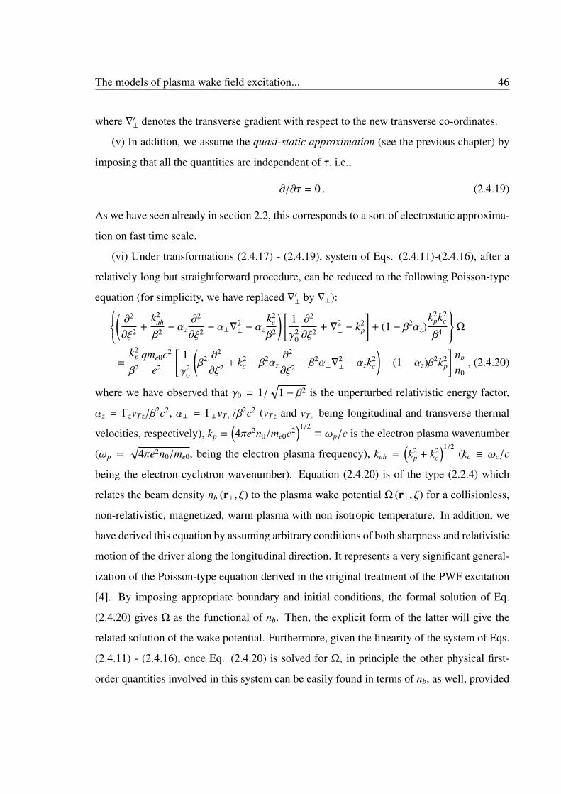
The models of plasma wake field excitation... 46
where ∇′⊥ denotes the transverse gradient with respect to the new transverse co-ordinates.
(v) In addition, we assume the quasi-static approximation (see the previous chapter) by
imposing that all the quantities are independent of τ, i.e.,
∂/∂τ = 0 . (2.4.19)
As we have seen already in section 2.2, this corresponds to a sort of electrostatic approxima-
tion on fast time scale.
(vi) Under transformations (2.4.17) - (2.4.19), system of Eqs. (2.4.11)-(2.4.16), after a
relatively long but straightforward procedure, can be reduced to the following Poisson-type
equation (for simplicity, we have replaced ∇′⊥ by ∇⊥):(∂2
∂ξ2 +k2
uh
β2 − αz∂2
∂ξ2 − α⊥∇2⊥ − αz
k2c
β2
) [1γ2
0
∂2
∂ξ2 + ∇2⊥ − k2
p
]+ (1 − β2αz)
k2pk2
c
β4
Ω
=k2
p
β2
qme0c2
e2
[1γ2
0
(β2 ∂
2
∂ξ2 + k2c − β
2αz∂2
∂ξ2 − β2α⊥∇
2⊥ − αzk2
c
)− (1 − αz)β2k2
p
]nb
n0, (2.4.20)
where we have observed that γ0 = 1/√
1 − β2 is the unperturbed relativistic energy factor,
αz = ΓzvTz/β2c2, α⊥ = Γ⊥vT⊥/β
2c2 (vTz and vT⊥ being longitudinal and transverse thermal
velocities, respectively), kp =(4πe2n0/me0c2
)1/2≡ ωp/c is the electron plasma wavenumber
(ωp =√
4πe2n0/me0, being the electron plasma frequency), kuh =(k2
p + k2c
)1/2(kc ≡ ωc/c
being the electron cyclotron wavenumber). Equation (2.4.20) is of the type (2.2.4) which
relates the beam density nb (r⊥, ξ) to the plasma wake potential Ω (r⊥, ξ) for a collisionless,
non-relativistic, magnetized, warm plasma with non isotropic temperature. In addition, we
have derived this equation by assuming arbitrary conditions of both sharpness and relativistic
motion of the driver along the longitudinal direction. It represents a very significant general-
ization of the Poisson-type equation derived in the original treatment of the PWF excitation
[4]. By imposing appropriate boundary and initial conditions, the formal solution of Eq.
(2.4.20) gives Ω as the functional of nb. Then, the explicit form of the latter will give the
related solution of the wake potential. Furthermore, given the linearity of the system of Eqs.
(2.4.11) - (2.4.16), once Eq. (2.4.20) is solved for Ω, in principle the other physical first-
order quantities involved in this system can be easily found in terms of nb, as well, provided
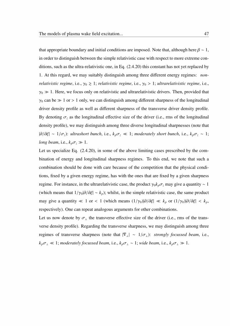
The models of plasma wake field excitation... 47
that appropriate boundary and initial conditions are imposed. Note that, although here β ∼ 1,
in order to distinguish between the simple relativistic case with respect to more extreme con-
ditions, such as the ultra-relativistic one, in Eq. (2.4.20) this constant has not yet replaced by
1. At this regard, we may suitably distinguish among three different energy regimes: non-
relativistic regime, i.e., γ0 & 1; relativistic regime, i.e., γ0 > 1; ultrarelativistic regime, i.e.,
γ0 1. Here, we focus only on relativistic and ultrarelativistic drivers. Then, provided that
γ0 can be 1 or > 1 only, we can distinguish among different sharpness of the longitudinal
driver density profile as well as different sharpness of the transverse driver density profile.
By denoting σz as the longitudinal effective size of the driver (i.e., rms of the longitudinal
density profile), we may distinguish among three diverse longitudinal sharpnesses (note that
|∂/∂ξ| ∼ 1/σz): ultrashort bunch, i.e., kpσz 1; moderately short bunch, i.e., kpσz ∼ 1;
long beam, i.e., kpσz 1.
Let us specialize Eq. (2.4.20), in some of the above limiting cases prescribed by the com-
bination of energy and longitudinal sharpness regimes. To this end, we note that such a
combination should be done with care because of the competition that the physical condi-
tions, fixed by a given energy regime, has with the ones that are fixed by a given sharpness
regime. For instance, in the ultrarelativistic case, the product γ0kpσz may give a quantity ∼ 1
(which means that 1/γ0|∂/∂ξ| ∼ kp); whilst, in the simple relativistic case, the same product
may give a quantity 1 or < 1 (which means (1/γ0)|∂/∂ξ| kp or (1/γ0)|∂/∂ξ| < kp,
respectively). One can repeat analogous arguments for other combinations.
Let us now denote by σ⊥ the transverse effective size of the driver (i.e., rms of the trans-
verse density profile). Regarding the transverse sharpness, we may distinguish among three
regimes of transverse sharpness (note that |∇⊥| ∼ 1/σ⊥): strongly focussed beam, i.e.,
kpσ⊥ 1; moderately focussed beam, i.e., kpσ⊥ ∼ 1; wide beam, i.e., kpσ⊥ 1.

The models of plasma wake field excitation... 48
2.5 Ultrarelativistic driver in a cold plasma: longitudinalsharpness regimes
We assume that the driver is ultra-relativistic. This means that the condition γ0 1, implies
that in Eq. (2.4.20) we can surely replace β with 1. Furthermore, the cold plasma assumption
implies that αz = α⊥ = 0. In this framework we consider two cases: strongly magnetized
and unmagnetized cases.
2.5.1 Magnetized plasma
The strongly magnetized plasma assumption stands for the condition kc & kp. The latter
means that the effect of the external magnetic field, i.e., B0, in terms of gyromotion has to
be at least comparable to the collective plasma motion. Given the present technology to
produce magnetic field amplitudes up to tens of tesla, in laboratory we may have at most
kc . kp. However, in the astrophysical environments, B0 can assume values such that also
the condition kc kp can be easily fulfilled.
Ultrashort bunch
According to the arguments presented in the previous sections, the assumptions taken here
allow us to reduce Eq. (2.4.20) to the following:[(∂2
∂ξ2 + k2uh
) (1γ2
0
∂2
∂ξ2 + ∇2⊥ − k2
p
)+ k2
pk2c
]Ω = k2
pqme0c2
e2
[1γ2
0
(∂2
∂ξ2 + k2c
)− k2
p
]nb
n0, (2.5.1)
which is based on the very delicate interplay between the longitudinal strong sharpness and
the extreme relativistic energy conditions. They compensate each other, in such a way to
ensure that the term (1/γ0) |∂/∂ξ| is non negligible.
Moderately short bunch
Excluding the extreme astrophysical magnetized plasma conditions, if the driver is simply a
moderately short bunch, Eq. (2.4.20) reduces to:[(∂2
∂ξ2 + k2uh
) (∇2⊥ − k2
p
)+ k2
pk2c
]Ω = −k4
pqme0c2
e2
nb
n0, (2.5.2)

The models of plasma wake field excitation... 49
where the sharpness no longer compensates the effect of the extreme energy conditions.
Equation (2.5.2) has been derived for the first time in Ref. [56].
Long beam
When the beam length is long enough to fulfill the condition kpσz 1, then the second-order
derivative with respect to ξ in Eq. (2.5.2) can be neglected and, it simplifies as:(∇2⊥ − k2
p
)+
k2pk2
c
k2uh
Ω = −k4
p
k2uh
qme0c2
e2
nb
n0, (2.5.3)
which has been used in [56] to investigate the PWF excitation in quantum regime. Note that
now the longitudinal coordinate ξ appears only as parameter in Eq. (2.5.3). As we will see
better later, it can be used as one of the governing equation of the purely transverse dynamics
of a paraxial nonlaminar beam, provided that ξ plays the role of a timelike variable.
2.5.2 Unmagnetized plasma
If the ambient magnetic field is absent or its effects can be considered negligible, in Eq.
(2.4.20) we can impose the condition B0 = 0 which corresponds to put kc = 0. Then, the
various cases of longitudinal sharpness are straightforwardly obtaine as follows.
Ultrashort bunch
According to the arguments presented in the previous sections, the assumptions taken here
allow us to reduce Eq. (2.5.1) to the following:(∂2
∂ξ2 + k2p
) (1γ2
0
∂2
∂ξ2 + ∇2⊥ − k2
p
)Ω = k2
pqme0c2
e2
[1γ2
0
∂2
∂ξ2 − k2p
]nb
n0. (2.5.4)
Also Eq. (2.5.4) is based on the very delicate interplay between the longitudinal strong
sharpness and the extreme relativistic energy conditions, in such a way they compensate
each other to ensure that the term (1/γ0) |∂/∂ξ| is non negligible. Note that Eq. (2.5.4) has
been derived in a recent work where it was used to investigate the formation and stability of
a hollow electron beam in the presence of a PWF excitation driven by an ultra-short electron
bunch in a unmagnetized cold plasma [57].

The models of plasma wake field excitation... 50
Moderately short bunch
Once the condition, kc = 0, is imposed, Eq. (2.5.2) reduces to:(∂2
∂ξ2 + k2p
) (∇2⊥ − k2
p
)Ω = −k4
pqme0c2
e2
nb
n0, (2.5.5)
which is equivalent, in case of electrons/positron beams, to the set of equations that has been
derived for the first time in Ref. [4].
Long beam
By substituting kc = 0 in Eq. (2.5.2), we obtain:
(∇2⊥ − k2
p
)Ω = −k2
pqme0c2
e2
nb
n0, (2.5.6)
which has been recently used to investigate the self-modulated transverse dynamics in both
classical [58–60] and quantum-like [61, 62] domains. Note that, as in the magnetized case,
also here the longitudinal coordinate ξ appears only as parameter.
2.6 Ultrarelativistic driver in a cold plasma: transverse sharp-ness regimes
Similarly to the previous section, we specialize Eq. (2.4.20) for the diverse cases of trans-
verse sharpness that can be obtained in combination with the ultrarelativistic regime of a
driver travelling in a cold plasma (αz = α⊥ = 0). Also here we consider the two cases of a
strongly magnetized and unmagnetized plasma, respectively.
2.6.1 Magnetized plasma
Strongly focussed beam
According to the classification presented in the previous section, the strongly focussed beam
assumption corresponds to the condition kpσ⊥ 1. Therefore, by imposing it in Eq. (2.4.20)

The models of plasma wake field excitation... 51
we easily obtain:[(∂2
∂ξ2 + k2uh
) (1γ2
0
∂2
∂ξ2 + ∇2⊥
)+ k2
p k2c
]Ω = k2
pqme0c2
e2
[1γ2
0
(∂2
∂ξ2 + k2c
)− k2
p
]nb
n0. (2.6.1)
Here, the derivatives with respect to ξ are not affected by any approximation, because the
longitudinal sharpness is considered to be arbitrary (therefore to be specified for each specific
case).
Moderately focussed beam
In this case, since kpσ⊥ ∼ 1, it is obvious that in Eq. (2.4.20) we have just to put: αz = α⊥ =
0, and no comparison between transverse and longitudinal sharpness is assumed in special
cases. Then, the corresponding expression coincides with Eq. (2.5.1).
Wide beam
When the beam is wide enough to fulfill the condition kpσ⊥ 1, then Eq. (2.4.20) can be
reduced as the following:[(∂2
∂ξ2 + k2uh
) (1γ2
0
∂2
∂ξ2 − k2p
)+ k2
pk2c
]Ω = k2
pqme0c2
e2
[1γ2
0
(∂2
∂ξ2 + k2c
)− k2
p
]nb
n0. (2.6.2)
2.6.2 Unmagnetized plasma
If the ambient magnetic field is absent or its effects can be considered negligible, in Eq.
(2.4.20) we put kc = 0. Then, the various cases of longitudinal sharpness are straightfor-
wardly obtained as follows.
Strongly focussed beam
When the condition kc = 0 is replaced in Eq. (2.6.1), we easily obtain the following Poisson-
type equation: (∂2
∂ξ2 + k2p
) (1γ2
0
∂2
∂ξ2 + ∇2⊥
)Ω = k2
pqme0c2
e2
(1γ2
0
∂2
∂ξ2 − k2p
)nb
n0. (2.6.3)

The models of plasma wake field excitation... 52
Moderately focussed beam
Once the condition kc = 0 is imposed, Eq. (2.5.1) reduces to:(∂2
∂ξ2 + k2p
) (1γ2
0
∂2
∂ξ2 + ∇2⊥ − k2
p
)Ω = k2
pqme0c2
e2
(1γ2
0
∂2
∂ξ2 − k2p
)nb
n0, (2.6.4)
which is equivalent, in case of electrons/positron beams, to the set of equations that has been
derived for the first time in Ref. [4].
Wide beam
By substituting ∇⊥ = 0 in Eq. (2.5.4), we obtain:(∂2
∂ξ2 + k2p
) (1γ2
0
∂2
∂ξ2 − k2p
)Ω = k2
pqme0c2
e2
(1γ2
0
∂2
∂ξ2 − k2p
)nb
n0. (2.6.5)
2.7 Poisson-type equation for purely longitudinal case
We can also confine our attention on 1D case of purely longitudinal beam profile. In this
case, in Eq. (2.4.20), all the transverse derivative should be suppressed while retaining the
longitudinal ones.
2.7.1 Magnetized plasma
Warm plasma
By putting α⊥ = 0 and ∇⊥ = 0, we easily get:[(∂2
∂ξ2 + k2uh − αz
∂2
∂ξ2 − αzk2c
) (1γ2
0
∂2
∂ξ2 − k2p
)+ (1 − αz)k2
pk2c
]Ω
= k2pqme0c2
e2
[1γ2
0
(∂2
∂ξ2 + k2c − αz
∂2
∂ξ2 − αzk2c
)− (1 − αz)k2
p
]nb
n0. (2.7.1)
Cold plasma
If in addition we put αz = 0, we have the Poisson-type equation for the case of cold plasma,[(∂2
∂ξ2 + k2uh
) (1γ2
0
∂2
∂ξ2 − k2p
)+ k2
pk2c
]Ω = k2
pqme0c2
e2
[1γ2
0
(∂2
∂ξ2 + k2c
)− k2
p
]nb
n0. (2.7.2)

The models of plasma wake field excitation... 53
2.7.2 Unmagnetized plasma
Warm plasma
By putting α⊥ = ∇⊥ = kc = 0, we easily get:(∂2
∂ξ2 + k2p − αz
∂2
∂ξ2
) (1γ2
0
∂2
∂ξ2 − k2p
)Ω =
k2p qme0c2
e2
[1γ2
0
(∂2
∂ξ2 − αz∂2
∂ξ2
)− (1 − αz)k2
p
]nb
n0.
(2.7.3)
Cold plasma
If in addition we put αz = 0, we have the Poisson-type equation for the case of cold plasma,(∂2
∂ξ2 + k2p
) (1γ2
0
∂2
∂ξ2 − k2p
)Ω = k2
pqme0c2
e2
[1γ2
0
∂2
∂ξ2 − k2p
]nb
n0. (2.7.4)
If 1/γ0∂/∂ξ kp, then above equation becomes(∂2
∂ξ2 + k2p
)Ω = k2
pqme0c2
e2
nb
n0. (2.7.5)
2.8 Poisson-type equation for purely transverse case
Now we confine our attention on 2D case of purely transverse beam profile. In Eq. (2.4.20)
all the longitudinal derivative should be suppressed while retaining the transverse ones.
2.8.1 Magnetized plasma
Warm plasma
By putting αz = 0 = ∂/∂ξ = 0, we easily get:[(k2
uh − α⊥∇2⊥
) (∇2⊥ − k2
p
)+ k2
pk2c
]Ω = k2
pqme0c2
e2
[1γ2
0
(k2
c − α⊥∇2⊥
)− k2
p
]nb
n0. (2.8.1)
Cold plasma
If in addition we put α⊥ = 0, we have the Poisson-type equation for the case of cold plasma,(∇2⊥ − k2
p
)+
k2pk2
c
k2uh
Ω =k2
p
k2uh
qme0c2
e2
(k2
c
γ20
− k2p
)nb
n0. (2.8.2)

The models of plasma wake field excitation... 54
2.8.2 Unmagnetized plasma
Warm plasma
By putting αz = ∂/∂ξ = kc = 0, we easily find:(k2
p − α⊥∇2⊥
) (∇2⊥ − k2
p
)Ω = −k2
pqme0c2
e2
(1γ2
0
α⊥∇2⊥ + k2
p
)nb
n0. (2.8.3)
Cold plasma
If in addition we put α⊥ = 0, we have the Poisson-type equation for the case of cold plasma,(∇2⊥ − k2
p
)Ω = −k2
pqme0c2
e2
nb
n0. (2.8.4)
2.9 Conclusions
We have presented the general theory of plasma wake field excitation in a magnetoactive,
nonrelativistic, warm, overdense, and collisionless plasma. This has been accomplished by
using the set of 3D fluid equations, comprising continuity and the motion equations, that
are coupled with the Maxwell equations (i.e., Lorentz-Maxwell system) in the adiabatic
approximation (see Chapter 1), in the presence of an ultra-relativistic driving beam. We
have first put forward the simple concept of plasma wake field and plasma wake potential
by starting from the expression of the Lorentz force experienced by a test particle, in its co-
moving frame, in the presence of the self-consistent EM field provided by the ‘beam-plasma’
system. In the quasi-static approximation, we have reduced the above Lorentz-Maxwell
system to a novel 3D partial differential equation, called here the generalized Poisson-type
equation. It relates the beam density to the wake potential and extends the PWF theory to
the case of warm plasmas. Additionally, it accounts for the presence of an ambient magnetic
field, the longitudinal and transverse plasma pressure terms, and the generalized conditions
of beam energy and sharpness of the beam profile. We have finally specialized this novel
equation to several limiting cases in order to recover the particular equations that have been
used in the literature.

Chapter 3
Models for charged particle beams andits self-consistent interaction with thesurrounding medium
We formulate the kinetic description of an relativistic driving beam while self-consistently interacting
with the plasma wake field excited in a warm, magnetized, collisionless plasma in overdense regime.
The driver is supposed to be in the arbitrary conditions of sharpness of its density profile. Such a
general formulation is provided by starting from the relativistic single-particle 3D Hamiltonian in
the presence of an ambient magnetic field. In the reference frame of the unperturbed particle, we
express the Hamiltonian of the perturbed particle in terms of a slight variation from the one of the
unperturbed particle that is associated with the relativistic unperturbed beam state. After expanding
the four potential to the first-order and performing the non-relativistic expansion with respect to the
unperturbed state, we get the effective single-particle Hamiltonian. The latter is used to construct
the 3D Vlasov equation for the beam motion in the reference frame of the unperturbed particle. This
way, by coupling the Vlasov equation with the generalized Poisson-type equation obtained in Chapter
2, we provide the self-consistent 3D kinetic description to be used in the next chapters to study the
self-modulated dynamics of the driver while interacting with the surrounding plasma.
55
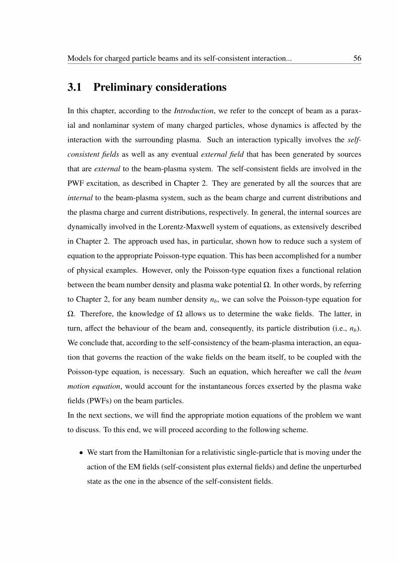
Models for charged particle beams and its self-consistent interaction... 56
3.1 Preliminary considerations
In this chapter, according to the Introduction, we refer to the concept of beam as a parax-
ial and nonlaminar system of many charged particles, whose dynamics is affected by the
interaction with the surrounding plasma. Such an interaction typically involves the self-
consistent fields as well as any eventual external field that has been generated by sources
that are external to the beam-plasma system. The self-consistent fields are involved in the
PWF excitation, as described in Chapter 2. They are generated by all the sources that are
internal to the beam-plasma system, such as the beam charge and current distributions and
the plasma charge and current distributions, respectively. In general, the internal sources are
dynamically involved in the Lorentz-Maxwell system of equations, as extensively described
in Chapter 2. The approach used has, in particular, shown how to reduce such a system of
equation to the appropriate Poisson-type equation. This has been accomplished for a number
of physical examples. However, only the Poisson-type equation fixes a functional relation
between the beam number density and plasma wake potential Ω. In other words, by referring
to Chapter 2, for any beam number density nb, we can solve the Poisson-type equation for
Ω. Therefore, the knowledge of Ω allows us to determine the wake fields. The latter, in
turn, affect the behaviour of the beam and, consequently, its particle distribution (i.e., nb).
We conclude that, according to the self-consistency of the beam-plasma interaction, an equa-
tion that governs the reaction of the wake fields on the beam itself, to be coupled with the
Poisson-type equation, is necessary. Such an equation, which hereafter we call the beam
motion equation, would account for the instantaneous forces exserted by the plasma wake
fields (PWFs) on the beam particles.
In the next sections, we will find the appropriate motion equations of the problem we want
to discuss. To this end, we will proceed according to the following scheme.
• We start from the Hamiltonian for a relativistic single-particle that is moving under the
action of the EM fields (self-consistent plus external fields) and define the unperturbed
state as the one in the absence of the self-consistent fields.

Models for charged particle beams and its self-consistent interaction... 57
• We split the vector quantities in longitudinal (parallel to the beam propagation direc-
tion) and radial (perpendicular to the beam propagation direction) components.
• We perturb the physical quantities around the unperturbed state.
• We finally find the effective Hamiltonian associated with the single-particle motion in
the beam co-moving frame.
3.2 Relativistic Hamiltonian for a single-particle motion inthe presence of EM fields
Let us consider a relativistic charged particle of charge q and rest mass mb0, moving with an
arbitrary velocity v in the presence of an EM field, i.e., E = E(r, t), B = B(r, t). It is well
known that the Hamiltonian for such a motion is given by [63]:
H(r,P, t) = c[(
P −qc
A)2
+ m2b0c2
]1/2
+ qφ , (3.2.1)
where A = A(r, t) and φ = φ(r, t) are vector and scalar potential, respectively, that are
associated with the fields E(r, t) and B(r, t) by means of the relations (2.1.3) and (2.1.4),
respectively. In Eq. (3.2.1), P is the canonical momentum which is related to the particle
kinetic linear momentum, p = mb0γv, by:
P = mb0γv +qc
A , (3.2.2)
where γ =(1 − v2/c2
)−1/2is the relativistic gamma factor.
In the absence of the fields, i.e., E = B = 0, we can define the unperturbed state of the
particle, i.e., v = v0 ≡ βcz (β ∼ 1) and γ = γ0 ≡ (1 − β2)−1/2, in which the particle trajectory
is a straight line that we have assumed to be the z− axis.
Note that the state of the particle remains unperturbed also if we consider the presence of
an uniform and constant magnetic field B0 = B0z, oriented along the z− axis. In fact, since
the particle velocity in this state, i.e., v = v0, is constant of motion and has the longitudinal
component only, the particle does not interact with B0 and therefore, does not assume a

Models for charged particle beams and its self-consistent interaction... 58
transverse component during the time. Therefore, it is easy to see that the Hamiltonian
associated with such an unperturbed state is:
H0 = mb0γ0c2 . (3.2.3)
3.2.1 Slightly perturbed motion
If we now consider a paraxial relativistic charged-particle travelling along the z− axis in the
presence of the same uniform and constant magnetic field B0, we can state that each beam
particle has an instantaneous velocity that can be cast in the following form:
v = βcz + u , (3.2.4)
where u represents slight displacement of v from the unperturbed state v0 = βcz, i.e.,
u c , (3.2.5)
with an arbitrary instantaneous orientation. Therefore, taking into account all the possible
slight displacements that are possible in a paraxial beam, the unperturbed state particle plays
the role of an ideal condition of the beam particle. Note that the perturbed state requires
the presence of an EM field, whose strengths have to be compatible with Eq. (3.2.4) and
condition (3.2.5). Note also that the quantity u has in general longitudinal and transverse
components, i.e.,
u = uzz + u⊥ . (3.2.6)
3.2.2 Perturbed effective single particle Hamiltonian
We perturb all the physical quantities of our interest around the state of the unperturbed
particle, i.e.,
γ = γ0 + γ1 , (3.2.7)
P = P0 +P = mb0γ0βc z +Pz z +P⊥ , (3.2.8)
A = A1zz + A0⊥ + A1⊥ , (3.2.9)
φ = φ1 , (3.2.10)
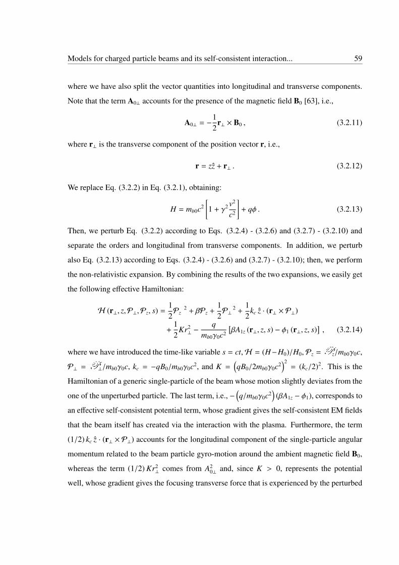
Models for charged particle beams and its self-consistent interaction... 59
where we have also split the vector quantities into longitudinal and transverse components.
Note that the term A0⊥ accounts for the presence of the magnetic field B0 [63], i.e.,
A0⊥ = −12
r⊥ × B0 , (3.2.11)
where r⊥ is the transverse component of the position vector r, i.e.,
r = zz + r⊥ . (3.2.12)
We replace Eq. (3.2.2) in Eq. (3.2.1), obtaining:
H = mb0c2[1 + γ2 v2
c2
]+ qφ . (3.2.13)
Then, we perturb Eq. (3.2.2) according to Eqs. (3.2.4) - (3.2.6) and (3.2.7) - (3.2.10) and
separate the orders and longitudinal from transverse components. In addition, we perturb
also Eq. (3.2.13) according to Eqs. (3.2.4) - (3.2.6) and (3.2.7) - (3.2.10); then, we perform
the non-relativistic expansion. By combining the results of the two expansions, we easily get
the following effective Hamiltonian:
H (r⊥, z,P⊥,Pz, s) =12Pz
2 + βPz +12P⊥
2 +12
kc z · (r⊥ × P⊥)
+12
Kr2⊥ −
qmb0γ0c2
[βA1z (r⊥, z, s) − φ1 (r⊥, z, s)
], (3.2.14)
where we have introduced the time-like variable s = ct,H = (H−H0)/H0, Pz =Pz/mb0γ0c,
P⊥ = P⊥/mb0γ0c, kc = −qB0/mb0γ0c2, and K =(qB0/2mb0γ0c2
)2= (kc/2)2. This is the
Hamiltonian of a generic single-particle of the beam whose motion slightly deviates from the
one of the unperturbed particle. The last term, i.e., −(q/mb0γ0c2
)(βA1z − φ1), corresponds to
an effective self-consistent potential term, whose gradient gives the self-consistent EM fields
that the beam itself has created via the interaction with the plasma. Furthermore, the term
(1/2) kc z · (r⊥ × P⊥) accounts for the longitudinal component of the single-particle angular
momentum related to the beam particle gyro-motion around the ambient magnetic field B0,
whereas the term (1/2) Kr2⊥ comes from A2
0⊥ and, since K > 0, represents the potential
well, whose gradient gives the focusing transverse force that is experienced by the perturbed
Models for charged particle beams and its self-consistent interaction... 60
single-particle in the presence of B0.
Let us now consider the coordinate transformation; ξ = z−β′
s, R⊥ = r⊥, τ = s, P′
z = Pz +α,
and P′
⊥ = P⊥, where α is an arbitrary real constant. Its inverse is; z = ξ + β′
τ, r⊥ = R⊥,
s = τ, Pz = P′
z − α, and P⊥ = P′
⊥. In addition, we write the Hamilton equations associated
with Hamiltonian 3.2.14, i.e.,
dzds
=∂H
∂Pz= Pz + β, , (3.2.15)
dPz
ds= −
∂H
∂z=∂
∂z
q
mb0γ0c2
[βA1z (r⊥, z, s) + φ1 (r⊥, z, s)
]. (3.2.16)
Then, by using above mentioned transformations, Eqs. (3.2.15) and (3.2.16) can be easily
reduced to
dξdτ
= P′
z +(β − β
′)− α ≡
∂H
∂P′z, (3.2.17)
dP′
z
dτ=
∂
∂ξ
[q
mb0γ0c2
(βA
′
1z − φ′
1
)]≡ −
∂H
∂ξ, (3.2.18)
where A′
1z = A′
1z (R⊥, ξ, τ), φ′
1 = φ′
1 (R⊥, ξ, τ) andH =H(R⊥, ξ,P
′
⊥,P′
z, τ)
stand for the
image of A1z (r⊥, z, s), φ1 (r⊥, z, s) andH , respectively, under the transformations.
If we now require that the above transformation leads to dξ/dτ = P′
z, we get that α = β− β′
.
Consequently, Eq. (3.2.17) becomes:
dξdτ
= P′
z ≡∂H
∂P′z. (3.2.19)
If, in addition, we impose the rigidity condition, i.e., β′
= β, which means that our refer-
ence frame corresponds to the one where the unperturbed particle is at rest, the fourth of
transformations becomes simply
P′
z = Pz , (3.2.20)
and the effective potential Ω (R⊥, ξ, τ) =[βA
′
1z (R⊥, ξ, τ) − φ′
1 (R⊥, ξ, τ)]
becomes the plasmawake potential that has been introduced in Chapter 2. Furthermore, Eqs. (3.2.20), (3.2.19)and (3.2.18) allow us finally to get easily the transformed Hamiltonian, viz.,
H (R⊥, ξ,P⊥,Pz, τ) =12Pz
2 +12P⊥
2 +12
kc z · (R⊥ × P⊥) +12
KR2⊥ + Uw (R⊥, ξ, τ) , (3.2.21)

Models for charged particle beams and its self-consistent interaction... 61
where we have introduced the dimensionless plasma wake potential energy:
Uw (R⊥, ξ, τ) = −q Ω (R⊥, ξ, τ)
mb0γ0c2 . (3.2.22)
3.3 The Vlasov equation for a relativistic charged-particlebeam
In this section, we find the kinetic equation that describes the phase space evolution of the
perturbed charged particles, whose Hamiltonian is given by Eq. (3.2.21), that belong to
a relativistic paraxial beam. To this end, we first of all introduce the six-dimensional µ-
space, i.e., (R⊥, ξ,P⊥,Pz). Then, we denote by f = f (R⊥, ξ,P⊥,Pz, τ) the single-particle
distribution function in such a phase space. According to Chapter 1, the kinetic equation is
given by the total derivative of f , viz.,
∂ f∂τ
+dξdτ
∂ f∂ξ
+dR⊥dτ·∂ f∂R⊥
+dPz
dτ∂ f∂Pz
+∂P⊥∂τ·∂ f∂P⊥
= 0 . (3.3.1)
By substituting Eq. (3.2.21) in Eq. (3.3.1), we easily get the following Vlasov equation:
∂ f∂τ
+Pz∂ f∂ξ
+
[P⊥ +
12
kc (z × R⊥)]·∂ f∂R⊥
−∂Uw
∂ξ
∂ f∂Pz
−
[KR⊥ −
12
kc (z × P⊥) +∂Uw
∂R⊥
]·∂ f∂P⊥
= 0 ,
(3.3.2)
which describes the collective behavior of the charged-particle beam while interacting
with the plasma via the plasma wake potential and in the presence of an ambient mag-
netic field. It is worthy noting that, if N is the total number of particles in the beam,
−mb0γ0c2 z∂Uw (R⊥, ξ, τ) /∂ξ and −mb0γ0c2 ∂Uw (R⊥, ξ, τ) /∂R⊥ are the effective longitudi-
nal and transverse components, respectively, of the force on the single particle at the Eulerian
position (R⊥, ξ, τ) that have been generated by the other N − 1 particles of the beam (mean
field approximation).
3.4 The Vlasov-Poisson-type system of equations
From the previous section, it is clear that the gradient of Uw accounts for the self-consistent
collective interaction, via the plasma, among the beam particles (beam self-interaction), in

Models for charged particle beams and its self-consistent interaction... 62
the mean field approximation. However, to describe in a self-consistent way the beam-
plasma evolution we need to couple the Vlasov Eq. (3.3.1) for f with the Poisson-type Eq.
(2.4.20) for Ω (or Uw). To this end, we first simplify the notations in Eq. (3.3.1), just by
performing the following substitutions:
R⊥ → r⊥ , P⊥ → p⊥ , Pz → pz , H , (R⊥, ξ,P⊥,Pz, τ)→ H (r⊥, ξ,p⊥, pz, τ) . (3.4.1)
Then, the self-consistent Vlasov-Poisson-type system of equations reads as follows:
∂ f∂τ
+ pz∂ f∂ξ
+
[p⊥ +
12
kc (z × r⊥)]· ∇⊥ f −
∂Uw
∂ξ
∂ f∂pz−
[Kr⊥ −
12
kc (z × p⊥) + ∇⊥Uw
]· ∇p⊥ f = 0 ,
(3.4.2)
and( ∂2
∂ξ2 +k2
uh
β2 − αz∂2
∂ξ2 − α⊥∇2⊥ − αz
k2c
β2
) (1γ2
0
∂2
∂ξ2 + ∇2⊥ − k2
p
)+ (1 − β2αz)
k2pk2
c
β4
Uw =
−
(qe
)2 me0
mb0
k2p
γ0β2
[1γ2
0
(β2 ∂
2
∂ξ2 + k2c − β
2αz∂2
∂ξ2 − β2α⊥∇
2⊥ − αzk2
c
)− (1 − αz) β2k2
p
]nb
n0, (3.4.3)
with the closure condition, i.e.,
nb (r⊥, ξ, τ) =
∫f (r⊥, ξ,p⊥, pz, τ) d2 p⊥ dpz . (3.4.4)
Equation (3.4.4) defines the local beam number density as the projection (marginalization)
of the beam distribution function to the configuration space, i.e., (r⊥, ξ). Note that, in the
above equations, ∇⊥ stands for the transverse component of the gradient in configuration
space, i.e., ∇⊥ = ∂/∂r⊥, whereas ∇p⊥ stands for the transverse component of the gradient in
momentum space, i.e., ∇p⊥ = ∂/∂p⊥.
In the next Chapters, we use the system (3.4.2) - (3.4.4) for several different cases concerning
the self-modulated beam dynamics in a plasma.
3.5 Conclusions
The kinetic description of an ultra-relativistic driving beam travelling through a warm, mag-
netized, collisionless plasma in overdense regime has been presented. The driver has been

Models for charged particle beams and its self-consistent interaction... 63
supposed to be in the arbitrary conditions of sharpness of its density profile while interacting
with the surrounding plasma. We first started from the 3D Hamiltonian of a test particle that
is experiencing the forces produced by the plasma wake fields. Then, we have expanded the
Hamiltonian of the perturbed particle with respect to the one of the unperturbed particle that
is associated with the unperturbed relativistic beam state. This has been accomplished by
expanding the four potential to the first-order as well as by performing the non-relativistic
expansion of the perturbed Hamiltonian with respect to the unperturbed state. We have, in
this way, found the effective single-particle Hamiltonian that has been used to construct the
Vlasov equation for the driver. The latter has been coupled with the generalized Poisson-type
equation that we have found in Chapter 2. The pair of Vlasov-Poisson-type equations con-
stitute the set of governing equation to provide the kinetic description of the self-consistent
collective dynamics of the driving beam while interacting with the surrounding plasma. In
the next chapters, it will be used to analyse the self-modulated dynamics of the driving beam.

Chapter 4
Transverse self-modulated beamdynamics of a nonlaminar,ultra-relativistic beam in a nonrelativistic cold plasma
An analysis of the self-modulated transverse dynamics of a cylindrically symmetric nonlaminar driv-
ing beam is carried out. To this end, we disregard the longitudinal dynamics. Therefore, the general
3D Vlasov-Poisson-type system of equation constructed in Chapter 3 is reduced to a 2D pair of equa-
tions governing the spatiotemporal evolution of the purely transverse dynamics of the driving beam,
which is supposed to be very long compared to the plasma wavelength and travelling through a cold,
magnetized and overdense plasma. Due to the conditions of very long beam, the self-consistent PWF
mechanism is very efficient and it sensitively characterizes the self-modulated dynamics.
The analysis is carried out by using the pair of Vlasov-Poisson-type equations in cylindrical symmetry
that are implemented by the virial equations to provide the analysis of the self-modulated dynamics of
the driver envelope. We show the important role played by the constants of motions that are involved
in such a description. We first carry out an analysis in two different limiting cases, i.e., the local case
(the beam spot size is much greater than the plasma wavelength) and the strongly nonlocal case (the
beam spot size is much smaller than the plasma wavelength) where several types of self-modulation,
in terms of focusing, defocusing and betatron-like oscillations, are obtained and the criteria for in-
stability, such as collapse and self-modulation instability, are formulated. To this ends, within the
64

Transverse self-modulated beam dynamics 65
context of the envelope description, we find suitable envelope equations, i.e., ordinary differential
equations for the beam spot size, that are easily integrated analytically and that provide also suitable
physical explanations in terms of the method of the pseudo potential or Sagdeev potential.
Then, the analysis is extended to the case where the beam spot size and the plasma wavelength are not
necessarily constrained as in the local or strongly nonlocal cases. The analysis of the system can be
still carried out with the virial equations and with the same methods used in the above limiting cases
(envelope equations, Sagdeev potential) to provide a full semi-analytical and numerical investigation
for the envelope self-modulation. To this end, criteria for predicting stability and self-modulation
instability are suitably provided.
4.1 Introduction
In this chapter, we focus on the purely transverse dynamics of a nonlaminar driving beam,
while experiencing the self-consistent PWF excitation, that has been extensively described
in Chapters 2 and 3. To consider a specific case related to some typical experimental sit-
uation, we assume that our beam is constituted by ultra-relativistic electrons or positrons
traveling along the constant and uniform magnetic field B0 = zB0, in overdense regime (i.e.,
nbmax n0, nbmax being the maximum value of the beam density). Furthermore, we assume
that the plasma can be effectively thought as cold. This is physically justified by the very
high energy that the ultra-relativistic driving beam transfers to the plasma by means of the
PWF mechanism. According to Chapters 2 and 3, the typical wake field intensities are of
the order of nbmax/n0 times Emax, i.e., the Dawson limit (see the Introduction of this thesis),
which is given by m0ωpc/e. For plasma densities ranging from 1017 to 1018cm−3, Emax ranges
from ∼ 0.1 to ∼ 1 GV/cm. Correspondingly, for nbmax/n0 ∼ 10−2, the wake field intensities
range from ∼ 0.1 to ∼ 1 GV/m. The corresponding electric pressure ranges from ∼ 105 to ∼
106 erg/cm3 (i.e., from ∼ 104 to ∼ 105 J/m3). On the other hand, keeping the above values
of plasma density and the temperature of a few 105K (i.e., kBT ∼ 10 eV), the kinetic plasma
pressure ranges roughly from 1 to 10 erg/cm3 (i.e., from 0.1 to 1 J/m3). Therefore, it is clear
Transverse self-modulated beam dynamics 66
that the kinetic plasma pressure is several orders of magnitude less than the electric pres-
sure to justify the assumption of cold plasma we have taken. Only relativistic temperatures
(kBT . me0c2 ≈ 0.5 MeV) can justify an assumption of warm plasma, but such a physical
condition does not match with the typical features of a plasma for particle accelerator appli-
cations. It should be emphasized that, in the underdense regime (i.e., nbmax & n0, the wake
fields are much greater than in the overdense regime (those become of the order of Daw-
son limit). This way, the enormous quantity of energy transferred from the driving beam to
the plasma makes the plasma electron motion relativistic. But, this does not imply that the
thermal motion of the plasma electrons is relativistic to justify kinetic plasma pressures com-
parable to the electric pressures. In fact, for accelerator applications, the plasma is created
with a non relativistic thermal motion. Once an ultra-relativistic driving beam is launched
into the plasma, the part of the beam energy that is transferred to the plasma by means of the
PWF mechanism contribute mainly to the ordered (i.e., fluid) plasma motion. A very small
fraction of that energy contributes to the plasma heating.
In the next section, we start from the appropriate governing equations, i.e., the set of Vlasov-
Poisson-type equations, that are written in the frame of the unperturbed particle, according
to Chapter 3 (co-moving frame) and that are compatible with the above assumptions.
In this framework, we formulate the envelope description of the self-modulated beam dynam-
ics. Such a description reveals to be very helpful to carry out a stability/instability analysis.
Since the Vlasov-Poisson-type system of equations that we adopt is nonlinear and nonlocal,
we specialize our analysis in three different regimes, where a specific nonlocal or local char-
acter of the nonlinearity plays a role.
It is worth pointing out that the reference of the problem under discussion in this chapter
to the context of plasma-based acceleration is a little generic. Actually, the purely trans-
verse case we have assumed implies absence of dynamics along the longitudinal direction,
i.e., z-direction. On the other hand, the beam particles experience the action of the trans-
verse PWF, while moving along z, with respect to the laboratory frame. However, in the
unperturbed-particle frame, without longitudinal dynamics, all the particles are moving in
Transverse self-modulated beam dynamics 67
the transverse direction, only. Although the transverse action of the wake fields on the beam
particles produces particle acceleration in a wider sense, this physical circumstance should
be more conveniently referred to as a sort of self-manipulation of the beam. Note that this
is actually a macroscopic feedback that the driving beam receives from the plasma after
exciting the latter (i.e., the generation of the strong electric fields and electric pressures).
It should be emphasized that such a feedback is more and more important as the effective
length of the beam (i.e., σz), compared to the plasma wavelength, increases more and more.
For this reason, we assume that the driving beam is relatively long to satisfy such a phys-
ical circumstance. Within the framework of the envelope description, given later in this
chapter, the self-manipulation corresponds to a variety of electro-mechanical actions, such
as self-focusing (leading eventually to the beam collapse), self-defocusing (leading eventu-
ally to the envelope self-modulation instability), or stable configurations (in particular, stable
envelope betatron-like oscillations).
4.2 The governing equations of the transverse beam dy-namics
To write the appropriate governing equation, we have to specialize the general set of Eqs.
(3.4.2) - (3.4.4) to our assumptions. In particular, we have chosen to focus our analysis on a
beam of electrons (q = −e, mb0 = me0) or positrons (q = e, mb0 = me0) as a driving beam.
Therefore, the quantity (q/e)2 (me0/mb0) appearing at the right-hand side of Eq. (3.4.3) be-
comes 1. In addition, the assumptions of purely transverse beam dynamics can be imposed
by formally putting ∂/∂ξ = ∂/∂pz = 0 in Eqs. (3.4.2) - (3.4.4), whereas the cold plasma as-
sumptions corresponds to put in this same equations αz = α⊥ = 0. Finally, the assumptions
of ultra-relativistic and long beam correspond to β ≈ 1, γ0 1, and ksσz 1, respec-
tively. Then, similarly to what we have done in Chapter 2 to obtain the diverse Poisson-type
equations, the above assumptions easily lead to the following pair of equations:
∂ f∂τ
+
[p⊥ +
12
kc (z × r⊥)]· ∇⊥ f −
[Kr⊥ −
12
kc (z × p⊥) + ∇⊥Uw
]· ∇p⊥ f = 0 , (4.2.1)

Transverse self-modulated beam dynamics 68
(∇2⊥ − k2
s
)Uw = k2
sλ0
∫f d2 p⊥ , (4.2.2)
where λ0 = N/n0γ0σz (N being the total number of electrons or positrons of the driving
beam) and ks = k2p/kuh. Note that here f = f (r⊥,p⊥, τ) stands for the single-particle dis-
tribution function in the 4D (r⊥,p⊥)-phase space; therefore, the local beam density, i.e.,
nb (r⊥, τ), has been expressed in terms of this 4D distribution function, as follows:
nb (r⊥, τ) =Nσz
∫f (r⊥,p⊥, τ) d2 p⊥ . (4.2.3)
Note that definition (4.2.3) has been chosen in such a way that nb is the number of particles
per unity volume of the 3D configuration space (r⊥, ξ). In fact, since in this chapter nb is
independent of ξ, the total number of beam particles is given by:
N = σz
∫nb(r⊥, τ)d2r⊥ , (4.2.4)
where the integration in dξ is replaced by the simple multiplication by σz. Consequently, the
integral of f in the 4D-phase space (r⊥,p⊥) is fixed to unity, i.e.,∫f (r⊥,p⊥, τ)d2r⊥, d2 p⊥ = 1 . (4.2.5)
It is worth noting that the nonlinearity of the above system of Eqs. (4.2.1) and (4.2.2) lies
in the term (∇⊥Uw · ∇p⊥ f ) in Vlasov equation, whereas the local and nonlocal character of
the system depend on the interplay between the terms ∇2⊥Uw and k2
sUw in the Poisson-type
equation.
In order to perform the analysis of our system in the diverse physical conditions, we distin-
guish among the following three different regimes of the beam dynamics, i.e.,
1. Purely local regime, where the beam spot size (i.e., σ⊥) is much greater than the wave-
length λs ≡ 2π/ks, i.e., ks σ⊥ 1, which corresponds to impose formally |∇⊥| ks .
2. Moderately nonlocal regime, where the beam spot size is of the order of λs, i.e.,
ks σ⊥ ∼ 1, which corresponds to impose formally |∇⊥| ∼ ks .

Transverse self-modulated beam dynamics 69
3. Strongly nonlocal regime, where the beam spot size is much smaller than λs, i.e.,
ks σ⊥ 1, which corresponds to impose formally |∇⊥| ks .
Note that, in absence of an external magnetic field, the above regimes are simply character-
ized by the following conditions:
1. Purely local regime, kpσ⊥ 1 (i.e., |∇⊥| kp);
2. Moderately nonlocal regime, kpσ⊥ ∼ 1 (i.e., |∇⊥| ∼ kp);
3. Strongly nonlocal regime, kpσ⊥ 1 (i.e., |∇⊥| kp).
Note that, according to Chapter 2, the purely local, moderately nonlocal and strongly non-
local regimes correspond also to the conditions for wide, moderately focussed, and strongly
focussed beam, respectively, that we have introduced there as well.
4.3 Beam envelope description
In this section, we introduce the so-called beam envelope description, or virial description,
that is obtained by taking the average of certain physical quantities by means of the distribu-
tion function f = f (r⊥,p⊥, τ). Such an approach is supported by a set of equations, usually
referred to as the virial equations. The latter spring directly from the kinetic description, i.e.,
from the pair of Vlasov-Poisson-type equations. In order to obtain the virial equations, let
us consider the Hamiltonian given in the unperturbed-particle frame, i.e., H (r⊥,p⊥, τ) [see,
section (3.4) ]. We can cast it as:
H (r⊥,p⊥, τ) = T (p⊥) + U(r⊥,p⊥, τ) , (4.3.1)
where
T (p⊥) =12
p2⊥ (4.3.2)
and
U(r⊥,p⊥, τ) =12
kc z · (r⊥ × p⊥) +12
Kr2⊥ + Uw (r⊥, τ) . (4.3.3)

Transverse self-modulated beam dynamics 70
Therefore, the spatiotemporal evolution of the beam is provided by the following Vlasov
equation in phase space:
∂ f∂τ
+∂H∂p⊥·∂ f∂r⊥−∂H∂r⊥·∂ f∂p⊥
= 0 . (4.3.4)
If F(r⊥,p⊥, τ) is a generic physical quantity defined in the 4D-phase space, according to Eq.
(4.2.5), the phase space average of F is defined as:
〈F〉 =
∫F(r⊥,p⊥, τ) f (r⊥,p⊥, τ)d2r⊥, d2 p⊥ . (4.3.5)
In particular, we introduce the following averaged quantities:
- the beam spot size (effective transverse beam size), i.e.,
σ⊥(τ) = 〈r2⊥〉
1/2 =
[∫r2⊥ f d2r⊥ d2 p⊥
]1/2
; (4.3.6)
- the momentum spread, i.e.,
σp⊥(τ) = 〈p2⊥〉
1/2 =
[∫p2⊥ f d2r⊥ d2 p⊥
]1/2
; (4.3.7)
-the average of the total energy, i.e.,
E(τ) = 〈H〉 =
∫H f d2r⊥ d2 p⊥ = 〈T 〉 + 〈U〉 , (4.3.8)
where
〈T 〉 =
∫12
p2⊥ f (r⊥,p⊥, τ) d2r⊥ d2 p⊥ =
12σ2
p⊥(τ) (4.3.9)
and
〈U〉 =
∫U (r⊥,p⊥, τ) f (r⊥,p⊥, τ) d2r⊥d2r⊥ . (4.3.10)
It should be emphasized that to define σ⊥ and σp⊥ , we have assumed that 〈r⊥〉 = 〈p⊥〉 = 0,
since in the unperturbed particle frame, the beam centroid is moving always along z.
Transverse self-modulated beam dynamics 71
4.3.1 First virial equation
In order to find an evolution equation forσ2⊥(τ), we first differentiate the square of Eq. (4.3.6)
with respect to τ, i.e.,dσ2⊥
dτ=
∫r2⊥
∂ f∂τ
d2r⊥ d2 p⊥ . (4.3.11)
Then, we substitute ∂ f /∂τ by means of Eq. (4.3.4) obtaining
dσ2⊥
dτ= −
∫r2⊥
[∂H
∂p⊥·∂ f∂r⊥−∂H
∂r⊥·∂ f∂p⊥
]d2r⊥ d2 p⊥ . (4.3.12)
After integrating by parts and imposing the boundary conditions at the infinity (compatible
with the normalization of the distribution function) we get (for details see Appendix A):
dσ2⊥
dτ= 2
⟨r⊥ · ∇p⊥H
⟩+
⟨r2⊥
[∇r⊥ · (∇p⊥H) − ∇p⊥ · (∇r⊥H)
]⟩. (4.3.13)
By using the Hamilton’s equations for the Hamiltonian (4.3.1), i.e.,
dr⊥dτ
=∂H∂p⊥
= p⊥ +12
kc(z × r⊥) , (4.3.14)
anddp⊥dτ
= −∂H∂r⊥
= −[Kr⊥ + ∇⊥Uw −12
kc(z × p⊥)] , (4.3.15)
one can easily show that the second term at the right-hand side of Eq. (4.3.13) vanishes.
Therefore Eq. (4.3.13) becomes:
dσ2⊥
dτ= 2 〈r⊥ · p⊥〉 = 2
∫(r⊥ · p⊥) f d2r⊥ d2 p⊥ , (4.3.16)
which can be also cast as:
σ⊥dσ⊥dτ
= 〈r⊥ · p⊥〉 . (4.3.17)
Note that Eq. (4.3.17) remains formally the same in the unmagnetized case (B0 = 0). How-
ever, without external magnetic field, Hamilton’s equation (4.3.14) gives (note that τ(= ct)
can be thought as longitudinal length):
dr⊥dτ
= p⊥ . (4.3.18)

Transverse self-modulated beam dynamics 72
Then, we observe that, within the context of the electron optics, r⊥(τ) and p⊥(τ) are the
instantaneous position and slope in the instantaneous transverse plane with respect to the
longitudinal direction of a generic electron ray (charged particle trajectory). In particular,
the paraxial assumption imposes the condition: |p⊥| = |v/c| 1. In addition, Eq. (4.3.17)
shows that the average of the product of position and slope of the electron rays is simply the
product of σ⊥ (i.e., rms of electron ray positions in the transverse plane) and its slope with
respect to the longitudinal direction.
On the other hand, we observe that the product r⊥ ·p⊥ = r⊥ · (dr⊥/dτ) = 1/2 (dr2⊥/dτ) is,
by definition, the virial of the generic single-particle.
Note that, by analogy with this definition, we may assume that σ⊥(τ) and σ′⊥ ≡ dσ⊥/dτ
are the instantaneous position and velocity of a hypothetic particle. Then, the instantaneous
virial is defined as,
σ⊥dσ⊥dτ
=12
dσ2⊥
dτ.
We conclude that Eq. (4.3.17) defines statistically a sort of “effective” virial, i.e., σ⊥dσ⊥/dτ,
that corresponds to the average of the beam particle virial, i.e.,
σ⊥dσ⊥dτ
=
⟨r⊥ ·
dr⊥dτ
⟩. (4.3.19)
If we now consider the magnetic field no longer negligible, according to Eq. (4.3.14), the
meaning of p⊥ is no longer simply the slope of the electron ray. However, due to the orthog-
onality between r⊥ and (z× r⊥), r⊥ · p⊥ = r⊥ · (dr⊥/dτ). Consequently in the presence of B0,
Eq. (4.3.19) still holds the same meaning of virial.
We now take the derivative of Eq. (4.3.16), obtaining:
d2σ2⊥
dτ2 = 2∫
(r⊥ · p⊥)∂ f∂τ
d2r⊥ d2 p⊥ . (4.3.20)
We, once more, substitute ∂ f /∂τ by means of Eq. (4.3.4), i.e.,
d2σ2⊥
dτ2 = −2∫
(r⊥ · p⊥)[∂H
∂p⊥·∂ f∂r⊥−∂H
∂r⊥·∂ f∂p⊥
]d2r⊥ d2 p⊥ . (4.3.21)

Transverse self-modulated beam dynamics 73
Which can be integrated by parts, obtaining the following equation for the derivative of the
averaged virial (see Appendix A):
d2σ2⊥
dτ2 = 2⟨p⊥ · ∇p⊥H
⟩+ 2
⟨(r⊥ · p⊥)∇r⊥ · (∇p⊥H)
⟩− 2
⟨r⊥ · (∇r⊥H)
⟩. (4.3.22)
By using again the explicit form of the Hamiltonian (4.3.1) and the corresponding Hamilto-
nian equations, we finally obtain the following equation:
d2σ2⊥
dτ2 = 4〈T 〉 − 2〈r⊥ · ∇⊥V〉 , (4.3.23)
where,
V(r⊥, τ) =12
Kr2⊥ + Uw(r⊥, τ) . (4.3.24)
We refer Eq. (4.3.23) to as the first virial equation.
It can be consequently cast in the following form, viz.,
d2σ2⊥
dτ2 = 2σ2p⊥ − 2Kσ2
⊥ − 2〈r⊥ · ∇⊥Uw〉 , (4.3.25)
or,d2σ2
⊥
dτ2 = 4(E − 〈U〉) − 2〈r⊥ · ∇r⊥U〉 + kcLz , (4.3.26)
where Lz = 〈Lz〉, Lz = z · (r⊥ × p⊥), and U is given in Eq. (4.3.3).
In case of unmagnetized plasma, the first virial equation becomes (kc = K = 0):
d2σ2⊥
dτ2 = 4(E − 〈Uw〉) − 2〈r⊥ · ∇r⊥Uw〉 , (4.3.27)
where
E =12〈p2⊥〉 + 〈Uw〉 . (4.3.28)
4.3.2 Second virial equation
In this section, we find an equation for the time evolution of the averaged total energy E(τ) =
〈H〉, according to its definition, i.e., Eq. (4.3.8). To this end, we differentiate Eq. (4.3.8)
with respect to τ, obtaining:
dEdτ
=
∫∂H∂τ
f d2 p⊥d2r⊥ +
∫H∂ f∂τ
d2 p⊥d2r⊥ , (4.3.29)
Transverse self-modulated beam dynamics 74
which, by using Eq. (4.3.4), can be cast as:
dEdτ
=
⟨∂H∂τ
⟩−
∫H
[∂H∂p⊥·∂ f∂r⊥−∂H∂r⊥·∂ f∂p⊥
]d2 p⊥d2r⊥ . (4.3.30)
Performing the integration by parts in the second term at the right-hand side, we easily find
that this term vanishes, and therefore Eq. (4.3.30) becomes simply (for details see Appendix
A):dEdτ
=
⟨∂Uw
∂τ
⟩=
∫∂UW
∂τf d2r⊥d2 p⊥ , (4.3.31)
where we have used the explicit form of H given by Eqs. (4.3.1) - (4.3.3) and observed that
Uw(r⊥, τ) is the only term of the Hamiltonian that depends explicitly on τ.
We refer Eq. (4.3.31) to as the second virial equation, which describes the time evolution
of the averaged energy E.
4.3.3 Virial description and constants of motion
Equations (4.3.23) and (4.3.31) constitute a pair of coupled equations governing the time
evolution of the beam envelope. However, this is not a complete set of equations, since
it requires the knowledge of f and Uw. This implies that the envelope description is sub-
ordinated to the kinetic description. To satisfy the self-consistency, we have to couple the
Vlasov-Poisson-type system of equations, i.e., Eqs. (4.2.1) and (4.2.2), with Eqs. (4.3.23)
and (4.3.31). Provided that suitable initial and boundary conditions are imposed, in principle,
we have first to solve Eqs. (4.2.1) and (4.2.2). Once f (r⊥,p⊥, τ) and Uw(r⊥, τ) are known,
we can use the virial equations to describe the time evolution of the beam envelope. We refer
this approach to as the virial description. Actually, often, the Vlasov-Poisson-type system is
difficult to solve, then the virial description reveals to be very helpful. In fact, in the most
fortunate cases, if for instance our beam-plasma system satisfies some suitable specific prop-
erties of symmetry, the virial description can be constructed without the explicit knowledge
of the instantaneous distribution function, whereas the knowledge of the initial distribution
would be necessary. This aspect is strictly connected to the existence of suitable constants
of motion (due to, for instance, the properties of symmetry mentioned above), because the
Transverse self-modulated beam dynamics 75
constants of motions can allow us to fix conditions among the physical quantities given at
arbitrary times. Therefore, one can fix these quantities, in particular, at the initial time or
at any other time that could be convenient to the ends of our analysis. If Eqs. (4.3.23) and
(4.3.31) can be combined into a single differential equation for the beam spot-size, called
beam envelope equation, this approach allows to reduce the study of the time evolution of
the beam envelope to the one of the beam spot size, i.e., σ⊥(τ).
In the next sections, we describe specific problems of beam self-modulation within the con-
text of the viral description, where the search of constants of motion associated with the
spatiotemporal evolution of the system (4.2.1), (4.2.2), (4.3.23) and (4.3.31) is very helpful
and plays a crucial role.
4.3.4 Constants of motion and envelope equations
We show here the existence of a constant of motion for the set of Eqs. (4.2.1), (4.2.2),
(4.3.23) and (4.3.31). To this end, we observe that the integral in Eq. (4.3.31) can be cast
as∫
d2r⊥ (∂Uw/∂τ)∫
f d2 p⊥, since Uw is independent of p⊥. Then, by making use of Eq.
(4.2.2), Eq. (4.3.31) becomes:
dEdτ
=1
k2sλ0
[ ∫∂Uw
∂τ∇2⊥Uw d2r⊥ − k2
s
∫Uw
∂Uw
∂τd2r⊥
], (4.3.32)
which, after integrating by parts, can be cast as (for details, see Appendix B):
dEdτ
= −1
2k2sλ0
ddτ
∫ (|∇⊥Uw|
2 + k2sU2
w
)d2r⊥ . (4.3.33)
Consequently, from this equation we can define the following constant of motion:
C = E +1
2k2sλ0
∫ (|∇⊥Uw|
2 + k2sU2
w
)d2r⊥ . (4.3.34)
By expressing explicitly E = 〈H〉 with Eqs. (4.3.1) - (4.3.3) in the above equation, we easily
get:
C =12σ2
p⊥ +12
Kσ2⊥ +
12k2
sλ0
∫ (|∇⊥Uw|
2 + k2sU2
w
)d2r⊥ + 〈Uw〉 +
12
kcLz . (4.3.35)

Transverse self-modulated beam dynamics 76
Then, observing that
〈Uw〉 = −1
k2sλ0
∫ (|∇⊥Uw|
2 + k2sU2
w
)d2r⊥ , (4.3.36)
Eq. (4.3.35) becomes
C =12σ2
p⊥ +12
Kσ2⊥ −
12k2
sλ0
∫ (|∇⊥Uw|
2 + k2sU2
w
)d2r⊥ +
12
kcLz . (4.3.37)
By means of (4.3.37), we express E in terms of C and substitute it in the first virial equation.
Then, using (4.3.37) and (4.3.3) into (4.3.26) we easily get:
d2σ2⊥
dτ2 + 4 Kσ2⊥ = 4C −
2k2
sλ0
∫ (|∇⊥Uw|
2 + k2sU2
w
)d2r⊥ − 4〈Uw〉 − 2〈r⊥ · ∇⊥Uw〉 − 2kcLz .
(4.3.38)
After performing by parts the various integrations contained in the terms at the right-hand
side of Eq. (4.3.38), we finally obtain the following envelope equation, i.e.,
d2σ2⊥
dτ2 + 4 Kσ2⊥ = 4C +
2k2
sλ0
∫|∇⊥Uw|
2 d2r⊥ − 2kcLz . (4.3.39)
Note that, for the case of unmagnetized plasma (B0 = 0), we easily get:
d2σ2⊥
dτ2 = 4C′ +2
k2pλ0
∫|∇⊥Uw|
2 d2r⊥ , (4.3.40)
where C′ = 1/2σ2p⊥ − 1/(2k2
sλ0)∫ (|∇⊥Uw|
2 + k2sU2
w
)d2r⊥.
4.3.5 Beam emittance
A useful quantity that is typically involved in the charged-particle beam transport is the so-
called thermal emittance or simply beam emittance, that has been introduced by Lapostolle.
It is defined in terms of all the second-order moments of the distribution function. The
simplest definition of beam emittance is usually given in each 2D-subspace of the 6D-phase
space. Let qi and pi be the i-component (i = x, y, z) of the single-particle position and
conjugate momentum, respectively. By following the definition of average quantity given in

Transverse self-modulated beam dynamics 77
section 4.3, we introduce the second-order moments of the normalized distribution function
f (q,p, τ) on the (qi, pi)-subspace, where q = (qx, qy, qz), p = (px, py, pz), i.e.,
σi(τ) =⟨(qi − 〈qi〉)2
⟩1/2=
[∫(qi − 〈qi〉)2 f d3q d3 p
]1/2
, (4.3.41)
σpi(τ) =⟨(pi − 〈pi〉)2
⟩1/2=
[∫(pi − 〈pi〉)2 f d3q d3 p
]1/2
, (4.3.42)
σipi(τ) = 〈(qi − 〈qi〉) (pi − 〈pi〉)〉 =
∫(qi − 〈qi〉) (pi − 〈pi〉) f d3qd3 p , (4.3.43)
where
〈qi〉 =
∫qi f (q,p, τ)d3q, d3 p , (4.3.44)
〈pi〉 =
∫pi f (q,p, τ)d3q, d3 p , (4.3.45)
and pi = dqi/dτ. In general, 〈qi〉 and 〈pi〉 are supposed not to be zero.
Note that σi(τ) is the instantaneous rms of the particle positions, σpi(τ) is the instan-
taneous rms of the particle momentum, i.e., momentum spread and σipi(τ) stands for the
instantaneous position-momentum correlation term, along i-direction.
Note also that:
σ2i (τ) =
⟨q2
i
⟩− 〈qi〉
2 , (4.3.46)
σ2pi(τ) =
⟨p2
i
⟩− 〈pi〉
2 , (4.3.47)
σipi(τ) = (〈qi pi〉 − 〈qi〉 〈pi〉) . (4.3.48)
We can define the diffusion co-efficient, say εi, associated with the i-direction, in terms of
the following combination of the above mentioned second order moments:
εi(τ) = 2[σ2
i (τ)σ2pi
(τ) − σ2ipi
(τ)]1/2
, (4.3.49)
or
εi(τ) = 2[(⟨
q2i
⟩− 〈qi〉
2) (⟨
p2i
⟩− 〈pi〉
2)− (〈qi pi〉 − 〈qi〉 〈pi〉)2
]1/2, (4.3.50)

Transverse self-modulated beam dynamics 78
which is the so-called thermal emittance (or simply beam emittance) associated with i-
direction. If 〈qi〉 = 〈pi〉 = 0, then the emittance definition reduces simply to:
εi(τ) = 2[⟨
q2i
⟩ ⟨p2
i
⟩− 〈qi pi〉
2]1/2
. (4.3.51)
It can be proven that, if Ai(τ) is the instantaneous area occupied by the beam in the 2D
subspace (qi, pi), the following identification of εi(τ) holds [64, 65]:
εi(τ) =Ai(τ)π≥ 0 . (4.3.52)
This is also usually referred to as the geometrical emittance. Note that, in principle, εi(τ)
depends on time. Given the non-negativity of εi(τ) from Eq. (4.3.52), Eq. (4.3.51) or (4.3.50)
easily implies that:
σi(τ)σpi(τ) ≥εi(τ)
2, (4.3.53)
which represents a sort of uncertainty relation between the beam effective size and the cor-
responding momentum spread, along the i-direction. An interesting situation takes place
when εi(τ) is a conserved quantity. This is possible when the beam particles are drifting in
absence of forces as well as they are moving in the presence of a linear force, such as −k(τ)qi
(harmonic oscillator force).
If we restrict the above definition to the transverse case only, εx(τ) and εy(τ) represent the
emittances related to the phase space planes (x, px) and (y, py), respectively, while εz(τ) = 0.
In addition, we can conveniently introduce the transverse emittance, i.e., ε⊥, generalizing Eq.
(4.3.51) to the 2D case, i.e.,
ε⊥(τ) =[⟨
r2⊥
⟩ ⟨p2⊥
⟩− 〈r⊥ · p⊥〉2
]1/2. (4.3.54)
According to Eq. (4.3.17) and definitions (4.3.6) and (4.3.7), Eq. (4.3.54) can be re-cast as:
ε⊥(τ) =[σ2⊥(τ)σ2
p⊥(τ) − σ2⊥(τ)(σ′⊥(τ))2
]1/2, (4.3.55)
where σ′⊥(τ) ≡ dσ⊥(τ)/dτ. Note that, if at a given time, τ = τ0, σ′⊥(τ0) = 0, then at this time
the emittance reaches its minimum value, ε0 = σ⊥(τ0)σp⊥(τ0).

Transverse self-modulated beam dynamics 79
4.3.6 Cylindrical Symmetry
In the cylindrical symmetry, f = f (r⊥, p⊥, τ), nb = nb (r⊥, τ) and Uw (r⊥, τ), where r⊥ is the
radial cylindrical position coordinate and p⊥ is the corresponding radial conjugate momen-
tum. Under this assumption, the time-derivative of the single-particle angular momentum,
i.e., L = r⊥ × p⊥ = r⊥p⊥z, after some transformations gives (∇⊥ = er∂∂r⊥
):
dLdτ
= (err⊥) ×(er∂Uw
∂r⊥
)= 0 , (4.3.56)
which implies that L is a conserved quantity and, consequently, Lz is a conserved quantity,
as well. This result allows us to re-write, finally, Eq. (4.3.39) as:
d2σ2⊥
dτ2 + 4Kσ2⊥ = 4A +
2k2
sλ0
∫|∇⊥Uw|
2 d2r⊥ , (4.3.57)
whereA = C − 1/2kcLz is a new constant of motion, i.e.,
A =12σ2
p⊥+12
Kσ2⊥ −
12k2
sλ0
∫ (|∇⊥Uw|
2 + k2sU2
w
)d2r⊥ =
12σ2
p⊥+12
Kσ2⊥+
12〈Uw〉 . (4.3.58)
In the unmagnetized case, Eq. (4.3.57) reduces to (C = A):
d2σ2⊥
dτ2 = 4C +2
k2pλ0
∫|∇⊥Uw|
2 d2r⊥ . (4.3.59)
4.4 Self-modulated beam dynamics in purely local regime
In this section, we present a first application of the virial description to the self-modulated
dynamics of a cylindrically symmetric beam in the purely local regime [58]. According to the
classification introduced in section 4.2, in the purely local case, the beam spot size satisfies
the condition ksσ⊥ 1, which implies that in the Poisson-type Eq. (4.2.2) the condition
|∇⊥Uw| k2s |Uw| holds. Hereafter, for simplicity we make the following replacements:
r⊥ → r, p⊥ → p. Then, f = f (r, p, τ), nb = nb(r, τ) and Uw = Uw(r, τ). Consequently, Eq.
(4.2.2) becomes
Uw = −λ0
∫f d2 p . (4.4.1)
Transverse self-modulated beam dynamics 80
Then, in the purely local regime, the evolution of the beam while travelling through the
plasma is governed by the pair of Eqs. (4.2.1) and (4.4.1). It is worthy noting that the
concept of strong magnetic field may differ in the laboratory and astrophysical plasma cases.
In the laboratory case, the values of B0 cannot exceed several tens of teslas. Therefore, for
plasma density ranging from 1012 to 1019 (typical of the wide spectrum of possible plasma-
based particle acceleration schemes), it results that ωc . ωp. This implies that the condition
of purely local regime reduces to kpσ⊥ 1. On the other hand, we encounter a very different
situation in the astrophysical environments, where the ambient magnetic fields can largely
overcome 10 T (ωc ωp), and therefore the strictly purely local regime condition becomes
(k2p/kc)σ⊥ 1, which represents a constraint for σ⊥ that differs completely from the one for
the laboratory case.
We observe that according to the assumption of purely local regime, the integrand at the
right-hand side of Eq. (4.3.57) is proportional to 1/ksσ⊥ 1. Therefore, it can be neglected,
and Eq. (4.3.57) reduces to the following ordinary differential equation for σ⊥ (i.e., envelope
equation):d2σ2
⊥
dτ2 + 4Kσ2⊥ = 4A , (4.4.2)
where
A =12σ2
p(τ) +12
Kσ2⊥(τ) −
12λ0
∫U2
w(r, τ) d2r = constant . (4.4.3)
Here, we have observed that, since here |∇⊥Uw| ks|Uw|, from Eq. (4.3.36)
〈Uw〉 = −1λ0
∫U2
w d2r . (4.4.4)
For the given initial conditions, viz.,
σ0 = σ⊥(τ0), σ′0 =
(dσ⊥dτ
)τ0
≡ σ′⊥(τ0), (4.4.5)
the envelope equation (4.4.2) allows us to follow the evolution of the beam through the
transformation of its rms envelope surface. As we have put forward in the previous section,
the analysis of this time evolution can allow us also to predict the transverse stability of the
beam motion without finding explicitly the solution of the Vlasov-Poisson system.
Transverse self-modulated beam dynamics 81
The suitable use of the constant of motion (i.e., A) indicates that, besides the initial
condition of σ⊥, σ′⊥, only the initial distribution function, i.e., f (r, p, τ0), is needed (τ0 being
an arbitrary value of τ, here assumed to be the initial time). Then, according to Eq. (4.4.3),
such initial conditions fix the constantA, i.e.,
A =12σ2
p0+
12
Kσ20 −
12λ0
∫U2
w(r, τ0) d2r, (4.4.6)
where σp0 ≡ σp(τ0). To this end, we perform our analysis considering separately the cases
of B0 = 0 and B0 , 0.
4.4.1 Unmagnetized plasma
In this regime we have, K = 0. Then
A =12σ2
p0 −1
2λ0
∫U2
w(r, 0) d2r (4.4.7)
and Eq. (4.4.2) becomesd2σ2
⊥
dτ2 = 4A , (4.4.8)
which for σ′0 = 0, readily gives:
σ2⊥(τ) = σ2
0 + 2A(τ − τ0)2 . (4.4.9)
The sign of the constantA depends on the way in which the interplay is established between
the kinetic energy, i.e., σ2p0/2 and the self energy (wake energy), i.e., 1/2 λ0
∫U2
w(r, 0) d2r =
〈Uw(r, 0)〉 in Eq. (4.4.7). Since the beam has been assumed to be warm, in the Maxwellian
conditions, we have σ2p0 ∼ kBT/mb0γ0c2. Therefore, ifA > 0, the thermal energy overcomes
the self-energy; otherwise, A may be zero or negative. Consequently, Eq. (4.4.9) leads us
to conclude that the beam self-defocusses when A > 0, and that it is in equilibrium when
A = 0 (when the exact balance between the thermal energy and the self energy takes place)
or it experiences the self-focusing when A < 0, for which the self energy overcomes the
thermal energy.

Transverse self-modulated beam dynamics 82
Figure 4.1: Beam envelope surface that, at each τ, is described by x2 +y2 = σ2⊥ (τ), forA > 0
(self-defocusing of the beam for B0 = 0). Here, σ0 = 1, σ′
0 = 0, τ0 = 0 andA = 0.4.
Figure 4.2: Beam envelope surface that, at each τ, is described by x2 +y2 = σ2⊥ (τ), forA = 0
(self-equilibrium of the beam for B0 = 0). Here, σ0 = 1, σ′
0 = 0 and τ0 = 0.
Note that, in this case, σ⊥ vanishes at a finite value of τ, say τ, such that τ = τ0+σ0/√|A|.

Transverse self-modulated beam dynamics 83
Figure 4.3: Beam envelope surface that, at each τ, is described by x2 +y2 = σ2⊥ (τ), forA < 0
(self-focusing of the beam for B0 = 0). Here, σ0 = 1, σ′
0 = 0, τ0 = 0 andA = −0.5.
It corresponds to the case of beam collapse. The above three physical circumstances are
illustrated in Figures 4.1 - 4.3 through the behaviour of the envelope surface.
4.4.2 Magnetized plasma
Since in this regime we have K , 0, the full Eq. (4.4.2) needs to be considered. For the
initial conditions (4.4.5), the solution of Eq. (4.4.2) is given by (note that, for simplicity, we
have chosen τ0 = 0 and σ′0 = 0):
σ2⊥(τ) = σ2
0
[2(A
Kσ20
− 1)
sin2(√
Kτ)
+ 1], (4.4.10)
which clearly shows that:
1. ForA < 0 and 0 ≤ A ≤ 12 Kσ2
0, the beam is unstable, reaching the collapse condition,
i.e., σ⊥ = 0 at the finite time value
τ =1√
Karcsin
[2(1 −
A
Kσ20
)]−1/2 .

Transverse self-modulated beam dynamics 84
2. IfA > 0 and we choose σ0 =√A/K, then the beam is in the self-equilibrium condi-
tion, i.e., σ⊥ = σ0.
3. Finally, forA > Kσ20/2, the beam performs stable betatron-like oscillations describing
the sausage-like rms beam envelope shape.
Figure 4.4: Beam envelope surface that, at each τ, is described by x2 + y2 = σ2⊥ (τ), for
A < 0 and 0 ≤ A ≤ 12 Kσ2
0 (beam self-focusing leading to collapse for B0 , 0). Here,σ0 = 2, σ
′
0 = 0, K = 1 andA = 1.5.
Figures 4.4 - 4.6 illustrate the behaviour of the envelope surface corresponding to the insta-
bility/stability conditions discussed in this section.
4.4.3 Transverse beam emittance and equivalent Gaussian beam
It is easy to prove that the envelope Eq. (4.4.2) can be cast in the form of an Ermakov-Pinney
equation, i.e.,d2σ⊥dτ2 + Kσ⊥ −
A0
σ3⊥
= 0 , (4.4.11)
where A0 is a constant of motion given by
A0 = 2σ2⊥
(A−
σ′⊥2
2−
12
Kσ2⊥
). (4.4.12)

Transverse self-modulated beam dynamics 85
Figure 4.5: Beam envelope surface that, at each τ, is described by x2 + y2 = σ2⊥ (τ), σ0 =
√A/K (beam self-equilibrium for B0 , 0). Here, σ0 = 2, σ
′
0 = 0, K = 1 andA = 4.
Figure 4.6: Beam envelope surface that, at each τ, is described by x2 + y2 = σ2⊥ (τ), for
A > Kσ20/2 (beam self-modulation, i.e., betatron-like oscillation, for B0 , 0). Here, σ0 = 1,
σ′
0 = 0, K = 1 andA = 2.5.
Transverse self-modulated beam dynamics 86
This can be, in fact, accomplished by:
1. expanding the time derivative in Eq. (4.4.2) getting, i.e.,
2(dσ⊥dτ
)2
+ 2σ⊥d2σ⊥dτ2 + 4Kσ2
⊥ = 4A ; (4.4.13)
2. multiplying Eq. (4.4.2) by dσ2⊥/dτ and then integrating one time with respect to τ, i.e.,
2(dσ⊥dτ
)2
+ 2Kσ2⊥ = 4A +
A0
σ2⊥
, (4.4.14)
where A0 is an arbitrary integration constant;
3. combining, finally, Eqs. (4.4.13) and (4.4.14) to obtain Eq. (4.4.11).
Note that from Eq. (4.4.14) one can easily calculate the arbitrary constant A0, once the initial
conditions are imposed. After combining Eq. (4.4.3) with (4.4.12), we finally get:
A0 = σ2pσ
2⊥ − σ
2⊥σ′⊥
2−σ2⊥
λ0
∫U2
w(r, τ) d2r (4.4.15)
or, A0 = σ2pσ
2⊥ − σ
2⊥σ′⊥
2+ 〈Uw(r, τ)〉σ2
⊥ , (4.4.16)
where we have observed that, here − (1/λ0)∫
U2w(r, τ) d2r = 〈Uw(r, τ)〉.
We now evaluate the constant of motion A0, by assuming the following initial (normal-
ized) transverse distribution function:
f0 (r, p) = f (r, p, 0) =exp
[−
(r2/σ2
0 + p2/σ2p0
)]πσ2
0σ2p0
, (4.4.17)
which is consistent with the initial conditions for the second-order moments, viz., σ0 =
σ⊥ (0), σp0 = σp (0), and σ′
0 = σ′ (0) = 0. By using these initial conditions in Eqs. (4.4.15)
and (4.4.16), we easily get
〈Uw (r, 0)〉 = −12
nb0
n0γ0(4.4.18)
and
A0 = σ20
(σ2
p0 −12
nb0
n0γ0
), (4.4.19)
Transverse self-modulated beam dynamics 87
where nb0 = N/σzπσ20 estimates the unperturbed volumic number density of the beam. It
is worthy noting that ε ≡ σ0σp0 is the emittance and πσ0σp0 = πε is the conserved area
of the rms ellipse associated with a Gaussian beam travelling in vacuo in the presence of
the cylindrically symmetric quadrupole-like potential well Kr2/2, whose initial condition is
provided by Eq. (4.4.17). Consequently, Eq. (4.4.19) becomes
A0 = ε2 + 〈Uw(r, 0)〉σ20 = ε2 −
12
nb
n0γ0σ2
0 . (4.4.20)
The latter shows clearly that, when the constant of motion A0 is positive,√
A0 plays the role
of the emittance of our beam travelling through the plasma, having in vacuo the same initial
conditions assumed for the Gaussian beam. In these conditions,√
A0 represents the beam
emittance that is modified by the presence of the collective effects provided by the PWF self-
interaction. However, to the ends of the rms envelope evolution, the beam motion through
the plasma can be associated with a Gaussian beam travelling in vacuo in the presence of
the quadrupole-like potential well Kr2/2, whose emittance is given by√
A0 = σ0 σp0, i.e.,
whose initial conditions are σ0 = σ⊥ (0), σp0 ≡
√σ2
p0 − nb/2n0γ0 (the radicand is positive
because A0 > 0), and σ′
0 = σ′ (0) = 0. Therefore, the initial distribution function to be used
for the equivalent Gaussian beam (EGB) is
f 0 (r, p) =exp
[−
(r2/σ2
0 + p2/σ2p0
)]πσ2
0σ2p0
. (4.4.21)
With these initial conditions, the EGB performs the betatron-like rms envelope oscillations
described above for the beam travelling through the plasma.
If the initial conditions are such that A0 is not positive, then it is easy to see that the EGB is
no longer stable and, therefore, our beam travelling through the plasma is no longer stable
either.
In general, on the basis of the above results, we can easily conclude that, for the given initial
conditions:
• If A0 < 0, i.e.,ε
σ0< 0.7
(nb
n0γ0
)1/2
, (4.4.22)
Transverse self-modulated beam dynamics 88
then the beam will experience the collapse.
• If A0 = 0, i.e.,ε
σ0= 0.7
(nb
n0γ0
)1/2
, (4.4.23)
then the beam remains in the self-equilibrium (σ(τ) = σ0).
• Finally, if A0 > 0, i.e.,ε
σ0⊥> 0.7
(nb
n0γ0
)1/2
, (4.4.24)
then the beam will execute stable betatron oscillations.
4.5 Self modulation in strongly nonlocal regime
In this section we study the transverse dynamics of a cylindrically symmetric beam in the
strongly nonlocal regime, i.e., when ksσ⊥ 1 or |∇⊥Uw|2 k2
s |Uw|2. Once this condition is
used, the Poisson-type equation (4.2.2) reduces to:
∇2⊥Uw = k2
sλ0
∫f d2 p . (4.5.1)
Furthermore, it is easy to see that in this limiting case, Eq. (4.3.57) is still valid and can be
cast as:d2σ2
⊥
dτ2 + 4Kσ2⊥ = 4A− 2〈Uw〉 , (4.5.2)
where the constant of motionA is given by:
A =12σ2
p⊥ +12
Kσ2⊥ +
12〈Uw〉 = constant . (4.5.3)
Note that the general expression for 〈Uw〉 given by Eq. (4.3.36) here reduces to
〈Uw〉 = −1
k2sλ0
∫ (∂Uw
∂r
)2
d2r . (4.5.4)
Note also that Eq. (4.5.2) differs from the virial equation that holds for the local regime for
the presence, at the right hand side, of the self-energy 〈Uw〉 (constant of motion in both cases

Transverse self-modulated beam dynamics 89
has formally the same expression). In other words, in the local case the beam envelope equa-
tion can be exactly cast as an harmonic oscillator equation, whilst in the strongly nonlocal
case Eq. (4.5.2) cannot be reduced to such a form. This implies that the collective effects
introduced by the self-energy characterizes a different behavior of the beam from the point of
view of the stability/instability. In the next section, we deepen these aspects, by considering
the beam self-modulation in cylindrical symmetry.
We here express our governing equations in cylindrical coordinate and assume that the
distribution function is cylindrically symmetric, i.e., f = f (r, p, τ), where r is the cylindrical
radial coordinate and p is the corresponding conjugate momentum. Therefore, the Vlasov
equation is∂ f∂τ
+ p∂ f∂r−∂V∂r
∂ f∂p
= 0 , (4.5.5)
where
V(r, τ) =12
Kr2 + Uw(r, τ) . (4.5.6)
The Poisson-type equation (4.5.1) can be formally integrated as:
Uw(r, τ) = 2πk2sλ0
∫ r
0
1r′
dr′∫ r′
0r′′ dr′′
∫ ∞
0f (r′′, τ, p) p dp .
4.5.1 Aberration-less approximation
Since in the strongly nonlocal regime the beam is mostly confined in a smaller region around
the propagation axis, it is reasonable to assume that the total potential V(r, τ) has a minimum
for r = 0. Furthermore, due to the beam confinement around the z-axis (ks σ⊥ 1), we can
expand V(r, τ) in powers of r up to r2 (aberration-less approximation), viz.,
V(r, τ) ' V(0, τ) +
(∂V∂r
)r=0
r +12
(∂2V∂r2
)r=0
r2. (4.5.7)
By using above equation we easily find that:
V(0, τ) = Uw(0, τ) = 0,(∂V∂r
)r=0
= 0 (4.5.8)
Transverse self-modulated beam dynamics 90
and (∂2V∂r2
)r=0
= K + K(τ) ≡ k(τ) , (4.5.9)
where
K(τ) = πk2sλ0
∫ ∞
0f (0, p, τ) p dp . (4.5.10)
Therefore:
V(r, τ) '12
k(τ) r2 . (4.5.11)
Note that the request of a minimum in r = 0 implies that k(τ) > 0. Therefore, from Eqs.
(4.5.9) and (4.5.10), we get the condition
K > −k2sλ0
∫ ∞
0f (0, p, τ) p dp , (4.5.12)
which, according to the definitions of ks and λ0, is always satisfied. On the other hand, for
an initially given Gaussian beam distribution, the solution of the Vlasov Eq. (4.5.5) with the
potential (4.5.11) is given by
f (r, p, τ) = A exp−
1ε
[γ(τ) r2 + 2α(τ) rp + β(τ) p2
], (4.5.13)
where A is a normalization constant, ε is the beam emittance and the functions α(τ), β(τ)
and γ(τ) (the analog of the Twiss parameters in electron/radiation beam optics) obey the
following first-order ordinary differential equations, viz.,
dγdτ
= 2kα,dβdτ
= −2α anddαdτ
= −2γ + 2kβ . (4.5.14)
For given initial condition, i.e., α0 = α(τ = 0), β0 = β(τ = 0) and γ0 = γ(τ = 0), the
solutions α(τ), β(τ) and γ(τ) provide the explicit solution of the Vlasov equation that includes
the collective effects of the beam self-modulation in the strongly nonlocal regime (in the
aberration-less approximation). By using Eq. (4.5.14), it is easy to prove that:
γ(τ) β(τ) − α2(τ) = γ0 β0 − α20 = constant. (4.5.15)
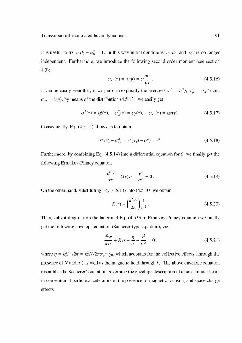
Transverse self-modulated beam dynamics 91
It is useful to fix γ0 β0 − α20 = 1. In this way initial conditions γ0, β0, and α0 are no longer
independent. Furthermore, we introduce the following second order moment (see section
4.3):
σrp(τ) = 〈rp〉 = σdσdτ
. (4.5.16)
It can be easily seen that, if we perform explicitly the averages σ2 = 〈r2〉, σ2p⊥ = 〈p2〉 and
σrp = 〈rp〉, by means of the distribution (4.5.13), we easily get
σ2(τ) = εβ(τ), σ2p(τ) = εγ(τ), σrp(τ) = εα(τ) . (4.5.17)
Consequently, Eq. (4.5.15) allows us to obtain
σ2 σ2p − σ
2rp = ε2(γ β − α2) = ε2 . (4.5.18)
Furthermore, by combining Eq. (4.5.14) into a differential equation for β, we finally get the
following Ermakov-Pinney equation
d2σ
dτ2 + k(τ)σ −ε2
σ3 = 0 . (4.5.19)
On the other hand, substituting Eq. (4.5.13) into (4.5.10) we obtain
K(τ) =
(k2
sλ0
2π
)1σ2 . (4.5.20)
Then, substituting in turn the latter and Eq. (4.5.9) in Ermakov-Pinney equation we finally
get the following envelope equation (Sacherer-type equation), viz.,
d2σ
dτ2 + K σ +η
σ−ε2
σ3 = 0 , (4.5.21)
where η = k2sλ0/2π = k2
s N/2πσzn0γ0, which accounts for the collective effects (through the
presence of N and n0) as well as the magnetic field through ks. The above envelope equation
resembles the Sacherer’s equation governing the envelope description of a non-laminar beam
in conventional particle accelerators in the presence of magnetic focusing and space charge
effects.

Transverse self-modulated beam dynamics 92
4.5.2 Self-modulation analysis by means of the Sagdeev potential
In order to perform an analysis of the self-modulation due to the PWF interaction in the
strongly nonlocal regime and aberration-less approximation, we use the method of Sagdeev
potential (or pseudo-potential) that can be constructed from the envelope Eq. (4.5.21). To
this end, we introduce the following dimensionless quantities:
τ = ksτ , σ = ksσ , K = K/k2s , ε = ksε .
Then, Eq. (4.5.21) can be cast as the motion equation of a single particle of unitary mass
d2σ
dτ2 = −∂Vs(σ)∂σ
, (4.5.22)
where
Vs(σ) =12
Kσ2 +12η ln σ2 +
ε2
2σ2 . (4.5.23)
Note that the initial conditions of Eq. (4.5.21) are:
σ0 ≡ σ(τ = 0) and σ′
0 ≡ (dσ/dτ)τ=0 .
Once these conditions are fixed, the mechanical energy (which is constant) of a representative
point in the σ - space is fixed, i.e.,
E =12
(dσdτ
)2
+12
Kσ2 +12η ln σ2 +
ε2
2σ2 =12σ′
20 +
12
Kσ20 +
12η ln σ2
0 +ε2
2σ20
.
Then, we can analyse the features of the corresponding motion that characterizes the evolu-
tion of σ(τ). This evolution includes in particular the features related to the stability/instability.
Figures 4.7 and 4.8 display the Sagdeev potential Vs(σ), i.e., Eq. (4.5.23) and the corre-
sponding numerical solution of the Eq. (4.5.22) [namely, solution of Eq. (4.5.21)] for given
initial conditions (σ0 = 1.5, σ′0 = 0) and different parameters K and η. From all the dis-
played cases, it is clear that the self-modulation is stable. This is not only a result for the
given initial conditions and the choices of the parameters. In fact, the analysis of Eq. (4.5.23)
for arbitrary values of K and η leads to conclude that the potential well is always trapping.

Transverse self-modulated beam dynamics 93
Figure 4.7: Sagdeev potential Vs (left) as defined by Eq. (4.5.23) and the correspondingnumerical solution (right) of the Eq. (4.5.21) in absence of external magnetic field, wherethe plot of Vs is scaled by a factor 105.
Figure 4.8: Sagdeev potential Vs (left) as defined by Eq. (4.5.23) and the correspondingnumerical solution (right) of the Eq. (4.5.21) in the presence of a strong external magneticfield, where the plot of Vs is scaled by a factor 105.
If the energy E coincides with the minimum of the potential well (σ0 = σ), the beam is in a
stationary state (self-equilibrium) and its spot size does not change, being fixed to the initial
value σ0 (note that σ′0 = 0), according to Eq. (4.5.21), i.e.,
K σ +η
σ−ε2
σ3 = 0 , (4.5.24)
where we have expressed Eq. (4.5.21) in terms of the dimensionless quantities and imposed
the equilibrium condition d2σ/dτ2 = 0. Note that in Figures 4.7 - 4.9, we have fixed the
parameters in such a way that σ ∼ 0.025. This facilitates the analysis we are going to
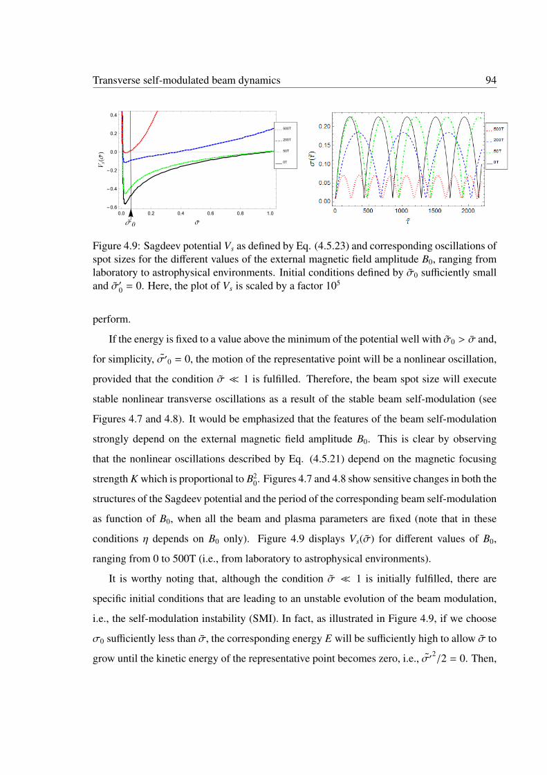
Transverse self-modulated beam dynamics 94
0.0 0.2 0.4 0.6 0.8 1.0-0.6
-0.4
-0.2
0.0
0.2
0.4
σ
Vs(σ)
0T
50T
200T
500T
σ0
Figure 4.9: Sagdeev potential Vs as defined by Eq. (4.5.23) and corresponding oscillations ofspot sizes for the different values of the external magnetic field amplitude B0, ranging fromlaboratory to astrophysical environments. Initial conditions defined by σ0 sufficiently smalland σ′0 = 0. Here, the plot of Vs is scaled by a factor 105
perform.
If the energy is fixed to a value above the minimum of the potential well with σ0 > σ and,
for simplicity, σ′0 = 0, the motion of the representative point will be a nonlinear oscillation,
provided that the condition σ 1 is fulfilled. Therefore, the beam spot size will execute
stable nonlinear transverse oscillations as a result of the stable beam self-modulation (see
Figures 4.7 and 4.8). It would be emphasized that the features of the beam self-modulation
strongly depend on the external magnetic field amplitude B0. This is clear by observing
that the nonlinear oscillations described by Eq. (4.5.21) depend on the magnetic focusing
strength K which is proportional to B20. Figures 4.7 and 4.8 show sensitive changes in both the
structures of the Sagdeev potential and the period of the corresponding beam self-modulation
as function of B0, when all the beam and plasma parameters are fixed (note that in these
conditions η depends on B0 only). Figure 4.9 displays Vs(σ) for different values of B0,
ranging from 0 to 500T (i.e., from laboratory to astrophysical environments).
It is worthy noting that, although the condition σ 1 is initially fulfilled, there are
specific initial conditions that are leading to an unstable evolution of the beam modulation,
i.e., the self-modulation instability (SMI). In fact, as illustrated in Figure 4.9, if we choose
σ0 sufficiently less than σ, the corresponding energy E will be sufficiently high to allow σ to
grow until the kinetic energy of the representative point becomes zero, i.e., σ′2/2 = 0. Then,

Transverse self-modulated beam dynamics 95
if the magnetic field is strong enough, its trapping effect limits the excursion of σ oscillations
to values that are still of the same order of magnitude of σ0 (Figure 4.9). However, if B0
is zero or assumes relatively small values, σ can easily grow until one or two orders of
magnitude greater than σ0. This aspect is deepen in Section 4.6 from qualitative point of
view, and in Section 4.7 from quantitative point of view.
4.6 Qualitative stability analysis
The analysis of the displayed plots leads to conclude that, during the beam evolution, pro-
vided that ideally the system is always in the strongly nonlocal regime, the self-modulation
is stable and the potential well is always trapping. However, as we have already indicated
above, this condition is fulfilled provided that∣∣∣∇2⊥Uw
∣∣∣ k2s |Uw| (i.e., σ 1). Therefore,
for a suitable choice of the initial conditions, such that σ satisfies this inequality, Figure
4.9 shows that the envelope self-modulation is stable and represents periodic solutions in
σ. This corresponds to fix the total energy E to relatively small values, in Figure 4.9 for
some of the profiles of the Sagdeev potential. If the energy E coincides with the minimum
of the potential well (i.e., σ0 = σ), the beam is in a stationary state (self-equilibrium) and
its spot size does not change, being fixed to the initial value σ0 (note that (dσ/dτ)τ=0 = 0),
according to Eq. (4.5.22). If the energy is fixed to a value above the minimum of the poten-
tial well with σ0 > σ, the motion of the representative point will be a nonlinear oscillation,
provided that the condition σ 1 is still fulfilled. In particular, values of E that are very
close to the minimum imply harmonic oscillations of σ. However, as B0 increases, sensitive
changes in both the structure of the Sagdeev potential and the period of the corresponding
beam self-modulation are observed in such a way that the beam spot size will execute more
and more stable nonlinear transverse oscillations. It is worthy noting that, although the con-
dition σ 1 is initially fulfilled, there are specific initial conditions that lead to an unstable
evolution of the beam modulation, i.e., SMI. In fact, as illustrated in Figure 4.9, if we choose
σ0 sufficiently less than σ, the corresponding energy E will be sufficiently high to allow σ to

Transverse self-modulated beam dynamics 96
Figure 4.10: Qualitative plot of Vs over all the three different regimes.
grow until the kinetic energy of the representative point becomes zero, i.e., 1/2 (dσ/dτ)2 = 0.
Then, if the magnetic field is strong enough, its trapping effect limits the excursion of σ os-
cillations to values that are still of the same order of magnitude of σ0. However, if B0 = 0
Figure 4.11: Qualitative plot of Vs over all the regimes with a qualitative smoothing of themoderately non-local regime.
or assumes relatively small values, σ can easily grow and becomes much greater than σ0.
Otherwise, when this is just about to happen, the condition σ << 1 is no longer fulfilled
and, therefore, the system enters progressively into the moderately nonlocal regime (i.e.,
σ ∼ 1) and then into the purely local regime (i.e., σ >> 1) [58]. We conclude that, although
Transverse self-modulated beam dynamics 97
the system starts with an initial condition falling into the strongly nonlocal regime, it may
rapidly violate the condition σ << 1 in such a way that its time evolution leads finally the
beam to the region of local regime where the self modulation becomes unstable. To study
this physical circumstance, we restrict our analysis to the case of B0 = 0 (ks = kp). It is
now useful to plot it as function of the dimensionless variable σ ≡ kpσ. According to Figure
4.10, the plot can be qualitatively divided into the three regions of σ, ranging from σ = 0 to
at least σ ∼ 10−102, corresponding to strongly nonlocal (i.e., σ 1), moderately non local
(i.e., σ ∼ 1) and purely local (i.e., σ 1) regimes, respectively. Therefore, the Sagdeev
potential should assume different shapes in the different regions. This implies that, out of
the region σ 1, the Sagdeev potential has to be determined starting with the appropriate
Vlasov-Poisson-type system of equations. Since we are interested in providing a qualitative
explanation of the unstable evolution of the self-modulation, we determine the analytical
expression of the Sagdeev potential in the purely local region. Then, we try to approach
qualitatively the moderately nonlocal region just by prolonging, one toward another, the plot
of the strongly nonlocal region and the plot of the purely local region, respectively. The in-
tersection of these two branches is illustrated in Figure 4.10, where the point of intersection
is denoted by P∗. In the σ-space it corresponds to the value σ∗. On the scale of the potential
adopted in Figure 4.10, the branch of the purely local region, compared to the nonlocal one,
appears practically constant, because it varies much slowly in σ. According to the analytical
treatment presented before, these two branches are respectively given by:
Vs1(σ) =12η ln σ2 +
ε2
2σ2 , 0 < σ ≤ σ∗ , (4.6.1)
Vs2(σ) =12
(ε2
σ20
−12
nb
n0γ0
)σ2
0
σ2 + C0 , σ ≥ σ∗ , (4.6.2)
where σ0 = σ(0), and
C0 =12η ln σ∗2 +
14
nb
n0γ0
σ20
σ∗2
is the constant which allows the continuity between the two branches. Figure 4.11 displays
qualitatively these two brunches once a qualitative smoothing of the moderately non-local
Transverse self-modulated beam dynamics 98
regime is done. This, of course, is only a qualitative way to connect the nonlocal region
with the local one. From Figures 4.10 and 4.11 it is evident that, with initial conditions σ0
falling in the strongly nonlocal region (i.e., σ0 1) and such that the total energy of the
representative point in the Sagdeev potential is ≤ E, the variation in σ are stable (periodic
self-modulations). But if the initial conditions correspond to a total energy which is > E,
then the representative point is no longer trapped in the potential. This corresponds to a
progressive increasing of σ, i.e., to an unstable evolution of the beam envelope modulations.
It is worthy noting that the flatness of the asymptotic region of σ (i.e., purely local
regime) does not depend on the sign of the difference(ε2
σ20− 1
2nb
n0γ0
). However, it is easy
to see that the time evolution in the purely local region is given by
σ2(τ) =
(ε2
σ20
−12
nb
n0γ0
)(τ − τ∗)2
+ σ∗2 , (4.6.3)
where τ = kpτ and τ∗ is the timelike value of τ such that σ(τ∗) = σ∗. Therefore, the growth
of σ is compatible only with the positive value of the difference(ε2
σ20− 1
2nb
n0γ0
).
4.7 Quantitative analysis of beam self-modulation in thearbitrary regime
4.7.1 General solution of Uw
In this section we provide a quantitative description of the self-modulated dynamics of a
cylindrically symmetric beam beyond the diverse special regimes that have been considered
in the previous section, such as the nonlocal (strong and moderate) and purely local cases.
Here, we develop a more general approach finalised to carry out self-consistent envelope
description associated with the Vlasov-Poisson-type system keeping both terms of the left-
hand side of Eq. (4.2.2), i.e., ∇2⊥Uw and k2
sUw. To this end, we assume that the system is not
far from the local thermal equilibrium. In this way, the solution of the Vlasov equation, i.e.,
∂ f∂τ
+ p∂ f∂r−∂V∂r
∂ f∂p
= 0 , (4.7.1)

Transverse self-modulated beam dynamics 99
where f = f (r, p, τ) is the cylindrically symmetric distribution function and
V = V(r, τ) =12
Kr2 + Uw(r, τ) ,
can be approximated by the following form:
f (r, p, τ) = nb(r, σ(τ))e−p2/σ2
p
πσ2p, (4.7.2)
where σ2p(τ) = 〈p2〉 and σ2(τ) = 〈r2〉. By introducing the dimensionless quantities: r = ksr,
τ = ksτ, p = ks p, σ = ksσ, and σp = ksσp, solution (4.7.2) can be cast as
f (r, p, τ) = nb(r, σ(τ) )e− p2/σ2
p
πσ2p, (4.7.3)
and the Poisson-type equation (4.2.2) in cylindrical co-ordinates, i.e.,
1r∂
∂r
(r∂Uw
∂r
)− k2
sUw = k2sλ nb , (4.7.4)
can be cast as∂2Uw
∂r2 +1r∂Uw
∂r− Uw = λ nb , (4.7.5)
where, Uw = Uw(r, σ) and λ = 1/n0γ0.
Note that we have explicitly indicated the dependence of f on τ also trhough the time depen-
dence of σ(τ) and σp(τ), respectively. Once the time evolution of σ is known, the time
dependence of nb is known, as well. Therefore, starting from an initial condition, i.e.,
σ0 = σ(τ = 0) and σ′0 = σ′(τ = 0), our analysis will allow us to study the envelope
evolution of the beam not far from the local thermal equilibrium. However, such an evolu-
tion can be stable and unstable, being dependent on the initial conditions. Therefore, we are
looking for suitable criteria that allows us to predict the stable or unstable evolution of the
beam envelope, just on the basis of the given initial conditions. To this end, we need to find
the envelope equation corresponding to our physical problem.
Equation (4.7.5) has the following solution
Uw(r, σ) = −λ
[K0(r)
∫ r
0I0(r1)nb(r1, σ)r1dr1 + I0(r)
∫ ∞
rK0(r2)nb(r2, σ)r2dr2
](4.7.6)
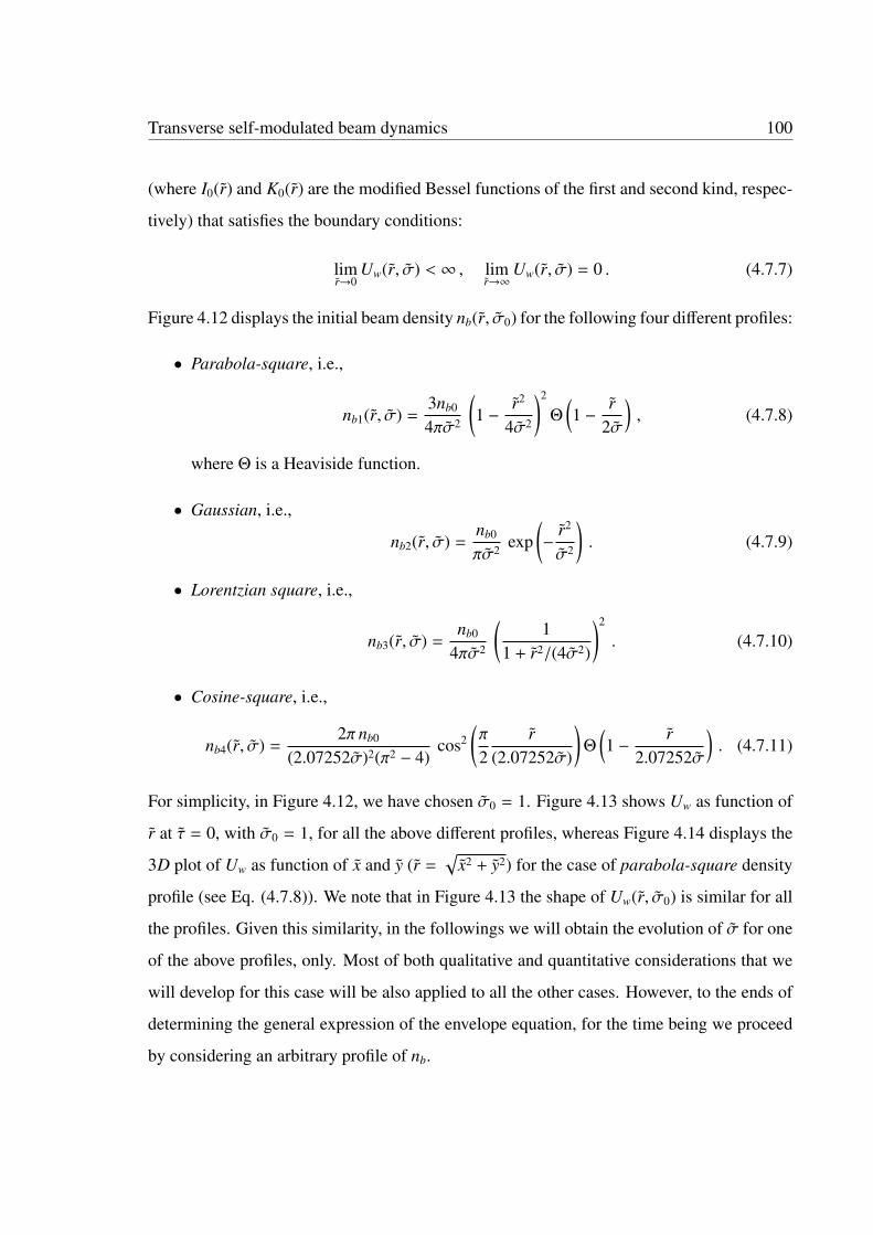
Transverse self-modulated beam dynamics 100
(where I0(r) and K0(r) are the modified Bessel functions of the first and second kind, respec-
tively) that satisfies the boundary conditions:
limr→0
Uw(r, σ) < ∞ , limr→∞
Uw(r, σ) = 0 . (4.7.7)
Figure 4.12 displays the initial beam density nb(r, σ0) for the following four different profiles:
• Parabola-square, i.e.,
nb1(r, σ) =3nb0
4πσ2
(1 −
r2
4σ2
)2
Θ
(1 −
r2σ
), (4.7.8)
where Θ is a Heaviside function.
• Gaussian, i.e.,
nb2(r, σ) =nb0
πσ2 exp(−
r2
σ2
). (4.7.9)
• Lorentzian square, i.e.,
nb3(r, σ) =nb0
4πσ2
(1
1 + r2/(4σ2)
)2
. (4.7.10)
• Cosine-square, i.e.,
nb4(r, σ) =2π nb0
(2.07252σ)2(π2 − 4)cos2
(π
2r
(2.07252σ)
)Θ
(1 −
r2.07252σ
). (4.7.11)
For simplicity, in Figure 4.12, we have chosen σ0 = 1. Figure 4.13 shows Uw as function of
r at τ = 0, with σ0 = 1, for all the above different profiles, whereas Figure 4.14 displays the
3D plot of Uw as function of x and y (r =√
x2 + y2) for the case of parabola-square density
profile (see Eq. (4.7.8)). We note that in Figure 4.13 the shape of Uw(r, σ0) is similar for all
the profiles. Given this similarity, in the followings we will obtain the evolution of σ for one
of the above profiles, only. Most of both qualitative and quantitative considerations that we
will develop for this case will be also applied to all the other cases. However, to the ends of
determining the general expression of the envelope equation, for the time being we proceed
by considering an arbitrary profile of nb.
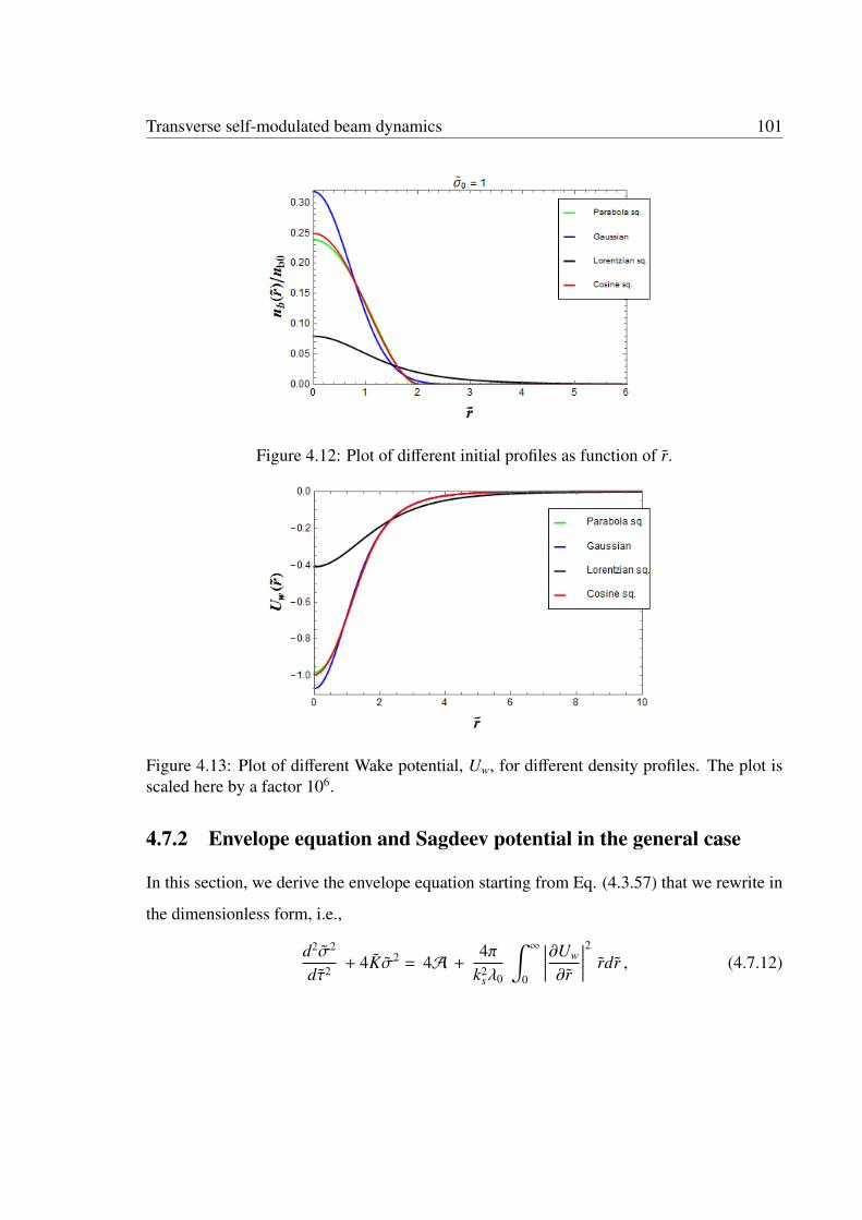
Transverse self-modulated beam dynamics 101
Figure 4.12: Plot of different initial profiles as function of r.
Figure 4.13: Plot of different Wake potential, Uw, for different density profiles. The plot isscaled here by a factor 106.
4.7.2 Envelope equation and Sagdeev potential in the general case
In this section, we derive the envelope equation starting from Eq. (4.3.57) that we rewrite in
the dimensionless form, i.e.,
d2σ2
dτ2 + 4Kσ2 = 4A +4π
k2sλ0
∫ ∞
0
∣∣∣∣∣∂Uw
∂r
∣∣∣∣∣2 rdr , (4.7.12)

Transverse self-modulated beam dynamics 102
Figure 4.14: 3D plot of plasma wake potential, Uw(r) for the parabola-square profile wherer =
√x2 + y2. The plot is scaled here by a factor 106.
where K = K/k2s . We multiply the latter by dσ2/dτ. Then, we integrate one time with respcet
to τ, obtaining:
2(dσdτ
)2
+ 2Kσ2 = 4A +2σ2
∫G( ˜σ) σ dσ +
E0
σ2 , (4.7.13)
where
G(σ) =4π
k2sλ0
∫ ∞
0
∣∣∣∣∣∂Uw(r, σ)∂r
∣∣∣∣∣2 rdr , (4.7.14)
and E0 is an integration constant, which can be evaluated by using the initial conditions, i.e.,
E0 = 2σ20σ′20 + 2Kσ4
0 − 4Aσ20 − 2
[∫G(σ) σ dσ
]σ=σ0
. (4.7.15)
Now, we expand d2σ2/dσ2 in Eq. (4.7.12), i.e., d2σ2/dσ2 = 2 (dσ/dτ)2 + 2σd2σ/dτ2, then
combine this with Eq. (4.7.13). We finally obtain the following envelope equation:
d2σ
dτ2 + Kσ +E0
2σ3 +1σ3
∫G(σ) σ dσ −
G(σ)2σ
= 0 . (4.7.16)
In a way fully similar to the one shown in the previous sections, we introduce also here the
definition of Sagdeev potential, i.e.,
d2σ
dτ2 = −∂Vs
∂σ.

Transverse self-modulated beam dynamics 103
Then, unless an arbitrary constant, we get:
Vs(σ) =12
Kσ2 −E0
4σ2 −1
2σ2
∫σ
G(σ′) σ′ dσ′ . (4.7.17)
Note that in Eqs. (4.7.15) - (4.7.17) the integration in dσ is indefinite. Furthermore, the last
two terms at left-hand side of Eq. (4.7.16) and at right-hand side of Eq. (4.7.17) have to be
evaluated explicitly by substituting the explicit form of nb(r, σ) in Eq. (4.7.6), as we do in
the next section.
Figure 4.15: Vs as function of σ for the entire range of values and for a relatively small pointof minimum, i.e., σ = 0.2.
4.7.3 Analysis of the envelope self-modulation in the general case
Once we have replaced the explicit form of the beam density in Eq. (4.7.6), we have eval-
uated numercally Uw(r, σ). The latter, in turn has been used to evaluate numerically the
function G(σ), as defined by Eq. (4.7.14). Therefore, the numerical knowledge of G(σ)
has allowed us to determine numerically the Sagdeev potential defined by Eq. (4.7.17) and
to integrate numerically the envelope equation (4.7.16) for given initial conditions. As we
already pointed out in the previous sections, we have performed this analysis by considering
only the beam profile defined by Eq. (4.7.8), since the features of the other profiles (Eqs.

Transverse self-modulated beam dynamics 104
Figure 4.16: Vs as function of σ ranging in the nonlocal region, for a very small point ofminimum, i.e., σ = 0.09.
E = -0.19
0.0 0.5 1.0 1.5 2.0-0.25
-0.20
-0.15
-0.10
-0.05
0.00
0.05
0.10
σ˜
Vs(σ˜
)
σ˜0 = 0.15, (dσ
˜/dτ˜)
τ∼=0
= 0, B0 = 0, σ = 0.09
0 2 4 6 8 10 12 14
0.06
0.08
0.10
0.12
0.14
τ˜
σ˜(τ˜)
σ˜0 = 0.15, (dσ
˜/dτ˜)
τ∼=0
= 0, B0 = 0, σ = 0.09
Figure 4.17: Left: Vs as function of σ, for a very small point of minimum, i.e., σ = 0.09.Right: envelope oscillations corresponding to initial conditions that fix E < 0 (see left) abovethe minimum, but below the plateau, i.e., E = −0.19.
(4.7.9) - (4.7.11)) are very similar. Due to this similarity, the analysis permits us extrapolate
considerations and write that are the same for all cylindrically symmetric bell-like shaped
density profiles. We restrict our discussion to the case of B0 = 0.
Figures 4.15 and 4.16 display the structure of Vs(σ) in two different scales of σ. Figure
4.15 shows almost entire shape of Vs(σ), whereas Figure 4.16 shows s similar structure on
a smaller scale of σ. In all profiles obtained (including a number is not displayed here),
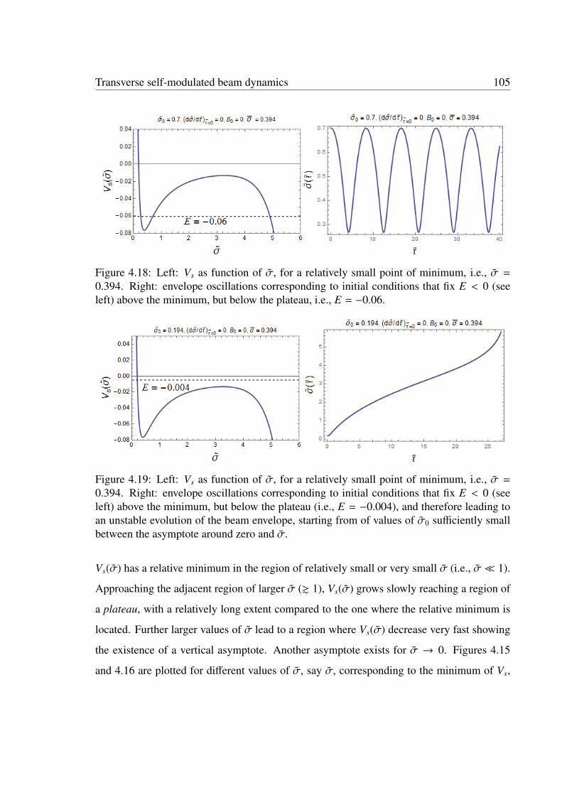
Transverse self-modulated beam dynamics 105
Figure 4.18: Left: Vs as function of σ, for a relatively small point of minimum, i.e., σ =
0.394. Right: envelope oscillations corresponding to initial conditions that fix E < 0 (seeleft) above the minimum, but below the plateau, i.e., E = −0.06.
Figure 4.19: Left: Vs as function of σ, for a relatively small point of minimum, i.e., σ =
0.394. Right: envelope oscillations corresponding to initial conditions that fix E < 0 (seeleft) above the minimum, but below the plateau (i.e., E = −0.004), and therefore leading toan unstable evolution of the beam envelope, starting from of values of σ0 sufficiently smallbetween the asymptote around zero and σ.
Vs(σ) has a relative minimum in the region of relatively small or very small σ (i.e., σ 1).
Approaching the adjacent region of larger σ (& 1), Vs(σ) grows slowly reaching a region of
a plateau, with a relatively long extent compared to the one where the relative minimum is
located. Further larger values of σ lead to a region where Vs(σ) decrease very fast showing
the existence of a vertical asymptote. Another asymptote exists for σ → 0. Figures 4.15
and 4.16 are plotted for different values of σ, say σ, corresponding to the minimum of Vs,
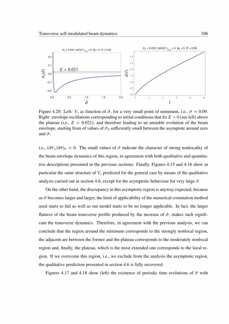
Transverse self-modulated beam dynamics 106
E = 0.021
0.0 0.5 1.0 1.5 2.0
-0.2
-0.1
0.0
0.1
0.2
σ˜
Vs(σ˜
)
σ˜0 = 0.033, (dσ
˜/dτ˜)
τ∼=0
= 0, B0 = 0, σ = 0.09
0 2 4 6 8 100.0
0.5
1.0
1.5
2.0
2.5
3.0
τ˜
σ˜(τ˜)
σ˜0 = 0.033, (dσ
˜/dτ˜)
τ∼=0
= 0, B0 = 0, σ = 0.09
Figure 4.20: Left: Vs as function of σ, for a very small point of minimum, i.e., σ = 0.09.Right: envelope oscillations corresponding to initial conditions that fix E > 0 (see left) abovethe plateau (i.e., E = 0.021), and therefore leading to an unstable evolution of the beamenvelope, starting from of values of σ0 sufficiently small between the asymptote around zeroand σ.
i.e., (∂Vs/∂σ)σ = 0. The small values of σ indicate the character of strong nonlocality of
the beam envelope dynamics of this region, in agreement with both qualitative and quantita-
tive descriptions presented in the previous sections. Finally, Figures 4.15 and 4.16 show in
particular the same structure of Vs predicted for the general case by means of the qualitative
analysis carried out in section 4.6, except for the asymptotic behaviour for very large σ.
On the other hand, the discrepancy in this asymptotic region is anyway expected, because
as σ becomes larger and larger, the limit of applicability of the numerical comutation method
used starts to fail as well as our model starts to be no longer applicable. In fact, the larger
flatness of the beam transverse profile produced by the increase of σ, makes such signifi-
cant the transverse dynamics. Therefore, in agreement with the previous analysis, we can
conclude that the region around the minimum corresponds to the strongly nonlocal region,
the adjacent are between the former and the plateau corresponds to the moderately nonlocal
region and, finally, the plateau, which is the most extended one corresponds to the local re-
gion. If we overcome this region, i.e., we exclude from the analysis the asymptotic region,
the qualitative prediction presented in section 4.6 is fully recovered.
Figures 4.17 and 4.18 show (left) the existence of periodic time evolutions of σ with

Transverse self-modulated beam dynamics 107
different values of the initial conditions and σ, respectively. This, in fact, corresponds to the
values of the conserved quantity
E =12σ′
20 + Vs(σ0) (4.7.18)
that are below the plateau (and therefore, E < 0), where for simplicity σ′0 = 0 for all cases.
The plots on the right, confirm such a prediction.
Figures 4.19 and 4.20 display a different behaviour. Plots on the left regards value of
σ0 and σ corresponding two values of E (negative of positive) that are above the plateau.
From there, it is evident that we predict motion that are not periodic with unstable evolution.
This is confirmed by the plots on he right. In particular, such unstable evolution correspond
to initial conditions belonging to the strongly nonlocal region between the asymptote and
the minimum of Vs. This is the clear evidence of the envelope self-modulation instability
occurrence.
4.8 Conclusions
We have carried out an analysis of the transverse self-modulation experienced by a cylin-
drically symmetric ultra-relativistic and nonlaminar driving beam while interacting with the
surrounding plasma. This has been accomplished by using the pair of 3D Vlasov-Poisson
equations found in Chapter 3, that here has been specialized to the purely 2D transverse case
in cylindrical symmetry. The plasma has been supposed to be overdense, cold, and magne-
tized. Due to the conditions of very long beam, the self-consistent PWF mechanism works
very efficiently to sensitively characterize the self-modulated dynamics.
We have implemented the Vlasov-Poisson-type system of equation with the virial equations.
Their coupling have provided a suitable description of the beam envelope self-modulation.
Remarkably, we have shown the importance of the constants of motion involved in such a
description, that have allowed us to obtain suitable beam envelope equations, i.e., ordinary
differential equations for the beam spot size that are easily integrated analytically and/or
numerically. To approach also our problem qualitatively, we have used the method of the

Transverse self-modulated beam dynamics 108
pseudo potential (or Sagdeev potential) that is associated with these envelope equations.
We have first carried out an analysis in two different limiting cases, i.e., the local case (the
beam spot size is much greater than the plasma wavelength) and the strongly nonlocal case
(the beam spot size is much smaller than the plasma wavelength) where several types of
self-modulation, in terms of focusing, defocusing and betatron-like oscillations, have been
obtained and the criteria for instability, such as collapse and self-modulation instability, have
been formulated. To this ends, within the context of the envelope description, we have found
suitable envelope equations, i.e., ordinary differential equations for the beam spot size, that
have been easily integrated analytically and physically described in terms of the Sagdeev
potential method.
Then, the analysis has been extended to the general case where the beam spot size and the
plasma wavelength are not necessarily constrained as in the local or strongly nonlocal cases.
In these conditions, we have performed a semi-analytical and numerical analysis by means of
the virial equations, where the above methods of the envelope equations and Sagdeev poten-
tial have been used, as well. To this end, criteria for predicting stability and self-modulation
instability have been suitably provided.

Chapter 5
Longitudinal instability analysis ofbeam-plasma system
We carry out an analysis of the beam modes that are originated by perturbing the ‘beam-plasma’
system in the purely longitudinal case. This is done by considering the pair of 3D Vlasov-Poisson-
type equation, presented in Chapter 3 that are specialized to the case in which the transverse driving
beam dynamics is disregarded and only the longitudinal dynamics becomes effective. To this end, we
perturb the Vlasov-Poisson-type system up to the first order, then take the Fourier transform to reduce
the Vlasov-Poisson system to a set of algebraic equations in the frequency and wavenumber domain,
from which we easily get a Landau-type dispersion relation for the beam modes, that is fully similar
to the one holding for plasma modes. First, we consider the case of a monochromatic beam (i.e., cold
beam, that is described by a distribution function in the form of delta-function in p space) for which
the existence of a purely growing mode is shown and a simple stability criterion formulated. Then,
by taking into account a unperturbed distribution function with finite, relatively small width (small
thermal correction), the Landau approach, widely used in other physics area, leads to obtain both
the dispersion relation for the real part (showing all the possible beam modes in the diverse regions
of the wavenumber) and an expression for the imaginary part of the frequency (showing the stable or
unstable character of the beam modes), which suggests a simple stability criterion.
109

Instability analysis 110
5.1 Introduction
As we have shown in the previous chapters, the interaction of a relativistic beam with the
plasma involves self-consistent collective and nonlinear mechanisms that lead to the beam
self-modulation. In particular, in Chapter 4, we have presented the envelope self-modulation
that has shown the occurrence of several self-consistent transverse electromechanical effects
and investigated the conditions for the occurrence of the self-modulation instability. Analo-
gous effects occur also in the longitudinal dynamics. In particular, a high-intensity electron
beam of finite extent can be subjected to longitudinal instabilities. The nonlinear collective
effects that take place in the longitudinal dynamics of charged-particle beams while trav-
elling in a plasma constitute a large-body of phenomena in the plasma-based accelerators.
The standard theory of collective longitudinal relativistic beam dynamics in accelerators is
based on kinetic theory described by the Vlasov equation, which in general is coupled with
a Poisson-type equation describing the plasma wake field excitations.
In this chapter, we carry out an instability analysis within the linearized kinetic the-
ory of the self-consistent beam-plasma interaction, where the Landau damping plays a role.
This is done by assuming that the beam-plasma system is governed by the self-consistent
Vlasov-Poisson-type pair of equation. We take into account a cold, unmagnetized plasma,
constituted by immobile ions (forming a backgroud of positive charge) and mobile electrons,
and a nonlaminar, relativistic charged particle beam travelling therein, along the longitudinal
direction (z). According to the concepts described in Chapter 2, in the purely longitudinal
case, the wake field and the wake potential reduce to the longitudinal electric field and the
scalar potential, respectively. Correspondingly, in absence of significant magnetic effects
(the vector potential can be fixed to zero), Eq. (2.1.14) reduces to:
F(ξ, τ) = q∂Ω(ξ, τ)∂ξ
. (5.1.1)
In case of free evolution, the plasma oscillations are governed by the differential equation
∂2Ω
∂ξ2 + k2p Ω = 0 , (5.1.2)

Instability analysis 111
whereas in the presence of the charged particle beam this equation contains, additionally, a
forcing term, i.e.,∂2Ω
∂ξ2 + k2p Ω = 4πqnb , (5.1.3)
where nb = nb(ξ, τ) is the volumic beam number density. It is related to the single-particle
distribution function f (ξ, p, τ) which is defined in the longitudinal 2D (ξ, p) phase space (p
being the longitudinal single-particle linear momentum conjugate of ξ). In fact, by denot-
ing with λ(ξ, τ) the longitudinal 1D number density (i.e., number of particles per unitary
longitudinal length), we have:
λ(ξ, τ) = nb(ξ, τ) πσ2⊥ ,
where σ⊥ is the effective beam transverse size (i.e., spot size). Thus, the following relation-
ship holds:
nb(ξ, τ) πσ2⊥ =
∫f (ξ, p, τ) dp . (5.1.4)
In addition, f (ξ, p, τ) obeys to the following purely longitudinal Vlasov equation (for details,
see Chapter 3):∂ f∂τ
+ p∂ f∂ξ
+q
mb0γ0c2
∂Ω
∂ξ
∂ f∂p
= 0 . (5.1.5)
We start from the equilibrium state that is described by the quantities:
np = n0 , nb = nb0 , Ω = Ω0 , and f = f0(p) ,
where np is the plasma electron density. Then, we perturb this state with small (i.e., first-
order) deviations, i.e.,
np(ξ, τ) = n0 + n1(ξ, τ) , nb(ξ, τ) = nb0 + nb1(ξ, τ) , Ω(ξ, τ) = Ω0 + Ω1(ξ, τ) ,
and
f (ξ, p, τ) = f0(p) + f1(ξ, p, τ) .
Here, n0, nb0, and Ω0 are constant quantities. Consequently, up to the first order, the system
of equations (5.1.3) - (5.1.5) reduces to:
k2p Ω0 = 4π q nb0 , (5.1.6)

Instability analysis 112
which defines the unperturbed wake potential in terms of the unperturbed beam density,
where
nb0 πσ2⊥ =
∫f0(p) dp , (5.1.7)
and
∂2Ω1
∂ξ2 + k2p Ω1 = 4πq nb1 , (5.1.8)
∂ f1
∂τ+ p
∂ f1
∂ξ+
qmb0γ0c2
∂Ω1
∂ξ
∂ f0
∂p= 0 , (5.1.9)
where
nb1 =1πσ2⊥
∫f1 dp . (5.1.10)
The linearized system of equations (5.1.8) - (5.1.10) governs the self-consistent spatiotem-
poral evolution of the PWF interaction in the case of purely longitudinal dynamics. Note the
full similarity between Eq. (5.1.8) and Eq. (2.7.5), which holds in the overdense regime (i.e.,
nb n0). Here, nb1 ( nb0 ∼ n0) plays the role that in Eq. (2.7.5) is played by nb as first
order quantity. This means that, in the case under discussion, the perturbation nb1 is actually
the source of the plasma wake field.
The linearization of the Vlasov-Poisson-type system of equations, offers the advantage, by
means of the Fourier transform, to reduce such system to a set of algebraic equations, lead-
ing to the dispersion relations, i.e., a relation between the frequency and the wave number of
each mode. This procedure is carried out in the next section.
5.2 Dispersion relation
The Fourier transformation transforms the system of equations (5.1.8) - (5.1.10) into the
following algebraic system of equations (∂/∂τ→ −iω/c and ∂/∂ξ → ik), i.e.,
(k2
p − k2)Ω1 = 4πq nb1 , (5.2.1)
i(pk −
ω
c
)f1 +
ikqΩ1
mb0γ0c2 f ′0 = 0 , (5.2.2)

Instability analysis 113
where f ′0 = d f0/dp and the quantities Ω1 = Ω1(k, ω), nb1 = nb1(k, ω) and f1 = f1(k, p, ω)
stand for the Fourier transforms of Ω1, nb1 and f1, respectively.
Then, by combining Eqs. (5.2.1) to (5.2.2), we easily get,
1 =ω2
b
γ0c2
1k2 − k2
p
∫ f ′0 dpp − ω
ck
. (5.2.3)
where ωb =(4πq2nb0/mb0
)1/2is the plasma frequency of the beam and
f0 = f0/(nb0πσ2⊥).
Therefore, Eq. (5.2.3) can be written as:
1 =η
k2 − 1
∫ f ′0 dp
p − ωk
, (5.2.4)
where η = (nb0/γ0n0) (q2/e2)(me0/mb0) is a positive constant, k2b = ω2
b/c2, and we have
introduces the following normalized quantities
ω = ω/ωp, k = k/kp.
We assume, for simplicity, that the beam under consideration is an electron beam, i.e., mb0 =
me0 and q = e. Hence the constant η becomes
η =1γ0
nb0
n0.
Once the profile of f0 is given, dispersion relation (5.2.4) can be suitably used to carry
out an analysis of the beam modes. Then, taking into account both the Landau damping
phenomenon and the instability occurrence, we try to formulate the instability criteria.
5.3 Monochromatic profile
We start to analyse the case when the beam is monochromatic (or cold), i.e., f0 ∝ δ(p). By
integrating by part the term at the right-hand side of Eq. (5.2.4) we obtain,
ω2 =η k2
k2 − 1. (5.3.1)

Instability analysis 114
Then, after writing ω = ωR + iωI , and assuming that k is real, we can divide the real from the
imaginary part. So that we finally find
ωR ωI = 0 , (5.3.2)
ω2R − ω
2I =
η k2
k2 − 1. (5.3.3)
• If ωI = 0, from Eq. (5.3.3) we get,
ωR = ±
√η |k|
√k2 − 1
. (5.3.4)
Then, since ωR is real, k2 > 1. In addition, since ωI = 0, the modes (k, ωR
(k))
described by dispersion relation (5.3.4) are stable.
• If ωR = 0, from Eq. (5.3.3) we get,
ωI = ±
√η |k|
√1 − k2
. (5.3.5)
Then, since ωI is real, k2 < 1.
According to Eq. (5.3.5), at fixed k, for any negative solution of ωI there is a positive solution
of ωI . This indicates instability of the corresponding beam mode which appears as a purely
growing mode.
Figure 5.1 and 5.2 show the plots of the dispersion relation i.e., ωR
(k)
and ωI
(k), for
an initial monochromatic beam profile and for a given ratio nb0/n0. The former displays the
stable modes that possess cut-off for both k and ωR. The latter, shows the purely growing
mode, whose growth rate, i.e., ωI , does not possess any cuf-off, but is limited in the range,
−1 < k < 1.
Note that for a plasma density n0 = 5 × 1017cm−3, the plasma frequency is ωp ' 4 × 10¹³
rad/s. Then, from the definition of ωR and ωI , we find that in Figures 5.1 and 5.2, |ωR| and
|ωI | range (from 0.4 to 2.4) ×1013 rad/s and (from 0 to 1.6) ×1013 rad/s, respectively.

Instability analysis 115
Figure 5.1: Variations of ωR with k for a monochromatic beam profile at fixed ratio nb0/n0.Here the solid lines indicate positive ωR and the dashed lines indicate negative ωR accordingto Eq. (5.3.4).
Figure 5.2: Variations of ωI with k for a monochromatic beam profile at fixed ratio nb0/n0.Here the solid lines indicate positive ωI and the dashed lines indicate negative ωI accordingto Eq. (5.3.5).
5.4 Non-monochromatic case: weak Landau damping andinstability
The beam is called non-monochromatic or warm when the distribution function f0(p) has a
finite width due to the presence of the random character of the particle motion. We assume
that f0(p) is a bell-like shaped function such that f0(−p) = f0(p), such as in the case of

Instability analysis 116
normalized parabola-square profile, i.e.,
f0(p) =1516
1√
7σp
(1 −
p2
7σ2p
)2
, −√
7σp ≤ p ≤√
7σp , (5.4.1)
and the case of normalized Gaussian profile, i.e.,
f0(p) =1√
2πσ2p
exp[−
p2
2σ2p
], −∞ < p < ∞ , (5.4.2)
where σp = 〈p2〉1/2. Furthermore, one can introduce reasonably the definition of temperature
T , i.e., σp ≡ vT ≡(kBT/mb0γ0c2
)1/2, where vT is the dimensionless thermal velocity.
We assume that vT is very small compared to the dimensionless phase velocity, i.e., ω/k,
of the beam perturbation: kvT/ω 1. Therefore, compared to the case of Eq. (5.3.4) of the
monochromatic beam (where ωI = 0), this condition represents a small deviation from the
delta function distribution. Then, the integral in Eq. (5.2.4) has to be solved according to the
Landau prescription [66, 67], i.e.,
1 =η
k2 − 1
∫PV
f ′0dp
p − ωk
+ iπ f ′0(ω
k
) , (5.4.3)
where∫
PVf ′0/(p − ω/k) dp stands for the Cauchy principal value and the second term in the
square bracket accounts for the residue. By performing the integration by parts in the integral
of Eq. (5.4.3), expanding the term (p − ω/k)−1 in powers of p, and taking into account the
assumptions of both symmetry and small deviation from the monochromatic case, one can
easily get, ∫PV
f ′0dp
p − ωk
=k2
ω2
(1 +
3k2v2T
ω2
), (5.4.4)
where, consistently with the above assumptions, we have truncated the expansion in p up
to the second power. The small deviation from the monochromatic case is therefore related
to the smallness of the quantity kvT/ω. For a given vT , it implies that f ′0(ωR/k
)is a small
quantity compared to the principal value. In turn, the smallness of the residue implies the
smallness of ωI , compared to ωR. Therefore, in Eqs. (5.4.3) and (5.4.4), we assume that
Instability analysis 117
ω = ωR + i ωI with the condition |ωI | |ωR|. Then, separating the real from the imaginary
parts, we obtain
ω2R =
η k2
k2 − 1
(1 +
3k2 v2T
ω2R
), k2 > 1 , (5.4.5)
which can be cast as,
ωR = ±
√η |k|
√k2 − 1
(1 +
3k2 v2T
ω2R
)1/2
, k2 > 1 . (5.4.6)
However, since kvT/ωR 1, in second term of right-hand side of the above mentioned
equation we can replace ωR by using Eq. (5.3.4). Therefore, Eq. (5.4.6) can be approximated
as:
ωR = ±
√η |k|
√k2 − 1
(1 +
32
v2T
η(k2 − 1)
), k2 > 1 , (5.4.7)
On the other hand, the imaginary part of the combination of Eqs. (5.4.3) and (5.4.4) gives
ωI =π
2η ωR
k2 − 1f ′0
(ωR
k
), k2 > 1 . (5.4.8)
Equation (5.4.8) shows that, for positive (negative) sign of the product ωR f ′0(ωRk
), ωI is posi-
tive (negative). If ωI is negative, the wave associated with the beam perturbation experiences
the damping effect. This is the phenomenon of Landau damping which is well known in plas-
mas [67] and in a number of other physics areas [68]. However, if ωI is positive the wave
amplitude grows and this circumstance indicates the instability of the beam perturbation.
As in the ordinary Landau damping occurring in plasmas, here we can provide the physi-
cal explanation in terms of wave-particle interaction. In fact, the beam is non-monochromatic,
i.e., its phase space distribution f0(p) is bell-like shaped [see the examples given by Eqs.
(5.4.1) and (5.4.2)]. Then for a given phase velocity of the beam density perturbation or
of the PWF perturbations (i.e., ω/ck), there are more particles with p < ω/ck (that are
taking energy from the wave) than the ones with p > ω/ck (that are giving energy to the
wave). Therefore, statistically, the wave experiences the phenomenon of damping (i.e., Lan-
dau damping). This effect, being in competition with the instability, contributes to the system

Instability analysis 118
stabilization. It is worthy noting that Landau damping disappears as the temperature of the
system goes to zero (cold beam or the monochromatic beam). The absence of such an effect
leads to instability that is, therefore, the analog of the two stream instability and represents a
purely growing mode.
Figure 5.3: Variation of ωR with k for bell-like shaped non-monochromatic beams for differ-ent beam temperatures at fixed energy and ratio nb0/n0 = 0.5.
Figure 5.4: Variation of ωR with k for bell-like shaped non-monochromatic beams for differ-ent beam temperatures at fixed energy and ratio nb0/n0 = 1.5.
In Figures 5.3 and 5.4, the solid lines indicate positive ωR and the dashed lines indicate
negative ωR, according to Eq. (5.4.7). These figures show ωR as function of k when the
distribution function is a bell-like shaped non-monochromatic, but exhibits a small width
due to the finite temperature. The different plots are given for different temperatures with
fixed γ0 and nb0/n0. Compared to the corresponding plot of the monochromatic case (Figure

Instability analysis 119
5.1), the case of T = 0 is recovered. As T increases, the horizontal asymptotes changes into
oblique axes, increasing gradually the cut-off frequency of each of the four sectors of the
plot. This produces a progressive enlargement of the gap between the domain of the positive
frequency and the one of the negative frequency, showing also a more “acute” shapes of each
plot. An important consequence of this deformation is the increasing of the absolute value
of both phase velocity and group velocity in all the permitted domains of k. In addition, the
deformation is stronger in the case of smaller energy of the beam (γ0).
5.5 Conclusions
We have carreid out an analysis of the beam modes that are originated by perturbing the
‘beam-plasma system’ in the purely longitudinal dynamics of a relativistic driving beam.
This has been accomplished by specializing to the 1D longitudinal case the pair of 3D
Vlasov-Poisson-type equation, presented in Chapter 3. To this end, we have perturbed the 1D
Vlasov-Poisson-type system up to the first order, then used the Fourier transform to reduce
the Vlasov-Poisson system to a set of algebraic equations in the frequency and wavenumber
domain. From the latter we have easily found the Landau-type dispersion relation for the
beam modes that is fully similar to the one holding for plasma modes. As a first case, we
have studied the dispersion relation in the case of monochromatic beam that is described by
a distribution function in the form of delta-function in p space). The analysis has shown the
existence of a purely growing mode and a simple stability criterion. Then, by taking into
account a non-monochromatic (i.e., a distribution function with a relatively small width due
to the finite temperature), the Landau approach has lead to obtain both the dispersion rela-
tion for the real part (showing all the possible beam modes in the diverse regions of the wave
number) and an expression for the imaginary part of the frequency, which has suggested a
simple stability criterion.

Chapter 6
The coupling impedance concept forPWF self-interaction
Starting from the collisionless Vlasov-Poisson-type system of equation for longitudinal beam dynam-
ics, that has been presented in Chapter 5, we formulate a novel approach in which we put forward the
concept of longitudinal coupling impedance associated with the beam-plasma interaction, in a way
fully similar to the one in use in conventional particle accelerator physics. As in the conventional
theory, the concept of coupling impedance seems to be very fruitful in a plasma-based accelerator
to schematize the self-interaction of the relativistic driving beam with the surrounding plasma. In
particular, it allows us to develop a simple instability analysis in the plane of the real and imaginary
parts of the impedance that is based on the Nyquist approach widely used in the control system theory.
Furthermore, we extend the Vlasov-Poisson-type system to the collision context with a simple model
of collisions between the plasma particles (actually plasma electrons) and the beam particles. Under
these assumptions, the role and the features of the coupling impedance defined here are compared to
the ones of the coupling impedance in conventional theory. Examples of specific physical situations
are finally illustrated.
6.1 Introduction
In a conventional particle accelerator, the coupling impedance schematizes the interaction of
a (relativistic) charged particle beam with the surrounding medium. This interaction involves
120

The coupling impedance concept for PWF 121
the wake fields that are produced by each charged particle of the beam [69]. Therefore, such
an interaction is a macroscopic (collective) manifestation of the beam in the surroundings.
A very effective way to describe such an interaction makes use of the concept of both im-
age charges and image currents [70, 71]. They are produced, for instance, on the metallic
walls of the vacuum chamber, by the charged particles of the beam. Therefore, they are the
sources of electric and magnetic fields which are moving behind the beam at the same its
speed (wake fields). However, there are some other sources of wake fields, such as the vari-
ations of the vacuum chamber geometric features, which produce scattered electromagnetic
fields. In general, one can distinguish short range wake fields influencing the single bunch
beam dynamics from the long range wake fields, influencing the multi-bunch beam dynam-
ics. However, restricting to the wake fields associated with the space charge effects, one can
see that sufficiently short bunches affect mainly the particle of another bunch moving behind.
However, as the beam becomes longer and longer, those fields affect more and more the par-
ticles of the beam itself. As we discuss later for plasma wake field (PWF) accelerators, in
analogy with the conventional accelerators, the dynamics of long enough single bunches is
sensitively affected by the wake fields. Then, the beam particles experience the effects of the
fields that they have themselves produced in the surroundings (self-interaction). Due to the
nature of the interaction between the beam and the surroundings, some reactive (capacitive
as well as inductive) energy related to the beam space charge and current is involved in the
system. In addition, the possible resistive character of the metallic walls experienced by the
image currents and the geometric variation of the pipe (leading to beam losses), involves
some resistive energy, as well. Therefore, in the domain of frequency and wave number, the
interaction of the beam with the surroundings can be effectively represented by a sequence of
elements of an electric transmission line. Each of these elements accounts for an equivalent
impedance per unitary length which is constituted by an equivalent capacitance, inductance
and resistance per unitary length. This is usually referred to as the coupling impedance, since
it schematizes the self-consistent interaction between the beam and the surrounding medium.
In 1959, Andrew M. Sessler, in collaboration with Carl Nielsen and Keith Symon, took

The coupling impedance concept for PWF 122
up the study of collective instabilities of a relativistic charged-particle beam that take place in
an accelerating machine, the so-called coherent beam instabilities (a special case of them is
the well known negative-mass instability) [72]. The approach of these researchers lead soon
to conclude that coherent instabilities are due to the beam space charge through the mecha-
nism of the self interaction that the same space charge experiences with the surroundings via
the image charges distributed on the wall of the vacuum chamber. It was the first exploration,
based on the Vlasov kinetic theory, that allowed them to realize the important role of the Lan-
dau damping [66] as a stabilizing effect acting to cure the coherent instabilities. The Landau
damping is, in fact, a phenomenon resulting from the interaction of space charge waves (the
so-called electrostatic waves arising in plasmas or in generic charged-particle systems, such
as beams) with the single particles. Namely, this is the interaction of a collective mode of
the system with a single individual (single-particle). In the single process of wave-particle
interaction, the energy can be transferred from the wave to the particle or from the particle to
the wave, provided that the phase velocity of the wave is slightly greater or slightly smaller
than the particle velocity, respectively. The resonance condition is established when these
velocities are the same. This means that wave and particles are actually interacting around
the resonance. Lev D. Landau demonstrated that, for single-humped thermal particle distri-
butions, the statistical energy balance coming from all the wave-particle interactions shows
that the space charge wave is damped and, therefore, it provides to contrast the wave growth
due to the instability. Then, the way in which the interplay between coherent instability and
Landau damping takes place works leading to stable or unstable evolution of the system.
The stability or the instability depends on precise conditions that are related to the coupling
impedance.
In subsequent studies with L. Jackson Laslett and V. Kelvin Neil [73] and Ernest Courant
[74], Sessler became interested in single bunches rather than a continuous beam, and he
realized that wall resistance is only one aspect of the general concept of impedance. The
latter was later developed in collaboration with Vittorio G. Vaccaro [75], who suggested to

The coupling impedance concept for PWF 123
formulate a more general definition of the coupling impedance that they applied to the col-
lective longitudinal dynamics of an azimuthally uniform beam. Although Sessler had a high
opinion of Vaccaro, this formulation was not soon accepted at CERN. Meanwhile, Vaccaro
was producing a subsequent work in collaboration with Alessandro G. Ruggiero [76], where
the previous approach to the longitudinal instability was improved and formalized in terms
of a stability criterion a la Nyquist, later sometimes referred to as Sessler-Ruggero-Vaccaro
criterion. After a few years, the concept of coupling impedance became more and more
popular in particle accelerator physics. Nowadays everyone uses their work to calculate,
measure, and control impedance in order to limit instabilities. [77].
6.2 Phenomenological platform of the beam-plasma inter-action
The interaction between charged-particle beams with plasmas touches a large variety of phe-
nomena, ranging from laboratory to space and astrophysical plasmas.
Part of these phenomena concern types of beam-plasma interactions in which the plasma
can be thought as a collection of streams. Each of them is constituted by different particle
species in terms of mass and charge. Such a system satisfies the global charge neutrality
condition. In linear theory, the multi-stream instability theory is the simplest approach to the
plasma instability that can be provided by both fluid and kinetic models. In particular, it is
very useful to approach the beam-plasma instability, such as Buneman instability [78, 79].
Note that here, the beam is not an object external to the plasma. It actually represents one
of its own components. Therefore, the self-consistent spatiotemporal evolution of the beam
takes place while contributing to satisfy the global neutrality conditions.
A different scenario appears when a charged-particle beam enters the plasma. In fact,
while the plasma components satisfy all together the global neutrality condition, the external
beam introduces an additional charge that cannot be balanced in the beam-plasma system.
The coupling impedance concept for PWF 124
The beam introduces a local charge density perturbation which the plasma tends to neutral-
ize locally. Contextually, a current density perturbation is introduced, as well. The resulting
electric and magnetic fields act locally on the particles of the system and, therefore, both
plasma and beam evolve in space and time self-consistently, according to the pair of Vlasov-
Poisson-type equations for the beam-plasma system. Then, the concept of the coupling
impedance in the beam-plasma interaction ruled by the PWF excitation can be introduced
after linearizing the Vlasov-Poisson-type system (around an unperturbed state) and taking
the Fourier transform of the resulting equations.
6.3 Vlasov-Poisson-type pair of equations
To perform an analysis of the linearized beam-plasma system dynamics by means of the
concept of coupling impedance, for simplicity, we confine our description to the case of
an electron beam. We take into account the case of a collisionless beam-plasma dynam-
ics, where a nonlaminar, relativistic, electron beam travelling through a cold, unmagnetized
plasma in the longitudinal direction. In general, this analysis can be easily applied to the
transverse case or extended to the 3D case. Then, the linearized pair of Vlasov-Poisson-type
equations governing the spatiotemporal longitudinal dynamics of our system (similar to the
system of equations given in Section 5.1) is(∂2
∂ξ2 + k2p
)Ω1 = k2
pme0ce2n0
Ib1
βπσ2⊥
, (6.3.1)
∂ f1
∂τ+ p
∂ f1
∂ξ+
(−e)me0γ0c2
∂Ω1
∂ξ
∂ f0
∂p= 0 , (6.3.2)
where Ω1 = Ω1 (ξ, τ), f0 = f0 (p) is the unperturbed distribution function, f1 = f1 (ξ, p, τ) is
the first-order correction of this distribution and
Ib1 (ξ, τ) = (−e)βc∫
f1 (ξ, p, τ) dp = −e)βcπσ2⊥nb1 (6.3.3)
is the perturbed beam-current. Here e and σ⊥ are the absolute value of the electron charge
and the transverse beam spot size, respectively.
The coupling impedance concept for PWF 125
Equation (6.3.1) is a linear equation relating nb1 (ξ, τ) to Ω1 (ξ, τ). Equation (6.3.2) ac-
counts for the slower evolution of the beam beyond the stationary state and it is coupled
with the former, therefore it is in principle a nonlinear equation. Then, the pair of equations
(6.3.1) - (6.3.2) governs the self-consistent spatio-temporal evolution of the PWF interaction.
6.4 Heuristic definition of coupling impedance
Here, we put forward the following heuristic definition of longitudinal coupling impedance
per unity length, say Z, which is fully similar to the heuristic definition given in conventional
accelerators [71]. Then, by denoting with Ω1 (k, ω) and Ib1 (k, ω) the Fourier transform of
Ω1 (ξ, τ) and Ib1 (ξ, τ), respectively, we define Z (k, ω) as
Z(k, ω) = −i kΩ1 (k, ω)Ib1 (k, ω)
. (6.4.1)
In principle, Z (k, ω) is a complex quantity. Then, in general, we can cast it as the sum of real
and imaginary part, i.e., Z (k, ω) = ZR (k, ω)+ i ZI (k, ω). By combining the Fourier transform
of both Eqs. (6.3.1) and (6.3.2), where (∂/∂τ→ −iω/c and ∂/∂ξ → ik), we get the following
dispersion relation of the beam-plasma system, viz.,
1 = −iηcZ (k, ω)
k
∫ f ′0(p)dpp − ω/ck
, (6.4.2)
where ηc = ω2b/(γ0c2) βcσ2
⊥/4, is a positive constant, f0 denotes the normalized equilibrium
distribution function and f′
0 (p) ≡ d f0/dp. This is the Landau-type dispersion relation. Each
possible mode (k, ω) of the system must satisfy it. For each mode (k, ω), if ZR , 0, the
coupling between beam and plasma involves some resistive energy that must be represented
by losses; whilst if ZI , 0, some reactive energy is involved in such a coupling, which means
that the energy is stored in the electric and magnetic parts of the PWFs.
6.5 Stability analysis
The spectrum of the possible modes is different for different explicit expression of Z (k, ω)
provided by Eq. (6.4.1) and the Fourier tranform of Eq. (6.3.1). For the specific case under
The coupling impedance concept for PWF 126
consideration here, the latter is:
(−k2 + k2p)Ω1 = k2
pme0ce2n0
Ib1
βπσ2⊥
. (6.5.1)
Then, by combining it with Eq. (6.4.1), we easily get the following conditions of compati-
bility
ZR = 0 ,Z(k)
k=
i ZI(k)k
⇒ZI(k)
k=
K0k2p
(k2 − k2p), (6.5.2)
where K0 = me0c/n0e2βπσ2⊥, and here we have assumed that k is a real quantity. These
conditions show that in the case under discussion the impedance is purely imaginary (i.e.,
purely reactive). In fact, we have assumed that the beam-plasma system is collisionless,
and this implies that there is no dissipation in the system. Consequently, dispersion relation
(6.4.2) becomes:
1 = ηcZI (k)
k
∫ f ′0(p)dpp − ω/ck
. (6.5.3)
6.5.1 Monochromatic beam
We first consider the case of monochromatic beam, i.e., a beam with the particle distribution
function which is represented by a delta function, viz.,
f0 = δ(p) . (6.5.4)
Consequently, the dispersion relation (6.5.3) reduces to:
ω2 = ηc k ZI(k) . (6.5.5)
For kZI > 0 (kZI < 0), ω is real (imaginary). On the other hand, ZI > 0 (ZI < 0) when k
is such that −kp < k < 0 or k > kp (k < −kp or 0 < k < kp). Then conditions of stability
or instability can be summarized as in Table 6.1. We conclude that in the plane (ZR,ZI) of
the impedance (see Figure 6.1), the system can be represented with a point that falls on the
imaginary axis only. If this point falls on the positive (negative) semi-axis of ZI , then the
system is stable (unstable) against a small perturbation.

The coupling impedance concept for PWF 127
Table 6.1: Possible cases of stability/instability occurrence.
6.5.2 Non-monochromatic beam
If the beam has a finite spread in the thermal distribution, then the situation changes. We
have to expect a stabilizing effect produced by the Landau damping which does work with
a finite spread but does not in the monochromatic case. To show qualitatively this effect we
refer to the following distribution function:
f0(p) = (1 − p2/d2)2, −d ≤ p ≤ d , (6.5.6)
where d is a positive constant. By inserting (6.5.6) in (6.4.2), we can plot the possible
contours relating ZR to ZI in the plane of impedance by means of the mapping
ZR + iZI =kηc
−i∫
PV
f′
0 (p)dpp − (ωR/ck + iωI/ck)
+ π f′
0
(ωR
ck
)−1
, (6.5.7)
where ω has been split into real and imaginary parts (ω = ωR +iωI) and, according to Landau
prescription, the integral at the r.h.s. of Eq. (6.4.2) has been split into Cauchy principal value
and residue. Figure 6.2 qualitatively displays the contours in the plane of the impedance
by running ωR/k at fixed values of ωI/k (growth rate). We can see that the inner contour
for ωI = 0 limits the stable region which prolongs along the positive part of the ZI . The
presence of the closed region is due to the stabilizing effect of Landau damping. Outside
of this stable region, the growth rate is positive and therefore would correspond to unstable
region. However, since in the case under discussion the impedance is purely imaginary, we

The coupling impedance concept for PWF 128
Figure 6.1: Stability analysis in the plane of the impedance for a monochromatic beam.
need to intersect contours of Figure 6.2 with the condition ZR = 0. This is what we can see
in Figure 6.3, from which we can conclude that, compared to the monochromatic case (see
Figure 6.1), the stable region is increased by extending with a segment along the negative
part of ZI . This simply comes from the intersection of the closed region of Figure 6.2 and
the ZI axis.
6.6 Collisional beam-plasma system
Let us take here the same assumptions of section 6.3 except that now the beam-plasma system
is collisional, i.e., the rate of collision between the beam particles and the plasma particles
is not negligible. This way, a dissipation is introduced in the system and therefore a real
part of the coupling impedance of the beam-plasma system is expected to be non-zero. In
fact, we take the set of Lorentz-Maxwell system governing the spatiotemporal evolution of
the plasma in the presence of beam’s charge and current, that is written in the presence of a
viscous force term to model the collisions between beam’s and plasma’s particles. Then, the
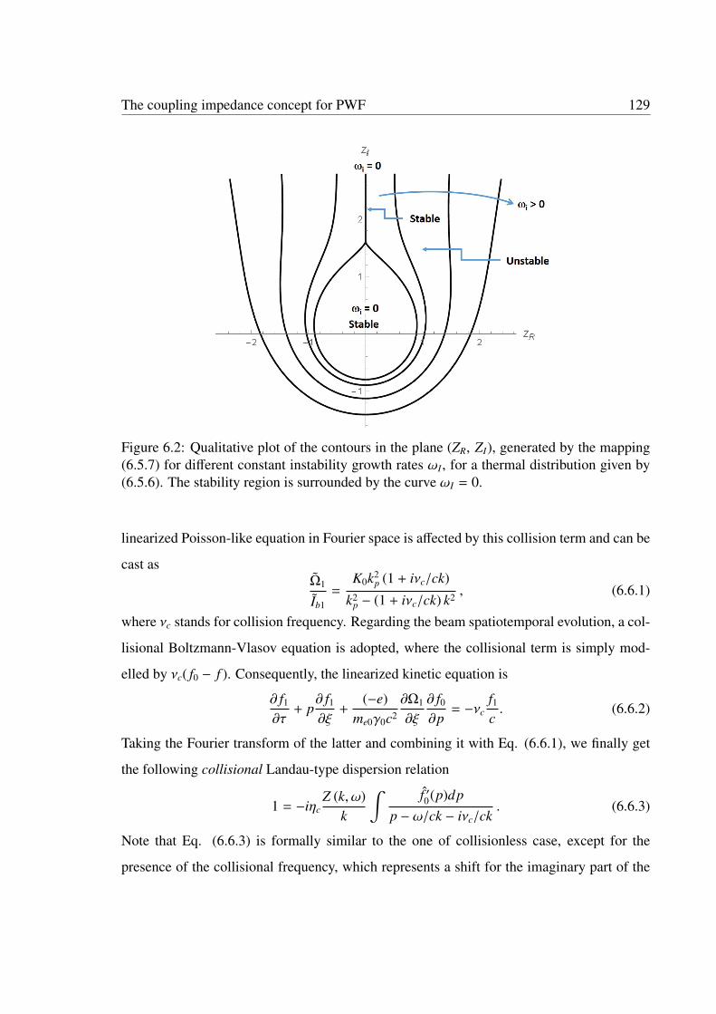
The coupling impedance concept for PWF 129
Figure 6.2: Qualitative plot of the contours in the plane (ZR, ZI), generated by the mapping(6.5.7) for different constant instability growth rates ωI , for a thermal distribution given by(6.5.6). The stability region is surrounded by the curve ωI = 0.
linearized Poisson-like equation in Fourier space is affected by this collision term and can be
cast asΩ1
Ib1=
K0k2p (1 + iνc/ck)
k2p − (1 + iνc/ck) k2 , (6.6.1)
where νc stands for collision frequency. Regarding the beam spatiotemporal evolution, a col-
lisional Boltzmann-Vlasov equation is adopted, where the collisional term is simply mod-
elled by νc( f0 − f ). Consequently, the linearized kinetic equation is
∂ f1
∂τ+ p
∂ f1
∂ξ+
(−e)me0γ0c2
∂Ω1
∂ξ
∂ f0
∂p= −νc
f1
c. (6.6.2)
Taking the Fourier transform of the latter and combining it with Eq. (6.6.1), we finally get
the following collisional Landau-type dispersion relation
1 = −iηcZ (k, ω)
k
∫ f ′0(p)dpp − ω/ck − iνc/ck
. (6.6.3)
Note that Eq. (6.6.3) is formally similar to the one of collisionless case, except for the
presence of the collisional frequency, which represents a shift for the imaginary part of the
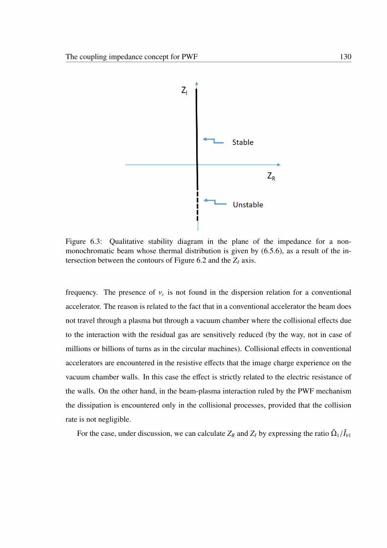
The coupling impedance concept for PWF 130
Figure 6.3: Qualitative stability diagram in the plane of the impedance for a non-monochromatic beam whose thermal distribution is given by (6.5.6), as a result of the in-tersection between the contours of Figure 6.2 and the ZI axis.
frequency. The presence of νc is not found in the dispersion relation for a conventional
accelerator. The reason is related to the fact that in a conventional accelerator the beam does
not travel through a plasma but through a vacuum chamber where the collisional effects due
to the interaction with the residual gas are sensitively reduced (by the way, not in case of
millions or billions of turns as in the circular machines). Collisional effects in conventional
accelerators are encountered in the resistive effects that the image charge experience on the
vacuum chamber walls. In this case the effect is strictly related to the electric resistance of
the walls. On the other hand, in the beam-plasma interaction ruled by the PWF mechanism
the dissipation is encountered only in the collisional processes, provided that the collision
rate is not negligible.
For the case, under discussion, we can calculate ZR and ZI by expressing the ratio Ω1/Ib1

The coupling impedance concept for PWF 131
with Eq. (6.4.1) and separating real and imaginary parts. This way, we get
ZR =νc
c
K0k4p
(−k2 + k2p)2 + ν2
ck2/c2 , (6.6.4)
ZI = −K0k2
p
[(−k2 + k2
p) − ν2c/c
2]
(−k2 + k2p)2 + ν2
ck2/c2 k . (6.6.5)
Therefore, the collisions introduce a resistance which now plays a role in the beam-plasma
dynamics. Note that in the limit νc → 0, Eqs. (6.6.4) and (6.6.5) recover Eqs. (6.5.2). In
addition, it should be emphasised that the collisions affect also the imaginary part of the
impedance and this is another important difference with respect to the conventional acceler-
ators. For brevity, we do not present here the stability analysis for the collisional case, but
the approach is fully similar to the one presented in section 6.5, except for the additional role
played by νc.
6.7 Conclusions
We have put forward the concept of coupling impedance that schematizes the self consistent
beam-plasma interaction ruled by the PWF excitation. We have emphasised similarity and
differences in comparison to the concept of coupling impedance in conventional accelerators.
We have illustrated with simple examples the role of the coupling impedance in the approach
to coherent beam-plasma instabilities. We have also outlined the interplay between Landau
damping and instability. An exhaustive and more rigorous approach which opens up to
important physical aspects, both energetic and collisional, is under way.
We would like to point out that the conditions of stability/instability discussed in section
6.5.1 and summarized in Table 6.1, have some similarities with the ones of monochromatic
coasting beam in the conventional accelerators. In particular, the possibility to combine the
sign of ZI with the sign of k fixes two symmetric conditions of instability that resemble the
ones of positive and negative mass instability, respectively. In conventional accelerators,
ZI > 0 and ZI < 0 correspond to impedances dominated by inductive and capacitive charac-
ters, respectively. The interplay between these impedance characters and the sign of the slip

The coupling impedance concept for PWF 132
factor [64] leads to the coherent instability conditions. Compare to the latter, the stability
conditions obtained in this work carry a little different meaning. In fact, the analog of the
negative mass instability seems to be associated with the case of k < 0 and ZI > 0, displayed
in Table 6.1. But here, the unstable evolution of a beam density/current perturbation appears
when the latter is propagating backward (and therefore, associated to some negative momen-
tum/energy). This and several other aspects of the beam-plasma instability, resulting from
the self-consistent PWF excitation, such as the physical condition of positive and negative
coupling impedance in connection with their inductive or capacitive character, and the exten-
sion of the coupling impedance in PWF accelerators to the transverse case, will be deepen in
a forthcoming work.
As a final remark we point out that a sensitive momentum (and thus energy) spread,
typical of beams accelerated injected in plasmas [80], could in principle stabilize the beam
itself by Landau damping, as described in this Section; such stabilization can only occur
provided that the growth rate of the instability that is inducing the momentum spread is
lower than the damping rate. Further work is necessary to study the interaction between
such kind of instabilities and Landau damping in the beam.

Conclusions and Remarks
We have carried out a theoretical investigation on the self-modulated dynamics that takes
place when a nonlaminar, relativistic, charged particle beam is travelling through a magne-
tized plasma while experiencing a strong interaction with the latter. This has been accom-
plished by developing the kinetic theory of the plasma wake field excitation. While trav-
elling, the beam experiences the strong electromechanical actions of the self consistent EM
fields of beam-plasma system that affect the beam envelope evolution. In this framework, the
pair of the 3D Vlasov-Poisson-type equations has been derived in the unperturbed particle
reference system. These equations governs the spatiotemporal evolution of the beam. We
have specialized this system of equations to a 2D purely transverse system and to a 1D purely
longitudinal system to describe the transverse and the longitudinal dynamics, respectively.
In the transverse dynamics, we have implemented the 2D Vlasov-Poisson-type equa-
tions for a cylindrically symmetric driving beam with the related virial equations. This has
allowed us to find some constant of motions and to obtain ordinary differential equations
for the time evolution of the beam spot size (envelope equations), that have been easily inte-
grated analytically and/or numerically. The use of the method of pseudo potential or Sagdeev
potential has been very helpful to carry out a qualitative analysis of the beam envelope self-
modulation. On the basis of such method, we have first carried out our analysis in the two
limiting cases of local (the beam spot size is much greater than the plasma wavelength) and
strongly non-local regimes (the beam spot size is much smaller than the plasma wavelength).
We have described several types of self-modulations, in terms of focusing, defocusing and
betatron-like oscillations, and have obtained the criteria for instability, such as collapse and
self-modulation instability. The analysis has been, then, extended to the general case where
133

Conclusions and Remarks 134
the beam spot size and the plasma wavelength are not necessarily constrained as in the lo-
cal or strongly nonlocal regimes. In these conditions, we have performed a semi-analytical
and numerical analysis of the envelope self-modulated dynamics and criteria for predicting
stability and self-modulation instability have been suitably provided.
In the longitudinal dynamics, we have used the Landau approach to the longitudinal
Vlasov-Poisson-type pair of equations. In fact, after linearizing this system around an un-
perturbed state, and taking the Fourier transformation of the resulting equation, we have
obtained a set of algebraic equation in frequency and wave number domain. From the lat-
ter, we have easily found the Landau-type dispersion relation. By using the latter, in the
monochromatic beam case, we have shown the existence of a purely growing mode and a
simple stability criterion. Then, by taking into account a non-monochromatic beam (de-
scribing a slightly warm beam), the Landau approach has lead to obtain both the dispersion
relation for the real part (showing all the possible beam modes in the diverse regions of the
wave number) and an expression for the imaginary part of the frequency, which has sug-
gested a simple stability criterion.
Within the context of the longitudinal beam dynamics, we have also introduced the novel
concept of coulpling impedance in plasma wake field accelerators in a way that is fully
similar to the one introduced in conventional particle accelerators. Based on the Landau-
type dispersion relation and the methods of Nyquist control theory, we have put forward an
alternative way to describe the coherent instabilities in the beam-plasma interaction.
In conclusion, the results we have obtained can be summarized as follows:
• We have developed the kinetic theory of the PWF excitation that provides the gener-
alized Vlasov-Poisson-type pair of equations for the diverse conditions of plasma and
beam;
• We have provided the self-modulated beam dynamics analysis in both purely trans-
verse and purely longitudinal cases;
• We have provided a satisfactory model for the self-modulation instability in the trans-
verse case, by implementing the Vlasov-Poisson-type equations with the related virial

Conclusions and Remarks 135
description (envelope equations);
• We have carried out an instability analysis within the linearized kinetic theory of the
self-consistent beam-plasma interaction, in the purely longitudinal case within two
approaches based on Landau theory.
Appendix A
Virial descriptions
Virial description is a method to integrate the single particle motion equation (i.e., Vlasov
equation) of a statistical system of charged particle beam, where the beam optics is described
in terms of root mean square (rms) beam moments and their respective equations of motion.
This method leads to find a set of equations, usually referred to as the virial equations for the
system of N particles bounded by a potential. Virial equations relate the average of the total
kinetic energy which comes from the kinetic description once the average of certain physical
quantities are taken by means of the distribution function.
Let us consider the transverse dynamics of a relativistic charged particle electron/positron
beam into a cold, Magnetized plasma. The beam is travelling along the z− axis with velocity
βc (β ' 1) in the presence of an external magnetic field (B0 = zB0). The motion of each
single particle is associated with an unperturbed total energy mb0γ0c2 (mb0 and γ0 being the
particle rest mass and the unperturbed relativistic factor, respectively). In the unperturbed-
particle frame, the transverse motion of each single-particle is associated with an effective
Hamiltonian, i.e., H (r⊥,p⊥, τ), i.e.,
H (r⊥,p⊥, τ) =12
p2⊥ +
12
kc z · (r⊥ × p⊥) +12
Kr2⊥ + Uw (r⊥, τ) , (A.0.1)
where Uw is the normalized plasma wake potential, K =(qB0/2mb0γ0c2
)2= (kc/2)2, kc =
−qB0/mb0γ0c2, r⊥ and p⊥ are the transverse component of position vector r and correspond-
ing conjugate momentum p. We can cast the above mentioned equation as:
H (r⊥,p⊥, τ) = T (p⊥) + U(r⊥,p⊥, τ) , (A.0.2)
136
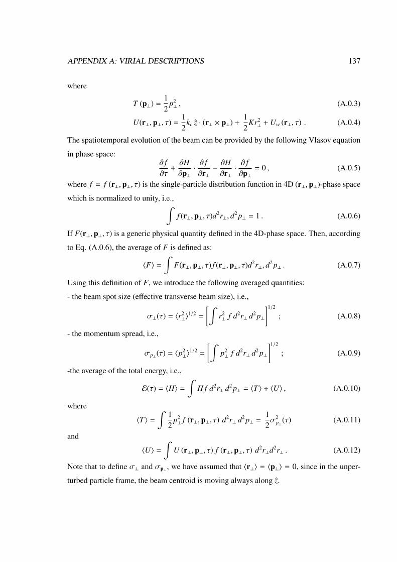
APPENDIX A: VIRIAL DESCRIPTIONS 137
where
T (p⊥) =12
p2⊥ , (A.0.3)
U(r⊥,p⊥, τ) =12
kc z · (r⊥ × p⊥) +12
Kr2⊥ + Uw (r⊥, τ) . (A.0.4)
The spatiotemporal evolution of the beam can be provided by the following Vlasov equation
in phase space:∂ f∂τ
+∂H∂p⊥·∂ f∂r⊥−∂H∂r⊥·∂ f∂p⊥
= 0 , (A.0.5)
where f = f (r⊥,p⊥, τ) is the single-particle distribution function in 4D (r⊥,p⊥)-phase space
which is normalized to unity, i.e.,∫f (r⊥,p⊥, τ)d2r⊥, d2 p⊥ = 1 . (A.0.6)
If F(r⊥,p⊥, τ) is a generic physical quantity defined in the 4D-phase space. Then, according
to Eq. (A.0.6), the average of F is defined as:
〈F〉 =
∫F(r⊥,p⊥, τ) f (r⊥,p⊥, τ)d2r⊥, d2 p⊥ . (A.0.7)
Using this definition of F, we introduce the following averaged quantities:
- the beam spot size (effective transverse beam size), i.e.,
σ⊥(τ) = 〈r2⊥〉
1/2 =
[∫r2⊥ f d2r⊥ d2 p⊥
]1/2
; (A.0.8)
- the momentum spread, i.e.,
σp⊥(τ) = 〈p2⊥〉
1/2 =
[∫p2⊥ f d2r⊥ d2 p⊥
]1/2
; (A.0.9)
-the average of the total energy, i.e.,
E(τ) = 〈H〉 =
∫H f d2r⊥ d2 p⊥ = 〈T 〉 + 〈U〉 , (A.0.10)
where
〈T 〉 =
∫12
p2⊥ f (r⊥,p⊥, τ) d2r⊥ d2 p⊥ =
12σ2
p⊥(τ) (A.0.11)
and
〈U〉 =
∫U (r⊥,p⊥, τ) f (r⊥,p⊥, τ) d2r⊥d2r⊥ . (A.0.12)
Note that to define σ⊥ and σp⊥ , we have assumed that 〈r⊥〉 = 〈p⊥〉 = 0, since in the unper-
turbed particle frame, the beam centroid is moving always along z.
APPENDIX A: VIRIAL DESCRIPTIONS 138
First virial equation
We are going to derive an evolution equation for σ2⊥(τ). Therefore, we first differentiate the
square of Eq. (A.0.8) with respect to τ, i.e.,
dσ2⊥
dτ=
∫r2⊥
∂ f∂τ
d2r⊥ d2 p⊥ . (A.0.13)
Using Eq. (A.0.5), we substitute ∂ f /∂r⊥ in Eq. (A.0.13), and get,
dσ2⊥
dτ= −
∫r2⊥
[∂H
∂p⊥·∂ f∂r⊥−∂H
∂r⊥·∂ f∂p⊥
]d2r⊥ d2 p⊥ . (A.0.14)
This equation can be written as,
dσ2⊥
dξ= −
∫r2⊥
∂H
∂p⊥·∂ f∂r⊥
d2r⊥ d2 p⊥ +
∫r2⊥
∂H
∂r⊥·∂ f∂p⊥
d2r⊥ d2 p⊥ . (A.0.15)
To evaluate the first integral in the left-hand side of Eq. (A.0.15), at first we take the diver-
gence of the quantity r2⊥ (∇p⊥H) f ,
∇⊥ ·[r2⊥(∇p⊥H) f
]= 2r⊥ · (∇p⊥H) f + r2
⊥∇⊥ · (∇p⊥H) f + r2⊥(∇p⊥H) · (∇⊥ f ) (A.0.16)
or,
r2⊥
∂H
∂p⊥·∂ f∂r⊥
= ∇⊥ ·
[r2⊥
∂H
∂p⊥f]− 2r⊥ ·
∂H
∂p⊥f − r2
⊥∇⊥ · (∇p⊥H) f . (A.0.17)
Taking integration of (A.0.17), we get,∫r2⊥
∂H
∂p⊥·∂ f∂r⊥
d2r⊥ d2 p⊥ =
∫∇⊥ ·
[r2⊥
∂H
∂p⊥f]
d2r⊥ d2 p⊥ − 2∫
r⊥ ·∂H
∂p⊥f d2r⊥ d2 p⊥
−
∫r2⊥∇⊥ · (∇p⊥H) f d2r⊥ d2 p⊥ . (A.0.18)
At the infinity the first integration of the right-hand side of Eq. (A.0.18) goes to zero and
after using Eq. (A.0.18) into (A.0.15), we get
−
∫r2⊥
∂H
∂p⊥·∂ f∂r⊥
d2r⊥ d2 p⊥ = 2⟨r⊥ · ∇p⊥H
⟩+
⟨r2⊥∇⊥ · (∇p⊥H)
⟩. (A.0.19)
The second integral in the right-hand side of Eq. (A.0.15) can be written as,∫r2⊥
∂H
∂r⊥·∂ f∂p⊥
d2r⊥ d2 p⊥ = −⟨r2⊥∇p⊥ · (∇⊥H)
⟩. (A.0.20)

APPENDIX A: VIRIAL DESCRIPTIONS 139
Using Eqs. (A.0.19) and (A.0.20) into Eq. (A.0.15), we get:
dσ2⊥
dτ= 2
⟨r⊥ · ∇p⊥H
⟩+
⟨r2⊥
[∇⊥ · (∇p⊥H) − ∇p⊥ · (∇⊥H)
]⟩. (A.0.21)
By taking the derivatives of Hamiltonian given in Eq. (A.0.1) with respect to p⊥ and r⊥, we
get,
∇p⊥H =∂H∂p⊥
= p⊥ +12
kc(z × r⊥) (A.0.22)
and
∇⊥H =∂H∂r⊥
= Kr⊥ + ∇⊥Uw −12
kc(z × p⊥) . (A.0.23)
Taking the scalar products of Eq. (A.0.22) with respect to ∇⊥ and of Eq. (A.0.23) with
respect to ∇p⊥ , respectively, we get,
∇⊥ · (∇p⊥H) = ∇⊥ ·
[p⊥ +
12
kc(z × r⊥)]
= 0 (A.0.24)
and
∇p⊥ · (∇⊥H) = ∇p⊥ ·
[Kr⊥ +
∂Uw
∂r⊥−
12
kc(z × p⊥)]
= 0 . (A.0.25)
Using Eqs. (A.0.24) and (A.0.25), we see that the second term at the right-hand side of Eq.
(A.0.21) vanishes; therefore this equation becomes
dσ2⊥
dτ= 2 〈r⊥ · p⊥〉 = 2
∫(r⊥ · p⊥) f d2r⊥ d2 p⊥ , (A.0.26)
which can be also cast as
σ⊥dσ⊥dτ
= 〈r⊥ · p⊥〉 . (A.0.27)
We take the derivative of Eq. (A.0.26),
d2σ2⊥
dτ2 = 2∫
(r⊥ · p⊥)∂ f∂τ
d2r⊥ d2 p⊥ . (A.0.28)
Then, we obtain ∂ f /∂τ from Eq. (A.0.5) and substitute into (A.0.28),
d2σ2⊥
dτ2 = −2∫
(r⊥ · p⊥)[∂H
∂p⊥·∂ f∂r⊥−∂H
∂r⊥·∂ f∂p⊥
]d2r⊥ d2 p⊥ (A.0.29)
or,
d2σ2⊥
dτ2 = −2∫
(r⊥ · p⊥)∂H
∂p⊥·∂ f∂r⊥
d2r⊥ d2 p⊥ + 2∫
(r⊥ · p⊥)∂H
∂r⊥·∂ f∂p⊥
d2r⊥ d2 p⊥ . (A.0.30)

APPENDIX A: VIRIAL DESCRIPTIONS 140
Following the similar procedure to reach Eqs. (A.0.19) and (A.0.20), the integrals in the
right-hand side of (A.0.30) can be expressed as,
− 2∫
(r⊥ · p⊥)∂H
∂p⊥·∂ f∂r⊥
d2r⊥ d2 p⊥ = 2⟨p⊥ · ∇p⊥H
⟩+ 2
⟨(r⊥ · p⊥)∇⊥ · (∇p⊥H)
⟩(A.0.31)
and
2∫
(r⊥ · p⊥)∂H
∂r⊥·∂ f∂p⊥
d2r⊥ d2 p⊥ = −2 〈r⊥ · ∇⊥H〉 . (A.0.32)
Using Eqs. (A.0.31) and (A.0.32) into (A.0.30), we get
d2σ2⊥
dτ2 = 2⟨p⊥ · ∇p⊥H
⟩+ 2
⟨(r⊥ · p⊥)∇⊥ · (∇p⊥H)
⟩− 2 〈r⊥ · (∇⊥H)〉 . (A.0.33)
Then, taking dot product of p⊥ and r⊥ with Eqs. (A.0.24) and (A.0.25), respectively, we get
p⊥ · ∇p⊥H = p2⊥ +
12
kcp⊥ · (z × r⊥) , (A.0.34)
r⊥ · ∇⊥H = Kr2⊥ + r⊥ · ∇⊥Uw −
12
kcr⊥ · (z × p⊥) . (A.0.35)
Furthermore, we observe that,
∇⊥ · (∇p⊥H) = ∇⊥ ·
[p⊥ +
12
kc(z × r⊥)]
= 0 . (A.0.36)
Using Eqs. (A.0.34) - (A.0.36) into (A.0.33), we finally obtain:
d2σ2⊥
dτ2 = 2⟨p2⊥
⟩+ kc〈p⊥ · (z × r⊥)〉 − 2K〈r2
⊥〉 − 2〈r⊥ · ∇⊥Uw〉 + kc〈r⊥ · (z × p⊥)〉 ,
which can be expressed as
d2σ2⊥
dτ2 = 2σ2p⊥ − 2Kσ2
p⊥ − 2〈r⊥ · ∇⊥Uw〉 + kc〈z · (r⊥ × p⊥) + z · (p⊥ × r⊥)〉 . (A.0.37)
We observe that the sum of the last two terms of Eq. (A.0.37) is zero, i.e., z · (r⊥ × p⊥) + z ·
(p⊥ × r⊥) = 0, hence, we get,
d2σ2⊥
dτ2 = 2σ2p⊥ − 2Kσ2
p⊥ − 2〈r⊥ · ∇⊥Uw〉 . (A.0.38)
In terms of T and V , Eq. (A.0.38) can be written as,
d2σ2⊥
dτ2 = 4〈T 〉 − 2〈r⊥ · ∇⊥V〉 , (A.0.39)

APPENDIX A: VIRIAL DESCRIPTIONS 141
where,
V(r⊥, τ) =12
Kr2⊥ + Uw(r⊥, τ) . (A.0.40)
Equation (A.0.39) is referred to be the first virial equation. It can be consequently cast in the
following form,d2σ2
⊥
dτ2 = 2σ2p⊥ − 2Kσ2
⊥ − 2〈r⊥ · ∇⊥Uw〉 (A.0.41)
or,d2σ2
⊥
dτ2 = 4(E − 〈U〉) − 2〈r⊥ · ∇r⊥U〉 + kcLz , (A.0.42)
where Lz = 〈Lz〉, Lz = z · (r⊥ × p⊥), and U is given in Eq. (A.0.4). In case of unmagnetized
plasma, the first virial equation becomes (kc = K = 0):
d2σ2⊥
dτ2 = 4(E − 〈Uw〉) − 2〈r⊥ · ∇r⊥Uw〉 , (A.0.43)
where E = 12 〈p
2⊥〉 + 〈Uw〉. In order to close the virial description, we need the second virial
equation which will relate E with Uw.
Second virial equation
Now we are going to find an equation for the time evolution of the averaged total energy
E(τ) = 〈H〉 which is defined in Eq. (A.0.10). To do this, we differentiate Eq. (A.0.10) with
respect to τ, obtaining
dEdτ
=
∫∂H∂τ
f d2 p⊥d2r⊥ +
∫H∂ f∂τ
d2 p⊥d2r⊥ , (A.0.44)
which, by using Eq. (A.0.5) can be cast as:
dEdτ
=
⟨∂H∂τ
⟩−
∫H
[∂H∂p⊥·∂ f∂r⊥−∂H∂r⊥·∂ f∂p⊥
]d2 p⊥d2r⊥ . (A.0.45)
The last term of Eq. (A.0.45) can be written as,
H[∂H∂p⊥·∂ f∂r⊥−∂H∂r⊥·∂ f∂p⊥
]=
H2
(∂H2
∂p⊥·∂ f∂r⊥−∂H2
∂r⊥·∂ f∂p⊥
). (A.0.46)
We can write the following derivatives as,
∇⊥
[∂H2
∂p⊥f]
=∂H2
∂p2⊥
∂ f∂r⊥
+ f∇⊥(∇p⊥H2) (A.0.47)
APPENDIX A: VIRIAL DESCRIPTIONS 142
and
∇p⊥
[∂H2
∂r⊥f]
=∂H2
∂r⊥∂ f∂p⊥
+ f∇p⊥(∇r⊥H2) . (A.0.48)
Using Eqs. (A.0.47) and (A.0.48) into Eq. (A.0.46) while using the boundary condition atinfinity, the last integral of Eq. (A.0.45) becomes,∫
H[∂H∂p⊥
·∂ f∂r⊥−∂H∂r⊥·∂ f∂p⊥
]d2 p⊥d2r⊥ =
∫f[∇⊥ · (H∇p⊥H) − ∇p⊥ · (H∇⊥H)
]d2 p⊥d2r⊥ ,
or,∫H
[∂H∂p⊥
·∂ f∂r⊥−∂H∂r⊥·∂ f∂p⊥
]d2 p⊥d2r⊥ =
∫f[H
∂
∂xi
(∂H∂pi
)− H
∂
∂p j
(∂H∂x j
)]d2 p⊥d2r⊥ ,
or,∫H
[∂H∂p⊥
·∂ f∂r⊥−∂H∂r⊥·∂ f∂p⊥
]d2 p⊥d2r⊥ =
∫f[H
[∂2H∂xi∂pi
−∂2H∂p j∂x j
]]d2 p⊥d2r⊥ = 0 .(A.0.49)
Using Eq. (A.0.49) into Eq. (A.0.45), we get
dEdτ
=
⟨∂Uw
∂τ
⟩=
∫∂UW
∂τf d2r⊥d2 p⊥ , (A.0.50)
where we have used the explicit form of H given by Eq. (A.0.1) and observed that Uw(r⊥, τ)
is the only term of the Hamiltonian that depends explicitly on τ.
We refer Eq. (A.0.50) to be the second virial equation, which describes the time evolution
of the averaged energy E. Equations (A.0.39) and (A.0.50) constitute a pair of coupled
equations governing the time evolution of the beam envelope.
Appendix B
Envelope descriptions
To give a complete self-consistent description of the beam plasma system, along with the
two virial equations (A.0.39) and (A.0.50) described in the Appendix A, the knowledge of f
and Uw is required. Therefore, equations (A.0.39) and (A.0.50) do not comprise a complete
set of equations. To satisfy the self-consistency, we have to couple the Vlasov-Poisson-type
system of equations with equations with (A.0.39) and (A.0.50). Imposing suitable initial
and boundary conditions, we have to solve the Vlasov-Poisson-type pair of equations. Once
f (r⊥,p⊥, τ) and Uw(r⊥, τ) are known, we can use the virial equations to describe the time
evolution of the beam envelope.
We take into account the following Vlasov-Poisson-type pair of equations,
∂ f∂τ
+
[p⊥ +
12
kc (z × r⊥)]· ∇⊥ f −
[Kr⊥ −
12
kc (z × p⊥) + ∇⊥Uw
]· ∇p⊥ f = 0 , (B.0.1)
(∇2⊥ − k2
s
)Uw = k2
sλ0
∫f d2 p⊥ , (B.0.2)
where λ0 = N/n0γ0σz (N being the total number of electrons or positrons of the driving
beam) and ks = k2p/kuh. Since Uw is independent of p⊥, from Eq. (A.0.50) we get,
dEdτ
=
∫∂UW
∂τd2r⊥
∫f d2 p⊥ . (B.0.3)
Using Eqs. (B.0.2) and (B.0.3), we get:
dEdτ
=1
k2sλ0
[ ∫∂Uw
∂τ∇2⊥Uw d2r⊥ − k2
s
∫Uw
∂Uw
∂τd2r⊥
]. (B.0.4)
143

APPENDIX B: ENVELOPE DESCRIPTIONS 144
To evaluate the first integral in the left-hand side of Eq. (B.0.4), at first we take the divergence
of the (∂Uw)/(∂τ)∇⊥Uw,
∇⊥ ·
[∂Uw
∂τ∇⊥Uw
]=
(∇⊥
∂Uw
∂τ
)· ∇⊥Uw +
∂Uw
∂τ∇2⊥Uw ,
which in turn gives,
∂Uw
∂τ∇2⊥Uw = ∇⊥ ·
[∂Uw
∂τ∇⊥Uw
]−
12∂
∂τ|∇⊥Uw|
2 . (B.0.5)
Using Eq. (B.0.5) into Eq. (B.0.4), we get
dEdτ
=1
k2sλ0
[ ∫∇⊥ ·
(∂Uw
∂τ∇⊥Uw
)d2r⊥ −
12
∫∂
∂τ|∇⊥Uw|
2 d2r⊥ − k2s
∫12∂U2
w
∂τd2r⊥
]. (B.0.6)
At the infinity the first integration of the right-hand side of Eq. (B.0.6) goes to zero. There-
fore, we get,dEdτ
= −1
2k2sλ0
ddτ
∫ (|∇⊥Uw|
2 + k2sU2
w
)d2r⊥ , (B.0.7)
or,ddτ
[E +
12k2
sλ0
∫ (|∇⊥Uw|
2 + k2sU2
w
)d2r⊥
]= 0 . (B.0.8)
Consequently, from this equation we can define the following constant of motion:
C = E +1
2k2sλ0
∫ (|∇⊥Uw|
2 + k2sU2
w
)d2r⊥ . (B.0.9)
By expressing explicitly E = 〈H〉 along with Eqs. (A.0.2) - (A.0.4) in the above equation,
we easily get:
C =12σ2
p⊥ +12
Kσ2⊥ +
12k2
sλ0
∫ (|∇⊥Uw|
2 + k2sU2
w
)d2r⊥ + 〈Uw〉 +
12
kcLz . (B.0.10)
Then, using 〈Uw〉, i.e.,
〈Uw〉 = −1
k2sλ0
∫ (|∇⊥Uw|
2 + k2sU2
w
)d2r⊥ , (B.0.11)
into Eq. (B.0.10), we get
C =12σ2
p⊥ +12
Kσ2⊥ −
12k2
sλ0
∫ (|∇⊥Uw|
2 + k2sU2
w
)d2r⊥ +
12
kcLz . (B.0.12)

APPENDIX B: ENVELOPE DESCRIPTIONS 145
By means of Eq. (B.0.12), we express E in terms of C and substitute it in the first virial
equation. Then, using Eqs. (B.0.12) and (A.0.4) into Eq. (A.0.42) we easily get:
d2σ2⊥
dτ2 + 4 Kσ2⊥ = 4C −
2k2
sλ0
∫ (|∇⊥Uw|
2 + k2sU2
w
)d2r⊥ − 4〈Uw〉 − 2〈r⊥ · ∇⊥Uw〉 − 2kcLz .
(B.0.13)
After performing the integrations by parts, contained in the terms at the right-hand side of
Eq. (B.0.13), we finally obtain the following envelope equation, i.e.,
d2σ2⊥
dτ2 + 4 Kσ2⊥ = 4C +
2k2
sλ0
∫|∇⊥Uw|
2 d2r⊥ − 2kcLz . (B.0.14)
Note that, for the case of unmagnetized plasma (B0 = 0), we easily get:
d2σ2⊥
dτ2 = 4C +2
k2pλ0
∫|∇⊥Uw|
2 d2r⊥ . (B.0.15)
List of Publications/Communications
International publications
R. Fedele, T. Akhter, D. Jovanovic, S. De Nicola, and A. Mannan, Transverse evolution of a
long relativistic electron beam governed by the Vlasov-Poisson-type pair of equations within
the plasma wake field dynamics in the local regime, Eur. Phys. J. D 68, 210 (2014). DOI:
10.1140/epjd/e2014-50219-y
R. Fedele, A. Mannan, S. De Nicola, D. Jovanovic, and T. Akhter, Vlasov’s kinetic theory of
the collective charged particle beam transport through a magnetized plasma in the strongly
nonlocal regime, Eur. Phys. J. D, 68, 271 (2014). DOI: 10.1140/epjd/e2014-50220-6
R. Fedele, T. Akhter, S. De Nicola, M. Migliorati, A. Marocchino, F. Massimo, and L.
Palumbo, The concept of coupling impedance in the self-consistent plasma wake field exci-
tation, Nucl. Instr. Meth. A, Accepted, (2015).
T. Akhter, R. Fedele, S. De Nicola, F. Tanjia, D. Jovanovic, and A. Mannan, Self-modulated
dynamics of a relativistic charged particle beam in plasma wake field excitation, Nucl. Instr.
Meth. A, Submitted (2015).
F. Tanjia, R. Fedele, S. De Nicola, T. Akhter, and D. Jovanovic, Formation and stability
of a hollow electron beam in the presence of a plasma wake field driven by an ultra-short
electron bunch, Nucl. Instr. Meth. A, Revised, (2015).
F. Tanjia, R. Fedele, S. De Nicola, T. Akhter, D. Jovanovic, Formation of stable hollow
electron beam by external injection in a plasma wake field accelerator, Phys. Rev. A. B.,
Submitted, (2015).
146

List of Publications/Communications 147
Poster Presentations
1. T. Akhter, R. Fedele, S. De Nicola, F. Tanjia, D. Jovanovic, Study of the self-modulated
propagation of relativistic charged particle beam in warm-magnetized plasmas within
the kinetic description, FISMAT 2015, 28 September - 02 October, 2015, Plalermo,
Italy
2. T. Akhter, R. Fedele, A. Mannan, S. De Nicola and F. Tanjia, Dynamics of a Self-
Modulated Relativistic Charged Particle Beam in a Plasma, International Congress
On Plasma Physics ICPP 2014, 15 - 19 September 2014, Lisbon, Portugal.
3. T. Akhter, R. Fedele, A. Mannan, S. De Nicola and F. Tanjia, Dynamics of a Self-
Modulated Relativistic Charged Particle Beam in a Plasma, Joint ICTP-IAEA College
on Advanced Plasma Physics, 18 - 29 August 2014, ICTP, Trieste, Italy.
4. R. Fedele, S. De Nicola, T. Akhter, A. Mannan, F. Tanjia and D. Jovanovic, Quantum-
like aspects of the charged-particle beam self-modulation in the presence of a laser
wake field excitation, School on Non-linear Dynamics, Dynamical Transitions and
Instabilities in Classical and Quantum Systems, ICTP, 14 July - 1 August 2014, Trieste,
Italy.
5. A. Mannan, R. Fedele, S. De Nicola, D. Jovanovic, and T. Akhter, Collective trans-
port of a charged particle beam through an unmagnetized plasma within the frame-
work of the Vlasovs kinetic theory in strongly nonlocal regime, VLASOVIA 2013,
International workshop on the theory and applications of Vlasov equation, 25 - 28
November 2013, Nancy, France.
6. T. Akhter, R. Fedele, S. De Nicola, D. Jovanovic, and A. Mannan, Analysis of the
transverse plasma wake field dynamics of a long relativistic electron beam governed
by the Vlasov-Poisson-like pair of equations in purely local regime, VLASOVIA 2013,
International workshop on the theory and applications of Vlasov equation, 25 - 28
November 2013, Nancy, France.

List of Publications/Communications 148
Oral Presentations
1. T. Akhter, R. Fedele, A. Mannan, S. De Nicola, and F. Tanjia Self-Modulated Rela-
tivistic Charged Particle Beam dynamics in a Plasma, 100 Congresso Nazionale SIF,
22 - 26 September 2014, Pisa, Italy.
2. T. Akhter, R. Fedele, S. De Nicola, D. Jovanovic, and A. Mannan Stabilizing Effects
in a Self-Modulated Long Relativistic Charged Particle Beam Travelling in a Plasma,
Trieste, Italy.
3. T. Akhter, R. Fedele, S. De Nicola, F. Tanjia, D. Jovanovic, Self modulated dynamics
of relativistic charged particle beam in plasma wake field excitation, La Biodola, Isola
dElba, Italy, 13-19 September, 2015.
4. T. Akhter, R. Fedele, S. De Nicola, F. Tanjia, D. Jovanovic, Kinetic theory of the gen-
eralized self-consistent 3D plasma wake field excitation in overdense regime, Roma,
Italy, 21-25 September, 2015.
International conferences & visits
1. 2nd European Advanced Accelerator Concepts Workshop, La Biodola, Isola dElba,
Italy, 13-19 September, 2015.
2. 101 Congresso Nazionale, Societa Italiana di Fisica, Roma, Italy, 21-25 September,
2015.
3. 100 Congresso Nazionale SIF, 22 - 26 September 2014, Pisa, Italy.
4. International Congress On Plasma Physics ICPP 2014, 15 - 19 September 2014, Lis-
bon, Portugal.
5. Joint ICTP-IAEA College on Advanced Plasma Physics, 18 - 29 August 2014, ICTP,
Trieste, Italy.
List of Publications/Communications 149
6. VLASOVIA 2013, International workshop on the theory and applications of Vlasov
equation, 25 - 28 November 2013, Nancy, France.
Bibliography
[1] T. Tajima and J. M. Dawson. Laser electron accelerator. Phys. Rev. Lett., 43:267–270,1979.
[2] L. M. Gorbunov and V. I. Kirsanov. Excitation of plasma waves by an electromagneticwave packet. Sov. Phys. JETP, 66:290–294, 1987.
[3] P. Sprangle, E. Esarey, A. Ting, and G. Joyce. Appl. Phys. Lett., 53:2146–2148, 1988.
[4] P. Chen, J. M. Dawson, R. W. Huff, and T. Katsouleas. Acceleration of electrons by theinteraction of a bunched electron beam with a plasma. Phys. Rev. Lett., 54:693–696,1985.
[5] R. D. Ruth, A. W. Chao, P. L. Morton, and P. B. Wilson. Part. Accel., 17:171, 1985.
[6] P. Chen, J. J. Su, J. M. Dawson, K. L. F. Bane, and P. B. Wilson. Phys. Rev. Lett.,56:1252, 1986.
[7] J. Rosenzweig. IEEE Trans. Plasma Science, PS-15:186, 1987.
[8] T. Katsouleas. Phys. Rev. A, 33:2056, 1986.
[9] R. Fedele, U. de Angelis, and T. Katsouleas. Generation of radial fields in the beat-waveaccelerator for gaussian pump profiles. Phys. Rev. A, 33:4412–4414, 1986.
[10] U. De Angelis, R. Fedele, G. Miano, and C. Nappi. Plasma Phys. Control. Fusion,29:789, 1987.
[11] C. Joshi, T. Katsouleas, J. M. Dawson, Y. T. Yan, and J. M. Slater. IEEE Trans. J.Quantum Electronics, QE-23:1571, 1987.
[12] R. Fedele, G. Miano, and V. G. Vaccaro. Physica Scripta, T30:192, 1990.
150

Bibliography 151
[13] A. O. Benz. Astrophys. J., 211:270, 1977.
[14] J. Kuijpers. ‘Particle acceleration’ in Plasma Astrophysics, Springer:Berlin, 1996.
[15] M. E. Dieckmann, P. Ljung, A. Ynnerman, and K. G. McClements. Phys. Plasmas,7:5171, 2000.
[16] K. G. McClements, R. O. Dendy, M. E. Dieckmann, A. Ynnerman, and S. C. Cha Pma.J. Plasma Physics, 71:127, 2005.
[17] P. Chen, T. Tajima, and Y. Takahashi. Phys. Rev. Lett., 89:161101, 2002.
[18] A. M. Sessler and D. Vaughan. Free-Electron Lasers. University of California, Berke-ley, 1987.
[19] H. Winick et al. Wiggler and undulator magnets. Phys. Today, 34N5:50–63, 1981.
[20] H. Winick. Synchrotron radiation. Scientific American, 255:88–89, 1987.
[21] J. M. Dawson. From Particles to Plasmas, page 131. Addison Wesley, Reading, MA,1959.
[22] J. M. Dawson. Nonlinear electron oscillations in a cold plasma. Phys. Rev.,113:383387, 1959.
[23] J. Faure, Y. Glinec, A. Pukhov, S. Kiselev, S. Gordienko, E. Lefebvre, J. P. Rousseau,F. Burgy, and V. Malka. Nature, 431:541, 2004.
[24] C. G. R. Geddes, Cs. Toth, J. Van Tilborg, E. Esarey, C. B. Schroeder, D. Bruh-wiler,C. Nieter, J. Cary, and W. P. Leemans. Nature, 431:538, 2004.
[25] S. P. D. Mangles et al. Monoenergetic beams of relativistic electrons from intenselaserplasma interactions. Nature, 431:535–538, 2004.
[26] J. Faure, C. Rechatin, A. Norlin, A. Lifschitz, Y. Glinec, and V. Malka. Nature,444:737, 2006.
[27] W. Leemans, B. Nagler, A. J. Gonsalves, Cs. Toth, K. Nakamura, C. G. R. Geddes,E. Esarey, C. B. Schroeder, and S. M. Hooker. Nat. Phys., 2:696, 2006.

Bibliography 152
[28] C. E. Clayton, J. E. Ralph, F. Albert, R. A. Fonseca, S. H. Glenzer, C. Joshi, W.Lu,K. A. Marsh, S. F. Martins, W. B. Mori, A. Pak, F.S. Tsung, B. B. Pollock, J. S. Ross,L. O. Silva, and D. H. Froula. Phys. Rev. Lett., 105:105003, 2010.
[29] K.A. Marsh, C. E. Clayton, C. Joshi, W. Lu, W. B. Mori, A. Pak, L. O. Silva, N. Lemos,R. A. Fonseca, S. de Freitas Martins, F. Albert, T. Doeppner, C. Filip, D. Froula, S. H.Glenzer, D. Price, J. Ralph, and B. B. Pollock. LLNLPROC, 476791, 2011.
[30] R. Bingham, J.T. Mendonca, and P.K. Shukla. Plasma based charged-particle acceler-ators. Plasma Phys. Control. Fusion, 46:R1–R23, 2004.
[31] D. Jovanovic, R. Fedele, F. Tanjia, S. De Nicola, and L. A. Gizzi. Eur. Phys. J. D,66:328, 2012.
[32] D. Jovanovic, R. Fedele, and M. Belic. Euro. phys. Let., 107:44004, 2014.
[33] A.V. Korzhimanov, A. Gonoskov, E. A Khazanov, and A. M Sergeev. Phys. Usp., 54:9,2011.
[34] X. Wang, R. Zgadzaj, N. Fazel, Z. Li, S. A. Yi, X. Zhang, W. Henderson, Y.-Y. Chang,R. Korzekwa, H.-E. Tsai, C.-H. Pai, H. Quevedo, G. Dyer, E. Gaul, M. Martinez, A. C.Bernstein, T. Borger, M. Spinks, M. Donovan, V. Khudik, G. Shvets, T. Ditmire, andM. C. Downer. Nature Communications, 4:1988, 2013.
[35] W. Lu nad C. Huang and M. Zhou et al. Phys. Plasmas, 13:056709, 2006.
[36] I. Kostyukov, A. Pukhov, and S. Kiselev. Phys. Plasmas, 11:5256, 2004.
[37] R. Bingham. Nature, 445:721, 2007.
[38] V. Malka, J. Faure, Y. A. Gauduel, E. Lefebvre, A. Rousse, and K.T. Phuoc. NaturePhysics, 4:447, 2008.
[39] P. Muggli and M. J. Hogan. Review of high-energy plasma wakefield experiments. C.R. Phys., 10:116–129, 2009.
[40] J.B. Rozenzweig, D.B. Cline, B. Cole, H. Figueroa, W. Gai, R. Konecny, J. Norem,P. Schoessow, and J. Simpson. Phys. Rev. Lett., 61:98–101, 1988.

Bibliography 153
[41] J. B. Rosenzweig, B. Breizman, T. Katsouleas, and J. J. Su. Acceleration and focusingof electrons in two-dimensional nonlinear plasma wake fields. Phys. Rev. A, 44:R6189–R6192, 1991.
[42] G. Xia, O. Mete, A. Aimidula, C. P. Welsch, S. Chattopadhay, S. Mandry, and M. Wing.Nucl. Instrum. Meth. A, 740:173, 2014.
[43] E. Oz and P. Muggli. Nucl. Instrum. Meth. A, 740:197, 2014.
[44] M. J. Hogan et al. New J. Phys., 12:055030, 2010.
[45] B. Marchetti, A. Bacci, E. Chiadroni, A. Cianchi, M. Ferrario, A. Mostacci,R. Pompili, C. Ronsivalle, B. Spataro, and I. Zagorodnov. Rev. Sci. Instrum.,7(10.1063/1.4922882):073301, 2015.
[46] A. B. Mikhailovskii. Plasma Phys., 22:133, 1980.
[47] V. N. Tsytovich. Sov. Phys. Doklady, 7:31, 1962.
[48] A. I. Akhiezer, I. A. Akhiezer, R. V. Polovin, A. G. Sitenko, and K. N. Stepanov.Plasma Electrodynamics, 2, 1975.
[49] A. A. Vlasov. On vibration properties of electron gas. J. Exp. Theor. Phys. (in Russian),8:3, 1938.
[50] D. R. Hartree. The calculation of Atomic Structures. John Wiley & Sons Ltd., NewYork, 1957.
[51] K. Huang. Statistical Mechanics. John Wiley & Sons Ltd., New York, 2 edition, 1987.
[52] A. I. Akhiezer, I. A. Akhiezer, R. V. Polovin, A. G. Sitenko, and K. N. Stepanov.Plasma Electrodynamics, 1, 1975.
[53] C. Castaldo, R. Fedele, U. de Angelis, and R. Bingham. Thermal effects in relativisticplasmas. First Course Int. School of Particle Accelerators of the ‘Ettore Majorana’ Cen-tre for Scientific Culture. RAL-90-082 November 1990; Proc. 10th European PlasmaPhysics Summer School, Tbilisi, 2-15 September, 2015. N.L. Tsintzadze (Ed.) (Worldscientific, Singapore, 1990) p. 371.
[54] Gerhard Rein. Comm. Math. Phys., 135:41, 1990.

Bibliography 154
[55] W. K. H. Panofsky and W. A. Wenzel. Some considerations concerning the transversedeflection of charged particles in radio-frequency fields. Rev. Sci. Instrum., 27:967,1956.
[56] R. Fedele, F. Tanjia, S. De Nicola, D. Jovanovic, and P.K. Shukla. Phys. Plasmas,19:102106, 2012.
[57] F. Tanjia, R. Fedele, S. De Nicola, T. Akhter, and D. Jovanovi. Phys. Rev. A. B. (Re-vised), 2015.
[58] R. Fedele, T. Akhter, D. Jovanovi, S. De Nicola, and A. Mannan. Eur. Phys. J. D,68:210, 2014.
[59] R. Fedele, A. Mannan, S. De Nicola, D. Jovanovi, and T. Akhter. Eur. Phys. J. D,68:271, 2014.
[60] T. Akhter, R. Fedele, S. De Nicola, F. Tanjia, and D. Jovanovi. Nucl. Instr. Meth. A(Revised), 2015.
[61] R. Fedele, D. Jovanovi, S. De Nicola, A. Mannan, and F. Tanjia. Journal of Physics:Conference Series, 482:012014, 2014.
[62] R. Fedele, D. Jovanovi, F. Tanjia, and S. De Nicola. Nuclear Instruments and Methodsin Physics Research A, 740:180, 2014.
[63] J. D. Jackson. Classical Electrodynamics, Second Edition. John Wiley and Sons, 1975.
[64] J. D. Lawson. The Physics of Charged-Particle Beams. Clarendon Press, Oxford, 2ndedition, 1988.
[65] S. Humphies. Principles of Charged Particle Acceleration. John Wiley and Sons, 1999.
[66] L. D. Landau. J. Phys. USSR 10, 25, 1946.
[67] F. F.Chen. Introduction to plasma physics and controlled fusion. Plenum Press, NewYork, 2 edition, 1984.
[68] R. Fedele and D. Anderson. A quantum-like landau damping of an electromagneticwavepacket. J- Opt. B: Quantum Semiclass. Opt., 2:207–213, 2000.
Bibliography 155
[69] L. Palumbo, V. G. Vaccaro, and M. Zobov. Wake Fields and Impedance. INFN Rep.LNF-94/041(P), 5 September 1994; CAS Advanced School on Accelerator Physics,Rhodes Greece 20 Sept. 1 Oct. (1994).
[70] V. G. Vaccaro. Nuclear Instruments and Methods in Physics Research A (NIMA),239:65, 1985.
[71] A. Hofmann. Single-beam collective phenomena - longitudinal. page 139. First CourseInt. School of Particle Accelerators of the ’Ettore Majorana’ Centre for Scientific Cul-ture, 1977. Erice, 10-22 November 1976, CERN 77-13, 19 July 1977.
[72] A. M. Sessler, C. E. Nielsen, and K. R. Symon. Longitudinal instabilities in intense rel-ativistic beams. page 239. Proc. Int. Conf. High-Energy Accelerators and Instruments,1959. Geneva, CERN.
[73] L. J. Laslett, V. K. Neil, and A. M. Sessler. Rev. Sci. Instrum., 36:436, 1965.
[74] E. D. Courant and A. M. Sessler. Rev. Sci. Instrum., 37:1579, 1966.
[75] A. M. Sessler and V. G. Vaccaro. Longitudinal instabilities of azimuthally uniformbeams in circular electrical properties. Rep. No. ISR 67-2, CERN, Geneva, 1967.
[76] A. C. Ruggiero and V. G. Vaccaro. Solution of the dipsersion relation for longitudinalstability of an intense coasting beam in a circular accelerator (application to the ISR).Rep. No. ISR-TH/68-33, CERN, Geneva, 1968.
[77] E. J. N. Wilson. Andrew M. Sessler 1928-2014. Biographycal Memoirs. NationalAcademy of Sciences, USA, 2014.
[78] O. Bunemann. Physical Review, 115:503, 1959.
[79] P. Sturrock. Plasma Physics: An Introduction to the Theory of Astrophysical, Geophys-ical, and Laboratory Plasmas. Cambridge University Press, New York, 1994.
[80] M. Migliorati, A. Bacci, C. Benedetti, E. Chiadroni, M. Ferrario, A. Mostacci,L. Palumbo, A. R. Rossi, L. Serafini, and P. Antici. Phys. Rev. ST Accel. Beams,16:011302, 2013.

![Analysis of Relativistic Nucleus-Nucleus Collisions to ... · cade as visualized by Van-Hove [21]. Peschanski [22] ... Fig. 1 – Pseudorapidity distributions of relativistic charged](https://static.fdocuments.net/doc/165x107/5e66768368fa623229184dad/analysis-of-relativistic-nucleus-nucleus-collisions-to-cade-as-visualized-by.jpg)