
Self-Compacting Concrete: Theoretical and experimental study · Self-Compacting Concrete:...
22
Self-Compacting Concrete: Theoretical and experimental study H.J.H. Brouwers * , H.J. Radix Department of Civil Engineering, Faculty of Engineering Technology, University of Twente, P.O. Box 217, 7500 AE Enschede, The Netherlands Received 11 August 2004; accepted 9 June 2005 Abstract This paper addresses experiments and theories on Self-Compacting Concrete. First, the features of ‘‘Japanese and Chinese Methods’’ are discussed, in which the packing of sand and gravel plays a major role. Here, the grading and packing of all solids in the concrete mix serves as a basis for the development of new concrete mixes. Mixes, consisting of slag blended cement, gravel (4 – 16 mm), three types of sand (0 – 1, 0 – 2 and 0 – 4 mm) and a polycarboxylic ether type superplasticizer, were developed. These mixes are extensively tested, both in fresh and hardened states, and meet all practical and technical requirements such as medium strength and low cost. It follows that the particle size distribution of all solids in the mix should follow the grading line as presented by Andreasen and Andersen. Furthermore, the packing behaviour of the powders (cement, fly ash, stone powder) and aggregates (three sands and gravel) used are analysed in detail. It follows that their loosely piled void fraction are reduced to the same extent (23%) upon vibration (aggregates) or mixing with water (powders). Finally, the paste lines of the powders are used to derive a linear relation between the deformation coefficient and the product of Blaine value and particle density. D 2005 Elsevier Ltd. All rights reserved. Keywords: High-Performance Concrete; Particle size distribution; Mixture proportioning; Workability; Mechanical properties 1. Introduction The development of Self-Compacting Concrete (SCC), also referred to as ‘‘Self-Consolidating Concrete’’ and ‘‘High-Performance Concrete’’, has recently been one of the most important developments in the building industry. It is a kind of concrete that can flow through and fill gaps of reinforcement and corners of moulds without any need for vibration and compaction during the pouring process. It can be used in pre-cast applications or for concrete placed on site. SCC results in durable concrete structures, and saves labour and consolidation noise. Pioneering work in the development of SCC was carried out by Okamura [1] and Okamura and Ouchi [2], which will henceforth be referred to as Japanese Method. The method suggests that the gravel content in the concrete mix corresponds to 50% of its packed density, and that in the mortar the sand content corresponds to about 50% of its packed density (Fig. 1). This independent consideration of gravel and sand, results in SCC that has a relatively high content of paste. Many SCC mixes therefore attain a higher strength than actually required [3,4]. In the Netherlands, and many other European countries, the Japanese Method has been adopted and used as a starting point for the development of SCC [5]. More recently, Su et al. [6] and Su and Miao [7] developed an alternative method for composing SCC, henceforth referred to as Chinese Method. The Chinese Method starts with the packing of all aggregates (sand and gravel together), and later with the filling of the aggregate voids with paste. The method is easier to carry out, and results in less paste. This saves the most expensive constituents, namely cement and filler, and concrete of ‘‘normal’’ strength is obtained. This will also favour the technical performance of the concrete, as the largest possible volume of aggregate is advantageous in regard to strength, stiffness, permeability, creep and drying shrinkage. First, this Chinese Method is discussed in detail and applied to the Dutch (or European) situation such as available constituents, prevailing standards, etc. As aggre- 0008-8846/$ - see front matter D 2005 Elsevier Ltd. All rights reserved. doi:10.1016/j.cemconres.2005.06.002 * Corresponding author. E-mail address: [email protected] (H.J.H. Brouwers). Cement and Concrete Research 35 (2005) 2116 – 2136
Transcript of Self-Compacting Concrete: Theoretical and experimental study · Self-Compacting Concrete:...

Cement and Concrete Research 3
Self-Compacting Concrete: Theoretical and experimental study
H.J.H. Brouwers *, H.J. Radix
Department of Civil Engineering, Faculty of Engineering Technology, University of Twente, P.O. Box 217, 7500 AE Enschede, The Netherlands
Received 11 August 2004; accepted 9 June 2005
Abstract
This paper addresses experiments and theories on Self-Compacting Concrete. First, the features of ‘‘Japanese and Chinese Methods’’ are
discussed, in which the packing of sand and gravel plays a major role. Here, the grading and packing of all solids in the concrete mix serves
as a basis for the development of new concrete mixes. Mixes, consisting of slag blended cement, gravel (4–16 mm), three types of sand (0–
1, 0–2 and 0–4 mm) and a polycarboxylic ether type superplasticizer, were developed. These mixes are extensively tested, both in fresh and
hardened states, and meet all practical and technical requirements such as medium strength and low cost. It follows that the particle size
distribution of all solids in the mix should follow the grading line as presented by Andreasen and Andersen. Furthermore, the packing
behaviour of the powders (cement, fly ash, stone powder) and aggregates (three sands and gravel) used are analysed in detail. It follows that
their loosely piled void fraction are reduced to the same extent (23%) upon vibration (aggregates) or mixing with water (powders). Finally,
the paste lines of the powders are used to derive a linear relation between the deformation coefficient and the product of Blaine value and
particle density.
D 2005 Elsevier Ltd. All rights reserved.
Keywords: High-Performance Concrete; Particle size distribution; Mixture proportioning; Workability; Mechanical properties
1. Introduction
The development of Self-Compacting Concrete (SCC),
also referred to as ‘‘Self-Consolidating Concrete’’ and
‘‘High-Performance Concrete’’, has recently been one of
the most important developments in the building industry. It
is a kind of concrete that can flow through and fill gaps of
reinforcement and corners of moulds without any need for
vibration and compaction during the pouring process. It can
be used in pre-cast applications or for concrete placed on
site. SCC results in durable concrete structures, and saves
labour and consolidation noise. Pioneering work in the
development of SCC was carried out by Okamura [1] and
Okamura and Ouchi [2], which will henceforth be referred
to as Japanese Method. The method suggests that the gravel
content in the concrete mix corresponds to 50% of its
packed density, and that in the mortar the sand content
corresponds to about 50% of its packed density (Fig. 1).
0008-8846/$ - see front matter D 2005 Elsevier Ltd. All rights reserved.
doi:10.1016/j.cemconres.2005.06.002
* Corresponding author.
E-mail address: [email protected] (H.J.H. Brouwers).
This independent consideration of gravel and sand, results
in SCC that has a relatively high content of paste. Many
SCC mixes therefore attain a higher strength than actually
required [3,4]. In the Netherlands, and many other European
countries, the Japanese Method has been adopted and used
as a starting point for the development of SCC [5].
More recently, Su et al. [6] and Su and Miao [7]
developed an alternative method for composing SCC,
henceforth referred to as Chinese Method. The Chinese
Method starts with the packing of all aggregates (sand and
gravel together), and later with the filling of the aggregate
voids with paste. The method is easier to carry out, and
results in less paste. This saves the most expensive
constituents, namely cement and filler, and concrete of
‘‘normal’’ strength is obtained. This will also favour the
technical performance of the concrete, as the largest possible
volume of aggregate is advantageous in regard to strength,
stiffness, permeability, creep and drying shrinkage.
First, this Chinese Method is discussed in detail and
applied to the Dutch (or European) situation such as
available constituents, prevailing standards, etc. As aggre-
5 (2005) 2116 – 2136

Concrete
Coarseaggregate
Mortar
PasteWater
Cement
Filler
SPWater
Powder
SP
Air
Coarseaggregate
Coarseaggregate
Coarseaggregate
Air Air Air
Sand Sand Sand
Fig. 1. Schematic composition of SCC (Ernst [5]).
H.J.H. Brouwers, H.J. Radix / Cement and Concrete Research 35 (2005) 2116–2136 2117
gate is the cheapest component, attention will first be paid to
the optimum packing of this component in the mix. Using
mix of gravel and three types of sand (all quartz), optimum
packing in loose and compacted states is investigated. The
three sands comprise coarse sand (0–4 mm, ‘‘concrete
sand’’), medium sand (0–2 mm, ‘‘masonry sand’’) and fine
sand (0–1 mm). At present, the fine sand is hardly used in
concrete products and considered as ‘‘waste’’, its price is
about 3/4 the price of masonry sand and only half the price
of concrete sand in The Netherlands. Next, the filler and the
cement are considered. Following the Japanese and Chinese
Methods, paste lines are measured for relevant water–
powders (cement, fly ash, stone powder). A general relation
is derived between the packing and specific surface area of
each powder on the one hand, and the water required for
flowing and slumps on the other hand.
Though, with both Japanese and Chinese methods, SCC
can be composed, a thorough theoretical background is
still lacking, which is also addressed in this paper. Starting
point of this analysis is the packing theory. SCC is treated
as a mix of water and solids, whereby the solids consist
(from coarse to fine) of gravel, sand, filler (stone powder,
fly ash) and cement. The relation between packing and
concrete properties is generally known, and usually a
grading curve is selected for the aggregate [8]. This
grading comprises the fine aggregate and goes down to a
particle size of typically 150 Am. In order to model the
concrete mix, all solids should be considered, so also the
cement and the filler.
Regard the packing of granular materials, Andreasen
and Andersen [9] presented a semi-empirical study of the
packing of continuous particle size distributions (PSD),
and determined the PSD with the densest packing. Funk
and Dinger [10] modified this PSD to account for the
smallest particle size (modified A&A model). Using this
PSD, they were able to make coal–water slurries with a
solid content as high as 80% and with viscosities of about
300 mPas. This confirms the positive relationship between
rheological properties and the packing density of the
concrete mix: the better the packing, the more water is
available to act as lubricant for the solids, and the better
the fluidity. Very recently, by Elkem [11] the relation
between grading, more particularly: following the modified
Andreasen and Andersen (A&A) curve, and SCC is made.
It will be demonstrated that the aggregate packing as
applied by Su et al. [6] and Su and Miao [7] appears to
follow the grading curve of the modified A&A model.
Finally, mixes are designed that follow the modified A&A
model, but now including all particles (aggregate, filler and
cement). Based on this design method, mixes are
composed using slag blended cement, limestone powder
and gravel, and investigating the role of the three types of
sand. It appears that fine sand is a useful component in
optimising the PSD, and thereby increasing the stability
and flowability of the concrete mix. It is also a major
source of reducing the costs of the mix.
2. Mix design
The principal consideration of the Chinese Method is that
the voids of the aggregate are filled with paste (cement,
powder, water). The voids need to be filled with paste so
that a workable fresh concrete is attained. Upon the design
of SCC it is usually more difficult to achieve satisfactory
workability than required strength [6]. The Chinese Method
starts with the content of aggregate, which greatly influen-
ces the workability: the more aggregate, the less paste and
hence, less fluidity. Subsequently, the amount of cement is
assessed. This quantity is determined by the required
compressive strength and durability of the hardened con-
crete. This approach corresponds to the Dutch Method of
the design of ‘‘normal’’ medium strength concrete. The
amount of cement is also determined by the water/cement
ratio and durability requirements.
As said, the main consideration of the Chinese Method is
that voids present in loose aggregate are filled with paste,
and that the packing of the aggregates is minimized. This is
achieved by using more sand and less gravel (each about
50%). Here, it will be investigated how this maximum
packing can be achieved, and a relation is made with the
grading curve of the modified A&A model. The Chinese

Table 1
Properties of materials used
Material Type q [kg/m3] ql [kg/m3] Blaine [cm2/g] S [cm2/cm3]
Cement CEM III/B 42.5 N LH/HS 2950 1100 4700 13,865
Filler Limestone powder 2740 1110 4600 12,604
Filler Fly ash 2250 1000 3900 8775
Coarse sand Rhine sand 0–4 mm 2650 1631 – –
Medium sand Rhine sand 0–2 mm 2650 1619 – –
Fine sand Sand 0–1 mm 2650 1511 – –
Gravel Rhine gravel 4–16 mm 2650 1604 – –
Superplasticizer Glenium 27 (Masterbuilders) 1045
H.J.H. Brouwers, H.J. Radix / Cement and Concrete Research 35 (2005) 2116–21362118
Method makes a distinction between loose packing, and
packing after compaction. As SCC is not vibrated, the
densest packing cannot be assumed right away.
The void part of loose aggregates generally amounts to
about 42–48%. Upon application in SCC, mixing and
resulting compaction, the void part is reduced to 32–41%.
In the Chinese Method this void reduction is expressed with
the help of a Packing Factor (PF). The PF represents the
apparent density of aggregate in state of packing in SCC
compared with the apparent density of loosely packed
aggregate:
PFSCC ¼ apparent density aggregate in SCC
apparent density loose aggregate¼ qd
qlð1Þ
If the density of the loosely packed aggregate amounts to
1500 kg/m3 and the density of the aggregate in SCC to 1750
kg/m3, then the PF has a value of 1.17. The PF that can be
attained in SCC (PFSCC) will be smaller than the value that
can be achieved by vibrating the aggregate. In the Chinese
Method the PF is assessed, and multiplied with the loose
densities of coarse (gravel) and fine (sand) aggregates.
However, the density of the aggregate mix depends on
the sand/gravel ratio, and not solely on those of sand or
0
10
20
30
40
50
60
70
80
90
100
0.001 0.01 0.1
Particle siz
% C
umul
ativ
e fin
er (
M/M
)
CEM III/B 42.5 N LH/HS Limestone poMedium sand 0-2 mm Coarse sand
Fig. 2. PSD of aggregates and powders us
gravel alone (as are used in both Japanese and Chinese
Methods). The void fraction of the compacted aggregate and
its apparent (or packing) density are directly related to the
aggregate’s specific (or particle) density via:
ud ¼ 1� qda
qa
ð2Þ
The void fraction and density of the loosely piled aggregate
are related via the same equation. To get an indication for the
loose and compacted void fraction of the aggregate, an 8 l
container was filled with mixes of dry aggregate and the mass
of these mixes measured before and after compaction (by
vibration) [12]. For three types of sand the densities in
combination with gravel has been determined. The densities
and other relevant properties of the materials used are
summarized in Table 1. In Fig. 2 the particle distribution
(PSD) of the materials used is presented (cumulative finer
fraction). The PSD of the sands and gravel is determined by
sieving, the PSD of cement and limestone powder by laser
granulometry. In Fig. 3 the average void fraction is depicted
prior to and after compaction of the various sand/gravel
mixes. Comparing the loose and compacted void fractions,
one can see that by vibrating the void fraction of the loose mix
1 10 100
e (D) [mm]
wder Fine sand 0-1 mm0-4 mm Coarse aggregate 4-16 mm
ed (cumulative finer mass fraction).

0.15
0.20
0.25
0.30
0.35
0.40
0.45
0 10 20 30 40 50 60 70 80 90 100
Percentage sand / coarse aggregate
Voi
d fr
actio
n
Mixture sand 0-1 mm before compaction
Mixture sand 0-1 mm after compaction
Mixture sand 0-2 mm before compaction
Mixture sand 0-2 mm after compaction
Mixture sand 0-4 mm before compaction
Mixture sand 0-4 mm after compaction
Fig. 3. Void fraction of sand (3 types)/gravel mixes, before and after compaction at various sand contents (m/m) in sand/gravel mixes.
H.J.H. Brouwers, H.J. Radix / Cement and Concrete Research 35 (2005) 2116–2136 2119
is reduced by a constant factor, about 75–80%. In Section 8
this reduction is compared to the compaction of powders
when they are combined with water to form paste.
Furthermore, Fig. 3 reveals that all sand/gravel mixes
attain a minimum void fraction with sand/gravel (mass) ratios
of 40/60 to 60/40 (both in loose and compacted condition).
The coarser the sand, the higher the most favourable sand
content (as a smaller volume of the concrete will then
comprise paste). Fine sand (0–1mm) attains aminimum void
fraction when its content is 40%, medium sand (0–2 mm) at
50%, and coarse sand (0–4 mm) at 60% in combination with
gravel. In loose condition this minimum void fraction
amounts to 30%, after compaction to about 23%. In the
experimental part later-on attention will be paid to uSCC that
can be achieved in fresh SCC. The experiments with sand and
gravel reported here give an indication which contents will
yield a minimum void fraction.
The mass and volume of the aggregate per m3 of concrete
now reads:
Va ¼Ma
qa
; Va ¼ 1� uSCC� �
m3 ð3Þ
The second step is the computation of the cement content.
The required cement content follows from the desired
compressive strength. The Chinese Method assumes a linear
relation between the cement content and compressive
strength ( f Vck). Accordingly, the mass and volume of cement
follow from:
Mc ¼fckV
x;Vc ¼
Mc
qc
ð4Þ
The value of x appeared to range from 0.11 to 0.14 N/
mm2 per kg OPC/m3 concrete [7]. Later, during the
experiments, the value of x will also be determined for
the slag blended cement used here (Table 1). As Su et al.
[6] and Su and Miao [7] used a mix of OPC (200 kg/m3
concrete) and granulated slag, slag blended cement is
employed here.
The quantity of water for the cement and the filler (the
powders, Fig. 1) is based on the flowability requirement.
The water needed for these powders follows from flow
spread tests with the Haegermann flow cone, executed
analogously to Domone and Wen [13]. Ordinary tap water is
used as the mixing water for the present research. For the
various water/powder ratios the slump (d) and relative
slump (Cp) are computed via:
d ¼ d1 þ d2
2;Cp ¼
d
d0
� �2
� 1 ð5Þ
In Fig. 4 the relative slump Cp is set out against the
water/powder mass ratio (Mw/Mp) for cement, fly ash and
limestone powder. A straight line is fitted and the
intersection with the y-axis (Cp=0) yields the water
content whereby no slump takes place, i.e. the water
content that can be retained by the powder. From Fig. 4
for instance follows that for cement flow is possible if
Mw/Mc>0.33.
Flowing requires Cp>0, and when powders are com-
bined, and the water/powder ratio such that Cp of each
powder is equal. The mass and volume of water per m3 of
concrete thus becomes:
Mw ¼ acCp þ bc� �
Mc þ afCp þ bf� �
Mf ; Vw
¼ Mw=qw; Vf ¼ Mf=qf ð6Þ
The coefficients ac, bc, etc., follow from the fitted lines in
Fig. 4, which are crossing each other. This is a consequence
of the fact that the relative slump is related to the mass ratio

y = 0.018x + 0.348 R2 = 1.00
y = 0.021x + 0.330 R2 = 0.97
y = 0.016x + 0.299 R2 = 0.99
0.25
0.3
0.35
0.4
0.45
0.5
0.55
0.6
0.65
0.7
0.75
0 2 4 6 8 10 12 14 16 18
Relative slump (Γp)
Mw/M
p
CEM III/B 42.5N LH/HS
Fly ash
Limestone powder
Fig. 4. Mw/Mp versus relative slump for three powders (cement, fly ash, stone powder).
H.J.H. Brouwers, H.J. Radix / Cement and Concrete Research 35 (2005) 2116–21362120
of water and powder, whereas for slurry the volumes of
water and solids are relevant. Hence, in Fig. 5 the relative
slump is depicted versus the volume ratio of water and
powder (Vw/Vp), as it is also usual in the Japanese Method.
The mass ratio can readily be expressed in the volume ratio
by using Mw/Mc=qwVw/qcVc for cement, etc. The particle
densities from the powders are taken from Table 1, and
qw=1000 kg/m3. Fig. 5 reveals that when volumes are
considered, the three paste lines do not cross anymore. Note
that the intersection with the y-axis corresponds to hp of the
Japanese Method [5,13]. In Section 8 the paste lines are
examined in detail and related to some basic physical
properties of the powder, such as Blaine value and particle
density.
0.5
0.7
0.9
1.1
1.3
1.5
1.7
1.9
2.1
2.3
0 2 4 6 8Relative
Vw/V
p
CEM III/B 42.5 N LH/HS
Fly ash
Limestone powder
Fig. 5. Vw/Vp versus relative slump for three p
The volume of filler per m3 of concrete now follows as:
Vf ¼ 1 m3 � Va � Vc � Vw � VSP � Vair ð7Þ
The air volume per m3 of concrete,Vair, is a priori estimated to
be 0.015 m3 (=1.5%), this value will be verified later. The
solids content of the admixture, superplasticizer, follows from:
VSP ¼dmSPMSP
qSP
ð8Þ
In Eq. (8)MSP is the total mass of superplasticizer (inclusive of
water), dmSP is the dry matter and qsp the density of the dry
matter. For the superplasticizer used (Glenium 27, Master-
builders) dmSP=20% and qsp=1045 kg/m3. Glenium 27, a so-
called ‘‘3rd generation’’ superplasticizer, consists of carboxylic
y = 0.045x + 0.8195 R2 = 0.985
y = 0.0393x + 0.7835R2 = 0.999
y = 0.0618x + 0.9723R2 = 0.969
10 12 14 16 18slump (Γp)
owders (cement, fly ash, stone powder).

Table 2a
Maximum w/c ratio for each Durability Class (NEN 5950 [14])
Durability Class 1 2 3 4 5a 5b 5c 5d
w/c 0.65 0.55 0.45 0.45 0.55 0.50 0.45 0.45
w/c with air
entrainment
0.55 0.55
H.J.H. Brouwers, H.J. Radix / Cement and Concrete Research 35 (2005) 2116–2136 2121
ether polymer with lateral chains. The dry matter is related to
the total amount of powder by:
MSP ¼ n Mc þMfð Þ ¼ n qcVc þ qfVfð Þ ð9Þ
Practical values of n are 0.4–1.7%. The amount of filler
follows by combining Eqs. (6)–(9):
Vf ¼/SCCm3 � Vair � 1þ acCp þ bc þ dmSPInI
qc
qSP
� �1þ afCp þ bf þ dmSPInI
qf
qSP
ð10Þ
The filler volume decreases with the increasing relative slump
(Cp). The water/cement ratio follows from:
w=c ¼ Mw
Mc
¼ qwVw
qcVc
¼qw acCp þ bc
� �Vc þ qw afCp þ bf
� �Vf
qcVc
ð11Þ
With increasing Cp the w/c increases. Also increasing filler
volume augments the w/c, as this volume also requires water,
whereas the cement content remains the same. According to
Dutch Standards, however, the w/c is limited to a maximum
value, prescribed by the prevailing Durability Class (Table 2a).
In the Japanese Method, Cp�0 is approached as much as
possible, in what follows (Sections 4 and 5), for the Chinese
Method Cp ranges from 1 to 2.
Now, the volumes of aggregate, cement, air, super-
plasticizer, filler and water in the concrete are known. The
amount of mixing water follows from Eq. (6), whereby
account is taken from the water (free moist) present in
aggregate and superplasticizer:
Mw; t ¼ acCp þ bc� �
Mc þ afCp þ bf� �
Mf
� 1� dmsp
� �IMSP � 1� dmað ÞIMa ð12Þ
In this section, masses and volumes of the concrete
ingredients are determined. The solids, aggregate and
powders, consist of gravel, sand, filler and cement. In the
next section the PSD of each component and the ideal PSD
and packing of the entire solids mix will be analysed.
Table 2b
Minimum amount of fine material per m3 of concrete (NEN 5950 [14])
Largest grain size
(Dmax) [mm]
Minimum vol. fraction fine
material (<250 Am) in concrete
8 0.140
16 0.125
31.5 0.115
3. Packing theory
The Japanese and Chinese Methods do not pay attention
to the PSD of the aggregates. It is however known that the
viscosity of slurry becomes minimal (at constant water
content) when the solids have tighter packing [10]. When
particles are better packed (less voids), more water is
available to act as a lubricant between the particles. In this
section the effect of grading and packing on workability is
addressed.
For ‘‘normal concrete’’, most design codes require
continuous grading to achieve tight packing. Continuous
grading curves range from 250 Am to a maximum particle
size (Fuller curve). For modern concretes, such as High
Strength Concrete and SCC this Fuller curve is less suited.
This curve is applicable to materials with a particle size
larger than 500 Am. Applying this grading curve to materials
with fine constituents results in mixes that are poor in
cement and that are less workable. The Dutch Standard
NEN 5950 [14] therefore requires a minimum content of
fine materials (<250 Am) in normal concrete (Table 2b). As
the content and PSD of fine materials (powder) cannot be
determined properly with the Fuller curve, it is less suited
for SCC as a large part of the solids consist of powder.
Actually, the packing theory of Fuller and Thompson
[15] represents a special case within the more general
packing equations derived by Andreasen and Andersen [9].
According to their theory, optimum packing can be achieved
when the cumulative PSD obeys the following equation:
P Dð Þ ¼ D
Dmax
� �q
ð13Þ
P is the fraction that can pass the sieve with opening D,
Dmax is maximum particle size of the mix. The parameter q
has a value between 0 and 1, and Andreasen and Andersen
[9] found that optimum packing is obtained when q�0.37.
The grading by Fuller is obtained when q =0.5. The
variable q renders the A&A model suitable for particle sizes
smaller than 500 Am. In general, the more powders (<250
Am) in a mix, the smaller the q that best characterizes the
PSD of the mix [11]. To validate the hypothesis of tight
packing and the application of the A&A model, the PSD of
the Chinese Method is analysed. In Fig. 6 the PSD of the
aggregates are graphically depicted, based on the sieving
data given by Su et al. [6] and Su and Miao [7]. As no sieve
information is provided for the powders, it is not possible to
depict the PSD down to 1 Am. But the PSD of the entire
solid mix is corrected for this powder content, which is
known. In Fig. 6 also the grading curves of Fuller and A&A
(with q =0.3) are depicted.
Fig. 6 reveals that the Chinese Method seems to follow
the grading curve of the A&A theory with q =0.3. With the

0
10
20
30
40
50
60
70
80
90
100
0.01 0.1 1 10 100
Particle size (D) [mm]
% C
umul
ativ
e fin
er (
M/M
)
Su et al. [6]
Su and Miao [7]
A&A (eq. (13)), Dmax = 19 mm, q = 0.3
Füller (eq. (13)), Dmax = 19 mm, q = 0.5
Fig. 6. Analysis of actual PSD of aggregates used by Su et al. [6] and Su and Miao [7].
H.J.H. Brouwers, H.J. Radix / Cement and Concrete Research 35 (2005) 2116–21362122
available ingredients in The Netherlands and their PSD’s
(Fig. 2), it will be difficult to compose a mix that can
approach this A&A curve to the same extent. Fig. 6
confirms that the grading curve of A&A better accounts
for powders than the grading curve of Fuller. From the
curves in Fig. 6 it furthermore follows that about 20% of the
particles are finer than 75 Am, whereas, according to Fuller,
only 5.5% are smaller than 75 Am. As the A&A model
accounts for powders (<250 Am) better, it is better suited for
designing SCC. A continuous grading of all solids
(aggregate and powders) will result in a better workability
and stability of the concrete mix.
The A&A model prescribes a grading down to a particle
diameter of zero. In practice, there will be a minimum
diameter in the mix. Accordingly, a modified version of the
0.1
1
10
100
0.1 1 10 10
Particle siz
% C
umul
ativ
e fin
er (
V/V
)
ModiDmin
A&A
Fig. 7. Cumulative finer volume fraction according to A&A
model is applied that accounts for the minimum particle size
in the mix (Funk and Dinger [10]). This modified PSD
(cumulative finer fraction) reads:
P Dð Þ ¼ Dq � Dqmin
Dqmax � D
qmin
ð14Þ
whereby Dmin is the minimum particle size in the mix. For
many years the same equation is also used in mining
industry for describing the PSD of crushed rocks [16].
In a Fdouble-logarithmic_ graph, the A&A model results
in a straight line, whereas the modified A&A model results
in a curve that bends downward when the minimum
diameter is approached. In Fig. 7 both curves are given
for q =0.25 and Dmin=0.5 Am. In the next sections, for the
0 1000 10000 100000
e (D) [µm]
fied A&A model (eq. (14)), Dmax = 16 mm, = 0.5 µm, q = 0.25
model (eq. (13)), Dmax = 16 mm, q = 0.25
model (Eq. (13)) and modified A&A model (Eq. (14)).

22.00mA
B
C
ED
Funnel sizes [mm]
A 270
B 240
C 60
D 30
E 30
Volume (l) 1.13
Fig. 8. Sizes of V-funnel used for mortar experiments.
H.J.H. Brouwers, H.J. Radix / Cement and Concrete Research 35 (2005) 2116–2136 2123
design of the SCC mixes, use will be made of the modified
A&A model.
Table 3
List of test methods for workability properties of SCC (EFNARC [18])
Property Test method
Filling ability Slump flow
Slump flow (T50)
V-funnel
Passing ability J-ring
Segregation resistance V-funnel (T5)
4. Mortar experiments
The Chinese Method does not include mortar experi-
ments. In this research they are included as mortars permit a
quick and handy scan of preliminary mix designs. For
mortar only trial batches of 1.8 l need to be prepared (as
gravel is omitted), whereas for concrete a trial batch
comprises at least 15 l. The mortars are prepared following
the procedure described by the Dutch Precast Concrete
Manufacturers Association [17] and is described in detail in
Radix [12]. The prepared mortars are evaluated by Slump-
flow and V-funnel tests. The Slump-flow test determines the
flowability, and the V-funnel test the segregation resistance.
For the Slump-flow test the Haegermann cone is used,
which was also used for the powders (Section 2). The slump
(d) and relative slump of the mortar (Cm) follow from Eq.
(5). The sizes of the used V-funnel are depicted in Fig. 8,
and the procedure which followed is described in Radix
[12].
In practice and in literature different target slumps and V-
funnel times are given:
– slump 240–260 mm, funnel time 7–11 s (EFNARC
[18]);
– slump 265–315 mm, funnel time 9–10 s. (Ankone
[19]);
– slump 305–325 mm, funnel time 7–9 s. (BFBN [17]);
– slump 250 mm, funnel time 9–11 s. (Walraven et al.
[20]).
Following Bos [4], here for mortars the target slump is set at
320 mm and the funnel time at 8 s.
First, a number of experiments with coarse sand (0–4
mm) were carried out. It followed that n =1.2% (see Eq. (9))
yield satisfactory results [12]. Subsequent experiments with
concrete learned that a mortar funnel time of 8 s is actually
too long. It appeared that if the mortar funnel time amounts
to 5 or 6 s, the funnel time of the concrete meets the target
(to be discussed in next section).
The content of coarse sand (0–4 mm) in the mortar can
be further modified by applying medium sand (0–2 mm).
This introduces finer material in the mix, and it is expected
that segregation resistance and workability will benefit. To
this end, 40% of the coarse sand is replaced by medium
sand. With a lower SP dosage, n=1.1%, now the target
funnel time of 5 s is achieved.
Next, fine sand (0–1 mm) is introduced; this fine sand
replaces 40% of the coarse sand. The SP dosage can now be
reduced even more, with n =1.0% the required target time is
attained.
The mortar experiments are useful for a quick evaluation
of designed mixes, and it appears that when the mortar
funnel time amounts to 5 or 6 s, the target concrete funnel
time will be achieved. It also follows that a better grading of
all particles in the mix reduces the required SP dosage. In
the following section the experimental evaluation of fresh
concrete is addressed.
5. Fresh concrete experiments
The three mixes that have been designed in the previous
section will be examined in detail here, whereby the gravel
is now also included. Details on the preparation procedure
of the concrete mixes can be found in Radix [12].
In The Netherlands, basic evaluation tests for SCC have
been developed which can also be executed on site. A
number of these test are described in CUR [21] and BMC
[22], being in line with current international methods [18].
In Table 3 the various test methods are summarized which
are used to measure the workability of SCC, taken from
EFNARC [18].
The consistence of the concrete mix is assessed by the
slump and the time needed to attain a slump of 50 cm (T50),
using the Abrams cone. The slump (d) is determined with
Eq. (5), whereby d1 and d2 are the maximum diameters,
rounded off at 5 mm. The final slump should range from
630 mm to 800 mm and the target flow time, T50, amounts
to 2 to 5 s [21]. A visual inspection also gives an indication
of the degree of segregation. The test is executed according
to BMC [22] and CUR [21].
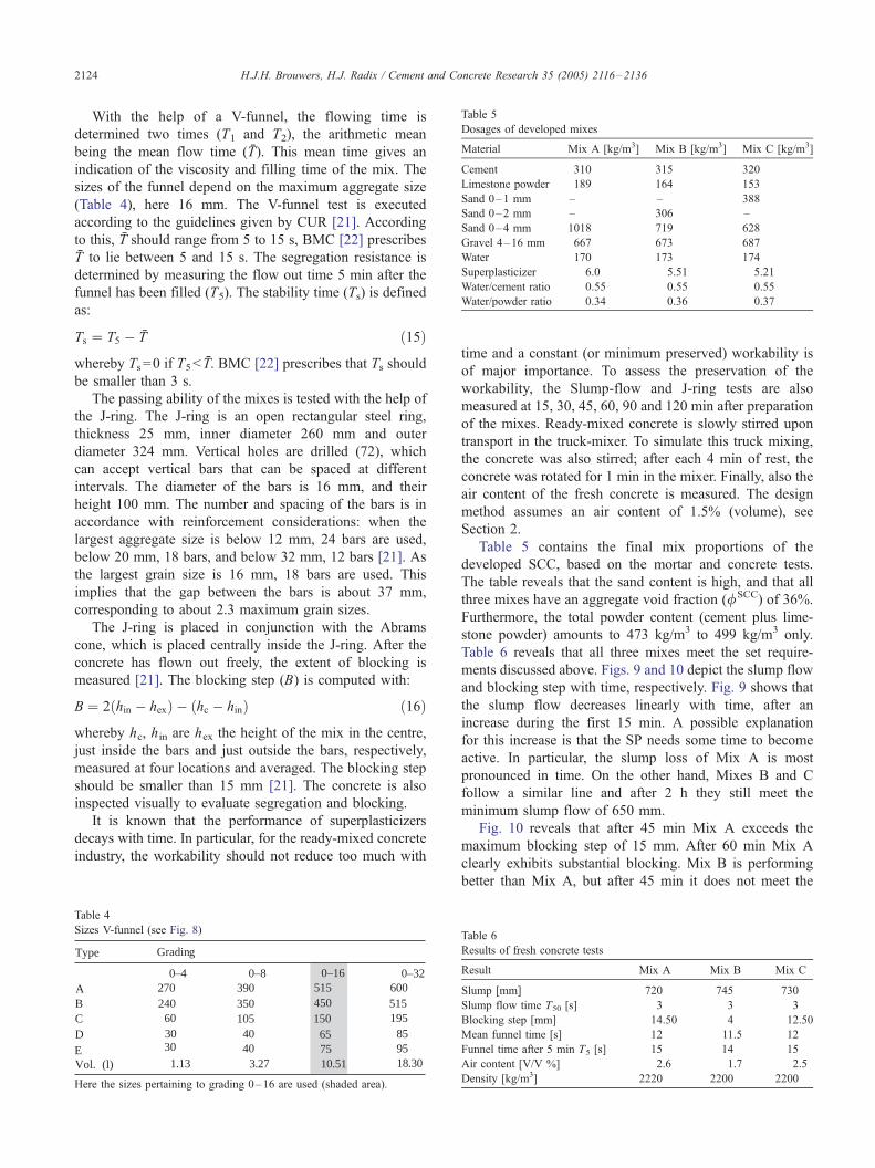
Table 5
Dosages of developed mixes
Material Mix A [kg/m3] Mix B [kg/m3] Mix C [kg/m3]
Cement 310 315 320
Limestone powder 189 164 153
Sand 0–1 mm – – 388
Sand 0–2 mm – 306 –
Sand 0–4 mm 1018 719 628
Gravel 4–16 mm 667 673 687
Water 170 173 174
Superplasticizer 6.0 5.51 5.21
Water/cement ratio 0.55 0.55 0.55
Water/powder ratio 0.34 0.36 0.37
H.J.H. Brouwers, H.J. Radix / Cement and Concrete Research 35 (2005) 2116–21362124
With the help of a V-funnel, the flowing time is
determined two times (T1 and T2), the arithmetic mean
being the mean flow time (T). This mean time gives an
indication of the viscosity and filling time of the mix. The
sizes of the funnel depend on the maximum aggregate size
(Table 4), here 16 mm. The V-funnel test is executed
according to the guidelines given by CUR [21]. According
to this, T should range from 5 to 15 s, BMC [22] prescribes
T to lie between 5 and 15 s. The segregation resistance is
determined by measuring the flow out time 5 min after the
funnel has been filled (T5). The stability time (Ts) is defined
as:
Ts ¼ T5 � T ð15Þ
whereby Ts=0 if T5< T. BMC [22] prescribes that Ts should
be smaller than 3 s.
The passing ability of the mixes is tested with the help of
the J-ring. The J-ring is an open rectangular steel ring,
thickness 25 mm, inner diameter 260 mm and outer
diameter 324 mm. Vertical holes are drilled (72), which
can accept vertical bars that can be spaced at different
intervals. The diameter of the bars is 16 mm, and their
height 100 mm. The number and spacing of the bars is in
accordance with reinforcement considerations: when the
largest aggregate size is below 12 mm, 24 bars are used,
below 20 mm, 18 bars, and below 32 mm, 12 bars [21]. As
the largest grain size is 16 mm, 18 bars are used. This
implies that the gap between the bars is about 37 mm,
corresponding to about 2.3 maximum grain sizes.
The J-ring is placed in conjunction with the Abrams
cone, which is placed centrally inside the J-ring. After the
concrete has flown out freely, the extent of blocking is
measured [21]. The blocking step (B) is computed with:
B ¼ 2 hin � hexð Þ � hc � hinð Þ ð16Þ
whereby hc, hin are hex the height of the mix in the centre,
just inside the bars and just outside the bars, respectively,
measured at four locations and averaged. The blocking step
should be smaller than 15 mm [21]. The concrete is also
inspected visually to evaluate segregation and blocking.
It is known that the performance of superplasticizers
decays with time. In particular, for the ready-mixed concrete
industry, the workability should not reduce too much with
Table 4
Sizes V-funnel (see Fig. 8)
Grading Type
0–4 0–8 0–32A 270 390 B 240 350 C 60 105 D 30 40 85
E 30 40 75Vol. (l)
600
9518.30
65
10.511.13 3.27
515
0–16515450150 195
Here the sizes pertaining to grading 0–16 are used (shaded area).
time and a constant (or minimum preserved) workability is
of major importance. To assess the preservation of the
workability, the Slump-flow and J-ring tests are also
measured at 15, 30, 45, 60, 90 and 120 min after preparation
of the mixes. Ready-mixed concrete is slowly stirred upon
transport in the truck-mixer. To simulate this truck mixing,
the concrete was also stirred; after each 4 min of rest, the
concrete was rotated for 1 min in the mixer. Finally, also the
air content of the fresh concrete is measured. The design
method assumes an air content of 1.5% (volume), see
Section 2.
Table 5 contains the final mix proportions of the
developed SCC, based on the mortar and concrete tests.
The table reveals that the sand content is high, and that all
three mixes have an aggregate void fraction (/SCC) of 36%.
Furthermore, the total powder content (cement plus lime-
stone powder) amounts to 473 kg/m3 to 499 kg/m3 only.
Table 6 reveals that all three mixes meet the set require-
ments discussed above. Figs. 9 and 10 depict the slump flow
and blocking step with time, respectively. Fig. 9 shows that
the slump flow decreases linearly with time, after an
increase during the first 15 min. A possible explanation
for this increase is that the SP needs some time to become
active. In particular, the slump loss of Mix A is most
pronounced in time. On the other hand, Mixes B and C
follow a similar line and after 2 h they still meet the
minimum slump flow of 650 mm.
Fig. 10 reveals that after 45 min Mix A exceeds the
maximum blocking step of 15 mm. After 60 min Mix A
clearly exhibits substantial blocking. Mix B is performing
better than Mix A, but after 45 min it does not meet the
Table 6
Results of fresh concrete tests
Result Mix A Mix B Mix C
Slump [mm] 720 745 730
Slump flow time T50 [s] 3 3 3
Blocking step [mm] 14.50 4 12.50
Mean funnel time [s] 12 11.5 12
Funnel time after 5 min T5 [s] 15 14 15
Air content [V/V %] 2.6 1.7 2.5
Density [kg/m3] 2220 2200 2200

640
650
660
670
680
690
700
710
720
730
740
750
0 20 40 60 80 100 120
Time after mixing [minutes]
Slu
mp
[mm
]
Mix A (sand 0-4 mm)
Mix B (sand 0-2 mm / 0-4 mm)
Mix C (sand 0-1 mm / 0-4 mm)
Minimum slump (CUR [21])
Fig. 9. Slump flow reduction with time.
H.J.H. Brouwers, H.J. Radix / Cement and Concrete Research 35 (2005) 2116–2136 2125
maximum allowable blocking step either. Mix C meets the
requirements during 60 min and exceeds the maximum
blocking step only slightly. It should be noted that the
blocking of Mixes B and C are very minor, only a slight
difference in height is noticeable across the J-ring. The
concrete still flows easily along the bars and does not
show any sign of segregation. Actually, a reading off error
from about 1 mm will already result in a blocking step that
is too large. The maximum value set by CUR [21] is quite
severe, and is only realistic when the mix height can be
measured with an accuracy of 0.1 mm (e.g. with laser).
That is the reason that in Germany the difference in
Slump-flow with and without J-ring is considered,
whereby the difference should be smaller than 50 mm
0
10
20
30
40
50
60
0 20 40 6
Time after mi
Blo
ckin
g st
ep B
[mm
]
Fig. 10. Blocking step in
[23]. This difference is easier to measure, and all three
mixes meet this requirement. The high retention of filling
and passing abilities is most probably owed to the type of
plasticizer used. Hanehara and Yamada [24] also observed
a longer workability when using a polycarboxylate type
admixture.
Table 6 also contains the measured air content and
density of the concrete. The air content is higher than 1.5%
as assumed during the mix computations. As possible
explanation is that the concrete did not have enough time
to de-air (5 min) after filling the air-pressure container. But
all values are well within the maximum air content of 3%
(NEN 5962 [25]). The densities of all three mixes are
close. Mix A possesses a slightly higher density as it
0 80 100 120
xing [minutes]
Mix A (sand 0-4 mm) Mix B (sand 0-2 mm / 0-4 mm) Mix C (sand 0-1 mm / 0-4 mm) Maximum B (CUR [21])
crease with time.

0.1
1
10
100
0.1 1 10 100 1000 10000 100000
Particle size (D) [µm]
% C
umul
ativ
e fin
er (
V/V
)
Mix AMix BMix CModified A&A model (eq. (14)), Dmax = 16 mm, Dmin = 0.5 µm, q = 0.25A&A model (eq. (13)), Dmax = 16 mm, q = 0.25Fuller model (eq. (13)), Dmax = 16 mm, q = 0.5
Fig. 11. Cumulative finer mass fraction of Mixes A, B and C in double-logarithmic graph.
H.J.H. Brouwers, H.J. Radix / Cement and Concrete Research 35 (2005) 2116–21362126
contains more powder (Table 5). Mixes B and C have the
same density, although Mix C contains less powder than
Mix B. But Mix C contains 5 kg/m3 cement more, which
has a higher specific density than all other constituents
(Tables 1, 5 and 6).
6. Grading
In Figs. 11 and 12 the PSD (cumulative finer) of the three
mixes are given comprising all solids. In the single-
logarithmic graph the grading of the coarse material can
be read off clearly. By presenting the PSD also in a double-
logarithmic graph, possible deviations in the grading of the
0
10
20
30
40
50
60
70
80
90
100
0.1 1 10 10
Particle size
% C
umul
ativ
e fin
er (
V/V
)
Mix A
Mix B
Mix C
A&A model (eq. (13)), Dmax = 16 mm, q = 0.25
Modified A&A model (eq. (14)), Dmax = 16 mm, Dmin
Fuller model (eq. (13)), Dmax = 16 mm, q = 0.5
Fig. 12. Cumulative finer mass fraction of Mixe
fine material (<250 Am) become clear. In both figures also
the curves following the A&A grading, the modified A&A
grading and the Fuller grading are included.
Figs. 11 and 12 readily reveal that the PSD of the three
mixes does not follow the Fuller curve, which is used for
‘‘normal’’ concrete. The designed three mixes follow as
much as possible the PSD from the modified A&A grading
(with q =0.25), as recommended by [11]. However, the
PSD from the three mixes cannot follow the modified
A&A curve perfectly, as the PSDs of the constituents used
are S-shaped (Fig. 2). Especially, between 100 Am and 4
mm one can see a disturbance, which can be explained by
the fact that in this particle range the sand contributes
significantly to the PSD. The S-shaped pattern corresponds
0 1000 10000 100000
(D) [µm]
= 0.5 µm, q = 0.25
s A, B and C in single-logarithmic graph.

H.J.H. Brouwers, H.J. Radix / Cement and Concrete Research 35 (2005) 2116–2136 2127
to the pattern of the sand (Fig. 2). In order to avoid this
deviation, more constituents with overlap in their particle
sizes should be used. One can think on the application of
sand 2–4 mm and gravel 4–8 mm.
It is expected that a grading that more closely follows the
modified A&A curve will result in a mix with a better
workability and stability. The three concrete mixes revealed
that indeed Mix C exhibited a better resistance to
segregation and workability. The required amount of SP in
this mix is also lower than in the two other mixes, whereas
their slump flows and funnel times are almost equal. The
addition of fine sand (0–1 mm) has improved the flowing
properties of the mix, so that the amount of powders and SP
can be reduced.
Using the modified A&A grading curve, the part of
fine materials (<250 Am) is about three times higher than
with the application of the Fuller curve. Table 7 lists the
amount of fine materials in the three mixes. Table 7
shows that Mix C contains much more fine material than
Mixes A and B, and that the quantity of the stone powder
is least in Mix C. Hence, by application of fine sand (0–
1 mm) it is possible to increase the amount of fine
materials, while at the same time reducing the quantity of
cement and filler. The volume of fine material in Mix C
amounts to about 0.245 m3 per m3 of concrete, which is
about two times the minimum amount prescribed by NEN
5950 [14] for concrete with a maximum particle size of
16 mm (Table 2b). This reduction of powders and
superplasticizer in case of fine sand application can also
be explained by comparing the PSDs of the three mixes.
The PSD of Mix C follows best the modified A&A
curve, especially between 100 Am and 1 mm (Figs. 11
and 12).
Considering Tables 1 and 5, it follows that all solids
(cement, limestone powder and aggregate) take about 81%
of the volume of all mixes, i.e. the void fraction amounts
about 19%. It is interesting to compare this value with the
Table 7
Amount of fine material (<250 Am) per m3 of concrete
Mix A Mix B Mix C
Volume fraction fine
material (<250 Am)
0.195 0.189 0.245
Mass of cement [kg/m3] 310 315 320
Mass of stone powder
[kg/m3]
189 164 153
Part of sand 0–1 mm
smaller than 250 Am[kg/m3]
– – 180
Part of sand 0–2 mm
smaller than 250 Am[kg/m3]
– 20 –
Part of sand 0–4 mm
smaller than 250 Am[kg/m3]
55 39 34
Total mass of fine material
(D <250 Am) [kg/m3]
554 538 687
void fraction of an ideal mix that obeys Eq. (14), which
reads [26]:
u ¼ u1
Dmin
Dmax
� � 1�u1ð Þb1þq2ð Þ
ð17Þ
This equation contains the void fraction of the single-
sized particles (u1) and a parameter (b), which are both
governed by the particle shape and method of packing
(loose, close) only. From [9,26] it follows that for the
irregular particles considered here, u1=0.52 and b =0.16
(loose), and u1=0.46 and b =0.39 (close). Furthermore,
substituting Dmin=0.5 Am, Dmax=16 mm and q=0.25,
yields u =25% and u =6% for loose and close random
packing, respectively. Hence, the void fraction of Mixes A,
B and C (19%) are situated between these aforementioned
two extremes.
The concrete mix tests yield the conclusion that the PSDs
and the content of fine materials (<250 Am) greatly
influence the stability and workability of the mix. The
application of fine sand helps to optimise both content and
PSD in the fine particle range, so that the amount of
required SP can be reduced. This application of fine sand
also reduces the ingredient costs of the mix. Fine sand is
relatively cheap; it is cheaper than the two other sands and
than gravel, and replaces the most expensive constituents:
cement and stone powder (the powders). Furthermore,
composing a mix with a PSD that closely follows the
modified A&A model reduces another expensive ingredient,
namely the SP. It could be expected that if one would
optimise the PSD down in the nanometre range, the
workability and stability could be maintained while further
reducing the necessary SP content. In the next section the
tests on the hardened concrete are reported.
7. Hardened concrete experiments
The three mixes have been poured in standard cubes of
150�150�150 mm3, cured sealed during the first day,
demoulded, and subsequently cured for 27 days submersed
in a water basin. In total, 138 cubes have been produced
which are tested physically and mechanically. Of each mix,
46 cubes have been produced, 44 for testing, and 2 as
reserve. Since the concrete mixer in the laboratory has a
limited capacity (25 l), each mix is made in 7 batches: 6
batches of 25 l and 1 batch of 20 l, yielding a total of 170 l
for each mix.
The density of the hardened concrete is determined by
measuring the weight of a cube in the air and underwater,
according to standard NEN 5967 [27]. The density is
computed by
qcube ¼ qw
M aircube
M aircube �Mwater
cube
ð18Þ

Table 8
Apparent density of hardened concrete
Mix A Mix B Mix C
Mean cube density [kg/m3] 2370 2360 2350
Standard deviation [kg/m3] 33.3 13.0 7.5
Coefficient of variation [%] 1.4 0.6 0.3
Table 9
Compressive strength (in N/mm2) after 1 day (a), 3 days (b), 7 days (c) and
28 days (d) curing
Mix A Mix B Mix C
a)
Mean compressive strength [N/mm2] 5.7 3.9 5.9
Standard deviation [N/mm2] 0.1 0.7 0.1
Coefficient of variation [%] 1.8 17.9 1.7
b)
Mean compressive strength [N/mm2] 17.2 16.9 18.4
Standard deviation [N/mm2] 0.3 0.6 0.2
Coefficient of variation [%] 1.7 3.6 1.1
c)
Mean compressive strength [N/mm2] 31.2 28.3 34.0
Standard deviation [N/mm2] 1.8 0.8 1.0
Coefficient of variation [%] 5.8 2.8 2.9
d)
Mean compressive strength [N/mm2] 51.2 50.7 53.6
Standard deviation [N/mm2] 1.5 1.7 1.8
Coefficient of variation [%] 2.9 3.4 3.4
Characteristic compressive strength [N/mm2] 47.6 46.7 49.3
x [N/mm2 per kg cement/m3 concrete] 0.154 0.148 0.154
H.J.H. Brouwers, H.J. Radix / Cement and Concrete Research 35 (2005) 2116–21362128
where Maircube and Mwater
cube are the weights of the concrete
cube in air and water, respectively. The mean values of all
cubes are listed in Table 8. In this table also the two
statistical parameters, standard deviation (s) and variation
coefficient (VC), are given. The standard deviation is
computed with:
s ¼
ffiffiffiffiffiffiffiffiffiffiffiffiffiffiffiffiffiffiffiffiffi~ yi � yð Þ2
m� 1
sð19Þ
where yi is each measured value, y their arithmetic mean
value, and m the number of measured values. The
coefficient of variation is computed by
CV ¼ s
yð20Þ
The s and CV listed in Table 8 show that all batches have
resulted in concrete with almost constant density (the
difference is less than 1%), so that all batches are very
homogeneous and identical.
The compressive strength ( fc) of each cube is
measured according to standard NEN 5968 [28]. At ages
of 1, 3, 7 and 28 days, 5 cubes per mix are tested and the
resulting mean values are listed in Table 9a–d and
depicted in Fig. 13a.
Mix C has the highest compressive strength; application
of the fine sand (0–1 mm) seems to contribute to the
strength, most likely by a better packing of the particles.
Though Mix B contains medium sand (0–2 mm) and more
cement than Mix A, it has a lower compressive strength than
Mix A.
To classify the mixes, the characteristic compressive
strength ( f Vck), being the strength that is statistically attained
by 95% of the material, is determined. It follows from the
mean value (y), the standard deviation (s) and the
eccentricity ratio (e) as:
fckV V y� eIs ð21Þ
The value of e depends on the number of tested cubes
(here: 5). In Table 10 the values of e are listed assuming a
normal (Gaussian) distribution, here e=2.37. In Table 9d
the characteristic 28 days strength is included, indicating
that the three mixes can be classified as C35/45 (former
B45).
In Section 3 it was discussed that Su et al. [6] and Su
and Miao [7] used a parameter x to describe the strength
of concrete as a function of the cement content (Eq. (4)).
To assess the value of x for the cement used here, the
characteristic compressive strength (Table 9d) is divided
by the cement content of the mix (Table 5) and included
in Table 9d. The values found for slag cement CEM III/
B 42.5 N LH/HS used here, around 0.15 N/mm2, are
higher than the values of Type I Portland Cement, 0.11
to 0.14 N/mm2, reported by Su et al. [6] and Su and
Miao [7].
Next, the tensile strength is measured using the indirect
splitting test, according to standard NEN 5969 [29]. Two
plywood strips (thickness 3 mm, width 15 mm and length
160 mm) are used as bearing strips. At ages of 1, 3, 7 and 28
days, 5 cubes per mix are tested, and the resulting mean
values are listed in Table 11a–d and depicted in Fig. 13b.
The tensile strength follows from:
ft ¼2F
pz2ð22Þ
where F is the applied yield force and z the side of the
cube (z=150 mm). Likewise the compressive strength
(Table 9a–d), Mix C also has the highest tensile strength.
The tensile strength is related to the compressive strength.
For ‘‘normal concrete’’ the 28 days (splitting) tensile
strength ( ft) can be computed from the compressive
strength ( fc) by NEN 6722 [30] as:
ft ¼ 1 N=mm2 þ 0:05fc ð23Þ
The measured tensile and compressive strengths of the 3
mixes are depicted in Fig. 14, at an age of 28 days. In
this figure also Eq. (23) is included. The experimental

0
5
10
15
20
25
30
35
40
45
50
55
0 5 10 15 20 25 30
Age [days]
Com
pres
sive
str
engt
h [N
/mm
2 ]
Mix AMix BMix C
a)
0
0.5
1
1.5
2
2.5
3
3.5
4
4.5
5
0 5 10 15 20 25 30
Age [days]
Ten
sile
str
engt
h [N
/mm
2 ]
Mix AMix BMix C
b)
Fig. 13. a) Compressive strength versus age. b) Tensile strength versus age.
H.J.H. Brouwers, H.J. Radix / Cement and Concrete Research 35 (2005) 2116–2136 2129
results show that the SCC mixes perform better than the
empirical correlation (Eq. (23)). This is in line with CUR
[21], where it was concluded that the tensile strength of
SCC is systematically higher than that of ‘‘normal
concrete’’.
Subsequently, the durability of the mixes is inves-
tigated by measuring the intrusion of water, by absorp-
Table 10
Eccentricity factor versus number of tests
Number of
specimen
12 11 10 9 8 7 6 5 4 3 2
Eccentricity
factor
1.53 1.60 1.68 1.77 1.87 2.00 2.16 2.37 2.65 3.06 3.75
tion and by pressure at an age of 28 days. The intrusion
of water is measured by exposing one face of the cube
to water pressure of 5 bars (0.5 MPa), according to
standard NEN-EN 12390-8 [31]. After 72 h the cubes
are removed from the test rig, and split perpendicularly
with respect to the tested face following NEN 5969
[29]. The location of the waterfront, at both halves,
can be observed visually and the distance from the
cube side measured (Fig. 15). For each mix, two cubes
are tested accordingly. In Table 12 the results are
listed.
The results indicate that the addition of fine sand (0–1
mm) and medium sand (0–2 mm) have a beneficial effect
on water resistance. Mix B is having slightly less water
intrusion that Mix A, but Mix C clearly has a much lower

Waterfront
Fig. 15. Photo of water intrusion in one half of the cube.
Table 11
Tensile strength (in N/mm2) after 1 day (a), 3 days (b), 7 days (c) and 28
days (d) curing
Mix A Mix B Mix C
a)
Mean tensile strength [N/mm2] 0.6 0.4 0.7
Standard deviation [N/mm2] 0.02 0.12 0.01
Coefficient of variation [%] 3.3 30.0 1.4
b)
Mean tensile strength [N/mm2] 1.9 1.7 2.0
Standard deviation [N/mm2] 0.09 0.14 0.08
Coefficient of variation [%] 4.7 8.2 4.0
c)
Mean tensile strength [N/mm2] 2.9 2.9 3.3
Standard deviation [N/mm2] 0.14 0.10 0.16
Coefficient of variation [%] 4.8 3.4 4.8
d)
Mean tensile strength [N/mm2] 4.2 4.1 4.7
Standard deviation [N/mm2] 0.27 0.27 0.20
Coefficient of variation [%] 6.4 6.6 4.3
H.J.H. Brouwers, H.J. Radix / Cement and Concrete Research 35 (2005) 2116–21362130
permeability than both other mixes. Concrete with less than
50 mm intrusion is regarded as impermeable [23]. All three
mixes meet this requirement and can be classified as
impermeable.
Next, the capillary absorption is measured, analogous to
Audenaert et al. [32] and Zhu and Bartos [33]. Prior to the
experiment, the cubes (of age 28 days) were dried in an
oven at 105T5 -C during 48 h, and cooled down during
24 h at room temperature. Then, the cubes were placed on
bars with a diameter of 10 mm, so that the water level is
5T1 mm above the lower horizontal face of the cube. For
each mix, two cubes have been tested. The mass increase
of each cube is measured after 0.25, 0.5, 1, 3, 6, 24, 72
0
1
2
3
4
5
6
0 10 20 30 40
Compressive s
Ten
sile
str
engt
h [N
/mm
2 ]
Mix A
Mix B
Mix C
Relation in NEN 6722 [30] (eq.(23))
Fig. 14. Tensile strength versus com
and 168 h (Fig. 16). Furthermore, the height of the
capillary rise is measured on the 4 vertical side faces (in
the centre of the side) of each cube; the mean values of
each cube, H, are given in Fig. 17.
There is a linear relation between the capillary rise and
the square root of time [32,33]:
H ¼ H0 þ SIT 0:5 ð24Þ
In this equation is H the height of the capillary rise, H0
the intersection with the y-axis [mm], SI the sorption
index [mm/h0.5] and T the time (h). The SI is a measure
for the uptake of water by a concrete surface exposed to
50 60 70 80 90
trength [N/mm2]
pressive strength (28 days).

Table 12
Water intrusion and permeability (28 days)
Specimen Intrusion depth [mm]
Side 1 Side 2 Mean
Mix A, cube 1 30 26 28
Mix A, cube 2 30 24 27
Mix B, cube 1 17 21 19
Mix B, cube 2 21 26 23.5
Mix C, cube 1 8 6 7
Mix C, cube 2 10 7 8.5
H.J.H. Brouwers, H.J. Radix / Cement and Concrete Research 35 (2005) 2116–2136 2131
rain for instance. In Audenaert et al. [32] it can be found
that SI should be smaller than 3 mm/h0.5. Using linear
regression, the SI is derived from the data in Fig. 17, and
listed in Table 13, including the regression coefficient of
the fit. One can see that now Mix C is having the highest
value, indicating that the fine sand is favourable for
capillary suction. But Table 13 also reveals that all mixes
have an SI that is well below 3 mm/h0.5, so that this
durability criterion is met.
8. Analysis of powder (paste) and aggregate (vibration)
experiments
In this section the aggregate compaction and paste
flow spread tests from Section 2 will be analysed in
detail. A relation will be derived between the amount
of water that can be retained and the void fraction of
the powder. Furthermore, a relation will be derived
between the slope of the paste line, and the internal
specific surface area of the powder. Based on both
powder and aggregate data, a general relation is derived
that describes the reduction in void fraction upon
compaction.
0
20
40
60
80
100
120
0 42 6
Time
Mas
s in
crea
se o
f cub
e [g
]
Mix A, cube 1Mix A, cube 2Mix B, cube 1Mix B, cube 2Mix C, cube 1Mix C, cube 2
Fig. 16. Mass increase of concrete cub
Fig. 5 shows the relative slump, a measure for the
flowability, and the ratio of water and powder volume.
To interpret this data, two hypotheses will be put
forward and validated. First, when sufficient water is
present for flow, so Vw/Vp>bp, the relative slump
depends on the specific surface area of the powder.
This is motivated by the concept that water in surplus of
Vpbp is able to lubricate the particles. The thickness of
this water film, which governs flowability and slump,
depends on the internal specific surface area of the paste.
Second, it is assumed that the paste will flow when
Cp>0, so there is sufficient water to fill the voids of the
powder.
The fitted paste lines of the powders: cement, fly ash and
stone powder in Fig. 5, are of the form:
Vw ¼ apCp þ bp
� �Vp ð25Þ
The fitted coefficients ap and bp are listed in Table 14. To
verify the first hypotheses, the deformation coefficient ap is
divided by specific surface area S, i.e. the Blaine surface per
volume of powder. The specific surface areas of the three
powders are listed in Tables 1 and 14, and follow from
Blaine multiplied by the particle density. From the limited
amount of data, one might draw the conclusion that the
larger the internal surface, the larger the deformation
coefficient (the more water is required to attain a certain
relative slump, see Fig. 5). Accordingly, a linear relation is
invoked:
ap ¼ dIBlaineIqp ¼ dIS ð26Þ
Substituting ap and S from the three powders yields
that d ranges from 3.570�10�6 cm to 4.478�10�6 cm
8 10 12 14
[hour0.5]
e by capillary suction with time.

0
5
10
15
20
25
30
35
40
45
50
55
0 2 4 6 8 10 12 14
Time [hour0.5]
Hei
ght c
apill
ary
rise
[mm
]
Mix A, cube 1 Mix A, cube 2 Mix B, cube 1 Mix B, cube 2 Mix C, cube 1Mix C, cube 2
Fig. 17. Mean capillary rise of each cube with time.
H.J.H. Brouwers, H.J. Radix / Cement and Concrete Research 35 (2005) 2116–21362132
(Table 14), with d =4.132�10�6 cm being a mean
value that matches all three computed values of y(within 13.6%). In Fig. 18a the experimental ap and S
and Eq. (26) with d =41.32 nm are set out. Further-
more, comparable data taken from Domone and Wen
[13] are included in Table 14 and Fig. 18a, which can
also be described adequately with Eq. (26) and
d =4.132�10�6 cm.
Subsequently, the second hypothesis is considered.
From the paste lines it is assumed that if Vw=Vpbp, the
voids will be completely filled with water, in other
words:
/dp ¼
Vw
Vw þ Vp
¼bp
bp þ 1ð27Þ
In Table 14, this computed void fraction is included. In
Table 14 also the ratio of this void content and the void
content in loose state is included. This loosely packed
void fraction, /p1, of the powders are computed with Eq.
(2) and using the powder properties listed in Table 1. For
Table 13
Regression results of height capillary rise
Specimen Intersection y-axis
(H0) [mm]
Sorption index
(SI) [mm/h0.5]
R2
Mix A, cube 1 20.57 1.63 0.977
Mix A, cube 2 21.99 1.03 0.951
Mix B, cube 1 20.69 1.54 0.988
Mix B, cube 2 22.07 2.11 0.994
Mix C, cube 1 20.43 1.82 0.962
Mix C, cube 2 20.39 1.89 0.985
all the powders, it seems that there is constant ratio
between both void contents, hence:
/dp ¼ 0:77/1
p ð28Þ
Apparently, the voids to be filled with water (following from
Eq. (27), i.e. from the paste line) are less than present in the
same powder when it loosely piled, but there is a constant
ratio between them. Upon mixing of the powder with water
some compaction will take place, this is the reason this void
fraction is assigned with the superscript ‘‘d’’ in Eqs. (27) and
(28). It seems that this mixing with water results in a void
reduction of about for all powders 23%. Upon vibrating the
aggregates, in Section 2 the reduction in void fraction was
practically the same. Accordingly, in Fig. 18b the loosely
piled void fraction and the compacted void fraction of the
three sands and of the gravel, and of the 50% mixes of the
three sands and the gravel, taken from Fig. 3, are set out.
Furthermore, for the three powders, the void fraction from
the loosely piled powder (Table 14) and the void fraction
obtained with the paste lines (Eq. (27)) are also included in
this figure. Eq. (28), included in this figure as well, matches
all values with a good accuracy. Besides these irregularly
shaped powders and aggregates, Eq. (28) seems to approach
the ratio for spheres as well. For random close packing of
uniform spheres, /pd=0.36 prevails [34,35], whereas for
random loose packing of spheres in the limit of zero gravity,
/p1=0.45 prevails [36].
Now, from the present analysis, one can assess bp as
follows:
bp ¼/dp
1� /dp
¼qp � qd
p
qdp
¼0:77/d
p
1� 0:77/dp
¼0:77 qp � q1
p
� �q1p þ 0:23qp
ð29Þ

Table 14
Analysis of powders and paste lines (* taken from Domone and Wen [13])
Material Sp [cm2/cm3] /l
p ap d [cm] bp /pd /p
d//pl
CEM III/B 42.5 N LH/HS 13,865 0.63 0.062 4.46�10�6 0.97 0.49 0.78
Fly ash 8775 0.56 0.039 4.48�10�6 0.78 0.44 0.79
Limestone powder 12,604 0.60 0.045 3.57�10�6 0.82 0.45 0.75
Portland cement* 11,844 – 0.061 5.15�10�6 1.08 0.52 –
GGBS* 12,180 – 0.046 3.77�10�6 1.10 0.52 –
H.J.H. Brouwers, H.J. Radix / Cement and Concrete Research 35 (2005) 2116–2136 2133
see Eq. (2). Eqs. (26) and (29) enable the computation of ap
and bp for a given powder using its Blaine surface, the
particle density and the loosely piled density (or, instead of
the latter, the density in compacted state). Domone and Wen
0
0.01
0.02
0.03
0.04
0.05
0.06
0.07
0 2000 4000 6000 8
Blaine * ρ
αp
Experimental
Literature (Domone and Wen [13])
a)
0
0.1
0.2
0.3
0.4
0.5
0.6
0 0.1 0.2 0.3
Loose app
Den
se a
ppar
ent d
ensi
ty
Powder
Aggregate
eq. (28)
b)
Fig. 18. a) Relation between deformation coefficient from the paste lines and the sp
b) Relation between water retention capacity of three powders (from paste lines, F
the four aggregates the loosely state and compacted state void fractions are also inc
on data from Fig. 3).
[13] demonstrated that these parameters, in turn, are directly
related to yield stress and plastic viscosity of the paste.
Note that ap and bp are the parameters in the volume
paste line (Eq. (25)). The Chinese Method makes use of
000 10000 12000 14000 16000
p (cm2/cm3)
y = 4.13E-06x R2 = 0.96
0.4 0.5 0.6 0.7 0.8
arent density
ecific surface of the powder per unit of volume. Data is taken from Table 14.
ig. 6 and Table 14) and the void fraction of the loosely piled powders. From
luded, as well as of the 50% mixes of the three sands with the gravel (based

H.J.H. Brouwers, H.J. Radix / Cement and Concrete Research 35 (2005) 2116–21362134
Eqs. (6), (10), (11) and (12), which contain the parameters
of the mass paste lines. They are related by:
ap ¼qwapqp
; bp ¼qwbp
qp
ð30Þ
Here, basic relations have been derived for powder–water
mixes tested with the Haegermann cone. It is expected that
similar basic relations could be derived for concrete mixes
and Abrams cone that relate the parameters of slump lines at
one hand, with the specific surface area per volume of solid
constituents in the mix and their loosely/packed densities at
the other hand.
9. Conclusions
The Japanese Method makes use of the packed densities
of gravel and sand individually, in the Chinese Method the
packing of these aggregates is considered integrally. In this
study the packing of all solids in the mix (gravel, sand, filler
and cement) is considered, which was actually recommen-
ded already by Fuller and Thompson ([15], pp. 242–244).
Ideally, the grading curve of all solids should follow the
modified Andreasen and Andersen curve. Indeed, it
followed that the aggregates used by Su et al. [6] and Su
and Miao [7] followed this curve (Eq. (13), q =0.30).
Furthermore, combining the solids, the quantity of paste
(water, cement and filler) should be reduced as much as
possible. In this paper, it is analysed which combinations of
three sands, gravel, SP and slag blended cement result in the
lowest powder (cement, limestone powder) content.
Based on these considerations, three mixes have been
composed and tested (Table 5) that obey q =0.25 as much
as possible. Another objective was to meet these theoret-
ical requirements while using the most economical
ingredients. This has resulted in three mixes with a low
content of powder, T480 kg/m3 of concrete. The fresh
concrete has been evaluated with the Slump-flow, V-funnel
and J-ring tests, and its air content has been measured. All
mixes meet the criteria set by these tests, whereby the use
of superplasticizer could be limited to 1% of the powder
content, and the use of a viscosity modifying agent can be
avoided.
Up to an age of 28 days, the cured concrete has been
tested physically (density, water absorption, etc.) and
mechanically (compressive and splitting tensile strengths).
The compressive strength tests reveal that the three mixes
result in concretes that can be classified as C35/45. The
objective of composing medium strength concrete is there-
fore achieved. It also follows that for the slag cement used
(CEM III/B 42.5 N LH/HS), the compressive strength/
cement content ratio (x) amounts to 0.15 N/mm2 per kg
cement/m3 concrete. This measure for the cement efficiency
lies within the same range as the values reported by Su et al.
[6] and Su and Miao [7]: 0.11–0.14 N/mm2 per kg cement/
m3 concrete for Type I Portland Cement. The tensile
strength, obtained with the splitting test, appears to be
higher than ‘‘normal concrete’’ of comparable compressive
strength.
The hardened concrete mixes are also tested on their
durability, using both the water intrusion and capillary
suction test. Both tests yield that all three mixes can be
classified as impermeable and durable. So, using the
packing theory of Andreasen and Andersen [9], and its
modifications by Funk and Dinger [10] and Elkem [11],
cheap SCC mixes can be composed that meet the standards
and requirements in fresh and hardened states. Furthermore,
a carboxylic polymer type superplasticizer is employed as
sole admixture; an auxiliary viscosity enhancing admixture
is not needed to obtain the required properties.
Finally, the paste lines are examined and general relations
derived. For future application of other powders these
relations permit an assessment of the parameters ap and bpof the powder (Eqs. (26), (29) and (30)), which in turn can
be used to compose the SCC mix (Eqs. (6), (10), (11) and
(12)), without the need of cumbersome flow spread tests of
the paste. It furthermore follows that the void fraction of
both aggregates and powders used are reduced by about
23% upon compaction. This similarity in compaction
behaviour could be attributed to the similar (S-) shape
PSD of all materials used (Fig. 2).
List of Symbols
Roman
ap deformation coefficient
bp retained water ratio
B blocking step [m]
c mass of cement [g]
CV coefficient of variation
d slump [m]
dm dry matter
D particle size [m]
Dmin minimum particle size [m]
Dmax maximum particle size [m]
e eccentricity ratio
fc compressive strength [N/mm2]
f Vck characteristic compressive strength [N/mm2]
ft tensile strength [N/mm2]
F force [N]
h mix height [m]
H height capillary rise [m]
H0 height capillary rise at T=0 [m]
M mass [kg]
m number of specimen
n mass of SP per mass of powder (cement plus filler)
P cumulative finer fraction
PF packing factor
q parameter in (modified) Andreasen and Andersen
model

H.J.H. Brouwers, H.J. Radix / Cement and Concrete Research 35 (2005) 2116–2136 2135
PSD particle size distribution
RH relative humidity
s standard deviation
S specific surface area per unit of volume [cm2/cm3]
SI sorption index [mm/h0.5]
SP superplasticizer
T time [s]
T5 V-funnel flow out after 5 min [s]
T50 time at which the concrete reaches the 50 cm circle
[s]
Ts stability time (Eq. (15)) [s]
V volume [m3]
x compressive strength per kg cement/m3 concrete
[Nm3/kgmm2]
z the side of a cube [m]
Greek
ap deformation coefficient
bp retained water ratio
b parameter (Eq. (17))
d parameter [cm]
u void fraction
q density [g/cm3]
C relative slump
Subscript
a aggregate
air air
c cement
cube cube
f filler (fly ash, stone powder)
m mortar
p powder (cement, filler)
tot total
w water
Superscript
air in air
d densely packed
water underwater
l loosely packed
SCC Self-Compacting Concrete
/ mean
Acknowledgements
The authors would like to express their gratitude to Mrs.
Ir. W.J. Bouwmeester-Van den Bos, Ing. H. ter Welle, Mr. B.
Bos and Mr. B. Piscaer for their advice. They furthermore
would like to thank their colleagues Ing. G.H. Snellink and
Mr. H.M. Menkehorst for the laboratory support. The
authors furthermore wish to thank the following institutions
for their financial support of the Cement-Concrete-Immo-
bilisates Research: Cornelis Lely Foundation, Delta Marine
Consultants, Betoncentrale Twenthe, Rokramix, Dutch
Ministry of Infrastructure, Senter Novem Soil, Jaartsveld
Groen en Milieu.
References
[1] H. Okamura, Self-compacting High-Performance Concrete, Concrete
International 19 (7) (1997) 50–54.
[2] H. Okamura, M. Ouchi, Self-Compacting Concrete—development,
present, and future, RILEM, Proc. 1st International RILEM Sympo-
sium on Self-Compacting Concrete, 1999, pp. 3–14.
[3] H. Ter Welle, Betoncentrale Twenthe, Hengelo, The Netherlands,
Personal communications (2003).
[4] B. Bos, BAS, Venray, The Netherlands, Personal communications
(2003).
[5] F.M.L. Ernst, Onderzoek zelfverdichtend beton. MSc Thesis
TUE/CCO/00-09, Eindhoven University of Technology, Faculteit
Bouwkunde, Capaciteitsgroep Constructief Ontwerpen, Eindhoven,
The Netherlands, 2000 (in Dutch).
[6] N. Su, K.C. Hsu, H.W. Chai, A simple mix design method for Self-
Compacting Concrete, Cement and Concrete Research 31 (2001)
1799–1807.
[7] N. Su, B. Miao, A new method for mix design of medium strength
concrete with low cement content, Cement & Concrete Composites 25
(2003) 215–222.
[8] A.M. Neville, Properties of Concrete, 4th edR, Prentice Hall/Pearson,
Harlow, 2000.
[9] A.H.M. Andreasen, J. Andersen, Ueber die Beziehung zwischen
Kornabstufung und Zwischenraum in Produkten aus losen Kornern
(mit einigen Experimenten), Kolloid-Zeitschrift 50 (1930) 217–228
(in German).
[10] J.E. Funk, D.R. Dinger, Predictive Process Control of Crowded
Particulate Suspension, Applied to Ceramic Manufacturing, Kluwer
Academic Press, 1994.
[11] Elkem Materials, User Documentation Language Independent Size
Distribution Analyser (L.I.S.A), http://www.refractories.elkem.com
(2003).
[12] H.J. Radix, Chinese mengselontwerpmethode voor Zelfverdichtend
Beton; Onderzoek naar goedkope ZVB mengsels met normale
druksterkte, op basis van een nieuwe ontwerpmethode en de
toepassing van fijn zand. MSc thesis, University of Twente,
Faculty of Engineering Technology, The Netherlands, 2004 (in
Dutch).
[13] P. Domone, C.H. Wen, Testing of binders for High Performance
Concrete, Cement and Concrete Research 27 (1997) 1141–1147.
[14] Dutch Normalization-Institute, NEN 5950:1995 Voorschriften Beton
Technologie. Eisen, vervaardiging en keuring, Nederlands Normal-
isatie Instituut, Delft, The Netherlands, 1995, (in Dutch).
[15] W.B. Fuller, S.E. Thompson, The laws of proportioning concrete,
Transactions of the American Society of Civil Engineers 33 (1907)
222–298.
[16] A.M. Gaudin, An investigation of crushing phenomena, Petroleum
Development and Technology 73 (1926) 253–316.
[17] BFBN, Cursushandboek Zelfverdichtend Beton, Bond van Fabri-
kanten van Betonproducten in Nederland (BFBN), Woerden, The
Netherlands, 2001, (in Dutch).
[18] EFNARC, Specification and Guidelines for Self-Compacting Con-
crete. EFNARC (European Federation of Producers and Applicators
of Specialist Products for Structures), 2002 (February). http://www.
efnarc.org/pdf/SandGforSCC.PDF.
[19] S.F.A. Ankone, Zelfverdichtend Beton. Training Period Report,
University of Twente, Faculty of Engineering Technology, The
Netherlands, 2000, (in Dutch).
[20] J.C. Walraven, K. Takada, G.I. Pelova, Zelfverdichtend beton, hoe
maak je dat?, Cement (The Netherlands) 3 (1999) 68–72 (in
Dutch).

H.J.H. Brouwers, H.J. Radix / Cement and Concrete Research 35 (2005) 2116–21362136
[21] CUR, CUR-Aanbeveling 93, Zelfverdichtend Beton, Stichting CUR,
Gouda, The Netherlands, 2002, (in Dutch).
[22] BMC, Aanvulling BRL 1801, Aanvulling op de Nationale
Beoordelingsrichtlijn Betonmortel (BRL 1801), Hoogvloeibare,
verdichtingsarme en zelfverdichtende betonmortel. Certificatie
Instelling Stichting BMC, Gouda, The Netherlands, 2002.
http://www.bmc-cert.nl/nederlands/brl/1801_aanvulling_zvb.pdf (in
Dutch).
[23] H.W. Reinhardt, DAfStb guideline on self compacting concrete, BFT
(Beton+Fertigteil�Technik) 67 (12) (2001) 54–62.
[24] S. Hanehara, K. Yamada, Interaction between cement and chemical
admixture from the point of cement hydration, adsorption behaviour of
admixture, and paste rheology, Cement and Concrete Research 29
(1999) 1159–1165.
[25] Dutch Normalization-Institute, NEN5962:1999 Beton en mortel—
Bepaling van het luchtgehalte van beton- en mortelspecie met niet-
poreus toeslagmateriaal (drukmethode), Nederlands Normalisatie-
Instituut, Delft, The Netherlands, 1999, (in Dutch).
[26] H.J.H. Brouwers, On the particle size distribution and void fraction of
polydisperse random packings, CE&M Research Report, University of
Twente, Enschede, The Netherlands (in press).
[27] Dutch Normalization-Institute, NEN5967:1988 Beton—Bepaling van
de volumieke massa, Nederlands Normalisatie-Instituut, Delft, The
Netherlands, 1988, (in Dutch).
[28] Dutch Normalization-Institute, NEN5968:1988 Beton en mortel—
Bepaling van de druksterkte van proefstukken, Nederlands Normal-
isatie-Instituut, Delft, The Netherlands, 1988, (in Dutch).
[29] Dutch Normalization-Institute, NEN5969:1988 Beton en mor-
tel—Bepaling van de splijttreksterkte van proefstukken, Neder-
lands Normalisatie-Instituut, Delft, The Netherlands, 1988, (in
Dutch).
[30] Dutch Normalization-Institute, NEN6722:1989 Voorschriften Beton
Uitvoering, Nederlands Normalisatie-Instituut, Delft, The Nether-
lands, 1989, (in Dutch).
[31] Dutch Normalization-Institute, NEN-EN12390-8:2000 Beproeven van
verhard beton—Deel 8: Indringingsdiepte van water onder druk,
Nederlands Normalisatie-Instituut, Delft, The Netherlands, 2000, (in
Dutch).
[32] K. Audenaert, V. Boel, G. de Schutter, Water permeability of self
compacting concrete, Proc. 11th ICCC (3), 2003, pp. 1574–1583.
[33] W. Zhu, P.J.M. Bartos, Permeation properties of Self-Compacting
Concrete, Cement and Concrete Research 33 (2003) 921–926.
[34] G.D. Scott, Packing of equal spheres, Nature 188 (1960) 908–909.
[35] G.D. Scott, D.M. Kilgour, The density of random close packing of
spheres, Brit. J. Appl. Phys. (J. Phys. D), vol. 2, 1969, pp. 863–866.
[36] G.Y. Onoda, E.G. Liniger, Random loose packings of uniform
spheres and the dilatancy onset, Physical Review Letters 64 (1990)
2727–2730.

Author's personal copy
Erratum
Erratum to “Self-Compacting Concrete: Theoretical and experimental study”[Cement and Concrete Research 35(11) (2005) 2116–2136]
H.J.H. Brouwers ⁎, H.J. Radix
Department of Civil Engineering, Faculty of Engineering Technology, University of Twente, P.O. Box 217, 7500 AE Enschede, The Netherlands
Received 21 May 2007; accepted 22 May 2007
In Cement and Concrete Research 35, 2116–2136 (2005),Self-compacting concrete: theoretical and experimental study,by H.J.H. Brouwers and H.J. Radix, Eqs. (10) and (29) shouldbe replaced by
Vf ¼/SCC � m3 � Vair � Vc 1þ acCp þ bc
� � qcqw
þ dmSP � n � qcqSP
� �
1þ afCP þ bfð Þ qfqw
þ dmSP � n � qfqSP
;
ð10Þand
bp ¼udp
1� udp
¼ 0:77 � ulp
1� 0:77 � ulp
¼0:77 � qp � qlp
� �
0:77 � qlp þ 0:23 � qp; ð29Þ
respectively. The typological errors have no further impact onthe content of the paper.
In Section 8, all appearing / should be replaced by u. In thecaptions of Figs. 11 and 12, “mass" should be replaced by“volume".
Acknowledgement
The authors wish to thank Mr. L. Kraft from Norut TeknologiAS, Narvik, Norway for retrieving the errors.
Cement and Concrete Research 37 (2007) 1376
DOI of original article: 10.1016/j.cemconres.2005.06.002.⁎ Corresponding author.E-mail address: [email protected] (H.J.H. Brouwers).
0008-8846/$ - see front matter © 2007 Elsevier Ltd. All rights reserved.doi:10.1016/j.cemconres.2007.05.004