Self annealing and self annihilation: Unifying deterministicannealing and relaxation labeling

Anand RangarajanImage Processing and Analysis GroupDepartment of Diagnostic RadiologyYale University School of Medicine

New Haven, CT, USA

Abstract

Deterministic annealing and relaxation labeling algorithms for classification and matchingare presented and discussed. A new approach—self annealing—is introduced to bring deter-ministic annealing and relaxation labeling into accord. Self annealing results in an emergentlinear schedule for winner-take-all and linear assignment problems. Self annihilation, a gener-alization of self annealing is capable of performing the useful function of symmetry breaking.The original relaxation labeling algorithm is then shown to arise from an approximation toeither the self annealing energy function or the corresponding dynamical system. With thisrelationship in place, self annihilation can be introduced into the relaxation labeling frame-work. Experimental results on synthetic matching and labeling problems clearly demonstratethe three-way relationship between deterministic annealing, relaxation labeling and self an-nealing.

Keywords: Deterministic annealing, relaxation labeling, self annealing, self amplification, selfannihilation, softmax, softassign.

1 Introduction

Labeling and matching problems abound in computer vision and pattern recognition (CVPR) . It isnot an exaggeration to state that some form or the other of the basic problems of template matchingand data clustering has remained central to the CVPR and neural networks (NN) communities forabout three decades [1]. Due to the somewhat disparate natures of these communities, differentframeworks for formulating and solving these two problems have emerged and it is not immedi-ately obvious how to go about reconciling some of the differences between these frameworks sothat they can benefit from each other.

In this paper, we pick two such frameworks, deterministic annealing [2] and relaxation label-ing [3] which arose mainly in the neural networks and pattern recognition communities respec-tively. Deterministic annealing has its origins in statistical physics and more recently in Hopfield

1

networks [4]. It has been applied with varying degrees of success to a variety of image matchingand labeling problems. In the field of neural networks, deterministic annealing developed fromits somewhat crude origins in the Hopfield-Tank networks [4] to include fairly sophisticated treat-ment of constraint satisfaction and energy minimization by drawing on well established principlesin statistical physics [5]. Recently, for both matching [6] and classification [7] problems, a fairlycoherent framework and set of algorithms have emerged. These algorithms range from using thesoftmax [8] or softassign [9] for constraint satisfaction and dynamics that are directly derived fromor merely mimic the Expectation–Maximization (EM) approach [10].

The term relaxation labeling (RL) originally referred to a heuristic dynamical system devel-oped in [11]. RL specified a discrete time dynamical system in which class labels (typically in im-age segmentation problems) were refined while taking relationships in the pixel and label arrayinto account. As interest in the technique grew, many bifurcations, off shoots and generalizationsof the basic idea developed; examples are the product combination rule [12], the optimizationapproach [13], projected gradient descent [3], discrete relaxation [14], and probabilistic relaxation[15]. RL in its basic form is a discrete time update equation that is suitably (and fairly obviously)modified depending on the problem of interest—image matching, segmentation, or classification.The more principled deviations from the basic form of RL replaced the discrete time update ruleby gradient descent and projected gradient descent [3, 13] on energy functions. However, recentlyit has been shown [16] that the original heuristic RL dynamical system minimizes the labelingenergy function. It is now fairly clear that both continuous time projected gradient descent anddiscrete time RL dynamical systems can be used to minimize the same labeling energy function.

Much of this development prefigured or ran parallel to the evolution of deterministic anneal-ing (DA) dynamical systems with at least one major difference. While the concerns of continuoustime versus discrete time dynamics were common to both RL and DA approaches, within theDA approaches a fundamental distinction was drawn between matching and labeling problems[17]. This distinction was almost never emphasized in RL. In labeling problems, a set of labelshave to be assigned to a set of nodes with the constraint that a node should be assigned onlyone label. A variety of problems not necessarily restricted to CVPR require labeling constraints;some examples are central and pairwise clustering [7, 18], consistent labeling [3], and graph col-oring. In matching problems on the other hand, a set of model nodes have to be assigned to aset of data nodes with the constraint that each model node should be assigned to one and onlyone data node and vice versa. A variety of problems require matching constraints; some examplesare quadratic assignment [2, 19], TSP [20, 9], graph matching [21, 22], graph partitioning (withminor differences) [20, 23] and point matching [24, 25]. The original neural network approachesused a penalty function approach at fixed temperature [4]. With the importance of deterministicannealing and exact constraint satisfaction becoming clear, these approaches quickly gave way tothe softmax [26, 20, 23, 27, 28], softassign [29, 9, 22], Lagrangian relaxation [29, 30] and projectedgradient descent [31, 32, 33, 34] approaches usually performed within deterministic annealing.

Here, we return to the original relaxation labeling dynamical system since ironically, it is in theRL discrete time dynamical system that we find a closest parallel to recent discrete-time determin-

2

istic annealing algorithms. Even after restricting our focus to discrete time dynamical systems,important differences like the manner in which constraint satisfaction is performed, relaxationat a fixed temperature and the nature of the update mechanism remain. A new approach—selfannealing—is presented to unify relaxation labeling and deterministic annealing. We show thatthe self annealing dynamical system which is derived from a corresponding energy function cor-responds to deterministic annealing with a linear schedule. Also, the original RL update equationcan be derived from the self annealing dynamical system via a Taylor series approximation. Thissuggests that a close three-way relationship exists between DA, RL and self annealing with selfannealing acting as a bridge between DA and RL.

2 Deterministic Annealing

Deterministic annealing arose as a computational shortcut to simulated annealing. Closely relatedto mean field theory, the method consists of minimizing the free energy at each temperature setting.The free energy is separately constructed for each problem. The temperature is reduced accord-ing to a pre-specified annealing schedule. Deterministic annealing has been applied to a varietyof combinatorial optimization problems—winner-take-all (WTA), linear assignment, quadraticassignment including the traveling salesman problem, graph matching and graph partitioning,clustering (central and pairwise), the Ising model etc.—and to nonlinear optimization problemsas well with varied success. In this paper, we focus on the relationship between deterministic an-nealing and relaxation labeling with emphasis on matching and labeling problems. The archetypalproblem at the heart of labeling problems is the winner-take-all and similarly for matching prob-lems, it is linear assignment that is central. Consequently, our development dwells considerablyon these two problems.

2.1 The winner take all

The winner-take-all problem is stated as follows: Given a set of numbers����������� �������������

, find����������� �!��"��$#%�&�'�(�)�*�� �+�,�-������/.or in other words, find the index of the maximum number.

Using�

binary variables 0 �����1�2�� �3����������� , the problem is restated as:

����"465 � �&� 0 � (1)

s. to 5 � 0 �7�*� �and 0 �8�2�9:�;�<����=>� (2)

The deterministic annealing free energy is written as follows:

?�@:ACB/#EDF.G�*H 5 � �&�%D/�FIKJ�# 5 � D/�-HL�M.-I�N 5 � D/�<OQP � D/��� (3)

In equation (3),D

is a new set of analog mean field variables summing to one. The transition frombinary variables 0 to analog variables

Dis deliberately highlighted here. Also,

Nis the inverse

3

temperature to be varied according to an annealing schedule.J

is a Lagrange parameter satisfyingthe WTA constraint. The � OQP � � form of the barrier function keeps the

Dvariables positive and is

also referred to as an entropy term.We now proceed to solve for the

Dvariables and the Lagrange parameter

J. We get (after

eliminatingJ

) D������� � � "�� # N �&� .� � "�� # N � . ��=F� �8�3�2�� ������������� (4)

This is referred to as the softmax nonlinearity [8]. Deterministic annealing WTA uses the nonlin-earity within an annealing schedule. (Here, we gloss over the technical issue of propagating thesolution at a given temperature

D � � to be the initial condition at the next temperatureN������

.) Whenthere are no ties, this algorithm finds the single winner for any reasonable annealing schedule—quenching at high

Nbeing one example of an “unreasonable” schedule.

2.2 The linear assignment problem

The linear assignment problem is written as follows: Given a matrix of numbers ��� �$��� �'� ��� �)�G�1� �����, find the permutation that maximizes the assignment. Using

���binary variables0�� �'���F���1� �� �1�������$�� , the problem is restated as:

����"4 5 � � ���� 0�� � (5)

s. to 5 � 0�� �8�*� � 5 � 0�� �8�*� �and 0�� � �2�9:�;�<���-=��F��� (6)

The deterministic annealing free energy is written as follows:

? B! �#EDF.G�*H 5 � � �"��%D � � I 5 � # � # 5 � D � �-HL�M.7I 5 �%$

��# 5 �D � �-H �M.,I �N 5 � �

D � �<OQP � D � �'� (7)

In equation (7),D

is a doubly stochastic mean field matrix with rows and columns summing toone.

# # � $ . are Lagrange parameters satisfying the row and column WTA constraints. As in theWTA case, the � OQP � � form of the barrier function keeps the

Dvariables positive.

We now proceed to solve for theD

variables and the Lagrange parameters# # � $ . . [29, 2]. We

get D ������ � � � "�� # N �"� ��H N'& # � I $�)(%.-=�� ��� �*� �����2�� �������������

(8)

The assignment problem is distinguished from the WTA by requiring the satisfaction of two-wayWTA constraints as opposed to one. Consequently, the Lagrange parameters cannot be solved forin closed form. Rather than solving for the Lagrange parameters using steepest ascent, an iter-ated row and column normalization method is used to obtain a doubly stochastic matrix at eachtemperature [29, 9]. Sinkhorn’s theorem [35] guarantees the convergence of this method. (Thismethod can be independently derived as coordinate ascent w.r.t. the Lagrange parameters.) WithSinkhorn’s method in place, the overall dynamics at each temperature is referred to as the soft-assign [9]. Deterministic annealing assignment uses the softassign within an annealing schedule.

4

(Here, we gloss over the technical issue of propagating the solution at a given temperatureD � � to

be the initial condition at the next temperatureN������

.) When there are no ties, this algorithm findsthe optimal permutation for any reasonable annealing schedule.

2.3 Related problems

Having specified the two archetypal problems, the winner-take-all and assignment, we turn toother optimization problems which frequently arise in computer vision, pattern recognition andneural networks.

2.3.1 Clustering and labeling

Clustering is a very old problem in pattern recognition [1, 36]. In its simplest form, the prob-lem is to separate a set of

�vectors in dimension � into � categories. The precise statement of

the problem depends on whether central or pairwise clustering is the goal. In central clustering,prototypes are required, in pairwise clustering, a distance measure between any two patterns isneeded [37, 18]. Closely related to pairwise clustering is the labeling problem where a set of com-patibility coefficients are given and we are asked to assign one unique label to each pattern vector.In both cases, we can write down the following general energy function:

�����4 ��� B # 0 .G�*H �� 5� � � � � ��� � 0 � � 0 � (9)

s. to 5 � 0�� ��� � �and 0�� � �2�9:�;�<����=�� ���

(This energy function is a simplification of the pairwise clustering objective function used in [37,18], but it serves our purpose here.) If the set of compatibility coefficients

�is positive definite

in the subspace of the one-way WTA constraint, the local minima are WTAs with binary entries.We call this the quadratic WTA (QWTA) problem, emphasizing the quadratic objective with aone-way WTA constraint.

For the first time, we have gone beyond objective functions that are linear in the binary vari-ables 0 to objective functions quadratic in 0 . This transition is very important and entirely orthog-onal to the earlier transition from the WTA constraint to the permutation constraint. Quadraticobjectives with binary variables obeying simplex like constraints are usually much more difficultto minimize than their linear objective counterparts. Notwithstanding the increased difficulty ofthis problem, a deterministic annealing algorithm which is fairly adept at avoiding poor localminima is:

� � �������� H�� � � B #EDF.� D � � � 5 � � � ��� � D � (10)

D ������ � � � "�� # N � � � . � � "�� # N � �E� . (11)

The intermediate � variables have an increased significance in our later discussion on relaxationlabeling. The algorithm consists of iterating the above equations at each temperature. Central and

5

pairwise clustering energy functions have been used in image classification and segmentation orlabeling problems in general [18].

2.3.2 Matching

Template matching is also one of the oldest problems in vision and pattern recognition. Conse-quently, the subfield of image matching has become increasingly variegated over the years. In ourdiscussion, we restrict ourselves to feature matching. Akin to labeling or clustering, there are twodifferent styles of matching depending on whether a spatial mapping exists between the featuresin one image and the other. When a spatial mapping exists (or is explicitly modeled), it acts as astrong constraint on the matching [24]. The situation when no spatial mapping is known betweenthe features is similar to the pairwise clustering case. Instead, a distance measure between pairs offeatures in the model and pairs of features in the image are assumed. This results in the quadraticassignment objective function—for more details see [22]:

�����4 ����� # 0 .G�*H �� 5� � � � � ��� � 0 � � 0 �

s. to 5 � 0�� �8�*� � 5 � 0�� �8�*� �and 0�� � �2�9:�;�<���-=��F��� (12)

If the quadratic benefit matrix � � ��� � � is positive definite in the subspace spanned by the row and

column constraints, the minima are permutation matrices. This result was shown in [2]. Onceagain, a deterministic annealing free energy and algorithm can be written down after spotting thebasic form (linear or quadratic objective, one-way or two-way constraint):

� � � ������ H�� � ��� #EDF.� D � � � 5 � � � ��� � D � (13)

D ������ � � � "�� # N � � �7H N & # � I $� (%.

(14)

The two Lagrange parameters # and $ are specified by Sinkhorn’s theorem and the softassign.These two equations (one for the � and one for the

D) are iterated until convergence at each tem-

perature. The softassign quadratic assignment algorithm is guaranteed to converge to a localminimum provided the Sinkhorn procedure always returns a doubly stochastic matrix [19].

We have written down deterministic annealing algorithms for two problems (QWTA and QAP)while drawing on the basic forms given by the WTA and linear assignment problems. The com-mon features in the two deterministic annealing algorithms and their differences (one-way versustwo-way constraints) [17] have been highlighted as well. We now turn to relaxation labeling.

3 Relaxation labeling

Relaxation labeling as the name suggests began as a method for solving labeling problems [11].While the framework has been extended to many applications [38, 39, 40, 41, 16, 15] the basic

6

feature of the framework remains: Start with a set of nodes�

(in feature or image space) and aset of labels

J. Derive a set of compatibility coefficients (as in Section 2.3.1) � for each problem of

interest and then apply the basic recipe of relaxation labeling for updating the node-label (�

toJ

)assignments:

� � � �� # J&. � 5 ��� # J�� # .�� � � � # # . (15)

� � � � � �� # J&.G� � � � �� # J&. #��1I�� � � � �� # J&.�.�� � � �� # # . #��1I�� � � � �� # # .$. (16)

Here the�

’s are the node-label (�

toJ

) label variables, the � are intermediate variables similar to the� ’s defined earlier in deterministic annealing.

�is a parameter greater than zero used to make the

numerator positive (and keep the probabilities positive.) The update equation is typically writtenin the form of a discrete dynamical system. In particular, note the multiplicative update and thenormalization step involved in the transition from step � to step

#�I �M.

. We have deliberatelywritten the relaxation labeling update equation in a quasi-canonical form while suggesting (atthis point) similarities most notably to the pairwise clustering discrete time update equation. Tomake the semantic connection to deterministic annealing more obvious, we now switch to the oldusage of the

Dvariables rather than the

�’s in relaxation labeling.

� � � �� � � 5 � � � ��� � D � � �� (17)

D�� ����� �� � � D � � �� � #'�1I�� � �� �� � . � D�� � ��%� #�� I�� � � � ��E� . (18)

As in the QAP and QWTA deterministic annealing algorithms, a Lyapunov function exists [42, 43]for relaxation labeling.

We can now proceed in the reverse order from the previous section on deterministic annealing.Having written down the basic recipe for relaxation labeling, specialize to WTA, AP, QWTA andQAP. While the contraction to WTA and QWTA may be obvious, the case of AP and QAP arenot so clear. The reason: two-way constraints in AP are not handled by relaxation labeling. Wehave to invoke something analogous to the Sinkhorn procedure. Also, there is no clear analog tothe iterative algorithms obtained at each temperature setting. Instead the label variables directlyand multiplicatively depend on their previous state which is never encountered in deterministicannealing. How do we reconcile this situation so that we can clearly state just where these twoalgorithms are in accord? The introduction of self annealing promises to answer some of thesequestions and we now turn to its development.

4 Self annealing

Self annealing has one goal, namely, the elimination of a temperature schedule. As a by-productwe show that the resulting algorithm bears a close similarity to both deterministic annealing and

7

relaxation labeling. The self annealing update equation for any of the (matching or labeling) prob-lems we have discussed so far is derived by minimizing [44]

?�#%D&���7.G� � #EDF.7I �� � #ED&����. (19)

where � #%D ���7. is a distance measure betweenD

and an “old” value�

. (The explanation of the “old”value will follow shortly.) When

?is minimized w.r.t

D, both terms in (19) come into play. Indeed,

the distance measure � #ED&����. serves as an “inertia” term with the degree of fidelity betweenD

and�determined by the parameter

�. For example, when � #%D ���7. is

�� � D H�� � �

, the update equationobtained after taking derivatives w.r.t.

Dand

�and setting the results to zero is�:� � D � � ��

D � ����� �� � �:�-H � � � #%D:.� D/�

���� ����� � ����� � (20)

This update equation reduces to “vanilla” gradient descent provided we approximate ��� � � �� � � ��� ����� �������by ��� � � �� � � ��� ����� � � . �

becomes a step-size parameter. However, the distance measure is not re-stricted to just quadratic error measures. Especially, when positivity of the

Dvariables is desired,

a Kullback-Leibler (KL) distance measure can be used for � #ED&���7. . In [44], the authors derive manylinear on-line prediction algorithms using the KL divergence. Here, we apply the same approachto the QWTA and QAP.

Examine the following QAP objective function using the KL divergence as the distance mea-sure:

?��%B�� B �#%D ���7.�� H �� 5� � � � � ��� � D � �CD � I �

� 5 � �� D � �/OQP � D � �� � � H D � � I�� � � �

I 5 � # � # 5 � D � �-H �M.,I 5 � $� # 5 �

D � �,HL�M. (21)

We have used the generalized KL divergence � # � �"!F.�� � # � �<OQP �$# �% � H � ��I&!/� .which is guaranteed

to be greater than or equal to zero without requiring the usual constraints � � �7� � !/�7�*�

. Thisenergy function looks very similar to the earlier deterministic annealing energy function (12) forQAP. However, it has no temperature parameter. The parameter

�is fixed and positive. Instead

of the entropy barrier function, this energy function has a new KL measure betweenD

and a newvariable

�. Without trying to explain the self annealing algorithm in its most complex form (QAP),

we specialize immediately to the WTA.

?��%B @FA B<#ED&����.1�*H 5 � �&�%D/� ILJ�# 5 � D<� H �M.-I ��(' 5 � D/�/O P<� D/��:� H D/� I)�:��*��

(22)

Equation (22) can be alternately minimized w.r.t.D

and�

(using a closed form solution for theLagrange parameter

J) resulting in

D�� ����� �� � D � � �� � "�� # �,�&� . D � � � � "�� # �,� .�8D �,+ �� - 9:��=F� ��� � �� �1�������������

(23)

8

The new variable�

is identified withD � � �� in (23). When an alternating minimization (between

Dand

�) is prescribed for

? �%B @:ACB, the update equation (23) results. Initial conditions are an important

factor. A reasonable choice isD +� �*� � � I��;��� � +� � D +� � = � �&���2�� � ���<�Q����� but other initial conditions

may work as well. A small random factor�

is included in the initial condition specification. Tosummarize, in the WTA, the new variable

�is identified with the “past” value of

D. We have not

yet shown any relationship to deterministic annealing or relaxation labeling.We now write down the quadratic assignment self annealing algorithm:

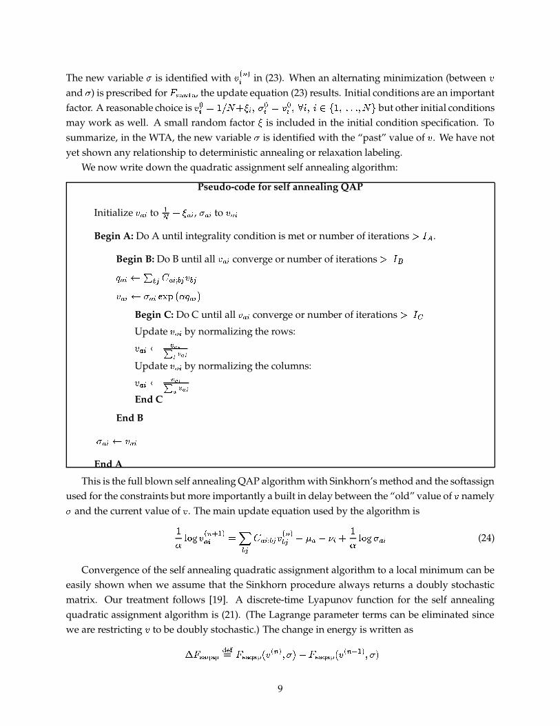
Pseudo-code for self annealing QAP

InitializeD � � to

�� I�� � � , � � � to

D � �Begin A: Do A until integrality condition is met or number of iterations -��� .

Begin B: Do B until allD � � converge or number of iterations -���

� � �� � � � ��� � D � D � �� � � � � "��># � � � ��.Begin C: Do C until all

D � � converge or number of iterations -����

UpdateD � � by normalizing the rows:D � �� ��� � � ��� �

UpdateD � � by normalizing the columns:D � �� ��� � � ��� �

End C

End B� � �� D � �End A

This is the full blown self annealing QAP algorithm with Sinkhorn’s method and the softassignused for the constraints but more importantly a built in delay between the “old” value of

Dnamely�

and the current value ofD

. The main update equation used by the algorithm is��OQP �8D � � � � �� � � 5 � � � ��� � D � � �� H # � H $

� I ��O P � � � � (24)

Convergence of the self annealing quadratic assignment algorithm to a local minimum can beeasily shown when we assume that the Sinkhorn procedure always returns a doubly stochasticmatrix. Our treatment follows [19]. A discrete-time Lyapunov function for the self annealingquadratic assignment algorithm is (21). (The Lagrange parameter terms can be eliminated sincewe are restricting

Dto be doubly stochastic.) The change in energy is written as

� ?��%B�� B ������ ?��%B���B �#%D � � � ����. H?��%B�� B! �#%D � � � � � ����.9

�*H �� 5� � � � � ��� � D � � �� � D �

� �� I �� 5 � �

D � � �� � OQP � D��� �� �� � �

I �� 5� � � � � ��� � D � � � � �� � D � ����� �� H �

� 5 � �D � ����� �� � OQP � D�� � � � �� �� � � (25)

The Lyapunov energy difference has been simplified using the relations � � D � � � �

. Using theupdate equation for self annealing in (24), the energy difference is rewritten as

� ?��EB�� B! � �� 5� � �

� � ��� � � D � � � D � I �� 5 � �

D�� � �� � OQP �D � � �� �D � � � � �� � � 9

(26)

where� D � � ������ D�� ����� �� � H�D�� � �� � . The first term in (26) is non-negative due to the positive definiteness

of � � ��� � � in the subspace spanned by the row and column constraints. The second term is non-

negative by virtue of being a Kullback-Leibler distance measure. We have shown the convergenceto a fixed point of the self annealing QAP algorithm.

5 Self annealing and deterministic annealing

Self annealing and deterministic annealing are closely related. To see this, we return to our favoriteexample—the winner-take-all (WTA). The self annealing and deterministic annealing WTAs arenow brought into accord: Assume uniform rather than random initial conditions for self anneal-ing.

D �,+ �� � � � � � =F� � ��� �� �+�����7�����. With uniform initial conditions, it is trivial to solve forD�� � �� : D�� � �� � � "�� # � �,�&� . � "�� # � �,� . �7= � ���1� �� � ������������� (27)

The correspondence between self annealing and deterministic annealing is clearly established bysetting

N�� ��� ��� � � � � �����

We have shown that the self annealing WTA corresponds to aparticular linear schedule for the deterministic annealing WTA.

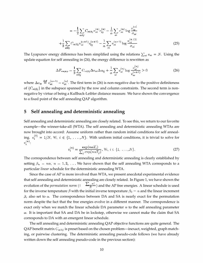
Since the case of AP is more involved than WTA, we present anecdotal experimental evidencethat self annealing and deterministic annealing are closely related. In Figure 1, we have shown the

evolution of the permutation norm#'�1H � � ���� �

� .and the AP free energies. A linear schedule is used

for the inverse temperatureN

with the initial inverse temperatureN + � � and the linear incrementN��

also set to�

. The correspondence between DA and SA is nearly exact for the permutationnorm despite the fact that the free energies evolve in a different manner. The correspondence isexact only when we match the linear schedule DA parameter

�to the self annealing parameter

�. It is important that SA and DA be in lockstep, otherwise we cannot make the claim that SA

corresponds to DA with an emergent linear schedule.The self annealing and deterministic annealing QAP objective functions are quite general. The

QAP benefit matrix� � ��� � is preset based on the chosen problem—inexact, weighted, graph match-

ing, or pairwise clustering. The deterministic annealing pseudo-code follows (we have alreadywritten down the self annealing pseudo-code in the previous section):

10

Self Annealing Deterministic Annealing

20 40 60 80 100 1200

0.05

0.1

0.15

0.2

0.25

0.3

0.35

0.4

0.45

0.5

iteration

perm

utat

ion

norm

α=0.5

α=1

α=5

Self Annealing Deterministic Annealing

0 5 10 15 20 25 30 35 40

−300

−280

−260

−240

−220

−200

−180

−160

iteration

assi

gnm

ent e

nerg

y

Figure 1: Left: 100 node AP with three different schedules. The agreement between self anddeterministic annealing is obvious. Right: The evolution of the self and deterministic annealingAP free energies for one schedule.

Pseudo-code for deterministic annealing QAP

InitializeN

toN + ,

D � � to�� I � � �

Begin A: Do A untilN � N��

Begin B: Do B until allD � � converge or number of iterations -���

� � �� � � � ��� � D � D � �� � "��># N � � �'.Begin C: Do C until all

D � � converge or number of iterations -����

UpdateD � � by normalizing the rows:D � �� ��� � � ��� �

UpdateD � � by normalizing the columns:D � �� ��� � � ��� �

End C

End B

N N � I NEnd A

Note the basic similarity between the self annealing and deterministic annealing QAP algo-rithms. In self annealing, a separation between past

#��7.and present

#%DF.replaces relaxation at a

fixed temperature. Moreover, in the WTA and AP, self annealing results in an emergent linearschedule. A similar argument can be made for QAP as well but requires experimental validation(due to the presence of bifurcations). We return to this topic in Section 7.

11

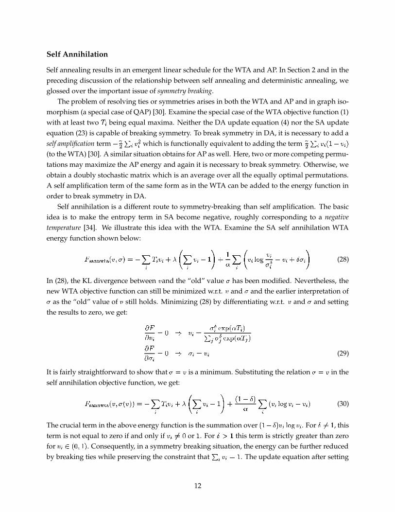
Self Annihilation

Self annealing results in an emergent linear schedule for the WTA and AP. In Section 2 and in thepreceding discussion of the relationship between self annealing and deterministic annealing, weglossed over the important issue of symmetry breaking.

The problem of resolving ties or symmetries arises in both the WTA and AP and in graph iso-morphism (a special case of QAP) [30]. Examine the special case of the WTA objective function (1)with at least two

�&�being equal maxima. Neither the DA update equation (4) nor the SA update

equation (23) is capable of breaking symmetry. To break symmetry in DA, it is necessary to add aself amplification term

H�� � � D �� which is functionally equivalent to adding the term� � � D � #��3H D � .

(to the WTA) [30]. A similar situation obtains for AP as well. Here, two or more competing permu-tations may maximize the AP energy and again it is necessary to break symmetry. Otherwise, weobtain a doubly stochastic matrix which is an average over all the equally optimal permutations.A self amplification term of the same form as in the WTA can be added to the energy function inorder to break symmetry in DA.

Self annihilation is a different route to symmetry-breaking than self amplification. The basicidea is to make the entropy term in SA become negative, roughly corresponding to a negativetemperature [34]. We illustrate this idea with the WTA. Examine the SA self annihilation WTAenergy function shown below:

?��%B���� @:ACB #ED&���7.��*H 5 � �&�%D/�FI J ' 5 � D<� H � * I �� 5 � ' D<�/OQP � D<����� H�D/�FI����F� * (28)

In (28), the KL divergence betweenD

and the “old” value�

has been modified. Nevertheless, thenew WTA objective function can still be minimized w.r.t.

Dand

�and the earlier interpretation of�

as the “old” value ofD

still holds. Minimizing (28) by differentiating w.r.t.D

and�

and settingthe results to zero, we get:

� ?� D/� � 9 D<�7� � �� � "�� # �,�&� . � � � "�� # �,� .� ?� �:� � 9 �F��� D/�

(29)

It is fairly straightforward to show that� � D

is a minimum. Substituting the relation� � D

in theself annihilation objective function, we get:

? �%B��� @:ACB #%D&���G#%D:.�.�� H 5 � �&�ED<� I J ' 5 � D/�&H � * I #�� H���.� 5 � #%D/�/OQP � D/�-H D/� .

(30)

The crucial term in the above energy function is the summation over#���H��M. D���OQP �8D<�

. For�� �*�

, thisterm is not equal to zero if and only if

D �� � 9or�. For

� - �this term is strictly greater than zero

forD � � # 9:�;�M.

. Consequently, in a symmetry breaking situation, the energy can be further reducedby breaking ties while preserving the constraint that

� D/��� �. The update equation after setting

12

50 100 150 200 2500

0.1

0.2

0.3

0.4

0.5

0.6

0.7

0.8

0.9

1

iteration number

perm

utat

ion

norm

0 50 100 150 200 250 30010

20

30

40

50

60

70

80

90

iteration number

AP

ene

rgy

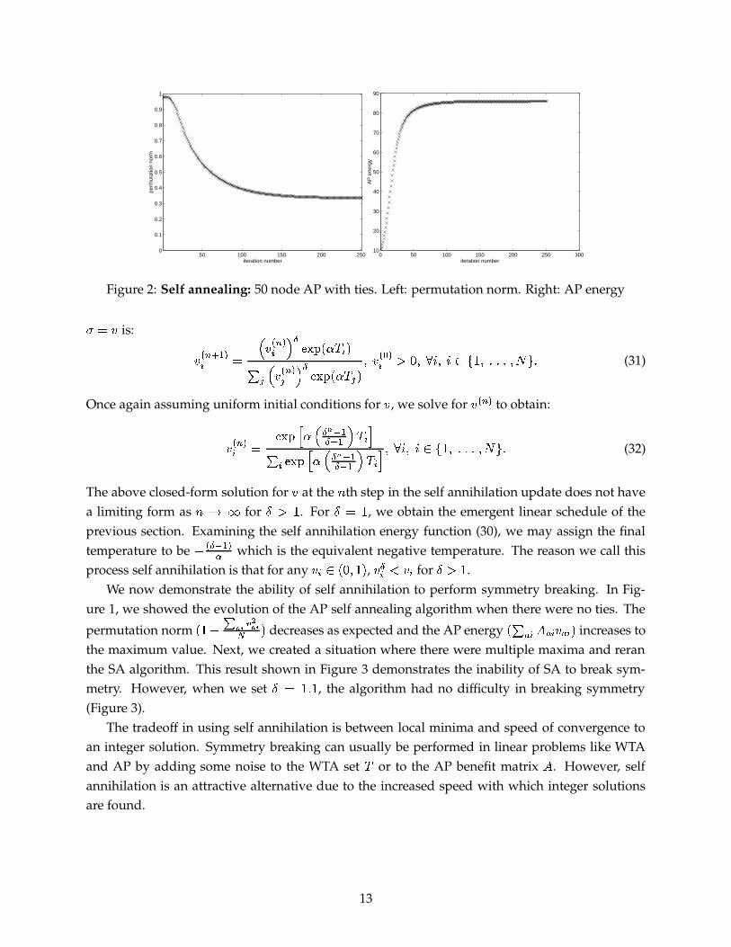
Figure 2: Self annealing: 50 node AP with ties. Left: permutation norm. Right: AP energy� � Dis:

D�� � � � �� � � D � � ���� � � "���# �-� �'. � D�� � � � � � "�� # �,� .

��D��,+ �� - 9:�7=F�������2�� ���������������(31)

Once again assuming uniform initial conditions forD

, we solve forD � � � to obtain:

D � � �� � � "������ � � ��� �� � � � � ��� � � "�� � � � � � � �� � � � �&� �

��=F��� ���2�� ���������������(32)

The above closed-form solution forD

at the � th step in the self annihilation update does not havea limiting form as � � for

� - �. For

� � �, we obtain the emergent linear schedule of the

previous section. Examining the self annihilation energy function (30), we may assign the finaltemperature to be

H � � � � �� which is the equivalent negative temperature. The reason we call thisprocess self annihilation is that for any

D � � # 9:�;�M.,D ��� D/� for

� - �.

We now demonstrate the ability of self annihilation to perform symmetry breaking. In Fig-ure 1, we showed the evolution of the AP self annealing algorithm when there were no ties. The

permutation norm#�� H � � � �� �

� .decreases as expected and the AP energy

# � � �"� �%D � �'. increases tothe maximum value. Next, we created a situation where there were multiple maxima and reranthe SA algorithm. This result shown in Figure 3 demonstrates the inability of SA to break sym-metry. However, when we set

�L� � �Q�, the algorithm had no difficulty in breaking symmetry

(Figure 3).The tradeoff in using self annihilation is between local minima and speed of convergence to

an integer solution. Symmetry breaking can usually be performed in linear problems like WTAand AP by adding some noise to the WTA set

�or to the AP benefit matrix � . However, self

annihilation is an attractive alternative due to the increased speed with which integer solutionsare found.

13

10 20 30 40 50 60 70 80 90 100 1100

0.1

0.2

0.3

0.4

0.5

0.6

0.7

0.8

0.9

1

iteration number

perm

utat

ion

norm

0 20 40 60 80 100 120−200

−150

−100

−50

0

50

100

iteration number

AP

ene

rgy

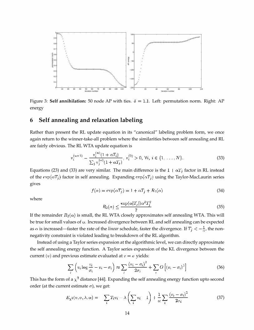
Figure 3: Self annihilation: 50 node AP with ties.�!� � �Q�

. Left: permutation norm. Right: APenergy

6 Self annealing and relaxation labeling

Rather than present the RL update equation in its “canonical” labeling problem form, we onceagain return to the winner-take-all problem where the similarities between self annealing and RLare fairly obvious. The RL WTA update equation is

D � � � � �� � D�� � �� #��1I��,�&� . ,D � � � #�� I��,� . ��D �,+ �� - 9:�-= � ���3�2�� �1�������������

(33)

Equations (23) and (33) are very similar. The main difference is the� I �,�

factor in RL insteadof the � "�� # �-� . factor in self annealing. Expanding � "�� # �,� . using the Taylor-MacLaurin seriesgives � # �8.�� � "�� # �,� .G�*�1I��,� I�� � # ��. (34)

where � � # ��.�� � "�� # ��� � � . � � � �� (35)

If the remainder� � # ��. is small, the RL WTA closely approximates self annealing WTA. This will

be true for small values of�

. Increased divergence between RL and self annealing can be expectedas�

is increased—faster the rate of the linear schedule, faster the divergence. If� H �� , the non-

negativity constraint is violated leading to breakdown of the RL algorithm.Instead of using a Taylor series expansion at the algorithmic level, we can directly approximate

the self annealing energy function. A Taylor series expansion of the KL divergence between thecurrent

#%DF.and previous estimate evaluated at

D � �yields:

5 �� D/�/O P � D/��:� H D/� I)�:� ��� 5 �

#%D/�-H �:� . �� �:� I 5 ��� � #%D/�&H �:� . �

(36)

This has the form of a � � distance [44]. Expanding the self annealing energy function upto secondorder (at the current estimate

�), we get:

��� � #%D&���-��J�� �8.3�*H 5 � �&�%D/� ILJ ' 5 � D/�,HL��* I �� 5 �

#ED/�-H �:� . �� �:� (37)

14

Self AnnealingEnergy Function

Self AnnealingDynamical System

Taylor seriesApproximation

Taylor seriesApproximation

Chi-SquaredEnergy Function

Relaxation LabelingDynamical System

Figure 4: From self annealing to relaxation labeling

This new energy function can be minimized w.r.t.D

. The fixed points are:

� �� D/� � 9 H �&�FI J I D/�&H �:��:� � 9� �� �:� � 9 �:�7� D/�

(38)

which after setting� � D � � � leads to

D�� ����� �� � D � � �� & � I�� #%�&�,H J&. ((39)

There are many similarities between (39) and (33). Both are multiplicative updating algorithmsrelying on the derivatives of the energy function. However, the important difference is that thenormalization operation in (33) does not correspond to the optimal solution to the Lagrange pa-rameter

Jin (39). Solving for

Jin (39) by setting

� D<�7�*�, we get

D�� � � �� � D�� � �� #'�1I �,�&� .8H � 5 � D�� � �(40)

By introducing the Taylor series approximation at the energy function level and subsequentlysolving for the update equation, we have obtained a new kind of multiplicative update algorithm,closely related to relaxation labeling. The positivity constraint is not strictly enforced in (40) asin RL and has to be checked at each step. Note that by eschewing the optimal solution to theLagrange parameter

Jin favor of a normalization, we get the RL algorithm for the WTA. The two

routes from SA to RL are depicted in Figure 4. A dotted line is used to link the � -squared energyfunction to the RL update equation since the normalization used in the latter cannot be derivedfrom the former.

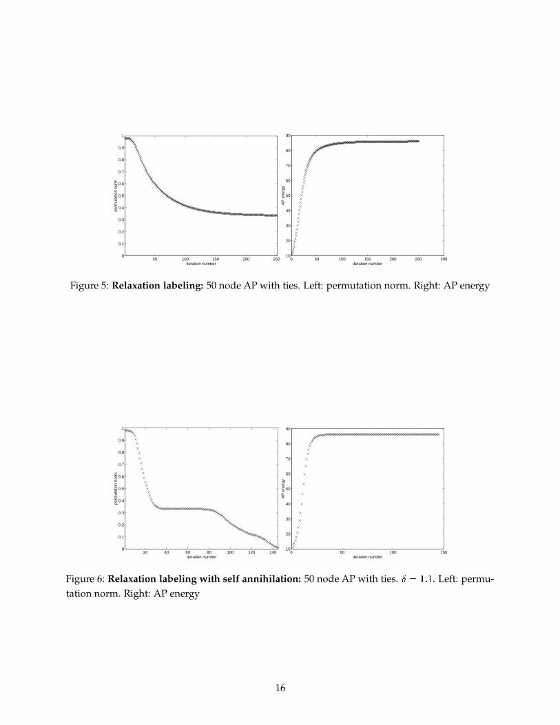
Turning to the problem of symmetry breaking, RL in its basic form is not capable of resolvingties. This is demonstrated in Figure 5 on AP. Just as in SA, self annihilation in RL resolves ties. In

Figure 6, the permutation norm#'� H � � � �� �

� .can be reduced to arbitrary small values.

15

50 100 150 200 2500

0.1

0.2

0.3

0.4

0.5

0.6

0.7

0.8

0.9

1

iteration number

perm

utat

ion

norm

0 50 100 150 200 250 30010

20

30

40

50

60

70

80

90

iteration number

AP

ene

rgy

Figure 5: Relaxation labeling: 50 node AP with ties. Left: permutation norm. Right: AP energy

20 40 60 80 100 120 1400

0.1

0.2

0.3

0.4

0.5

0.6

0.7

0.8

0.9

1

iteration number

perm

utat

ion

norm

0 50 100 15010

20

30

40

50

60

70

80

90

iteration number

AP

ene

rgy

Figure 6: Relaxation labeling with self annihilation: 50 node AP with ties.� �*� �Q�

. Left: permu-tation norm. Right: AP energy

16

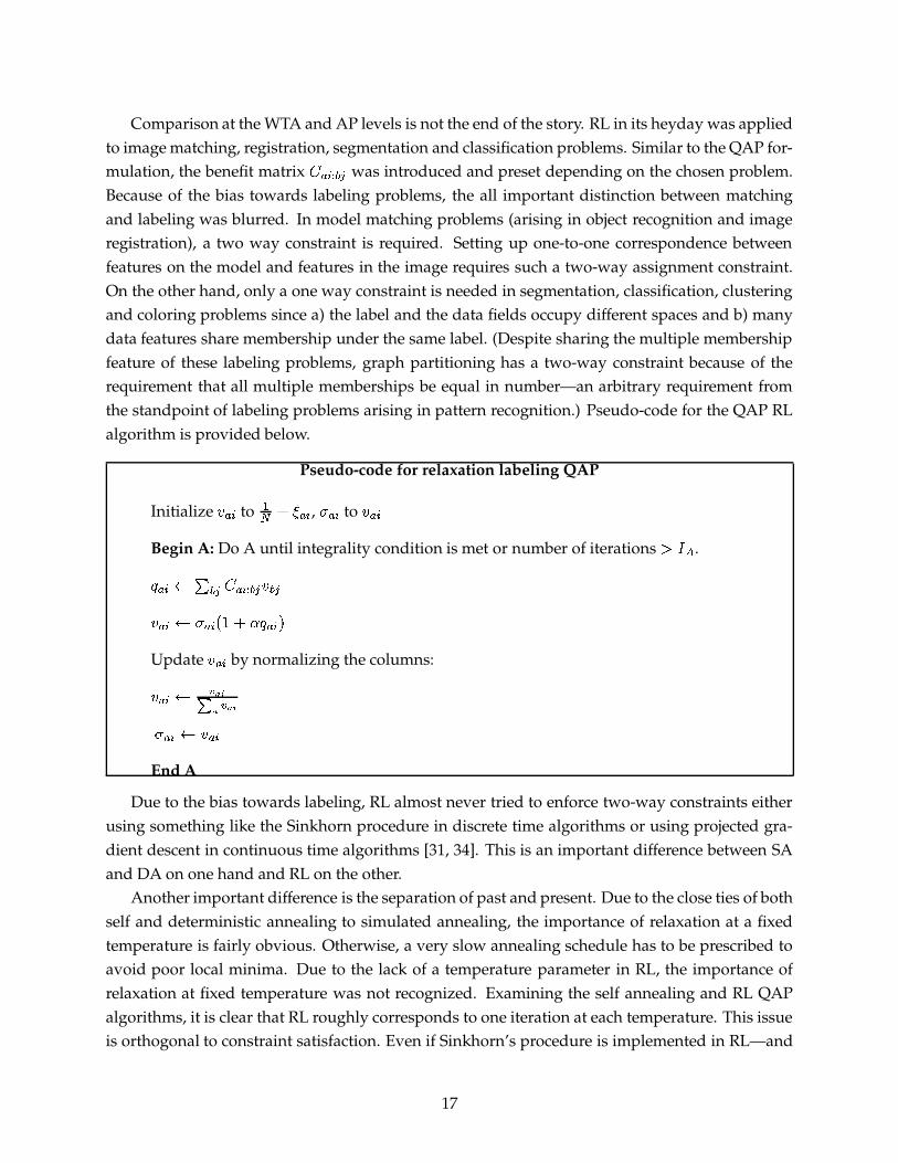
Comparison at the WTA and AP levels is not the end of the story. RL in its heyday was appliedto image matching, registration, segmentation and classification problems. Similar to the QAP for-mulation, the benefit matrix

� � ��� � was introduced and preset depending on the chosen problem.Because of the bias towards labeling problems, the all important distinction between matchingand labeling was blurred. In model matching problems (arising in object recognition and imageregistration), a two way constraint is required. Setting up one-to-one correspondence betweenfeatures on the model and features in the image requires such a two-way assignment constraint.On the other hand, only a one way constraint is needed in segmentation, classification, clusteringand coloring problems since a) the label and the data fields occupy different spaces and b) manydata features share membership under the same label. (Despite sharing the multiple membershipfeature of these labeling problems, graph partitioning has a two-way constraint because of therequirement that all multiple memberships be equal in number—an arbitrary requirement fromthe standpoint of labeling problems arising in pattern recognition.) Pseudo-code for the QAP RLalgorithm is provided below.

Pseudo-code for relaxation labeling QAP

InitializeD � � to

�� I�� � � , � � � to

D � �Begin A: Do A until integrality condition is met or number of iterations -��� .

� � �� � � � ��� � D � D � � � � �$#�� I�� � � �$.Update

D � � by normalizing the columns:

D � � � � � � � � �� � �� D � �End A

Due to the bias towards labeling, RL almost never tried to enforce two-way constraints eitherusing something like the Sinkhorn procedure in discrete time algorithms or using projected gra-dient descent in continuous time algorithms [31, 34]. This is an important difference between SAand DA on one hand and RL on the other.

Another important difference is the separation of past and present. Due to the close ties of bothself and deterministic annealing to simulated annealing, the importance of relaxation at a fixedtemperature is fairly obvious. Otherwise, a very slow annealing schedule has to be prescribed toavoid poor local minima. Due to the lack of a temperature parameter in RL, the importance ofrelaxation at fixed temperature was not recognized. Examining the self annealing and RL QAPalgorithms, it is clear that RL roughly corresponds to one iteration at each temperature. This issueis orthogonal to constraint satisfaction. Even if Sinkhorn’s procedure is implemented in RL—and

17

all that is needed is non-negativity of each entry of the matrix�7I ��� � � —the separation of past

#��7.and present

#%DF.is still one iteration. Put succinctly, step B is allowed only one iteration.

A remaining difference is the positivity constraint. We have already discussed the relationshipbetween the exponential and the RL term

#���I �,�-� .in the WTA context. There is no need to repeat

the analysis for QAP—note that positivity is guaranteed by the exponential whereas it must bechecked in RL.

In summary, there are three principal differences between self annealing and RL: (i) The pos-itivity constraint is strictly enforced by the exponential in self annealing and loosely enforced inRL, (ii) the use of the softassign rather than the softmax in matching problems has no parallel in RLand finally (iii) the discrete time self annealing QAP update equation introduces an all importantdelay between past and present (roughly corresponding to multiple iterations at each tempera-ture) whereas RL (having no such delay) forces one iteration per temperature with consequentloss of accuracy.

7 Results

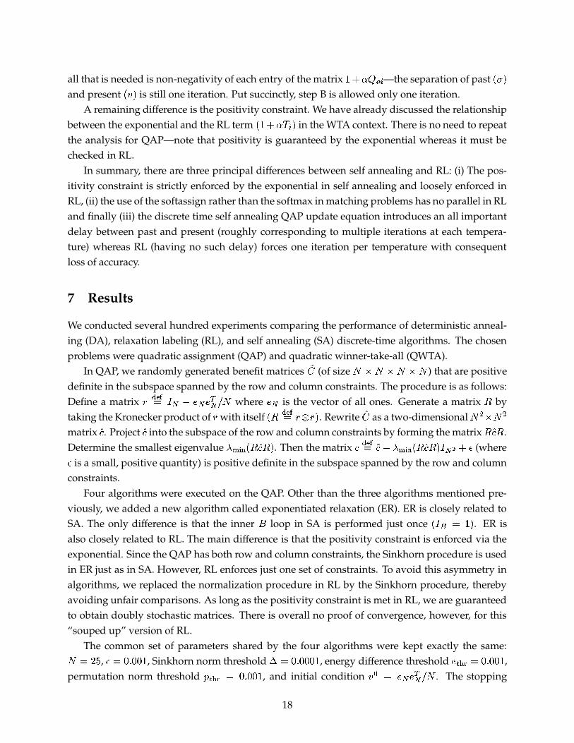
We conducted several hundred experiments comparing the performance of deterministic anneal-ing (DA), relaxation labeling (RL), and self annealing (SA) discrete-time algorithms. The chosenproblems were quadratic assignment (QAP) and quadratic winner-take-all (QWTA).

In QAP, we randomly generated benefit matrices �� (of size��� ��� ��� �

) that are positivedefinite in the subspace spanned by the row and column constraints. The procedure is as follows:Define a matrix �

������ � � H�� � �� � � � where� � is the vector of all ones. Generate a matrix

�by

taking the Kronecker product of � with itself# � ������

�� � . . Rewrite �� as a two-dimensional� ��� � �

matrix � . Project � into the subspace of the row and column constraints by forming the matrix� � � .

Determine the smallest eigenvalueJ ��� ��# � � �+. . Then the matrix ������ � H J ��� ��# � � �+. � � � I�� (where�

is a small, positive quantity) is positive definite in the subspace spanned by the row and columnconstraints.

Four algorithms were executed on the QAP. Other than the three algorithms mentioned pre-viously, we added a new algorithm called exponentiated relaxation (ER). ER is closely related toSA. The only difference is that the inner � loop in SA is performed just once

# � � � �M.. ER is

also closely related to RL. The main difference is that the positivity constraint is enforced via theexponential. Since the QAP has both row and column constraints, the Sinkhorn procedure is usedin ER just as in SA. However, RL enforces just one set of constraints. To avoid this asymmetry inalgorithms, we replaced the normalization procedure in RL by the Sinkhorn procedure, therebyavoiding unfair comparisons. As long as the positivity constraint is met in RL, we are guaranteedto obtain doubly stochastic matrices. There is overall no proof of convergence, however, for this“souped up” version of RL.

The common set of parameters shared by the four algorithms were kept exactly the same:��� ���,�3� 9:� 9 9:�

, Sinkhorn norm threshold� � 9:� 9 9 9:�

, energy difference threshold� A���� � 9:� 9 9:�

,permutation norm threshold

� A���� � 9:� 9 9:�, and initial condition

D + ��� � ��� � � � . The stopping

18

Self Annealing

Deterministic Annealing

Exponentiated Relaxation

Relaxation Labeling

10−2

10−1

100

101

450

460

470

480

490

500

510

520

QA

P m

inim

um e

nerg

y

α

Self Annealing

Deterministic Annealing

Exponentiated Relaxation

Relaxation Labeling

10−2

10−1

100

101

460

470

480

490

500

510

520

530

540

550

QW

TA

min

imum

ene

rgy

α

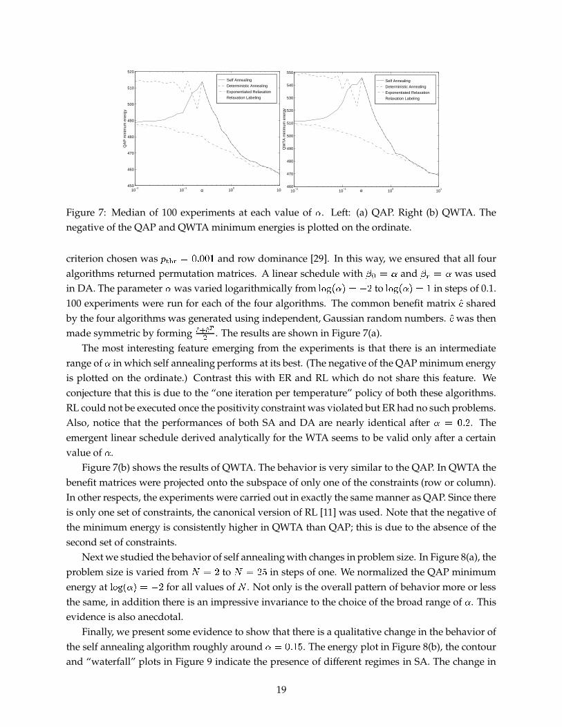
Figure 7: Median of 100 experiments at each value of�

. Left: (a) QAP. Right (b) QWTA. Thenegative of the QAP and QWTA minimum energies is plotted on the ordinate.

criterion chosen was� A���� � 9�� 9 9:�

and row dominance [29]. In this way, we ensured that all fouralgorithms returned permutation matrices. A linear schedule with

N + � � andN�� � �

was usedin DA. The parameter

�was varied logarithmically from

OQP �&# ��.G�*H �toOQP �&# �8. � �

in steps of 0.1.100 experiments were run for each of the four algorithms. The common benefit matrix � sharedby the four algorithms was generated using independent, Gaussian random numbers. � was thenmade symmetric by forming �

������� . The results are shown in Figure 7(a).

The most interesting feature emerging from the experiments is that there is an intermediaterange of

�in which self annealing performs at its best. (The negative of the QAP minimum energy

is plotted on the ordinate.) Contrast this with ER and RL which do not share this feature. Weconjecture that this is due to the “one iteration per temperature” policy of both these algorithms.RL could not be executed once the positivity constraint was violated but ER had no such problems.Also, notice that the performances of both SA and DA are nearly identical after

� � 9:� �. The

emergent linear schedule derived analytically for the WTA seems to be valid only after a certainvalue of

�.

Figure 7(b) shows the results of QWTA. The behavior is very similar to the QAP. In QWTA thebenefit matrices were projected onto the subspace of only one of the constraints (row or column).In other respects, the experiments were carried out in exactly the same manner as QAP. Since thereis only one set of constraints, the canonical version of RL [11] was used. Note that the negative ofthe minimum energy is consistently higher in QWTA than QAP; this is due to the absence of thesecond set of constraints.

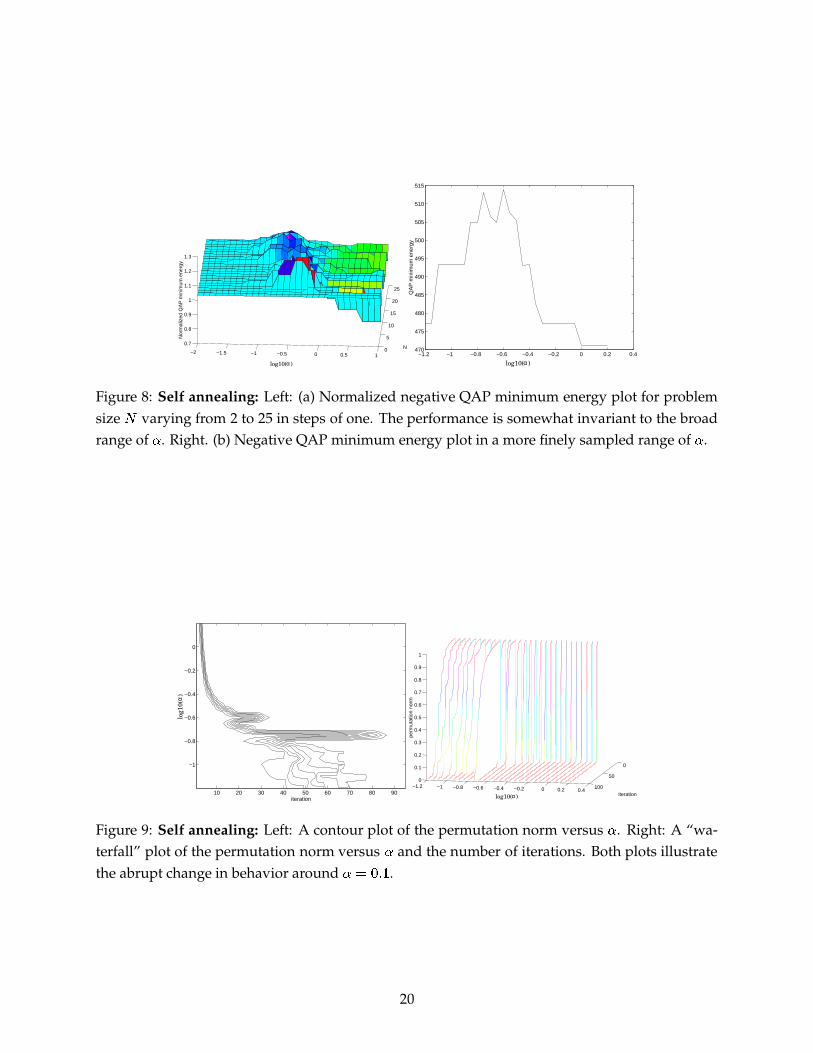
Next we studied the behavior of self annealing with changes in problem size. In Figure 8(a), theproblem size is varied from

� � �to� � ���

in steps of one. We normalized the QAP minimumenergy at

OQP � # ��. � H �for all values of

�. Not only is the overall pattern of behavior more or less

the same, in addition there is an impressive invariance to the choice of the broad range of�

. Thisevidence is also anecdotal.

Finally, we present some evidence to show that there is a qualitative change in the behavior ofthe self annealing algorithm roughly around

� � 9:�Q� �. The energy plot in Figure 8(b), the contour

and “waterfall” plots in Figure 9 indicate the presence of different regimes in SA. The change in

19

−2 −1.5 −1 −0.5 0 0.5 10

5

10

15

20

25

0.7

0.8

0.9

1

1.1

1.2

1.3

N

Nor

mal

ized

QA

P m

inim

um e

nerg

y

log10( α)

−1.2 −1 −0.8 −0.6 −0.4 −0.2 0 0.2 0.4470

475

480

485

490

495

500

505

510

515

QA

P m

inim

um e

nerg

y

log10( α)

Figure 8: Self annealing: Left: (a) Normalized negative QAP minimum energy plot for problemsize

�varying from 2 to 25 in steps of one. The performance is somewhat invariant to the broad

range of�

. Right. (b) Negative QAP minimum energy plot in a more finely sampled range of�

.

10 20 30 40 50 60 70 80 90

−1

−0.8

−0.6

−0.4

−0.2

0

iteration

log1

0( α

)

0

50

100−1.2 −1 −0.8 −0.6 −0.4 −0.2 0 0.2 0.4

0

0.1

0.2

0.3

0.4

0.5

0.6

0.7

0.8

0.9

1

iteration

perm

utat

ion

norm

log10( α)

Figure 9: Self annealing: Left: A contour plot of the permutation norm versus�

. Right: A “wa-terfall” plot of the permutation norm versus

�and the number of iterations. Both plots illustrate

the abrupt change in behavior around� � 9:�Q�

.

20

the permutation norm with iteration and�

is a good qualitative indicator of this change in regime.Our results are very preliminary and anecdotal here. We do not as yet have any understanding ofthis qualitative change in behavior of SA with change in

�.

8 Discussion

We have for the most part focused on the three way relationships between SA, DA and RL discretetime dynamical systems. One of the reasons for doing so was the ease with which comparisonexperiments could be conducted. But there is no reason to stop here. Continuous time projectedgradient dynamical systems could just as easily have been derived for SA, RL and DA. In fact,continuous time dynamical systems were derived for RL and DA in [3] and in [31, 45] respectively.In a similar vein, SA continuous time projected gradient descent dynamical systems can also bederived. It would be instructive and illuminating to experimentally check the performances ofthese continuous time counterparts as well as other closely related algorithms such as iteratedconditional modes (ICM) [46] and simulated annealing [47, 48] against the performances of thediscrete time dynamical systems used in this paper.

9 Conclusion

We have demonstrated that self annealing has the potential to reconcile relaxation labeling anddeterministic annealing as applied to matching and labeling problems. Our analysis also suggeststhat relaxation labeling can itself be extended in a self annealing direction until the two becomealmost indistinguishable. The same cannot be said for deterministic annealing since it has moreformal origins in mean field theory. What this suggests is that there exists a class of hithertounsuspected self annealing energy functions from which relaxation labeling dynamical systemscan be approximately derived. It remains to be seen if some of the other modifications to relaxationlabeling like probabilistic relaxation can be related to deterministic annealing.

References

[1] R. Duda and P. Hart. Pattern Classification and Scene Analysis. Wiley, New York, NY, 1973.

[2] A. L. Yuille and J. J. Kosowsky. Statistical physics algorithms that converge. Neural Computa-tion, 6(3):341–356, May 1994.

[3] R. Hummel and S. Zucker. On the foundations of relaxation labeling processes. IEEE Trans.Patt. Anal. Mach. Intell., 5(3):267–287, May 1983.

[4] J. J. Hopfield and D. Tank. ‘Neural’ computation of decisions in optimization problems.Biological Cybernetics, 52:141–152, 1985.

21

[5] G. Parisi. Statistical Field Theory. Addison Wesley, Redwood City, CA, 1988.

[6] A. L. Yuille. Generalized deformable models, statistical physics, and matching problems.Neural Computation, 2(1):1–24, 1990.

[7] K. Rose, E. Gurewitz, and G. Fox. Constrained clustering as an optimization method. IEEETrans. Patt. Anal. Mach. Intell., 15(8):785–794, 1993.

[8] J. S. Bridle. Training stochastic model recognition algorithms as networks can lead to max-imum mutual information estimation of parameters. In D. S. Touretzky, editor, Advances inNeural Information Processing Systems 2, pages 211–217, San Mateo, CA, 1990. Morgan Kauf-mann.

[9] A. Rangarajan, S. Gold, and E. Mjolsness. A novel optimizing network architecture withapplications. Neural Computation, 8(5):1041–1060, 1996.

[10] A. P. Dempster, N. M. Laird, and D. B. Rubin. Maximum likelihood from incomplete data viathe EM algorithm. J. R. Statist. Soc. Ser. B, 39:1–38, 1977.

[11] A. Rosenfeld, R. Hummel, and S. Zucker. Scene labeling by relaxation operations. IEEE Trans.Syst. Man, Cybern., 6(6):420–433, Jun. 1976.

[12] S. Peleg. A new probabilistic relaxation scheme. IEEE Trans. Patt. Anal. Mach. Intell., 2(4):362–369, Jul. 1980.

[13] O. Faugeras and M. Berthod. Improving consistency and reducing ambiguity in stochasticlabeling: an optimization approach. IEEE Trans. Patt. Anal. Mach. Intell., 3(4):412–424, Jul.1981.

[14] E. R. Hancock and J. Kittler. Discrete relaxation. Pattern Recognition, 23(7):711–733, 1990.

[15] W. J. Christmas, J. Kittler, and M. Petrou. Structural matching in computer vision usingprobabilistic relaxation. IEEE Trans. Patt. Anal. Mach. Intell., 17(5):749–764, Aug. 1995.

[16] M. Pelillo. Learning compatibility coefficients for relaxation labeling processes. IEEE Trans.Patt. Anal. Mach. Intell., 16(9):933–945, Sept. 1994.

[17] B. Kamgar-Parsi and B. Kamgar-Parsi. On problem solving with Hopfield networks. BiologicalCybernetics, 62:415–423, 1990.

[18] T. Hofmann and J. M. Buhmann. Pairwise data clustering by deterministic annealing. IEEETrans. Patt. Anal. Mach. Intell., 19(1):1–14, Jan. 1997.

[19] A. Rangarajan, A. L. Yuille, S. Gold, and E. Mjolsness. A convergence proof for the softassignquadratic assignment algorithm. In Advances in Neural Information Processing Systems 9, pages620–626. MIT Press, Cambridge, MA, 1997.

22

[20] C. Peterson and B. Soderberg. A new method for mapping optimization problems onto neuralnetworks. Intl. Journal of Neural Systems, 1(1):3–22, 1989.

[21] P. D. Simic. Constrained nets for graph matching and other quadratic assignment problems.Neural Computation, 3:268–281, 1991.

[22] S. Gold and A. Rangarajan. A graduated assignment algorithm for graph matching. IEEETransactions on Pattern Analysis and Machine Intelligence, 18(4):377–388, 1996.

[23] D. E. Van den Bout and T. K. Miller III. Graph partitioning using annealed networks. IEEETrans. Neural Networks, 1(2):192–203, June 1990.

[24] A. Rangarajan, H. Chui, E. Mjolsness, S. Pappu, L. Davachi, P. Goldman-Rakic, and J. Duncan.A robust point matching algorithm for autoradiograph alignment. Medical Image Analysis,4(1):379–398, 1997.

[25] S. Gold, A. Rangarajan, C. P. Lu, S. Pappu, and E. Mjolsness. New algorithms for 2-D and 3-Dpoint matching: pose estimation and correspondence. Pattern Recognition, 31(8):1019–1031,1998.

[26] D. E. Van den Bout and T. K. Miller III. Improving the performance of the Hopfield–Tankneural network through normalization and annealing. Biological Cybernetics, 62:129–139, 1989.

[27] P. D. Simic. Statistical mechanics as the underlying theory of ‘elastic’ and ‘neural’ optimisa-tions. Network, 1:89–103, 1990.

[28] D. Geiger and A. L. Yuille. A common framework for image segmentation. Intl. Journal ofComputer Vision, 6(3):227–243, Aug. 1991.

[29] J. J. Kosowsky and A. L. Yuille. The invisible hand algorithm: Solving the assignment prob-lem with statistical physics. Neural Networks, 7(3):477–490, 1994.

[30] A. Rangarajan and E. Mjolsness. A Lagrangian relaxation network for graph matching. IEEETrans. Neural Networks, 7(6):1365–1381, 1996.

[31] A. L. Yuille, P. Stolorz, and J. Utans. Statistical physics, mixtures of distributions, and the EMalgorithm. Neural Computation, 6(2):334–340, March 1994.

[32] W. J. Wolfe, M. H. Parry, and J. M. MacMillan. Hopfield-style neural networks and the TSP.In IEEE Intl. Conf. on Neural Networks, volume 7, pages 4577–4582. IEEE Press, 1994.

[33] A. H. Gee and R. W. Prager. Polyhedral combinatorics and neural networks. Neural Compu-tation, 6(1):161–180, Jan. 1994.

[34] K. Urahama. Gradient projection network: Analog solver for linearly constrained nonlinearprogramming. Neural Computation, 8(5):1061–1074, 1996.

23

[35] R. Sinkhorn. A relationship between arbitrary positive matrices and doubly stochastic matri-ces. Ann. Math. Statist., 35:876–879, 1964.

[36] A. K. Jain and R. C. Dubes. Algorithms for Clustering Data. Prentice Hall, Englewood Cliffs,NJ, 1988.

[37] J. Buhmann and T. Hofmann. Central and pairwise data clustering by competitive neuralnetworks. In J. Cowan, G. Tesauro, and J. Alspector, editors, Advances in Neural InformationProcessing Systems 6, pages 104–111. Morgan Kaufmann, San Francisco, CA, 1994.

[38] L. S. Davis. Shape matching using relaxation techniques. IEEE Trans. Patt. Anal. Mach. Intell.,1(1):60–72, Jan. 1979.

[39] L. Kitchen and A. Rosenfeld. Discrete relaxation for matching relational structures. IEEETrans. Syst. Man Cybern., 9:869–874, Dec. 1979.

[40] S. Ranade and A. Rosenfeld. Point pattern matching by relaxation. Pattern Recognition,12:269–275, 1980.

[41] K. Price. Relaxation matching techniques—a comparison. IEEE Trans. Patt. Anal. Mach. Intell.,7(5):617–623, Sept. 1985.

[42] M. Pelillo. On the dynamics of relaxation labeling processes. In IEEE Intl. Conf. on NeuralNetworks (ICNN), volume 2, pages 606–1294. IEEE Press, 1994.

[43] M. Pelillo and A. Jagota. Relaxation labeling networks for the maximum clique problem.Journal of Artificial Neural Networks, 2(4):313–328, 1995.

[44] J. Kivinen and M. Warmuth. Additive versus exponentiated gradient updates for linear pre-diction. Journal of Information and Computation, 132(1):1–64, 1997.

[45] K. Urahama. Mathematical programming formulations for neural combinatorial optimiza-tion algorithms. Journal of Artificial Neural Networks, 2(4):353–364, 1996.

[46] J. Besag. On the statistical analysis of dirty pictures. Journal of the Royal Statistical Society, B,48(3):259–302, 1986.

[47] S. Geman and D. Geman. Stochastic relaxation, Gibbs distributions and the Bayesian restora-tion of images. IEEE Trans. Patt. Anal. Mach. Intell., 6(6):721–741, Nov. 1984.

[48] S. Li, H. Wang, K. Chan, and M. Petrou. Minimization of MRF energy with relaxation label-ing. Journal of Mathematical Imaging and Vision, 7(2):149–161, 1997.

24