> '

IX

Dewey

HD28.M414

(^

Selecting Ingot Sizes for Joint Order Processing

in Sheet Manufacturing

Anantaram Balakrishnan

and

Srimathy Gopalakrishnan

WP# 3734-94-MSA October 1994

3F ~=r.-M-t-ZG •

W — W - -i- '>- <^^

Abstract

This paper addresses a tactical planning problem of seiecdng standard ingot sizes lo

facilitate joini processing of crders in a mate-to-order alunnrmm steet manafacniniig

operaiioiL Tne farilit}' has traditjonallv dedicated ingots to rodi'vidBal orders, bat is now

considaiiig producing multiple cffders from each ingot to reduce surplus and ejq>k>ii

ecoBomi^ of scale in processiag costs. Tie effectiveQess erf liiis jcani processing scras^zy

depends on ite a^.'silabk srapdard ingot sizes. We develc^ an integer programming mock:

to decide ingot sizes given tie disiiibimon of demand for various prodacis and the order

combination constraints. The model simultaneously addresses the issue of selecting a

prespecified number of standaid sizes luiiiile deciding whicii product combinaiions lo use.

The objective is to minimize tie total Tft'eigiii of ingots processed to saiisfv" demand for all

products. We describe a dual-ascent method to generate lower bounds for the probieiii sac

heuristic psrocedures to idendiS' good solutions. Extensive corc5>utaiiortal results nsmg

actual data from a leading aluminum shest manijfacturar confirm the effectri-eness of the

algorithm; on average the gaps bera-'een lie upper and lower bounds are abom 4%. Wealso illusuaie bow tfce nxxiel can be used to oerform sensidiirv^ analv'ses for lactica!

planning.

1. Introduction

This paper addresses a tactical planning problem in a leading aluminum sheet

manufacturing facility that produces sheet and plate products to customer specifications.

The problem, motivated by technological and market trends in the industry, deals with

selecting standard ingot sizes to produce multiple orders from a single ingot. The facility

produces ingots to stock in a few standard sizes. The downstream rolling mills use these

standard ingots to produce finished coils to order. To exploit the considerable economies

of scale in ingot casting and rolling costs, the facility has continuously upgraded its

equipment to produce and process larger ingots. At the same time, customers are placing

smaller orders more frequently to reduce their raw material inventories and move towards

just-in-time manufacturing. Consequently, the plant's traditional policy of dedicating an

ingot for each order is not economically viable. For instance, producing a 4,000 pound

order using a 10,000 pound ingot requires either storing the remaining 6,000 pounds of

finished product in stock or recycling this metal; furthermore, processing the 10,000 pound

ingot uses up scarce rolling mill capacity, possibly delaying other orders. To overcome

these problems, the plant is exploring the option of combining orders, i.e., jointly

producing multiple orders that require the same alloy and have similar specifications using

a single ingot. For a detailed discussion of the costs and benefits of order combination, see

Ventola [1991] and Balakrishnan and Brown [1992].

The choice of standard ingot sizes (widths and weights) determines the number of

available opportunities to combine orders, and thus greatly influences the cost

effectiveness of the order combination strategy. Reviewing and revising ingot sizes is a

medium-term (one to two years) decision since adding new standard ingot sizes requires

considerable lead time and investment to acquire and test new tooling. This paf>er

develops an optimization model to support this tactical ingot sizing decision. Tlie model

selects a prespecified number of standard ingot sizes to minimize the total weight of ingots

used to manufacture a representative mix of products for each alloy. Minimizing the total

ingot weight reduces processing time and costs as well as planned scrap and "surplus" (i.e.,

excess production that is not shipped). We formulate the problem as an integer program,

and develop an optimization-based solution procedure that combines dual ascent and

heuristics. Computational results using actual data from an aluminum sheet manufacturing

facility demonstrates that the solution procedure is quite effective, producing solutions that

are within 4% of optimality on average even without local improvement of the heuristic

solutions. For one product family that we analyzed, the new ingot sizes chosen by this

- 1

model provide savings of hundreds of thousands of dollars compared to using current ingot

sizes. We also use the model to study the sensitivity of ingot sizing decisions to various

technological and operational parameters.

This paper is organized as follows. Section 2 presents a brief description of the sheet

manufacturing process, defines the ingot sizing problem, and describes the integer

programming formulation. In Section 3, we develop a dual ascent procedure to compute

lower bounds and generate heuristic solutions. We also describe two stand-alone

heuristics. Section 4 provides details of our implementation and test problems, and

presents computational results and sensitivity analyses.

2. Problem Context and Formulation

2.1 Overview of sheet manufacturing process

Aluminum sheets have a variety of uses ranging from aerospace and automotive

applications to construction and packaging. The sheet manufacturing facility that we

studied produces a wide range of sheet and plate products to customer specifications.

These specifications include alloy, width, gauge (thickness), and total weight (or total

length). The facility maintains little or no uncommitted finished goods inventory. The

main steps in the sheet manufacturing process are ingot casting, hot rolling, cold rolling,

heat treatment, and finishing (e.g., slitting) operations.

Ingot casting consists of melting pure and scrap aluminum with the required alloying

elements, and pouring and cooling the molten metal to produce solid rectangular aluminum

ingots of the desired dimensions. This process requires separate tooling for each size, and

changing over production from one alloy and size to another entails long setup times and

wastage of metal (e.g., to flush the furnaces). Therefore, the ingot plant produces only a

limited set of standard sizes, primarily to stock, in large lots using a cyclic schedule.

Hot rolling, performed on reversing or multi-stand rolling mills, reduces the ingot's

thickness (and elongates it) at elevated temperatures. Cold rolling further reduces the

thickness to the desired finished gauge(s). A minimum amount of cold rolling is often

necessary to ensure that the product meets tight gauge and finish tolerances, and material

specifications (e.g., temper). Several cold rolling passes might be necessary if the finished

gauge is small relative to the sheet's thickness when it exits the hot mills. The width of the

sheet does not change during hot and cold rolling operations.

-2-

Although the number of ingot sizes is small, the facility is able to produce hundreds of

different finished specifications (width, gauge, and weight combinations) because the hot

and cold rolling operations are quite flexible, i.e., they can produce a wide range of

finished gauges from the same ingot, subject to width and weight restrictions.

Furthermore, the cold rolling process permits changing the gauge (during the final cold

rolling pass) while processing a coil, enabling the plant to jointly produce multiple orders

with comparable (but not necessarily identical) widths and gauges in a single coil (i.e.,

using a single ingot). Since the coil has uniform gauge until the final pass, and since the

amount of reduction in each pass is limited, the range of possible gauges in the finished

coil is limited. To account for this restriction, the plant has provided a "gauge combination

table" that specifies various gauge "windows" (or ranges) for each width. Two products

can be jointly produced from a single ingot only if both their gauges belong to one of these

windows.

One of the factors contributing to the scale economies in sheet production is the

"planned" scrap generated at various stages. For instance, ingots are "scalped" (a fixed

depth of material is removed from the top and bottom surfaces) prior to hot rolling.

Similarly, fixed lengths of the coil's leading and trailing ends (called head and tail scrap)

are discarded after rolling, and the sides of each coil need to be trimmed prior to shipping.

The proportion of metal lost due to "planned" scrap—scalping loss, head and tail scrap, and

side trim—decreases as the weight of the ingot increases.

Order combination, i.e., producing multiple orders using a single ingot, is advantageous

because it permits the facility to exploit economies of scale in processing large ingots and

also reduces the amount of surplus, i.e., excess quantity produced but not shipped to

customers. The surplus might be kept in inventory to satisfy some future order for the

same specification. To avoid accumulating uncommitted finished goods inventory, the

plant currently melts and reuses the surplus, incurring handling and reprocessing costs

(including melt loss). The plant's decision to explore order combination was prompted by

the increasing quantities of uncommitted metal (i.e., surplus) being recycled due to the

steady decrease in the quantity per customer order.

Combining up to three orders per ingot is apparently technically feasible (although not

actually tested in practice). However, the plant prefers not to combine more than two

orders for operational reasons, especially since order combination is a new and untested

strategy. We say an order pair is feasible if the two orders can be jointly produced using an

available ingot without violating any of the processing restrictions. In particular, the

following conditions must be met:

1. Alloy feasibility: Both orders require the same alloy.

2. Weightfeasibility: The sum of the weights of the two orders must be less than or equal

to the net weight (after subtracting the planned scrap allowances) of an available ingot

for that alloy;

3. Width feasibility: The width of each order must be less than or equal to the width of the

ingot minus the required side trim;

4. Gauge differential: The gauges of the two products must lie within one of the

corresponding gauge windows.

5. Width differential: The absolute difference in widths for the two orders must not

exceed a prespecified limit which we call the maximum width differential CO. This

operational restriction limits the amount of scrap (since the width of the ingot and coil

must exceed the larger of the two orders' widths). In our computational experiments,

we perform sensitivity analysis with respect to o).

We refer to these conditions collectively as the order combination rules. The weight

and width feasibility conditions imply that the feasibility of order pairs depends on the

available standard ingot sizes. Two orders might require the same alloy and have ;

compatible gauges and widths, and yet might not be feasible because none of the available

ingots for that alloy can accommodate both orders. Alternatively, an order pair might be

feasible, but combining them might require using a very large ingot (relative to the total

ordered weight); dedicating two smaller ingots to each order might then be more

economical. For dedicated ingots, i.e., producing a single order using an ingot, the net

weight and width of that ingot must equal or exceed the order weight and width.

In the short-run, given the set of standard ingot sizes, the scheduler must decide how to

combine the orders on hand and assign them to appropriate ingots. Ventola [1991 ] and

Gopalan [1992] discussed this decision problem, and observed that choosing good standard

ingot sizes can considerably improve short-run performance. This paper focuses on the

medium-term ingot sizing decision, namely, finding an effective set of standard ingot sizes

to facilitate short-run order combination. Since we cannot combine orders requiring

different alloys, the ingot sizing problem decomposes by alloy.

4-

2.2 Problem definition'^

For medium-term planning, we discretize the range of widths, gauges, and weights of

orders requiring a particular alloy, and consider all orders within each cell as a single

product group or product. Using past data on actual orders, we estimate the frequency of

orders or demand (number of orders) for each product. Ingots are specified by their alloy,

width, weight, and thickness (or length). We will focus on the ingot's width and weight

since only these two dimensions are relevant to test if an ingot can produce a particular

product pair (assuming this pair satisfies the gauge and width differential constraints).

Equipment capacities impose upper and lower limits on the ingot sizes. We assume that

the plant has identified a discrete set of candidate ingot sizes from this range. The ingot

plant also specifies the maximum number p of standard ingot sizes to select. Limiting

the number of standard ingot sizes has several advantages including reducing the

investment in tooling, limiting the number of changeovers and ensuring reasonably large

lot sizes, and reducing ingot safety stocks (and hence reducing both storage space

requirements and holding costs) due to the risk pooling benefits of having greater

commonality (see, for example. Baker, Magazine, and Nuttle [1986]). Our model does not

explicitly incorporate these factors; instead, by varying p, we can study the sensitivity of

the overall performance to this parameter.

Given the demand for each product, the parameters for the order combination rules, the

candidate ingot sizes, and the maximum number p of standard ingot sizes, the mgot sizing

problem (ISP) requires selecting p or fewer standard ingot sizes, and deciding the number

of ingots of each size to use for feasible product pairs (for the selected ingot sizes) or single

orders so as to meet the demand for all products. The objective is to minimize the total

planned scrap and surplus, or equivalently (since demand is fixed) to minimize the total

weight of ingots used.

The ISP combines two features—selecting p standard sizes, and "packing" orders in

ingots—that have been addressed separately in other contexts. Several papers have

addressed the problem of selecting standard lengths to stock and the related assortment

problem (e.g., Wolfson [1965], Pentico [1974], Beasley [1985], Pentico [1988]). This

problem deals with selecting standard sizes (e.g., lengths) for semi-finished items from a

given set of candidate sizes to meet demand for various finished sizes. The objective is to

minimize scrap and/or inventory holding and substitution costs. This class of models does

not consider order combination, i.e., it assumes that only one order can be produced from

each semi-finished item. For the one-dimension case, say, selecting standard lengths of

-5

steel rods, if we assume that a finished product with length / can be produced from any

semi-finished item with length greater than or equal to /, the problem can be solved

efficiently using dynamic programming (e.g., Pentico [1974]). Vasko, Wolf, and Stott

[1987] developed and applied a set covering approach to select optimal ingot sizes for the

steel industry. Again, their model did not incorporate the option of jointly producing

multiple orders using a single ingot. The literature on cutting stock problems considers the

issue of how to optimally "pack" multiple orders in available semi-finished sizes (e.g.,

Gilmore and Gomory [1961], [1963]). For instance, given rolls of certain widths and

lengths, the cutting stock problem selects an optimal set of patterns to produce all orders.

Chambers and Dyson [1976] and Beasley [1985] present heuristic algorithms for the two-

dimensional cutting stock problem with stock size selection.

2.3 Problem formulation

Let I = [1, ..., Ill} and K ={

1

IKI} respectively denote the index sets of products

and candidate ingot sizes. For all i g I, let d^ and Qj denote the demand and weight per

order for product i. For all k e K, let Wj^ denote the total weight of ingot type k. For every

pair of products i, j e I with i < j and every ingot type k e K, we apply the order

combination rules to determine if the pair (i,j) can be produced using ingot type k. Let UKdenote the set of all feasible assignments (i,j,k) such that the pair of products (i,j) can be

jointly produced using ingot type k. This set might include triplets such as (i,i,k) denoting

the assignment of two orders of product i to one type k ingot. We also include the option

of dedicating ingots: if a type k ingot can produce a single order of product i, we denote

this triplet as (0,i,k). (The index represents a dummy product that can be combined with

any single order, and has zero demand.) Notice that if, for some j e L the pair (i,j) is

feasible using ingot type k, then the pair (0,i) must also be feasible using ingot type k. Let

J(i) denote the set of all 'i-compatible" products, i.e., J(i) = {j: (i,j,k) or (j,i,k) g UK for

some k G K}

.

To formulate the ingot sizing problem, we define the following two sets of integer

variables:

f1 if ingot type k is chosen as a standard size, and . ,, , ^ ,

z. = \

to-'

^'

for all k G K; and,^ [0 otherwise

yjj,^= number of type k ingots used to produce product pair (i,j), for all (i,j,k) g UK.

For all i, j e L define X.jj = min { d,, d: } ; let X^ = d j for all products i. The ingot sizing

problem has the following integer programming formulation.

-6-

[ISP] Z* = min Z w^y.. (2.1)(i,j,k)eUK "^ 'J*^

subject to:

Demand constraints:

2 Z y::. + Z Z y-j, > d for all i e I (2.2)(i,i.k)€UK"^ j^i (i,j,k)eUK 'J" ^

Forcing constraints:

Maximum # of standard sizes:

Integrality/nonegativity:

y-^ < XjjZi^ forall(i,j,k)6UK, (2.3)

Z Zu < p, and (2.4)k€K "^

z^ = or 1 for all k e K (2.5a)

yy^ > and integer for all (i,j,k) € UK. (2.5b)

The objective function (2.1) minimizes the total weight of ingots used to satisfy the

demand for all products. Constraints (2.2) ensure that the demand for every product is

satisfied. The first term in the left-hand side of this equation represents the number of

ingots used to process the product-pair (i,i) if this pair is feasible for any ingot; each of

these ingots generates satisfies two units of demand for product i. The second term in the

left-hand side corresponds to the number of ingots containing one unit each of product i

(either dedicated or joint with some product j ^ i). The forcing constraint specifies that two

products i and j, with (i,j,k) e UK, can be jointly produced using ingot type k only if this

ingot type is chosen as a standard size. In this constraint, limiting the number of tyf)e k

ingots used to produce the pair (i,j) to at most \ (= min { dj, d: } ) is valid since (i,j,k) e

UK implies that (0,i,k) and (0,j,k) also belong to the set UK. Therefore, if a solution

assigns A.jj+5 ingots to the pair, (i,j) we can replace 5 of these pairs with single orders of

product i or product j depending on whether dj >dj. This change retains feasibility of the

solution, and does not increase the objective function value. Constraint (2.4) imposes the

upper limit of p on the number of standard sizes we select. We assume that [ISP] is

feasible (for instance, we can add a "large" ingot size to the candidate list such that

dedicating this ingot is feasible for every product).

The ISP is NP-hard since, as we note in the next section, the p-median problem (see,

for instance, Francis and Mirchandani [1990]) is a special case. Formulation [ISP] requires

-7-

prior enumeration of all feasible product pairs (i,j) for all candidate ingot sizes.

Consequently, the number of variables y--^ can be quite large. Instead, we might consider

directly encoding the product-pair feasibility rules as constraints in the problem

formulation. For instance, we can represent the problem as one of assigning products to

individual ingots, and checking the feasibility of assignments via constraints corresponding

to weight feasibility, width feasibility, gauge differential, and width differential. Our

solution procedure exploits the special structure of [ISP].

2.4 Special cases

Formulation [ISP] has two interesting special cases. First, suppose we do not permit

joint production, or the feasibility constraints are such that the pair (0,i) is the only feasible

"combination" for every product i. In this case, we can treat the products as "customers"

and candidate ingot sizes as "facilities" in a p-median problem. An ingot type k can ser\'e

product i only if (0,i.k) 6 UK. Note that, for a given choice of standard ingot sizes, the

problem has an optimal solution that assigns all dj units of product i to the same ingot type

k. The total surplus and planned scrap generated by this assignment, dj(wj, - q^), is the

"cost" of assigning product i to ingot type k. The p-median model selects at most p ingots,

and assigns products to ingots to minimize the total assignment cost.

The second special case, which we refer to as the order assignment problem,

corresponds to the situation when the standard ingot sizes are prespecified. or when IKI < p

(so [ISP] has an optimal solution with Zj. = 1 for all k € K). We can find the optimal y-

values for this special case by solving a non-bipartite matching problem defined over the

following network G; we later exploit this property in our heuristic solution procedure.

Figure 1 shows the network G for a 3 product, 3 ingot example. The network contains d^

nodes corresponding to each product i. We denote these nodes as (i,/) for / = 1 dj. If

the pair (i,i) is feasible using one of the available ingots, and if producing this pair is more

economical than dedicating two ingots to produce individual orders of product i. then we

add a single "dummy" node (i,dj+l). Otherwise, we say the pair (i,i) is dominated; in this

case, we add dj dummy nodes (i,/) for / = dj+l, ..., 2d|. For every feasible pair (i,j) (using

the available ingots) with i t^ 0, we connect every node (i,//; for /7 = 1 dj to every node

(j,/2) for 12 = 1, ..., dj. The cost of this edge is the weight of the best ingot for the pair (i,j),

i.e., the ingot k with the lowest weight such that (i,j,k)G UK; let kjj denote the index of this

ingot type. We also connect each node (i,//) for /7 = 1 dj to every dummy node (i,/2)

corresponding to product i; the cost of each of these edges is the weight of the lowest

I ._

weight ingot k^j that can produce a single order of product i. Finally, for each i e I, all

dummy nodes corresponding to product i are connected to each other with zero-cost edges.

The minimum-cost matching over G provides an optimal solution to the order

assignment problem. If a node (i,//j is connected to a node (j,l2) in the optimal matching,

then we assign one ingot of type kj: to the pair (i,j). If node (i,/) is connected to one of

product i's dummy nodes in the optimal matching, then we assign an ingot of type k^j to

produce a single order of product i. The total cost of the optimal matching equals the

optimal value of the order assignment problem. Finally, we can reduce the number of

edges in G by noting that for any subset of i-compatible products J' c J(i)\{0,i }, the

number of ingots assigned to produce the pairs (i,j) for all j e J' must not exceed the sum of

the demands for all products in J'. Suppose we index the products in J(i)\{0,i } in

increasing order of demand; then, for any j e J(i), we need to connect only the nodes (i,/)

for / = 1, ...., min {d:, 2- d:.) to all the nodes Q,12), for 12 = 1, ..., d:. This observationj'<jJ'eJ(i)

J J

reduces considerably the number of edges in G if a few products have high demands while

others have relatively low demands.

3. Solving the Ingot Sizing Problem

Since the ISP model is NP-hard, we focus on developing effective optimization-based

heuristics and lower bounds. This section describes a dual ascent method to generate lower

bounds on the optimal value, and heuristic methods (including a dual-based method) to

identify feasible solutions. These methods exploit the sp)ecial covering and p-median

features of formulation [ISP]. The gap between the lower bound and the best heuristic

solution value provides an assessment of the quality of the heuristic solution.

3.1 Dual ascent procedure

Dual ascent refers to a broad class of heuristic strategies to generate lower bounds as

well as feasible solutions by approximately solving the linear programming dual. This

technique has been successfully applied to several difficult discrete optimization problems

including the plant location problem (Erienkotter [1978]), the Steiner tree problem (Wong

[1984]), set packing problems (Fisher and Kedia [1986]), and the uncapacitated network

design problem (Balakrishnan, Magnanti, and Wong [1989]).

For the ISP, the value of any feasible LP dual solution provides a lower bound on the

optimal value Z*. Starting with a specific set of initial dual values, the dual ascent

procedure iteratively modifies these values in a myopic fashion to monotonically increase

the dual objective function value. The procedure terminates when no further myopic

improvement is possible. The final dual solution not only provides a lower bound, but also

suggests a partial solution to the original problem.

Consider the linear programming relaxation of formulation [ISP] obtained by replacing

the integrality restrictions (2.5a) and (2.5b) on the z and y variables with nonnegativity

constraints. Let Uj for all i e I, \-^ for all (i,j,k) e UK, and a be the dual variables

corresponding to the demand constraints (2.2), the forcing constraints (2.3), and the

maximum standard sizes constraint (2.4). Let U(k) = {(i,j): (i,j,k) € UK) denote the set

of all order pairs (i,j) that ingot k can produce. The linear programming dual [DISP] of

formulation [ISP] has the following form:

[DISP] Zp = max ZdjUj-pa (3.1)iel

subject to:

u, + Uj - w--^. < wj, for all (i,j,k) e UK, (3.2)

S X- V.,. - a < for all k G K, and (3.3)(ij)6U(k) y 'J*"

Uj > for all i 6 I, (3.4a)

Vjj^ > for all (i,j,k) 6 UK, (3.4b)

a > 0. (3.4c)

Note that constraints (3.2) corresponding to triplets (i,i,k) have the form:

2u,-v,^ < wj,.

To simplify the notation, we assume that formulation [DISP] also contains a dual variable

Uq corresponding to the dummy product 0, but we fix the value of Uq at zero.

Our dual ascent method exploits the following observations. Suppose we are given

nonnegative values for all the v-variables, say, v-jj^

for all (i,j,k) e UK. We wish to

A"complete" this partial solution V, i.e., determine values for a and the u-variables that are

feasible in [DISP] for the specified v-values, and maximize the dual objective function

10-

value. Since p > and since the objective function coefficient of a is -p, the "best" value

of a is the smallest value necessary to ensure feasibility of constraints (3.3), i.e..

a = MaxkeK (ij)eU(k)

^ij ^ijk (3.5)

Determining the best values of the u-variables is not as easy; however, we can identify

and exploit some properties that these values must satisfy. Let K(iJ) denote the subset of

ingots that can produce the pair (i,j). Since the u-values have positive coefficients in the

maximization objective function, the best values of the u-variables must be locally

maximum, i.e., we cannot increase one u-value without decreasing another. In particular,

for every product i e I, at least one constraint (3.2) containing the variable Uj must be^ A '^ A

"tight", i.e., if U = (uj) is an optimal completion of the partial solution (V, a) then:

Uj + U: = w.ijk

for at least one j e J(i) and k g K(i,j). (3.6)

Otherwise, we can increase some u-value without violating constraints (3.2); the new

solution has a higher dual objective function value. For all i e I and j g J(i), let

min (w^ + vjjk)k€ K(io)

(3.7)

Condition (3.6) implies that

(Ui + Uj) =5ij

for all i G I and j g J(i). (3.8)

For convenience, if the pair (i,i) is not feasible using any candidate ingot size, we will

assume b- = °°. Our dual ascent procedure iteratively changes the v-values, and

heuristically selects u-values to satisfy condition (3.8). We first describe how to select

initial values of the dual variables before discussing the multiplier adjustment methods and

the dual-based heuristic solution.

Initial dual solution

To construct an initial dual feasible solution, we select Vjj|^ = for all (i,j,k) g UK.

Consequently, a = 0. Assume, for convenience, that the products are indexed in order of

decreasing demand. To heuristically maximize the dual objective function value (for the

given v-values), we consider each product i in this decreasing-demand sequence, and set Uj

to its highest possible value given the prior choice of values U: forj= 1, ..., i-1. In

particular, we set:

11

u, = min { min (5 (iv Ji • min 5 }. (3.9)

j<i withj e J(i) " • ^ j>i with j e J(i) •*

This procedure ensures that the dual solution is feasible and satisfies condition (3.8).

The following procedure summarizes this dual initialization method.

Dual Initialization Method:

Step 1: Index the products from 1 to III in non-increasing order of demand dj.

Set Vjj^ <- for all (ij,k) e UK,

a <— 0, and

^D^ 0.

Step 2: Fori=l Ill, let

Hj = min I min [w,^] - U; }

;

j<i,jeJ(i) keK(i,j)

min [wj

112 = '^^'^^''2if i ^ J(»), and 00 otherwise;

113 = min { min [wJ }

;

j>i,jeJ(i) keK(iJ)

Set Uj <- min {|iJ,

112,1X3}, and

Next i;

When this procedure terminates, the final value of ^q is our initial lower bound on the

optimal value Z* of problem [ISP]. Next, we discuss how to improve this lower bound by

changing v-values, first one at a time and subsequently two values simultaneously.

Ascent procedure Phase 1 : Changing v-values one at a time

Increasing certain v-values might permit us to selectively increase u-values, and hence

the dual objective value. However, this increase might be offset by objective value

reductions due to required changes in other variables. For instance, increasing a particular

v-value might also require increasing a to maintain feasibility in constraints (3.3).

12

Likewise, when we increase one u-value, we might have to decrease other u-values to

maintain feasibility in constraints (3.2). Therefore, we must judiciously select the values to

increase so as to produce a net increase in the objective function value. The first phase in

our dual ascent procedure increases just one v-value at each iteration. We next motivate

and describe this procedure.

Let us first understand the implications of increasing the current value of a specific v-

variable, say, \ ^^. To facilitate our subsequent discussions, we define:

A = Set of all triplets (i,j,k) for which constraints (3.2) are tight.

B = Set of ingot types k for which constraints (3.3) are tight.

First, note that if the constraint (3.2) corresponding to a triplet (i,j,k) is not currently

tight, then the current Uj and U: values must be restricted by some other constraint(s) (3.2)

(assuming that these current values satisfy condition (3.8)). Therefore, increasing Vj:|.

does not create new opportunities to increase either Uj or u :. So, we consider only triplets

(i,j,k) in the set A.

Suppose we increase v j-,^ for one such triplet by A units. If k g B, then a must

correspondingly increase by X-A units to preserve feasibility of constraints (3.3), in which

case the dual objective function value decreases by pA^jjA. Otherwi.se (i.e., k ^ B), if Sj,

denotes the current slack in constraint (3.3) corresponding to ingot type k, a is unchanged

if we set A to be no more than s^-

.

Increasing Vj:,^ by A introduces a slack of A units in the corresponding constraint (3.2)

which we can use to increase either Uj or U:. (If i = j, we can increase Uj by only A/2 units.)

Suppose we select ujas the candidate variable to increase. Increasing its value by (= A if

i ^}, and A/2 if i = j) increases the dual objective function value by dj0 units. But, we

must also ensure that all other constraints (3.2) remain feasible. Consider any triplet (i,j',k')

e A\(iJ,k). Since the corresponding constraint (3.2) contains Uj in its left-hand side and is

tight, increasing Uj by requires decreasing U:. or increasing Vj:.^. by 0. Since Phase 1

increases only one v-value at a time, we ignore the latter option. Also, if j' = j, i.e., if two

or more constraints (3.2) corresponding to the product pair (i,j) are tight, then increasing Uj

requires decreasing Uj which implies that the original increase in Vj-^ is unnecessary. So,

we focus on product pairs (i,j) for which exactly one constraint (3.2) is tight. Since the u-

values must all be nonnegative, we cannot reduce u- by more than its current value Uj. i.e.,

must be less than or equal to u^. for all j' such that (i,j',k') e A\(i,j,k) for some k' e K.

13

For each such product j', reducing the value of U:. decreases the objective function value by

dj.0. Finally, for triplets (i,j',k') € A\(i,j,k:), increasing Uj does not require changes in other

u-values as long as is less than the current slacks in constraints (3,2) corresponding to

these triplets.

To summarize, we consider increasing one v-^ value, and if necessary (i.e., if k e B)

correspondingly increasing a to preserve feasibility of constraints (3.3). We increase Uj (or

U;), and identify other variables U:. belonging to tight constraints shared with Uj (or U:) that

must be reduced to preserve feasibility of constraints (3.2). Increasing Uj (or U:) increases

the dual objective function value, but compensating changes in the other variables reduce

this value. Furthermore, various factors limit the maximum possible change including the

slacks in constraints (3.2) that involve Uj (or U:) but are not tight, the slack in constraint

(3.3) corresponding to ingot type k, and the current values of the u-variables that must be

decreased. We evaluate the net change in the dual objective value for each triplet (i,j,k) €

A, and select the dual adjustment that produces the maximum increase. If none of the

adjustments produces a net increase in the dual objective function value, we terminate the

first phase. A formal description of the Phase 1 procedure follows:

Ascent procedure Phase 1

:

Step 1:

A = Set of triplets (i,j,k) for which constraints (3.2) are tight;

B = Set of ingot types k for which constraints (3.3) are tight;

Sj(^ = slack in the constraint (3.3) corresponding to ingot k, for all k € K.

For every (i,j,k) 6 A with (i,j,k') g A for any other k' e K(i,j),

For /= i,j,

let M = {m: (/, m, k') or (/, m, k') e A\(i,j,k)}.

Calculate maximum allowable value of 0:

0, = min u^;m e M

A A A A02 = min (w,^. + Vj.:.)^. -U-. - Uj.) ; and

(i'j',k')« A, i'orj' - I

^kAo = — ifke B, and oo otherwise.

hSet <— min { 0j,02, A3} ifi^^j, or

14

A,<- min { 0,,02, 2 )

if i=j-

Calculate net change in objective function value:

{d, - Z d^}0-Xijp3 ifke Bandi^tj,

me M

a..^(/) = {d,- Z d^}0-2Xijp0 ifkG Band i=j, and

me M

{d;- Z d^} ifk€ B.

me Mnext /;

next (ij,k);

Step 2:

Find the triplet (i,j,k) and / = i or j with maximum increase Ojj|^(0 in the dual objective

function value.

If this maximum increase is not positive, STOP.

Else, update

Uj <— U; + 0;

Uj^ <— Uj^ - for all m e M;

ifke B and i Ttj, a<— a+ A^j 0;

if ke B and i =j, a <— a + 2X^j 0; and.

Return to Step 1

.

Ascent Procedure Phase 2: Increasing two v-values simultaneously

In Phase 2, we evaluate ascent opportunities by simultaneously increasing two v-

values, Vjji^ and v-j^., for the same product pair (i,j) but different ingot types k and k'. As

before, we consider only triplets (i,j,k) and (i,j,k') that both belong to the set A of triplets

for which constraints (3.2) are tight. The procedure for increasing the two v-values is very

similar to the Pha.se 1 procedure, except that now we might have to decrease fewer u^^

values (since increasing the two v-values by creates a slack of units in two tight

constraints). If constraint (3.3) is tight for either k or k', then we must increase a.

Otherwi.se, the slack in these two constraints determines the maximum allowable increase

in the v-values. Other considerations that limit this allowable increase are the current

15

values of the variables u^ that need to be reduced (to preserve feasibility of tight

constraints involving u^), and the current slack in constraints that are not tight but contain

u^. We give below a formal description of this Phase 2 procedure.

Ascent procedure Phase 2:

Step 1:

A = Set of triplets (i,j,k) for which constraints (3.2) are tight;

B = Set of ingot types k for which constraints (3.3) are tight;

S|^ = slack in the constraint (3.3) corresponding to ingot k, for all k e FL

For every (i,j,k) and (i,j,k') € A,

For / = i, j,

let M = { m: (/, m, k") or (m, /, k") 6 A\{(i,j,k), (ij,k')}

}

Calculate maximum allowable value of O:

01 = min u^;m e M

©2 = min (w,^. + Vj.-^. - uj. - U;) ; and(i',j',k')g A, i'or j'= /

min (S|^,S|^)/>-j: if k and k' «E B,

A3 = Si^X^j (or Sj^/A^j ) if k (or k') € B and k' (or k) e B , and

00 otherwise.

orSet 0^ min { 0,,02, A3 } ifi^^^j,

<- min { 01,02, ^ } ifi=j.

Calculate net change in objective function value:

{d;- Z d^}0-X,jp0 ifkork'e Bandiv^j,me M

o,jy^.(/) = {d/- Z d^}0-2Xyp0 ifkork'e Band i=j, and

me M

{d,- Z dj„} if k and k' 6 B.mme M

next /;

next (i,j,k) and (i,j,k');

16

Step 2:

Find the triplets (i,j,k), (i,j,k') and / = i or j with maximum increase Oj:,j^.(0 in the dual

objective function value.

If this maximum increase is not positive, STOP.

Else, update

u^ <— U; + 0;

Uj^ <— Uj^ - for all m such that (/, m, k') g A\(i,j,k);

A A ^^Vijk^^jk + Q;

if k or k' e B and i ?tj, a <— a + X.^: 0; and,

if kork'e B and i =j, a <— a + lX^- 0; and.

Return to Step 1

.

Note that the same principle of increasing two v-values applies even to "unrelated"

triplets (i,j,k) and (i',j',k') belonging to the set A, possibly with i ^ i' and j ^j'. In this case,

when we increase v-. and v-:^., we must also decide whether to increase Uj or U: and u- or

Uj.. In our implementation, we consider only the special case with i = i' and j = j'.

If Phase 2 changes any of the dual values, then there might be opportunities to reapply

Phase 1 and further improve the dual objective function value. We continue alternating

between the Phase 1 and Phase 2 procedures until no further improvement is possible. The

final dual objective function value when the algorithm terminates is a lower bound on the

optimal value Z* of [ISP]. As we explain in the next section, we also use the final dual

solution to construct a feasible solution to the ingot sizing problem.

3.2 Heuristic procedures

This section describes three methods to select the standard ingot sizes—a dual-based

method, and two greedy heuristics. For each choice of standard ingot sizes, we solve the

order assignment problem (using a non-bipartite matching algorithm as described in

Section 2), and select the best solution as the ISP heuristic solution.

3.2.1 Dual-based heuristic solution

When the dual ascent procedure terminates, we try to construct a primal feasible

solution using complementary slackness conditions. If, in the final dual solution, the

constraint (3.3) corresponding to ingot type k is tight, then by complementary slackness

17-

ingot type k is a candidate for being included in the set of standard sizes. Hence, if the

dual ascent procedure ends with p or fewer constraints in the set (3.3) being tight, we

choose the ingots corresponding to these tight constraints as the standard ingots. We then

determine the optimal combinations and the actual solution value by solving the non-

bipartite matching subproblem as described in the Section 2. If more than p constraints in

(3.3) are tight at the end of the dual ascent phase, we select all the ingots corresponding to

the tight constraints as candidates for standard sizes. We then apply the greedy heuristics

that we describe next to select a subset of standard ingot sizes from this restricted set of

candidate ingots.

Given the set of candidate ingot sizes, the following two heuristics—the ingot

utilization heuristic and the greedy assignment heuristic—select standard ingot sizes one at

a time to heuristically minimize the total weight of ingots used. The heuristics differ in the

order in which they consider the candidate sizes.

3.2.2 Ingot Utilization heuristic

This heuristic attempts to select standard ingot sizes that can satisfy a large proportion

(in terms of weight) of the demand at high utilization levels. If we use an ingot type k to

produce the pair (i,j), the utilization of the ingot is the total weight (qj+q;) of the two orders

divided by the gross weight Wj^ of ingot k. Ideally, the chosen standard sizes and

combinations should be such that every ingot is nearly fully utilized. For this purpose, we

specify a threshold utilization level (}% (0 < (3 < 100) representing the minimum acceptable

ingot utilization. By parametrically varying p, we can generate multiple solutions.

The algorithm iteratively evaluates the total demand (in pounds) that every remaining

candidate ingot size can satisfy subject to the threshold utilization requirement, and selects

the size that satisfies the maximum demand. At any iteration, let K* and R denote the

current set of chosen and remaining candidate ingot sizes. The algorithm progressively

assigns demand for various products to the chosen sizes. Let &j denote the residual demand

(number of orders) for each product i g I. If ^j: = min {^j, &: }, we define the volume of a

product pair (i,j) as M(i,j) = ^j: (qj+q :). Let U(k) be the set of all product pairs that utilize a

type k ingot p% or more, i.e., U(k)= {(i,j): (i,j,k) e UK and (qj+qj) > |3w,/100}. Let

W(k) be the sum of volumes for all pairs (i,j) e U(k). The ingot utilization heuristic selects

the ingot k with maximum W(k) as the next candidate size, assigns all the product pairs

(i,j) e U(k) to this ingot, updates the residual demands, and repeats the procedure until p

candidate sizes are chosen. If at any stage, W(k) is zero for every remaining candidate size

18

k G ^ and if the demands are not completely satisfied, then we reduce the threshold value

P by a fixed percentage (10% in our computations) and continue the algorithm.

Ingot utilization heuristic:

Step 0: Initialize ^ <— set of candidate ingot sizes

K* <-({)

Sj = dj for all products i e I.

qj = weight per order of product i.

A

Step 1: For every k e K,

BU(k,p) = Set of all feasible pairs (ij) e U(k) with (qj+q^) >-^w,^.

lUU

i^. = min { dj , dj } for all (iJ) e U(k, p).

Compute W(k) = Z ^ij(qi + qj)(ij)eU(k,P)

next k;

Let k' = argmax { W(k): k e K }.

If W(k') = 0, update P <r- 0.90*p, and repeat Step 1.

Else, select ingot type k' as a standard ingot, i.e., update

K* <-K*u{k'};

K<-K\{k'};

dj <- max {dj - ^jj , 0} and dj <- max {dj - i-- , 0} for all (i,j) e U(k,P).

If IK*I = p or if d, = for all i g I, STOP. Else, repeat Step 1.

Step 2: For the chosen standard ingot sizes K*, solve the order assignment problem to

determine the optimal combinations.

3.2.3 Greedy Assignment heuristic

This heuristic attempts to first select good ingots for high-volume combinations. It

considers product pairs (i,j) in decreasing order of total weight, and selects the best ingotA

type for each pair in sequence. As before, let dj denote the residual demand for product i at

Aany intermediate iteration. Let U denote the set of feasible prtxluct pairs (i,j) such that the

A A A

residual demand for both i and j are positive. Define A,- = min {dj,d; } and volume M(i,j) =

A,jj {qj+q- } for every pair (i,j). Let K denote the current set of available candidate ingotA

sizes. We select the pair (i',j') e U with maximum volume M(i',j'), and determine the bestA

ingot k' G K for this combination, i.e., the ingot for which the scrap and surplus (w,^. - qj.-

- 19-

q:.) is minimum among all ingot types k e K. We add ingot type k' to the current set of

standard ingots, reduce the demands for products i' and j', and repeat the procedure until p

ingots have been selected or the residual demand for every product rs zero. This heuristic

strategy might be useful when the demand distribution is skewed, i.e., the demand for a

few products far exceeds other demands.

Greedy Assignment heuristic:

Step 0: Initialize ^ <— set of candidate ingot sizes

a, = dj for all products i € I

Let q jdenote the weight per order of product i.

Step 1: LI = set of all feasible pairs (i,j) with ^ and ^ > 0.AAA A

X- = min {dj, d: } for all (i,j) e U.

M(i,j)= l,j{q,-Kij} forall(i,j)eij.A

(i',j') = argmax {M(i,j) : i,j g LI }.

k' = argmin { (wj. - q,. - q. ) : ke R}.

Select ingot type k' as a standard ingot, i.e., update,

K*<-K*u{k'};

K^K\{k'};AAA AAAdj. <— dj. - AjY and d:. <— d:.- Aj.-. .

If IK*I = p or if dj = for all i e I, STOP. Else, repeat Step 1.

Step 2: For the standard ingot sizes K*, solve the order assignment problem to

determine the optimal combinations.

Several variants of these heuristics are possible. For instance, in the ingot utilization

heuristic, we might dynamically update the residual demand as we compute the total

weight W(k) of each candidate ingot. Likewise, in the greedy assignment method, for each

candidate ingot k we might consider the total weight of all combinations for which ingot k

is the best available ingot. We might also apply local improvement procedures to reduce

the total cost of each of these three heuristic solutions—the dual-ascent, ingot utilization,

or demand-based salutions. For instance, one procedure consists of considering each

current standard size in turn and evaluating the potential savings by replacing this size with

a neighboring (either larger or smaller) size. If none of these "swaps" produces any

-20

savings, the procedure terminates; otherwise, we perform the swap with maximum savings,

and repeat the procedure. To evaluate the savings for each swap, we solve the matching

problem to compute the total cost with the new proposed set of standard sizes (the total

cost is infmte if the new set of ingots cannot produce all products), and compare this cost

with the current cost.

In our computational experiments, we found that the best solution produced by the

three heuristics was itself quite close to optimality. So, we did not implement any local

improvement procedure.

4. Computational Results

We implemented and tested the dual ascent procedure and heuristics using data on

actual orders from a leading aluminum sheet manufacturer. We classified the orders into 4

distinct product groups, and separately solved the ingot sizing problem for each group. We

analyzed various scenarios obtained by varying the number of candidate ingot sizes, the

number of standard sizes required, and the maximum width differential. We also

compared the results with current practice and with restricted order combination options.

This section describes some implementation details and summarizes our computational

results.

4.1 Implementation details and test problems

We implemented the dual ascent procedure and heuristics in FORTRAN on an IBM

4381 computer. To solve the order assignment subproblem, we used Derigs' [1988] non-

bipartite matching algorithm.

We developed four test problems from a database of actual orders for a popular product

family (sheet products with gauges in a specified range and requiring a particular alloy)

over a 12-month period. The database contained over 500 "small" orders (i.e., orders for

which dedicating an ingot was not considered economical). We first classified these orders

into 4 natural product classes based on their widths. For one of these classes (Problem 3),

all products have the same width w; approximately 50% of the orders had this width. Wedivided the range of widths below w into two classes such that each class has

approximately equal number of products, and treat the range of widths above w as the

fourth class. Since products with large width differences (greater than the maximum width

differential parameter (d) cannot be combined, partitioning the data set into these four

-21

product classes does not eliminate many feasible pairs. Within each product class, we

selected appropriate intervals of widths, gauges, and weights to group the orders into

products. The width and weight intervals were defined by rounding up the actual order

widths and weights to the nearest inch and thousand pounds, respectively. The gauge

intervals corresponded to non-overlapping ranges from the table of feasible gauge

combinations (see Gopalakrishnan [1994] for additional details regarding the test

problems).

The facility currently produces ingots in 3 widths and a total of 6 standard sizes (width

and weight combinations). For each problem, we generated two sets of candidate ingot

sizes—a limited set and an extended set. The limited set has both fewer candidate widths

and fewer candidate weights for every width compared to the extended set. The number of

candidate weights for a particular width was chosen to reflect the relative demand for that

width. For instance, if many products have a width close to a candidate ingot width wl,

then for this width we might select candidate weights at 2,500 pound intervals in the range

of ingot weights that the ingot plant can produce; on the other hand, less popular widths

might have candidate weights at 10,000 pound intervals. Table 1 shows the number of

products and the number of candidate ingot sizes for both the limited and extended sets for

each of the four problems.

For the order combination constraints, we used the actual gauge combination table

supplied by the manufacturer. Our "standard" problems assume a maximum width

differential (o of 2 inches, i.e., we cannot combine two orders that differ in width by more

than 2 inches. We subsequently performed sensitivity analysis with respect to (O. To

compute the planned scrap allowances, we used the actual values of scalping loss, head and

tail scrap, and trim loss used by the planners. For each problem, we first generate all the

feasible combinations for every candidate ingot size based on the order combination

constraints, i.e., subject to the total weight, width, width differential, and gauge differential

restrictions. The demand for each product is the number of orders belonging to the

corresponding product group in our data set. Given the product demands, candidate ingot

sizes, feasible combinations, we obtain lower and upper bounds for various values of p by

applying the dual ascent procedure and heuristics. The integer programming formulation

for our largest test problem has 1 1096 variables and 1 11 66 constraints.

22-

4.2 Framework for experimentation

Our computational results seek to address two issues: (i) how effective are the dual

ascent and heuristic procedures in generating bounds and solutions; and, (ii) what is the

economic impact of changing the problem parameters. In all, we applied the dual ascent

and heuristic methods to over 80 problem instances.

We use the % gap between the upper and lower bounds, defined as (upper bound -

lower bound)* 100/lower bound, to assess algorithmic effectiveness. Low values of % gap

indicate that both the dual ascent lower bound is tight, and the heuristic procedures

perform well. For each problem instance, we select the best among the upper bounds

obtained by the heuristic procedures. Recall that the ingot utilization heuristic requires a

user-specified threshold utilization value p. We experimented with various values of P for

our standard test problems to identify effective settings for subsequent experimentation.

Section 4.3 reports these results on algorithmic effectiveness and compares the

performance of the heuristic solution procedures.

Section 4.4 illustrates how the ISP model and solution methodology can be used to

perform various types of sensitivity analyses. In particular, we explore the sensitivity of

the results to three problem features—the set of candidate ingot sizes, the number of

standard ingot sizes, and the maximum width differential parameter. We also compare the

total scrap and surplus when we permit order combinations with the results for two

restrictive scenarios: when we only permit dedicated ingots (i.e., one order per ingot), and

if we limit the combinations to identical orders. Finally, we compare the objective value

for the ISP solution with the corresponding value for the current set of standard ingot sizes

(but with order combination permitted).

4.3 Algorithmic effectiveness

We first compare the performance of various heuristics and determine an effective

range for the parameter P in the ingot utilization heuristic before assessing the quality of

the lower bounds.

4.3.1 Heuristic performance

To evaluate heuristic performance, we consider only problem instances with the

"standard" width differential of 2 inches and the limited set of candidate ingot sizes, but

several values for p. For the ingot utilization heuristic, we initially tried several threshold

utilization levels P ranging from 507o to 90%. Let us first understand how this parameter

-23-

might affect the quality of the solution. For high values of (3, relatively few pairs can

utilize an ingot P% or higher. Consequently, in the initial stages, the method might select

ingots that satisfy only a small proportion of the total demand. Subsequently, when this

threshold is no longer attainable for any remaining candidate ingot, the algorithm lowers

the threshold thus permitting less effective ingot sizes. At the other extreme, for low

values of (3, many pairs will achieve or exceed this threshold for every candidate ingot.

However, assigning these pairs reduces the overall average ingot utilization for the final set

of standard sizes. Therefore, for either extreme, we expect that the heuristic solution will

deteriorate. Our initial experiments confirmed this conjecture. For all our initial test

problems, the heuristic solution with p = 65, 70 or 80% was always better than the

solutions with P = 50 or 90%. So, we report results only for the former three values.

Table 2 shows the objective values for all four test problems for both the ingot

utilization heuristic, with P = 65, 70, and 80%, and for the greedy assignment heuristic.

Computation times (not reported here) for the heuristics were modest. Problems 1, 2, and

4 with a few hundred feasible assignments required 0.3 to 4.5 CPU seconds on an IBM

4381, whereas Problem 3 with several thousand feasible combinations required 30 to 50

CPU seconds. The results in Table 2 indicate that none of the methods is consistently

superior. Out of the 16 problem instances, the ingot utilization heuristic with P = 65% and

P = 80% produced the best solution in 5 instances each; the greedy assignment heuristic

and ingot utilization heuristic with P = 70% produced the best solution in 3 problem

instances each. In general, the ingot utilization heuristic performs better than the greedy

assignment method. The greedy method selects ingot sizes based on the residual volume

of a single product pair, whereas the ingot utilization heuristic considers multiple product

pairs that the ingot can produce. Indeed, the greedy assignment heuristic might sometimes

select small ingot sizes initially, making certain low-demand but "heavy-weight" products

infeasible at the end (after p standard sizes are selected). This phenomenon is apparent for

Problem 3, where the greedy heuristic failed to produce a feasible set of standard sizes for

values of p less than 6. In contrast, the ingot utilization heuristic has an adaptive feature

(reducing the threshold utilization level) to avoid infeasible solutions. Finally, in all of our

computational results, we observed that the dual-based heuristic solution often coincided

with the ingot utilization or greedy assignment solutions, but in no case was the dual-based

solution superior. We, therefore, do not separately report the results of this heuristic

method.

24-

For our subsequent experiments, we applied the ingot utilization heuristic, for all three

values of P, as well as the greedy assignment heuristic, and selected the best heuristic

solution value as the upper bound.

4,3.2 Dual ascent performance

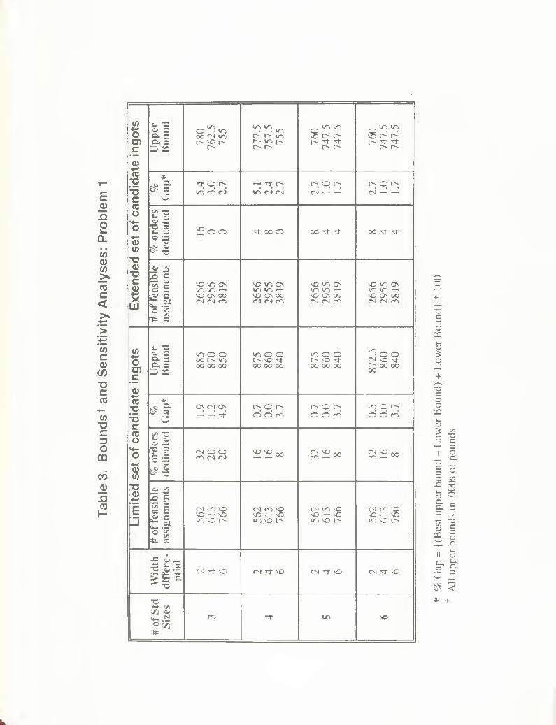
Tables 3 through 6 present the results for Problems 1 through 4, respectively, for

various p values and width differentials (except Problem 3 in which all products have the

same width) with both the limited and extended set of candidate ingot sizes. The tables

provide information on the respective problem sizes (# of feasible assignments) as well as

the % of orders processed using dedicated ingots in the best heuristic solution. The low %gaps in these tables show that the dual ascent lower bounds are tight, and the heuristic

solutions are near-optimal. In almost all problem instances, the % gap is below 7%. With

the limited set of candidate sizes, the average gap between the upper and lower bounds for

the four problems are 1.8%, 3.7%, 6.1%, and 4.7%, respectively. For the extended set of

candidate sizes, the corresponding averages are 2.7%, 3.0%, 4.9%, and 5.9%. Overall, the

procedure generates solutions that are (provably) within 4% on average.

In general, for a given width differential, the % gap tends to decrease as the number of

standard sizes p increases (except for Problem 3). However, increasing the width

differential or increasing the number of candidate ingot sizes (both of which increase the

number of feasible combinations) does not produce a similar consistent effect, e.g., in

Table 3 with the limited set of candidate ingots, for each value of p, the gap first decreases

and then increases as the width differential increases.

4.4 Sensitivity analyses

We now illustrate how to use the ISP model and methodology for planning and

decision support. In particular, we examine the sensitivity of the objective function value

to three problem features:

(i) the number of standard ingot sizes: Permitting more standard sizes enables the method

to choose sizes that are closer to the order combinations; consequently, the objective

function value should decrease;

(ii) the set of candidate ingot sizes: With more candidate sizes, the model has greater

choice in selecting a set of standard sizes, and hence we expect the total scrap and

surplus to decrease;

25

(iii) the width differential: Permitting greater differences in widths for combined orders

increases the number of feasible pairs, thus potentially reducing total pounds of metal

processed.

Tables 2 through 6 confirm these effects. For instance. Table 2 shows that as the

number p of standard ingot sizes increases from 3 to 6, the objective value decreases by up

to 2.7% (for Problem 3), assuming the standard width differential (2 inches) and for the

limited set of candidate ingot sizes. To assess the impact of increasing the set of candidate

ingot sizes consider, for instance. Problem 3 with p = 4. The objective function decreases

by 3.7% when we extend the set of candidate ingot sizes. Finally, increasing the width

differential appears to provide considerable benefits for Problems 1 and 4, but not so much

improvement for Problem 2 (for Problem 3, width differential is not relevant since all

products in this class have the same width). For instance, for Problem 4 with p = 3, the

objective value decreases by 10% when we increase the maximum width differential from

2 inches to 6 inches.

The tables also show the effect of increasing the maximum width differential parameter

(0 and extending the set of candidate ingot sizes on the size of the problem (measured by

the number of feasible assignments). Both of these changes increase the number of

feasible combinations; however, increasing the number of candidate sizes has much greater

impact on problem size. Also notice that, generally, as we extend the set of candidate

ingot sizes the % of orders with dedicated ingots in the best solution tends to decrease

(since more combinations are feasible); likewise, this % decreases as the width differential

increases.

4.5 Benefits of ingot sizing and order combination

To assess the benefits of order combination, we solved the ingot sizing problem for the

following two special cases : (i) no combinations permitted, i.e., all orders use dedicated

ingots, and, (ii) limited combinations, i.e., only dedicated ingots or combining two orders

for the same product are permitted. We also compare our proposed solution with the set of

standard sizes currently stocked by the facility. The results of all these experiments are

presented in the following sections.

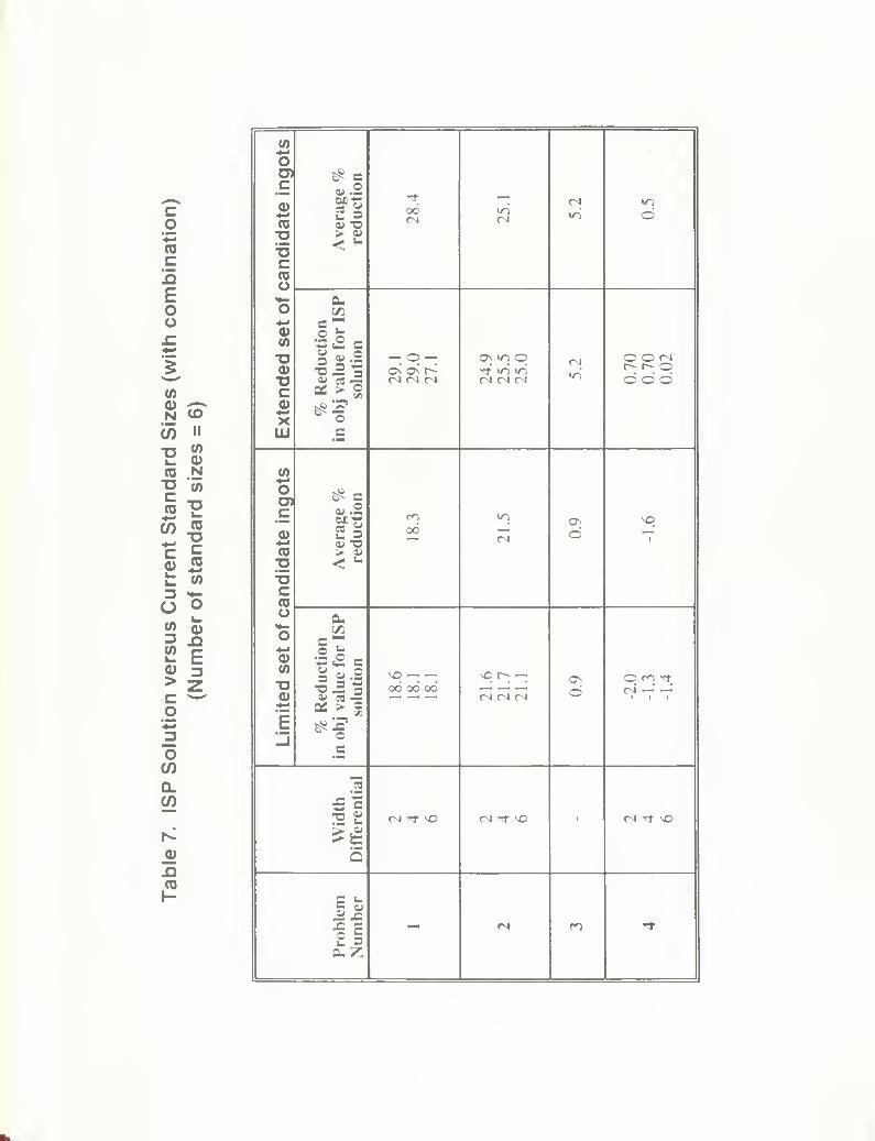
First, we compare the effectiveness of the ISP solution with the current set of standard

ingot sizes. The facility's cuaent 6 sizes, although not tailored for order combination, do

permit joint processing of orders. Using the matching procedure, we determined the

26

optimal assignment of feasible pairs to the current set of standard ingot sizes to meet total

demand. Table 7 compares the ISP values with the total weight of ingots processed for the

current ingot sizes (we compute the percentage deviation relative to the total weight for the

current sizes). For Problems 1 and 2, the ISP solution is considerably superior (over 1 8%

savings), whereas for Problems 3 and 4 the improvement is only marginal (indeed, for

Problem 4 with the restricted set of candidate ingots, the ISP solution is worse than current

practice; we attribute part of this deterioration to the poor quality of our heuristic solution).

Since all products in Problem 3 have the same width, solving the ISP does not produce

dramatic savings. When we extend the set of candidate ingot sizes, the savings are

uniformly higher, highlighting the importance of using a good set of candidate ingot sizes.

The total savings for the product family that we studied was of the order of hundreds of

thousands of dollars annually, and represented almost 10% reduction in the total weight of

metal processed.

To quantify the benefit of combining orders, we applied the ISP solution procedure to

two variants of Problem 3—one without any combinations (i.e., only dedicated ingots), and

one with limited combinations (within each product group only). Table 8 compares the

standard solution to these two special cases. The number of assignment variables increases

dramatically when we allow order combination, from 897 with no combinations to 1441

for limited combinations to 9838 for the standard model. In each case, we use our solution

methodology to determine a good set of standard sizes. Order combination allows us to

utilize the available ingots better, and reduces total surplus and scrap. The results indicate

that order combination reduces total ingot usage by an average of 8.3% when compared to

the limited-combinations model, and by an average of 26% when compared to the no-

combinations model.

5. Concluding Remarks

This paper has described the tactical planning problem of deciding standard ingot sizes

in a make-to-order aluminum sheet manufacturing facility. We modeled this problem as an

integer program, and developed a dual ascent lower bounding procedure and heuristics.

Our computational results indicate that the method is very effective, producing solutions

that are guaranteed to be within 4% of optimality. We also illustrated how to use the

model and solution method to assess the sensitivity of overall performance to problem

parameters such as the number of standard ingot sizes, the maximum width differential.

27

and the set of candidate ingot sizes. These results demonstrate that order combination is an

effective means to reduce total production costs.

Future work might address related algorithmic and practical issues, including

improving the two heuristic methods and exploring more sophisticated ascent methods to

increase several v-values simultaneously. In this paper we limited the number of orders

that can be combined to two, but combining more orders might become operationally

feasible in the future. The underlying dual ascent principles apply to this more complex

problem as well; however, the order assignment problem (for a given choice of standard

ingot sizes) is not as easy. Another issue to explore is the linkage between the medium-

term ingot sizing decisions and the short-term order combination decisions, perhaps, using

detailed simulations.

28

References

A. Balakrishnan, T. L. Magnanti, and R. T. Wong, 1989. A Dual Ascent Procedure

for Large scale Uncapacitated Network Design, Operations Research 37, 716-740.

A. Balakrishnan, and S. B. Brown, 1992. Process Planning for Metal-forming

Operations: An Integrated Engineering-Operations Perspective", Working Paper #

3432-92-MSA, Sloan School of Management, MIT, Cambridge, MA.

K. R. Baker, M. J. Magazine, and H. L. W. Nuttle, 1986. The Effect of Commonalityon Safety Stock in a Simple Inventory Model, Management Science 32, 982-988.

J. E. Beasley, 1985. An Algorithm for the Two-dimensional Assortment Problem,

European Journal of Operational Research 1 9, 253-26 1

.

M. L. Chambers and R. G. Dyson, 1976. The Cutting Stock Problem in Flat Glass

Industry - Selection of Stock Sizes, Operational Research Quarterly 27 , 949-957.

U. Derigs, 1988. Solving Non-bipartite Matching Problems via Shortest Path

Techniques, Annals of Operations Research 13, 225-264.

D. Erlenkotter, 1978. A Dual Based Procedure for Uncapacitated Facility Lxjcation,

Operations Research 26, 992-1009.

M. L. Fisher and P. Kedia, 1986. Optimal Solution of Set Covering/Partitioning

Problems using Dual Heuristics, Management Science 25, 955-966.

P. C. GiLMORE and R. E. Gomory, 1961. A Linear Programming Approach to the

Cutting Stock Problem, Operations Research 9, 849-859.

P. C. GiLMORE and R. E. Gomory, 1963. A Linear Programming Approach to the

Cutting Stock Problem, Part II, Operations Research 11, 863-888.

S. Gopalakrishnan, 1994. Optimization Models for Production Planning in Metal Sheet

Manufacturing, Unpublished thesis. Operations Research Center, MassachusettsInstitute of Technology, Cambridge, MA.

R. GoPALAN, 1992. Exploiting Process Flexibility in Metal Forming Operations,

Unpublished thesis. Operations Research Center, Massachusetts Institute of

Technology, Cambridge, MA.

R. L. FRANCIS and P. B. Mirchandani, 1990. Discrete Location Theory, John Wiley &Sons, Inc., New York.

D. W. Pentico, 1974. The Assortment Problem with Probabilistic Demands,,

Management Science 21, 286-290.

D. W. Pentico, 1988. The Discrete Two-dimensional Assortment Problem, OperationsResearch 36, 324-332.

F. J. Vasko. F. E. Wolf and K. L. Scott, 1987. Optimal Selection of Ingot Sizes via Set

Covering, Operations Research 35, 346-353.

D. P. Ventola, 1991 . Order Combination Methodology for Short-term Lot Planning at

an Aluminum Rolling Facility, Unpublished thesis, Massachusetts Institute of

Technology, Cambridge, MA.

M. L. WoLFSON, 1965. Selecting the Best Lengths to Stock, Operations Research 13,"

570-585.

R. T. Wong, 1984. Dual Ascent Approach for Steiner Tree Problems on a Directed

Graph, Mathematical Programming 28, 271-287.

E

Table 1. Problem Sizes

Problem

Number

E

o

m m

(00)w>.

COc<

(0c0)

(n

cCO

+-(0•ac3oCD

CO

0)

(0

(A

Oc0)-(0Dc(0uo0)(0

D0)T3C0)-XUJ

CM

Eono

(Ao(A>.

(0c<

COc0>(0

"OcCO-CO

c3om

onCO

I-

(0

E0)

noQ.

COa>0)>.

COc<

COc0)

(/)

DcCO•-COD

omCO0)

nCO

(0JoO)c<u<->

(0

c(0uo0)(0

XJ0)

T3c0)*•*

XLU

coOJc!5

Eou

(0(I)

--^N «>

(^ II

re N

re "2

(/) «

0) iSt w

o o(A A)

ifSio

o(/)

Q.if)

re

(0

oca>-t-t

re

"5

creuo%(0

T3Q)oc0)*-•

XMl

3 TDBO ODfiMbn? 1

CO

Eonoi-

Q.

Co(0c!o

Eoo0)T3

O

0)cVm00

0)

(0

%

Increase

in

obj

value

over

ISP

solution

>176 '^h^

Date Due

SEP. 6 199)

Lib-26-67