Selected Statistical Tests - WordPress.com · SEQUENTIAL TESTS ... Testing of Statistical...
258
-
Upload
hoangkhanh -
Category
Documents
-
view
270 -
download
3
Transcript of Selected Statistical Tests - WordPress.com · SEQUENTIAL TESTS ... Testing of Statistical...


This pageintentionally left
blank


Copyright © 2006 New Age International (P) Ltd., PublishersPublished by New Age International (P) Ltd., Publishers
All rights reserved.
No part of this ebook may be reproduced in any form, by photostat, microfilm,xerography, or any other means, or incorporated into any information retrievalsystem, electronic or mechanical, without the written permission of the publisher.All inquiries should be emailed to [email protected]
ISBN : 978-81-224-2429-4
PUBLISHING FOR ONE WORLD
NEW AGE INTERNATIONAL (P) LIMITED, PUBLISHERS4835/24, Ansari Road, Daryaganj, New Delhi - 110002Visit us at www.newagepublishers.com

PREFACE
Statistics is a subject used in research and analysis of data in almost all fields. Official governmentstatistics are our old records and creates historical evidences. Many people have contributed to therefinement of statistics, which we use today in various fields. It is a long process of development.
Today we have many statistical tools for application and analysis of data in various fields likebusiness, medicine, engineering, agriculture, management etc. Many people feel difficult to find whichstatistical technique is to be applied and where. Even though computer softwares have minimized thework, a basic knowledge is must for proper application.
This book is providing the important and widely used statistical tests with worked out examplesand exercises in real life applications. It is presented in a simple way in an understandable manner. Itwill be useful for the researchers to apply these tests for their data analysis. The statisticians also findit useful for easy reference. It is good companion for all who need statistical tools for their field.
The author is greatly indebted to the Authorities of Annamalai University for permitting topublish this book.
V. Rajagopalan

This pageintentionally left
blank
Preface ..................................................................................................................... v
1. INTRODUCTION..................................................................................................... 1-6
2. PARAMETRIC TESTS ............................................................................................7-93Test –1 Test for a Population Proportion ................................................................. 9Test – 2 Test for a Population Mean (Population variance is known) ..........................13Test – 3 Test for a Population Mean (Population variance is unknown) ......................16Test – 4 Test for a Population Variance (Population mean is known) ..........................20Test – 5 Test for a Population Variance (Population mean is unknown) .......................24Test – 6 Test for Goodness of Fit ..........................................................................27Test – 7 Test for Equality of two Population Proportions ..........................................30Test – 8 Test for Equality of two Population Means (Population variances
are equal and known) ...............................................................................33Test – 9 Test for Equality of two Population Means (Population variances
are unequal and known) ...........................................................................36Test – 10 Test for Equality of two Population Means (Population variances
are equal and unknown) ...........................................................................39Test – 11 Test for Paired Observations .....................................................................42Test – 12 Test for Equality of two Population Standard Deviations ..............................45Test – 13 Test for Equality of two Population Variances .............................................48Test – 14 Test for Consistency in a 2×2 table ...........................................................53Test – 15 Test for Homogeneity of Several Population Proportions .............................56Test – 16 Test for Homogeneity of Several Population Variances (Bartlett's test) ............60Test – 17 Test for Homogeneity of Several Population Means .....................................65Test – 18 Test for Independence of Attributes ...........................................................70Test – 19 Test for Population Correlation Coefficient Equals Zero ................................74Test – 20 Test for Population Correlation Coefficient Equals a Specified Value ..............78Test – 21 Test for Population Partial Correlation Coefficient ........................................81Test – 22 Test for Equality of two Population Correlation Coefficients .........................83Test – 23 Test for Multiple Correlation Coefficient .....................................................86
CONTENTS
viii Contents
Test – 24 Test for Regression Coefficient .................................................................88Test – 25 Test for Intercept in a Regression ..............................................................90
3. ANALYSIS OF VARIANCE TESTS ..................................................................... 95-153Test – 26 Test for Completely Randomized Design ....................................................97Test – 27 ANOCOVA Test for Completely Randomized Design ................................. 102Test – 28 Test for Randomized Block Design .......................................................... 109Test – 29 Test for Randomized Block Design .......................................................... 115
(More than one observation per cell)Test – 30 ANOCOVA Test for Randomized Block Design ......................................... 120Test – 31 Test for Latin Square Design ................................................................... 127Test – 32 Test for 22 Factorial Design .................................................................... 132Test – 33 Test for 23 Factorial Design .................................................................... 136Test – 34 Test for Split Plot Design ....................................................................... 141Test – 35 ANOVA Test for Strip Plot Design ........................................................... 148
4. MULTIVARIATE TESTS .................................................................................... 155-172Test – 36 Test for Population Mean Vectors (Covariance matrix is known) ................. 157Test – 37 Test for Population Mean Vector (Covariance matrix is known) .................. 160Test – 38 Test for Equality of Population Mean Vectors (Covariance matrices
are equal and known) ............................................................................. 164Test – 39 Test for Equality of Population Mean Vectors (Covariance matrices
are equal and unknown) ......................................................................... 167Test – 40 Test for Equality of Population Mean Vectors (Covariance matrices
are unequal and unknown) ...................................................................... 170
5. NON-PARAMETRIC TESTS ............................................................................. 173-210Test – 41 Sign Test for Median .............................................................................. 175Test – 42 Sign Test for Medians (Paired observations) ............................................. 177Test – 43 Median Test .......................................................................................... 179Test – 44 Median Test for two Populations ............................................................. 182Test – 45 Median Test for K Populations ................................................................ 184Test – 46 Wald–Wolfowitz Run Test ...................................................................... 187Test – 47 Kruskall–Wallis Rank Sum Test (H Test) .................................................. 189Test – 48 Mann–Whitney–Wilcoxon Rank Sum Test ................................................ 191Test – 49 Mann–Whitney–Wilcoxon U-Test ............................................................ 193Test – 50 Kolmogorov–Smirnov Test for Goodness of Fit ........................................ 197Test – 51 Kolmogorov–Smirnov Test for Comparing two Populations ........................ 199Test – 52 Spearman Rank Correlation Test .............................................................. 201Test – 53 Test for Randomness ............................................................................. 203Test – 54 Test for Randomness of Rank Correlation ................................................ 205Test – 55 Friedman's Test for Multiple Treatment of a Series of Objects .................... 207
Contents ix
6. SEQUENTIAL TESTS ........................................................................................ 211-224Test – 56 Sequential Test for Population Mean (Variance is known) ........................... 213Test – 57 Sequential Test for Standard Deviation (Mean is known) ............................ 216Test – 58 Sequential Test for Dichotomous Classification ......................................... 218Test – 59 Sequential Test for the Parameter of a Bernoulli Population ......................... 220Test – 60 Sequential Probability Ratio Test .............................................................. 223
7. TABLES .................................................................................................... 225-246
REFERENCES .................................................................................................. 247-248
Testing of Statistical hypotheses is a remarkable aspect of statistical theory, which helps us to makedecisions where there is a lack of uncertainty. There are many real life situations where we would liketo take a decision for further action. Further, there are some problems, for which we would like todetermine whether the claims are acceptable or not. Suppose that we are interested to test the followingclaims:
1. The average consumption of electricity in city ‘A’ is 175 units per month.2. Bath soap ‘B’ reduces the rate of skin infections by 50%.3. Oral polio vaccine is more potent than parenteral polio vaccine.4. A new variety of paddy yields 16.5 tones per hectare.5. Drug ‘C’ produces less drug dependence than drug ‘D’.6. Health drink ‘E’ improves weight gain by 25% for children.7. Plant produced by cloning grows 50% faster than the ordinary one.8. Door-to-door campaign increases the sales of a washing powder by 20%.9. Machine ‘F’ produces items within specifications than Machine ‘G’.
10. The defective items in a large consignment of coconut is less than 4%.These are a few of the many varieties of problems, which can be solved, only with the help of
statisticians. To solve such problems, we need the following basic and important concept in statisticstheory, as follows.
1. POPULATION
In any statistical investigation, the interest usually lies in the assessment of general magnitude withrespect to one or more characters relating to individuals belonging to a group. Such group of individualsunder study is called population. The number of units in any population is known as population size,which may be either finite or infinite. In a finite population, the size is denoted by, ‘N’. Thus instatistics, population is an aggregate of objects, animate or inanimate under study.
In statistical survey, complete enumeration of population is tedious, if the population size is toolarge or infinite. In some situations, even though, 100% inspection is possible, the units are destroyableduring the course of inspection. As there are various constraints in conducting complete enumerationnamely man-power, time factor, expenditure etc., we take the help of sampling.
INTRODUCTION
CHAPTER – 1
2 Selected Statistical Tests
2. SAMPLE
A finite, small subset of units of a population is called a sample and the number of units in a sample iscalled sample size and is denoted by ‘n’. The process of selecting a sample is known as sampling.Every member of a sample is called sample unit and the numerical values of such sample units arecalled observations. If each unit of population has an equal chance of being included in it, then such asample is called random sample. A sample of n observations be denoted by X1, X2,…, Xn.
3. PARAMETERS
The statistical measures namely mean, standard deviation, variance, correlation coefficient etc., if theyare calculated based on the population are called parameters. If the population information is neitheravailable completely nor finite, parameters cannot be evaluated. In such cases, the parameters aretermed as unknown.
4. STATISTICS
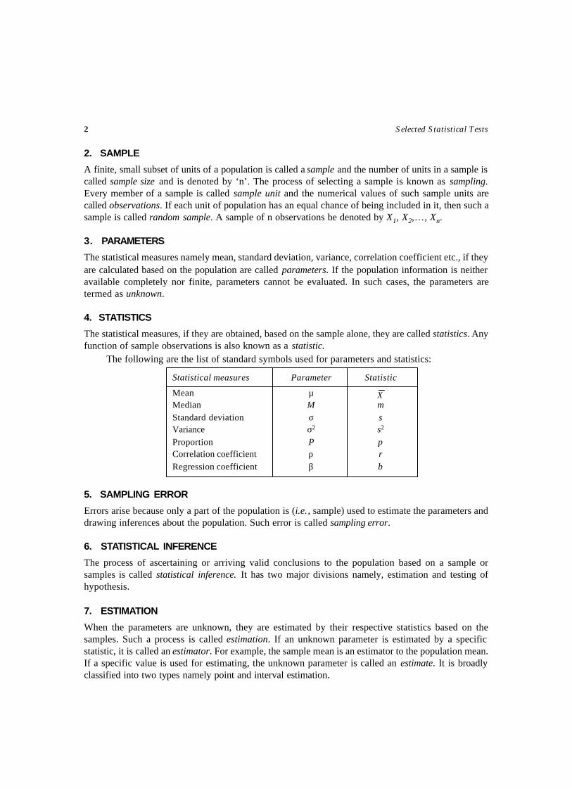
The statistical measures, if they are obtained, based on the sample alone, they are called statistics. Anyfunction of sample observations is also known as a statistic.
The following are the list of standard symbols used for parameters and statistics:
Statistical measures Parameter Statistic
Mean µ XMedian M mStandard deviation σ sVariance σ2 s2
Proportion P pCorrelation coefficient ρ rRegression coefficient β b
5. SAMPLING ERROR
Errors arise because only a part of the population is (i.e., sample) used to estimate the parameters anddrawing inferences about the population. Such error is called sampling error.
6. STATISTICAL INFERENCE
The process of ascertaining or arriving valid conclusions to the population based on a sample orsamples is called statistical inference. It has two major divisions namely, estimation and testing ofhypothesis.
7. ESTIMATION
When the parameters are unknown, they are estimated by their respective statistics based on thesamples. Such a process is called estimation. If an unknown parameter is estimated by a specificstatistic, it is called an estimator. For example, the sample mean is an estimator to the population mean.If a specific value is used for estimating, the unknown parameter is called an estimate. It is broadlyclassified into two types namely point and interval estimation.
Introduction 3
8. POINT AND INTERVAL ESTIMATION
If a single value is used as an estimate to the unknown parameter, it is called as point estimate and if wechoose two values a and b (a < b) so that the unknown parameter is expected to lie in between aand b. Such an interval (a, b), found for estimating the parameter is called as an interval estimate.
9. TESTING OF HYPOTHESIS
Hypothesis testing begins with an assumption or hypothesized value that we make about the unknownpopulation parameter. The sample data are collected and sample statistics are obtained from it. Thesestatistics are used to test the assumption about the parameter whether we made is correct. The differencebetween the hypothesized value and the actual value of the sample statistic is determined. Then wedecide whether the difference is significant or not. The smaller the difference, the greater the likelihood,that our hypothesized value is correct. We cannot accept or reject the hypothesized value about apopulation parameter simply by intuition. The statistical tests for testing the significance of the differencebetween the hypothesized value and the actual value of the sample statistic or the difference betweenany set of sample statistics are called tests of significance.
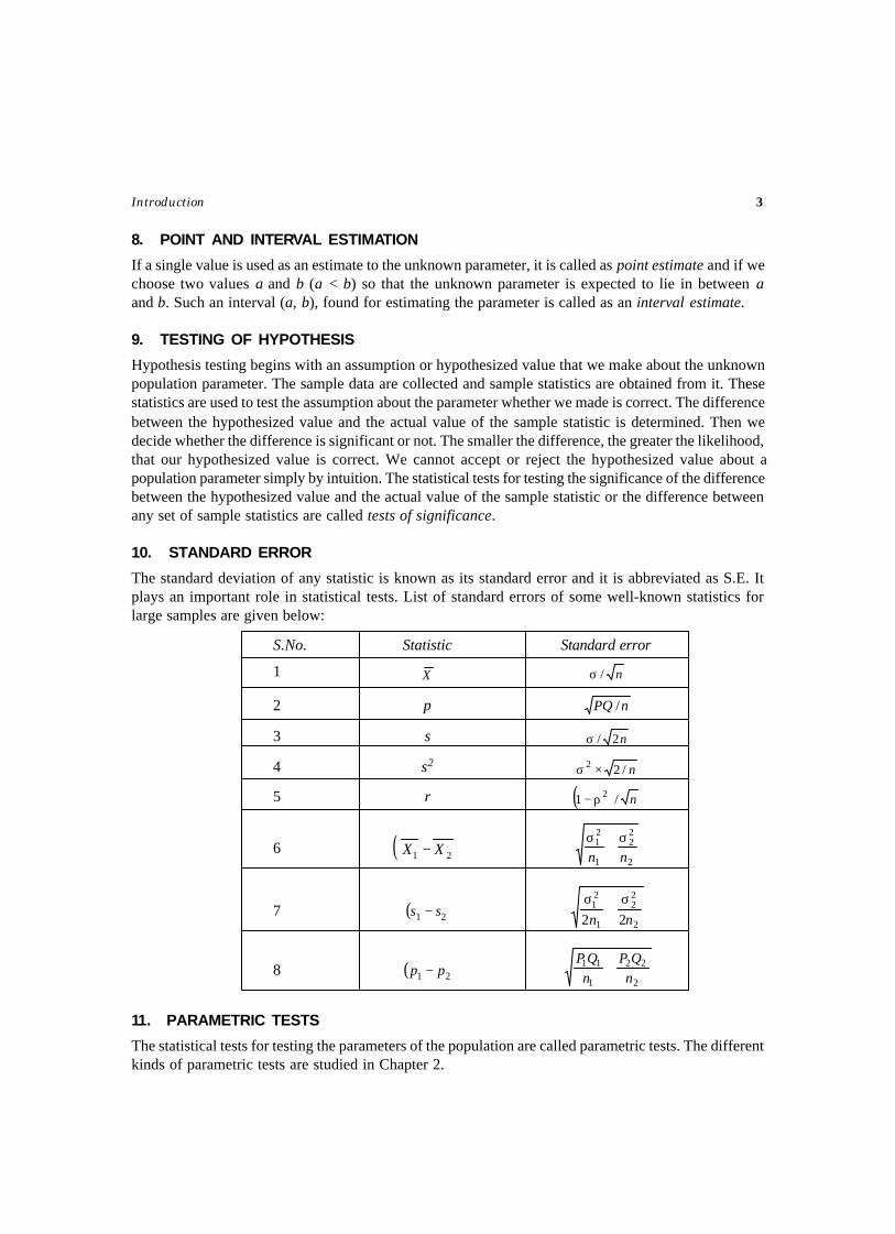
10. STANDARD ERROR
The standard deviation of any statistic is known as its standard error and it is abbreviated as S.E. Itplays an important role in statistical tests. List of standard errors of some well-known statistics forlarge samples are given below:
S.No. Statistic Standard error
1 X n/σ
2 p nPQ /
3 s n2/σ
4 s2 n/22 ×σ
5 r ( ) n/1 2ρ−
6 ( )21 XX − 2
22
1
21
nnσ+σ
7 ( )21 ss − 2
22
1
21
22 nn
σ+
σ
8 ( )21 pp − 2
22
1
11
nQP
nQP +
11. PARAMETRIC TESTS
The statistical tests for testing the parameters of the population are called parametric tests. The differentkinds of parametric tests are studied in Chapter 2.
4 Selected Statistical Tests
The following are the test procedures that we adopt in studying the parametric tests in a systematicmanner:
11.1 Null Hypothesis
It is a tentative statement about the unknown population parameter. It is to be tested based on thesample data. It is always of no difference between the hypothesized value and the actual value of thesample statistic. It is to be tested, for possible rejection under the assumption that it is true. It is usuallydenoted by H0.
11.2 Alternative Hypothesis
Any hypothesis, which is complementary to the null hypothesis, is called an alternative hypothesis. It isusually denoted by H1.
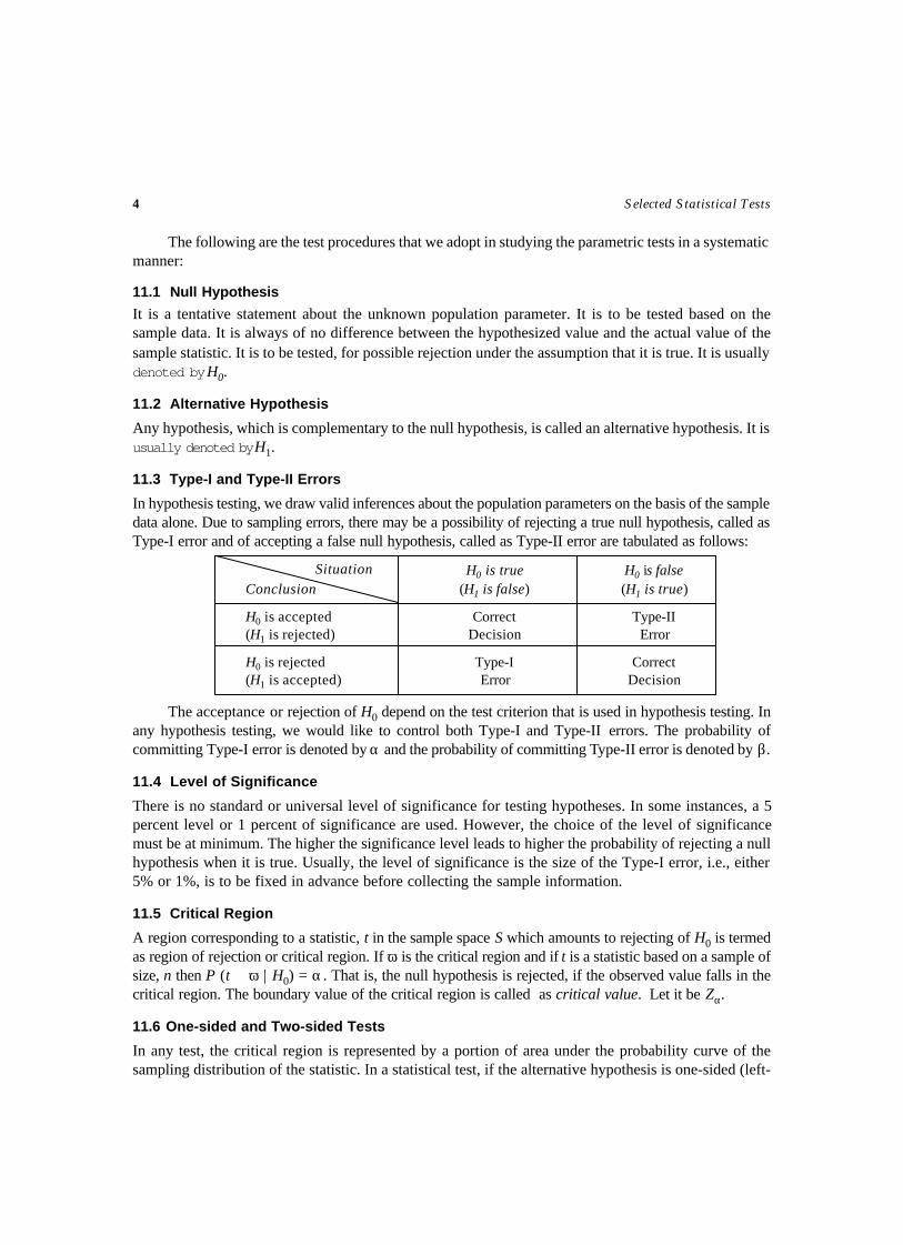
11.3 Type-I and Type-II Errors
In hypothesis testing, we draw valid inferences about the population parameters on the basis of the sampledata alone. Due to sampling errors, there may be a possibility of rejecting a true null hypothesis, called asType-I error and of accepting a false null hypothesis, called as Type-II error are tabulated as follows:
H0 is true H0 is falseConclusion (H1 is false) (H1 is true)
H0 is accepted Correct Type-II(H1 is rejected) Decision Error
H0 is rejected Type-I Correct(H1 is accepted) Error Decision
The acceptance or rejection of H0 depend on the test criterion that is used in hypothesis testing. Inany hypothesis testing, we would like to control both Type-I and Type-II errors. The probability ofcommitting Type-I error is denoted by α and the probability of committing Type-II error is denoted by β.
11.4 Level of Significance
There is no standard or universal level of significance for testing hypotheses. In some instances, a 5percent level or 1 percent of significance are used. However, the choice of the level of significancemust be at minimum. The higher the significance level leads to higher the probability of rejecting a nullhypothesis when it is true. Usually, the level of significance is the size of the Type-I error, i.e., either5% or 1%, is to be fixed in advance before collecting the sample information.
11.5 Critical Region
A region corresponding to a statistic, t in the sample space S which amounts to rejecting of H0 is termedas region of rejection or critical region. If ω is the critical region and if t is a statistic based on a sample ofsize, n then P (t ∈ ω | H0) = α . That is, the null hypothesis is rejected, if the observed value falls in thecritical region. The boundary value of the critical region is called as critical value. Let it be Zα.
11.6 One-sided and Two-sided Tests
In any test, the critical region is represented by a portion of area under the probability curve of thesampling distribution of the statistic. In a statistical test, if the alternative hypothesis is one-sided (left-
Situation
Introduction 5
sided or right-sided) is called a one-sided test. For example, a test for testing the mean of a population,H0: µ = µ0 against the alternative hypothesis H1: µ < µ0 (left-sided) or H1: µ > µ0 (right-sided) and fortesting H0 against H1: µ ≠ µ0 (two-sided) is known as two-sided test.
11.7 Test Statistic
A statistical test is conducted by means of a test statistic for which the probability distribution isdetermined by the assumption that the null hypothesis is true. It is based on the statistic, the expectedvalue of the statistic (hypothesized value assumed in H0) and the standard error of the statistic. Thevalue so obtained as test statistic value based on the observed data is called observed value of the teststatistic, let it be Z, and we use this value for arriving conclusion.
11.8 Conclusion
By comparing the two values namely, the observed value of the test statistic and the critical value, theconclusion is arrived at.
If Z ≤ Zα, we conclude that there is no evidence against the null hypothesis H0 and hence it maybe accepted.
If Z > Zα, we conclude that there is evidence against the null hypothesis H0 and in favor of H1.Hence, H0 is rejected and alternatively, H1 is accepted.
12. ANALYSIS OF VARIANCE
It is a powerful statistical tool in tests of significance. In parametric tests, we discussed the statisticaltests relating to mean of a population or equality of means of two populations. In situations, when wehave three or more samples to consider at a time, an alternative procedure is needed for testing thehypothesis that all the samples are drawn from the same populations, which have the same mean.
Analysis of variance (ANOVA) was introduced by R.A. Fisher to deal the problem in the analysisof agricultural data. Variations in the observations are inherent in nature. The total variation in theobserved data is due to the following two causes namely, (i) assignable causes, and (ii) chance causes.By this technique, the total variation in the sample data can be bifurcated into variation between sampleand variation within samples. The second kind of variation is due to experimental error.
These kinds of tests are very much applicable in agricultural field experiments, where they wantto know the yield of different kinds of seeds, fertilizers adopted, pesticides used, different irrigation,cultivation method etc., accordingly there are different types of ANOVA tests available and are providedin Chapter 3.
In ANOVA tests, we need the following terms with their definitions:
12.1 Treatments
Various factors or methods that we adopted in a comparative experiment are termed as treatments. Forexample, in field experiments, different varieties of paddy seeds, different kinds of fertilizers, differentmethods of cultivation etc., are called treatments.
12.2 Experimental Unit
A small area of experimental material is used for applying the treatment is called an experimental unit.In agricultural experiments, a cultivated land, usually called as experimental material is divided intosmaller areas of plots in which, different treatment can be applied in it. Such kind of plots are calledexperimental units.
6 Selected Statistical Tests
12.3 Blocks
In field experiments, the experimental material is firstly divided into relatively homogeneous divisions,known as Blocks. All the blocks are further divided into small plots of experimental units.
12.4 Replication
The repetition of the treatments to the experimental units more number of times under investigation iscalled replication. In agricultural experiments, each block will receive all the treatments and in everyblock the similar treatments are repeated according to the number of blocks available. Hence, in analysis,the number of blocks will be same as number of replications.
12.5 Randomization
The adoption of various treatments to the experimental units in a random manner is called randomization.Different kinds of randomization will be adopted in the ANOVA tests, namely, complete randomization,randomization within blocks, row-wise, column-wise etc., according to the types of experimental designs.
13. MULTIVARIATE DATA ANALYSIS
The data and analysis that we consider for more than one character (variable) plays an important rolein the theory of statistics, usually called as multivariate analysis.
Such kind of data will be in two dimensions. For example, in the study of physical charactersnamely, age (X1), height (X2), weight (X3) of ‘N’ individuals, it can be arranged into a two dimensionaldata in the form of a matrix of order, 3 × N observations, the one direction being the sample numbersand the other being the variables. Hence, matrix theory has a major role in multivariate data analysis andthe readers should have knowledge on matrix algebra. The tests of significance relating to multivariatedata are provided in Section 4.
14. NON-PARAMETRIC METHODS
The hypothesis tests mentioned above have made inferences about population parameters. These parametrictests have used the parametric statistics of samples that came from the population being tested. Forthose tests, we made the assumption about the population from which the samples were drawn.
There are tests, which do not have any restriction or assumption about the population fromwhich we sampled. They are known as distribution free or non-parametric tests. The hypotheses ofnon-parametric tests are concerned with something other than the value of a population parameter.Such different kinds of non-parametric tests are discussed in Chapter 5.
15. SEQUENTIAL TESTS
The statistical tests mentioned earlier are based on fixed sample size. That is, the number of sampleobservations for those tests are constants. However, in sequential tests, the number of observationsrequired depends on the outcome of the observations and is therefore, not pre-determined, but arandom variable. The sequential test for testing hypothesis, H0 against H1 is described as follows.
At each stage of the experiment, the sample observation is drawn and making any one of thefollowing three decisions namely (i) accepting H0, (ii) rejecting H0 ( or accepting H1) and (iii) continuethe experiment by making an additional observation. Thus, such a test procedure is carried outsequentially. Some of the sequential tests are provided in Chapter 6.

PARAMETRIC TESTS
CHAPTER – 2

THIS PAGE ISBLANK
Aim
To test the population proportion, P be regarded as P0, based on a random sample. That is, toinvestigate the significance of the difference between the observed sample proportion p and the assumedpopulation proportion P0.
Source
If X is the number of occurrences of an event in n independent trials with constant probability Pof occurrences of that event for each trial, then E (X ) = nP and V (X ) = nPQ, where Q = 1– P, is theprobability of non-occurrence of that event. It has proved that for large n, the binomial distributiontends to normal distribution. Hence, the normal test can be applied. In a random sample of size n, let Xbe the number of persons possessing the given attribute. Then the observed proportion in the sample be
,pnX = (say), then E(p) = P and S.E(p) =
nPP
pVar)1(
)(−
= .
Assumption
The sample size must be sufficiently large (i.e., n > 30) to justify the normal approximation tobinomial.
Null Hypothesis
H0: The population proportion (P ) is regarded as P0. That is, there is no significant differencebetween the observed sample proportion p and the assumed population proportion P0. i.e., H0: P = P0.
Alternative Hypotheses
H1(1) : P ≠ P0
H1(2) : P > P0
H1(3) : P < P0
TEST FOR A POPULATION PROPORTION
TEST – 1
10 Selected Statistical Tests
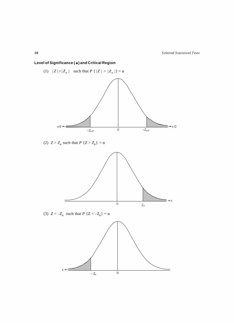
Level of Significance ( αα) and Critical Region
(1) || Z > || αZ such that P { || Z > || αZ } = α
(2) Z > Zα such that P {Z > Zα} = α
(3) Z < –Zα such that P {Z < –Zα} = α
α/2 α /20–Zα/2 –Zα/2
α0– Zα
α0 Zα
Parametric Tests 11
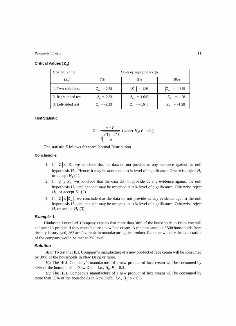
Critical Values ( Z αα)
Critical value Level of Significance (α)
(Zα) 1% 5% 10%
1. Two-sided test αZ = 2.58 αZ = 1.96 αZ = 1.645
2. Right-sided test Zα = 2.33 Zα = 1.645 Zα = 1.28
3. Left-sided test Zα = –2.33 Zα = –1.645 Zα = –1.28
Test Statistic
Z =
nPP
Pp
)1( −
− (Under H0: P = P0)
The statistic Z follows Standard Normal Distribution.
Conclusions
1. If ≤Z Zα, we conclude that the data do not provide us any evidence against the null
hypothesis H0 . Hence, it may be accepted at α% level of significance. Otherwise reject H0or accept H1 (1).
2. If ≤Z Zα, we conclude that the data do not provide us any evidence against the nullhypothesis H0 and hence it may be accepted at α% level of significance. Otherwise rejectH0 or accept H1 (2).
3. If α≤ ZZ , we conclude that the data do not provide us any evidence against the nullhypothesis H0 and hence it may be accepted at α% level of significance. Otherwise rejectH0 or accept H1 (3).
Example 1
Hindustan Lever Ltd. Company expects that more than 30% of the households in Delhi city willconsume its product if they manufacture a new face cream. A random sample of 500 households fromthe city is surveyed, 163 are favorable in manufacturing the product. Examine whether the expectationof the company would be met at 2% level.
Solution
Aim: To test the HLL Company’s manufacture of a new product of face cream will be consumedby 30% of the households in New Delhi or more.
H0: The HLL Company’s manufacture of a new product of face cream will be consumed by30% of the households in New Delhi. i.e., H0: P = 0.3.
H1: The HLL Company’s manufacture of a new product of face cream will be consumed bymore than 30% of the households in New Delhi. i.e., H1: p > 0.3
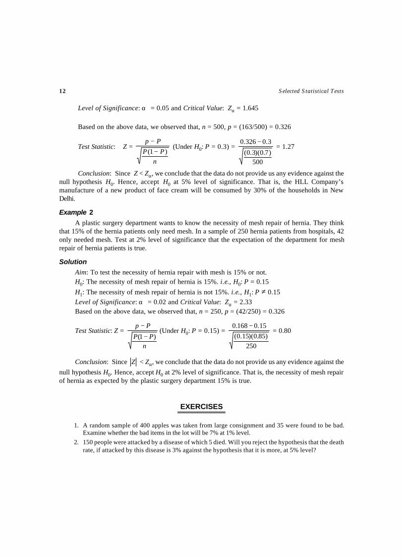
12 Selected Statistical Tests
Level of Significance: α = 0.05 and Critical Value: Zα = 1.645
Based on the above data, we observed that, n = 500, p = (163/500) = 0.326
Test Statistic: Z =
nPP
Pp
)1( −−
(Under H0: P = 0.3) =
500)7.0)(3.0(
3.0326.0 − = 1.27
Conclusion: Since Z < Zα, we conclude that the data do not provide us any evidence against thenull hypothesis H0. Hence, accept H0 at 5% level of significance. That is, the HLL Company’smanufacture of a new product of face cream will be consumed by 30% of the households in NewDelhi.
Example 2
A plastic surgery department wants to know the necessity of mesh repair of hernia. They thinkthat 15% of the hernia patients only need mesh. In a sample of 250 hernia patients from hospitals, 42only needed mesh. Test at 2% level of significance that the expectation of the department for meshrepair of hernia patients is true.
Solution
Aim: To test the necessity of hernia repair with mesh is 15% or not.H0: The necessity of mesh repair of hernia is 15%. i.e., H0: P = 0.15
H1: The necessity of mesh repair of hernia is not 15%. i.e., H1: P ≠ 0.15Level of Significance: α = 0.02 and Critical Value: Zα = 2.33Based on the above data, we observed that, n = 250, p = (42/250) = 0.326
Test Statistic: Z =
nPP
Pp
)1( −
−(Under H0: P = 0.15) =
250)85.0)(15.0(
15.0168.0 − = 0.80
Conclusion: Since Z < Zα, we conclude that the data do not provide us any evidence against the
null hypothesis H0. Hence, accept H0 at 2% level of significance. That is, the necessity of mesh repairof hernia as expected by the plastic surgery department 15% is true.
EXERCISES
1. A random sample of 400 apples was taken from large consignment and 35 were found to be bad.Examine whether the bad items in the lot will be 7% at 1% level.
2. 150 people were attacked by a disease of which 5 died. Will you reject the hypothesis that the deathrate, if attacked by this disease is 3% against the hypothesis that it is more, at 5% level?
Aim
To test the population mean µ be regarded as µ0, based on a random sample. That is, to investigate
the significance of the difference between the sample mean X and the assumed population mean µ0.
Source
Let X be the mean of a random sample of n independent observations drawn from a populationwhose mean µ is unknown and variance σ2 is known.
Assumptions
(i) The population from which, the sample drawn, is assumed as Normal distribution.
(ii) The population variance σ2 is known.
Null Hypothesis
H0: The sample has been drawn from a population with mean µ be µ0. That is, there is nosignificant difference between the sample mean X and the assumed population mean µ0. i.e., H0 : µ =µ0.
Alternative Hypotheses
H1 (1) : 0µ≠µH1 (2) : 0µ>µH1 (3) : 0µ<µ
Level of Significance ( αα) and Critical Region: (As in Test 1)
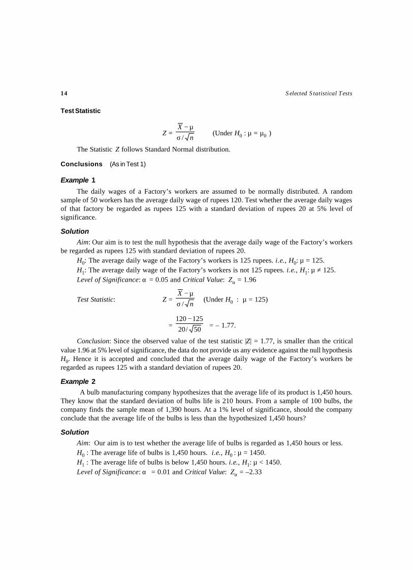
TEST – 2
TEST FOR A POPULATION MEAN(Population Variance is Known)
14 Selected Statistical Tests
Test Statistic
Z =n
X
/σµ−
(Under H0 : µ = µ0 )
The Statistic Z follows Standard Normal distribution.
Conclusions (As in Test 1)
Example 1
The daily wages of a Factory’s workers are assumed to be normally distributed. A randomsample of 50 workers has the average daily wage of rupees 120. Test whether the average daily wagesof that factory be regarded as rupees 125 with a standard deviation of rupees 20 at 5% level ofsignificance.
Solution
Aim: Our aim is to test the null hypothesis that the average daily wage of the Factory’s workersbe regarded as rupees 125 with standard deviation of rupees 20.
H0: The average daily wage of the Factory’s workers is 125 rupees. i.e., H0: µ = 125.H1: The average daily wage of the Factory’s workers is not 125 rupees. i.e., H1: µ ≠ 125.Level of Significance: α = 0.05 and Critical Value: Zα = 1.96
Test Statistic: Z =n
X
/σµ−
(Under H0 : µ = 125)
= 50/20
125120 − = – 1.77.
Conclusion: Since the observed value of the test statistic |Z| = 1.77, is smaller than the criticalvalue 1.96 at 5% level of significance, the data do not provide us any evidence against the null hypothesisH0. Hence it is accepted and concluded that the average daily wage of the Factory’s workers beregarded as rupees 125 with a standard deviation of rupees 20.
Example 2
A bulb manufacturing company hypothesizes that the average life of its product is 1,450 hours.They know that the standard deviation of bulbs life is 210 hours. From a sample of 100 bulbs, thecompany finds the sample mean of 1,390 hours. At a 1% level of significance, should the companyconclude that the average life of the bulbs is less than the hypothesized 1,450 hours?
Solution
Aim: Our aim is to test whether the average life of bulbs is regarded as 1,450 hours or less.H0 : The average life of bulbs is 1,450 hours. i.e., H0 : µ = 1450.H1 : The average life of bulbs is below 1,450 hours. i.e., H1: µ < 1450.Level of Significance: α = 0.01 and Critical Value: Zα = –2.33
Parametric Tests 15
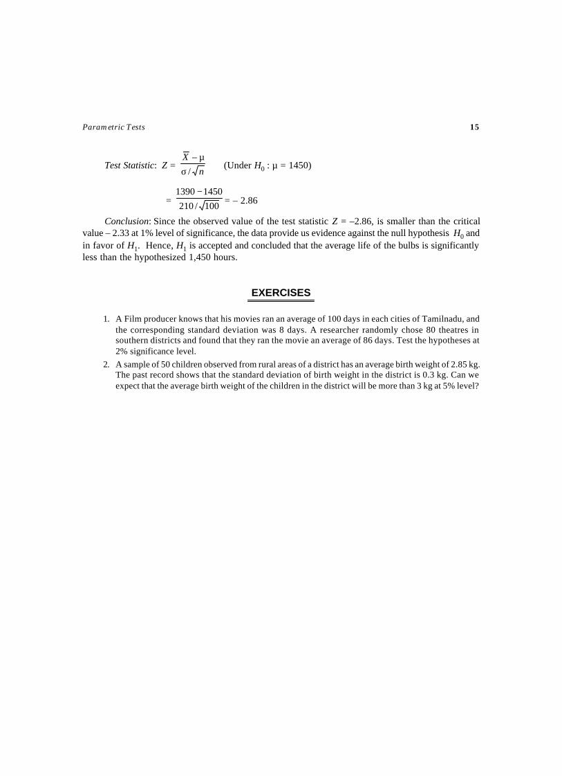
Test Statistic: Z = n
X
/
–
σµ
(Under H0 : µ = 1450)
= 100/210
14501390 −= – 2.86
Conclusion: Since the observed value of the test statistic Z = –2.86, is smaller than the criticalvalue – 2.33 at 1% level of significance, the data provide us evidence against the null hypothesis H0 andin favor of H1. Hence, H1 is accepted and concluded that the average life of the bulbs is significantlyless than the hypothesized 1,450 hours.
EXERCISES
1. A Film producer knows that his movies ran an average of 100 days in each cities of Tamilnadu, andthe corresponding standard deviation was 8 days. A researcher randomly chose 80 theatres insouthern districts and found that they ran the movie an average of 86 days. Test the hypotheses at2% significance level.
2. A sample of 50 children observed from rural areas of a district has an average birth weight of 2.85 kg.The past record shows that the standard deviation of birth weight in the district is 0.3 kg. Can weexpect that the average birth weight of the children in the district will be more than 3 kg at 5% level?
Aim
To test that the population mean µ be regarded as µ0, based on a random sample. That is, toinvestigate the significance of the difference between the sample mean X and the assumed populationm ean µ0.
Source
A random sample of n observations Xi, (i = 1, 2,…, n) be drawn from a population whose meanµ and variance σ2 are unknown.
Assumptions
(i) The population from which, the sample drawn is Normal distribution.(ii) The population variance σ2 is unknown. (Since σ2 is unknown, it is replaced by its unbiased
estimate S2 )
Null Hypothesis
H0 : The sample has been drawn from a population with mean µ be µ0. That is, there is nosignificant difference between the sample mean X and the assumed population mean µ0. i.e., H0 : µ= µ0.
Alternative Hypotheses
H1(1): µ ≠ µ0
H1(2): µ > µ0
H1(3): µ < µ0
TEST – 3
TEST FOR A POPULATION MEAN(Population Variance is Unknown)
Parametric Tests 17
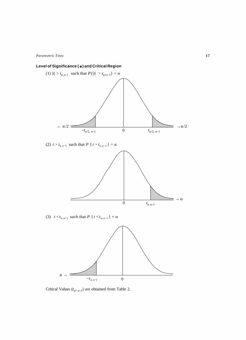
Level of Significance ( αα) and Critical Region
(1) |t| > tα,n–1 such that P{|t| > tα,n–1} = α
(2) 1, −α> ntt such that P { 1, −α> ntt } = α
(3) 1, −α< ntt such that P { 1, −α< ntt } = α
Critical Values (tα, n–1) are obtained from Table 2.
→α01, −α− nt
α→0 tα,n–1
0→α/2← α/2
–tα/2, n–1 tα/2, n–1
18 Selected Statistical Tests
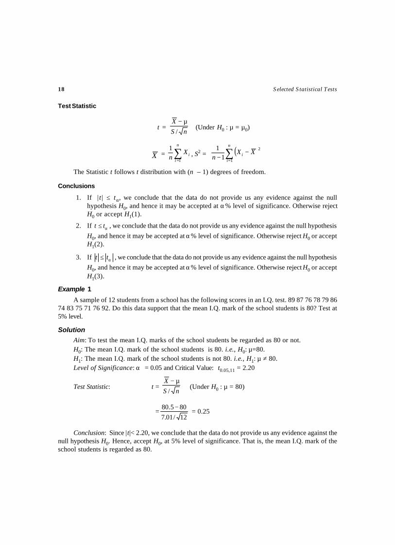
Test Statistic
t = nS
X
/
µ− (Under H0 : µ = µ0)
X = ∑=
n
iiX
n 1
1, S2 = ( )∑
=
−−
n
ii XX
n 1
2
11
The Statistic t follows t distribution with (n – 1) degrees of freedom.
Conclusions
1. If | t | ≤ tα, we conclude that the data do not provide us any evidence against the nullhypothesis H0, and hence it may be accepted at α% level of significance. Otherwise rejectH0 or accept H1(1).
2. If α≤ tt , we conclude that the data do not provide us any evidence against the null hypothesis
H0, and hence it may be accepted at α% level of significance. Otherwise reject H0 or acceptH1(2).
3. If α≤ tt , we conclude that the data do not provide us any evidence against the null hypothesis
H0, and hence it may be accepted at α% level of significance. Otherwise reject H0 or acceptH1(3).
Example 1
A sample of 12 students from a school has the following scores in an I.Q. test. 89 87 76 78 79 8674 83 75 71 76 92. Do this data support that the mean I.Q. mark of the school students is 80? Test at5% level.
Solution
Aim: To test the mean I.Q. marks of the school students be regarded as 80 or not.H0: The mean I.Q. mark of the school students is 80. i.e., H0: µ=80.H1: The mean I.Q. mark of the school students is not 80. i.e., H1: µ ≠ 80.Level of Significance: α = 0.05 and Critical Value: t0.05,11 = 2.20
Test Statistic: t = nS
X
/
µ− (Under H0 : µ = 80)
=12/01.7
805.80 − = 0.25
Conclusion: Since |t|< 2.20, we conclude that the data do not provide us any evidence against thenull hypothesis H0. Hence, accept H0, at 5% level of significance. That is, the mean I.Q. mark of theschool students is regarded as 80.
Parametric Tests 19
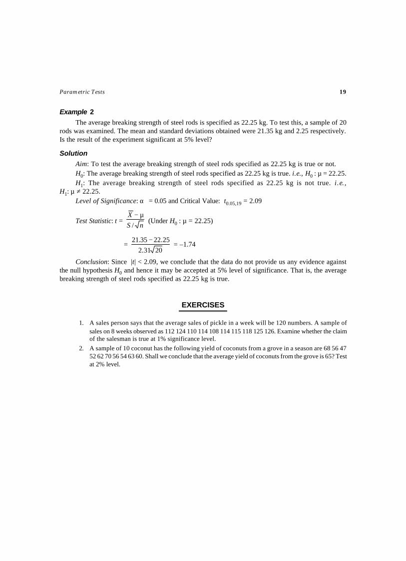
Example 2
The average breaking strength of steel rods is specified as 22.25 kg. To test this, a sample of 20rods was examined. The mean and standard deviations obtained were 21.35 kg and 2.25 respectively.Is the result of the experiment significant at 5% level?
Solution
Aim: To test the average breaking strength of steel rods specified as 22.25 kg is true or not.H0: The average breaking strength of steel rods specified as 22.25 kg is true. i.e., H0 : µ = 22.25.H1: The average breaking strength of steel rods specified as 22.25 kg is not true. i .e. ,
H1: µ ≠ 22.25.Level of Significance: α = 0.05 and Critical Value: t0.05,19 = 2.09
Test Statistic: t = nS
X
/
µ− (Under H0 : µ = 22.25)
= 2031.2
25.2235.21 − = –1.74
Conclusion: Since |t| < 2.09, we conclude that the data do not provide us any evidence againstthe null hypothesis H0 and hence it may be accepted at 5% level of significance. That is, the averagebreaking strength of steel rods specified as 22.25 kg is true.
EXERCISES
1. A sales person says that the average sales of pickle in a week will be 120 numbers. A sample ofsales on 8 weeks observed as 112 124 110 114 108 114 115 118 125 126. Examine whether the claimof the salesman is true at 1% significance level.
2. A sample of 10 coconut has the following yield of coconuts from a grove in a season are 68 56 4752 62 70 56 54 63 60. Shall we conclude that the average yield of coconuts from the grove is 65? Testat 2% level.
Aim
To test the population variance σ2 be regarded as 20σ , based on a random sample. That is, to
investigate the significance of the difference between the assumed population variance 20σ and the
sample variance s2.
Source
A random sample of n observations Xi, (i = 1, 2,…, n) be drawn from a normal population withknown mean µ and unknown variance σ2.
Assumption
The population from which, the sample drawn is normal distribution.
Null Hypothesis
H0: The population variance σ2 is 20σ . That is, there is no significant difference between the
assumed population variance 20σ and the sample variance s2. i.e., H0: σ
2 = 20σ .
Alternative Hypotheses
H1(1) : σ2 ≠ 20σ
H1(2) : σ2 > 20σ
H1(3) : σ2 < 20σ
TEST – 4
TEST FOR A POPULATION VARIANCE(Population Mean is Known)
Parametric Tests 21
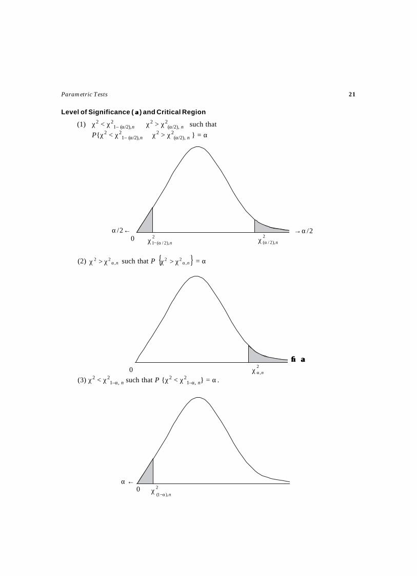
Level of Significance ( αα) and Critical Region
(1) χ2 < χ21– (α/2),n ∪ χ2 > χ2
(α/2), n such that
P{χ2 < χ21– (α/2),n ∪ χ2 > χ2
(α/2), n } = α
(2) n,22
αχ>χ such that P { }n,22
αχ>χ = α
(3) χ2 < χ21–α, n such that P {χ2 < χ2
1–α, n} = α.
0α/2← →α/2
2),2/(1 nα−χ
2),2/( nαχ
0→→ αα
2,nαχ
←α0 2
),1( nα−χ
22 Selected Statistical Tests
The critical values of Left sided test and Right sided test are provided as a and b are obtained fromTable 3.
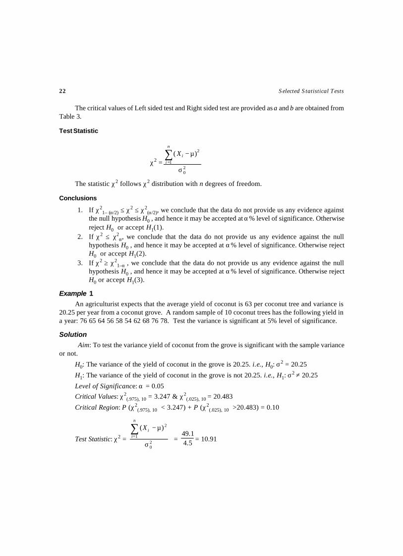
Test Statistic
χ2 =20
1
2)(
σ
µ−∑=
n
i
iX
The statistic χ2 follows χ2 distribution with n degrees of freedom.
Conclusions
1. If χ21– (α/2) ≤ χ2 ≤ χ2
(α/2), we conclude that the data do not provide us any evidence againstthe null hypothesis H0 , and hence it may be accepted at α% level of significance. Otherwisereject H0 or accept H1(1).
2. If χ2 ≤ χ2α, we conclude that the data do not provide us any evidence against the null
hypothesis H0 , and hence it may be accepted at α% level of significance. Otherwise rejectH0 or accept H1(2).
3. If χ2 ≥ χ21–α , we conclude that the data do not provide us any evidence against the null
hypothesis H0 , and hence it may be accepted at α% level of significance. Otherwise rejectH0 or accept H1(3).
Example 1
An agriculturist expects that the average yield of coconut is 63 per coconut tree and variance is20.25 per year from a coconut grove. A random sample of 10 coconut trees has the following yield ina year: 76 65 64 56 58 54 62 68 76 78. Test the variance is significant at 5% level of significance.
Solution
Aim: To test the variance yield of coconut from the grove is significant with the sample varianceor not.
H0: The variance of the yield of coconut in the grove is 20.25. i.e., H0: σ2 = 20.25
H1: The variance of the yield of coconut in the grove is not 20.25. i.e., H1: σ2 ≠ 20.25
Level of Significance: α = 0.05
Critical Values: χ2(.975), 10 = 3.247 & χ2
(.025), 10 = 20.483
Critical Region: P (χ2(.975), 10 < 3.247) + P (χ2
(.025), 10 >20.483) = 0.10
Test Statistic: χ2 = 20
1
2)(
σ
µ−∑=
n
iiX
= 5.41.49
= 10.91
Parametric Tests 23
Conclusion: Since χ21–(α/2) < χ2 < χ2
(α/2), we conclude that the data do not provide us any evidenceagainst the null hypothesis H0. Hence, H0 is accepted at 5% level of significance. That is, the varianceof the yield of coconut in the grove be regarded as 20.25.
Example 2
The variation of birth weight (as measured by the variance) of children in a region is expected tobe more than 0.16. The mean of the birth weight is known, which is 2.4 Kg. A sample of 11 childrenis selected, whose birth weight is obtained as follows.
Weight (in Kgs.): 2.7 2.5 2.6 2.6 2.7 2.5 2.5 2.3 2.4 2.3 2.5
Set up the hypotheses and for testing the expectedness at 5% level of significance.
Solution
Aim: To test the variance of the birth weight of the children be 0.16 or more.
H0: The variance of the birth weight of children in the region is 0.16. i.e., H0: σ2 = 0.16
H1: The variance of the birth weight of children in the region is more than 0.16. i.e., H1: σ2 > 0.16
Level of Significance: α = 0.05 and Critical Value: χ20.05,11 = 18.307
Test Statistic: χ2 = 20
1
2)(
σ
µ−∑=
n
iiX
= 16.031.0
= 1.94
Conclusion: Since χ2 < χ2α, we conclude that the data do not provide us any evidence against the
null hypothesis H0. Hence, H0 is accepted at 5% level of significance. That is, the variance of the birthweight of children in the region is 0.16.
EXERCISES
1. A psychologist is aware of studies showing that the mean and variability (measured as variance)of attention, spans of 5-year-olds can be summarized as 80 and 64 minutes respectively. She wantsto study whether the variability of attention span of 6-year-olds is different. A sample of 20 6-year-olds has the following attention spans in minutes: 86 89 84 78 75 74 85 71 84 71 75 68 75 71 82 85 8178 79 78. State explicit null and alternative hypotheses and test at 5% level.
2. The average and variance of daily expenditure of office going women is known as Rs.30 and Rs.10respectively. A sample of 10 office going women is selected whose daily expenditure is obtainedas 35 33 40 30 25 28 35 28 35 40. Test whether the variance of the daily expenditure of office goingwomen is 10 at 1% level of significance.
Aim
To test the population variance σ2 be regarded as 20σ , based on a random sample. That is, to
investigate the significance of the difference between the assumed population variance 20σ and the
sample variance s2.
Source
A random sample of n observations Xi, (i = 1, 2,…, n) be drawn from a normal population withmean µ and variance σ2 (both are unknown). The unknown population mean µ is estimated by its
unbiased estimate X .
Assumption
The population from which, the sample drawn is normal distribution.
Null Hypothesis
H0: The population variance σ2 is 20σ . That is, there is no significant difference between the
assumed population variance 20σ and the sample variance s2. i.e., H0: σ
2 = 20σ .
Alternative Hypotheses
H1(1) : σ2 ≠ σ02
H1(2) : σ2 > σ02
H1(3) : σ2 < σ02
Level of Significance ( αα) and Critical Region: (As in Test 4)
TEST – 5
TEST FOR A POPULATION VARIANCE(Population Mean is Unknown)
Parametric Tests 25
Test Statistic
χ2 = 20
1
2)(
σ
−∑=
n
ii XX
The statistic χ2 follows χ2 distribution with (n–1) degrees of freedom.
Conclusions (As in Test 4)
Example 1
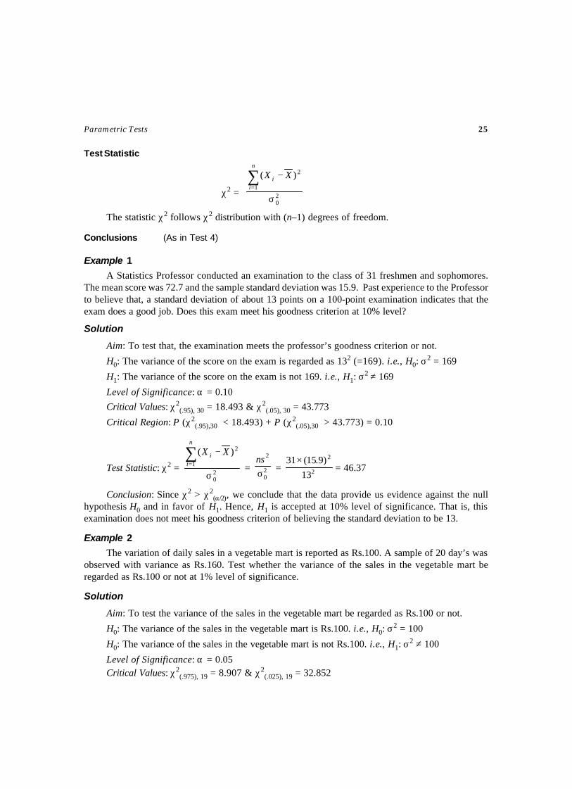
A Statistics Professor conducted an examination to the class of 31 freshmen and sophomores.The mean score was 72.7 and the sample standard deviation was 15.9. Past experience to the Professorto believe that, a standard deviation of about 13 points on a 100-point examination indicates that theexam does a good job. Does this exam meet his goodness criterion at 10% level?
Solution
Aim: To test that, the examination meets the professor’s goodness criterion or not.
H0: The variance of the score on the exam is regarded as 132 (=169). i.e., H0: σ2 = 169
H1: The variance of the score on the exam is not 169. i.e., H1: σ2 ≠ 169
Level of Significance: α = 0.10
Critical Values: χ2(.95), 30 = 18.493 & χ2
(.05), 30 = 43.773
Critical Region: P (χ2(.95),30 < 18.493) + P (χ2
(.05),30 > 43.773) = 0.10
Test Statistic: χ2 = 20
1
2)(
σ
−∑=
n
ii XX
= 20
2
σns
= 2
2
13
)9.15(31×= 46.37
Conclusion: Since χ2 > χ2(α/2), we conclude that the data provide us evidence against the null
hypothesis H0 and in favor of H1. Hence, H1 is accepted at 10% level of significance. That is, thisexamination does not meet his goodness criterion of believing the standard deviation to be 13.
Example 2
The variation of daily sales in a vegetable mart is reported as Rs.100. A sample of 20 day’s wasobserved with variance as Rs.160. Test whether the variance of the sales in the vegetable mart beregarded as Rs.100 or not at 1% level of significance.
Solution
Aim: To test the variance of the sales in the vegetable mart be regarded as Rs.100 or not.
H0: The variance of the sales in the vegetable mart is Rs.100. i.e., H0: σ2 = 100
H0: The variance of the sales in the vegetable mart is not Rs.100. i.e., H1: σ2 ≠ 100
Level of Significance: α = 0.05Critical Values: χ2
(.975), 19 = 8.907 & χ2(.025), 19 = 32.852
26 Selected Statistical Tests
Critical Region: P (χ2(.975), 19 < 8.907) + P (χ2
(.025), 19 > 32.852) = 0.05
Test Statistic: χ2 = 20
1
2)(
σ
−∑=
n
ii XX
= 1003200
= 32
Conclusion: Since χ21–(α/2) < χ2 < χ2
(α/2), we conclude that the data do not provide us any evidenceagainst the null hypothesis H0 . Hence, H0 is accepted at 5% level of significance. That is, the varianceof the sales in the vegetable mart is Rs.100.
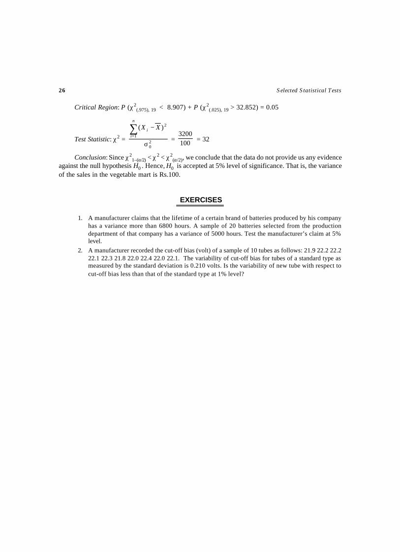
EXERCISES
1. A manufacturer claims that the lifetime of a certain brand of batteries produced by his companyhas a variance more than 6800 hours. A sample of 20 batteries selected from the productiondepartment of that company has a variance of 5000 hours. Test the manufacturer’s claim at 5%level.
2. A manufacturer recorded the cut-off bias (volt) of a sample of 10 tubes as follows: 21.9 22.2 22.222.1 22.3 21.8 22.0 22.4 22.0 22.1. The variability of cut-off bias for tubes of a standard type asmeasured by the standard deviation is 0.210 volts. Is the variability of new tube with respect tocut-off bias less than that of the standard type at 1% level?
Aim
To test that, the observed frequencies are good for fit with the theoretical frequencies. That is, toinvestigate the significance of the difference between the observed frequencies and the expectedfrequencies, arranged in K classes.
Source
Let Oi, (i = 1, 2,…, K) is a set of observed frequencies on K classes based on any experiment andEi (i = 1, 2,…, K) is the corresponding set of expected (theoretical or hypothetical) frequencies.
Assumptions
(i) The observed frequencies in the K classes should be independent.
(ii) ∑∑==
=K
ii
K
ii EO
11
= N.
(iii) The total frequency, N should be sufficiently large (i.e., N > 50).(iv) Each expected frequency in the K classes should be at least 5.
Null Hypothesis
H0: The observed frequencies are good for fit with the theoretical frequencies. That is, there isno significant difference between the observed frequencies and the expected frequencies, arranged inK classes.
Alternative Hypothesis
H1: The observed frequencies are not good for fit with the theoretical frequencies. That is, thereis a significant difference between the observed frequencies and the expected frequencies, arranged inK classes.
TEST FOR GOODNESS OF FIT
TEST – 6
28 Selected Statistical Tests
Level of Significance ( αα) and Critical Region
χ2 > χ2α,(K–1) such that P{χ2 > χ2
α,(K–1)} = α
Test Statistic
χ2 =
2
1∑
=
−K
i i
ii
EEO
The Statistic χ2 follows χ2 distribution with (K–1) degrees of freedom.
Conclusion
If χ2 ≤ χ2α,(K–1), we conclude that the data do not provide us any evidence against the null
hypothesis H0 and hence it may be accepted at α% level of significance. Otherwise reject H0 or acceptH1.
Example 1
The sales of milk from a milk booth are varying from day-to-day. A sample of one-week sales(Number of Liters) is observed as follows.
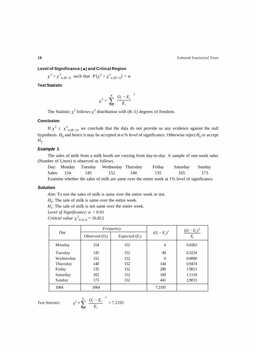
Day: Monday Tuesday Wednesday Thursday Friday Saturday SundaySales: 154 145 152 140 135 165 173Examine whether the sales of milk are same over the entire week at 1% level of significance.
Solution
Aim: To test the sales of milk is same over the entire week or not.H0: The sale of milk is same over the entire week.H1: The sale of milk is not same over the entire week.Level of Significance: α = 0.01Critical value: χ2
0.01,6 = 16.812
Frequency
Observed (Oi) Expected (Ei)
Monday 154 152 4 0.0263
Tuesday 145 152 49 0.3224Wednesday 152 152 0 0.0000Thursday 140 152 144 0.9474Friday 135 152 289 1.9013Saturday 165 152 169 1.1118Sunday 173 152 441 2.9013
1064 1064 7.2105
Test Statistic: χ2 =2
1∑
=
−K
i i
ii
EEO
= 7.2105
i
ii
EEO 2)( −2)( ii EO −Day
Parametric Tests 29
Conclusion: Since χ2 < χ2α,(K–1), we conclude that the data do not provide us any evidence
against the null hypothesis H0 . Hence, H0 is accepted at 1% level of significance. That is, the sales ofmilk are same over the entire week.
Example 2
In an experiment on pea breeding, Mendal obtained the following frequencies of seeds from 560seeds: 312 rounded and yellow (RY), 104 wrinkled and yellow (WY); 112 round and green (RG), 32wrinkled and green (WG). Theory predicts that the frequencies should be in the proportion 9:3:3:1respectively. Set up the hypothesis and test it for 1% level.
Solution
Aim: To test the observed frequencies of the pea breeding in the ratio 9:3:3:1.
H0: The observed frequencies of the pea breeding are in the ratio 9:3:3:1.
H1: The observed frequencies of the pea breeding are not in the ratio 9:3:3:1.
Level of Significance: α = 0.01
Critical value: χ20.01,3 = 11.345
Seed type Frequencyi
ii
EEO 2)( −
Observed (Oi) Expected (Ei)2)( ii EO −
RY 312 315 9 0.0286WY 104 105 1 0.0095RG 112 105 49 0.4667WG 32 35 9 0.2571
560 560 0.7619
Test Statistic: χ2 =
2
1∑
=
−K
i i
ii
EEO
= 0.7619
Conclusion: Since χ2 < χ2α,(K–1) , we conclude that the data do not provide us any evidence
against the null hypothesis H0 . Hence, H0 is accepted at 1% level of significance. That is, the observedfrequencies of the pea breeding are in the ratio 9:3:3:1.
EXERCISES
1. A chemical extract plant processes seawater to collect sodium chloride and magnesium. It isknown that seawater contains sodium chloride, magnesium and other elements in the ratio of62:4:34. A sample of 300 hundred tones of seawater has resulted in 195 tones of sodium chlorideand 9 tones of magnesium. Are these data consistent with the known composition of seawater at10% level?
2. Among 80 off springs of a certain cross between guinea pigs, 42 were red, 16 were black and 22were white. According to genetic model, these numbers should be in the ratio 9:3:4. Are theseconsistent with the model at 1% level of significance?
Aim
To test the two population proportions P1 and P2 be equal, based on two random samples. Thatis, to investigate the significance of the difference between the two sample proportions p1 and p2.
Source
From a random sample of n1 observations, X1 observations possessing an attribute A whosesample proportion p1 is X1/n1. Let the corresponding proportion in the population be denoted by P1,which is unknown. From another sample of n2 observations, X2 observations possessing the attributeA whose sample proportion p2 is X2/n2. Let the corresponding proportion in the population be denotedby P2, which is unknown.
Assumption
The sample sizes of the two samples are sufficiently large (i.e., n1, n2 ≥ 30 ) to justify the normalapproximation to the binomial.
Null Hypothesis
H0: The two population proportions P1 and P2 are equal. That is, there is no significant differencebetween the two sample proportions p1 and p2. i.e., H0: P1 = P2.
Alternative Hypotheses
H1(1) : P1 ≠ P2
H1(2) : P1 > P2
H1(3) : P1 < P2
Level of Significance ( αα) and Critical Region: (As in Test 1)
TEST FOR EQUALITY OF TWO
POPULATION PROPORTIONS
TEST – 7
Parametric Tests 31
Test Statistic
Z =
+−
−−−
∧∧
21
2121
11)1(
)()(
nnPP
PPpp(Under H0: P1 = P2)
∧P =
21
2211
nn
pnpn
++
The statistic Z follows Standard Normal distribution.
Conclusions (As in Test 1)
Example 1
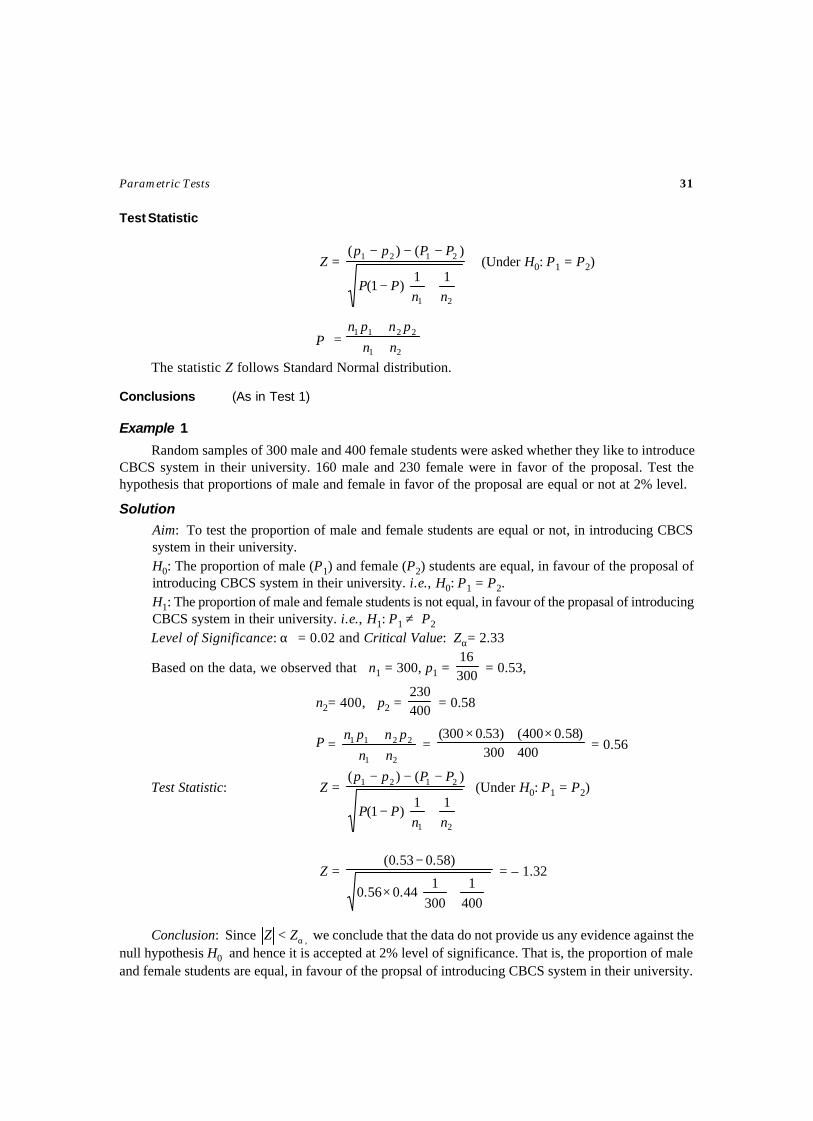
Random samples of 300 male and 400 female students were asked whether they like to introduceCBCS system in their university. 160 male and 230 female were in favor of the proposal. Test thehypothesis that proportions of male and female in favor of the proposal are equal or not at 2% level.
Solution
Aim: To test the proportion of male and female students are equal or not, in introducing CBCSsystem in their university.H0: The proportion of male (P1) and female (P2) students are equal, in favour of the proposal ofintroducing CBCS system in their university. i.e., H0: P1 = P2.H1: The proportion of male and female students is not equal, in favour of the propasal of introducingCBCS system in their university. i.e., H1: P1 ≠ P2
Level of Significance: α = 0.02 and Critical Value: Zα= 2.33
Based on the data, we observed that n1 = 300, p1 = 30016
= 0.53,
n2= 400, p2 = 400230
= 0.58
∧P =
21
2211
nn
pnpn
++
= 400300)58.0400()53.0300(
+×+×
= 0.56
Test Statistic: Z =
+−
−−−
∧∧
21
2121
11)1(
)()(
nnPP
PPpp (Under H0: P1 = P2)
Z =
+×
−
4001
3001
44.056.0
)58.053.0( = – 1.32
Conclusion: Since ,α< ZZ we conclude that the data do not provide us any evidence against thenull hypothesis H0 and hence it is accepted at 2% level of significance. That is, the proportion of maleand female students are equal, in favour of the propsal of introducing CBCS system in their university.
32 Selected Statistical Tests
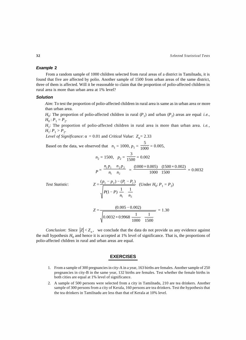
Example 2
From a random sample of 1000 children selected from rural areas of a district in Tamilnadu, it isfound that five are affected by polio. Another sample of 1500 from urban areas of the same district,three of them is affected. Will it be reasonable to claim that the proportion of polio-affected children inrural area is more than urban area at 1% level?
Solution
Aim: To test the proportion of polio-affected children in rural area is same as in urban area or morethan urban area.H0: The proportion of polio-affected children in rural (P1) and urban (P2) areas are equal i.e.,H0 : P1 = P2.H1: The proportion of polio-affected children in rural area is more than urban area. i.e. ,H1: P1 > P2.Level of Significance: α = 0.01 and Critical Value: Zα= 2.33
Based on the data, we observed that n1 = 1000, p1 = 10005
= 0.005,
n2 = 1500, p2 = 15003
= 0.002
∧P =
21
2211
nn
pnpn
++
= 15001000)002.01500()005.01000(
+×+×
= 0.0032
Test Statistic: Z =
+−
−−−
∧∧
21
2121
11)1(
)()(
nnPP
PPpp (Under H0: P1 = P2)
Z =
+×
−
15001
10001
9968.00032.0
)002.0005.0( = 1.30
Conclusion: Since ,α< ZZ we conclude that the data do not provide us any evidence againstthe null hypothesis H0 and hence it is accepted at 1% level of significance. That is, the proportions ofpolio-affected children in rural and urban areas are equal.
EXERCISES
1. From a sample of 300 pregnancies in city-A in a year, 163 births are females. Another sample of 250pregnancies in city-B in the same year, 132 births are females. Test whether the female births inboth cities are equal at 1% level of significance.
2. A sample of 500 persons were selected from a city in Tamilnadu, 210 are tea drinkers. Anothersample of 300 persons from a city of Kerala, 160 persons are tea drinkers. Test the hypothesis thatthe tea drinkers in Tamilnadu are less than that of Kerala at 10% level.
Aim
To test the two population means are equal, based on two random samples. That is, to investigatethe significance of the difference between the two sample means 1X and 2X .
Source
A random sample of n1 observations has the mean 1X be drawn from a population with unknown
mean µ1. A random sample of n2 observations has the mean 2X be drawn from another populationwith unknown mean µ2.
Assumptions
(i) The populations, from which, the two samples drawn are assumed as Normal distributions.(ii) The two Population variances are equal and known which is denoted by σ2.
Null Hypothesis
H0: The two population means µ1 and µ2 are equal. That is, there is no significant difference
between the two sample means 1X and 2X .
i.e., H0: µ1 = µ2
Alternative Hypotheses
H1(1) : µ1 ≠ µ2
H1(2) : µ1 > µ2
H1(3) : µ1 < µ2
Level of Significance ( αα) and Critical Region: (As in Test 1)
TEST FOR EQUALITY OF TWOPOPULATION MEANS
(Population Variances are Equal and Known)
TEST – 8
34 Selected Statistical Tests
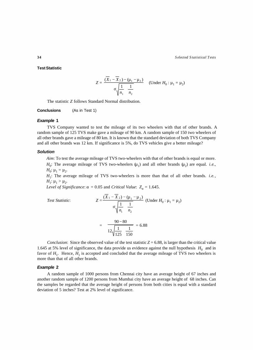
Test Statistic
Z =
21
2121
11
)()(
nn
XX
+σ
µ−µ−−(Under H0 : µ1 = µ2)
The statistic Z follows Standard Normal distribution.
Conclusions (As in Test 1)
Example 1
TVS Company wanted to test the mileage of its two wheelers with that of other brands. Arandom sample of 125 TVS make gave a mileage of 90 km. A random sample of 150 two wheelers ofall other brands gave a mileage of 80 km. It is known that the standard deviation of both TVS Companyand all other brands was 12 km. If significance is 5%, do TVS vehicles give a better mileage?
Solution
Aim: To test the average mileage of TVS two-wheelers with that of other brands is equal or more.H0: The average mileage of TVS two-wheelers (µ1) and all other brands (µ2) are equal. i.e.,H0: µ1 = µ2.H1: The average mileage of TVS two-wheelers is more than that of all other brands. i.e. ,H1: µ1 > µ2.Level of Significance: α = 0.05 and Critical Value: Zα = 1.645.
Test Statistic: Z =
21
2121
11
)()(
nn
XX
+σ
µ−µ−− (Under H0 : µ1 = µ2)
=
1501
125112
8090
+
− = 6.88
Conclusion: Since the observed value of the test statistic Z = 6.88, is larger than the critical value1.645 at 5% level of significance, the data provide us evidence against the null hypothesis H0 and infavor of H1. Hence, H1 is accepted and concluded that the average mileage of TVS two wheelers ismore than that of all other brands.
Example 2
A random sample of 1000 persons from Chennai city have an average height of 67 inches andanother random sample of 1200 persons from Mumbai city have an average height of 68 inches. Canthe samples be regarded that the average height of persons from both cities is equal with a standarddeviation of 5 inches? Test at 2% level of significance.
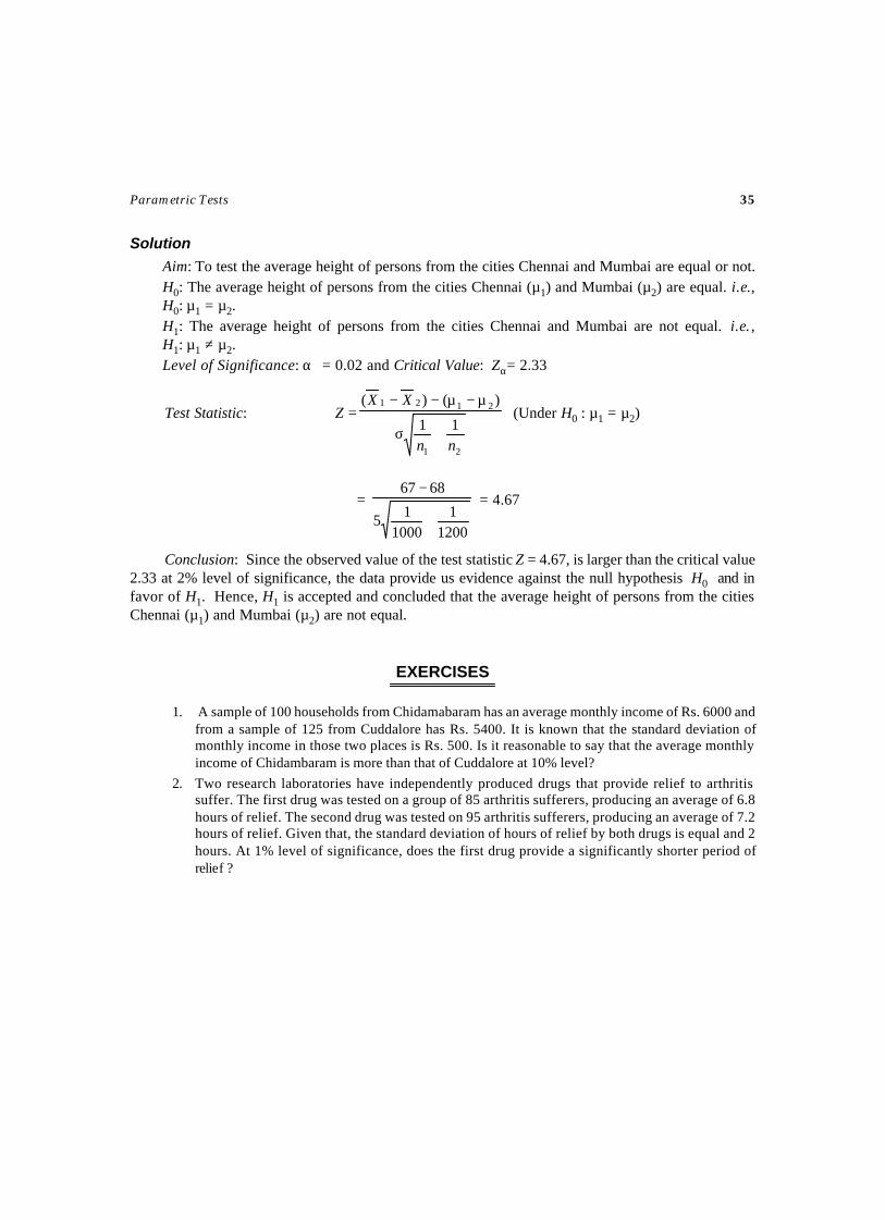
Parametric Tests 35
Solution
Aim: To test the average height of persons from the cities Chennai and Mumbai are equal or not.H0: The average height of persons from the cities Chennai (µ1) and Mumbai (µ2) are equal. i.e.,H0: µ1 = µ2.H1: The average height of persons from the cities Chennai and Mumbai are not equal. i.e. ,H1: µ1 ≠ µ2.Level of Significance: α = 0.02 and Critical Value: Zα= 2.33
Test Statistic: Z =
21
2121
11
)()(
nn
XX
+σ
µ−µ−− (Under H0 : µ1 = µ2)
=
12001
100015
6867
+
− = 4.67
Conclusion: Since the observed value of the test statistic Z = 4.67, is larger than the critical value2.33 at 2% level of significance, the data provide us evidence against the null hypothesis H0 and infavor of H1. Hence, H1 is accepted and concluded that the average height of persons from the citiesChennai (µ1) and Mumbai (µ2) are not equal.
EXERCISES
1. A sample of 100 households from Chidamabaram has an average monthly income of Rs. 6000 andfrom a sample of 125 from Cuddalore has Rs. 5400. It is known that the standard deviation ofmonthly income in those two places is Rs. 500. Is it reasonable to say that the average monthlyincome of Chidambaram is more than that of Cuddalore at 10% level?
2. Two research laboratories have independently produced drugs that provide relief to arthritissuffer. The first drug was tested on a group of 85 arthritis sufferers, producing an average of 6.8hours of relief. The second drug was tested on 95 arthritis sufferers, producing an average of 7.2hours of relief. Given that, the standard deviation of hours of relief by both drugs is equal and 2hours. At 1% level of significance, does the first drug provide a significantly shorter period ofrelief ?
Aim
To test the two population means be equal, based on two random samples. That is, to investigatethe significance of the difference between the two sample means 1X and 2X is significant.
Source
A random sample of n1 observations has the mean 1X be drawn from a population with unknown
mean µ1 and known variance 21σ . A random sample of n2 observations has the mean 2X be drawn
from another population with unknown mean µ2 and known variance 22σ .
Assumptions
(i) The populations from which, the two samples drawn, are Normal distributions.
(ii) The population variances 21σ and
22σ are known.
Null Hypothesis
H0: The two population means µ1 and µ2 are equal. That is, there is no significant differencebetween the two sample means 1X and 2X .
i.e., H0 : µ1 = µ2
Alternative Hypotheses
H1(1) : µ1 ≠ µ2
H1(2) : µ1 > µ2
H1(3) : µ1 < µ2
Level of Significance ( αα) and Critical Region: (As in Test 1)
TEST FOR EQUALITY OF TWOPOPULATION MEANS
(Population Variances are Unequal and Known)
TEST – 9
Parametric Tests 37
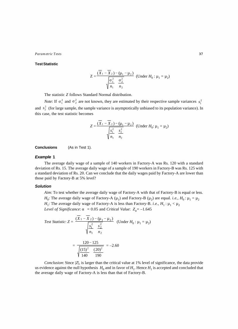
Test Statistic
Z =
2
22
1
21
2121 )()(
nn
XX
σ+
σ
µ−µ−− (Under H0 : µ1 = µ2)
The statistic Z follows Standard Normal distribution.
Note: If 21σ and 2
2σ are not known, they are estimated by their respective sample variances 21s
and 22s (for large sample, the sample variance is asymptotically unbiased to its population variance). In
this case, the test statistic becomes
Z =
2
22
1
21
2121 )()(
n
s
n
s
XX
+
µ−µ−− (Under H0: µ1 = µ2)
Conclusions (As in Test 1).
Example 1
The average daily wage of a sample of 140 workers in Factory-A was Rs. 120 with a standarddeviation of Rs. 15. The average daily wage of a sample of 190 workers in Factory-B was Rs. 125 witha standard deviation of Rs. 20. Can we conclude that the daily wages paid by Factory-A are lower thanthose paid by Factory-B at 5% level?
Solution
Aim: To test whether the average daily wage of Factory-A with that of Factory-B is equal or less.H0: The average daily wage of Factory-A (µ1) and Factory-B (µ2) are equal. i.e., H0 : µ1 = µ2
H1: The average daily wage of Factory-A is less than Factory-B. i.e., H1 : µ1 < µ2
Level of Significance: α = 0.05 and Critical Value: Zα= –1.645
Test Statistic: Z =
2
22
1
21
2121 )()(
ns
ns
XX
+
µ−µ−− (Under H0 : µ1 = µ2)
=
190)20(
140)15(
12512022
+
− = –2.60
Conclusion: Since |Z|, is larger than the critical value at 1% level of significance, the data provideus evidence against the null hypothesis H0 and in favor of H1. Hence H1 is accepted and concluded thatthe average daily wage of Factory-A is less than that of Factory-B.
38 Selected Statistical Tests
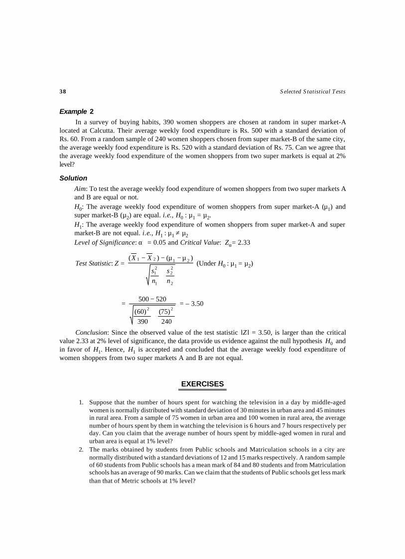
Example 2
In a survey of buying habits, 390 women shoppers are chosen at random in super market-Alocated at Calcutta. Their average weekly food expenditure is Rs. 500 with a standard deviation ofRs. 60. From a random sample of 240 women shoppers chosen from super market-B of the same city,the average weekly food expenditure is Rs. 520 with a standard deviation of Rs. 75. Can we agree thatthe average weekly food expenditure of the women shoppers from two super markets is equal at 2%level?
Solution
Aim: To test the average weekly food expenditure of women shoppers from two super markets Aand B are equal or not.H0: The average weekly food expenditure of women shoppers from super market-A (µ1) andsuper market-B (µ2) are equal. i.e., H0 : µ1 = µ2.H1: The average weekly food expenditure of women shoppers from super market-A and supermarket-B are not equal. i.e., H1 : µ1 ≠ µ2
Level of Significance: α = 0.05 and Critical Value: Zα= 2.33
Test Statistic: Z =
2
22
1
21
2121 )()(
ns
ns
XX
+
µ−µ−− (Under H0 : µ1 = µ2)
=
240)75(
390)60(
52050022
+
− = – 3.50
Conclusion: Since the observed value of the test statistic lZ l = 3.50, is larger than the criticalvalue 2.33 at 2% level of significance, the data provide us evidence against the null hypothesis H0 andin favor of H1. Hence, H1 is accepted and concluded that the average weekly food expenditure ofwomen shoppers from two super markets A and B are not equal.
EXERCISES
1. Suppose that the number of hours spent for watching the television in a day by middle-agedwomen is normally distributed with standard deviation of 30 minutes in urban area and 45 minutesin rural area. From a sample of 75 women in urban area and 100 women in rural area, the averagenumber of hours spent by them in watching the television is 6 hours and 7 hours respectively perday. Can you claim that the average number of hours spent by middle-aged women in rural andurban area is equal at 1% level?
2. The marks obtained by students from Public schools and Matriculation schools in a city arenormally distributed with a standard deviations of 12 and 15 marks respectively. A random sampleof 60 students from Public schools has a mean mark of 84 and 80 students and from Matriculationschools has an average of 90 marks. Can we claim that the students of Public schools get less markthan that of Metric schools at 1% level?
Aim
To test the null hypothesis of the mean of the two populations are equal, based on two randomsamples. That is, to investigate the significance of the difference between the two sample means 1Xand 2X .
Source
A random sample of n1 observations X1i, (i = 1, 2,…, n1) be drawn from a population withunknown mean µ1 . A random sample of n2 observations X2j, (j = 1, 2,…, n2) be drawn from anotherpopulation with unknown mean µ2.
Assumptions
(i) The populations from which, the two samples drawn, are Normal distributions.(ii) The two Population variances are equal and unknown which is denoted by σ2 (Since σ2 is
unknown, it is replace by unbiased estimate S2 ).
Null Hypothesis
H0: The two population means µ1 and µ2 are equal. That is, there is no significant differencebetween the two sample means 1X and 2X .
i.e., H0: µ1 = µ2
Alternative Hypotheses
H1(1) : µ1 ≠ µ2
H1(2) : µ1 > µ2
H1(3) : µ1 < µ2
Level of Significance ( αα) and Critical Region
1. )2–21(,|| nntt +α< such that P { )2–21(,|| nntt +α> } = α
TEST FOR EQUALITY OF TWO
POPULATION MEANS(Population Variances are Equal and Unknown)
TEST – 10
40 Selected Statistical Tests
2. )2–(, 21 nntt +α> such that P { )2–(, 21 nntt +α> } = α
3. )2–(, 21– nntt +α< such that P { )2–(, 21
– nntt +α< } = α
Critical Values )( )2–(, 21 nnt +α are obtained from Table 2.
Test Statistic
t =
21
2121
11
)()(
nnS
XX
+
µ−µ−− (Under H0 : µ1 = µ2)
1X = ∑=
1
11
1
1 n
iiX
n, 2X = ∑
=
2
12
2
1 n
jiX
n and 2S =
( ) ( )221
1 12211
1 2
−+
−+−∑ ∑= =
nn
XXXXn
i
n
jii
.
The statistic t follows t distribution with (n1 + n2 – 2 ) degrees of freedom.
Conclusions (As in Test 3)
Example 1
The gain in weight of two random samples of chicks on two different diets A and B are givenbelow. Examine whether the difference in mean increases in weight is significant.
Diet A: 2.5 2.25 2.35 2.60 2.10 2.45 2.5 2.1 2.2Diet B: 2.45 2.50 2.60 2.77 2.60 2.55 2.65 2.75 2.45 2.50
Solution
Aim: To test the mean increases in weights by diet-A (µ1) and diet-B (µ2) are equal or not.H0 : The mean increases in weights by both diets are equal. i.e., H0 : µ1 = µ2
H1 : The mean increases in weights by both diets are not equal. i.e., H1 : µ1 ≠ µ2
Level of significance: α = 0.05(say) and Critical value: t0.05 for 17 d.f = 2.11
Test Statistic: t =
21
2121
11
)()(
nnS
XX
+
µ−µ−− (Under H0 : µ1 = µ2)
=
101
9116.0
)58.234.2(
+
− = –2.25
Conclusion: Since | t | > tα, we conclude that the data provide us evidence against the nullhypothesis H0 and in favor of H1. Hence, H1 is accepted at 5% level of significance. That is, the meanincrease in weights by two diets A and B are not equal.
Parametric Tests 41
Example 2
A researcher is interested to know whether the performance in a public examination by studentsof schools from Tsunami affected area compared with other students is poor or not. A random sampleof 10 students from coastal area schools is selected whose marks are given below. 68 72 64 65 56 7264 56 60 73. Another sample of 8 students from non-coastal area schools has the following marks 7678 68 72 83 85 88 78. Test at 1% level of the hypothesis.
Solution
Aim: To test the performance in a public examination by students of schools from Tsunamiaffected area compared with other students is equal or less.H0: The performance in a public examination by students of schools from Tsunami affected area(µ1) compared with other students (µ2) is equal. i.e., H0: µ1 = µ2
H1: The performance in a public examination by students of schools from Tsunami affected areais less than that of other students. i.e., H1: µ1 < µ2
Level of Significance: α = 0.01 and Critical value: t0.01 for 16 d.f = – 2.58
Test Statistic: t =
21
2121
11
)()(
nnS
XX
+
µ−µ−− (Under H0 : µ1 = µ2)
=
81
10188.6
)5.7865(
+
−= – 4.13
Conclusion: Since | t | > |tα|, we conclude that the data provide us evidence against the nullhypothesis H0 and in favor of H1. Hence, H1 is accepted at 1% level of significance. That is, theperformance in a public examination by students of schools from Tsunami affected area is less thanthat of other students.
EXERCISES
1. A paper company produces covers on two machines whose data is given below. The averagenumber of items produced by two machines per hour is 250 and 280 with standard deviations 16and 20 respectively based on records of 50 hours production. Can we expect that the two machinesare equally efficient at 10% level of significance?
2. The yield of two varieties of brinjal on two independent sample of 10 and 12 plants are givenbelow. Test whether the yield of Variety-A is more than Variety-B at 2% level of significance.Variety-A: 18 15 16 20 22 20 23 18 20 25Variety-B: 12 14 16 13 16 20 22 24
Aim
To test the treatment applied is effective or not, based on a random sample. That is, to investigatethe significance of the difference between before and after the treatment in the sample.
Source
Let Xi, (i = 1, 2,…, n) be the observations made initially from n individuals as a random sample ofsize n. A treatment is applied to the above individuals and observations are made after the treatment andare denoted by Yi, (i = 1, 2,…, n). That is, (Xi, Yi) denotes the pair of observations obtained from theith individual, before and after the treatment applied. Let µX is unknown population mean before thetreatment and µY is the unknown population mean after the treatment.
Assumptions
(i) The observations for the two samples must be obtained in pair.(ii) The population from which, the sample drawn is normal.
Null Hypothesis
H0: The treatment applied, is ineffective. That is, there is no significant difference between beforeand after the treatment applied.
i.e., H0: µd = µX – µY = 0.
Alternative Hypotheses
H1(1) : µd ≠ 0H1(2) : µd > 0H1(3) : µd < 0
Level of Significance ( αα) and Critical Region: (As in Test 3)
TEST FOR PAIRED OBSERVATIONS
TEST – 11
Parametric Tests 43
Test Statistic
t =nS
d
d
d
/
µ− ( Under H0 : µd = 0)
d = n
dn
ii∑
=1, id = ii YX − , 2
dS = ( )2
111 ∑
=
−−
n
ii dd
n
The statistic t follows t distribution with (n–1) degrees of freedom.
Conclusions (As in Test 3)
Example 1
A health spa has advertised a weight-reducing program and has claimed that the average participantin the program loses more than 5 kgs. A random sample of 10 participants has the following weightsbefore and after the program. Test his claim at 5% level of significance.
Solution
Weights before: 80 78 75 86 90 87 95 78 86 90Weights after: 76 75 70 80 84 83 91 72 83 83Aim: To test the claim of health spa on average weight reduction is five kgs or more.H0: The average weight reduction is only 5 kgs. i.e., H0: µd = µx – µy = 5H1: The average weight reduction is more than 5 kgs. i.e., H1: µd > 5.Level of Significance: α = 0.05 and Critical value: t0.05,9 = 1.83
Test Statistic: t =nS
d
d
d
/
µ− (Under H0: µd = 0)
=10/41.1
7.4 =10.54
Conclusion: Since t > tα, we conclude that the data provide us evidence against the null hypothesisH0 and in favor of H1. Hence, H1 is accepted at 5% level of significance. That is, the average weightreduction is more than 5 kgs.
Example 2
A manufacturer claims that a significant gain on weight will be attained for infants if a newvariety of health drink marketed by him. A sample of 10 babies was selected and was given the abovediet for a month and the weights were observed before (A) and after (B) the diet given. Examinewhether the claim of the manufacturer is true at 2% level of significance.
A : 3.50 3.75 3.65 4.10 3.65 3.55 3.60 4.20 3.80 3.50B : 3.80 4.20 3.90 4.50 3.75 4.20 3.60 4.35 4.20 3.40
44 Selected Statistical Tests
Solution
Aim: To test the claim of manufacturer on marketing a new variety of health drink, that willpromote weight gain or not.H0: The claim of manufacturer on marketing a new variety of health drink that will promoteweight gain is not true. i.e., H0: µd = 0.H1: The claim of manufacturer on marketing a new variety of health drink that will promoteweight gain is true. i.e., H1: µd ≠ 0.Level of Significance: α = 0.02 and Critical value: t0.02,9 = 2.82
Test Statistic: t =nS
d
d
d
/
µ− (Under H0: µd = 0)
=10/24.0
26.0− = –3.43
Conclusion: Since |t| > tα, we conclude that the data provide us evidence against the nullhypothesis H0 and in favor of H1. Hence, H1 is accepted at 2% level of significance. That is, the claimof manufacturer on marketing a new variety of health drink that will promote weight gain is true.
EXERCISES
1. The following data shows the additional hours of sleep gained by 15 patients in an experiment totest the effect of a drug. Do these data shows the evidence that the drug produces additionalhours of sleep at 2% level?Hours gained : 2.5 3.0 2.25 3.25 1.75 1.5 2.5 2.25 3.0 3.25 3.0 2.5 2.75 3.25 3.75.
2. A coaching centre for giving coach to civil service examination claims that there will be a significantimprovement in obtainning scores to the students. A random sample of 12 students was selected.They are conducted examinations, before and after the coach, and are given below. Test whetherthe claim of the coaching centre at 1% level of significance.
Student: 1 2 3 4 5 6 7 8 9 10 11 12
Score Before Coaching : 68 72 74 67 79 78 82 78 77 77 80 78Score After Coaching : 78 75 78 80 80 85 80 75 90 92 95 90
Aim
To test the standard deviations of the two populations σ1 and σ2 are equal, based on two randomsamples. That is, to investigate the significance of the difference between the two sample standarddeviations s1 and s2.
Source
A random sample of n1 observations is drawn from a population whose mean µ1 and standarddeviation σ1 are unknown. A random sample of n2 observations is drawn from another populationwhose mean µ2 and standard deviation σ2 are unknown. Let s1 and s2 be sample standard deviations ofthe respective samples.
Assumptions
(i) The two samples are independently drawn from two normal populations.(ii) The sample sizes are sufficiently large.
(iii) Since the population standard deviations σ1 and σ2 are unknown, they are replaced by theirestimates s1 and s2.
Null Hypothesis
H0: The two population standard deviations σ1 and σ2 are equal. That is, there is no significantdifference between the two, sample standard deviations s1 and s2. i.e., H0 : σ1 = σ2.
Alternative Hypotheses
H1(1) : σ1 ≠ σ2
H1(2) : σ1 > σ2
H1(3) : σ1 < σ2
Level of Significance ( αα) and Critical Region: (As in Test 1)
TEST FOR EQUALITY OF TWO
POPULATION STANDARD DEVIATIONS
TEST – 12
46 Selected Statistical Tests
Test Statistic
Z =
+
−
2
22
1
21
21
22 ns
ns
ss
1s = ∑=
−1
1
22
1
)(1
n
ii XX
n, 2s = ∑
=
−2
1
22
2
)(1
n
ii YY
n
The statistic Z follows Standard Normal distribution.
Conclusions (As in Test 1).
Example 1
Two types of rods are manufactured by an industry for a specific task.A random sample of 50 items of rod-1 has a standard deviation 0.85 and a sample of 80 items of
rod-2 has a standard deviation 0.72. Test whether the two types of rods are equal in their variation ofspecifications at 5% level of significance.
Solution
Aim: To test the two types of rods are equal in their variation of specifications or not.H0: The two types of rods are equal in their variation of specifications. i.e., H0: σ1 = σ2
H1: The two types of rods are not equal in their variation of specifications. i.e., H1: σ1 ≠ σ2
Level of Significance: α =0.05 and Critical value: Zα=1.96
Test Statistic: Z =
+
−
2
22
1
21
21
22 ns
ns
ss=
×+
×
−
80272.0
50285.0
72.085.022
= 1.27
Conclusion: Since the observed value of the test statistic lZ l = 1.27, is smaller than the criticalvalue 1.96 at 5% level of significance, the data do not provide us evidence against the null hypothesisH0. Hence, H0 is accepted and concluded that the two types of rods are equal in their variation ofspecifications.
Example 2
A random sample of 100 students from a private school has a standard deviation of mark in acompetitive examination is 12.35. Another sample of 150 students from a government school has thestandard deviation of mark in the same examination is 10.25. Test whether the standard deviation ofmark by two schools is equal at 5% level of significance.
Solution
Aim: To test the standard deviation of mark in a competitive examination by two schools is equalor not.
Parametric Tests 47
H0: The standard deviations of marks in a competitive examination by two schools are equal. i.e.,H0: σ1 = σ2
H1: The standard deviations of marks in a competitive examination by two schools are not equal.i.e., H1: σ1 = σ2
Level of Significance: α = 0.05 and Critical value: Zα=1.96
Test Statistic: Z =
+
−
2
22
1
21
21
22 ns
ns
ss =
×+
×
−
1502)25.10(
1002)35.12(
25.1035.1222
= 1.99
Conclusion: Since the observed value of the test statistic |Z| = 1.99, is greater than the criticalvalue 1.96 at 5% level of significance, the data provide us evidence against the null hypothesis H0 andin favor of H1. Hence, H1 is accepted and concluded that the standard deviation of mark in a competitiveexamination by two schools is not equal.
EXERCISES
1. A random sample of 1500 adult males is selected from France whose mean height (in inches) is 72.25and a standard deviation of 6.5. Another sample of 1200 adult males is selected from Japan whosemean height (in inches) is 58.75 and a standard deviation of 7.25. Examine whether the standarddeviation of heights of adult male in two countries are equal or not.
2. A large organization produces electric bulbs in each of its two factories. It is suspected the efficiencyin the factory is not the same, so a test is carried out by ascertaining the variability of the life of thebulbs produced by each factory. The data are as follows:
Factory-A Factory-B
Number of bulbs in the sample 150 250
Average life 1200 hrs 950 hrs
Standard deviation 250 hrs 200 hrs
Based on the above data, determine whether the difference between the variability of life of bulbsfrom each sample is significant at 1 percent level of significance.
Aim
To test the variances of the two populations are equal, based on two random samples. That is, toinvestigate the significance of the difference between the two sample variances.
Source
Let X1i, (i = 1, 2,…, n1) be a random sample of n1 observations drawn from a population with
unknown variance 21σ . Let Y2j ( j = 1, 2,…, n2 ) be a random sample of n2 observations drawn from
another population with unknown variance 22σ .
Assumption
The populations from which, the samples drawn are normal distributions.
Null Hypothesis
H0: The two population variances 21σ and 2
2σ are equal. That is, there is no significant difference
between the two, sample variances 21s and 2
2s . i.e., H0: 21σ = 2
2σ .
Alternative Hypotheses
H1(1) : 21σ ≠ 2
2σ
H1(2) : 21σ > 2
2σ
H1(3) : 21σ < 2
2σ
Level of Significance ( αα) and Critical Values ( Fαα)
The critical values of F for right tailed test are available in Table 4. That is, the critical region is
determined by the right tail areas. Thus the significant value Fα, (n1–1, n2–1) at level of significance α and
)1–,1–( 21 nn degrees of freedom is determined by P{F > Fα, (n1–1, n2–1)} = α . The critical values of F
TEST FOR EQUALITY OF TWO
POPULATION VARIANCES
TEST – 13
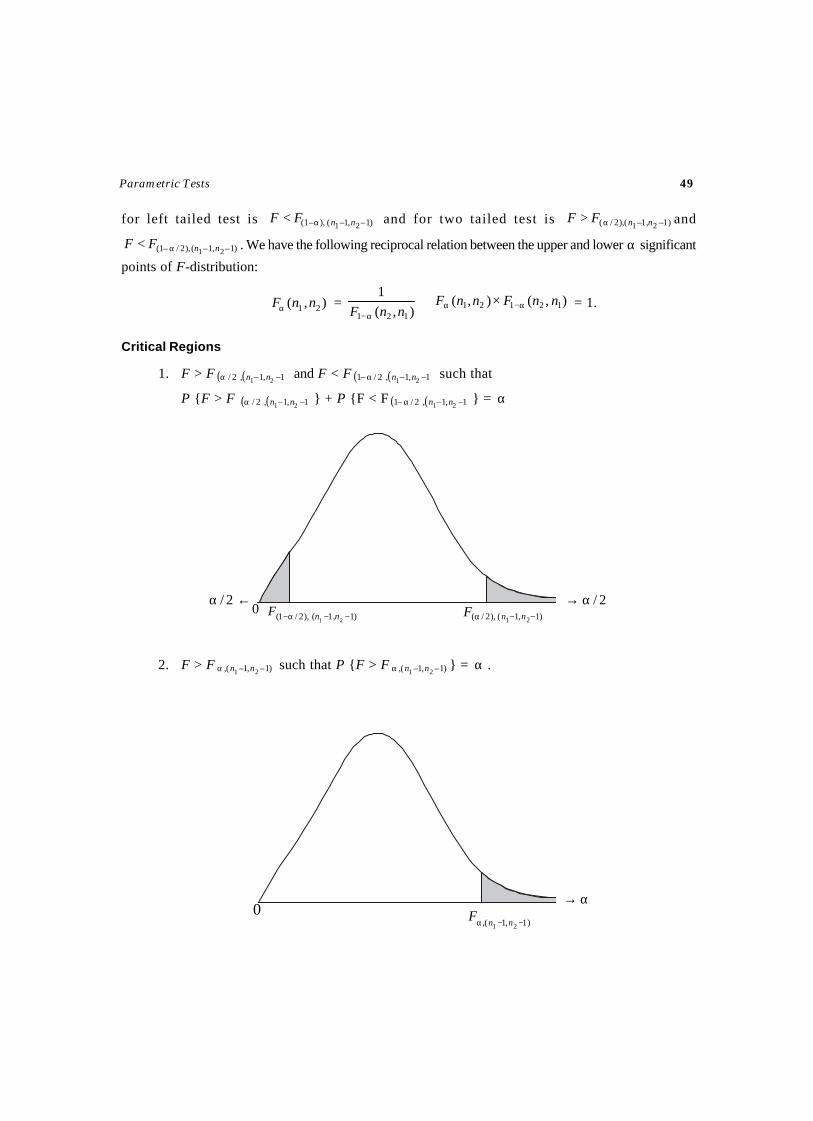
Parametric Tests 49
for left tailed test is )1–,1–(),–1( 21 nnFF α< and for two tailed test is )1–,1–(),2/( 21 nnFF α> and
)1–,1–(),2/–1( 21 nnFF α< . We have the following reciprocal relation between the upper and lower α significant
points of F-distribution:
),( 21 nnFα = ),(),(),(
112121
121
nnFnnFnnF α−α
α−
×⇒ = 1.
Critical Regions
1. F > F ( ) ( )1–,1–,2/ 21 nnα and F < F ( ) ( )1–,1–,2/–1 21 nnα such that
P {F > F ( ) ( )1–,1–,2/ 21 nnα } + P {F < F ( ) ( )1–,1–,2/–1 21 nnα } = α
2. F > F )1–,1–(, 21 nnα such that P {F > F )1–,1–(, 21 nnα } = α .
←α 2/ 2/α→0
)1,1(),2/1( 21 −−α− nnF )1,1(),2/( 21 −−α nnF
α→
)1,1(, 21 −−α nnF0
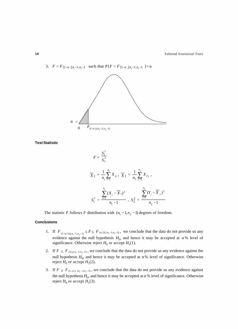
50 Selected Statistical Tests
3. F < F ( ) ( )111 21 –,–,– nnα such that P{F < F ( ) ( )111 21 –,–,– nnα }= α
Test Statistic
F = 22
21
S
S
1X = ∑=
1
11
1
1 n
iiX
n, 1X = ∑
=
2
12
2
1n
jjX
n,
21S =
1
)(
1
1
21
1
−
−∑=
n
XXn
ii
, 22S =
1
)(
2
1
22
2
−
−∑=
n
XYn
ji
The statistic F follows F distribution with )1,1( 21 −− nn degrees of freedom.
Conclusions
1. If F)1–,1–(),/2–1( 21 nnα ≤ F ≤ F )1–,1–(),/2( 21 nnα , we conclude that the data do not provide us any
evidence against the null hypothesis H0, and hence it may be accepted at α% level ofsignificance. Otherwise reject H0 or accept H1(1).
2. If F ≤ F )1–,1–(),( 21 nnα , we conclude that the data do not provide us any evidence against the
null hypothesis H0, and hence it may be accepted at α% level of significance. Otherwisereject H0 or accept H1(2).
3. If F ≥ F )1–,1–(),–1( 21 nnα , we conclude that the data do not provide us any evidence against
the null hypothesis H0, and hence it may be accepted at α% level of significance. Otherwisereject H0 or accept H1(3).
→α
0 )1–,1–(),–1( 21 nnF α
Parametric Tests 51
Example 1
A quality control supervisor for an automobile manufacturer is concerned with uniformity in thenumber of defects in cars coming off the assembly line. If one assembly line has significantly morevariability in the number of defects, then changes have to be made. The supervisor has obtained thefollowing data.
Number of Defects
Assembly Line-A Assembly Line-B
Mean 12 14
Variance 20 13
Sample size 16 20
Does assembly line A have significantly more variability in the number of defects? Test at 5%level of significance.
Solution
Aim: To test the assembly line A have significantly more variability than assembly line B in thenumber of defects or not.H0: There is no significant difference in variability between assembly line A and assembly line B inthe number of defects. i.e., H0: σ1
2 = σ22.
H1: The assembly line A has significantly more variability than assembly line B in the number ofdefects. i.e., H1: σ1
2 > σ22.
Level of Significance: α = 0.05 and Critical value: F0.05, (16-1, 20–1) = 2.23
Test Statistic: F = 22
21
S
S = 13
20 = 1.54
Conclusion: Since F < F),ná,(n 11 21 −−, we conclude that the data do not provide us any evidence
against the null hypothesis H0, and hence it is accepted at 5% level of significance. That is, there is nosignificant difference in variability between assembly line A and assembly line B in the number ofdefects.
Example 2
An insurance company is interested in the length of hospital-stays for various illnesses. Thecompany has selected 15 patients from hospital A and 10 from hospital B who were treated for thesame ailment. The amount of time spent in hospital A had an average of 2.6 days with a standarddeviation of 0.8 day. The treatment time in hospital B averaged 2.2 days with a standard deviation of0.12 day. Do patients in hospital A have significantly less variability in their recovery time? Test at 1%level of significance.
Solution
Aim: To test the patients in hospital A, have significantly less variability than the patients do inhospital B, in their recovery time.H0: There is no significant difference in recovery time in variability between the patients in hospitalA and hospital B. i.e., H0: σ1
2 = σ22.
52 Selected Statistical Tests
H1: The patients in hospital A, have significantly less variability than the patients do in hospital B,in their recovery time.i.e., H1: σ1
2 < σ22 ⇒ H1: σ2
2 > σ12.
Level of Significance: α = 0.01 and Critical value: F0.01, (10–1, 15–1) = 4.03.
Test Statistic: F = 21
22
S
S = 640
441..
= 2.25
Conclusion: Since F < F ( )1–,1–, 21 nnα, we conclude that the data do not provide us any evidence
against the null hypothesis H0 , and hence it is accepted at 5% level of significance. That is, patients athospital A do not have significantly less variability in their recovery times.
EXERCISES
1. Two brand managers were in disagreement over the issue of whether urban homemakers hadgreater variability in grocery shopping patterns than did rural homemakers. To test their conflictingideas, they took random samples of 25 homemakers from urban areas and 15 homemakers fromrural areas. They found that the variance for the urban homemaker was 4.25 and rural homemakerwas 3.5. Is the difference in the variances in days between shopping visits significant at 5% level?
2. The diameters of two random samples, each of size 10, of bullets produced by two machines havestandard deviations 0.012 and 0.018. Test the hypothesis that the two machines are equallyconsistent in diameters at 1% level of significance.

Aim
To test the given two attributes classified into two classes each, are independent, based on theobserved frequencies, obtained from any sample survey.
Source
A random sample of size N is classified into 2 classes by attribute-A and 2 classes by attribute-B.The above observed frequencies can be expressed in the following table known as 2 × 2 contingencytable as follows.
Attribute-A
Class–1 Class–2 Total
Class–1 a b a + b
Class–2 c d c + d
Total a + c b + d N
Assumptions
(i) The sample size N, should be sufficiently large (i.e., N > 20)(ii) Each cell frequencies should be independent.
(iii) Each cell frequencies are at least 3.
Null Hypothesis
H0: The two attributes are independent.
Alternative Hypothesis
H1: The two attributes are not independent.
TEST FOR CONSISTENCY IN A 2×2 TABLE
TEST – 14
Attribute–B
54 Selected Statistical Tests
Level of Significance ( αα) and Critical Region
χ2 > χ2α, (1) such that P{χ2 > χ2
α, (1)} = α
Test Statistic
χ2 =))()()((
}){( 2
dcdbcababcadN
++++−
The statistic χ2 follows χ2 distribution with one degree of freedom.
Conclusion
If χ2 ≤ χ2α,(1), we conclude that the data do not provide us any evidence against the null hypothesis
H0, and hence it may be accepted at α% level of significance. Otherwise reject H0 or accept H1.
Example 1
Out of 5000 households in a town, 3200 are self-employed, out of 2200 graduate households,1400 are self-employed. Examine whether there is any association between graduation and nature ofemployment at 5% level of significance.
Solution
Aim: To test the two attributes, graduation and nature of employment are independent.H0: Graduation and nature of employment are independent.H1: Graduation and nature of employment are dependent.Level of Significance: α = 0.05 and Critical value: χ2
0.05, 1 = 3.841
Employment
Self-empoyed Others
Graduates 1400 800 2200
Non-graduates 1800 1000 2800
Total 3200 1800 5000
Test Statistic: χ2 =))()()((
}){( 2
dcdbcababcadN
++++−
= 2800220018003200
)]8001800()10001400[(5000 2
××××−×
= 0.02
Conclusion: Since χ2 < χ2α, (1), we conclude that the data do not provide us any evidence against
the null hypothesis H0, and hence it is accepted at 5% level of significance. That is, Graduation andnature of employment are independent.
Example 2
A sample survey was conducted from 300 persons, to study the association between drinkinghabit and sales of liquor from a town. The following two questions were asked and their response isreported below.
Graduation Total
Parametric Tests 55
(A) Do you drink? (B) Are you in favor of sales of liquor?
Question-AYes No
Yes 100 40 140
No 140 20 160
Total 240 60 300
Test whether the drunkenness and opinion about the sales of liquor are associated or independentat 1% level of significance.
Solution
Aim: To test the drunkenness and opinion about the sales of liquor are associated or independent.H0: The drunkenness and opinion about the sales of liquor are independent.H1: The drunkenness and opinion about the sales of liquor are associated.Level of Significance: α = 0.05 and Critical value: χ2
0.05, 1 = 3.841
Test Statistic: χ2 =))()()((
}){( 2
dcdbcababcadN
++++−
=100240200140
)]14040()60100[(300 2
××××−×
= 0.071
Conclusion: Since χ2 < χ2α,(1), we conclude that the data do not provide us any evidence against
the null hypothesis H0, and hence it is accepted at 5% level of significance. That is, the drunkennessand opinion about the sales of liquor are independent.
EXERCISES
1. In an experiment on immunization of cattle from tuberculosis, the following data were obtained.
Affected Unaffected Total
Inoculated 12 68 80Not Inoculated 98 22 120
Total 110 90 200
Examine the effect of vaccine in controlling the incidence of the disease at 2% level.2. A sample survey was conducted from 500 to know the response from the students about the
introduction of CBCS system in the university. The following data were obtained:
Favor Against Total
Male 135 115 250Female 120 130 250
Total 255 245 500
Test whether the opinion about the introduction of CBCS system depends on the gender of thestudents at 2% level of significance.
Question-B Total
Aim
To test the k population proportions are equal based on k independent samples. That is to investigatethe significance of the difference among the k sample proportions.
Source
Let there be k populations from which k independent random samples are drawn. Let Oi be theobserved frequency of a specific kind obtained from the ith sample of ni observations, i = 1, 2,…, k.
Null Hypothesis
H0: The k population proportions are equal. That is, there is no significance difference among thek sample proportions.
i.e., H0: P1 = P2 = … = Pk.
Alternative Hypothesis
H1: P1 ≠ P2 ≠ … ≠ Pk.
Level of Significance ( αα) and Critical Region
χ2 < χ21-(α/2),(k-1) ∪ χ2 > χ2
(α/2),(k-1) such thatP{χ2 < χ2
1-(α/2),(k-1) ∪ χ2 > χ2(α/2),(k-1)} = α
Test Statistic
χ2 =( )∑
=
−k
i i
ii
pqnpnO
1
2
where p = ∑∑
i
i
n
O and q = 1–p.
The Statistic χ2 follows χ2 distribution with (k-1) degrees of freedom.
TEST FOR HOMOGENEITY OF SEVERAL
POPULATION PROPORTIONS
TEST – 15
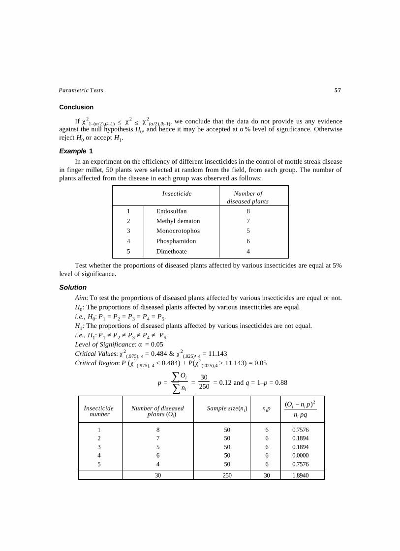
Parametric Tests 57
Conclusion
If χ21–(α/2),(k–1) ≤ χ2
≤ χ2(α/2),(k–1), we conclude that the data do not provide us any evidence
against the null hypothesis H0, and hence it may be accepted at α% level of significance. Otherwisereject H0 or accept H1.
Example 1
In an experiment on the efficiency of different insecticides in the control of mottle streak diseasein finger millet, 50 plants were selected at random from the field, from each group. The number ofplants affected from the disease in each group was observed as follows:
Insecticide Number ofdiseased plants
1 Endosulfan 8
2 Methyl dematon 7
3 Monocrotophos 5
4 Phosphamidon 6
5 Dimethoate 4
Test whether the proportions of diseased plants affected by various insecticides are equal at 5%level of significance.
Solution
Aim: To test the proportions of diseased plants affected by various insecticides are equal or not.H0: The proportions of diseased plants affected by various insecticides are equal.i.e., H0: P1 = P2 = P3 = P4 = P5.H1: The proportions of diseased plants affected by various insecticides are not equal.i.e., H1: P1 ≠ P2 ≠ P3 ≠ P4 ≠ P5.Level of Significance: α = 0.05Critical Values: χ2
(.975), 4 = 0.484 & χ2(.025), 4 = 11.143
Critical Region: P (χ2(.975), 4 < 0.484) + P(χ2
(.025),4 > 11.143) = 0.05
p = ∑∑
i
i
n
O = 250
30 = 0.12 and q = 1–p = 0.88
Insecticide Number of diseased Sample size(ni) nippqn
pnO
i
ii2)–(
1 8 50 6 0.75762 7 50 6 0.18943 5 50 6 0.18944 6 50 6 0.00005 4 50 6 0.7576
30 250 30 1.8940
number plants (Oi)
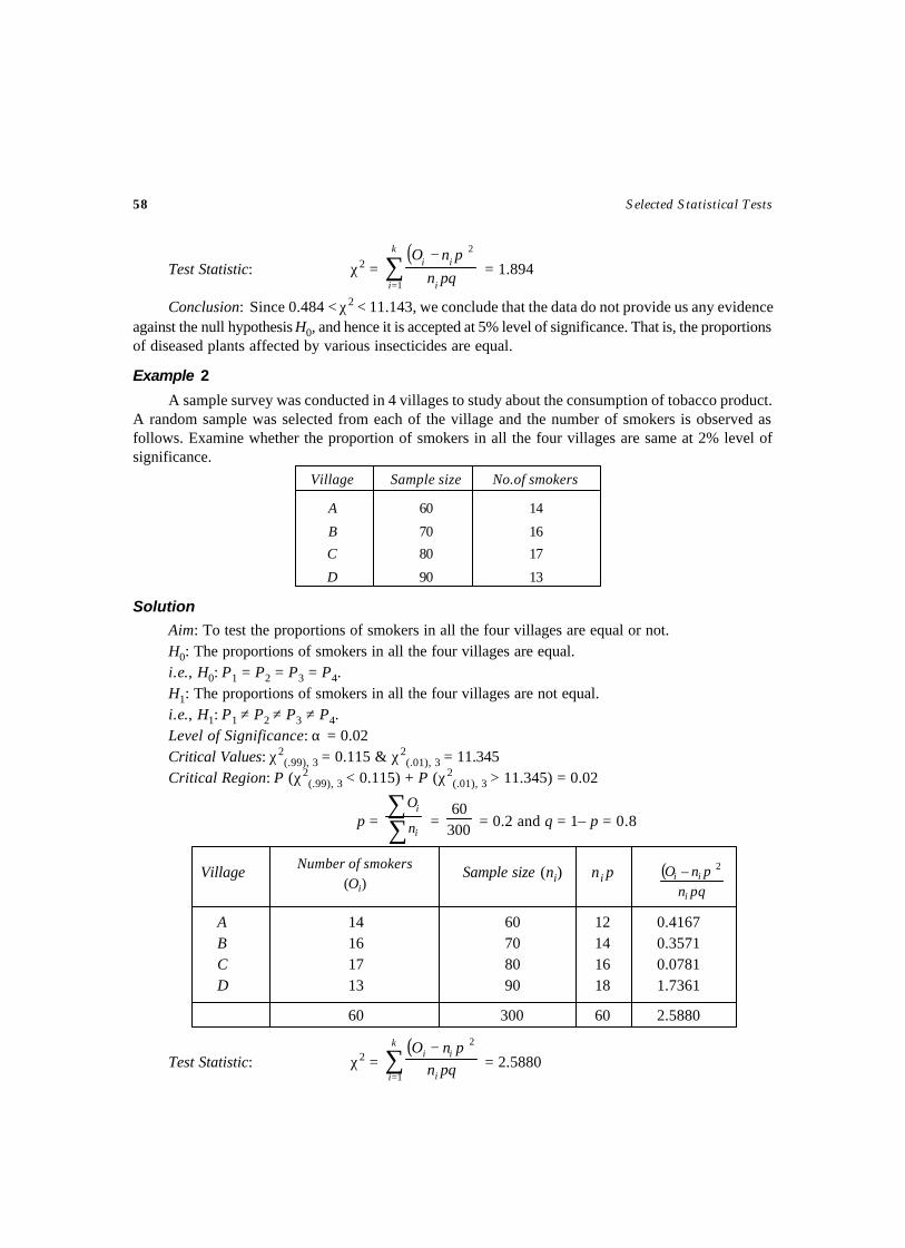
58 Selected Statistical Tests
Test Statistic: χ2 =( )∑
=
−k
i i
ii
pqn
pnO
1
2
= 1.894
Conclusion: Since 0.484 < χ2 < 11.143, we conclude that the data do not provide us any evidenceagainst the null hypothesis H0, and hence it is accepted at 5% level of significance. That is, the proportionsof diseased plants affected by various insecticides are equal.
Example 2
A sample survey was conducted in 4 villages to study about the consumption of tobacco product.A random sample was selected from each of the village and the number of smokers is observed asfollows. Examine whether the proportion of smokers in all the four villages are same at 2% level ofsignificance.
Village Sample size No.of smokers
A 60 14
B 70 16
C 80 17
D 90 13
Solution
Aim: To test the proportions of smokers in all the four villages are equal or not.H0: The proportions of smokers in all the four villages are equal.i.e., H0: P1 = P2 = P3 = P4.H1: The proportions of smokers in all the four villages are not equal.i.e., H1: P1 ≠ P2 ≠ P3 ≠ P4.Level of Significance: α = 0.02Critical Values: χ2
(.99), 3 = 0.115 & χ2(.01), 3 = 11.345
Critical Region: P (χ2(.99), 3 < 0.115) + P (χ2
(.01), 3 > 11.345) = 0.02
p = ∑∑
i
i
n
O = 300
60 = 0.2 and q = 1– p = 0.8
Village Sample size (ni) n i p ( )pqn
pnO
i
ii2–
A 14 60 12 0.4167B 16 70 14 0.3571C 17 80 16 0.0781D 13 90 18 1.7361
60 300 60 2.5880
Test Statistic: χ2 =( )∑
=
−k
i i
ii
pqnpnO
1
2
= 2.5880
Number of smokers(Oi)
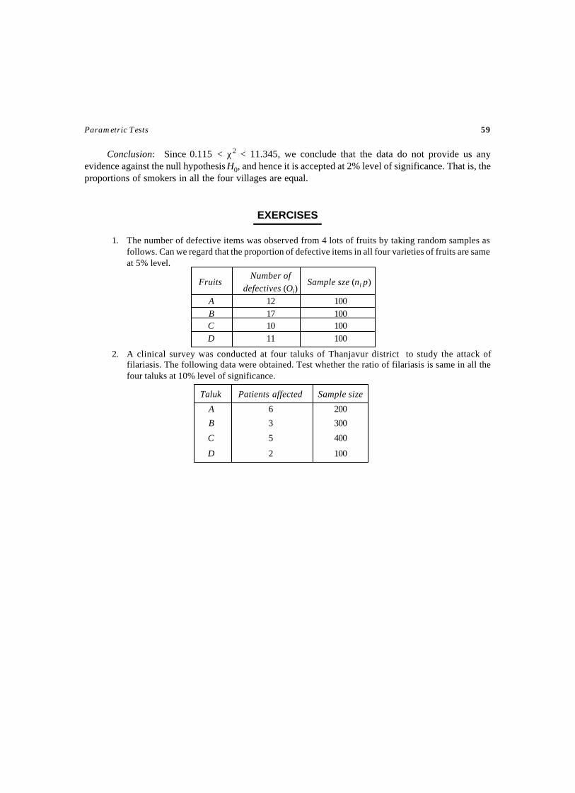
Parametric Tests 59
Conclusion: Since 0.115 < χ2 < 11.345, we conclude that the data do not provide us anyevidence against the null hypothesis H0, and hence it is accepted at 2% level of significance. That is, theproportions of smokers in all the four villages are equal.
EXERCISES
1. The number of defective items was observed from 4 lots of fruits by taking random samples asfollows. Can we regard that the proportion of defective items in all four varieties of fruits are sameat 5% level.
Number ofdefectives (Oi)
A 12 100B 17 100C 10 100D 11 100
2. A clinical survey was conducted at four taluks of Thanjavur district to study the attack offilariasis. The following data were obtained. Test whether the ratio of filariasis is same in all thefour taluks at 10% level of significance.
Taluk Patients affected Sample size
A 6 200
B 3 300
C 5 400
D 2 100
Fruits Sample sze (ni p)
Aim
To test the variances of the k populations are equal, based on k random samples. That is, toinvestigate the significance of the differences among k sample variances.
Source
Let Xij, ( i = 1, 2,…, k ; j = 1, 2,…, ni ) be the observations of k random samples each has ni
observations drawn from k independent populations whose variances are respectively 21σ , 2
2σ ,…, 2kσ .
Let 1X , 2X , …, kX be the means of k samples.
Assumptions
(i) The populations from which, the k samples drawn, are Normal distributions.
(ii) The unknown variances 21σ , 2
2σ ,…, 2kσ are estimated by their respective unbiased estimates
21S , 2
2S ,…, 2kS .
Null Hypothesis
H0: The variances of k populations 21σ , 2
2σ ,…, 2kσ are equal. That is, there is no significant
difference among the k unbiased estimates of the population variances 21S , 2
2S ,…, 2kS . i .e. ,
H0 : 21σ = 2
2σ = … = 2kσ .
Alternative Hypothesis
H1: 21σ ≠ 2
2σ ≠ … ≠ 2kσ .
Level of Significance ( αα) and Critical Region
χ2 < χ21–(α/2),(k–1) ∪ χ2 > χ2
(α/2),(k–1) such that
TEST FOR HOMOGENEITY OF SEVERAL
POPULATION VARIANCES
(BARTLETT'S TEST)
TEST – 16
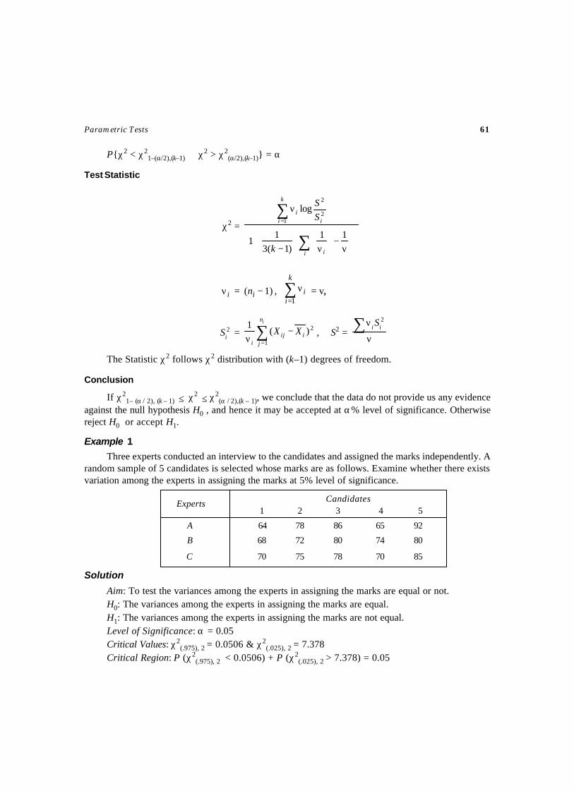
Parametric Tests 61
P{χ2 < χ21–(α/2),(k–1) ∪ χ2 > χ2
(α/2),(k–1)} = α
Test Statistic
χ2 =
ν−
ν−
+
ν
∑
∑=
11)1(3
11
log1
2
2
i i
k
i ii
k
SS
iν = )( 1−in , ∑=
νk
ii
1 = v,,
2iS = ∑
=
−ν
in
jiij
i
XX1
2)(1
, S2 = ν
ν∑ 2ii S
The Statistic χ2 follows χ2 distribution with (k–1) degrees of freedom.
Conclusion
If χ21– (α / 2), (k – 1) ≤ χ2 ≤ χ2
(α / 2),(k – 1), we conclude that the data do not provide us any evidenceagainst the null hypothesis H0 , and hence it may be accepted at α% level of significance. Otherwisereject H0 or accept H1.
Example 1
Three experts conducted an interview to the candidates and assigned the marks independently. Arandom sample of 5 candidates is selected whose marks are as follows. Examine whether there existsvariation among the experts in assigning the marks at 5% level of significance.
Candidates1 2 3 4 5
A 64 78 86 65 92
B 68 72 80 74 80
C 70 75 78 70 85
Solution
Aim: To test the variances among the experts in assigning the marks are equal or not.H0: The variances among the experts in assigning the marks are equal.H1: The variances among the experts in assigning the marks are not equal.Level of Significance: α = 0.05Critical Values: χ2
(.975), 2 = 0.0506 & χ2(.025), 2 = 7.378
Critical Region: P (χ2(.975), 2 < 0.0506) + P (χ2
(.025), 2 > 7.378) = 0.05
Experts
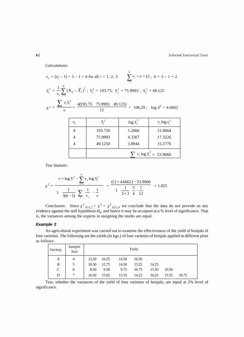
62 Selected Statistical Tests
Calculations:
iv = (ni – 1) = 5 – 1 = 4 for all i = 1, 2, 3 121
==∑=
vvk
ii ; k = 3 – 1 = 2
2iS = ∑
=
in
jiij
i
XXv 1
2)–(
1; 2
1S = 193.75; 22S = 75.9993 ; 2
3S = 49.125
2S = v
Sv ii∑ 2
= 12)125.499993.7575.193(4 ++
= 106.29 ; log S2 = 4.6662
iv 2iS 2log iS 2log ii sv
4 193.750 5.2666 21.0664
4 75.9993 4.3307 17.3226
4 49.1250 3.8944 15.5776
∑ 2log ii Sv = 53.9666
Test Statistic:
χ2 =
ν−
ν−
+
ν−×ν
∑
∑=
11)1(3
11
loglog1
22
i i
k
iii
k
SS
=
−
×+
−×
121
43
231
1
9666.53)6662.412( = 1.825
Conclusion: Since χ2.975,2 < χ2 < χ2
.025,2, we conclude that the data do not provide us anyevidence against the null hypothesis H0, and hence it may be accepted at α% level of significance. Thatis, the variances among the experts in assigning the marks are equal.
Example 2
An agricultural experiment was carried out to examine the effectiveness of the yield of brinjals offour varieties. The following are the yields (in kgs.) of four varieties of brinjals applied in different plotsas follows:
SampleSize
A 4 12.50 16.25 14.50 16.50B 5 10.50 12.75 14.50 13.25 14.25C 6 8.50 9.50 9.75 16.75 15.50 10.50
D 7 16.50 15.65 15.35 14.25 16.25 15.55 16.75
Test, whether the variances of the yield of four varieties of brinjals, are equal at 2% level ofsignificance.
YieldVariety
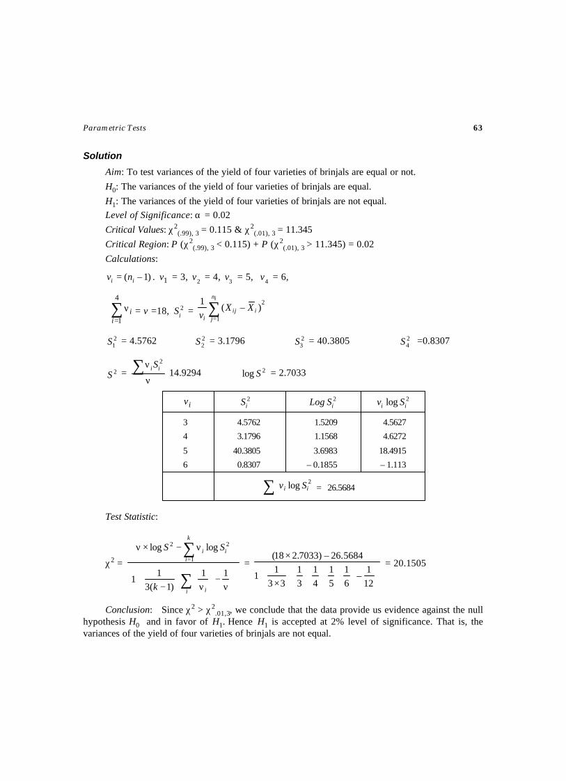
Parametric Tests 63
Solution
Aim: To test variances of the yield of four varieties of brinjals are equal or not.
H0: The variances of the yield of four varieties of brinjals are equal.
H1: The variances of the yield of four varieties of brinjals are not equal.Level of Significance: α = 0.02
Critical Values: χ2(.99), 3 = 0.115 & χ2
(.01), 3 = 11.345
Critical Region: P (χ2(.99), 3 < 0.115) + P (χ2
(.01), 3 > 11.345) = 0.02
Calculations:
)1–( ii nv = . 1v = 3, 2v = 4, 3v = 5, 4v = 6,
∑=
ν4
1ii = v =18, 2
iS = ∑=
in
jiij
i
XXv 1
2)–(
1
21S = 4.5762 2
2S = 3.1796 23S = 40.3805 2
4S =0.8307
2S = ν
ν∑ 2ii S 14.9294 2log S = 2.7033
iv 2iS 2
iSLog 2log ii Sv
3 4.5762 1.5209 4.5627
4 3.1796 1.1568 4.6272
5 40.3805 3.6983 18.4915
6 0.8307 – 0.1855 – 1.113
∑ 2log ii Sv = 26.5684
Test Statistic:
χ2 =
ν−
ν−
+
ν−×ν
∑
∑=
11)1(3
11
loglog1
22
i i
k
iii
k
SS
=
+++
×+
×
121
–61
51
41
31
331
1
5684.26–)7033.218( = 20.1505
Conclusion: Since χ2 > χ2.01,3, we conclude that the data provide us evidence against the null
hypothesis H0 and in favor of H1. Hence H1 is accepted at 2% level of significance. That is, thevariances of the yield of four varieties of brinjals are not equal.
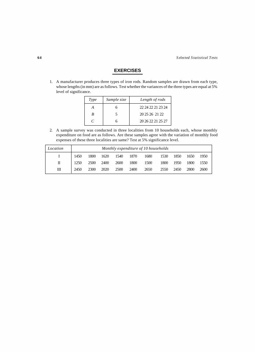
64 Selected Statistical Tests
EXERCISES
1. A manufacturer produces three types of iron rods. Random samples are drawn from each type,whose lengths (in mm) are as follows. Test whether the variances of the three types are equal at 5%level of significance.
Type Sample size Length of rods
A 6 22 24 22 21 23 24
B 5 20 25 26 21 22
C 6 20 26 22 21 25 27
2. A sample survey was conducted in three localities from 10 households each, whose monthlyexpenditure on food are as follows. Are these samples agree with the variation of monthly foodexpenses of these three localities are same? Test at 5% significance level.
Location Monthly expenditure of 10 households
I 1450 1800 1620 1540 1870 1680 1530 1850 1650 1950
II 1250 2500 2400 2600 1800 1500 1800 1950 1800 1550
III 2450 2300 2020 2500 2400 2650 2550 2450 2800 2600
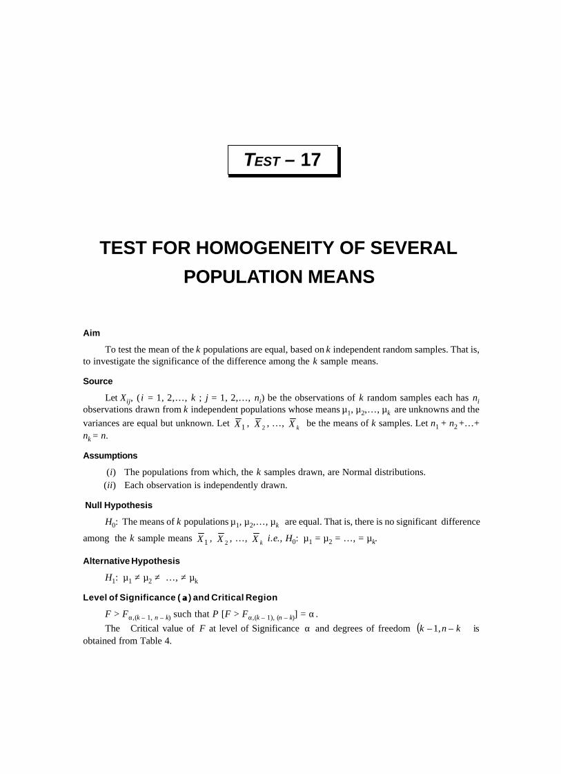
Aim
To test the mean of the k populations are equal, based on k independent random samples. That is,to investigate the significance of the difference among the k sample means.
Source
Let Xij, ( i = 1, 2,…, k ; j = 1, 2,…, ni) be the observations of k random samples each has niobservations drawn from k independent populations whose means µ1, µ2,…, µk are unknowns and thevariances are equal but unknown. Let 1X , 2X , …, kX be the means of k samples. Let n1 + n2 +…+nk = n.
Assumptions
(i) The populations from which, the k samples drawn, are Normal distributions.(ii) Each observation is independently drawn.
Null Hypothesis
H0: The means of k populations µ1, µ2,…, µk are equal. That is, there is no significant difference
among the k sample means 1X , 2X , …, kX i.e., H0: µ1 = µ2 = …, = µk.
Alternative Hypothesis
H1: µ1 ≠ µ2 ≠ …, ≠ µk
Level of Significance ( αα) and Critical Region
F > Fα,(k – 1, n – k) such that P [F > Fα,(k – 1), (n – k)] = α .
The Critical value of F at level of Significance α and degrees of freedom ( )knk –,– 1 isobtained from Table 4.
TEST FOR HOMOGENEITY OF SEVERAL
POPULATION MEANS
TEST – 17
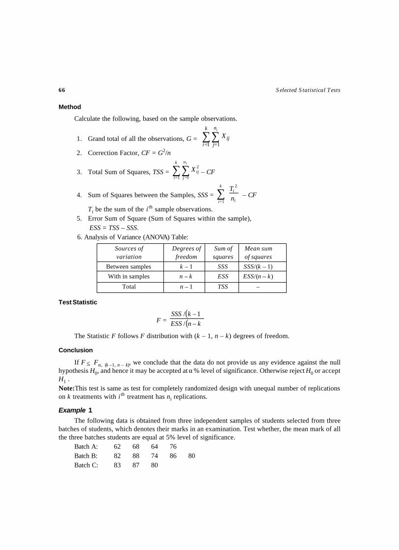
66 Selected Statistical Tests
Method
Calculate the following, based on the sample observations.
1. Grand total of all the observations, G = ∑∑= =
k
i
n
jij
i
X1 1
2. Correction Factor, CF = G2/n
3. Total Sum of Squares, TSS = ∑∑= =
k
i
n
jij
i
X1 1
2– CF
4. Sum of Squares between the Samples, SSS = ∑=
k
i i
i
nT
1
2
– CF
Ti be the sum of the i th sample observations.5. Error Sum of Square (Sum of Squares within the sample),
ESS = TSS – SSS.6. Analysis of Variance (ANOVA) Table:
Sources of Degrees of Sum of Mean sumvariation freedom squares of squares
Between samples k – 1 SSS SSS/(k – 1)
With in samples n – k ESS ESS/(n – k)
Total n – 1 TSS –
Test Statistic
F =( )( )knESSkSSS
–/–/ 1
The Statistic F follows F distribution with (k – 1, n – k) degrees of freedom.
Conclusion
If F ≤ Fα, (k –1, n – k), we conclude that the data do not provide us any evidence against the nullhypothesis H0, and hence it may be accepted at α% level of significance. Otherwise reject H0 or acceptH1 .Note:This test is same as test for completely randomized design with unequal number of replicationson k treatments with i th treatment has ni replications.
Example 1
The following data is obtained from three independent samples of students selected from threebatches of students, which denotes their marks in an examination. Test whether, the mean mark of allthe three batches students are equal at 5% level of significance.
Batch A: 62 68 64 76Batch B: 82 88 74 86 80Batch C: 83 87 80
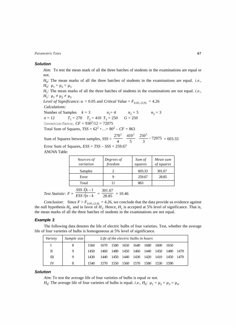
Parametric Tests 67
Solution
Aim: To test the mean mark of all the three batches of students in the examinations are equal ornot.H0: The mean marks of all the three batches of students in the examinations are equal. i.e.,H0: µ1 = µ2 = µ3
H1: The mean marks of all the three batches of students in the examinations are not equal. i.e.,H1: µ1 ≠ µ2 ≠ µ3
Level of Significance: α = 0.05 and Critical Value = F0.05, (2,9) = 4.26Calculations:Number of Samples k = 3 n1= 4 n2 = 5 n3 = 3n = 12 T1 = 270 T2 = 410 T3 = 250 G = 250Correction Factor, CF = 9302/12 = 72075Total Sum of Squares, TSS = 622 +…+ 802 – CF = 863
Sum of Squares between samples, SSS = 720753
2505
4104
270 222
−++ = 603.33
Error Sum of Squares, ESS = TSS – SSS = 259.67ANOVA Table:
Sources of Degrees of Sum of Mean sumvariation freedom squares of squares
Samples 2 603.33 301.67
Error 9 259.67 28.85
Total 11 863
Test Statistic: F = ( )( )knESSkSSS
–/–/ 1
= 85.2867.301
= 10.46
Conclusion: Since F > F0.05, (2,9) = 4.26, we conclude that the data provide us evidence againstthe null hypothesis H0 and in favor of H1. Hence, H1 is accepted at 5% level of significance. That is,the mean marks of all the three batches of students in the examinations are not equal.
Example 2
The following data denotes the life of electric bulbs of four varieties. Test, whether the averagelife of four varieties of bulbs is homogeneous at 5% level of significance.
Variety Sample size Life of the electric bulbs in hours
I 8 1560 1670 1580 1650 1640 1680 1600 1650
II 9 1450 1460 1480 1450 1460 1440 1450 1480 1470
III 9 1430 1440 1450 1440 1430 1420 1410 1450 1470
IV 8 1540 1570 1550 1560 1570 1580 1530 1590
Solution
Aim: To test the average life of four varieties of bulbs is equal or not.H0: The average life of four varieties of bulbs is equal. i.e., H0: µ1 = µ2 = µ3 = µ4.
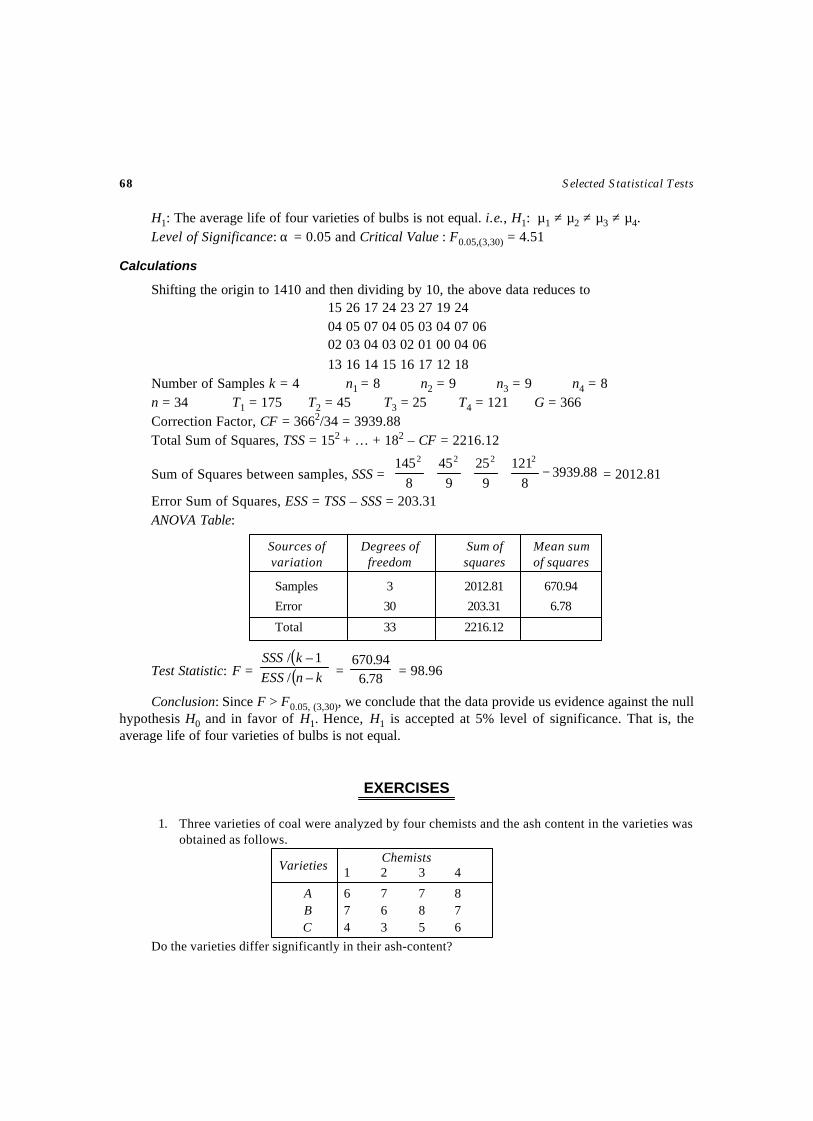
68 Selected Statistical Tests
H1: The average life of four varieties of bulbs is not equal. i.e., H1: µ1 ≠ µ2 ≠ µ3 ≠ µ4.Level of Significance: α = 0.05 and Critical Value : F0.05,(3,30) = 4.51
Calculations
Shifting the origin to 1410 and then dividing by 10, the above data reduces to15 26 17 24 23 27 19 2404 05 07 04 05 03 04 07 0602 03 04 03 02 01 00 04 0613 16 14 15 16 17 12 18
Number of Samples k = 4 n1 = 8 n2 = 9 n3 = 9 n4 = 8n = 34 T1 = 175 T2 = 45 T3 = 25 T4 = 121 G = 366Correction Factor, CF = 3662/34 = 3939.88Total Sum of Squares, TSS = 152 + … + 182 – CF = 2216.12
Sum of Squares between samples, SSS = 88.39398
1219
259
458
145 2222
−+++ = 2012.81
Error Sum of Squares, ESS = TSS – SSS = 203.31ANOVA Table:
Sources of Degrees of Sum of Mean sumvariation freedom squares of squares
Samples 3 2012.81 670.94
Error 30 203.31 6.78
Total 33 2216.12
Test Statistic: F = ( )( )knESSkSSS
–/–/ 1
= 78.694.670
= 98.96
Conclusion: Since F > F0.05, (3,30), we conclude that the data provide us evidence against the nullhypothesis H0 and in favor of H1. Hence, H1 is accepted at 5% level of significance. That is, theaverage life of four varieties of bulbs is not equal.
EXERCISES
1. Three varieties of coal were analyzed by four chemists and the ash content in the varieties wasobtained as follows.
Chemists1 2 3 4
A 6 7 7 8B 7 6 8 7C 4 3 5 6
Do the varieties differ significantly in their ash-content?
Varieties

Parametric Tests 69
2. Three processes A, B and C are tested to see whether their outputs are equivalent. The followingobservations of output are made:
A 12 15 17 18 15 17 16
B 14 17 18 14 16 14
C 14 18 17 15 15 19 17 19
Examine the outputs of these three processes differ significantly at 1% level of significance.

Aim
To test the given two attributes are independent, based on the observed frequencies, obtainedfrom any sample survey.
Source
A random sample of N observed frequencies be classified into m classes by attribute-A and nclasses by attribute-B. The above observed frequencies can be expressed in the following table knownas m × n contingency table.
Attribute-B1 2 … j … n
1 O11 O12 … O1j … O1n O1.
2 O21 O22 … O2j … O2n O2.
… … … … … … … …
… … … … … … … …
… … … … … … … …
Attribute i Oi1 Oi2 … Oij … Oin Oi.
A … … … … … … … …
… … … … … … … …
… … … … … … … …
m Om1 Om2 … Omj … Omn Om.
Total O.1 O.2 … O.j … O.n N
Assumptions
(i) The sample size N, should be sufficiently large.(ii) Each cell frequencies Oij should be independent.
(iii) Each cell frequencies Oij should be at least 5.
TEST FOR INDEPENDENCE OF
ATTRIBUTES
TEST – 18
Total
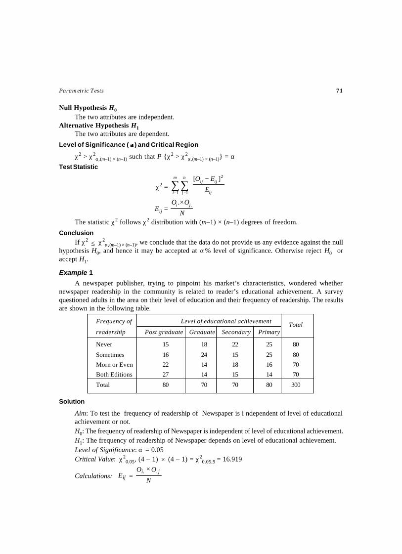
Parametric Tests 71
Null Hypothesis H0The two attributes are independent.
Alternative Hypothesis H1The two attributes are dependent.
Level of Significance ( αα) and Critical Region
χ2 > χ2α,(m–1) × (n–1) such that P {χ2 > χ2
α,(m–1) × (n–1)} = αTest Statistic
χ2 = ∑∑= =
−m
i
n
j ij
ijij
E
EO
1 1
2][
Eij =N
OO ji ..×
The statistic χ2 follows χ2 distribution with (m–1) × (n–1) degrees of freedom.
ConclusionIf χ2 ≤ χ2
α,(m–1) × (n–1), we conclude that the data do not provide us any evidence against the nullhypothesis H0, and hence it may be accepted at α% level of significance. Otherwise reject H0 oraccept H1.
Example 1
A newspaper publisher, trying to pinpoint his market’s characteristics, wondered whethernewspaper readership in the community is related to reader’s educational achievement. A surveyquestioned adults in the area on their level of education and their frequency of readership. The resultsare shown in the following table.
Frequency of Level of educational achievement
readership Post graduate Graduate Secondary Primary
Never 15 18 22 25 80
Sometimes 16 24 15 25 80
Morn or Even 22 14 18 16 70
Both Editions 27 14 15 14 70
Total 80 70 70 80 300
Solution
Aim: To test the frequency of readership of Newspaper is i ndependent of level of educationalachievement or not.H0: The frequency of readership of Newspaper is independent of level of educational achievement.H1: The frequency of readership of Newspaper depends on level of educational achievement.Level of Significance: α = 0.05Critical Value: χ2
0.05, (4 – 1) × (4 – 1) = χ20.05,9 = 16.919
Calculations: ijE = N
OO ji .. ×
Total
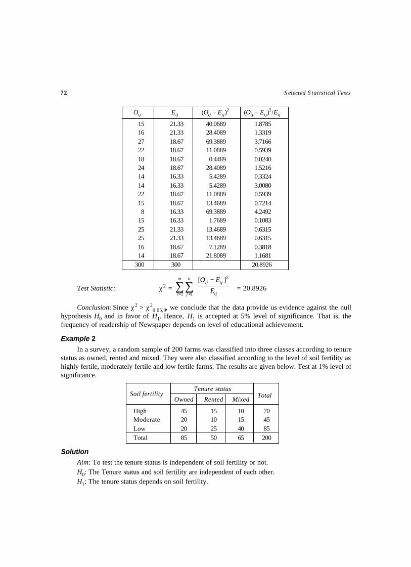
72 Selected Statistical Tests
Oij Eij (Oij – Eij)2 (Oij – Eij)
2/Eij
15 21.33 40.0689 1.878516 21.33 28.4089 1.331927 18.67 69.3889 3.716622 18.67 11.0889 0.593918 18.67 0.4489 0.024024 18.67 28.4089 1.521614 16.33 5.4289 0.332414 16.33 5.4289 3.008022 18.67 11.0889 0.593915 18.67 13.4689 0.72148 16.33 69.3889 4.2492
15 16.33 1.7689 0.108325 21.33 13.4689 0.631525 21.33 13.4689 0.631516 18.67 7.1289 0.381814 18.67 21.8089 1.1681
300 300 20.8926
Test Statistic: χ2 = ∑∑= =
−m
i
n
j ij
ijij
E
EO
1 1
2][ = 20.8926
Conclusion: Since χ2 > χ20.05,9, we conclude that the data provide us evidence against the null
hypothesis H0 and in favor of H1. Hence, H1 is accepted at 5% level of significance. That is, thefrequency of readership of Newspaper depends on level of educational achievement.
Example 2
In a survey, a random sample of 200 farms was classified into three classes according to tenurestatus as owned, rented and mixed. They were also classified according to the level of soil fertility ashighly fertile, moderately fertile and low fertile farms. The results are given below. Test at 1% level ofsignificance.
Tenure status
Owned Rented Mixed
High 45 15 10 70Moderate 20 10 15 45Low 20 25 40 85Total 85 50 65 200
Solution
Aim: To test the tenure status is independent of soil fertility or not.H0: The Tenure status and soil fertility are independent of each other.H1: The tenure status depends on soil fertility.
Soil fertility Total
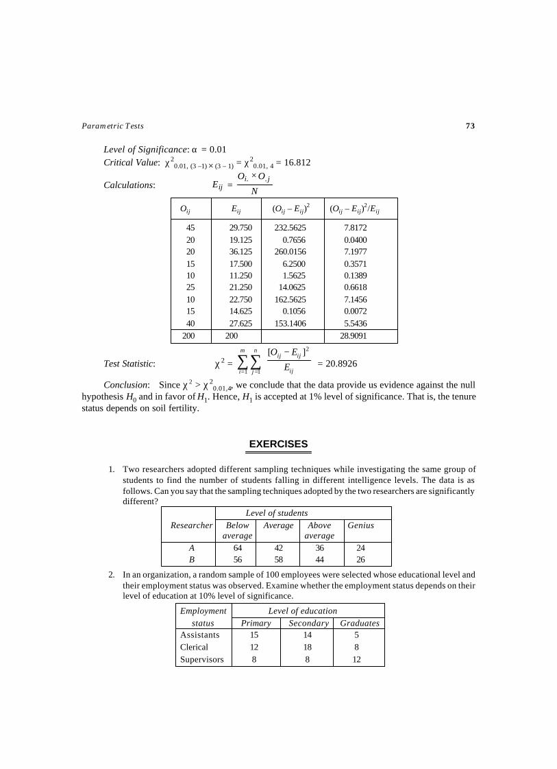
Parametric Tests 73
Level of Significance: α = 0.01Critical Value: χ2
0.01, (3 –1) × (3 – 1) = χ20.01, 4 = 16.812
Calculations: ijE =N
OO ji .. ×
Oij Eij (Oij – Eij)2 (Oij – Eij)
2/Eij
45 29.750 232.5625 7.817220 19.125 0.7656 0.040020 36.125 260.0156 7.197715 17.500 6.2500 0.357110 11.250 1.5625 0.138925 21.250 14.0625 0.661810 22.750 162.5625 7.145615 14.625 0.1056 0.007240 27.625 153.1406 5.5436
200 200 28.9091
Test Statistic: χ2 = ∑∑= =
−m
i
n
j ij
ijij
E
EO
1 1
2][= 20.8926
Conclusion: Since χ2 > χ20.01,4, we conclude that the data provide us evidence against the null
hypothesis H0 and in favor of H1. Hence, H1 is accepted at 1% level of significance. That is, the tenurestatus depends on soil fertility.
EXERCISES
1. Two researchers adopted different sampling techniques while investigating the same group ofstudents to find the number of students falling in different intelligence levels. The data is asfollows. Can you say that the sampling techniques adopted by the two researchers are significantlydifferent?
Level of studentsResearcher Below Average Above Genius
average averageA 64 42 36 24B 56 58 44 26
2. In an organization, a random sample of 100 employees were selected whose educational level andtheir employment status was observed. Examine whether the employment status depends on theirlevel of education at 10% level of significance.
Employment Level of educationstatus Primary Secondary Graduates
Assistants 15 14 5Clerical 12 18 8Supervisors 8 8 12
TEST FOR POPULATION CORRELATION
COEFFICIENT EQUALS ZERO
TEST – 19
Aim
To test the population correlation coefficient is zero, based on a bivariate random sample. That is,to investigate the significance of the difference between the sample correlation coefficient r and zero.
Source
Let (Xi, Yi), ( i = 1, 2,…, n) be a random sample of n pairs of observations drawn from a bivariatenormal population whose correlation coefficient ρ is unknown. Let r be the correlation coefficientbased on the above sample.
Assumptions
(i) The population from which, the sample drawn, is a bivariate normal population.(ii) The relationship between X and Y is linear.
Null Hypothesis
H0: The population correlation coefficient ρ is zero. That is, there is no significant differencebetween the sample correlation coefficient r and zero. i.e., H0: ρ = 0
Alternative Hypothesis
H1: ρ ≠ 0
Level of Significance ( αα) and Critical Region
| t | > tα,(n–2) such that P{| t | > tα,(n–2)} = α
Test Statistic
t = 2––1 2
nr
r

Parametric Tests 75
r =2222 11
1
∑∑
∑
−
−
−
YYn
XXn
YXXYn
The statistic t follows t distribution with (n–2) degrees of freedom.
Conclusion
If | t | ≤ tα, we conclude that the data do not provide us any evidence against the null hypothesisH0, be accepted at α% level of significance. Otherwise reject H0 or accept H1.
Example 1
A random sample of 10 student’s marks in Mathematics and English are given below. Test whetherthe correlation exists between the marks of two subjects at 2% level of significance.
Marks in Mathematics: 68 54 78 75 76 85 54 68 87 75Marks in English: 59 68 72 67 72 78 64 58 68 74
Solution
Aim: To test the correlation coefficient between the marks in mathematics and English is zero ornot.H0: The correlation coefficient between the marks in Mathematics and English is zero i.e. ,H0 : ρ = 0H1: The correlation coefficient between the marks in Mathematics and English is not zero i.e.,H1 : ρ ≠ 0Level of Significance: α = 0.02 and Critical Value: t0.02,8 = 2.896Based on the data,
∑ X = 720 ; ∑ Y = 680 ; 2∑ X = 52984 ;
2∑Y = 46606 ; ∑ XY = 49293
r =2222 11
1
∑∑
∑
−
−
−
YYn
XXn
YXXYn
=
−×
−×
×−
×
22 6846606101
7252984101
)6872(49293101
= 0.51
Test Statistic: t = 21 2
−−
nr
r = 0.51 × 2.83/0.86 = 1.68
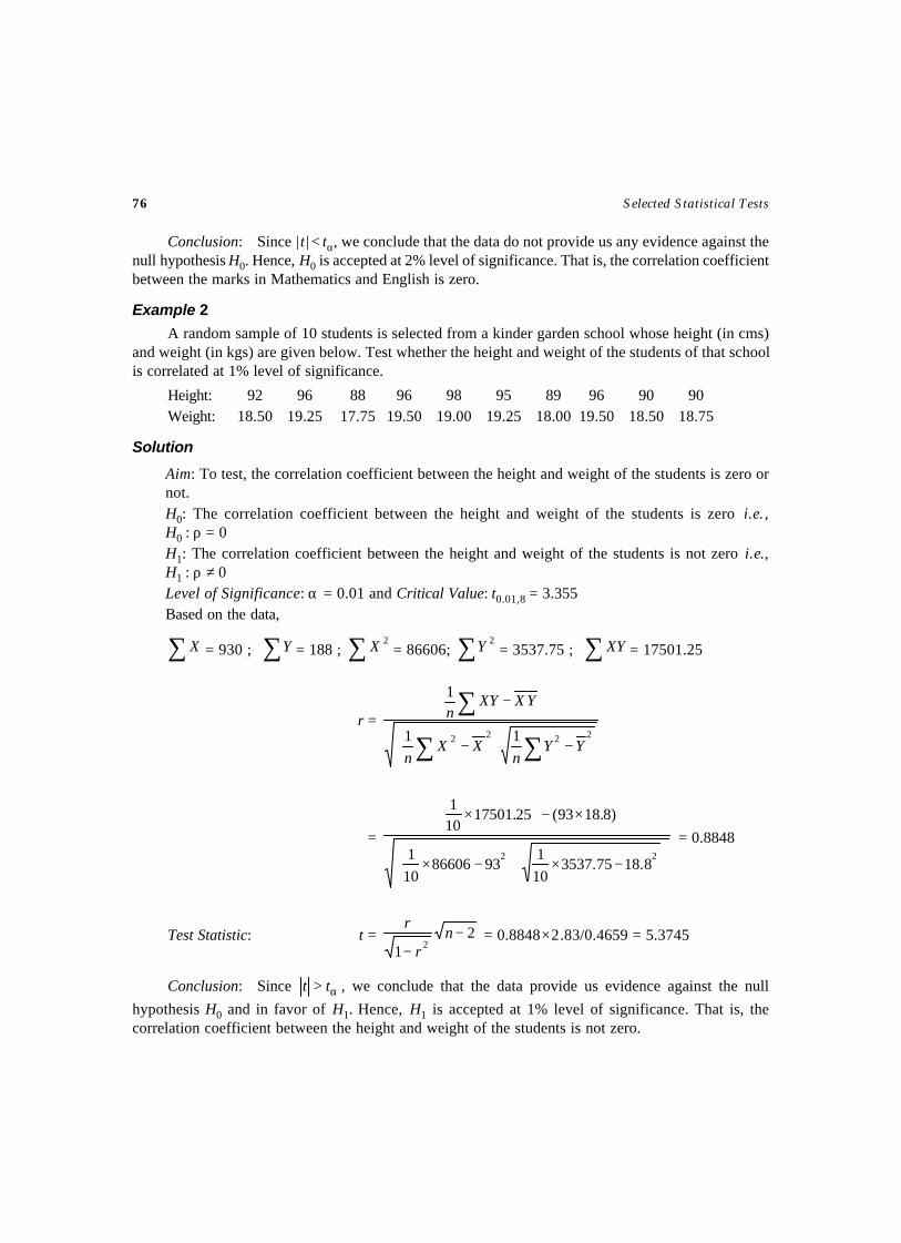
76 Selected Statistical Tests
Conclusion: Since | t | < tα, we conclude that the data do not provide us any evidence against thenull hypothesis H0. Hence, H0 is accepted at 2% level of significance. That is, the correlation coefficientbetween the marks in Mathematics and English is zero.
Example 2
A random sample of 10 students is selected from a kinder garden school whose height (in cms)and weight (in kgs) are given below. Test whether the height and weight of the students of that schoolis correlated at 1% level of significance.
Height: 92 96 88 96 98 95 89 96 90 90Weight: 18.50 19.25 17.75 19.50 19.00 19.25 18.00 19.50 18.50 18.75
Solution
Aim: To test, the correlation coefficient between the height and weight of the students is zero ornot.H0: The correlation coefficient between the height and weight of the students is zero i.e. ,H0 : ρ = 0H1: The correlation coefficient between the height and weight of the students is not zero i.e.,H1 : ρ ≠ 0Level of Significance: α = 0.01 and Critical Value: t0.01,8 = 3.355Based on the data,
∑ X = 930 ; ∑Y = 188 ; ∑ 2X = 86606; ∑ 2Y = 3537.75 ; ∑ XY = 17501.25
r =2222 11
1
∑∑
∑
−
−
−
YYn
XXn
YXXYn
=
−×
−×
×−
×
228.1875.3537
101
9386606101
)8.1893(25.17501101
= 0.8848
Test Statistic: t = 21 2
−−
nr
r = 0.8848×2.83/0.4659 = 5.3745
Conclusion: Since α> tt , we conclude that the data provide us evidence against the null
hypothesis H0 and in favor of H1. Hence, H1 is accepted at 1% level of significance. That is, thecorrelation coefficient between the height and weight of the students is not zero.
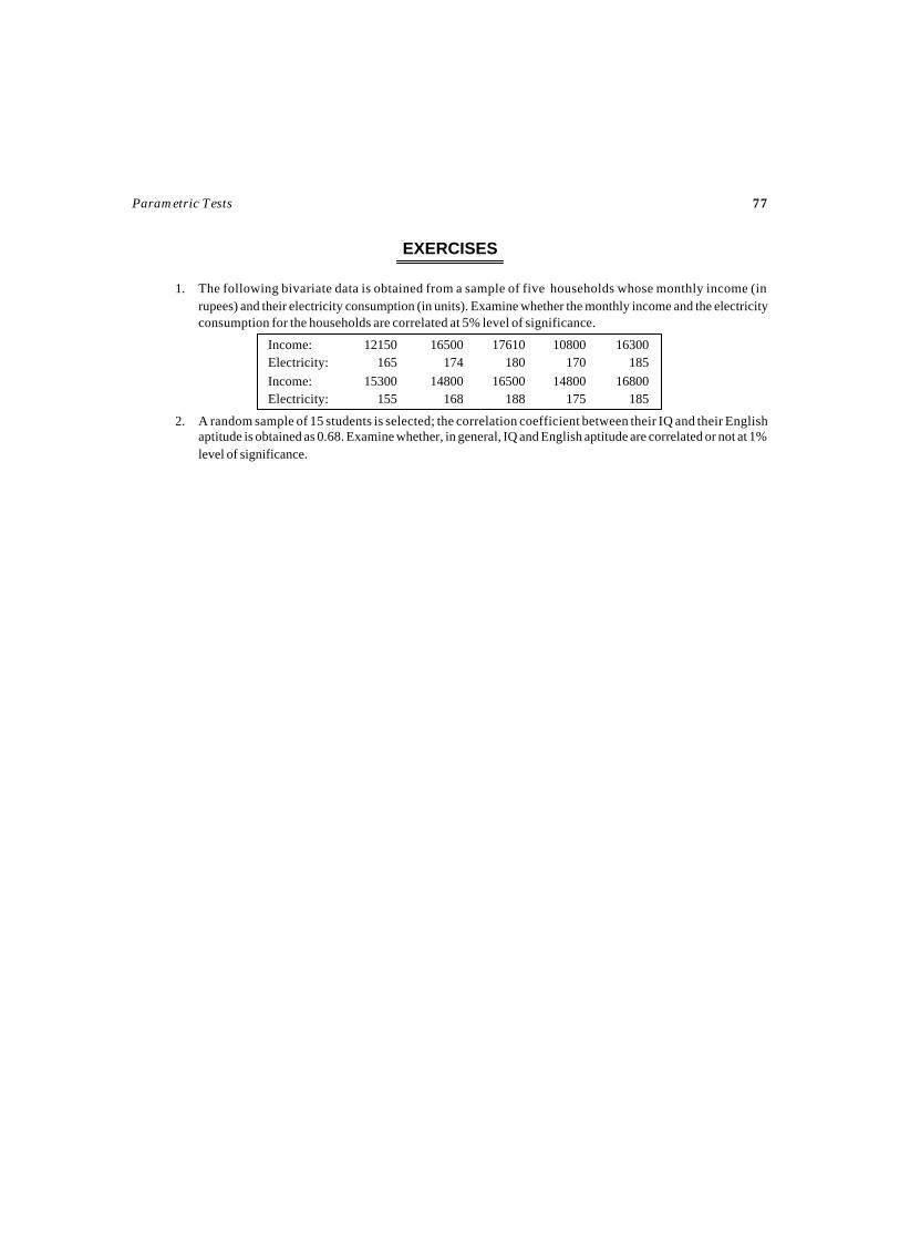
Parametric Tests 77
EXERCISES
1. The following bivariate data is obtained from a sample of five households whose monthly income (inrupees) and their electricity consumption (in units). Examine whether the monthly income and the electricityconsumption for the households are correlated at 5% level of significance.
Income: 12150 16500 17610 10800 16300Electricity: 165 174 180 170 185Income: 15300 14800 16500 14800 16800Electricity: 155 168 188 175 185
2. A random sample of 15 students is selected; the correlation coefficient between their IQ and their Englishaptitude is obtained as 0.68. Examine whether, in general, IQ and English aptitude are correlated or not at 1%level of significance.
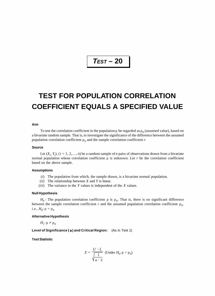
TEST FOR POPULATION CORRELATION
COEFFICIENT EQUALS A SPECIFIED VALUE
TEST – 20
Aim
To test the correlation coefficient in the population ρ be regarded as ρ0 (assumed value), based ona bivariate random sample. That is, to investigate the significance of the difference between the assumedpopulation correlation coefficient ρ0 and the sample correlation coefficient r.
Source
Let (Xi, Yi), ( i = 1, 2,…, n) be a random sample of n pairs of observations drawn from a bivariatenormal population whose correlation coefficient ρ is unknown. Let r be the correlation coefficientbased on the above sample.
Assumptions
(i) The population from which, the sample drawn, is a bivariate normal population.(ii) The relationship between X and Y is linear.
(iii) The variance in the Y values is independent of the X values.
Null Hypothesis
H0 : The population correlation coefficient ρ is ρ0. That is, there is no significant differencebetween the sample correlation coefficient r and the assumed population correlation coefficient ρ0.i.e., H0: ρ = ρ0
Alternative Hypothesis
H1: ρ ≠ ρ0
Level of Significance ( αα) and Critical Region: (As in Test 1)
Test Statistic
Z =
31−
ξ−
n
U (Under H0: ρ = ρ0)
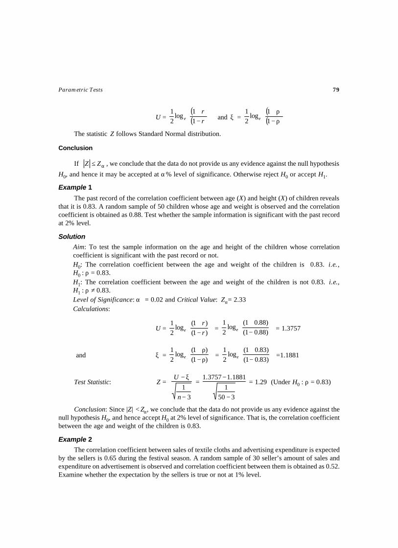
Parametric Tests 79
U =( )( )
−+
rr
e 11
log21
and ξ = ( )( )
ρ−ρ+
11
log21
e
The statistic Z follows Standard Normal distribution.
Conclusion
If α≤ ZZ , we conclude that the data do not provide us any evidence against the null hypothesis
H0, and hence it may be accepted at α% level of significance. Otherwise reject H0 or accept H1.
Example 1
The past record of the correlation coefficient between age (X) and height (X) of children revealsthat it is 0.83. A random sample of 50 children whose age and weight is observed and the correlationcoefficient is obtained as 0.88. Test whether the sample information is significant with the past recordat 2% level.
Solution
Aim: To test the sample information on the age and height of the children whose correlationcoefficient is significant with the past record or not.H0: The correlation coefficient between the age and weight of the children is 0.83. i.e. ,H0 : ρ = 0.83.H1: The correlation coefficient between the age and weight of the children is not 0.83. i.e.,H1 : ρ ≠ 0.83.Level of Significance: α = 0.02 and Critical Value: Zα= 2.33Calculations:
U =
−+
)1()1(
log21
rr
e =
−+
)88.01()88.01(
log21
e = 1.3757
and ξ =
ρ−ρ+)1()1(
log21
e =
−+
)83.01()83.01(
log21
e =1.1881
Test Statistic: Z =
31−
ξ−
n
U =
3501
1881.13757.1
−
− = 1.29 (Under H0 : ρ = 0.83)
Conclusion: Since |Z| < Zα, we conclude that the data do not provide us any evidence against thenull hypothesis H0, and hence accept H0 at 2% level of significance. That is, the correlation coefficientbetween the age and weight of the children is 0.83.
Example 2
The correlation coefficient between sales of textile cloths and advertising expenditure is expectedby the sellers is 0.65 during the festival season. A random sample of 30 seller’s amount of sales andexpenditure on advertisement is observed and correlation coefficient between them is obtained as 0.52.Examine whether the expectation by the sellers is true or not at 1% level.
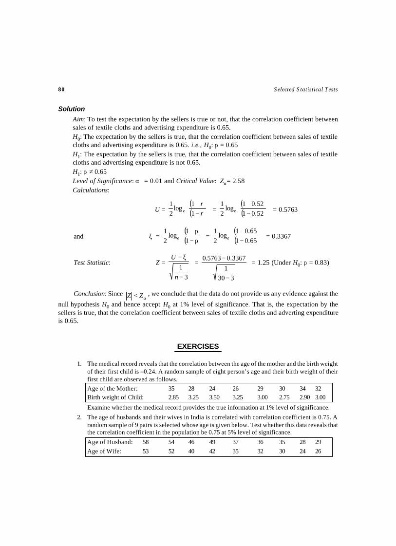
80 Selected Statistical Tests
Solution
Aim: To test the expectation by the sellers is true or not, that the correlation coefficient betweensales of textile cloths and advertising expenditure is 0.65.H0: The expectation by the sellers is true, that the correlation coefficient between sales of textilecloths and advertising expenditure is 0.65. i.e., H0: ρ = 0.65H1: The expectation by the sellers is true, that the correlation coefficient between sales of textilecloths and advertising expenditure is not 0.65.H1: ρ ≠ 0.65Level of Significance: α = 0.01 and Critical Value: Zα= 2.58Calculations:
U =( )( )
−+
rr
e 11
log21
= ( )( )
−+
52.0152.01
log21
e = 0.5763
and ξ = ( )( )
ρ−ρ+
11
log21
e = ( )( )
−+
65.0165.01
log21
e = 0.3367
Test Statistic: Z =
31−
ξ−
n
U =
3301
3367.05763.0
−
− = 1.25 (Under H0: ρ = 0.83)
Conclusion: Since α< ZZ , we conclude that the data do not provide us any evidence against the
null hypothesis H0 and hence accept H0 at 1% level of significance. That is, the expectation by thesellers is true, that the correlation coefficient between sales of textile cloths and adverting expenditureis 0.65.
EXERCISES
1. The medical record reveals that the correlation between the age of the mother and the birth weightof their first child is –0.24. A random sample of eight person’s age and their birth weight of theirfirst child are observed as follows.
Age of the Mother: 35 28 24 26 29 30 34 32Birth weight of Child: 2.85 3.25 3.50 3.25 3.00 2.75 2.90 3.00
Examine whether the medical record provides the true information at 1% level of significance.
2. The age of husbands and their wives in India is correlated with correlation coefficient is 0.75. Arandom sample of 9 pairs is selected whose age is given below. Test whether this data reveals thatthe correlation coefficient in the population be 0.75 at 5% level of significance.
Age of Husband: 58 54 46 49 37 36 35 28 29
Age of Wife: 53 52 40 42 35 32 30 24 26
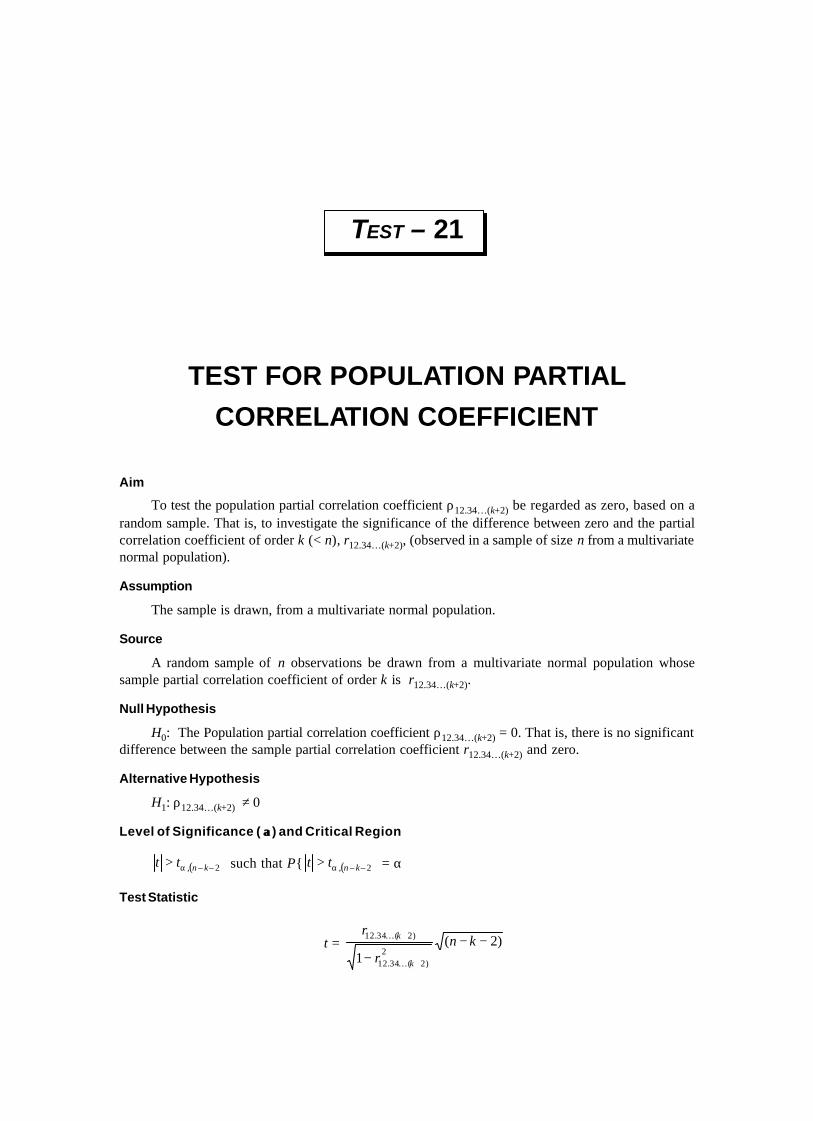
Aim
To test the population partial correlation coefficient ρ12.34…(k+2) be regarded as zero, based on arandom sample. That is, to investigate the significance of the difference between zero and the partialcorrelation coefficient of order k (< n), r12.34…(k+2), (observed in a sample of size n from a multivariatenormal population).
Assumption
The sample is drawn, from a multivariate normal population.
Source
A random sample of n observations be drawn from a multivariate normal population whosesample partial correlation coefficient of order k is r12.34…(k+2).
Null Hypothesis
H0: The Population partial correlation coefficient ρ12.34…(k+2) = 0. That is, there is no significantdifference between the sample partial correlation coefficient r12.34…(k+2) and zero.
Alternative Hypothesis
H1: ρ12.34…(k+2) ≠ 0
Level of Significance ( αα) and Critical Region
( )2––, kntt α> such that P{ ( )2––, kntt α> = α
Test Statistic
t = )2(1 2
)2.. .(34.12
)2. . .(34.12 −−− +
+ knr
r
k
k
TEST FOR POPULATION PARTIAL
CORRELATION COEFFICIENT
TEST – 21
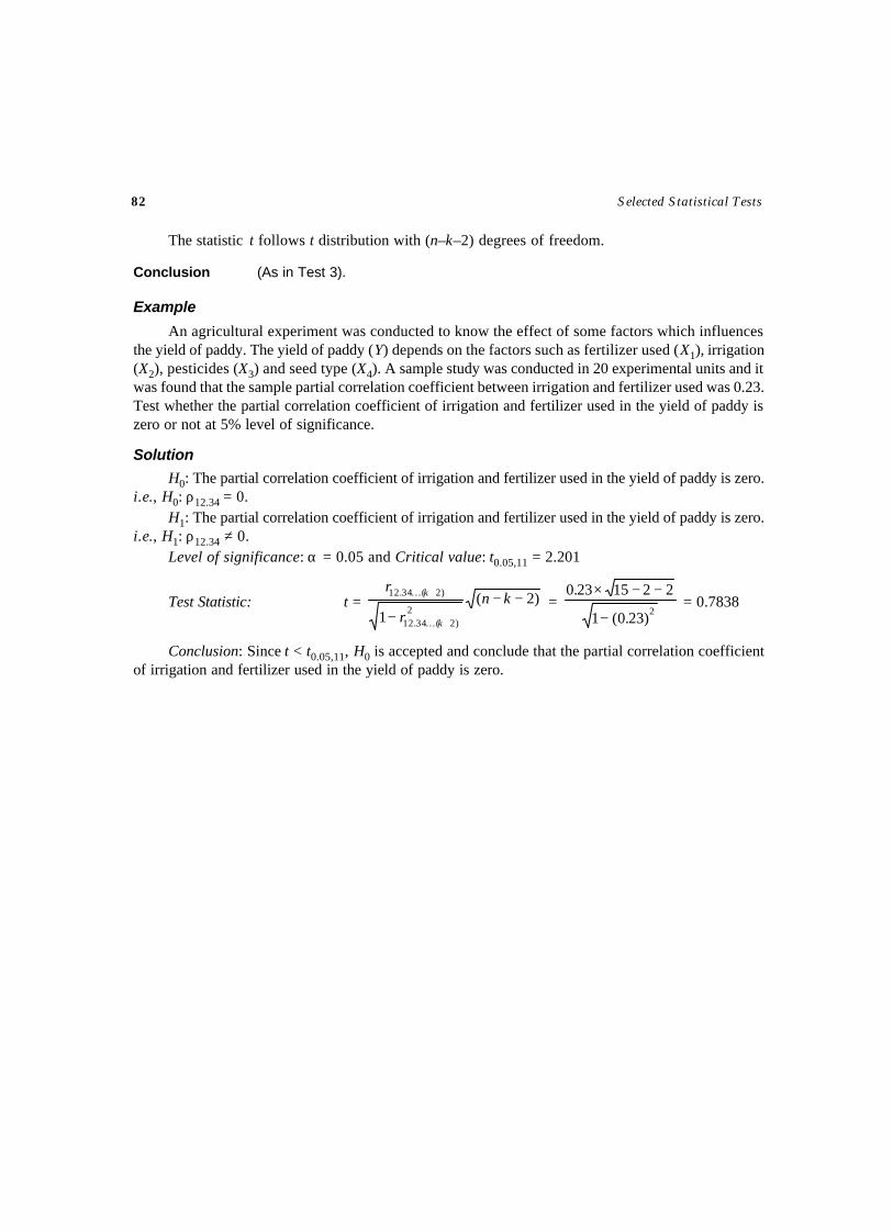
82 Selected Statistical Tests
The statistic t follows t distribution with (n–k–2) degrees of freedom.
Conclusion (As in Test 3).
Example
An agricultural experiment was conducted to know the effect of some factors which influencesthe yield of paddy. The yield of paddy (Y) depends on the factors such as fertilizer used (X1), irrigation(X2), pesticides (X3) and seed type (X4). A sample study was conducted in 20 experimental units and itwas found that the sample partial correlation coefficient between irrigation and fertilizer used was 0.23.Test whether the partial correlation coefficient of irrigation and fertilizer used in the yield of paddy iszero or not at 5% level of significance.
Solution
H0: The partial correlation coefficient of irrigation and fertilizer used in the yield of paddy is zero.i.e., H0: ρ12.34 = 0.
H1: The partial correlation coefficient of irrigation and fertilizer used in the yield of paddy is zero.i.e., H1: ρ12.34 ≠ 0.
Level of significance: α = 0.05 and Critical value: t0.05,11 = 2.201
Test Statistic: t = )2(1 2
)2.. .(34.12
)2. . .(34.12 −−− +
+ knr
r
k
k =
2)23.0(1
221523.0
−
−−× = 0.7838
Conclusion: Since t < t0.05,11, H0 is accepted and conclude that the partial correlation coefficientof irrigation and fertilizer used in the yield of paddy is zero.
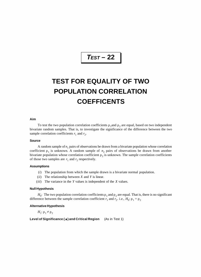
Aim
To test the two population correlation coefficients ρ1and ρ2 are equal, based on two independentbivariate random samples. That is, to investigate the significance of the difference between the twosample correlation coefficients r1 and r2.
Source
A random sample of n1 pairs of observations be drawn from a bivariate population whose correlationcoefficient ρ1 is unknown. A random sample of n2 pairs of observations be drawn from anotherbivariate population whose correlation coefficient ρ2 is unknown. The sample correlation coefficientsof those two samples are r1 and r2 respectively.
Assumptions
(i) The population from which the sample drawn is a bivariate normal population.(ii) The relationship between X and Y is linear.
(iii) The variance in the Y values is independent of the X values.
Null Hypothesis
H0: The two population correlation coefficients ρ1 and ρ2 are equal. That is, there is no significantdifference between the sample correlation coefficient r1 and r2. i.e., H0: ρ1 = ρ2
Alternative Hypothesis
H1: ρ1 ≠ ρ2
Level of Significance ( αα) and Critical Region (As in Test 1)
TEST FOR EQUALITY OF TWO
POPULATION CORRELATION
COEFFICENTS
TEST – 22
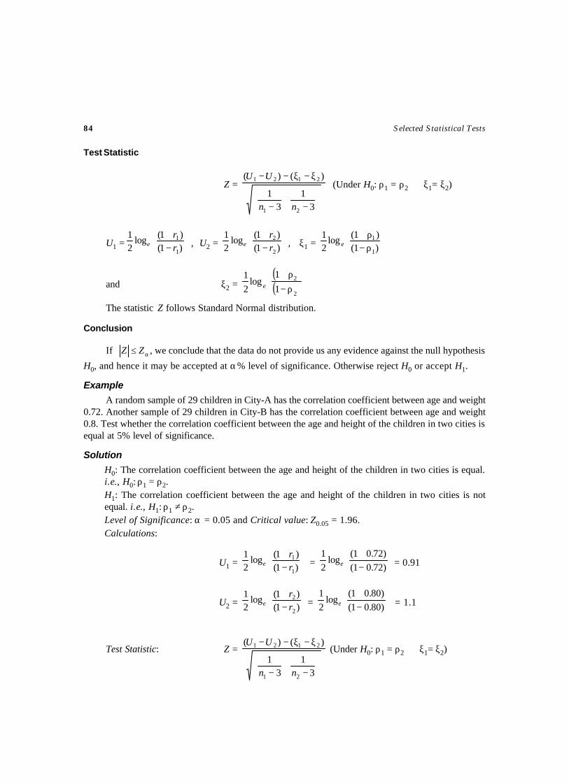
84 Selected Statistical Tests
Test Statistic
Z =
−+
−
ξ−ξ−−
31
31
)()(
21
2121
nn
UU (Under H0: ρ1 = ρ2 ⇒ ξ1= ξ2)
U1 =
−+
)1()1(log
21
1
1
rr
e , U2 =
−+
)1()1(log
21
2
2
rr
e , ξ1 =
ρ−ρ+
)1()1(log
21
1
1e
and ξ2 =( )( )
ρ−ρ+
2
2
1
1log
21
e
The statistic Z follows Standard Normal distribution.
Conclusion
If ,α≤ ZZ we conclude that the data do not provide us any evidence against the null hypothesis
H0, and hence it may be accepted at α% level of significance. Otherwise reject H0 or accept H1.
Example
A random sample of 29 children in City-A has the correlation coefficient between age and weight0.72. Another sample of 29 children in City-B has the correlation coefficient between age and weight0.8. Test whether the correlation coefficient between the age and height of the children in two cities isequal at 5% level of significance.
Solution
H0: The correlation coefficient between the age and height of the children in two cities is equal.i.e., H0: ρ1 = ρ2.H1: The correlation coefficient between the age and height of the children in two cities is notequal. i.e., H1: ρ1 ≠ ρ2.Level of Significance: α = 0.05 and Critical value: Z0.05 = 1.96.Calculations:
U1 =
−+
)1()1(log
21
1
1
rr
e =
−+
)72.01()72.01(
log21
e = 0.91
U2 =
−+
)1()1(log
21
2
2
rr
e =
−+
)80.01()80.01(
log21
e = 1.1
Test Statistic: Z =
−+
−
ξ−ξ−−
31
31
)()(
21
2121
nn
UU (Under H0: ρ1 = ρ2 ⇒ ξ1= ξ2)
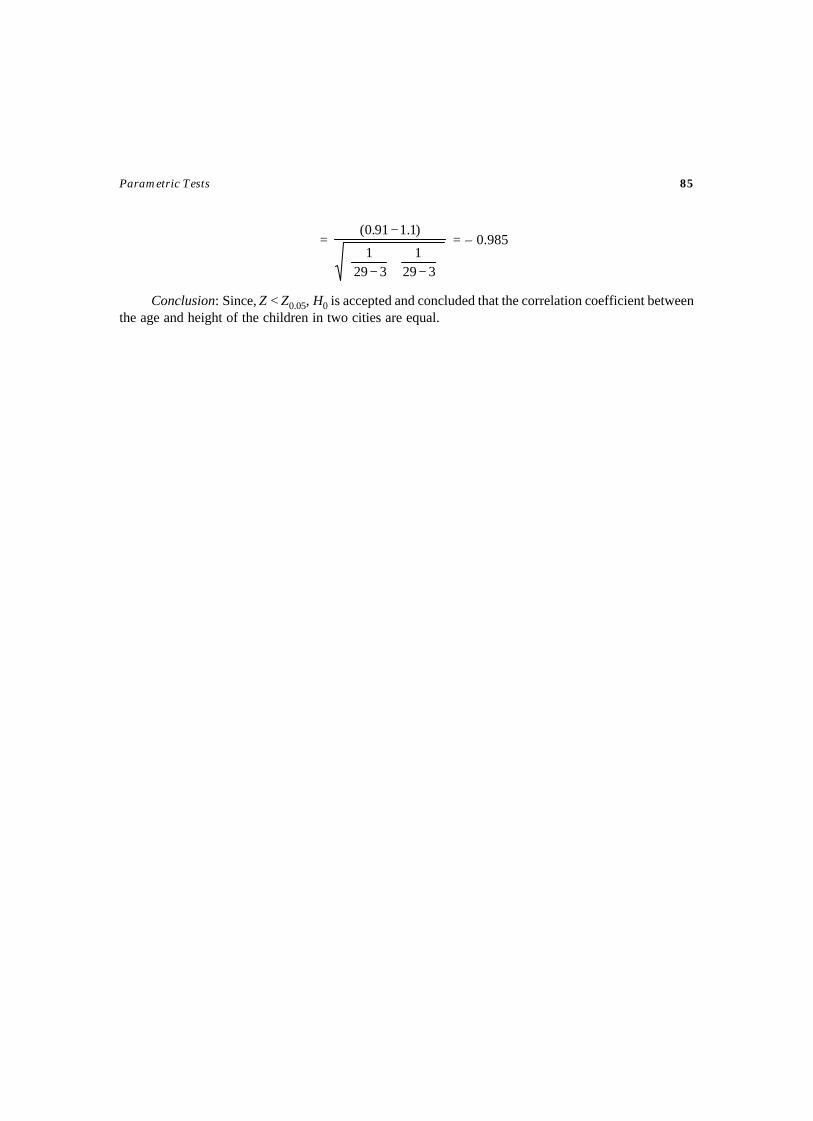
Parametric Tests 85
=
−+
−
−
3291
3291
)1.191.0( = – 0.985
Conclusion: Since, Z < Z0.05, H0 is accepted and concluded that the correlation coefficient betweenthe age and height of the children in two cities are equal.
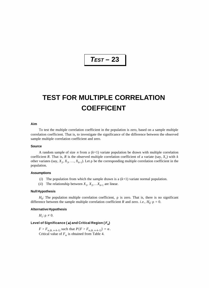
Aim
To test the multiple correlation coefficient in the population is zero, based on a sample multiplecorrelation coefficient. That is, to investigate the significance of the difference between the observedsample multiple correlation coefficient and zero.
Source
A random sample of size n from a (k+1) variate population be drawn with multiple correlationcoefficient R. That is, R is the observed multiple correlation coefficient of a variate (say, X1) with kother variates (say, X2, X3, …, Xk+1). Let ρ be the corresponding multiple correlation coefficient in thepopulation.
Assumptions
(i) The population from which the sample drawn is a (k+1) variate normal population.(ii) The relationship between X1, X2,…Xk+1 are linear.
Null Hypothesis
H0: The population multiple correlation coefficient, ρ is zero. That is, there is no significantdifference between the sample multiple correlation coefficient R and zero. i.e., H0: ρ = 0.
Alternative Hypothesis
H1: ρ ≠ 0.
Level of Significance ( αα) and Critical Region ( Fαα)
F > Fα,(k, n–k–1) such that P{F > Fα,(k, n–k–1)} = α.Critical value of Fα is obtained from Table 4.
TEST FOR MULTIPLE CORRELATION
COEFFICENT
TEST – 23
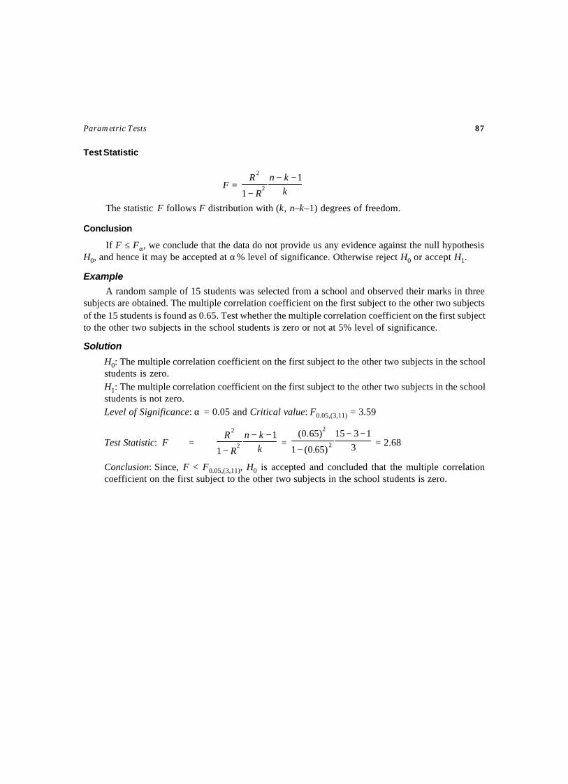
Parametric Tests 87
Test Statistic
F =kkn
R
R 1
12
2 −−
−The statistic F follows F distribution with (k, n–k–1) degrees of freedom.
Conclusion
If F ≤ Fα, we conclude that the data do not provide us any evidence against the null hypothesisH0, and hence it may be accepted at α% level of significance. Otherwise reject H0 or accept H1.
Example
A random sample of 15 students was selected from a school and observed their marks in threesubjects are obtained. The multiple correlation coefficient on the first subject to the other two subjectsof the 15 students is found as 0.65. Test whether the multiple correlation coefficient on the first subjectto the other two subjects in the school students is zero or not at 5% level of significance.
Solution
H0: The multiple correlation coefficient on the first subject to the other two subjects in the schoolstudents is zero.H1: The multiple correlation coefficient on the first subject to the other two subjects in the schoolstudents is not zero.Level of Significance: α = 0.05 and Critical value: F0.05,(3,11) = 3.59
Test Statistic: F =kkn
R
R 1
12
2 −−
− = 3
1315
)65.0(1
)65.0(2
2 −−
− = 2.68
Conclusion: Since, F < F0.05,(3,11), H0 is accepted and concluded that the multiple correlationcoefficient on the first subject to the other two subjects in the school students is zero.
Aim
To test the population regression coefficient of Y on X denoted by β be regarded as zero, basedon a bivariate random sample. That is, to investigate the significance of the difference between thesample regression coefficient of Y on X, b and zero.
Source
Let (Xi, Yi), ( i = 1, 2, …, n) be a random sample of n pairs of observations drawn from abivariate normal population whose regression coefficient of Y on X is β. The sample regression coefficientof Y on X is denoted by b.
Assumptions
(i) The population from which, the sample drawn, is a bivariate normal population.(ii) The relationship between X and Y is linear.
Null Hypothesis
H0: The population regression coefficient of Y on X, β is zero. That is, there is no significantdifference between the sample regression coefficient of Y on X, b and zero. i.e., H0: β = 0.
Alternative Hypothesis
H1: β ≠ 0
Level of Significance ( αα) and Critical Region
|t| > tα,(n–2) such that P{| t| > tα,(n–2)} = α
TEST FOR REGRESSION COEFFICIENT
TEST – 24
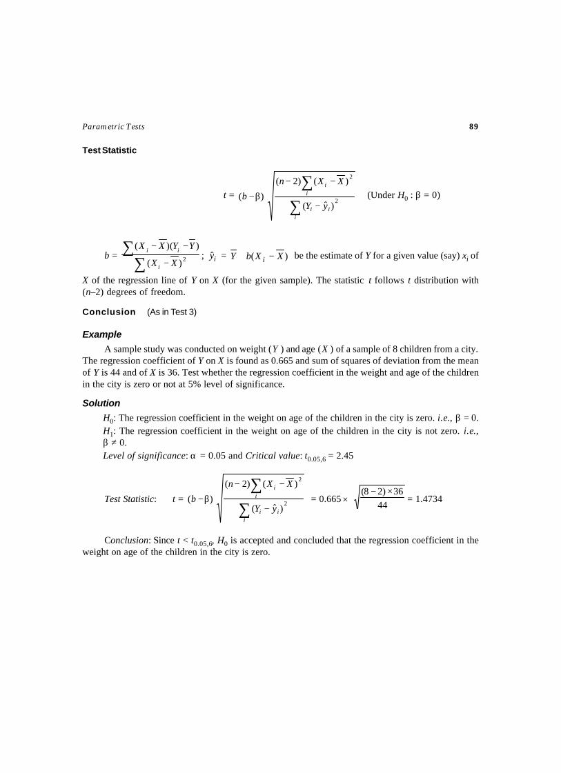
Parametric Tests 89
Test Statistic
t =
−
−−
β−∑
∑
iii
ii
yY
XXn
b 2
2
)ˆ(
)()2(
)( (Under H0 : β = 0)
b = ∑
∑−
−−2)(
))((
XX
YYXX
i
ii; iy = )( XXbY i −+ be the estimate of Y for a given value (say) xi of
X of the regression line of Y on X (for the given sample). The statistic t follows t distribution with(n–2) degrees of freedom.
Conclusion (As in Test 3)
Example
A sample study was conducted on weight (Y ) and age (X ) of a sample of 8 children from a city.The regression coefficient of Y on X is found as 0.665 and sum of squares of deviation from the meanof Y is 44 and of X is 36. Test whether the regression coefficient in the weight and age of the childrenin the city is zero or not at 5% level of significance.
Solution
H0: The regression coefficient in the weight on age of the children in the city is zero. i.e., β = 0.H1: The regression coefficient in the weight on age of the children in the city is not zero. i.e.,β ≠ 0.Level of significance: α = 0.05 and Critical value: t0.05,6 = 2.45
Test Statistic: t =
−
−−
β−∑
∑
iii
ii
yY
XXn
b 2
2
)ˆ(
)()2(
)( = 0.665 × 44
36)28( ×−= 1.4734
Conclusion: Since t < t0.05,6, H0 is accepted and concluded that the regression coefficient in theweight on age of the children in the city is zero.
Aim
To test the regression that passes through the origin. That is, to investigate the significance of thedifference between the intercept of a regression and zero.
Source
A random sample of size n from a bivariate population be drawn. The intercept of the regressionin the population is denoted by α . The regression with α = 0 is known as regression through origin.The linear regression in the sample is y = a + bx, where a is the intercept and b is the slope of the linearregression.
Assumptions
(i) The population from which, the sample drawn is a bi-variate normal population.(ii) The relationship between Y and X are linear.
Null Hypothesis
H0: The intercept of the regression in the population is zero. That is, there is no significantdifference between the intercept of the linear regression in the sample and zero. i.e., H0: α = 0.
Alternative Hypothesis
H1: α ≠ 0.
Level of Significance ( αα) and Critical Region ( t αα)
t > tα,(n–2) such that P {t > tα,(n–2)} = α .
Critical value of tα is obtained from Table 2.
TEST FOR INTERCEPT IN A REGRESSION
TEST – 25

Parametric Tests 91
Method
For the given bivariate data with Y is the dependent variable and X is the independent variable onn observations, calculate the following:
(i) ∑ y ;2∑ y ; ∑ x ;
2∑ x ; yx∑ ; x and y .
(ii) Sum of Squares of the observations y = SS(Y) = .–
2
2∑∑
n
yy
(iii) Sum of Squares of the observations x = SS(X) = .–
2
2∑∑
n
xx
(iv) Sum of Products of the observations x and y = SP(XY) = .–∑ ∑∑n
yxxy
(v) The regression coefficient, b = ( )( ) .XSS
XYSP
(vi) The intercept of the regression, a = xby – .
(vii) Sum of Squares due to regression b = SS(b) = ( )[ ]
( ) .2
XSSXYSP
(viii) ESS = SS(Y) – SS(b).
(ix) Error Mean Square, 2es = .
1–nESS
Test Statistic
t =( )
+
−
)(1
02
2
XSSx
ns
a
e
The statistic t follows t distribution with (n–2) degrees of freedom.
Conclusion
If α≤ tt , we conclude that the data do not provide us any evidence against the null hypothesis
H0, and hence it may be accepted at α% level of significance. Otherwise reject H0 or accept H1.
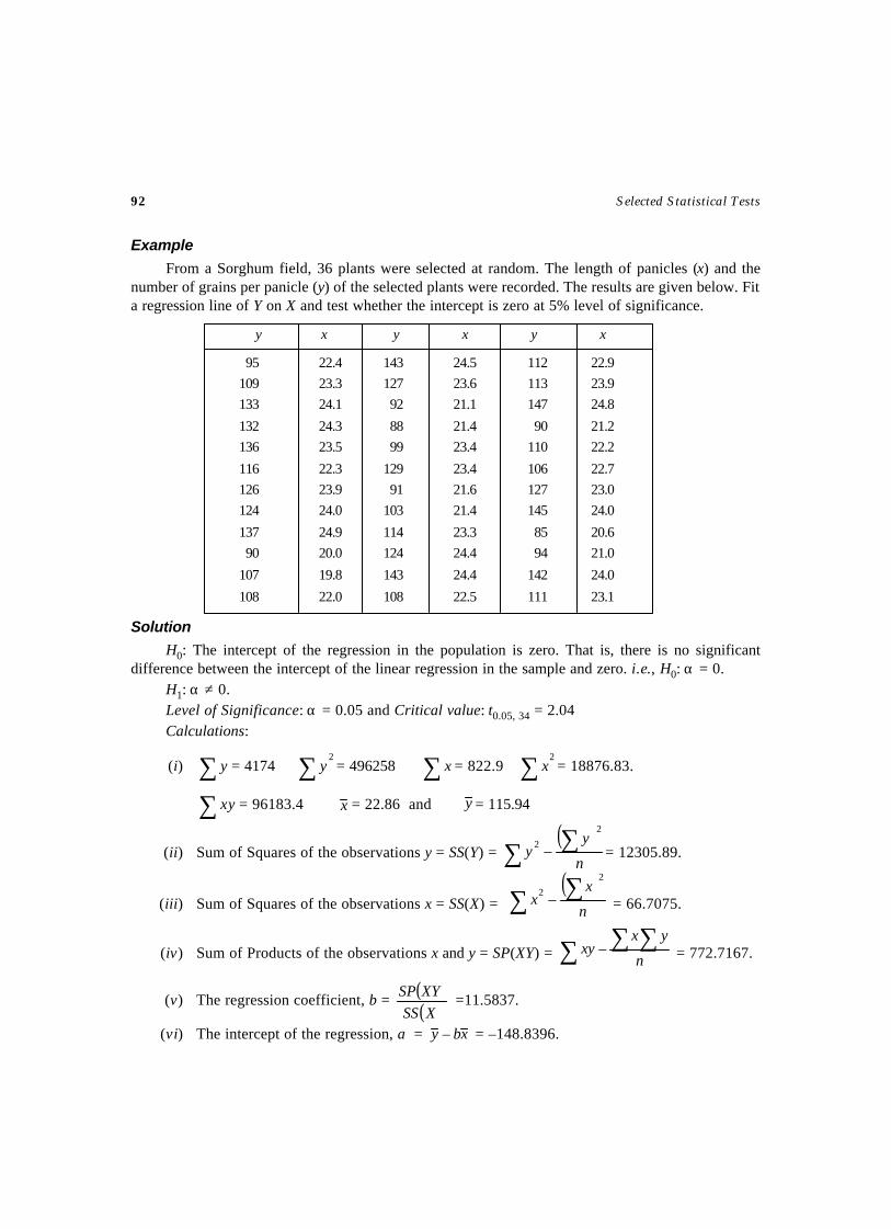
92 Selected Statistical Tests
Example
From a Sorghum field, 36 plants were selected at random. The length of panicles (x) and thenumber of grains per panicle (y) of the selected plants were recorded. The results are given below. Fita regression line of Y on X and test whether the intercept is zero at 5% level of significance.
y x y x y x
95 22.4 143 24.5 112 22.9
109 23.3 127 23.6 113 23.9
133 24.1 92 21.1 147 24.8
132 24.3 88 21.4 90 21.2
136 23.5 99 23.4 110 22.2
116 22.3 129 23.4 106 22.7
126 23.9 91 21.6 127 23.0
124 24.0 103 21.4 145 24.0
137 24.9 114 23.3 85 20.6
90 20.0 124 24.4 94 21.0
107 19.8 143 24.4 142 24.0
108 22.0 108 22.5 111 23.1
Solution
H0: The intercept of the regression in the population is zero. That is, there is no significantdifference between the intercept of the linear regression in the sample and zero. i.e., H0: α = 0.
H1: α ≠ 0.Level of Significance: α = 0.05 and Critical value: t0.05, 34 = 2.04Calculations:
(i) ∑ y = 41742∑ y = 496258 ∑ x = 822.9
2∑ x = 18876.83.
yx∑ = 96183.4 x = 22.86 and y = 115.94
(ii) Sum of Squares of the observations y = SS(Y) = ( )
∑ ∑n
yy
2
2 – = 12305.89.
(iii) Sum of Squares of the observations x = SS(X) = ( )
∑ ∑n
xx
2
2 – = 66.7075.
(iv) Sum of Products of the observations x and y = SP(XY) = ∑ ∑∑n
yxxy – = 772.7167.
(v) The regression coefficient, b = ( )( )XSSXYSP =11.5837.
(vi) The intercept of the regression, a = xby – = –148.8396.
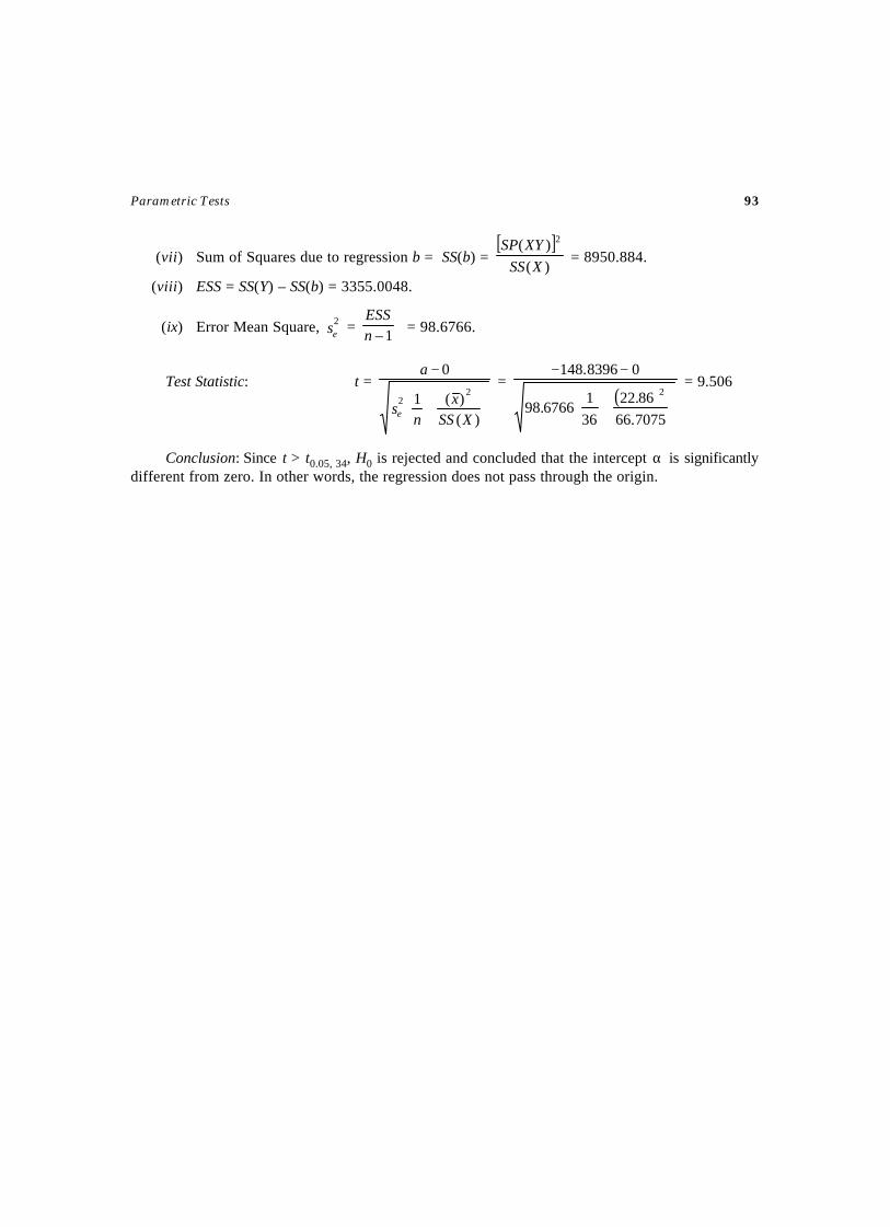
Parametric Tests 93
(vii) Sum of Squares due to regression b = SS(b) = [ ]
)()( 2
XSSXYSP
= 8950.884.
(viii) ESS = SS(Y) – SS(b) = 3355.0048.
(ix) Error Mean Square, 2es = 1–n
ESS = 98.6766.
Test Statistic: t =
+
−
)()(1
02
2
XSSx
ns
a
e
= ( )
+
−−
7075.6686.22
361
6766.98
08396.1482
= 9.506
Conclusion: Since t > t0.05, 34, H0 is rejected and concluded that the intercept α is significantlydifferent from zero. In other words, the regression does not pass through the origin.

This pageintentionally left
blank

ANALYSIS OF VARIANCE TESTS
CHAPTER – 3

This pageintentionally left
blank

Aim
To test the significance of the t treatment effects based on the observations from n experimentalunits.
Source
Let yij, (i = 1, 2,…, t; j = 1, 2,…, r) be the observations of t treatments, each replicated with(equal number of replications) r times in n experimental units (i.e., n = tr). In this design, treatmentsare allocated at random to the experimental units over the entire experimental material. That is, theentire experimental material is divided into n experimental units and the treatments are distributedcompletely at random over the units.
Linear Model
The linear model is yij = µ + τi + εij ; (i = 1, 2,…, t; j = 1, 2,…, r),where yij is the observation from the jth replication of the ith treatment, µ is the overall mean effect, τiis the effect due to the ith treatment and εij is the error effect due to chance causes.
Assumptions
(i) The population from which, the observations drawn is Normal distribution.(ii) The observations are independent.
(iii) The various effects are additive in nature.(iv) εij are identically independently distributed as Normal distribution with mean zero and variance
2εσ .
Null Hypothesis
H0: The k treatments have equal effect. i.e., H0: τ1 = τ2 = … = τt.
TEST FOR COMPLETELY RANDOMIZED
DESIGN
TEST – 26
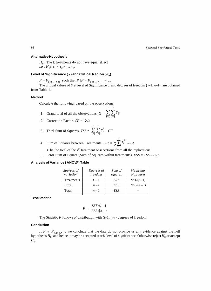
98 Selected Statistical Tests
Alternative Hypothesis
H1: The k treatments do not have equal effecti.e., H1: τ1 ≠ τ2 ≠ … ττ.
Level of Significance ( αα) and Critical Region ( Fαα)
F > Fα,(t–1, n-t) such that P [F > Fα,(t–1, n–t)] = α .The critical values of F at level of Significance α and degrees of freedom (t–1, n–1), are obtained
from Table 4.
Method
Calculate the following, based on the observations:
1. Grand total of all the observations, G = ∑∑= =
t
i
r
jijy
1 1
2. Correction Factor, CF = G2/n
3. Total Sum of Squares, TSS = ∑∑= =
t
i
r
jijy
1 1
2
– CF
4. Sum of Squares between Treatments, SST = ∑=
t
iiT
r 1
21 – CF
Ti be the total of the ith treatment observations from all the replications.5. Error Sum of Square (Sum of Squares within treatments), ESS = TSS – SST
Analysis of Variance ( ANOVA) Table
Sources of Degrees of Sum of Mean sumvariation freedom squares of squares
Treatments t – 1 SST SST/(t – 1)
Error n – t ESS ESS/(n – t)
Total n – 1 TSS –
Test Statistic
F = ( )( )tnESStSST
–/–/ 1
The Statistic F follows F distribution with (t–1, n–t) degrees of freedom.
Conclusion
If F ≤ Fα,(t–1,n–t), we conclude that the data do not provide us any evidence against the nullhypothesis H0, and hence it may be accepted at α% level of significance. Otherwise reject H0 or acceptH1.
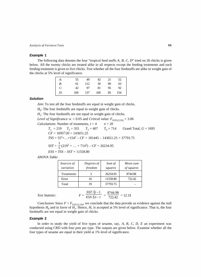
Analysis of Variance Tests 99
Example 1
The following data denotes the four “tropical feed stuffs A, B, C, D” tried on 20 chicks is givenbelow. All the twenty chicks are treated alike in all respects except the feeding treatments and eachfeeding treatment is given to five chicks. Test whether all the four feedstuffs are alike in weight gain ofthe chicks at 5% level of significance.
A: 55 49 42 21 52B: 61 112 30 89 63C: 42 97 81 95 92
D: 169 137 169 85 154
Solution
Aim: To test all the four feedstuffs are equal in weight gain of chicks.H0: The four feedstuffs are equal in weight gain of chicks.H1: The four feedstuffs are not equal in weight gain of chicks.Level of Significance: α = 0.05 and Critical value: F0.05,(3,16) = 3.06Calculations: Number of treatments, t = 4 n = 20
T1 = 219 T2 = 355 T3 = 407 T4 = 714 Grand Total, G = 1695CF = 16952/20 = 143651.25TSS = 552+…+1542 – CF = 181445 – 143651.25 = 37793.75
SST = 51
(2192 + … + 7142) – CF = 26234.95
ESS = TSS – SST = 11558.80
ANOVA Table:
Sources of Degrees of Sum of Mean sumvariation freedom squares of squares
Treatments 3 26234.95 8744.98
Error 16 11558.80 722.42
Total 19 37793.75 –
Test Statistic: F =( )( )tnESStSST
–/1–/
= 42.72298.8744
= 12.111
Conclusion: Since F > F0.05,(3,16), we conclude that the data provide us evidence against the nullhypothesis H0 and in favor of H1. Hence, H1 is accepted at 5% level of significance. That is, the fourfeedstuffs are not equal in weight gain of chicks.
Example 2
In order to study the yield of five types of sesame, say, A, B, C, D, E an experiment wasconducted using CRD with four pots per type. The outputs are given below. Examine whether all thefour types of sesame are equal in their yield at 1% level of significance.
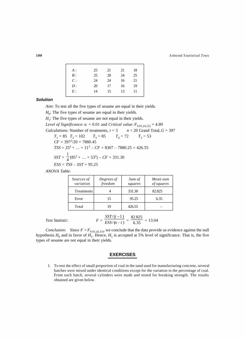
100 Selected Statistical Tests
A : 25 21 21 18B : 25 28 24 25C : 24 24 16 21D : 20 17 16 19E : 14 15 13 11
Solution
Aim: To test all the five types of sesame are equal in their yields.H0: The five types of sesame are equal in their yields.H1: The five types of sesame are not equal in their yields.Level of Significance: α = 0.01 and Critical value: F0.01,(4,15) = 4.89Calculations: Number of treatments, t = 5 n = 20 Grand Total, G = 397
T1 = 85 T2 = 102 T3 = 85 T4 = 72 T5 = 53CF = 3972/20 = 7880.45TSS = 252 + … + 112 – CF = 8307 – 7880.25 = 426.55
SST = 41
(852 + … + 532) – CF = 331.30
ESS = TSS – SST = 95.25
ANOVA Table:
Sources of Degrees of Sum of Mean sumvariation freedom squares of squares
Treatments 4 331.30 82.825
Error 15 95.25 6.35
Total 19 426.55 –
Test Statistic: F = )–(/)1–(/
tnESStSST
= 35.6825.82
= 13.04
Conclusion: Since F > F0.01,(4,15), we conclude that the data provide us evidence against the nullhypothesis H0 and in favor of H1. Hence, H1 is accepted at 5% level of significance. That is, the fivetypes of sesame are not equal in their yields.
EXERCISES
1. To test the effect of small proportion of coal in the sand used for manufacturing concrete, severalbatches were mixed under identical conditions except for the variation in the percentage of coal.From each batch, several cylinders were made and tested for breaking strength. The resultsobtained are given below.
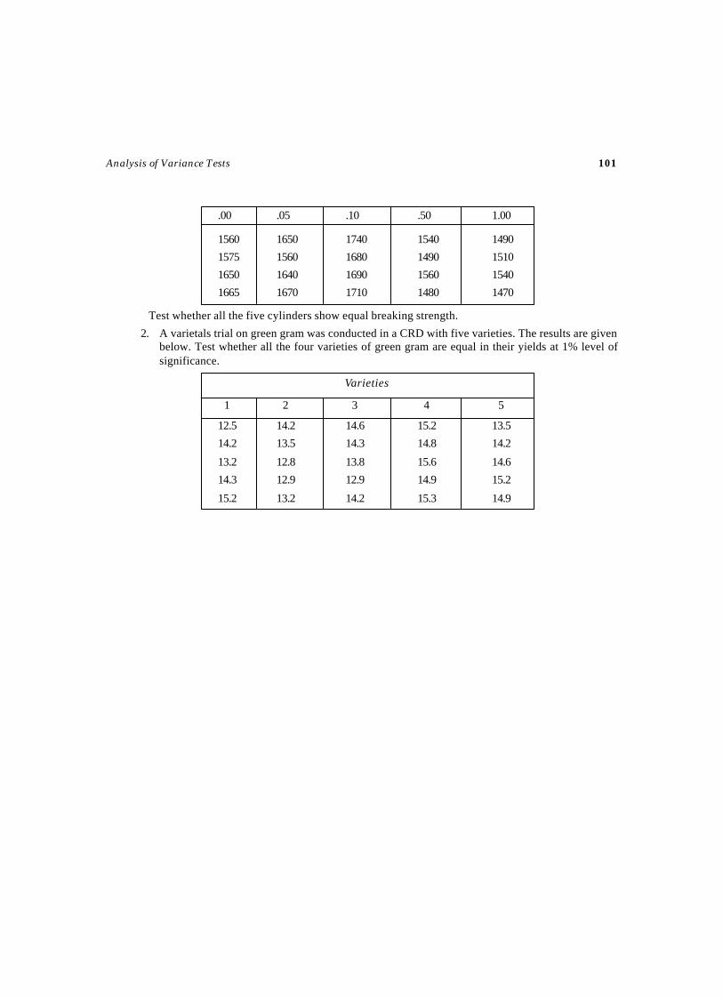
Analysis of Variance Tests 101
.00 .05 .10 .50 1.00
1560 1650 1740 1540 1490
1575 1560 1680 1490 1510
1650 1640 1690 1560 1540
1665 1670 1710 1480 1470
Test whether all the five cylinders show equal breaking strength.
2. A varietals trial on green gram was conducted in a CRD with five varieties. The results are givenbelow. Test whether all the four varieties of green gram are equal in their yields at 1% level ofsignificance.
Varieties
1 2 3 4 5
12.5 14.2 14.6 15.2 13.5
14.2 13.5 14.3 14.8 14.2
13.2 12.8 13.8 15.6 14.6
14.3 12.9 12.9 14.9 15.2
15.2 13.2 14.2 15.3 14.9

Aim
To test the significance of the treatment effects and the significance of the regression coefficientof Y on X, based on the observations from n experimental units.
Source
Let (Yij, Xij) ( i = 1, 2,…, t; j = 1, 2,…, r) be the observations made from an experiment consistsof t treatments each with replicated r times on two variables Y and X. The observations on auxiliary orconcomitant variable, X apart from the main variable Y under study is available for each of theexperimental units. When Y and X are associated, a part of the variation of Y is due to variation in valuesof X. After eliminating, the effects of blocks and treatments one can then estimate a relationship,between Y and X and use that relationship to predict the value of Y for a given value of X. This test isused for assessing the significance of relationship between X and Y. If there is, a significant associationbetween X and Y one may calculate the adjusted treatment sum of squares and perform the test for thehomogeneity of treatment effects. Let n = t × r. The observed data is arranged as follows:
Treatments1 2 … T
Y X Y X … Y XY11 X11 Y21 X21 … Yt1 Xt1
Y12 X12 Y22 X22 … Yt2 Xt2
… … … … … … …
… … … … … … …… … … … … … …
Y1r X1r Y2r X2r … Ytr Xtr
Treatment totals
TY1 TX1 TY2 TX2 … TYt TXt
ANOCOVA TEST FOR COMPLETELY
RANDOMIZED DESIGN
TEST – 27
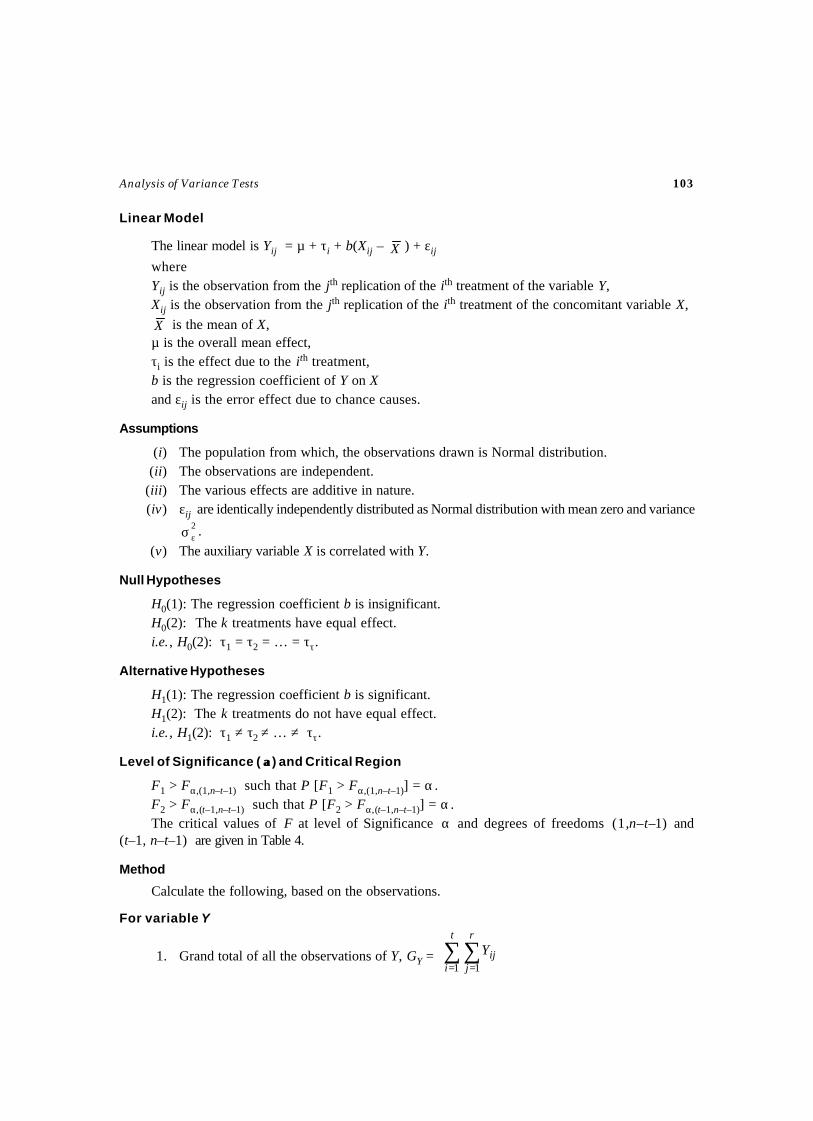
Analysis of Variance Tests 103
Linear Model
The linear model is Yij = µ + τi + b(Xij – X ) + εij
whereYij is the observation from the jth replication of the ith treatment of the variable Y,Xij is the observation from the jth replication of the ith treatment of the concomitant variable X,
X is the mean of X,µ is the overall mean effect,τi is the effect due to the ith treatment,b is the regression coefficient of Y on Xand εij is the error effect due to chance causes.
Assumptions
(i) The population from which, the observations drawn is Normal distribution.(ii) The observations are independent.
(iii) The various effects are additive in nature.(iv) εij are identically independently distributed as Normal distribution with mean zero and variance
2εσ .
(v) The auxiliary variable X is correlated with Y.
Null Hypotheses
H0(1): The regression coefficient b is insignificant.H0(2): The k treatments have equal effect.i.e., H0(2): τ1 = τ2 = … = ττ.
Alternative Hypotheses
H1(1): The regression coefficient b is significant.H1(2): The k treatments do not have equal effect.i.e., H1(2): τ1 ≠ τ2 ≠ … ≠ ττ.
Level of Significance ( αα) and Critical Region
F1 > Fα,(1,n–t–1) such that P [F1 > Fα,(1,n–t–1)] = α .F2 > Fα,(t–1,n–t–1) such that P [F2 > Fα,(t–1,n–t–1)] = α .The critical values of F at level of Significance α and degrees of freedoms (1,n–t–1) and
(t–1, n–t–1) are given in Table 4.
Method
Calculate the following, based on the observations.
For variable Y
1. Grand total of all the observations of Y, GY = ∑∑= =
t
i
r
jijY
1 1

104 Selected Statistical Tests
2. Correction Factor, CFY = n
GY2
.
3. Total Sum of Squares, GYY = ∑∑= =
t
i
r
jijY
1 1
2
– CFY
4. Treatment Sum of Squares, TYY = ∑=
t
iYiT
r 1
21– CFY
Tyi be the total of the ith treatment observations of Y.5. Error Sum of Squares, EYY = GYY – TYY
For variable X
6. Grand total of all the observations, GX = ∑∑= =
t
i
r
jijX
1 1
7. Correction Factor, CFX = n
GX2
8. Total Sum of Squares, GXX = ∑∑= =
t
i
r
jijX
1 1
2
– CFX
9. Treatment Sum of Squares, TXX = ∑=
t
iXiT
r 1
21 – CFX
TXi be the total of the ith treatment observations of X, from all the replications.10. Error Sum of Squares, EXX = GXX – TXX
For variables Y and X
11. Correction Factor, CFYX = n
GG XY ×
12. Total Sum of Products of Y and X, GYX = ∑∑= =
×t
i
r
jijij XY
1 1– CFYX
13. Treatment Sum of products of Y and X, TYX = ∑=
×t
iXiYi TT
r 1
1– CFYX
14. Error Sum of Products, EYX = GYX – TYX
15. The regression coefficient within treatment, b = EYX/ EXX
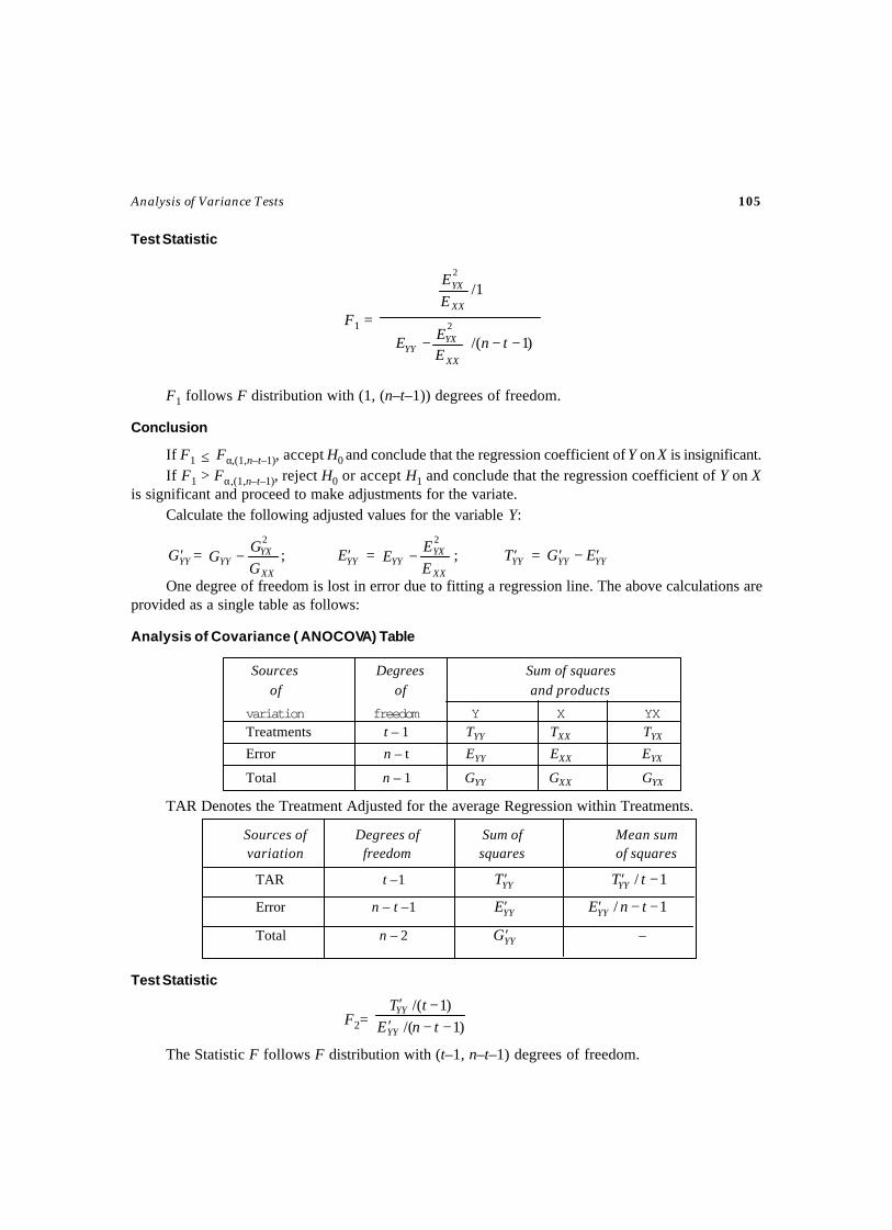
Analysis of Variance Tests 105
Test Statistic
F1 =
−−
−
)1/(
1/
2
2
tnEEE
EE
XX
YXYY
XX
YX
F1 follows F distribution with (1, (n–t–1)) degrees of freedom.
Conclusion
If F1 ≤ Fα,(1,n–t–1), accept H0 and conclude that the regression coefficient of Y on X is insignificant.If F1 > Fα,(1,n–t–1), reject H0 or accept H1 and conclude that the regression coefficient of Y on X
is significant and proceed to make adjustments for the variate.Calculate the following adjusted values for the variable Y:
YYG′ = XX
YXYY G
GG
2
− ; YYE′ = XX
YXYY E
EE
2
− ; YYT ′ = YYYY EG ′−′
One degree of freedom is lost in error due to fitting a regression line. The above calculations areprovided as a single table as follows:
Analysis of Covariance ( ANOCOVA) Table
Sources Degrees Sum of squaresof of and products
variation freedom Y X YXTreatments t – 1 TYY TXX TYX
Error n – t EYY EXX EYX
Total n – 1 GYY GXX GYX
TAR Denotes the Treatment Adjusted for the average Regression within Treatments.
Sources of Degrees of Sum of Mean sumvariation freedom squares of squares
TAR t –1 YYT ′ 1/ −′ tTYY
Error n – t –1 YYE′ 1/ −−′ tnEYY
Total n – 2 YYG′ –
Test Statistic
F2= )1/()1/(−−′
−′tnE
tT
YY
YY
The Statistic F follows F distribution with (t–1, n–t–1) degrees of freedom.

106 Selected Statistical Tests
Conclusion
If F2 ≤ Fα, (t–1, n–t–1), we conclude that the data do not provide us any evidence against the nullhypothesis H0(2), and hence it may be accepted at α% level of significance. Otherwise reject H0(2) oraccept H1(2).
Example
The following data shows the age, X (in months) and weight, Y (in kgs) of samples of childrenfrom three states namely Tamilnadu (A), Kerala (B) and Karnataka (C). Test whether the regressioncoefficient of Y on X is significant and the children from all the three states are homogeneous.
A B C
Y X Y X Y X
7.25 9 10.5 10 8.5 88.65 10 12.5 11 12.5 9
12.5 12 7.5 6 18.5 1515.5 14 15.5 12 16.5 13
16.5 15 16.5 14 13.5 10
Solution
H0(1): The regression coefficient of weight on age, b is insignificant.H0(2): The children from the three states are homogeneous.H1(1): The regression coefficient of weight on age, b is significant.H1(2): The children from the three states are not homogeneous.Level of Significance: α = 0.05Critical Values: F0.05,(1,11) = 4.84 and F0.05,(2,11) =3.98Calculations:
For variable Y
1. GY = 192.4; 2. CFY = n
GY2
= 2467.85
3. GYY = ∑∑= =
t
i
r
jijY
1 1
2
– CFY = 2660.3225 – 2467.85 = 192.4725
4. TYY = ∑=
t
iYiT
r 1
21– CFY = 2476.932 – 2467.85 = 9.082
5. EYY = GYY – TYY = 192.4725 – 9.082 = 183.3905
For variable X
6. GX = ∑∑= =
t
i
r
jijX
1 1 = 168; 7. CFX =
nGX
2
= 1881.6

Analysis of Variance Tests 107
8. GXX = ∑∑= =
t
i
r
jijX
1 1
2
– CFX = 1982 – 1881.6 = 100.4
9. TXX = ∑=
t
iXiT
r 1
21 – CFX = 1886.8 – 1881.6 = 5.2
10. EXX = GXX – TXX = 100.4 – 5.2 = 95.2
For variables Y and X
11. CFYX = n
GG XY × = 2154.88
12. GYX = ∑∑= =
×t
i
r
jijij XY
1 1 – CFYX = 2278.25 – 2154.88 = 123.37
13. TYX = ∑=
×t
iXiYi TT
r 1
1 – CFYX = 2151.8 – 2154.88 = –3.08
14. EYX = GYX – TYX = 123.37 – (–3.08) = 126.45
15. b = EYX/EXX = 126.45/95.2 = 1.3283
Test Statistic: F1 =
−−
−
)1/(
1/
2
2
tnEEE
EE
XX
YXYY
XX
YX
= 11/)958.1673905.183(
2.95602.15989
− = 119.71
Conclusion: Since F1 > F0.05,(1,11), reject H0(1), accept H1(1) and conclude that the regressioncoefficient of Y on X is significant. That is, the regression coefficient of weight on age of the childrenis significant.
Calculate the following adjusted values for the variable Y
YYG′ = GYY – XX
YX
GG 2
= 192.4725 – 4.100
)37.123( 2
= 40.8773
YYE′ = XX
YXYY E
EE
2
− = 183.3905 – 2.95
)45.126( 2
= 15.4325
YYT ′ = ''YYYY EG − = 40.9773 – 15.4325 = 25.4448
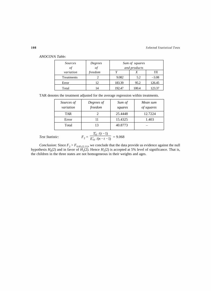
108 Selected Statistical Tests
ANOCOVA Table:
Sources Degrees Sum of squaresof of and products
variation freedom Y X YX
Treatments 2 9.082 5.2 –3.08
Error 12 183.39 95.2 126.45
Total 14 192.47 100.4 123.37
TAR denotes the treatment adjusted for the average regression within treatments.
Sources of Degrees of Sum of Mean sumvariation freedom squares of squares
TAR 2 25.4448 12.7224
Error 11 15.4325 1.403
Total 13 40.8773 –
Test Statistic: F2 = )1/()1/(−−′
−′tnE
tT
YY
YY = 9.068
Conclusion: Since F2 > F0.05,(2,11), we conclude that the data provide us evidence against the nullhypothesis H0(2) and in favor of H1(2). Hence H1(2) is accepted at 5% level of significance. That is,the children in the three states are not homogeneous in their weights and ages.

Aim
To test the significance of the t treatment effects and the significance of the r block effects basedon the observations from n experimental units.
Source
Let yij, ( i = 1, 2,…, t ; j = 1, 2,…, r) be the observations of k treatments, each applied with(equal number of replications) r times in n experimental units. In this design, the entire experimentalmaterial is divided into r homogeneous blocks, each block is further divided into t sub units such that t× r = n. The t treatments are allocated to each block randomly and for every r blocks. That is,randomization is restricted within blocks.
Linear Model
The linear model is yij = µ + τi + βj + εij ; ( i = 1, 2,…, t ; j = 1, 2, …, r)where yij is the observation from the jth block of the ith treatment, µ is the overall mean effect, τi is theeffect due to the ith treatment, βj is the effect due to the jth block and εij is the error effect due tochance causes.
Assumptions
(i) The population from which, the observations drawn is Normal distribution.(ii) The observations are independent.
(iii) The various effects are additive in nature.(iv) εij are identically independently distributed as Normal distribution with mean zero and variance
2εσ .
Null Hypotheses
H0(1): The k treatments have equal effect. i.e., H0: τ1 = τ2 = … = ττ.H0(2): The r blocks have equal effect. i.e., H0: β1 = β2 = … = βr.
TEST FOR RANDOMIZED BLOCK DESIGN
TEST – 28
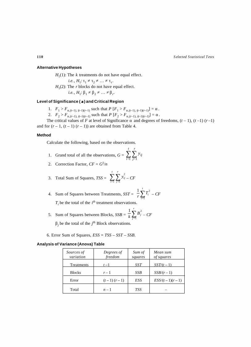
110 Selected Statistical Tests
Alternative Hypotheses
H1(1): The k treatments do not have equal effect.i.e., H1: τ1 ≠ τ2 ≠ … ≠ ττ.
H1(2): The r blocks do not have equal effect.i.e., H1: β1 ≠ β2 ≠ … ≠ βr.
Level of Significance ( αα) and Critical Region
1. F1 > Fα,(t–1), (t–1)(r–1) such that P [F1 > Fα,(t–1), (t–1)(r–1)] = α .2. F2 > Fα,(r–1), (t–1)(r–1) such that P [F2 > Fα,(r–1), (t–1)(r–1)] = α .
The critical values of F at level of Significance α and degrees of freedoms, (t – 1), (t –1) (r –1)and for (r – 1, (t – 1) (r – 1)) are obtained from Table 4.
Method
Calculate the following, based on the observations.
1. Grand total of all the observations, G = ∑∑= =
t
i
r
jijy
1 1
2. Correction Factor, CF = G2/n
3. Total Sum of Squares, TSS = ∑∑= =
t
i
r
jijy
1 1
2
– CF
4. Sum of Squares between Treatments, SST = ∑=
t
iiT
r 1
21– CF
Ti be the total of the ith treatment observations.
5. Sum of Squares between Blocks, SSB = ∑=
r
jjB
k 1
21– CF
βj be the total of the jth Block observations.
6. Error Sum of Squares, ESS = TSS – SST – SSB.
Analysis of Variance (Anova) Table
Sources of Degrees of Sum of Mean sumvariation freedom squares of squares
Treatments t –1 SST SST/(t – 1)
Blocks r – 1 SSB SSB/(r – 1)
Error (t – 1) (r – 1) ESS ESS/(t – 1)(r – 1)
Total n – 1 TSS –
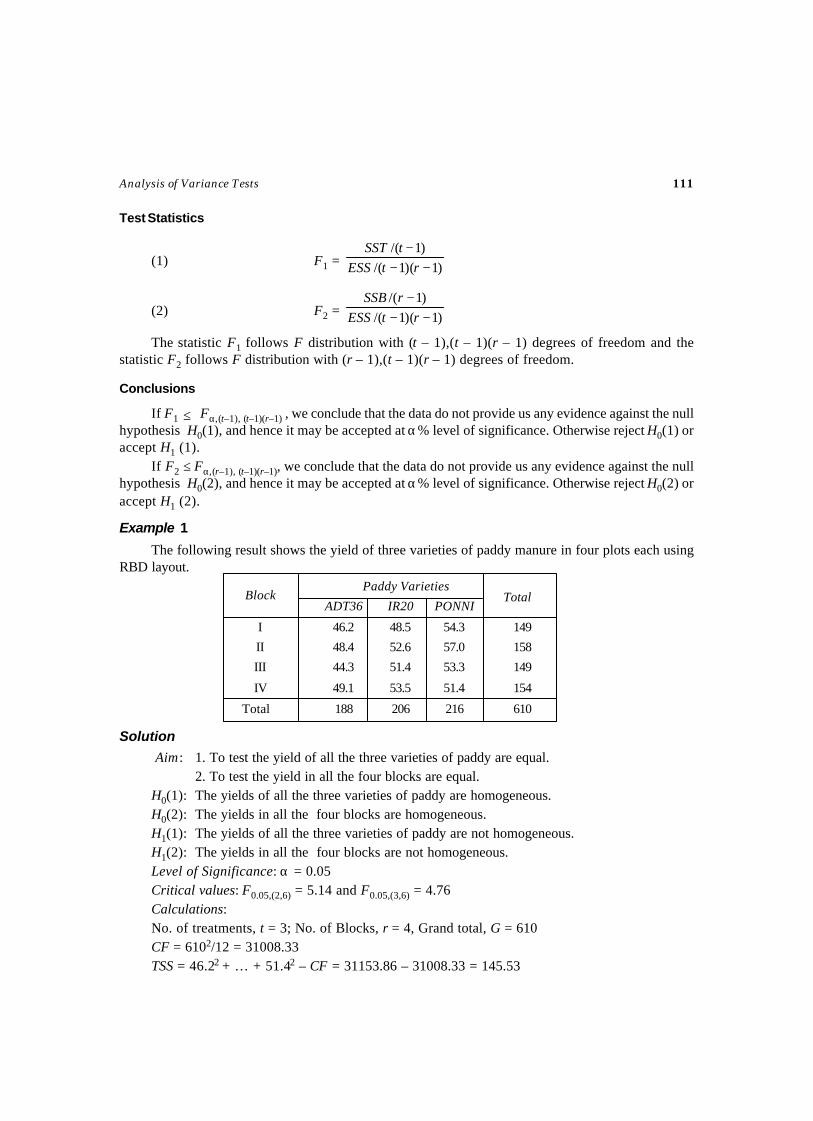
Analysis of Variance Tests 111
Test Statistics
(1) F1 = )1)(1/()1/(−−
−rtESS
tSST
(2) F2 = )1)(1/()1/(−−
−rtESS
rSSB
The statistic F1 follows F distribution with (t – 1),(t – 1)(r – 1) degrees of freedom and thestatistic F2 follows F distribution with (r – 1),(t – 1)(r – 1) degrees of freedom.
Conclusions
If F1 ≤ Fα,(t–1), (t–1)(r–1) , we conclude that the data do not provide us any evidence against the nullhypothesis H0(1), and hence it may be accepted at α% level of significance. Otherwise reject H0(1) oraccept H1 (1).
If F2 ≤ Fα,(r–1), (t–1)(r–1), we conclude that the data do not provide us any evidence against the nullhypothesis H0(2), and hence it may be accepted at α% level of significance. Otherwise reject H0(2) oraccept H1 (2).
Example 1
The following result shows the yield of three varieties of paddy manure in four plots each usingRBD layout.
Paddy Varieties
ADT36 IR20 PONNI
I 46.2 48.5 54.3 149
II 48.4 52.6 57.0 158
III 44.3 51.4 53.3 149
IV 49.1 53.5 51.4 154
Total 188 206 216 610
Solution
Aim: 1. To test the yield of all the three varieties of paddy are equal.2. To test the yield in all the four blocks are equal.
H0(1): The yields of all the three varieties of paddy are homogeneous.H0(2): The yields in all the four blocks are homogeneous.H1(1): The yields of all the three varieties of paddy are not homogeneous.H1(2): The yields in all the four blocks are not homogeneous.Level of Significance: α = 0.05Critical values: F0.05,(2,6) = 5.14 and F0.05,(3,6) = 4.76Calculations:No. of treatments, t = 3; No. of Blocks, r = 4, Grand total, G = 610CF = 6102/12 = 31008.33TSS = 46.22 + … + 51.42 – CF = 31153.86 – 31008.33 = 145.53
Block Total
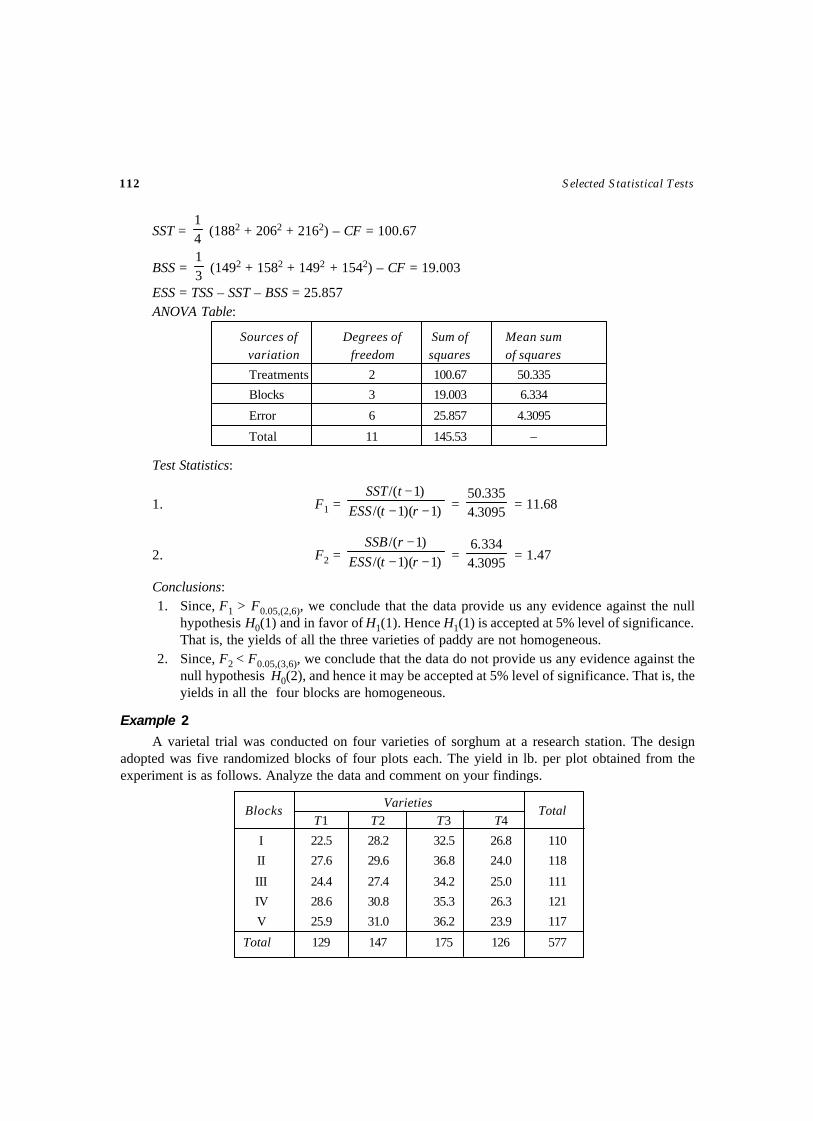
112 Selected Statistical Tests
SST = 41
(1882 + 2062 + 2162) – CF = 100.67
BSS = 31
(1492 + 1582 + 1492 + 1542) – CF = 19.003
ESS = TSS – SST – BSS = 25.857ANOVA Table:
Sources of Degrees of Sum of Mean sumvariation freedom squares of squares
Treatments 2 100.67 50.335
Blocks 3 19.003 6.334
Error 6 25.857 4.3095
Total 11 145.53 –
Test Statistics:
1. F1 = )1)(1/()1/(−−
−rtESS
tSST = 3095.4
335.50 = 11.68
2. F2 = )1)(1/()1/(−−
−rtESS
rSSB = 3095.4
334.6 = 1.47
Conclusions:1. Since, F1 > F0.05,(2,6), we conclude that the data provide us any evidence against the null
hypothesis H0(1) and in favor of H1(1). Hence H1(1) is accepted at 5% level of significance.That is, the yields of all the three varieties of paddy are not homogeneous.
2. Since, F2 < F0.05,(3,6), we conclude that the data do not provide us any evidence against thenull hypothesis H0(2), and hence it may be accepted at 5% level of significance. That is, theyields in all the four blocks are homogeneous.
Example 2
A varietal trial was conducted on four varieties of sorghum at a research station. The designadopted was five randomized blocks of four plots each. The yield in lb. per plot obtained from theexperiment is as follows. Analyze the data and comment on your findings.
VarietiesT1 T2 T3 T4
I 22.5 28.2 32.5 26.8 110
II 27.6 29.6 36.8 24.0 118
III 24.4 27.4 34.2 25.0 111
IV 28.6 30.8 35.3 26.3 121
V 25.9 31.0 36.2 23.9 117
Total 129 147 175 126 577
Blocks Total
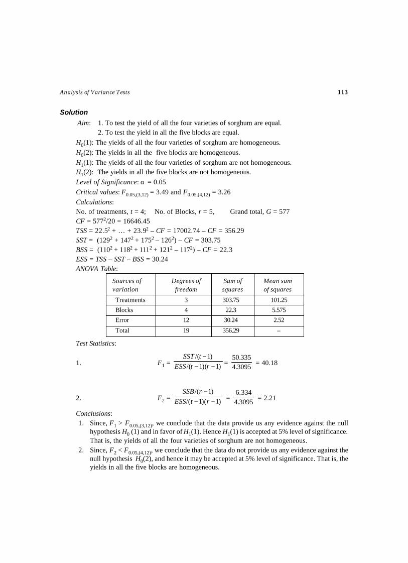
Analysis of Variance Tests 113
Solution
Aim: 1. To test the yield of all the four varieties of sorghum are equal.2. To test the yield in all the five blocks are equal.
H0(1): The yields of all the four varieties of sorghum are homogeneous.H0(2): The yields in all the five blocks are homogeneous.H1(1): The yields of all the four varieties of sorghum are not homogeneous.H1(2): The yields in all the five blocks are not homogeneous.Level of Significance: α = 0.05Critical values: F0.05,(3,12) = 3.49 and F0.05,(4,12) = 3.26Calculations:No. of treatments, t = 4; No. of Blocks, r = 5, Grand total, G = 577CF = 5772/20 = 16646.45TSS = 22.52 + … + 23.92 – CF = 17002.74 – CF = 356.29SST = (1292 + 1472 + 1752 – 1262) – CF = 303.75BSS = (1102 + 1182 + 1112 + 1212 – 1172) – CF = 22.3ESS = TSS – SST – BSS = 30.24ANOVA Table:
Sources of Degrees of Sum of Mean sumvariation freedom squares of squares
Treatments 3 303.75 101.25
Blocks 4 22.3 5.575
Error 12 30.24 2.52
Total 19 356.29 –
Test Statistics:
1. F1 = )1)(1/()1/(−−
−rtESS
tSST= 3095.4
335.50 = 40.18
2. F2 = )1)(1/()1/(−−
−rtESS
rSSB = 3095.4
334.6 = 2.21
Conclusions:1. Since, F1 > F0.05,(3,12), we conclude that the data provide us any evidence against the null
hypothesis H0 (1) and in favor of H1(1). Hence H1(1) is accepted at 5% level of significance.That is, the yields of all the four varieties of sorghum are not homogeneous.
2. Since, F2 < F0.05,(4,12), we conclude that the data do not provide us any evidence against thenull hypothesis H0(2), and hence it may be accepted at 5% level of significance. That is, theyields in all the five blocks are homogeneous.
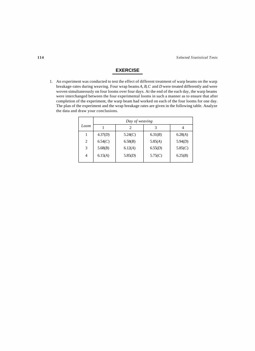
114 Selected Statistical Tests
EXERCISE
1. An experiment was conducted to test the effect of different treatment of warp beams on the warpbreakage-rates during weaving. Four wrap beams A, B, C and D were treated differently and werewoven simultaneously on four looms over four days. At the end of the each day, the warp beamswere interchanged between the four experimental looms in such a manner as to ensure that aftercompletion of the experiment, the warp beam had worked on each of the four looms for one day.The plan of the experiment and the wrap breakage rates are given in the following table. Analyzethe data and draw your conclusions.
Day of weaving
1 2 3 4
1 4.37(D) 5.24(C) 6.31(B) 6.28(A)
2 6.54(C) 6.58(B) 5.85(A) 5.94(D)
3 5.68(B) 6.12(A) 6.55(D) 5.85(C)
4 6.15(A) 5.85(D) 5.75(C) 6.25(B)
Loom
TEST FOR RANDOMIZED BLOCK DESIGN(More than one observation per cell)
TEST – 29
Aim
To test the significance of the t treatment effects and the significance of the r block effects andthe interaction between treatments and blocks based on the observations from n experimental units.
Source
Let yijk, (i = 1, 2,…, t ; j = 1, 2,…, r ; k = 1, 2,…, m) be the kth observation in the ith treatmentand in the jth block. Let n = t × r × m.
Linear Model
The linear model is yijk = µ + τi + βj + γij + εij
where µ is the overall mean effect, τi is the effect due to the ith treatment, βj is the effect due tothe jth block, γij is the interaction effect between ith treatment with jth block and εij is the error effectdue to chance causes.
Assumptions
(i) The population from which, the observations drawn is Normal distribution.(ii) The observations are independent.
(iii) The various effects are additive in nature.(iv) εij are identically independently distributed as Normal distribution with mean zero and variance
2εσ .
(v) ∑=
τt
ii
1= ∑
=
βr
jj
1= 0
(vi) ∑=
γt
iij
1= 0 for all j.
(vii) ∑=
γr
jij
1= 0 for all i.
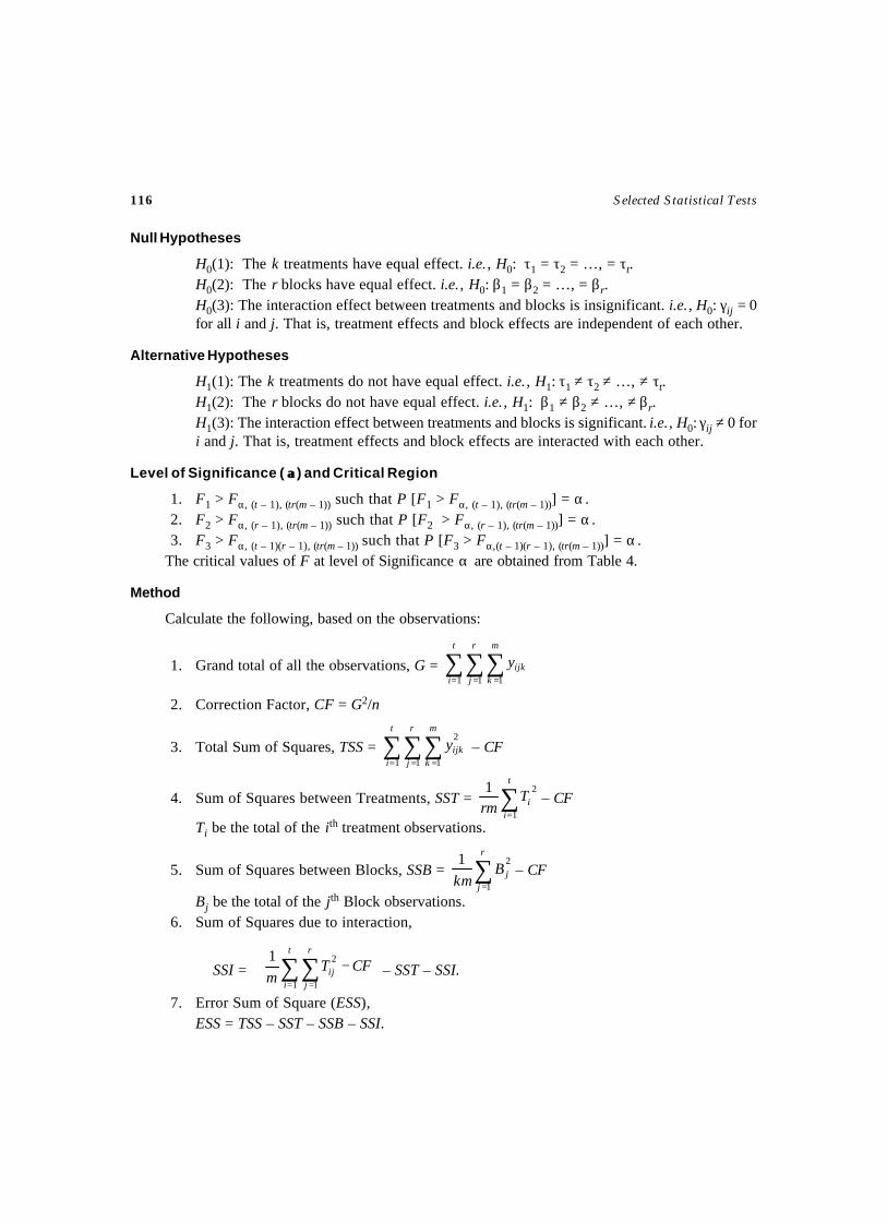
116 Selected Statistical Tests
Null Hypotheses
H0(1): The k treatments have equal effect. i.e., H0: τ1 = τ2 = …, = τt.H0(2): The r blocks have equal effect. i.e., H0: β1 = β2 = …, = βr.H0(3): The interaction effect between treatments and blocks is insignificant. i.e., H0: γij = 0for all i and j. That is, treatment effects and block effects are independent of each other.
Alternative Hypotheses
H1(1): The k treatments do not have equal effect. i.e., H1: τ1 ≠ τ2 ≠ …, ≠ τt.H1(2): The r blocks do not have equal effect. i.e., H1: β1 ≠ β2 ≠ …, ≠ βr.H1(3): The interaction effect between treatments and blocks is significant. i.e., H0: γij ≠ 0 fori and j. That is, treatment effects and block effects are interacted with each other.
Level of Significance ( αα) and Critical Region
1. F1 > Fα, (t – 1), (tr(m – 1)) such that P [F1 > Fα, (t – 1), (tr(m – 1))] = α .2. F2 > Fα, (r – 1), (tr(m – 1)) such that P [F2 > Fα, (r – 1), (tr(m – 1))] = α .3. F3 > Fα, (t – 1)(r – 1), (tr(m – 1)) such that P [F3 > Fα,(t – 1)(r – 1), (tr(m – 1))] = α .
The critical values of F at level of Significance α are obtained from Table 4.
Method
Calculate the following, based on the observations:
1. Grand total of all the observations, G = ∑∑∑= = =
t
i
r
j
m
kijky
1 1 1
2. Correction Factor, CF = G2/n
3. Total Sum of Squares, TSS = ∑∑∑= = =
t
i
r
j
m
kijky
1 1 1
2 – CF
4. Sum of Squares between Treatments, SST = ∑=
t
iiT
rm 1
21– CF
Ti be the total of the ith treatment observations.
5. Sum of Squares between Blocks, SSB = ∑=
r
jjB
km 1
21– CF
Bj be the total of the jth Block observations.6. Sum of Squares due to interaction,
SSI =
−∑∑
= =
CFTm
t
i
r
jij
1 1
21– SST – SSI.
7. Error Sum of Square (ESS),ESS = TSS – SST – SSB – SSI.
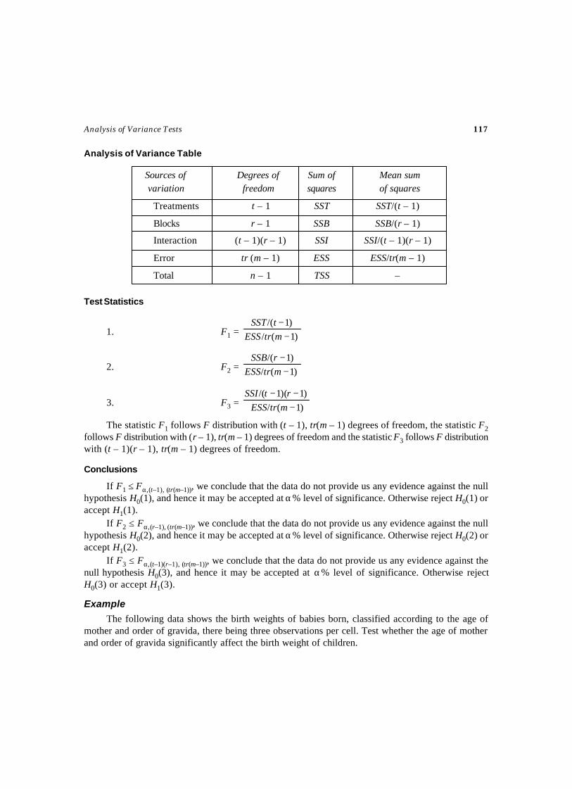
Analysis of Variance Tests 117
Analysis of Variance Table
Sources of Degrees of Sum of Mean sumvariation freedom squares of squares
Treatments t – 1 SST SST/(t – 1)
Blocks r – 1 SSB SSB/(r – 1)
Interaction (t – 1)(r – 1) SSI SSI/(t – 1)(r – 1)
Error tr (m – 1) ESS ESS/tr(m – 1)
Total n – 1 TSS –
Test Statistics
1. F1 = )1(/)1/(
−−
mtrESStSST
2. F2 = )1(/)1/(
−−
mtrESSrSSB
3. F3 = )1(/)1)(1/(
−−−
mtrESSrtSSI
The statistic F1 follows F distribution with (t – 1), tr(m – 1) degrees of freedom, the statistic F2follows F distribution with (r – 1), tr(m – 1) degrees of freedom and the statistic F3 follows F distributionwith (t – 1)(r – 1), tr(m – 1) degrees of freedom.
Conclusions
If F1 ≤ Fα,(t–1), (tr(m–1)), we conclude that the data do not provide us any evidence against the nullhypothesis H0(1), and hence it may be accepted at α% level of significance. Otherwise reject H0(1) oraccept H1(1).
If F2 ≤ Fα,(r–1), (tr(m–1)), we conclude that the data do not provide us any evidence against the nullhypothesis H0(2), and hence it may be accepted at α% level of significance. Otherwise reject H0(2) oraccept H1(2).
If F3 ≤ Fα,(t–1)(r–1), (tr(m–1)), we conclude that the data do not provide us any evidence against thenull hypothesis H0(3), and hence it may be accepted at α% level of significance. Otherwise rejectH0(3) or accept H1(3).
Example
The following data shows the birth weights of babies born, classified according to the age ofmother and order of gravida, there being three observations per cell. Test whether the age of motherand order of gravida significantly affect the birth weight of children.
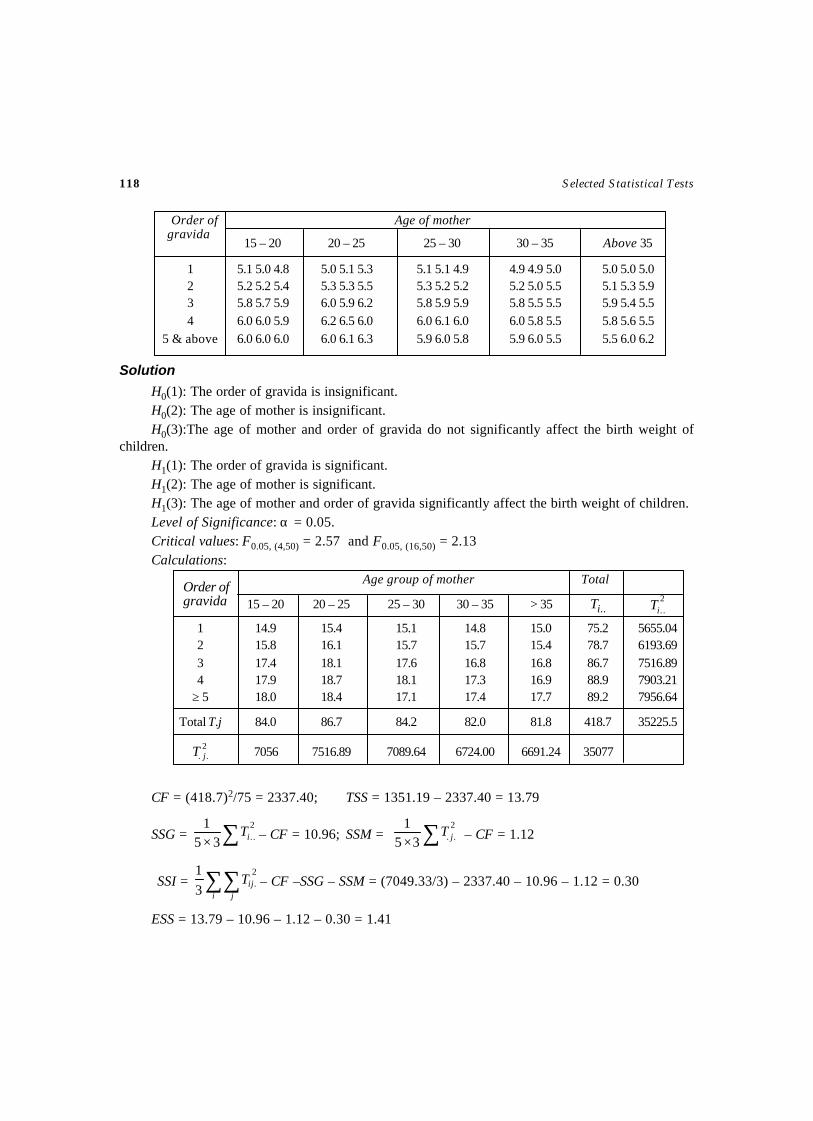
118 Selected Statistical Tests
Order of Age of mother
15 – 20 20 – 25 25 – 30 30 – 35 Above 35
1 5.1 5.0 4.8 5.0 5.1 5.3 5.1 5.1 4.9 4.9 4.9 5.0 5.0 5.0 5.02 5.2 5.2 5.4 5.3 5.3 5.5 5.3 5.2 5.2 5.2 5.0 5.5 5.1 5.3 5.93 5.8 5.7 5.9 6.0 5.9 6.2 5.8 5.9 5.9 5.8 5.5 5.5 5.9 5.4 5.54 6.0 6.0 5.9 6.2 6.5 6.0 6.0 6.1 6.0 6.0 5.8 5.5 5.8 5.6 5.5
5 & above 6.0 6.0 6.0 6.0 6.1 6.3 5.9 6.0 5.8 5.9 6.0 5.5 5.5 6.0 6.2
Solution
H0(1): The order of gravida is insignificant.H0(2): The age of mother is insignificant.H0(3):The age of mother and order of gravida do not significantly affect the birth weight of
children.H1(1): The order of gravida is significant.H1(2): The age of mother is significant.H1(3): The age of mother and order of gravida significantly affect the birth weight of children.Level of Significance: α = 0.05.Critical values: F0.05, (4,50) = 2.57 and F0.05, (16,50) = 2.13Calculations:
Age group of mother Total
15 – 20 20 – 25 25 – 30 30 – 35 > 35 ..iT 2..iT
1 14.9 15.4 15.1 14.8 15.0 75.2 5655.042 15.8 16.1 15.7 15.7 15.4 78.7 6193.693 17.4 18.1 17.6 16.8 16.8 86.7 7516.894 17.9 18.7 18.1 17.3 16.9 88.9 7903.21
≥ 5 18.0 18.4 17.1 17.4 17.7 89.2 7956.64
Total T.j 84.0 86.7 84.2 82.0 81.8 418.7 35225.5
2.. jT 7056 7516.89 7089.64 6724.00 6691.24 35077
CF = (418.7)2/75 = 2337.40; TSS = 1351.19 – 2337.40 = 13.79
SSG = ∑×2..35
1iT – CF = 10.96; SSM = ∑×
2..35
1jT – CF = 1.12
SSI = ∑∑i j
ijT2.3
1– CF –SSG – SSM = (7049.33/3) – 2337.40 – 10.96 – 1.12 = 0.30
ESS = 13.79 – 10.96 – 1.12 – 0.30 = 1.41
Order ofgravida
gravida
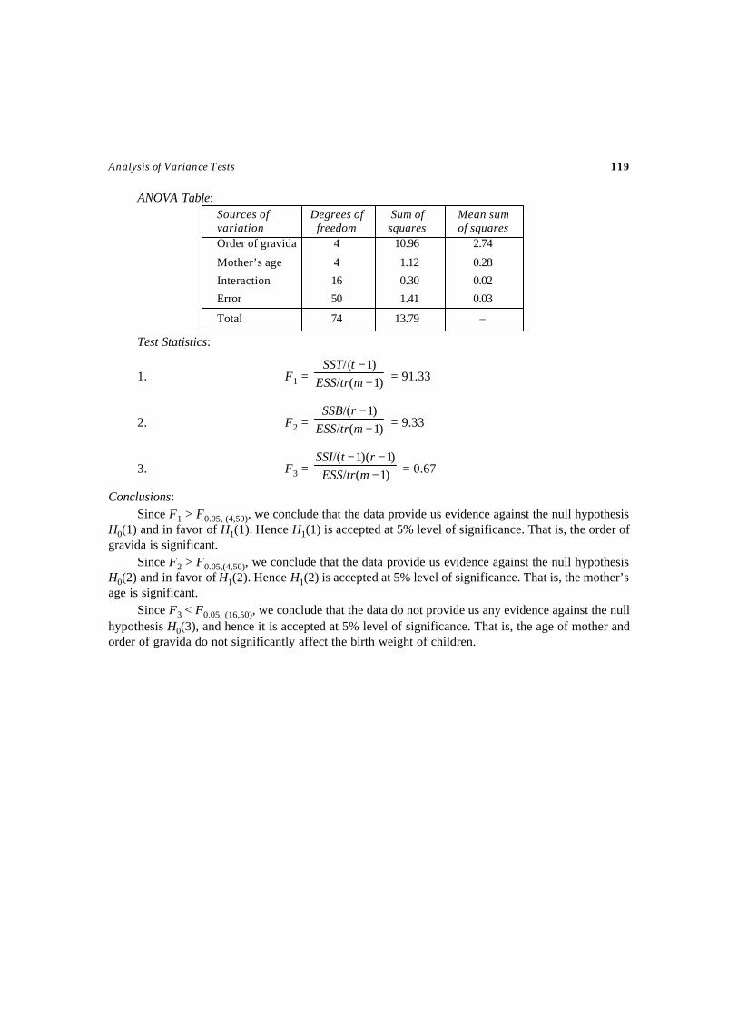
Analysis of Variance Tests 119
ANOVA Table:Sources of Degrees of Sum of Mean sumvariation freedom squares of squaresOrder of gravida 4 10.96 2.74
Mother’s age 4 1.12 0.28
Interaction 16 0.30 0.02
Error 50 1.41 0.03
Total 74 13.79 –
Test Statistics:
1. F1 = )1(/)1(/
−−
mtrESStSST
= 91.33
2. F2 = )1(/)1(/
−−
mtrESSrSSB
= 9.33
3. F3 = )1(/)1)(1(/
−−−
mtrESSrtSSI
= 0.67
Conclusions:Since F1 > F0.05, (4,50), we conclude that the data provide us evidence against the null hypothesis
H0(1) and in favor of H1(1). Hence H1(1) is accepted at 5% level of significance. That is, the order ofgravida is significant.
Since F2 > F0.05,(4,50), we conclude that the data provide us evidence against the null hypothesisH0(2) and in favor of H1(2). Hence H1(2) is accepted at 5% level of significance. That is, the mother’sage is significant.
Since F3 < F0.05, (16,50), we conclude that the data do not provide us any evidence against the nullhypothesis H0(3), and hence it is accepted at 5% level of significance. That is, the age of mother andorder of gravida do not significantly affect the birth weight of children.

ANOCOVA TEST FOR RANDOMIZED BLOCKDESIGN
TEST – 30
Aim
To test the significance of the treatment effects and the significance of the regression coefficientof Y on X, based on the observations from n experimental units under randomized block design.
Source
Let (Yij, Xij) (i = 1, 2, …, t ; j = 1, 2, …, r) be the observations made from an experiment consistsof t treatments each with r blocks (replications) on two variables Y and X. The observations on auxiliaryor concomitant variable, X apart from the main variable Y under study is available for each of theexperimental units. When Y and X are associated, a part of the variation of Y is due to variation in valuesof X. After eliminating, the effects of blocks and treatments one can then estimate a relationship,between Y and X and use that relationship to predict the value of Y for a given value of X. This test isused for assessing the significance of relationship between X and Y. If there is, a significant associationbetween X and Y one may calculate the adjusted treatment sum of squares and perform the test for thehomogeneity of treatment effects. Let n = t × r. The observed data is arranged as follows:
Block
1 2 … t
Y X Y X … Y X Y X
1 Y11 X11 Y21 X21 … Yt1 Xt1 BY1 BX1
2 Y12 X12 Y22 X22 … Yt2 Xt2 BY1 BX1
… … … … … … … … … …
… … … … … … … … … …
… … … … … … … … … …
r Y1r X1r Y2r X2r … Ytr Xtr BY1 BX1
Treatment
TY1 TX1 TY2 TX2 … TYt TXt GY GX
totalsBlocks Treatments
totals
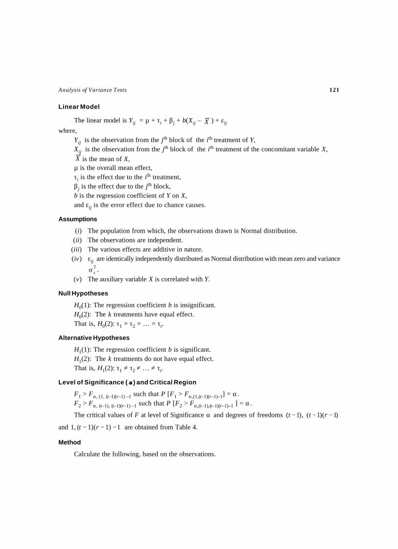
Analysis of Variance Tests 121
Linear Model
The linear model is Yij = µ + τi + βj + b(Xij – X ) + εij
where,Yij is the observation from the jth block of the ith treatment of Y,Xij is the observation from the jth block of the ith treatment of the concomitant variable X,X is the mean of X,µ is the overall mean effect,τi is the effect due to the ith treatment,βj is the effect due to the jth block,b is the regression coefficient of Y on X,and εij is the error effect due to chance causes.
Assumptions
(i) The population from which, the observations drawn is Normal distribution.(ii) The observations are independent.
(iii) The various effects are additive in nature.(iv) εij are identically independently distributed as Normal distribution with mean zero and variance
2εσ .
(v) The auxiliary variable X is correlated with Y.
Null Hypotheses
H0(1): The regression coefficient b is insignificant.H0(2): The k treatments have equal effect.That is, H0(2): τ1 = τ2 = … = τt.
Alternative Hypotheses
H1(1): The regression coefficient b is significant.H1(2): The k treatments do not have equal effect.That is, H1(2): τ1 ≠ τ2 ≠ … ≠ τt.
Level of Significance ( αα) and Critical Region
F1 > Fα, (1, (t–1)(r–1) –1 such that P [F1 > Fα,(1,(t–1)(r–1)–1] = α .F2 > Fα, (t–1), (t–1)(r–1) –1 such that P [F2 > Fα,(t–1),(t–1)(r–1)–1 ] = α .
The critical values of F at level of Significance α and degrees of freedoms )1)(1(),1( −−− rtt
and 1111 −−− ))((, rt are obtained from Table 4.
Method
Calculate the following, based on the observations.
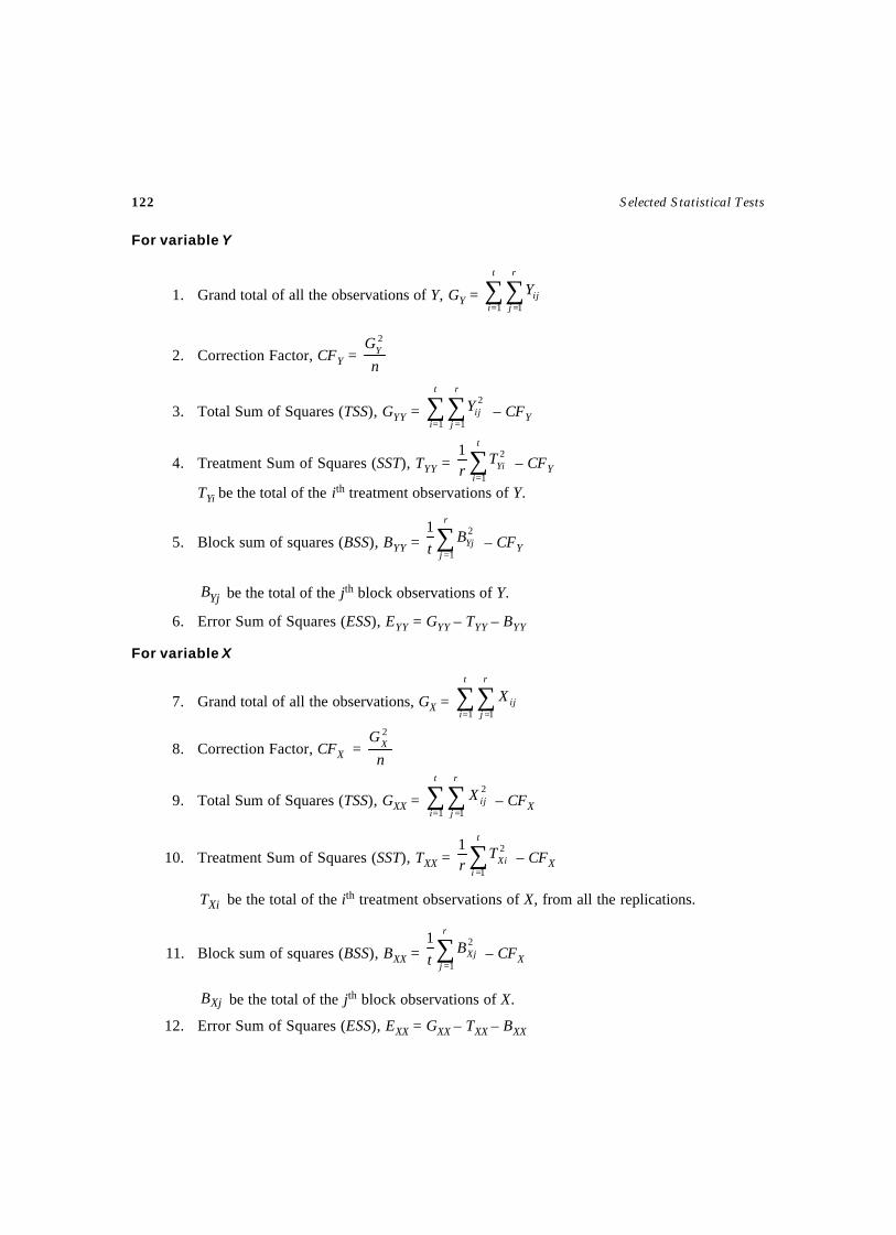
122 Selected Statistical Tests
For variable Y
1. Grand total of all the observations of Y, GY = ∑∑= =
t
i
r
jijY
1 1
2. Correction Factor, CFY = n
GY2
3. Total Sum of Squares (TSS), GYY = ∑∑= =
t
i
r
jijY
1 1
2 – CFY
4. Treatment Sum of Squares (SST), TYY = ∑=
t
iYiT
r 1
21 – CFY
TYi be the total of the ith treatment observations of Y.
5. Block sum of squares (BSS), BYY = ∑=
r
jYjB
t 1
21 – CFY
YjB be the total of the jth block observations of Y.
6. Error Sum of Squares (ESS), EYY = GYY – TYY – BYY
For variable X
7. Grand total of all the observations, GX = ∑∑= =
t
i
r
jijX
1 1
8. Correction Factor, CFX = n
GX2
9. Total Sum of Squares (TSS), GXX = ∑∑= =
t
i
r
jijX
1 1
2 – CFX
10. Treatment Sum of Squares (SST), TXX = ∑=
t
iXiT
r 1
21 – CFX
XiT be the total of the ith treatment observations of X, from all the replications.
11. Block sum of squares (BSS), BXX = ∑=
r
jXjB
t 1
21 – CFX
XjB be the total of the jth block observations of X.
12. Error Sum of Squares (ESS), EXX = GXX – TXX – BXX
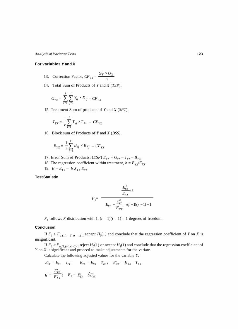
Analysis of Variance Tests 123
For variables Y and X
13. Correction Factor, CFYX = n
GG XY ×
14. Total Sum of Products of Y and X (TSP),
GYX = ∑∑= =
×t
i
r
jijij XY
1 1– CFYX
15. Treatment Sum of products of Y and X (SPT),
TYX = ∑=
×t
iXiYi TT
r 1
1 – CFYX
16. Block sum of Products of Y and X (BSS),
BYX = ∑=
×r
jXjYj BB
t 1
1 – CFYX
17. Error Sum of Products, (ESP) EYX = GYX – TYX – BYX
18. The regression coefficient within treatment, b = EYX/EXX
19. E = EYY – b XYX EYX
Test Statistic
F1=
−−−
−
1)1)(1/(
1/
2
2
rtEEE
EE
XX
YXYY
XX
YX
F1 follows F distribution with 1, (r – 1)(t – 1) – 1 degrees of freedom.
Conclusion
If F1 ≤ Fα,(1(t – 1) (r – 1)–1 accept H0(1) and conclude that the regression coefficient of Y on X isinsignificant.
If F1 > Fα,(1,(t–1)(r–1)-1 reject H0(1) or accept H1(1) and conclude that the regression coefficient ofY on X is significant and proceed to make adjustments for the variate.
Calculate the following adjusted values for the variable Y:
YYYYYY TEE +=′ ; YXYXYX TEE +=′ ; XXXXXX TEE +=′
b~ =
XX
YX
EE
′′
; E1 = YXYY EbE ′−′~
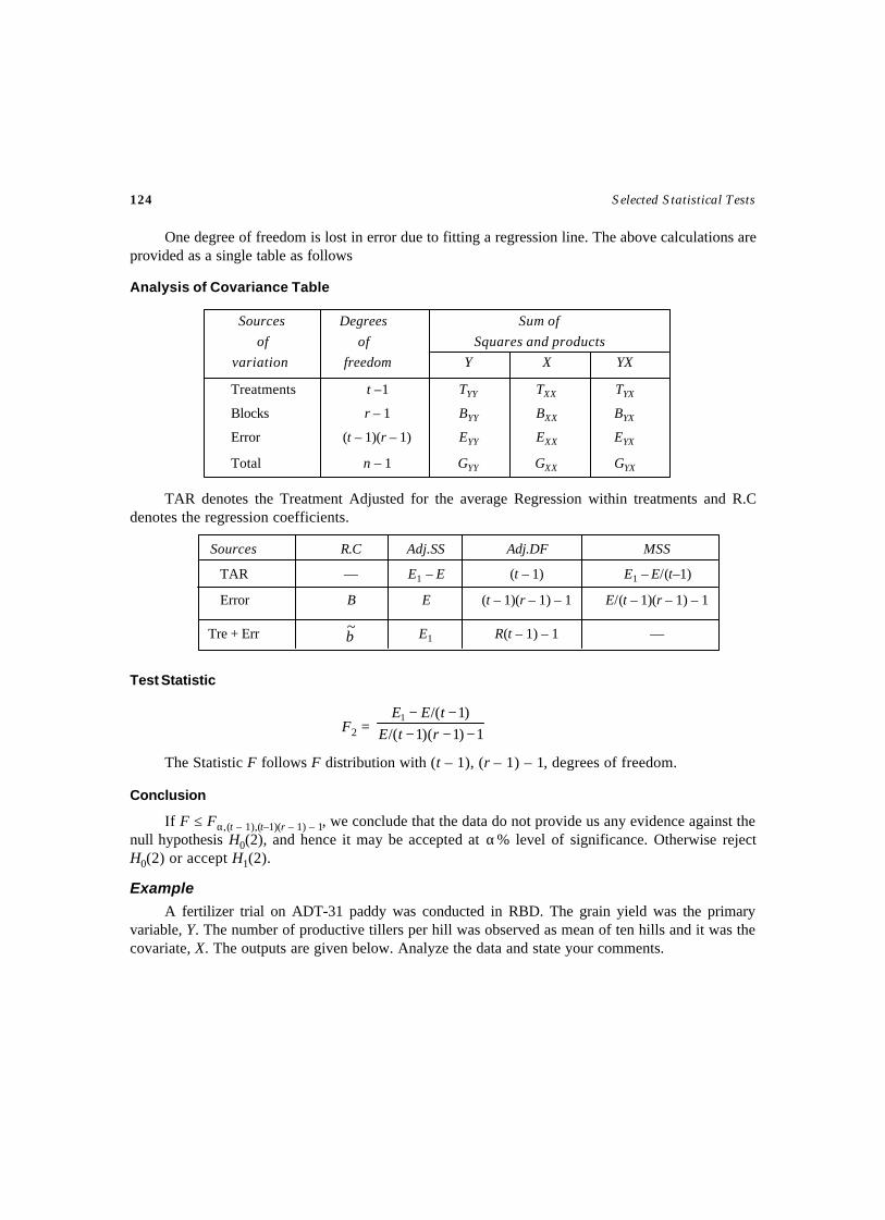
124 Selected Statistical Tests
One degree of freedom is lost in error due to fitting a regression line. The above calculations areprovided as a single table as follows
Analysis of Covariance Table
Sources Degrees Sum of
of of Squares and products
variation freedom Y X YX
Treatments t –1 TYY TXX TYX
Blocks r – 1 BYY BXX BYX
Error (t – 1)(r – 1) EYY EXX EYX
Total n – 1 GYY GXX GYX
TAR denotes the Treatment Adjusted for the average Regression within treatments and R.Cdenotes the regression coefficients.
Sources R.C Adj.SS Adj.DF MSS
TAR — E1 – E (t – 1) E1 – E/(t–1)
Error B E (t – 1)(r – 1) – 1 E/(t – 1)(r – 1) – 1
Tre + Err b~ E1 R(t – 1) – 1 —
Test Statistic
F2 = 1)1)(1(/)1(/1
−−−−−
rtEtEE
The Statistic F follows F distribution with (t – 1), (r – 1) – 1, degrees of freedom.
Conclusion
If F ≤ Fα,(t – 1),(t–1)(r – 1) – 1, we conclude that the data do not provide us any evidence against thenull hypothesis H0(2), and hence it may be accepted at α% level of significance. Otherwise rejectH0(2) or accept H1(2).
Example
A fertilizer trial on ADT-31 paddy was conducted in RBD. The grain yield was the primaryvariable, Y. The number of productive tillers per hill was observed as mean of ten hills and it was thecovariate, X. The outputs are given below. Analyze the data and state your comments.
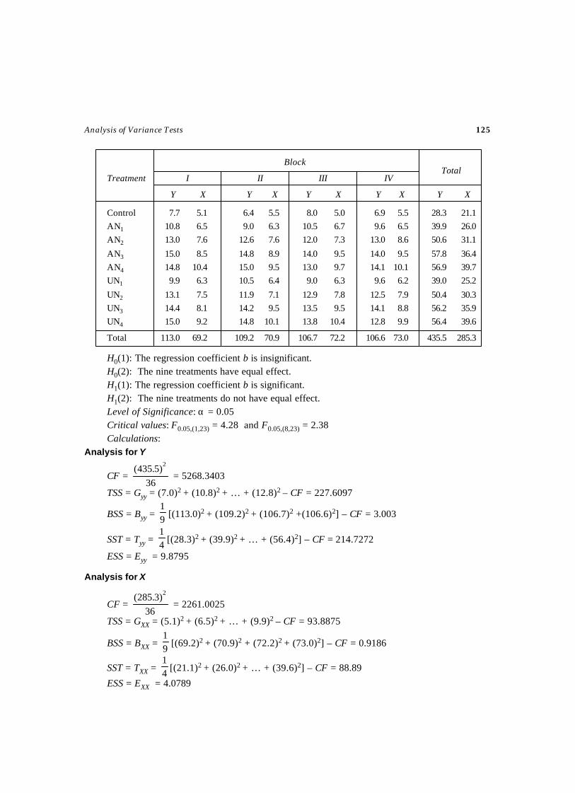
Analysis of Variance Tests 125
Block
Treatment I II III IV
Y X Y X Y X Y X Y X
Control 7.7 5.1 6.4 5.5 8.0 5.0 6.9 5.5 28.3 21.1
AN1 10.8 6.5 9.0 6.3 10.5 6.7 9.6 6.5 39.9 26.0
AN2 13.0 7.6 12.6 7.6 12.0 7.3 13.0 8.6 50.6 31.1
AN3 15.0 8.5 14.8 8.9 14.0 9.5 14.0 9.5 57.8 36.4
AN4 14.8 10.4 15.0 9.5 13.0 9.7 14.1 10.1 56.9 39.7
UN1 9.9 6.3 10.5 6.4 9.0 6.3 9.6 6.2 39.0 25.2
UN2 13.1 7.5 11.9 7.1 12.9 7.8 12.5 7.9 50.4 30.3
UN3 14.4 8.1 14.2 9.5 13.5 9.5 14.1 8.8 56.2 35.9
UN4 15.0 9.2 14.8 10.1 13.8 10.4 12.8 9.9 56.4 39.6
Total 113.0 69.2 109.2 70.9 106.7 72.2 106.6 73.0 435.5 285.3
H0(1): The regression coefficient b is insignificant.H0(2): The nine treatments have equal effect.H1(1): The regression coefficient b is significant.H1(2): The nine treatments do not have equal effect.Level of Significance: α = 0.05Critical values: F0.05,(1,23) = 4.28 and F0.05,(8,23) = 2.38Calculations:
Analysis for Y
CF = 36
)5.435( 2
= 5268.3403
TSS = Gyy = (7.0)2 + (10.8)2 + … + (12.8)2 – CF = 227.6097
BSS = Byy = 91
[(113.0)2 + (109.2)2 + (106.7)2 +(106.6)2] – CF = 3.003
SST = Tyy = 41
[(28.3)2 + (39.9)2 + … + (56.4)2] – CF = 214.7272
ESS = Eyy = 9.8795
Analysis for X
CF = 36
)3.285( 2
= 2261.0025
TSS = GXX = (5.1)2 + (6.5)2 + … + (9.9)2 – CF = 93.8875
BSS = BXX = 91
[(69.2)2 + (70.9)2 + (72.2)2 + (73.0)2] – CF = 0.9186
SST = TXX = 41
[(21.1)2 + (26.0)2 + … + (39.6)2] – CF = 88.89
ESS = EXX = 4.0789
Total
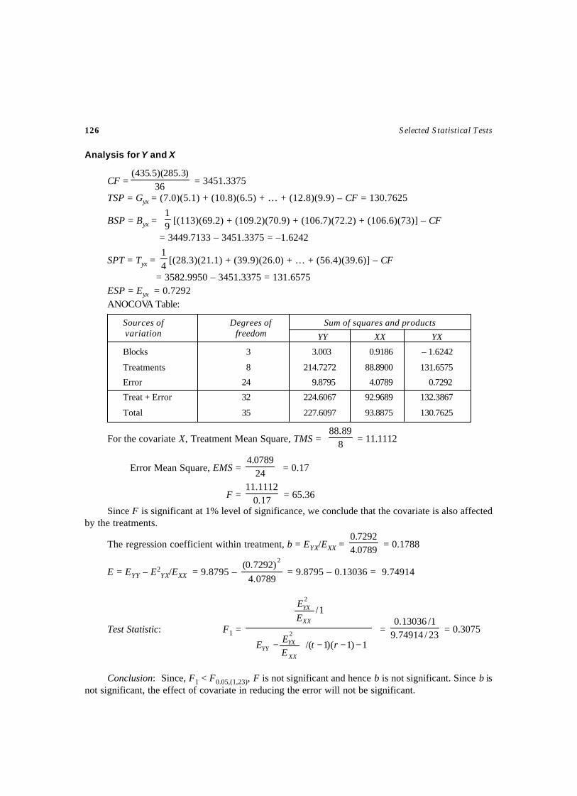
126 Selected Statistical Tests
Analysis for Y and X
CF = 36)3.285)(5.435(
= 3451.3375
TSP = Gyx = (7.0)(5.1) + (10.8)(6.5) + … + (12.8)(9.9) – CF = 130.7625
BSP = Byx = 91
[(113)(69.2) + (109.2)(70.9) + (106.7)(72.2) + (106.6)(73)] – CF
= 3449.7133 – 3451.3375 = –1.6242
SPT = Tyx = 41
[(28.3)(21.1) + (39.9)(26.0) + … + (56.4)(39.6)] – CF
= 3582.9950 – 3451.3375 = 131.6575ESP = Eyx = 0.7292ANOCOVA Table:
Sources of Degrees of Sum of squares and products
YY XX YX
Blocks 3 3.003 0.9186 – 1.6242
Treatments 8 214.7272 88.8900 131.6575
Error 24 9.8795 4.0789 0.7292
Treat + Error 32 224.6067 92.9689 132.3867
Total 35 227.6097 93.8875 130.7625
For the covariate X, Treatment Mean Square, TMS = 889.88
= 11.1112
Error Mean Square, EMS = 240789.4
= 0.17
F = 17.01112.11
= 65.36
Since F is significant at 1% level of significance, we conclude that the covariate is also affectedby the treatments.
The regression coefficient within treatment, b = EYX/EXX = 0789.47292.0
= 0.1788
E = EYY – E2YX/EXX = 9.8795 –
0789.4)7292.0( 2
= 9.8795 – 0.13036 = 9.74914
Test Statistic: F1 =
−−−
−
1)1)(1/(
1/
2
2
rtEEE
EE
XX
YXYY
XX
YX
= 23/74914.91/13036.0
= 0.3075
Conclusion: Since, F1 < F0.05,(1,23), F is not significant and hence b is not significant. Since b isnot significant, the effect of covariate in reducing the error will not be significant.
variation freedom
TEST FOR LATIN SQUARE DESIGN
TEST – 31
Aim
To test the significance of the m treatment effects, m row effects and m column effects based onthe observations from m square (m2) experimental units.
Source
Let yijk, (i, j, k = 1, 2,…, m) be the observations of m treatments, each applied with (equal numberof replications) m times in m2 experimental units. In this design, the entire experimental material isdivided into m2 experimental units arranged in a square so that each row and each column contains munits. The m treatments are allocated at random to these rows and columns in such a way that everytreatment occurs once and only once in each row and in each column.
This design is very much advantageous in the sense that, the treatment effect, the two orthogonaleffects such as row and column effects can be studied simultaneously in m square experimental units.
Linear Model
The linear model is yijk = µ + τi + βj + νk + εijk; (i, j, k = 1, 2,…, m)where yijk is the observation of the ith treatment obtained from the jth row and kth column, µ is theoverall mean effect, τi is the effect due to the ith treatment, βj is the effect due to the jth row, νk is theeffect due to the kth column and εijk is the error effect due to chance causes.
Assumptions
(i) The population from which, the observations drawn is Normal distribution.(ii) The observations are independent.
(iii) The various effects are additive in nature.(iv) εijk are identically independently distributed as Normal distribution with mean zero and
variance 2εσ .
Null Hypotheses
H0(1): The m treatments have equal effect. i.e., H0(1): τ1 = τ2 = …, = τm.
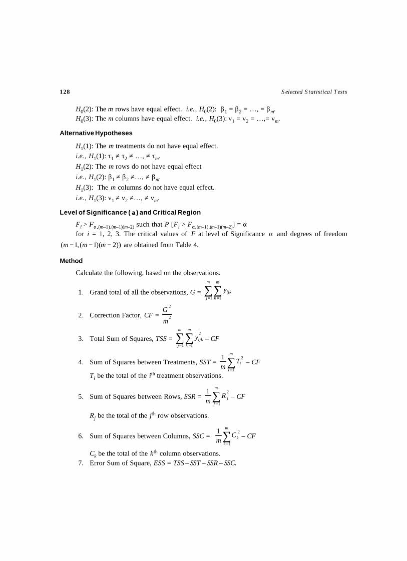
128 Selected Statistical Tests
H0(2): The m rows have equal effect. i.e., H0(2): β1 = β2 = …, = βm.H0(3): The m columns have equal effect. i.e., H0(3): ν1 = ν2 = …,= νm.
Alternative Hypotheses
H1(1): The m treatments do not have equal effect.i.e., H1(1): τ1 ≠ τ2 ≠ …, ≠ τm.
H1(2): The m rows do not have equal effect
i.e., H1(2): β1 ≠ β2 ≠…, ≠ βm.
H1(3): The m columns do not have equal effect.
i.e., H1(3): ν1 ≠ ν2 ≠…, ≠ νm.
Level of Significance ( αα) and Critical Region
Fi > Fα,(m–1),(m–1)(m–2) such that P [Fi > Fα,(m–1),(m–1)(m–2)] = αfor i = 1, 2, 3. The critical values of F at level of Significance α and degrees of freedom
))2)(1(,1( −−− mmm are obtained from Table 4.
Method
Calculate the following, based on the observations.
1. Grand total of all the observations, G = ∑∑= =
m
j
m
kijky
1 1
2. Correction Factor, CF = 2
2
m
G
3. Total Sum of Squares, TSS = ∑∑= =
m
j
m
kijky
1 1
2– CF
4. Sum of Squares between Treatments, SST = ∑=
m
iiT
m 1
21– CF
Ti be the total of the ith treatment observations.
5. Sum of Squares between Rows, SSR = ∑=
m
jjR
m 1
21– CF
Rj be the total of the jth row observations.
6. Sum of Squares between Columns, SSC = ∑=
m
kkC
m 1
21– CF
Ck be the total of the kth column observations.7. Error Sum of Square, ESS = TSS – SST – SSR – SSC.
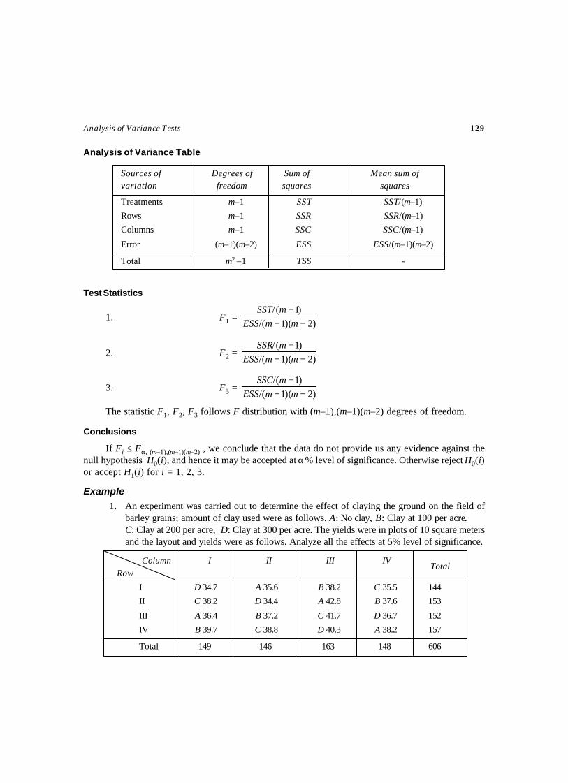
Analysis of Variance Tests 129
Analysis of Variance Table
Sources of Degrees of Sum of Mean sum ofvariation freedom squares squares
Treatments m–1 SST SST/(m–1)
Rows m–1 SSR SSR/(m–1)
Columns m–1 SSC SSC/(m–1)
Error (m–1)(m–2) ESS ESS/(m–1)(m–2)
Total m2 –1 TSS -
Test Statistics
1. F1 =)2)(1(/
)1(/−−
−mmESS
mSST
2. F2 =)2)(1(/
)1(/−−
−mmESS
mSSR
3. F3 =)2)(1(/
)1(/−−
−mmESS
mSSC
The statistic F1, F2, F3 follows F distribution with (m–1),(m–1)(m–2) degrees of freedom.
Conclusions
If Fi ≤ Fα, (m–1),(m–1)(m–2) , we conclude that the data do not provide us any evidence against thenull hypothesis H0(i), and hence it may be accepted at α% level of significance. Otherwise reject H0(i)or accept H1(i) for i = 1, 2, 3.
Example
1. An experiment was carried out to determine the effect of claying the ground on the field ofbarley grains; amount of clay used were as follows. A: No clay, B: Clay at 100 per acre.C: Clay at 200 per acre, D: Clay at 300 per acre. The yields were in plots of 10 square metersand the layout and yields were as follows. Analyze all the effects at 5% level of significance.
Column I II III IVRow
I D 34.7 A 35.6 B 38.2 C 35.5 144
II C 38.2 D 34.4 A 42.8 B 37.6 153
III A 36.4 B 37.2 C 41.7 D 36.7 152
IV B 39.7 C 38.8 D 40.3 A 38.2 157
Total 149 146 163 148 606
Total
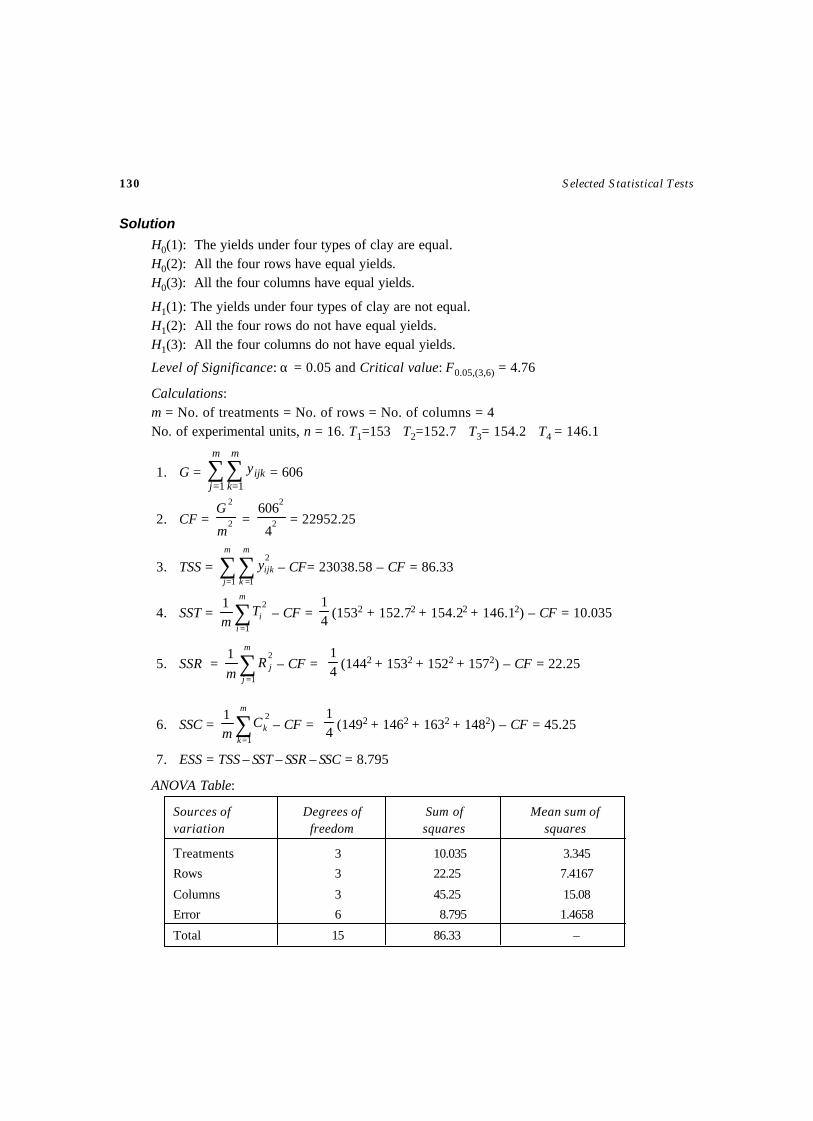
130 Selected Statistical Tests
Solution
H0(1): The yields under four types of clay are equal.H0(2): All the four rows have equal yields.H0(3): All the four columns have equal yields.
H1(1): The yields under four types of clay are not equal.H1(2): All the four rows do not have equal yields.H1(3): All the four columns do not have equal yields.
Level of Significance: α = 0.05 and Critical value: F0.05,(3,6) = 4.76
Calculations:m = No. of treatments = No. of rows = No. of columns = 4No. of experimental units, n = 16. T1=153 T2=152.7 T3= 154.2 T4 = 146.1
1. G = ∑∑= =
m
j
m
kijky
1 1= 606
2. CF = 2
2
m
G = 2
2
4
606= 22952.25
3. TSS = ∑∑= =
m
j
m
kijky
1 1
2– CF= 23038.58 – CF = 86.33
4. SST = ∑=
m
iiT
m 1
21– CF = 4
1(1532 + 152.72 + 154.22 + 146.12) – CF = 10.035
5. SSR = ∑=
m
jjR
m 1
21– CF = 4
1(1442 + 1532 + 1522 + 1572) – CF = 22.25
6. SSC = ∑=
m
kkC
m 1
21– CF = 4
1(1492 + 1462 + 1632 + 1482) – CF = 45.25
7. ESS = TSS – SST – SSR – SSC = 8.795
ANOVA Table:
Sources of Degrees of Sum of Mean sum ofvariation freedom squares squares
Treatments 3 10.035 3.345
Rows 3 22.25 7.4167
Columns 3 45.25 15.08
Error 6 8.795 1.4658
Total 15 86.33 –
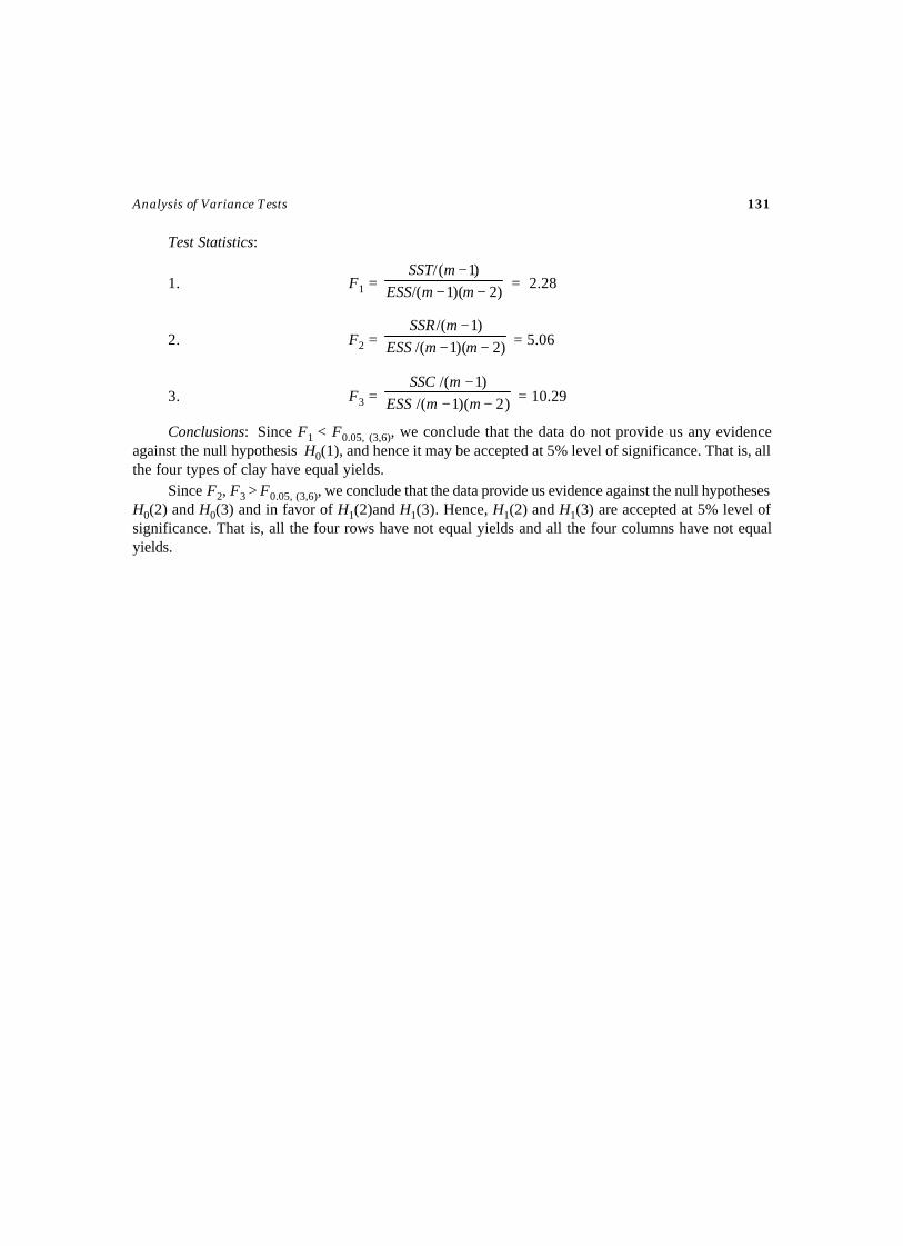
Analysis of Variance Tests 131
Test Statistics:
1. F1 = )2)(1(/)1(/−−
−mmESS
mSST = 2.28
2. F2 = )2)(1/()1/(−−
−mmESS
mSSR = 5.06
3. F3 = )2)(1/()1/(−−
−mmESS
mSSC = 10.29
Conclusions: Since F1 < F0.05, (3,6), we conclude that the data do not provide us any evidenceagainst the null hypothesis H0(1), and hence it may be accepted at 5% level of significance. That is, allthe four types of clay have equal yields.
Since F2, F3 > F0.05, (3,6), we conclude that the data provide us evidence against the null hypothesesH0(2) and H0(3) and in favor of H1(2)and H1(3). Hence, H1(2) and H1(3) are accepted at 5% level ofsignificance. That is, all the four rows have not equal yields and all the four columns have not equalyields.

TEST FOR 22 FACTORIAL DESIGN
TEST – 32
Aim
To test the significance of the main effects and interaction effect based on experiment consists oftwo factors each with two levels.
Source
In this design, let there be two treatments (Factors) say, A and B are called simple treatmentswhose effects can be tested with two levels, say 0 (absent) and 1 (present). That is, we study theindividual effects of A and B as well as their combined effect, called as interaction. This 22 factorialdesign consists of 4 treatment combinations namely A0B0, A1B0, A0B1, A1B1 are denoted by ‘1’ (bothat 0 level indicate no application of factor), main effect A, main effect B and interaction AB. It can betested in r blocks (replications), so that it requires r × 22 = 4r = n experimental units. [1], [a], [b] and[ab] are called treatment totals, denote, respectively the observations of the treatments ‘1’, ‘a’, ‘b’ and‘ab’ from all the r blocks.
Null Hypotheses
H0(1): All the r blocks have equal effect.H0(2): The main effect A is insignificant.H0(3): The main effect B is insignificant.H0(4): The interaction AB is insignificant.
Alternative Hypotheses
H1(1): All the r blocks do not have equal effect.H1(2): The main effect A is significant.H1(3): The main effect B is significant.H1(4): The interaction AB is significant.
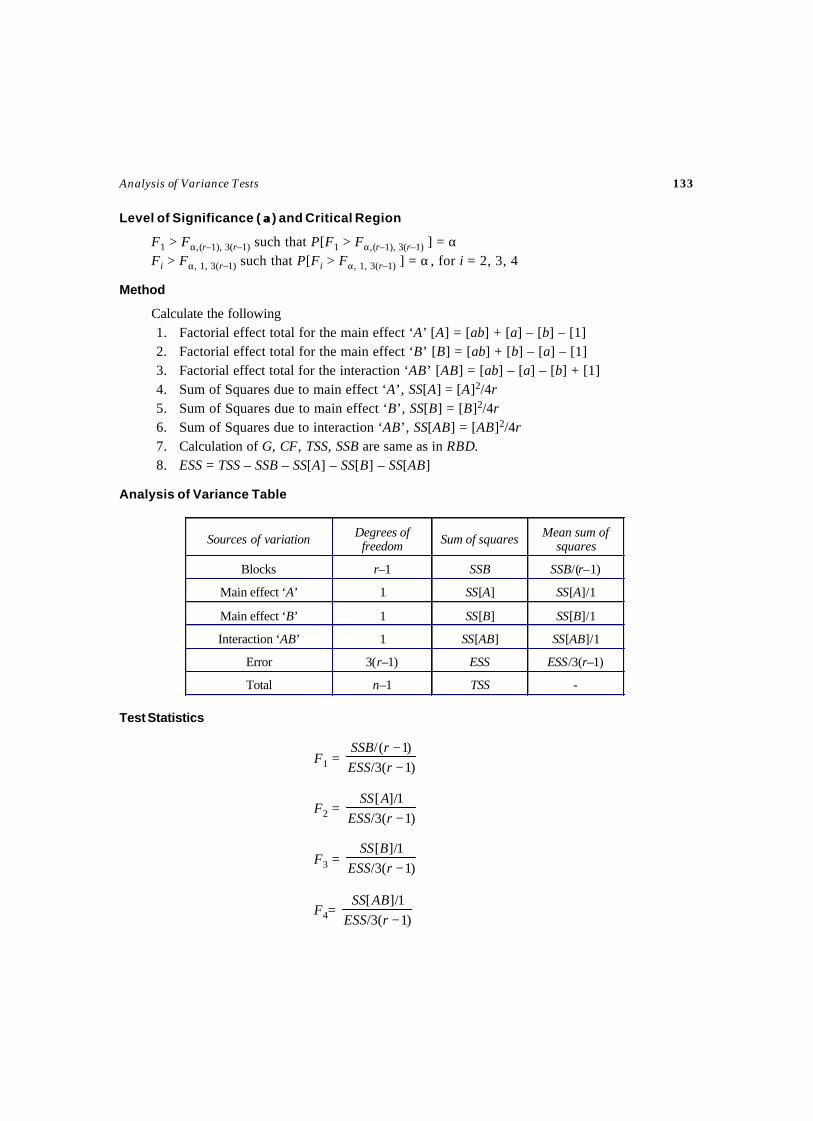
Analysis of Variance Tests 133
Level of Significance ( αα) and Critical Region
F1 > Fα,(r–1), 3(r–1) such that P[F1 > Fα,(r–1), 3(r–1) ] = αFi > Fα, 1, 3(r–1) such that P[Fi > Fα, 1, 3(r–1) ] = α , for i = 2, 3, 4
Method
Calculate the following1. Factorial effect total for the main effect ‘A’ [A] = [ab] + [a] – [b] – [1]2. Factorial effect total for the main effect ‘B’ [B] = [ab] + [b] – [a] – [1]3. Factorial effect total for the interaction ‘AB’ [AB] = [ab] – [a] – [b] + [1]4. Sum of Squares due to main effect ‘A’, SS[A] = [A]2/4r5. Sum of Squares due to main effect ‘B’, SS[B] = [B]2/4r6. Sum of Squares due to interaction ‘AB’, SS[AB] = [AB]2/4r7. Calculation of G, CF, TSS, SSB are same as in RBD.8. ESS = TSS – SSB – SS[A] – SS[B] – SS[AB]
Analysis of Variance Table
Test Statistics
F1 =)1(3/
)1(/−−
rESSrSSB
F2 = )1(3/
1/][−rESS
ASS
F3 =)1(3/
1/][−rESS
BSS
F4= )1(3/
1/][−rESS
ABSS
Sources of variation Degrees of freedom Sum of squares Mean sum of
squares
Blocks r–1 SSB SSB/(r–1)
Main effect ‘A’ 1 SS[A] SS[A]/1
Main effect ‘B’ 1 SS[B] SS[B]/1
Interaction ‘AB’ 1 SS[AB] SS[AB]/1
Error 3(r–1) ESS ESS/3(r–1)
Total n–1 TSS -
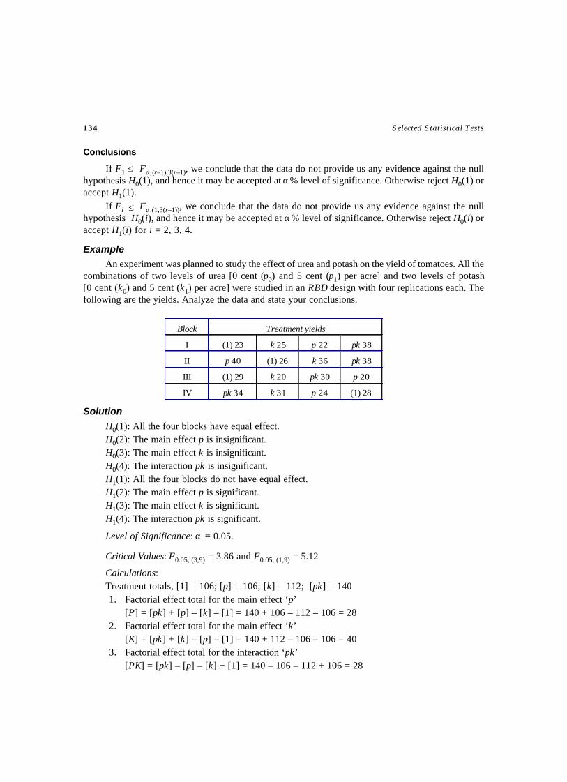
134 Selected Statistical Tests
Conclusions
If F1 ≤ Fα,(r–1),3(r–1), we conclude that the data do not provide us any evidence against the nullhypothesis H0(1), and hence it may be accepted at α% level of significance. Otherwise reject H0(1) oraccept H1(1).
If Fi ≤ Fα,(1,3(r–1)), we conclude that the data do not provide us any evidence against the nullhypothesis H0(i), and hence it may be accepted at α% level of significance. Otherwise reject H0(i) oraccept H1(i) for i = 2, 3, 4.
Example
An experiment was planned to study the effect of urea and potash on the yield of tomatoes. All thecombinations of two levels of urea [0 cent (p0) and 5 cent (p1) per acre] and two levels of potash[0 cent (k0) and 5 cent (k1) per acre] were studied in an RBD design with four replications each. Thefollowing are the yields. Analyze the data and state your conclusions.
Solution
H0(1): All the four blocks have equal effect.H0(2): The main effect p is insignificant.H0(3): The main effect k is insignificant.H0(4): The interaction pk is insignificant.H1(1): All the four blocks do not have equal effect.H1(2): The main effect p is significant.H1(3): The main effect k is significant.H1(4): The interaction pk is significant.
Level of Significance: α = 0.05.
Critical Values: F0.05, (3,9) = 3.86 and F0.05, (1,9) = 5.12
Calculations:Treatment totals, [1] = 106; [p] = 106; [k] = 112; [pk] = 1401. Factorial effect total for the main effect ‘p’
[P] = [pk] + [p] – [k] – [1] = 140 + 106 – 112 – 106 = 282. Factorial effect total for the main effect ‘k’
[K] = [pk] + [k] – [p] – [1] = 140 + 112 – 106 – 106 = 403. Factorial effect total for the interaction ‘pk’
[PK] = [pk] – [p] – [k] + [1] = 140 – 106 – 112 + 106 = 28
Block Treatment yields
I (1) 23 k 25 p 22 pk 38
II p 40 (1) 26 k 36 pk 38
III (1) 29 k 20 pk 30 p 20
IV pk 34 k 31 p 24 (1) 28
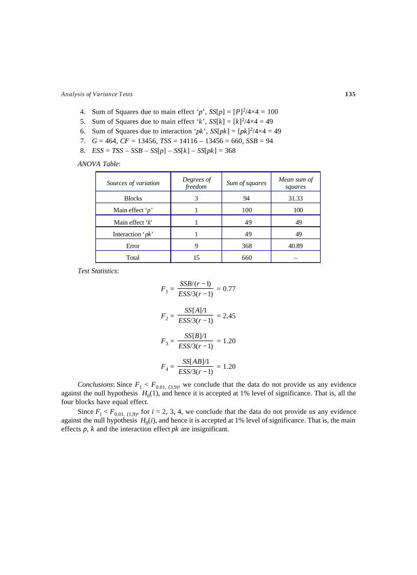
Analysis of Variance Tests 135
4. Sum of Squares due to main effect ‘p’, SS[p] = [P]2/4×4 = 1005. Sum of Squares due to main effect ‘k’, SS[k] = [k]2/4×4 = 496. Sum of Squares due to interaction ‘pk’, SS[pk] = [pk]2/4×4 = 497. G = 464, CF = 13456, TSS = 14116 – 13456 = 660, SSB = 948. ESS = TSS – SSB – SS[p] – SS[k] – SS[pk] = 368
ANOVA Table:
Test Statistics:
F1 =)1(3/
)1(/−−
rESSrSSB
= 0.77
F2 =)1(3/
1/][−rESS
ASS = 2.45
F3 =)1(3/
1/][−rESS
BSS = 1.20
F4 =)1(3/
1/][−rESS
ABSS = 1.20
Conclusions: Since F1 < F0.01, (3,9), we conclude that the data do not provide us any evidenceagainst the null hypothesis H0(1), and hence it is accepted at 1% level of significance. That is, all thefour blocks have equal effect.
Since Fi < F0.01, (1,9), for i = 2, 3, 4, we conclude that the data do not provide us any evidenceagainst the null hypothesis H0(i), and hence it is accepted at 1% level of significance. That is, the maineffects p, k and the interaction effect pk are insignificant.
Sources of variation Degrees of freedom Sum of squares Mean sum of
squares
Blocks 3 94 31.33
Main effect ‘p’ 1 100 100
Main effect ‘k’ 1 49 49
Interaction ‘pk’ 1 49 49
Error 9 368 40.89
Total 15 660 –

TEST FOR 23 FACTORIAL DESIGN
TEST – 33
Aim
To test the significance of the main effects and interaction effect based on experiment consists ofthree factors each with two levels.
Source
In this design, let there be three treatments (Factors) say, A, B and C are called simple treatmentswhose effects can be tested with two levels, say 0 (absent) and 1 (present). That is, we study theindividual effects of A, B and C as well as their combined effects, called as interactions. This 23
factorial design consists of 8 treatment combinations namely A0B0C0, A1B0C0, A0B1C0, A0B0C1, A1B1C0,A1B0C1, A0B1C1 and A1B1C1 are denoted by ‘1’ (all at 0 levels indicate no application of factor), maineffects A, B, C and interactions AB, AC, ABC. It can be tested in r blocks (replications), so that itrequires r × 23 = 8r = n experimental units. [1], [a], [b], [c], [ab], [ac], [bc] and [abc] are calledtreatment totals, denote, respectively the observations of the treatments ‘1’, ‘a’, ‘b’, ‘c’, ‘ab’, ‘ac’,‘bc’ and ‘abc’ from all the r blocks.
Null Hypotheses
H0(1): All the r blocks have equal effect.H0(2): The main effect A is insignificant.H0(3): The main effect B is insignificant.H0(4): The main effect C is insignificant.H0(5): The interaction AB insignificant.H0(6): The interaction AC insignificant.H0(7): The interaction BC insignificant.H0(8): The interaction ABC insignificant.
Alternative Hypotheses
H1(1): All the r blocks do not have equal effect.H1(2): The main effect A is significant.
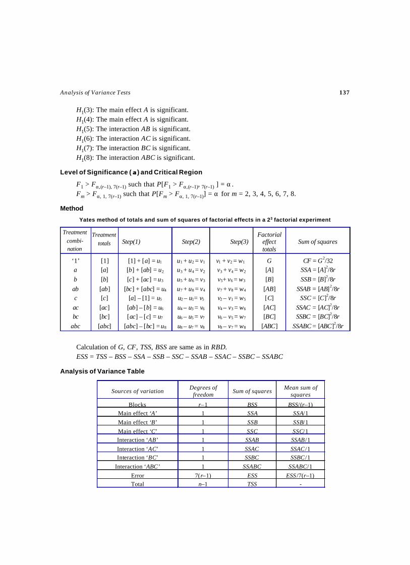
Analysis of Variance Tests 137
H1(3): The main effect A is significant.H1(4): The main effect A is significant.H1(5): The interaction AB is significant.H1(6): The interaction AC is significant.H1(7): The interaction BC is significant.H1(8): The interaction ABC is significant.
Level of Significance ( αα) and Critical Region
F1 > Fα,(r–1), 7(r–1) such that P[F1 > Fα,(r–1), 7(r–1) ] = α.Fm > Fα, 1, 7(r–1) such that P[Fm > Fα, 1, 7(r–1)] = α for m = 2, 3, 4, 5, 6, 7, 8.
Method
Yates method of totals and sum of squares of factorial effects in a 23 factorial experiment
Calculation of G, CF, TSS, BSS are same as in RBD.ESS = TSS – BSS – SSA – SSB – SSC – SSAB – SSAC – SSBC – SSABC
Analysis of Variance Table
Sources of variation Degrees of
freedom Sum of squares
Mean sum of squares
Blocks r–1 BSS BSS/(r–1) Main effect ‘A’ 1 SSA SSA/1
Main effect ‘B’ 1 SSB SSB/1
Main effect ‘C’ 1 SSC SSC/1 Interaction ‘AB’ 1 SSAB SSAB /1
Interaction ‘AC’ 1 SSAC SSAC /1 Interaction ‘BC’ 1 SSBC SSBC /1
Interaction ‘ABC’ 1 SSABC SSABC/1
Error 7(r–1) ESS ESS /7(r–1) Total n–1 TSS -
Step(1) Step(2) Step(3) Factorial
effect totals
Sum of squares
‘1’ a
b
ab c
ac bc
abc
[1] [a]
[b]
[ab] [c]
[ac] [bc]
[abc]
[1] + [a] = u1 [b] + [ab] = u2
[c] + [ac] = u3
[bc] + [abc] = u4 [a] – [1] = u5
[ab] – [b] = u6 [ac] – [c] = u7
[abc] – [bc] = u8
u1 + u2 = v1 u3 + u4 = v2
u5 + u6 = v3
u7 + u8 = v4 u2 – u1= v5
u4 – u3 = v6 u6 – u5 = v7
u8 – u7 = v8
v1 + v2 = w1 v3 + v4 = w2
v5+ v6 = w3
v7 + v8 = w4 v2 – v1 = w5
v4 – v3 = w6 v6 – v5 = w7
v8 – v7 = w8
G [A]
[B]
[AB] [C]
[AC] [BC]
[ABC]
CF = G2/32 SSA = [A]2/8r
SSB = [B]2/8r
SSAB = [AB]2/8r SSC = [C]2/8r
SSAC = [AC]2/8r SSBC = [BC]2/8r
SSABC = [ABC]2/8r
Treatmentcombi-nation
Treatmenttotals
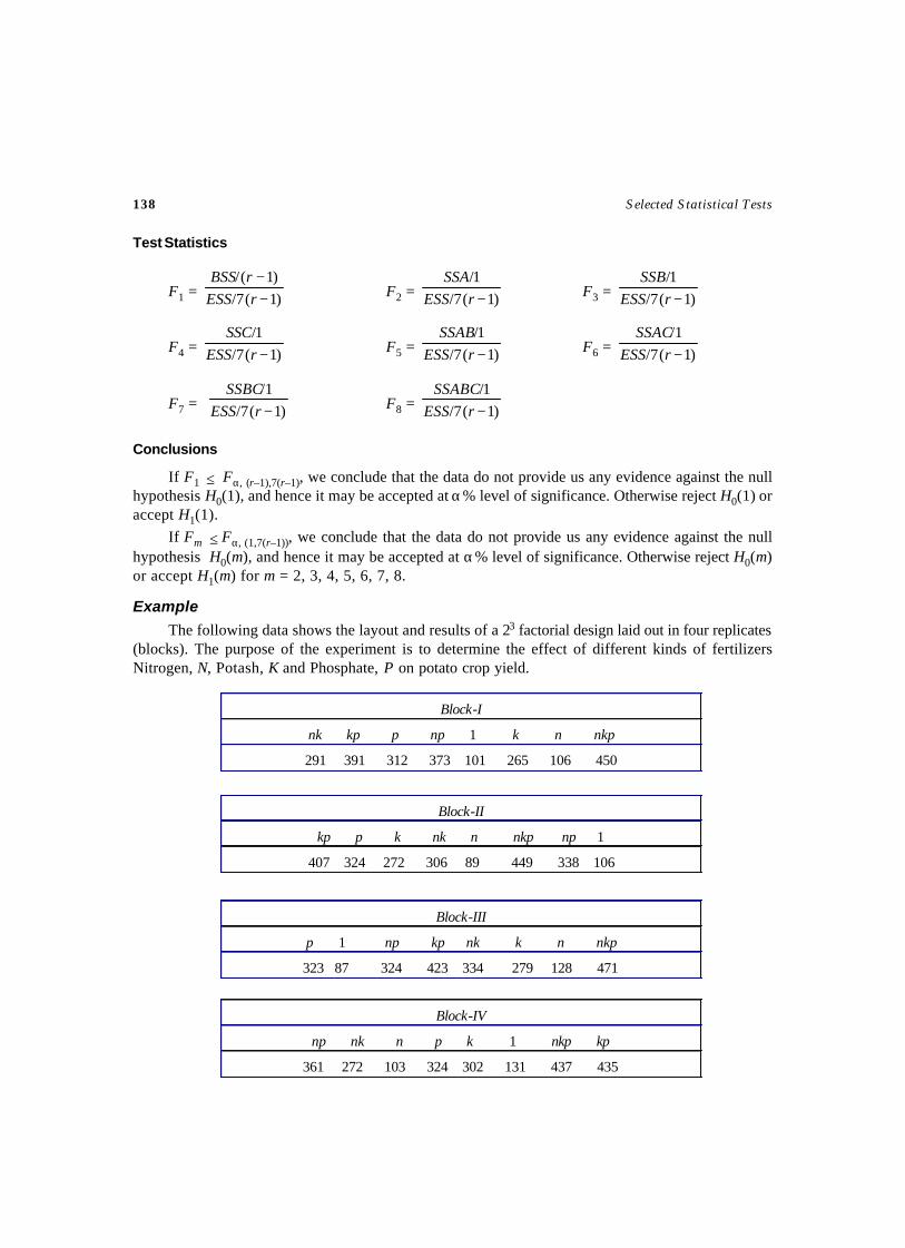
138 Selected Statistical Tests
Test Statistics
F1 = )1(7/)1(/
−−
rESSrBSS
F2 = )1(7/1/−rESS
SSAF3 = )1(7/
1/−rESS
SSB
F4 = )1(7/1/−rESS
SSCF5 = )1(7/
1/−rESS
SSABF6 = )1(7/
1/−rESS
SSAC
F7 = )1(7/1/−rESS
SSBCF8 = )1(7/
1/−rESS
SSABC
Conclusions
If F1 ≤ Fα, (r–1),7(r–1), we conclude that the data do not provide us any evidence against the nullhypothesis H0(1), and hence it may be accepted at α% level of significance. Otherwise reject H0(1) oraccept H1(1).
If Fm ≤ Fα, (1,7(r–1)), we conclude that the data do not provide us any evidence against the nullhypothesis H0(m), and hence it may be accepted at α% level of significance. Otherwise reject H0(m)or accept H1(m) for m = 2, 3, 4, 5, 6, 7, 8.
Example
The following data shows the layout and results of a 23 factorial design laid out in four replicates(blocks). The purpose of the experiment is to determine the effect of different kinds of fertilizersNitrogen, N, Potash, K and Phosphate, P on potato crop yield.
Block-I
nk kp p np 1 k n nkp
291 391 312 373 101 265 106 450
Block-II
kp p k nk n nkp np 1
407 324 272 306 89 449 338 106
Block-III
p 1 np kp nk k n nkp
323 87 324 423 334 279 128 471
Block-IV
np nk n p k 1 nkp kp
361 272 103 324 302 131 437 435
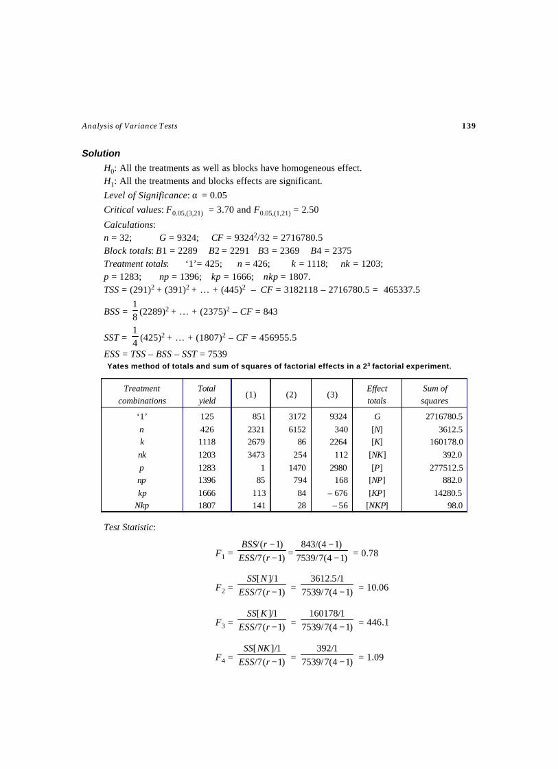
Analysis of Variance Tests 139
Solution
H0: All the treatments as well as blocks have homogeneous effect.H1: All the treatments and blocks effects are significant.
Level of Significance: α = 0.05
Critical values: F0.05,(3,21) = 3.70 and F0.05,(1,21) = 2.50
Calculations:n = 32; G = 9324; CF = 93242/32 = 2716780.5Block totals: B1 = 2289 B2 = 2291 B3 = 2369 B4 = 2375Treatment totals: ‘1’= 425; n = 426; k = 1118; nk = 1203;p = 1283; np = 1396; kp = 1666; nkp = 1807.TSS = (291)2 + (391)2
+ … + (445)2 – CF = 3182118 – 2716780.5 = 465337.5
BSS = 81
(2289)2 + … + (2375)2 – CF = 843
SST = 41
(425)2 + … + (1807)2 – CF = 456955.5
ESS = TSS – BSS – SST = 7539Yates method of totals and sum of squares of factorial effects in a 23 factorial experiment.
Test Statistic:
F1 = )1(7/)1(/
−−
rESSrBSS
= )14(7/7539)14(/843
−−
= 0.78
F2 = )1(7/1/][−rESS
NSS = )14(7/7539
1/5.3612− = 10.06
F3 = )1(7/1/][−rESS
KSS = )14(7/7539
1/160178− = 446.1
F4 = )1(7/1/][
−rESSNKSS
= )14(7/75391/392
− = 1.09
Treatment combinations
Total yield
(1) (2) (3) Effect totals
Sum of squares
‘1’
n k
nk
p np
kp Nkp
125
426 1118
1203
1283 1396
1666 1807
851
2321 2679
3473
1 85
113 141
3172
6152 86
254
1470 794
84 28
9324
340 2264
112
2980 168
– 676 – 56
G
[N] [K]
[NK]
[P] [NP]
[KP] [NKP]
2716780.5
3612.5 160178.0
392.0
277512.5 882.0
14280.5 98.0
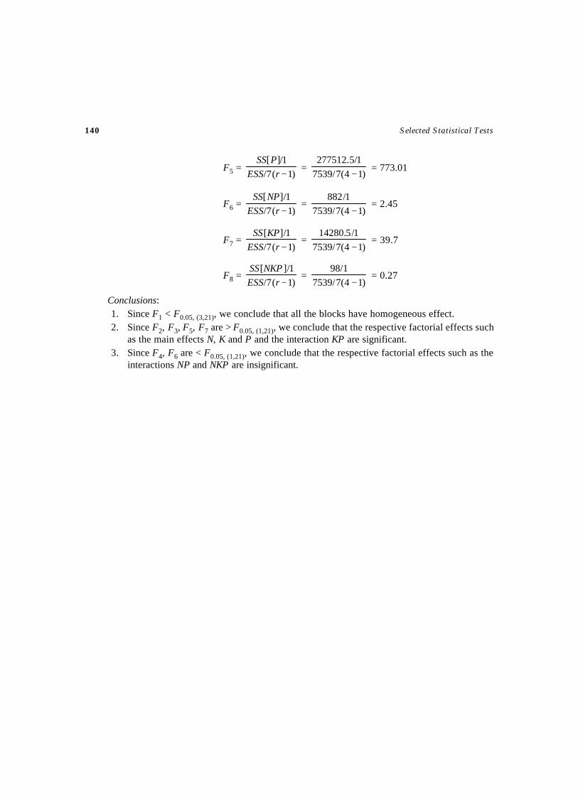
140 Selected Statistical Tests
F5 =)1(7/
1/][−rESS
PSS =
)14(7/75391/5.277512
− = 773.01
F6 =)1(7/
1/][−rESS
NPSS =
)14(7/75391/882
− = 2.45
F7 =)1(7/
1/][−rESS
KPSS =
)14(7/75391/5.14280−
= 39.7
F8 =)1(7/
1/][−rESS
NKPSS =
)14(7/75391/98
− = 0.27
Conclusions:1. Since F1 < F0.05, (3,21), we conclude that all the blocks have homogeneous effect.2. Since F2, F3, F5, F7 are > F0.05, (1,21), we conclude that the respective factorial effects such
as the main effects N, K and P and the interaction KP are significant.3. Since F4, F6 are < F0.05, (1,21), we conclude that the respective factorial effects such as the
interactions NP and NKP are insignificant.
TEST FOR SPLIT PLOT DESIGN
TEST – 34
Aim
To test the significance of the effect of main plot treatments and the effect of sub plot treatments.
Source
Suppose we are interested to test two factors ‘a’ and ‘b’, factor ‘a’ being at p levels a1, a2,…, apand factor ‘b’ at q levels b1, b2, …, bq. The different types of treatments are allotted at random to theirrespective plots. Such arrangement is split-plot design. In this design, the larger plots are called mainplots and the smaller plots within the larger plots are called sub-plot treatments. The factor levelsallotted to the main plots are called main plot treatments and the factor levels allotted to the sub-plot arecalled sub-plot treatments. The factor that requires greater precision is assigned to the sub-plots. Thereplication is then divided into number of main plots equivalent to the main plot treatments. Each mainplot is divided into sub-plots depending on the number of sub-plot treatments.
Hence, there are p main plot treatments, q sub plot treatments and r blocks (replications), so thatthere are rpq = n experimental units in total. The observations are arranged in a three-way table.
Linear Model
The model for this experiment in randomized blocks isYijk = µ + bi + mj + mij + sk + δjk + εijk.(i = 1, 2, …, r; j = 1, 2, …, p; k = 1, 2,…, q)WhereYijk is the observation of the ith block, jth main plot and kth sub plot.µ is the overall mean effect.bi is the effect due to the ith block.mj is the effect due to the jth main plot treatment.mij is the main plot error or error (A).sk is the effect due to the kth sub plot treatment.δjk is the effect due to interaction between main and sub plots.and εijk is the error effect due to sub plot and interaction or error (B).
142 Selected Statistical Tests
Assumptions
1. The main plot treatments are allocated randomly to each of the blocks.2. The sub plot treatments are allocated randomly within the main plot treatments.3. bi, mij and εijk are independently normally distributed each with mean zero and variance
22 , mb σσ and 2εσ respectively..
4. .0,0,0,0 kjsmj
jkk
jkk
kj
j ⋅∀=δ⋅∀=δ== ∑∑∑∑ LL
Null Hypotheses
H0(1): The m main plot treatments have equal effect. i.e., H0(1): m1 = m2 = …, = mp.H0(2): The s sub plot treatments have equal effect. i.e., H0(2): s1 = s2 = …, = sq.H0(3): There is no interaction between main and sub plot treatments. i.e., H0(3): δjk = 0 for all j
and k.
Alternative Hypotheses
H1(1): The m main plot treatments do not have equal effect. i.e., H0(1): m1 ≠ m2 ≠ …, ≠ mp.H1(2): The s sub plot treatments do not have equal effect. i.e., H0(2): s1 ≠ s2 ≠ …, ≠ sp.H0(3): There is interaction between main and sub plot treatments. i.e., H0(3): δjk ≠ 0 for all j
and k.
Level of Significance ( αα) and Critical Region
F1 > Fα,(p–1),(r–1)(p–1) such that P [F1 > Fα,(p–1),(r–1)(p–1)] = α.F2 > Fα,(q–1),(r–1)p(q–1) such that P [F2 > Fα,(q–1),(r–1)p(q–1)] = α.F3 > Fα,(p–1)(q–1),(r–1)p(q–1) such that P [F3 > Fα,(p–1)(q–1),(r–1)p(q–1)] = α.The critical values of F at level of Significance α and for respective degrees of freedom, are
obtained from Table 4.
Method
Calculate the following, based on the observations.
Main Plot Analysis
1. Grand total of all the n observations, G = ∑∑∑= = =
r
i
p
j
q
kijky
1 1 1
2. Correction Factor, CF = n
G 2
3. Total Sum of Squares, TSS = ∑∑∑= = =
r
i
p
j
q
kijky
1 1 1
2
– CF
4. Form a two-way table (BM table) for Blocks × Main plot treatments as follows.
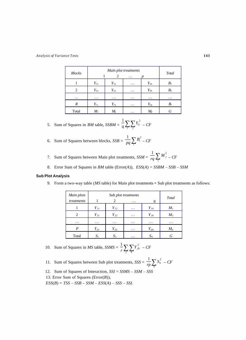
Analysis of Variance Tests 143
5. Sum of Squares in BM table, SSBM = ∑∑i j
ijYq
2.
1 – CF
6. Sum of Squares between blocks, SSB = ∑i
iBpq
21– CF
7. Sum of Squares between Main plot treatments, SSM = ∑j
jMrq
21– CF
8. Error Sum of Squares in BM table (Error(A)), ESS(A) = SSBM – SSB – SSM
Sub Plot Analysis
9. Form a two-way table (MS table) for Main plot treatments × Sub plot treatments as follows:
10. Sum of Squares in MS table, SSMS = ∑∑j k
jkYr
2.
1 – CF
11. Sum of Squares between Sub plot treatments, SSS = ∑k
kSrp
21 – CF
12. Sum of Squares of Interaction, SSI = SSMS – SSM – SSS13. Error Sum of Squares (Error(B)),ESS(B) = TSS – SSB – SSM – ESS(A) – SSS – SSI.
Blocks
Main plot treatments
1 2 … p Total
1 Y11. Y12. … Y1p. B1
2 Y21. Y22. … Y2p. B2
… … … … … …
R Yr1. Yr2. … Yrp. Br
Total M1 M2 … Mp G
Main plots
treatments
Sub plot treatments
1 2 … q Total
1 Y.11 Y.12 … Y.1q M1
2 Y.21 Y.22 … Y.2q M2
… … … … … …
P Y.p1 Y.p2 … Y.pq Mp
Total S1 S2 … Sq G
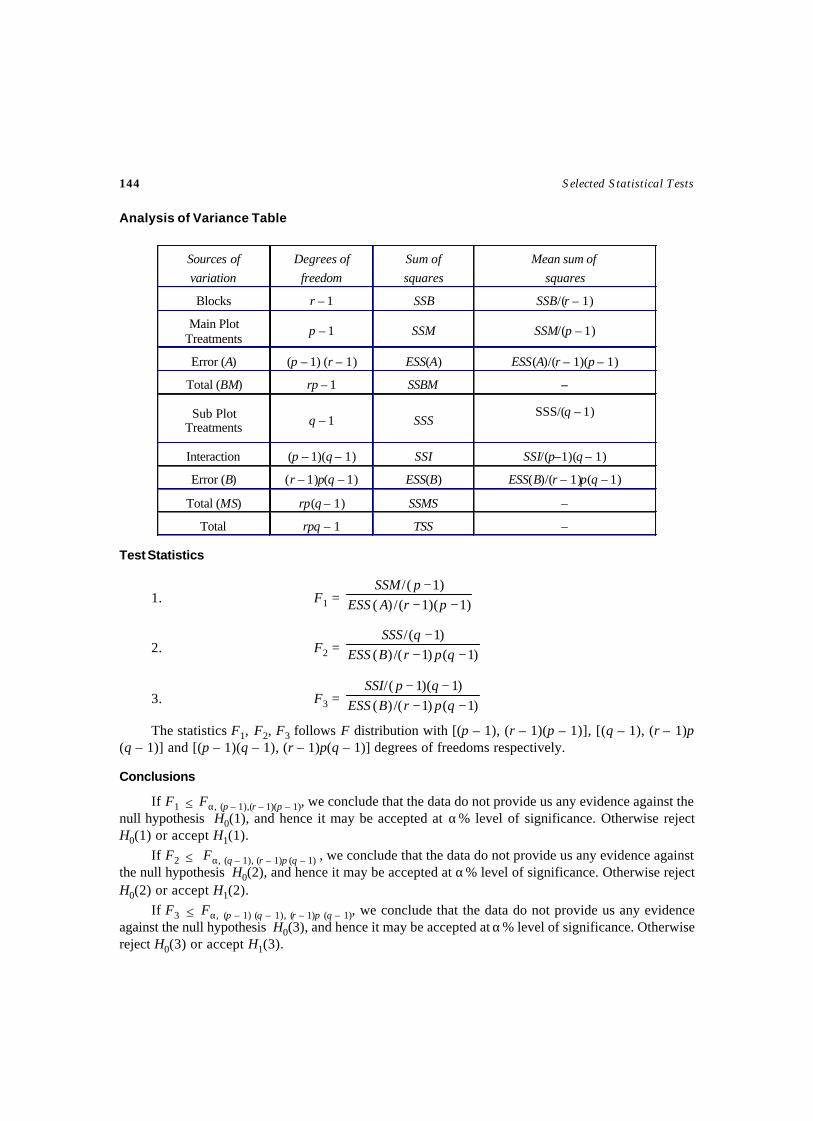
144 Selected Statistical Tests
Analysis of Variance Table
Test Statistics
1. F1 = )1)(1(/)()1(/
−−−
prAESSpSSM
2. F2 = )1()1(/)()1(/
−−−
qprBESSqSSS
3. F3 = )1()1(/)()1)(1(/−−
−−qprBESS
qpSSI
The statistics F1, F2, F3 follows F distribution with [(p – 1), (r – 1)(p – 1)], [(q – 1), (r – 1)p(q – 1)] and [(p – 1)(q – 1), (r – 1)p(q – 1)] degrees of freedoms respectively.
Conclusions
If F1 ≤ Fα, (p – 1),(r – 1)(p – 1), we conclude that the data do not provide us any evidence against thenull hypothesis H0(1), and hence it may be accepted at α% level of significance. Otherwise rejectH0(1) or accept H1(1).
If F2 ≤ Fα, (q – 1), (r – 1)p (q – 1) , we conclude that the data do not provide us any evidence againstthe null hypothesis H0(2), and hence it may be accepted at α% level of significance. Otherwise rejectH0(2) or accept H1(2).
If F3 ≤ Fα, (p – 1) (q – 1), (r – 1)p (q – 1), we conclude that the data do not provide us any evidenceagainst the null hypothesis H0(3), and hence it may be accepted at α% level of significance. Otherwisereject H0(3) or accept H1(3).
Sources of
variation
Degrees of
freedom
Sum of
squares
Mean sum of
squares
Blocks r – 1 SSB SSB/(r – 1)
Main Plot Treatments
p – 1 SSM SSM/(p – 1)
Error (A) (p – 1) (r – 1) ESS(A) ESS(A)/(r – 1)(p – 1)
Total (BM) rp – 1 SSBM –
Sub Plot Treatments q – 1 SSS
SSS/(q – 1)
Interaction (p – 1)(q – 1) SSI SSI/(p–1)(q – 1)
Error (B) (r – 1)p(q – 1) ESS(B) ESS(B)/(r – 1)p(q – 1)
Total (MS) rp(q – 1) SSMS –
Total rpq – 1 TSS –
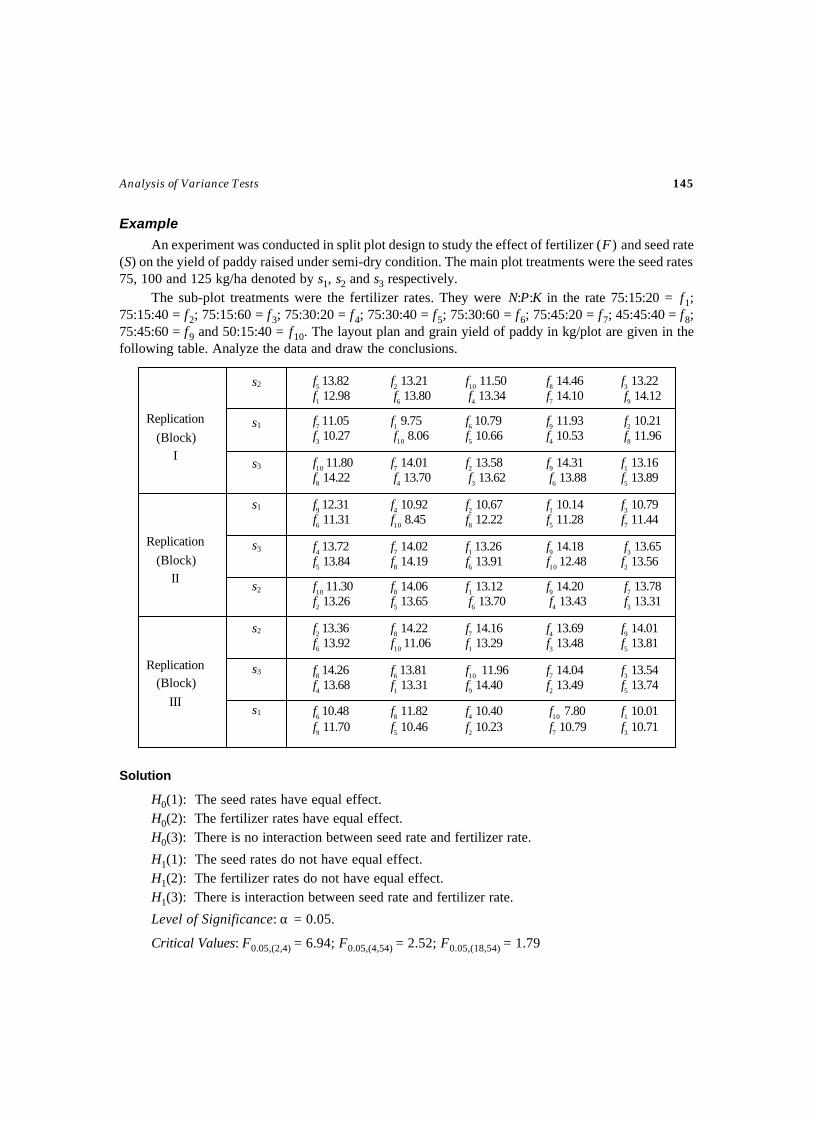
Analysis of Variance Tests 145
Example
An experiment was conducted in split plot design to study the effect of fertilizer (F ) and seed rate(S) on the yield of paddy raised under semi-dry condition. The main plot treatments were the seed rates75, 100 and 125 kg/ha denoted by s1, s2 and s3 respectively.
The sub-plot treatments were the fertilizer rates. They were N:P:K in the rate 75:15:20 = f1;75:15:40 = f2; 75:15:60 = f3; 75:30:20 = f4; 75:30:40 = f5; 75:30:60 = f6; 75:45:20 = f7; 45:45:40 = f8;75:45:60 = f9 and 50:15:40 = f10. The layout plan and grain yield of paddy in kg/plot are given in thefollowing table. Analyze the data and draw the conclusions.
Solution
H0(1): The seed rates have equal effect.H0(2): The fertilizer rates have equal effect.H0(3): There is no interaction between seed rate and fertilizer rate.
H1(1): The seed rates do not have equal effect.H1(2): The fertilizer rates do not have equal effect.H1(3): There is interaction between seed rate and fertilizer rate.
Level of Significance: α = 0.05.
Critical Values: F0.05,(2,4) = 6.94; F0.05,(4,54) = 2.52; F0.05,(18,54) = 1.79
s2
s1
Replication
(Block) I
s3
s1
s3
Replication
(Block) II
s2
s2
s3
Replication (Block)
III
s1
f5 13.82 f2 13.21 f10 11.50 f8 14.46 f3 13.22f1 12.98 f6 13.80 f4 13.34 f7 14.10 f9 14.12
f7 11.05 f1 9.75 f6 10.79 f9 11.93 f2 10.21f3 10.27 f10 8.06 f5 10.66 f4 10.53 f8 11.96
f10 11.80 f7 14.01 f2 13.58 f9 14.31 f1 13.16f8 14.22 f4 13.70 f3 13.62 f6 13.88 f5 13.89
f9 12.31 f4 10.92 f2 10.67 f1 10.14 f3 10.79f6 11.31 f10 8.45 f8 12.22 f5 11.28 f7 11.44
f4 13.72 f7 14.02 f1 13.26 f9 14.18 f3 13.65f5 13.84 f8 14.19 f6 13.91 f10 12.48 f2 13.56
f10 11.30 f8 14.06 f1 13.12 f9 14.20 f7 13.78f2 13.26 f5 13.65 f6 13.70 f4 13.43 f3 13.31
f2 13.36 f8 14.22 f7 14.16 f4 13.69 f9 14.01f6 13.92 f10 11.06 f1 13.29 f3 13.48 f5 13.81
f8 14.26 f6 13.81 f10 11.96 f7 14.04 f3 13.54f4 13.68 f1 13.31 f9 14.40 f2 13.49 f5 13.74
f6 10.48 f8 11.82 f4 10.40 f10 7.80 f1 10.01f9 11.70 f5 10.46 f2 10.23 f7 10.79 f3 10.71
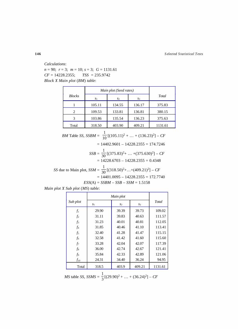
146 Selected Statistical Tests
≠≠≠
≠
Calculations:n = 90; r = 3; m = 10; s = 3; G = 1131.61CF = 14228.2355; TSS = 235.9742Block X Main plot (BM) table:
BM Table SS, SSBM = 101
[(105.11)2 + … + (136.23)2] – CF
= 14402.9601 – 14228.2355 = 174.7246
SSB = 301
[(375.83)2+ … +(375.630)2] – CF
= 14228.6703 – 14228.2355 = 0.4348
SS due to Main plot, SSM = 301
[(318.50)2+…+(409.21)2] – CF
= 14401.0095 – 14228.2355 = 172.7740ESS(A) = SSBM – SSB – SSM = 1.5158
Main plot X Sub plot (MS) table:
MS table SS, SSMS = 31
[(29.90)2 + … + (36.24)2] – CF
Main plot (Seed rates)
Blocks s1 s2 s3
Total
1 105.11 134.55 136.17 375.83
2 109.53 133.81 136.81 380.15
3 103.86 135.54 136.23 375.63
Total 318.50 403.90 409.21 1131.61
Main plot Sub plot
s1 s2 s3
Total
f1
f2
f3 f4
f5 f6
f7 f8
f9 f10
29.90
31.11
31.23 31.85
32.40 32.58
33.28 36.00
35.84 24.31
39.39
39.83
40.01 40.46
41.28 41.42
42.04 42.74
42.33 34.40
39.73
40.63
40.81 41.10
41.47 41.60
42.07 42.67
42.89 36.24
109.02
111.57
112.05 113.41
115.15 115.60
117.39 121.41
121.06 94.95
Total 318.5 403.9 409.21 1131.61
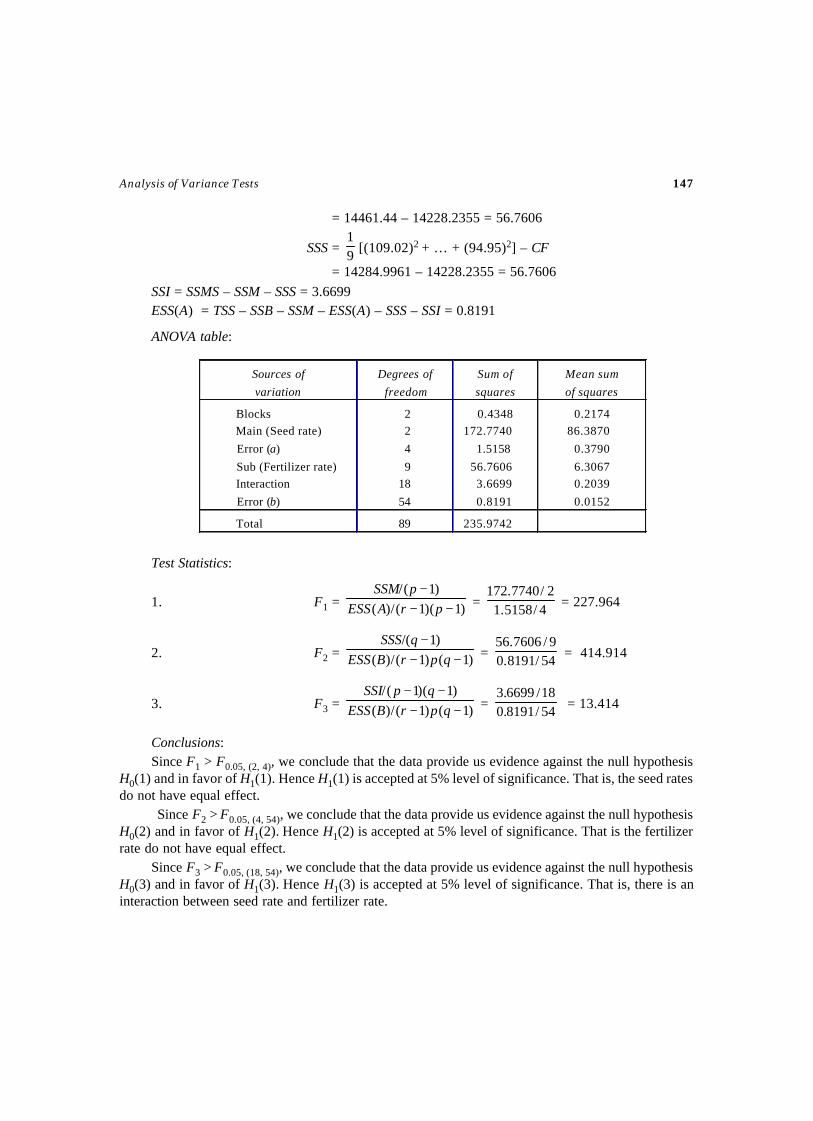
Analysis of Variance Tests 147
= 14461.44 – 14228.2355 = 56.7606
SSS = 91
[(109.02)2 + … + (94.95)2] – CF
= 14284.9961 – 14228.2355 = 56.7606SSI = SSMS – SSM – SSS = 3.6699ESS(A) = TSS – SSB – SSM – ESS(A) – SSS – SSI = 0.8191
ANOVA table:
Test Statistics:
1. F1 = )1)(1(/)()1(/
−−−
prAESSpSSM
= 4/5158.12/7740.172
= 227.964
2. F2 = )1()1(/)()1(/
−−−
qprBESSqSSS
= 54/8191.09/7606.56
= 414.914
3. F3 = )1()1(/)()1)(1(/−−
−−qprBESS
qpSSI = 54/8191.0
18/6699.3 = 13.414
Conclusions:Since F1 > F0.05, (2, 4), we conclude that the data provide us evidence against the null hypothesis
H0(1) and in favor of H1(1). Hence H1(1) is accepted at 5% level of significance. That is, the seed ratesdo not have equal effect.
Since F2 > F0.05, (4, 54), we conclude that the data provide us evidence against the null hypothesisH0(2) and in favor of H1(2). Hence H1(2) is accepted at 5% level of significance. That is the fertilizerrate do not have equal effect.
Since F3 > F0.05, (18, 54), we conclude that the data provide us evidence against the null hypothesisH0(3) and in favor of H1(3). Hence H1(3) is accepted at 5% level of significance. That is, there is aninteraction between seed rate and fertilizer rate.
Sources of
variation
Degrees of
freedom
Sum of
squares
Mean sum
of squares
Blocks Main (Seed rate)
Error (a)
Sub (Fertilizer rate) Interaction
Error (b)
2 2
4
9 18
54
0.4348 172.7740
1.5158
56.7606 3.6699
0.8191
0.2174 86.3870
0.3790
6.3067 0.2039
0.0152
Total 89 235.9742
≠≠≠
≠

ANOVA TEST FOR STRIP PLOT DESIGN
TEST – 35
Aim
To test the significance of the effect of main plot treatments and the effect of sub plot treatmentsbased on strip plot design.
Source
In this design, the main plot treatments are applied at random to rows and the sub plot treatmentsare applied at random to columns. Suppose we are interested to test two factors ‘a’ and ‘b’, factor ‘a’being at p levels a1, a2, …, ap and factor ‘b’ at q levels b1, b2, …, bq as in split plot design.
Hence, there are p main plot treatments, q sub plot treatments and r replications (blocks), so thatthere are rpq = n experimental units in total. The observations are arranged in a three-way table.
Linear Model
The model for this experiment isYijk = µ + ri + mj + mij + sk + eik + δjk + εijk
(i = 1, 2, …, r ; j = 1, 2,…, p ; k = 1, 2,…, q)
WhereYijk is the observation of the ith block, jth main plot and kth sub plot.µ is the overall mean effect.ri is the effect due to the ith block.mj is the effect due to the jth main plot treatment.mij is the main plot error or error (A).sk is the effect due to the kth sub plot treatment.δjk is the effect due to interaction between main and sub plots.
Analysis of Variance Tests 149
and εijk is the error effect due to sub plot and interaction or error (B).
Assumptions
1. The main plot treatments are allocated randomly to each rows of the block.2. The sub plot treatments are allocated randomly to each columns of the block.3. ri, mij, eik and eijk are independently normally distributed each with mean zero and variance
…σ…σ…σ 22 , emr and 2εσ respectively..
4. ∑j
jm = 0, ∑k
ks = 0, ,0=δ∑k
jk … ∀ . j, ∑δj
jk = 0 …∀ . k.
Null Hypotheses
H0(1): The m main plot treatments have equal effect. i.e., H0(1): m1 = m2 = …, = mp.H0(2): The s sub plot treatments have equal effect. i.e., H0(2): s1 = s2 = …, = sq.H0(3): There is no interaction between main and sub plot treatments. i.e., H0(3): δjk = 0 for all j
and k.
Alternative Hypotheses
H1(1): The m main plot treatments do not have equal effect. i.e., H1(1): m1 ≠ m2 ≠ …, ≠ mp.H1(2): The s sub plot treatments do not have equal effect. i.e., H1(2): s1 ≠ s2 …, sq.H1(3): There is interaction between main and sub plot treatments. i.e., H1(3): δjk ≠ 0 for all j
and k.
Level of Significance ( αα) and Critical Region
F1 > Fα, (p – 1), (r – 1)(p – 1) such that P [F1 > Fα, (p – 1), (r – 1)(p – 1)] = αF2 > Fα, (q – 1), (r – 1)(q – 1) such that P [F2 > Fα, (q – 1), (r – 1)(q – 1)] = αF3 > Fα, (p – 1)(q – 1), (r – 1)(q – 1) such that P [F3 > Fα,(p – 1)(q – 1), (r – 1)(q – 1)] = αThe critical values of F at level of Significance α and for respective degrees of freedom, are
obtained from Table 4.
Method
Calculate the following, based on the observations:
Main Plot Analysis
1. Grand total of all the n observations, G = ∑∑∑= = =
r
i
p
j
q
kijky
1 1 1
2. Correction Factor, CF =n
G 2
3. Total Sum of Squares, TSS = ∑∑∑= = =
r
i
p
j
q
kijky
1 1 1
2
– CF
4. Form a two-way table (BM table) for Block × Main plot treatments as follows.
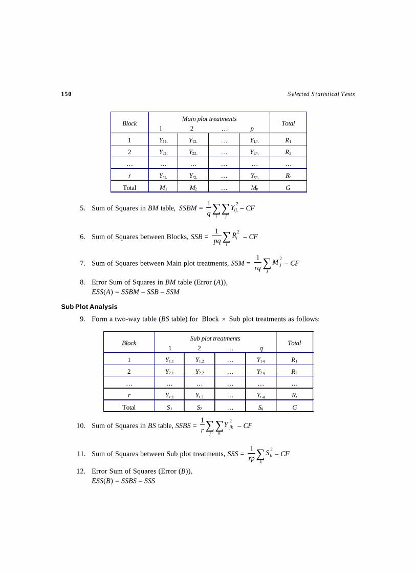
150 Selected Statistical Tests
5. Sum of Squares in BM table, SSBM = ∑∑i j
ijYq
2.
1– CF
6. Sum of Squares between Blocks, SSB = ∑i
iRpq
21 – CF
7. Sum of Squares between Main plot treatments, SSM = ∑j
jMrq
21– CF
8. Error Sum of Squares in BM table (Error (A)),ESS(A) = SSBM – SSB – SSM
Sub Plot Analysis
9. Form a two-way table (BS table) for Block × Sub plot treatments as follows:
10. Sum of Squares in BS table, SSBS = ∑∑j k
jkYr
2.
1 – CF
11. Sum of Squares between Sub plot treatments, SSS = ∑k
kSrp
21– CF
12. Error Sum of Squares (Error (B)),ESS(B) = SSBS – SSS
Block Main plot treatments
1 2 … p Total
1 Y11. Y12. … Y1p. R1
2 Y21. Y22. … Y2p. R2
… … … … … …
r Yr1. Yr2. … Yrp. Rr
Total M1 M2 … Mp G
Block Sub plot treatments
1 2 … q Total
1 Y1.1 Y1.2 … Y1.q R1
2 Y2.1 Y2.2 … Y2.q R2
… … … … … …
r Yr.1 Yr.2 … Yr.q Rr
Total S1 S2 … Sq G
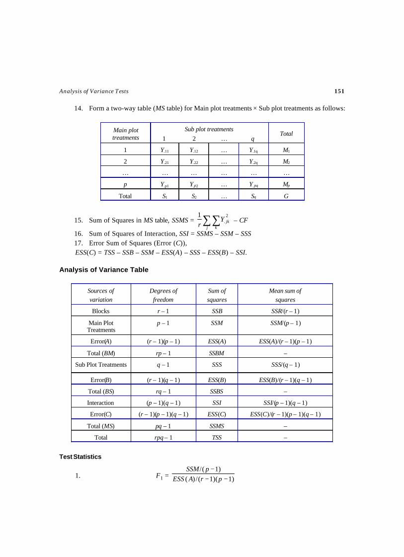
Analysis of Variance Tests 151
14. Form a two-way table (MS table) for Main plot treatments × Sub plot treatments as follows:
15. Sum of Squares in MS table, SSMS = ∑∑j k
jkYr
2.
1 – CF
16. Sum of Squares of Interaction, SSI = SSMS – SSM – SSS17. Error Sum of Squares (Error (C)),ESS(C) = TSS – SSB – SSM – ESS(A) – SSS – ESS(B) – SSI.
Analysis of Variance Table
Test Statistics
1. F1 = )1)(1(/)()1(/
−−−
prAESSpSSM
Main plot treatments
Sub plot treatments
1 2 … q Total
1 Y.11 Y.12 … Y.1q M1
2 Y.21 Y.22 … Y.2q M2
… … … … … …
p Y.p1 Y.p2 … Y.pq Mp
Total S1 S2 … Sq G
Sources of variation
Degrees of freedom
Sum of squares
Mean sum of squares
Blocks r – 1 SSB SSR/(r – 1)
Main Plot Treatments
p – 1 SSM SSM/(p – 1)
Error(A) (r – 1)(p – 1) ESS(A) ESS(A)/(r – 1)(p – 1)
Total (BM) rp – 1 SSBM –
Sub Plot Treatments q – 1 SSS SSS/(q – 1)
Error(B) (r – 1)(q – 1) ESS(B) ESS(B)/(r – 1)(q – 1)
Total (BS) rq – 1 SSBS –
Interaction (p – 1)(q – 1) SSI SSI/(p – 1)(q – 1)
Error(C) (r – 1)(p – 1)(q – 1) ESS(C) ESS(C)/(r – 1)(p – 1)(q – 1)
Total (MS) pq – 1 SSMS –
Total rpq – 1 TSS –
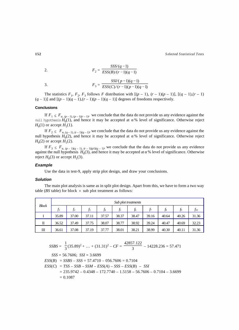
152 Selected Statistical Tests
2. F2 = )1)(1(/)()1(/
−−−
qrBESSqSSS
3. F3 = )1)(1)(1()()1)(1(
−−−−−
qpr/CESSqpSSI/
The statistics F1, F2, F3 follows F distribution with [(p – 1), (r – 1)(p – 1)], [(q – 1),(r – 1)(q – 1)] and [(p – 1)(q – 1),(r – 1)(p – 1)(q – 1)] degrees of freedoms respectively.
Conclusions
If F1 ≤ Fα, (p – 1), (p – 1)(r – 1), we conclude that the data do not provide us any evidence against thenull hypothesis H0(1), and hence it may be accepted at α% level of significance. Otherwise rejectH0(1) or accept H1(1).
If F2 ≤ Fα, (q – 1), (r – 1)(q – 1), we conclude that the data do not provide us any evidence against thenull hypothesis H0(2), and hence it may be accepted at α% level of significance. Otherwise rejectH0(2) or accept H1(2).
If F3 ≤ Fα, (p – 1)(q – 1), (r – 1)(p1)(q – 1), we conclude that the data do not provide us any evidenceagainst the null hypothesis H0(3), and hence it may be accepted at α% level of significance. Otherwisereject H0(3) or accept H1(3).
Example
Use the data in test-9, apply strip plot design, and draw your conclusions.
Solution
The main plot analysis is same as in split plot design. Apart from this, we have to form a two waytable (BS table) for block × sub plot treatment as follows:
SSBS = 31
(35.89)2 + … + (31.31)2 – CF = 3122.42857
– 14228.236 = 57.471
SSS = 56.7606; SSI = 3.6699ESS(B) = SSBS – SSS = 57.4710 – 056.7606 = 0.7104ESS(C) = TSS – SSB – SSM – ESS(A) – SSS – ESS(B) – SSI
= 235.9742 – 0.4348 – 172.7740 – 1.5158 – 56.7606 – 0.7104 – 3.6699= 0.1087
Sub plot treatments Block
f1 f2 f3 f4 f5 f6 f7 f8 f9 f10
I 35.89 37.00 37.11 37.57 38.37 38.47 39.16 40.64 40.26 31.36
II 36.52 37.49 37.75 38.07 38.77 38.92 39.24 40.47 40.69 32.23
III 36.61 37.08 37.19 37.77 38.01 38.21 38.99 40.30 40.11 31.36
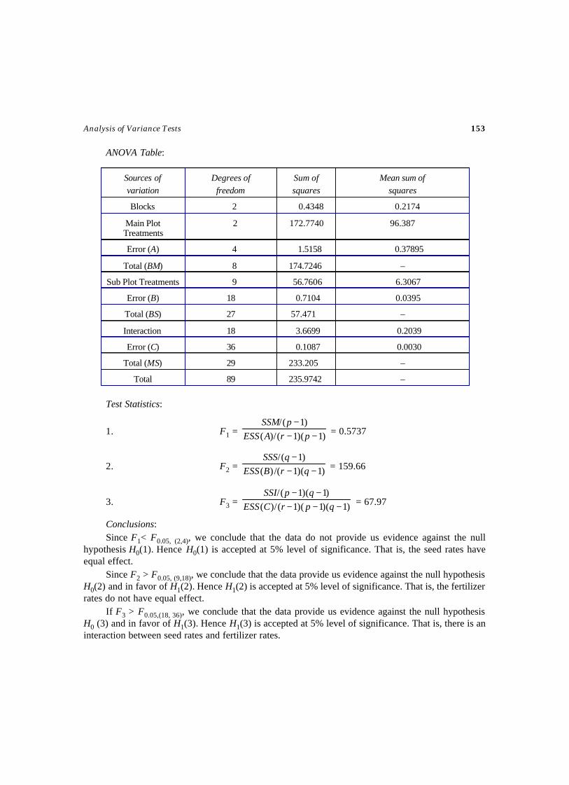
Analysis of Variance Tests 153
ANOVA Table:
Test Statistics:
1. F1 = )1)(1(/)()1(/
−−−
prAESSpSSM
= 0.5737
2. F2 = )1)(1(/)()1(/
−−−
qrBESSqSSS
= 159.66
3. F3 = )1)(1)(1(/)()1)(1(/
−−−−−
qprCESSqpSSI
= 67.97
Conclusions:Since F1< F0.05, (2,4), we conclude that the data do not provide us evidence against the null
hypothesis H0(1). Hence H0(1) is accepted at 5% level of significance. That is, the seed rates haveequal effect.
Since F2 > F0.05, (9,18), we conclude that the data provide us evidence against the null hypothesisH0(2) and in favor of H1(2). Hence H1(2) is accepted at 5% level of significance. That is, the fertilizerrates do not have equal effect.
If F3 > F0.05,(18, 36), we conclude that the data provide us evidence against the null hypothesisH0 (3) and in favor of H1(3). Hence H1(3) is accepted at 5% level of significance. That is, there is aninteraction between seed rates and fertilizer rates.
Sources of variation
Degrees of freedom
Sum of squares
Mean sum of squares
Blocks 2 0.4348 0.2174
Main Plot Treatments
2 172.7740 96.387
Error (A) 4 1.5158 0.37895
Total (BM) 8 174.7246 –
Sub Plot Treatments 9 56.7606 6.3067
Error (B) 18 0.7104 0.0395
Total (BS) 27 57.471 –
Interaction 18 3.6699 0.2039
Error (C) 36 0.1087 0.0030
Total (MS) 29 233.205 –
Total 89 235.9742 –

This pageintentionally left
blank

MULTIVARIATE TESTS
CHAPTER – 4

This pageintentionally left
blank
TEST FOR POPULATION MEAN VECTOR(Covariance Matrix is Known)
TEST – 36
Aim
To test the mean vector of the multivariate population µ be regarded as µ0, based on a multivariaterandom sample. That is, to investigate the significance of the difference between the assumed populationmean vector µ0 and sample mean vector X .
Source
Let Xij, (i = 1, 2,…p; j = 1, 2,…, N) be a random sample of p-fold N observations drawn from ap-variate normal population whose mean vector µ = (µ1, µ2,…, µp)
T is unknown and co-variancematrix
Σ =
σσσ
σσσσσσ
pppp
p
p
...
............
...
...
21
22221
11211
is known
The diagonal elements of Σ are variances, the non-diagonal elements are co-variances and the
matrix is symmetric. Let X = ( pXXX ,...,, 21 )T; ∑=
=N
jiji XX
1
; (i = 1, 2,…, p) be the sample mean
vector which is an unbiased estimate of the population mean vector µ.
Assumptions
(i) The population from which, the sample drawn, is p-variate normal population.(ii) The covariance matrix Σ is known.
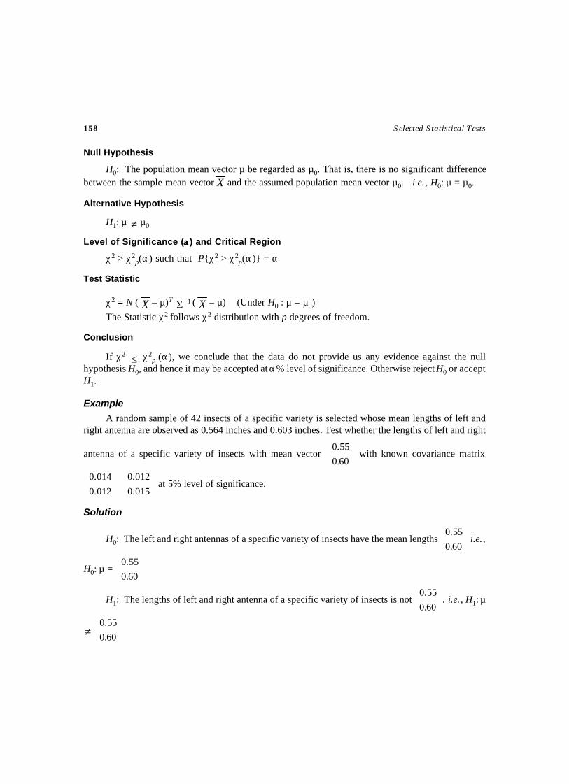
158 Selected Statistical Tests
Null Hypothesis
H0: The population mean vector µ be regarded as µ0. That is, there is no significant differencebetween the sample mean vector X and the assumed population mean vector µ0. i.e., H0: µ = µ0.
Alternative Hypothesis
H1: µ ≠ µ0
Level of Significance (αα) and Critical Region
χ2 > χ2p(α) such that P{χ2 > χ2
p(α)} = α
Test Statistic
χ2 = N ( X – µ)T 1−Σ ( X – µ) (Under H0 : µ = µ0)
The Statistic χ2 follows χ2 distribution with p degrees of freedom.
Conclusion
If χ2 ≤ χ2p (α), we conclude that the data do not provide us any evidence against the null
hypothesis H0, and hence it may be accepted at α% level of significance. Otherwise reject H0 or acceptH1.
Example
A random sample of 42 insects of a specific variety is selected whose mean lengths of left andright antenna are observed as 0.564 inches and 0.603 inches. Test whether the lengths of left and right
antenna of a specific variety of insects with mean vector
60.0
55.0 with known covariance matrix
015.0012.0
012.0014.0 at 5% level of significance.
Solution
H0: The left and right antennas of a specific variety of insects have the mean lengths
60.0
55.0 i.e.,
H0: µ =
60.0
55.0
H1: The lengths of left and right antenna of a specific variety of insects is not
60.0
55.0. i.e., H1: µ
≠
60.0
55.0
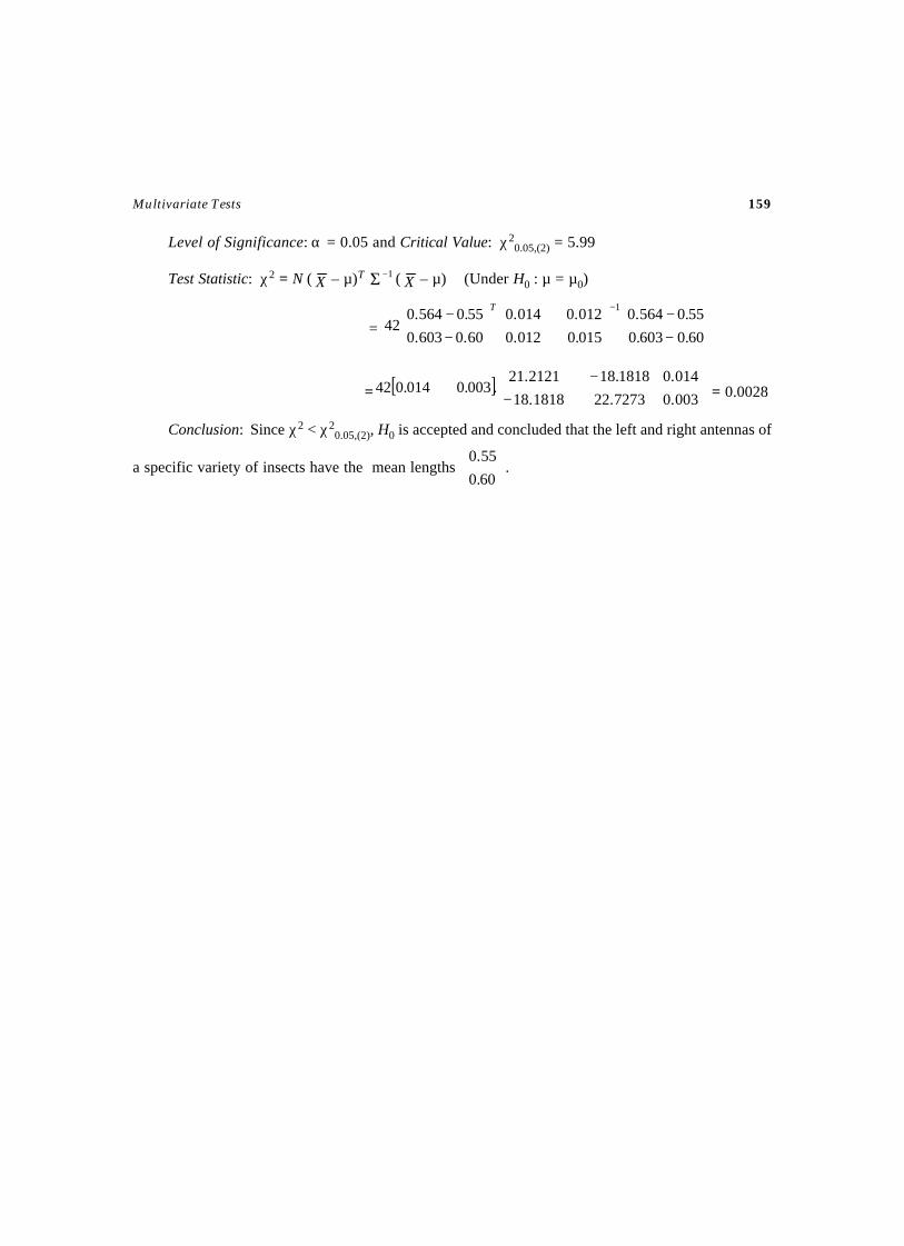
Multivariate Tests 159
Level of Significance: α = 0.05 and Critical Value: χ20.05,(2) = 5.99
Test Statistic: χ2 = N ( X – µ)T 1−Σ ( X – µ) (Under H0 : µ = µ0)
=
−−
−− −
60.0603.0
55.0564.0
015.0012.0
012.0014.0
60.0603.0
55.0564.042
1T
= [ ]
−
−003.0
014.0
7273.221818.18
1818.182121.21.003.0014.042 = 0.0028
Conclusion: Since χ2 < χ20.05,(2), H0 is accepted and concluded that the left and right antennas of
a specific variety of insects have the mean lengths
60.0
55.0.
Aim
To test the null hypothesis that the mean vector of the multivariate population µ be regarded as µ0,based a multivariate random sample. That is, to investigate the significance of the difference betweenthe assumed population mean vector µ0 and the sample mean vector X .
Source
Let Xij, (i = 1, 2,…p ; j = 1, 2,…, N) be a sample of p-fold N observations drawn from a p-variatenormal population whose mean vector µ = (µ1, µ2,…, µp)
T and the covariance matrix Σ are unknown.
Let X = T
pXXX )...,,,( 21 be the sample mean vector which is an unbiased estimate of the populationmean vector µ. The unknown covariance matrix Σ is estimated by
S =1–N
A
A = ( )( )∑=
−−N
j
Tijij XXXX
1
S =
pppp
p
p
SSS
SSS
SSS
...
............
...
...
21
22221
11211
The diagonal elements of S are variances, the non-diagonal elements are co-variances, and thematrix is symmetric.
TEST FOR POPULATION MEAN VECTOR(Covariance Matrix is Unknown)
TEST – 37
Multivariate Tests 161
Assumptions
(i) The population from which, the sample drawn is p-variate normal population.(ii) The covariance matrix Σ is unknown.
Null Hypothesis
H0: The population mean vector µ be regarded as µ0. That is, there is no significant differencebetween the sample mean vector X and the assumed population mean vector µ0. i.e., H0: µ = µ0.
Alternative Hypothesis
H1: µ ≠ µ0
Level of Significance (αα) and Critical Region
F > Fp,N–p(α) such that P{F > Fp,N–p(α)} = α
Test Statistic
2T = N ( X – µ)T S–1( X – µ) (Under H0 : µ = µ0)
1–
2
NT = N )–( 0µX T A–1 )–( 0µX
and F =p
pNNT –
1–
2
The Statistic F follows F distribution with (p, N–p) degrees of freedom.
Conclusion
If F ≤ Fp,N–p(α), we conclude that the data do not provide us any evidence against the nullhypothesis H0, and hence it may be accepted at α% level of significance. Otherwise reject H0 or acceptH1.
Note: This test is also known as Hotelling’s T2 test.
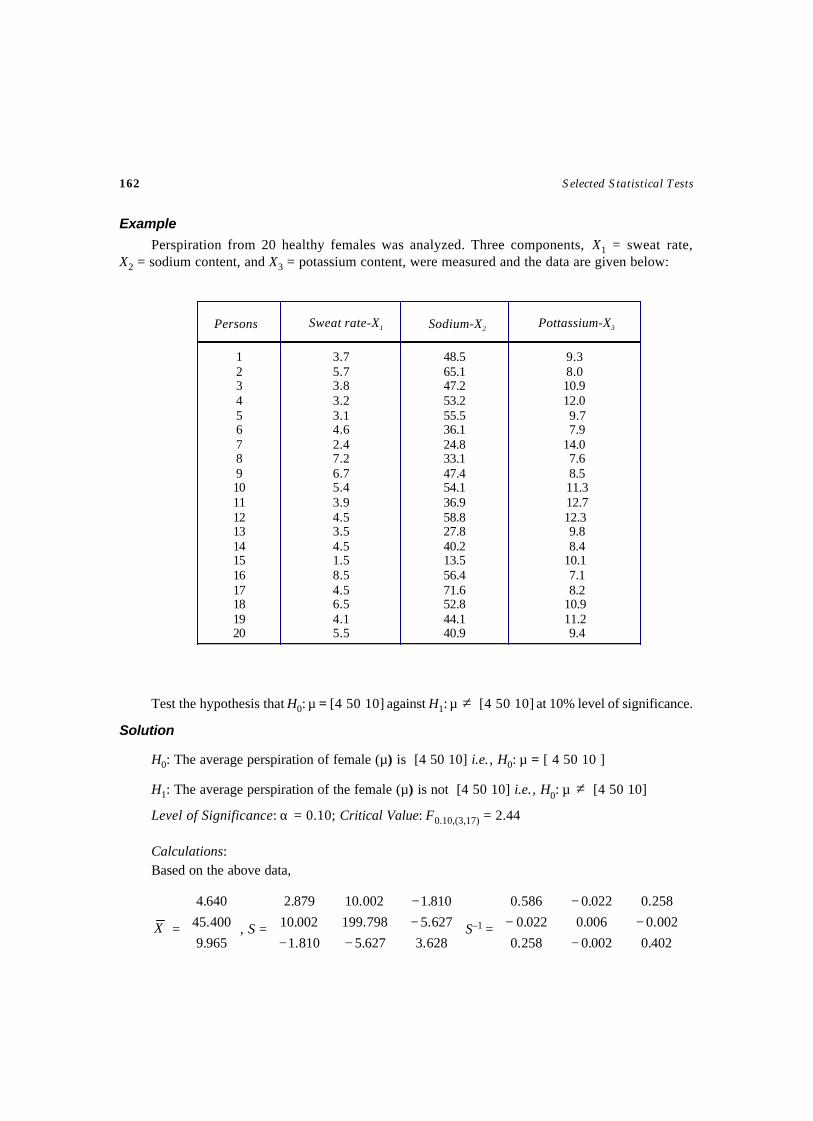
162 Selected Statistical Tests
Example
Perspiration from 20 healthy females was analyzed. Three components, X1 = sweat rate,X2 = sodium content, and X3 = potassium content, were measured and the data are given below:
Test the hypothesis that H0: µ = [4 50 10] against H1: µ ≠ [4 50 10] at 10% level of significance.
Solution
H0: The average perspiration of female (µ) is [4 50 10] i.e., H0: µ = [ 4 50 10 ]
H1: The average perspiration of the female (µ) is not [4 50 10] i.e., H0: µ ≠ [4 50 10]
Level of Significance: α = 0.10; Critical Value: F0.10,(3,17) = 2.44
Calculations:Based on the above data,
X =
965.9
400.45
640.4
, S =
−−−−
628.3627.5810.1
627.5798.199002.10
810.1002.10879.2
S–1 =
−−−
−
402.0002.0258.0
002.0006.0022.0
258.0022.0586.0
1 2 3 4 5 6 7 8 9 10 11 12 13 14 15 16 17 18 19 20
3.7 5.7 3.8 3.2 3.1 4.6 2.4 7.2 6.7 5.4 3.9 4.5 3.5 4.5 1.5 8.5 4.5 6.5 4.1 5.5
48.5 65.1 47.2 53.2 55.5 36.1 24.8 33.1 47.4 54.1 36.9 58.8 27.8 40.2 13.5 56.4 71.6 52.8 44.1 40.9
9.3 8.0 10.9 12.0 9.7 7.9 14.0 7.6 8.5 11.3 12.7 12.3 9.8 8.4 10.1 7.1 8.2 10.9 11.2 9.4
Persons Sodium-X2Sweat rate-X1 Pottassium-X3
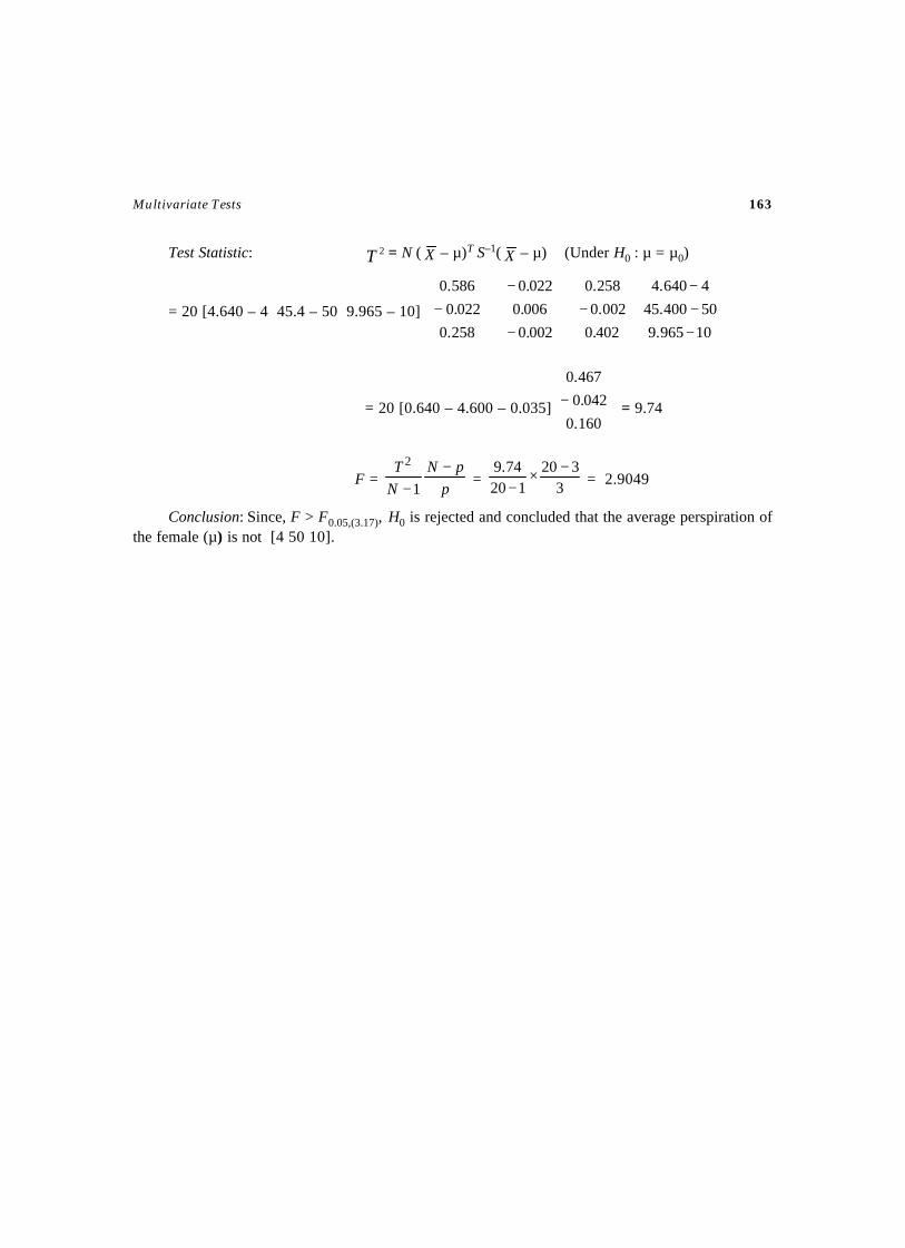
Multivariate Tests 163
Test Statistic: 2T = N ( X – µ)T S–1( X – µ) (Under H0 : µ = µ0)
= 20 [4.640 – 4 45.4 – 50 9.965 – 10]
−−−
−
402.0002.0258.0
002.0006.0022.0
258.0022.0586.0
−−−
10965.9
50400.45
4640.4
= 20 [0.640 – 4.600 – 0.035]
−
160.0
042.0
467.0
= 9.74
F =p
pNNT −
−1
2
= 3320
12074.9 −×− = 2.9049
Conclusion: Since, F > F0.05,(3.17), H0 is rejected and concluded that the average perspiration ofthe female (µ) is not [4 50 10].
Aim
To test the mean vectors of two multivariate populations µ1 and µ2 are equal, based on twomultivariate random samples. That is, to investigate the significance of the difference between thesample mean vectors.
Source
Let Xij(1), (i = 1, 2,…p ; j = 1, 2,…, N1) be a random sample of p-fold N1 observations called as
sample-1 drawn from a p-variate normal population whose mean vector µ(1) = (µ1(1), µ2
(1),…, µp(1))T.
Let Xij(2), (i = 1, 2,…p ; j = 1, 2,…, N2) be a random sample of p-fold N2 observations called as
sample-2 drawn independently from another p-variate normal population whose mean vectorµ(2) = (µ1
(2), µ2(2), …, µp
(2))T. The mean vectors µ(1) and µ(2) are unknown. The covariance matrices ofthe two populations are equal and known and is denoted by
Σ =
σσσ
σσσσσσ
pppp
p
p
...
............
...
...
21
22221
11211
The diagonal elements of Σ are variances, the non-diagonal elements are co-variances and the
matrix is symmetric. Let. )1(X = ( )1()1(2
)1(1 ,,, pXXX … )T be the sample mean vector of the sample-1
which is an unbiased estimate of the population mean vector µ(1) and )2(X = ( )2()2(2
)2(1 ,,, pXXX … )T
be the sample mean vector of the sample-2 which is an unbiased estimate of the population meanvector µ(2).
TEST FOR EQUALITY OF POPULATIONMEAN VECTORS
(Covariance Matrices are Equal and Known)
TEST – 38
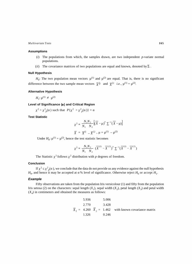
Multivariate Tests 165
Assumptions
(i) The populations from which, the samples drawn, are two independent p-variate normalpopulations.
(ii) The covariance matrices of two populations are equal and known, denoted by Σ .
Null Hypothesis
H0: The two population mean vectors µ(1) and µ(2) are equal. That is, there is no significant
difference between the two sample mean vectors ( )1X and ( )2X i.e., µ(1) = µ(2).
Alternative Hypothesis
H1: µ(1) ≠ µ(2)
Level of Significance (αα) and Critical Region
χ2 > χ2p(α) such that P{χ2 > χ2
p(α)} = α
Test Statistic
χ2 = [ ])()( 1
21
21 µ−∑µ−+
− XXNN
NN T
X = ( ) ( )21 – XX , µ = µ(1) – µ(2)
Under H0: µ(1) = µ(2), hence the test statistic becomes
χ2 =
−∑−
+− )()(
)2()1(1)2()1(
21
21 XXXXNN
NN T
The Statistic χ2 follows χ2 distribution with p degrees of freedom.
Conclusion
If χ2 ≤ χ2p(α), we conclude that the data do not provide us any evidence against the null hypothesis
H0, and hence it may be accepted at α% level of significance. Otherwise reject H0 or accept H1.
Example
Fifty observations are taken from the population Iris versicolour (1) and fifty from the populationIris setosa (2) on the characters: sepal length (X1), sepal width (X2), petal length (X3) and petal width(X4) in centimeters and obtained the measures as follows:
1X =
326.1
260.4
770.2
936.5
2X =
246.0
462.1
428.3
006.5
with known covariance matrix
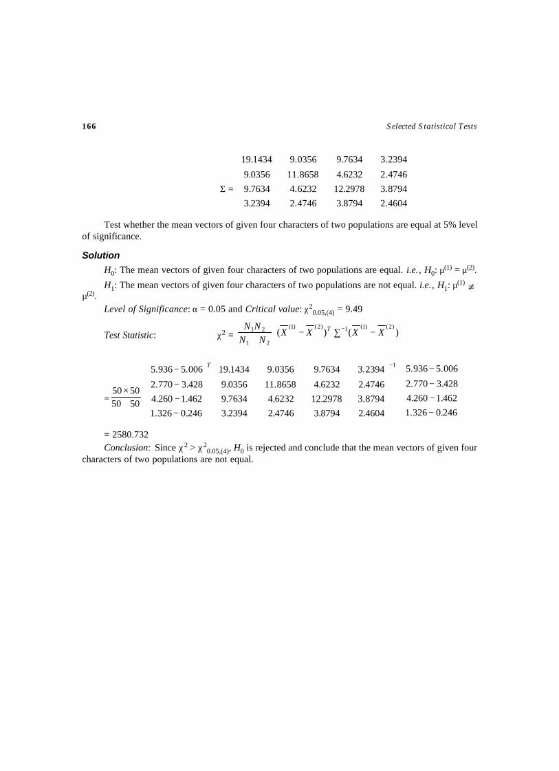
166 Selected Statistical Tests
Σ =
4604.28794.34746.22394.3
8794.32978.126232.47634.9
4746.26232.48658.110356.9
2394.37634.90356.91434.19
Test whether the mean vectors of given four characters of two populations are equal at 5% levelof significance.
Solution
H0: The mean vectors of given four characters of two populations are equal. i.e., H0: µ(1) = µ(2).
H1: The mean vectors of given four characters of two populations are not equal. i.e., H1: µ(1) ≠
µ(2).Level of Significance: α = 0.05 and Critical value: χ2
0.05,(4) = 9.49
Test Statistic: χ2 =
−∑−
+− )()(
)2()1(1)2()1(
21
21 XXXXNN
NN T
= 50505050
+×
T
−−−
−
246.0326.1
462.1260.4
428.3770.2
006.5936.5 1
4604.28794.34746.22394.3
8794.32978.126232.47634.9
4746.26232.48658.110356.9
2394.37634.90356.91434.19 −
−−−
−
246.0326.1
462.1260.4
428.3770.2
006.5936.5
= 2580.732Conclusion: Since χ2 > χ2
0.05,(4), H0 is rejected and conclude that the mean vectors of given fourcharacters of two populations are not equal.
Aim
To test the mean vectors of two multivariate populations µ1 and µ2 are equal, based on twomultivariate random samples. That is, to investigate the significance of the difference between the twosample mean vectors.
Source
Let Xij(1), (i = 1, 2, …p; j = 1, 2,…, N1) be a random sample of p-fold N1 observations called as
sample-1 drawn from a p-variate normal population whose mean vector µ(1) = (µ1(1), µ2
(1), …, µP(1))T.
Let Xij(2), (i = 1, 2,…p; j = 1, 2, …, N2) be a random sample of p-fold N2 observations called as
sample-2 drawn independently from another p-variate normal population whose mean vectorµ(2) = (µ1
(2), µ2(2),…, µp
(2))T. The mean vectors µ(1) and µ(2) are unknown. The covariance matrix of the
two populations is equal but unknown and is denoted by Σ . The estimate of Σ is given by
S = 21
21 −+ NN
−−+−− ∑∑==
21
1
)2()2()2()2(
1
)1()1()1()1( ))(())((N
j
Tijij
N
j
Tijij XXXXXXXX
S =
pppp
p
p
SSS
SSSSSS
...
............
...
...
21
22221
11211
The diagonal elements of S are variances, the non-diagonal elements are co-variances and the
matrix is symmetric. Let )1(X = ( )1()1(2
)1(1 ,,, pXXX … )T be the sample mean vector of the sample-1
which is an unbiased estimate of the population mean vector µ(1) and )2(X = ( )2()2(2
)2(1 ,,, pXXX … )T
be the sample mean vector of the sample-2 which is an unbiased estimate of the population meanvector µ(2).
TEST FOR EQUALITY OF POPULATIONMEAN VECTORS
(Covariance Matrices are Equal and Unknown)
TEST – 39
168 Selected Statistical Tests
Assumptions
(i) The populations from which, the sample drawn are two independent p-variate normalpopulations.
(ii) The covariance matrices of two populations are equal, denoted by Σ, is unknown.
Null Hypothesis
H0: The two population mean vectors µ(1) and µ(2) are equal. That is, there is no significant
difference between the two sample mean vectors )1(X and .)2(X i.e., H0: µ(1) = µ(2).
Alternative Hypothesis
H1: µ(1) ≠ µ(2)
Level of Significance (αα) and Critical Region
1––, 21 pNNpFF +> (α) such that P )}({ 1––, 21α> + pNNpFF = α
Test Statistic
T2 =21
21
NNNN
+( ) ( )
µ−µ− − XSX
T 1
X =)2()1(
XX − , µ = µ(1) – µ(2)
Under H0: µ(1) = µ(2), hence the test statistic becomes
T2 =21
21
NNNN
+
−
−
− )2()1(1)2()1(XXSXX
T
and F = ( ) ppNN
NNT 1
221
21
2 −−+−+
The Statistic F follows F distribution with (p1 N1 + N2 – p –1) degrees of freedom.
Conclusion
If 1––, 21 pNNpFF +≤ (α), we conclude that the data do not provide us any evidence against the
null hypothesis H0, and hence it may be accepted at α% level of significance. Otherwise reject H0 oraccept H1.
Note: This test is also known as Hotelling’s T2 test.
Example
Two random samples of sizes 45 and 55 were observed from Chennai city of households havingwith and without air conditioning, respectively. Two measurements of electrical usage (in kilowatthours) were considered. The first is the measure of total on peak consumption (X1) during July and thesecond is a measure of total off-peak consumption (X2) during July. The resulting summary statistics
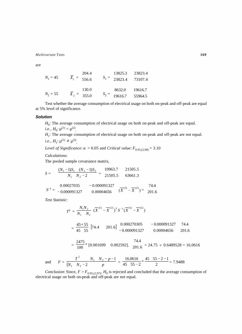
Multivariate Tests 169
are
N1 = 45 1X =
6.556
4.204S1 =
4.731074.23823
4.238233.13825
N2 = 55 2X =
0.355
0.130S2 =
5.559647.19616
7.196160.8632
Test whether the average consumption of electrical usage on both on-peak and off-peak are equalat 5% level of significance.
Solution
H0: The average consumption of electrical usage on both on-peak and off-peak are equal.i.e., H0: µ
(1) = µ(2).
H1: The average consumption of electrical usage on both on-peak and off-peak are not equal.
i.e., H1: µ(1) ≠ µ(2)
.
Level of Significance: α = 0.05 and Critical value: F0.05,(2,98) = 3.10
Calculations:The pooled sample covariance matrix,
S = 2)1()1(
21
2211
−+−+−
NNSNSN
=
3.636615.21505
5.215057.10963
S–1 =
−
−00004656.0000091327.0
000091327.000027035.0 )(
)2()1(XX − =
6.201
4.74
Test Statistic:
T2 =
−−
+− )()(
)2()1(1)2()1(
21
21 XXSXXNN
NN T
= [ ]
−
−+×
6.201
4.74
00004656.0000091327.0
000091327.0000270305.06.2014.74
55455545
= ×1002475
[0.001699 0.002592].
6.201
4.74= 24.75 × 0.6489528 = 16.0616
and F = ( ) ppNN
NNT 1
221
21
2 −−+−+
= 2125545
255450616.16 −−+×
−+ = 7.9488
Conclusion: Since, F > F0.05,(2,97), H0 is rejected and concluded that the average consumption ofelectrical usage on both on-peak and off-peak are not equal.
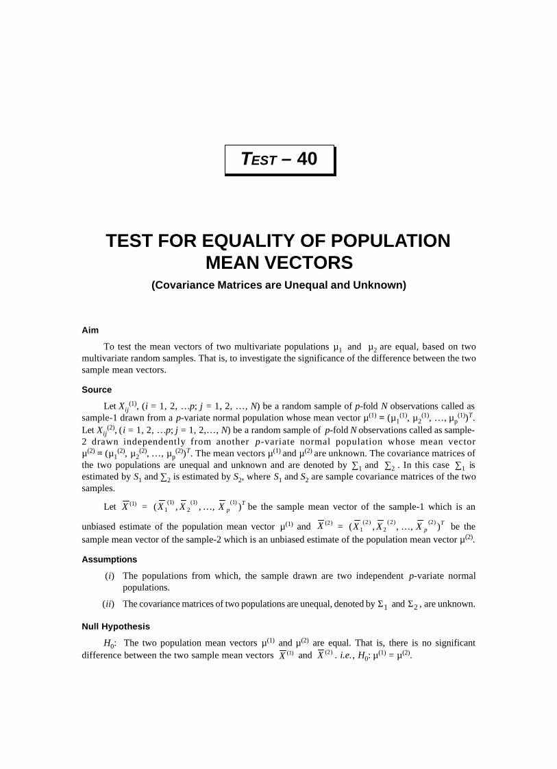
Aim
To test the mean vectors of two multivariate populations µ1 and µ2 are equal, based on twomultivariate random samples. That is, to investigate the significance of the difference between the twosample mean vectors.
Source
Let Xij(1), (i = 1, 2, …p; j = 1, 2, …, N) be a random sample of p-fold N observations called as
sample-1 drawn from a p-variate normal population whose mean vector µ(1) = (µ1(1), µ2
(1), …, µp(1))T.
Let Xij(2), (i = 1, 2, …p; j = 1, 2,…, N) be a random sample of p-fold N observations called as sample-
2 drawn independently from another p-variate normal population whose mean vectorµ(2) = (µ1
(2), µ2(2), …, µp
(2))T. The mean vectors µ(1) and µ(2) are unknown. The covariance matrices ofthe two populations are unequal and unknown and are denoted by ∑1 and ∑2 . In this case ∑1 isestimated by S1 and ∑2 is estimated by S2, where S1 and S2 are sample covariance matrices of the twosamples.
Let )1(X = TpXXX ),,,( )1()1(
2)1(
1 … be the sample mean vector of the sample-1 which is an
unbiased estimate of the population mean vector µ(1) and )2(X = TpXXX ),,,( )2()2(
2)2(
1 … be thesample mean vector of the sample-2 which is an unbiased estimate of the population mean vector µ(2).
Assumptions
(i) The populations from which, the sample drawn are two independent p-variate normalpopulations.
(ii) The covariance matrices of two populations are unequal, denoted by 1Σ and 2Σ , are unknown.
Null Hypothesis
H0: The two population mean vectors µ(1) and µ(2) are equal. That is, there is no significantdifference between the two sample mean vectors )1(X and )2(X . i.e., H0: µ
(1) = µ(2).
TEST FOR EQUALITY OF POPULATIONMEAN VECTORS
(Covariance Matrices are Unequal and Unknown)
TEST – 40
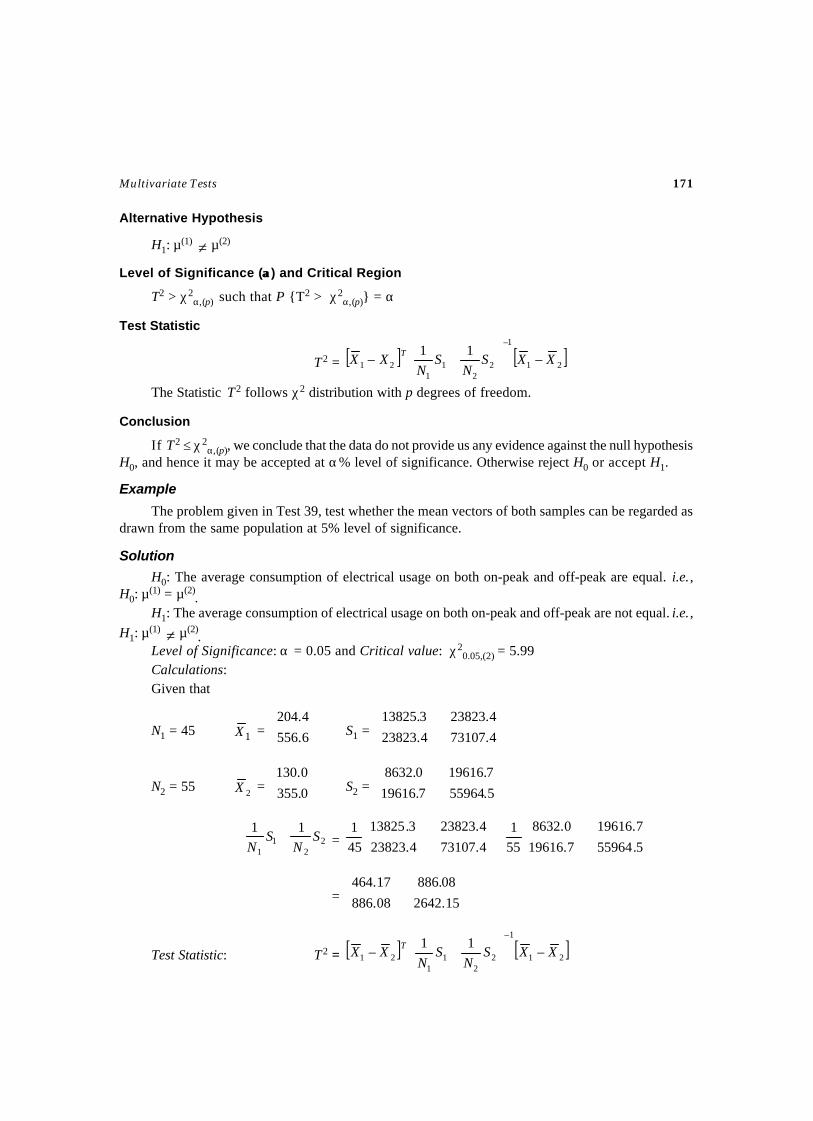
Multivariate Tests 171
Alternative Hypothesis
H1: µ(1) ≠ µ(2)
Level of Significance (αα) and Critical Region
T2 > χ2α,(p) such that P {T2 > χ2
α,(p)} = α
Test Statistic
T2 = [ ] [ ]21
1–
22
11
21 –11
– XXSN
SN
XX T
+
The Statistic T2 follows χ2 distribution with p degrees of freedom.
Conclusion
If T2 ≤ χ2α,(p), we conclude that the data do not provide us any evidence against the null hypothesis
H0, and hence it may be accepted at α% level of significance. Otherwise reject H0 or accept H1.
Example
The problem given in Test 39, test whether the mean vectors of both samples can be regarded asdrawn from the same population at 5% level of significance.
Solution
H0: The average consumption of electrical usage on both on-peak and off-peak are equal. i.e.,H0: µ
(1) = µ(2).
H1: The average consumption of electrical usage on both on-peak and off-peak are not equal. i.e.,H1: µ
(1) ≠ µ(2).
Level of Significance: α = 0.05 and Critical value: χ20.05,(2) = 5.99
Calculations:Given that
N1 = 45 1X =
6.556
4.204S1 =
4.731074.23823
4.238233.13825
N2 = 55 2X =
0.355
0.130S2 =
5.559647.19616
7.196160.8632
22
11
11S
NS
N+ =
+
5.559647.19616
7.196160.8632
551
4.731074.23823
4.238233.13825
451
=
15.264208.886
08.88617.464
Test Statistic: T2 = [ ] [ ]21
1–
22
11
21 –11
– XXSN
SN
XX T
+
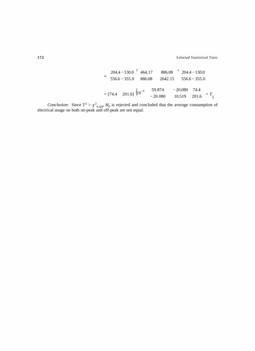
172 Selected Statistical Tests
=
−−
−− −
0.3556.556
0.1304.204
15.264208.886
08.88617.464
0.3556.556
0.1304.204 1T
= [74.4 201.6] ( )
−
−⋅−
6.201
4.74
519.10080.20
080.20874.5910 4
= T1
Conclusion: Since T2 > χ2α,(p), H0 is rejected and concluded that the average consumption of
electrical usage on both on-peak and off-peak are not equal.

NON–PARAMETRIC TESTS
CHAPTER – 5

This pageintentionally left
blank
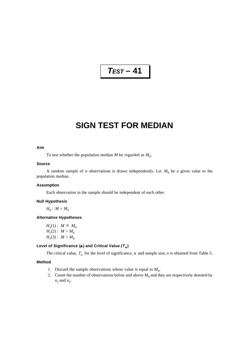
Aim
To test whether the population median M be regarded as M0.
Source
A random sample of n observations is drawn independently. Let M0 be a given value to thepopulation median.
Assumption
Each observation in the sample should be independent of each other.
Null Hypothesis
H0 : M = M0
Alternative Hypotheses
H1(1) : M ≠ M0H1(2) : M > M0
H1(3) : M < M0
Level of Significance (αα) and Critical Value (T αα )
The critical value, Tα for the level of significance, α and sample size, n is obtained from Table 5.
Method
1. Discard the sample observations whose value is equal to M0.2. Count the number of observations below and above M0 and they are respectively denoted by
n1 and n2.
SIGN TEST FOR MEDIAN
TEST – 41
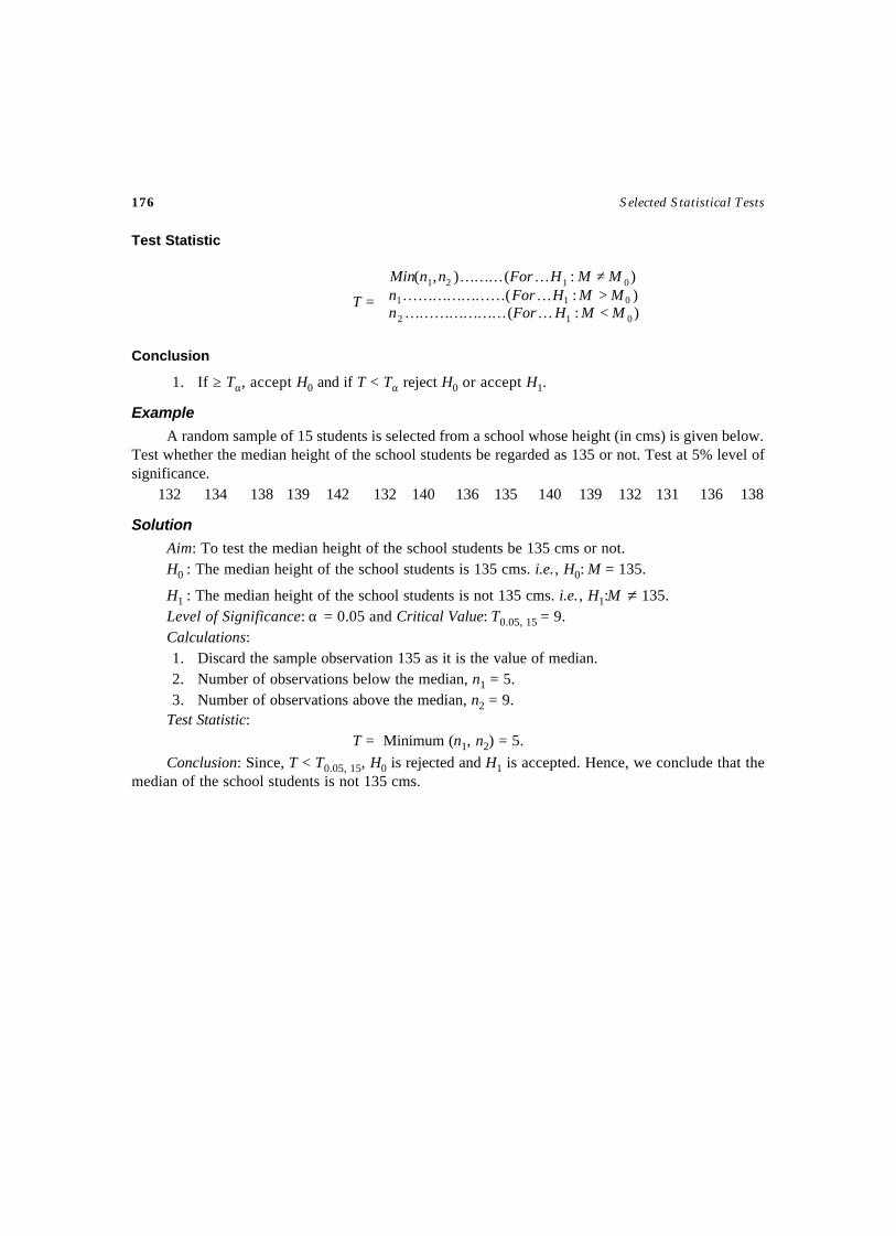
176 Selected Statistical Tests
Test Statistic
T =
<>≠
):():():(),(
012
011
0121
MMHFornMMHFornMMHFornnMin
……………………………………………………
Conclusion
1. If ≥ Tα, accept H0 and if T < Tα reject H0 or accept H1.
Example
A random sample of 15 students is selected from a school whose height (in cms) is given below.Test whether the median height of the school students be regarded as 135 or not. Test at 5% level ofsignificance.
132 134 138 139 142 132 140 136 135 140 139 132 131 136 138
Solution
Aim: To test the median height of the school students be 135 cms or not.H0 : The median height of the school students is 135 cms. i.e., H0: M = 135.
H1 : The median height of the school students is not 135 cms. i.e., H1:M ≠ 135.Level of Significance: α = 0.05 and Critical Value: T0.05, 15 = 9.Calculations:1. Discard the sample observation 135 as it is the value of median.2. Number of observations below the median, n1 = 5.3. Number of observations above the median, n2 = 9.
Test Statistic:T = Minimum (n1, n2) = 5.
Conclusion: Since, T < T0.05, 15, H0 is rejected and H1 is accepted. Hence, we conclude that themedian of the school students is not 135 cms.
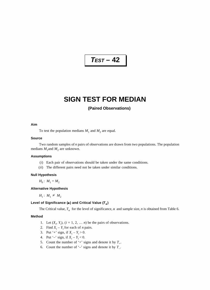
Aim
To test the population medians M1 and M2 are equal.
Source
Two random samples of n pairs of observations are drawn from two populations. The populationmedians M1and M2 are unknown.
Assumptions
(i) Each pair of observations should be taken under the same conditions.(ii) The different pairs need not be taken under similar conditions.
Null Hypothesis
H0 : M1 = M2
Alternative Hypothesis
H1 : M1 ≠ M2
Level of Significance (αα) and Critical Value (T αα )
The Critical value, Tα for the level of significance, α and sample size, n is obtained from Table 6.
Method
1. Let (Xi, Yi), (i = 1, 2, … n) be the pairs of observations.2. Find Xi – Yi for each of n pairs.3. Put ‘+’ sign, if Xi – Yi > 0.4. Put ‘–’ sign, if Xi – Yi < 0.5. Count the number of ‘+’ signs and denote it by T+.6. Count the number of ‘–’ signs and denote it by T–.
SIGN TEST FOR MEDIAN(Paired Observations)
TEST – 42
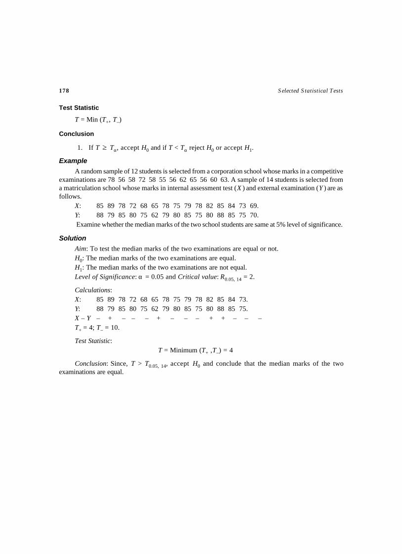
178 Selected Statistical Tests
Test Statistic
T = Min (T+, T–)
Conclusion
1. If T ≥ Tα, accept H0 and if T < Tα reject H0 or accept H1.
Example
A random sample of 12 students is selected from a corporation school whose marks in a competitiveexaminations are 78 56 58 72 58 55 56 62 65 56 60 63. A sample of 14 students is selected froma matriculation school whose marks in internal assessment test (X ) and external examination (Y ) are asfollows.
X: 85 89 78 72 68 65 78 75 79 78 82 85 84 73 69.Y: 88 79 85 80 75 62 79 80 85 75 80 88 85 75 70. Examine whether the median marks of the two school students are same at 5% level of significance.
Solution
Aim: To test the median marks of the two examinations are equal or not.H0: The median marks of the two examinations are equal.H1: The median marks of the two examinations are not equal.Level of Significance: α = 0.05 and Critical value: R0.05, 14 = 2.
Calculations:X: 85 89 78 72 68 65 78 75 79 78 82 85 84 73.Y: 88 79 85 80 75 62 79 80 85 75 80 88 85 75.X – Y – + – – – + – – – + + – – –T+ = 4; T– = 10.
Test Statistic:T = Minimum (T+ ,T–) = 4
Conclusion: Since, T > T0.05, 14, accept H0 and conclude that the median marks of the twoexaminations are equal.
Aim
To test the two samples are drawn from the populations having the same medians.
Source
A random sample of n1 observations, arranged in order of magnitude as, X1, X2,…, Xn1 drawnfrom a population with density function f1(.) and a random sample of n2 observations, arranged inorder of magnitude as, Y1, Y2,…, Yn2 drawn from another population with density function f2(.). Thepopulation medians of the two populations are unknown. Let N = n1 + n2.
Assumptions
(i) The two samples drawn are independent.(ii) The observations must be at least ordinal.
(iii) The sample sizes should be sufficiently large.
Null Hypothesis
H0: The two samples are drawn from the populations having the same median.
Alternative Hypothesis
H1: The two samples are drawn from the populations having different medians.
Level of Significance (αα) and Critical value
The critical value, χ2α,1 for 1 degree of freedom and level of significance, α , is obtained from
Table 3.
Method
1. Combine the two samples and arrange the observations in order of magnitude, say, X1 X2 Y1X3 Y2 Y3 X4 Y4 X5 … such that X1 <X2 <Y1 <X3 <Y2 <Y3 <X4 <Y4 <X5 …
MEDIAN TEST
TEST – 43
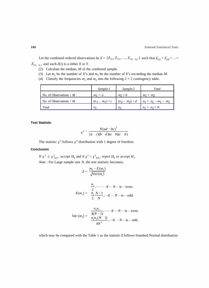
180 Selected Statistical Tests
Let the combined ordered observations be Z = },,,{ )21()2()1( nnZZZ +… such that Z(1) < Z(2) < …<
)( 21 nnZ + and each Z(i) is a either X or Y.(2) Calculate the median, M of the combined sample.(3) Let m1 be the number of X’s and m2 be the number of Y’s exceeding the median M.(4) Classify the frequencies m1 and m2 into the following 2 × 2 contingency table.
Test Statistic
χ2 =))()()((
)( 2
dcbadbcabcadN
++++−
The statistic χ2 follows χ2 distribution with 1 degree of freedom.
Conclusion
If χ2 ≤ χ2(α) , accept H0 and if χ2 > χ2
(α) , reject H0 or accept H1.
Note : For Large sample size N, the test statistic becomes,
Z =)(
)(
1
11
mVar
mEm −
E(m1) =
−.oddisif,
12
.evenisif,21
1
LLLL
LLLLLL
NN
Nn
Nn
Var (m1) =
+−
.oddisif,4
)1(
.evenisif,)1(4
221
21
LLLL
LLLLL
NN
Nnn
NN
nn
which may be compared with the Table 1 as the statistic Z follows Standard Normal distribution.
Sample-1 Sample-2 Total
No. of Observations > M m1 = a m2 = b m1 + m2
No. of Observations < M (n1 – m1) = c (n2 – m2) = d n1 + n2 – m1 – m2
Total n1 n2 n1 + n2 = N
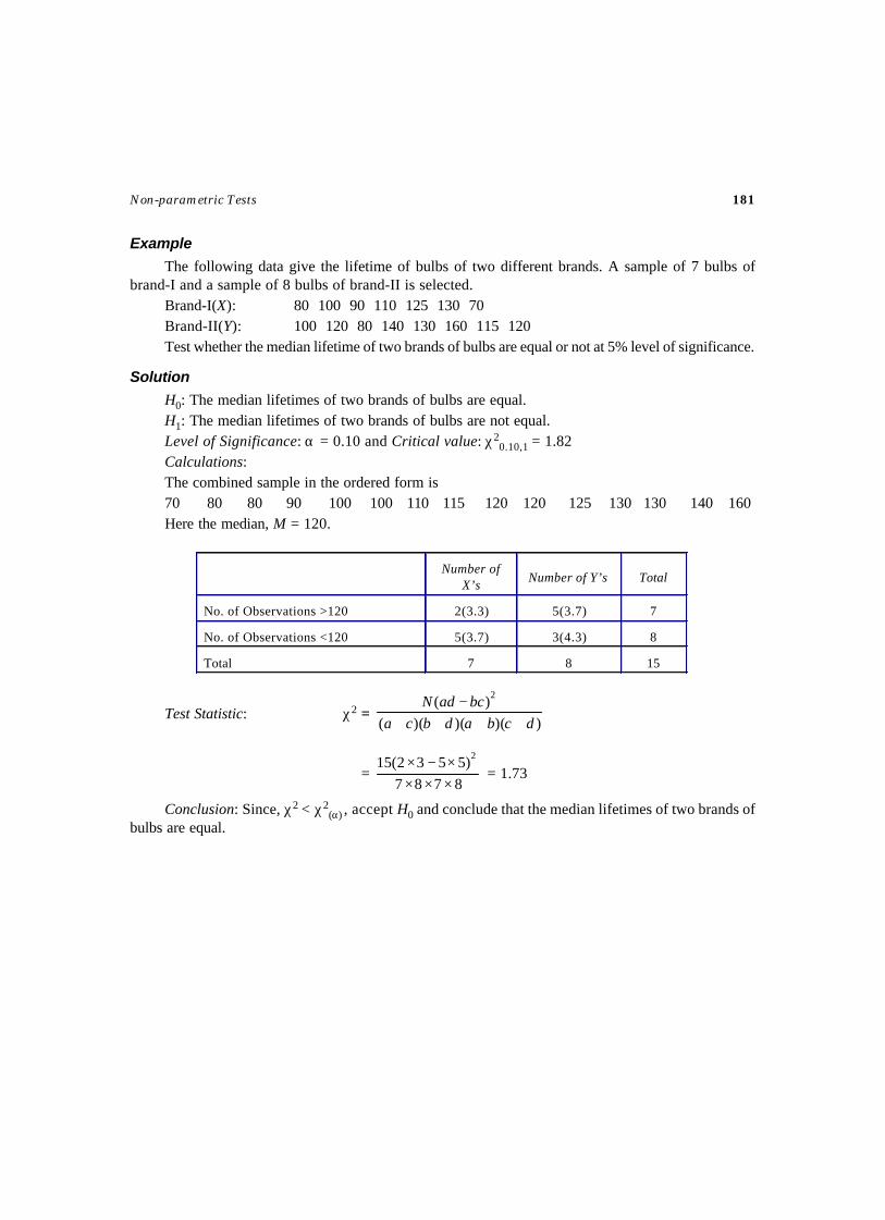
Non-parametric Tests 181
Example
The following data give the lifetime of bulbs of two different brands. A sample of 7 bulbs ofbrand-I and a sample of 8 bulbs of brand-II is selected.
Brand-I(X): 80 100 90 110 125 130 70Brand-II(Y): 100 120 80 140 130 160 115 120Test whether the median lifetime of two brands of bulbs are equal or not at 5% level of significance.
Solution
H0: The median lifetimes of two brands of bulbs are equal.H1: The median lifetimes of two brands of bulbs are not equal.Level of Significance: α = 0.10 and Critical value: χ2
0.10,1 = 1.82Calculations:The combined sample in the ordered form is70 80 80 90 100 100 110 115 120 120 125 130 130 140 160Here the median, M = 120.
Test Statistic: χ2 =))()()((
)( 2
dcbadbcabcadN
++++−
=8787
)5532(15 2
××××−×
= 1.73
Conclusion: Since, χ2 < χ2(α) , accept H0 and conclude that the median lifetimes of two brands of
bulbs are equal.
Number of X’s
Number of Y’s Total
No. of Observations >120 2(3.3) 5(3.7) 7
No. of Observations <120 5(3.7) 3(4.3) 8
Total 7 8 15
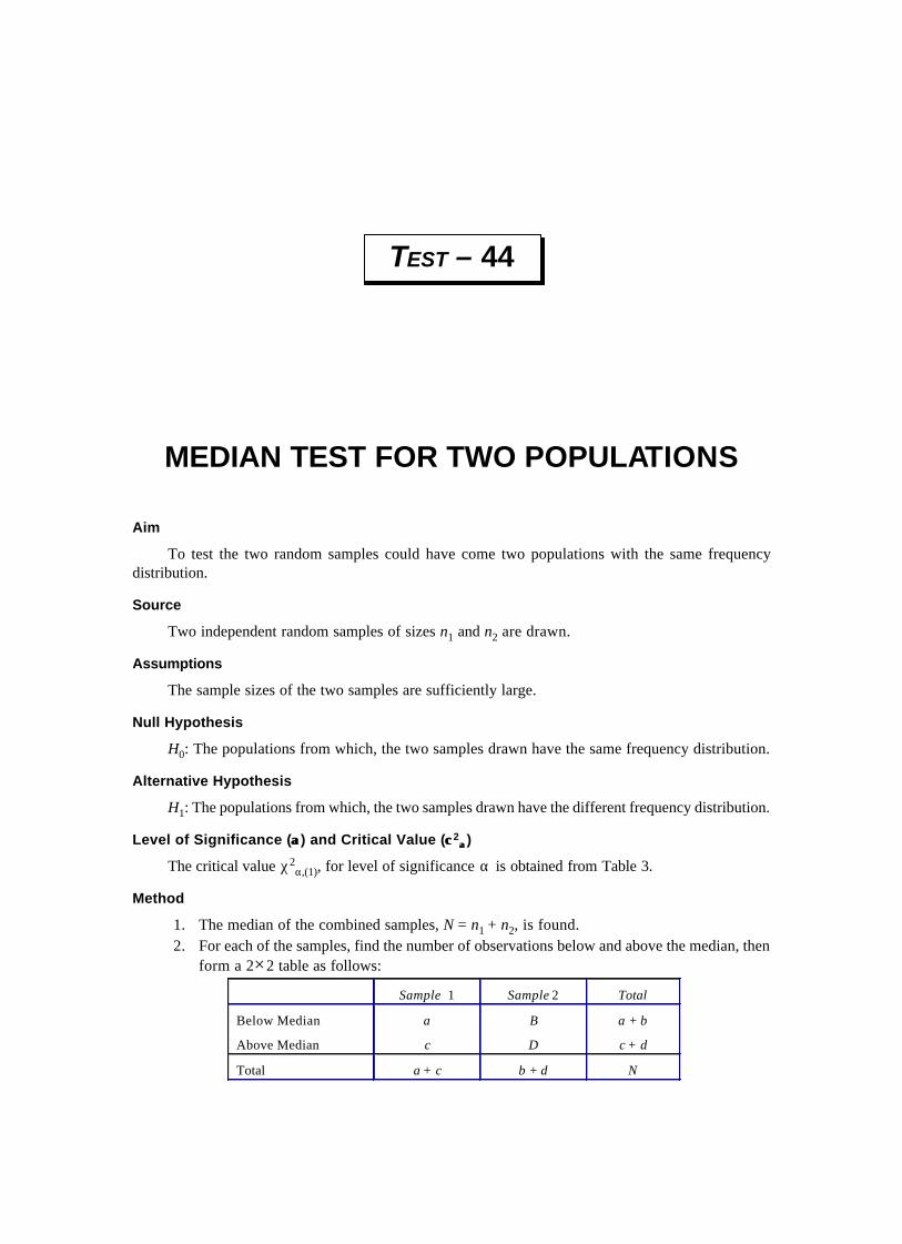
Aim
To test the two random samples could have come two populations with the same frequencydistribution.
Source
Two independent random samples of sizes n1 and n2 are drawn.
Assumptions
The sample sizes of the two samples are sufficiently large.
Null Hypothesis
H0: The populations from which, the two samples drawn have the same frequency distribution.
Alternative Hypothesis
H1: The populations from which, the two samples drawn have the different frequency distribution.
Level of Significance (αα) and Critical Value (χχ2αα )
The critical value χ2α,(1), for level of significance α is obtained from Table 3.
Method
1. The median of the combined samples, N = n1 + n2, is found.2. For each of the samples, find the number of observations below and above the median, then
form a 2×2 table as follows:
MEDIAN TEST FOR TWO POPULATIONS
TEST – 44
Sample 1 Sample 2 Total
Below Median
Above Median
a
c
B
D
a + b
c + d
Total a + c b + d N
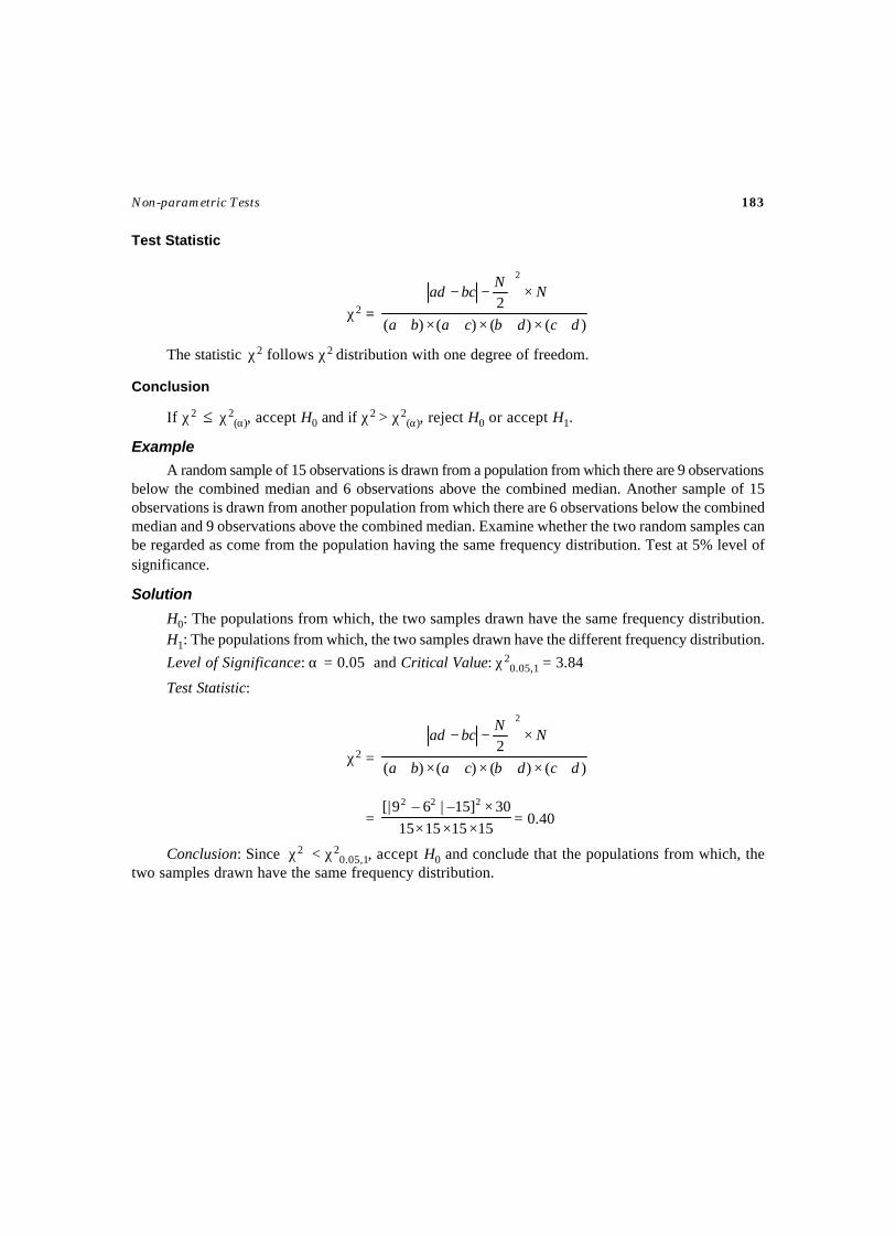
Non-parametric Tests 183
Test Statistic
χ2 =)()()()(
2
2
dcdbcaba
NN
bcad
+×+×+×+
×
−−
The statistic χ2 follows χ2 distribution with one degree of freedom.
Conclusion
If χ2 ≤ χ2(α), accept H0 and if χ2 > χ2
(α), reject H0 or accept H1.
Example
A random sample of 15 observations is drawn from a population from which there are 9 observationsbelow the combined median and 6 observations above the combined median. Another sample of 15observations is drawn from another population from which there are 6 observations below the combinedmedian and 9 observations above the combined median. Examine whether the two random samples canbe regarded as come from the population having the same frequency distribution. Test at 5% level ofsignificance.
Solution
H0: The populations from which, the two samples drawn have the same frequency distribution.H1: The populations from which, the two samples drawn have the different frequency distribution.
Level of Significance: α = 0.05 and Critical Value: χ20.05,1 = 3.84
Test Statistic:
χ2 =)()()()(
2
2
dcdbcaba
NN
bcad
+×+×+×+
×
−−
=15151515
30]15–|6–9[| 222
××××
= 0.40
Conclusion: Since χ2 < χ20.05,1, accept H0 and conclude that the populations from which, the
two samples drawn have the same frequency distribution.
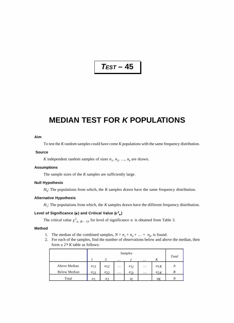
Aim
To test the K random samples could have come K populations with the same frequency distribution.
Source
K independent random samples of sizes n1, n2, …, nk are drawn.
Assumptions
The sample sizes of the K samples are sufficiently large.
Null Hypothesis
H0: The populations from which, the K samples drawn have the same frequency distribution.
Alternative Hypothesis
H1: The populations from which, the K samples drawn have the different frequency distribution.
Level of Significance (αα) and Critical Value (χχ2αα )
The critical value χ2α, (K – 1), for level of significance α is obtained from Table 3.
Method
1. The median of the combined samples, N = n1 + n2 + … + nk, is found.2. For each of the samples, find the number of observations below and above the median, then
form a 2×K table as follows:
MEDIAN TEST FOR K POPULATIONS
TEST – 45
Samples
1 2 … j … K Total
Above Median
Below Median
a11
a21
a12
a22
…
…
a1j
a2j
…
…
a1K
a2K
A
B
Total a1 a2 aj aK N
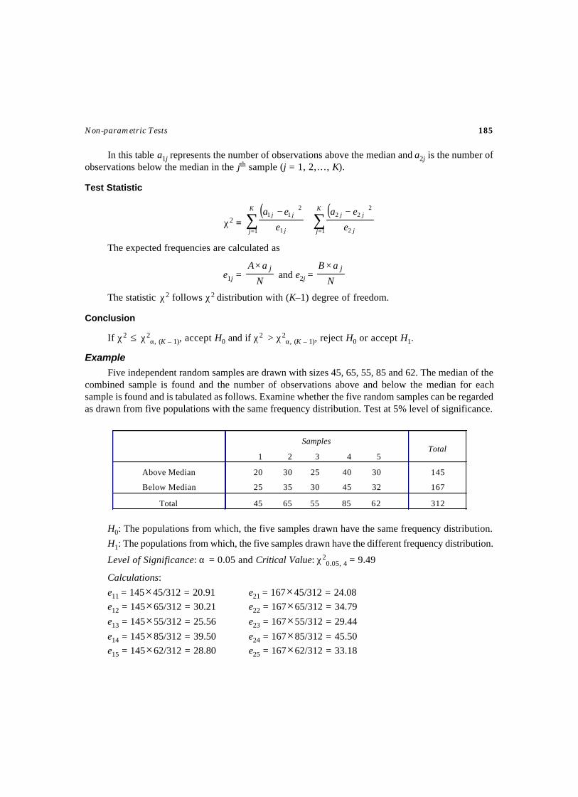
Non-parametric Tests 185
In this table a1j represents the number of observations above the median and a2j is the number ofobservations below the median in the jth sample (j = 1, 2,…, K).
Test Statistic
χ2 =( ) ( )
∑∑==
−+
− K
j j
jjK
j j
jj
e
ea
e
ea
1 2
222
1 1
211
The expected frequencies are calculated as
e1j =N
aA j× and e2j = N
aB j×
The statistic χ2 follows χ2 distribution with (K–1) degree of freedom.
Conclusion
If χ2 ≤ χ2α, (K – 1), accept H0 and if χ2 > χ2
α, (K – 1), reject H0 or accept H1.
Example
Five independent random samples are drawn with sizes 45, 65, 55, 85 and 62. The median of thecombined sample is found and the number of observations above and below the median for eachsample is found and is tabulated as follows. Examine whether the five random samples can be regardedas drawn from five populations with the same frequency distribution. Test at 5% level of significance.
H0: The populations from which, the five samples drawn have the same frequency distribution.
H1: The populations from which, the five samples drawn have the different frequency distribution.
Level of Significance: α = 0.05 and Critical Value: χ20.05, 4 = 9.49
Calculations:
e11 = 145×45/312 = 20.91 e21 = 167×45/312 = 24.08e12 = 145×65/312 = 30.21 e22 = 167×65/312 = 34.79
e13 = 145×55/312 = 25.56 e23 = 167×55/312 = 29.44
e14 = 145×85/312 = 39.50 e24 = 167×85/312 = 45.50e15 = 145×62/312 = 28.80 e25 = 167×62/312 = 33.18
Samples
1 2 3 4 5 Total
Above Median
Below Median
20 30 25 40 30
25 35 30 45 32
145
167
Total 45 65 55 85 62 312
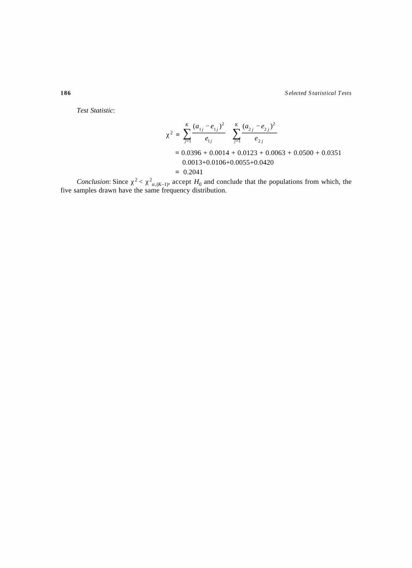
186 Selected Statistical Tests
Test Statistic:
χ2 = ∑∑==
−+
− K
j j
jjK
j j
jj
e
ea
e
ea
1 2
222
1 1
211 )()(
= 0.0396 + 0.0014 + 0.0123 + 0.0063 + 0.0500 + 0.03510.0013+0.0106+0.0055+0.0420
= 0.2041Conclusion: Since χ2 < χ2
α,(K–1), accept H0 and conclude that the populations from which, thefive samples drawn have the same frequency distribution.

WALD–WOLFOWITZ RUN TEST
TEST – 46
Aim
To test the two samples have been drawn from the populations having the same density functions.
Definition (RUN)
A run is defined as a sequence of letters of one type surrounded by a sequence of letters of theother type, and the number of elements in a run is referred to as the length of the run.
Source
A random sample of n1 observations, arranged in order of magnitude as, X1, X2,…, Xn1 drawnfrom a population with density function f1(.) and a random sample of n2 observations, arranged inorder of magnitude as, Y1, Y2,…, Yn2 drawn from another population with density function f2(.)
Assumption
The two samples are drawn independently.
Null Hypothesis
H0: The populations from which the two samples drawn have the same density function. i.e.,H0: f1(.) = f2(.).
Alternative Hypothesis
H1: f1(.) ≠ f2(.).
Level of Significance (αα) and Critical Value (Uαα )
The Critical value, Uα for the level of significance, α and for sample sizes, n1 and n2 is obtainedfrom Table 7.
Method
1. Combine the two samples and arrange the observations in order of magnitude, say, X1 X2 Y1X3 Y2 Y3 X4 Y4 X5 … such that X1 <X2 <Y1 <X3 <Y2 <Y3 <X4 <Y4 <X5 … Let the combined
188 Selected Statistical Tests
ordered observations be Z = {Z(1) , Z(2) , …Z(n1 + n2)} such that Z(1) < Z(2) < …< Z(n1+n2) andeach Z(i) is a either X or Y. Replace each X by a ‘0’ and each Y by a ‘1’, one gets a sequenceof n1 0’s and n2 1’s in Z.
2. Let r1 be the number of runs of 0’s and r2 be the number of runs of 1’s.
Test StatisticU = r1 + r2
Conclusion
If U ≥ Uα accept H0 and if U < Uα reject H0 or accept H1.
Note
For sufficiently large n1 and n2, (i.e., n1 > 10, n2 > 10), the statistic becomes,
Z = )(
)(
UVar
UEU −
E(U) = 12
21
21 ++ nnnn
Var (U) = )1()(
)2(2
212
21
212121
−++
−−
nnnn
nnnnnn
which may be compared with the Table 1 as the statistic Z follows Standard Normal distribution.
Example
A random sample of 8 households is selected from a village, A whose daily expense on milk as 1115 17 19 25 27 31 33. Another sample of 9 households is selected from village B whose expense onmilk is 12 16 20 22 28 30 36 38 42. Test whether the households of the two villages are same onspending daily milk expenses.
Solution
H0: The households of the two villages are same on spending daily milk expenses.H1: The households of the two villages are not same on spending daily milk expenses.
Level of Significance: α = 0.05 and Critical value: U0.05, (8, 9) = 5.
Calculations:The pooled ordered observation is11 12 15 16 17 19 20 22 25 27 28 30 31 33 36 38 42The representation of ‘0’ for X’s and ‘1’ for Y’s is0 1 0 1 0 0 1 1 0 0 1 1 0 0 1 1 1Here 0 and 1 have 5 runs each. i.e., r1 = 5 and r2 = 5.Test Statistic: U = r1 + r2 = 10.Conclusion: Since U > U0.05, (8, 9), H0 is accepted and concluded that the households of the two
villages are same on spending daily milk expenses.
Aim
To test the K random samples drawn from the K populations have the same mean.
Source
K random samples, each with sizes ni, (i = 1, 2, …, K) be drawn independently from K populations.Let n1 + n2 + … + nK = N.
Assumptions
(i) The sample sizes of each sample should be at least 5.(ii) The sample sizes need not be equal.
(iii) The frequency distributions of K populations should be continuous.
Null Hypothesis
H0: The means of the K populations are equal.
Alternative Hypothesis
H1: The means of the K populations are not equal.
Level of Significance (αα) and Critical Value (χχ2αα )
The critical value χ2α,(K–1), for level of significance α is obtained from Table 3.
Method
1. Combine all the K samples and arrange the observations in increasing order of magnitude.2. Assign ranks to the combined observations Z. If the observations are equal, the mean of the
available rank numbers is assigned.3. Find the rank sum of each of the K samples in the combined ordered sample.4. Let Ri be the rank sum of the ith sample.
KRUSKALL–WALLIS RANK SUM TEST (H TEST)
TEST – 47
190 Selected Statistical Tests
Test Statistic
H =
Σ+ i
i
nR
NN
2
)1(12
– 3 (N + 1)
The statistic H follows χ2 distribution with (K–1) degrees of freedom.
Conclusion
If H ≤ χ2(α), accept H0 and if H > χ2
(α), reject H0 or accept H1.
Example
The following table shows three independent samples of sizes 9, 6 and 5 drawn from threepopulations of children whose weight and their ranks. Test whether the mean weight of the childrenfrom the three populations is same at 5% level of significance.
Solution
H0: The mean weight of the children from the three populations is same.H1: The mean weight of the children from the three populations is not same.
Level of Significance: α = 0.10 and Critical Value: 22χ = 4.61
Calculations:n1 = 9; n2 = 6; n3 = 5; N = 20;R1 = 76.5 R2 = 74 R3 = 55.5Test Statistic:
H =
Σ+ i
i
nR
NN
2
)1(12
– 3(N + 1)
= 2135
5.55674
95.76
212012 2
×−
++×× = 2.15
Conclusion: Since, H < χ2(α), H0 is accepted and concluded that the mean weight of the children
from the three populations is same.
1 11.7
1
1 11.9
2
1 16.1
3
1 17.5
4
1 20.5
7
1 25.1
10.5
1 30.5
14
1 32.1
15
1 82.5
20
2 19.6
6
2 21.8
8
2 25.2
12
2 33.2
16.5
2 33.2
16.5
2 34.1
19
3 18.4
5
3 22.9
9
3 25.1
10.5
3 29.7
13
3 33.5
18
SampleValueRank
SampleValueRank
Aim
To test the two random samples be drawn from the populations having the same mean, based onthe rank sum of the sample.
Source
A random sample of n1 observations, arranged in order of magnitude as, X1, X2, …, Xn1 drawnfrom a population with density function f1(.) and a random sample of n2 observations, arranged inorder of magnitude as, Y1, Y2, …, Yn2 drawn from another population with density function f2(.).
Assumptions
(i) The two samples drawn are independent.(ii) The populations have continuous frequency distributions.
Null Hypothesis
H0: The populations from which the samples drawn have the same mean.
Alternative Hypothesis
H1: The populations, from which, the samples drawn have different mean.
Level of Significance (αα) and Critical Value (R αα )
The critical value, Rα for the level of significance α , and for sample sizes, n1 and n2 is obtainedfrom Table 8.
Method
1. Combine the two samples and arrange the observations in order of magnitude, say, X1 X2 Y1X3 Y2 Y3 X4 Y4 X5 … such that X1 <X2 <Y1 <X3 <Y2 <Y3 <X4 <Y4 <X5 … Let the combinedordered observations be Z = {Z(1) , Z(2) , …Z(n1 + n2)} such that Z(1) < Z(2) < …< Z(n1 + n2) andeach Z(i) is a either X or Y.
MANN–WHITNEY–WILCOXON RANK SUMTEST
TEST – 48
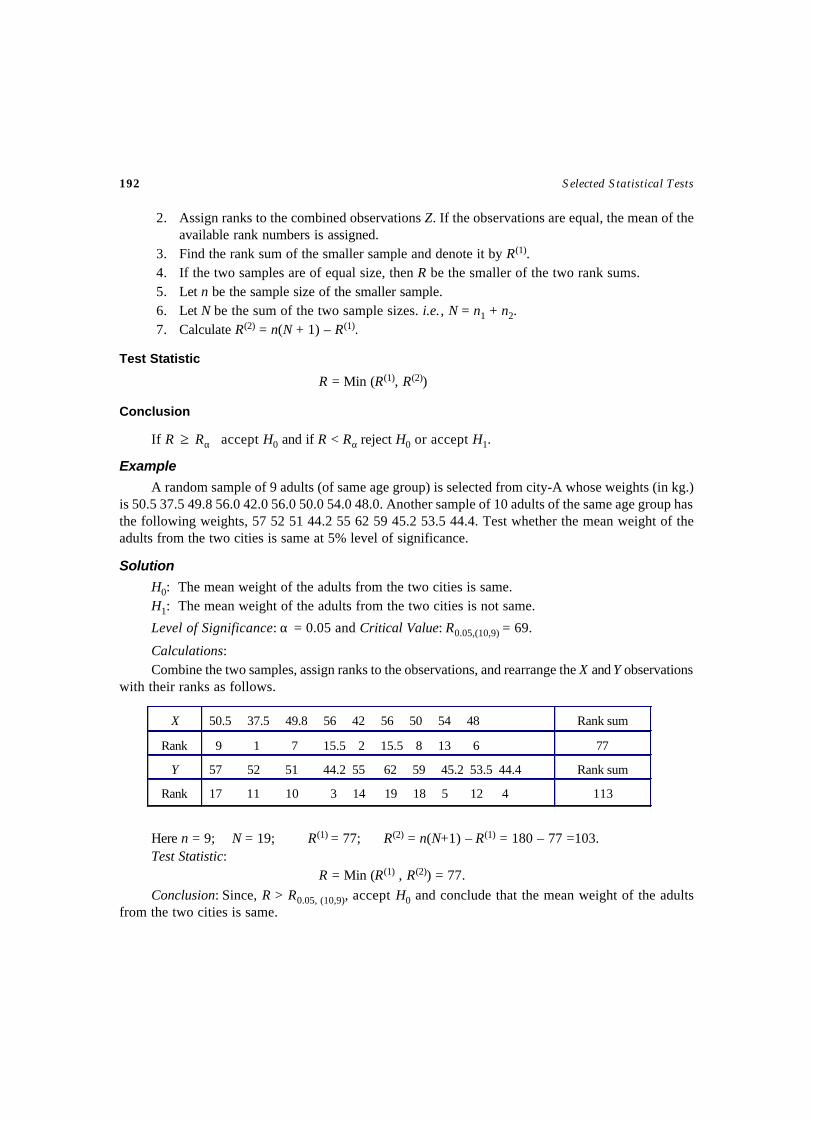
192 Selected Statistical Tests
2. Assign ranks to the combined observations Z. If the observations are equal, the mean of theavailable rank numbers is assigned.
3. Find the rank sum of the smaller sample and denote it by R(1).4. If the two samples are of equal size, then R be the smaller of the two rank sums.5. Let n be the sample size of the smaller sample.6. Let N be the sum of the two sample sizes. i.e., N = n1 + n2.7. Calculate R(2) = n(N + 1) – R(1).
Test Statistic
R = Min (R(1), R(2))
Conclusion
If R ≥ Rα accept H0 and if R < Rα reject H0 or accept H1.
Example
A random sample of 9 adults (of same age group) is selected from city-A whose weights (in kg.)is 50.5 37.5 49.8 56.0 42.0 56.0 50.0 54.0 48.0. Another sample of 10 adults of the same age group hasthe following weights, 57 52 51 44.2 55 62 59 45.2 53.5 44.4. Test whether the mean weight of theadults from the two cities is same at 5% level of significance.
Solution
H0: The mean weight of the adults from the two cities is same.H1: The mean weight of the adults from the two cities is not same.
Level of Significance: α = 0.05 and Critical Value: R0.05,(10,9) = 69.
Calculations:Combine the two samples, assign ranks to the observations, and rearrange the X and Y observations
with their ranks as follows.
Here n = 9; N = 19; R(1) = 77; R(2) = n(N+1) – R(1) = 180 – 77 =103.Test Statistic:
R = Min (R(1) , R(2)) = 77.Conclusion: Since, R > R0.05, (10,9), accept H0 and conclude that the mean weight of the adults
from the two cities is same.
X 50.5 37.5 49.8 56 42 56 50 54 48 Rank sum
Rank 9 1 7 15.5 2 15.5 8 13 6 77
Y 57 52 51 44.2 55 62 59 45.2 53.5 44.4 Rank sum
Rank 17 11 10 3 14 19 18 5 12 4 113
Aim
To test that the two random samples are drawn from the populations having the same densityfunctions.
Source
A random sample of n1 observations, arranged in order of magnitude as, X1, X2,…, 1nX drawn
from a population with density function f1(.) and a random sample of n2 observations, arranged in
order of magnitude as, Y1, Y2,…, 2nY drawn from another population with density function f2(.).
Assumptions
(i) The two samples drawn are independent.(ii) The populations have continuous frequency distributions.
(iii) The sample sizes should be sufficiently large.
Null Hypothesis
H0: The populations, from which, the two samples drawn have the same density function. i.e.,H0: f1(.) = f2(.).
Alternative Hypothesis
H1: f1(.) ≠ f2(.).
Level of Significance (αα) and Critical Value (Z αα )
The critical value, Zα for the level of significance, α is obtained from Table 1.
Method
1. Combine the two samples and arrange the observations in order of magnitude, say, X1 X2 Y1X3 Y2 Y3 X4 Y4 X5 … such that X1 <X2 <Y1 <X3 <Y2 <Y3 <X4 <Y4 <X5 … Let the combined
MANN–WHITNEY–WILCOXON U-TEST
TEST – 49
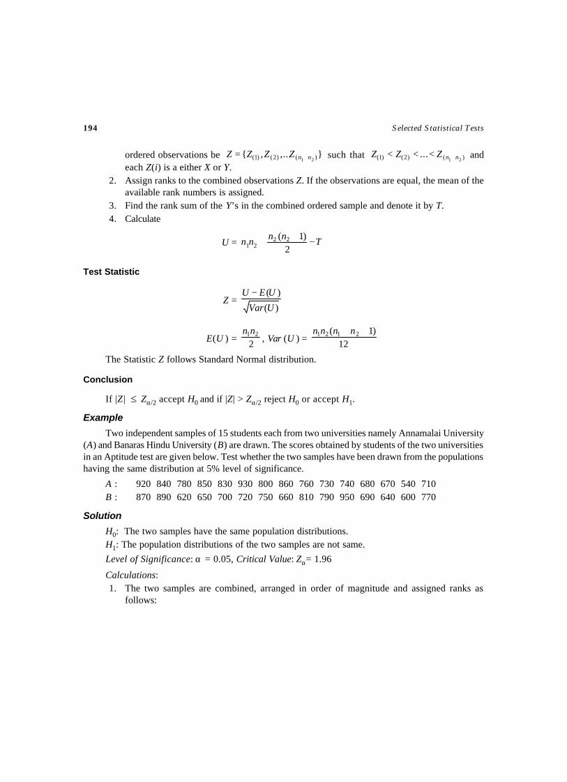
194 Selected Statistical Tests
ordered observations be },...,{ )()2()1( 21 nnZZZZ += such that )()2()1( 21... nnZZZ +<<< and
each Z(i) is a either X or Y.2. Assign ranks to the combined observations Z. If the observations are equal, the mean of the
available rank numbers is assigned.3. Find the rank sum of the Y’s in the combined ordered sample and denote it by T.4. Calculate
U = Tnnnn −++2
)1( 2221
Test Statistic
Z =)(
)(
UVar
UEU −
E(U ) = 221nn
, Var (U ) = 12)1( 2121 ++ nnnn
The Statistic Z follows Standard Normal distribution.
Conclusion
If |Z| ≤ Zα/2 accept H0 and if |Z| > Zα/2 reject H0 or accept H1.
Example
Two independent samples of 15 students each from two universities namely Annamalai University(A) and Banaras Hindu University (B) are drawn. The scores obtained by students of the two universitiesin an Aptitude test are given below. Test whether the two samples have been drawn from the populationshaving the same distribution at 5% level of significance.
A : 920 840 780 850 830 930 800 860 760 730 740 680 670 540 710B : 870 890 620 650 700 720 750 660 810 790 950 690 640 600 770
Solution
H0: The two samples have the same population distributions.H1: The population distributions of the two samples are not same.
Level of Significance: α = 0.05, Critical Value: Zα= 1.96
Calculations:1. The two samples are combined, arranged in order of magnitude and assigned ranks as
follows:
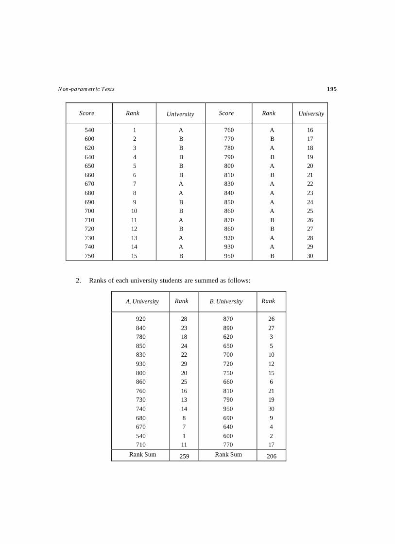
Non-parametric Tests 195
2. Ranks of each university students are summed as follows:
540 600
620
640 650
660 670
680
690 700
710 720
730 740
750
1 2
3
4 5
6 7
8
9 10
11 12
13 14
15
A B
B
B B
B A
A
B B
A B
A A
B
760 770
780
790 800
810 830
840
850 860
870 860
920 930
950
A B
A
B A
B A
A
A A
B B
A A
B
16 17
18
19 20
21 22
23
24 25
26 27
28 29
30
Score Rank University Score Rank University
920
840 780
850 830
930
800 860
760 730
740
680 670
540 710
28
23 18
24 22
29
20 25
16 13
14
8 7
1 11
870
890 620
650 700
720
750 660
810 790
950
690 640
600 770
26
27 3
5 10
12
15 6
21 19
30
9 4
2 17
259 206
A. University B. UniversityRank Rank
Rank Sum Rank Sum
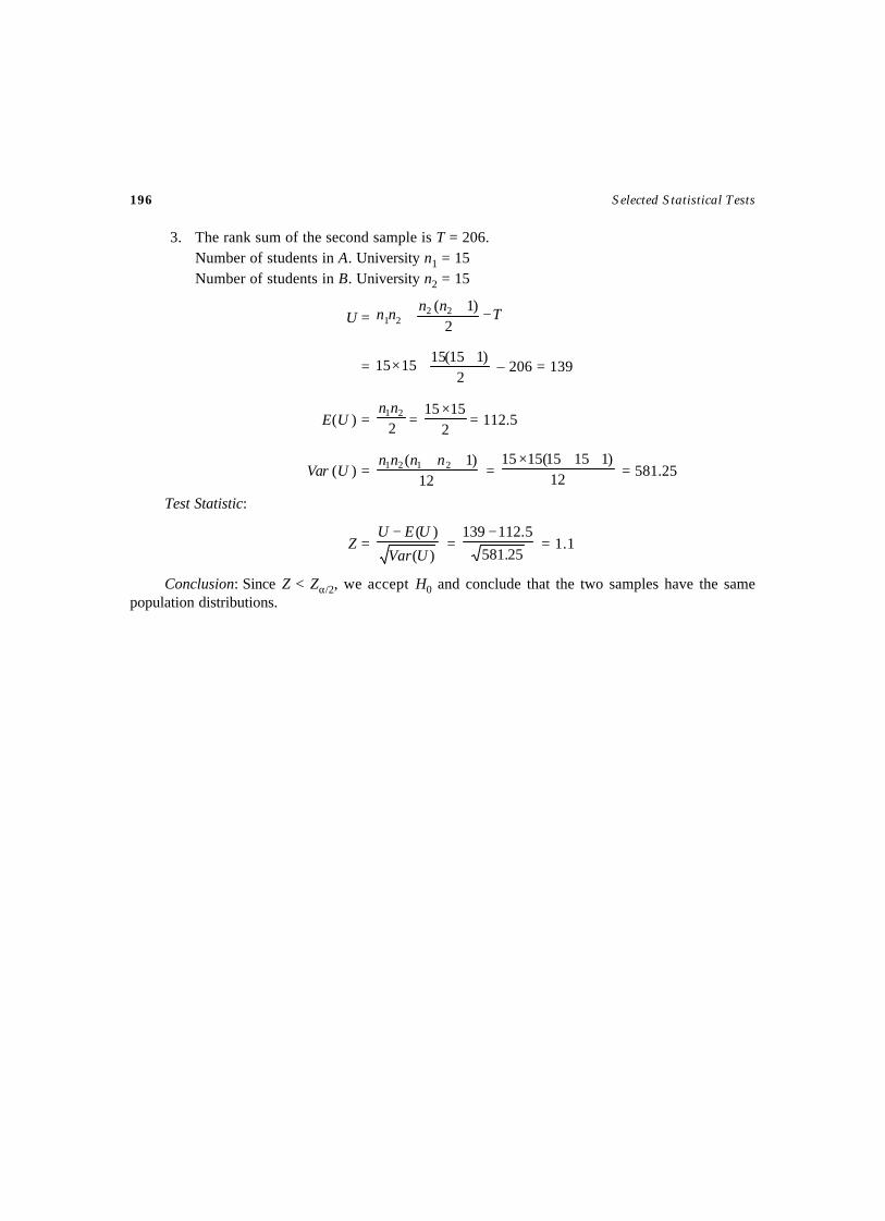
196 Selected Statistical Tests
3. The rank sum of the second sample is T = 206.Number of students in A. University n1 = 15Number of students in B. University n2 = 15
U = Tnnnn −++2
)1( 2221
=2
)115(151515 ++× – 206 = 139
E(U ) = 221nn
= 2
1515 ×= 112.5
Var (U ) =12
)1( 2121 ++ nnnn = 12
)11515(1515 ++× = 581.25
Test Statistic:
Z =)(
)(
UVar
UEU − =
25.581
5.112139 − = 1.1
Conclusion: Since Z < Zα/2, we accept H0 and conclude that the two samples have the samepopulation distributions.

Aim
To test the population distribution F(x) be regarded as F0(x), based on a random sample.
Source
Let Xi, (i = 1, 2, …, n) a random sample of n observations be drawn from a population. Let F0(x)be the cumulative distribution of a specified (given) population.
Null Hypothesis
H0: The population distribution F(x) is F0(x).
Alternative Hypothesis
H1: The population distribution F(x) is not F0(x).
Level of Significance (αα) and Critical Value (D αα )
The critical value Dα for the level of significance, α and for the sample size, n is obtained fromthe Table 9.
Method
1. Calculate the cumulative distribution F0(x) based on the sample observations and the specified(given) population distribution.
2. Obtain the cumulative distribution of the sample, Fn(x) be the empirical distribution function
defined as a step function, Fn(x) = (Number of observations Xi ≤ x)/n.3. Find the absolute difference |F0(x) – Fn(x)|
Test Statistic
D = Max |F0(x) – Fn(x)|
KOLMOGOROV–SMIRNOV TEST FORGOODNESS OF FIT
TEST – 50
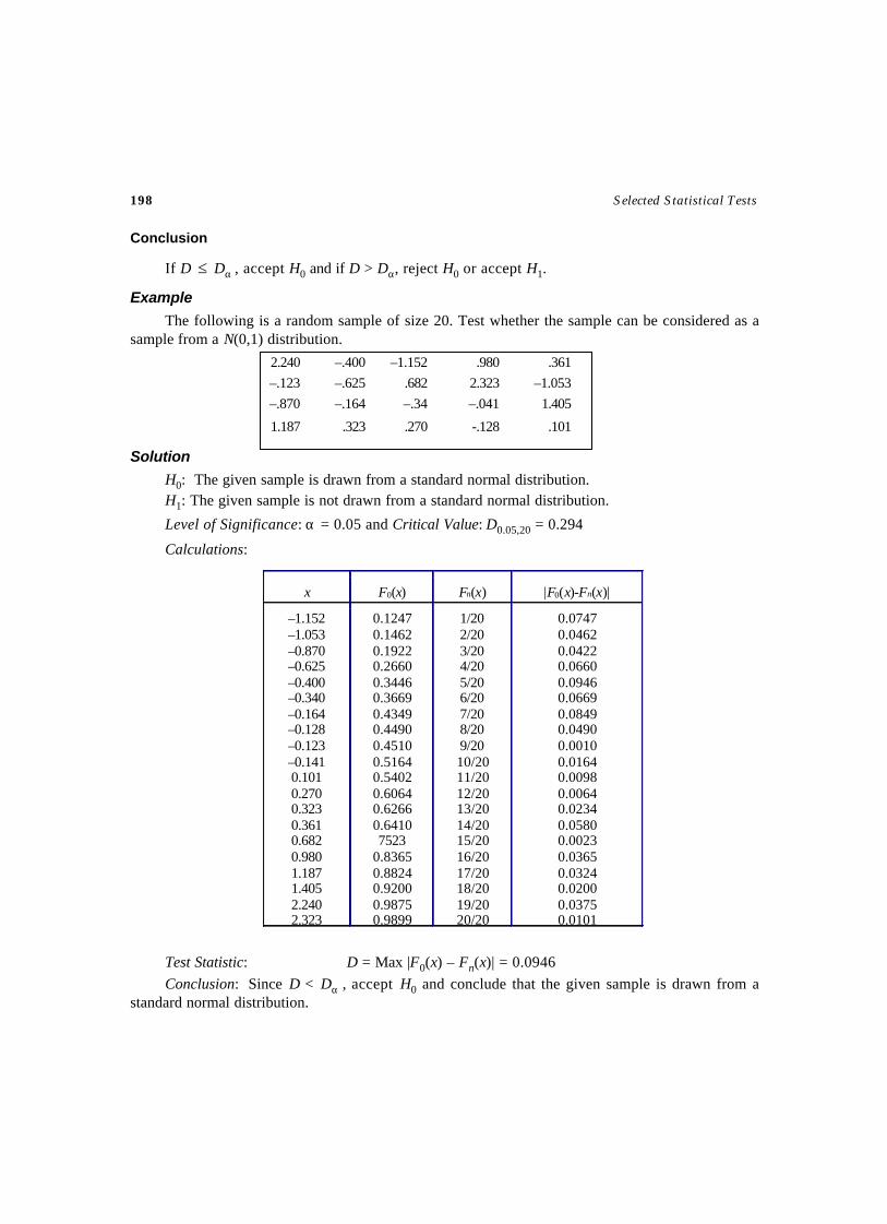
198 Selected Statistical Tests
Conclusion
If D ≤ Dα , accept H0 and if D > Dα, reject H0 or accept H1.
Example
The following is a random sample of size 20. Test whether the sample can be considered as asample from a N(0,1) distribution.
2.240 –.400 –1.152 .980 .361
–.123 –.625 .682 2.323 –1.053
–.870 –.164 –.34 –.041 1.405
1.187 .323 .270 -.128 .101
Solution
H0: The given sample is drawn from a standard normal distribution.H1: The given sample is not drawn from a standard normal distribution.
Level of Significance: α = 0.05 and Critical Value: D0.05,20 = 0.294
Calculations:
Test Statistic: D = Max |F0(x) – Fn(x)| = 0.0946Conclusion: Since D < Dα , accept H0 and conclude that the given sample is drawn from a
standard normal distribution.
x F0(x) Fn(x) |F0(x)-Fn(x)|
–1.152 –1.053 –0.870 –0.625 –0.400 –0.340 –0.164 –0.128 –0.123 –0.141 0.101 0.270 0.323 0.361 0.682 0.980 1.187 1.405 2.240 2.323
0.1247 0.1462 0.1922 0.2660 0.3446 0.3669 0.4349 0.4490 0.4510 0.5164 0.5402 0.6064 0.6266 0.6410 7523
0.8365 0.8824 0.9200 0.9875 0.9899
1/20 2/20 3/20 4/20 5/20 6/20 7/20 8/20 9/20 10/20 11/20 12/20 13/20 14/20 15/20 16/20 17/20 18/20 19/20 20/20
0.0747 0.0462 0.0422 0.0660 0.0946 0.0669 0.0849 0.0490 0.0010 0.0164 0.0098 0.0064 0.0234 0.0580 0.0023 0.0365 0.0324 0.0200 0.0375 0.0101
Aim
To test the two population distributions are identical, based on the two sample distributions.
Source
Let Xi, (i = 1, 2,…, n) be a random sample of n observations be drawn from a population. Let Yi,(i = 1, 2,…, n) be a random sample of n observations be drawn from another population.
Null Hypothesis
H0: The two population distributions are identical. i.e., There is no significant difference betweenthe two sample distributions.
Alternative Hypothesis
H1: The two population distributions are not identical. i.e., there is a significant difference betweenthe two sample distributions.
Level of Significance (αα) and Critical Value (D αα )
The critical value Dα for the level of significance, α and for the sample size, n is obtained fromthe Table 9.
Method
1. Calculate the cumulative frequencies for each of the observations, Xi and denote it by C(x),and for each of the observations, Yi and denote it by C(y).
2. Obtain the cumulative distribution of the two samples, Fn(x) and Fn(y) are the empirical
distribution functions defined as a step function, Fn(x) = (Number of observations (Xi ≤ x)/
n and Fn(y) = (Number of observations Yi ≤ y)/n.3. Find the absolute difference |Fn(x) – Fn(y)|
KOLMOGOROV–SMIRNOV TEST FORCOMPARING TWO POPULATIONS
TEST – 51
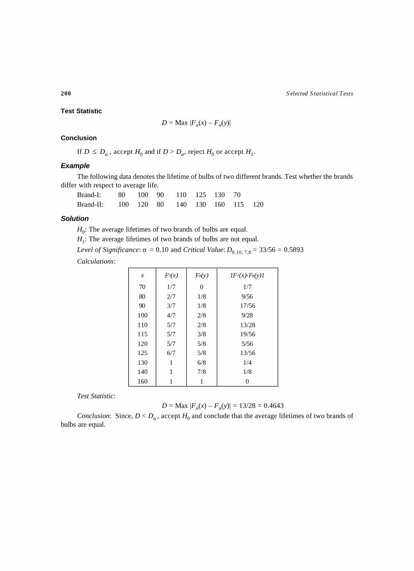
200 Selected Statistical Tests
Test Statistic
D = Max |Fn(x) – Fn(y)|
Conclusion
If D ≤ Dα , accept H0 and if D > Dα, reject H0 or accept H1.
Example
The following data denotes the lifetime of bulbs of two different brands. Test whether the brandsdiffer with respect to average life.
Brand-I: 80 100 90 110 125 130 70Brand-II: 100 120 80 140 130 160 115 120
Solution
H0: The average lifetimes of two brands of bulbs are equal.H1: The average lifetimes of two brands of bulbs are not equal.
Level of Significance: α = 0.10 and Critical Value: D0.10, 7,8 = 33/56 = 0.5893
Calculations:
Test Statistic:D = Max |Fn(x) – Fn(y)| = 13/28 = 0.4643
Conclusion: Since, D < Dα , accept H0 and conclude that the average lifetimes of two brands ofbulbs are equal.
x F7(x) F8(y) 1F7(x)-F8(y)1
70
80 90
100
110 115
120 125
130 140
160
1/7
2/7 3/7
4/7
5/7 5/7
5/7 6/7
1 1
1
0
1/8 1/8
2/8
2/8 3/8
5/8 5/8
6/8 7/8
1
1/7
9/56 17/56
9/28
13/28 19/56
5/56 13/56
1/4 1/8
0
Aim
To test the existence of correlation between the two pairs of observations in the population basedon a sample.
Source
Let (Xi, Yi), i = 1, 2, …, n be a random sample of n pairs of observations drawn.
Assumptions
(i) The population distribution is continuous.(ii) The observations should be obtained in pairs.
Null Hypothesis
H0: There exists correlation between the pairs (X, Y)
Alternative Hypothesis
H1: There exists correlation between the pairs (X, Y)
Level of Significance (αα) and Critical Value (R αα )
The critical value Rα for the level of significance, α and for the sample size, n is obtained from theTable 10.
Method
1. Assign ranks to each of the observations Xi and Yi independently and denote them by r (Xi)and r (Yi) respectively.
2. For each pair of observations, find the difference of the ranks di = r(Xi) – r( Yi) ,i = 1, 2, …, n.
3. Calculate r = ∑=
n
iid
1
2
SPEARMAN RANK CORRELATION TEST
TEST – 52
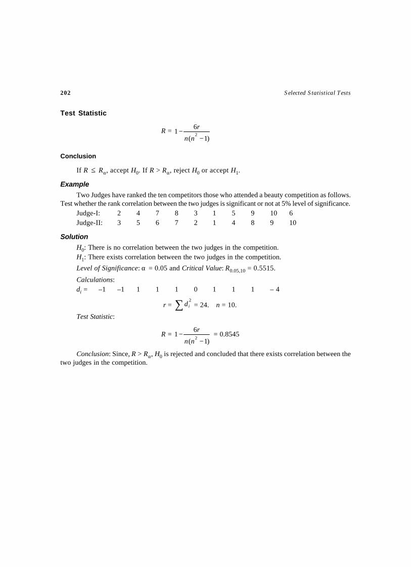
202 Selected Statistical Tests
Test Statistic
R =)1(
61 2
−−
nn
r
Conclusion
If R ≤ Rα, accept H0. If R > Rα, reject H0 or accept H1.
Example
Two Judges have ranked the ten competitors those who attended a beauty competition as follows.Test whether the rank correlation between the two judges is significant or not at 5% level of significance.
Judge-I: 2 4 7 8 3 1 5 9 10 6Judge-II: 3 5 6 7 2 1 4 8 9 10
Solution
H0: There is no correlation between the two judges in the competition.H1: There exists correlation between the two judges in the competition.
Level of Significance: α = 0.05 and Critical Value: R0.05,10 = 0.5515.
Calculations:di = –1 –1 1 1 1 0 1 1 1 – 4
r = ∑ 2id = 24. n = 10.
Test Statistic:
R =)1(
61
2 −−
nn
r = 0.8545
Conclusion: Since, R > Rα, H0 is rejected and concluded that there exists correlation between thetwo judges in the competition.
Aim
To test the order of observations in a sample is random, obtained from any experiment.
Source
A sample of n observations is drawn from any experiment.
Assumptions
(i) The sample observations be obtained under similar conditions.(ii) Retain the observations in the order in which they occur. That is, Xi is the ith observation in
the outcome of an experiment.
Null Hypothesis
H0: The sample observations obtained is random.
Alternative Hypothesis
H1: The sample observations obtained is not random.
Level of Significance (αα) and Critical Value (Kαα )
The critical value Kα for the level of significance, α and for the sample size, n is obtained fromTable 11.
Method
1. Find the median for the given sample observations.2. All the observations in the sample larger than the median value are assigned a ‘+’ sign and
those below the median are assigned a ‘–’ sign.3. If the number of observations is odd, the median is deleted.4. A succession of values with the same sign is called a run.5. The number of runs in the sample, in the order in which they occur is found and is denoted
by K.
TEST FOR RANDOMNESS
TEST – 53
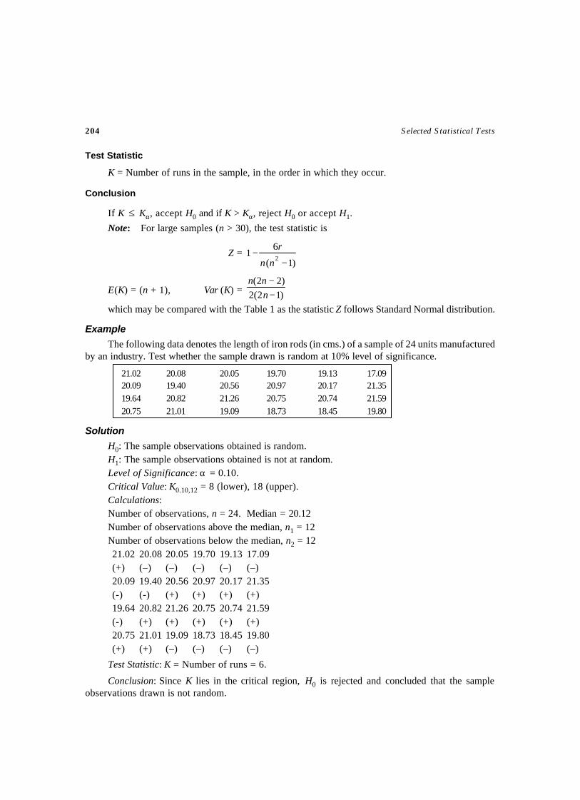
204 Selected Statistical Tests
Test Statistic
K = Number of runs in the sample, in the order in which they occur.
Conclusion
If K ≤ Kα, accept H0 and if K > Kα, reject H0 or accept H1.
Note: For large samples (n > 30), the test statistic is
Z =)1(
61
2 −−
nn
r
E(K) = (n + 1), Var (K) = )12(2)22(
−−
nnn
which may be compared with the Table 1 as the statistic Z follows Standard Normal distribution.
Example
The following data denotes the length of iron rods (in cms.) of a sample of 24 units manufacturedby an industry. Test whether the sample drawn is random at 10% level of significance.
21.02 20.08 20.05 19.70 19.13 17.0920.09 19.40 20.56 20.97 20.17 21.3519.64 20.82 21.26 20.75 20.74 21.5920.75 21.01 19.09 18.73 18.45 19.80
Solution
H0: The sample observations obtained is random.H1: The sample observations obtained is not at random.Level of Significance: α = 0.10.Critical Value: K0.10,12 = 8 (lower), 18 (upper).Calculations:Number of observations, n = 24. Median = 20.12Number of observations above the median, n1 = 12Number of observations below the median, n2 = 1221.02 20.08 20.05 19.70 19.13 17.09(+) (–) (–) (–) (–) (–)20.09 19.40 20.56 20.97 20.17 21.35(-) (-) (+) (+) (+) (+)19.64 20.82 21.26 20.75 20.74 21.59(-) (+) (+) (+) (+) (+)20.75 21.01 19.09 18.73 18.45 19.80(+) (+) (–) (–) (–) (–)
Test Statistic: K = Number of runs = 6.
Conclusion: Since K lies in the critical region, H0 is rejected and concluded that the sampleobservations drawn is not random.
Aim
To test the fluctuations in a sample have a random nature.
Source
A sample of n observations is drawn as a time series data.
Null Hypothesis
H0: The fluctuation in the sample is random.
Alternative Hypothesis
H1: The fluctuation in the sample is not random.
Level of Significance (αα) and Critical Value (Z αα )
The critical values Zα for level of significance α , are obtained from Table 1.
Method
1. The observations in the sample be given serial numbers in the order in which they occur andthey are denoted by Xi, i = 1, 2, …, n.
2. The ranks are given to the observations according to the increasing order of magnitude andis denoted by Yi, i = 1, 2, …, n.
3. Find di = Xi – Yi, i = 1, 2, …, n.
4. Find ∑=
n
iid
1
2 and denote it by r.
Test Statistic
Z =1)1(
)1(6 2
−+
−−
nnn
nnr
The statistic Z follows standard Normal distribution.
TEST FOR RANDOMNESS OF RANKCORRELATION
TEST – 54
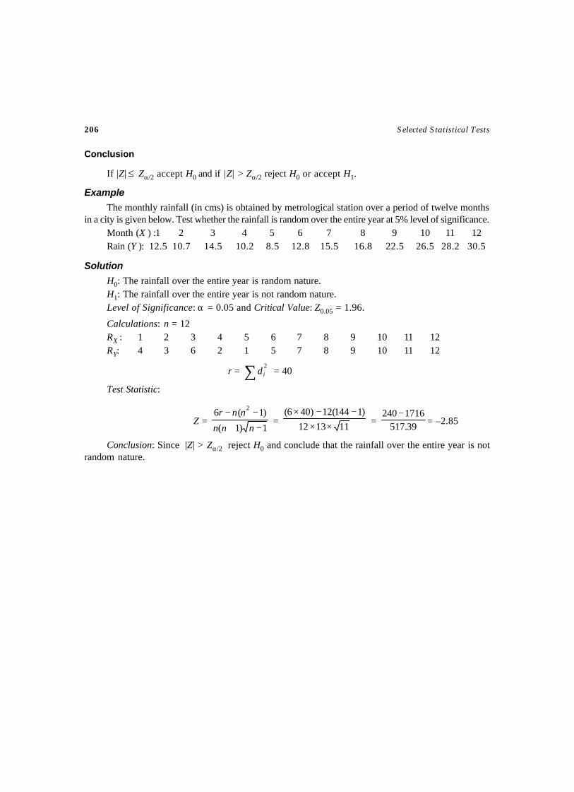
206 Selected Statistical Tests
Conclusion
If |Z| ≤ Zα/2 accept H0 and if |Z| > Zα/2 reject H0 or accept H1.
Example
The monthly rainfall (in cms) is obtained by metrological station over a period of twelve monthsin a city is given below. Test whether the rainfall is random over the entire year at 5% level of significance.
Month (X ) :1 2 3 4 5 6 7 8 9 10 11 12Rain (Y ): 12.5 10.7 14.5 10.2 8.5 12.8 15.5 16.8 22.5 26.5 28.2 30.5
Solution
H0: The rainfall over the entire year is random nature.H1: The rainfall over the entire year is not random nature.Level of Significance: α = 0.05 and Critical Value: Z0.05 = 1.96.
Calculations: n = 12RX : 1 2 3 4 5 6 7 8 9 10 11 12RY: 4 3 6 2 1 5 7 8 9 10 11 12
r = ∑ 2id = 40
Test Statistic:
Z = 1)1(
)1(6 2
−+
−−
nnn
nnr = 111312
)1144(12)406(
××−−×
= 39.5171716240 −
= –2.85
Conclusion: Since |Z| > Zα/2 reject H0 and conclude that the rainfall over the entire year is notrandom nature.

Aim
To test the significance of the differences in response for K treatments applied to n subjects.
Source
The data are obtained as a two-way table having n rows (subjects) and K columns (treatments).
Assumptions
(i) The response to one treatment by a subject is not affected by the same subject’s response toanother treatment.
(ii) The response distribution is continuous for each subject.
Null Hypothesis
H0: The effects of the K treatments are same.
Alternative Hypothesis
H1: The effects of the K treatments are not same.
Level of Significance (αα ) and Critical Value (χχ2αα )
The critical value χ2α,(K–1), for level of significance α is obtained from Table 3.
Method
1. The data be represented by a table of n rows and K columns.2. The rank numbers 1, 2,…, K are assigned in increasing order of magnitude for the values in
each row.3. The rank sum Rj, (j = 1, 2,…, K) is calculated for each of the K columns.
FRIEDMAN'S TEST FOR MULTIPLETRETMENT OF A SERIES OF OBJECTS
TEST – 55
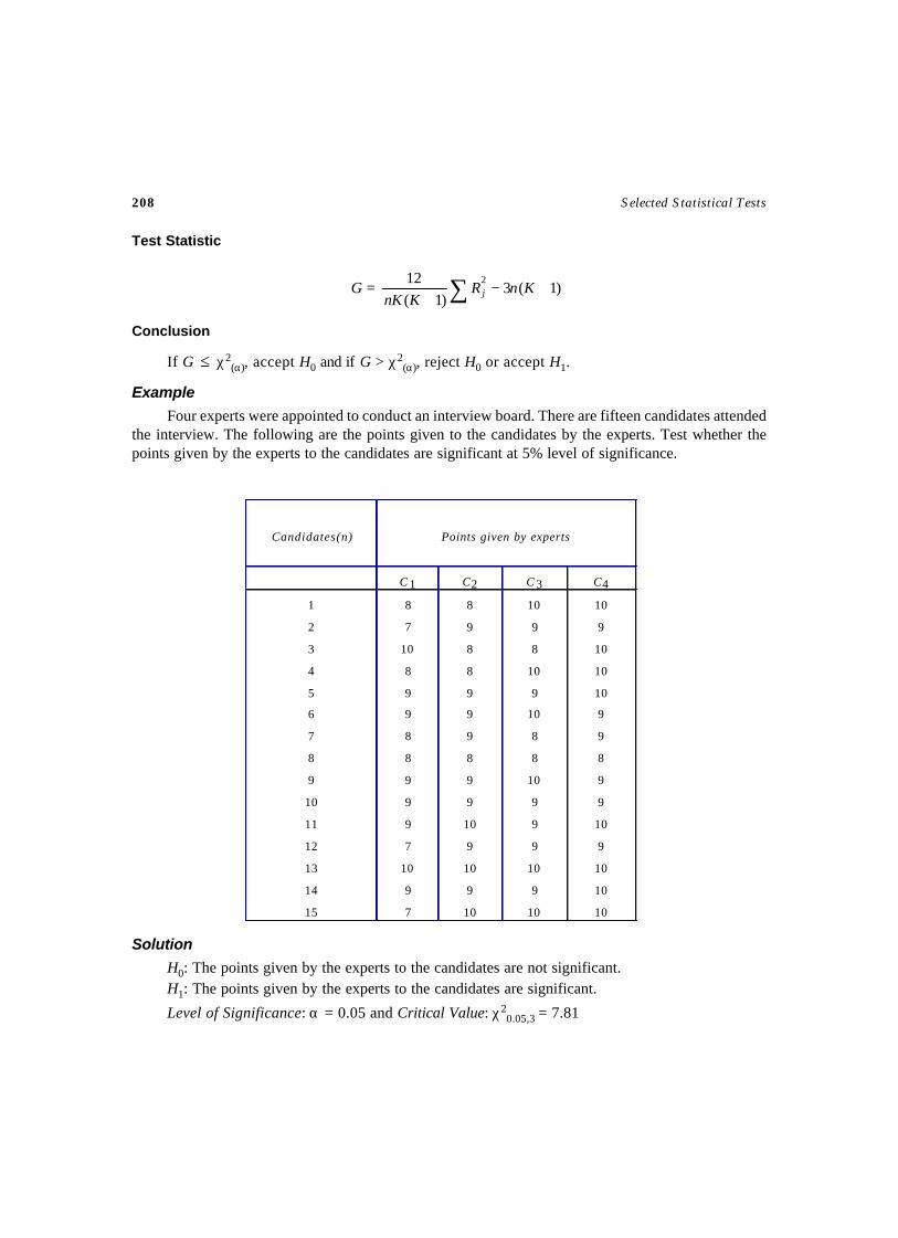
208 Selected Statistical Tests
Test Statistic
G = )1(3)1(
12 2+−
+ ∑ KnRKnK j
Conclusion
If G ≤ χ2(α), accept H0 and if G > χ2
(α), reject H0 or accept H1.
Example
Four experts were appointed to conduct an interview board. There are fifteen candidates attendedthe interview. The following are the points given to the candidates by the experts. Test whether thepoints given by the experts to the candidates are significant at 5% level of significance.
Solution
H0: The points given by the experts to the candidates are not significant.H1: The points given by the experts to the candidates are significant.
Level of Significance: α = 0.05 and Critical Value: χ20.05,3 = 7.81
Candidates(n)
Points given by experts
C 1 C2 C 3 C4
1
2
3
4
5
6
7
8
9
10
11
12
13
14
15
8
7
10
8
9
9
8
8
9
9
9
7
10
9
7
8
9
8
8
9
9
9
8
9
9
10
9
10
9
10
10
9
8
10
9
10
8
8
10
9
9
9
10
9
10
10
9
10
10
10
9
9
8
9
9
10
9
10
10
10
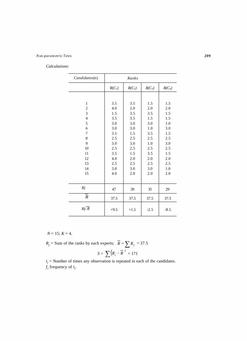
Non-parametric Tests 209
Calculations:
N = 15; K = 4.
Rj = Sum of the ranks by each experts; ∑= jRR = 37.5
S = ( )2∑ − RR j = 171
ti = Number of times any observation is repeated in each of the candidates.f i frequency of ti.
R(C1) R(C2) R(C3) R(C4)
1 2 3 4 5 6 7 8 9 10 11 12 13 14 15
3.5 4.0 1.5 3.5 3.0 3.0 3.5 2.5 3.0 2.5 3.5 4.0 2.5 3.0 4.0
3.5 2.0 3.5 3.5 3.0 3.0 1.5 2.5 3.0 2.5 1.5 2.0 2.5 3.0 2.0
1.5 2.0 3.5 1.5 3.0 1.0 3.5 2.5 1.0 2.5 3.5 2.0 2.5 3.0 2.0
1.5 2.0 1.5 1.5 1.0 3.0 1.5 2.5 3.0 2.5 1.5 2.0 2.5 1.0 2.0
47 39 35 29
R
37.5 37.5 37.5 37.5
+9.5 +1.5 -2.5 -8.5
Candidates(n) Ranks
Rj
Rj–R
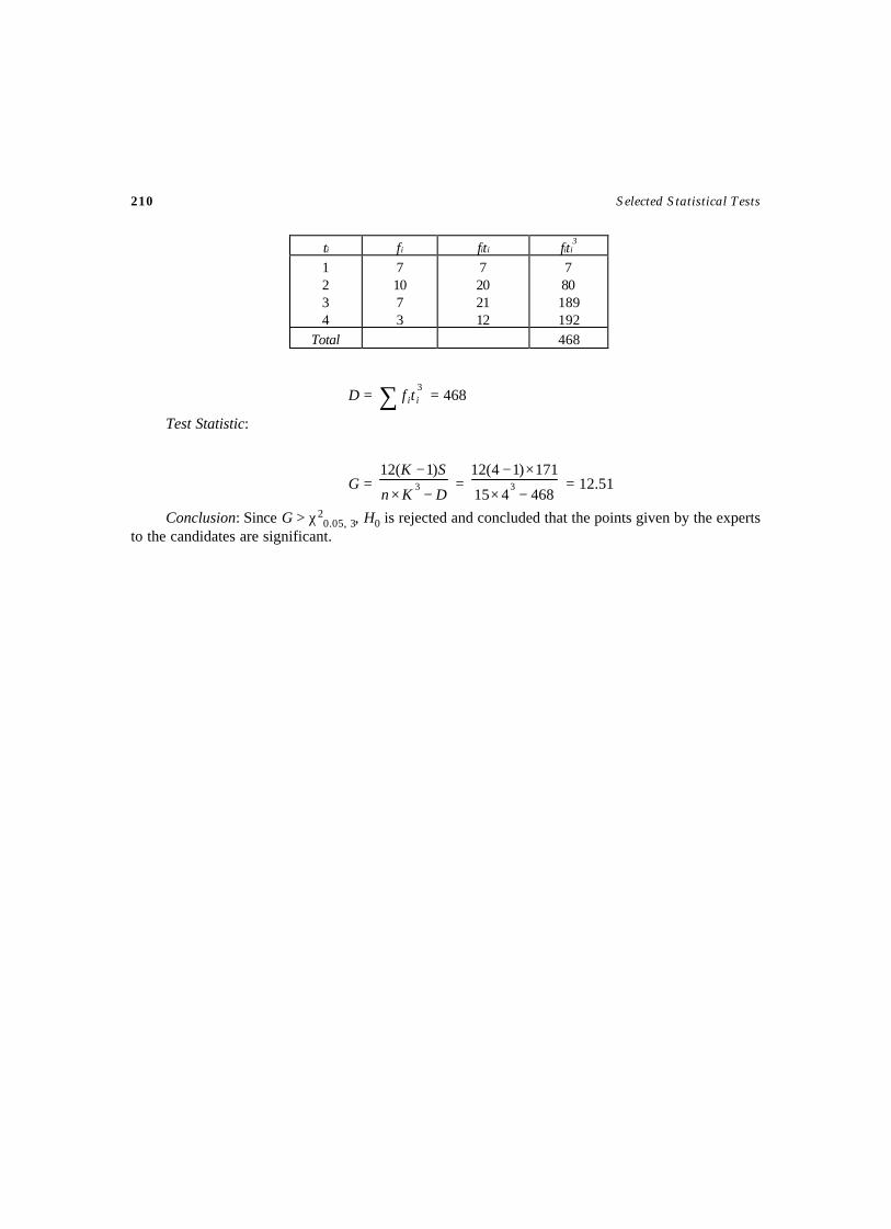
210 Selected Statistical Tests
ti fi fiti fiti3
1 2 3 4
7 10 7 3
7 20 21 12
7 80 189 192
Total 468
D = ∑ 3iitf = 468
Test Statistic:
G =DKn
SK
−×
−3
)1(12 =
468415
171)14(123
−×
×− = 12.51
Conclusion: Since G > χ20.05, 3, H0 is rejected and concluded that the points given by the experts
to the candidates are significant.

SEQUENTIAL TESTS
CHAPTER – 6

This pageintentionally left
blank
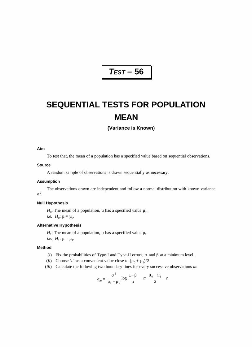
SEQUENTIAL TESTS FOR POPULATION
MEAN(Variance is Known)
TEST – 56
Aim
To test that, the mean of a population has a specified value based on sequential observations.
Source
A random sample of observations is drawn sequentially as necessary.
Assumption
The observations drawn are independent and follow a normal distribution with known varianceσ2.
Null Hypothesis
H0: The mean of a population, µ has a specified value µ0.i.e., H0: µ = µ0.
Alternative Hypothesis
H1: The mean of a population, µ has a specified value µ1.i.e., H1: µ = µ1.
Method
(i) Fix the probabilities of Type-I and Type-II errors, α and β at a minimum level.(ii) Choose ‘c’ as a convenient value close to (µ0 + µ1)/2 .
(iii) Calculate the following two boundary lines for every successive observations m:
am =
−
µ+µ+
αβ−
µ−µσ
cm2
1log 10
01
2
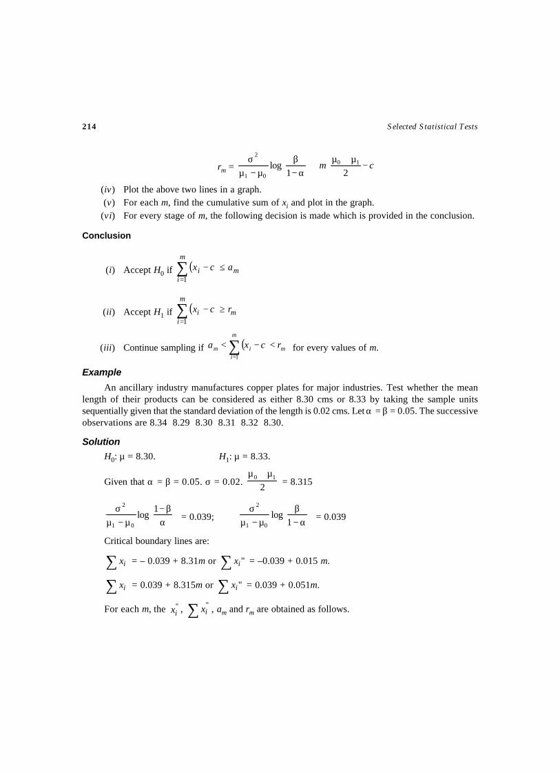
214 Selected Statistical Tests
rm =
−
µ+µ+
α−β
µ−µσ
cm21
log 10
01
2
(iv) Plot the above two lines in a graph.(v) For each m, find the cumulative sum of xi and plot in the graph.
(vi) For every stage of m, the following decision is made which is provided in the conclusion.
Conclusion
(i) Accept H0 if ( ) m
m
ii acx ≤−∑
=1
(ii) Accept H1 if ( ) m
m
ii rcx ≥−∑
=1
(iii) Continue sampling if ( ) m
m
iim rcxa <−< ∑
=1 for every values of m.
Example
An ancillary industry manufactures copper plates for major industries. Test whether the meanlength of their products can be considered as either 8.30 cms or 8.33 by taking the sample unitssequentially given that the standard deviation of the length is 0.02 cms. Let α = β = 0.05. The successiveobservations are 8.34 8.29 8.30 8.31 8.32 8.30.
Solution
H0: µ = 8.30. H1: µ = 8.33.
Given that α = β = 0.05. σ = 0.02. 210 µ+µ
= 8.315
αβ−
µ−µσ 1
log01
2
= 0.039;
α−β
µ−µσ
1log
01
2
= 0.039
Critical boundary lines are:
∑ ix = – 0.039 + 8.31m or "∑ ix = –0.039 + 0.015 m.
∑ ix = 0.039 + 8.315m or "∑ ix = 0.039 + 0.051m.
For each m, the ''ix , ∑ ''
ix , am and rm are obtained as follows.
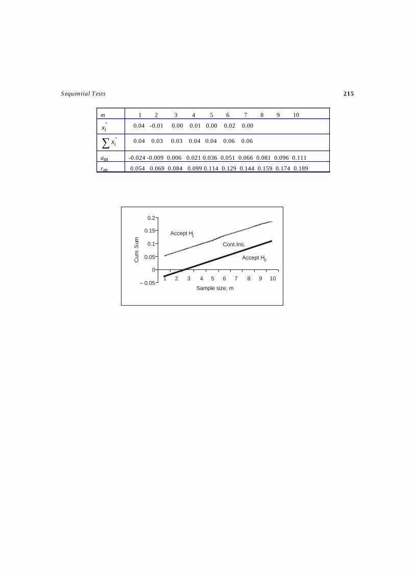
Sequential Tests 215
m 1 2 3 4 5 6 7 8 9 10
''ix
0.04 -0.01 0.00 0.01 0.00 0.02 0.00
∑ ''ix
0.04 0.03 0.03 0.04 0.04 0.06 0.06
am -0.024 -0.009 0.006 0.021 0.036 0.051 0.066 0.081 0.096 0.111
rm 0.054 0.069 0.084 0.099 0.114 0.129 0.144 0.159 0.174 0.189
0.2
0.15
0.1
0.05
0
– 0.051 2 3 4 5 6 7 8 9 10
Sample size, m
Accept H1
Cum
. Sum
Accept H0
Cont.Ins.
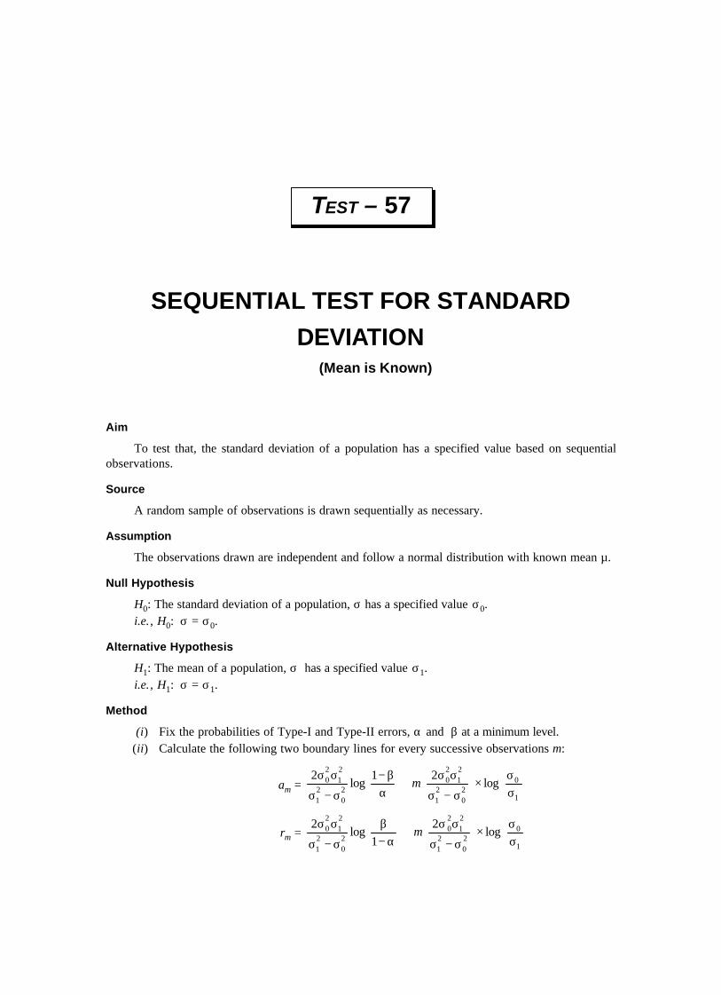
Aim
To test that, the standard deviation of a population has a specified value based on sequentialobservations.
Source
A random sample of observations is drawn sequentially as necessary.
Assumption
The observations drawn are independent and follow a normal distribution with known mean µ.
Null Hypothesis
H0: The standard deviation of a population, σ has a specified value σ0.i.e., H0: σ = σ0.
Alternative Hypothesis
H1: The mean of a population, σ has a specified value σ1.i.e., H1: σ = σ1.
Method
(i) Fix the probabilities of Type-I and Type-II errors, α and β at a minimum level.(ii) Calculate the following two boundary lines for every successive observations m:
am =
σσ
×
σ−σ
σσ+
αβ−
σ−σ
σσ
1
020
21
21
20
20
21
21
20 log
21log
2m
rm =
σσ
×
σ−σ
σσ+
α−β
σ−σ
σσ
1
020
21
21
20
20
21
21
20 log
21
log2
m
SEQUENTIAL TEST FOR STANDARD
DEVIATION(Mean is Known)
TEST – 57
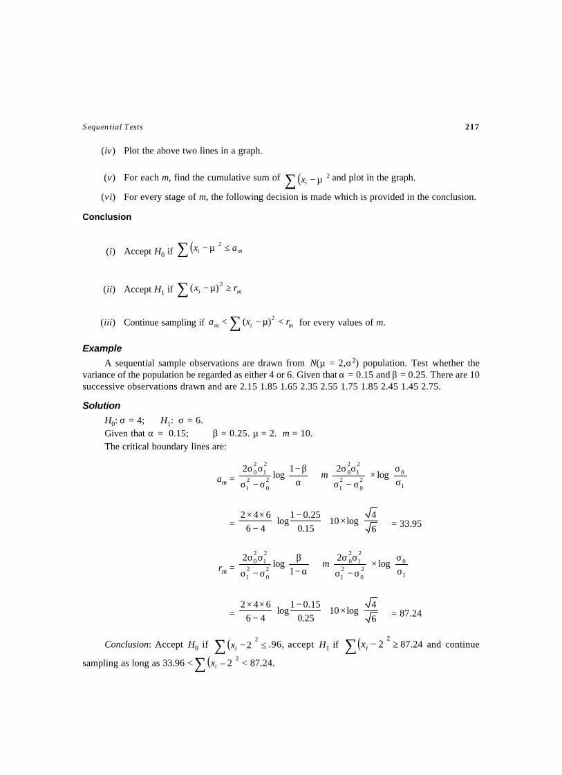
Sequential Tests 217
(iv) Plot the above two lines in a graph.
(v) For each m, find the cumulative sum of ( )∑ µ− 2ix and plot in the graph.
(vi) For every stage of m, the following decision is made which is provided in the conclusion.
Conclusion
(i) Accept H0 if ( )∑ ≤µ− mi ax 2
(ii) Accept H1 if ∑ ≥µ− mi rx 2)(
(iii) Continue sampling if ∑ <µ−< mim rxa 2)( for every values of m.
Example
A sequential sample observations are drawn from N(µ = 2,σ2) population. Test whether thevariance of the population be regarded as either 4 or 6. Given that α = 0.15 and β = 0.25. There are 10successive observations drawn and are 2.15 1.85 1.65 2.35 2.55 1.75 1.85 2.45 1.45 2.75.
Solution
H0: σ = 4; H1: σ = 6.Given that α = 0.15; β = 0.25. µ = 2. m = 10.The critical boundary lines are:
am =
σσ
×
σ−σ
σσ+
αβ−
σ−σ
σσ
1
020
21
21
20
20
21
21
20 log
21log
2m
=
×+
−−
××6
4log10
15.025.01
log46
642 = 33.95
rm =
σσ
×
σ−σ
σσ+
α−β
σ−σ
σσ
1
020
21
21
20
20
21
21
20 log
21
log2
m
=
×+
−−
××6
4log10
25.015.01
log46
642 = 87.24
Conclusion: Accept H0 if ( ) ≤−∑ 22ix .96, accept H1 if ( ) ≥−∑ 2
2ix 87.24 and continue
sampling as long as 33.96 < ( )∑ 22–ix < 87.24.
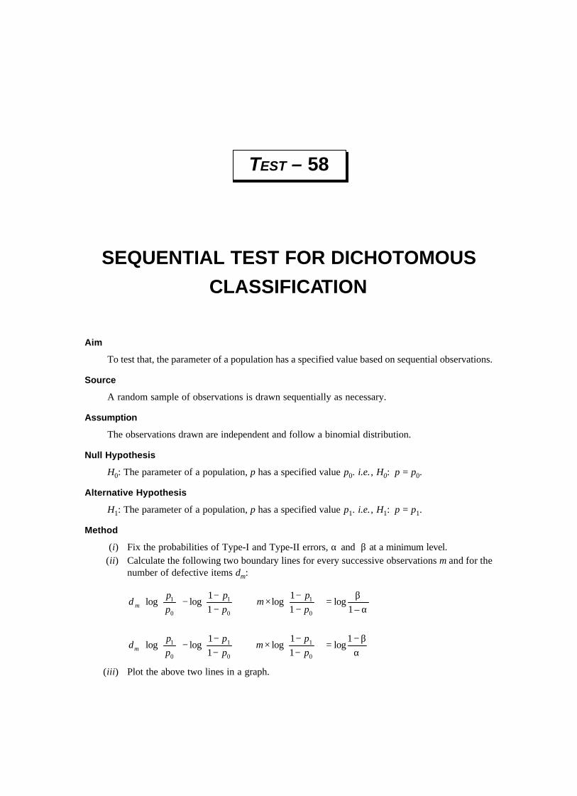
Aim
To test that, the parameter of a population has a specified value based on sequential observations.
Source
A random sample of observations is drawn sequentially as necessary.
Assumption
The observations drawn are independent and follow a binomial distribution.
Null Hypothesis
H0: The parameter of a population, p has a specified value p0. i.e., H0: p = p0.
Alternative Hypothesis
H1: The parameter of a population, p has a specified value p1. i.e., H1: p = p1.
Method
(i) Fix the probabilities of Type-I and Type-II errors, α and β at a minimum level.(ii) Calculate the following two boundary lines for every successive observations m and for the
number of defective items dm:
αβ
=
−−
×+
−−
−
–1
log11
log11
loglog0
1
0
1
0
1
pp
mpp
pp
d m
αβ−
=
−−
×+
−−
−
1log
11
log11
loglog0
1
0
1
0
1
pp
mpp
pp
dm
(iii) Plot the above two lines in a graph.
SEQUENTIAL TEST FOR DICHOTOMOUS
CLASSIFICATION
TEST – 58
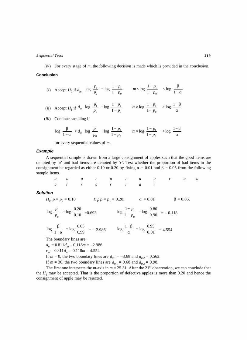
Sequential Tests 219
(iv) For every stage of m, the following decision is made which is provided in the conclusion.
Conclusion
(i) Accept H0 if dm
α−β
≤
−−
×+
−−
−
1
log11
log11
loglog0
1
0
1
0
1
pp
mpp
pp
(ii) Accept H1 if
αβ−
≥
−−
×+
−−
−
1log
11
log11
loglog0
1
0
1
0
1
pp
mpp
pp
dm
(iii) Continue sampling if
αβ−
<
−−
×+
−−
−
<
α−β 1
log11
log11
loglog1
log0
1
0
1
0
1
pp
mpp
pp
dm
for every sequential values of m.
Example
A sequential sample is drawn from a large consignment of apples such that the good items aredenoted by ‘a’ and bad items are denoted by ‘r’. Test whether the proportion of bad items in theconsignment be regarded as either 0.10 or 0.20 by fixing α = 0.01 and β = 0.05 from the followingsample items.
a a a r a r a a r a aa r r a r r a r
Solution
H0: p = p0 = 0.10 H1: p = p1 = 0.20; α = 0.01 β = 0.05.
=
10.020.0
loglog0
1
p
p=0.693
=
−−
90.080.0
log1
1log
0
1
p
p = – 0.118
=
α−β
99.005.0
log1
log = – 2.986
=
αβ−
01.095.0
log1
log = 4.554
The boundary lines are:am = 0.811dm – 0.118m = –2.986rm = 0.811dm – 0.118m = 4.554If m = 0, the two boundary lines are dm1 = –3.68 and dm2 = 0.562.If m = 30, the two boundary lines are dm1 = 0.68 and dm2 = 9.98.The first one intersects the m-axis in m = 25.31. After the 21st observation, we can conclude that
the H1 may be accepted. That is the proportion of defective apples is more than 0.20 and hence theconsignment of apple may be rejected.
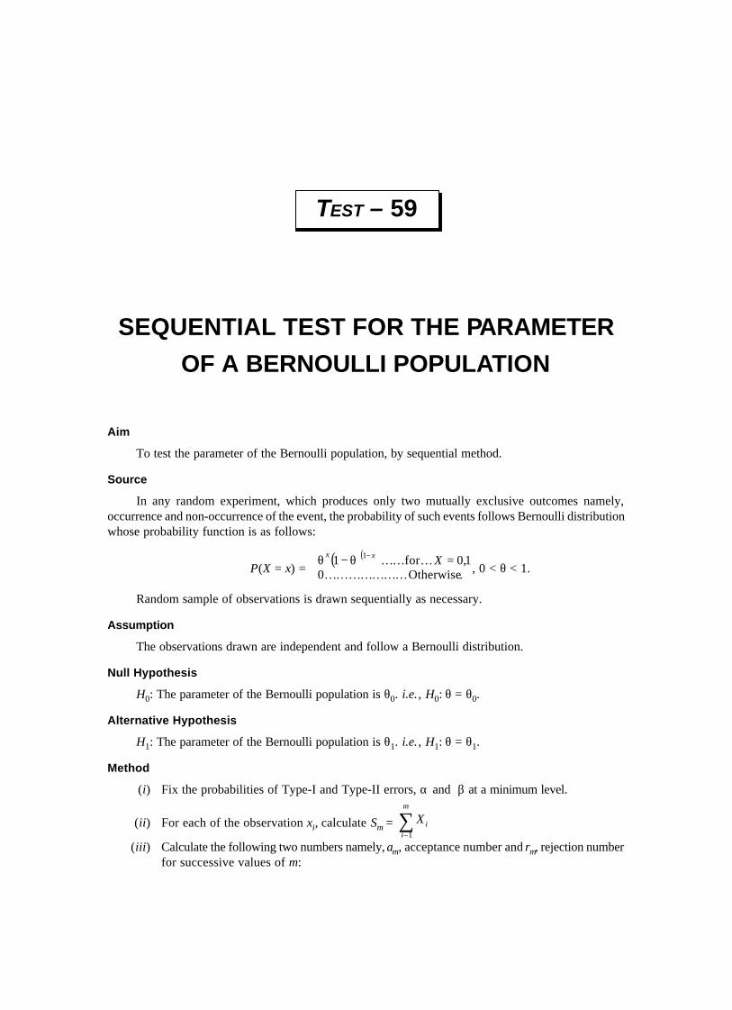
Aim
To test the parameter of the Bernoulli population, by sequential method.
Source
In any random experiment, which produces only two mutually exclusive outcomes namely,occurrence and non-occurrence of the event, the probability of such events follows Bernoulli distributionwhose probability function is as follows:
P(X = x) =( )( )
=θ−θ −
.Otherwise01,0for1 1
………………………… Xxx
, 0 < θ < 1.
Random sample of observations is drawn sequentially as necessary.
Assumption
The observations drawn are independent and follow a Bernoulli distribution.
Null Hypothesis
H0: The parameter of the Bernoulli population is θ0. i.e., H0: θ = θ0.
Alternative Hypothesis
H1: The parameter of the Bernoulli population is θ1. i.e., H1: θ = θ1.
Method
(i) Fix the probabilities of Type-I and Type-II errors, α and β at a minimum level.
(ii) For each of the observation xi, calculate Sm = ∑m
iiX
1–
(iii) Calculate the following two numbers namely, am, acceptance number and rm, rejection numberfor successive values of m:
SEQUENTIAL TEST FOR THE PARAMETER
OF A BERNOULLI POPULATION
TEST – 59
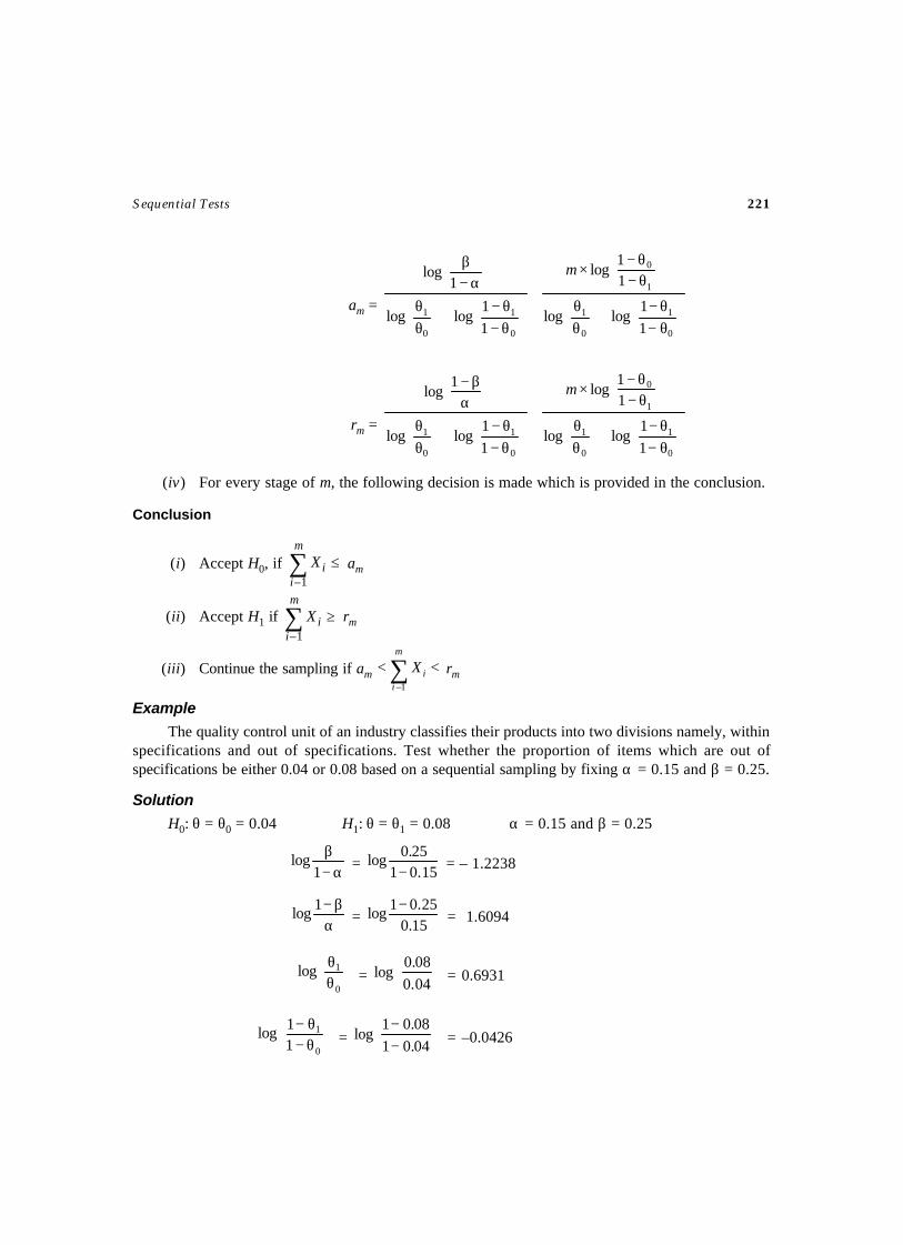
Sequential Tests 221
am =
θ−θ−
+
θθ
θ−θ−
×+
θ−θ−
+
θθ
α−β
0
1
0
1
1
0
0
1
0
1
11
loglog
11
log
11
loglog
1log m
rm =
θ−θ−
+
θθ
θ−θ−
×+
θ−θ−
+
θθ
αβ−
0
1
0
1
1
0
0
1
0
1
11
loglog
11
log
11
loglog
1log m
(iv) For every stage of m, the following decision is made which is provided in the conclusion.
Conclusion
(i) Accept H0, if ≤∑m
iiX
1–
am
(ii) Accept H1 if ≥∑m
iiX
1–
rm
(iii) Continue the sampling if am << ∑m
iiX
1– rm
Example
The quality control unit of an industry classifies their products into two divisions namely, withinspecifications and out of specifications. Test whether the proportion of items which are out ofspecifications be either 0.04 or 0.08 based on a sequential sampling by fixing α = 0.15 and β = 0.25.
Solution
H0: θ = θ0 = 0.04 H1: θ = θ1 = 0.08 α = 0.15 and β = 0.25
α−β
1log = 15.01
25.0log− = – 1.2238
αβ−1log = 15.0
25.01log −= 1.6094
θθ
0
1log =
04.008.0
log = 0.6931
θ−θ−
0
1
11log =
−−
04.0108.01
log = –0.0426
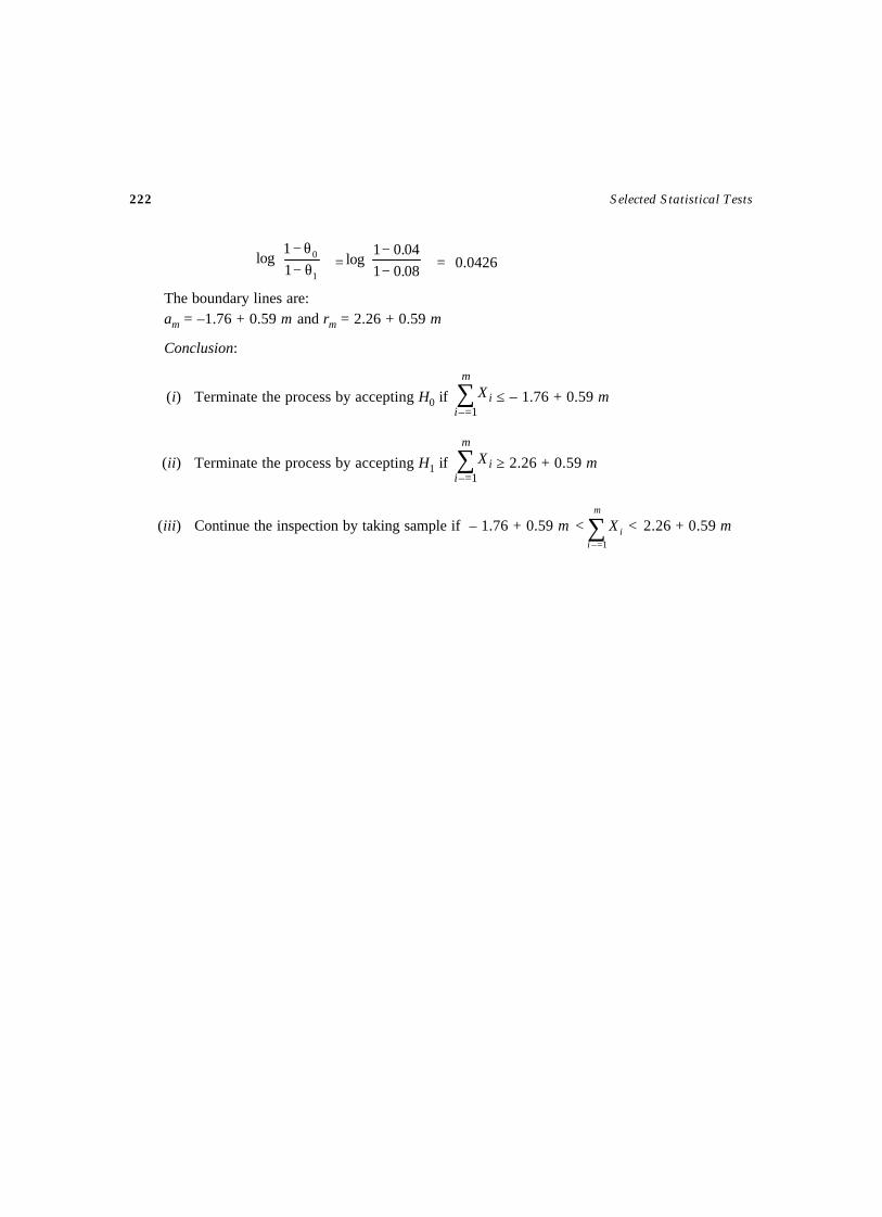
222 Selected Statistical Tests
θ−θ−
1
0
11
log =
−−
08.0104.01
log = 0.0426
The boundary lines are:am = –1.76 + 0.59 m and rm = 2.26 + 0.59 m
Conclusion:
(i) Terminate the process by accepting H0 if ∑=
m
iiX
1–≤ – 1.76 + 0.59 m
(ii) Terminate the process by accepting H1 if ∑=
m
iiX
1–≥ 2.26 + 0.59 m
(iii) Continue the inspection by taking sample if – 1.76 + 0.59 m << ∑=
m
iiX
1–
2.26 + 0.59 m
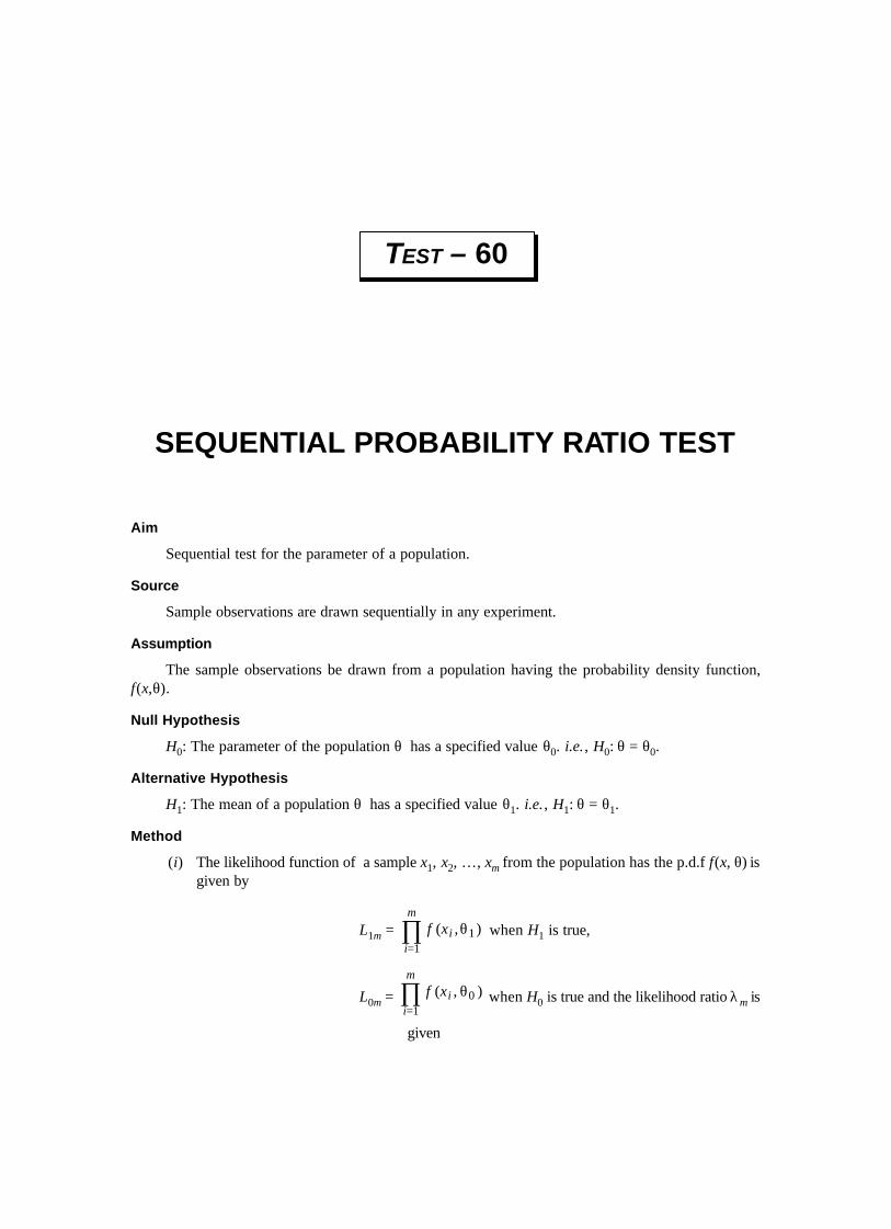
Aim
Sequential test for the parameter of a population.
Source
Sample observations are drawn sequentially in any experiment.
Assumption
The sample observations be drawn from a population having the probability density function,f(x,θ).
Null Hypothesis
H0: The parameter of the population θ has a specified value θ0. i.e., H0: θ = θ0.
Alternative Hypothesis
H1: The mean of a population θ has a specified value θ1. i.e., H1: θ = θ1.
Method
(i) The likelihood function of a sample x1, x2, …, xm from the population has the p.d.f f(x, θ) isgiven by
L1m = ∏=
θm
iixf
11),( when H1 is true,
L0m = ∏=
θm
iixf
10 ),( when H0 is true and the likelihood ratio λm is
given
SEQUENTIAL PROBABILITY RATIO TEST
TEST – 60
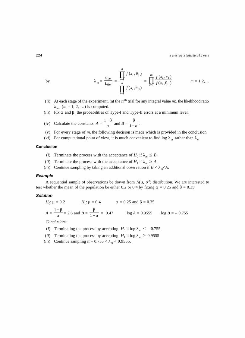
224 Selected Statistical Tests
by λm =m
m
L
L
0
1 =
∏
∏
=
=
θ
θ
n
ii
n
ii
xf
xf
10
11
),(
),(
= ∏= θ
θm
i i
i
xf
xf
1 0
1
),(
),(m = 1,2,…
(ii) At each stage of the experiment, (at the mth trial for any integral value m), the likelihood ratioλm , (m = 1, 2, …) is computed.
(iii) Fix α and β, the probabilities of Type-I and Type-II errors at a minimum level.
(iv) Calculate the constants, A = αβ−1
and B = α−β
1 .
(v) For every stage of m, the following decision is made which is provided in the conclusion.(vi) For computational point of view, it is much convenient to find log λm rather than λm.
Conclusion
(i) Terminate the process with the acceptance of H0 if λm ≤ B.
(ii) Terminate the process with the acceptance of H1 if λm ≥ A.(iii) Continue sampling by taking an additional observation if B < λm<A.
Example
A sequential sample of observations be drawn from N(µ, σ2) distribution. We are interested totest whether the mean of the population be either 0.2 or 0.4 by fixing α = 0.25 and β = 0.35.
Solution
H0: µ = 0.2 H1: µ = 0.4 α = 0.25 and β = 0.35
A = αβ−1
= 2.6 and B = α−β
1 = 0.47 log A = 0.9555 log B = – 0.755
Conclusions:
(i) Terminating the process by accepting H0 if log λm ≤ – 0.755
(ii) Terminating the process by accepting H1 if log λm ≥ 0.9555(iii) Continue sampling if – 0.755 < λm < 0.9555.

TABLES
CHAPTER – 7
Table 1 The area under the normal curve.
Table 2 Critical values of t distribution.
Table 3 Area in the right tail of a chi-square ( χ2) distribution.
Table 4 Critical values of f distribution with α = 0.05 and α = 0.01 of the area inthe right tail.
Table 5 Critical values of t for the sign test.
Table 6 Critical values of r for the sign test.
Table 7 Critical values of r in the Wald-Wolfwitz two sample runs test.
Table 8 Critical values of the smallest rank sum for the Wilcoxon-Mann-Whitneytest.
Table 9 Critical values of the Kolmogorov-Smirnov one sample test statistics.
Table 10 Critical values of rs for the spearman rank correlation test.
Table 11 Critical values for the run test (equal sample sizes).
TABLES

Tables 227
TABLE 1: THE AREA UNDER THE NORMAL CURVE
Z 0.00 0.01 0.02 0.03 0.04 0.05 0.06 0.07 0.08 0.09
-3.4 0.0003 0.0003 0.0003 0.0003 0.0003 0.0003 0.0003 0.0003 0.0003 0.0002 -3.3 0.0005 0.0005 0.0005 0.0004 0.0004 0.0004 0.0004 0.0004 0.0004 0.0003 -3.2 0.0007 0.0007 0.0006 0.0006 0.0006 0.0006 0.0006 0.0005 0.0005 0.0005 -3.1 0.0010 0.0009 0.0009 0.0009 0.0008 0.0008 0.0008 0.0008. 0.0007 0.0007 -3.0 0.0013 0.0013 0.0013 0.0012 0.0012 0.0011 0.0011 0.0011 0.0010 0.0010
-2.9 9990.0019 0.0018 0.0017 0.0017 0.0016 0.0016 0.0015 0.0015 0.0014 0.0014 -2.8 0.0026 0.0025 0.0024 0.0023 0.0023 0.0022 0.0021 0.0021 0.0020 0.0019 -2.7 0.0035 0.0033 0.0033 0.0032 0.0031 0.0030 0.0029 0.0028 0.0027 0.0026 -2.6 0.0047 0.0045 0.0044 0.0043 0.0041 0.0040 0.0039 0.0038 0.0037 0.0036 -2.5 0.0062 0.0060 0.0059 0.0057 0.0055 0.0054 0.0052 0.0051 0.0049 0.0048
-2.4 0.0082 0.0080 0.0078 0.0075 0.0073 0.0071 0.0069 0.0068 0.0066 0.0064 -2.3 0.0107 0.0104 0.0102 0.0099 0.0096 0.0094 0.0091 0.0089 0.0087 0.0084 -2.2 0.0139 0.0136 0.0132 0.0129 0.0125 0.0122 0.0119 0.0116 0.0113 0.0110 -2.1 0.0179 0.0114 0.0170 0.0166 0.0162 0.0158 0.0154 0.0150 0.0146 0.0143 -2.0 0.0228 0.0222 0.0217 0.0212 0.0207 0.0202 0.0197 0.0192 0.0188 0.0183
-1.9 0.0287 0.0281 0.0274 0.0268 0.0262 0.0256 0.0250 0.0244 0.0239 0.0233 -1.8 0.0359 0.0352 0.0344 0.0336 0.0329 0.0322 0.0314 0.0307 0.0301 0.0294 -1.7 0.0446 0.0436 0.0427 0.0418 0.0409 0.0401 0.0392 0.0384 0.0375 0.0367 -1.6 0.0548 0.0537 0.0526 0.0516 0.0505 0.0495 0.0485 0.0475 0.0465 0.0455 -1.5 0.0668 0.0655 0.0643 0.0630 0.0618 0.0606 0.0594 0.0582 0.0571 0.0559
-1.4 0.0808 0.0793 0.0778 0.0764 0.0749 0.0735 0.0722 0.0708 0.0694 0.0681 -1.3 0.0968 0.0951 0.0934 0.0918 0.0901 0.0885 0.0869 0.0853 0.0838 0.0823 -1.2 0.1151 0.1131 0.1112 0.1093 0.1075 0.1056 0.1038 0.1020 0.1003 0.0985 -1.1 0.1357 0.1335 0.1314 0.1292 0.1271 0.1251 0.1230 0.1210 0.1190 0.1170 - 1.0 0.1587 0.1562 0.1539 0.1515 0.1492 0.1469 0.1446 0.1423 0.1401 0.1379
-0.9 0.1841 0.1814 0.1788 0.1762 0.1736 0.1711 0.1685 0.1660 0.1635 0.1611 -0.8 0.2119 0.2090 0.2061 0.2033 0.2005 0.1977 0.1949 0.1922 0.1894 0.1867
Area
(Contd...)
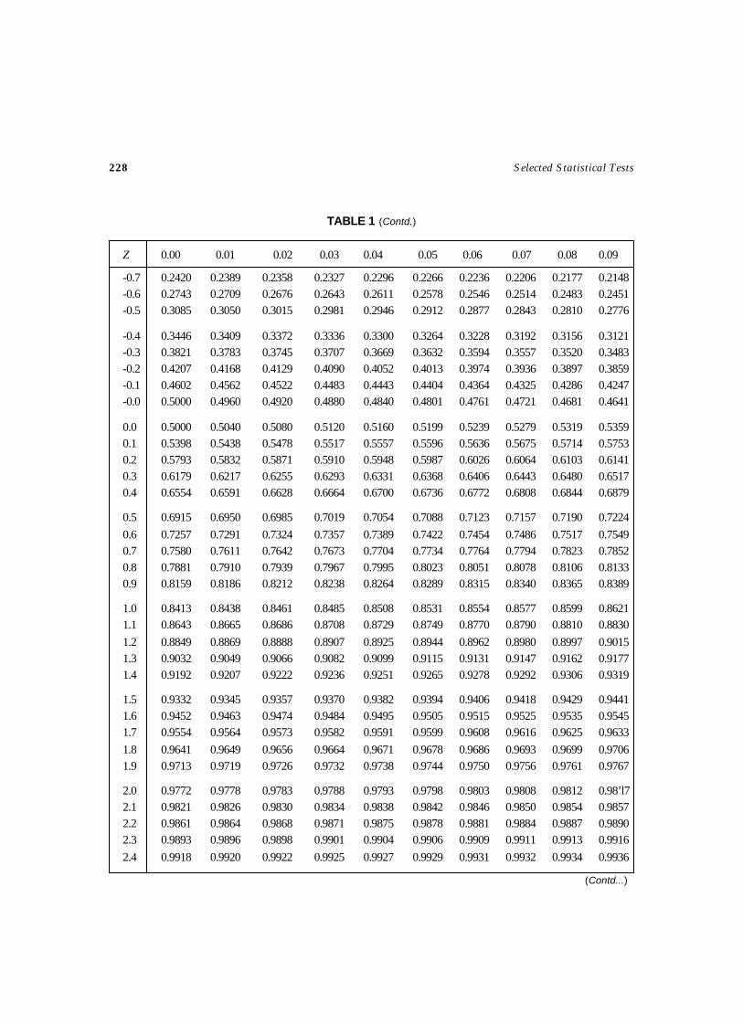
228 Selected Statistical Tests
TABLE 1 (Contd.)
Z 0.00 0.01 0.02 0.03 0.04 0.05 0.06 0.07 0.08 0.09
-0.7 0.2420 0.2389 0.2358 0.2327 0.2296 0.2266 0.2236 0.2206 0.2177 0.2148-0.6 0.2743 0.2709 0.2676 0.2643 0.2611 0.2578 0.2546 0.2514 0.2483 0.2451-0.5 0.3085 0.3050 0.3015 0.2981 0.2946 0.2912 0.2877 0.2843 0.2810 0.2776
-0.4 0.3446 0.3409 0.3372 0.3336 0.3300 0.3264 0.3228 0.3192 0.3156 0.3121-0.3 0.3821 0.3783 0.3745 0.3707 0.3669 0.3632 0.3594 0.3557 0.3520 0.3483-0.2 0.4207 0.4168 0.4129 0.4090 0.4052 0.4013 0.3974 0.3936 0.3897 0.3859-0.1 0.4602 0.4562 0.4522 0.4483 0.4443 0.4404 0.4364 0.4325 0.4286 0.4247-0.0 0.5000 0.4960 0.4920 0.4880 0.4840 0.4801 0.4761 0.4721 0.4681 0.4641
0.0 0.5000 0.5040 0.5080 0.5120 0.5160 0.5199 0.5239 0.5279 0.5319 0.53590.1 0.5398 0.5438 0.5478 0.5517 0.5557 0.5596 0.5636 0.5675 0.5714 0.57530.2 0.5793 0.5832 0.5871 0.5910 0.5948 0.5987 0.6026 0.6064 0.6103 0.61410.3 0.6179 0.6217 0.6255 0.6293 0.6331 0.6368 0.6406 0.6443 0.6480 0.65170.4 0.6554 0.6591 0.6628 0.6664 0.6700 0.6736 0.6772 0.6808 0.6844 0.6879
0.5 0.6915 0.6950 0.6985 0.7019 0.7054 0.7088 0.7123 0.7157 0.7190 0.7224
0.6 0.7257 0.7291 0.7324 0.7357 0.7389 0.7422 0.7454 0.7486 0.7517 0.75490.7 0.7580 0.7611 0.7642 0.7673 0.7704 0.7734 0.7764 0.7794 0.7823 0.78520.8 0.7881 0.7910 0.7939 0.7967 0.7995 0.8023 0.8051 0.8078 0.8106 0.81330.9 0.8159 0.8186 0.8212 0.8238 0.8264 0.8289 0.8315 0.8340 0.8365 0.8389
1.0 0.8413 0.8438 0.8461 0.8485 0.8508 0.8531 0.8554 0.8577 0.8599 0.86211.1 0.8643 0.8665 0.8686 0.8708 0.8729 0.8749 0.8770 0.8790 0.8810 0.8830
1.2 0.8849 0.8869 0.8888 0.8907 0.8925 0.8944 0.8962 0.8980 0.8997 0.90151.3 0.9032 0.9049 0.9066 0.9082 0.9099 0.9115 0.9131 0.9147 0.9162 0.91771.4 0.9192 0.9207 0.9222 0.9236 0.9251 0.9265 0.9278 0.9292 0.9306 0.9319
1.5 0.9332 0.9345 0.9357 0.9370 0.9382 0.9394 0.9406 0.9418 0.9429 0.94411.6 0.9452 0.9463 0.9474 0.9484 0.9495 0.9505 0.9515 0.9525 0.9535 0.95451.7 0.9554 0.9564 0.9573 0.9582 0.9591 0.9599 0.9608 0.9616 0.9625 0.9633
1.8 0.9641 0.9649 0.9656 0.9664 0.9671 0.9678 0.9686 0.9693 0.9699 0.97061.9 0.9713 0.9719 0.9726 0.9732 0.9738 0.9744 0.9750 0.9756 0.9761 0.9767
2.0 0.9772 0.9778 0.9783 0.9788 0.9793 0.9798 0.9803 0.9808 0.9812 0.98’l72.1 0.9821 0.9826 0.9830 0.9834 0.9838 0.9842 0.9846 0.9850 0.9854 0.98572.2 0.9861 0.9864 0.9868 0.9871 0.9875 0.9878 0.9881 0.9884 0.9887 0.98902.3 0.9893 0.9896 0.9898 0.9901 0.9904 0.9906 0.9909 0.9911 0.9913 0.9916
2.4 0.9918 0.9920 0.9922 0.9925 0.9927 0.9929 0.9931 0.9932 0.9934 0.9936
(Contd...)
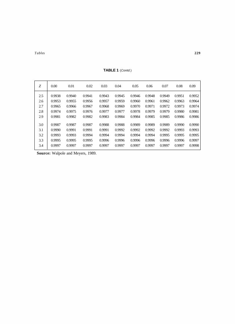
Tables 229
TABLE 1 (Contd.)
Source: Walpole and Meyers, 1989.
Z 0.00 0.01 0.02 0.03 0.04 0.05 0.06 0.07 0.08 0.09
2.5 0.9938 0.9940 0.9941 0.9943 0.9945 0.9946 0.9948 0.9949 0.9951 0.99522.6 0.9953 0.9955 0.9956 0.9957 0.9959 0.9960 0.9961 0.9962 0.9963 0.99642.7 0.9965 0.9966 0.9967 0.9968 0.9969 0.9970 0.9971 0.9972 0.9973 0.99742.8 0.9974 0.9975 0.9976 0.9977 0.9977 0.9978 0.9979 0.9979 0.9980 0.99812.9 0.9981 0.9982 0.9982 0.9983 0.9984 0.9984 0.9985 0.9985 0.9986 0.9986
3.0 0.9987 0.9987 0.9987 0.9988 0.9988 0.9989 0.9989 0.9989 0.9990 0.99903.1 0.9990 0.9991 0.9991 0.9991 0.9992 0.9992 0.9992 0.9992 0.9993 0.99933.2 0.9993 0.9993 0.9994 0.9994 0.9994 0.9994 0.9994 0.9995 0.9995 0.99953.3 0.9995 0.9995 0.9995 0.9996 0.9996 0.9996 0.9996 0.9996 0.9996 0.99973.4 0.9997 0.9997 0.9997 0.9997 0.9997 0.9997 0.9997 0.9997 0.9997 0.9998
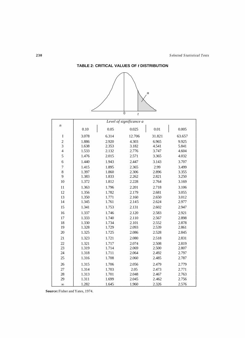
230 Selected Statistical Tests
TABLE 2: CRITICAL VALUES OF t DISTRIBUTION
Source: Fisher and Yates, 1974.
0.10 0.05 0.025 0.01 0.005
I 3.078 6.314 12.706 31.821 63.657 2 1.886 2.920 4.303 6.965 9.925 3 1.638 2.353 3.182 4.541 5.841 4 1.533 2.132 2.776 3.747 4.604 5 1.476 2.015 2.571 3.365 4.032
6 1.440 1.943 2.447 3.143 3.707 7 1.415 1.895 2.365 2.99 3.499 8 1.397 1.860 2.306 2.896 3.355 9 1.383 1.833 2.262 2.821 3.250 10 1.372 1.812 2.228 2.764 3.169
11 1.363 1.796 2.201 2.718 3.106 12 1.356 1.782 2.179 2.681 3.055 13 1.350 1.771 2.160 2.650 3.012 14 1.345 1.761 2.145 2.624 2.977 15 1.341 1.753 2.131 2.602 2.947
16 1.337 1.746 2.120 2.583 2.921 17 1.333 1.740 2.110 2.567 2.898 18 1.330 1.734 2.101 2.552 2.878 19 1.328 1.729 2.093 2.539 2.861 20 1.325 1.725 2.086 2.528 2.845
21 1.323 1.721 2.080 2.518 2.831 22 1.321 1.717 2.074 2.508 2.819 23 1.319 1.714 2.069 2.500 2.807 24 1.318 1.711 2.064 2.492 2.797 25 1.316 1.708 2.060 2.485 2.787
26 1.315 1.706 2.056 2.479 2.779 27 1.314 1.703 2.05 2.473 2.771 28 1.313 1.701 2.048 2.467 2.763 29 1.311 1.699 2.045 2.462 2.756 ∞ 1.282 1.645 1.960 2.326 2.576
nLevel of significance α
0
α
t
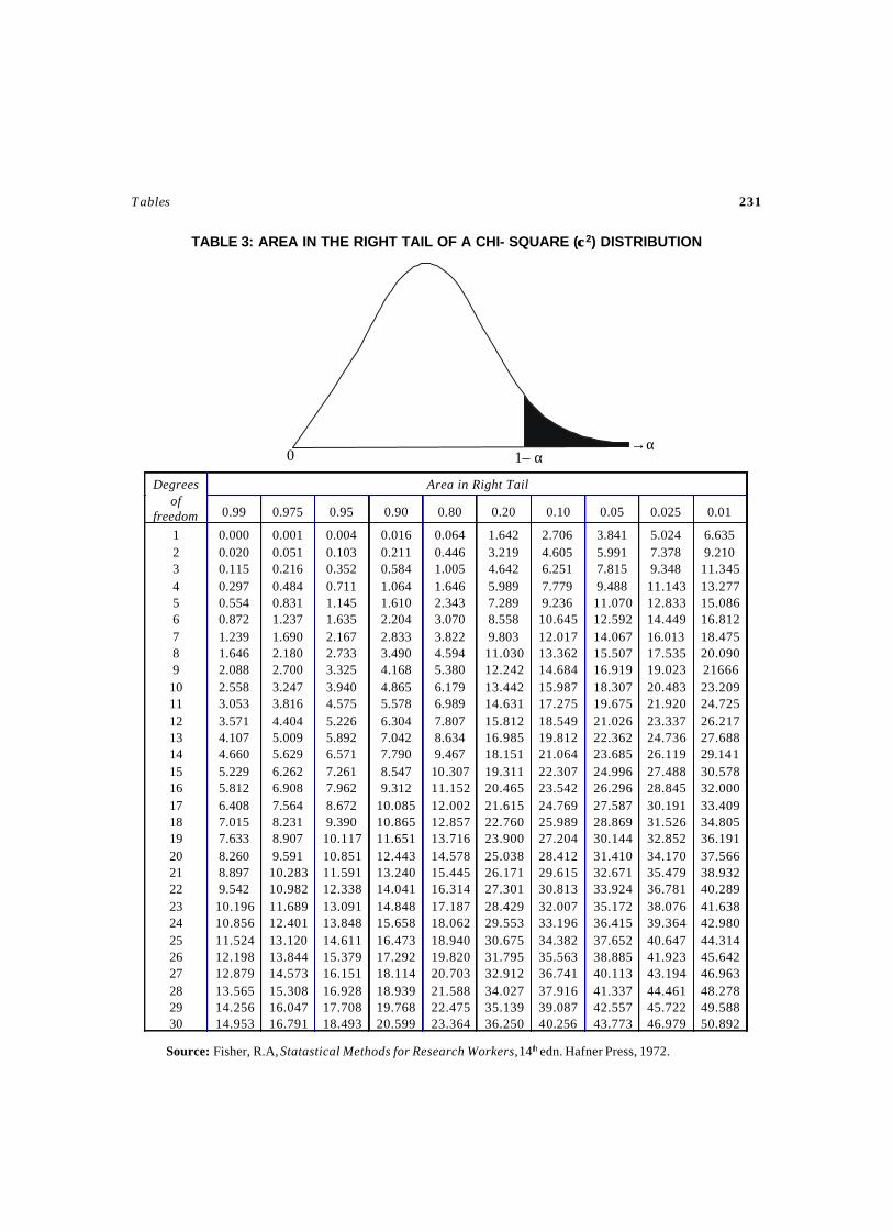
Tables 231
TABLE 3: AREA IN THE RIGHT TAIL OF A CHI- SQUARE (χχ2) DISTRIBUTION
Area in Right Tail Degrees of
freedom 0.99 0.975 0.95 0.90 0.80 0.20 0.10 0.05 0.025 0.01
1 2 3 4 5 6 7 8 9 10 11 12 13 14 15 16 17 18 19 20 21 22 23 24 25 26 27 28 29 30
0.000 0.020 0.115 0.297 0.554 0.872 1.239 1.646 2.088 2.558 3.053 3.571 4.107 4.660 5.229 5.812 6.408 7.015 7.633 8.260 8.897 9.542 10.196 10.856 11.524 12.198 12.879 13.565 14.256 14.953
0.001 0.051 0.216 0.484 0.831 1.237 1.690 2.180 2.700 3.247 3.816 4.404 5.009 5.629 6.262 6.908 7.564 8.231 8.907 9.591 10.283 10.982 11.689 12.401 13.120 13.844 14.573 15.308 16.047 16.791
0.004 0.103 0.352 0.711 1.145 1.635 2.167 2.733 3.325 3.940 4.575 5.226 5.892 6.571 7.261 7.962 8.672 9.390 10.117 10.851 11.591 12.338 13.091 13.848 14.611 15.379 16.151 16.928 17.708 18.493
0.016 0.211 0.584 1.064 1.610 2.204 2.833 3.490 4.168 4.865 5.578 6.304 7.042 7.790 8.547 9.312
10.085 10.865 11.651 12.443 13.240 14.041 14.848 15.658 16.473 17.292 18.114 18.939 19.768 20.599
0.064 0.446 1.005 1.646 2.343 3.070 3.822 4.594 5.380 6.179 6.989 7.807 8.634 9.467 10.307 11.152 12.002 12.857 13.716 14.578 15.445 16.314 17.187 18.062 18.940 19.820 20.703 21.588 22.475 23.364
1.642 3.219 4.642 5.989 7.289 8.558 9.803 11.030 12.242 13.442 14.631 15.812 16.985 18.151 19.311 20.465 21.615 22.760 23.900 25.038 26.171 27.301 28.429 29.553 30.675 31.795 32.912 34.027 35.139 36.250
2.706 4.605 6.251 7.779 9.236 10.645 12.017 13.362 14.684 15.987 17.275 18.549 19.812 21.064 22.307 23.542 24.769 25.989 27.204 28.412 29.615 30.813 32.007 33.196 34.382 35.563 36.741 37.916 39.087 40.256
3.841 5.991 7.815 9.488 11.070 12.592 14.067 15.507 16.919 18.307 19.675 21.026 22.362 23.685 24.996 26.296 27.587 28.869 30.144 31.410 32.671 33.924 35.172 36.415 37.652 38.885 40.113 41.337 42.557 43.773
5.024 7.378 9.348 11.143 12.833 14.449 16.013 17.535 19.023 20.483 21.920 23.337 24.736 26.119 27.488 28.845 30.191 31.526 32.852 34.170 35.479 36.781 38.076 39.364 40.647 41.923 43.194 44.461 45.722 46.979
6.635 9.210 11.345 13.277 15.086 16.812 18.475 20.090 21666 23.209 24.725 26.217 27.688 29.141 30.578 32.000 33.409 34.805 36.191 37.566 38.932 40.289 41.638 42.980 44.314 45.642 46.963 48.278 49.588 50.892
Source: Fisher, R.A, Statastical Methods for Research Workers, 14th edn. Hafner Press, 1972.
→α1– α0
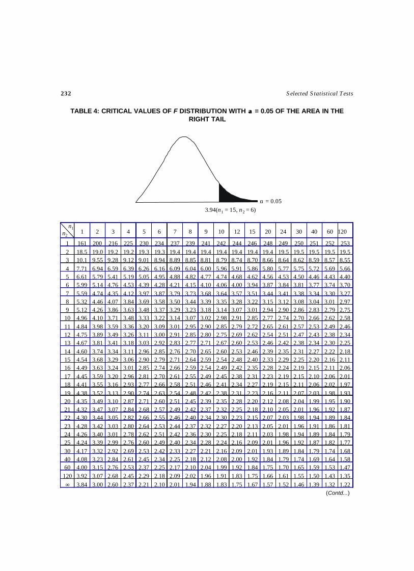
232 Selected Statistical Tests
TABLE 4: CRITICAL VALUES OF F DISTRIBUTION WITH αα = 0.05 OF THE AREA IN THERIGHT TAIL
1 2 3 4 5 6 7 8 9 10 12 15 20 24 30 40 60 120
1 161 200 216 225 230 234 237 239 241 242 244 246 248 249 250 251 252 253 2 18.5 19.0 19.2 19.2 19.3 19.3 19.4 19.4 19.4 19.4 19.4 19.4 19.4 19.5 19.5 19.5 19.5 19.5 3 10.1 9.55 9.28 9.12 9.01 8.94 8.89 8.85 8.81 8.79 8.74 8.70 8.66 8.64 8.62 8.59 8.57 8.55 4 7.71 6.94 6.59 6.39 6.26 6.16 6.09 6.04 6.00 5.96 5.91 5.86 5.80 5.77 5.75 5.72 5.69 5.66 5 6.61 5.79 5.41 5.19 5.05 4.95 4.88 4.82 4.77 4.74 4.68 4.62 4.56 4.53 4.50 4.46 4.43 4.40 6 5.99 5.14 4.76 4.53 4.39 4.28 4.21 4.15 4.10 4.06 4.00 3.94 3.87 3.84 3.81 3.77 3.74 3.70 7 5.59 4.74 4.35 4.12 3.97 3.87 3.79 3.73 3.68 3.64 3.57 3.51 3.44 3.41 3.38 3.34 3.30 3.27 8 5.32 4.46 4.07 3.84 3.69 3.58 3.50 3.44 3.39 3.35 3.28 3.22 3.15 3.12 3.08 3.04 3.01 2.97 9 5.12 4.26 3.86 3.63 3.48 3.37 3.29 3.23 3.18 3.14 3.07 3.01 2.94 2.90 2.86 2.83 2.79 2.75 10 4.96 4.10 3.71 3.48 3.33 3.22 3.14 3.07 3.02 2.98 2.91 2.85 2.77 2.74 2.70 2.66 2.62 2.58 11 4.84 3.98 3.59 3.36 3.20 3.09 3.01 2.95 2.90 2.85 2.79 2.72 2.65 2.61 2.57 2.53 2.49 2.46 12 4.75 3.89 3.49 3.26 3.11 3.00 2.91 2.85 2.80 2.75 2.69 2.62 2.54 2.51 2.47 2.43 2.38 2.34 13 4.67 3.81 3.41 3.18 3.03 2.92 2.83 2.77 2.71 2.67 2.60 2.53 2.46 2.42 2.38 2.34 2.30 2.25 14 4.60 3.74 3.34 3.11 2.96 2.85 2.76 2.70 2.65 2.60 2.53 2.46 2.39 2.35 2.31 2.27 2.22 2.18 15 4.54 3.68 3.29 3.06 2.90 2.79 2.71 2.64 2.59 2.54 2.48 2.40 2.33 2.29 2.25 2.20 2.16 2.11 16 4.49 3.63 3.24 3.01 2.85 2.74 2.66 2.59 2.54 2.49 2.42 2.35 2.28 2.24 2.19 2.15 2.11 2.06 17 4.45 3.59 3.20 2.96 2.81 2.70 2.61 2.55 2.49 2.45 2.38 2.31 2.23 2.19 2.15 2.10 2.06 2.01 18 4.41 3.55 3.16 2.93 2.77 2.66 2.58 2.51 2.46 2.41 2.34 2.27 2.19 2.15 2.11 2.06 2.02 1.97 19 4.38 3.52 3.13 2.90 2.74 2.63 2.54 2.48 2.42 2.38 2.31 2.23 2.16 2.11 2.07 2.03 1.98 1.93 20 4.35 3.49 3.10 2.87 2.71 2.60 2.51 2.45 2.39 2.35 2.28 2.20 2.12 2.08 2.04 1.99 1.95 1.90 21 4.32 3.47 3.07 2.84 2.68 2.57 2.49 2.42 2.37 2.32 2.25 2.18 2.10 2.05 2.01 1.96 1.92 1.87 22 4.30 3.44 3.05 2.82 2.66 2.55 2.46 2.40 2.34 2.30 2.23 2.15 2.07 2.03 1.98 1.94 1.89 1.84 23 4.28 3.42 3.03 2.80 2.64 2.53 2.44 2.37 2.32 2.27 2.20 2.13 2.05 2.01 1.96 1.91 1.86 1.81 24 4.26 3.40 3.01 2.78 2.62 2.51 2.42 2.36 2.30 2.25 2.18 2.11 2.03 1.98 1.94 1.89 1.84 1.79 25 4.24 3.39 2.99 2.76 2.60 2.49 2.40 2.34 2.28 2.24 2.16 2.09 2.01 1.96 1.92 1.87 1.82 1.77 30 4.17 3.32 2.92 2.69 2.53 2.42 2.33 2.27 2.21 2.16 2.09 2.01 1.93 1.89 1.84 1.79 1.74 1.68 40 4.08 3.23 2.84 2.61 2.45 2.34 2.25 2.18 2.12 2.08 2.00 1.92 1.84 1.79 1.74 1.69 1.64 1.58 60 4.00 3.15 2.76 2.53 2.37 2.25 2.17 2.10 2.04 1.99 1.92 1.84 1.75 1.70 1.65 1.59 1.53 1.47 120 3.92 3.07 2.68 2.45 2.29 2.18 2.09 2.02 1.96 1.91 1.83 1.75 1.66 1.61 1.55 1.50 1.43 1.35 ∞ 3.84 3.00 2.60 2.37 2.21 2.10 2.01 1.94 1.88 1.83 1.75 1.67 1.57 1.52 1.46 1.39 1.32 1.22
n1n2
3.94(n1 = 15, n2 = 6)α = 0.05
(Contd...)
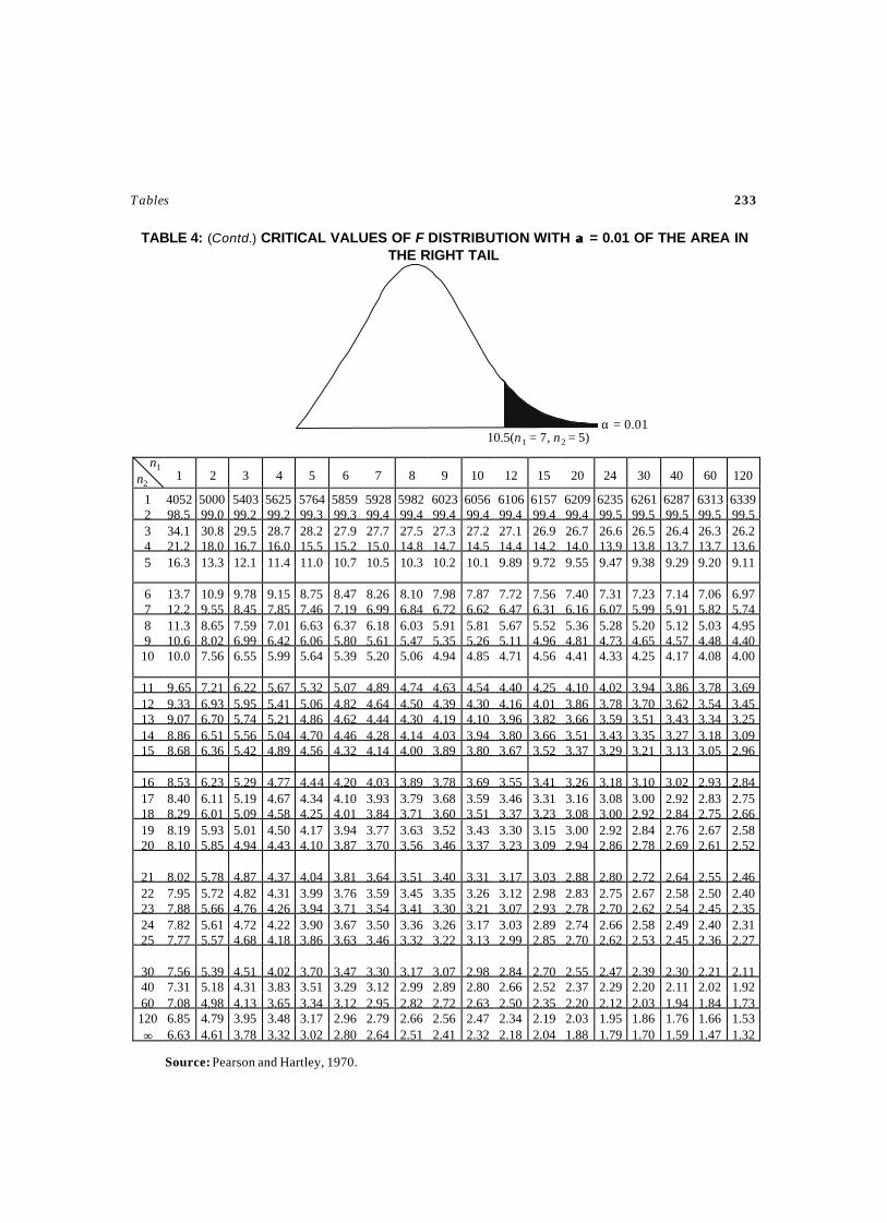
Tables 233
α = 0.0110.5(n1 = 7, n2 = 5)
n1
n2
1 2 3 4 5 6 7 8 9 10 12 15 20 24 30 40 60 120
1 4052 5000 5403 5625 5764 5859 5928 5982 6023 6056 6106 6157 6209 6235 6261 6287 6313 6339 2 98.5 99.0 99.2 99.2 99.3 99.3 99.4 99.4 99.4 99.4 99.4 99.4 99.4 99.5 99.5 99.5 99.5 99.5 3 34.1 30.8 29.5 28.7 28.2 27.9 27.7 27.5 27.3 27.2 27.1 26.9 26.7 26.6 26.5 26.4 26.3 26.2 4 21.2 18.0 16.7 16.0 15.5 15.2 15.0 14.8 14.7 14.5 14.4 14.2 14.0 13.9 13.8 13.7 13.7 13.6 5 16.3 13.3 12.1 11.4 11.0 10.7 10.5 10.3 10.2 10.1 9.89 9.72 9.55 9.47 9.38 9.29 9.20 9.11 6 13.7 10.9 9.78 9.15 8.75 8.47 8.26 8.10 7.98 7.87 7.72 7.56 7.40 7.31 7.23 7.14 7.06 6.97 7 12.2 9.55 8.45 7.85 7.46 7.19 6.99 6.84 6.72 6.62 6.47 6.31 6.16 6.07 5.99 5.91 5.82 5.74 8 11.3 8.65 7.59 7.01 6.63 6.37 6.18 6.03 5.91 5.81 5.67 5.52 5.36 5.28 5.20 5.12 5.03 4.95 9 10.6 8.02 6.99 6.42 6.06 5.80 5.61 5.47 5.35 5.26 5.11 4.96 4.81 4.73 4.65 4.57 4.48 4.40 10 10.0 7.56 6.55 5.99 5.64 5.39 5.20 5.06 4.94 4.85 4.71 4.56 4.41 4.33 4.25 4.17 4.08 4.00
11 9.65 7.21 6.22 5.67 5.32 5.07 4.89 4.74 4.63 4.54 4.40 4.25 4.10 4.02 3.94 3.86 3.78 3.69 12 9.33 6.93 5.95 5.41 5.06 4.82 4.64 4.50 4.39 4.30 4.16 4.01 3.86 3.78 3.70 3.62 3.54 3.45 13 9.07 6.70 5.74 5.21 4.86 4.62 4.44 4.30 4.19 4.10 3.96 3.82 3.66 3.59 3.51 3.43 3.34 3.25 14 8.86 6.51 5.56 5.04 4.70 4.46 4.28 4.14 4.03 3.94 3.80 3.66 3.51 3.43 3.35 3.27 3.18 3.09 15 8.68 6.36 5.42 4.89 4.56 4.32 4.14 4.00 3.89 3.80 3.67 3.52 3.37 3.29 3.21 3.13 3.05 2.96
16 8.53 6.23 5.29 4.77 4.44 4.20 4.03 3.89 3.78 3.69 3.55 3.41 3.26 3.18 3.10 3.02 2.93 2.84 17 8.40 6.11 5.19 4.67 4.34 4.10 3.93 3.79 3.68 3.59 3.46 3.31 3.16 3.08 3.00 2.92 2.83 2.75 18 8.29 6.01 5.09 4.58 4.25 4.01 3.84 3.71 3.60 3.51 3.37 3.23 3.08 3.00 2.92 2.84 2.75 2.66 19 8.19 5.93 5.01 4.50 4.17 3.94 3.77 3.63 3.52 3.43 3.30 3.15 3.00 2.92 2.84 2.76 2.67 2.58 20 8.10 5.85 4.94 4.43 4.10 3.87 3.70 3.56 3.46 3.37 3.23 3.09 2.94 2.86 2.78 2.69 2.61 2.52
21 8.02 5.78 4.87 4.37 4.04 3.81 3.64 3.51 3.40 3.31 3.17 3.03 2.88 2.80 2.72 2.64 2.55 2.46 22 7.95 5.72 4.82 4.31 3.99 3.76 3.59 3.45 3.35 3.26 3.12 2.98 2.83 2.75 2.67 2.58 2.50 2.40 23 7.88 5.66 4.76 4.26 3.94 3.71 3.54 3.41 3.30 3.21 3.07 2.93 2.78 2.70 2.62 2.54 2.45 2.35 24 7.82 5.61 4.72 4.22 3.90 3.67 3.50 3.36 3.26 3.17 3.03 2.89 2.74 2.66 2.58 2.49 2.40 2.31 25 7.77 5.57 4.68 4.18 3.86 3.63 3.46 3.32 3.22 3.13 2.99 2.85 2.70 2.62 2.53 2.45 2.36 2.27
30 7.56 5.39 4.51 4.02 3.70 3.47 3.30 3.17 3.07 2.98 2.84 2.70 2.55 2.47 2.39 2.30 2.21 2.11 40 7.31 5.18 4.31 3.83 3.51 3.29 3.12 2.99 2.89 2.80 2.66 2.52 2.37 2.29 2.20 2.11 2.02 1.92 60 7.08 4.98 4.13 3.65 3.34 3.12 2.95 2.82 2.72 2.63 2.50 2.35 2.20 2.12 2.03 1.94 1.84 1.73 120 6.85 4.79 3.95 3.48 3.17 2.96 2.79 2.66 2.56 2.47 2.34 2.19 2.03 1.95 1.86 1.76 1.66 1.53 ∞ 6.63 4.61 3.78 3.32 3.02 2.80 2.64 2.51 2.41 2.32 2.18 2.04 1.88 1.79 1.70 1.59 1.47 1.32
TABLE 4: (Contd.) CRITICAL VALUES OF F DISTRIBUTION WITH αα = 0.01 OF THE AREA INTHE RIGHT TAIL
Source: Pearson and Hartley, 1970.
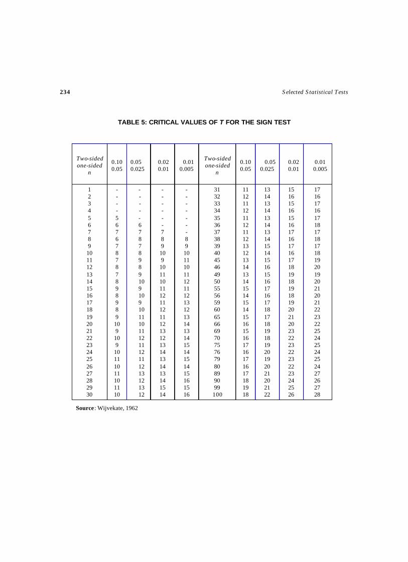
234 Selected Statistical Tests
TABLE 5: CRITICAL VALUES OF T FOR THE SIGN TEST
Two-sided one-sided
n
0.10 0.05
0.05 0.025
0.02 0.01
0.01 0.005
Two-sided one-sided
n
0.10 0.05
0.05 0.025
0.02 0.01
0.01 0.005
1 2 3 4 5 6 7 8 9 10 11 12 13 14 15 16 17 18 19 20 21 22 23 24 25 26 27 28 29 30
- - - - 5 6 7 6 7 8 7 8 7 8 9 8 9 8 9 10 9 10 9 10 11 10 11 10 11 10
- - - - - 6 7 8 7 8 9 8 9 109 109 10111011121112111213121312
- - - - - - 7 8 9 10 9 10 11 10 11 12 11 12 11 12 13 12 13 14 13 14 13 14 15 14
- - - - - - - 8 9 10 11 10 11 12 11 12 13 12 13 14 13 14 15 14 15 14 15 16 15 16
31 32 33 34 35 36 37 38 39 40 45 46 49 50 55 56 59 60 65 66 69 70 75 76 79 80 89 90 99 100
11 12 11 12 11 12 11 12 13 12 13 14 13 14 15 14 15 14 15 16 15 16 17 16 17 16 17 18 19 18
13 14 13 14 13 14 13 14 15 14 15 16 15 16 17 16 17 18 17 18 19 18 19 20 19 20 21 20 21 22
15 16 15 16 15 16 17 16 17 16 17 18 19 18 19 18 19 20 21 20 23 22 23 22 23 22 23 24 25 26
17 16 17 16 17 18 17 18 17 18 19 20 19 20 21 20 21 22 23 22 25 24 25 24 25 24 27 26 27 28
Source : Wijvekate, 1962
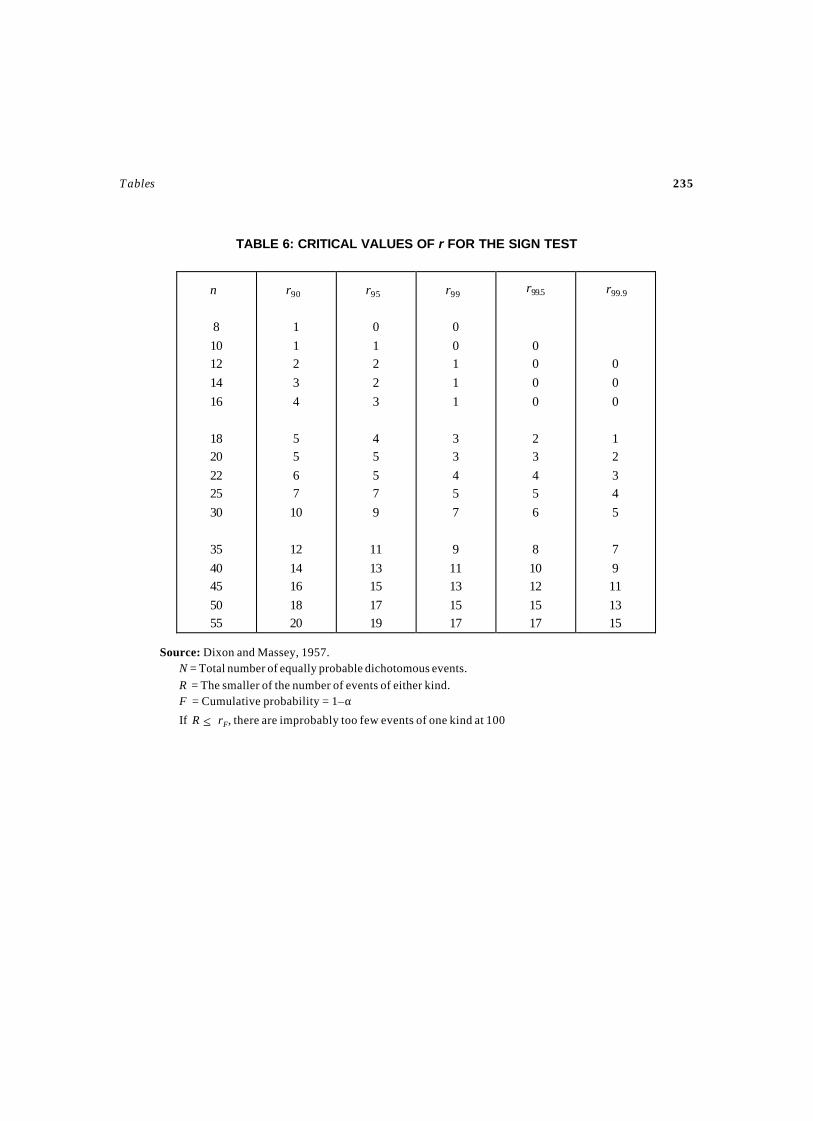
Tables 235
Source: Dixon and Massey, 1957.N = Total number of equally probable dichotomous events.R = The smaller of the number of events of either kind.F = Cumulative probability = 1– α
If R ≤ rF, there are improbably too few events of one kind at 100
TABLE 6: CRITICAL VALUES OF r FOR THE SIGN TEST
8
10 12
14
16
18 20
22 25
30
35
40 45
50 55
1
1 2
3
4
5 5
6 7
10
12
14 16
18 20
0
1 2
2
3
4 5
5 7
9
11
13 15
17 19
0
0 1
1
1
3 3
4 5
7
9
11 13
15 17
0 0
0
0
2 3
4 5
6
8
10 12
15 17
0
0
0
1 2
3 4
5
7
9 11
13 15
n r90 r95 r99 r99.5 r99.9
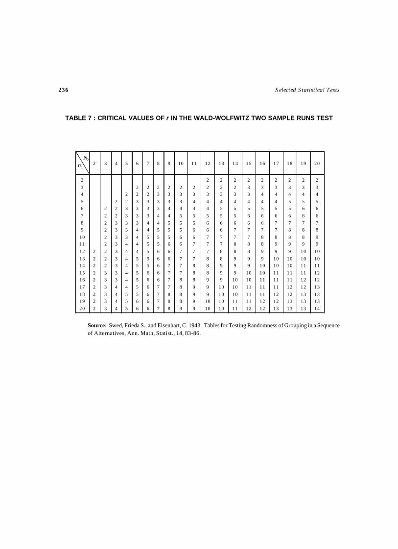
236 Selected Statistical Tests
TABLE 7 : CRITICAL VALUES OF r IN THE WALD-WOLFWITZ TWO SAMPLE RUNS TEST
2 3 4
5
6
7
8
9
10
1 1
12 13
1 4
15 16
1 7
18 19
20
2
3 4
5 6
7
8 9
10 11
12
13 14
15 16
17
18 19
20
2
2 2
2 2
2
2 2
2
2
2
2 2
2 2
2
2 2
3 3
3
3 3
3
2 2
2
3 3
3 3
3
3 3
3 3
4
4 4
4
2
2 3
3
3 3
3 4
4
4 4
4 4
4
5 5
5
2 2
3 3
3
3 4
4 4
4
5 5
5 5
5
5 6
6
2 2
3 3
3
4 4
5 5
5
5 5
6 6
6
6 6
6
2 3
3 3
4
4 5
5 5
6
6 6
6 6
7
7 7
7
2 3
3 4
4
5 5
5 6
6
6 7
7 7
7
8 8
8
2 3
3 4
5
5 5
6 6
7
7 7
7 8
8
8 8
9
2 3
4 4
5
5 6
6 7
7
7 8
8 8
9
9 9
9
2
2 3
4 4
5
6 6
7 7
7
8 8
8 9
9
9 10
10
2
2 3
4 5
5
6 6
7 7
8
8 9
9 9
10
10 10
10
2
2 3
4 5
5
6 7
7 8
8
9 9
9 10
10
10 11
11
2
3 3
4 5
6
6 7
7 8
8
9 9
10 10
11
11 11
12
2
3 4
4 5
6
6 7
8 8
9
9 10
10 11
11
11 12
12
2
3 4
4 5
6
7 7
8 9
9
10 10
11 11
11
12 12
13
2
3 4
5 5
6
7 8
8 9
9
10 10
11 11
12
12 13
13
2
3 4
5 6
6
7 8
8 9
10
10 11
11 12
12
13 13
13
2
3 4
5 6
6
7 8
9 9
10
10 11
12 12
13
13 13
14
Source: Swed, Frieda S., and Eisenhart, C. 1943. Tables for Testing Randomness of Grouping in a Sequenceof Alternatives, Ann. Math, Statist., 14, 83-86.
N2
n1

Tables 237
TABLE 8: CRITICAL VALUES OF THE SMALLEST RANK SUM FOR THE WILCOXON-MANN-WHITNEY TEST
n1 n2
3 2 3 – – –
3 3 7 6 – –
4 2 3 – – –
4 3 7 6 – –
4 4 13 11 10 –
5 2 4 3 – –
5 3 8 7 6 –5 4 14 12 11 –5 5 20 19 17 15
6 2 4 3 – –6 3 9 8 7 –6 4 15 13 12 106 5 22 20 18 16
6 6 30 28 26 13
7 2 4 3 – –
7 3 10 8 7 –
7 4 16 14 13 107 5 23 21 20 167 6 32 29 27 24
7 7 41 39 36 328 2 5 4 3 –8 3 11 9 8 –8 4 17 15 14 11
8 5 25 2 21 178 6 34 31 29 258 7 44 41 38 348 8 55 51 49 43
9 1 1 – – –9 2 5 4 3 –9 3 11 9 8 6
9 4 19 16 14 11
9 5 27 24 22 18
9 6 36 33 31 26
(Contd...)
Two-sided
one-sided0.10 0.05 0.02 0.01
0.05 0.025 0.01 0.005
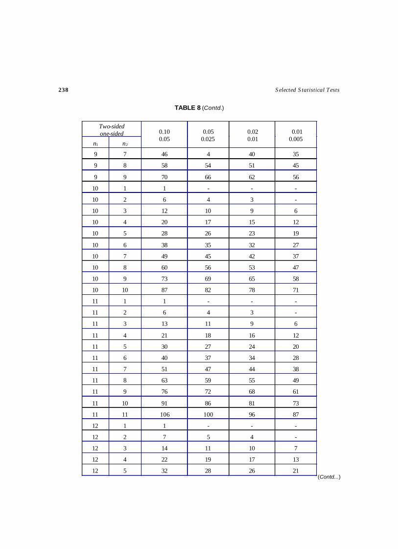
238 Selected Statistical Tests
TABLE 8 (Contd.)
Two-sided one-sided
n1 n2
0.10 0.05
0.05 0.025
0.02 0.01
0.01 0.005
9 7 46 4 40 35
9 8 58 54 51 45
9 9 70 66 62 56
10 1 1 - - -
10 2 6 4 3 -
10 3 12 10 9 6
10 4 20 17 15 12
10 5 28 26 23 19
10 6 38 35 32 27
10 7 49 45 42 37
10 8 60 56 53 47
10 9 73 69 65 58
10 10 87 82 78 71
11 1 1 - - -
11 2 6 4 3 -
11 3 13 11 9 6
11 4 21 18 16 12
11 5 30 27 24 20
11 6 40 37 34 28
11 7 51 47 44 38
11 8 63 59 55 49
11 9 76 72 68 61
11 10 91 86 81 73
11 11 106 100 96 87
12 1 1 - - -
12 2 7 5 4 -
12 3 14 11 10 7
12 4 22 19 17 13
12 5 32 28 26 21
(Contd...)
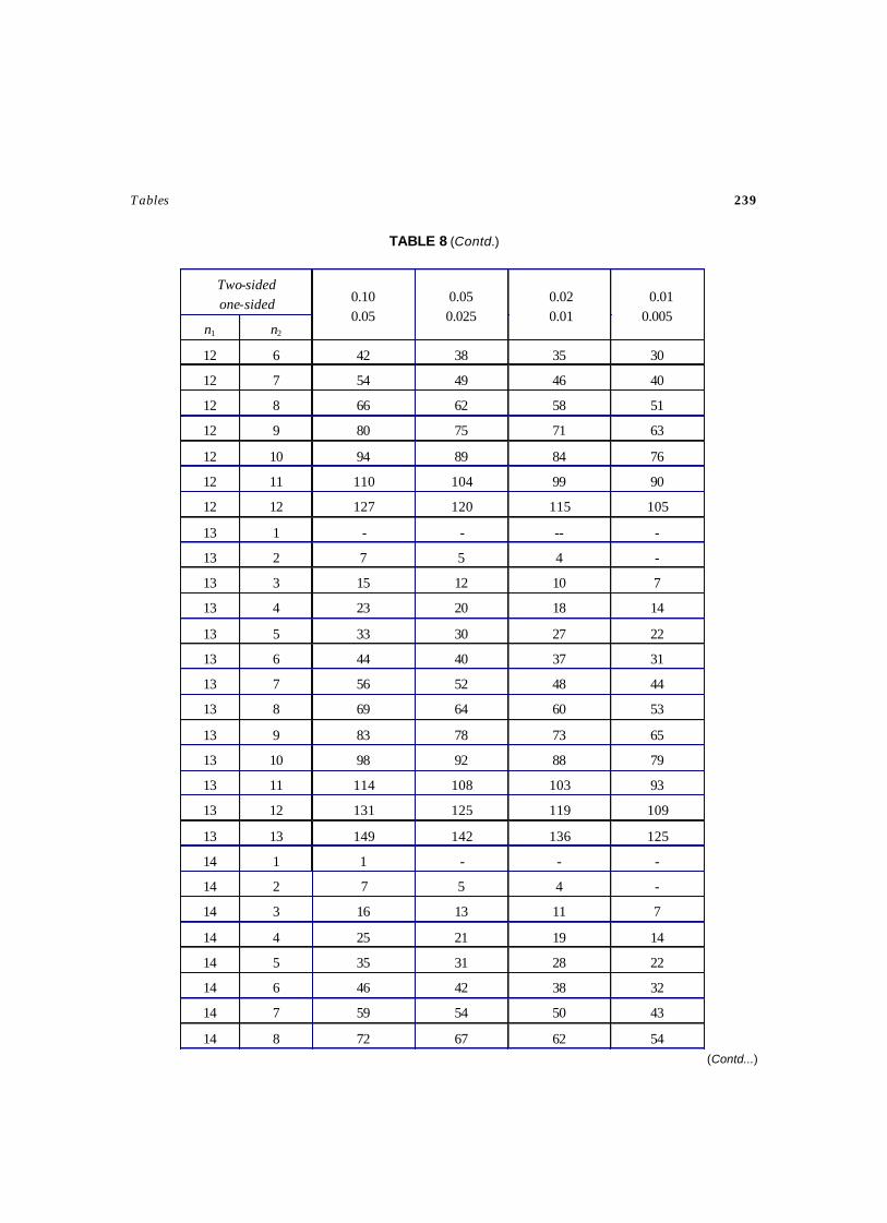
Tables 239
Two-sided one-sided
n1 n2
0.10 0.05
0.05 0.025
0.02 0.01
0.01 0.005
12 6 42 38 35 30
12 7 54 49 46 40
12 8 66 62 58 51
12 9 80 75 71 63
12 10 94 89 84 76
12 11 110 104 99 90
12 12 127 120 115 105
13 1 - - -- -
13 2 7 5 4 -
13 3 15 12 10 7
13 4 23 20 18 14
13 5 33 30 27 22
13 6 44 40 37 31
13 7 56 52 48 44
13 8 69 64 60 53
13 9 83 78 73 65
13 10 98 92 88 79
13 11 114 108 103 93
13 12 131 125 119 109
13 13 149 142 136 125
14 1 1 - - -
14 2 7 5 4 -
14 3 16 13 11 7
14 4 25 21 19 14
14 5 35 31 28 22
14 6 46 42 38 32
14 7 59 54 50 43
14 8 72 67 62 54
TABLE 8 (Contd.)
(Contd...)
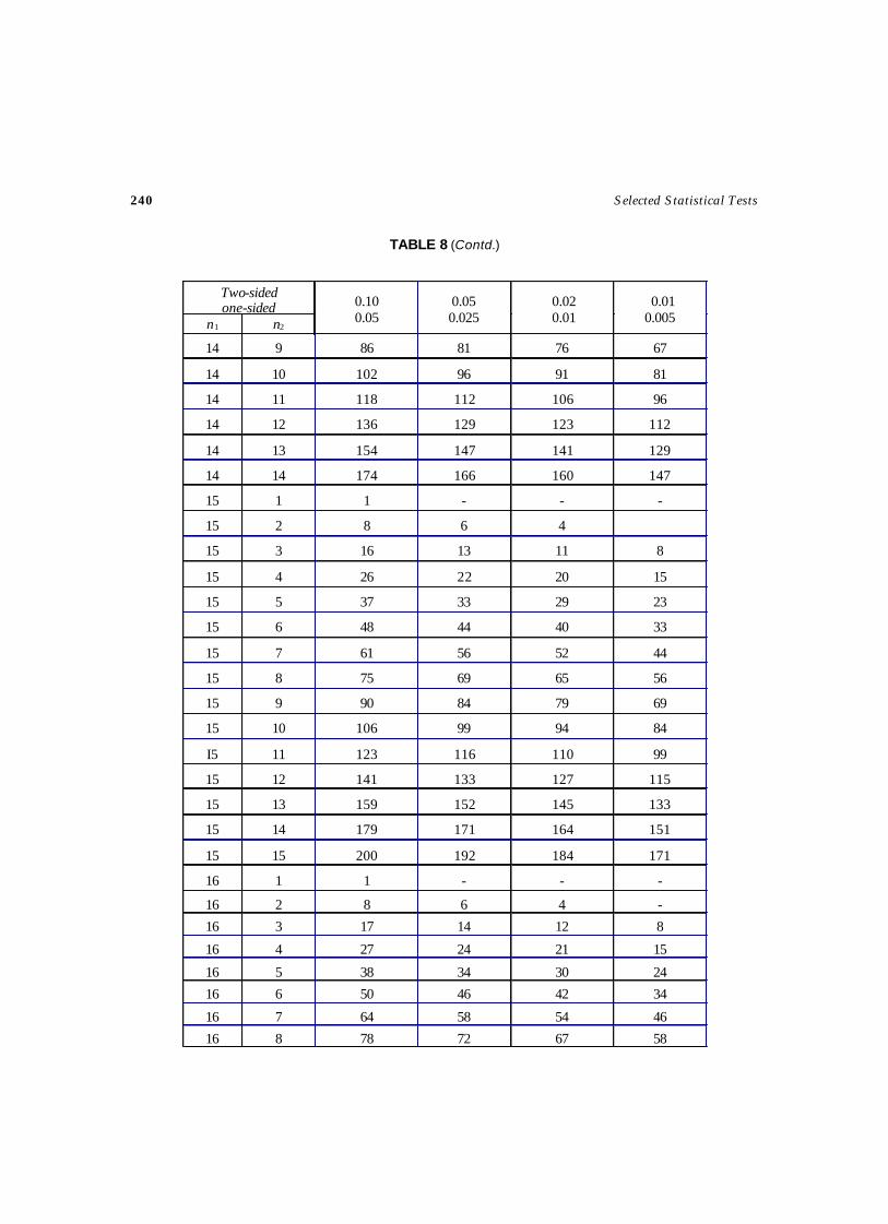
240 Selected Statistical Tests
TABLE 8 (Contd.)
Two-sided one-sided
n1 n2
0.10 0.05
0.05 0.025
0.02 0.01
0.01 0.005
14 9 86 81 76 67
14 10 102 96 91 81
14 11 118 112 106 96
14 12 136 129 123 112
14 13 154 147 141 129
14 14 174 166 160 147
15 1 1 - - -
15 2 8 6 4
15 3 16 13 11 8
15 4 26 22 20 15
15 5 37 33 29 23
15 6 48 44 40 33
15 7 61 56 52 44
15 8 75 69 65 56
15 9 90 84 79 69
15 10 106 99 94 84
I5 11 123 116 110 99
15 12 141 133 127 115
15 13 159 152 145 133
15 14 179 171 164 151
15 15 200 192 184 171
16 1 1 - - -
16 2 8 6 4 -
16 3 17 14 12 8
16 4 27 24 21 15
16 5 38 34 30 24
16 6 50 46 42 34
16 7 64 58 54 46
16 8 78 72 67 58
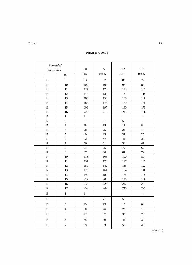
Tables 241
TABLE 8 (Contd.)
n1 n2
16 9 93 87 82 72
16 10 109 103 97 86
16 11 127 120 113 102
16 12 145 138 131 119
16 13 165 156 150 130
16 14 185 176 169 155
16 15 206 197 190 175
16 16 229 219 211 196
17 1 1 – – –
17 2 9 6 5 –
17 3 18 15 12 8
17 4 28 25 21 16
17 5 40 35 32 25
17 6 52 47 43 36
17 7 66 61 56 47
17 8 81 75 70 60
17 9 97 90 84 74
17 10 113 106 100 89
17 11 131 123 117 105
17 12 150 142 135 122
17 13 170 161 154 140
17 14 190 182 174 159
17 15 212 203 195 180
17 16 235 225 217 201
17 17 259 249 240 223
18 1 1 – – –
18 2 9 7 5
18 3 19 15 13 8
18 4 30 26 22 16
18 5 42 37 33 26
18 6 55 49 45 37
18 7 69 63 58 49
(Contd...)
Two-sided
one-sided 0.10 0.05 0.02 0.01
0.05 0.025 0.01 0.005
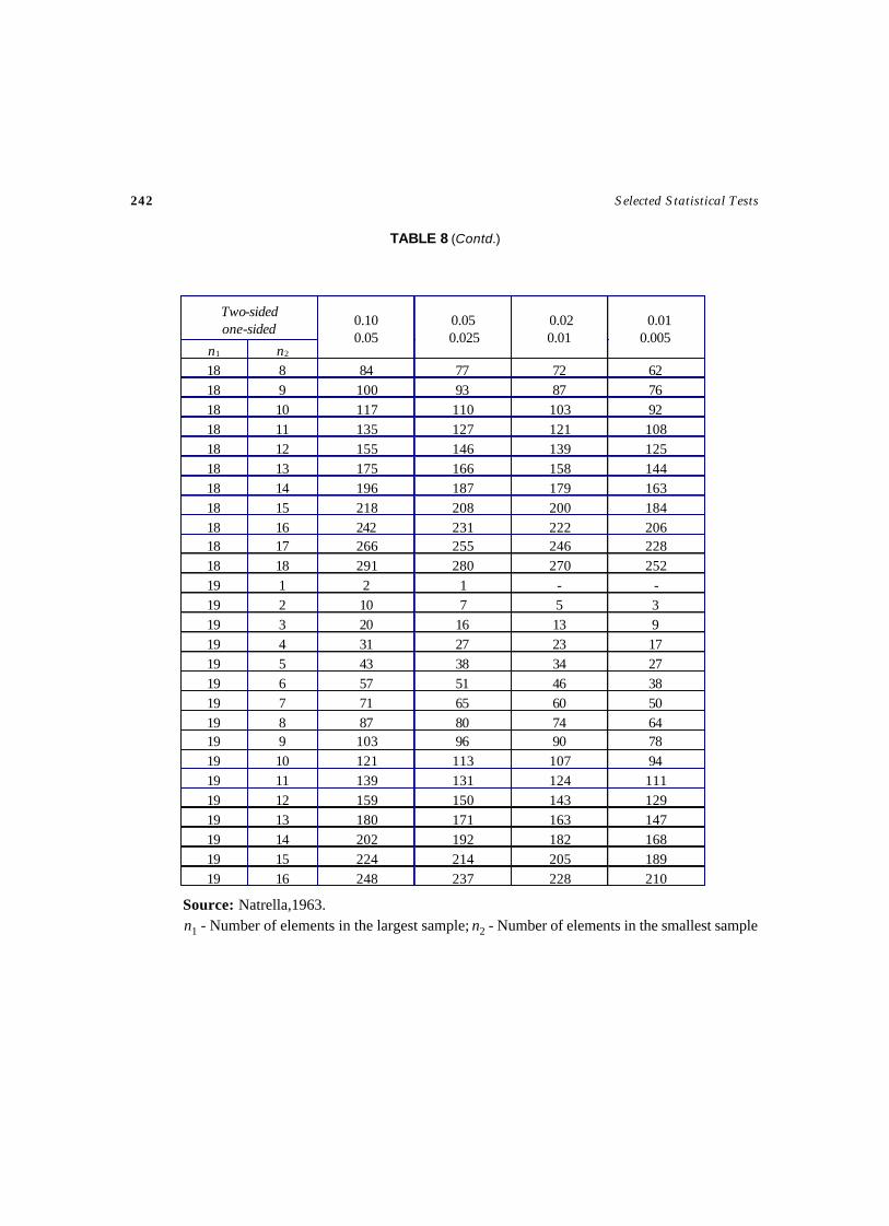
242 Selected Statistical Tests
TABLE 8 (Contd.)
Source: Natrella,1963. n1 - Number of elements in the largest sample; n2 - Number of elements in the smallest sample
Two-sided one-sided
n1 n2
0.10 0.05
0.05 0.025
0.02 0.01
0.01 0.005
18 8 84 77 72 62 18 9 100 93 87 76 18 10 117 110 103 92 18 11 135 127 121 108 18 12 155 146 139 125 18 13 175 166 158 144 18 14 196 187 179 163 18 15 218 208 200 184 18 16 242 231 222 206 18 17 266 255 246 228 18 18 291 280 270 252 19 1 2 1 - - 19 2 10 7 5 3 19 3 20 16 13 9 19 4 31 27 23 17 19 5 43 38 34 27 19 6 57 51 46 38 19 7 71 65 60 50 19 8 87 80 74 64 19 9 103 96 90 78 19 10 121 113 107 94 19 11 139 131 124 111 19 12 159 150 143 129 19 13 180 171 163 147 19 14 202 192 182 168 19 15 224 214 205 189 19 16 248 237 228 210
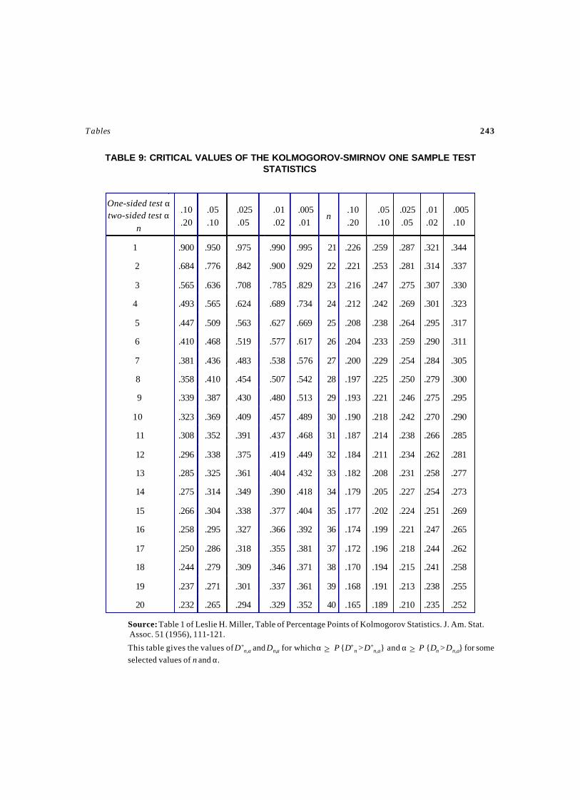
Tables 243
TABLE 9: CRITICAL VALUES OF THE KOLMOGOROV-SMIRNOV ONE SAMPLE TESTSTATISTICS
Source: Table 1 of Leslie H. Miller, Table of Percentage Points of Kolmogorov Statistics. J. Am. Stat. Assoc. 51 (1956), 111-121.
This table gives the values of D+n,a and Dn,a for which α ≥ P {D+
n > D+n,a} and α ≥ P {Dn > Dn,a} for some
selected values of n and α.
.10 .20
.05
.10 .025
.05 .01 .02
.005 .01
n .10 .20
.05
.10 .025 .05
.01
.02 .005 .10
1 .900 .950 .975 .990 .995 21 .226 .259 .287 .321 .344
2 .684 .776 .842 .900 .929 22 .221 .253 .281 .314 .337
3 .565 .636 .708 .785 .829 23 .216 .247 .275 .307 .330
4 .493 .565 .624 .689 .734 24 .212 .242 .269 .301 .323
5 .447 .509 .563 .627 .669 25 .208 .238 .264 .295 .317
6 .410 .468 .519 .577 .617 26 .204 .233 .259 .290 .311
7 .381 .436 .483 .538 .576 27 .200 .229 .254 .284 .305
8 .358 .410 .454 .507 .542 28 .197 .225 .250 .279 .300
9 .339 .387 .430 .480 .513 29 .193 .221 .246 .275 .295
10 .323 .369 .409 .457 .489 30 .190 .218 .242 .270 .290
11 .308 .352 .391 .437 .468 31 .187 .214 .238 .266 .285
12 .296 .338 .375 .419 .449 32 .184 .211 .234 .262 .281
13 .285 .325 .361 .404 .432 33 .182 .208 .231 .258 .277
14 .275 .314 .349 .390 .418 34 .179 .205 .227 .254 .273
15 .266 .304 .338 .377 .404 35 .177 .202 .224 .251 .269
16 .258 .295 .327 .366 .392 36 .174 .199 .221 .247 .265
17 .250 .286 .318 .355 .381 37 .172 .196 .218 .244 .262
18 .244 .279 .309 .346 .371 38 .170 .194 .215 .241 .258
19 .237 .271 .301 .337 .361 39 .168 .191 .213 .238 .255
20 .232 .265 .294 .329 .352 40 .165 .189 .210 .235 .252
One-sided test αtwo-sided test α
n
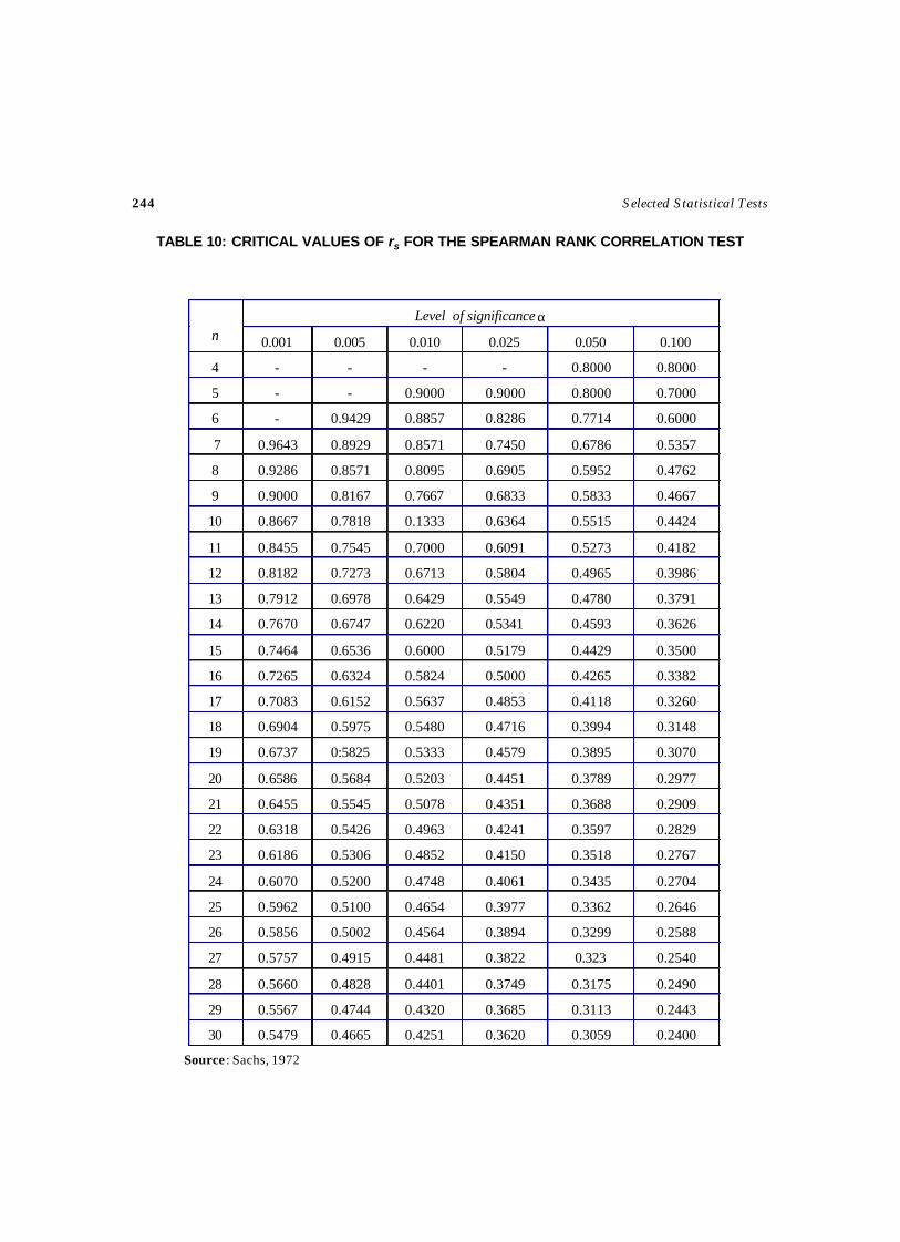
244 Selected Statistical Tests
TABLE 10: CRITICAL VALUES OF rs FOR THE SPEARMAN RANK CORRELATION TEST
Level of significance α n 0.001 0.005 0.010 0.025 0.050 0.100
4 - - - - 0.8000 0.8000
5 - - 0.9000 0.9000 0.8000 0.7000
6 - 0.9429 0.8857 0.8286 0.7714 0.6000
7 0.9643 0.8929 0.8571 0.7450 0.6786 0.5357
8 0.9286 0.8571 0.8095 0.6905 0.5952 0.4762
9 0.9000 0.8167 0.7667 0.6833 0.5833 0.4667
10 0.8667 0.7818 0.1333 0.6364 0.5515 0.4424
11 0.8455 0.7545 0.7000 0.6091 0.5273 0.4182
12 0.8182 0.7273 0.6713 0.5804 0.4965 0.3986
13 0.7912 0.6978 0.6429 0.5549 0.4780 0.3791
14 0.7670 0.6747 0.6220 0.5341 0.4593 0.3626
15 0.7464 0.6536 0.6000 0.5179 0.4429 0.3500
16 0.7265 0.6324 0.5824 0.5000 0.4265 0.3382
17 0.7083 0.6152 0.5637 0.4853 0.4118 0.3260
18 0.6904 0.5975 0.5480 0.4716 0.3994 0.3148
19 0.6737 0:5825 0.5333 0.4579 0.3895 0.3070
20 0.6586 0.5684 0.5203 0.4451 0.3789 0.2977
21 0.6455 0.5545 0.5078 0.4351 0.3688 0.2909
22 0.6318 0.5426 0.4963 0.4241 0.3597 0.2829
23 0.6186 0.5306 0.4852 0.4150 0.3518 0.2767
24 0.6070 0.5200 0.4748 0.4061 0.3435 0.2704
25 0.5962 0.5100 0.4654 0.3977 0.3362 0.2646
26 0.5856 0.5002 0.4564 0.3894 0.3299 0.2588
27 0.5757 0.4915 0.4481 0.3822 0.323 0.2540
28 0.5660 0.4828 0.4401 0.3749 0.3175 0.2490
29 0.5567 0.4744 0.4320 0.3685 0.3113 0.2443
30 0.5479 0.4665 0.4251 0.3620 0.3059 0.2400
Source : Sachs, 1972
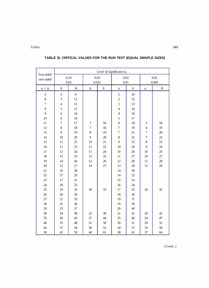
Tables 245
TABLE 11: CRITICAL VALUES FOR THE RUN TEST (EQUAL SMAPLE SIZES)
Level of significance α Two-sided
one-sided 0.10 0.05
0.05 0.025
0.02 0.01
0.01 0.005
n1 = n2 A B A b a b a B
5 6
7
8 9
10 11
12 13
14 15
16
17 18
19 20
21 22
23
24 25
26 27
28 29
30 35
40
45 50
3 3
4
5 6
6 7
8 9
10 11
11
12 13
14 15
16 17
17
18 19
20 21
22 23
24 28
33
37 42
9 11
12
13 14
16 17
18 19
20 21
23
24 25
26 27
28 29
31
32 33
34 35
36 37
38 43
48
54 59
7
7 8
9 10
11
11 12
13 14
18
22 27
31
36 40
16
18 19
20 21
22
24 25
26 27
33
39 44
50
55 61
2 2
3
4 4
5 6
7 7
8 9
10
10 11
12 13
14 14
15
16 17
18 19
19 20
21 25
30
34 38
10 12
13
14 16
17 18
19 21
22 23
24
26 27
28 29
30 32
33
34 35
36 37
39 40
41 46
51
57 63
5
6 7
7 8
9
10 10
11 12
16
20 24
29
33 37
18
19 20
22 23
24
25 27
28 29
35
41 47
52
58 64
(Contd.. .)
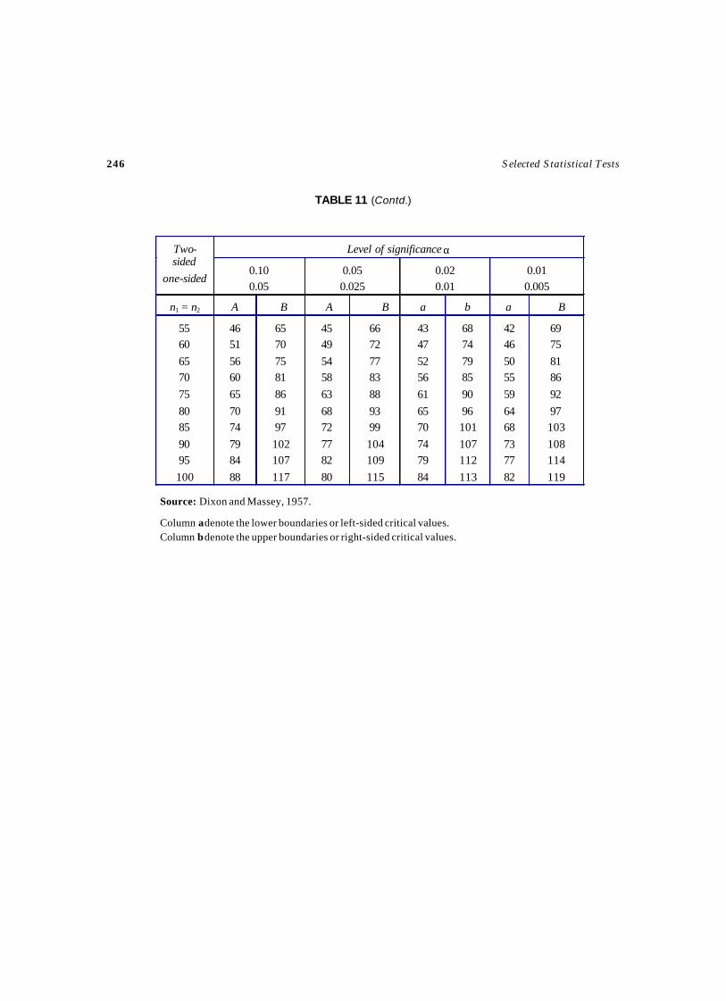
246 Selected Statistical Tests
Level of significance α Two-sided
one-sided 0.10 0.05
0.05 0.025
0.02 0.01
0.01 0.005
n1 = n2 A B A B a b a B
55 60
65 70
75
80 85
90 95
100
46 51
56 60
65
70 74
79 84
88
65 70
75 81
86
91 97
102 107
117
45 49
54 58
63
68 72
77 82
80
66 72
77 83
88
93 99
104 109
115
43 47
52 56
61
65 70
74 79
84
68 74
79 85
90
96 101
107 112
113
42 46
50 55
59
64 68
73 77
82
69 75
81 86
92
97 103
108 114
119
TABLE 11 (Contd.)
Source: Dixon and Massey, 1957.
Column a denote the lower boundaries or left-sided critical values.Column b denote the upper boundaries or right-sided critical values.
Anderson, T.W., (1974), An Introduction to Multivariate Statistical Analysis, Wiley Eastern,2nd edition, New Delhi.
Chakravarti, I.M., Laha, R.G. & Roy, J. (1967), Hand Book of Methods of Applied Statistics, Vol II,John Wiley.
Cochran, W.G. & Cox, G.M. (1959), Experimental Designs, Asia Publishing House.
Dixon, W.J. and Massey, F.J. (1957), Introduction to Statistical Analysis, McGraw-Hill, New York.
Fisher, R.A. (1947), The Design of Experiments, Oliver and Boyd.
Fisher, R.A. and Yates, F. (1974), Statistical Tables for Biological, Agricultural and MedicalResearch, 6th edn. Oliver and Boyd, Edinburgh.
Graybill, F.A. (1961), An Introduction to Linear Statistical Models, Vol.1, McGraw-Hill.
Gibbons, J.D. and Chakraborti, S. (1992), Non-parametric Statistical Inference, 5th ed., MarcelDekker, New York.
Gopal, K. Kanji, 100 Statistical Tests, SAGE Publications.
Goulden, C.H. (1959), Methods of Statistical Analysis, Asia Publishing House.
Gupta, S.C. and Kapoor, V.K. (2002), Fundamentals of Mathematical Statistics, Sultan Chand &Sons.
Gupta, S.C. and Kapoor, V.K. (1996), Fundamentals of Mathematical Statistics, Sultan Chand &Sons.
Hogg, R.V. and Craig, A.T. (1965), Introduction to Mathematical Statistics, Macmillan and Amerind.
Johnson, R.A. and Wichern, D.W. (1996), Applied Multivariate Statistical Analysis, 3rd ed., PrenticeHall of India, Pvt. Ltd.
Kempthorne, O. (1965), The Design and Analysis of Experiments, John Wiley & Sons.
Mood, A.M. Graybill, F.A. and Boes, D.C. (1974), An Introduction to the Theory of Statistics,McGraw-Hill and Tata McGraw-Hill.
Natrella, M.G. (1963), Experimental Statistics, National Bureau of Standards Handbook, 91, USGovernment Printing Office, Washington.
REFERENCES

248 Selected Statistical Tests
Parimal Mukhopadhyay (1996), Mathematical Statistics, New Central Book Agency (P) Ltd.,Calcutta.
Parimal Mukhopadhyay (1999), Applied Statistics, New Central Book Agency (P) Ltd, Calcutta.
Rangasamy, R. (1995), A Text Book of Agricultural Statistics, New Age International PublishersLtd.
Rao, C.R. (1963), Linear Statistical Inference and Its Applications, John Wiley & Sons.
Rao, C.R. (1952), Advanced Statistical Methods in Biometric Research, John Wiley & Sons.
Richard I. Levin and David S. Rubin (2001), Statistics for Management, 7th ed., Prentice Hall ofIndia.
Rohatgi, V.K. (1976), An Introduction to Probability Theory and Mathematical Statistics, WileyEatern.
Sachs, L. (1972), Statistische Methoden: ein Soforthelfer, Springer-Verlag, Berlin.
Scheffe, H. (1961), The Analysis of Variance, John Wiley & Sons, New York.
Searle, S.R. (1971), Linear Models, John Wiley & Sons, New York.
Wald, A. (1947), Sequential Analysis, John Wiley & Sons, New York.
Walpole, R.E. and Myers, R.H. (1989), Probability and Statistics for Engineers and Scientists, 4th
edn. Macmillan, New York.
Wijvekate, M.L. (1962), Verklarende Statistick, Aula, Utrecht.