Seismic Waveform Tomography

Jeroen Tromp

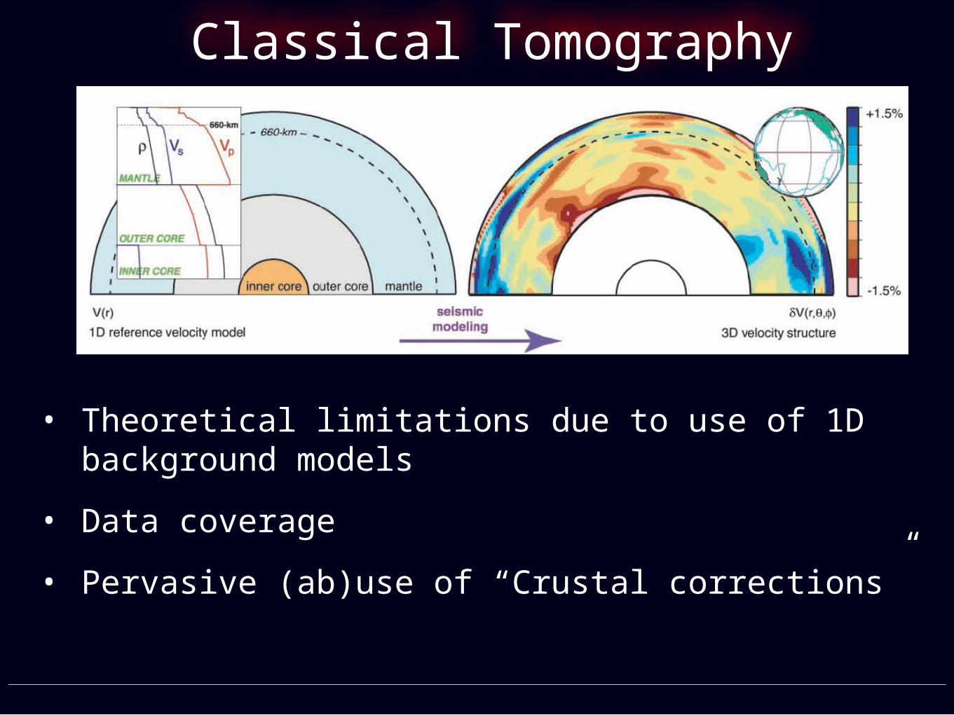
Classical Tomography

• Theoretical limitations due to use of 1D background models

• Data coverage

• Pervasive (ab)use of “Crustal corrections”

• We need abundant high-quality data

• We also need to harness the data that we already have

• The solution to gaps in data coverage is not only more data, but also using more of the data we already have

• This requires sophisticated forward and inverse modeling tools, data assimilation, and computational resources

A Marriage of Data and Simulation

Challenges in Seismic Tomography

• Theoretical limitations

- Finite-frequency effects have become important

P Wave: Finite-Frequency Effects

27 s 18 s

9 s

Challenges in Seismic Tomography

• Data coverage

- Uneven global distribution of earthquakes and stations

- Amount of usable data is determined by the accuracy of the forward method

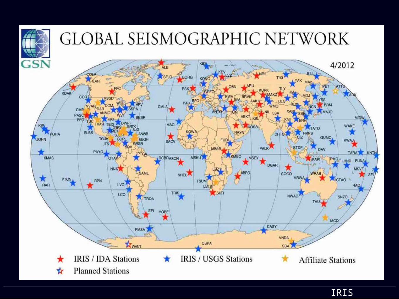
IRIS

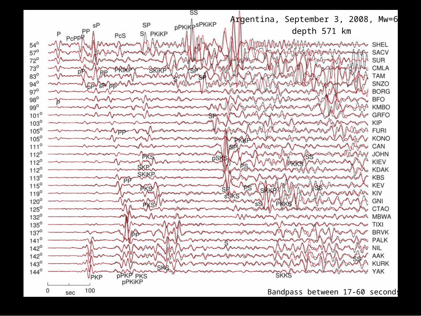
Argentina, September 3, 2008, Mw=6.3,depth 571 km

Bandpass between 17-60 seconds

Challenges in Seismic Tomography

• Crustal effects

- Can be highly nonlinear, thus “crustal corrections” are questionable

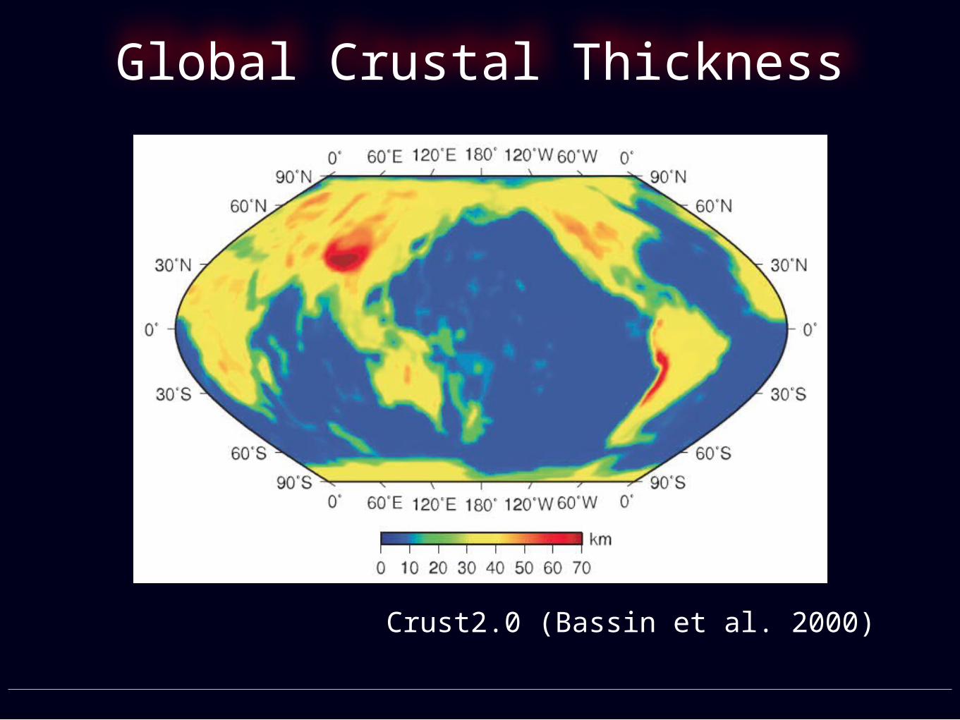
Global Crustal Thickness

Crust2.0 (Bassin et al. 2000)

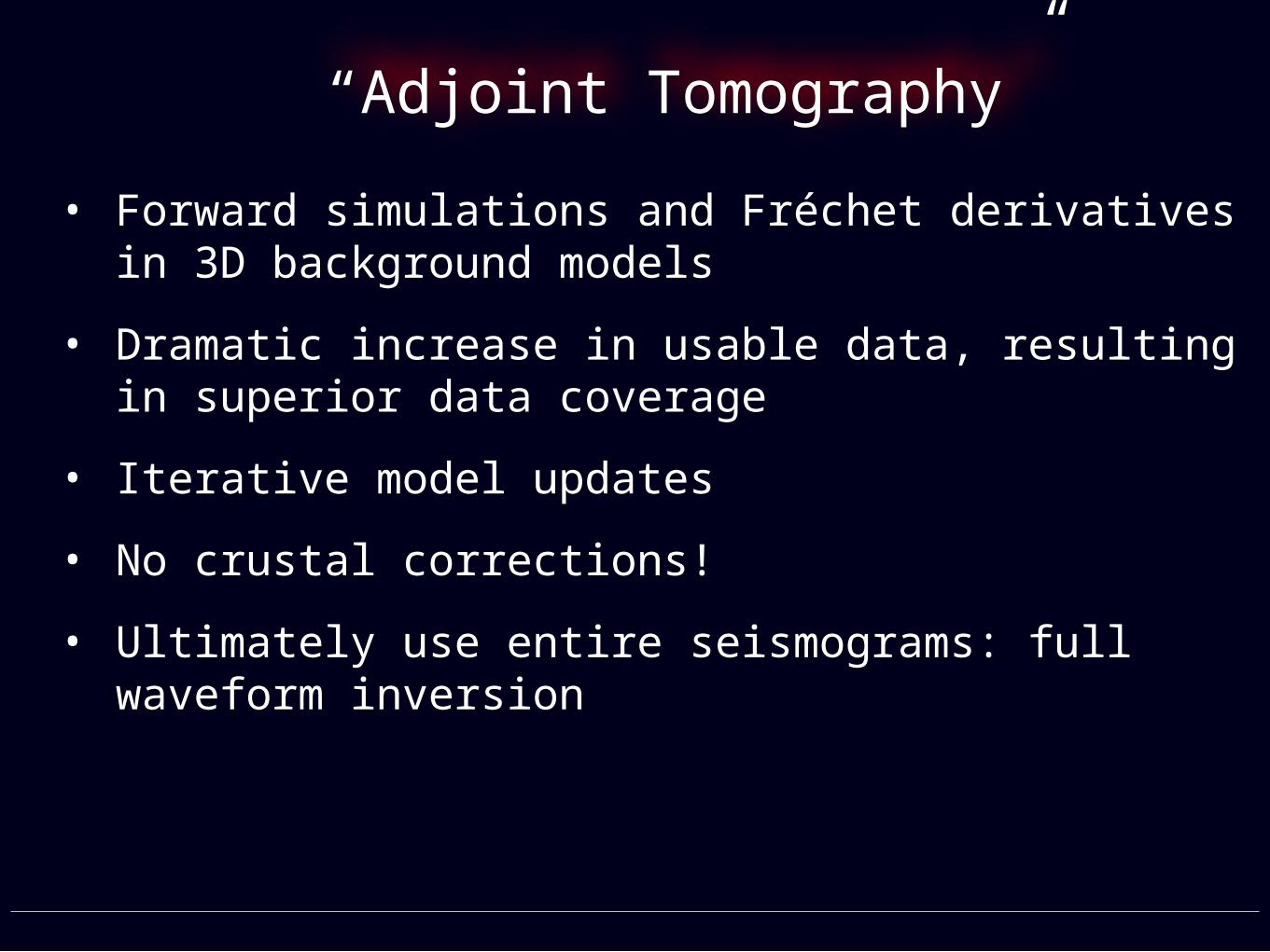
“Adjoint Tomography”

• Forward simulations and Fréchet derivatives in 3D background models

• Dramatic increase in usable data, resulting in superior data coverage

• Iterative model updates

• No crustal corrections!

• Ultimately use entire seismograms: full waveform inversion

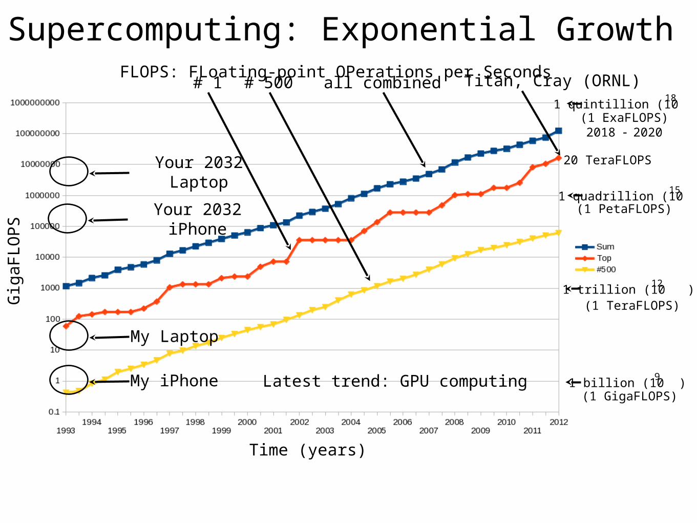
# 1 # 500 all combinedFLOPS: FLoating-point OPerations per Seconds

Latest trend: GPU computing

My Laptop

TOP500.org

Supercomputing: Exponential Growth

1 billion (10 )9

(1 GigaFLOPS)

1 trillion (10 )12

(1 TeraFLOPS)

1 quadrillion (10 )15

(1 PetaFLOPS)

181 quintillion (10 )

(1 ExaFLOPS)2018 - 2020

My iPhone

Titan, Cray (ORNL)

20 TeraFLOPSYour 2032 Laptop

Gig

aFL

OPS

Time (years)

Your 2032 iPhone

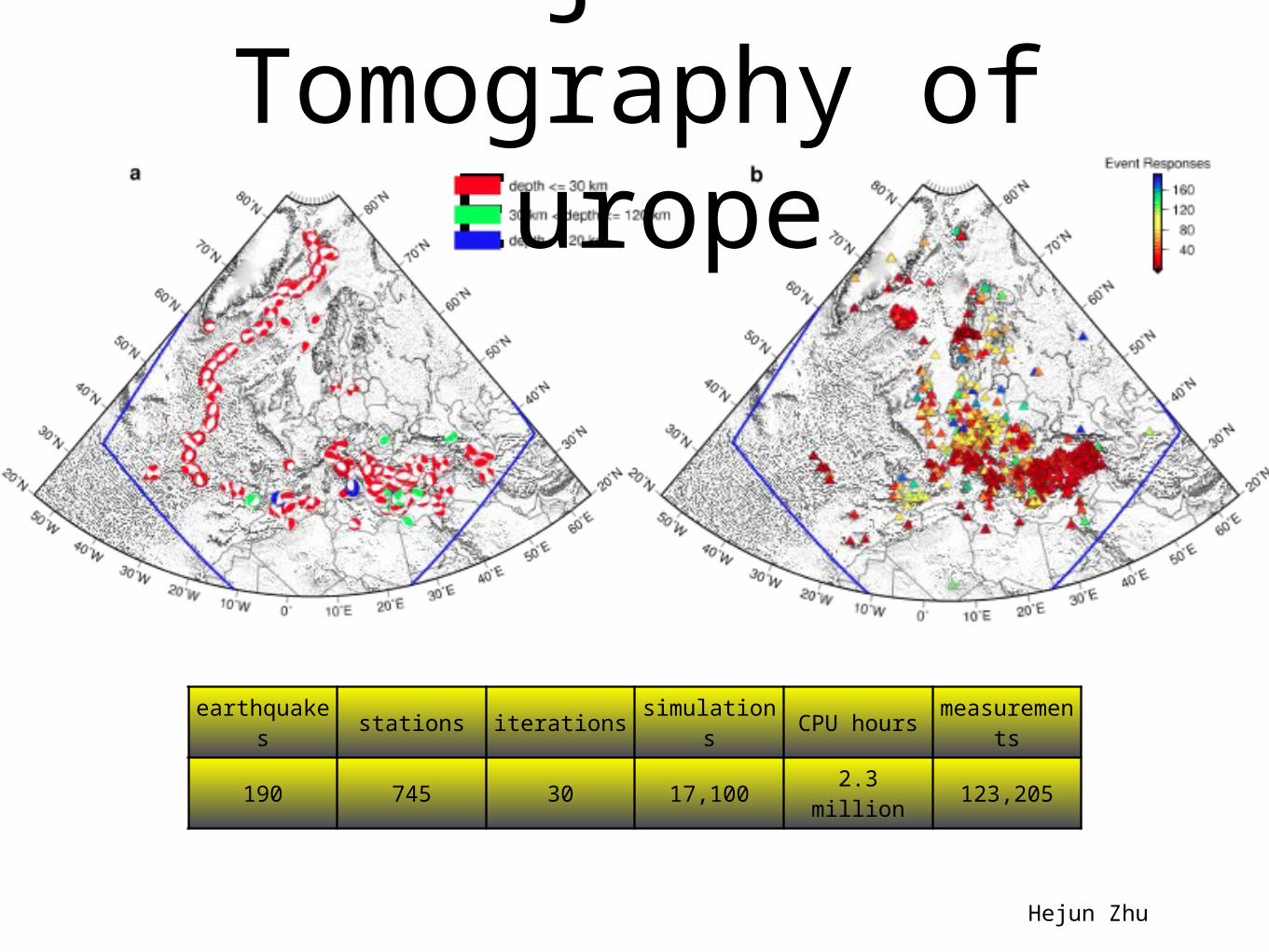
Adjoint Tomography of

Europe

earthquakes stations iterations simulations CPU hours measureme

nts

190 745 30 17,100 2.3 million 123,205

Hejun Zhu

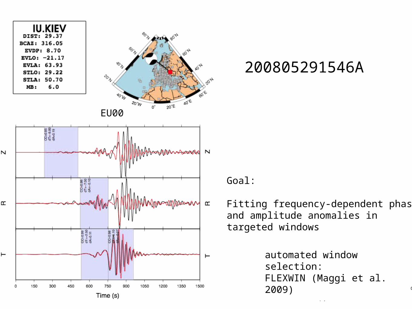
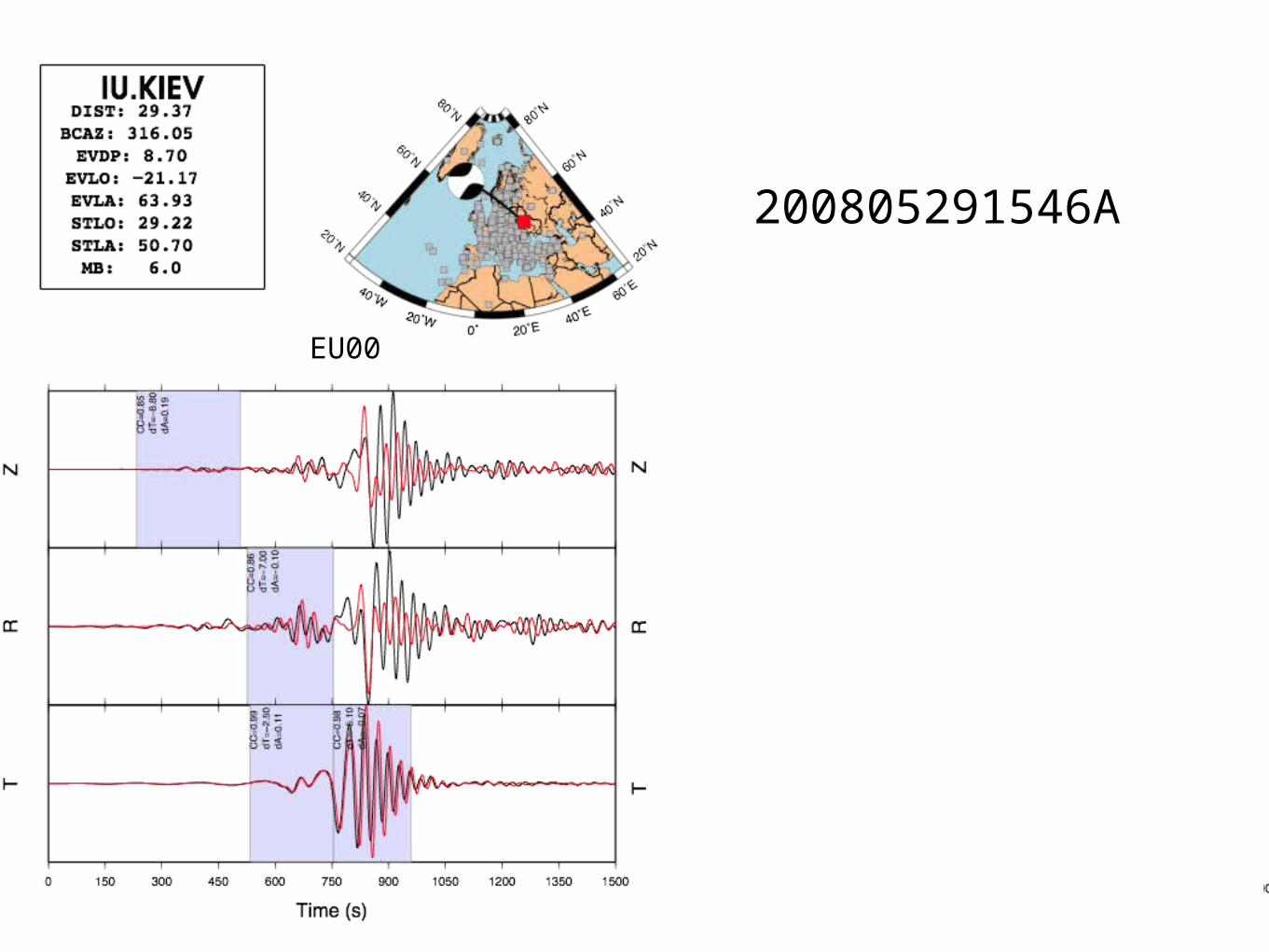
200805291546A

EU00 EU30

Goal:

Fitting frequency-dependent phase and amplitude anomalies in targeted windows

automated window selection: FLEXWIN (Maggi et al. 2009)

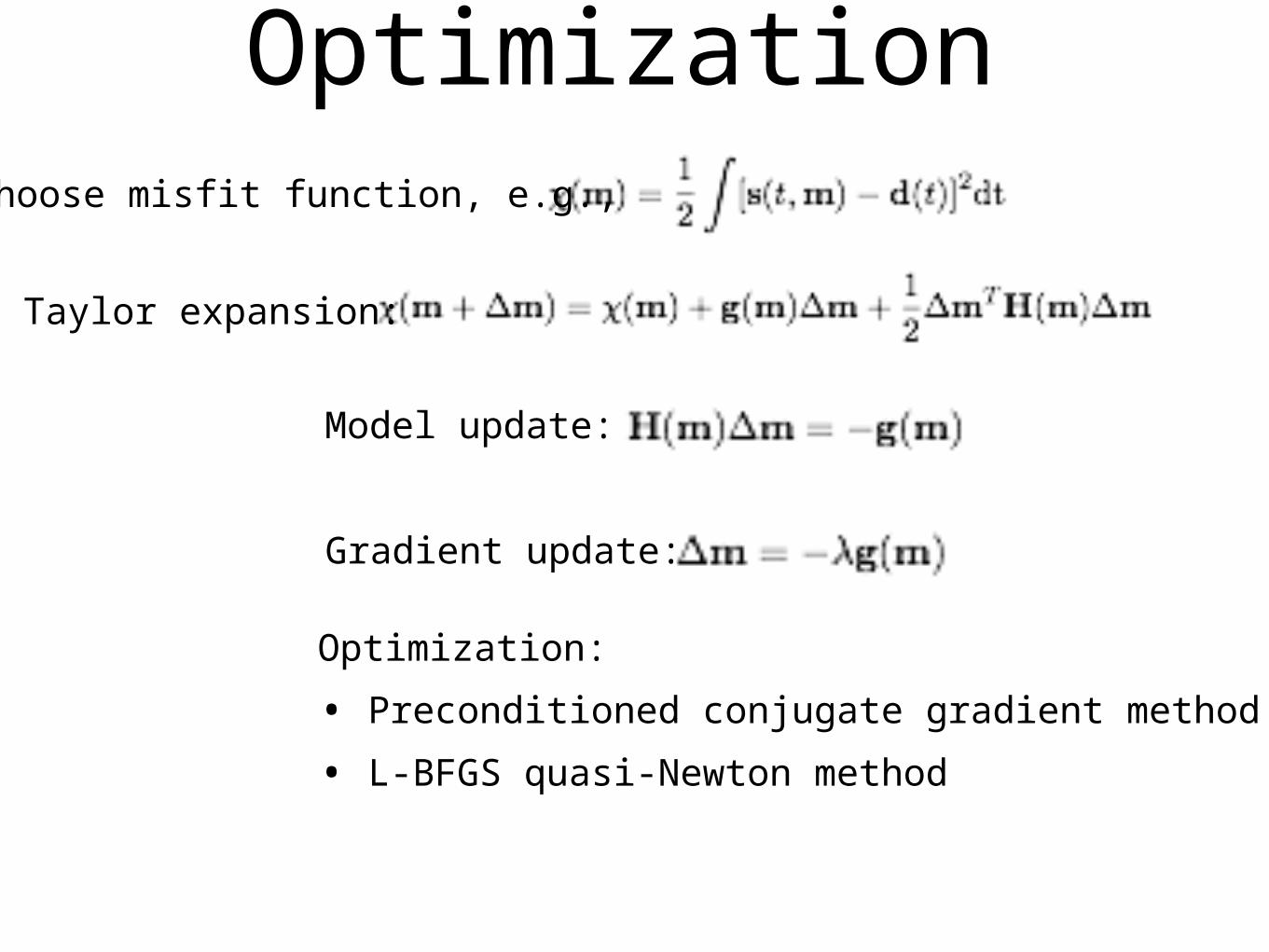
Optimization

Taylor expansion:

Choose misfit function, e.g.,

Model update:

Gradient update:

Optimization:

• Preconditioned conjugate gradient method

• L-BFGS quasi-Newton method

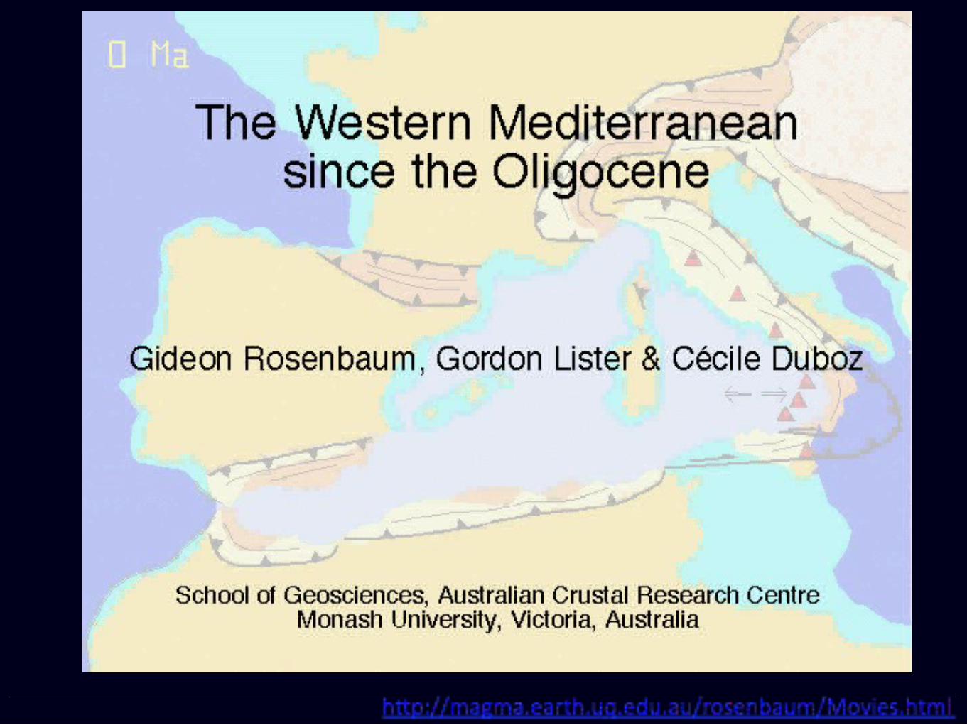
Wortel & Spakman (2000)

Mediterranean-Calabria Paleotectonics

Depth 75 km

Middle Hungarian line

Pannonian Basin

Massif Central

Central graben

Armorican Massif

Harz

Tornquist-Teisseyre Zone

Bohemian massif

Central Slovakian volcanic field

Eifel hotspot & Rhine graben

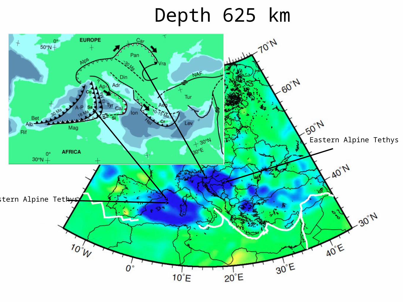
Depth 625 km

Eastern Alpine Tethys

Western Alpine Tethys

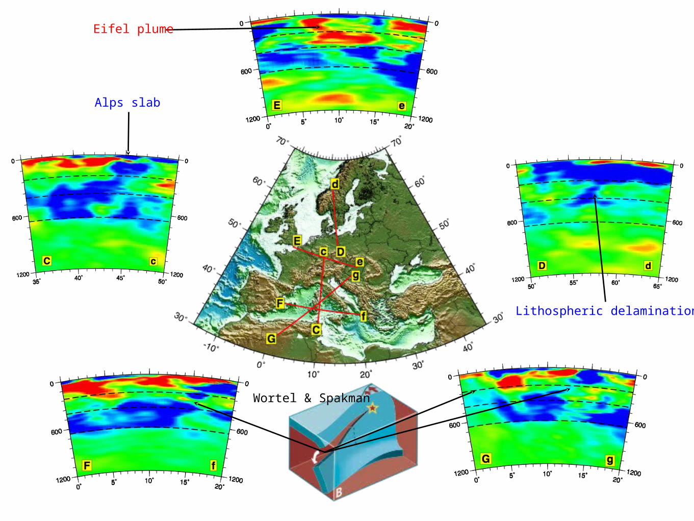
Wortel & Spakman

Alps slab

Eifel plume

Lithospheric delamination

200805291546A

EU00 EU30

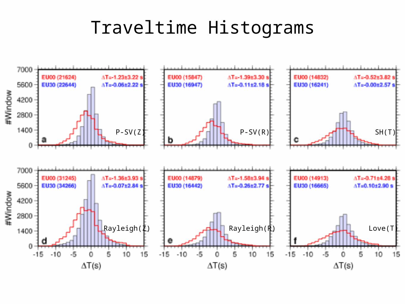
Traveltime Histograms

P-SV(Z) P-SV(R) SH(T)

Rayleigh(Z) Rayleigh(R) Love(T)

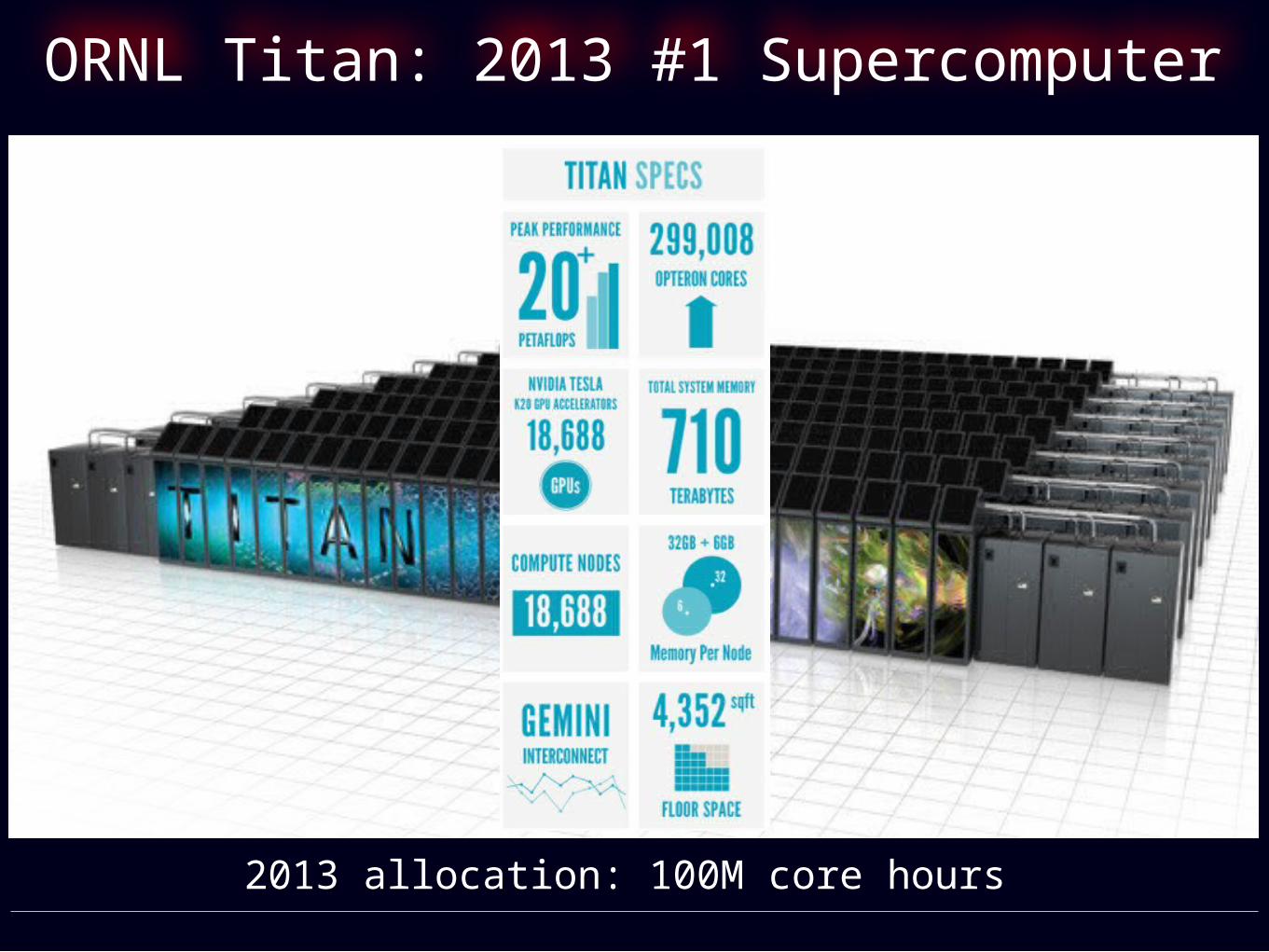
ORNL Titan: 2013 #1 Supercomputer

2013 allocation: 100M core hours

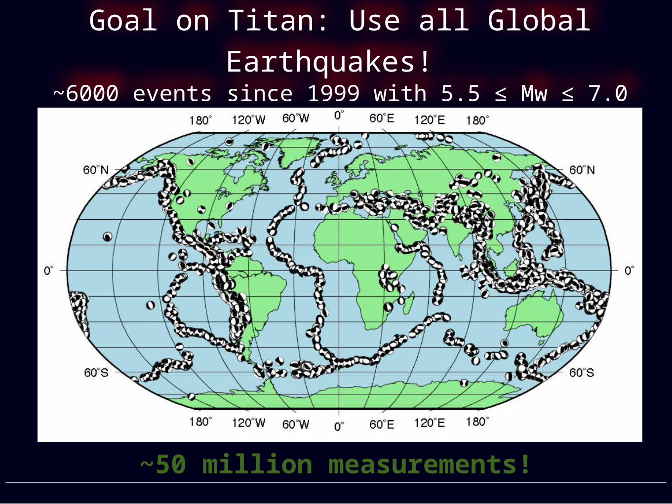
Goal on Titan: Use all Global Earthquakes! ~6000 events since 1999 with 5.5 ≤ Mw ≤ 7.0

~50 million measurements!

Conclusions• Modern numerical methods and computers are used to simulate

seismic wave propagation in 3D Earth models

• Adjoint methods are used to calculate misfit gradients in 3D Earth

models

• We are bridging the gap between high-resolution body-wave

tomography and lower resolution inversions based on long-period

body waves, surface waves and free oscillations

• Simultaneous analysis of wavespeeds, attenuation and anisotropy

will improve our understanding of temperature, composition, partial

melting and water contents within the Earth’s interior