1 INTRODUCTION The analysis of seismic site response is very important since seismic waves can be significantly modified

when travelling through soils. Local site effects profoundly influence many crucial characteristics of strong ground motions. During the 1985 Mexico, 1989 Loma Prieta and 1995 Kobe earthquakes, significant damage and loss of life were directly attributed to the amplification of ground motion due to local site conditions (Frankel 1991, Kawase 1997, Flores-Estrella 2007). A lot of field tests and numerical simulations have been used to study this phenomenon. Conventional numerical methods are often performed using equivalent linear procedures with the assumption of one-dimensional soil model, such as the site response software SHAKE (Schnabel 1972). However, the soil can be a highly heterogeneous medium. 2D or 3D models are more ap-propriate to account for the spatial difference of local sites. Thompson et al. (2009) demonstrated that for some cases, one-dimensional assumption does not hold. However, in their research, they did not consider the correlation-distance difference between horizontal and vertical directions. The computation is also very ex-pensive due to the use of finite difference method in their study. In this study, displacement boundary is used for input of vertically incident plane wave and soil shear modulus is modelled as spatially random field with correlation distances in horizontal and vertical directions. Amplification factors are then used to explore the influence of heterogeneity on local site response.

2 METHODS In this study, Spectral Element Method (SEM) is used for the simulation of seismic wave propagation in a

heterogeneous medium. The main advantage of SEM is that it combines the flexibility of finite element meth-od and the accuracy of pseudospectral techniques (Komatitsch et al. 2004). Here in this paper we use the software package SPECFEM2D developed by Komatitsch & Vilotte (1998). To address the problem which is of our concern, we implemented displacement boundary in this software package.

The Twenty-Eight KKHTCNN Symposium on Civil Engineering

November 16-18, 2015, Bangkok, Thailand

Seismic Response Analysis of Heterogeneous Soils Using 2D Spectral Element Method

Chunyang DU1 and Gang WANG1

1Department of Civil and Environmental Engineering, Hong Kong University of Science and Technology, Hong Kong SAR

cdu@ust.hk, gwang@ust.hk

ABSTRACT

Seismic waves can be significantly modified during wave propagation through soils. Conventional ground response analysis usually assumes the soils are horizontally layered, without considering heterogeneous dis-tribution of soil properties. In this study, wave propagation through heterogeneous soils is numerically simu-lated using the 2D Spectral Element Method. The shear wave velocity of the soils is modelled as a spatially correlated random field. Under an incident plane Ricker wavelet, amplification factors of surface motions at different locations are studied by varying the variation of shear wave velocities of the soils and their correla-tion distances in horizontal and vertical directions. Compared with a uniform soil profile, increase in soil het-erogeneity lowers the resonance frequencies of the site, also results in reduced amplification factors at high frequencies. The correlation distances of the shear wave velocities also affect the variation of amplification factors of the heterogeneous site.

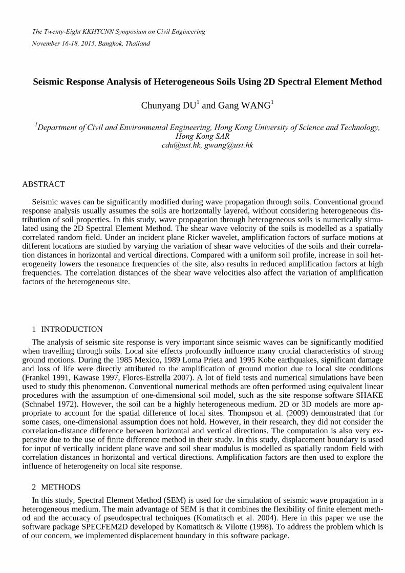
A series of standard linear solids (Figure 1.) is used in the software to mimic a viscoelastic medium. In practice, 2 to 3 standard linear solids can generate an almost constant attenuation medium (Savage 2010). In our simulations, 4 standard linear solids are used to achieve 5% damping ratio in the frequency range from 0.1Hz to 30Hz which is the main frequency content of earthquake waves (Figure 2.(a)). Meanwhile, for this model, the shear modulus is frequency dependent. Slight increase from the set value of 200m/s can be seen in the shear wave velocity for high frequency due to the choice of this mechanical model (Figure 2.(b)).

11k 12k 1Lk

21k 22k 2 Lk1η 2η Lη

σ

σ

ε

10

−410

−210

010

210

40

0.02

0.04

0.06

0.08

0.1

0.12

Frequency, HzD

issi

patio

n Fa

ctor

10

−410

−210

010

210

4

180

190

200

210

220

Frequency, Hz

Phas

e V

eloc

ity, m

/s

a. Dissipation factor. b. Phase velocity. Figure 1. Standard linear solids. Figure 2. Mechanical properties of standard linear solids.

To investigate the influence of soil heterogeneity, we modelled soil shear velocity as spatially correlated

random field. The shear velocity follows lognormal distribution. Four parameters are used to quantify the spa-tially correlated random field which are mean shear wave velocity Vs, standard deviation of lnVs, horizontal correlation distance hr and vertical correlation distance hv. Figure 3. gives a typical illustration of spatially correlation random field with different horizontal and vertical correlation distances.

−50 0 50

−30

−20

−10

0V

s m/s

X,m

Y,m

150200250

−50 0 50

−30

−20

−10

0V

s m/s

X,m

Y,m

150200250

−50 0 50

−30

−20

−10

0V

s m/s

X,m

Y

,m150200250

a. hr =2m, hv =2m b. hr =50m, hv =2m c. hr =50m, hv =10m

Figure 3. Spatially correlated random field. Mean value Vs =200m/s, standard deviation of lnVs =0.2.

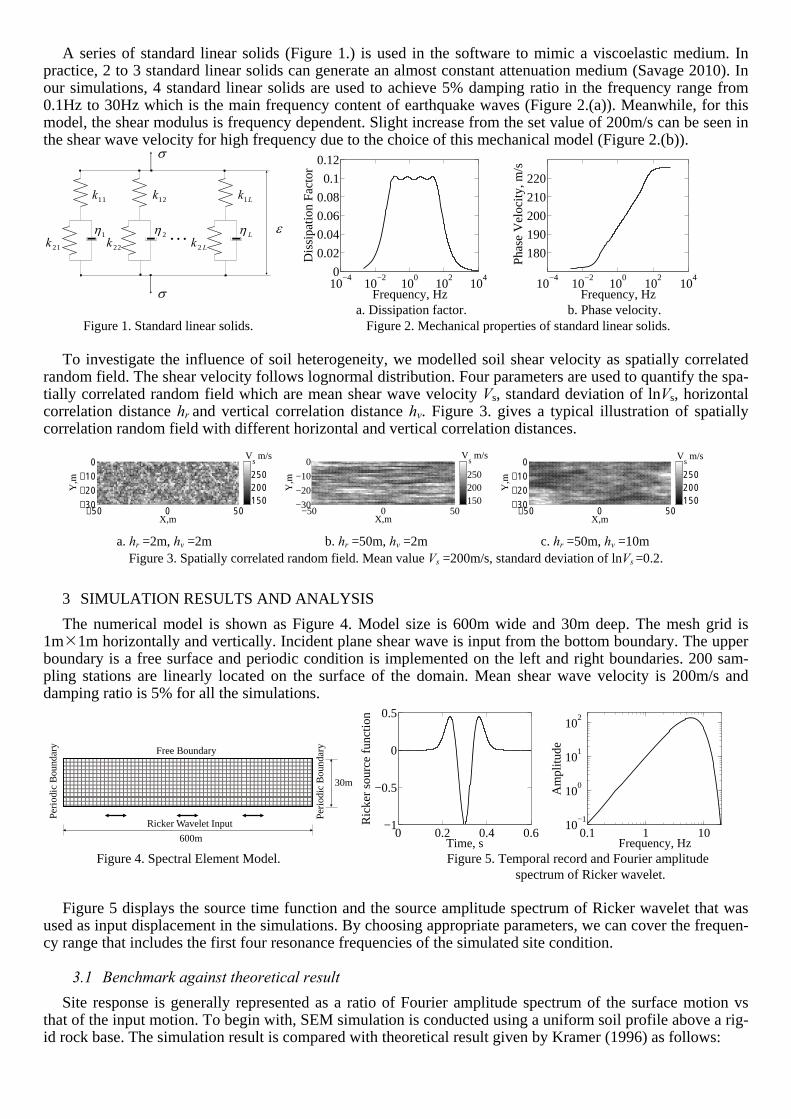
3 SIMULATION RESULTS AND ANALYSIS The numerical model is shown as Figure 4. Model size is 600m wide and 30m deep. The mesh grid is

1m 1m horizontally and vertically. Incident plane shear wave is input from the bottom boundary. The upper boundary is a free surface and periodic condition is implemented on the left and right boundaries. 200 sam-pling stations are linearly located on the surface of the domain. Mean shear wave velocity is 200m/s and damping ratio is 5% for all the simulations.

Free Boundary

Perio

dic

Bou

ndar

y

30m

600m

Perio

dic

Bou

ndar

y

Ricker Wavelet Input0 0.2 0.4 0.6

−1

−0.5

0

0.5

Time, s

Ric

ker

sour

ce f

unct

ion

0.1 1 1010

−1

100

101

102

Frequency, Hz

Am

plitu

de

Figure 4. Spectral Element Model. Figure 5. Temporal record and Fourier amplitude spectrum of Ricker wavelet.

Figure 5 displays the source time function and the source amplitude spectrum of Ricker wavelet that was

used as input displacement in the simulations. By choosing appropriate parameters, we can cover the frequen-cy range that includes the first four resonance frequencies of the simulated site condition.

3.1 Benchmark against theoretical result

Site response is generally represented as a ratio of Fourier amplitude spectrum of the surface motion vs that of the input motion. To begin with, SEM simulation is conducted using a uniform soil profile above a rig-id rock base. The simulation result is compared with theoretical result given by Kramer (1996) as follows:

( ) ( )( )

( )

1, 0,

cos1

u t zf

u t z H HV is

αω

ξ

==

=+

= (1)

where ω = wave angular frequency; H = soil depth; and Vs = soil shear velocity (200m/s); ξ is damping ratio (5%). This theoretical function is used to benchmark our simulations.

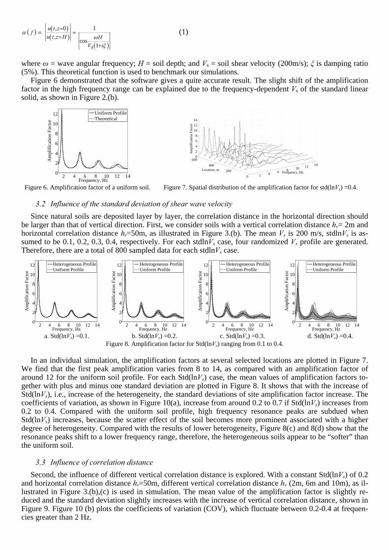
Figure 6 demonstrated that the software gives a quite accurate result. The slight shift of the amplification factor in the high frequency range can be explained due to the frequency-dependent Vs of the standard linear solid, as shown in Figure 2.(b).

2 4 6 8 10 12 14

0

2

4

6

8

10

12

Frequency, Hz

Am

plif

icat

ion

Fact

or

Uniform ProfileTheoretical

2 4 6 8 10 12 14

0

200

400

6000

2

4

6

8

10

12

14

Frequency, HzLocation, m

Am

plif

icat

ion

Fact

or

Figure 6. Amplification factor of a uniform soil. Figure 7. Spatial distribution of the amplification factor for std(lnVs) =0.4.

3.2 Influence of the standard deviation of shear wave velocity

Since natural soils are deposited layer by layer, the correlation distance in the horizontal direction should be larger than that of vertical direction. First, we consider soils with a vertical correlation distance hv= 2m and horizontal correlation distance hr=50m, as illustrated in Figure 3.(b). The mean Vs is 200 m/s, stdlnVs is as-sumed to be 0.1, 0.2, 0.3, 0.4, respectively. For each stdlnVs case, four randomized Vs profile are generated. Therefore, there are a total of 800 sampled data for each stdlnVs case.

2 4 6 8 10 12 140

2

4

6

8

10

12

Frequency, Hz

Am

plif

icat

ion

Fact

or

Heterogeneous ProfileUniform Profile

2 4 6 8 10 12 140

2

4

6

8

10

12

Frequency, Hz

Am

plif

icat

ion

Fact

or

Heterogeneous ProfileUniform Profile

2 4 6 8 10 12 140

2

4

6

8

10

12

Frequency, Hz

Am

plif

icat

ion

Fact

or

Heterogeneous ProfileUniform Profile

2 4 6 8 10 12 140

2

4

6

8

10

12

Frequency, Hz

Am

plif

icat

ion

Fact

or

Heterogeneous ProfileUniform Profile

a. Std(lnVs) =0.1. b. Std(lnVs) =0.2. c. Std(lnVs) =0.3. d. Std(lnVs) =0.4.

Figure 8. Amplification factor for Std(lnVs) ranging from 0.1 to 0.4. In an individual simulation, the amplification factors at several selected locations are plotted in Figure 7.

We find that the first peak amplification varies from 8 to 14, as compared with an amplification factor of around 12 for the uniform soil profile. For each Std(lnVs) case, the mean values of amplification factors to-gether with plus and minus one standard deviation are plotted in Figure 8. It shows that with the increase of Std(lnVs), i.e., increase of the heterogeneity, the standard deviations of site amplification factor increase. The coefficients of variation, as shown in Figure 10(a), increase from around 0.2 to 0.7 if Std(lnVs) increases from 0.2 to 0.4. Compared with the uniform soil profile, high frequency resonance peaks are subdued when Std(lnVs) increases, because the scatter effect of the soil becomes more prominent associated with a higher degree of heterogeneity. Compared with the results of lower heterogeneity, Figure 8(c) and 8(d) show that the resonance peaks shift to a lower frequency range, therefore, the heterogeneous soils appear to be “softer” than the uniform soil.

3.3 Influence of correlation distance

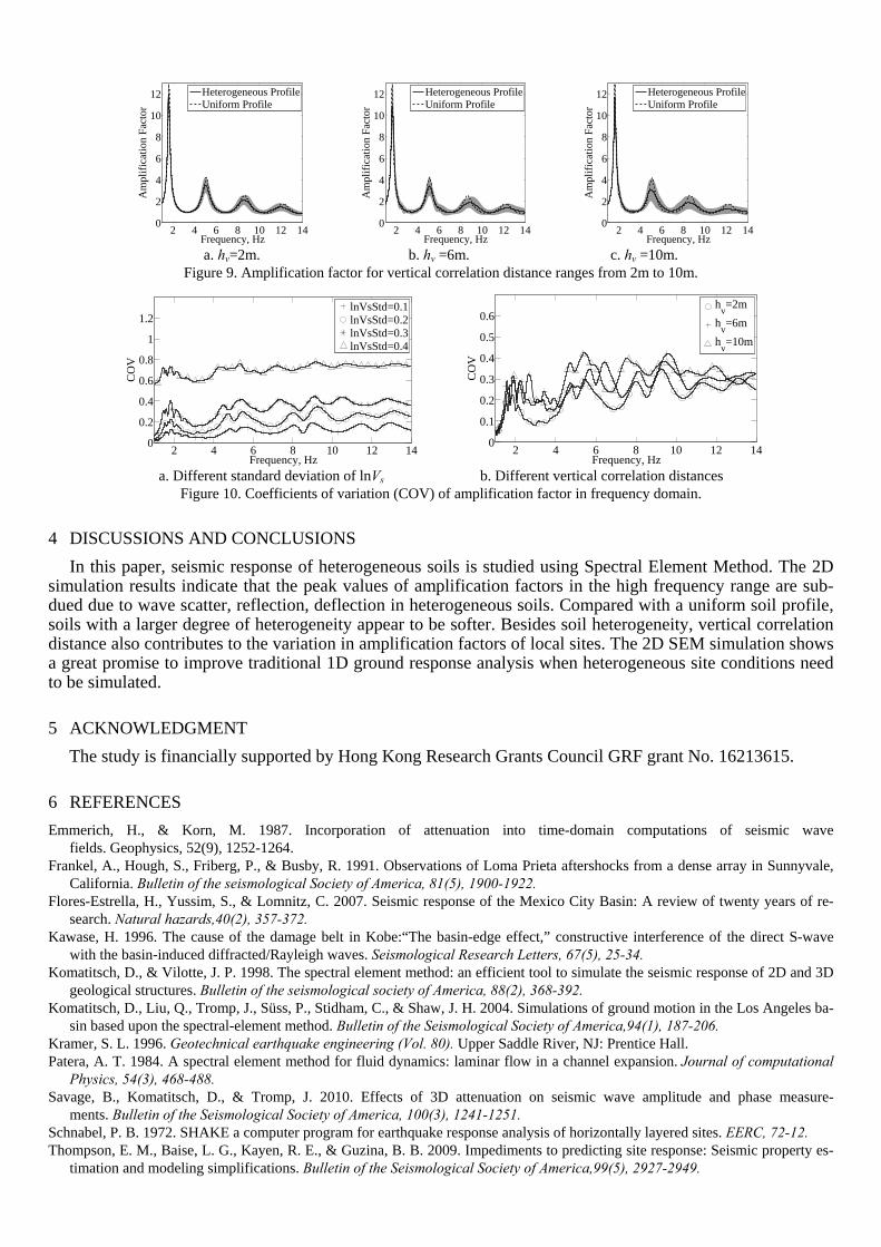
Second, the influence of different vertical correlation distance is explored. With a constant Std(lnVs) of 0.2 and horizontal correlation distance hr=50m, different vertical correlation distance hv (2m, 6m and 10m), as il-lustrated in Figure 3.(b),(c) is used in simulation. The mean value of the amplification factor is slightly re-duced and the standard deviation slightly increases with the increase of vertical correlation distance, shown in Figure 9. Figure 10 (b) plots the coefficients of variation (COV), which fluctuate between 0.2-0.4 at frequen-cies greater than 2 Hz.

2 4 6 8 10 12 140

2

4

6

8

10

12

Frequency, Hz

Am

plif

icat

ion

Fact

or

Heterogeneous ProfileUniform Profile

2 4 6 8 10 12 140

2

4

6

8

10

12

Frequency, Hz

Am

plif

icat

ion

Fact

or

Heterogeneous ProfileUniform Profile

2 4 6 8 10 12 140

2

4

6

8

10

12

Frequency, Hz

Am

plif

icat

ion

Fact

or

Heterogeneous ProfileUniform Profile

a. hv=2m. b. hv =6m. c. hv =10m.

Figure 9. Amplification factor for vertical correlation distance ranges from 2m to 10m.

2 4 6 8 10 12 14

0

0.2

0.4

0.6

0.8

1

1.2

Frequency, Hz

CO

V

lnVsStd=0.1lnVsStd=0.2lnVsStd=0.3lnVsStd=0.4

2 4 6 8 10 12 14

0

0.1

0.2

0.3

0.4

0.5

0.6

Frequency, HzC

OV

hv=2m

hv=6m

hv=10m

a. Different standard deviation of lnVs b. Different vertical correlation distances

Figure 10. Coefficients of variation (COV) of amplification factor in frequency domain.

4 DISCUSSIONS AND CONCLUSIONS In this paper, seismic response of heterogeneous soils is studied using Spectral Element Method. The 2D

simulation results indicate that the peak values of amplification factors in the high frequency range are sub-dued due to wave scatter, reflection, deflection in heterogeneous soils. Compared with a uniform soil profile, soils with a larger degree of heterogeneity appear to be softer. Besides soil heterogeneity, vertical correlation distance also contributes to the variation in amplification factors of local sites. The 2D SEM simulation shows a great promise to improve traditional 1D ground response analysis when heterogeneous site conditions need to be simulated.

5 ACKNOWLEDGMENT The study is financially supported by Hong Kong Research Grants Council GRF grant No. 16213615.

6 REFERENCES Emmerich, H., & Korn, M. 1987. Incorporation of attenuation into time-domain computations of seismic wave

fields. Geophysics, 52(9), 1252-1264. Frankel, A., Hough, S., Friberg, P., & Busby, R. 1991. Observations of Loma Prieta aftershocks from a dense array in Sunnyvale,

California. Bulletin of the seismological Society of America, 81(5), 1900-1922. Flores-Estrella, H., Yussim, S., & Lomnitz, C. 2007. Seismic response of the Mexico City Basin: A review of twenty years of re-

search. Natural hazards,40(2), 357-372. Kawase, H. 1996. The cause of the damage belt in Kobe:“The basin-edge effect,” constructive interference of the direct S-wave

with the basin-induced diffracted/Rayleigh waves. Seismological Research Letters, 67(5), 25-34. Komatitsch, D., & Vilotte, J. P. 1998. The spectral element method: an efficient tool to simulate the seismic response of 2D and 3D

geological structures. Bulletin of the seismological society of America, 88(2), 368-392. Komatitsch, D., Liu, Q., Tromp, J., Süss, P., Stidham, C., & Shaw, J. H. 2004. Simulations of ground motion in the Los Angeles ba-

sin based upon the spectral-element method. Bulletin of the Seismological Society of America,94(1), 187-206. Kramer, S. L. 1996. Geotechnical earthquake engineering (Vol. 80). Upper Saddle River, NJ: Prentice Hall. Patera, A. T. 1984. A spectral element method for fluid dynamics: laminar flow in a channel expansion. Journal of computational

Physics, 54(3), 468-488. Savage, B., Komatitsch, D., & Tromp, J. 2010. Effects of 3D attenuation on seismic wave amplitude and phase measure-

ments. Bulletin of the Seismological Society of America, 100(3), 1241-1251. Schnabel, P. B. 1972. SHAKE a computer program for earthquake response analysis of horizontally layered sites. EERC, 72-12. Thompson, E. M., Baise, L. G., Kayen, R. E., & Guzina, B. B. 2009. Impediments to predicting site response: Seismic property es-

timation and modeling simplifications. Bulletin of the Seismological Society of America,99(5), 2927-2949.