Seismic inversion methods and some of their … · Introduction The interest in seismic inversion...

© 2004 EAGE 47

technical article

IntroductionThe interest in seismic inversion techniques has been growingsteadily over the last couple of years. Integrated studies areessential to hydrocarbon development projects (e.g. Vazquez etal. 1997, Cosentino 2001) and inversion is one of the meansto extract additional information from seismic data. Variousseismic inversion techniques are briefly presented. Inversionreplaces the seismic signature by a blocky response, correspon-ding to acoustic and/or elastic impedance layering. It facilitatesthe interpretation of meaningful geological and petrophysicalboundaries in the subsurface. Inversion increases the resolu-tion of conventional seismics in many cases and puts the studyof reservoir parameters at a different level. It results in opti-mised volumetrics, improved ranking of leads/prospects, betterdelineation of drainage areas and identification of ‘sweetspots’ in field development studies (e.g. Veeken et al. 2002).

The main steps in an inversion study are: ■ Quality control and pre-conditioning of the input data.■ Well–to-seismic match, zero-phasing of data in zone of

interest and extraction of the wavelet.■ Running of the inversion algorithm with generation of

acoustic or elastic impedance cubes and extraction ofattributes.

■ Visualisation and interpretation of the results in terms ofreservoir development.

The inversion methods are either deterministic or probabilisticand the approach can be post- and/or pre-stack. Inversionschemes generally use migrated time data as basic input. Thepre-stack method exploits AVO effects on migrated CDP gath-ers. There is a trade-off between method/cost/time and qualityof inversion results. Feasibility studies with synthetic model-ling are recommended before embarking on an inversion orAVO project (Da Silva et al., in prep.).

The past track record has demonstrated the benefits of theseismic inversion method. However, it should be realised thatthe inversion procedure is not a unique process, i.e. there is nosingle solution to the given problem. Care should be takenwhen interpreting the inversion results. Adequate data pre-conditioning is a prerequisite for quantitative interpretation ofthe end results.

Deconvolution and seismic inversion.Seismic inversion is undertaken to complement conventionaldeconvolution processing. Deconvolution tries to undo some

negative effects of the seismic convolution. It is in general suc-cessful in reducing multiple energy (Yilmaz 2001). Duringacquisition of reflection datasets, the seismic signal is sentthrough the earth (i.e. convolved with the earth filter) andreflected back into the geophone (convolved with the record-ing set-up filter). Deconvolution is meant to undo the defor-mation caused by these two filters to the seismic response. Aspiked response is never achieved because of the band limitednature of the seismic data (Veeken, in prep.). The decon filterwould need to be infinitely long, which is clearly not feasible.A perfect job is therefore hardly ever possible and that is whereseismic inversion or stratigraphic deconvolution comes in.

Ideally, an acoustic impedance interface should be repre-sented by a single spike on the seismic trace. The contrast isdescribed by the reflectivity formula:

(1)

Acoustic impedance interfaces in the real world are sometimespositioned very closely together. As a result, the seismicresponse of the first interface overlaps in time with the energytriggered by the next interface. The result is interference of theindividual seismic events on the recorded seismogram. A com-posite seismic loop is registered in the geophone at the surface(Figure 1A). Under these circumstances it becomes difficult todiscriminate between the effects stemming from each interface.Therefore, the apparent amplitude and frequency of reflectionsshould always be treated with care during the interpretationphase (Veeken, in prep.).

It is necessary to undertake ‘stratigraphic deconvolution’to undo some of the negative interference effects (cf Duboz etal. 1998). This technique is also known as seismic inversion.The seismic signature is replaced by a blocky response corre-sponding to the seismic impedance layering. This type of pro-cessing facilitates the interpretation of meaningful geologicaland petrophysical boundaries on the reflection data (Veeken etal. 2002). The input for seismic inversion is traditionally com-posed of time migrated seismic data (pre- or post-stack), awavelet and an optional initial earth model (velocities anddensities; Figure 1B). Inversion allows the study of reservoircharacteristics in greater detail, under favourable circum-stances the resolution of the dataset is even increased.Detection of thin beds is based on subtle changes in the shapeof a specific seismic loop (doublet), a feature that is usuallybeyond the standard seismic resolution.

It is recommendable that prestack time migration data

R = ( 2V2 - 1V1) / ( 2V2 + 1V1)

first break volume 22, June 2004

Seismic inversion methods and some of theirconstraintsP. C. H. Veeken and M. Da Silva*

* P.C.H. Veeken, 29 rue des Benedictins, 57050 Le Ban St. Martin, FranceM. da Silva, 1 rue Léon Migaux, 91341 Massy CEDEX, France

© 2004 EAGE48

technical article first break volume 22, June 2004

Composite seismic loops

A )

Impedance Cube

OUTPUT INVERSION

3D seismic data

Seismic

waveletInitial impedance

model

INPUT

Picked Horizons

in TWT

B )

Figure 1B The input for a model-driven seismic inversion consists of time migrated seismic data, a seismic wavelet, an option-al impedance model and picked time horizons. Proper data conditioning is a pre-requisite to obtain reliable results. Seismicinversion is never a unique process, i.e. there is not a single solution to the given problem, but several models may equallywell explain the recorded seismic response.

Figure 1A Thin bed configuration givesrise to a composite seismic response dueto time overlap and interference of thereflected seismic pulses (modified afterTodd and Sangree, 1977).

© 2004 EAGE 49

technical article

serves as input to the inversion scheme. The main advantage isa substantially better velocity field and improved positioningof the reflections. The corresponding interval velocity model isin general more detailed than that obtained via the conven-tional seismic method exploiting Dix's formula (Dix 1955).Moreover, this velocity field is better suited for evaluation ofin-situ geo-pressures and fault compartment predictions (e.g.

Dutta 2002; Figure 2). Inversion is often done in conjunction with AVO analysis.

The combination of these geophysical study techniques aug-ments the confidence in correct ranking of leads / prospectsand definition of ‘sweet spots’ in the HC accumulations(Veeken et al. 2002). Such an approach reduces uncertaintiesand drilling risks, which is an important aspect for optimising


Figure 2 The pre-stack seismic inversion results in a better velocity model. The interval velocities calculated via Dix's formu-la are very smooth and therefore less reliable. It ensures the best stack, but does not yield necessarily the best interval veloc-ity. The inversion involves a pre-stack time migration and this velocity model preserves better the original variability of thevelocity field (modified after Dutta 2002).

© 2004 EAGE50

technical article

an exploration and hydrocarbon development strategy (DaSilva et al., in prep). A pre-stack inversion scheme incorporatesAVO effects seen on CDP gathers. The partial stacks (PS) showin many cases a characteristic difference in behaviour for theamplitude of the top hydrocarbon reservoir reflection (AVOeffect). The P- and S-wave energy are crucial parameters tomodel the reflectivity of synthetic offset gathers.Compressional P-waves contain information on the lithologyand the porefill, while transverse S-waves are hardly influ-enced by the fluid contents. Absence of P-wave related DHIson the corresponding S-sections is, for instance, a useful crite-rion to discriminate between a hydrocarbon and brine filledreservoir (Stewart et al. 2003). Rock physical parameters likethe Poisson's ratio, rhomu, lambdarho are estimated from theP- and S-wave velocity variations. The prestack inversion givesa better handle on the lithology, porosity, permeability and/orwater saturation in the porefill of the rocks under investiga-tion.

Stratigraphic deconvolution tries to put a simple spikedreflectivity response at geological boundaries (lithologicalchanges) and the main reservoir interfaces (for instance, a fluidcontact). This is often done by inversion of the seismic cubeinto an acoustic impedance cube (Figure 1B). The acoustic

impedance of a rock sequence is defined as the product of den-sity and velocity (cf Sheriff 2002). The link between the seis-mic and acoustic impedance (AI) cube is the seismic wavelet.The wavelet is derived either directly from the seismic data orcomputed with the aid of available well data. The density andsonic logs in the well permit calculation of the AI response.Calibrated sonic with checkshots and/or VSP data are neededfor the depth-time conversion of the vertical log scale. The realseismic trace at the well location is subsequently matched withthe reflectivity trace computed from the well logs. This com-parison yields the seismic wavelet.

A typical inversion project generally comprises the followingsteps:■ Quality control and pre-conditioning of the input data.■ Well–to-seismic match and compilation of a synthetic trace.■ Zero-phasing of data in zone of interest and extraction of

the wavelet. This step can be circumvented when the nonzero-phase effects are integrated in the wavelet used for theinversion.

■ Running of the inversion algorithm.■ Visualisation and interpretation of the results in terms of

reservoir development.


Migrated NMO-corrected CDP gather

with mute function

4 bad traces 6 bad traces

Raw stack Muted stack

Blanked data above yellow line

Preserved data below yellow lineA ) B )

Zero offset comparison

Figure 3A Mute function applied on a CDP gather. Data from a specific offset and time range is used for each time samplein the processing. In this way the amount of noise on the traces is drastically reduced. Selection of the proper mute functionis critical in optimising the stacking results.Figure 3B Comparison of a raw stacked seismic line and the same line whereby the mute function is applied on the CDPgathers before the stack.

© 2004 EAGE 51

technical article

Seismic inversion is a somewhat confusing expression.Inversion in itself means to undo an operation, but here itrepresents the transformation of a seismic amplitude cubeinto an acoustic (or elastic) impedance cube. There are sever-al ways to achieve this objective, as will be shown later on.

Time lapse inversion of 4D seismics and reservoir behav-iour monitoring facilitate the extraction of saturation andpressure effects induced by hydrocarbon production (e.g.Gluck 2000, Oldenziel 2003).

Input data conditioningIt is important that the seismic input data are screened fortheir quality. In a pre-stack approach it means going back tothe CDP gathers and making sure that the panels are clean.It might prove necessary to apply a more efficient mute func-tion for this purpose (Figure 3). Simple bandpass filtering canbe very effective for improving the seismic data. Applying aspiking random noise attenuator is a more sophisticated wayto reduce the noise on the migrated stack. A 3D filteringapproach will give even better results (Da Silva et al., inprep).

The acquisition footprint is often difficult to remove in3D surveys, but it is an essential step for reconstituting thetrue amplitude character of a dataset. The aim is to preservethe real amplitude behaviour proportional to the acousticimpedance contrasts in the subsurface and eliminate anyknown amplitude distortions. These amplitude correctionsshould be implemented when it enhances the overall qualityof the seismic dataset. Whitening of the amplitude spectra isin this respect sometimes a dangerous operation that needscareful evaluation before it is done. Whitening means thatthe amplitudes for all frequencies are adjusted to the sameoutput level. This artificial amplitude boosting is in manycases rather uncontrolled and accompanied by a significantand unacceptable increase in noise level.

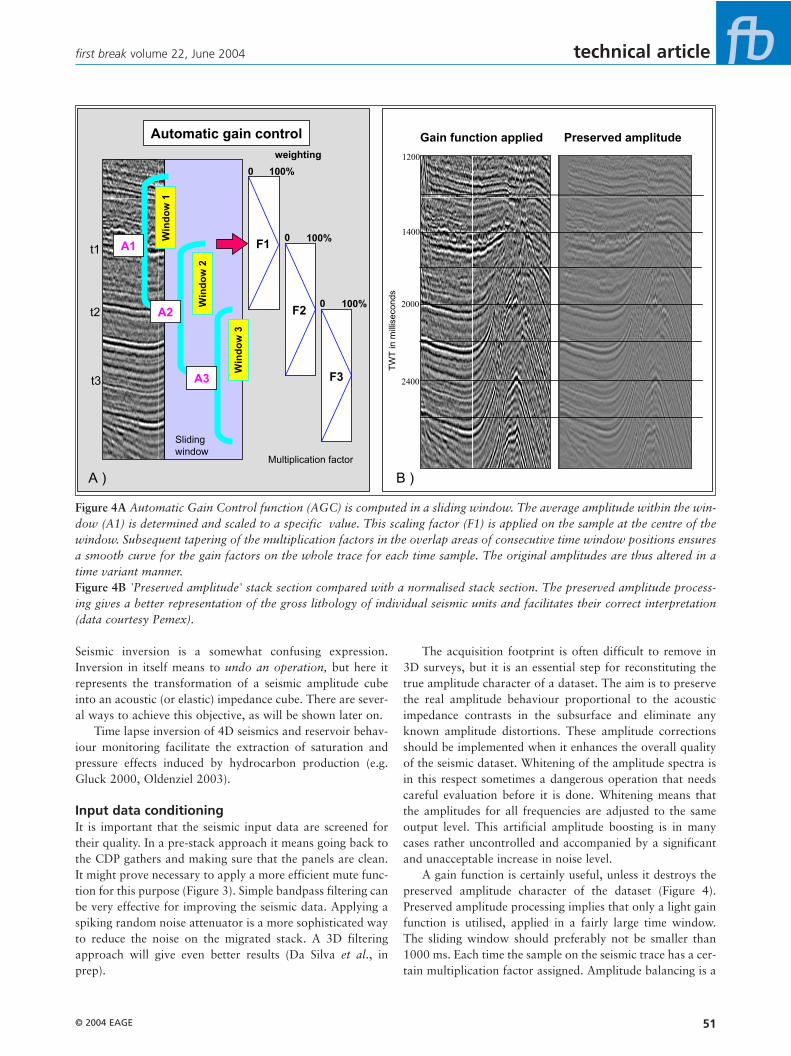
A gain function is certainly useful, unless it destroys thepreserved amplitude character of the dataset (Figure 4).Preserved amplitude processing implies that only a light gainfunction is utilised, applied in a fairly large time window.The sliding window should preferably not be smaller than1000 ms. Each time the sample on the seismic trace has a cer-tain multiplication factor assigned. Amplitude balancing is a


A1

A2

A3

0 100%

0 100%

0 100%

Win

do

w1

Win

do

w2

Win

do

w3

F1

F2

F3

Automatic gain control

t1

t2

t3

Multiplication factor

weighting

Sliding

window

2000

1400

2400

Preserved amplitudeGain function applied

TW

T in m

illis

econds

1200

A ) B )

Figure 4A Automatic Gain Control function (AGC) is computed in a sliding window. The average amplitude within the win-dow (A1) is determined and scaled to a specific value. This scaling factor (F1) is applied on the sample at the centre of thewindow. Subsequent tapering of the multiplication factors in the overlap areas of consecutive time window positions ensuresa smooth curve for the gain factors on the whole trace for each time sample. The original amplitudes are thus altered in atime variant manner.Figure 4B 'Preserved amplitude' stack section compared with a normalised stack section. The preserved amplitude process-ing gives a better representation of the gross lithology of individual seismic units and facilitates their correct interpretation(data courtesy Pemex).

© 2004 EAGE52

technical article

delicate process that should be done with care, especiallywhen later quantitative interpretation is the ultimate goal(Veeken, in prep.).

Even velocity filtering is worthwhile considering on thecondition that the F-K operation cuts out only noise (Figure5). Under such circumstances the F-K filter will indeed alterthe amplitudes, but in a good sense. The latter has to bedemonstrated by proper testing of the processing parameters.Multiple suppression and deconvolution are other issues thatneed to be addressed in order to clean up the data. Radontransform or Tau-P processing is an alternative option, a lastresort when other methods fail to enhance the dataset. TheTau stands for intercept time at the zero offset position. P isthe slowness parameter of the ray in Snell's Law. Seismicnoise is sometimes more easily removed in the Tau-P domain.A drawback is that the transform back to the TX domain israther sensitive to errors, because the operator is not orthog-onal (Trad et al. 2003). Furthermore, the Radon Transformsuffers from loss of resolution and aliasing, arising fromincompleteness of information due to limited aperture anddiscretization of the data or time sampling (Querne, pers.com.).

In general, multiples are bad news because inversion willtreat them as primaries. Aggressive de-multiple operators,however, may cause unwanted damage to the primaries.Decisions on the correct trade-off are usually made on reflec-

tivity sections. The suppression test results may look differ-ent in the pre-stack domain. Hence, combined pre- and post-stack testing is recommendable for multiple suppression.Artefacts in the input data clearly will lead to unreliableinversion results. Multiple suppression, amplitude balancingand true amplitude processing are closely related subjectsthat highly influence the inversion end-results. A preservedamplitude section often looks different from a section thatpleases the interpreter’s eye. The ideal input to seismic inver-sion are of course amplitudes that are directly proportionalto the subsurface reflection coefficients.

Proper data conditioning is essential for later quantitativeinterpretation of the inversion end results, i.e. when reservoircharacterisation and lateral prediction studies are required(Da Silva et al., in prep). For that matter reprocessing of theseismic dataset may prove necessary; even complete re-shoots are sometimes justified (e.g. Onderwater et al. 1996).The original data was processed with a special target in mindand all parameters were tuned to this objective. The later useof the same seismic dataset in pre-stack analysis was unfor-tunately not always foreseen. Pre-stack time migrationresults in better positioned seismic energy and also the veloc-ity picking is more accurate. The current demands, made bythe reservoir engineer on the quality of reliable output at allstages of the seismic processing, have increased the tasks ofthe geophysicist over the last decade. Detailed knowledge of


wavenumber

Tw

ow

ay t

ime

Genuine reflection

domain

Direct noise

energyAliased noise

energy

Fre

qu

en

cy

T-X domain F-K domain

FFTFigure 5 F-K filtering can be safely applied when it is sure that only the noise is affected by the operation. It will change theamplitude value and take out the noise distortion. It restores the amplitudes to a more reliable value that leaves scope forquantitative interpretation.

© 2004 EAGE 53

technical articlefirst break volume 22, June 2004

A )

Upcoming energy

Downgoing energy

B )

Figure 6 VSP and synthetic seismogram display for comparison of the seismic resolution. The upgoing waves are separatedfrom the downgoing waves by F-K filtering. Alternatively the first break time can be added to each trace to line-up the up-coming energy. If it is subtracted, then the downgoing energy is horizontally lined up. The VSP trace has a frequency con-tent that is better comparable to the surface seismic dataset. The energy around the first break time is relatively clear frommultiple energy and is used in the compilation of a corridor stack (modified after Hardage 1985 and Sheriff 2002).

© 2004 EAGE54


Am

plitu

de

zero 45 degr 90 degr 135 degr 180 degr

Bulk phase rotation

A )

B )

HZ 10 20 30 40 50 60 70

Ph

ase

Before

After

0

-350

350

BeforeBefore

AfterAfter

Frequency

Phase spectrum

wavelets

30 40 50 60 Hz20

Figure 7A Amplitude and phase spectra computed for a seismic survey via the Fourier Transform. The difference in ampli-tude spectra is shown before and after applying a phase correction to the seismic dataset. The bulk phase correction ensuresa better match in the zone of interest. The zero-phase aspect is maintained up to 60 Hz. Two wavelets have been computed;the last one has a much better zero-phase character.Figure 7B Bulk phase correction does leave the geometry of seismic reflections untouched, but changes their amplitudes in asystematic way. A 180° phase shift leads to an opposite polarity.

© 2004 EAGE 55

technical article

the geological model is essential to obtain sound processingproducts. A multi-disciplinary approach is certainly advis-able to guarantee the best end result. The initiative ofComparative Analysis of Seismic Processing or CASP (Ajlaniet al. 2003) is a step in the right direction that takes a prop-er balance between data quality, turnaround and costs intoaccount.

Wavelet extraction1. Well-to-seismic tieThe well-to-seismic tie is a crucial step in seismic interpreta-tion (a.o. White and Simm 2003). In the stratigraphic inver-sion scheme a comparison is made between the synthetic andthe seismic trace at the well location. Several assumptions aremade to derive the seismic signal or wavelet:■ Time bulk-shift of synthetic trace is correctly determined.■ Data cube is zero-phase.

The latter requirement is not always needed, but zero-phase

data will facilitate the proper identification of the position ofimpedance interfaces. A zero-phase dataset is characterisedby a symmetrical wavelet, whereby the maximum of the cen-tral lobe corresponds with the position of the AI interface.The phase spectrum shows a near zero value for all signifi-cant frequencies. The phase spectrum is obtained when aFourier Transform is performed (a.o. Mari et al. 1999). TheFourier Transform decomposes the seismic trace into individ-ual periodic sine wave functions. Each frequency has anamplitude and phase assigned to its sine function. The resultsof this waveform decomposition is usually summarised infrequency spectra. The periodic waveform decompositioncan be performed on the seismic trace as well as on the seis-mic wavelet itself.

The synthetic trace is computed from the calibrated sonicand the density logs. The sonic is converted to a velocity logfor this purpose. A reflectivity trace is computed and this isconvolved with the seismic wavelet to yield the synthetictrace. The sonic logs measure the transit time between two


Zero rotation

Bulkshift 6 ms

50 degree rotation and

6ms bulkshift

Zerophase equivalent

well-1

Zerophase wavelet well-2

50 degree rotation

Zerophase operator

Wavelet extraction and zerophasing filter computation

Before

time

align

After

time

align

A )

B )

Figure 8A Bulk time shift is important to establish the right match between the synthetic and the seismic cube. Errors in thetime shift have a major impact on the calculated phase correction in the synthetic-to-seismic well matching operation.Figure 8B Computation of a zerophasing operator that converts the seismic cube within a certain time interval to its nearzero-phase mode. The determination is done in a matching procedure, whereby the reflectivity trace and the seismic trace ata well location are compared. The matching operation permits the extraction of a wavelet via cross correlation procedures.Another extraction method is to design a least square error or Wiener filter. In this case the phase correction results in asharper wavelet with less side-lobe energy.

© 2004 EAGE56


1.0

1.5

2.0

Synthetic traces and well match after zero-phasingT

WT

in s

econds

Well - 1 Well - 3Well - 2

Zone of zero-phasing

Figure 9 Match of phase rotated synthetic traces and a zero-phased seismic cube. The zero-phase condition is only valid inthe red inset computation time window (courtesy Pemex).

A )

B )

Figure 10 Integration of seismic traces isdone under the assumption that the densi-ty is constant and equal to two. The highfrequency variations are based on the wellsonic logs and added to the seismicallyderived velocity trend. All traces of a seis-mic section are thus converted into pseudosonic logs (modified after Yilmaz 2001).

© 2004 EAGE 57

technical article

sensors in the measuring device clamped to the boreholewall. The frequency of the sonic signal is much higher thanthe seismic signal. The seismic method incorporates a largerhorizontal velocity component due to the acquisition geome-try. Hence, slightly different velocities are measured by thesetwo methods. The discrepancy between the sonic and seismicvelocities are usually corrected with the aid of a check shotor VSP survey (cf White and Simm 2003). The discrepancy isalso known as the drift of the sonic log with depth. Thecheck shots allow time conversion of the sonic data.

The check shot survey is a simple acoustic recording ofthe first arrival travel time (one way time) between a shotclose to the well head and various geophone positions in thewell. Care should be taken not to introduce artificial steps inthe calibrated sonic log at these checkshot times. This maylead to artificial reflections on the computed synthetic tracethat do not exist in reality. If more than the first arrival isrecorded, than a Vertical Seismic Profile (or VSP) is obtained.The VSP data requires special processing to make a directcomparison with the seismic traces possible (a.o. Veeken, inprep; Figure 6).

Sometimes the density is estimated from the P-velocity logand the following relationship is used (Gardner et al. 1975):

(2)

The velocity is expressed in m/s and the density in g/cm3.The constant 0.31 is in fact lithology dependent and can beadjusted. Here it corresponds to sandy reservoir layers.According to Faust (1951 and 1953) the velocity can be esti-mated from the resistivity log:

(3)

The Vp is expressed in ft/s, resistivity in ohm/ft and the max-imum burial depth z in feet.

A wavelet is now established by two techniques:■ Applying cross-correlation techniques between the syn-

thetic and the seismic trace at the well location. ■ Designing a shaping filter that permits transformation of

the reflectivity trace into the seismic trace.

The shape of the wavelet depends very much on the timewindow chosen. A stable wavelet is usually derived in a max-imum 1 second TWT time window. The change of thewavelet is caused by the fact that the seismic signal gets pro-gressively distorted on its way into the earth. Moreover, poorand unreliable well logs may give rise to an erroneouswavelet and therefore quality control is a crucial issuethroughout the entire processing sequence.

This wavelet is subsequently utilised to perform the seis-mic inversion, whereby the seismic traces are transformedinto blocky seismic impedance traces. The spiked response isexpressed by the limits of these blocked impedance units.

Vp = 2000 ( resistivity * z) 0.166666.

Density = 0.31 (velocity Pwave)1/4

These reflectivity spikes correspond much better to meaning-ful geological boundaries and internal reservoir interfaces(Van Riel 2000, Veeken et al. 2002).

2. Zero-phasing and phase rotation angleMany steps in seismic processing assume that the data arezero-phase. Zero-phase means that the phase spectrum of theseismic is flat (between 10 and 60 Hz on Figure 7A). Anoperator is designed for zero-phasing of the seismic sub-cube(Figure 8). The zero-phasing is normally achieved within asmall time window of about 1 second TWT. If the window isselected too small, there are not enough sampling points toperform a reliable calculation. The matching procedurescomprises the following steps:■ Determining and applying a bulk time shift for the well

synthetic trace (Figure 8). This trace is computed from thetime-converted calibrated sonic and density logs.

■ Comparison of the two traces yields a seismic wavelet anda zero-phasing operator is designed.

Many times only a bulk phase rotation angle is calculated forthe seismic cube (Veeken et al. 2002). The change in rotationangle has an influence on the shape of the wavelet, becausethe match between rotated seismic and the well reflectivitytrace will be no longer the same. A bulk phase rotationapplied to all frequencies does not alter the geometry of theseismic reflections, but influences the polarity aspect of thedisplay (Figure 7B). The phase rotation optimises the fitbetween the synthetic trace and the seismic trace at the welllocation (Figure 9). The aim now is to design a phase rota-tion whereby the wavelet is zero-phase in shape. This is equalto a more symmetric wavelet, with pre-runners and post-cur-sors. Applying this bulk phase rotation to the dataset is infact equivalent to the effect of a zero-phasing operator on theseismic input data. After the phase rotation, a new matchingprocedure is normally started to extract the best wavelet. Itis verified that the residual rotation and time bulk-shift aresmall (< +-1ms and < 30 degrees). The final wavelet is com-puted and the actual inversion of the seismic data can nowbegin.

The non zero-phase aspect of the data can also be direct-ly incorporated in the wavelet used for the inversion. Theirregular shape of the non zero-phase wavelet compensatesfor the fact that the data are not zero-phase. Amazingly italso can take care of a part of the systematic noise (e.g. rudi-mentary multiple ringing).

Various seismic inversion methodsSeveral methods are available to perform a seismic inversion.The approach is either deterministic or probabilistic innature. The deterministic methods are represented by:■ Simple integration of the seismic traces.■ Sparse spike inversion.■ Coloured inversion.■ Model driven inversion.


© 2004 EAGE58

technical article

The stochastic inversion scheme uses a statistical descriptionof the subsurface to do the inversion. Uncertainties in theinput model are quantified and these are also retained in theend results.

The input of an inversion exercise consists of post-and/or pre-stack data. The pre-stack method exploits AVOeffects in the dataset. As stated already, it is important thatthe data are as clean as possible with only a limited amountof amplitude distortion if quantitative interpretation is theobjective (Da Silva et al., in prep). The pre-stack data shouldbe properly migrated.

Deterministic inversion1. Simple integration of the seismic traces. Simple integration of seismic traces has been carried out inearlier years (1970-80s) to obtain reflection coefficientsunder the assumption that the density is constant and equalto 2.0 (Figure 10; Yilmaz 2001).

The seismically derived velocity trends are limited in theirfrequency contents and to compensate for this phenomenon,it is possible to construct a ‘synthetic sonic log section’

(Lindseth 1979, Yilmaz 1987). A high-frequency velocitycomponent is derived from the sonic log data in a well orfrom several wells. This velocity field is interpolated betweenthe control points. A basic trend is established between thesonic log and the seismically derived velocity field; thus thehigh-frequency trend is approximated.

It is assumed that there is no variation in density. Theseismic response is then directly translated in a verticallow-frequency velocity trend for each of the seismictraces. The high-frequency velocity component is added tothis velocity trend and a pseudo sonic log trace is derivedunder the assumption that the density is 2.0. In this wayall seismic traces are inverted to velocity changes and theinverted traces are called pseudo synthetic sonic logs. Thistype of trace inversion is a poor man's job that can bedone better.

2. Coloured inversionThe coloured inversion method is based on a special filteringtechnique. The amplitude spectrum of the well log in theinversion window is compared with that of the seismic


Coloured Inversion Methodology

Amplitude spectrum impedance logsAmplitude spectrum impedance logs

Fit spectra to a pre-defined function and estimate fit parameters

-> Spectrum model A(f)

Fit spectra to a pre-defined function and estimate fit parameters

-> Spectrum model A(f)

Compute average amplitude spectrum

of input seismic -> B(f)

Compute average amplitude spectrum

of input seismic -> B(f)

Design operator:

– Amplitude spectrum: A(f)/B(f) + band limitation

– Phase spectrum: -90 degrees

Design operator:

– Amplitude spectrum: A(f)/B(f) + band limitation

– Phase spectrum: -90 degrees

Coloured InversionInput seismic data

Coloured Inversion

Input seismic line

well AI

CI

Well 1

1

2

3

4

Figure 11 Coloured inversion of seismic data exploits the frequency spectra of the logs. An average amplitude spectrum ofthe input seismic is computed to derive an inversion operator. This operator is applied to the seismic cube, so that its ampli-tudes are in better agreement with the well data. A coloured inversion example is given for seismic traces around a well. Thelithological units are more easy to recognise on the coloured inversion sections. The coloured seismic inversion is a fastmethod, but the results are rather imprecise and only suitable for a quick look approach. For more accuracy a different inver-sion approach is highly advisable (courtesy CGG).

© 2004 EAGE 59

technical article

dataset (Figure 11). An operator is designed bringing the seis-mic amplitudes in correspondence with those seen in the well.This operator is subsequently applied to the whole seismiccube (Lancaster and Whitcombe 2000). A crossplot is madebetween the amplitude and the logarithm of the frequency tocompute the operator. A linear fit is performed to calculate anexponential function f α and this serves as a shaping filter (cfWalden and Hosken 1985, Velzeboer 1981). This filter trans-

forms the seismic trace into an assumed acoustic impedanceequivalent. The assumption is made that the seismic inputcube is zero-phase, which is hardly ever the case. Again, it isa quick and rather imprecise inversion method.

3. Sparse spike inversionIn this method the seismic trace is simulated from a mini-mum number of AI interfaces (or reflectivity spikes) that will


Sparse spike inversion

D7 subunit D6 subunit

D5 subunit D4 subunit

C= channel D = delta FD = fandelta FC = feeder channel

Figure 12 Sparse spike inversion uses a minimum number of acoustic impedance interfaces to model the subsurface reflectiv-ity. The algorithm was initially working on a trace by trace basis that caused some instability in the inversion results. A 3Dapproach is now adopted and further constraints for the solution are provided by the low frequency variation observed bythe well control. It is interesting to note that the wavelet used in this study is not zero-phase (modified after Ronghe andSurarat 2002).

© 2004 EAGE60

technical article

reproduce the real seismic response when convolved with thewavelet. Amplitude, time position and number of the reflec-tivity spikes are not always realistic, i.e. not necessarily cor-responding to the geological constraints. If a starting modelis not available, the spikes might be placed in an unrealisticway and still generate a synthetic that highly resembles thereal seismic trace. The recursive method uses a feedbackmechanism to generate a more satisfactory output.

The inversion algorithm was initially only working on atrace-by-trace basis, but now a multi-trace approach isimplemented. The inversion solution may vary considerablyfrom trace to trace, thus making the reliability of the outputweaker. A low frequency AI variation trend can be importedto obtain more appropriate results and get a better conver-gence for the found solutions from trace to trace. The con-strained option uses a low frequency model as a guide(Figure 12). The low frequency variation is estimated fromblocked well logs and this gives much better results (e.g.Ronghe and Surarat, 2002). The inversion replaces the seis-

mic trace by a pseudo acoustic impedance trace at each CDPposition (Pendrel and Van Riel 1998). The sparse spikeassumption implies, however, that a thin bed geometry willnot always be mimicked in the most optimal way.

The zero-phase requirement can be circumvented bychoosing a compound wavelet for the inversion, thus compen-sating the non zero-phase aspect of the input data (Figure 12).The multi-trace approach results in a much better stability ofthe computed solution. Sophisticated model-driven sparsespike inversion give more realistic output. Many times theinterpreter gets away with the sparse spike approximation, butin the majority of cases yet a better solution is needed.

4. Model-driven inversionIn this method a simple initial AI model is perturbed and asynthetic trace is computed using the seismic wavelet. Thedifference between this synthetic trace and the real seismictrace is determined (cf. Cook and Sneider 1983, Fabre et al.1989, Gluck et al. 1997). The AI model with a very small dif-


Iteration 1

Initial

model

A.I

Tim

e

Synthetic

seismogram

Seismic

trace

Residual

trace

Model-driven inversion technique

Iteration 2

Iteration 3

Well-1 Well-6 prospect-1

Well-2

Well-5

Well-3

Well-4 prospect-2

Random line across 3D seismic and AI cubes

A

B

Figure 13A Model driven seismic inver-sion method. A simplistic initial strati-graphic model (macro and micro) isconvolved with the wavelet to obtain asynthetic response that can be com-pared with the actual seismic trace. Themacro layers are formed by the mappedTWT horizons. Microlayers are auto-matically introduced into the macro-model to define a grid cell volume -based on inline, crossline and microlay-er – for storing constant AI values. TheAI model is perturbed, whereby the dif-ference between inverted trace and theseismic trace is reduced until a smallthreshold value is reached (Veeken et al.2002).Figure 13B Arbitrary seismic linethrough various wells. The inversionresult below shows anomalous layerswith a decrease in acoustic impedance.Red represents high and blue the lowerAI values. Computational constraintscompel that the macro layers are con-tinuous over the survey area and inter-polation has been done in the fault zonepolygons to fill the gaps in the grids.Inversion results in the fault zones aretherefore physically meaningless (cour-tesy Pemex).

© 2004 EAGE 61

technical article

ference is retained as solution (Figure 13). A simulatedannealing technique using a Monte Carlo procedure isapplied (Goffe et al. 1994, Duboz et al. 1998). This tech-nique shows a resemblance to the growth of crystals in acooling volcanic melt (Ma 2003). It starts with a reflectivitymodel Mo and computes the difference with the seismicinput data after convolution with a wavelet. The model isperturbed and a new model Mn is simulated, for which thesame difference is established. The two differences are com-pared and if the misfit for f(Mn) is smaller than that for Mo,than the Mn model is unconditionally accepted. If not, thanthe Mn model is accepted but with a probability P = exp(- f(Mn) - f(Mo)/T), whereby T is a control parameter(acceptance temperature). This acceptance rule is known asthe Metropolis criterion (Metropolis et al. 1953). Theprocess is repeated a large number of times, until a very smallresidual difference (or threshold value) is found.Computation of cost functions enables the determination ofa real regional minimum for these differences.

The initial AI model is made up of macro-layers definedby the shape of the seismic mapped horizons. Micro-layersare automatically introduced in this macro model. It pro-vides a stratigraphic grid cell volume together with the inlineand crossline subdivision for storing constant AI values. Theuse of micro-layers ensures that an adequate number of

spikes is utilised in the modelling. Normally these layers are5-7 ms TWT thick. Several parameters can be set for use inthe inversion algorithm and corridors define boundaries forthe amount of variation (Figure 14). The method is robustand a real 3D inversion algorithm is applied (Coulon et al.2000, Veeken et al. 2002). The latter is important for the sta-bility of the retained solution.

The model-driven inversion gives satisfactory results,even when well control is limited and the seismic quality israther poor. It is also possible to derive a wavelet straightfrom the seismics by auto-correlation techniques. Even nonzero-phase wavelets can be utilised as described earlier on.Well control is not always completely honoured by thismethod, but a great advantage is that the seismic data are theguide for the inversion. The averaging effect of the 3Dapproach gives rise to small discrepancies at the well loca-tions that are in fact quite acceptable.

Another model-driven method (Invermod) makes use ofPrincipal Component Analysis (PCA, Helland-Hansen et al.1997). The principal component method computes a stan-dard response from which the input can be generated byapplying specific weighting factors. These weighting factorsare extrapolated over the study area to allow predictions out-side the control points. The inversion needs an a-priori start-ing model. The structural frame of the model is based on the


INLINE 320

CROSSLINE 253

Top

Top productive

sand.

Base

GEOLOGY – INVERSION – SEISMIC

Well-2

Colour: acoustic impedance

Varwiggle: seismic amplitude

Black: well AI trace

Red: inversion AI

Yellow: AI model and corridorWELL LOG SEISMICS

Seismic trace

Figure 14 Comparison of well data and inversion results. On the right hand side the seismic wiggles are overlying thecoloured AI values. Lateral changes in AI are of interest to determine fluid fill in reservoir sands. Inversion may even leadto detection of the behaviour of thin beds beyond seismic resolution. Subtle changes in seismic loop shape (doublets) areexploited in this manner.

© 2004 EAGE62

technical article

shape of the mapped time horizons. The initial model, withthe separate velocity and density distribution, is built by PCAfrom the well log data. Weighting factors for the standard logresponse in the studied area are determined via linear inter-polation. The results of the convolution with the seismicwavelet are compared with the seismic traces and the Vp-rhomodels are perturbed to reduce the discrepancy. The velocityand density are hereby modelled separately, which can betricky sometimes.

Stochastic inversionGeostatistics are used to build complete subsurface reservoirmodels or realisations. Simulation is done on a local level aswell as globally on the totality of the generated model (Haasand Dubrule 1994, Dubrule 2003). All models honour thewell data. The simulation can be based on variations perpixel or objects. The architecture of reservoirs is usually clas-sified in various ways (Weber and Van Geuns 1990) and this

classification of the wells helps in selecting the simulationapproach. Probability Density Functions (PDFs) are estab-lished for each grid point and these are utilised to perform arandom simulation (Torres-Verdin et al. 1999; Van der Laanand Pendrel 2001). The input for the PDF determinationcomes from: well logs, spatial properties (variograms) andlithological distributions (Figure 15). The stochastic algo-rithm calculates for each simulation a synthetic trace, com-pares it with the real seismic trace, and accepts or rejects it.A simulated annealing process is utilised. The number ofsolutions is reduced in this way and probability maps areproduced to assess the amount of uncertainty. The retainedsimulations are examined on their variance. If they closelyresemble each other, then the prediction is rather good andthe confidence in the scenarios is increased.

The earth models show a high resolution variability com-parable to that found in the wells. The proposed variabilityis clearly beyond seismic resolution. When production data


Stochastic inversion

Seismic input section and reservoir units

Compartment C

Acoustic impedance section Sand thickness map derived from inversion results

Reservoir density estimation in vicinity of well control. The acoustic impedance is displayed as the background

density colour and the seismic trace as a wiggle overlay.

Figure 15 Probabilistic inversion usesquantification of uncertainties attachedto the inversion input data. Probabilitydensity functions (PDF) are definedand an earth model is simulated, whichis perturbed to minimise the discrepan-cy between the modelled and measuredseismic data. The inversion results aresummarised in P10, P50 and P90maps. Individual realisations are oftendangerous to interpret. It is more usefulto determine stable areas in the suite ofsimulations. The confidence for thereliability of the inversion results inthese zones is increased. The statisticalvariability in geometry of geologicalbodies is taken into account in thisinversion scheme (modified afterTorres-Verdin et al. 1999).

© 2004 EAGE 63

technical article

are integrated in the modelling constraints, then the value ofthe simulated model is increased accordingly. Production his-tory matching and pressure monitoring gives an indicationfor the connected reservoir volume and its permeability.

A probability volume is generated for grid points withporosities above 10%, using the simulation histograms.Subsequently geobodies are outlined, where the probabilityis for instance above 70% for the porosity to be higher than10%. As more wells are drilled in the petroleum system, thebest matched simulations are retained to further refine thepredictions (Sylta and Krokstad 2003).

The drawback of the method is that the interpreter has toquantify the uncertainties in a realistic way. This a tedious andsomewhat precarious task. Areas without proper well controlare difficult to predict and certain assumptions have to bemade. There is a cumulative increase in prediction error.Another problem is selection of a suitable presentation of theresults. Normally only the P10, P50 and P90 cases are retainedin the output and the rest of the realisations are ignored. These

P10-P90 maps can be somewhat misleading as the outcome ofan individual simulation is not always realistic, e.g. very rapidchanges in geological style that are an artefact of the workingmethod. It is better to use maps that are some sort of an aver-age and concentrate on the areas that are rather stable in sever-al simulations. The predictive value of the simulation is strong-ly reduced in areas with great variability in outcome of the real-isations. The averaging procedure has, however, a negativeeffect on the high resolution aspect of the proposed solution.

Pre-stack inversionElastic inversion (EI)The method exploits AVO effects in the pre-stack domain anduses Vp, Vs and density information. Shear waves may yieldvaluable information on the lithological distribution (Pendrelet al. 1998). The S-waves mainly interact with the rock framework, whereas the P-waves are influenced by the porefill androck matrix. The Vs is often estimated in wells using theCastagna formula (Castagna and Backus 1993, Figure 16).


SONIC (DT)

Vp=304800 / DT

RHOB = 0.31 (Vp)1/4

RESISTIVITY

Vs=a Vp² + b Vp+c

EI( ) = Vp(1+tan² ) Vs(-8*(Vs/Vp)2sin² ) 1-4(Vs/Vp)2sin² )

Castagna

Connolly

Gardner

Faust

Elastic impedance

Vs estimation

Vp = 2000 (resistivity * Z)1/6

Vp and Vs estimation

A )

Vp/Vs

GOC

OWC

0 5 10 15 20 25 30 35 40 (Vp/Vs)2

Elastic impedance at different offset angles

B )

Figure 16A Elastic impedance logscomputed for the various offset angles.The top of the gas reservoir is wellexpressed at the larger incidence angles.The Vp/Vs ratio also shows a remark-able break at this contact.Figure 16B Estimation of Vp and Vsvelocities. A polynomial trend is pro-posed by Castagna (1993) that isadaptable to sandy, silty, shaley andcarbonate reservoirs. These estimationsare needed to calculate the ElasticImpedance attribute at the differentincidence angles (Connolly 1999).

© 2004 EAGE64

technical article

The full Zoeppritz equations give a description of theamplitude behaviour of reflector with offset (Zoeppritz1919). These equations are tedious to work with and there-fore an approximation is introduced, valid under certainconditions (e.g. Aki and Richards 1980; Shuey 1985). TheShuey equation gives an approximation of the Zoeppritzreflectivity that is good up to 30-35° incidence angle. Theassumption is made that Vp is approximately twice Vs andthe higher terms are dropped due to the 30° angle of inci-dence condition. When working with pre-stack data, it isnecessary to make a better estimation by taking intoaccount the difference in Vp and Vs. This is done by adopt-ing a so-called elastic approach. Connolly (1999) intro-duced the concept of Elastic Impedance. He defined a func-tion F(t) that is incidence angle dependent and related tothe P-wave reflectivity in the following manner:

(4)R( = (F(ti) - F(ti-1)) / (F(ti) + F(ti-1))

This function F(t) is now called the Elastic Impedance, inanalogue to the acoustic impedance concept. The angledependant P-wave reflectivity is also approximated by thewell known simplified description of the Zoeppritz equa-tions:

(5)

A = 0.5 ( ∆Vp/Vp + ∆ρ/ρ)B = 0.5 ( ∆Vp/Vp ) – 4 (Vs/Vp)2 ( ∆Vs/Vs) – 2 (Vs/Vp)2 (∆ρ/ρ) C = 0.5 ( ∆Vp/Vp )

∆Vp = Vp2 – Vp1Vp = (Vp1 + Vp2 ) / 2

Combining the two expressions (4) and (5) results in theElastic Impedance being equal to:

R( ) = A + B sin2 + C sin2 tan2


Well data

EI Mid trace

Vp Vs rho

Seismic CDP gathers

PS Mid

PS Mid

Well to seismic match

for PS Mid

Phase rotation

Well to seismic match

for PS Mid

Phase rotation

Simple initial EI model

EI Mid cubeEI Mid cube

Inversion

EI Mid Model

Time grids

microlayers

EI Near trace EI Far trace

PS Near PS Far

PS Near PS Far

Wavelet Mid ZP PS Mid ZP PS Near ZP PS Far

Complex EI model 1

Wavelet Near

EI Near cubeEI Near cube

Complex EI model 2

Wavelet Far

EI Far cubeEI Far cube

Inversion

Inversion

Spectral harmonisationConnolly EI computation

Model-driven EI inversion scheme

1

2 3

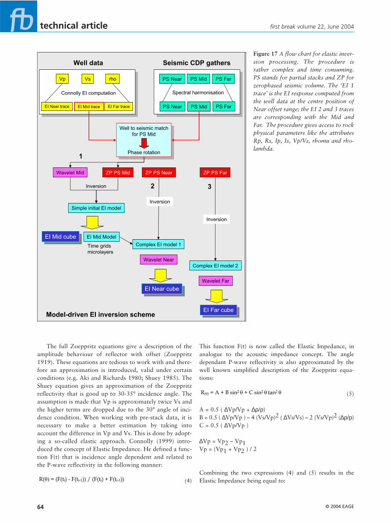
Figure 17 A flow chart for elastic inver-sion processing. The procedure israther complex and time consuming.PS stands for partial stacks and ZP forzerophased seismic volume. The ‘EI 1trace’ is the EI response computed fromthe well data at the centre position ofNear offset range; the EI 2 and 3 tracesare corresponding with the Mid andFar. The procedure gives access to rockphysical parameters like the attributesRp, Rs, Ip, Is, Vp/Vs, rhomu and rho-lambda.

© 2004 EAGE 65

technical article

(6)

Here K is a constant, that is taken to be equal to the averageof (Vs/Vp)2. Vp and Vs are expressed in m/s and the densityin gr/cm3. This type of EI computation is performed on pre-stack gathers and takes into account the changes in Vp, Vsand density as well as AVO effects. The approach is accuratefor small to moderate impedance changes. Dropping thethird term in the Shuey equation in formula (5) - which is lessaccurate, but faster - is equivalent to replace the tan2 θ bysin2 θ in the Connolly equation (6).

(7)

There are some assumptions that need to be fulfilled for thisformula (7) to be correct:■ Two term NMO approximation is correct.■ Dix's velocities are often required in the raytracing going

from the offset to the angle of incidence domain. Dix'sequation (Dix 1955) is valid for the following situation:• A layer cake geometry.• Offset is smaller than the depth of the reflector.

■ Angle of incidence θ is smaller than 30-35°, so that theShuey approximation is correct (Shuey 1985).

■ Transverse isotropic medium.■ Correctly balanced pre-stack amplitudes.■ Amplitudes are proportional to sin2 θ.

The last point implies taking out the acquisition imprint by

EI ( ) = Vp(1+ sin2 ) Vs(-8K sin2 ) (1-4K sin2 )

EI ( ) = Vp(1+ tan2 ) Vs(-8K sin2 ) (1-4K sin2 ) making the necessary source and cable corrections, sphericaldivergence correction, static and topographic corrections,prestack time migration, multiple and noise suppression,DMO, NMO and residual NMO in order to get the bestmigrated stack section. The amplitude should preserve itsproportional aspect to the original subsurface acousticimpedance contrasts or reflection coefficients. Visual inspec-tion and quality control tests play a key role in securing thatthis objective is optimally achieved.

The benefits of the elastic impedance calculations areclearly demonstrated by Figure 16. It can be easily seen thatthe larger offset angles give a better discrimination at the topof the gas reservoir. Also the Vp/Vs ratio shows a distinctbreak at this interface. The EI0 is corresponding to theacoustic impedance AI (= ρ Vp). If K = 0.25 then the EI90 =(Vp/Vs)2.

The EI seismic attribute is the basis for performing anelastic inversion similar to conventional acoustic inversionprocessing. In acoustic impedance inversion, a wavelet (shap-ing filter or cross-correlation techniques) is establishedbetween the AI trace from the well and the recorded seismictrace. In the elastic inversion, wavelets are derived for differ-ent incidence angle traces of EI(θ) and the correspondingmigrated partial stack trace. A schematic EI workflow is pre-sented in Figure 17. The diagram is rather complex and itreflects the amount of effort needed to get to the goal.

There are other formulae to approximate the EI, e.g. log-arithmic approach or also a less common non-linear function(Tarantola 1984, 1986; Pica et al. 1990). The logarithmicfunction avoids tedious exponential descriptions and is validunder the condition that K = 0.25 (Figure 18):

(8)

whereby IP = ρ Vp.

All these formulae have their own assumptions and valid-ity range. It means that the elastic inversion results are oftenonly usable in a qualitative way, as the absolute value of theinversion is not necessarily correct. For quantitative interpre-tation more processing efforts are needed, like exploiting thefull set of Zoeppritz equations.

The far offsets of these EI cubes give detailed informationon the fluid contents (Figure 19). Attributes like Rp, Rs, Ip,Is, Vp/Vs, rhomu and rholambda are easily calculated. Therhomu and lambdarho (cf Goodway et al. 1997) are derivedfrom the following expressions:

Rhomu = Is2 (9)Lambdarho = Ip2 – 2Is2 (10)

The Mu (µ) and Lambda (λ) are known as the Lame’s con-stants. Mu is the rigidity factor. The Lambda parameter is theincompressibility and contains the fluid information. Notethat it is not possible to get access to the density and veloci-

Ln (EI ( )) = Ln (I P ) + (2 Ln (Vp/Vs) - Ln (I P )) sin2


Simplified elastic impedance

Elastic impedance definition by Connolly (1999):

EI = Vp(1-tan2 ) Vs

(-8Ksin2 ) (1-4Ksin2 )

Assumption tan2 = sin2 means dropping 3rd term in Shuey approximation:

EI = Vp Vp(sin2 ) Vs

(-8Ksin2 ) (-4Ksin2 ) and Ip

= Vp

= Ip Vp(sin2 ) Vs

(-8Ksin2 ) (-4Ksin2 )

Take the logarithm of both sides and this allows to get rid of exponential notation:

Ln EI = Ln [Ip Vp(sin2 ) Vs

(-8Ksin2 ) (-4Ksin2 )]

= Ln (Ip) + Ln [Vp(sin2 ) Vs

(-8Ksin2 ) (-4Ksin2 )]

= Ln (Ip) +sin2 Ln [Vp Vs(-8K) (-4K)]

Assumption K= (Vs/Vp)2 = 0.25 , also known as a simplified elastic impedance.

Ln EI = Ln (Ip) + sin2 Ln [Vp Vs(-2) (-1)]

= Ln (Ip) + sin2 Ln (Vp /Vs2) )]

= Ln (Ip) + sin2 Ln [ (Vp2 /Vs

2) Vp)]

= Ln (Ip) + sin2 [ Ln (Vp /Vs)2 – Ln Vp)]

Ln EI = Ln (Ip) + sin2 [ Ln (Vp/Vs) – Ln (Ip)]

Figure 18 The Elastic Impedance approximation as intro-duced by Connolly (1999). The logarithmic simplification isdone under the assumption that K = 0.25. The main advan-tage is that the logarithmic EI representation avoids an awk-ward exponential notation.

© 2004 EAGE66

technical article

ty values directly for each separate layer via an inversionscheme. It is always necessary to make an estimation of theirindividual contribution to the total change in impedance ofthe various layers later on.

The calculated attributes are studied in detail and theattention is usually focused on anomalies. Well plots in zonesof interest are utilised to carry out quantitative interpretationand to perform reservoir parameter predictions. Theseparameters can also be obtained via AVO analysis, but thatcalculation is less reliable (Cambois 2000).

2. Simultaneous inversionSimultaneous inversion is calculating synthetic gathers from

perturbed P- and S-reflectivity models. The method isdescribed in detail by Ma (2002) and his article serves hereas a guide. The approach is basically model-driven. Theinversion is achieved by applying a simulated annealing tech-nique (Ma 2002). This is opposed to a genetic technique,considering the biologic evolution as a basis for the guidedMonte Carlo approach (e.g. Mallick et al. 1995).

The Aki and Richards formula (1980) gives access to theapproximate P-wave reflectivity at the various offsets in thepre-stack domain.

(11)R( ) = 0.5( ( Vp/Vp) +( / )) – 2(Vs/Vp)2 (2 ( Vs/Vs) +

( / ))sin2 + 0.5 ( Vp/Vp) tan2


Imp S LambdaRho

RhoMu Vp/Vs

EI inversion attributes

Elastic impedance sections

EI 10 degrees

EI 20 degrees

EI 30 degrees

Figure 19 The integrated approach ofan elastic inversion incorporates theAVO effect on the traces of the migrat-ed CDP gather and uses Vp and Vsinformation. Various angle dependentEI cubes and other seismic attributesare examined on anomalies that maycorrespond to lithology, porosity orfluid changes. The elastic inversionyields several seismic reservoir attrib-utes. Crossplots demonstrate their cor-relation with porefill changes.

© 2004 EAGE 67

technical article

where Vp is the average P-velocity between two uniform half-spaces, Vs is the average S-velocity and r is the average density.It can be rewritten in terms of P- and S-wave impedances:

(12)

The assumption is now made that the relative changes in(∆Vp/Vp), (∆Vs/Vs) and (∆ρ/ρ) are small and the incidenceangle θ is much less than 90°. This means that the secondorder terms can be ignored (Fatti et al. 1994):

(13)

The background Vs/Vp relationship should be known tosolve this equation. If the Vp and Vs models are not goodapproximations of the earth model, then the linear inversionwill give incorrect results. Ma (2002) proposes therefore tosubstitute the average Vs/Vp by the average Is/Ip values. ThisIs/Ip value is not coming from an a-priori model but isderived individually for each inversion iteration. Inversion is

R( ) = (1 + tan2 ( Ip/2Ip) - 8 (Vs/Vp)2 sin2 ( Is/2Is)

R(θ) = (1 + tan2 θ) (∆Ip/2Ip) - 8 (Vs/Vp)2 sin2 θ(∆Is/2Is) -(tan2 θ − 4(Vs/Vp)2 sin2 θ ) (∆ρ/2ρ)

done under the following assumptions:- The earth has approximately horizontal layers. - Each layer is described by both acoustic and shear imped-

ances. The reflection coefficients can be calculated for the n-th layerin the starting model in the following way:

(14)

(15)

(16)

These functions are utilised to compute the reflectivity at allangles in the formula above. This is convolved with thewavelet to obtain a synthetic gather. The synthetic gather iscompared with the original seismic CDP gather and the mis-fit is computed (Figure 20A). The model is subsequently per-turbed and a new comparison made to reduce the misfit. Theconvolution assumes a plane wave propagation across theboundaries of horizontally homogeneous layers and does nottake into account geometrical divergence, non-elastic absorp-tion, wavelet dispersion, transmission losses, mode conver-

Is/Ip = (Isn + Isn-1) / (Ipn + Ipn-1)

Is/2Is = (Isn – Isn-1) /(Isn + Isn-1)

Ip/2Ip = (Ipn – Ipn-1) /(Ipn + Ipn-1)


A )

B )

Modelled gathers Figure 20A Simultaneous inversion isbasically model-driven in approach.The Aki and Richards approximationof the Zoeppritz equations is used tocompute the reflectivities at differentoffsets. P- and S-wave acoustic imped-ance models are perturbed in order tocompute a new reflectivity and synthet-ic CDP gathers. These are comparedwith real seismic data and the differ-ence is minimised by a simulatedannealing technique. The advantage ofthe simultaneous inversion is that itavoids the limitation in the degree ofthe angle of incidence and the sametime model is applicable for all offsets(modified after Ma 2002).figure 20B Cross section across simul-taneous inversion results. The proposednew well location was later successfulin finding additional commercialhydrocarbons (courtesy Fugro-JasonGeoscience).

© 2004 EAGE68

technical article

sions and multiple reflections. These issues should have beenaddressed in the data pre-conditioning step.

The inversion transforms the seismic cube into reflectivi-ty cubes for different offset ranges. Cross sections and layermaps are convenient to visualize lateral changes in the inver-sion results (Figure 20B). The advantage of the simultaneousinversion is that there are few constraints on the validity ofthe computation caused by the offset angles used. A simpleinitial Vp model serves as input, summarising the expectedlow frequency variation. This approach guarantees stabilityin the end-result. A density model is constructed applyingGardner’s estimation (Gardner et al 1975) or a very simpleVp/Vs model is used (as approximation a constant value of2). A further advantage is that the same time model is appli-cable for all offset angles. The calculations are usually donefor six discrete offset angle ranges. The following attributesare computed: Vp, Vs, rhomu, lambdarho and Vp/Vs.

The two term Aki and Richards formula is frequentlywritten in a simplified form (5). It gives access to the RP andRS reflectivities for the zero offset in the following way:

Rθ = A + B sin2 θ + C sin2 tan2 θ

A = 0.5 ( ∆Vp/Vp + ∆ρ/ρ)B = 0.5 ( ∆Vp/Vp ) – 4 (Vs/Vp)2 ( ∆Vs/ Vs) – 2 (Vs/Vp)2

(∆ρ/ρ) C = 0.5 ( ∆Vp/Vp )

A is the intercept, B is the gradient in AVO analysis and C isthe AVO curvature. If Vp / Vs = 2, then for the zero degreeincidence angle (Russell et al, 2003) the two term approxi-mation is valid and :

RP 0 = A (17)

RS 0 = (A-B) /2 (18)

The density of the rock for the P- and S-wave is the same, butthe velocity contrasts change.

Also a linearised Bayesian approach has been adopted inan AVO inversion scheme (Buland and Omre 2003). TheBayes theorem exploits the conditional probability principle.The posterior solution is given by a Gaussian probabilitydensity function, whereby the calculations are based on aMonte Carlo simulation. The linearisation is made possibleby assuming weak impedance contrasts for the Zoeppritzequations. A drawback is that noise in the data has a detri-mental effect on the uncertainties in the solution.

3. Pre-stack waveform inversionThis method is based on a wave equation forward modellingalgorithm. Numerous earth models are fitted to the pre-stackresponse of the individual traces. The wave equation is runwith converted wave energy, interbed multiples, transmissionlosses and P-wave reflections (Benabentos et al. 2002, Mallick

et al. 2000). It is a computing intensive method; therefore it isoften combined with other non-linear estimation and correla-tion schemes. Neural network training is a powerful tool toconvert seismic data into pseudo well log traces (e.g. Banchsand Michelena 2002). Interval confidence calculation is donein order to adopt a more statistical approach.

The first four inversion methods described above areknown as acoustic impedance inversions. The model-driveninversion is the best suited for poor data quality surveys withlimited well control (estimated sonic, estimated density, nocheckshots?) as the seismic data itself is the basic guide forthe inversion. Elastic inversion is labour intensive and shouldonly be undertaken when a feasibility study has demonstrat-ed its benefits. A shear sonic is needed or estimated, but eventhat is not always necessary according to Cambois (2002).His suggested fluid factor basically boils down to the behav-iour of the far offset stack.

A word of cautionAs a word of warning: ‘Seismic inversion is not a uniqueprocess’. There are several AI models that generate similarsynthetic traces when convolved with the wavelet. The num-ber of possible solutions is significantly reduced by puttingconstraints on the modelling and, in doing so, a most plausi-ble scenario is retained (Veeken et al. 2002, Da Silva et al., inprep). The support of other investigation techniques, likeAVO analysis and forward modelling, increases the confi-dence in the inversion results. Even a negative correlation isimportant information as it results in an increase of the riskattached to the prospect. It may sound a bit controversial,but ultimately it will reduce the drilling risk on the well pro-posals because of the better ranking criteria.

Seismic velocities are sensitive to the presence of gas in arock sequence. A 5-10% gas saturation has already a tremen-dous impact on the seismic response. It will lead to AVO andAI anomalies, but these are non-commercial. The extent ofthe mapped anomalies should therefore always be treatedwith some care. AVO and inversion anomalies are likelyrelated to the maximum distribution of hydrocarbons.

Seismic inversion depends heavily on the proper integra-tion of well data. Incorporation of anisotropy effects in theinversion scheme will improve the quality of the output data(Rowbotham et al. 2003). This is especially important whendealing with deviated holes.

Seismic inversion is gradually becoming a routine pro-cessing step in field development studies as well as forexploration purposes. Even time lapse inversions are nowconducted (Gluck et al. 2000, Oldenziel 2003). The AIattribute is gradually replacing the normal amplitude seis-mic representation as inversion is becoming an integral partof the reservoir characterisation workflow (cf Latimer et al.2000, Van Riel 2000). The positive track record of case his-tories clearly demonstrates the added value of this type ofseismic analysis.


© 2004 EAGE 69

technical article

ConclusionsInversion replaces the seismic signal by a blocky impedanceresponse. Various seismic inversion schemes are available,each having their own advantages. Input data conditioning isan important step when quantitative interpretation is theultimate goal. Model-driven inversion is robust, even whendealing with poor data sets. A true 3D approach stabilisesthe output. The probabilistic method quantifies uncertaintiesin the geological model and incorporates these in the endresults. The shared earth model is suited as input to reservoirsimulation packages. The pre-stack approach exploits AVOeffects present in the seismic dataset. All of these methodshave their own restrictions and limitations. Feasibility andsynthetic modelling studies are recommended before startingan inversion and/or AVO project.

There is a trade-off between work involved / cost / timeand quality of the end product. Seismic inversion is not aunique process, i.e. there is not a single solution to the givenproblem. In other words: several AI or EI models may equal-ly well explain the same seismic response. Numerous studieshave already proven the added value of inversion processingfor better definition of prospects and leads, improved DHIdetection, delineation of sweet spots with better porosity andpermeability characteristics. All these aspects allow optimisa-tion of field development plans with improved volumetricestimations and make more reliable economic forecasts pos-sible.

AcknowledgementsWe are indebted to CGG, CMG, Pemex and JasonGeoscience companies for granting permission to use theirdata. We thank our immediate colleagues for sharing theirworking ideas. In particular we want to thank Dr E. Mendez,M. Rauch-Davies, H. Bernal, G. Velasquez, A. Marhx, J.Camara, N. Van Couvering, R. Walia, J. Helgesen, M.Querne, Y. Lafet, J.M. Michel, C. Pinson, S. Addy, R.Martinez, JL. Gelot and P. Van Riel for their contributions.The comments of the reviewers have been highly appreciat-ed. Special thanks is given to Dr M. Bacon for his construc-tive remarks.

ReferencesAki, K. and Richards, P.G. [1980] Quantitative seismology, the-ory and methods. Freeman, San Francisco, 557.Ajlani, G., Al Kaabi, M. and Suwainna, O. [2003] Comparativeanalysis ( CASP): a proposal for quantifying seismic data process-ing. The Leading Edge, 22, 1, 46-48.Banchs, R. E. and Michelena, R.J. [2002] From 3D seismic attrib-utes to pseudo-well-log volumes using neural networks: practicalconsiderations. The Leading Edge, 21, 10, 996-1001.Benabentos, M., Mallick, S., Sigismondi, M. and Soldo, J. [2002]Seismic reservoir description using hybrid seismic inversion: a 3Dcase study from the Maria Ines Oeste Field, Argentina. TheLeading Edge, 21, 10, 1002-1008. Buland, A. and Omre, H. [2003] Bayesian linearized AVO inver-

sion. Geophysics, 68, 1, 185–198.Cambois, G. [2000] AVO inversion and elastic impedance.Expanded abstracts, 70th SEG Annual Meeting, Calgary, 1-4. Castagna, J.P. and Backus, M.M. [1993] Offset dependent reflec-tivity – Theory and practice of AVO analysis. SEG, Tulsa,Investigations in Geophysics 8, 348.Connolly, P. [1999] Elastic impedance, The Leading Edge, 18, 4,438-452.Cook, D.A. and Sneider, W.A. [1983] Generalized linear inversionof reflection seismic data. Geophysics, 48, 665-676.Cosentino, L. [2001] Integrated reservoir studies. Technip, Paris,310.Coulon, J.P., Duboz, P. and Lafet, Y. [2000] Moving from seismicto layered impedance cube and porosity prediction in the Natih Emember. GeoArabia, 5, 1, 72-73.Da Silva, M., Rauch-Davies, M., Soto Cuervo, A. and Veeken, P.in prep. , Pre- and post-stack attributes for enhancing productionfrom Cocuite gas reservoirs. 66th EAGE Annual Conference,Paris [2004]Da Silva, M., Rauch-Davies, M., Soto Cuervo, A. and Veeken, P.in prep. , Data conditioning for a combined inversion and AVOstudy. 66th EAGE Annual Conference, Paris, [2004]Dix, C.H. [1955] Seismic velocities from surface measurements.Geophysics, 20, 68-86.Duboz, P., Lafet, Y. and Mougenot, D. [1998] Moving to layeredimpedance cube: advantages of 3D stratigraphic inversion. FirstBreak, 17, 9, 311-318.Dubrule, O. [2003] Geostatistics for seismic data integration inearth models. EAGE Distinguished Instructor Series 6, 282.Dutta, N.C. [2002] Geopressure prediction using seismic data:Current status and the road ahead. Geophysics, 67, 6, 2012-2041.Fabre, N., Gluck, S., Guillaume, P. and Lafet, Y. [1989] Robustmultichannel strati-graphic inversion of stacked seismic traces,59th Annual Meeting SEG, 943. Fatti, J.L., Smith, G.C., Vail, P.J., Strauss, P.J. and Levitt, P.R.[1994] Detection of gas in sandstone reservoirs using AVO analy-sis.: A 3-D seismic case history using the Geostack technique.Geophysics, 59, 1362-1376.Faust, L.Y. [1951] Seismic velocity as a function of depth and geo-logic time. Geophysics, 16, 192-206.Faust, L. Y. [1953] A velocity function including lithologic varia-tions. Geophysics, 18, 271-287.Gardner, G.H.F., Gardner, L.W. and Gregory, A.R. [1974]Formation velocity and density - The diagnostic basics for strati-graphic traps, Geophysics, 39, 770-780.Gluck, S., Juve, E. and Lafet, Y. [1997] High resolution imped-ance layering through 3D stratigraphic inversion of post stackseismic data. The Leading Edge, 16, 1309- 1315.Gluck, S., Deschizeaux, B., Mignot, A. Pinson and Huguet, F.[2000] Time-lapse impedance inversion of post-stack seismic data.Expanded abstracts, 70th Annual Meeting SEG, Calgary, 1509-1512. Goffe, W.L., Ferrier, G.D. and Rodgers, J. [1994] Global optimi-sation of statistical functions with simulated annealing. Journal of


© 2004 EAGE70

technical article

Econometrics, 60, 65-100.Goodway, W., Chen, T. and Downton, J. [1997] Improved AVOfluid detection and lithology determination using Lame’s petro-physical parameters: LambdaRho, MuRho and Lambda/Mufluid stack from P and S inversions. Canadian Society ofExploration Geophysicists, Abstracts, 148-151. Haas, A. and Dubrule, O. [1994] Geostatistical inversion – asequential method of stochastic reservoir modelling constrainedby seismic data. First Break, 12 , 11, 561-569.Hardage, B.A., [1985] Vertical seismic profiling - a measurementthat transfers geology to geophysics: in Berg O.R. and WoolvertonD.G. (eds) [1985,] Seismic stratigraphy II: an integrated approachto hydrocarbon exploration, AAPG Memoir 39, AAPG, Tulsa,13-34.Helland-Hansen, D., Magnus, I., Edvardsen, A., and Hansen, E.[1997] Seismic inversion for reservoir characterisation and newwell planning in the Snorre field. The Leading Edge, 16, 3, 269-273.Lancaster, S. and Whitcombe, D. [2000] Fast track "coloured"inversion. Expanded abstracts, 70th SEG Annual Meeting,Calgary, 1572-1575. Latimer, R.B., Davison, R. and Van Riel, P. [2000] Interpreter'sguide to understanding and working with seismic derived acousticimpedance data. The Leading Edge, 19, 3, 242-256. Lindseth, R. [1979] Synthetic sonic logs - a process for strati-graphic interpretation. Geophysics, 44, 3-26.Ma, X. [2002] Simultaneous inversion of prestack seismic datafor rock properties using simulated annealing. Geophysics, 67,1877-1885.Mallick, S. [1995] Model-based inversion of amplitude variationswith offset data using a genetic algorithm. Geophysiscs, 60, 939-954.Mallick, S., Lauve, J. and Ahmad, R. [2000] Hybrid seismic inver-sion: A reconnaissance tool for deep water exploration. TheLeading Edge, 19, 38-43.Mari, J.L., Glangeaud, F. and Coppens, F. [1999] Signal process-ing for geologists and geophysicists. Editions Technip, Paris, 480 Metropolis, N., Rosenbluth, A., Rosenbluth, M., Teller, M., andTeller, E. [1953] Equation of state calculations by fast computingmachines. Journal Chem Phys, 21, 1087-1092. Oldenziel, T. [2003] Time lapse seismic within reservoir engineer-ing. Thesis, Delft University of Technology, 204.Onderwater, J., Wams, J. and Potters, H. [1996] Geophysics inOman. GeoArabia, 1, 2, 299-324.Pendrel, J., Stewart, R.R. and Van Riel, P. [1998] Interpreting sandchannels from 3C-3D seismic inversion. Expanded Abstracts,71th SEG Annual Meeting, 1588-1591.Pica, A., Diet, J. and Tarantola, A. [1990] Non linear inversion ofseismic reflection data in a laterally invariant medium.Geophysics, 55, 284-292.Ronghe, S. and Surarat, K. [2002] Acoustic impedance interpre-tation for sand distribution adjacent to a rift boundary fault,Suphan basin, Thailand. AAPG Bulletin, 86, 10, 1753-1771.Rowbotham, P., Marion, D., Eden, R., Williamson, P., Lamy, P.and Swaby, P. [2003] The implications of anisotropy for seismic

impedance inversion. First Break, 21, 53-57.Russell, B.H., Hedlin, K., Hilterman, F.J. and Lines, L.R. [2003]Fluid property discrimination with AVO: A Biot-Gassmann per-spective. Geophysics, 68, 1, 29-39.Sheriff, R.E. [2002] Encyclopedic dictionary of exploration geo-physics. SEG, Tulsa, 429. Shuey, R.T. [1985] A simplification of the Zoeppritz equations.Geophysics, 50, 609-614.Stewart, R.R., Gaiser, J.E., Brown, R. and Lawton, D.C. [2003]Converted-wave seismic exploration: applications. Geophysics,68, 1, 40-57.Sylta, O. and Krokstad, W. [2003] Estimation of oil and gas col-umn heights in prospects using probabilistic basin modellingmethods. Petroleum Geoscience, 9, No. 3, 243-254.Tarantola, A. [1984] Inversion of seismic reflection data in theacoustic approximation. Geophysics, 49, 1259–1266.Tarantola, A. [1986] A strategy for non linear elastic inversion ofseismic reflections data. Geophysics, 51, 1893-1903.Torres-Verdin, C., Victoria, M., Merletti, G. and Pendrel, J.[1999] Trace-based and geostatistical inversion of 3-D seismicdata for thin sand delineation: An application in San Jorge Basin,Argentina. The Leading Edge, 18, 9 , 1070-1077.Trad, D., Ulrych, T. and Sacchi, M. [2003] Latest views of thesparse Radon Transform. Geophysics, 68, 1, 386-399.Van der Laan, J. and Pendrel, J. [2001] Geostatistical simulationof porosity and risk in a Swan Hills reef. Expanded abstracts,71th SEG Annual Meeting, 1588-1591.Van Riel, P., [2000] The past, present and future of reservoir char-acterization. The Leading Edge, 19, 8, 878-881.Vazquez, R., Mendoza, A., Lopez, A., Linares, M. and Bernal, H.[1997] 3-D seismic role in the integral study of the Arcabuz-Culebra field, Mexico. The Leading Edge, 16, 12, 1763-1766.Veeken, P.C.H., (in prep.), Seismic stratigraphy, basin analysis andreservoir characterisation. Elsevier, Amsterdam, 350.Veeken, P.C.H., Rauch, M., Gallardo, R., Guzman, E. and Vila, R.Villasenor [2002] Seismic inversion of the Fortuna National 3Dsurvey, Tabasco, Mexico. First Break, 20, 5, 287-294. Velzeboer, C.J. [1981] The theoretical seismic reflection responseof sedimentary sequences. Geophysics, 46, 843-853.Walden, A.T. and Hosken, J.W.J. [1985] An investigation of thespectral properties of primary reflection coefficients. GeophysicalProspecting, 33, 400-435.Weber, K.J. and Van Geuns, L.C. [1990] Framework for con-structing clastic reservoir simulation models. Journal of PetroleumTechnology, 42, 10, 1248-1297.White, R. and Simm, R. [2003] Tutorial: Good practice in wellties. First Break, 21, 10, 75-83. Yilmaz, O. [1987] Seismic data processing, Society ofExploration Geophysicists, Investigations in geophysics, 2, Tulsa,SEG, 526.Yilmaz, O. [2001] Seismic data analysis, Volume 1 and 2. Societyof Exploration Geophysicists, Investigations in geophysics, 10,Tulsa, SEG, 2027.Zoeppritz, K. [1919] On the reflection and propagation of seis-mic waves, Erdbebenwellen VIIB, Gottinger Nachrichten I, 66-84.


Seismic inversion methods and some of their … · Introduction The interest in seismic inversion...

Documents

Transcript of Seismic inversion methods and some of their … · Introduction The interest in seismic inversion...