Seismic deconvolution by atomic decomposition: a parametric approach

with sparseness constraints

Felix J. Herrmann

August 6, 2004

Abstract

In this paper an alternative approach to the blind seismic deconvolution problem is presented that aims for two

goals namely recovering the location and relative strength of seismic reflectors, possibly with super-localization,

as well as obtaining detailed parametric characterizations for the reflectors. We hope to accomplish these goals

by decomposing seismic data into a redundant dictionary of parameterized waveforms designed to closely match

the properties of reflection events associated with sedimentary records. In particular, our method allows for

highly intermittent non-Gaussian records yielding a reflectivity that can no longer be described by a stationary

random process or by a spike train. Instead, we propose a reflector parameterization that not only recovers the

reflector’s location and relative strength but which also captures reflector attributes such as its local scaling,

sharpness and instantaneous phase-delay. The first set of parameters delineates the stratigraphy whereas the

second provides information on the lithology. As a consequence of the redundant parameterization, finding the

matching waveforms from the dictionary involves the solution of an ill-posed problem. Two complementary

sparseness-imposing methods Matching and Basis Pursuit are compared for our dictionary and applied to seismic

data.

1 Introduction

In seismic imaging we are interested in obtaining information on the nature of transitions in the subsurface from

seismic data collected at the surface. Not only do seismic waves reflect at these transitions but they also constitute

1

regions of geologic [Herrmann, 2001b, Herrmann et al., 2001a], geophysical and rock-physical interest [Herrmann and

Bernabe, 2004]. Seismic imaging roughly consists of two main steps. First, kinematic effects of the wave propagation

are removed by a process called migration, which corresponds to applying the adjoint of the linearized forward-

scattering operator to seismic data [Brandsberg-Dahl and de Hoop, 2003, Kuhl and Sacchi, 2003, ten Kroode et al.,

1998]. Remaining source-function [Levy et al., 1988, Oldenburg et al., 1981, 1988, Robinson, 1957, Scheuer, 81, Ulrych

and Walker, 1982], imaging [Hu et al., 2001] and propagation influences are removed during a second step, which

is designed to improve the resolution as well as amplitude characteristics of the image. Without loss of generality,

our main focus is the elimination of the unknown source-function, which is generally referred as the seismic blind

deconvolution problem.

Seismic deconvolution is a classical example of an ill-posed problem since it involves the removal of a “blurring”

by the source-function. Hence, additional assumptions have to made regarding the imaged seismic reflectivity (the

model) and the blurring kernel (the seismic wavelet). Typically, these assumptions impose certain stochastic sta-

tionarity conditions on the reflectivity, minimum-phase on the wavelet, or minimum structure on the reflectivity in

conjunction with certain smoothness conditions on the wavelet.

Almost half a century ago, Robinson [1957] solved the blind deconvolution problem by imposing stochastic

homogeneity and Gaussianity on the noise as well as on the reflectivity, yielding optimal Wiener shrinkage estimators

[Mallat, 1997, Robinson, 1957]. These shrinkage estimators correspond to a regularized spectral devision. Given the

ambitious goals of this paper, the stochastic homogeneity and Gaussianity conditions for the reflectivity may prove to

be too imposing, even though recent extensions [Saggaf and Robinson, 2000] of the theory to include anti-correlated

reflectivity have certainly been encouraging. However, our main goal is to truly honor the ubigious intermittent and

non-Gaussian behavior displayed by sedimentary records [Herrmann, 1998, 2003a, Herrmann et al., 2001a, Muller

et al., 1992, Saucier and Muller, 1993] in the blind deconvolution problem.

There have been several attempts by Levy et al. [1988], Oldenburg et al. [1981, 1988], Scheuer [81], Ulrych and

Walker [1982] and later by [Sacchi et al., 1994] to incorporate the notion of intermittency in deconvolution by so-

called minimum structure/entropy approaches that impose a certain spikyness or sparseness on the reflectivity. Even

though, the assumption of spike trains for the reflectivity is perhaps too much of a simplification, it does capture

the intermittency, which is a telltale signs of multi-fractal behavior [Herrmann, 1998, 2003a, Herrmann et al., 2001a,

2

Muller et al., 1992, Saucier and Muller, 1993]. Minimum structure jointly with regularity and wigglyness conditions

on the source-function [Oldenburg et al., 1981] have led to a wealth of highly successful deconvolution schemes. These

approaches form the main motivation for our work.

The basic idea is that we aim to solve the blind deconvolution problem by decomposing a seismic reflection trace

with respect to a redundant dictionary of parameterized seismic waveforms that are designed to sparsely represent

the seismic reflectivity and hence the Earth model [Herrmann, 2003a,b, Herrmann and de Hoop, 2002]. A major

difference between this approach, which can also found in Trad [2001]’s work on sparse Radon and earlier work,

is that we try to accomplish sparseness incorporating a wider range of possible source signatures and in particular

transition types [Herrmann, 2001b, Herrmann et al., 2001a]. Essentially, our approach is a departure from the classic

assumption of a spike train for the reflection density towards a reflector model whose parameterization contains

detailed information on the reflector’s abruptness, scaling and instantaneous phase-delay properties. Our choice of

parameterization is motivated by (i) observed scaling properties from sedimentary records [Herrmann, 1998]; (ii) the

mathematical relevance of the local regularity Herrmann [2001b, 2003a], (iii) the success of classical complex-trace

attributes [Harms and Tackenberg, 1972, Payton, 1977] and their recent extensions using wavelets and Matching

Pursuit [Dessing, 1997, Herrmann, 2001a, Steeghs, 1997, Verhelst, 2000] and (iv) the geological [Herrmann et al.,

2001a] and rock-physical [Herrmann and Bernabe, 2004] relevance of the transition order and phase characteristics.

These latter properties can be interpreted as a modern version of the complex trace attributes known within seismic

stratigraphy [Harms and Tackenberg, 1972, Payton, 1977]. Wapenaar [1999] discusses the influence of the transition

order on the amplitute-variation-with-angle, which is a topic of current interest but outside the scope of this paper.

Two main issues will be addressed in this paper: (i) the construction of the appropriate dictionary that accounts

for subtle sharpness and instantaneous-phase changes along major unconformities and (ii) the solution of the blind

deconvolution problem addressing issues such as non-uniqueness and super-resolution [Chen et al., 2001]. Because of

the redundancy of the dictionary, the solution of the blind deconvolution problem involves the solution of a highly

underdetermined inverse problem. Systematic comparisons will be made between two different solution strategies:

Matching and Basis Pursuit [Chen et al., 2001, Mallat, 1997]. Both strategies aim for a sparse representation of the

reflectivity who’s parameterized elements not only contain information on the location of the reflectors, i.e. yielding

a ”spiky decon”, but also on reflector details such as its scale, instantaneous phase and sharpness.

3

The paper is organized as follows. First, we introduce the seismic deconvolution problem in its general form

and discuss some known strategies for its solution. We then proceed by introducing our solution strategy based on

an atomic decomposition with respect to a dictionary of parameterized waveforms. In the construction, particular

attention will be paid to defining transitions that not only continuously interpolate between zero- and first-order

transitions but which also allow for a more precise determination of the reflector’s instantaneous phase-delay char-

acteristics. In this way, we aim to resolve the issue of π/2-phase changes along major reflectors as can be observed

in Fig. 1, which contains an example of Matching Pursuit applied to an imaged seismic section. We discuss how

source-functions and seismic reflectors can both be represented by Fractional Splines [Unser and Blu, 2000] that

allow for a precise control over the regularity, wiggliness and instantaneous phase characteristics. We also show that

these splines lead to a fast implementation by recursive filter banks [Mallat, 1997, Unser and Blu, 2000]. Given the

construction of the dictionary, we subsequently review two different strategies to select the appropriate waveforms

from the dictionary. It is shown that under certain conditions these waveforms yield a sparse representation for the

reflection data which solves the deconvolution problem. By means of a series of examples, we compare the different

merits and shortcoming of the greedy search strategy Matching Pursuit and the global constraint optimization of

Basis Pursuit.

2 The deconvolution and characterization problem

2.1 Seismic deconvolution

Seismic deconvolution commits itself to removing the effects of a “blurring” kernel on the seismic image. With

the seismic image, we generally refer to an image obtained by operating the adjoint of the scattering operator on

noisy seismic data. The blurring kernel, known as the seimic wavelet, contains the effects of the source-function,

illumination and dispersion and can mathematically be represented by a generalized convolution operator given by

d = Km + n. (1)

The model, m, represents the reflectivity and is linearly related to the observed seismic reflection trace, d, by the

kernel K. n is taken to be a white Gaussian noise process representing measurement errors as well as possible

shortcomings of the operator K to model seismic data. With a slight abuse of notation we will replace the operator,

4

model and data by a discrete matrix and vectors. In addition, the matrix K is assumed to be Toeplitz, yielding a

convolution, while the noise is taken to be a realization of a Gaussian pseudo-random generator, yielding discrete

white noise.

Given K, the model can be inverted from noisy data by solving the following variational problem

m : minm

12‖d−Km‖22 + νJ(m), (2)

where J(m) is a ν-weighted global penalty-functional [Vogel, 2002], which contains a priori information on the model.

For quadratic penalty-functions, Eq. 2 corresponds to a Tikhonov-regularization [Vogel, 2002], where the penalty

term J(m) = ‖Lm‖2 with L a (sharpening) operator defines the Covariance operator (C = (L∗L−1) for the model.

This formalism forms the basis of many least-squares inversion techniques and allows for a colored reflectivity model

[Robinson, 1957, Saggaf and Robinson, 2000].

Because L2-norms have a tendency to spread the energy, quadratic penalty-functionals do not preserve or obtain

sparseness. L1- or entropy-norms, on the other hand, preserve sparseness and this explains the current resurgence

of sparseness-constrained inversion techniques [Kuhl and Sacchi, 2003, Schonewille and Duijndam, 2001], which has

led to successful spike-train solutions of the deconvolution problem. In this paper, we allow for a more general types

of transitions that go beyond Earth models that consist of isolated jump-discontinuities.

2.2 Atomic deconvolution

To incorporate a wide class of different types of source functions and spatially varying transitions, we choose for

an adaptive representation for the individual waveforms in seismic records. We adopt a localized matched filtering

technique, where data is composed from parameterized waveforms designed to represent the convolutional action of

the source-function with the different transition types. Given this dictionary, seismic data can sparsely be represented

by a superposition over a limited number of atoms that reside in the columns of a matrix that represents the dictionary,

i.e.

d = Φc. (3)

In this expression, c represents the sparse coefficient vector and Φ the dictionary. Comparison with Eq. 1 shows that

the dictionary matrix and coefficient vector replace the convolution kernel, K, and the model, m, respectively. The

5

dictionary Φ contains the parameterized waveforms Φ = {gλ[k]}0≤k<n, λ∈Λ as its columns with λ the index for the

parameterization of each atom, Λ the index-set and n the number of data samples in the seismic record.

The question is now how to find the coefficient vector given seismic data. To answer this question, we proceed

by introducing two alternative strategies that are aimed at finding a sparse representation for the coefficient vector

c. When these coefficients are found, the blind deconvolution problem is solved because these coefficients are a

representation for the reflectivity. In addition, the coefficients provides information on the location and relative

strengths of the reflectors. Because of the large redundancy in the dictionary, i.e. Φ is a rectangular n × p-matrix

(with p the number of columns, i.e. total number of entries in the index-set Λ), the coefficient vector c can not

straightforwardly estimated from seismic recordings. We compare Matching Pursuit (MP) [Mallat, 1997] and Basis

Pursuit (BP) [Chen et al., 2001] as possible solution techniques, which either follow a greedy search strategy that

iteratively selects the best matching atoms, or which solves the problem by global optimization which corresponds

to solving

c : minc

12‖d− Φc‖22 + ν‖c‖1. (4)

This optimization problem minimizes the L2-difference between data and model subject to an additional L1-penalty

term that enforces sparseness on the coefficient vector. Both strategies should allow for the removal of incoherent noise

and provide detailed information on the location, relative strength, scale, instantaneous phase-delay and sharpness

of the reflectors. Before going into detail on how to compute the coefficients, we first describe the construction of

the appropriate dictionary.

3 Construction of the dictionary

As in any matched-filter approach, the success of the filter depends on how well the filter correlates with the signal.

The situation for our atomic-decomposition approach is not different, except that we use highly localized waveforms

that are able to adapt themselves to local features in seismic data. The main challenge is not only to find the

appropriate parameterization for the combined action of the source-function and reflectors but also to develop a

fast numerical implementation, based on wavelet transform filter banks. First, we introduce parameterizations for

the source-function and reflector models, followed by an in-depth discussion on the construction of a dictionary

implemented by fast discrete wavelet transforms.

6

3.1 Parameterization of the source-function

To construct the dictionary, assumptions are needed regarding the seismic source wavelet. For our purpose, it

suffices to restrict the source-function’s smoothness and wiggliness. The first condition controls the decay of the

Fourier spectrum for frequencies going to infinity whereas the second condition rules the differentiability of the

Fourier transform at zero frequency. Both conditions combined, determine the details of the frequency content of

the source-function. Mathematically, these conditions correspond to

• imposing∫|ϕ|(ω)|ω|αdω <∞, which means that the wavelet is α-times continuously differentiable, i.e. ϕ ∈ Cα.

• requiring the wavelet ϕ to be orthogonal with respect to some finite-order polynomial,

∫ +∞

−∞tqϕ(x)dx = 0 ⇐⇒ <{∂q

ωϕ}ω=0 = 0 for 0 ≤ q < M. (5)

The first condition limits the high-frequency content by setting the asymptotic decay rate for high frequencies. The

second condition defines the number of vanishing moments and is related to the wavelet’s wiggliness. This latter

property defines the number of derivatives of a smoothing function that define the wavelet. These derivatives are

essential for the definition of wavelets within wavelet theory and can also be found in independent work by Oldenburg

et al. [1981].

3.2 Parametrized Reflector Model

Motivated by empirical findings that the Earth’s subsurface behaves like a multifractal – it is a medium that consists

of accumulations of varying order singularities – we propose a parametric representation for the subsurface that

consists of a superposition of singularities of the type [Herrmann, 2001b, 2003a, Herrmann et al., 2001b, Herrmann,

1997]:

χα+(x) =

0 x ≤ 0

xα

Γ(α+1) x > 0

, χα−(x) =

0 x ≥ 0

xα

Γ(α+1) x < 0

(6)

for causal (+) and anti-causal (−) transitions and

χα∗ (x) =

|x|α

−2 sin(π/2α)Γ(α+1) α not even

x2n

(−1)1+nπΓ(α+1) α = 2n even

(7)

7

for symmetric cusp transitions. The Γ is the Gamma function. In this model, the zero- and first-order discontinuities

often used to model seismic reflectors are replaced by α-order fractional splines [Unser and Blu, 2000]. Given these

splines, we are able to represent the “layered” Earth by a superposition of Fractional Splines of varying order. This

superposition leads to what we will call a Multi-fractional Spline representation [Herrmann, 2003a], consisting of a

weighted combination of different Fractional Splines

f(x) ,∑n∈N

cnχαn±, ∗.(x− xn) (8)

By setting α = 0, we obtain after differentiation the well-known spike train for the reflection density, which consists

of a series of delta-Dirac distributions

r(x) =∑n∈N

cnδ(x− xn). (9)

For varying α, we obtain

r(x) =∑n∈N

cnαχαn−1±, ∗ (x− xn) (10)

with cnα constants that depend on the order of the Fractional Splines. By construction, the transition-orders are

allowed to vary, a behavior consistent with that of multi-fractals, where the local regularity given by the same α,

changes discontinuously from position to position. For α < 1, the above derivative of Eq. 8 is taken in the sense of

distributions.

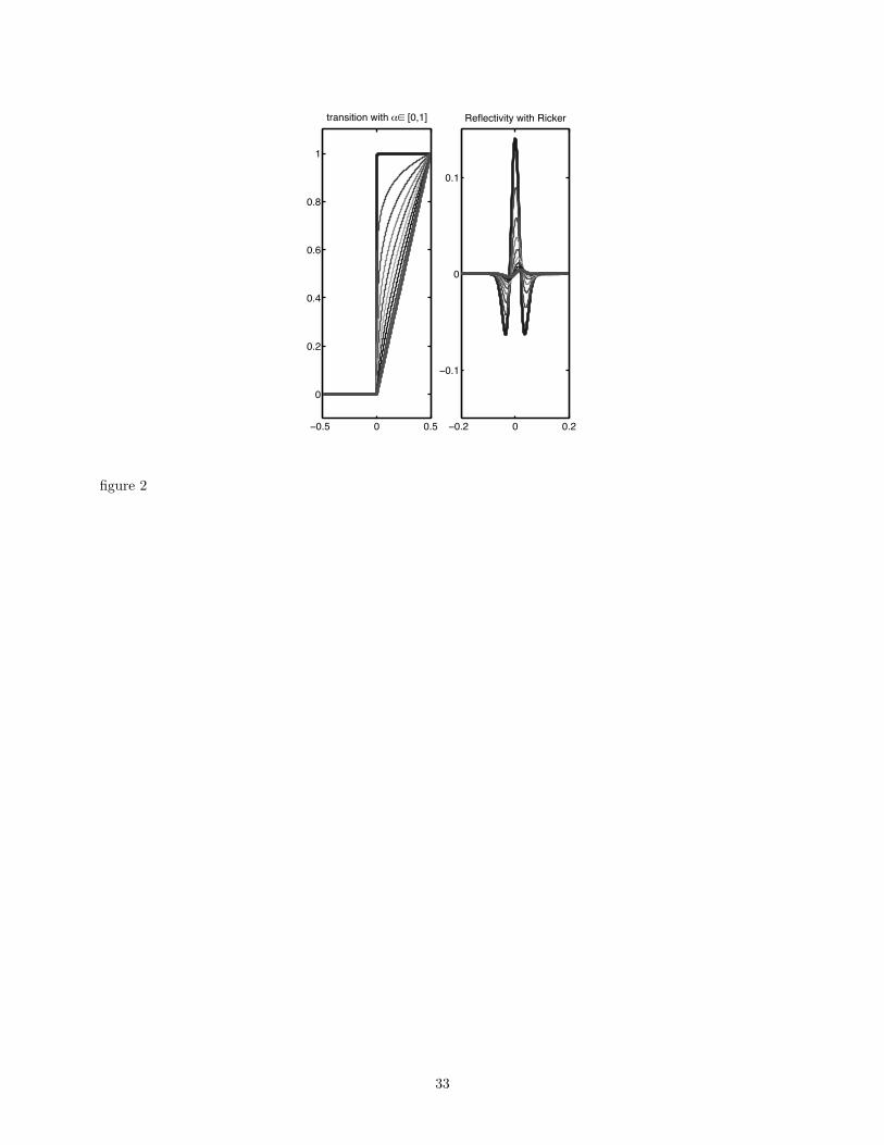
Fig. 2 illustrates how changes in the order α influence the transition sharpness and the amplitude/phase charac-

teristics of the induced reflection response for a Ricker wavelet. The response is given by

d(x) = (r ∗ ϕ) (x), (11)

with ϕ(x) the seismic wavelet and r given by Eq. 10. For non-integer α, the transitions have a distinct phase behavior

as demonstrated in Fig. 3, where both the causal (+) and anti-causal (−) transitions are shown together with their

induced waveforms.

Transitions with 0 < α < 1 continuously interpolate between step- (α = 0) and ramp-discontinuities (α = 1),

while the extension to α < 0 yields transitions that, e.g. for α = −1, can be interpreted as a thin layer which acts as

a differentiator for the low frequencies. For α > 0, the transitions defined in Eq.’s 6 and 7 act as α-order fractional

integrators and display the following scale-invariance (irrespective of their instantaneous phase)

χα(σx) = σαχα(x). (12)

8

Despite these very useful scaling, regularity and sharpness properties, Fractional Splines are not local and lack a

fast numerical implementation. In the next section, we will shift our attention to the definition of fast numerical

implementations for orthogonal B-splines that share the same regularity properties but which are local and allow for

a more precise characterization of the instantaneous phase.

3.3 Fractional Spline Wavelet dictionary

For the solution of our deconvolution problem, dictionaries with localized waveforms are necessary with prescribed

regularity, wigglyness, decay and phase-delay properties. To battle the fact that finding the appropriate waveforms

from the dictionary is a NP-hard problem [Mallat, 1997], we need a fast numerical implementation. To ensure

translation invariance, non-decimated stationary wavelet transforms [Coifman and Donoho, 1995] are used, which

are computed by a filter bank whose Quadrature Mirror Filters (QMF’s) are defined by orthonormal generalized

Fractional Splines. These splines offer optimal flexibility with respect to prescribed regularity and phase-delay

characteristics. The main steps in the construction of the dictionary are described next.

3.3.1 B-splines and generalized B-splines

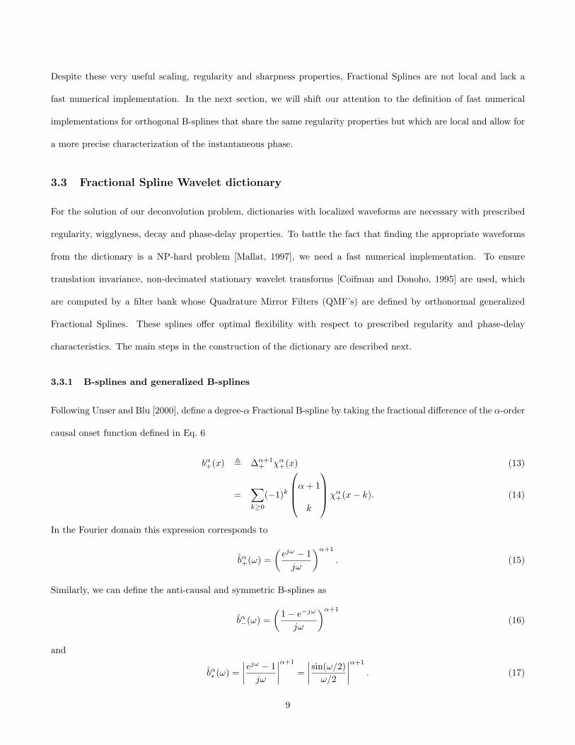
Following Unser and Blu [2000], define a degree-α Fractional B-spline by taking the fractional difference of the α-order

causal onset function defined in Eq. 6

bα+(x) , ∆α+1+ χα

+(x) (13)

=∑k≥0

(−1)k

α+ 1

k

χα+(x− k). (14)

In the Fourier domain this expression corresponds to

bα+(ω) =(ejω − 1jω

)α+1

. (15)

Similarly, we can define the anti-causal and symmetric B-splines as

bα−(ω) =(

1− e−jω

jω

)α+1

(16)

and

bα∗ (ω) =∣∣∣∣ejω − 1

jω

∣∣∣∣α+1

=∣∣∣∣ sin(ω/2)

ω/2

∣∣∣∣α+1

. (17)

9

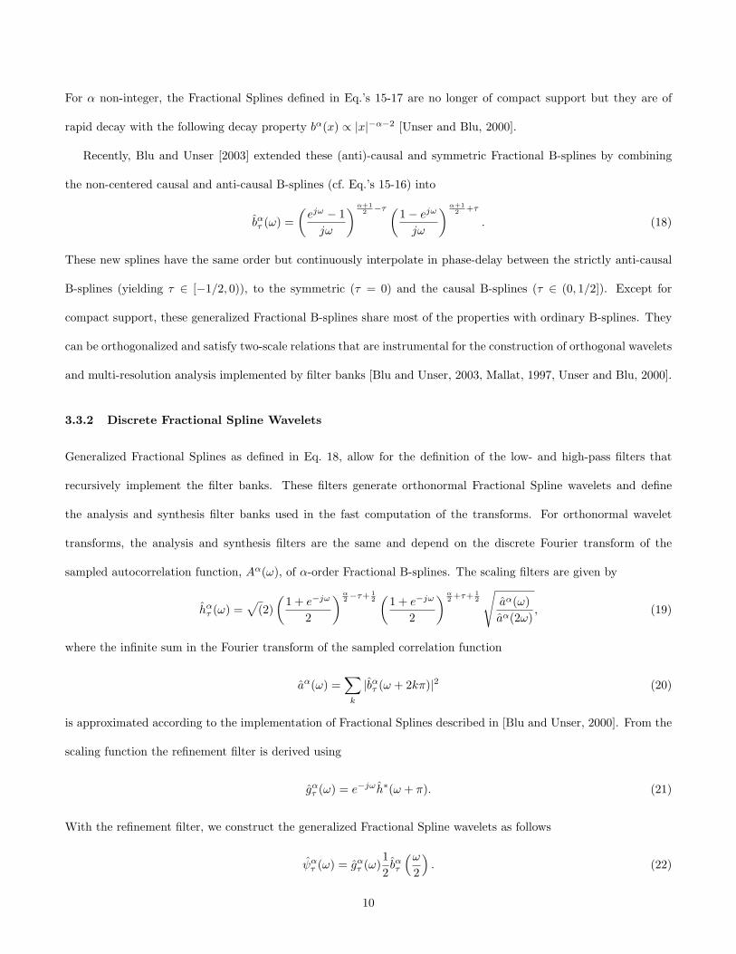
For α non-integer, the Fractional Splines defined in Eq.’s 15-17 are no longer of compact support but they are of

rapid decay with the following decay property bα(x) ∝ |x|−α−2 [Unser and Blu, 2000].

Recently, Blu and Unser [2003] extended these (anti)-causal and symmetric Fractional B-splines by combining

the non-centered causal and anti-causal B-splines (cf. Eq.’s 15-16) into

bατ (ω) =(ejω − 1jω

)α+12 −τ (

1− ejω

jω

)α+12 +τ

. (18)

These new splines have the same order but continuously interpolate in phase-delay between the strictly anti-causal

B-splines (yielding τ ∈ [−1/2, 0)), to the symmetric (τ = 0) and the causal B-splines (τ ∈ (0, 1/2]). Except for

compact support, these generalized Fractional B-splines share most of the properties with ordinary B-splines. They

can be orthogonalized and satisfy two-scale relations that are instrumental for the construction of orthogonal wavelets

and multi-resolution analysis implemented by filter banks [Blu and Unser, 2003, Mallat, 1997, Unser and Blu, 2000].

3.3.2 Discrete Fractional Spline Wavelets

Generalized Fractional Splines as defined in Eq. 18, allow for the definition of the low- and high-pass filters that

recursively implement the filter banks. These filters generate orthonormal Fractional Spline wavelets and define

the analysis and synthesis filter banks used in the fast computation of the transforms. For orthonormal wavelet

transforms, the analysis and synthesis filters are the same and depend on the discrete Fourier transform of the

sampled autocorrelation function, Aα(ω), of α-order Fractional B-splines. The scaling filters are given by

hατ (ω) =

√(2)

(1 + e−jω

2

)α2−τ+ 1

2(

1 + e−jω

2

)α2 +τ+ 1

2

√aα(ω)aα(2ω)

, (19)

where the infinite sum in the Fourier transform of the sampled correlation function

aα(ω) =∑

k

|bατ (ω + 2kπ)|2 (20)

is approximated according to the implementation of Fractional Splines described in [Blu and Unser, 2000]. From the

scaling function the refinement filter is derived using

gατ (ω) = e−jωh∗(ω + π). (21)

With the refinement filter, we construct the generalized Fractional Spline wavelets as follows

ψατ (ω) = gα

τ (ω)12bατ

(ω2

). (22)

10

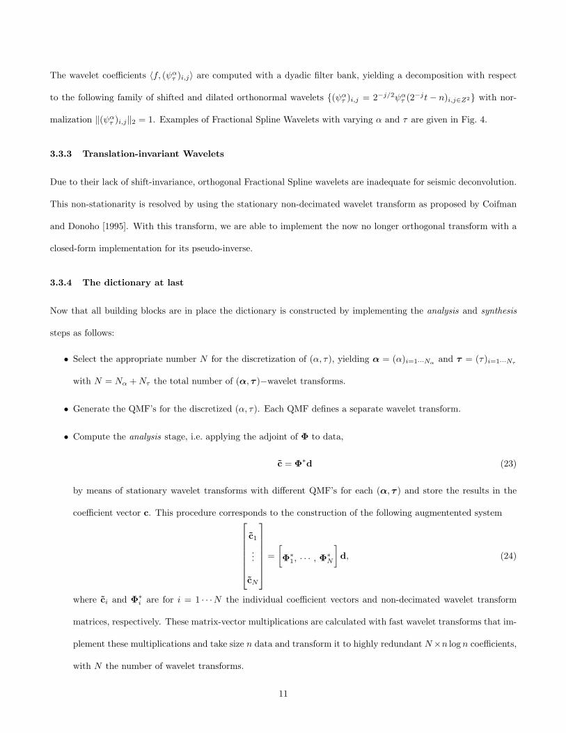
The wavelet coefficients 〈f, (ψατ )i,j〉 are computed with a dyadic filter bank, yielding a decomposition with respect

to the following family of shifted and dilated orthonormal wavelets {(ψατ )i,j = 2−j/2ψα

τ (2−jt− n)i,j∈Z2} with nor-

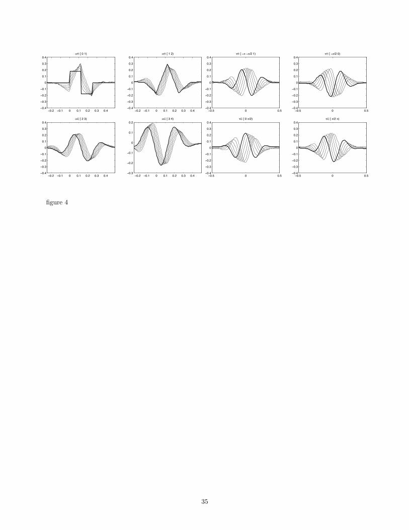
malization ‖(ψατ )i,j‖2 = 1. Examples of Fractional Spline Wavelets with varying α and τ are given in Fig. 4.

3.3.3 Translation-invariant Wavelets

Due to their lack of shift-invariance, orthogonal Fractional Spline wavelets are inadequate for seismic deconvolution.

This non-stationarity is resolved by using the stationary non-decimated wavelet transform as proposed by Coifman

and Donoho [1995]. With this transform, we are able to implement the now no longer orthogonal transform with a

closed-form implementation for its pseudo-inverse.

3.3.4 The dictionary at last

Now that all building blocks are in place the dictionary is constructed by implementing the analysis and synthesis

steps as follows:

• Select the appropriate number N for the discretization of (α, τ), yielding α = (α)i=1···Nαand τ = (τ)i=1···Nτ

with N = Nα +Nτ the total number of (α, τ )−wavelet transforms.

• Generate the QMF’s for the discretized (α, τ). Each QMF defines a separate wavelet transform.

• Compute the analysis stage, i.e. applying the adjoint of Φ to data,

c = Φ∗d (23)

by means of stationary wavelet transforms with different QMF’s for each (α, τ ) and store the results in the

coefficient vector c. This procedure corresponds to the construction of the following augmentented systemc1

...

cN

=[Φ∗

1, · · · , Φ∗N

]d, (24)

where ci and Φ∗i are for i = 1 · · ·N the individual coefficient vectors and non-decimated wavelet transform

matrices, respectively. These matrix-vector multiplications are calculated with fast wavelet transforms that im-

plement these multiplications and take size n data and transform it to highly redundant N×n log n coefficients,

with N the number of wavelet transforms.

11

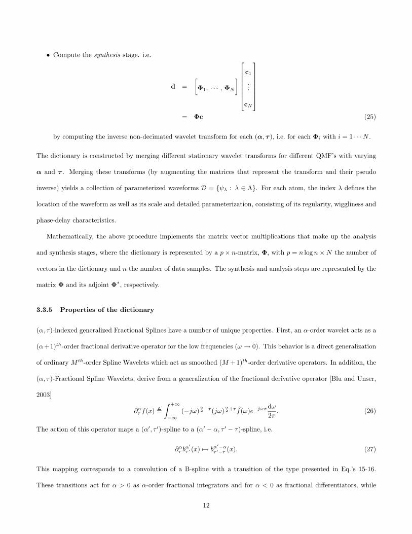
• Compute the synthesis stage. i.e.

d =[Φ1, · · · , ΦN

]

c1

...

cN

= Φc (25)

by computing the inverse non-decimated wavelet transform for each (α, τ ), i.e. for each Φi with i = 1 · · ·N .

The dictionary is constructed by merging different stationary wavelet transforms for different QMF’s with varying

α and τ . Merging these transforms (by augmenting the matrices that represent the transform and their pseudo

inverse) yields a collection of parameterized waveforms D = {ψλ : λ ∈ Λ}. For each atom, the index λ defines the

location of the waveform as well as its scale and detailed parameterization, consisting of its regularity, wiggliness and

phase-delay characteristics.

Mathematically, the above procedure implements the matrix vector multiplications that make up the analysis

and synthesis stages, where the dictionary is represented by a p× n-matrix, Φ, with p = n log n×N the number of

vectors in the dictionary and n the number of data samples. The synthesis and analysis steps are represented by the

matrix Φ and its adjoint Φ∗, respectively.

3.3.5 Properties of the dictionary

(α, τ)-indexed generalized Fractional Splines have a number of unique properties. First, an α-order wavelet acts as a

(α+1)th-order fractional derivative operator for the low frequencies (ω → 0). This behavior is a direct generalization

of ordinary M th-order Spline Wavelets which act as smoothed (M +1)th-order derivative operators. In addition, the

(α, τ)-Fractional Spline Wavelets, derive from a generalization of the fractional derivative operator [Blu and Unser,

2003]

∂ατ f(x) ,

∫ +∞

−∞(−jω)

α2−τ (jω)

α2 +τ f(ω)e−jωx dω

2π. (26)

The action of this operator maps a (α′, τ ′)-spline to a (α′ − α, τ ′ − τ)-spline, i.e.

∂ατ b

α′

τ ′ (x) 7→ bα′−α

τ ′−τ (x). (27)

This mapping corresponds to a convolution of a B-spline with a transition of the type presented in Eq.’s 15-16.

These transitions act for α > 0 as α-order fractional integrators and for α < 0 as fractional differentiators, while

12

they also invoke an additional phase rotation. Consequently, the transition-seismic wavelet interaction corresponds

to an additive property on the parameterization, mapping the waveforms from one family of generalized B-splines to

another.

The above properties for Fractional Splines carry over to (α, τ)-wavelets. The magnitude of these wavelets behave

as

|ψατ (ω)| ∼ |ωα+1| as ω → 0, (28)

corresponding to a (α+ 1)th-order fractional differentiation for the low frequencies. The phase behavior is given by

θ(ω) = tan−1 ={ψατ (ω)}

<{ψατ (ω)}

= 2π · τ. (29)

With this construction of stationary wavelets maximal control over the time-frequency and phase characteristics of

the atoms has been accomplished. Not only is the time-frequency location and spread parameterized but there is

also control over fine-tuning parameters such as the decay, regularity and wiggliness properties as well as the phase

characteristics. Since the definition of seismic reflectivity and the seismic source-function both involve differentiations,

seismic reflection records can be considered as smoothed derivatives, justifying our choice of using Fractional Spline

wavelets. In the next section, two complementary methods are discussed to find a sparse coefficient vector and hence

obtain detailed reflector information.

4 Seismic Atomic Deconvolution

With the successful construction of the versatile Fractional Spline dictionary, we now arrive at our main second

task of solving the seismic deconvolution problem by selecting the appropriate waveforms from the dictionary. The

dictionary is designed to represent reflection events that are given by the convolutional interplay of the parameterized

source-function and reflector-model. The synthesis step corresponding to the forward model is given by the following

matrix-vector multiplication

d = Φc. (30)

The different parameterized waveforms reside in the columns of the Φ-matrix. The coefficient vector c is designed

to be sparse and the question is how to find these sparse entries given (noisy) data. Finding the sparse entries

is an ill-posed problem because the dictionary is redundant leading to an underdetermined system with a highly

13

rectangular matrix Φ. As a result, the analysis stage

c = Φ∗d, (31)

does not give sufficient information to uniquely synthesize data and this leads to

• large differences in sparseness between c and c;

• lack of resolution;

• inferior denoising capabilities;

• a failure to obtain super-resolution, resolving features beyond the resolution admitted by the normal operator

Φ∗Φ.

As in Basis Pursuit [Chen et al., 2001], we will compare three different strategies to obtain the coefficient vector

with emphasis on the seismic application and the selection of a sparse coefficient vector pertaining to the dictionary

detailed in the previous section. Comparisons are made between the Method of Frames (MOF), Matching Pursuit

(MP) and Basis Pursuit (BP). While the first and the last methods are based on solving a global optimization

problem, the second method uses a “local” greedy search algorithm.

To be more specific, the three solution methods correspond in the noise-free situation to solving the following

variational problems [Chen et al., 2001]

c : min ‖c‖p subject to Φc = d (32)

for p = 2, p = 0 and p = 1, respectively. For

• p = 2: the problem corresponds to MOF, which minimizes the coefficients energy by the method of Conjugate

Gradients solving for the system

ΦΦ∗y = d (33)

c† = Φ∗y, (34)

yielding

c† = Φ†d = Φ∗ (ΦΦ∗)−1 d (35)

14

with the matrix Φ† the pseudo-inverse of Φ.

• p = 0: this problem corresponds to MP, which aims to solve a non-convex optimization problem, yielding

non-unique and sensitive solutions. MP minimizes the number of selected atoms by applying a simple recursive

rule that selects the best matching atoms with a “greedy” search strategy.

• p = 1; this problem corresponds to BP, yielding a sparseness-constraint global optimization scheme.

We will now discuss these different strategies to the decomposition and denoising problem, which takes for MOF

(p = 2) and BP (p = 1) the form

minc

:12‖d− Φc‖22 + ν‖c‖p, (36)

with ν a noise-level dependent control parameter. In this study, use is made of an adaptation of Chen’s Atomizer

Software in conjunction with WaveLab, the Rice Wavelet Toolbox and Unser and Blu’s Fractional Spline

refinement filter routines.

4.1 Method of Frames (MOF)

Conjugate Gradients is used to compute the pseudo-inverse of Eq. 35, by jointly minimizing the data-reconstruction

mismatch and the energy of the coefficients for a dictionary consisting of (α, τ)-wavelets. For the noisy case, the

MOF takes the form

(Φ∗Φ + νI) c = Φ∗d, (37)

where the regularization-parameter ν depends on the variance of the noise and the cardinality of the dictionary [Chen

et al., 2001], i.e.

ν = σ√

2 log p (38)

with σ the standard-deviation of the noise.

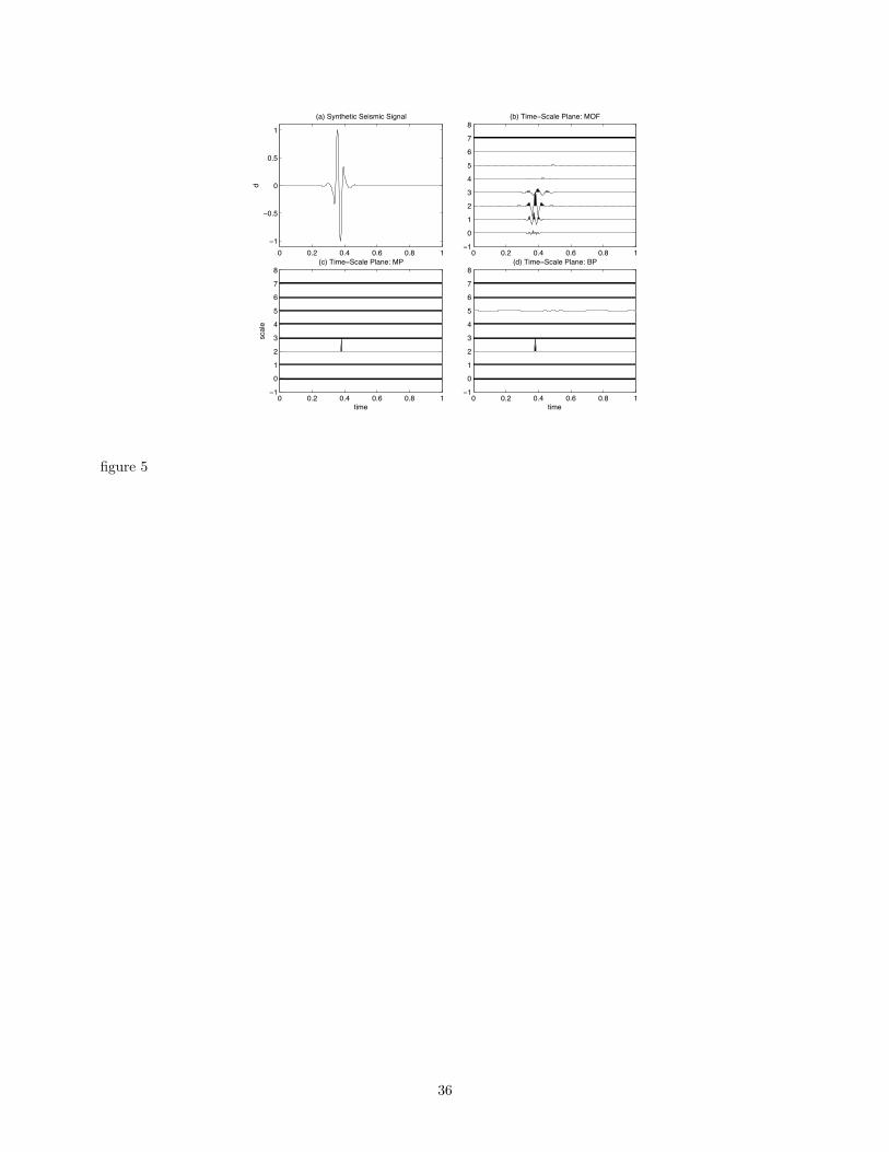
Even though the MOF is a very powerful method with many applications, it fails in highly underdetermined

problems, i.e. large redundancies in the dictionary, to come up with a sparse coefficient vector as can be seen from

Fig. 5. This lack of resolution is due to non-uniqueness diffusing the signal’s energy over many coefficients. This lack

of resolution not only renders MOF ineffective for locating and characterizing reflection events but it also seriously

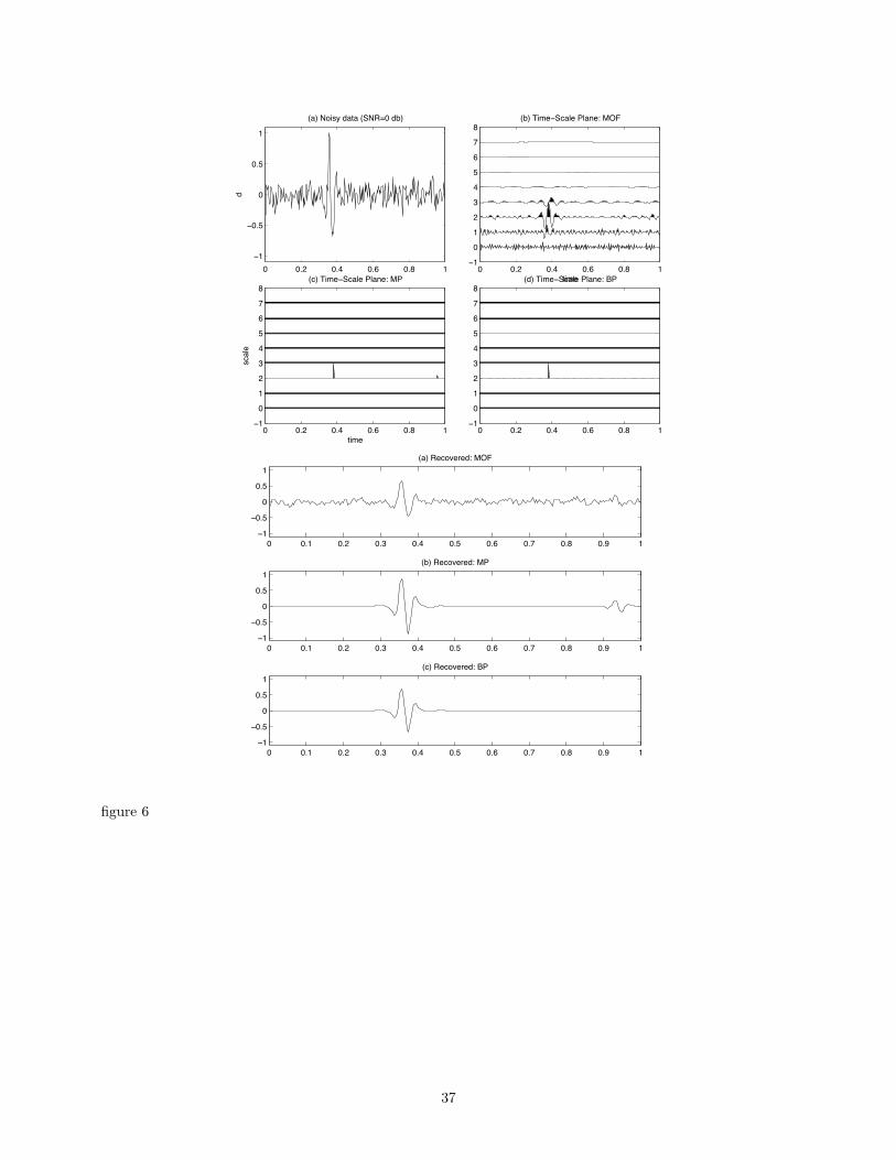
deteriorates the denoising results as can be observed from Fig. 6.

15

In the next two sections, two complementary methods MP and BP will be reviewed that preserve the sparseness

of the decomposition by following two distinct strategies. The first method uses a bottom-up approach, which starts

with a very sparse decomposition to which successively more detail is added to improve the approximation. The

second method follows an opposite strategy. BP starts with the “full” decomposition, which is subsequently sparsified

by imposing the L1-norm on the coefficients.

4.2 Solution by Matching Pursuit (MP)

Greedy search algorithms such as Matching Pursuit [Mallat, 1997] approximate data d for each iteration by selecting

atoms from the dictionary D that minimize the L2-difference between subsequent reductions and remaining atoms

in the dictionary. Reductions are projections of d

d = 〈d,gλ0〉gλ0

+Rd, (39)

where Rd is the residue and gλ0the particular λ0-indexed atom that maximizes the correlation [Mallat, 1997], i.e.

|〈Rd,gλ0〉| ≥ sup

λ∈Λ|〈Rd,gλ〉|. (40)

The index λ ∈ Λ labels the atom and determines the atom’s parameterization. By initializing R0d = d and repeating

the above reductions with the following update rule for the mth iteration

Rmd = 〈Rmd,gλm〉gλm

+Rm+1d, (41)

we obtain by computing the following inner products

〈Rmd,gλ〉 = 〈Rmd,gλm〉gλm

+ 〈Rm+1d,gλm〉〈gλm

,gλ〉 (42)

an iterative scheme that computes a sparse approximation for d,

d =M∑

m=1

〈d,gλm〉gλm

(43)

= Φc. (44)

As M → ∞, this decomposition not only becomes exact, it also provides a sparse approximate representation if we

let M �∞. The adaptivity of the dictionary and the subsequent selection of the best fitting atoms concentrate the

data’s energy in as few as possible number of atoms, yielding a high non-linear approximation rate.

16

Because of the high non-linear approximation rate, the adaptive MP decomposition provides an effective denoising

scheme by only selecting the coherent events. Coherent events are atoms for which

|〈RMd,gλM〉|

‖RMd‖> noise level. (45)

MP forms the basis of earlier work [Herrmann, 2003a,b, Herrmann and de Hoop, 2002], where MP was applied to

denoise and characterize seismic images with moderate to good success. As we can see from Fig. 1, there are problems

with this decomposition method, which may give rise to sudden sign-changes, non-unique decompositions and lack

of lateral continuity. While the first two problems are likely related to certain shortcomings of the dictionary, which

is fundamentally one-dimensional and lacks sufficiently precise phase-delay characterization, the non-uniqueness is a

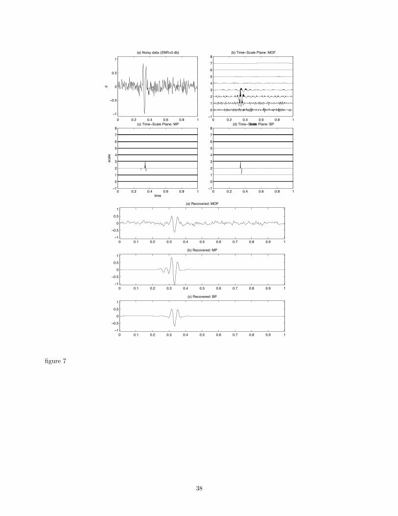
more serious problem as can be inferred from Fig. 7. In that figure, MP fails to recover two closely spaced atoms

(even for the noise-free case). This failure is due the greediness of the algorithm, which may lead MP to wander off

in the wrong direction leading the selection of many atoms. Even though these selected atoms may reconstruct the

signal explaining the successful denoising, they do not carry information on the types of waveforms hidden in the

seismic record. As shown below BP, may overcome this problem and is able to resolve the two waveforms.

4.3 Solution by Basis Pursuit (BP)

As an alternative to the greedy algorithm MP, BP solves for the sparse decomposition by replacing the global

quadratic penalty term in MOF by a non-quadratic global L1-norm. Imposing this L1-norm enforces sparseness on

the initially full coefficient vector. Sparseness constraints are not new to seismic processing and inversion [Levy et al.,

1988, Oldenburg et al., 1981, 1988, Sacchi et al., 1994, Scheuer, 81, Schonewille and Duijndam, 2001, Ulrych and

Walker, 1982]), but the major difference in this approach is that sparseness is imposed on coefficients rather than

directly on the reflectivity itself. In this way, we explore fully the adaptivity of the dictionary and hope to be less

sensitive to apparent bandwidth limitation.

In the noise-free case, BP-decomposition takes the form

c : min ‖c‖1 subject to Φc = s, (46)

where the L1-norm on the coefficients is minimized subject to a reconstruction of the signal d by superposition over

the waveforms (elements in the dictionary D).

17

For noisy data BP-denoising solves

c : minc

12‖d− Φc‖22 + ν‖c‖1, (47)

which corresponds to the joint minimization of the L2-difference between noise data and the weighted L1-norm on

the coefficients. The rationale behind the particular choice for the control parameter (cf. Eq. 38)

νp = σ√

2 log p (48)

lies in the fact that for orthonormal decompositions SureShrink soft-thresholding of noisy coefficients [Chen et al.,

2001, Donoho and Johnstone, 1998, Lucier, 2001, Mallat, 1997] solves the minimization problem of Eq. 47. For our

dictionary, the cardinality equals p = n log n × N . For the actual solution of Eq. 46 and 47, we resort to methods

developed in Linear Programming [Gill, 1991]. We use the same pdsco-optimizer as used in the Atomizer Toolbox

to solve the standard form

minx

w∗x subject to Ax = b, x ≥ 0, (49)

which was obtained by the following reformulation of Eq. 46 [Chen et al., 2001, Coifman and Donoho, 1995, Mallat,

1997]

A =(Φ −Φ

), x =

u

v

, b = d, w = ν

1

1

. (50)

In this formulation u ≥ 0 and v ≥ 0 are two “slack variables” such that c = u− v yielding ‖c‖1 = ‖u‖1 + ‖v‖1. For

noise-free decompositions (σ = 0), we set ν = 1 and solve Eq. 50. For noisy data we set ν = σ√

2 log p and solve the

perturbed linear program:

minx,p

w∗x subject to Ax + δp = b, x ≥ 0, δ = 1. (51)

A solution of this program is obtained by using a Primal-Dual Log-Barrier LP Algorithm based on Saunder’s pdco-

routine. This scheme solves the equivalent perturbed dual linear program [Chen et al., 2001] and involves regulariza-

tion parameters that are set according to whether one is decomposing; trying to obtain super-resolution or dealing

with noisy data. The algorithm starts with an initial feasible solution yielded by MOF and then proceeds by applying

the Log-barrier algorithm. The speed of the algorithm depends on the data’s complexity; the size of the dictionary,

the number of barrier iterations and the accuracy of the Conjugate Gradient Solver (LSQR [Paige and Saunders,

1982]). Both synthetic and real data examples are discussed below.

18

5 Application to seismic data

To study the properties of the developed dictionary and the associated decomposition strategies, a number of ad-

ditional tests are conducted on synthetic and real datasets. These tests are designed to pinpoint the merits and

possible shortcomings of the different methods.

5.1 Comparative study on synthetic seismic traces

The synthetic examples included so far in Fig.’s 2-7 dealt with relatively small dictionaries and moderate complexity

for the reflection data. We will now show examples where we gradually increase the complexity of the seismic records

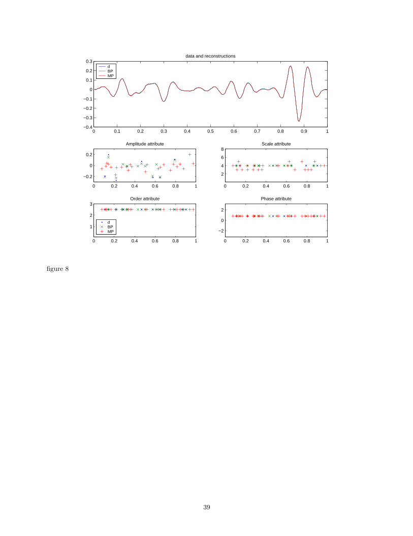
and the size of the dictionary. Fig. 8 shows the decomposition of a signal consisting of 10 atoms that are randomly

(according to a cumulative Poisson process) positioned with log-normal distributed amplitudes. The dictionary in

this example consists of a single (α, τ)-pair non-decimated wavelet transform with α = 2.5 and τ = 1/4π. The

coefficients were selected to yield a constant scale. The signal is perfectly reconstructed both for MP and BP.

However, close inspection of the selected atoms shows that there are major differences between the estimates yielded

by these two methods. Despite some minor amplitude differences between the original and estimated coefficients,

BP is able to accurately recover the location of the coefficients and is able to estimate the atom’s parameterization

from the signal. MP on the other hand, selects atoms with erroneous scales and introduces spurious events that are

not linked to atoms that were originally used to generate the seismic trace. Increasing the complexity by increasing

the number of events in the seismic trace makes the situation worse and eventually leads to a breakdown of BP as

well.

For larger dictionaries, we were only able to recover the atoms with their attributes by using MP for seismic

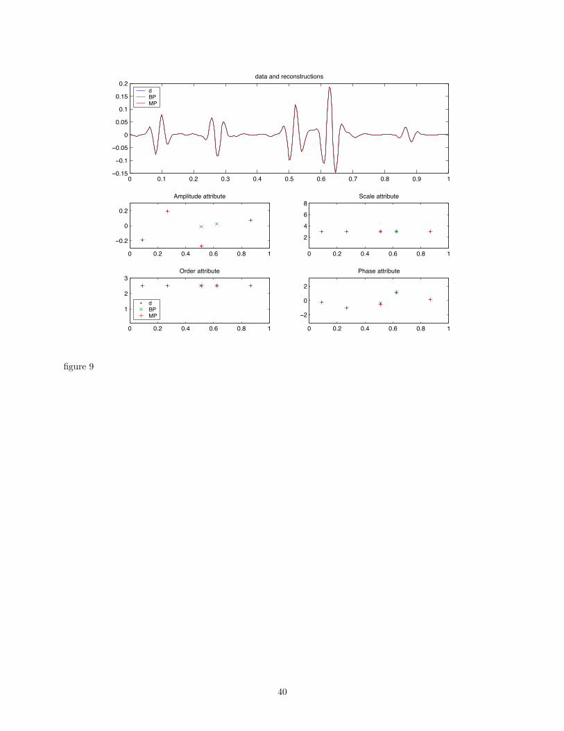
records with an increased frequency content and decreased number of events. Fig. 9 displays the results for a

dictionary consisting of wavelet transforms for fixed α = 2.5 and 25 different phase-delays with τ ∈ [−π, π]. With

its greedy strategy, MP is able to recover the waveforms, an observation that also applies to a dictionary generated

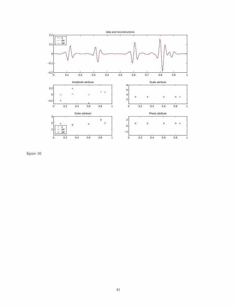
for a fixed τ = 1/4π phase-delay and 25 varying order α ∈ [1.5, 2.5] wavelets. See Fig. 10 for detail. The results for

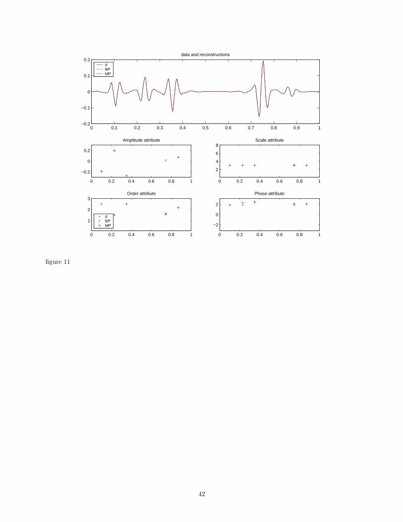
a dictionary consisting of 100 wavelet transforms are summarized in Fig. 11. In this example, both the phase-delay

and order are allowed to vary, α ∈ [1.5, 2.5] and τ ∈ [−π, π]. Again MP is able to select atoms that are close to the

original ones. So what do these three examples have in common such that MP works while BP fails?

19

Compared to the dictionaries consisting for example of sinusoids and deltas [Chen et al., 2001], our dictionary

contains waveforms that resemble each other quite closely. As a consequence, the projection of our dictionary onto

the events in the signal yields inner products that only differ slightly. For sufficiently simple configurations, these

differences are sufficient for MP to select the correct waveforms. BP, on the other hand, suffers from the fact that

the L1-norm has a tendency to equally distribute the energy amongst atoms with similar correlations, yielding small

variations in the inner products. So for a large dictionary, there too many of these atoms and consequently BP fails

for configurations that consist of several events. However, the example in Fig. 7 shows that for simple configurations

and not too large dictionaries BP is able to recover the waveforms and hence solve the deconvolution problem with

super-resolution.

5.2 Application to a seismic shot record

Despite the above difficulties to obtain decompositions that lend themselves for a determination of the reflector

attributes, both BP and MP are able to locate seismic events when the dictionary consists of a single wavelet

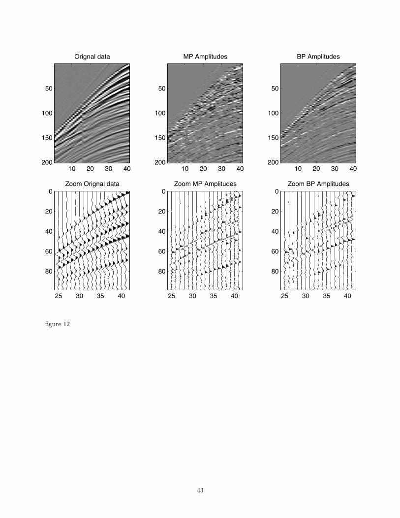
transform. In Fig. 12, the results of these decompositions are summarized for a wavelet with α = 2.5 and τ = π/4.

It is difficult to make definite inferences from the decomposition results presented in this figure. BP shows a better

lateral continuity for the reflectors especially in the region of large complexity (top right). The amplitudes themselves

are inconclusive and difficult to interpret.

5.3 Seismic interpretation and application to seismic imaging

To characterize the major singularities within a real data seismic image we submit the results of the denoising

example in Fig. 1(left) taken from Herrmann [2003a] to the Matching Pursuit Decomposition algorithm. This data

contains an image of the Valhall which contains a very complicated broken chalk reservoir.

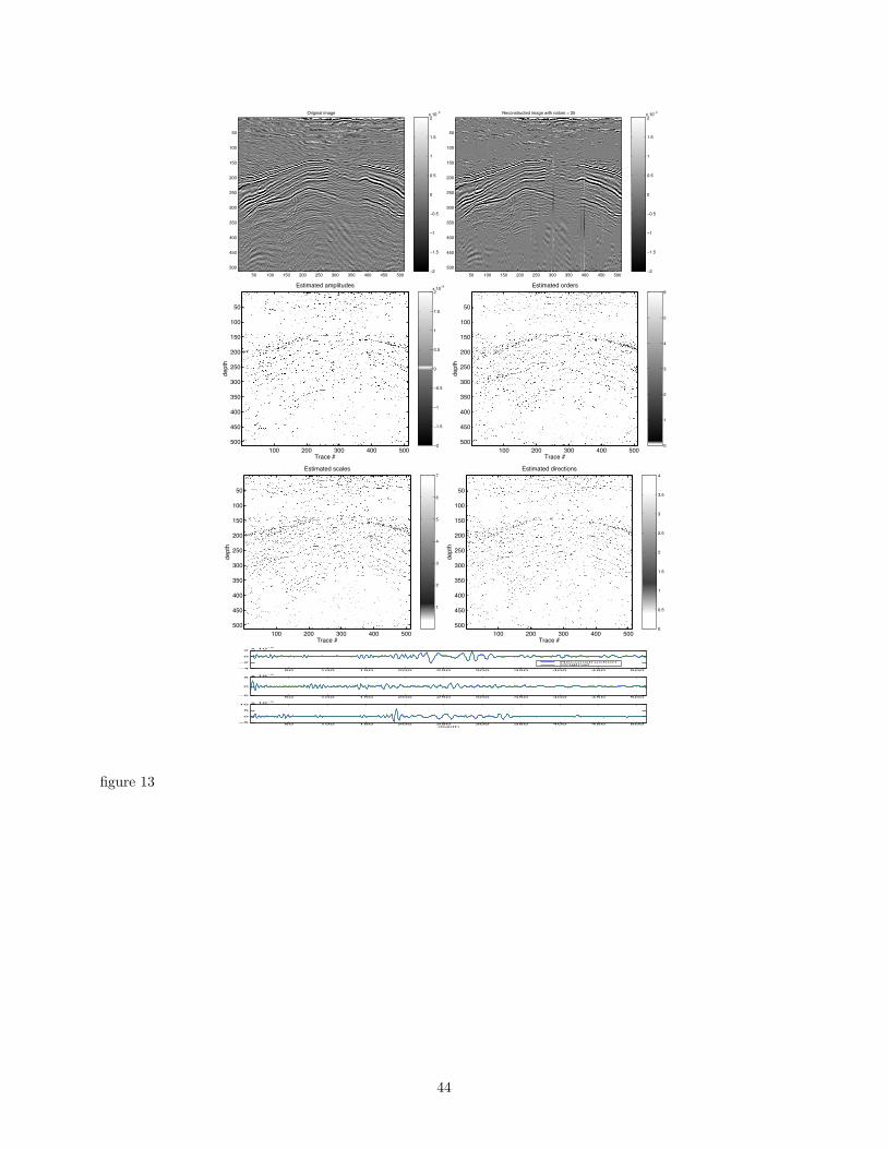
We ran the algorithm for each trace (each lateral position) and we took 50 different values for α of the Fractional

Spline Wavelets ranging α ∈ [0.5 5] and τ = 0. We allowed for 25 estimated atoms per trace. Results of this

decomposition are shown in Fig. 13 from which we can make the following observations:

• major singularities in the image are reconstructed (compare top row in Fig. 13) by only the first 25 atoms using

Eq.43, which corresponds to a compression ratio of 0.0488. There are some slight artifacts where very coarse

20

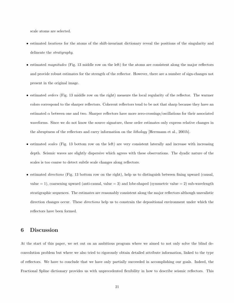
scale atoms are selected.

• estimated locations for the atoms of the shift-invariant dictionary reveal the positions of the singularity and

delineate the stratigraphy.

• estimated magnitudes (Fig. 13 middle row on the left) for the atoms are consistent along the major reflectors

and provide robust estimates for the strength of the reflector. However, there are a number of sign-changes not

present in the original image.

• estimated orders (Fig. 13 middle row on the right) measure the local regularity of the reflector. The warmer

colors correspond to the sharper reflectors. Coherent reflectors tend to be not that sharp because they have an

estimated α between one and two. Sharper reflectors have more zero-crossings/oscillations for their associated

waveforms. Since we do not know the source signature, these order estimates only express relative changes in

the abruptness of the reflectors and carry information on the lithology [Herrmann et al., 2001b].

• estimated scales (Fig. 13 bottom row on the left) are very consistent laterally and increase with increasing

depth. Seismic waves are slightly dispersive which agrees with these observations. The dyadic nature of the

scales is too coarse to detect subtle scale changes along reflectors.

• estimated directions (Fig. 13 bottom row on the right), help us to distinguish between fining upward (causal,

value = 1), coarsening upward (anti-causal, value = 3) and lobe-shaped (symmetric value = 2) sub-wavelength

stratigraphic sequences. The estimates are reasonably consistent along the major reflectors although unrealistic

direction changes occur. These directions help us to constrain the depositional environment under which the

reflectors have been formed.

6 Discussion

At the start of this paper, we set out on an ambitious program where we aimed to not only solve the blind de-

convolution problem but where we also tried to rigorously obtain detailed attribute information, linked to the type

of reflectors. We have to conclude that we have only partially succeeded in accomplishing our goals. Indeed, the

Fractional Spline dictionary provides us with unprecedented flexibility in how to describe seismic reflectors. This

21

generalization is highly useful because this representation naturally captures the reflector’s sharpness and instanta-

neous phase characteristics both of which are of direct relevance to the underlying lithology and rock-physics. The

Fractional Spline framework also yielded fast numerical implementation of non-decimated wavelets by means of filter

banks making the decomposition numerically feasible. As such, the construction led to shift-invariant waveforms

that for the low frequencies behave as fractional derivative operators designed to match the local aspects of reflec-

tion events, which can also be regarded as smoothed derivative operators. Hence, our choice for Fractional Spline

Wavelets. Since sedimentary records show evidence of multi-fractal behavior the local adaption to singularity-order

by means of the order of the Fractional Spline seems to have been a natural choice with potential.

The scaling complexity of sedimentary basins as translated in the seismic records certainly justifies the construc-

tion of the Fractional Spline dictionary. However, on the same token the flexibility of the dictionary, where each

non-decimated wavelet transform forms a complete basis, makes the problem of finding the appropriate atoms from

the dictionary that much harder. In fact, the decomposition is a NP-hard problem and this perhaps explains our

difficulties finding the correct decomposition for very redundant dictionaries with waveforms that only differ in the

details of their regularity and phase characteristics.

Even though, it proved to be difficult to assign definite interpretations to the selected atoms, we obtained the

following results. (i) The proposed dictionary captures details on the sharpness and phase characteristics of the

reflectors and constitutes a departure from reflector models, based on either statistical homogeneity arguments or

on a piece-wise continuous Earth model, yielding spike trains for the reflectivity. (ii) For simple configurations and

modest size dictionaries, BP was able to obtain super-resolution, unraveling two closely spaced waveforms. This

makes BP the pre-eminent choice for decomposing the local complexity along a single major unconformity. MP

in these cases yields erroneous results because of “interference” between atoms, an observation consistent with the

literature. (iii) For more extensive dictionaries, BP fails because the L1-norm has the tendency to equally distribute

the signal’s energy amongst waveforms that closely match reflection events. MP succeeds in cases where the individual

events are sufficiently isolated so that “interference” can be neglected. (iv) For dictionaries consisting of a single

wavelet transform, both BP and MP obtain reasonable results delineating the stratigraphy and hence solving part of

the deconvolution problem. BP appears to obtain a better lateral continuity especially in a region of large complexity.

(v) Mathematically, our decomposition corresponds to finding Multi-fractional Spline Representation where the

22

atom’s parameterization contains information on (1) the location of the nodes of the Fractional Splines; (2) relative

magnitude of the reflectors; (3) relative changes (modulo the source-function) in the local regularity of the reflector

parameterized by the order α; (4) relative changes (modulo the source-function) in instantaneous phase τ and (5) the

dominant frequency (the scale) which is a function of the seismic wavelet, possible dispersion, imaging blurring and

a characteristic scale of the reflector. (vi) Finally, application of MP to an imaged seismic dataset showed that our

non-linear decomposition method and dictionary provide useful information. However, higher dimensional extensions

will be necessary to improve the lateral continuity.

The bottleneck in the non-linear approaches presented in this paper is that the methods either suffer from

sensitivities, when the waveforms “interfere” yielding waveforms that are not present in the dictionary, or from the

inability of the L1-norm to impose sparseness for a highly redundant dictionary with waveforms that are relative

close in their behavior. In that sense, our problem turns out to be similar to many (geophysical) inversion problems

plagued by non-uniqueness. However, we hope to report in a future paper on an approach where we use information

on the multifractial singularity spectrum to remove some of the non-uniqueness associated with the blind seismic

deconvolution for a highly intermittent reflectivity.

Since the initial submission of this paper, the author has become aware of recent work on decompositions with

respect to highly redundant dictionaries [Starck et al., 2004]. Above qualitative observations with regard to MP’s and

BP’s inability to uniquely decompose the signal with respect to dictionaries defined by multiple wavelet transforms

can be made quantitative through the introduction of the spark and mutual incoherence of a dictionary. This spark

measures the redundancy of the dictionary and provides sparseness conditions on the estimated coefficient vector

which guarantee uniqueness. In a future paper, we will report on how to use the spark measure in conjunction with

block solvers to uniquely solve the parameterized blind deconvolution problem as posed in this paper.

Acknowledgements

We like to thank the Valhall license partners BP, Shell, Total and Amerada Hess for permission to publish their data;

the makers of Wavelab, Atomizer and Rice Wavelet Toolbox, Michael Unser and Thierry Blu for making

their software available. This work was financially supported by a NSERC Discovery Grant and by a Grant in Aid

by ChevronTexaco as part of the ChaRM Project.

23

References

T. Blu and M. Unser. A complete family of scaling functions: The (α, τ)-fractional splines. In Proceed-

ings of the Twenty-Eighth International Conference on Acoustics, Speech, and Signal Processing (ICASSP’03),

volume VI, pages 421–424, Hong Kong SAR, People’s Republic of China, April 6-10, 2003. URL

http://bigwww.epfl.ch/publications/blu0301.html.

Thierry Blu and Michael Unser. The fractional spline wavelet transform: Definition and implementation. In Pro-

ceedings, volume I, pages 512–515. IEEE, 2000.

S. Brandsberg-Dahl and M. de Hoop. Focusing in dip and ava compensation on scattering-angle/azimuth common

image gathers. Geophysics, 68(1):232–254, 2003.

Scott Shaobing Chen, David L. Donoho, and Michael A. Saunders. Atomic decomposition by basis pursuit. SIAM

Journal on Scientific Computing, 43(1):129–159, 2001.

R. R. Coifman and D. L. Donoho. Translation-invariant de-noising. Technical report, Stanford, Department of

Statistics, 1995. URL citeseer.nj.nec.com/80329.html.

F. J. Dessing. A wavelet transform approach to seismic processing. PhD thesis, Delft University of Technology, Delft,

the Netherlands, 1997.

David L. Donoho and Iain M. Johnstone. Minimax estimation via wavelet shrinkage. Annals of Statistics, 26(3):

879–921, 1998. URL citeseer.nj.nec.com/donoho92minimax.html.

P. Gill. Numerical Linear Algebra and Optimization. Addison Wesley, 1991.

J. Harms and P. Tackenberg. Seismic signatures of sedimentation models. Geophysics, 37(1):45–58, 1972.

Felix J. Herrmann. Multiscale analysis of well and seismic data. In Siamak Hassanzadeh, editor,

Mathematical Methods in Geophysical Imaging V, volume 3453, pages 180–208. SPIE, 1998. URL

http://www.eos.ubc.ca/ felix/Preprint/SPIE.ps.gz.

Felix J. Herrmann. Fractional spline matching pursuit: a quantitative tool for seismic stratigraphy. In Expanded

Abstracts, Tulsa, 2001a. Soc. Expl. Geophys. URL http://www.eos.ubc.ca/ felix/Preprint/SEG01.ps.gz.

24

Felix J. Herrmann. Singularity characterization by monoscale analysis. Appl. Comput. Harmon. Anal., 11(4):64–88,

July 2001b.

Felix J. Herrmann. Multifractional splines: application to seismic imaging. In Andrew F. Laine; Eds.

Michael A. Unser, Akram Aldroubi, editor, Proceedings of SPIE Technical Conference on Wavelets:

Applications in Signal and Image Processing X, volume 5207, pages 240–258. SPIE, 2003a. URL

http://www.eos.ubc.ca/ felix/Preprint/SPIE03DEF.pdf.

Felix J. Herrmann. Optimal seismic imaging with curvelets. In Expanded Abstracts, Tulsa, 2003b. Soc. Expl. Geophys.

URL http://www.eos.ubc.ca/ felix/Preprint/SEG03.pdf.

Felix J. Herrmann and Yves Bernabe. Seismic singularities at upper mantle discontinuities: a site percolation model.

2004. accepted for publication.

Felix J. Herrmann and Martijn de Hoop. Edge preserved denoising and singularity extrac-

tion from angles gathers. In Expanded Abstracts, Tulsa, 2002. Soc. Expl. Geophys. URL

http://www.eos.ubc.ca/ felix/Preprint/SEG02.pdf.

Felix J. Herrmann, William Lyons, and Colin Stark. Seismic facies characterization by monoscale analysis. Geoph.

Res. Lett., 28(19):3781–3784, 2001a.

Felix J. Herrmann, William Lyons, and Colin Stark. Seismic facies characterization by monoscale analysis. Geoph.

Res. Lett., 28(19):3781–3784, Oct. 2001b. URL http://www.eos.ubc.ca/ felix/Preprint/WellSeis.ps.gz.

F.J. Herrmann. A scaling medium representation, a discussion on well-logs, fractals and

waves. PhD thesis, Delft University of Technology, Delft, the Netherlands, 1997. URL

http://www.eos.ubc.ca/ felix/Preprint/PhDthesis.pdf.

J. Hu, G. T. Schuster, and P.A. Valasek. Poststack migration deconvolution. Geophysics, 66(3):939–952, 2001.

H. Kuhl and M. D. Sacchi. Least-squares wave-equation migration for avp/ava inversion. Geophysics, 68(1):262–273,

2003.

S. Levy, D. Oldenburg, and J. Wang. Subsurface imaging using magnetotelluric data. Geophysics, 53(01):104–117,

1988.

25

Bradley J. Lucier. Interpreting translation-invariant wavelet shrinkage as a new image smoothing scale space. IEEE

Transactions on Image Processing, 10:993–1000, 2001.

S. G. Mallat. A wavelet tour of signal processing. Academic Press, 1997.

J. Muller, I. Bokn, and J. L. McCauley. Multifractal analysis of petrophysical data. Ann. Geophysicae, 10:735–761,

1992.

D. W. Oldenburg, S. Levy, and K. P. Whittall. Wavelet estimation and deconvolution. Geophysics, 46(11):1528–1542,

1981.

D. W. Oldenburg, T. Scheuer, and S. Levy. Recovery of the acoustic impedance from reflection seismograms. Inversion

of geophysical data, pages 245–264, 1988.

C. C. Paige and M. A. Saunders. Lsqr: An algorithm for sparse linear equations and sparse least squares. ACM

TOMS, 8(1):43–71, 1982.

Charles Payton, editor. Seismic stratigraphy – applications to hydrocarbon exploration, chapter Stratigraphic models

from seismic data. AAPG, 1977.

E. A. Robinson. Predictive decomposition of seismic traces. Geophysics, 22(04):767–778, 1957.

M. D. Sacchi, D. R. Velis, and A. H. Cominguez. Minimum entropy deconvolution with frequency-domain constraints.

Geophysics, 59(06):938–945, 1994.

M.M. Saggaf and E. A. Robinson. A unified framework for the deconvolution of traces of nonwhite reflectivity.

Geophysics, 65(5):1660–1676, 2000.

A. Saucier and J. Muller. Use of multifractal analysis in the characterization of geological formation. Fractals, 1(3):

617–628, 1993.

T. Scheuer. The recovery of subsurface reflectivity and impedance structure from reflection seismograms. Master’s

thesis, Univ. British Columbia, 81.

M.A. Schonewille and A.J.W. Duijndam. Parabolic radon transform, sampling and efficiency. volume 66, pages

667–678. Soc. of Expl. Geophys., 2001.

26

J. L. Starck, M. Elad, and D. Donoho. Redundant multiscale transforms and their application to morphological

component separation. Advances in Imaging and Electron Physics, 132, 2004.

T. P. H. Steeghs. Local Power Spectra and Seismic Interpretation. PhD thesis, Delft University of Technology, 1997.

A.P.E. ten Kroode, D.-J Smit, and A.R. Verdel. A microlocal analysis of migration. Wave Motion, 28, 1998.

Daniel Trad. Implementations and Aapplications of the sparse Radon transform. PhD thesis, University of British

Columbia, 2001.

T. J. Ulrych and C. Walker. Analytic minimum entropy deconvolution. Geophysics, 47(09):1295–1302, 1982.

Michael Unser and Thierry Blu. Fractional splines and wavelets. SIAM Review, 42(1):43–67, 2000.

Frederic Verhelst. Integration of seismic data with well-log data. PhD thesis, Delft University of Technology, 2000.

Curtis Vogel. Computational Methods for Inverse Problems. SIAM, 2002.

C. P. A. Wapenaar. Amplitude-variation-with-angle behavior of self-similar interfaces. Geophysics, 64:1928, 1999.

27

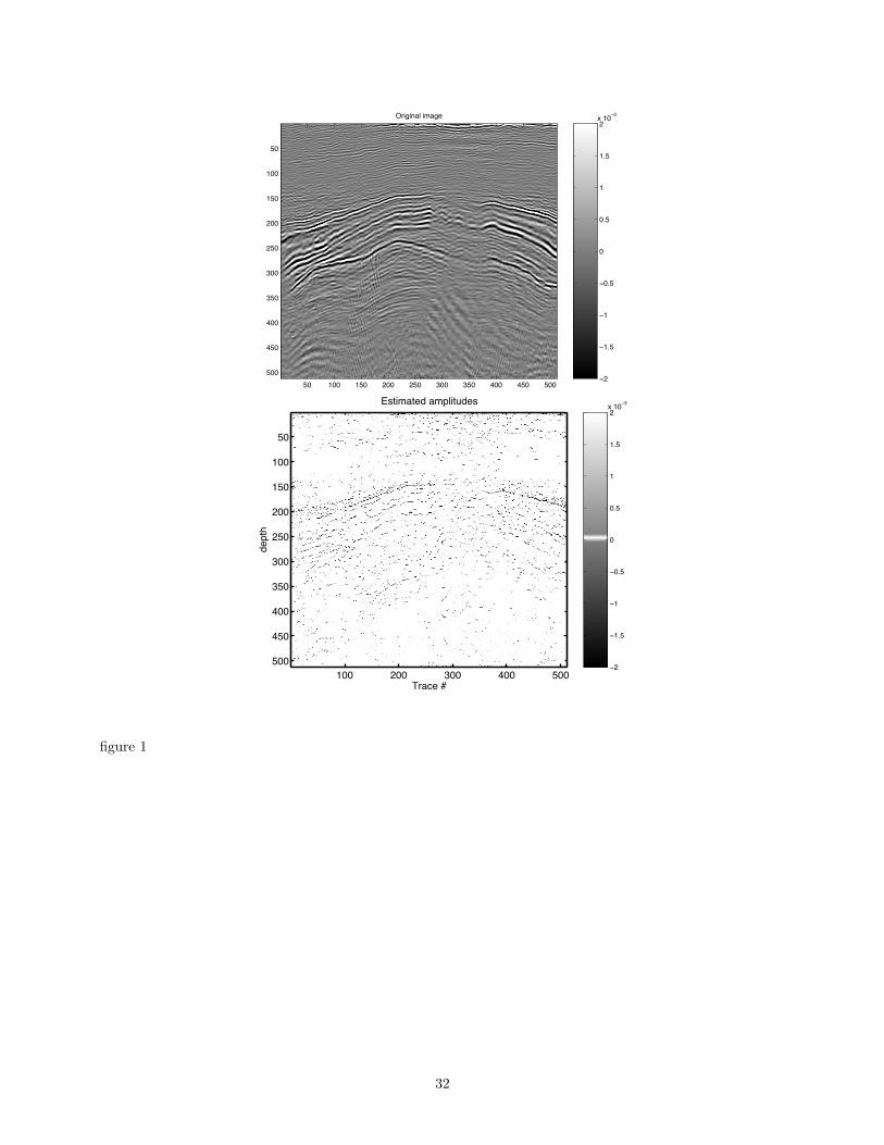
Figure 1: Example of deconvolution and characterization based on Atomic Decomposition (See also Fig. 13). In this

example we applied the greedy MP to denoised (by Curvelet/Contourlet denoising) window of a seismic image taken

from Herrmann [2003a]. The data contains an image of the reservoir of the Valhall. Left: Stacked denoised image.

Right: estimated amplitudes using a decomposition of 25 atoms from the Fractional Spline Wavelet dictionary

introduced in this paper. The stratigraphy is reasonably well recovered from the selected atoms and the estimated

amplitudes can be interpreted as a “spiky” deconvolution.

Figure 2: Example of varying order transitions (left) and their seismic reflectivity for Ricker/Mexican hat wavelet

(second derivative of the Gaussian). The transition orders are set to continuously interpolate between the zero-order

jump-discontinuity (α = 0) and the first-order ramp-function (α = 1). As one can clearly see the reflectivity not

only differs significantly in amplitude but also in waveform. For example, the reflected waveform for α = 0 clearly

resembles the Ricker wavelet while for α = 1 a waveform is observed that resembles the integration of the Ricker

wavelet.

Figure 3: Examples of different transitions and their induced reflected waveforms. First column: the classical zero-

order discontinuity and the Ricker-wavelet reflectivity; Middle column: causal fractional-order transition with its

asymmetric response; Right column: anti-causal fractional-order transition with its response. The causal and

ant-causal transitions are members of a much larger family of splines given by Eq. 18. See Fig 4 for examples of

generalized Fractional Spline wavelets that can be associated with waveforms generated by transitions of the type

given by Eq. 18.

28

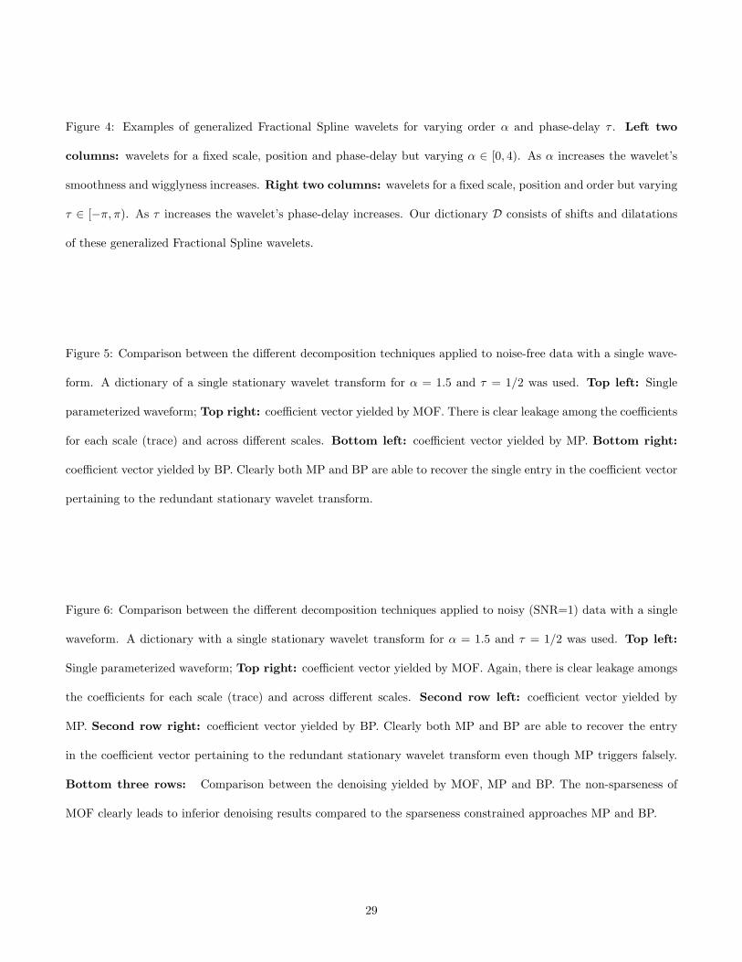
Figure 4: Examples of generalized Fractional Spline wavelets for varying order α and phase-delay τ . Left two

columns: wavelets for a fixed scale, position and phase-delay but varying α ∈ [0, 4). As α increases the wavelet’s

smoothness and wigglyness increases. Right two columns: wavelets for a fixed scale, position and order but varying

τ ∈ [−π, π). As τ increases the wavelet’s phase-delay increases. Our dictionary D consists of shifts and dilatations

of these generalized Fractional Spline wavelets.

Figure 5: Comparison between the different decomposition techniques applied to noise-free data with a single wave-

form. A dictionary of a single stationary wavelet transform for α = 1.5 and τ = 1/2 was used. Top left: Single

parameterized waveform; Top right: coefficient vector yielded by MOF. There is clear leakage among the coefficients

for each scale (trace) and across different scales. Bottom left: coefficient vector yielded by MP. Bottom right:

coefficient vector yielded by BP. Clearly both MP and BP are able to recover the single entry in the coefficient vector

pertaining to the redundant stationary wavelet transform.

Figure 6: Comparison between the different decomposition techniques applied to noisy (SNR=1) data with a single

waveform. A dictionary with a single stationary wavelet transform for α = 1.5 and τ = 1/2 was used. Top left:

Single parameterized waveform; Top right: coefficient vector yielded by MOF. Again, there is clear leakage amongs

the coefficients for each scale (trace) and across different scales. Second row left: coefficient vector yielded by

MP. Second row right: coefficient vector yielded by BP. Clearly both MP and BP are able to recover the entry

in the coefficient vector pertaining to the redundant stationary wavelet transform even though MP triggers falsely.

Bottom three rows: Comparison between the denoising yielded by MOF, MP and BP. The non-sparseness of

MOF clearly leads to inferior denoising results compared to the sparseness constrained approaches MP and BP.

29

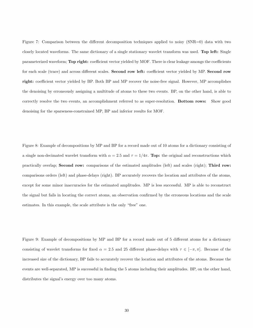
Figure 7: Comparison between the different decomposition techniques applied to noisy (SNR=0) data with two

closely located waveforms. The same dictionary of a single stationary wavelet transform was used. Top left: Single

parameterized waveform; Top right: coefficient vector yielded by MOF. There is clear leakage amongs the coefficients

for each scale (trace) and across different scales. Second row left: coefficient vector yielded by MP. Second row

right: coefficient vector yielded by BP. Both BP and MP recover the noise-free signal. However, MP accomplishes

the denoising by erroneously assigning a multitude of atoms to these two events. BP, on the other hand, is able to

correctly resolve the two events, an accomplishment referred to as super-resolution. Bottom rows: Show good

denoising for the sparseness-constrained MP, BP and inferior results for MOF.

Figure 8: Example of decompositions by MP and BP for a record made out of 10 atoms for a dictionary consisting of

a single non-decimated wavelet transform with α = 2.5 and τ = 1/4π. Top: the original and reconstructions which

practically overlap; Second row: comparisons of the estimated amplitudes (left) and scales (right); Third row:

comparisons orders (left) and phase-delays (right). BP accurately recovers the location and attributes of the atoms,

except for some minor inaccuracies for the estimated amplitudes. MP is less successful. MP is able to reconstruct

the signal but fails in locating the correct atoms, an observation confirmed by the erroneous locations and the scale

estimates. In this example, the scale attribute is the only “free” one.

Figure 9: Example of decompositions by MP and BP for a record made out of 5 different atoms for a dictionary

consisting of wavelet transforms for fixed α = 2.5 and 25 different phase-delays with τ ∈ [−π, π]. Because of the

increased size of the dictionary, BP fails to accurately recover the location and attributes of the atoms. Because the

events are well-separated, MP is successful in finding the 5 atoms including their amplitudes. BP, on the other hand,

distributes the signal’s energy over too many atoms.

30

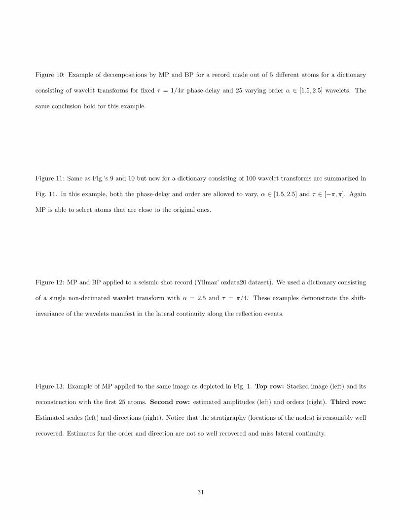
Figure 10: Example of decompositions by MP and BP for a record made out of 5 different atoms for a dictionary

consisting of wavelet transforms for fixed τ = 1/4π phase-delay and 25 varying order α ∈ [1.5, 2.5] wavelets. The

same conclusion hold for this example.

Figure 11: Same as Fig.’s 9 and 10 but now for a dictionary consisting of 100 wavelet transforms are summarized in

Fig. 11. In this example, both the phase-delay and order are allowed to vary, α ∈ [1.5, 2.5] and τ ∈ [−π, π]. Again

MP is able to select atoms that are close to the original ones.

Figure 12: MP and BP applied to a seismic shot record (Yilmaz’ ozdata20 dataset). We used a dictionary consisting

of a single non-decimated wavelet transform with α = 2.5 and τ = π/4. These examples demonstrate the shift-

invariance of the wavelets manifest in the lateral continuity along the reflection events.

Figure 13: Example of MP applied to the same image as depicted in Fig. 1. Top row: Stacked image (left) and its

reconstruction with the first 25 atoms. Second row: estimated amplitudes (left) and orders (right). Third row:

Estimated scales (left) and directions (right). Notice that the stratigraphy (locations of the nodes) is reasonably well

recovered. Estimates for the order and direction are not so well recovered and miss lateral continuity.

31

Original image

50 100 150 200 250 300 350 400 450 500

50

100

150

200

250

300

350

400

450

500−2

−1.5

−1

−0.5

0

0.5

1

1.5

2x 10

−3

Estimated amplitudes

Trace #

dept

h

100 200 300 400 500

50

100

150

200

250

300

350

400

450

500−2

−1.5

−1

−0.5

0

0.5

1

1.5

2x 10

−3

figure 1

32

−0.5 0 0.5

0

0.2

0.4

0.6

0.8

1

transition with α∈ [0,1]

−0.2 0 0.2

−0.1

0

0.1

Reflectivity with Ricker

figure 2

33

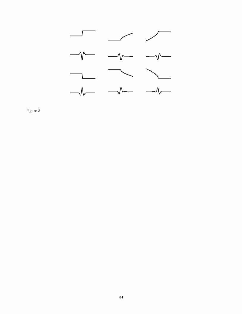
figure 3

34

−0.2 −0.1 0 0.1 0.2 0.3 0.4−0.4

−0.3

−0.2

−0.1

0

0.1

0.2

0.3

0.4α∈ [ 0 1)

−0.2 −0.1 0 0.1 0.2 0.3 0.4−0.4

−0.3

−0.2

−0.1

0

0.1

0.2

0.3

0.4α∈ [ 1 2)

−0.2 −0.1 0 0.1 0.2 0.3 0.4−0.4

−0.3

−0.2

−0.1

0

0.1

0.2

0.3

0.4α∈ [ 2 3)

−0.2 −0.1 0 0.1 0.2 0.3 0.4−0.3

−0.2

−0.1

0

0.1

0.2α∈ [ 3 4)

−0.5 0 0.5−0.4

−0.3

−0.2

−0.1

0

0.1

0.2

0.3

0.4τ∈ [ −π −π/2 1)

−0.5 0 0.5−0.4

−0.3

−0.2

−0.1

0

0.1

0.2

0.3

0.4τ∈ [ −π/2 0)

−0.5 0 0.5−0.4

−0.3

−0.2

−0.1

0

0.1

0.2

0.3

0.4τ∈ [ 0 π/2)

−0.5 0 0.5−0.4

−0.3

−0.2

−0.1

0

0.1

0.2

0.3

0.4τ∈ [ π/2 π)

figure 4

35

0 0.2 0.4 0.6 0.8 1

−1

−0.5

0

0.5

1

(a) Synthetic Seismic Signal

d

0 0.2 0.4 0.6 0.8 1−1

0

1

2

3

4

5

6

7

8

time

(d) Time−Scale Plane: BP0 0.2 0.4 0.6 0.8 1

−1

0

1

2

3

4

5

6

7

8(b) Time−Scale Plane: MOF

0 0.2 0.4 0.6 0.8 1−1

0

1

2

3

4

5

6

7

8

time

scal

e(c) Time−Scale Plane: MP

figure 5

36

0 0.2 0.4 0.6 0.8 1

−1

−0.5

0

0.5

1

(a) Noisy data (SNR=0 db)

d

0 0.2 0.4 0.6 0.8 1−1

0

1

2

3

4

5

6

7

8(d) Time−Scale Plane: BP

0 0.2 0.4 0.6 0.8 1−1

0

1

2

3

4

5

6

7

8

time

(b) Time−Scale Plane: MOF

0 0.2 0.4 0.6 0.8 1−1

0

1

2

3

4

5

6

7

8

time

scal

e

(c) Time−Scale Plane: MP

0 0.1 0.2 0.3 0.4 0.5 0.6 0.7 0.8 0.9 1−1

−0.5

0

0.5

1

(a) Recovered: MOF

0 0.1 0.2 0.3 0.4 0.5 0.6 0.7 0.8 0.9 1−1

−0.5

0

0.5

1

(b) Recovered: MP

0 0.1 0.2 0.3 0.4 0.5 0.6 0.7 0.8 0.9 1−1

−0.5

0

0.5

1

(c) Recovered: BP

figure 6

37

0 0.2 0.4 0.6 0.8 1

−1

−0.5

0

0.5

1

(a) Noisy data (SNR=0 db)

d

0 0.2 0.4 0.6 0.8 1−1

0

1

2

3

4

5

6

7

8(d) Time−Scale Plane: BP

0 0.2 0.4 0.6 0.8 1−1

0

1

2

3

4

5

6

7

8

time

(b) Time−Scale Plane: MOF

0 0.2 0.4 0.6 0.8 1−1

0

1

2

3

4

5

6

7

8

time

scal

e

(c) Time−Scale Plane: MP

0 0.1 0.2 0.3 0.4 0.5 0.6 0.7 0.8 0.9 1−1

−0.5

0

0.5

1

(a) Recovered: MOF

0 0.1 0.2 0.3 0.4 0.5 0.6 0.7 0.8 0.9 1−1

−0.5

0

0.5

1

(b) Recovered: MP

0 0.1 0.2 0.3 0.4 0.5 0.6 0.7 0.8 0.9 1−1

−0.5

0

0.5

1

(c) Recovered: BP

figure 7

38

0 0.1 0.2 0.3 0.4 0.5 0.6 0.7 0.8 0.9 1−0.4

−0.3

−0.2

−0.1

0

0.1

0.2

0.3data and reconstructions

dBPMP

0 0.2 0.4 0.6 0.8 1

−0.2

0

0.2

Amplitude attribute

0 0.2 0.4 0.6 0.8 1

2

4

6

8Scale attribute

0 0.2 0.4 0.6 0.8 1

1

2

3Order attribute

dBPMP

0 0.2 0.4 0.6 0.8 1

−2

0

2

Phase attribute

figure 8

39

0 0.1 0.2 0.3 0.4 0.5 0.6 0.7 0.8 0.9 1−0.15

−0.1

−0.05

0

0.05

0.1

0.15

0.2data and reconstructions

dBPMP

0 0.2 0.4 0.6 0.8 1

−0.2

0

0.2

Amplitude attribute

0 0.2 0.4 0.6 0.8 1

2

4

6

8Scale attribute

0 0.2 0.4 0.6 0.8 1

1

2

3Order attribute

dBPMP

0 0.2 0.4 0.6 0.8 1

−2

0

2

Phase attribute

figure 9

40

0 0.1 0.2 0.3 0.4 0.5 0.6 0.7 0.8 0.9 1−0.2

−0.1

0

0.1

0.2data and reconstructions

dBPMP

0 0.2 0.4 0.6 0.8 1

−0.2

0

0.2

Amplitude attribute

0 0.2 0.4 0.6 0.8 1

2

4

6

8Scale attribute

0 0.2 0.4 0.6 0.8 1

1

2

3Order attribute

dBPMP

0 0.2 0.4 0.6 0.8 1

−2

0

2

Phase attribute

figure 10

41

0 0.1 0.2 0.3 0.4 0.5 0.6 0.7 0.8 0.9 1−0.2

−0.1

0

0.1

0.2data and reconstructions

dBPMP

0 0.2 0.4 0.6 0.8 1

−0.2

0

0.2

Amplitude attribute

0 0.2 0.4 0.6 0.8 1

2

4

6

8Scale attribute

0 0.2 0.4 0.6 0.8 1

1

2

3Order attribute

dBPMP

0 0.2 0.4 0.6 0.8 1

−2

0

2

Phase attribute

figure 11

42

Orignal data

10 20 30 40

50

100

150

200

MP Amplitudes

10 20 30 40

50

100

150

200

BP Amplitudes

10 20 30 40

50

100

150

200

25 30 35 40

0

20

40

60

80

Zoom Orignal data

25 30 35 40

0

20

40

60

80

Zoom MP Amplitudes

25 30 35 40

0

20

40

60

80

Zoom BP Amplitudes

figure 12

43

Original image

50 100 150 200 250 300 350 400 450 500

50

100

150

200

250

300

350

400

450

500−2

−1.5

−1

−0.5

0

0.5

1

1.5

2x 10

−3 Reconstructed image with natom = 25

50 100 150 200 250 300 350 400 450 500

50

100

150

200

250

300

350

400

450

500−2

−1.5

−1

−0.5

0

0.5

1

1.5

2x 10

−3

Estimated amplitudes

Trace #

dept

h

100 200 300 400 500

50

100

150

200

250

300

350

400

450

500−2

−1.5

−1

−0.5

0

0.5

1

1.5

2x 10

−3 Estimated orders

Trace #de

pth

100 200 300 400 500

50

100

150

200

250

300

350

400

450

5000

1

2

3

4

5

6

Estimated scales

Trace #

dept

h

100 200 300 400 500

50

100

150

200

250

300

350

400

450

500

1

2

3

4

5

6

7

Estimated directions

Trace #

dept

h

100 200 300 400 500

50

100

150

200

250

300

350

400

450

5000

0.5

1

1.5

2

2.5

3

3.5

4

50 100 150 200 250 300 350 400 450 500−4

−2

0

2x 10

−3

ReconstructionOriginal

50 100 150 200 250 300 350 400 450 500−5

0

5x 10

−3

50 100 150 200 250 300 350 400 450 500−5

0

5

10x 10

−3

depth

figure 13

44