A

g

r

ect

west

back-

ectral

tions’

erved

TRA

is due

nge

ariabil-

z.

an on

tical-

Seismic background noise along the RISTR

array of broadband seismic stations extendin

from west Texas to southeast Utah

by Joseph Leon

Abstract An analysis of the seismic background noise (SBN) recorded by a temporary linea

array of broadband seismographic stations belonging to the Rio Grande Rift Seismic Trans

(RISTRA) experiment was done. Project RISTRA is a collaboration by research institutions

which will study teleseismic data recorded by a linear array of seismic stations spanning the

Texas Great Plains, the middle Rio Grande Rift and the southern Colorado Plateau. Seismic

ground noise levels at each station is characterized by taking the mean of multiple power sp

densities (PSDs) of representative samples of the total SBN at a station over time. The sta

average PSD of the ambient noise is compared to the mean PSD of the seismic noise obs

across the entire array, allowing inferences to be made regarding relative noise levels at RIS

stations. Results show a high degree of variability in noise levels across the transect. This

probably to the variability in site conditions. Relatively high noise levels in the 1.0 -10 Hz ra

are observed at all of the Great Plains sites as well as the Rio Grande Rift stations. Little v

ity is seen in the SBN across the array in the microseismic frequency range of 0.07 to 0.2 H

Overall, long-period (0.003 - 0.03 Hz) noise is greater on the two horizontal components th

the vertical components, although there is greater variability in long-period noise on the ver

d

te.

fer-

o quan-

ding

h

)

y of

or by

s-

e most

er-

smic

component. The Great Plains stations show the least amount of variability in the long-perio

band.

Introduction

Seismic data are influenced in part by the signal to noise ratio (SNR) at the recording si

Characterizing the seismic background noise (SBN) at seismic recording stations allows in

ences to be made about the quality of data from particular events. Studies have been done t

tify the SBN at sites around the world (Given, 1990; Gurrolaet al., 1990; Given & Fels, 1993;

Peterson, 1993; Liet al., 1994; Stutzmannet al., 2000; Vila, 1998), as well as studies that have

looked at the effects of particular noise sources on SBN (Rodgerset al., 1987; Witherset al.,

1996; Younget al., 1996). Such investigations into SBN have been done for permanent recor

stations with considerable variations in seismometer vault design, for stations equipped wit

downhole sensors, and for temporary stations (like those that house PASSCAL instruments

which typically have sensors on the surface or buried at very shallow depths.

Monitoring the ambient noise conditions at a site is commonly used to determine the utilit

data recorded at seismic stations (Given, 1990; Liet al.,1994). Detectability of seismic events

can be increased by maximizing the SNR at a recording station either by decreasing noise

increasing signal strength (Younget al., 1996). Consequently, when selecting locations for sei

mic stations, one wants to know where the quietest available sites are and how noise can b

effectively minimized at a given site (Younget al., 1996). Many studies of the earth’s internal

structure can be improved by decreasing the noise level, and a good quantification and und

standing of the seismic background noise is the first step in reducing the noise level on sei

data (Stutzmannet al., 2000).

the

992)

may

oise

ern at

d cul-

mper-

ation is

nd

n con-

nd

itions

at the

eak)

IS/

er

In addition to the SBN, a station’s ability to faithfully record seismic events is affected by

noise and distortions within the recording system itself (Rogerset al., 1987). System noise has

been shown to contribute slightly to the background noise at sites investigated by Powell (1

and by Rogerset al. (1987). They found that although some observed high frequency spikes

be due to unknown vibrations of the equipment or to intrinsic seismometer noise, system n

levels are typically well below other sources of noise. However system noise could be a conc

very quiet sites.

Signals from desirable events may be obscured by earth noise arising from both natural an

tural sources. Examples of such noise sources include microseisms, wind, human activity, te

ature changes, and atmospheric pressure changes. In general the seismic noise field at a loc

comprised of body waves, fundamental and higher mode surface waves, and random grou

motions (Powell, 1992). The amount of earth noise encountered is strongly dependent upo

ditions at the recording site (Powell, 1992). Noise can be a function of frequency, location a

time, and is a manifestation of source distribution, propagation effects and receiver site cond

(Powell, 1992).

Cultural noise is an obvious concern at seismic recording stations. Powell (1992) found th

effect of car traffic is to raise spectral levels in the interval of 0.8 - 5.0 Hz (with no obvious p

in shallow deployments of a meter or less. Stutzmannet al.(2000) made similar observations.

Diurnal variations in SBN resulting from human activity patterns have been observed by Liet al.

(1994) and by Stutzmannet al.(2000). Given (1990) observed time-of-day variations at four IR

IDA stations in Eurasia with noise levels during the work day ranging from 1.0 - 14 dB high

than night levels for frequencies above 1.0 Hz.

nted.

ce a sta-

bserv-

in fall

nges

t long

pheric

se on

l.

thers

nd

site.

tly

talla-

ented

e wind

m

Seasonal variations in SBN associated with microseismic activity also have been docume

These effects are seen at varying degrees, depending on site conditions and on the distan

tion is from a shore line (Stutzmann, 2000). It has been found that the microseismic peak, o

able around 0.2 Hz, tends to have a higher amplitude and a shift towards lower frequencies

and winter than in spring and summer (Stutzmannet al., 2000; Vila, 1998; Given, 1990; Rodgers

et al., 1987).

Below 0.1 Hz, noise levels are predominantly influenced by thermal and barometric cha

(Given, 1990). Temperature fluctuations and tilt can cause an increase in horizontal noise a

periods (Given and Fels, 1993). Long-period noise also arises when changes in local atmos

pressure produce ground motion. Such ground motions can be a source of long period noi

the vertical component (Stutzmannet al., 200). Vila (1998) noted a clear correlation between

noise amplitude spectra and atmospheric pressure in the long periods. Stutzmannet al. (2000)

attributed noise in the period band of 20 -100 seconds to atmospheric perturbations as wel

A strong correlation has been shown between wind speed and SBN levels (Vila, 1998; Wi

et al., 1996; Younget al., 1996). The absence of objects that couple wind energy to the grou

(such as trees and man-made structures) is an important consideration in selecting a quiet

Younget al. (1996) report that wind-generated noise is broadband (15 - 60 Hz) and apparen

nonlinear, increasing dramatically when a wind speed threshold is exceeded. At surface ins

tions the minimum wind speeds at which the SBN appears to be influenced has been docum

to be 3 - 4 m/s by Younget al. (1996), 3 m/s by Witherset al. (1996), and 4 - 5 m/s by Gurrolaet

al. (1990). It has been demonstrated that placing a seismometer at depth greatly reduces th

effects. The greatest gains in wind noise reduction appear to be realized within the first 100

(probably less than 10 meters) (Younget al., 1996; Witherset al.,1996).

e tem-

on-

ch

ach

ct is

te

Ala-

ding

Table

tions

n/

ipped

nter.

h they

e

sec-

he

001;

This study analyzes the SBN in the frequency range of 0.001- 10 Hz, along an extensiv

porary array of broadband seismic stations, in order to characterize the seismic noise envir

ment. Characterization is accomplished by looking at amplitude spectra of samples from ea

component separated into day and night time periods, as well as by looking at the ratio of e

station’s spectra to the overall average of the array. A brief description of the research proje

given first.

Rio Grande Rift Seismic Transect Experiment

The Rio Grande Rift Seismic Transect (RISTRA) experiment is a collaborative research

project undertaken by the New Mexico Institute of Mining and Technology, New Mexico Sta

University, the University of Texas at Austin, Dinè College (Shiprock, NM campus) and Los

mos National Laboratory. Project RISTRA employs a passive-source array of seismic recor

stations designed to collect teleseismic data. Station coordinates and elevations are listed in

1 of the appendix. The array became fully operational in November, 1999, although some sta

began recording data as early as July, 1999 ( see Table 3 of appendix for station installatio

removal dates). The main line of the array consists of 54 stations, spaced ~18 km apart, equ

with three-component broadband seismometers on loan from the PASSCAL instrument ce

Stations on the main line are named by using the abbreviation of the respective state in whic

lie, followed by a number from 1 to 54. The numbering begins in the southeastern part of th

transect at TX01 and continues sequentially toward the northwestern-most station, UT54. A

ond line made up of three stations (MB01, MB04(b) & MB05) lies parallel to the main line. T

location of each station is shown in Figure 1. Half of the stations were removed in March 2

the remaining half, in May 2001.

-westn the

s rel-

active

er

the

. The

is the

e con-

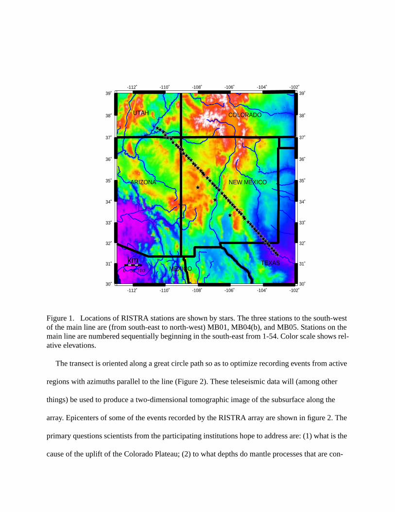
Figure 1. Locations of RISTRA stations are shown by stars. The three stations to the southof the main line are (from south-east to north-west) MB01, MB04(b), and MB05. Stations omain line are numbered sequentially beginning in the south-east from 1-54. Color scale showative elevations.

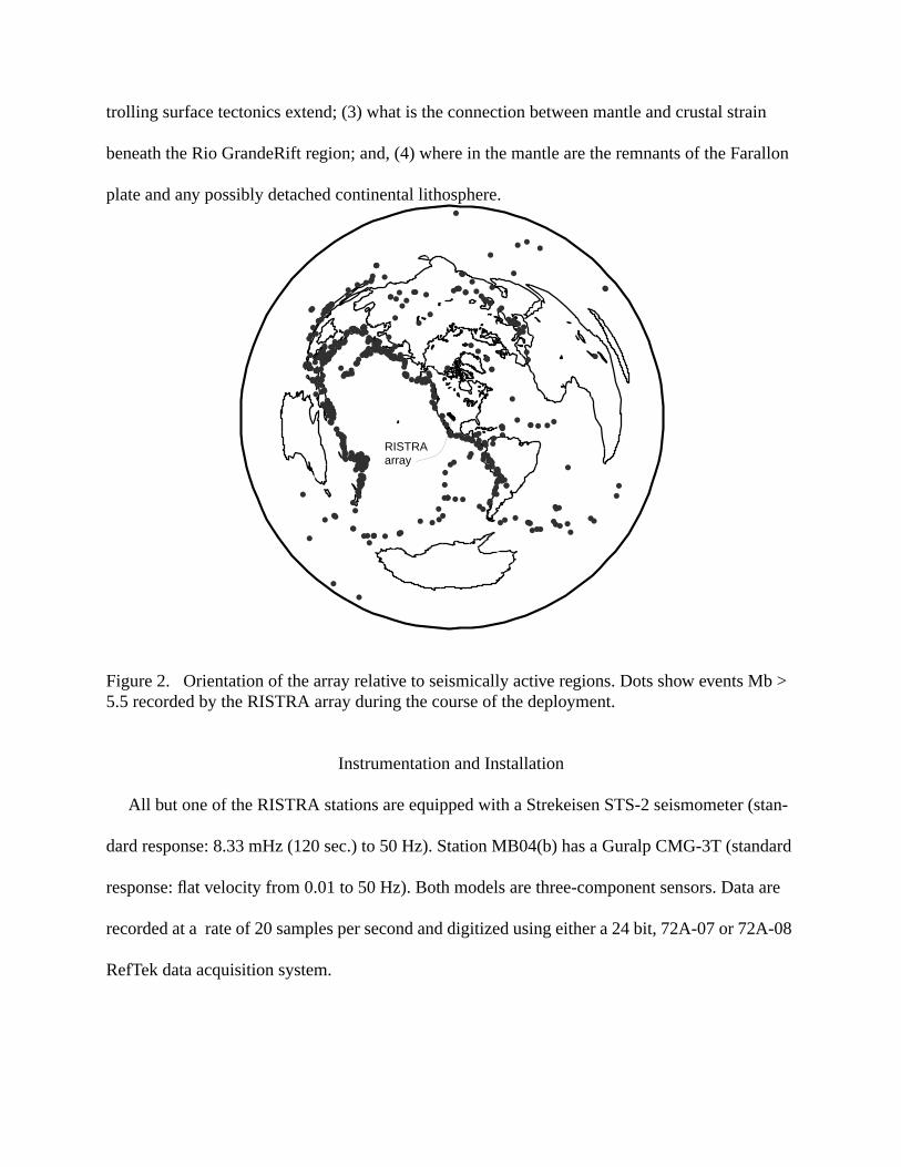
The transect is oriented along a great circle path so as to optimize recording events from

regions with azimuths parallel to the line (Figure 2). These teleseismic data will (among oth

things) be used to produce a two-dimensional tomographic image of the subsurface along

array. Epicenters of some of the events recorded by the RISTRA array are shown in figure 2

primary questions scientists from the participating institutions hope to address are: (1) what

cause of the uplift of the Colorado Plateau; (2) to what depths do mantle processes that ar

-112˚

-112˚

-110˚

-110˚

-108˚

-108˚

-106˚

-106˚

-104˚

-104˚

-102˚

-102˚

30˚ 30˚

31˚ 31˚

32˚ 32˚

33˚ 33˚

34˚ 34˚

35˚ 35˚

36˚ 36˚

37˚ 37˚

38˚ 38˚

39˚ 39˚

0 50 100

km

COLORADOUTAH

ARIZONA NEW MEXICO

TEXASMEXICO

ain

rallon

b >

(stan-

dard

a are

A-08

trolling surface tectonics extend; (3) what is the connection between mantle and crustal str

beneath the Rio GrandeRift region; and, (4) where in the mantle are the remnants of the Fa

plate and any possibly detached continental lithosphere.

Figure 2. Orientation of the array relative to seismically active regions. Dots show events M5.5 recorded by the RISTRA array during the course of the deployment.

Instrumentation and Installation

All but one of the RISTRA stations are equipped with a Strekeisen STS-2 seismometer

dard response: 8.33 mHz (120 sec.) to 50 Hz). Station MB04(b) has a Guralp CMG-3T (stan

response: flat velocity from 0.01 to 50 Hz). Both models are three-component sensors. Dat

recorded at a rate of 20 samples per second and digitized using either a 24 bit, 72A-07 or 72

RefTek data acquisition system.

RISTRAarray

e sen-

wood

ulate

e sites

ivities

le 2

ch sta-

h RIS-

e,

ust,

were

M

In order to minimize thermally induced noise, by maintaining a constant temperature, th

sors are placed about 2 feet below the surface on a concrete pad, in either an insulated ply

vault or a styrofoam vault. About 2 feet of dirt is mounded on top of the vaults to further ins

them (Fig. 3).

Figure 3. Two vault designs used in the RISTRA array.

The array spans a range of geologic as well as topographic and vegetation settings. Som

are fairly remote and isolated from potential noise sources, others are near such cultural act

as rail and road traffic, gas and oil drilling and transportation, ranching, and agriculture. Tab

(appendix) summarizes the site conditions and local potential noise source concerns for ea

tion. Figure 4 depicts the large scale geological setting of the array.

Noise Analysis

An average power spectral density (PSD) of the background noise was calculated for eac

TRA station. “Quiet” (night time, between 2300 -0200 local time) and "noisy" periods (day tim

from 1100-1400 local time) were sampled from each month of data collected between Aug

1999 and November, 2000. Preliminary determination of epicenters reported by the NEIC

referred to in selecting each sample according to the following criteria: (1) no earthquake withb

concrete pad

soil~2 ft

styrofaom

sensor

styr

ofa

om

styrofa

om

ground level

29 In.

2 ft.

4 "

4 "

1.5 " concrete pad

2" pink board insulation

2" pink board insulation

groundlevel

soil~2 ft

sensor

2 ft.

2 ft.

3/4 " plywood

nsure

cutting

noisy"

ieval

The

as the

e three-

Files

’s of

ge sta-

ime

calcu-

tion

y were

is

rom

> 6.0 is reported in the past 24 hours; (2) no earthquake with Mb > 5.0 reported from a distance <

70 degrees from the array in the past day; (3) no earthquake with Mb > 4.0 reported < 20 degrees

away from the array in the previous 12 hours; (4) no earthquake with Mb >3.0 reported <15

degrees away from the array in the previous 3 hours. Samples were visually inspected to e

that earthquake events had been excluded. Electronic spikes and glitches were removed by

them out of the samples when present.

An attempt was made to sample at least three hours of "quiet" time and three hours of "

time from each month per station during the sampling period. Due to two different data retr

methods the noise samples were obtained as files of either 3-hour or one-hour time series.

one-hour files are taken consecutively from the same three hour "noisy" and "quiet" periods

three-hour samples (there are just three one-hour files sampling the same time period as on

hour sample). The sample files from August, 1999 through July, 2000 are 3 hours in length.

from August, 2000 through November, 2000 are one hour long each, but still cumulatively

achieve the same sampling frequency as the three-hour samples.

Noise conditions at each RISTRA station are characterized by taking the mean of the PSD

all data samples collected from each station and comparing them to an array average. Avera

tion noise levels are determined by taking the mean of the PSD’s from both day and night t

samples combined. Separate day ("noisy") time and night ("quiet") time averages also were

lated. A mean background noise PSD for the entire array was calculated from individual sta

averages. Ratios of station mean spectra to the array mean spectra as a function of frequenc

calculated for each station.

The number of sample files used in calculating the average PSD of each station’s SBN

shown in figure A1 (appendix). The variability in the number of files used per station results f

prob-

on seis-

nds

The

od-

the amount of data that met the criteria caused by station down time and other equipment

lems -- and because files of two different lengths were used.

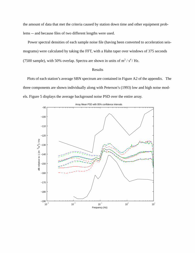
Power spectral densities of each sample noise file (having been converted to accelerati

mograms) were calculated by taking the FFT, with a Hahn taper over windows of 375 seco

(7500 sample), with 50% overlap. Spectra are shown in units of m2 / s4 / Hz.

Results

Plots of each station’s average SBN spectrum are contained in Figure A2 of the appendix.

three components are shown individually along with Peterson’s (1993) low and high noise m

els. Figure 5 displays the average background noise PSD over the entire array.

10−3

10−2

10−1

100

101

−190

−180

−170

−160

−150

−140

−130

−120

−110

−100

−90Array Mean PSD with 95% confidence intervals

Frequency (Hz)

dB

re

lativ

e to

1 (

m2/s

4)

/ H

z

Z−component N−component E−component noise models

95%n.

po-

e isori-

Figure 5. Mean PSD of entire RISTRA array. Each component is shown with its respective confidence interval. Z-component is red, north-component is blue, east-component is greePeterson’s (1993) low and high noise models are in black.

Array-wide day and night time mean spectral levels are plotted for each of the three com

nents in figure 6.

Figure 6 (a). Mean day and night time Z-component SBN PSD’s for the entire array. Day timin blue. Night time is in green. Peterson’s (1993) low and high noise models are in black. Hzontal axis is frequency (Hz). Vertical axis is dB relative to 1 m2/sec.4/Hz.

10−3

10−2

10−1

100

101

−190

−180

−170

−160

−150

−140

−130

−120

−110

−100

−90Z−component array mean day and night spectra with 95% confidence intervals

day night noise models

time Hori-

Figure 6 (b). Mean day and night time north-component SBN PSD’s for the entire array. Dayis in blue. Night time is in green. Peterson’s (1993) low and high noise models are in black.zontal axis is frequency (Hz). Vertical axis is dB relative to 1 m2/sec.4/Hz.

10−3

10−2

10−1

100

101

−190

−180

−170

−160

−150

−140

−130

−120

−110

−100

−90N−component array mean day and night spectra with 95% confidence intervals

day night noise models

10−3

10−2

10−1

100

101

−190

−180

−170

−160

−150

−140

−130

−120

−110

−100

−90E−component array mean day and night spectra with 95% confidence intervals

day night noise models

time Hori-

array

rep-

ctive

level

yellow

re

Figure 6 (c). Mean day and night time north-component SBN PSD’s for the entire array. Dayis in blue. Night time is in green. Peterson’s (1993) low and high noise models are in black.zontal axis is frequency (Hz). Vertical axis is dB relative to 1 m2/sec.4/Hz.

Surface plots of the ratios of the mean spectra for each station to the mean spectra for the

as a function of frequency are given in figure 7 in which a single bar (or column) on the graph

resents the plot of the station mean PSD / array mean PSD ratio vs. frequency of the respe

station. The color scale is logarithmic, thus a ratio around 1.0 indicates a mean station noise

close to the array average. Noise levels greater than the array mean show up as peaks of

and red. Darker blues (ratio < 1.0) indicate frequencies at which the stations’ noise levels a

below the array mean.

traM13

ions.04

Figure 7 (a). Surface plot of the stations’ vertical-component mean background noise specshown as a function of frequency. Note the frequency and the color bar are log scale. TX01-Nare the Plains stations, NM27-NM33 are the Rift stations. NM37-UT54 are the Plateau statThe MB stations are the offline stations.Note station MB03 in the figure is actually MB04; MBon the figure is actually station MB04b. Vertical axis is frequency (Hz).

−10 −5 0 5 10 15

0.01

0.1

1

10

MB

05

MB

04

MB

03

MB

01

UT

54

UT

53

UT

52

UT

51

AZ

50

AZ

49

AZ

48

AZ

47

AZ

46

AZ

45

NM

44

NM

43

NM

42

NM

41

NM

40

NM

39

NM

38

NM

37

NM

36

NM

35

NM

34

NM

33

NM

32

NM

31

NM

30

Z−component background noise ratios

NM

29

NM

28

NM

27

NM

26

NM

25

NM

24

NM

23

NM

22

NM

21

NM

20

NM

19

NM

18

NM

17

NM

16

NM

15

NM

14

NM

13

NM

12

NM

11

NM

10

NM

09

NM

08

NM

07

color scale is log10 ( station mean spectra / array mean )

TX

06

TX

05

TX

04

TX

03

TX

02

TX

01

hown are. The on

Figure 7 (b). Surface plot of the stations’ north-component mean background noise spectra sas a function of frequency. Note the frequency and the color bar are log scale. TX01-NM13the Plains stations, NM27-NM33 are the Rift stations. NM37-UT54 are the Plateau stationsMB stations are the offline stations.Note station MB03 in the figure is actually MB04; MB04the figure is actually station MB04b. Vertical axis is frequency (Hz).

−10 −5 0 5 10 15

0.01

0.1

1

10

MB

05

MB

04

MB

03

MB

01

UT

54

UT

53

UT

52

UT

51

AZ

50

AZ

49

AZ

48

AZ

47

AZ

46

AZ

45

NM

44

NM

43

NM

42

NM

41

NM

40

NM

39

NM

38

NM

37

NM

36

NM

35

NM

34

NM

33

NM

32

NM

31

NM

30

N−component background noise ratios

NM

29

NM

28

NM

27

NM

26

NM

25

NM

24

NM

23

NM

22

NM

21

NM

20

NM

19

NM

18

NM

17

NM

16

NM

15

NM

14

NM

13

NM

12

NM

11

NM

10

NM

09

NM

08

NM

07

color scale is log10 ( station mean spectra / array mean )

TX

06

TX

05

TX

04

TX

03

TX

02

TX

01

hown are. The on

.Figure 7 (c). Surface plot of the stations’ north-component mean background noise spectra sas a function of frequency. Note the frequency and the color bar are log scale. TX01-NM13the Plains stations, NM27-NM33 are the Rift stations. NM37-UT54 are the Plateau stationsMB stations are the offline stations.Note station MB03 in the figure is actually MB04; MB04the figure is actually station MB04b. Vertical axis is frequency (Hz).

−10 −5 0 5 10 15

0.01

0.1

1

10

MB

05

MB

04

MB

03

MB

01

UT

54

UT

53

UT

52

UT

51

AZ

50

AZ

49

AZ

48

AZ

47

AZ

46

AZ

45

NM

44

NM

43

NM

42

NM

41

NM

40

NM

39

NM

38

NM

37

NM

36

NM

35

NM

34

NM

33

NM

32

NM

31

NM

30

E−component background noise ratios

NM

29

NM

28

NM

27

NM

26

NM

25

NM

24

NM

23

NM

22

NM

21

NM

20

NM

19

NM

18

NM

17

NM

16

NM

15

NM

14

NM

13

NM

12

NM

11

NM

10

NM

09

NM

08

NM

07

color scale is log10 ( station mean spectra / array mean )

TX

06

TX

05

TX

04

TX

03

TX

02

TX

01

tions’

y the

d by

z fre-

te per-

cul-

lated

e 7)

elds,

sites

M27

ow-

33)

ly

placed

vity

cated

restric-

ay

A generalized geologic cross-section showing known geologic features as well as the sta

proximity to urban areas is provided in figure 8.

Discussion

The results reveal a large amount of variability in the SBN levels on the data recorded b

RISTRA array. The greatest variability is seen in the higher frequencies (1.0 -10 Hz), followe

the longer periods (0.003 -.03 Hz). The least amount of variation is seen in the 0.07 - 0.2 H

quency range, which contains the microseismic frequencies.

Due to experimental design such as station spacing, array linearity, and to the need for si

mission from land owners/managers little leeway in station placement was afforded. Hence

tural effects contribute greatly to the variability in the higher frequencies. The sites most iso

from such activity show up well in the 1.0 -10 Hz range as dark blue in the ratio plots (Figur

The Great Plains stations, comprised of TX01 - NM13, are located in and around oil/gas fi

significant agricultural activity, and urban areas. Figure 7 reveals higher noise levels at these

relative to the overall array average levels. High frequency noise levels at stations NM14 - N

are lower, to slightly higher than average. NM27 is very isolated from cultural activity. It is h

ever located on the eastern margin of the Rio Grande Rift. The other Rift stations (NM28 - NM

show very high noise levels in the 1.0 - 10 Hz range. These sites are located in the relative

densely populated Rio Grande basin and transportation corridor. Sensors at these sites are

on loose, unconsolidated fill material, which combined with the high amount of cultural acti

may contribute to the higher than average noise levels seen in the higher frequencies.

Stations NM34 - UT54 span the Colorado Plateau. The majority of these stations are lo

on the Navajo Nation. Some of these sites were placed, for convenience and due to design

tions, close to paved roads. NM37 - AZ47 are all fairly close to small towns along US highw

y

Z48

es.

par-

io

tside

d

n a

site.

isiest

ttrib-

ivid-

ompo-

om-

he

ly, the

all

666 and other paved roads (highways) on the Navajo Reservation, resulting in the relativel

higher than average high frequency noise levels observed at these stations.

In the higher frequencies the quietest span of stations in the RISTRA array lies between A

and UT54, which are well within the Colorado Plateau as well as being the most remote sit

High frequency SBN at MB04 is among the highest levels in the array. An interesting com

ison can be made between stations MB04 and MB04b. Both stations were located in the R

Grande Rift above the mid-crustal Socorro magma body. MB04 was located on loose soil ou

of the PASSCAL instrument center on the grounds of the New Mexico Institute of Mining an

Technology. It was moved during the course of the experiment to a new location (MB04b) o

concrete pier placed on bedrock at the entrance of a tunnel, about 2 miles from its original

The difference in noise levels between the two is remarkable in that MB04 is among the no

sites in the array and MB04b is among the quietest. The difference in noise levels can be a

uted to the differences in site and vault conditions. Also note in figure 7 as well as in the ind

ual station plots in the appendix (Figure 9) that the long-period noise levels on the north-

component are higher than those on the east-component, suggesting anisotropy.

On average long-period (0.003 -0.03 Hz) noise levels are higher on the two horizontal c

nents than on the vertical (Figure 5). However the variability in long-period noise on the Z-c

ponents is greater than on the horizontal components (Figure A2). Tilt due to settling of t

concrete pad in the vault may be responsible for some of the long-period noise. Interesting

mean long-period noise levels of the array are higher during the night time than the day on

three components. This may be due to temperature and pressure changes.

3

ls of

ely

than

val-

ely

The Great Plains stations show relatively low, long-period noise levels -- except for NM1

which is the northwestern-most of the Plains stations. It has very high long-period noise leve

unknown origin.

Rift stations NM27 and NM28 have widely different site conditions, yet both have relativ

high long-period noise levels. NM27 is located on bed rock some 400 m in elevation higher

NM27 on the eastern margin of the Rio Grande Rift. NM28 is located in the middle of the rift

ley on loose sand, among the highest levels of cultural activity in the array.

The variability in the SBN levels across all frequencies along the RISTRA array most lik

are due to variations in the individual site conditions.

References

Given, H. K. (1990). Variations in broadband seismic noise at IRIS/IDA stations in the

USSR with implications for event detection,Bull. Seism. Soc. Am.80, 2072-2088.

Given, H. K., and J. F. Fels (1993). Site characteristics and ambient ground noise at

IRIS/IDA stations AAK (Ala-archa, Kyrgyzstan) and TLY (Talaya, Russia),Bull.

Seism. Soc. Am.83, 945-953.

Gurrola, H., J. B. Minster, H. Given, F. Vernon, J. Berger, and R. Aster (1990). Analysis

of high-frequency seismic noise in the western United States and eastern Kazakhstan,

Bull. Seism. Soc. Am.80, 951-970.

Li, Y., W. Prothero Jr., C. Thurber, and R. Butler (1994). Observations of ambient noise

and signal coherency on the island of Hawaii for teleseismic studies,Bull. Seism.

Soc. Am.84, 1229-1242.

Peterson, J. (1993). Observations and modeling of seismic background noise, Open-File

Report 93-322, U.S. Department of Interior Geological Survey.

Powell, C. A. (1992). Seismic noise in northcentral North Carolina,Bull. Seism. Soc.

Am. 82, 1889-1909.

Rodgers, P. W., S. R. Taylor, and K. K. Nakanishi (1987). System and site noise in the

regional seismic test network from 0.1 to 20 Hz,Bull. Seism. Soc. Am.77, 663-678.

Stutzmann, E., G. Roult, and L. Astiz (2000). GEOSCOPE station noise levels,Bull.

Seism. Soc. Am.90, 690-701.

Vila, J. (1998). The broadband seismic station CAD (Tunel del Cadi, eastern Pyrenees):

Site characteristics and background noise,Bull. Seism. Soc. Am.88, 297-303.

Withers, M. M., R. C. Aster, C. J. Young, and E.P. Chael (1996). High-frequency analysis

of seismic background noise as a function of wind speed and shallow depth,Bull.

Seism. Soc. Am.86, 1507-1515.

Young, C. J., E. P. Chael, M. M. Withers, and R. C. Aster (1996). A comparison of

high-frequency (>1 Hz) surface and subsurface noise environment at three sites in

the United States,Bull. Seism. Soc. Am.86, 1516-1528.

AppendixTable 1: RISTRA station locations

TABLE 1.

stationlatitude/longitude

elevation(m)

stationlatitude/longitude

elevation(m)

TX01 31.42324-103.10536

750 NM30 34.74281-106.97360

1515

TX02 31.51328-103.10536

765 NM31 34.84911-107.09767

1676

TX03 31.62320-103.32361

831 NM32 34.98072-107.26429

1685

TX04 31.73379-103.4457

833 NM33 35.11066-107.42286

2094

TX05 31.87845-103.60737

873 NM34 35.26884-107.64317

2735

TX06 31.96710-103.70684

899 NM35 35.34481-107.70697

2133

NM07 32.08454-103.83999

966 NM36 35.44526-107.82246

2176

NM08 32.19915-103.97210

886 NM37 35.57755-108.00173

2254

NM09 32.32648-104.11830

893 NM38 35.70233-108.16292

2077

NM10 32.47293-104.26722

929 NM39 35.7926-108.26736

1949

NM11 32.58364-104.40850

974 NM40 35.94505-108.42896

1796

NM12 32.68287-104.50832

1066 NM41 36.03528-108.57034

1718

NM13 32.80279-104.65484

1177 NM42 36.14851-108.71712

1794

NM14 32.90685-104.75940

1219 NM43 36.24956-108.88712

1991

NM15 33.01441-104.90936

1342 NM44 36.42138-108.95827

1921

NM16 33.17406-105.12670

1625 AZ45 36.45520-109.08242

2683

NM17 33.25657-105.17344

1705 AZ46 36.55126-109.22942

2009

NM18 33.40295-105.34096

1624 AZ47 36.63598-109.33321

1752

NM19 33.49127-105.45537

2028 AZ48 36.76064-109.53932

1664

NM20 33.60478-105.59350

2034 AZ49 36.8869-109.69135

1512

NM21 33.73280-105.74460

2000 AZ50 36.97769-109.86372

1469

NM22 33.84036-105.86888

1691 UT51 37.07315-109.99605

1498

NM23 33.95027-106.01240

1813 UT52 37.23478-110.13132

1671

NM24 34.04687-106.11961

1874 UT53 37.34585-110.33107

1291

NM25 34.16698-106.26052

1933 UT54 37.41870-110.50516

1439

NM26 34.26328-106.36329

1854 MB01 33.33631-106.03395

1446

NM27 34.38562-106.52386

1870 MB04 34.07384-106.92015

1414

NM28 34.54034-106.7002

1484 MB04b 34.07091-106.94225

1489

NM29 34.64724-106.84912

1561 MB05 34.66361-108.01137

2143

TABLE 1.

stationlatitude/longitude

elevation(m)

stationlatitude/longitude

elevation(m)

t-iet"nent

Figure A1. Number of files used in calculating station average PSD’s. (a) "noisy" period eascomponent (b) "noisy" period north-component (c) "noisy" period vertical-component (d) "quperiod east-component (e) "quiet" period north-component (f) "quiet’ period vertical-compo

0

5

1 0

1 5

2 0

2 5

3 0

TX

01

TX

02

TX

03

TX

04

TX

05

TX

06

NM

07

NM

08

NM

09

NM

10

NM

11

NM

12

NM

13

NM

14

NM

15

NM

16

NM

17

NM

18

NM

19

NM

20

NM

21

NM

22

NM

23

NM

24

NM

25

NM

26

NM

27

NM

28

NM

29

NM

30

NM

31

NM

32

NM

33

NM

34

NM

35

NM

36

NM

37

NM

38

NM

39

NM

40

NM

41

NM

42

NM

43

NM

44

AZ

45

AZ

46

AZ

47

AZ

48

AZ

49

AZ

50

UT

51

UT

52

UT

53

UT

54

MB

01

MB

04

MB

04

bM

B0

5

nu

mb

er

of

file

s

0

5

1 0

1 5

2 0

2 5

3 0

TX

01

TX

02

TX

03

TX

04

TX

05

TX

06

NM

07

NM

08

NM

09

NM

10

NM

11

NM

12

NM

13

NM

14

NM

15

NM

16

NM

17

NM

18

NM

19

NM

20

NM

21

NM

22

NM

23

NM

24

NM

25

NM

26

NM

27

NM

28

NM

29

NM

30

NM

31

NM

32

NM

33

NM

34

NM

35

NM

36

NM

37

NM

38

NM

39

NM

40

NM

41

NM

42

NM

43

NM

44

AZ

45

AZ

46

AZ

47

AZ

48

AZ

49

AZ

50

UT

51

UT

52

UT

53

UT

54

MB

01

MB

04

MB

04

bM

B0

5

nu

mb

er

of

file

s

0

5

1 0

1 5

2 0

2 5

3 0

TX

01

TX

02

TX

03

TX

04

TX

05

TX

06

NM

07

NM

08

NM

09

NM

10

NM

11

NM

12

NM

13

NM

14

NM

15

NM

16

NM

17

NM

18

NM

19

NM

20

NM

21

NM

22

NM

23

NM

24

NM

25

NM

26

NM

27

NM

28

NM

29

NM

30

NM

31

NM

32

NM

33

NM

34

NM

35

NM

36

NM

37

NM

38

NM

39

NM

40

NM

41

NM

42

NM

43

NM

44

AZ

45

AZ

46

AZ

47

AZ

48

AZ

49

AZ

50

UT

51

UT

52

UT

53

UT

54

MB

01

MB

04

MB

04

bM

B0

5

nu

mb

er

of

file

s

0

5

1 0

1 5

2 0

2 5

3 0

TX

01

TX

02

TX

03

TX

04

TX

05

TX

06

NM

07

NM

08

NM

09

NM

10

NM

11

NM

12

NM

13

NM

14

NM

15

NM

16

NM

17

NM

18

NM

19

NM

20

NM

21

NM

22

NM

23

NM

24

NM

25

NM

26

NM

27

NM

28

NM

29

NM

30

NM

31

NM

32

NM

33

NM

34

NM

35

NM

36

NM

37

NM

38

NM

39

NM

40

NM

41

NM

42

NM

43

NM

44

AZ

45

AZ

46

AZ

47

AZ

48

AZ

49

AZ

50

UT

51

UT

52

UT

53

UT

54

MB

01

MB

04

MB

04

bM

B0

5

nu

mb

er

of

file

s

0

5

1 0

1 5

2 0

2 5

3 0

TX

01

TX

02

TX

03

TX

04

TX

05

TX

06

NM

07

NM

08

NM

09

NM

10

NM

11

NM

12

NM

13

NM

14

NM

15

NM

16

NM

17

NM

18

NM

19

NM

20

NM

21

NM

22

NM

23

NM

24

NM

25

NM

26

NM

27

NM

28

NM

29

NM

30

NM

31

NM

32

NM

33

NM

34

NM

35

NM

36

NM

37

NM

38

NM

39

NM

40

NM

41

NM

42

NM

43

NM

44

AZ

45

AZ

46

AZ

47

AZ

48

AZ

49

AZ

50

UT

51

UT

52

UT

53

UT

54

MB

01

MB

04

MB

04

bM

B0

5

nu

mb

er

of

file

s

0

5

1 0

1 5

2 0

2 5

3 0

TX

01

TX

02

TX

03

TX

04

TX

05

TX

06

NM

07

NM

08

NM

09

NM

10

NM

11

NM

12

NM

13

NM

14

NM

15

NM

16

NM

17

NM

18

NM

19

NM

20

NM

21

NM

22

NM

23

NM

24

NM

25

NM

26

NM

27

NM

28

NM

29

NM

30

NM

31

NM

32

NM

33

NM

34

NM

35

NM

36

NM

37

NM

38

NM

39

NM

40

NM

41

NM

42

NM

43

NM

44

AZ

45

AZ

46

AZ

47

AZ

48

AZ

49

AZ

50

UT

51

UT

52

UT

53

UT

54

MB

01

MB

04

MB

04

bM

B0

5

nu

mb

er

of

file

s

(a) (b)

(c) (d)

(e) (f)