Seismic Assessment Strategies for Masonry...

Seismic Assessment Strategies for Masonry Structures

by

Matthew J. DeJong

Bachelor of Science, Civil & Environmental Engineering (2001) University of California at Davis

Master of Science, Civil & Environmental Engineering (2005)

Massachusetts Institute of Technology

Submitted to the Department of Architecture in partial fulfillment of the requirements for the degree of

Doctor of Philosophy in Architecture: Building Technology

at the

MASSACHUSETTS INSTITUTE OF TECHNOLOGY

June 2009

© 2009 Massachusetts Institute of Technology All rights reserved

Signature of Author . . . . . . . . . . . . . . . . . . . . . . . . . . . . . . . . . . . . . . . . . . . . . . . . . . . . . . . . . . . . . .

Department of Architecture May 1, 2009

Certified by . . . . . . . . . . . . . . . . . . . . . . . . . . . . . . . . . . . . . . . . . . . . . . . . . . . . . . . . . . . . . . . . . . . .

John A. Ochsendorf Associate Professor of Architecture

Thesis Supervisor Accepted by . . . . . . . . . . . . . . . . . . . . . . . . . . . . . . . . . . . . . . . . . . . . . . . . . . . . . . . . . . . . . . . . . . . .

Julian Beinart Professor of Architecture

Chair, Departmental Committee on Graduate Students

Thesis Supervisor . . . . . . . . . . . . . . . . . . . . . . . . . . . . . . . . . . . . . . . . . . . . . . . . . . . . . . . . . . . . . . . .

John A. Ochsendorf Associate Professor

Department of Architecture, MIT Thesis Reader . . . . . . . . . . . . . . . . . . . . . . . . . . . . . . . . . . . . . . . . . . . . . . . . . . . . . . . . . . . . . . . . . . .

John T. Germaine Senior Research Associate

Department of Civil & Environmental Engineering, MIT Thesis Reader . . . . . . . . . . . . . . . . . . . . . . . . . . . . . . . . . . . . . . . . . . . . . . . . . . . . . . . . . . . . . . . . . . .

Thomas Peacock Associate Professor

Department of Mechanical Engineering, MIT

Seismic Assessment Strategies for Masonry Structures

by

Matthew J. DeJong

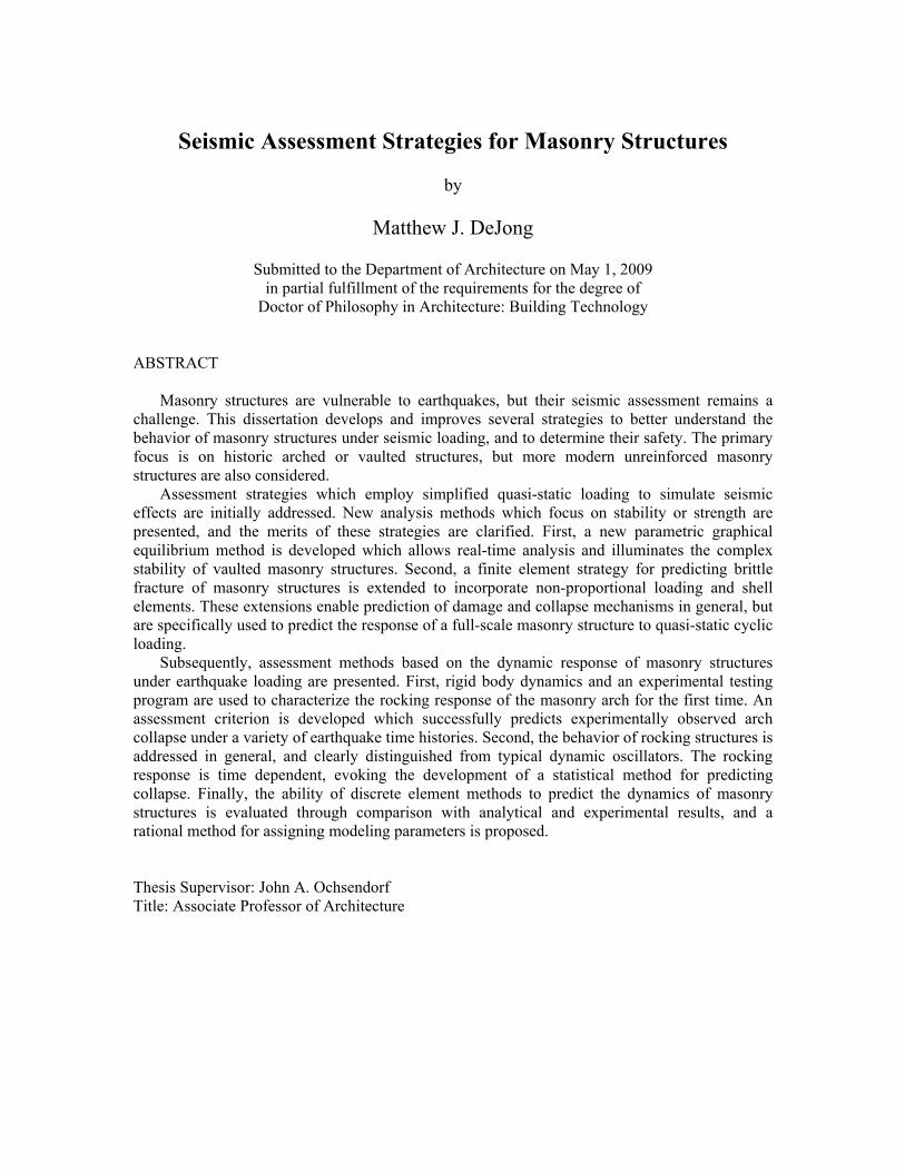
Submitted to the Department of Architecture on May 1, 2009 in partial fulfillment of the requirements for the degree of

Doctor of Philosophy in Architecture: Building Technology ABSTRACT

Masonry structures are vulnerable to earthquakes, but their seismic assessment remains a challenge. This dissertation develops and improves several strategies to better understand the behavior of masonry structures under seismic loading, and to determine their safety. The primary focus is on historic arched or vaulted structures, but more modern unreinforced masonry structures are also considered.

Assessment strategies which employ simplified quasi-static loading to simulate seismic effects are initially addressed. New analysis methods which focus on stability or strength are presented, and the merits of these strategies are clarified. First, a new parametric graphical equilibrium method is developed which allows real-time analysis and illuminates the complex stability of vaulted masonry structures. Second, a finite element strategy for predicting brittle fracture of masonry structures is extended to incorporate non-proportional loading and shell elements. These extensions enable prediction of damage and collapse mechanisms in general, but are specifically used to predict the response of a full-scale masonry structure to quasi-static cyclic loading.

Subsequently, assessment methods based on the dynamic response of masonry structures under earthquake loading are presented. First, rigid body dynamics and an experimental testing program are used to characterize the rocking response of the masonry arch for the first time. An assessment criterion is developed which successfully predicts experimentally observed arch collapse under a variety of earthquake time histories. Second, the behavior of rocking structures is addressed in general, and clearly distinguished from typical dynamic oscillators. The rocking response is time dependent, evoking the development of a statistical method for predicting collapse. Finally, the ability of discrete element methods to predict the dynamics of masonry structures is evaluated through comparison with analytical and experimental results, and a rational method for assigning modeling parameters is proposed. Thesis Supervisor: John A. Ochsendorf Title: Associate Professor of Architecture

Acknowledgements

First, I thank my supervisor, Professor John Ochsendorf, for his guidance and inspiration. The impetus for this research came from his desire to understand the stability of masonry structures, an interest which I have inherited over the last four years. This research was greatly improved by his expertise, and I have thoroughly enjoyed tackling these challenging problems under his mentorship. I can not thank him enough for the opportunities he has provided me, and for truly looking out for my best interests. He has set an example which I hope to emulate in my career.

Second, I acknowledge financial support for this research provided by an MIT Presidential Fellowship, a US Fulbright Pre-Doctoral Grant, and a TU Delft Research Fellowship.

Additionally, I am pleased to acknowledge several others who contributed directly or indirectly to this research. I thank my committee members, Dr. John T. Germaine and Professor Thomas Peacock, for reviewing this work. Specifically, I thank Dr. Germaine for his assistance with the experimental aspects of this research. It has been a privilege working in the company of someone with so much experience and intuition related to physical testing, and someone who is so devoted to helping students succeed.

I am indebted to Professors Jan Rots and Max Hendriks at the Technical University of Delft, for hosting me for one year as a visiting researcher in the Netherlands. I thank them for allowing me to join them in their research regarding finite element analysis of masonry structures, a much needed complement to the rest of the work in this dissertation. Chapter 4 would not have been possible without their expertise. I am also grateful to Professor Andrei Metrikine at the Technical University of Delft, for numerous discussions related to structural dynamics and practically any other subject one could think of. Chapter 6 was inspired by these conversations, which changed the way I perceived the dynamics of rocking structures, and the world. My time working with these colleagues at Delft improved my research, but also changed me personally and encouraged me to pursue an academic career.

I am grateful for collaboration with Laura De Lorenzis of the University of Lecce, Italy, regarding the dynamics of masonry arches in Chapter 5. This effort catalyzed the experimental work on arches, for which I acknowledge the assistance of two undergraduate research students: David Lallemant, who assisted me in constructing a shake table in the Civil Engineering Laboratory, and Stuart Adams, who spent many hours testing masonry arches.

Finally, I would like to thank a few individuals who have shared the last six years at MIT with me. I thank Philippe Block, specifically for his assistance with the thrust line analysis in Chapter 3, but also for numerous conversations related to all aspects of this work. More than that, I thank him for his companionship in our PhD pursuits. I also thank JongMin Shim for his friendship and for exemplifying hard work and endurance in his studies. Most of all, I would like to thank Cara for her enduring support. Her encouragement and enthusiasm made this possible.

9

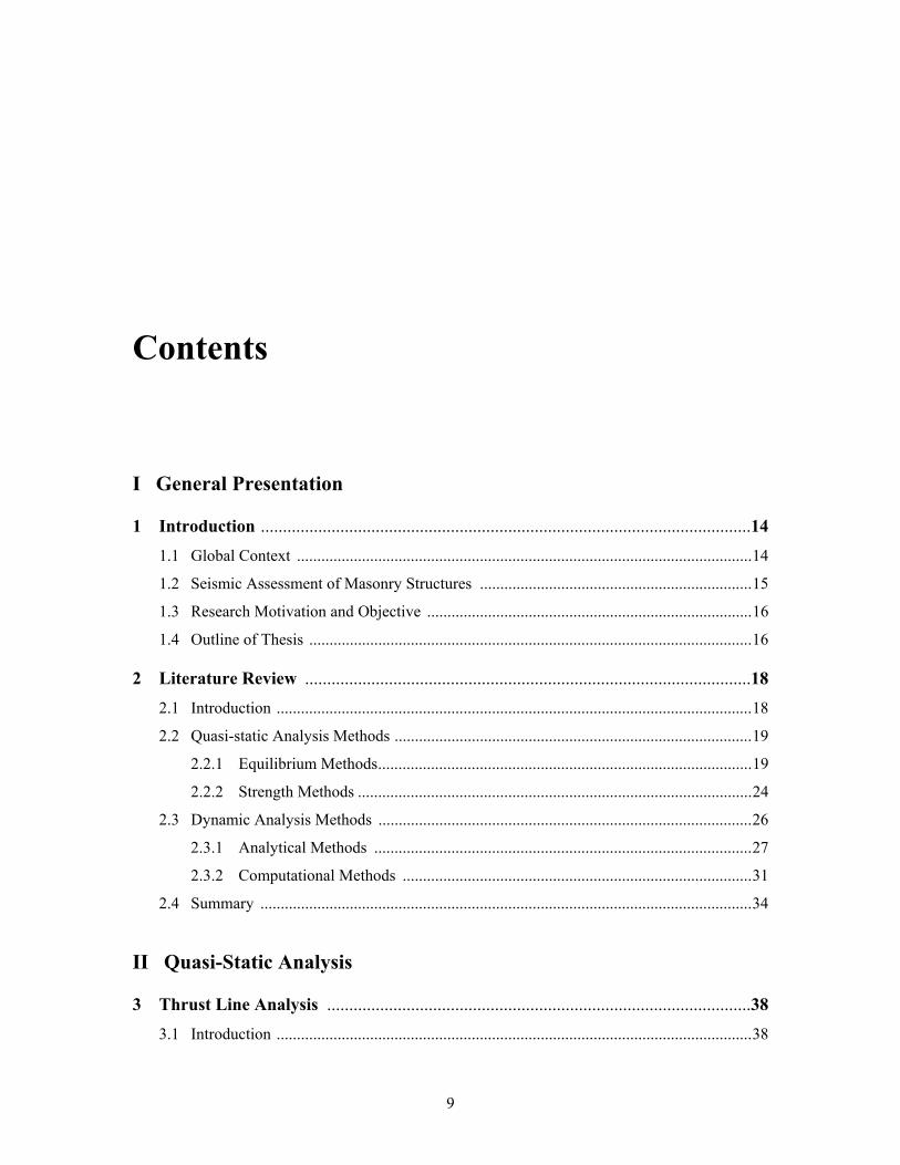
Contents

I General Presentation

1 Introduction ...............................................................................................................14

1.1 Global Context ................................................................................................................14

1.2 Seismic Assessment of Masonry Structures ...................................................................15

1.3 Research Motivation and Objective ................................................................................16

1.4 Outline of Thesis .............................................................................................................16

2 Literature Review .....................................................................................................18

2.1 Introduction .....................................................................................................................18

2.2 Quasi-static Analysis Methods ........................................................................................19

2.2.1 Equilibrium Methods............................................................................................19

2.2.2 Strength Methods .................................................................................................24

2.3 Dynamic Analysis Methods ............................................................................................26

2.3.1 Analytical Methods .............................................................................................27

2.3.2 Computational Methods ......................................................................................31

2.4 Summary .........................................................................................................................34

II Quasi-Static Analysis

3 Thrust Line Analysis ................................................................................................38

3.1 Introduction .....................................................................................................................38

10

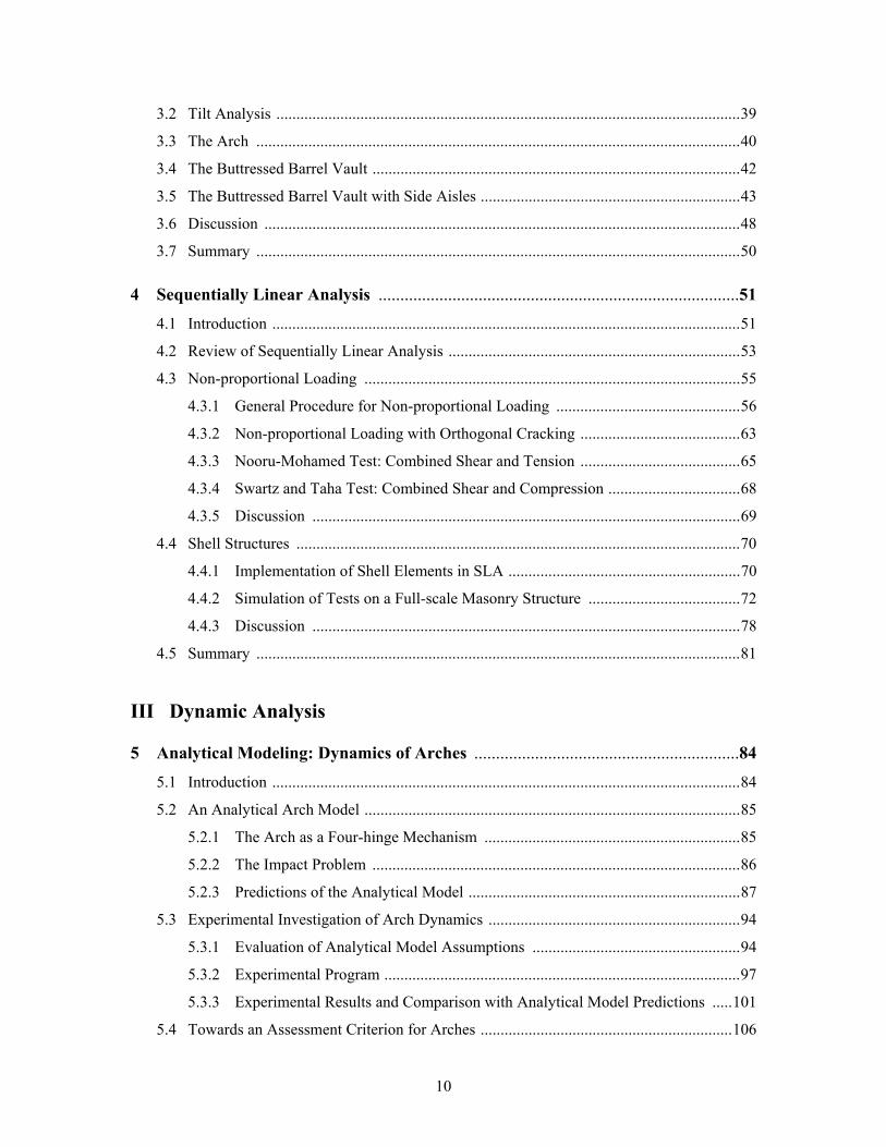
3.2 Tilt Analysis ....................................................................................................................39

3.3 The Arch .........................................................................................................................40

3.4 The Buttressed Barrel Vault ............................................................................................42

3.5 The Buttressed Barrel Vault with Side Aisles .................................................................43

3.6 Discussion .......................................................................................................................48

3.7 Summary .........................................................................................................................50

4 Sequentially Linear Analysis ...................................................................................51

4.1 Introduction .....................................................................................................................51

4.2 Review of Sequentially Linear Analysis .........................................................................53

4.3 Non-proportional Loading ..............................................................................................55

4.3.1 General Procedure for Non-proportional Loading ..............................................56

4.3.2 Non-proportional Loading with Orthogonal Cracking ........................................63

4.3.3 Nooru-Mohamed Test: Combined Shear and Tension ........................................65

4.3.4 Swartz and Taha Test: Combined Shear and Compression .................................68

4.3.5 Discussion ...........................................................................................................69

4.4 Shell Structures ...............................................................................................................70

4.4.1 Implementation of Shell Elements in SLA ..........................................................70

4.4.2 Simulation of Tests on a Full-scale Masonry Structure ......................................72

4.4.3 Discussion ...........................................................................................................78

4.5 Summary .........................................................................................................................81

III Dynamic Analysis

5 Analytical Modeling: Dynamics of Arches .............................................................84

5.1 Introduction .....................................................................................................................84

5.2 An Analytical Arch Model ..............................................................................................85

5.2.1 The Arch as a Four-hinge Mechanism ................................................................85

5.2.2 The Impact Problem ............................................................................................86

5.2.3 Predictions of the Analytical Model ....................................................................87

5.3 Experimental Investigation of Arch Dynamics ...............................................................94

5.3.1 Evaluation of Analytical Model Assumptions ....................................................94

5.3.2 Experimental Program .........................................................................................97

5.3.3 Experimental Results and Comparison with Analytical Model Predictions .....101

5.4 Towards an Assessment Criterion for Arches ...............................................................106

11

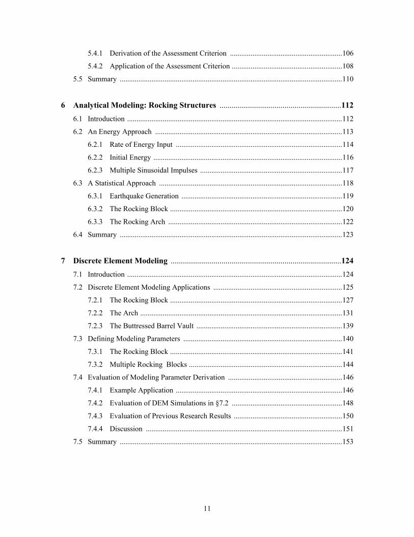
5.4.1 Derivation of the Assessment Criterion ............................................................106

5.4.2 Application of the Assessment Criterion ...........................................................108

5.5 Summary .......................................................................................................................110

6 Analytical Modeling: Rocking Structures ............................................................112

6.1 Introduction ...................................................................................................................112

6.2 An Energy Approach ....................................................................................................113

6.2.1 Rate of Energy Input .........................................................................................114

6.2.2 Initial Energy .....................................................................................................116

6.2.3 Multiple Sinusoidal Impulses ............................................................................117

6.3 A Statistical Approach ..................................................................................................118

6.3.1 Earthquake Generation ......................................................................................119

6.3.2 The Rocking Block ............................................................................................120

6.3.3 The Rocking Arch .............................................................................................122

6.4 Summary .......................................................................................................................123

7 Discrete Element Modeling ....................................................................................124

7.1 Introduction ...................................................................................................................124

7.2 Discrete Element Modeling Applications .....................................................................125


7.2.2 The Arch ............................................................................................................131

7.2.3 The Buttressed Barrel Vault ..............................................................................139

7.3 Defining Modeling Parameters .....................................................................................140


7.3.2 Multiple Rocking Blocks ..................................................................................144

7.4 Evaluation of Modeling Parameter Derivation .............................................................146

7.4.1 Example Application .........................................................................................146

7.4.2 Evaluation of DEM Simulations in §7.2 ...........................................................148

7.4.3 Evaluation of Previous Research Results ..........................................................150

7.4.4 Discussion .........................................................................................................151

7.5 Summary .......................................................................................................................153

12

IV Conclusions

8 Conclusions ..............................................................................................................156

8.1 Summary of Main Findings ..........................................................................................156

8.2 Primary Contributions ...................................................................................................158

8.3 Future Research .............................................................................................................159

V Appendices

A Notation ....................................................................................................................162

B Implementation of the Analytical Arch Model in Matlab ...................................166

B.1 Introduction ..................................................................................................................166

B.2 Additional Details of the Analytical Model .................................................................166

B.3 Implementation in Matlab ...........................................................................................169

C Shake Table Design .................................................................................................172

C.1 Introduction ..................................................................................................................172

C.2 Power, Control, and Data Recording ............................................................................172

C.3 General Layout and Construction Drawings ................................................................173

Bibliography

13

Part I

General Presentation

14

Chapter 1

Introduction

1.1 Global Context

Masonry structures comprise a majority of the global built environment. These structures

exist in the form of typical houses and office buildings, but also include a wealth of invaluable

structures which compose the fabric of human history. Masonry refers to “the art and craft of

building and fabricating in stone, clay, brick, or concrete block” (“masonry”, 2009). In this

dissertation, masonry is used to refer to traditional masonry, often referred to as unreinforced

masonry. The array of structures within this category is vast, ranging from historic stone

structures to mortared brick structures still being constructed today.

Many masonry structures are located in seismic regions, where earthquakes have exposed

their vulnerability. Recent earthquakes in Iran [2003], Pakistan [2005], and Peru [2007] have

caused devastating loss of life and infrastructure. For example, the earthquake in Pakistan killed

more than 80,000 people and left more than 4 million homeless (EERI 2005). The 2003

earthquake in Iran killed 30,000, the majority of whom were buried by collapsing masonry.

Eighty percent of the city of Bam was flattened, including the iconic, 2500 year old citadel

(Fallahi 2007).

This problem is obviously not limited to the developing world. Italy has seen significant

damage to its infrastructure during recent earthquakes, including the collapse of a frescoed vault

in the Basilica of St. Francis of Assisi in 1997 (Bohlen 1997). A wealth of similar damage during

15

recent earthquakes catalyzed an increase in seismic assessment requirements in Italy (Povoledo

2007), motivating an increase in related research in the country. Here in the United States, the re-

evaluation of San Francisco’s infrastructure at the 100 year anniversary of the devastating 1906

earthquake resulted in masonry structures being labeled the highest retrofit priority of all

structural typologies.

Despite their prevalence and their long existence, the behavior of masonry structures under

earthquake loading is still not well understood, and extremely hard to predict. The problem is

challenging and it must be addressed.

1.2 Seismic Assessment of Masonry Structures

Why does it remain difficult to determine the safety of masonry structures in seismic regions?

First, the majority of these structures did not benefit from modern engineering design, but instead

resulted from empirical expertise. As a result, masonry assessment methods have naturally lagged

far behind assessment methods for modern steel and concrete structures.

Second, the long existence of many masonry structures yields several unknowns. In most

cases, geometry is difficult to determine because construction drawings do not exist, and

environmental factors have resulted in material degradation, support displacements, and damage

during extreme events.

Third, the basic nature of masonry remains difficult to model. Finite Element Modeling

(FEM), the most widespread structural analysis tool, is tailored toward continuous structures

which remain relatively connected during elasto-plastic failure under both static and dynamic

loading. Masonry, on the other hand, is discontinuous by nature. Failure is brittle and individual

units (e.g. stones, bricks) are often free to separate, especially during dynamic loading. While

progress has been made towards modeling these behaviors using FEM, alternative methods are

attractive but underdeveloped.

Finally, researchers and engineers remain divided in their emphasis on what is important:

strength or stability. Certainly, the answer is a combination of the two, and largely depends on the

nature of the specific structure. However, the assessment methods applied to these structures

generally emphasize strength, while neglecting stability (Boothby 2001). There is need for

integration of these two concepts, and an understanding for what is critically important.

These difficulties have resulted in a misunderstanding of structural behavior of masonry. In

turn, this has led to unnecessary interventions, and even destructive interventions, which must be

16

prevented in the future. It has also made it difficult to identify which buildings are at risk of

collapse.

1.3 Research Motivation and Objective

As the previous sections mentioned, there is a global need to evaluate the safety of masonry

structures, and there are technical limitations which are preventing this need from being met. This

context provides the general motivation for this work:

• We need a better fundamental understanding of both the static and dynamic behavior of

masonry structures in order to improve assessment methods.

• We need better numerical tools to predict both the quasi-static and the dynamic response

of masonry structures.

Based on these motivating factors, this dissertation aims:

To increase fundamental understanding of structural behavior and to develop

accurate, tested analysis methods that allow appropriate assessment of masonry

structures which are vulnerable to seismic loading.

To meet this objective, a variety of methods will be applied, as outlined in §1.4. These

approaches are tailored to different types of failure (strength -vs- stability), loading (quasi-static -

vs- dynamic), and structures (simple -vs- complex; historic -vs- modern). Analytical, geometrical,

numerical, and experimental approaches are incorporated.

This broad approach is intentional. A wide-ranging exploration of available methods is

necessary to determine the most appropriate method for a given structure. Furthermore, the broad

scope bridges the gap between these methods, showing how they can be complementary. This

work will clarify the state of the field, and push it further in several directions.

1.4 Outline of Thesis

The approach taken to achieve the objective in §1.3 is as follows. Part I includes this

introduction, which states the problem, and Chapter 2, which reviews previous research. The aim

is to set the context for the contributions made in this dissertation.

Part II is focused on quasi-static assessment methods, primarily the modeling of quasi-static

collapse. There is no point in modeling dynamic collapse without first addressing and

understanding the quasi-static problem. Chapter 3 extends the graphical equilibrium assessment

17

method of Thrust Line Analysis, a method purely focused on the stability of masonry, not on

strength. This simple but powerful approach, tailored towards historic vaulted masonry structures,

can be used as a first order assessment method, but is also of educational value as a means of

clarifying the fundamental concept of collapse due to instability.

Chapter 4, on the other hand, deals with predicting damage to masonry structures through the

modeling of failure due to lack of material strength. Methods which were primarily developed to

predict strength failure can give an indication of possible collapse mechanisms, but often struggle

to predict collapse. In Chapter 4, a new method for modeling brittle fracture using finite element

analysis is presented. This method, while applicable to brittle structures in general, is applied

towards relatively modern brick structures with horizontal floor and roof diaphragms and

masonry walls.

Part III is focused on dynamic collapse under earthquake loading. While Part II addressed

both stability and strength, Part III will only address collapse due to instability. This is motivated

by the fact that a majority of research has been devoted to the possibility of elastic resonance,

which might lead to material failure but does not necessarily explain much about collapse. Less

research has been devoted to the dynamic response of discrete interacting masonry blocks which

are assumed to have no tensile strength (i.e. which have no mortar or unreliable mortar strength).

Part III starts with Chapter 5, an analytical and experimental investigation of the masonry

arch under dynamic loading. Despite its prevalence throughout history, dynamic collapse

conditions for the masonry arch have not been defined. In contrast to previous studies regarding

elastic vibrations, the dry-stone arch and other vaulted masonry structures are shown to behave as

rocking structures which must be treated differently than typical elastic structures.

Chapter 6, inspired by the findings in Chapter 5, is focused on the fundamental behavior of

rocking structures. While numerous papers have been written on the single rocking block, certain

aspects of its behavior remain undefined. Specifically, the ground motions to which rocking

structures are most vulnerable are clarified.

While Chapters 5 and 6 are primarily deal with fundamental behavior and analytical

assessment methods, Chapter 7 focuses on numerical modeling. It is impossible to create

analytical models to predict the dynamic response of most full-scale structures, so computational

power must be employed. This chapter explores discrete element modeling, first using it to

predict experimental response of the arch and then applying it to larger scale structures.

Additionally, a method for defining critical modeling parameters is presented.

Part IV summarizes this work and discusses avenues of future research. The conclusions

justify the broad spectrum of approaches discussed throughout.

18

Chapter 2

Literature Review

2.1 Introduction

The safety assessment of masonry structures in seismic regions has gained significant

attention in recent years. Increased computational power has changed the way all kinds of

structures are assessed, allowing more degrees of freedom to be modeled. In this chapter, it is

unrealistic to attempt a comprehensive overview of all methods which have been applied. Instead,

the basic frameworks in which masonry structures are assessed will be introduced, to provide the

context for the contributions herein. This chapter, like the dissertation, is divided into two main

sections: quasi-static analysis and dynamic analysis.

Equilibrium methods, strength methods, discrete block methods, and continuum methods will

be reviewed. While these methods vary dramatically in their assumptions and complexities, the

question should not be “Which method is better?” Instead, realizing that all of these methods are

appropriate for given applications, the questions which should be asked are “How can these

methods be improved?” and “Where can new contributions be made?” The answers to these

questions motivate the work in the following chapters.

19

2.2 Quasi-static Analysis Methods

Quasi-static analysis methods are the logical starting place, as these methods were the first to

be formalized. By neglecting dynamic effects entirely, or by approximating them in a quasi-static

fashion, a first-order seismic assessment is possible, often with reduced computational power,

time, and therefore expense. While more approximate, these methods are powerful and practical,

and remain the primary tools applied to assess masonry structures today.

Dynamic earthquake loading is typically simplified as a quasi-static loading in one of two

ways. The first method is to apply a constant horizontal acceleration to the structure, which is the

equivalent of applying a constant horizontal ground motion. This conservatively ignores the fact

that actual ground motions only occur for a short period of time, but also neglects the possibility

of resonant amplification. Thus, this method is appropriate when stability is a concern and where

elastic resonance is expected to have a relatively small effect, as discussed in §2.2.1.

The second method involves applying horizontal forces distributed along the height of the

structure, which are meant to approximate the effects of an earthquake. The relative magnitudes

of the forces are distributed with preference towards the top of the structure, accounting for

amplification caused by dynamic resonance effects (e.g. Uniform Building Code 1997). All of the

horizontal forces can then be scaled to approximate different magnitude earthquakes, and the

response of the structure can be determined. This concept has been extended into what is typically

referred to as “pushover analysis” (American Society of Civil Engineers 2000). Initially,

pushover analysis was developed for frame-type structures typical of steel and concrete

construction. However, the technique has also been applied to masonry structures by modeling

continuous wall elements directly or through use of the equivalent frame technique. This method

is appropriate for strength methods, where resonance effects may play a larger role and must be

accounted for, as discussed in §2.2.2.

2.2.1 Equilibrium Methods

Equilibrium methods, or stability methods, have been used for centuries (Heyman 1995,

Huerta 2004). Recent studies show that some historic masonry structures were built on the edge

of stability, hinting at the idea of the builder adding more mass or thickness where necessary to

make the structure stand and ensure safety (Nikolinakou et al. 2005). However, this was not

always the case. In the late 19th century, Antoni Gaudi used hanging mass models to develop

stable forms. This design methodology takes advantage of the fact that masonry structures act

20

predominantly in compression. Once Gaudi had established the most efficient form in tension, he

inverted that form to construct a pure compression structure.

Although Gaudi’s hanging models are perhaps more well-known, the idea of pure

compression structures was investigated much earlier. Hooke (1675) wrote, "As hangs the

flexible line, so but inverted will stand the rigid arch." The mathematical solution to the shape of

the hanging chain, the catenary, was later published by Gregory (1697), who states, "...none but

the catenaria is the figure of a true legitimate arch, or fornix. And when an arch of any other

figure is supported, it is because in its thickness some catenaria is included." Heyman (1998)

restates this in a more general sense, "...if any thrust line can be found lying within the masonry,

then the arch will stand."

Based on this foundation, Couplet made three key assumptions about the behavior of

masonry in 1730: (1) masonry has no tensile strength, (2) masonry has infinite compressive

strength, and (3) sliding failure between arch voussoirs does not occur (Heyman 1998). These

assumptions still provide the criteria used for analysis of masonry structures, as outlined by

Heyman (1966, 1995). Furthermore, these assumptions eliminate the possibility of failure due to

material strength, so only failure due to instability can be assessed. Thus, methods which

incorporate these assumptions are referred to as “equilibrium methods” in this thesis. Couplet’s

assumptions have the following consequences:

• The static analysis of masonry structures is a problem of stability which is based solely

on geometry. Analysis results are independent of scale, meaning that a small scale model

should behave the same as a full scale structure.

• Individual blocks are not free to slide or crush, but they are free to separate, or hinge.

Hinges form when the ‘thrust line’ mentioned by Heyman (1998), can no longer be

contained within the masonry and exits the surface of the masonry. At this point, the

masonry can no longer support the applied loads, and the structure is no longer in

equilibrium without hinging.

• Since stresses are not a concern, a constant horizontal acceleration can be achieved by

tilting the ground surface upon which a structure rests. This concept was applied by

researchers at the Institute for Lightweight Structures in Suttgart, Germany, who tilted

model masonry structures until collapse to determine their resistance to lateral loading

(Gaß 1990).

Equilibrium methods are primarily applied to pure compression structures. Thus, they are

more appropriate for historical masonry structures, which incorporate vaults and arches to

transfer loads instead of slabs and beams. Therefore, the discussion and application of

21

equilibrium methods will be limited to these types of structures. These methods have been

implemented in two primary ways: graphically and numerically.

Graphical Equilibrium Methods

Graphical methods have long been used for the design and assessment of masonry structures

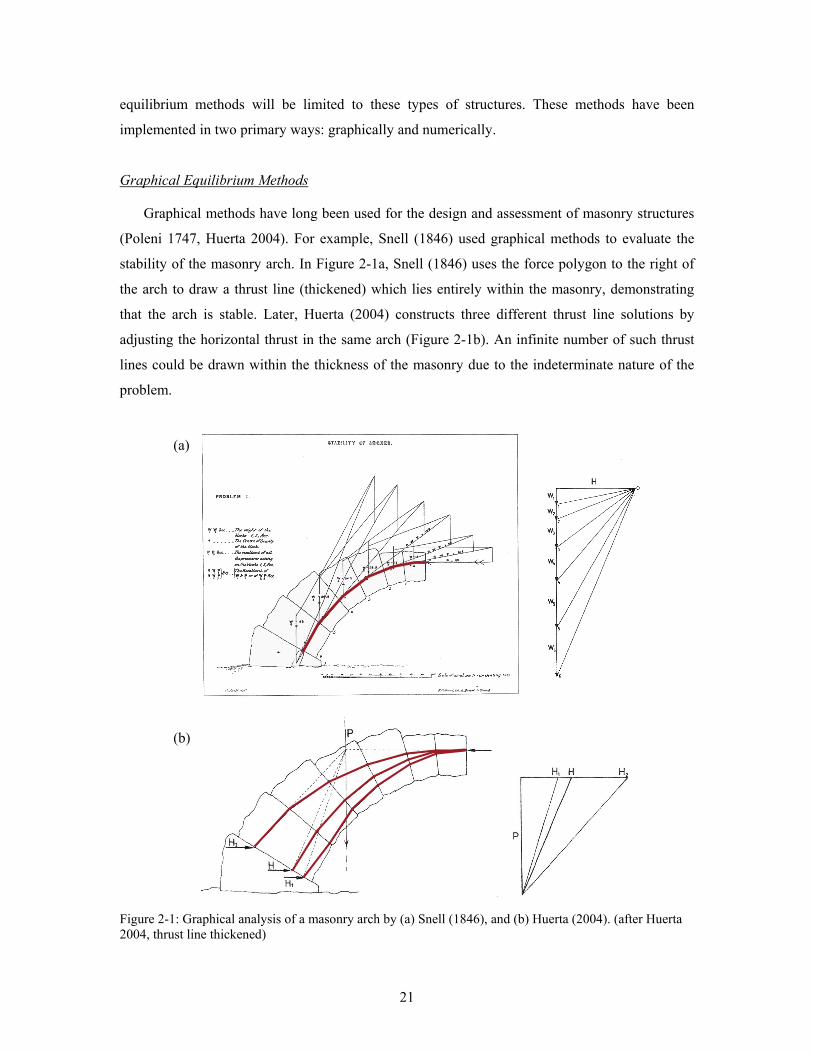
(Poleni 1747, Huerta 2004). For example, Snell (1846) used graphical methods to evaluate the

stability of the masonry arch. In Figure 2-1a, Snell (1846) uses the force polygon to the right of

the arch to draw a thrust line (thickened) which lies entirely within the masonry, demonstrating

that the arch is stable. Later, Huerta (2004) constructs three different thrust line solutions by

adjusting the horizontal thrust in the same arch (Figure 2-1b). An infinite number of such thrust

lines could be drawn within the thickness of the masonry due to the indeterminate nature of the

problem.

Figure 2-1: Graphical analysis of a masonry arch by (a) Snell (1846), and (b) Huerta (2004). (after Huerta 2004, thrust line thickened)

(a)

(b)

22

Perhaps the most widely applied method of graphical analysis is graphic statics, formalized

by Karl Culmann (1866). In recent years, graphical methods have been largely replaced by

numerical methods, especially in engineering education. However, recent work by Allen and

Zalewski (2009) demonstrates that graphic statics is still a viable and powerful technique for both

analysis and design.

One major drawback of graphical methods, which likely led to their reduced application, is

that hand-drawn graphical constructions can be tedious and time-consuming. However, recent

interactive computational geometry software can significantly reduce this negative aspect. By

implementing graphic statics in a parametric computational geometry framework, Block (2005)

developed a useful tool for assessment and design. Using the assumption that stability is based

solely on geometry, Block (2005) developed parametric constructions for various masonry

structures. These constructions are created only once, after which the geometry can be adjusted in

real-time. Using this tool, a rapid first order assessment of the stability of masonry structures can

be achieved, and the effect of geometrical changes such as arch thickness, buttress width, etc., can

be readily evaluated. Furthermore, the visual results often lead to better understanding and clearer

interpretation.

The application of graphical methods to assess the stability of arches under quasi-static

seismic loading has not been attempted. Prior to the computational implementation introduced by

Block (2005), this would have been prohibitively time-consuming.

Numerical Equilibrium Methods

Numerical equilibrium methods have been applied to study the stability of masonry structures

under quasi-static point loads or displacements, but this section will focus on seismic assessment

of arches and vaulted structures. All of these approaches apply a constant horizontal acceleration

to simulate possible earthquake effects, either directly or by tilting the structure.

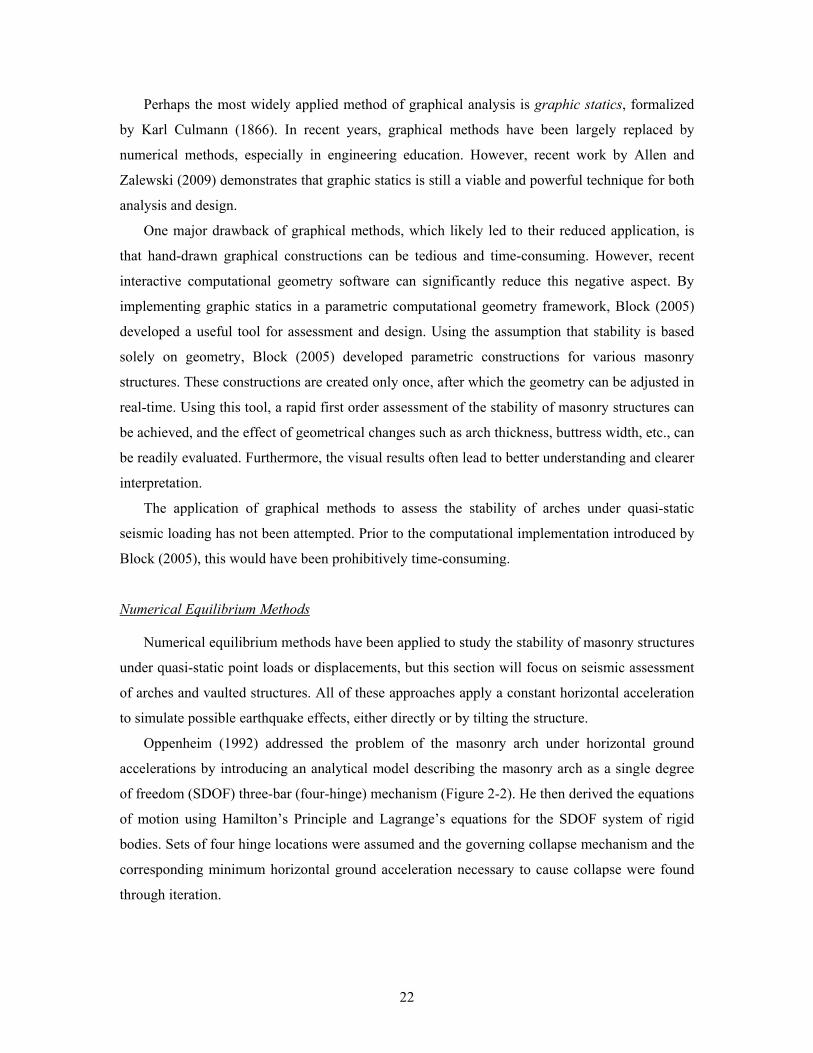
Oppenheim (1992) addressed the problem of the masonry arch under horizontal ground

accelerations by introducing an analytical model describing the masonry arch as a single degree

of freedom (SDOF) three-bar (four-hinge) mechanism (Figure 2-2). He then derived the equations

of motion using Hamilton’s Principle and Lagrange’s equations for the SDOF system of rigid

bodies. Sets of four hinge locations were assumed and the governing collapse mechanism and the

corresponding minimum horizontal ground acceleration necessary to cause collapse were found

through iteration.

23

Figure 2-2: The three bar mechanism formed by a masonry arch under horizontal ground motion. (after Oppenheim 1992)

Clemente (1998) also studied the collapse of a masonry arch subjected to constant horizontal

ground acceleration by assuming four hinge locations and writing the equilibrium equations in

terms of virtual powers. Again by iterating through all the possible sets of hinge locations which

would cause collapse, the governing horizontal ground acceleration was identified, and the

corresponding collapse mechanism was found. Using this procedure, he plotted the constant

horizontal acceleration required to cause collapse as well as the locations of the hinges at the

point of collapse for various arch geometries. Results compare well with the results of

Oppenheim (1992).

Appleton (1999) and Ochsendorf (2002) studied the same problem by using the principle of

virtual work to determine the ground surface tilt which causes collapse, and the corresponding

horizontal ground acceleration. Ochsendorf (2002) extended the analysis to a buttressed arch and

showed the relative effect of both the arch and the buttress on the stability of the structure.

Additionally, Ochsendorf developed a method for determining the cracking of a tilting buttress

which can be observed during collapse. This buttress cracking results directly from the postulate

that the masonry has no tensile strength, and clearly reduces the maximum allowable horizontal

acceleration.

Finally, other authors have extended these ideas to address more complete structures. For

example, De Luca et al. (2004) assessed the stability of an arch on buttresses in a similar fashion.

Additionally, they propose the use of finite element models to determine where cracking of a

masonry structure might occur, and then use equilibrium methods to determine the stability of the

determined mechanism. Essentially, they include some tensile strength to determine a collapse

mechanism, and then neglect the tensile strength when assessing stability. This approach leads the

discussion to methods which incorporate strength.

ADD OPPENHEIM

24

2.2.2 Strength Methods

In some cases, it is not reasonable or desirable to make the three assumptions that are

incorporated in the equilibrium methods discussed in §2.2.1, and the strength of the material

needs to be included in the analysis. This could be the case for newer brick-and-mortar

construction where the tensile strength of mortar is appreciable. Or it could be the case for certain

structural typologies where the structure is confined or constrained so as to prevent instability

without significant sliding or crushing, e.g. for the in-plane failure of masonry walls.

In general, the primary advantage of strength methods is their ability to predict or assess

damage. However, once some of level of damage has been developed, it often remains a

challenge for these methods to predict when the structure will collapse. The basis for strength

methods is vast, ranging from micromechanical modeling of failure to macro-scale approximation

of masonry properties.

Micro-mechanical Damage Models

With an emphasis on micromechanical modeling, Lourenço (1996) outlined computational

strategies for masonry structures, starting with separate brick and mortar layers. This led to the

development of a brick-interface model (Lourenço and Rots 1997) and an anisotropic continuum

model (Lourenço and Rots 1998) for finite element analysis of masonry. Similarly, Gambarotta

and Lagomarsino (1997a) proposed a brick-and-mortar damage model for seismic loading, and

then applied homogenization techniques to develop a continuum model applicable to cyclic

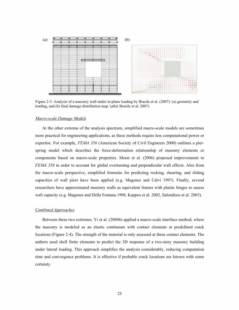
loading of masonry walls (Gambarotta and Lagomarsino 1997b). More recently, Brasile et al.

(2007) built upon this work, developing more efficient iteration techniques for a similar brick-

and-mortar joint model, making this complex micro-scale model more feasible (Figure 2-3).

In addition to these studies focused on the in-plane failure of brick-and-mortar walls, micro-

mechanical models have been applied to assess historic masonry structures. For example, Velente

(2003) used complex fracture mechanics to address the failure and reconstruction of Noto

cathedral, which collapsed following an earthquake in 1996. Additionally, commercially

available homogenized crack models have been widely applied to predict damage to masonry

structures in seismic regions (e.g. Romano 2003). However, the material properties, geometry,

and existing damage of historic structures are often poorly defined. Thus, use of these techniques

should be applied tentatively, with an understanding of the limited level of accuracy which can be

realistically achieved. The majority of methods in this category employ finite element software

for analysis.

25

Figure 2-3: Analysis of a masonry wall under in-plane loading by Brasile et al. (2007): (a) geometry and loading, and (b) final damage distribution map. (after Brasile et al. 2007)

Macro-scale Damage Models

At the other extreme of the analysis spectrum, simplified macro-scale models are sometimes

more practical for engineering applications, as these methods require less computational power or

expertise. For example, FEMA 356 (American Society of Civil Engineers 2000) outlines a pier-

spring model which describes the force-deformation relationship of masonry elements or

components based on macro-scale properties. Moon et al. (2006) proposed improvements to

FEMA 356 in order to account for global overturning and perpendicular wall effects. Also from

the macro-scale perspective, simplified formulas for predicting rocking, shearing, and sliding

capacities of wall piers have been applied (e.g. Magenes and Calvi 1997). Finally, several

researchers have approximated masonry walls as equivalent frames with plastic hinges to assess

wall capacity (e.g. Magenes and Della Fontana 1998, Kappos et al. 2002, Salonikios et al. 2003).

Combined Approaches

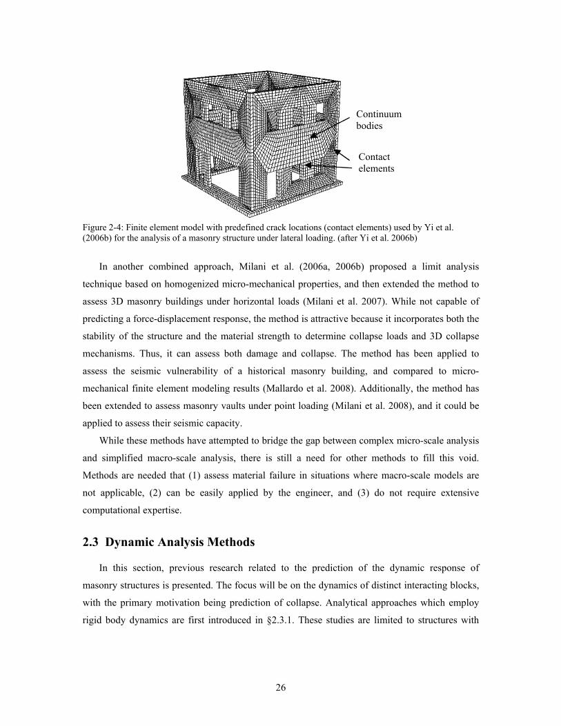
Between these two extremes, Yi et al. (2006b) applied a macro-scale interface method, where

the masonry is modeled as an elastic continuum with contact elements at predefined crack

locations (Figure 2-4). The strength of the material is only assessed at these contact elements. The

authors used shell finite elements to predict the 3D response of a two-story masonry building

under lateral loading. This approach simplifies the analysis considerably, reducing computation

time and convergence problems. It is effective if probable crack locations are known with some

certainty.

(a) (b)

26

Figure 2-4: Finite element model with predefined crack locations (contact elements) used by Yi et al. (2006b) for the analysis of a masonry structure under lateral loading. (after Yi et al. 2006b)

In another combined approach, Milani et al. (2006a, 2006b) proposed a limit analysis

technique based on homogenized micro-mechanical properties, and then extended the method to

assess 3D masonry buildings under horizontal loads (Milani et al. 2007). While not capable of

predicting a force-displacement response, the method is attractive because it incorporates both the

stability of the structure and the material strength to determine collapse loads and 3D collapse

mechanisms. Thus, it can assess both damage and collapse. The method has been applied to

assess the seismic vulnerability of a historical masonry building, and compared to micro-

mechanical finite element modeling results (Mallardo et al. 2008). Additionally, the method has

been extended to assess masonry vaults under point loading (Milani et al. 2008), and it could be

applied to assess their seismic capacity.

While these methods have attempted to bridge the gap between complex micro-scale analysis

and simplified macro-scale analysis, there is still a need for other methods to fill this void.

Methods are needed that (1) assess material failure in situations where macro-scale models are

not applicable, (2) can be easily applied by the engineer, and (3) do not require extensive

computational expertise.

2.3 Dynamic Analysis Methods

In this section, previous research related to the prediction of the dynamic response of

masonry structures is presented. The focus will be on the dynamics of distinct interacting blocks,

with the primary motivation being prediction of collapse. Analytical approaches which employ

rigid body dynamics are first introduced in §2.3.1. These studies are limited to structures with

Continuum bodies

Contact elements

27

relatively few degrees of freedom, motivating the use of discrete body computational methods

which are discussed in §2.3.2.

Continuum methods are often used to assess the dynamics of masonry structures, but they are

beyond the scope of this dissertation. However, it must be mentioned that continuum methods are

typically applied to determine the steady-state dynamic response through modal analysis. The

modal response of the structure is often used to determine where stresses are highest and where

cracking might occur. Thus, continuum methods can be effective in predicting locations of

damage, but fall short when trying to predict collapse or the actual transient dynamic response of

interacting distinct bodies. FEM tools that both incorporate dynamic resonance effects, and

predict dynamic failure once cracking begins, still need to be developed.

2.3.1 Analytical Methods

Several studies have addressed the dynamic response of masonry structures through

derivation of analytical equations of motion. The majority of these studies focus on the most basic

rocking structure, the rocking block, but some address more complex structures like arches and

portal frames.

The Rocking Block

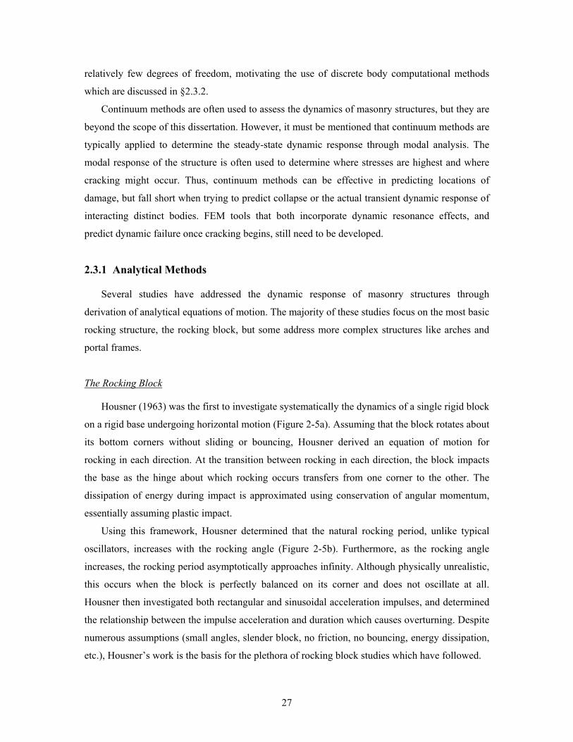
Housner (1963) was the first to investigate systematically the dynamics of a single rigid block

on a rigid base undergoing horizontal motion (Figure 2-5a). Assuming that the block rotates about

its bottom corners without sliding or bouncing, Housner derived an equation of motion for

rocking in each direction. At the transition between rocking in each direction, the block impacts

the base as the hinge about which rocking occurs transfers from one corner to the other. The

dissipation of energy during impact is approximated using conservation of angular momentum,

essentially assuming plastic impact.

Using this framework, Housner determined that the natural rocking period, unlike typical

oscillators, increases with the rocking angle (Figure 2-5b). Furthermore, as the rocking angle

increases, the rocking period asymptotically approaches infinity. Although physically unrealistic,

this occurs when the block is perfectly balanced on its corner and does not oscillate at all.

Housner then investigated both rectangular and sinusoidal acceleration impulses, and determined

the relationship between the impulse acceleration and duration which causes overturning. Despite

numerous assumptions (small angles, slender block, no friction, no bouncing, energy dissipation,

etc.), Housner’s work is the basis for the plethora of rocking block studies which have followed.

28

Figure 2-5: Rocking block analysis by Housner (1963): (a) definition of the rocking motion, and (b) the natural rocking period (T) as a function of the rocking angle θo. (after Housner 1963) Note: Io is the moment of inertia of the block about point O.

Yim et al. (1980) approached the rocking block problem without making small angle

assumptions. Instead, using a fourth order Runge-Kutta integration scheme, the non-linear

equations of motion were solved numerically. Using this numerical solution procedure and

simulated random earthquake ground motions, Yim et al. (1980) addressed the problem of the

magnitude of the simulated earthquake necessary to cause overturning of a rigid block. Due to the

random nature of the loading, the rigid block response was found to vary drastically from

relatively little motion to complete overturning when subjected to the same magnitude of

randomly generated horizontal ground motion. Due to this variability, the problem becomes one

of probability. By repeating simulations for each of several block geometries and ground motion

magnitudes, cumulative probability density functions were plotted. The probability of overturning

was found to increase with an increase in slenderness ratio and magnitude of ground motion, and

decrease with an increase in scale. Small variations (5%) in the restitution coefficient developed

by Housner were found to have a negligible effect on the probability of overturning.

The study by Yim et al. (1980) demonstrates the difficulty in predicting the stability of a

block structure when the ground acceleration (simulated earthquake motion) is randomly

generated, even if the maximum magnitude of the ground acceleration is specified. However,

even though the stability of a structure could not be definitively determined, clear trends were

found which could be used to determine the probability of overturning. In the process, the

(a) (b)

29

uncertainty involved in predicting the rocking response to earthquake motion is clearly

demonstrated, and must be kept in perspective.

While Yim et al. (1980) focused on the rocking block response to randomly generated

earthquake motion, Spanos and Koh (1984) focused on the rocking block response to harmonic

horizontal ground acceleration. Using both the linearized and non-linear equations of motion, the

stability of a rocking block subjected to harmonic ground accelerations of varying frequency and

amplitude was determined. The frequencies and amplitudes for which the steady state modes of

oscillation are stable were also determined. However, these steady state modes are dependent on

perfectly harmonic ground motions. Yim et al. (1980) showed that a slight variation in ground

motion can have a drastic effect on the rocking response. Thus, it seems unlikely that these

steady-state rocking modes could be physically realized.

Following the work by Spanos and Koh (1984), numerous researchers focused on the

response of rocking blocks to harmonic ground motion (e.g., Tso and Wong 1989, Hogan 1990,

Yim and Lin 1991, Shenton and Jones 1991b, Lenci and Rega 2006). Although the rocking

response to harmonic shaking is an interesting dynamical problem, the attention it garnered

perhaps demonstrates a structural dynamics mindset rooted in the concept of the response spectra,

inheriting the assumption that harmonic ground motion could illicit a resonant response.

In addition to investigating different ground motions, researchers have explored more

complex block behaviors including coupled sliding, bouncing, and rocking behavior (e.g. Shenton

and Jones 1991a, Augusti and Sinopoli 1992, Lipscombe 1993, Scalia and Sumbatyan 1996,

Shenton 1996, Pompei et al. 1998). Including these coupled behaviors is important for short, stout

blocks, but is less important for tall, slender blocks.

In contrast to these studies, Zhang and Makris (2001) applied Housner’s original framework

and expanded Housner’s investigation of the rocking response to ground pulses, clearly defining

two distinct failure modes and the corresponding failure domains for cycloidal pulses. Zhang and

Makris (2001) focused their attention on the largest cycloidal impulses within an expected

earthquake ground motion, reasoning that the rotational inertia generated by these impulses are

the driving force of collapse rather than the harmonic response to the frequency spectra. Makris

and Konstantinidis (2003) then critically evaluated the work of Priestley et al. (1978) and

concluded that a rocking structure cannot be replaced by an equivalent ‘typical elastic’ oscillator

and should not be evaluated using response spectra. Makris and Konstantinidis (2003) also

highlighted fundamental differences between rocking blocks and typical elastic oscillators and

proposed the rocking spectra as a unique measure of earthquake intensity.

30

Finally, several researchers have investigated the response of multiple block systems. For

example, in an attempt to bridge the gap between single block rocking and actual masonry

structures, Sinopoli and Sepe (1993) investigated the behavior of a three block frame structure

subjected to horizontal ground acceleration. Similarly, Spanos et al. (2001) analyzed the

dynamics of a stacked two-block structure. The derivation of the equations of motion becomes

quite extensive for this two-block problem, and extending the derivation to several block systems

would be intensive. The authors note that "this effort could perhaps be expedited by incorporating

in the analysis concepts of the discrete elements technique" (Spanos et al. 2001), which will be

discussed in §2.3.2.

The Arch

After studying the response of the arch to a constant horizontal acceleration, both Oppenheim

(1992) and Clemente (1998) extended their quasi-static analyses to dynamic horizontal

acceleration loading. Both authors used their quasi-static analysis to determine hinge locations

and assumed that the resulting SDOF mechanism remains unchanged throughout dynamic

motion. The simplification of this multiple block system to a SDOF equation of motion allows an

analytical solution. Both authors applied a rectangular acceleration impulse and came to the

expected conclusion that the allowable ground acceleration is highly dependent on both the

duration and magnitude of the ground acceleration. The arch was found to remain standing under

large ground accelerations of short durations, and as the impulse duration increases, the allowable

horizontal acceleration asymptotically decreases to the quasi-static allowable horizontal

acceleration. In their analyses, both authors only considered the first half-cycle of oscillation, i.e.

until the arch first returns to the natural configuration.

The equations of motion derived by both authors are independent of the mass (or density) of

the blocks, but are dependent on the overall scale of the structure. Oppenheim (1992) noted that

the acceleration impulse necessary to cause collapse approximately increased by the square root

of the arch radius. In other words, larger structures are more resistant to base accelerations than

smaller ones.

Although neither Oppenheim (1992) nor Clemente (1998) verified their modeling

experimentally, Appleton (1999) conducted an experimental investigation inspired by the work of

Oppenheim. She constructed arches and tilted them to verify her quasi-static numerical analysis,

and also tested arches under a variety of horizontal ground motions.

31

2.3.2 Computational Methods

Although analytical solutions provide insight regarding the nature of the dynamics of

masonry structures, their complexity demonstrates the need for computational tools which can

correctly address the problem of rigid block dynamics. Initially, finite element programs were the

computational tools of choice for most engineers, but they are optimal for problems of elasticity

and plasticity, not stability. The more recent application of Discrete Element Modeling (DEM)

inherently captures the discontinuous nature of masonry.

Several different techniques for modeling the dynamic interaction of discrete blocks have

been taken, all of which allow complete separation of blocks and can recognize new contacts as

blocks impact each other. The way that these methods address contact between blocks can be

divided into two primary categories. The first category involves methods which allow slight block

interpenetration, referred to as “compliant contact.” These methods employ a spring-dashpot

element where contact is recognized. The Universal Distinct Element Code (UDEC) and the 3-

dimesional Distinct Element Code (3DEC), both distributed commercially by Itasca

(www.itascacg.com), fall into this category and will be discussed. The second category includes

methods in which zero block interpenetration is allowed, referred to as “unilateral contact.” These

methods rigorously prevent block overlap by aligning block boundaries where contact is

recognized. Non-Smooth Contact Dynamics (NSCD) falls into this category and will also be

discussed.

UDEC / 3DEC

UDEC (Itasca 2004) and 3DEC (Itasca 2003) are probably the most widely applied discrete

methods, and are both based on the research of Cundall (1971, 1980) and Cundall and Strack

(1979). Explicit integration is used with sufficiently small time steps to ensure computational

stability. Blocks can be either rigid or deformable, and joint properties and Rayleigh damping

properties must be defined. Details of these programs are discussed further in Chapter 7.

UDEC has been applied to model the response of several masonry structures to ground

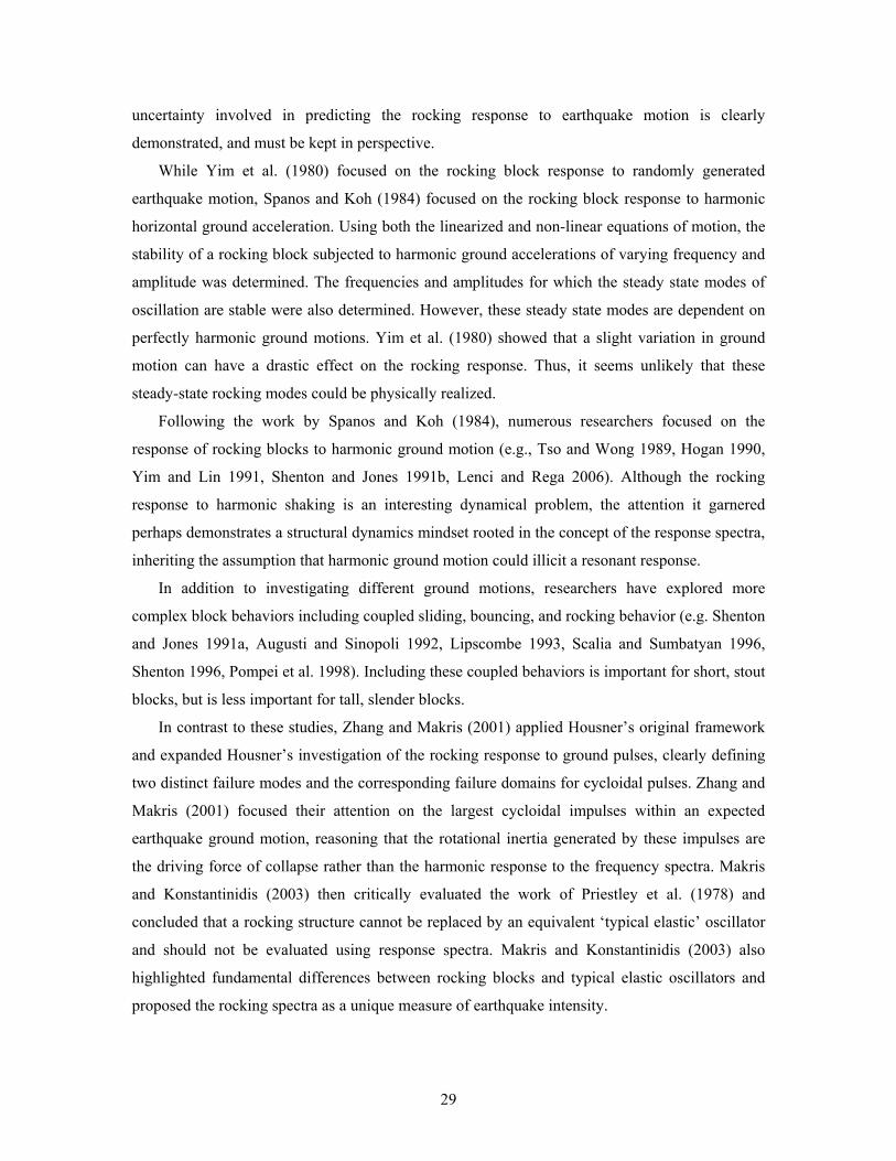
motion (e.g. Azevedo et al. 2000, Psycharis et al. 2000, Drei and Fontana 2003). While these

studies show the potential of the method to predict the collapse of masonry structures (Figure 2-

6), there is little mention of modeling parameters or assumptions, and the results are not verified.

32

Figure 2-6: Seismic behavior and collapse patterns for two different masonry structures under seismic loading. (after Azevedo et al. 2000)

UDEC also has been used to evaluate the response of rocking blocks, and two studies in

particular propose methods for defining joint and stiffness properties and compare results with

experimental tests. First, Winkler et al. (1995) applied the discrete element method to simulate

the response of one, two, and three stacked blocks, in an attempt to evaluate furniture overturning

in an earthquake. They defined joint stiffness properties based on measured material properties of

the blocks that they tested, and defined damping properties by fitting UDEC predictions to match

free-rocking experiments. They focused on harmonic base motion, and found good agreement

between numerical and experimental results. Second, Peña et al. (2007) used UDEC to predict the

response of a single rocking block to both harmonic and earthquake ground motions. Instead of

defining joint properties according to the material of the blocks tested, joint properties were

defined based on an analytically derived frequency parameter of the system. Once joint properties

were defined, stiffness-proportional damping properties were derived to approximate the

analytical damping employed by Housner’s restitution coefficient. Subsequently, the modeling

parameters were improved by fitting them to free-rocking experimental results. The method

resulted in an unrealistically soft joint interface, from which the block does not separate during

rocking motion. Thus, continual damping is applied in order to approximate actual damping

which primarily occurs at impact. After fitting, the method was effective in predicting

experimental results of more complex ground motions.

33

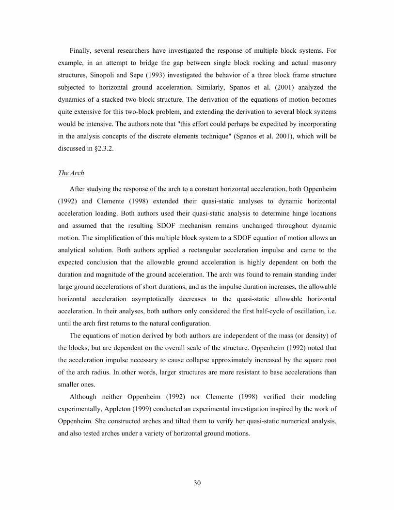
Figure 2-7: Collapse mechanisms formed by intersecting masonry arches under horizontal ground motion. (after Lemos 1998)

The response of masonry structures to ground motion has also been investigated using 3DEC.

Lemos (1998) assessed the three-dimensional stability of masonry arches due to ground motion,

and predicted interesting collapse mechanisms (Figure 2-7). More recently, Lemos (2007)

critically evaluated numerical issues which can arise when trying to model structural dynamics

using discrete elements, and mentions some difficulties involved in defining damping.

Papantonopoulos et al. (2002) simulated experiments on a one-third scale replica of a Parthenon

column conducted by Mouzakis et al. (2002). The authors did a sensitivity study to determine

appropriate damping parameters, and concluded that 3DEC can be used with confidence to

estimate the response of ancient monuments to expected earthquake motions. Subsequently,

Psycharis et al. (2003) used 3DEC to assess the stability of the entire Parthenon Pronaos.

While many of these studies conclude that UDEC and 3DEC are effective in predicting

results, this can only be concluded after modeling parameters are adjusted so that results do

compare well. A methodical way of defining modeling parameters before analysis is still lacking.

This is necessary before confidence can be placed in DEM prediction.

NSCD

Non-smooth contact dynamics involves an implicit time-stepping scheme in which blocks can

be either rigid or deformable. Unilateral contact is based on the work of Moreau (1988), and

ensures that blocks do not interpenetrate and contacting bodies do not attract each other, i.e.

normal contact forces remain outward. Coulomb friction is included in the model. The impact

between rigid blocks is taken into account using shock laws, in which the energy dissipation can

theoretically be adjusted by the “dissipation index” (Moreau 1988). The NSCD method was

formalized by Jean (1998), in which standard inelastic shock (Moreau 1984) is assumed.

34

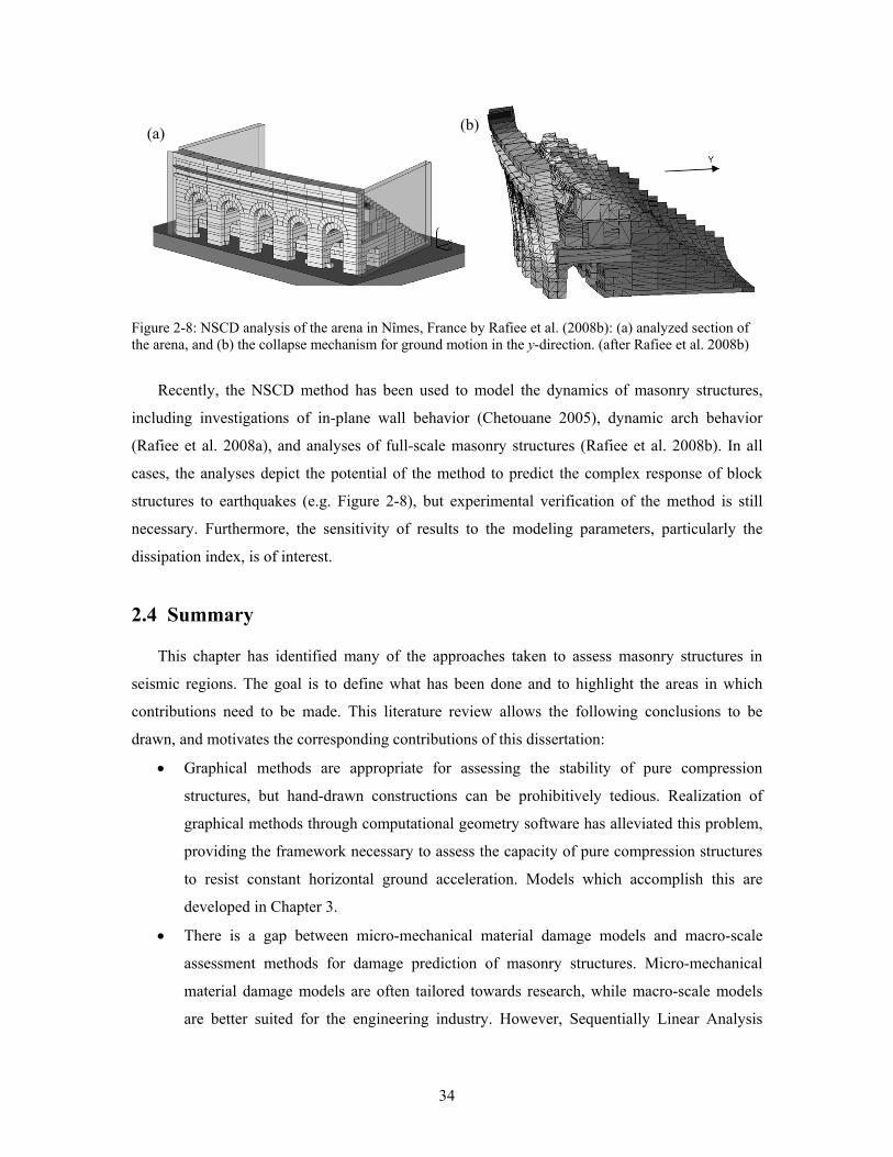
Figure 2-8: NSCD analysis of the arena in Nîmes, France by Rafiee et al. (2008b): (a) analyzed section of the arena, and (b) the collapse mechanism for ground motion in the y-direction. (after Rafiee et al. 2008b)

Recently, the NSCD method has been used to model the dynamics of masonry structures,

including investigations of in-plane wall behavior (Chetouane 2005), dynamic arch behavior

(Rafiee et al. 2008a), and analyses of full-scale masonry structures (Rafiee et al. 2008b). In all

cases, the analyses depict the potential of the method to predict the complex response of block

structures to earthquakes (e.g. Figure 2-8), but experimental verification of the method is still

necessary. Furthermore, the sensitivity of results to the modeling parameters, particularly the

dissipation index, is of interest.

2.4 Summary

This chapter has identified many of the approaches taken to assess masonry structures in

seismic regions. The goal is to define what has been done and to highlight the areas in which

contributions need to be made. This literature review allows the following conclusions to be

drawn, and motivates the corresponding contributions of this dissertation:

• Graphical methods are appropriate for assessing the stability of pure compression

structures, but hand-drawn constructions can be prohibitively tedious. Realization of

graphical methods through computational geometry software has alleviated this problem,

providing the framework necessary to assess the capacity of pure compression structures

to resist constant horizontal ground acceleration. Models which accomplish this are

developed in Chapter 3.

• There is a gap between micro-mechanical material damage models and macro-scale

assessment methods for damage prediction of masonry structures. Micro-mechanical

material damage models are often tailored towards research, while macro-scale models

are better suited for the engineering industry. However, Sequentially Linear Analysis

(a) (b) (a)

35

(SLA) has been proposed as a simplified alternative to model damage of masonry

structures which could bridge this gap (Rots 2001). This method is discussed, further

developed, and applied in Chapter 4.

• While rigid body dynamics is a powerful method for analytically determining the

response of rigid block structures, it becomes cumbersome for multiple block systems

and is therefore reaching its practical limits. However, the simplification of arches as

SDOF mechanisms holds potential for describing the dynamics of arches using analytical

rigid body dynamics. Furthermore, the dynamics of arches has not been thoroughly

explored experimentally. An analytical arch model is developed and compared with new

experimental results in Chapter 5.

• While rocking behavior has been extensively studied, a clear investigation into the

ground motions to which rocking structures are most vulnerable has not been conducted.

Furthermore, while research suggests that the primary impulse within an earthquake

excitation is the critical factor which causes overturning of rocking structures, the

possibility that multiple impulses could act together to amplify the rocking response has

not been addressed. These concepts are explored in Chapter 6.

• Discrete element models with compliant contacts (e.g. UDEC) have been effective in

capturing the general dynamic behavior of masonry structures to earthquake ground

motions. However, further evaluation of these methods is necessary, and a clearer

understanding of modeling limitations should encourage intelligent ways in which these

methods can be confidently applied. Additionally, a systematic way of defining modeling

parameters is lacking. These challenges are addressed in Chapter 7.

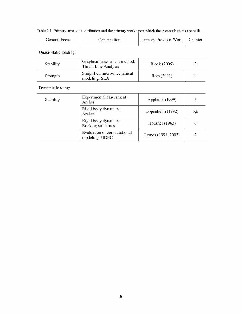
The areas in which the contributions of this dissertation are made are summarized in Table

2.1, where the primary research studies upon which contributions are built are also cited.

36

Table 2.1: Primary areas of contribution and the primary work upon which these contributions are built

General Focus Contribution Primary Previous Work Chapter

Quasi-Static loading:

Stability Graphical assessment method: Thrust Line Analysis Block (2005) 3

Strength Simplified micro-mechanical modeling: SLA Rots (2001) 4

Dynamic loading:

Stability Experimental assessment: Arches Appleton (1999) 5

Rigid body dynamics: Arches Oppenheim (1992) 5,6

Rigid body dynamics: Rocking structures Housner (1963) 6

Evaluation of computational modeling: UDEC Lemos (1998, 2007) 7

37

Part II

Quasi-static Analysis

38

Chapter 3

Thrust Line Analysis

3.1 Introduction

For assessing masonry structures in seismic regions, it is necessary to understand quasi-static

collapse before moving on to dynamic collapse. This chapter focuses on a quasi-static assessment

method based purely on stability. Once stability limits are determined, then assessment methods

based on strength can be applied to model damage if desired, as in Chapter 4.

As discussed in §2.2.1, equilibrium methods are effective for the assessment of masonry

under static loading (Heyman 1995). Under the assumptions of these methods, sliding and

crushing are not possible, but stability can be assessed. The concept of a thrust line is used to

visualize the forces within the structure. When the thrust line can no longer be contained within

the masonry, the masonry can no longer support the applied loads, and the structure is no longer

in equilibrium without hinging. In general, hinging does not necessarily mean that the collapse of

the structure is eminent, because four hinges are necessary to form an unstable mechanism. Take

for example, the arch on spreading supports. Three hinges form immediately under an applied

support displacement, but the thrust line remains within the masonry and the structure therefore

remains stable until four hinges form at the point of collapse (Ochsendorf 2006). On the other

hand, applied forces do not cause any hinging until a four-hinge mechanism directly forms.

Although the static analysis of arched structures has been studied for centuries, Block (2005)

recently developed a tool which uses graphic statics to achieve a rapid first order assessment of

39

the stability of various masonry structures. A parametric graphical framework allows geometry to

be adjusted in real-time, allowing the effect of geometrical changes to be rapidly evaluated. All

graphical constructions presented in this chapter were implemented using Cabri Geometry II Plus

(www.cabri.com), a commercial geometric modeling software. For a review of graphic statics,

see Zalewski and Allen (1998).

3.2 Tilt Analysis

As mentioned in Chapter 2, it is common practice in structural engineering design to simulate

earthquake loading by a constant horizontal force that is some fraction of the weight of the

structure in magnitude. This is equivalent to applying a constant horizontal acceleration that is

some fraction of the acceleration of gravity. Such an ‘equivalent static loading’ does not capture

all of the dynamics, but it does provide a measure of the lateral loading that the structure could

withstand before collapse.

One way of implementing equivalent static analysis is by tilting the ground surface. This

effectively applies a combination of vertical and horizontal acceleration to the structure. Note that

in the reference frame that rotates with the structure, tilting causes the vertical acceleration to be

reduced as horizontal acceleration increases. Thus, tilting is not exactly the same as only applying

constant horizontal ground acceleration. However, while this would be problematic if the stresses

within the structure were of interest, the assumption that crushing will not occur negates this

problem. The ratio of vertical to horizontal acceleration is all that is of interest, and the fact that

stresses within the structure are effectively reduced is assumed to be of secondary importance.

The ratio of horizontal acceleration ( hu ) to vertical acceleration ( vu ) in the rotating reference

frame is directly related to the angle of tilt (α):

tan= =h

v

uu

γ α (3.1)

In this chapter, graphic statics is used to develop a tool to simulate structures on a tilting

surface. The ground surface is tilted until the thrust line cannot be contained within the structure,

i.e. until the point where it touches the exterior surface of the structure at four locations. At this

point, a four-hinge mechanism would form and the structure would collapse.

Although it is trivial, the overturning collapse of a single block helps to clarify tilting thrust

line analysis. The single block in Figure 3-1a is only acted upon by gravity, and therefore the

thrust line is drawn vertically downward from the center of mass. In this initial state, the thrust

line remains within the block until it enters the supporting ground, thus the block is stable. If the

40

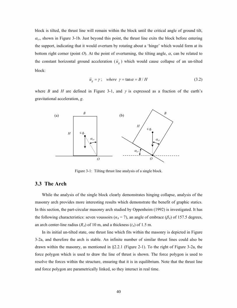
block is tilted, the thrust line will remain within the block until the critical angle of ground tilt,

αcr, shown in Figure 3-1b. Just beyond this point, the thrust line exits the block before entering

the support, indicating that it would overturn by rotating about a ‘hinge’ which would form at its

bottom right corner (point O). At the point of overturning, the tilting angle, α, can be related to

the constant horizontal ground acceleration ( gu ) which would cause collapse of an un-tilted

block:

; tan /= = =gu where B Hγ γ α (3.2)

where B and H are defined in Figure 3-1, and γ is expressed as a fraction of the earth’s

gravitational acceleration, g.

Figure 3-1: Tilting thrust line analysis of a single block.

3.3 The Arch

While the analysis of the single block clearly demonstrates hinging collapse, analysis of the

masonry arch provides more interesting results which demonstrate the benefit of graphic statics.

In this section, the part-circular masonry arch studied by Oppenheim (1992) is investigated. It has

the following characteristics: seven voussoirs (nA = 7), an angle of embrace (βA) of 157.5 degrees,

an arch center-line radius (RA) of 10 m, and a thickness (tA) of 1.5 m.

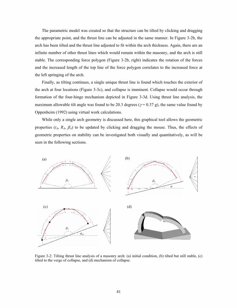
In its initial un-tilted state, one thrust line which fits within the masonry is depicted in Figure

3-2a, and therefore the arch is stable. An infinite number of similar thrust lines could also be

drawn within the masonry, as mentioned in §2.2.1 (Figure 2-1). To the right of Figure 3-2a, the

force polygon which is used to draw the line of thrust is shown. The force polygon is used to

resolve the forces within the structure, ensuring that it is in equilibrium. Note that the thrust line

and force polygon are parametrically linked, so they interact in real time.

B

H αcr

c.g.

O

B

H

αcr

c.g.

O

αcr

(a) (b)

41

The parametric model was created so that the structure can be tilted by clicking and dragging

the appropriate point, and the thrust line can be adjusted in the same manner. In Figure 3-2b, the

arch has been tilted and the thrust line adjusted to fit within the arch thickness. Again, there are an

infinite number of other thrust lines which would remain within the masonry, and the arch is still

stable. The corresponding force polygon (Figure 3-2b, right) indicates the rotation of the forces

and the increased length of the top line of the force polygon correlates to the increased force at

the left springing of the arch.

Finally, as tilting continues, a single unique thrust line is found which touches the exterior of

the arch at four locations (Figure 3-3c), and collapse is imminent. Collapse would occur through

formation of the four-hinge mechanism depicted in Figure 3-3d. Using thrust line analysis, the

maximum allowable tilt angle was found to be 20.3 degrees (γ = 0.37 g), the same value found by

Oppenheim (1992) using virtual work calculations.

While only a single arch geometry is discussed here, this graphical tool allows the geometric

properties (tA, RA, βA) to be updated by clicking and dragging the mouse. Thus, the effects of

geometric properties on stability can be investigated both visually and quantitatively, as will be

seen in the following sections.

Figure 3-2: Tilting thrust line analysis of a masonry arch: (a) initial condition, (b) tilted but still stable, (c) tilted to the verge of collapse, and (d) mechanism of collapse.

αcr

βA

βA

α

(a) (b)

(d) (c)

βA

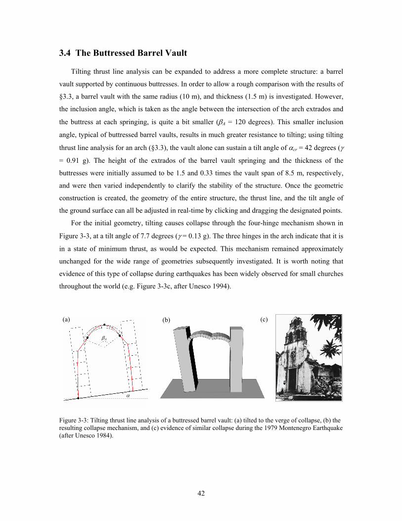
42

3.4 The Buttressed Barrel Vault

Tilting thrust line analysis can be expanded to address a more complete structure: a barrel

vault supported by continuous buttresses. In order to allow a rough comparison with the results of

§3.3, a barrel vault with the same radius (10 m), and thickness (1.5 m) is investigated. However,

the inclusion angle, which is taken as the angle between the intersection of the arch extrados and

the buttress at each springing, is quite a bit smaller (βA = 120 degrees). This smaller inclusion

angle, typical of buttressed barrel vaults, results in much greater resistance to tilting; using tilting

thrust line analysis for an arch (§3.3), the vault alone can sustain a tilt angle of αcr = 42 degrees (γ

= 0.91 g). The height of the extrados of the barrel vault springing and the thickness of the

buttresses were initially assumed to be 1.5 and 0.33 times the vault span of 8.5 m, respectively,

and were then varied independently to clarify the stability of the structure. Once the geometric

construction is created, the geometry of the entire structure, the thrust line, and the tilt angle of

the ground surface can all be adjusted in real-time by clicking and dragging the designated points.

For the initial geometry, tilting causes collapse through the four-hinge mechanism shown in

Figure 3-3, at a tilt angle of 7.7 degrees (γ = 0.13 g). The three hinges in the arch indicate that it is

in a state of minimum thrust, as would be expected. This mechanism remained approximately

unchanged for the wide range of geometries subsequently investigated. It is worth noting that

evidence of this type of collapse during earthquakes has been widely observed for small churches

throughout the world (e.g. Figure 3-3c, after Unesco 1994).

Figure 3-3: Tilting thrust line analysis of a buttressed barrel vault: (a) tilted to the verge of collapse, (b) the resulting collapse mechanism, and (c) evidence of similar collapse during the 1979 Montenegro Earthquake (after Unesco 1984).

βA

α

(a) (b) (c)

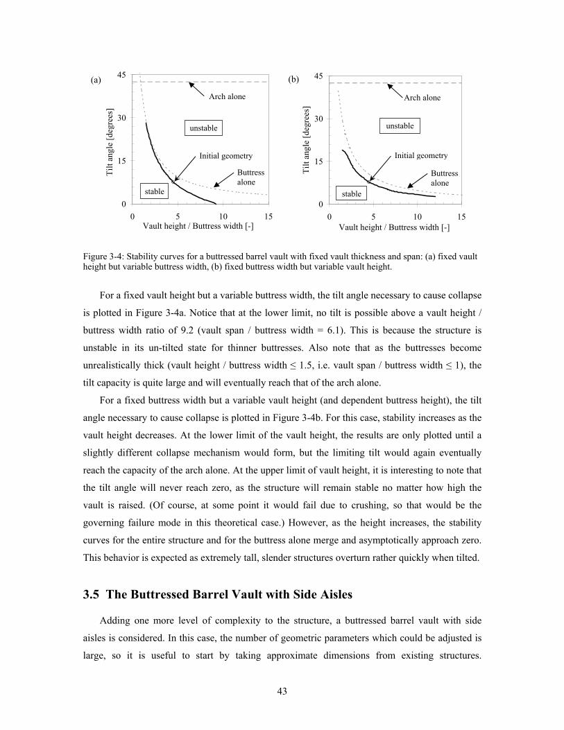
43

Figure 3-4: Stability curves for a buttressed barrel vault with fixed vault thickness and span: (a) fixed vault height but variable buttress width, (b) fixed buttress width but variable vault height.

For a fixed vault height but a variable buttress width, the tilt angle necessary to cause collapse

is plotted in Figure 3-4a. Notice that at the lower limit, no tilt is possible above a vault height /

buttress width ratio of 9.2 (vault span / buttress width = 6.1). This is because the structure is

unstable in its un-tilted state for thinner buttresses. Also note that as the buttresses become

unrealistically thick (vault height / buttress width ≤ 1.5, i.e. vault span / buttress width ≤ 1), the

tilt capacity is quite large and will eventually reach that of the arch alone.

For a fixed buttress width but a variable vault height (and dependent buttress height), the tilt

angle necessary to cause collapse is plotted in Figure 3-4b. For this case, stability increases as the

vault height decreases. At the lower limit of the vault height, the results are only plotted until a

slightly different collapse mechanism would form, but the limiting tilt would again eventually

reach the capacity of the arch alone. At the upper limit of vault height, it is interesting to note that

the tilt angle will never reach zero, as the structure will remain stable no matter how high the

vault is raised. (Of course, at some point it would fail due to crushing, so that would be the

governing failure mode in this theoretical case.) However, as the height increases, the stability

curves for the entire structure and for the buttress alone merge and asymptotically approach zero.

This behavior is expected as extremely tall, slender structures overturn rather quickly when tilted.

3.5 The Buttressed Barrel Vault with Side Aisles

Adding one more level of complexity to the structure, a buttressed barrel vault with side

aisles is considered. In this case, the number of geometric parameters which could be adjusted is

large, so it is useful to start by taking approximate dimensions from existing structures.

0

15

30

45

0 5 10 15Vault height / Buttress width [-]

Tilt

angl

e [d

egre

es]

(a) (b)

unstable

stablestable

Arch alone

Buttress alone

unstable

Arch alone

0

15

30

45

0 5 10 15Vault height / Buttress width [-]

Tilt

angl

e [d

egre

es]

Initial geometry

Buttress alone

Initial geometry

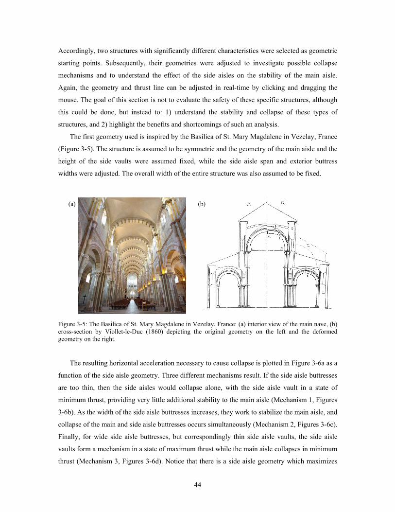
44

Accordingly, two structures with significantly different characteristics were selected as geometric

starting points. Subsequently, their geometries were adjusted to investigate possible collapse

mechanisms and to understand the effect of the side aisles on the stability of the main aisle.

Again, the geometry and thrust line can be adjusted in real-time by clicking and dragging the

mouse. The goal of this section is not to evaluate the safety of these specific structures, although

this could be done, but instead to: 1) understand the stability and collapse of these types of

structures, and 2) highlight the benefits and shortcomings of such an analysis.

The first geometry used is inspired by the Basilica of St. Mary Magdalene in Vezelay, France

(Figure 3-5). The structure is assumed to be symmetric and the geometry of the main aisle and the

height of the side vaults were assumed fixed, while the side aisle span and exterior buttress

widths were adjusted. The overall width of the entire structure was also assumed to be fixed.

Figure 3-5: The Basilica of St. Mary Magdalene in Vezelay, France: (a) interior view of the main nave, (b) cross-section by Viollet-le-Duc (1860) depicting the original geometry on the left and the deformed geometry on the right.

The resulting horizontal acceleration necessary to cause collapse is plotted in Figure 3-6a as a

function of the side aisle geometry. Three different mechanisms result. If the side aisle buttresses

are too thin, then the side aisles would collapse alone, with the side aisle vault in a state of

minimum thrust, providing very little additional stability to the main aisle (Mechanism 1, Figures

3-6b). As the width of the side aisle buttresses increases, they work to stabilize the main aisle, and

collapse of the main and side aisle buttresses occurs simultaneously (Mechanism 2, Figures 3-6c).

Finally, for wide side aisle buttresses, but correspondingly thin side aisle vaults, the side aisle

vaults form a mechanism in a state of maximum thrust while the main aisle collapses in minimum

thrust (Mechanism 3, Figures 3-6d). Notice that there is a side aisle geometry which maximizes

(a) (b)

45

the tilt angle which can be achieved (Figure 3-6a), and therefore optimizes the relationship

between the side aisle span and the buttress width.

Compared to the range of buttressed barrel vaults investigated in §3.5, the main aisle alone is

not very stable (Figure 3-6a). This is expected as the side aisles are intended to support the main

aisle. In this rough approximation, the side aisles approximately double the angle of tilt that the

structure could withstand. It is worth noting that the side aisles are short with respect to the height

of the main aisle, which limits their effectiveness in providing additional stability. While the

cause of the deformations depicted by Viollet-le-Duc (1860) on the right of Figure 3-5b is

unknown, the solution was to add flying buttresses on both sides of the main aisle (drawn dashed

above the right side aisle in Figure 3-5b). This solution solves the problem of the limited

stabilizing capacity of the short side aisles.

The second geometry used is inspired by the Church of Saint Patrocle in Colombier, France

(Figure 3-7a). In this structure, the side aisles are almost as tall as the main aisle, and much taller

than in the basilica in Vezelay. Taking an approximation of a cross-section of the church in

Colombier from the database of Bourbonnais churches compiled at Columbia University (Murray

2009), the effect of the side-aisles on stability is again investigated using the same geometric

assumptions made for Vezelay. Initially, the exterior buttresses, which were added to one side of

the church well after construction (Figure 3-8a), are ignored. Subsequently, the effect of these

buttresses on the stability is briefly evaluated.

The resulting horizontal acceleration at collapse is again plotted as a function of side aisle

geometry in Figure 3-7b. Three primary collapse mechanisms result (Figure 3-7), which differ

from those in Figure 3-6 due to the taller side aisles. For thin side aisle buttresses, the side aisles

again collapse alone before the main aisle (Mechanism 1, Figure 3-7c), and again provide very

little additional stability. For wider side aisle buttresses, the stability increases significantly. The

higher side aisles cause all three vaults to collapse in unison, with the right side aisle in minimum

thrust and the other two at intermediate states of thrust (Mechanism 2b, Figure 3-7d). This is

noticeably different than the case of Vezelay, in which the right side aisle is never predicted to

collapse. Last, as the side aisle buttresses get extremely wide, the side aisle arches again become

the weak link. All three vaults collapse together, with the left, center and right vaults being in

maximum, intermediate, and minimum states of thrust, respectively (Mechanism 3b, Figure 3-7e).

Again notice that there is an optimal side aisle geometry which maximizes the stability of the

entire system, and provides roughly three times the tilt capacity of the main aisle alone (Figure 3-

7b). However, this would require side aisle buttresses which are extremely thick, inspiring the

alternate solution of the flying buttress.

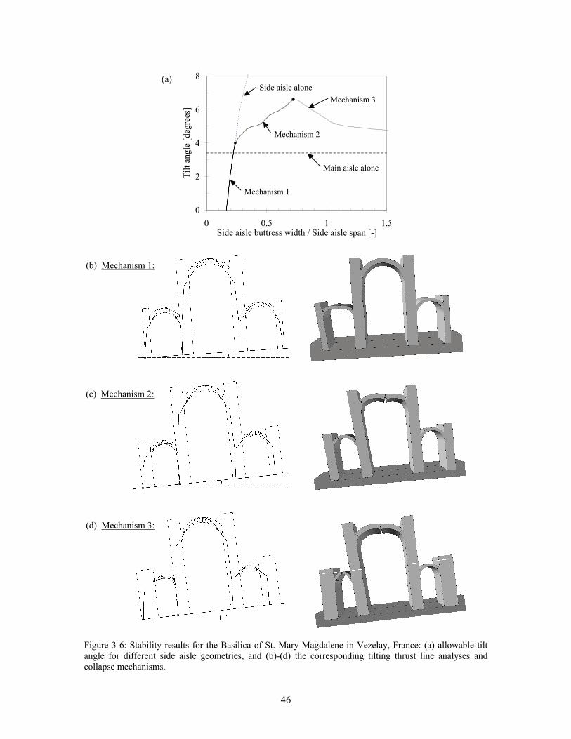
46

Figure 3-6: Stability results for the Basilica of St. Mary Magdalene in Vezelay, France: (a) allowable tilt angle for different side aisle geometries, and (b)-(d) the corresponding tilting thrust line analyses and collapse mechanisms.

0

2

4

6

8

0 0.5 1 1.5Side aisle buttress width / Side aisle span [-]

Tilt

angl

e [d

egre

es]

(b) Mechanism 1:

(d) Mechanism 3:

(c) Mechanism 2:

(a)

Main aisle alone

Side aisle alone

Mechanism 1

Mechanism 2

Mechanism 3

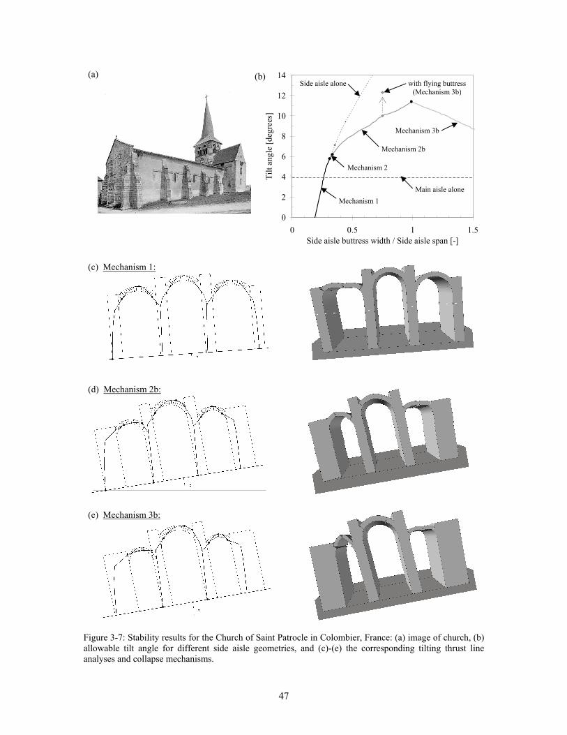
47

Figure 3-7: Stability results for the Church of Saint Patrocle in Colombier, France: (a) image of church, (b) allowable tilt angle for different side aisle geometries, and (c)-(e) the corresponding tilting thrust line analyses and collapse mechanisms.

(c) Mechanism 1:

(e) Mechanism 3b:

(d) Mechanism 2b:

0

2

4

6

8

10

12

14

0 0.5 1 1.5Side aisle buttress width / Side aisle span [-]

Tilt

angl

e [d

egre

es]

Main aisle alone

Side aisle alone

Mechanism 1

Mechanism 2b

Mechanism 3b

Mechanism 2

with flying buttress (Mechanism 3b)

(a) (b)

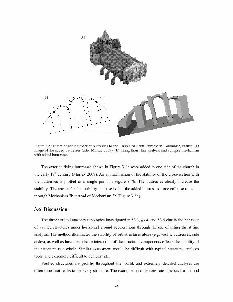
48

Figure 3-8: Effect of adding exterior buttresses to the Church of Saint Patrocle in Colombier, France: (a) image of the added buttresses (after Murray 2009), (b) tilting thrust line analysis and collapse mechanism with added buttresses.

The exterior flying buttresses shown in Figure 3-8a were added to one side of the church in

the early 19th century (Murray 2009). An approximation of the stability of the cross-section with

the buttresses is plotted as a single point in Figure 3-7b. The buttresses clearly increase the

stability. The reason for this stability increase is that the added buttresses force collapse to occur

through Mechanism 3b instead of Mechanism 2b (Figure 3-8b).

3.6 Discussion

The three vaulted masonry typologies investigated in §3.3, §3.4, and §3.5 clarify the behavior

of vaulted structures under horizontal ground accelerations through the use of tilting thrust line

analysis. The method illuminates the stability of sub-structures alone (e.g. vaults, buttresses, side

aisles), as well as how the delicate interaction of the structural components effects the stability of

the structure as a whole. Similar assessment would be difficult with typical structural analysis

tools, and extremely difficult to demonstrate.

Vaulted structures are prolific throughout the world, and extremely detailed analyses are

often times not realistic for every structure. The examples also demonstrate how such a method

(a)

(b)

49

could be used to rapidly assess the seismic capacity of a large number of vaulted structures of a

certain type. Then more extensive analyses could be conducted on the structures which are

determined to be the least safe.

Furthermore, while this chapter has emphasized the use of tilting analysis as a first order

seismic assessment method, the concept is also valuable as a general stability measure of masonry

structures in non-seismic regions. In the worst case, a stable structure can sustain zero tilt,

signifying no factor of safety. On the other hand, a larger tilt capacity indicates increased

stability, and therefore a greater factor of safety.

While this method is both instructional and effective, numerous simplifications have been

made, resulting in the following limitations:

• Tilting analysis is a quasi-static assessment method which predicts the collapse of the

structure under constant horizontal ground acceleration. Thus, the predicted horizontal

accelerations which cause collapse are extremely conservative in that they assume an

infinite duration of loading. Actual earthquake loadings are obviously of much shorter

duration. For finite durations of ground acceleration, the structure could recover due to

inertial effects, even if a mechanism is briefly formed due to horizontal accelerations

above the predicted acceptable level. This is clearly demonstrated and investigated in Part

II of this dissertation. Additionally, other effects of dynamic loading (e.g. impact and

vibration displacements between blocks) are also ignored by a static analysis.

• As mentioned previously, the assumptions of limit analysis remove the possibility of

local crushing and sliding. For the types of structures discussed in this chapter, these

behaviors typically have a negligible effect under static loading (Ochsendorf and De

Lorenzis 2008). However, for certain types of structures, they could cause results to be

unconservative. For these structures, failure is typically captured with methods focused

on strength rather than stability, as demonstrated in Chapter 4.

• The method presented is currently limited to two-dimensional problems. The structure

should be simplified from three-dimensions to two-dimensions in a manner that ensures

that results are conservative.

Despite these limitations, the method is valuable as a starting point for assessing masonry

structures in seismic regions.

50

3.7 Summary

Equilibrium methods have a strong tradition in the analysis of masonry structures, where

stability often governs. This chapter has demonstrated how these methods can be extended to

provide a first order seismic assessment using graphical analysis. The primary conclusions are as

follows:

• Thrust line analysis is particularly advantageous for studying numerous structures with

similar geometry. Once models are constructed for a certain structural typology (as in

§3.3, §3.4, and §3.5) a first order assessment of stability can be rapidly obtained.

Furthermore, effects of changes in geometry can be rapidly evaluated.

• The results obtained are both qualitative and visual, giving the user a clear depiction of

the collapse mechanism and a better understanding of structural behavior.

• The framework of real-time graphic statics is valuable for design, as the user can adjust

the geometry and immediately get feedback on the stability of their structural form.

• The tools developed in this section are also valuable for instructional purposes, where

visual depiction of results is particularly valuable.

Therefore, while more rigorous dynamic analyses should be executed for structures which are

known to be in danger of collapse, this equivalent static analysis method can provide a valuable

tool for identifying those structures which are in danger, as well as likely collapse mechanisms to

be concerned about.

51

Chapter 4

Sequentially Linear Analysis*

4.1 Introduction

At the opposite end of the spectrum from equilibrium assessment methods (e.g. Chapter 3),

lie analysis methods which focus on strength. These methods attempt to predict material

deformations and material failure, but can have difficulty predicting collapse. Equilibrium

methods, on the other hand, can predict collapse but are not capable of predicting material

behavior and material failure. Thus, strength methods are particularly appropriate when

attempting to predict material damage. More generally, they should be used if neglecting material

deformation, tensile capacity, and compressive failure is undesirable or unconservative.

Strength methods are often appropriate when simulating the response of more modern

masonry structures under simplified quasi-static earthquake loading. If these structures have some

appreciable tensile capacity or are tied together with reinforced concrete or timber floor

diaphragms, the likelihood of collapse due to instability is relatively low, and the tensile and

compressive strengths of masonry must be accounted for in the analysis. In these cases, failure

through material damage can not be neglected.

Strength methods might also be appropriate when trying to predict or explain damage in

vaulted or domed structures with complex geometries. For example, consider what happens if a

* This research was conducted at the Technical University of Delft under the supervision of Professors Jan Rots and Max Hendriks.

52

constant horizontal acceleration were applied to a complex vault made of several layers of

mortared thin tile. The collapse mechanism might not be immediately obvious, and might be

difficult to predict using equilibrium methods. However, strength methods could be used to

predict where damage might occur, which could inform possible collapse mechanisms. Then,

equilibrium methods could be used to predict collapse.

As discussed in §2.2.2, the majority of strength methods employ Finite Element Modeling

(FEM), the framework that will be used in this chapter. Modeling the fracture of brittle materials

is an essential requirement for predicting damage to masonry structures, and remains a challenge

using FEM due to sharp material “softening” after realization of the material strength. Nonlinear

finite element analysis techniques have been adapted to deal with the sharp softening curves

associated with brittle materials like masonry, but convergence difficulties still motivate alternate

modeling procedures.

In this chapter, one alternate method for modeling brittle fracture, Sequentially Linear

Analysis (SLA), will be discussed and further developed. The motivation for this is to fill the void

between existing masonry analysis methods which focus on strength, as reviewed in §2.2.2.

Specifically, the goal is to bridge the gap between simplified macro-scale analyses (e.g. linear

elastic analysis, pier-spring models, equivalent frame analysis) typically employed in engineering

practice and advanced non-linear finite element analyses being applied in academic research. To

achieve this, the aim is to model the 3D response of masonry structures under lateral loading,

while avoiding: 1) the discretization of walls into equivalent frames, 2) the a priori definition of

crack locations, and 3) the convergence difficulties which can occur during non-linear finite

element analysis.

In §4.2, SLA is reviewed. In §4.3, the SLA framework is extended to include non-

proportional loading. The accuracy of this extension, which is critical to allow the inclusion of

self-weight in addition to seismic loads, is verified through simulation of previous experiments

involving brittle fracture. In §4.4, the framework is extended to include shell elements, for the

purpose of predicting three dimensional crack patterns and possible failure mechanisms for

masonry structures under seismic loading. Experiments on a full-scale masonry structure under

cyclic quasi-static loading are simulated to exemplify the capabilities and limitations of the

method. Finally, conclusions and findings are summarized in §4.5.

53

4.2 Review of Sequentially Linear Analysis

Modeling fracture through an event-by-event cracking procedure is an attractive alternative to

typical FEM because modeling proceeds by imposing an increment of damage instead of an

increment of displacement, force, or time. In this way, it is unnecessary to make large jumps in

damage during a single load step or time step, which is usually the source of convergence

problems. In other words, while nonlinear finite element analysis “skips over” portions of the

structural response when brittle behavior occurs, and hopefully rejoins the response through

iteration algorithms, event-by-event procedures avoid this by specifying damage directly.

For example, discrete lattice models (e.g. Herrmann et al. 1989, Schlangen 1993), which have

become quite attractive for modeling fracture, impose incremental damage by breaking a single

beam element in every step. Recently, Rots (2001) proposed SLA as a method to prescribe

incremental damage in a continuum model. Consecutive linear finite element analyses are used to

identify the critical location in the model, to which an increment of damage is applied. The

procedure is similar to lattice modeling, except the constitutive relationship is discretized into

saw-teeth instead of the continuum into beam elements. The resulting method effectively

describes highly nonlinear behavior through a continuum model which completely avoids

convergence problems.

Sequentially linear analysis was developed specifically to address the difficulty of modeling

snap-back behavior (Rots and Invernizzi 2004), typical of full-scale concrete and masonry

structures (Rots et al. 2006). While generally applicable for materials with non-linear softening

behavior, it is particularly beneficial when brittle fracture causes convergence issues. In this study

brittle behavior will be modeled with a linear softening relationship after initial tensile failure

(Figure 4-1a). Compressive failure will not be considered, as tensile failure typically governs due

to inherent material weakness in tension. Inclusion of compressive failure is more important for

reinforced concrete structures, and has also been implemented using SLA (Rots et al. 2008).

The sequentially linear approach approximates the constitutive stress-strain relationship using

a series of saw-teeth which maintain a positive tangent stiffness (Figure 4-1b). Linear analyses

are repeated, each with a reduced positive stiffness, until the global analysis is complete. Thus,

the negative tangent stiffness, which is characteristic of masonry softening curves and can be

detrimental to convergence, is avoided entirely. Specifically, the modeling procedure is

implemented as follows:

• Apply a reference proportional load, W (force or displacement), and calculate the

principal stresses through linear elastic analysis.

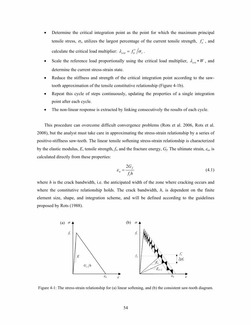
54

• Determine the critical integration point as the point for which the maximum principal

tensile stress, σt, utilizes the largest percentage of the current tensile strength, +tif , and

calculate the critical load multiplier: +=crit ti tfλ σ .

• Scale the reference load proportionally using the critical load multiplier, ∗crit Wλ , and

determine the current stress-strain state.

• Reduce the stiffness and strength of the critical integration point according to the saw-

tooth approximation of the tensile constitutive relationship (Figure 4-1b).

• Repeat this cycle of steps continuously, updating the properties of a single integration

point after each cycle.

• The non-linear response is extracted by linking consecutively the results of each cycle.

This procedure can overcome difficult convergence problems (Rots et al. 2006, Rots et al.

2008), but the analyst must take care in approximating the stress-strain relationship by a series of

positive-stiffness saw-teeth. The linear tensile softening stress-strain relationship is characterized

by the elastic modulus, E, tensile strength, ft, and the fracture energy, Gf. The ultimate strain, εu, is

calculated directly from these properties:

2

= fu

t

Gf h

ε (4.1)

where h is the crack bandwidth, i.e. the anticipated width of the zone where cracking occurs and

where the constitutive relationship holds. The crack bandwidth, h, is dependent on the finite

element size, shape, and integration scheme, and will be defined according to the guidelines

proposed by Rots (1988).

Figure 4-1: The stress-strain relationship for (a) linear softening, and (b) the consistent saw-tooth diagram.

(b) (a)

E

εu ε

ft

fG h

σ

Ei

ft

σ

Ei+1

2pft tif +

tif

εu ε

55

Several saw-tooth approximations could be specified by adjusting the elasticity, maximum

strain, and strength of each consecutive saw-tooth. However, the approximation must yield results

that are mesh independent. Rots and Invernizzi (2004) investigated several saw-tooth

approximations, and concluded that any approximation must conserve the dissipated energy, i.e.

the area under the softening curve, Gf / h. Rots et al. (2008) conducted a more expansive study

regarding the shape of the saw-tooth curve, and presented the “ripple” softening curve which was

used in this study (Figure 4-1b).

The ripple curve is derived by defining an envelope around the softening curve of magnitude

2pft (Figure 4-1b), from which the number of teeth and the reduced strength and stiffness of each

tooth are directly defined (see Rots et al. (2008) for the complete derivation). Thus, p is an input

variable which modulates the fineness of the saw-tooth approximation. While a small p value

provides more accurate results, this benefit must be balanced with the resulting increased

computational time. In the ripple curve, the dissipated energy is conserved, as over- and under-

estimation of the dissipated energy are canceled out by consecutive teeth. This is visually evident

in Figure 4-1b where the pairs of black triangles, above and below the softening curve, are of

equal area.

4.3 Non-proportional Loading

In this section, the SLA framework is extended to non-proportional loading, which opens the

door to an array of engineering applications. This extension allows the inclusion of self-weight,

which is critical when modeling full-scale structures. This is of particular interest for seismic

assessment, where self-weight can not be neglected when applying a quasi-static horizontal

loading as a first-order approximation of expected seismic loads.

A pre-stressed four-point bending beam example is used to clarify the procedure. Application

of non-proportional loading often leads to significant stress rotations, making the material

behavior in the crack parallel direction more important. As a result, an isotropic cracking model is

insufficient, and a fixed direction orthotropic cracking model is introduced. Simulations of

experimental tests with non-proportional loading by Nooru-Mohammed (Nooru-Mohammed

1992, Nooru-Mohammed et al. 1993) and Swartz and Taha (1991) are conducted to verify

accuracy and exemplify modeling capabilities and limitations.

As described in §4.2, sequentially linear analysis relies on the identification of a critical

integration point at which cracking will occur. After identification, the applied load is scaled so

56

that the critical point reaches its strength limit, its material properties are reduced, and the process

is repeated. The same process holds true for non-proportional loading, but identification of the

critical load multiplier, λcrit, becomes more complex, and universal rules for the determination of

λcrit are more difficult to derive.

4.3.1 General Procedure for Non-proportional Loading

Non-proportional loading will be described by the application of two load cases, an initial

load A and a subsequent load B, which will be superimposed. For example, load A might

represent the self-weight of the structure, and load B might represent wind or earthquake loading.

Cracking will be limited to occur during application of load B; the effect of this assumption will

be discussed later. In general, the procedure is similar to proportional loading, but specifically is

as follows:

• Apply load A, calculate the stresses, σA, and then remove load A.

• Apply a reference load B and calculate the stresses, σB.

• Calculate the load multipliers, λ1,2 , at which the maximum principal stress resulting from

the combination of loads A and B (σA + λ1,2σB ) equals the current tensile strength, +tif .

• Determine the critical integration point and calculate λcrit.

• Apply the critical load combination by scaling the reference load B with the critical load

multiplier, σA +λcritσB, and obtain the current stress-strain state.

• Remove all loads and update the stiffness and strength properties of the critical

integration point according to the saw-tooth constitutive model (Figure 4.1).

• Repeat this cycle of steps continuously, updating the properties of a single integration

point after each cycle.

These steps were implemented in an adapted version of DIANA (www.tnodiana.com) and are

described in more detail in the following sections.

Calculation of the Load Multiplier, λ

To calculate the load multiplier at each integration point, the principal stresses must be

calculated, and the maximum principal stress determined. The stresses at any integration point

can be written as:

57

, ,

, ,

, ,

= +

= +

= +

xx xx A xx B

yy yy A yy B

xy xy A xy B

σ σ λσ

σ σ λσ

σ σ λσ

(4.2)

where σ--,A represent stresses resulting from the full application of load A, and σ--,B represent

stresses resulting from the prescribed reference load B. For plane stress conditions, the principal

stresses (σ1,2) are described in the traditional manner using Equation (4.2):

( ) ( )

( ) ( ) ( )

1,2 , 1,2 , , 1,2 ,

2 2

, 1,2 , , 1,2 , , 1,2 ,

12

14

⎡ ⎤= + + + ±⎣ ⎦

⎡ ⎤+ − + + +⎣ ⎦

xx A xx B yy A yy B

xx A xx B yy A yy B xy A xy B

σ σ λ σ σ λ σ

σ λ σ σ λ σ σ λ σ (4.3)

To determine the load multipliers (λ1,2) for each integration point, the principal stresses (σ1,2)

are set equal to the current tensile strength, +tif , and Eq. (4.3) is solved for λ1,2. The closed form

solution resembles the quadratic formula:

( )21,2

1 42

= − ± −B B ACA

λ (4.4)

where:

( )( ) ( )

2, , ,

, , , , , , , ,

22, , , , ,

2+

+ +

= −

= + + − −

= − + + −

xy B xx B yy B

ti xx B yy B xy A xy B xx A yy B xx B yy A

xy A xx A yy A ti xx A yy A ti

A

B f

C f f

σ σ σ

σ σ σ σ σ σ σ σ

σ σ σ σ σ

(4.5)

Note that when ByyBxxBxy ,,, σσσ = a singularity (A = 0) occurs in Equation (4.4), and the

single solution becomes:

= −C Bλ (4.6)

The principal stress directions, 1,2ϕ , corresponding to the load multipliers, 1,2λ , must be

calculated to determine the orientation associated with each possible crack. Principal stress

directions are again calculated in the traditional manner using Equation (4.2):

( )

( ) ( ), 1,2 ,1

1,2, 1,2 , , 1,2 ,

21 tan2

−⎛ ⎞+⎜ ⎟=⎜ ⎟+ − +⎝ ⎠

xy A xy B

xx A xx B yy A yy B

σ λ σϕ

σ λ σ σ λ σ (4.7)

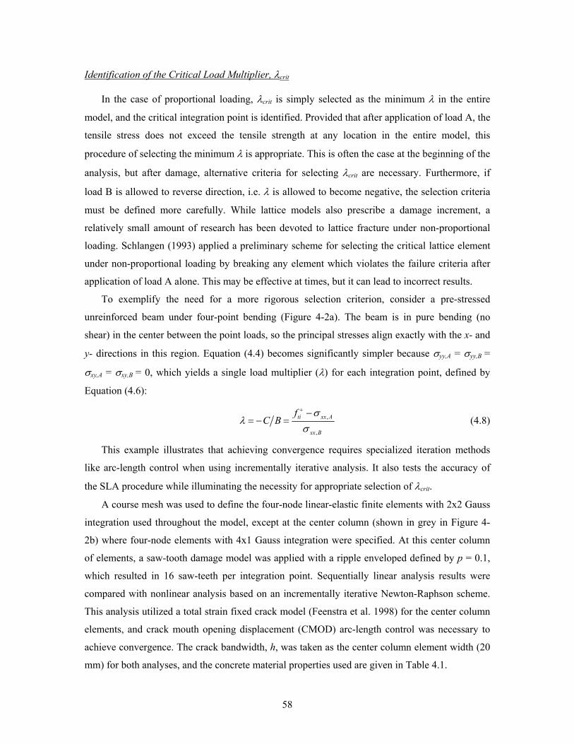
58

Identification of the Critical Load Multiplier, λcrit

In the case of proportional loading, λcrit is simply selected as the minimum λ in the entire

model, and the critical integration point is identified. Provided that after application of load A, the

tensile stress does not exceed the tensile strength at any location in the entire model, this

procedure of selecting the minimum λ is appropriate. This is often the case at the beginning of the

analysis, but after damage, alternative criteria for selecting λcrit are necessary. Furthermore, if

load B is allowed to reverse direction, i.e. λ is allowed to become negative, the selection criteria

must be defined more carefully. While lattice models also prescribe a damage increment, a

relatively small amount of research has been devoted to lattice fracture under non-proportional

loading. Schlangen (1993) applied a preliminary scheme for selecting the critical lattice element

under non-proportional loading by breaking any element which violates the failure criteria after

application of load A alone. This may be effective at times, but it can lead to incorrect results.

To exemplify the need for a more rigorous selection criterion, consider a pre-stressed

unreinforced beam under four-point bending (Figure 4-2a). The beam is in pure bending (no

shear) in the center between the point loads, so the principal stresses align exactly with the x- and

y- directions in this region. Equation (4.4) becomes significantly simpler because σyy,A = σyy,B =

σxy,A = σxy,B = 0, which yields a single load multiplier (λ) for each integration point, defined by

Equation (4.6):

,

,

+ −= − = ti xx A

xx B

fC B

σλ

σ (4.8)

This example illustrates that achieving convergence requires specialized iteration methods

like arc-length control when using incrementally iterative analysis. It also tests the accuracy of

the SLA procedure while illuminating the necessity for appropriate selection of λcrit.

A course mesh was used to define the four-node linear-elastic finite elements with 2x2 Gauss

integration used throughout the model, except at the center column (shown in grey in Figure 4-

2b) where four-node elements with 4x1 Gauss integration were specified. At this center column

of elements, a saw-tooth damage model was applied with a ripple enveloped defined by p = 0.1,

which resulted in 16 saw-teeth per integration point. Sequentially linear analysis results were

compared with nonlinear analysis based on an incrementally iterative Newton-Raphson scheme.

This analysis utilized a total strain fixed crack model (Feenstra et al. 1998) for the center column

elements, and crack mouth opening displacement (CMOD) arc-length control was necessary to

achieve convergence. The crack bandwidth, h, was taken as the center column element width (20

mm) for both analyses, and the concrete material properties used are given in Table 4.1.

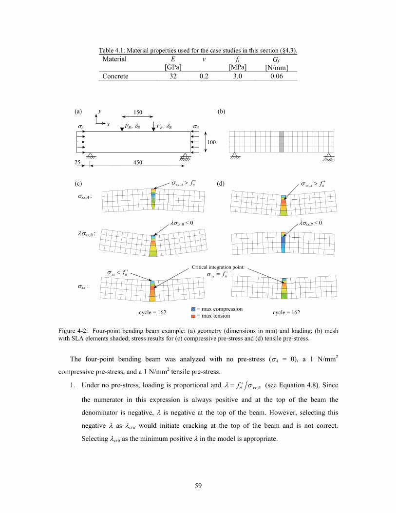
59

Table 4.1: Material properties used for the case studies in this section (§4.3). Material E

[GPa] v ft

[MPa] Gf

[N/mm] Concrete 32 0.2 3.0 0.06

Figure 4-2: Four-point bending beam example: (a) geometry (dimensions in mm) and loading; (b) mesh with SLA elements shaded; stress results for (c) compressive pre-stress and (d) tensile pre-stress.

The four-point bending beam was analyzed with no pre-stress (σA = 0), a 1 N/mm2

compressive pre-stress, and a 1 N/mm2 tensile pre-stress:

1. Under no pre-stress, loading is proportional and ,+= ti xx Bfλ σ (see Equation 4.8). Since

the numerator in this expression is always positive and at the top of the beam the

denominator is negative, λ is negative at the top of the beam. However, selecting this

negative λ as λcrit would initiate cracking at the top of the beam and is not correct.

Selecting λcrit as the minimum positive λ in the model is appropriate.

FB , δB FB , δB

450

100

150

σA σA

25

(a) (b)

(c) (d)

x

y

Critical integration point:

cycle = 162 = max compression = max tension

σxx,A :

λσxx,B :

σxx :

λσxx,B < 0 λσxx,B < 0

cycle = 162

,xx A tifσ +>,xx A tifσ +>

xx tifσ +< xx tifσ +=

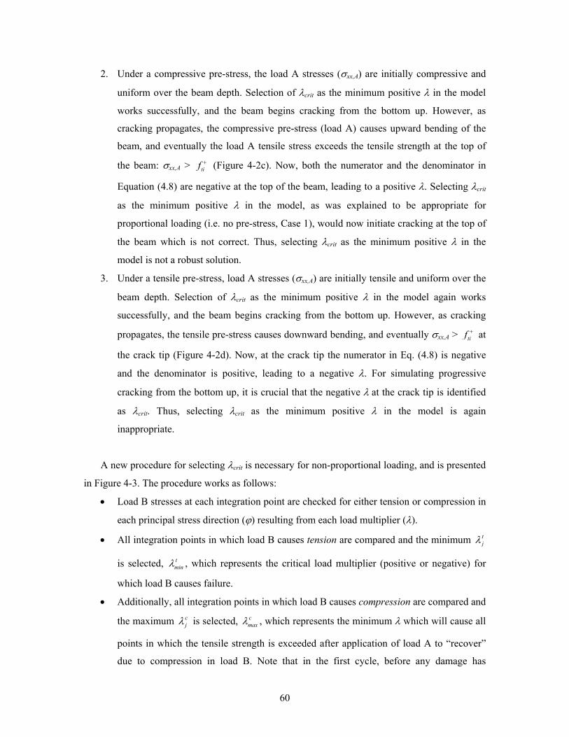
60

2. Under a compressive pre-stress, the load A stresses (σxx,A) are initially compressive and

uniform over the beam depth. Selection of λcrit as the minimum positive λ in the model

works successfully, and the beam begins cracking from the bottom up. However, as

cracking propagates, the compressive pre-stress (load A) causes upward bending of the

beam, and eventually the load A tensile stress exceeds the tensile strength at the top of

the beam: σxx,A > +tif (Figure 4-2c). Now, both the numerator and the denominator in

Equation (4.8) are negative at the top of the beam, leading to a positive λ. Selecting λcrit

as the minimum positive λ in the model, as was explained to be appropriate for

proportional loading (i.e. no pre-stress, Case 1), would now initiate cracking at the top of

the beam which is not correct. Thus, selecting λcrit as the minimum positive λ in the

model is not a robust solution.

3. Under a tensile pre-stress, load A stresses (σxx,A) are initially tensile and uniform over the

beam depth. Selection of λcrit as the minimum positive λ in the model again works

successfully, and the beam begins cracking from the bottom up. However, as cracking

propagates, the tensile pre-stress causes downward bending, and eventually σxx,A > +tif at

the crack tip (Figure 4-2d). Now, at the crack tip the numerator in Eq. (4.8) is negative

and the denominator is positive, leading to a negative λ. For simulating progressive

cracking from the bottom up, it is crucial that the negative λ at the crack tip is identified

as λcrit. Thus, selecting λcrit as the minimum positive λ in the model is again

inappropriate.

A new procedure for selecting λcrit is necessary for non-proportional loading, and is presented

in Figure 4-3. The procedure works as follows:

• Load B stresses at each integration point are checked for either tension or compression in

each principal stress direction (ϕ) resulting from each load multiplier (λ).

• All integration points in which load B causes tension are compared and the minimum tjλ

is selected, tminλ , which represents the critical load multiplier (positive or negative) for

which load B causes failure.

• Additionally, all integration points in which load B causes compression are compared and

the maximum cjλ is selected, c

maxλ , which represents the minimum λ which will cause all

points in which the tensile strength is exceeded after application of load A to “recover”

due to compression in load B. Note that in the first cycle, before any damage has

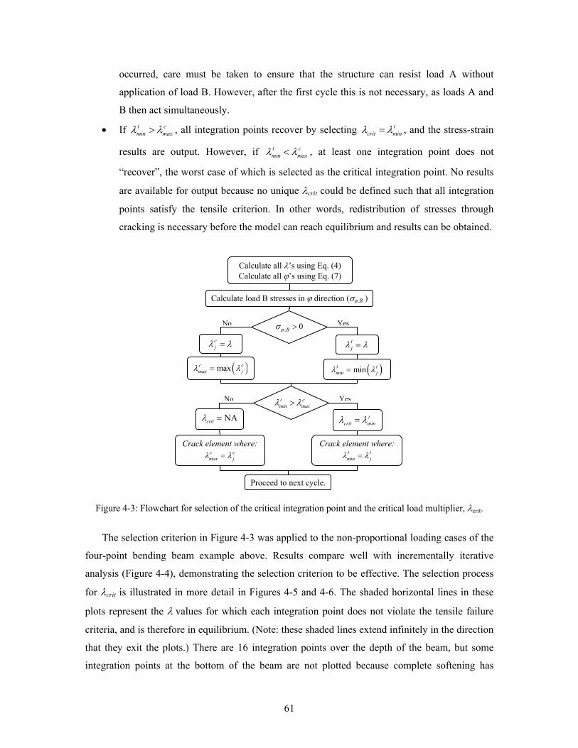
61

occurred, care must be taken to ensure that the structure can resist load A without

application of load B. However, after the first cycle this is not necessary, as loads A and

B then act simultaneously.

• If >t cmin maxλ λ , all integration points recover by selecting = t

crit minλ λ , and the stress-strain

results are output. However, if <t cmin maxλ λ , at least one integration point does not

“recover”, the worst case of which is selected as the critical integration point. No results

are available for output because no unique λcrit could be defined such that all integration

points satisfy the tensile criterion. In other words, redistribution of stresses through

cracking is necessary before the model can reach equilibrium and results can be obtained.

Figure 4-3: Flowchart for selection of the critical integration point and the critical load multiplier, λcrit.

The selection criterion in Figure 4-3 was applied to the non-proportional loading cases of the

four-point bending beam example above. Results compare well with incrementally iterative

analysis (Figure 4-4), demonstrating the selection criterion to be effective. The selection process

for λcrit is illustrated in more detail in Figures 4-5 and 4-6. The shaded horizontal lines in these

plots represent the λ values for which each integration point does not violate the tensile failure

criteria, and is therefore in equilibrium. (Note: these shaded lines extend infinitely in the direction

that they exit the plots.) There are 16 integration points over the depth of the beam, but some

integration points at the bottom of the beam are not plotted because complete softening has

Calculate load B stresses in ϕ direction (σϕ,B )

Calculate all λ’s using Eq. (4) Calculate all ϕ’s using Eq. (7)

( )mint tmin jλ λ=

cjλ λ=

( )maxc cmax jλ λ=

Proceed to next cycle.

tjλ λ=

tcrit minλ λ=

t cmin maxλ λ>

, 0Bϕσ >

YesNo

NAcritλ =

Crack element where: t tmin jλ λ=

Crack element where: c cmax jλ λ=

No Yes

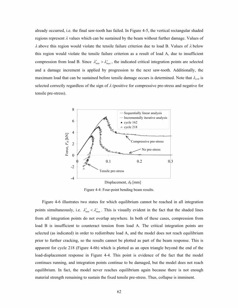
62

already occurred, i.e. the final saw-tooth has failed. In Figure 4-5, the vertical rectangular shaded

regions represent λ values which can be sustained by the beam without further damage. Values of

λ above this region would violate the tensile failure criterion due to load B. Values of λ below

this region would violate the tensile failure criterion as a result of load A, due to insufficient

compression from load B. Since >t cmin maxλ λ , the indicated critical integration points are selected

and a damage increment is applied by progression to the next saw-tooth. Additionally, the

maximum load that can be sustained before tensile damage occurs is determined. Note that λcrit is

selected correctly regardless of the sign of λ (positive for compressive pre-stress and negative for

tensile pre-stress).

Figure 4-4: Four-point bending beam results.

Figure 4-6 illustrates two states for which equilibrium cannot be reached in all integration

points simultaneously, i.e. <t cmin maxλ λ . This is visually evident in the fact that the shaded lines

from all integration points do not overlap anywhere. In both of these cases, compression from

load B is insufficient to counteract tension from load A. The critical integration points are

selected (as indicated) in order to redistribute load A, and the model does not reach equilibrium

prior to further cracking, so the results cannot be plotted as part of the beam response. This is

apparent for cycle 218 (Figure 4-6b) which is plotted as an open triangle beyond the end of the

load-displacement response in Figure 4-4. This point is evidence of the fact that the model

continues running, and integration points continue to be damaged, but the model does not reach

equilibrium. In fact, the model never reaches equilibrium again because there is not enough

material strength remaining to sustain the fixed tensile pre-stress. Thus, collapse is imminent.

-4

-2

0

2

4

6

8

0 0.1 0.2 0.3

Sequentially linear analysisIncrementally iterative analysiscycle 162cycle 218

Compressive pre-stress

No pre-stress

Tensile pre-stress

Forc

e, F

B [kN

]

Displacement, δB [mm]

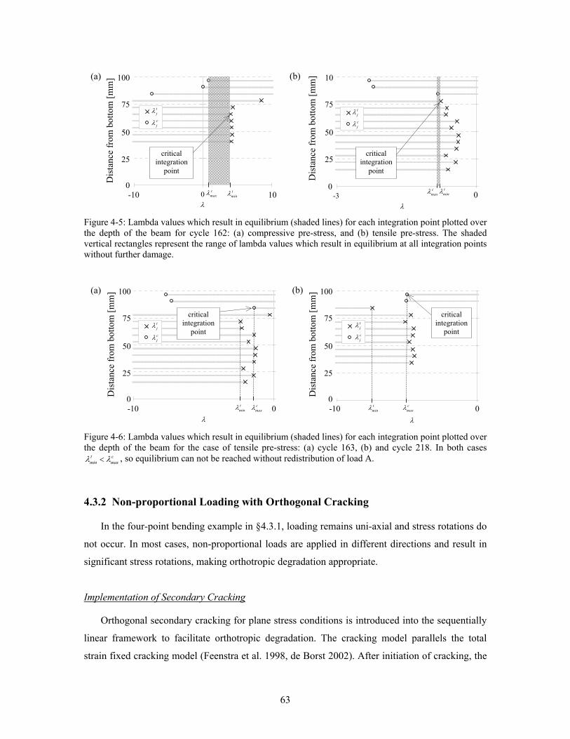
63

Figure 4-5: Lambda values which result in equilibrium (shaded lines) for each integration point plotted over the depth of the beam for cycle 162: (a) compressive pre-stress, and (b) tensile pre-stress. The shaded vertical rectangles represent the range of lambda values which result in equilibrium at all integration points without further damage.

Figure 4-6: Lambda values which result in equilibrium (shaded lines) for each integration point plotted over the depth of the beam for the case of tensile pre-stress: (a) cycle 163, (b) and cycle 218. In both cases

<t cmin maxλ λ , so equilibrium can not be reached without redistribution of load A.

4.3.2 Non-proportional Loading with Orthogonal Cracking

In the four-point bending example in §4.3.1, loading remains uni-axial and stress rotations do

not occur. In most cases, non-proportional loads are applied in different directions and result in

significant stress rotations, making orthotropic degradation appropriate.

Implementation of Secondary Cracking

Orthogonal secondary cracking for plane stress conditions is introduced into the sequentially

linear framework to facilitate orthotropic degradation. The cracking model parallels the total

strain fixed cracking model (Feenstra et al. 1998, de Borst 2002). After initiation of cracking, the

(a)

0

25

50

75

100

-3 0λ

Dis

tanc

e fro

m b

otto

m [m

m]

critical integration

point

tminλ c

maxλ0

25

50

75

100

-4 0λ

Dis

tanc

e fro

m b

otto

m [m

m]


point

cmaxλ t

minλ

100

75

50

25

0 -10

Dis

tanc

e fr

om b

otto

m [m

m]

0

100

75

50

25

0-10

Dis

tanc

e fr

om b

otto

m [m

m]

0

tj

cj

λ

λ

tj

cj

λ

λ

0

25

50

75

100

-3 0λ

Dis

tanc

e fro

m b

otto

m [m

m]


point

(a) (b)

0

25

50

75

100

-10 0 10λ

Dis

tanc

e fro

m b

otto

m [m

m]


point

tj

cj

λ

λ

tminλc

maxλ tminλ c

maxλ

100

75

50

25

0 -10 100

10

75

50

25

0-3 0

Dis

tanc

e fr

om b

otto

m [m

m]

Dis

tanc

e fr

om b

otto

m [m

m]

0

tj

cj

λ

λ

(b)

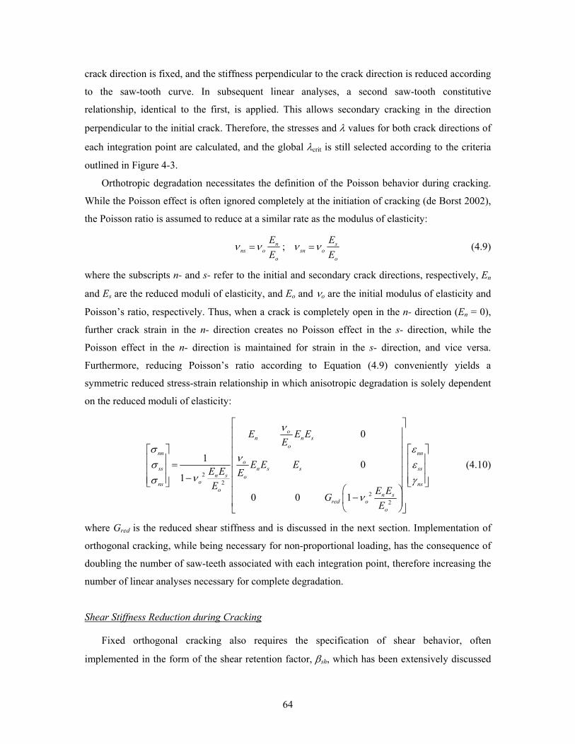
64

crack direction is fixed, and the stiffness perpendicular to the crack direction is reduced according

to the saw-tooth curve. In subsequent linear analyses, a second saw-tooth constitutive

relationship, identical to the first, is applied. This allows secondary cracking in the direction

perpendicular to the initial crack. Therefore, the stresses and λ values for both crack directions of

each integration point are calculated, and the global λcrit is still selected according to the criteria

outlined in Figure 4-3.

Orthotropic degradation necessitates the definition of the Poisson behavior during cracking.

While the Poisson effect is often ignored completely at the initiation of cracking (de Borst 2002),

the Poisson ratio is assumed to reduce at a similar rate as the modulus of elasticity:

;= =n sns o sn o

o o

E EE E

ν ν ν ν (4.9)

where the subscripts n- and s- refer to the initial and secondary crack directions, respectively, En

and Es are the reduced moduli of elasticity, and Eo and νo are the initial modulus of elasticity and

Poisson’s ratio, respectively. Thus, when a crack is completely open in the n- direction (En = 0),

further crack strain in the n- direction creates no Poisson effect in the s- direction, while the

Poisson effect in the n- direction is maintained for strain in the s- direction, and vice versa.

Furthermore, reducing Poisson’s ratio according to Equation (4.9) conveniently yields a

symmetric reduced stress-strain relationship in which anisotropic degradation is solely dependent

on the reduced moduli of elasticity:

2

2

22

0

1 01

0 0 1

⎡ ⎤⎢ ⎥⎢ ⎥

⎡ ⎤ ⎡ ⎤⎢ ⎥⎢ ⎥ ⎢ ⎥⎢ ⎥=⎢ ⎥ ⎢ ⎥⎢ ⎥−⎢ ⎥ ⎢ ⎥⎢ ⎥⎣ ⎦ ⎣ ⎦

⎛ ⎞⎢ ⎥−⎜ ⎟⎢ ⎥⎝ ⎠⎣ ⎦

on n s

onn nn

oss n s s ss

n s oons ns

on s

red oo

E E EE

E E EE E EE E EG

E

ν

σ εν

σ ενσ γ

ν

(4.10)

where Gred is the reduced shear stiffness and is discussed in the next section. Implementation of

orthogonal cracking, while being necessary for non-proportional loading, has the consequence of

doubling the number of saw-teeth associated with each integration point, therefore increasing the

number of linear analyses necessary for complete degradation.

Shear Stiffness Reduction during Cracking

Fixed orthogonal cracking also requires the specification of shear behavior, often

implemented in the form of the shear retention factor, βsh, which has been extensively discussed

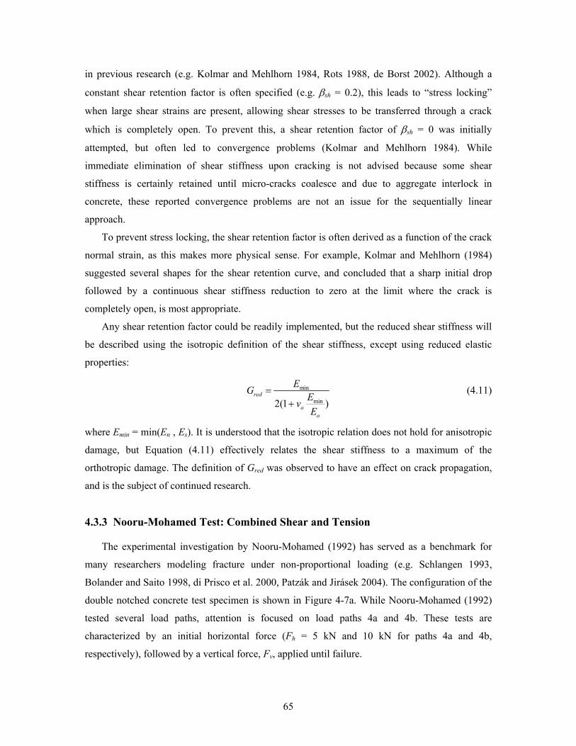
65

in previous research (e.g. Kolmar and Mehlhorn 1984, Rots 1988, de Borst 2002). Although a

constant shear retention factor is often specified (e.g. βsh = 0.2), this leads to “stress locking”

when large shear strains are present, allowing shear stresses to be transferred through a crack

which is completely open. To prevent this, a shear retention factor of βsh = 0 was initially

attempted, but often led to convergence problems (Kolmar and Mehlhorn 1984). While

immediate elimination of shear stiffness upon cracking is not advised because some shear

stiffness is certainly retained until micro-cracks coalesce and due to aggregate interlock in

concrete, these reported convergence problems are not an issue for the sequentially linear

approach.

To prevent stress locking, the shear retention factor is often derived as a function of the crack

normal strain, as this makes more physical sense. For example, Kolmar and Mehlhorn (1984)

suggested several shapes for the shear retention curve, and concluded that a sharp initial drop

followed by a continuous shear stiffness reduction to zero at the limit where the crack is

completely open, is most appropriate.

Any shear retention factor could be readily implemented, but the reduced shear stiffness will

be described using the isotropic definition of the shear stiffness, except using reduced elastic

properties:

min

min2(1 )=

+red

oo

EG EvE

(4.11)

where Emin = min(En , Es). It is understood that the isotropic relation does not hold for anisotropic

damage, but Equation (4.11) effectively relates the shear stiffness to a maximum of the

orthotropic damage. The definition of Gred was observed to have an effect on crack propagation,

and is the subject of continued research.

4.3.3 Nooru-Mohamed Test: Combined Shear and Tension

The experimental investigation by Nooru-Mohamed (1992) has served as a benchmark for

many researchers modeling fracture under non-proportional loading (e.g. Schlangen 1993,

Bolander and Saito 1998, di Prisco et al. 2000, Patzák and Jirásek 2004). The configuration of the

double notched concrete test specimen is shown in Figure 4-7a. While Nooru-Mohamed (1992)

tested several load paths, attention is focused on load paths 4a and 4b. These tests are

characterized by an initial horizontal force (Fh = 5 kN and 10 kN for paths 4a and 4b,

respectively), followed by a vertical force, Fv, applied until failure.

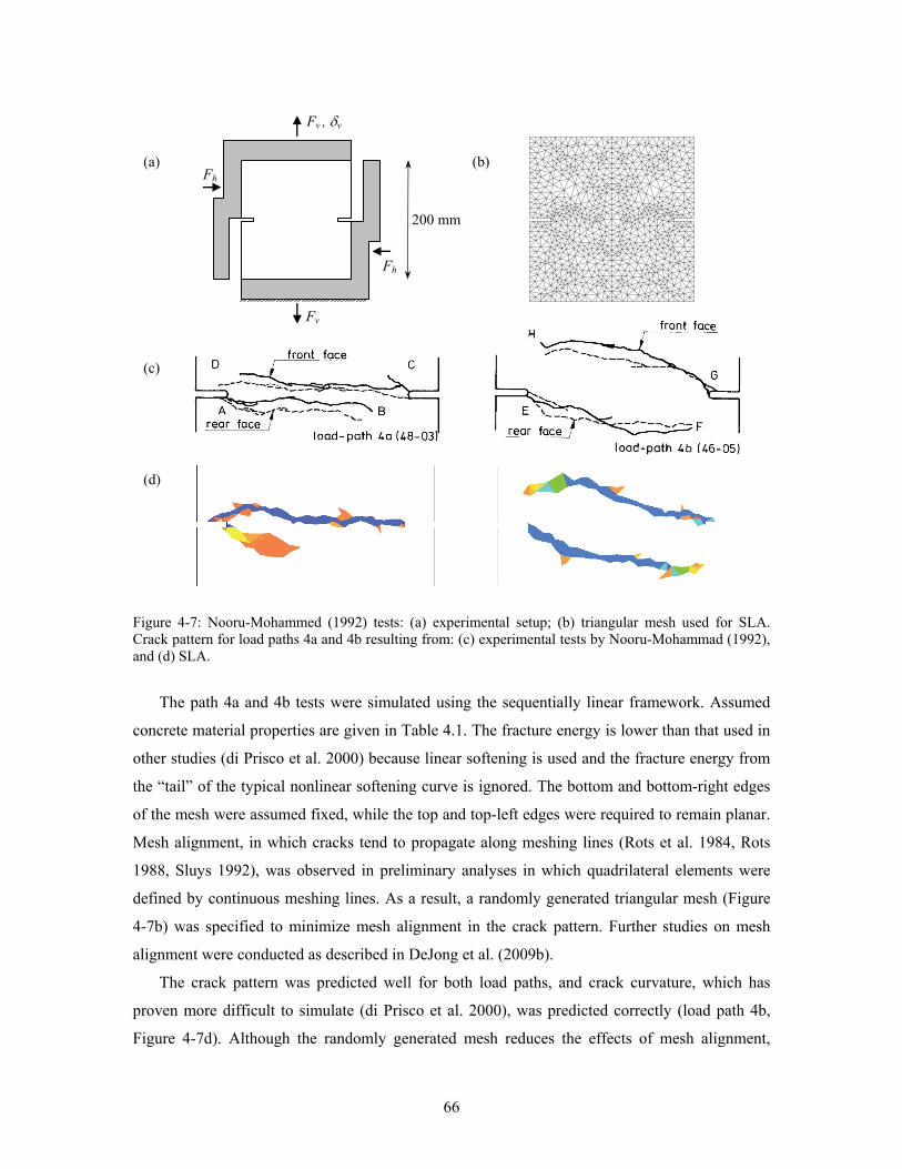
66

Figure 4-7: Nooru-Mohammed (1992) tests: (a) experimental setup; (b) triangular mesh used for SLA. Crack pattern for load paths 4a and 4b resulting from: (c) experimental tests by Nooru-Mohammad (1992), and (d) SLA.

The path 4a and 4b tests were simulated using the sequentially linear framework. Assumed

concrete material properties are given in Table 4.1. The fracture energy is lower than that used in

other studies (di Prisco et al. 2000) because linear softening is used and the fracture energy from

the “tail” of the typical nonlinear softening curve is ignored. The bottom and bottom-right edges

of the mesh were assumed fixed, while the top and top-left edges were required to remain planar.

Mesh alignment, in which cracks tend to propagate along meshing lines (Rots et al. 1984, Rots

1988, Sluys 1992), was observed in preliminary analyses in which quadrilateral elements were

defined by continuous meshing lines. As a result, a randomly generated triangular mesh (Figure

4-7b) was specified to minimize mesh alignment in the crack pattern. Further studies on mesh

alignment were conducted as described in DeJong et al. (2009b).

The crack pattern was predicted well for both load paths, and crack curvature, which has

proven more difficult to simulate (di Prisco et al. 2000), was predicted correctly (load path 4b,

Figure 4-7d). Although the randomly generated mesh reduces the effects of mesh alignment,

Fh

Fv , δv

Fh

Fv

(a) (b)

(c)

(d)

200 mm

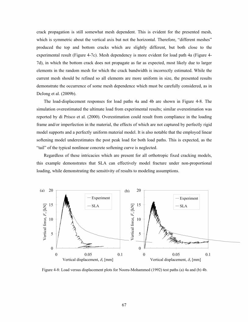
67

crack propagation is still somewhat mesh dependent. This is evident for the presented mesh,

which is symmetric about the vertical axis but not the horizontal. Therefore, “different meshes”

produced the top and bottom cracks which are slightly different, but both close to the

experimental result (Figure 4-7c). Mesh dependency is more evident for load path 4a (Figure 4-

7d), in which the bottom crack does not propagate as far as expected, most likely due to larger

elements in the random mesh for which the crack bandwidth is incorrectly estimated. While the

current mesh should be refined so all elements are more uniform in size, the presented results

demonstrate the occurrence of some mesh dependence which must be carefully considered, as in

DeJong et al. (2009b).

The load-displacement responses for load paths 4a and 4b are shown in Figure 4-8. The

simulation overestimated the ultimate load from experimental results; similar overestimation was

reported by di Prisco et al. (2000). Overestimation could result from compliance in the loading

frame and/or imperfection in the material, the effects of which are not captured by perfectly rigid

model supports and a perfectly uniform material model. It is also notable that the employed linear

softening model underestimates the post peak load for both load paths. This is expected, as the

“tail” of the typical nonlinear concrete softening curve is neglected.

Regardless of these intricacies which are present for all orthotropic fixed cracking models,

this example demonstrates that SLA can effectively model fracture under non-proportional

loading, while demonstrating the sensitivity of results to modeling assumptions.

Figure 4-8: Load versus displacement plots for Nooru-Mohammed (1992) test paths (a) 4a and (b) 4b.

0

5

10

15

20

0 0.05 0.1

Experiment

SLA

0

5

10

15

20

0 0.05 0.1

Experiment

SLA

(a) (b)

Ver

tical

forc

e, F

v [kN

]

Vertical displacement, δv [mm]

Ver

tical

forc

e, F

v [kN

]

Vertical displacement, δv [mm]

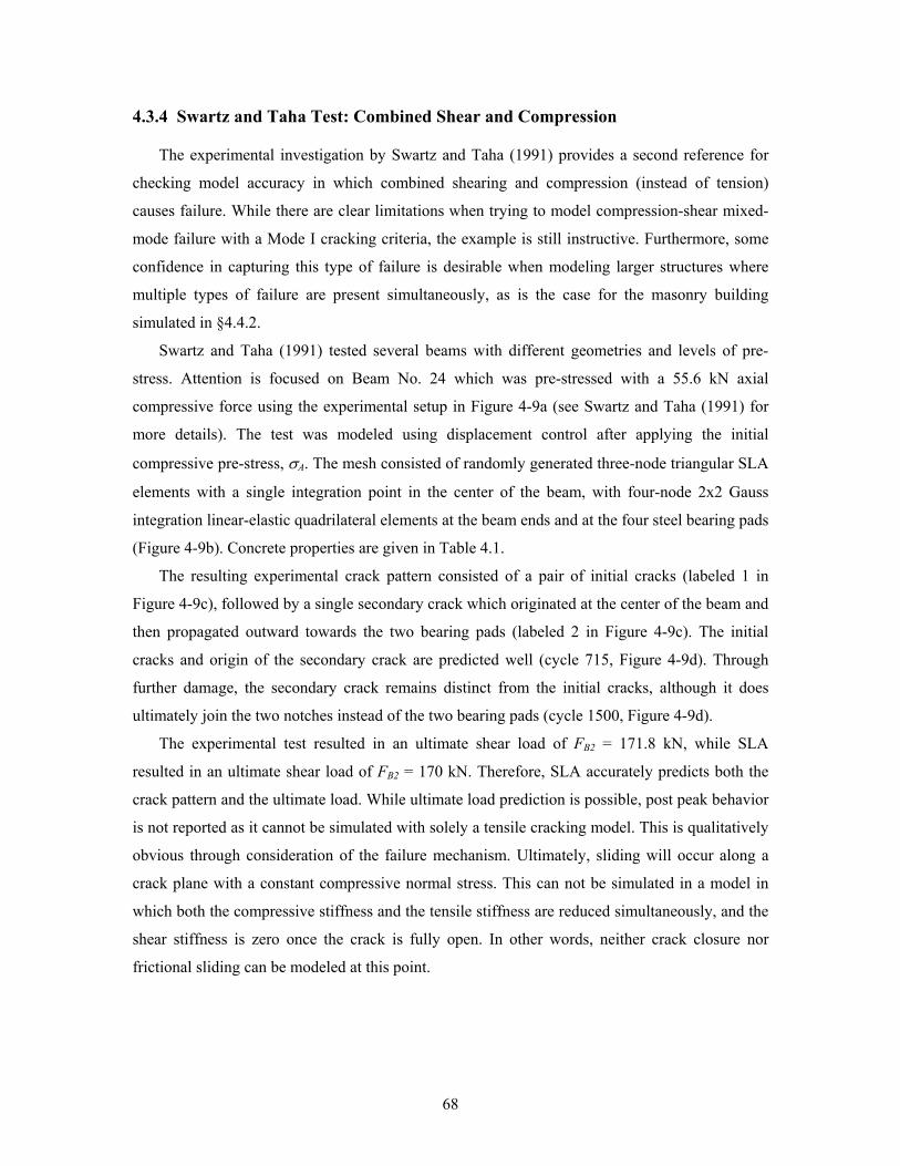
68

4.3.4 Swartz and Taha Test: Combined Shear and Compression

The experimental investigation by Swartz and Taha (1991) provides a second reference for

checking model accuracy in which combined shearing and compression (instead of tension)

causes failure. While there are clear limitations when trying to model compression-shear mixed-

mode failure with a Mode I cracking criteria, the example is still instructive. Furthermore, some

confidence in capturing this type of failure is desirable when modeling larger structures where

multiple types of failure are present simultaneously, as is the case for the masonry building

simulated in §4.4.2.

Swartz and Taha (1991) tested several beams with different geometries and levels of pre-

stress. Attention is focused on Beam No. 24 which was pre-stressed with a 55.6 kN axial

compressive force using the experimental setup in Figure 4-9a (see Swartz and Taha (1991) for

more details). The test was modeled using displacement control after applying the initial

compressive pre-stress, σA. The mesh consisted of randomly generated three-node triangular SLA

elements with a single integration point in the center of the beam, with four-node 2x2 Gauss

integration linear-elastic quadrilateral elements at the beam ends and at the four steel bearing pads

(Figure 4-9b). Concrete properties are given in Table 4.1.

The resulting experimental crack pattern consisted of a pair of initial cracks (labeled 1 in

Figure 4-9c), followed by a single secondary crack which originated at the center of the beam and

then propagated outward towards the two bearing pads (labeled 2 in Figure 4-9c). The initial

cracks and origin of the secondary crack are predicted well (cycle 715, Figure 4-9d). Through

further damage, the secondary crack remains distinct from the initial cracks, although it does

ultimately join the two notches instead of the two bearing pads (cycle 1500, Figure 4-9d).

The experimental test resulted in an ultimate shear load of FB2 = 171.8 kN, while SLA

resulted in an ultimate shear load of FB2 = 170 kN. Therefore, SLA accurately predicts both the

crack pattern and the ultimate load. While ultimate load prediction is possible, post peak behavior

is not reported as it cannot be simulated with solely a tensile cracking model. This is qualitatively

obvious through consideration of the failure mechanism. Ultimately, sliding will occur along a

crack plane with a constant compressive normal stress. This can not be simulated in a model in

which both the compressive stiffness and the tensile stiffness are reduced simultaneously, and the

shear stiffness is zero once the crack is fully open. In other words, neither crack closure nor

frictional sliding can be modeled at this point.

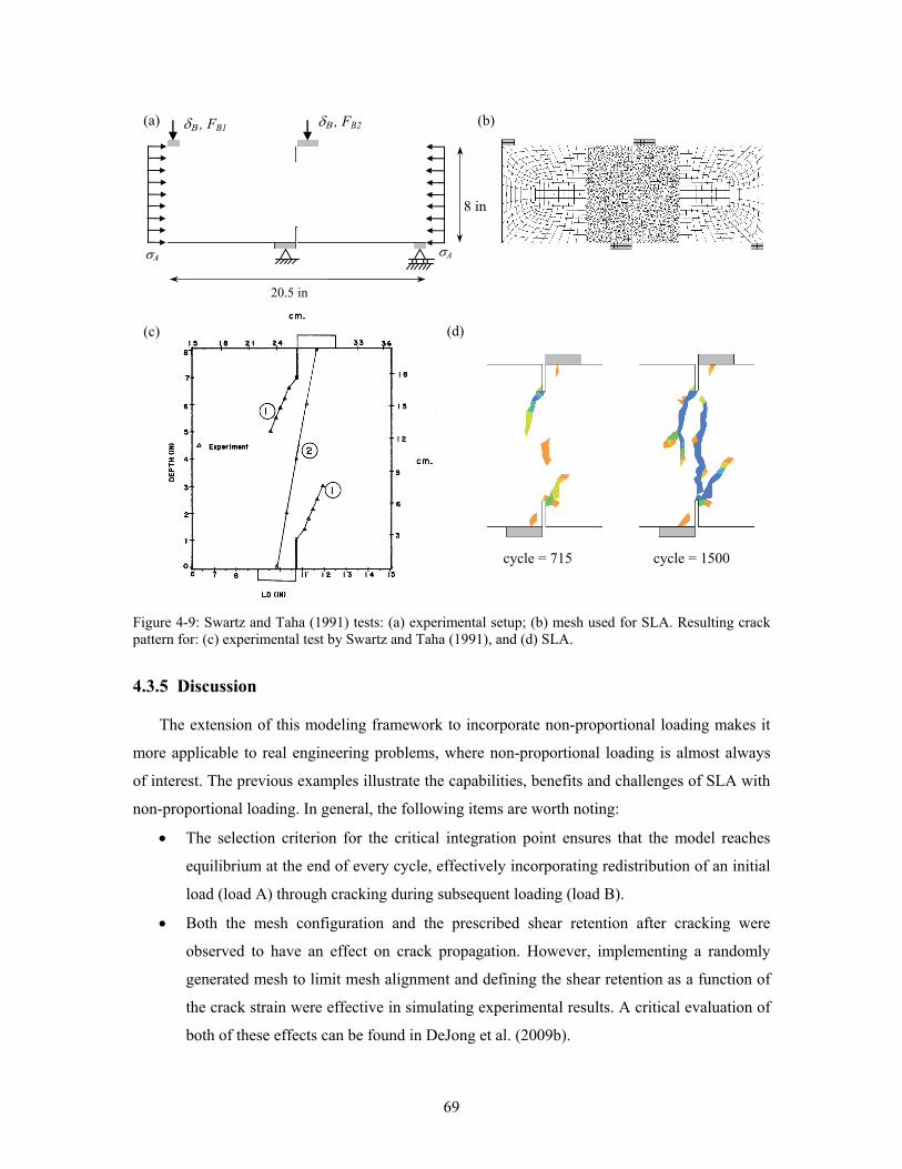
69

Figure 4-9: Swartz and Taha (1991) tests: (a) experimental setup; (b) mesh used for SLA. Resulting crack pattern for: (c) experimental test by Swartz and Taha (1991), and (d) SLA.

4.3.5 Discussion

The extension of this modeling framework to incorporate non-proportional loading makes it

more applicable to real engineering problems, where non-proportional loading is almost always

of interest. The previous examples illustrate the capabilities, benefits and challenges of SLA with

non-proportional loading. In general, the following items are worth noting:

• The selection criterion for the critical integration point ensures that the model reaches

equilibrium at the end of every cycle, effectively incorporating redistribution of an initial

load (load A) through cracking during subsequent loading (load B).

• Both the mesh configuration and the prescribed shear retention after cracking were

observed to have an effect on crack propagation. However, implementing a randomly

generated mesh to limit mesh alignment and defining the shear retention as a function of

the crack strain were effective in simulating experimental results. A critical evaluation of

both of these effects can be found in DeJong et al. (2009b).

(a) (b)

(c) (d)

δΒ , FB2

8 in

σA

δΒ , FB1

σA

20.5 in

cycle = 1500 cycle = 715

70

• The primary advantage of the SLA method is its ability to model brittle behavior without

convergence problems. This benefit is particularly important when modeling fracture in

large-scale structures where brittle snap-back behavior is amplified (DeJong et al. 2008).

While SLA is effective for many applications, clear limitations exist. For example, the

inability to model crack closure and subsequent frictional sliding has not yet been addressed.

Additionally, run-times can be long for models where a large number of integration points are

present, especially if the modeling framework is extended to 3D brick elements in the future.

However, more efficient solution techniques could be developed which significantly reduce run-

times.

4.4 Shell Structures

The previous section has exemplified some of the intricacies of simulating brittle fracture

under non-proportional loading using the SLA method. In fact, the method effectively matches

the capabilities of total strain fixed crack models (e.g. Feenstra 1998), with the enormous benefit

of eliminating convergence problems. Although many methods have been developed to deal with

convergence issues, this primary advantage of the sequentially linear method is more evident

when modeling fracture of full-scale structures. In this section, shell elements are incorporated

into the sequentially linear analysis method to allow the modeling of three dimensional masonry

structures under non-proportional loading. In the following sections, the shell element

implementation is first presented and then applied to simulate a previous experimental test on a

full-scale masonry structure under cyclic loading.

4.4.1 Implementation of Shell Elements in SLA

The capability of SLA is extended to three dimensional structures through the use of shell

elements. While analysis with full 3D solid elements is possible, shell elements provide an

efficient means of modeling many typical structures. The general solution procedure is the same

as in two dimensions, as presented in the previous sections.

Shell elements are typically utilized in finite element analysis when structures are thin in one

dimension, as is often the case in walls, floors, and roofs of buildings. They provide an efficient

means of modeling 3D structures without 3D solid finite elements, which complicate and slow

analyses if they are not necessary. In this formulation, Mindlin-Reissner shell theory is applied, in

which the stress through the thickness (perpendicular to the mid-surface of the plate or shell) is

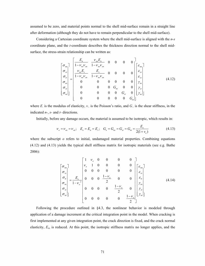
71

assumed to be zero, and material points normal to the shell mid-surface remain in a straight line

after deformation (although they do not have to remain perpendicular to the shell mid-surface).

Considering a Cartesian coordinate system where the shell mid-surface is aligned with the n-s

coordinate plane, and the t-coordinate describes the thickness direction normal to the shell mid-

surface, the stress-strain relationship can be written as:

0 0 0 01 1

0 0 0 01 1

0 0 0 0 0 00 0 0 0 00 0 0 0 00 0 0 0 0

⎡ ⎤⎢ ⎥− −⎡ ⎤ ⎡ ⎤⎢ ⎥⎢ ⎥ ⎢ ⎥⎢ ⎥⎢ ⎥ ⎢ ⎥⎢ ⎥⎢ ⎥ ⎢ ⎥− −⎢ ⎥=⎢ ⎥ ⎢ ⎥⎢ ⎥⎢ ⎥ ⎢ ⎥⎢ ⎥⎢ ⎥ ⎢ ⎥⎢ ⎥⎢ ⎥ ⎢ ⎥⎢ ⎥⎢ ⎥ ⎢ ⎥⎣ ⎦ ⎣ ⎦⎢ ⎥⎢ ⎥⎣ ⎦

n sn n

ns sn ns snnn nn

ss ns s s ss

ns sn ns sntt zz

ns ns

nsst st

sttn tn

tn

E E

E E

GG

G

νν ν ν νσ ε

σ ν εν ν ν νσ ε

σ γσ γσ γ

(4.12)

where E- is the modulus of elasticity, v-- is the Poisson’s ratio, and G-- is the shear stiffness, in the

indicated n-, s- and t- directions.

Initially, before any damage occurs, the material is assumed to be isotropic, which results in:

; ;2(1 )

= = = = = = = =+

oo ns sn o n s o ns st tn

o

EE E E G G G Gv

ν ν ν (4.13)

where the subscript o refers to initial, undamaged material properties. Combining equations

(4.12) and (4.13) yields the typical shell stiffness matrix for isotropic materials (see e.g. Bathe

2006):

2

1 0 0 0 01 0 0 0 0

0 0 0 0 0 010 0 0 0 0

2110 0 0 0 0

210 0 0 0 0

2

⎡ ⎤⎢ ⎥

⎡ ⎤ ⎡ ⎤⎢ ⎥⎢ ⎥ ⎢ ⎥⎢ ⎥⎢ ⎥ ⎢ ⎥⎢ ⎥−⎢ ⎥ ⎢ ⎥⎢ ⎥

=⎢ ⎥ ⎢ ⎥⎢ ⎥−⎢ ⎥ ⎢ ⎥⎢ ⎥−⎢ ⎥ ⎢ ⎥⎢ ⎥⎢ ⎥ ⎢ ⎥⎢ ⎥⎢ ⎥ ⎢ ⎥⎣ ⎦ ⎣ ⎦⎢ ⎥−

⎢ ⎥⎣ ⎦

o

onn nn

ss ss

ott tto

ns nsoo

st st

tn tno

E

ννσ ε

σ ενσ ε

σ γννσ γ

σ γν

(4.14)

Following the procedure outlined in §4.3, the nonlinear behavior is modeled through

application of a damage increment at the critical integration point in the model. When cracking is

first implemented at any given integration point, the crack direction is fixed, and the crack normal

elasticity, En, is reduced. At this point, the isotropic stiffness matrix no longer applies, and the

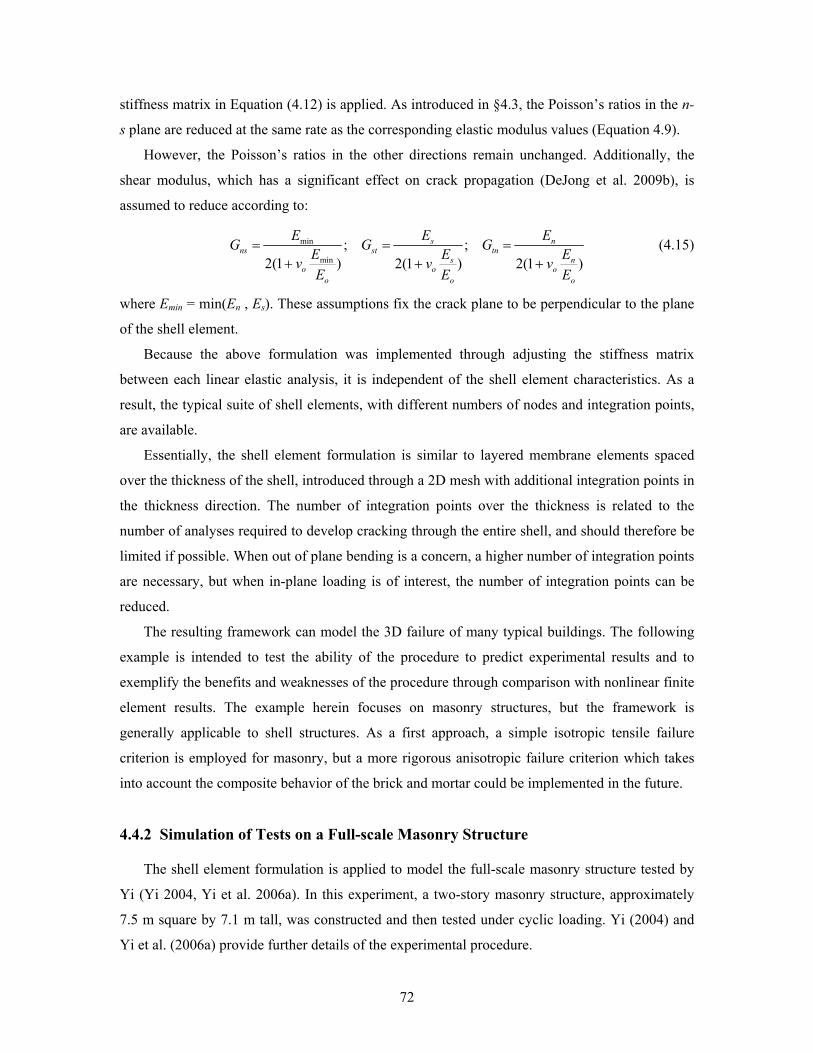
72

stiffness matrix in Equation (4.12) is applied. As introduced in §4.3, the Poisson’s ratios in the n-

s plane are reduced at the same rate as the corresponding elastic modulus values (Equation 4.9).

However, the Poisson’s ratios in the other directions remain unchanged. Additionally, the

shear modulus, which has a significant effect on crack propagation (DeJong et al. 2009b), is

assumed to reduce according to:

min

min; ;

2(1 ) 2(1 ) 2(1 )= = =

+ + +

s nns st tn

s no o o

o o o

E EEG G GE E Ev v vE E E

(4.15)

where Emin = min(En , Es). These assumptions fix the crack plane to be perpendicular to the plane

of the shell element.

Because the above formulation was implemented through adjusting the stiffness matrix

between each linear elastic analysis, it is independent of the shell element characteristics. As a

result, the typical suite of shell elements, with different numbers of nodes and integration points,

are available.

Essentially, the shell element formulation is similar to layered membrane elements spaced

over the thickness of the shell, introduced through a 2D mesh with additional integration points in

the thickness direction. The number of integration points over the thickness is related to the

number of analyses required to develop cracking through the entire shell, and should therefore be

limited if possible. When out of plane bending is a concern, a higher number of integration points

are necessary, but when in-plane loading is of interest, the number of integration points can be

reduced.

The resulting framework can model the 3D failure of many typical buildings. The following

example is intended to test the ability of the procedure to predict experimental results and to

exemplify the benefits and weaknesses of the procedure through comparison with nonlinear finite

element results. The example herein focuses on masonry structures, but the framework is

generally applicable to shell structures. As a first approach, a simple isotropic tensile failure

criterion is employed for masonry, but a more rigorous anisotropic failure criterion which takes

into account the composite behavior of the brick and mortar could be implemented in the future.

4.4.2 Simulation of Tests on a Full-scale Masonry Structure

The shell element formulation is applied to model the full-scale masonry structure tested by

Yi (Yi 2004, Yi et al. 2006a). In this experiment, a two-story masonry structure, approximately

7.5 m square by 7.1 m tall, was constructed and then tested under cyclic loading. Yi (2004) and

Yi et al. (2006a) provide further details of the experimental procedure.

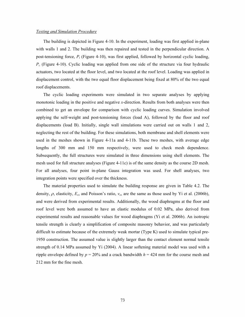
73

Testing and Simulation Procedure

The building is depicted in Figure 4-10. In the experiment, loading was first applied in-plane

with walls 1 and 2. The building was then repaired and tested in the perpendicular direction. A

post-tensioning force, Pt (Figure 4-10), was first applied, followed by horizontal cyclic loading,

Pc (Figure 4-10). Cyclic loading was applied from one side of the structure via four hydraulic

actuators, two located at the floor level, and two located at the roof level. Loading was applied in

displacement control, with the two equal floor displacement being fixed at 80% of the two equal

roof displacements.

The cyclic loading experiments were simulated in two separate analyses by applying

monotonic loading in the positive and negative x-direction. Results from both analyses were then

combined to get an envelope for comparison with cyclic loading curves. Simulation involved

applying the self-weight and post-tensioning forces (load A), followed by the floor and roof

displacements (load B). Initially, single wall simulations were carried out on walls 1 and 2,

neglecting the rest of the building. For these simulations, both membrane and shell elements were

used in the meshes shown in Figure 4-11a and 4-11b. These two meshes, with average edge

lengths of 300 mm and 150 mm respectively, were used to check mesh dependence.

Subsequently, the full structures were simulated in three dimensions using shell elements. The

mesh used for full structure analyses (Figure 4-11c) is of the same density as the course 2D mesh.

For all analyses, four point in-plane Gauss integration was used. For shell analyses, two

integration points were specified over the thickness.

The material properties used to simulate the building response are given in Table 4.2. The

density, ρ, elasticity, Eo, and Poisson’s ratio, vo, are the same as those used by Yi et al. (2006b),

and were derived from experimental results. Additionally, the wood diaphragms at the floor and

roof level were both assumed to have an elastic modulus of 0.02 MPa, also derived from

experimental results and reasonable values for wood diaphragms (Yi et al. 2006b). An isotropic

tensile strength is clearly a simplification of composite masonry behavior, and was particularly

difficult to estimate because of the extremely weak mortar (Type K) used to simulate typical pre-

1950 construction. The assumed value is slightly larger than the contact element normal tensile

strength of 0.14 MPa assumed by Yi (2004). A linear softening material model was used with a

ripple envelope defined by p = 20% and a crack bandwidth h = 424 mm for the course mesh and

212 mm for the fine mesh.

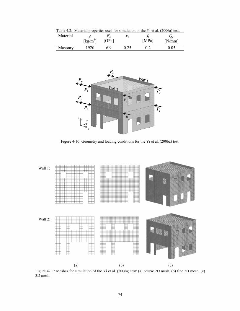
74

Table 4.2: Material properties used for simulation of the Yi et al. (2006a) test. Material ρ

[kg/m3] Eo

[GPa] vo ft

[MPa] Gf

[N/mm] Masonry 1920 6.9 0.25 0.2 0.05

Figure 4-10: Geometry and loading conditions for the Yi et al. (2006a) test.

Figure 4-11: Meshes for simulation of the Yi et al. (2006a) test: (a) course 2D mesh, (b) fine 2D mesh, (c) 3D mesh.

Wall 1:

Wall 2:

(c) (b)(a)

x

y z

Pc

Pc

Pc

Pt

Pt

Pt

Pt

Pt

Pt

Wall 1

Wall 2

Pc

Pc

Pc

Pt

Pt

Pt

Pt

Pt

Pt

Pc

Pc

Pc

Pt

Pt

Pt

Pt

Pt

Pt

Wall 1

Wall 2

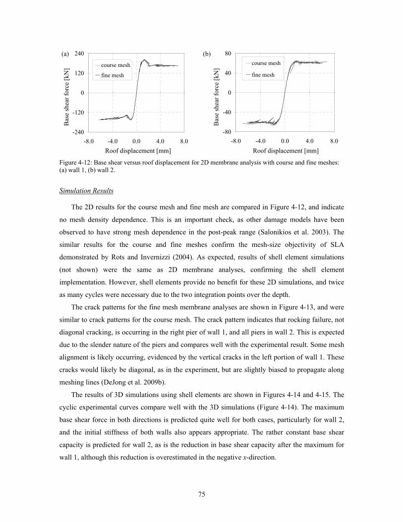
75

Figure 4-12: Base shear versus roof displacement for 2D membrane analysis with course and fine meshes: (a) wall 1, (b) wall 2.

Simulation Results

The 2D results for the course mesh and fine mesh are compared in Figure 4-12, and indicate

no mesh density dependence. This is an important check, as other damage models have been

observed to have strong mesh dependence in the post-peak range (Salonikios et al. 2003). The

similar results for the course and fine meshes confirm the mesh-size objectivity of SLA

demonstrated by Rots and Invernizzi (2004). As expected, results of shell element simulations

(not shown) were the same as 2D membrane analyses, confirming the shell element

implementation. However, shell elements provide no benefit for these 2D simulations, and twice

as many cycles were necessary due to the two integration points over the depth.

The crack patterns for the fine mesh membrane analyses are shown in Figure 4-13, and were

similar to crack patterns for the course mesh. The crack pattern indicates that rocking failure, not

diagonal cracking, is occurring in the right pier of wall 1, and all piers in wall 2. This is expected

due to the slender nature of the piers and compares well with the experimental result. Some mesh

alignment is likely occurring, evidenced by the vertical cracks in the left portion of wall 1. These

cracks would likely be diagonal, as in the experiment, but are slightly biased to propagate along

meshing lines (DeJong et al. 2009b).

The results of 3D simulations using shell elements are shown in Figures 4-14 and 4-15. The

cyclic experimental curves compare well with the 3D simulations (Figure 4-14). The maximum

base shear force in both directions is predicted quite well for both cases, particularly for wall 2,

and the initial stiffness of both walls also appears appropriate. The rather constant base shear

capacity is predicted for wall 2, as is the reduction in base shear capacity after the maximum for

wall 1, although this reduction is overestimated in the negative x-direction.

-240

-120

0

120

240

-8.0 -4.0 0.0 4.0 8.0

course mesh

fine meshB

ase

shea

r for

ce [k

N]

(b)(a)

-80

-40

0

40

80

-8.0 -4.0 0.0 4.0 8.0

course mesh

fine mesh

Roof displacement [mm]

Bas

e sh

ear f

orce

[kN

]


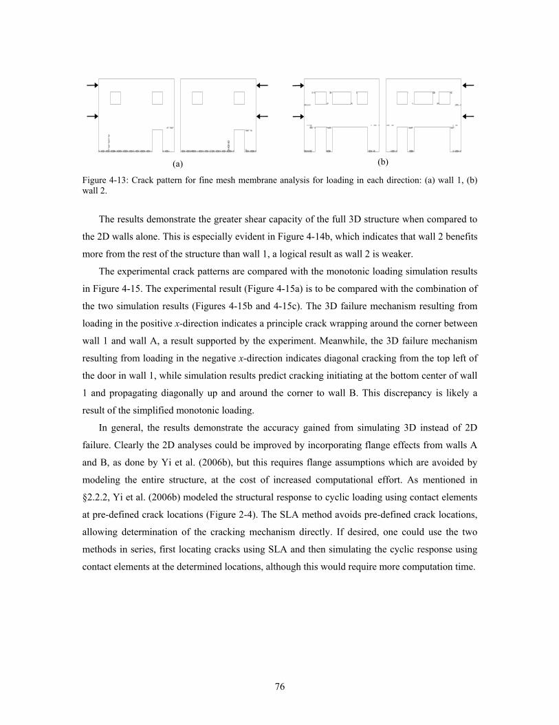
76

Figure 4-13: Crack pattern for fine mesh membrane analysis for loading in each direction: (a) wall 1, (b) wall 2.

The results demonstrate the greater shear capacity of the full 3D structure when compared to

the 2D walls alone. This is especially evident in Figure 4-14b, which indicates that wall 2 benefits

more from the rest of the structure than wall 1, a logical result as wall 2 is weaker.

The experimental crack patterns are compared with the monotonic loading simulation results

in Figure 4-15. The experimental result (Figure 4-15a) is to be compared with the combination of

the two simulation results (Figures 4-15b and 4-15c). The 3D failure mechanism resulting from

loading in the positive x-direction indicates a principle crack wrapping around the corner between

wall 1 and wall A, a result supported by the experiment. Meanwhile, the 3D failure mechanism

resulting from loading in the negative x-direction indicates diagonal cracking from the top left of

the door in wall 1, while simulation results predict cracking initiating at the bottom center of wall

1 and propagating diagonally up and around the corner to wall B. This discrepancy is likely a

result of the simplified monotonic loading.

In general, the results demonstrate the accuracy gained from simulating 3D instead of 2D

failure. Clearly the 2D analyses could be improved by incorporating flange effects from walls A

and B, as done by Yi et al. (2006b), but this requires flange assumptions which are avoided by

modeling the entire structure, at the cost of increased computational effort. As mentioned in

§2.2.2, Yi et al. (2006b) modeled the structural response to cyclic loading using contact elements

at pre-defined crack locations (Figure 2-4). The SLA method avoids pre-defined crack locations,

allowing determination of the cracking mechanism directly. If desired, one could use the two

methods in series, first locating cracks using SLA and then simulating the cyclic response using

contact elements at the determined locations, although this would require more computation time.

(a) (b)

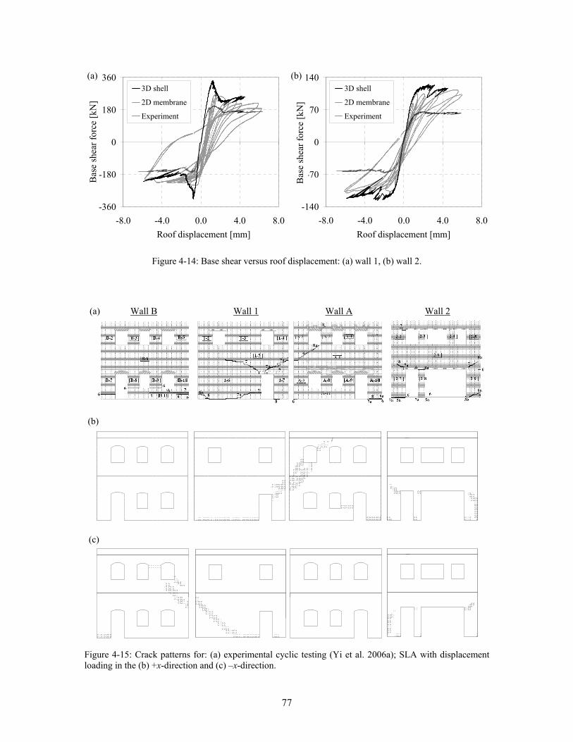
77

Figure 4-14: Base shear versus roof displacement: (a) wall 1, (b) wall 2.

Figure 4-15: Crack patterns for: (a) experimental cyclic testing (Yi et al. 2006a); SLA with displacement loading in the (b) +x-direction and (c) –x-direction.

(c)

(b)

(a) Wall B Wall 1 Wall A Wall 2

-140

-70

0

70

140

-8.0 -4.0 0.0 4.0 8.0

3D shell

2D membrane

Experiment

-360

-180

0

180

360

-8.0 -4.0 0.0 4.0 8.0

3D shell

2D membrane

Experiment

(b)


Bas

e sh

ear f

orce

[kN

]

(a)


Bas

e sh

ear f

orce

[kN

]

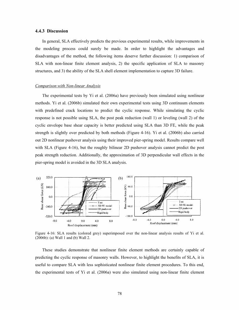
78

4.4.3 Discussion

In general, SLA effectively predicts the previous experimental results, while improvements in

the modeling process could surely be made. In order to highlight the advantages and

disadvantages of the method, the following items deserve further discussion: 1) comparison of

SLA with non-linear finite element analysis, 2) the specific application of SLA to masonry

structures, and 3) the ability of the SLA shell element implementation to capture 3D failure.

Comparison with Non-linear Analysis

The experimental tests by Yi et al. (2006a) have previously been simulated using nonlinear

methods. Yi et al. (2006b) simulated their own experimental tests using 3D continuum elements

with predefined crack locations to predict the cyclic response. While simulating the cyclic

response is not possible using SLA, the post peak reduction (wall 1) or leveling (wall 2) of the

cyclic envelope base shear capacity is better predicted using SLA than 3D FE, while the peak

strength is slightly over predicted by both methods (Figure 4-16). Yi et al. (2006b) also carried

out 2D nonlinear pushover analysis using their improved pier-spring model. Results compare well

with SLA (Figure 4-16), but the roughly bilinear 2D pushover analysis cannot predict the post

peak strength reduction. Additionally, the approximation of 3D perpendicular wall effects in the

pier-spring model is avoided in the 3D SLA analysis.

Figure 4-16: SLA results (colored grey) superimposed over the non-linear analysis results of Yi et al. (2006b): (a) Wall 1 and (b) Wall 2.

These studies demonstrate that nonlinear finite element methods are certainly capable of

predicting the cyclic response of masonry walls. However, to highlight the benefits of SLA, it is

useful to compare SLA with less sophisticated nonlinear finite element procedures. To this end,

the experimental tests of Yi et al. (2006a) were also simulated using non-linear finite element

(b)(a)

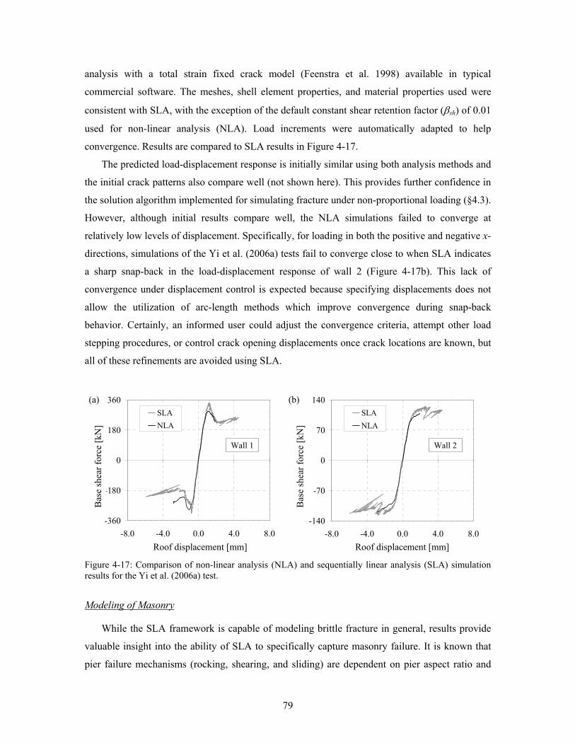
79

analysis with a total strain fixed crack model (Feenstra et al. 1998) available in typical

commercial software. The meshes, shell element properties, and material properties used were

consistent with SLA, with the exception of the default constant shear retention factor (βsh) of 0.01

used for non-linear analysis (NLA). Load increments were automatically adapted to help

convergence. Results are compared to SLA results in Figure 4-17.

The predicted load-displacement response is initially similar using both analysis methods and

the initial crack patterns also compare well (not shown here). This provides further confidence in

the solution algorithm implemented for simulating fracture under non-proportional loading (§4.3).

However, although initial results compare well, the NLA simulations failed to converge at

relatively low levels of displacement. Specifically, for loading in both the positive and negative x-

directions, simulations of the Yi et al. (2006a) tests fail to converge close to when SLA indicates

a sharp snap-back in the load-displacement response of wall 2 (Figure 4-17b). This lack of

convergence under displacement control is expected because specifying displacements does not

allow the utilization of arc-length methods which improve convergence during snap-back

behavior. Certainly, an informed user could adjust the convergence criteria, attempt other load

stepping procedures, or control crack opening displacements once crack locations are known, but

all of these refinements are avoided using SLA.

Figure 4-17: Comparison of non-linear analysis (NLA) and sequentially linear analysis (SLA) simulation results for the Yi et al. (2006a) test.

Modeling of Masonry

While the SLA framework is capable of modeling brittle fracture in general, results provide

valuable insight into the ability of SLA to specifically capture masonry failure. It is known that

pier failure mechanisms (rocking, shearing, and sliding) are dependent on pier aspect ratio and

-140

-70

0

70

140

-8.0 -4.0 0.0 4.0 8.0

SLANLA

-360

-180

0

180

360

-8.0 -4.0 0.0 4.0 8.0

SLANLA

Wall 1


Bas

e sh

ear f

orce

[kN

]

(a) (b)

Wall 2


Bas

e sh

ear f

orce

[kN

]

80

axial load (Calvi et al. 1996). In §4.4.2, the building tested by Yi et al. (2006a) was subjected to

low vertical loads (only self-weight) resulting in low axial loads in the piers. As a result, failure

of wall 2 occurred through rocking of the slender piers (Yi 2004), and failure of wall 1 occurred

through initial rocking followed by sliding of the stout, left pier. Shear failure in the piers, which

typically occurs due to high axial loads (Calvi et al. 1996), was not observed. In contrast, SLA

simulations of buildings subjected to large vertical loads resulted primarily in shear failure,

followed by significant sliding failure (DeJong et al. 2009a).

In general, rocking failure is well predicted using SLA but the base shear tends to be

overestimated when shear failure occurs (DeJong et al. 2009a). One primary reason for this is

likely that a biaxial failure envelope for masonry has not been considered. The shear failure

which occurs in the piers results from tensile stresses in the primary principle stress direction and

compressive stresses in the secondary principle stress direction, which is currently neglected.

When these secondary compressive stresses are large, a biaxial failure envelope would result in a

reduction in the allowable tensile strength, and therefore a reduction in the base shear capacity.

It should also be noted that the failure mode, shear or rocking, is dependent on the material

tensile strength, which is difficult to estimate. A larger tensile strength would cause a larger

increase in shear capacity than rocking capacity. Therefore, a larger vertical tensile strength has a

similar effect on the failure mode as a lower axial load. This effect was observed in other

simulations of masonry failure using SLA for shell pushover studies (DeJong et al. 2009a), as

doubling the tensile strength resulted in increased rocking failure and decreased diagonal pier

cracking.

Finally, simulation results indicate that while rocking failure and shear failure can both be

predicted using SLA, accuracy could be improved through a material model which incorporates

the heterogeneous nature of masonry. However, large displacement sliding failure cannot be

modeled at this point. If significant sliding failure is expected based on wall geometries and axial

loads (Calvi et al. 1996), then care should be taken when using this model.

Three-dimensional Failure Mechanisms

In §4.4.2, the shell element implementation was shown to predict 3D failure mechanisms in

which cracks propagate around building corners. This contribution is significant, as prediction of

the failure mechanisms is achieved with a simple material model which requires relatively few

material properties and no load stepping procedures or convergence criteria.

Simulation results exemplify the greater capacity of the entire structure with respect to a

single wall. Clearly some effect of perpendicular walls must be included, and the 3D models

81

eliminate the need to estimate 3D wall corners effects. The simulated 3D capacity of the Yi et al.

(2006a) structure is quite accurate, while the 2D membrane element models clearly underestimate

the response (Figure 4-14).

4.5 Summary

The primary contributions herein are the extension of SLA to incorporate non-proportional

loading, and the new framework by which shell structures can be effectively modeled under non-

proportional loading. Application to a masonry structure under quasi-static lateral loading, a

simplification of expected earthquake loading, has led to the following specific conclusions:

• SLA effectively predicts damage due to the brittle material failure of masonry, and

requires a relatively small number of modeling parameters.

• Shell elements allow three dimensional collapse mechanisms to be directly predicted,

eliminating the need to estimate the participating area of perpendicular walls when

modeling in two dimensions.

• Monotonic loading provides an effective means of predicting experimental cyclic

envelopes, although can result in slight overestimation of the maximum base shear. A

safety factor should be applied to account for the simplified loading conditions.

• The simplified uni-axial tensile strength failure criterion reasonably predicts structural

response. However, implementation of a more complex failure criterion which

incorporates the heterogeneity of masonry is possible within the same framework.

In addition to these specific conclusions, the benefit of this improved brittle fracture

modeling method must be reiterated within the context of this dissertation. The primary

advantage of SLA when compared to equilibrium methods (e.g. Chapter 3) is its ability to model

damage. The advantage of SLA when compared to other finite element brittle fracture models is

its ability to model continued damage without convergence issues, thus being able to predict a

greater extent of damage. Therefore, SLA provides a new useful tool for explaining existing crack

patterns and predicting where damage might be expected during future earthquakes. Additionally,

improved damage predictions can be used to better define possible collapse mechanisms.

Predicted collapse mechanisms could then be used to inform quasi-static equilibrium analyses.

Furthermore, while modeling the dynamic response of the structure is not possible using SLA,

defined collapse mechanisms could also be used to inform dynamic analyses using the

approaches discussed in Part III of this dissertation.

83

Part III

Dynamic Analysis

84

Chapter 5

Analytical Modeling: Dynamics of Arches

5.1 Introduction

Part III narrows the scope to dynamic assessment methods for masonry structures focused on

stability, not strength. In effect, this means concentrating on the dynamics of discrete block

structures. The majority of attention is paid to relatively simple structures, or structural

components, whose dynamic behavior must be understood before using numerical tools to assess

more complex structures.

Despite the prevalence of the masonry arch, its dynamic behavior under seismic loading has

not been well-described. Therefore, a better understanding of the response of masonry arches

(and vaults) to dynamic loading is necessary to develop tools which can be used to assess the

safety of these structures.

In this chapter, an analytical model for the dynamics of masonry arches is first presented in

§5.2 and the limitations of the model are discussed. Subsequently, in §5.3 an experimental

program is presented which tests the stability of masonry arches under harmonic and seismic

ground motion. Experimental results are compared with predictions from the analytical model. In

§5.4, the analytical model is used to make steps towards a criterion for evaluating the safety of

masonry arches in seismic regions. Although other assessment procedures have been developed

(e.g. De Luca et al. 2004), they have been based on static analyses which do not incorporate the

dynamics of the problem. Finally, results and conclusions are summarized in §5.5.

85

5.2 An Analytical Arch Model

As discussed in §2.3.1, Oppenheim (1992) developed an analytical model which describes the

arch as a rigid body four-link mechanism and predicts failure of the arch in response to a given

base impulse excitation. Although Oppenheim did not address the problem of what occurs if the

arch recovers from the single impulse and ‘rocks’ in the other direction, his analytical model

effectively poses the problem as a ‘rocking arch’ which is similar to the rocking block. Since

these two systems are similar, the fundamental work on the rocking block (Housner 1963, see

§2.3.1) will be used to guide the derivations herein.

The analytical model presented in this section builds upon the work by Oppenheim (1992) by

addressing the impact which occurs if the arch recovers, and can therefore describe the motion of

the arch through continued rocking cycles. Similar to rocking block models, the rocking arch

model assumes rigid blocks and rigid supports and is therefore only dependent on geometric

properties. For more details regarding the analytical model and its implementation in Matlab

(2002), see De Lorenzis et al. (2007) and Appendix B. The model and the included impact

formulation is a simplification of the actual response of the masonry arch under dynamic loading,

but this chapter will attempt to illuminate the utility of such a model.

5.2.1 The Arch as a Four-hinge Mechanism

Following the work by Oppenheim (1992), the part-circular arch with center-line radius RA,

thickness tA, and angle of embrace βA, is modeled as a four-hinge mechanism. The four hinges

which create the three-bar mechanism ABCD (Figure 5-1a) are assumed to form at the locations

where they would form under equivalent static analysis, i.e. under a ‘tilt test’ where the base is

quasi-statically tilted until collapse occurs (see Chapter 3). The minimum tilt angle at which

collapse occurs in the quasi-static test correlates to the theoretical minimum base acceleration, γ ,

which would cause the four-link mechanism to form. (The arch would collapse if this horizontal

base acceleration were applied for an infinite length of time.) The problem is purely geometrical;

γ is a function of tA , RA , βA, and the number of voussoirs, nA.

The assumed single degree of freedom (SDOF) mechanism allows the response of the arch to

a given ground acceleration, ( )gu t , to be described by the following equation of motion which

can be derived using Hamilton’s principle and Lagrange’s equation:

( ) ( ) ( ) ( )2+ + =A A gM R L R F g P uθ θ θ θ θ θ (5.1)

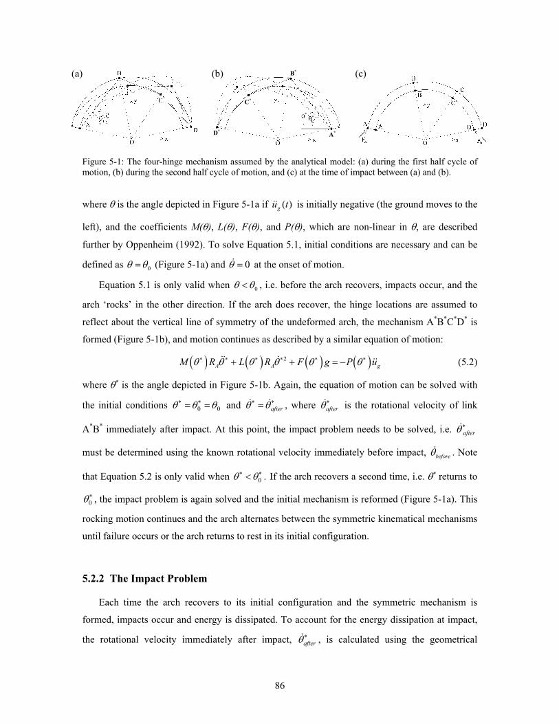
86

Figure 5-1: The four-hinge mechanism assumed by the analytical model: (a) during the first half cycle of motion, (b) during the second half cycle of motion, and (c) at the time of impact between (a) and (b).

where θ is the angle depicted in Figure 5-1a if ( )gu t is initially negative (the ground moves to the

left), and the coefficients M(θ), L(θ), F(θ), and P(θ), which are non-linear in θ, are described

further by Oppenheim (1992). To solve Equation 5.1, initial conditions are necessary and can be

defined as 0=θ θ (Figure 5-1a) and 0=θ at the onset of motion.

Equation 5.1 is only valid when 0<θ θ , i.e. before the arch recovers, impacts occur, and the

arch ‘rocks’ in the other direction. If the arch does recover, the hinge locations are assumed to

reflect about the vertical line of symmetry of the undeformed arch, the mechanism A*B*C*D* is

formed (Figure 5-1b), and motion continues as described by a similar equation of motion:

( ) ( ) ( ) ( )2∗ ∗ ∗ ∗ ∗ ∗+ + = −A A gM R L R F g P uθ θ θ θ θ θ (5.2)

where θ∗ is the angle depicted in Figure 5-1b. Again, the equation of motion can be solved with

the initial conditions 0 0∗ ∗= =θ θ θ and ∗ ∗= afterθ θ , where ∗

afterθ is the rotational velocity of link

A*B* immediately after impact. At this point, the impact problem needs to be solved, i.e. ∗afterθ

must be determined using the known rotational velocity immediately before impact, beforeθ . Note

that Equation 5.2 is only valid when 0∗ ∗<θ θ . If the arch recovers a second time, i.e. θ∗ returns to

0∗θ , the impact problem is again solved and the initial mechanism is reformed (Figure 5-1a). This

rocking motion continues and the arch alternates between the symmetric kinematical mechanisms

until failure occurs or the arch returns to rest in its initial configuration.

5.2.2 The Impact Problem

Each time the arch recovers to its initial configuration and the symmetric mechanism is

formed, impacts occur and energy is dissipated. To account for the energy dissipation at impact,

the rotational velocity immediately after impact, ∗afterθ , is calculated using the geometrical

A*

B*

C*

D*

**

(b) (a) (c)

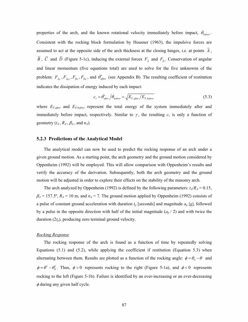
87

properties of the arch, and the known rotational velocity immediately before impact, beforeθ .

Consistent with the rocking block formulation by Housner (1963), the impulsive forces are

assumed to act at the opposite side of the arch thickness at the closing hinges, i.e. at points A ,

B , C and D (Figure 5-1c), inducing the external forces AF and DF . Conservation of angular

and linear momentum (five equations total) are used to solve for the five unknowns of the

problem: AxF , AxyF , DxF , DyF , and ∗afterθ (see Appendix B). The resulting coefficient of restitution

indicates the dissipation of energy induced by each impact:

, ,∗= =v after before T after T beforec E Eθ θ (5.3)

where ET,after and ET,before represent the total energy of the system immediately after and

immediately before impact, respectively. Similar to γ , the resulting cv is only a function of

geometry (tA , RA , βA , and nA).

5.2.3 Predictions of the Analytical Model

The analytical model can now be used to predict the rocking response of an arch under a

given ground motion. As a starting point, the arch geometry and the ground motion considered by

Oppenheim (1992) will be employed. This will allow comparison with Oppenheim’s results and

verify the accuracy of the derivation. Subsequently, both the arch geometry and the ground

motion will be adjusted in order to explore their effects on the stability of the masonry arch.

The arch analyzed by Oppenheim (1992) is defined by the following parameters: tA/RA = 0.15,

βA = 157.5º, RA = 10 m, and nA = 7. The ground motion applied by Oppenheim (1992) consists of

a pulse of constant ground acceleration with duration tp [seconds] and magnitude ap [g], followed

by a pulse in the opposite direction with half of the initial magnitude (ap / 2) and with twice the

duration (2tp), producing zero terminal ground velocity.

Rocking Response

The rocking response of the arch is found as a function of time by repeatedly solving

Equations (5.1) and (5.2), while applying the coefficient if restitution (Equation 5.3) when

alternating between them. Results are plotted as a function of the rocking angle: 0= −φ θ θ and

0∗ ∗= −φ θ θ . Thus, 0>φ represents rocking to the right (Figure 5-1a), and 0<φ represents

rocking to the left (Figure 5-1b). Failure is identified by an ever-increasing or an ever-decreasing

φ during any given half cycle.

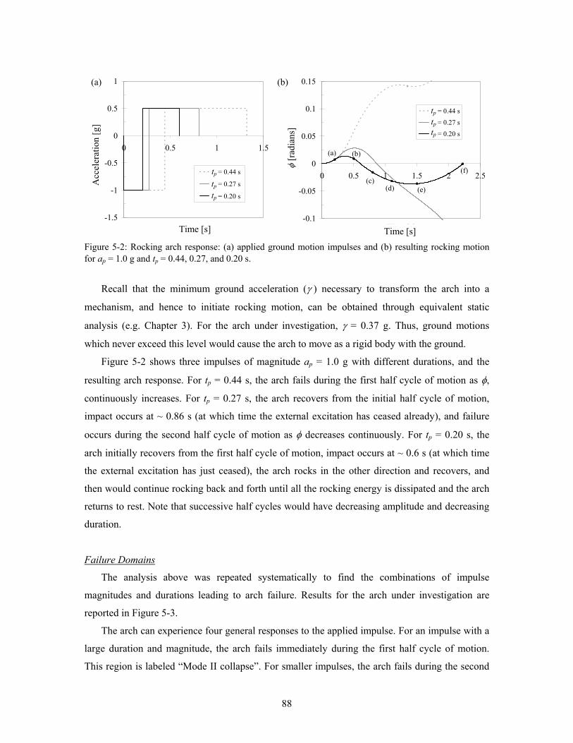
88

Figure 5-2: Rocking arch response: (a) applied ground motion impulses and (b) resulting rocking motion for ap = 1.0 g and tp = 0.44, 0.27, and 0.20 s.

Recall that the minimum ground acceleration (γ ) necessary to transform the arch into a

mechanism, and hence to initiate rocking motion, can be obtained through equivalent static

analysis (e.g. Chapter 3). For the arch under investigation, γ = 0.37 g. Thus, ground motions

which never exceed this level would cause the arch to move as a rigid body with the ground.

Figure 5-2 shows three impulses of magnitude ap = 1.0 g with different durations, and the

resulting arch response. For tp = 0.44 s, the arch fails during the first half cycle of motion as φ,

continuously increases. For tp = 0.27 s, the arch recovers from the initial half cycle of motion,

impact occurs at ~ 0.86 s (at which time the external excitation has ceased already), and failure

occurs during the second half cycle of motion as φ decreases continuously. For tp = 0.20 s, the

arch initially recovers from the first half cycle of motion, impact occurs at ~ 0.6 s (at which time

the external excitation has just ceased), the arch rocks in the other direction and recovers, and

then would continue rocking back and forth until all the rocking energy is dissipated and the arch

returns to rest. Note that successive half cycles would have decreasing amplitude and decreasing

duration.

Failure Domains

The analysis above was repeated systematically to find the combinations of impulse

magnitudes and durations leading to arch failure. Results for the arch under investigation are

reported in Figure 5-3.

The arch can experience four general responses to the applied impulse. For an impulse with a

large duration and magnitude, the arch fails immediately during the first half cycle of motion.

This region is labeled “Mode II collapse”. For smaller impulses, the arch fails during the second

-0.1

-0.05

0

0.05

0.1

0.15

0 0.5 1 1.5 2 2.5

Time [s]

φ [

radi

ans]

tp = 0.44 s

tp = 0.27 s

tp = 0.20 s

tp tp tp

(b)(a)

(c)(d) (e)

(f)

Time [s]

(a) (b)

-1.5

-1

-0.5

0

0.5

1

0 0.5 1 1.5

Time [s]

Acc

eler

atio

n [g

]

tp = 0.44 s

tp = 0.27 s

tp = 0.20 s

tp tp tp

φ [r

adia

ns]

Time [s]

Acc

eler

atio

n [g

]

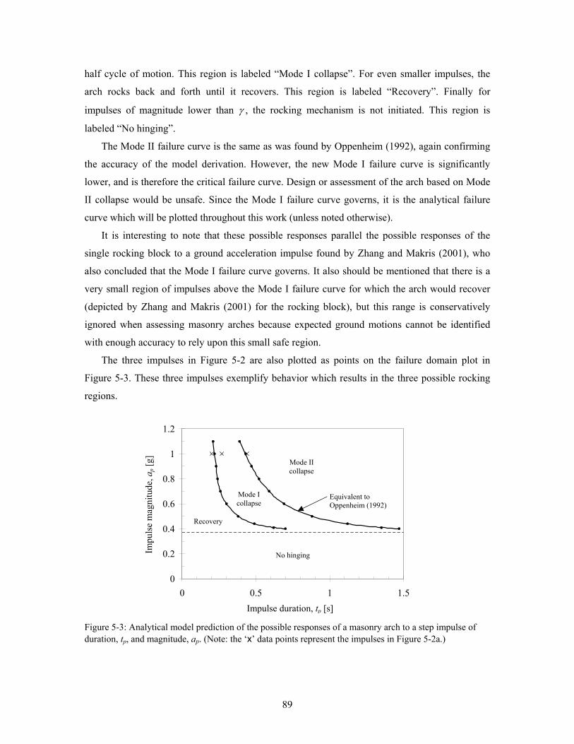
89

half cycle of motion. This region is labeled “Mode I collapse”. For even smaller impulses, the

arch rocks back and forth until it recovers. This region is labeled “Recovery”. Finally for

impulses of magnitude lower than γ , the rocking mechanism is not initiated. This region is

labeled “No hinging”.

The Mode II failure curve is the same as was found by Oppenheim (1992), again confirming

the accuracy of the model derivation. However, the new Mode I failure curve is significantly

lower, and is therefore the critical failure curve. Design or assessment of the arch based on Mode

II collapse would be unsafe. Since the Mode I failure curve governs, it is the analytical failure

curve which will be plotted throughout this work (unless noted otherwise).

It is interesting to note that these possible responses parallel the possible responses of the

single rocking block to a ground acceleration impulse found by Zhang and Makris (2001), who

also concluded that the Mode I failure curve governs. It also should be mentioned that there is a

very small region of impulses above the Mode I failure curve for which the arch would recover

(depicted by Zhang and Makris (2001) for the rocking block), but this range is conservatively

ignored when assessing masonry arches because expected ground motions cannot be identified

with enough accuracy to rely upon this small safe region.

The three impulses in Figure 5-2 are also plotted as points on the failure domain plot in

Figure 5-3. These three impulses exemplify behavior which results in the three possible rocking

regions.

Figure 5-3: Analytical model prediction of the possible responses of a masonry arch to a step impulse of duration, tp, and magnitude, ap. (Note: the ‘x’ data points represent the impulses in Figure 5-2a.)

0

0.2

0.4

0.6

0.8

1

1.2

0 0.5 1 1.5

Impulse duration, t d [s]

Impu

lse

mag

nitu

de, a

[g]

Equivalent to Oppenheim (1992)

Mode I collapse

Mode IIcollapse

Recovery

No hinging

Impulse duration, tp [s]

Impu

lse

mag

nitu

de, a

p [g]

90

Figure 5-4: Analytical model predictions of the failure curves for masonry arches of different radii (RA) but of the same proportions (tA/RA = 0.15 and βA = 157.5º).

Scale Effect

The presence of the arch radius R in the differential equations of motion implies the existence

of a scale effect, i.e. arches with the same proportions (tA/RA , βA) but different sizes will have

different dynamic response. This scale effect is illustrated in Figure 5-4, which shows the Mode I

failure curves for similar arches (tA/RA = 0.15 and βA = 157.5º) with different radii. The RA = 10 m

arch was analyzed in the previous section.

Figure 5-4 demonstrates that larger arches are clearly more stable than smaller ones with the

same proportions. Furthermore, the failure domain curves are approximately scalable with the

square root of the radius. For example, if one of the failure curves is taken as reference and the

impulse magnitude corresponding to a given tp is multiplied by the square root of the ratio of any

desired radius RA to the reference radius, the other failure domain curves are obtained. Thus, it is

only necessary to compute rigorously the failure domain for an arbitrary reference radius. This

confirms the findings of Housner (1963), and is explored further in §5.4.

Effect of Arch Geometry

Figure 5-5 illustrates the effect of the arch geometry, in terms of tA/RA and βA, on the arch

failure domains. As expected, increasing the tA/RA ratio and decreasing the angle of inclusion (βA)

increases the resistance of the arch to impulse ground motion, i.e. increasing its stability. These

geometric changes also result in the assumption of slightly different four-hinge mechanisms (see

Figure 5-5), which explains why the failure domains are not evenly distributed.

0

0.2

0.4

0.6

0.8

1

1.2

0 0.5 1 1.5 2Impulse duration, t d [s]

Impu

lse

mag

nitu

de, a

[g]

1 m5 m10 m20 m


Impu

lse

mag

nitu

de, a

p [g]

91

Figure 5-5: Analytical model predictions of the failure curves for masonry arches of the same radius (RA = 10 m) but of different proportions (tA / RA and βA).

The uneven distribution visible in Figure 5-5, suggests that the number of voussiors has an

effect on the failure domains. More voussoirs would make the shift in mechanisms less drastic,

and therefore the spacing of the failure curves would be more even. Thus, the effect of a greater

number of voussoirs on the magnitude-duration failure domain was also investigated. As

expected, increasing the number of voussoirs was found to effectively increase the resolution of

the possible initial hinge locations which are found using equivalent static analysis. While this

does change the four-link mechanism, it has a relatively small effect on the failure domains

compared to a change in tA/RA or βA.

0

0.2

0.4

0.6

0.8

1

1.2

0 0.2 0.4 0.6 0.8 1Impulse duration, t d [s]

Impu

lse

mag

nitu

de, a

[g]

tA / RA = 0.11 tA / RA = 0.15 tA / RA = 0.17 tA / RA = 0.19

0

0.2

0.4

0.6

0.8

1

1.2

0 0.2 0.4 0.6 0.8 1Impulse duration, t d [s]

Impu

lse

mag

nitu

de, a

[g]

β = 165

β = 157.5

β = 150

β = 142.5

A

A

A

A

symmetric mechanism

asymmetric mechanism

symmetric mechanism

asymmetric mechanism


Impu

lse

mag

nitu

de, a

p [g]


Impu

lse

mag

nitu

de, a

p [g]

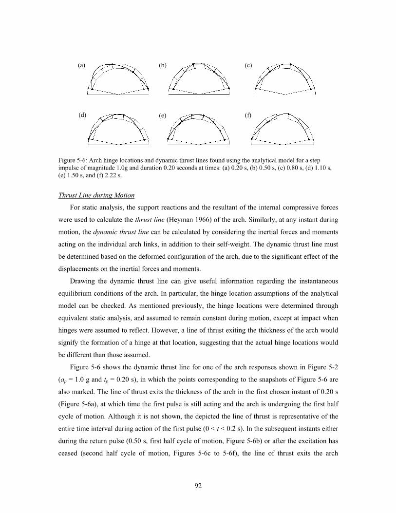
92

Figure 5-6: Arch hinge locations and dynamic thrust lines found using the analytical model for a step impulse of magnitude 1.0g and duration 0.20 seconds at times: (a) 0.20 s, (b) 0.50 s, (c) 0.80 s, (d) 1.10 s, (e) 1.50 s, and (f) 2.22 s.

Thrust Line during Motion

For static analysis, the support reactions and the resultant of the internal compressive forces

were used to calculate the thrust line (Heyman 1966) of the arch. Similarly, at any instant during

motion, the dynamic thrust line can be calculated by considering the inertial forces and moments

acting on the individual arch links, in addition to their self-weight. The dynamic thrust line must

be determined based on the deformed configuration of the arch, due to the significant effect of the

displacements on the inertial forces and moments.

Drawing the dynamic thrust line can give useful information regarding the instantaneous

equilibrium conditions of the arch. In particular, the hinge location assumptions of the analytical

model can be checked. As mentioned previously, the hinge locations were determined through

equivalent static analysis, and assumed to remain constant during motion, except at impact when

hinges were assumed to reflect. However, a line of thrust exiting the thickness of the arch would

signify the formation of a hinge at that location, suggesting that the actual hinge locations would

be different than those assumed.

Figure 5-6 shows the dynamic thrust line for one of the arch responses shown in Figure 5-2

(ap = 1.0 g and tp = 0.20 s), in which the points corresponding to the snapshots of Figure 5-6 are

also marked. The line of thrust exits the thickness of the arch in the first chosen instant of 0.20 s

(Figure 5-6a), at which time the first pulse is still acting and the arch is undergoing the first half

cycle of motion. Although it is not shown, the depicted the line of thrust is representative of the

entire time interval during action of the first pulse (0 < t < 0.2 s). In the subsequent instants either

during the return pulse (0.50 s, first half cycle of motion, Figure 5-6b) or after the excitation has

ceased (second half cycle of motion, Figures 5-6c to 5-6f), the line of thrust exits the arch

(a) (b) (c)

(d) (e) (f)

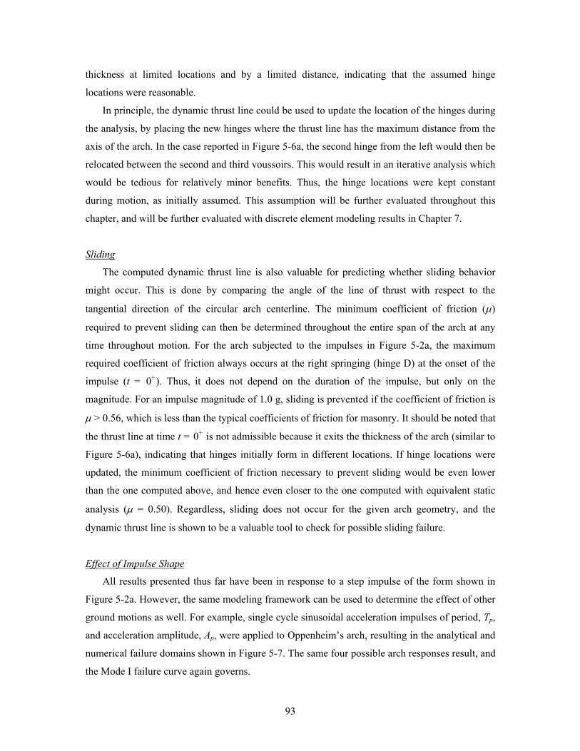
93

thickness at limited locations and by a limited distance, indicating that the assumed hinge

locations were reasonable.

In principle, the dynamic thrust line could be used to update the location of the hinges during

the analysis, by placing the new hinges where the thrust line has the maximum distance from the

axis of the arch. In the case reported in Figure 5-6a, the second hinge from the left would then be

relocated between the second and third voussoirs. This would result in an iterative analysis which

would be tedious for relatively minor benefits. Thus, the hinge locations were kept constant

during motion, as initially assumed. This assumption will be further evaluated throughout this

chapter, and will be further evaluated with discrete element modeling results in Chapter 7.

Sliding

The computed dynamic thrust line is also valuable for predicting whether sliding behavior

might occur. This is done by comparing the angle of the line of thrust with respect to the

tangential direction of the circular arch centerline. The minimum coefficient of friction (μ)

required to prevent sliding can then be determined throughout the entire span of the arch at any

time throughout motion. For the arch subjected to the impulses in Figure 5-2a, the maximum

required coefficient of friction always occurs at the right springing (hinge D) at the onset of the

impulse (t = 0+). Thus, it does not depend on the duration of the impulse, but only on the

magnitude. For an impulse magnitude of 1.0 g, sliding is prevented if the coefficient of friction is

μ > 0.56, which is less than the typical coefficients of friction for masonry. It should be noted that

the thrust line at time t = 0+ is not admissible because it exits the thickness of the arch (similar to

Figure 5-6a), indicating that hinges initially form in different locations. If hinge locations were

updated, the minimum coefficient of friction necessary to prevent sliding would be even lower

than the one computed above, and hence even closer to the one computed with equivalent static

analysis (μ = 0.50). Regardless, sliding does not occur for the given arch geometry, and the

dynamic thrust line is shown to be a valuable tool to check for possible sliding failure.

Effect of Impulse Shape

All results presented thus far have been in response to a step impulse of the form shown in

Figure 5-2a. However, the same modeling framework can be used to determine the effect of other

ground motions as well. For example, single cycle sinusoidal acceleration impulses of period, Tp,

and acceleration amplitude, Ap, were applied to Oppenheim’s arch, resulting in the analytical and

numerical failure domains shown in Figure 5-7. The same four possible arch responses result, and

the Mode I failure curve again governs.

94

Figure 5-7: Failure domains of Oppenheim’s arch in response to a single cycle sinusoidal impulse function of period, Tp, and amplitude, Ap.

5.3 Experimental Investigation of Arch Dynamics

This section is focused on an experimental investigation designed to obtain a better

fundamental understanding of masonry arch dynamics, and to evaluate the analytical model

presented in §5.2. Before the rigorous experimental results are presented, qualitative observations

are described and used to evaluate the assumptions of the analytical model.

5.3.1 Evaluation of Analytical Model Assumptions

The assumptions included in the analytical model clearly lead to some limitations. First, the

assumption of fixed hinge locations does not allow: (1) free initial hinge formation, (2) free hinge

formation after impact, (3) opening at any non-hinged joint, or (4) sliding between blocks.

Second, the assumption of rigid blocks does not allow elastic deformation, meaning that

resonance cannot be modeled, and does not allow material failure during impact. Third, the

assumption of perfectly rigid supports does not allow for support deformation which could reduce

stability.

Although some of these limitations were discussed in §5.2.2, experimental tests were used to

address them more completely. To this end, small scale arches were subjected to both a harmonic

base motion with linearly increasing amplitude and a variety of earthquake time histories, and

behavior was observed. The response of an arch made of aerated concrete blocks with a center-

line radius of 15 cm and with 13 voussoirs is shown in Figures 5-8 and 5-9. Under harmonic base

0

0.2

0.4

0.6

0.8

1

1.2

0 1 2 3 4 5Impulse period, T p [s]

Impu

lse

ampl

itude

, Ap

[g]

Mode I collapse

Mode IIcollapse

Recovery

No hinging

Impulse period, Tp [s]

Impu

lse

ampl

itude

, Ap [

g]

95

motion, the arch initially moved as a rigid body with the base, with only minor vibration and no

visible hinge mechanisms. As the amplitude increased, slight hinging occurred as the arch rocked

back and forth. More visible hinging occurred in the final two rocking mechanisms which are

shown in Figure 5-8. Under the El Centro earthquake time history in Figure 5-9a, four primary

rocking mechanisms were formed before collapse (Figures 5-9b,c,d,e). The four corresponding

rocking mechanisms predicted by the analytical model are also shown in Figure 5-9. The first two

rocking mechanisms are less visible and result from the first smaller acceleration peaks in Figure

5-9a. The final mechanism (Figure 3e), which resulted in collapse, is induced by the first large

negative peak and the large positive peak (the largest one) which immediately follows.

In Figures 5-8 and 5-9, the consecutive hinge mechanisms are shown at their maximum

magnitude, and indicate that a four-hinge mechanism does form and that the hinges do

approximately reflect. However, hinge mechanisms are not always exactly symmetric and the

transition between these mechanisms does not occur in one distinct impact. In fact, hinge

reflection is more fluent as hinges seem to ‘migrate’ instead of reflecting directly. Sliding was not

observed, confirming the predictions of dynamic thrust line analysis presented in §5.2.2.

These observations indicate that through the first assumption mentioned above, that of fixed

hinges, the analytical model describes a reasonable simplification of behavior. The second

assumption, that of rigid blocks, is appropriate for the scale tested because negligible material

failure occurred and the elastic resonant frequency of the first mode of the arch tested is over 300

Hz, well above the frequency content of the earthquake. However, the effects of the rigid block

assumption are scale dependent. At larger scales, larger impact forces could cause material

failure, especially at block corners, and the resonant frequency would be lower and could be

excited. Regardless, it must be noted that resonance could only force hinges to occur at a lower

acceleration than expected; resonance could not amplify the response until collapse because

initial hinge formation immediately changes the resonant frequency. The third limitation, that of

rigid supports, remains and is the subject of continued research.

Based on these observations, a more complete experimental investigation was conducted to

test the ability of the analytical model to predict the collapse of arches under seismic loading.

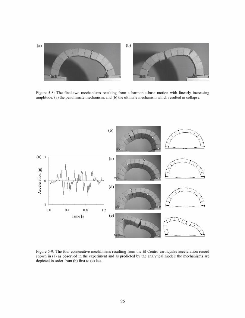
96

Figure 5-8: The final two mechanisms resulting from a harmonic base motion with linearly increasing amplitude: (a) the penultimate mechanism, and (b) the ultimate mechanism which resulted in collapse.

Figure 5-9: The four consecutive mechanisms resulting from the El Centro earthquake acceleration record shown in (a) as observed in the experiment and as predicted by the analytical model: the mechanisms are depicted in order from (b) first to (e) last.

-3

0

3

0.0 0.4 0.8 1.2Time [s]

Acc

eler

atio

n [g

]

(a)

(b)

(c)

(d)

(e) Time [s]

Acc

eler

atio

n [g

] (a) (b)

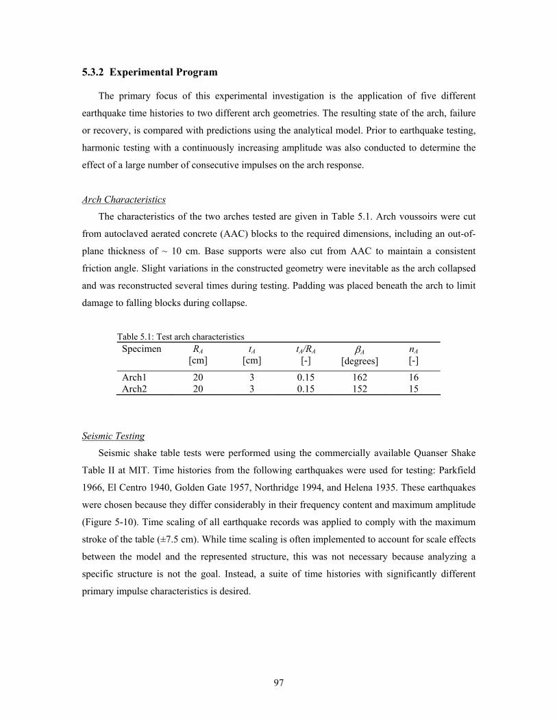
97

5.3.2 Experimental Program

The primary focus of this experimental investigation is the application of five different

earthquake time histories to two different arch geometries. The resulting state of the arch, failure

or recovery, is compared with predictions using the analytical model. Prior to earthquake testing,

harmonic testing with a continuously increasing amplitude was also conducted to determine the

effect of a large number of consecutive impulses on the arch response.

Arch Characteristics

The characteristics of the two arches tested are given in Table 5.1. Arch voussoirs were cut

from autoclaved aerated concrete (AAC) blocks to the required dimensions, including an out-of-

plane thickness of ~ 10 cm. Base supports were also cut from AAC to maintain a consistent

friction angle. Slight variations in the constructed geometry were inevitable as the arch collapsed

and was reconstructed several times during testing. Padding was placed beneath the arch to limit

damage to falling blocks during collapse.

Table 5.1: Test arch characteristics

Specimen RA [cm]

tA [cm]

tA/RA [-]

βA [degrees]

nA [-]

Arch1 20 3 0.15 162 16 Arch2 20 3 0.15 152 15

Seismic Testing

Seismic shake table tests were performed using the commercially available Quanser Shake

Table II at MIT. Time histories from the following earthquakes were used for testing: Parkfield

1966, El Centro 1940, Golden Gate 1957, Northridge 1994, and Helena 1935. These earthquakes

were chosen because they differ considerably in their frequency content and maximum amplitude

(Figure 5-10). Time scaling of all earthquake records was applied to comply with the maximum

stroke of the table (±7.5 cm). While time scaling is often implemented to account for scale effects

between the model and the represented structure, this was not necessary because analyzing a

specific structure is not the goal. Instead, a suite of time histories with significantly different

primary impulse characteristics is desired.

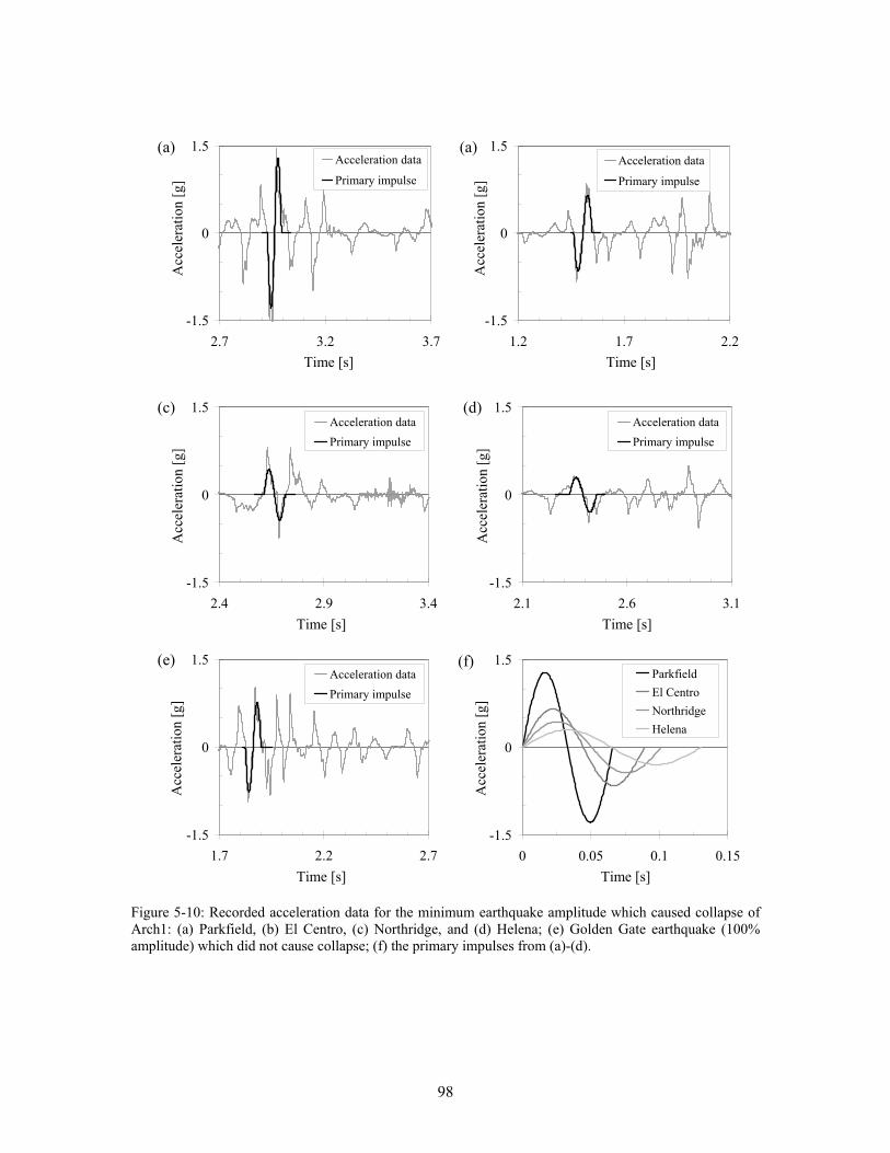
98

Figure 5-10: Recorded acceleration data for the minimum earthquake amplitude which caused collapse of Arch1: (a) Parkfield, (b) El Centro, (c) Northridge, and (d) Helena; (e) Golden Gate earthquake (100% amplitude) which did not cause collapse; (f) the primary impulses from (a)-(d).

-1.5

0

1.5

2.7 3.2 3.7Time [s]

Acc

eler

atio

n [g

]Acceleration data

Primary impulse

-1.5

0

1.5

1.2 1.7 2.2Time [s]

Acc

eler

atio

n [g

]

Acceleration data

Primary impulse

-1.5

0

1.5

2.1 2.6 3.1Time [s]

Acc

eler

atio

n [g

]

Acceleration dataPrimary impulse

-1.5

0

1.5

2.4 2.9 3.4Time [s]

Acc

eler

atio

n [g

]


-1.5

0

1.5

1.7 2.2 2.7Time [s]

Acc

eler

atio

n [g

]


(a)

(e)

Time [s]

Acc

eler

atio

n [g

]

Time [s]

Acc

eler

atio

n [g

]

(a)

Time [s]

Acc

eler

atio

n [g

]

(c)

Time [s]

Acc

eler

atio

n [g

]

(d)

Time [s]

Acc

eler

atio

n [g

]

-1.5

0

1.5

0 0.05 0.1 0.15Time [s]

Acc

eler

atio

n [g

]

ParkfieldEl CentroNorthridgeHelena

Time [s]

Acc

eler

atio

n [g

]

(f)

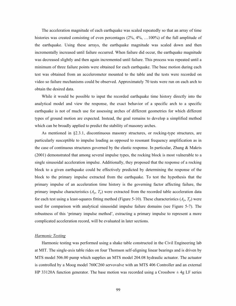
99

The acceleration magnitude of each earthquake was scaled repeatedly so that an array of time

histories was created consisting of even percentages (2%, 4%, …100%) of the full amplitude of

the earthquake. Using these arrays, the earthquake magnitude was scaled down and then

incrementally increased until failure occurred. When failure did occur, the earthquake magnitude

was decreased slightly and then again incremented until failure. This process was repeated until a

minimum of three failure points were obtained for each earthquake. The base motion during each

test was obtained from an accelerometer mounted to the table and the tests were recorded on

video so failure mechanisms could be observed. Approximately 70 tests were run on each arch to

obtain the desired data.

While it would be possible to input the recorded earthquake time history directly into the

analytical model and view the response, the exact behavior of a specific arch to a specific

earthquake is not of much use for assessing arches of different geometries for which different

types of ground motion are expected. Instead, the goal remains to develop a simplified method

which can be broadly applied to predict the stability of masonry arches.

As mentioned in §2.3.1, discontinuous masonry structures, or rocking-type structures, are

particularly susceptible to impulse loading as opposed to resonant frequency amplification as in

the case of continuous structures governed by the elastic response. In particular, Zhang & Makris

(2001) demonstrated that among several impulse types, the rocking block is most vulnerable to a

single sinusoidal acceleration impulse. Additionally, they proposed that the response of a rocking

block to a given earthquake could be effectively predicted by determining the response of the

block to the primary impulse extracted from the earthquake. To test the hypothesis that the

primary impulse of an acceleration time history is the governing factor affecting failure, the

primary impulse characteristics (Ap, Tp) were extracted from the recorded table acceleration data

for each test using a least-squares fitting method (Figure 5-10). These characteristics (Ap, Tp) were

used for comparison with analytical sinusoidal impulse failure domains (see Figure 5-7). The

robustness of this ‘primary impulse method’, extracting a primary impulse to represent a more

complicated acceleration record, will be evaluated in later sections.

Harmonic Testing

Harmonic testing was performed using a shake table constructed in the Civil Engineering lab

at MIT. The single-axis table rides on four Thomson self-aligning linear bearings and is driven by

MTS model 506.00 pump which supplies an MTS model 204.08 hydraulic actuator. The actuator

is controlled by a Moog model 760C260 servovalve with an MTS 406 Controller and an external

HP 33120A function generator. The base motion was recorded using a Crossbow ± 4g LF series

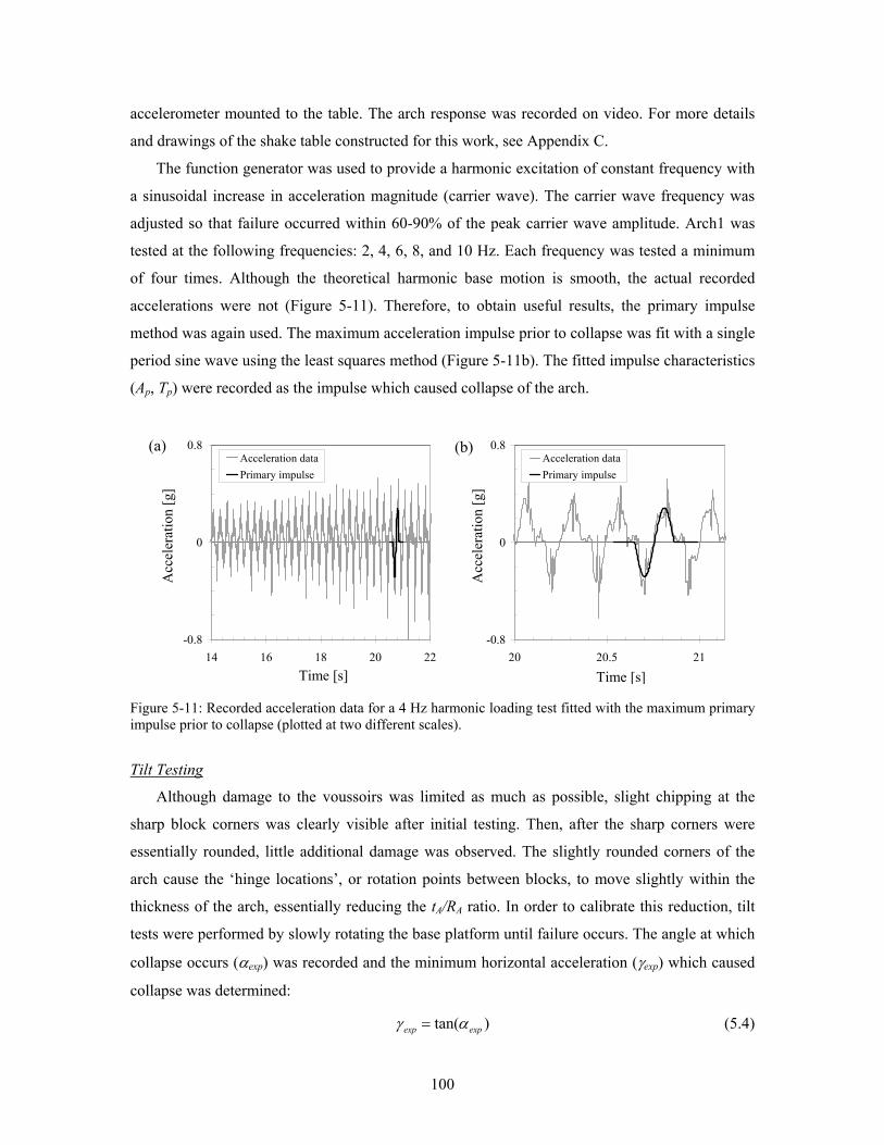
100

accelerometer mounted to the table. The arch response was recorded on video. For more details

and drawings of the shake table constructed for this work, see Appendix C.

The function generator was used to provide a harmonic excitation of constant frequency with

a sinusoidal increase in acceleration magnitude (carrier wave). The carrier wave frequency was

adjusted so that failure occurred within 60-90% of the peak carrier wave amplitude. Arch1 was

tested at the following frequencies: 2, 4, 6, 8, and 10 Hz. Each frequency was tested a minimum

of four times. Although the theoretical harmonic base motion is smooth, the actual recorded

accelerations were not (Figure 5-11). Therefore, to obtain useful results, the primary impulse

method was again used. The maximum acceleration impulse prior to collapse was fit with a single

period sine wave using the least squares method (Figure 5-11b). The fitted impulse characteristics

(Ap, Tp) were recorded as the impulse which caused collapse of the arch.

Figure 5-11: Recorded acceleration data for a 4 Hz harmonic loading test fitted with the maximum primary impulse prior to collapse (plotted at two different scales).

Tilt Testing

Although damage to the voussoirs was limited as much as possible, slight chipping at the

sharp block corners was clearly visible after initial testing. Then, after the sharp corners were

essentially rounded, little additional damage was observed. The slightly rounded corners of the

arch cause the ‘hinge locations’, or rotation points between blocks, to move slightly within the

thickness of the arch, essentially reducing the tA/RA ratio. In order to calibrate this reduction, tilt

tests were performed by slowly rotating the base platform until failure occurs. The angle at which

collapse occurs (αexp) was recorded and the minimum horizontal acceleration (γexp) which caused

collapse was determined:

tan( )=exp expγ α (5.4)

-0.8

0

0.8

20 20.5 21

Acc

eler

atio

n [g

]Acceleration dataPrimary impulse

-0.8

0

0.8

14 16 18 20 22

Acc

eler

atio

n [g

]


(a)

Time [s]

Acc

eler

atio

n [g

]

Acc

eler

atio

n [g

]

(b)

Time [s]

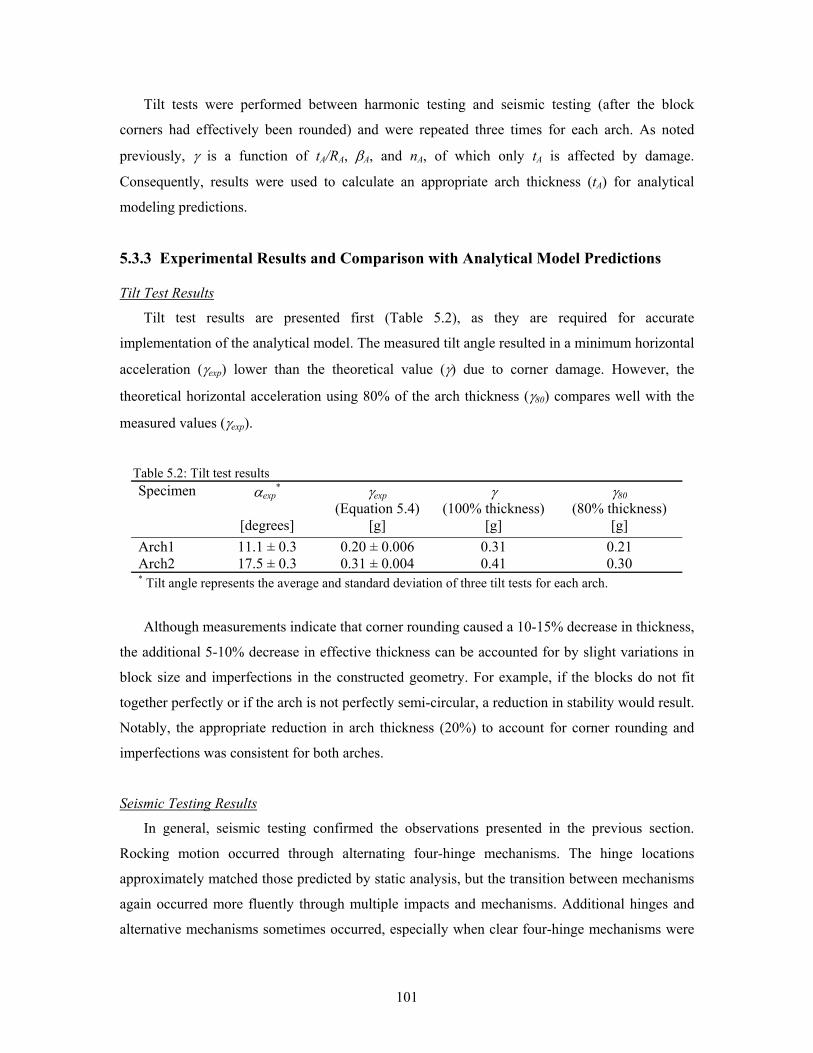
101

Tilt tests were performed between harmonic testing and seismic testing (after the block

corners had effectively been rounded) and were repeated three times for each arch. As noted

previously, γ is a function of tA/RA, βA, and nA, of which only tA is affected by damage.

Consequently, results were used to calculate an appropriate arch thickness (tA) for analytical

modeling predictions.

5.3.3 Experimental Results and Comparison with Analytical Model Predictions

Tilt Test Results

Tilt test results are presented first (Table 5.2), as they are required for accurate

implementation of the analytical model. The measured tilt angle resulted in a minimum horizontal

acceleration (γexp) lower than the theoretical value (γ) due to corner damage. However, the

theoretical horizontal acceleration using 80% of the arch thickness (γ80) compares well with the

measured values (γexp).

Table 5.2: Tilt test results

Specimen αexp*

[degrees]

γexp (Equation 5.4)

[g]

γ (100% thickness)

[g]

γ80 (80% thickness)

[g] Arch1 11.1 ± 0.3 0.20 ± 0.006 0.31 0.21 Arch2 17.5 ± 0.3 0.31 ± 0.004 0.41 0.30 * Tilt angle represents the average and standard deviation of three tilt tests for each arch.

Although measurements indicate that corner rounding caused a 10-15% decrease in thickness,

the additional 5-10% decrease in effective thickness can be accounted for by slight variations in

block size and imperfections in the constructed geometry. For example, if the blocks do not fit

together perfectly or if the arch is not perfectly semi-circular, a reduction in stability would result.

Notably, the appropriate reduction in arch thickness (20%) to account for corner rounding and

imperfections was consistent for both arches.

Seismic Testing Results

In general, seismic testing confirmed the observations presented in the previous section.

Rocking motion occurred through alternating four-hinge mechanisms. The hinge locations

approximately matched those predicted by static analysis, but the transition between mechanisms

again occurred more fluently through multiple impacts and mechanisms. Additional hinges and

alternative mechanisms sometimes occurred, especially when clear four-hinge mechanisms were

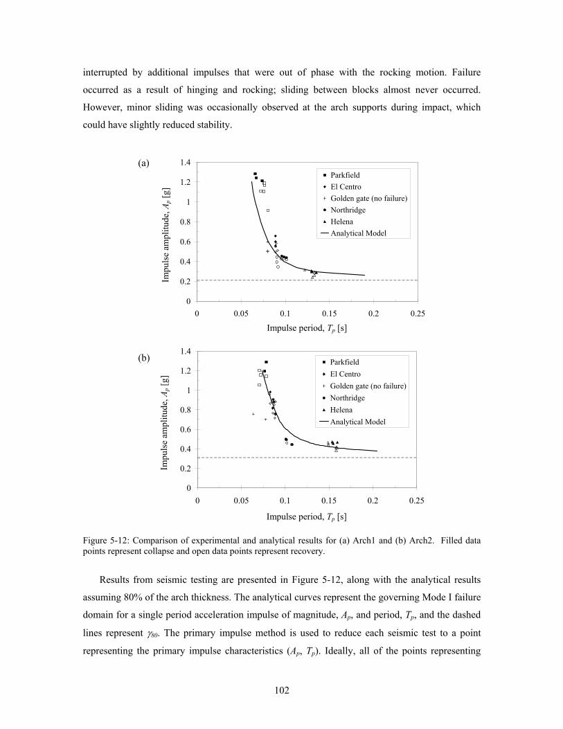
102

interrupted by additional impulses that were out of phase with the rocking motion. Failure

occurred as a result of hinging and rocking; sliding between blocks almost never occurred.

However, minor sliding was occasionally observed at the arch supports during impact, which

could have slightly reduced stability.

Figure 5-12: Comparison of experimental and analytical results for (a) Arch1 and (b) Arch2. Filled data points represent collapse and open data points represent recovery.

Results from seismic testing are presented in Figure 5-12, along with the analytical results

assuming 80% of the arch thickness. The analytical curves represent the governing Mode I failure

domain for a single period acceleration impulse of magnitude, Ap, and period, Tp, and the dashed

lines represent γ80. The primary impulse method is used to reduce each seismic test to a point

representing the primary impulse characteristics (Ap, Tp). Ideally, all of the points representing

0

0.2

0.4

0.6

0.8

1

1.2

1.4

0 0.05 0.1 0.15 0.2 0.25


Impu

lse

acce

lera

tion,

Ap

[g]

ParkfieldEl CentroGolden gate (no failure)NorthridgeHelenaAnalytical Model

0

0.2

0.4

0.6

0.8

1

1.2

1.4

0 0.05 0.1 0.15 0.2 0.25

Impulse period, T p [s]

Impu

lse

ampl

itude

, Ap

[g]

ParkfieldEl CentroGolden gate (no failure)NorthridgeHelenaAnalytical Model

(a)

(b)



Impu

lse

ampl

itude

, Ap [

g]

Impu

lse

ampl

itude

, Ap [

g]

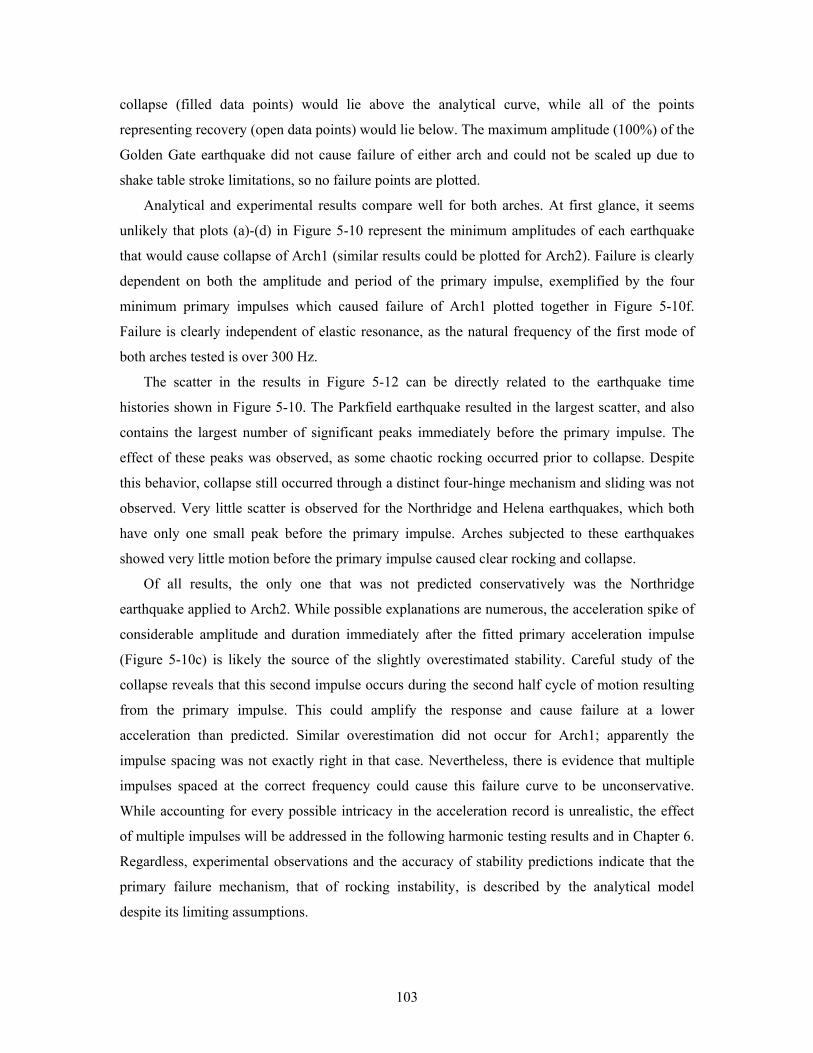
103

collapse (filled data points) would lie above the analytical curve, while all of the points

representing recovery (open data points) would lie below. The maximum amplitude (100%) of the

Golden Gate earthquake did not cause failure of either arch and could not be scaled up due to

shake table stroke limitations, so no failure points are plotted.

Analytical and experimental results compare well for both arches. At first glance, it seems

unlikely that plots (a)-(d) in Figure 5-10 represent the minimum amplitudes of each earthquake

that would cause collapse of Arch1 (similar results could be plotted for Arch2). Failure is clearly

dependent on both the amplitude and period of the primary impulse, exemplified by the four

minimum primary impulses which caused failure of Arch1 plotted together in Figure 5-10f.

Failure is clearly independent of elastic resonance, as the natural frequency of the first mode of

both arches tested is over 300 Hz.

The scatter in the results in Figure 5-12 can be directly related to the earthquake time

histories shown in Figure 5-10. The Parkfield earthquake resulted in the largest scatter, and also

contains the largest number of significant peaks immediately before the primary impulse. The

effect of these peaks was observed, as some chaotic rocking occurred prior to collapse. Despite

this behavior, collapse still occurred through a distinct four-hinge mechanism and sliding was not

observed. Very little scatter is observed for the Northridge and Helena earthquakes, which both

have only one small peak before the primary impulse. Arches subjected to these earthquakes

showed very little motion before the primary impulse caused clear rocking and collapse.

Of all results, the only one that was not predicted conservatively was the Northridge

earthquake applied to Arch2. While possible explanations are numerous, the acceleration spike of

considerable amplitude and duration immediately after the fitted primary acceleration impulse

(Figure 5-10c) is likely the source of the slightly overestimated stability. Careful study of the

collapse reveals that this second impulse occurs during the second half cycle of motion resulting

from the primary impulse. This could amplify the response and cause failure at a lower

acceleration than predicted. Similar overestimation did not occur for Arch1; apparently the

impulse spacing was not exactly right in that case. Nevertheless, there is evidence that multiple

impulses spaced at the correct frequency could cause this failure curve to be unconservative.

While accounting for every possible intricacy in the acceleration record is unrealistic, the effect

of multiple impulses will be addressed in the following harmonic testing results and in Chapter 6.

Regardless, experimental observations and the accuracy of stability predictions indicate that the

primary failure mechanism, that of rocking instability, is described by the analytical model

despite its limiting assumptions.

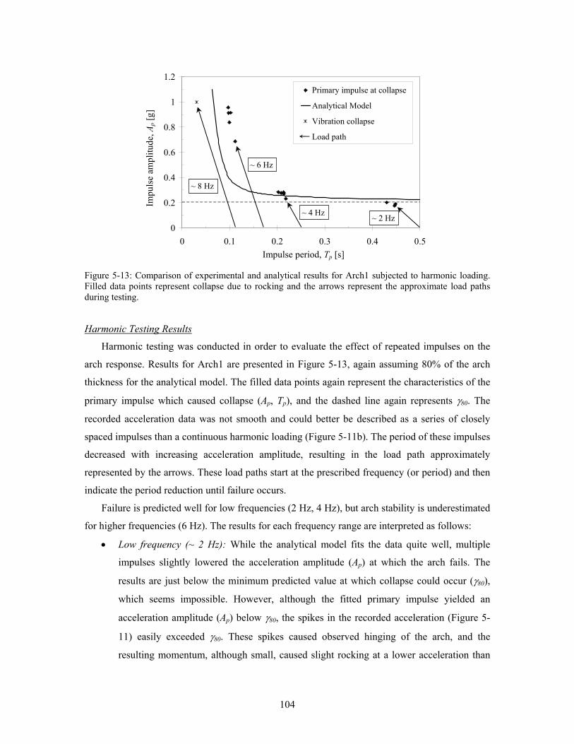
104

Figure 5-13: Comparison of experimental and analytical results for Arch1 subjected to harmonic loading. Filled data points represent collapse due to rocking and the arrows represent the approximate load paths during testing.

Harmonic Testing Results

Harmonic testing was conducted in order to evaluate the effect of repeated impulses on the

arch response. Results for Arch1 are presented in Figure 5-13, again assuming 80% of the arch

thickness for the analytical model. The filled data points again represent the characteristics of the

primary impulse which caused collapse (Ap, Tp), and the dashed line again represents γ80. The

recorded acceleration data was not smooth and could better be described as a series of closely

spaced impulses than a continuous harmonic loading (Figure 5-11b). The period of these impulses

decreased with increasing acceleration amplitude, resulting in the load path approximately

represented by the arrows. These load paths start at the prescribed frequency (or period) and then

indicate the period reduction until failure occurs.

Failure is predicted well for low frequencies (2 Hz, 4 Hz), but arch stability is underestimated

for higher frequencies (6 Hz). The results for each frequency range are interpreted as follows:

• Low frequency (~ 2 Hz): While the analytical model fits the data quite well, multiple

impulses slightly lowered the acceleration amplitude (Ap) at which the arch fails. The

results are just below the minimum predicted value at which collapse could occur (γ80),

which seems impossible. However, although the fitted primary impulse yielded an

acceleration amplitude (Ap) below γ80, the spikes in the recorded acceleration (Figure 5-

11) easily exceeded γ80. These spikes caused observed hinging of the arch, and the

resulting momentum, although small, caused slight rocking at a lower acceleration than

0

0.2

0.4

0.6

0.8

1

1.2

0 0.1 0.2 0.3 0.4 0.5Pulse Period, tp [s]

Puls

e A

ccel

erat

ion,

ap

/ g

Primary impulse at collapse

Analytical Model

Vibration collapse

Load path


Impu

lse

ampl

itude

, Ap [

g]

~ 8 Hz

~ 6 Hz

~ 4 Hz ~ 2 Hz

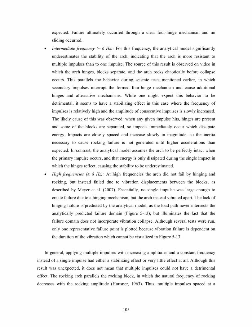
105

expected. Failure ultimately occurred through a clear four-hinge mechanism and no

sliding occurred.

• Intermediate frequency (~ 6 Hz): For this frequency, the analytical model significantly

underestimates the stability of the arch, indicating that the arch is more resistant to

multiple impulses than to one impulse. The source of this result is observed on video in

which the arch hinges, blocks separate, and the arch rocks chaotically before collapse

occurs. This parallels the behavior during seismic tests mentioned earlier, in which

secondary impulses interrupt the formed four-hinge mechanism and cause additional

hinges and alternative mechanisms. While one might expect this behavior to be

detrimental, it seems to have a stabilizing effect in this case where the frequency of

impulses is relatively high and the amplitude of consecutive impulses is slowly increased.

The likely cause of this was observed: when any given impulse hits, hinges are present

and some of the blocks are separated, so impacts immediately occur which dissipate

energy. Impacts are closely spaced and increase slowly in magnitude, so the inertia

necessary to cause rocking failure is not generated until higher accelerations than

expected. In contrast, the analytical model assumes the arch to be perfectly intact when

the primary impulse occurs, and that energy is only dissipated during the single impact in

which the hinges reflect, causing the stability to be underestimated.

• High frequencies (≥ 8 Hz): At high frequencies the arch did not fail by hinging and

rocking, but instead failed due to vibration displacements between the blocks, as

described by Meyer et al. (2007). Essentially, no single impulse was large enough to

create failure due to a hinging mechanism, but the arch instead vibrated apart. The lack of

hinging failure is predicted by the analytical model, as the load path never intersects the

analytically predicted failure domain (Figure 5-13), but illuminates the fact that the

failure domain does not incorporate vibration collapse. Although several tests were run,

only one representative failure point is plotted because vibration failure is dependent on

the duration of the vibration which cannot be visualized in Figure 5-13.

In general, applying multiple impulses with increasing amplitudes and a constant frequency

instead of a single impulse had either a stabilizing effect or very little effect at all. Although this

result was unexpected, it does not mean that multiple impulses could not have a detrimental

effect. The rocking arch parallels the rocking block, in which the natural frequency of rocking

decreases with the rocking amplitude (Housner, 1963). Thus, multiple impulses spaced at a

106

decreasing frequency would be more likely to act together to amplify the response, and lower the

impulse magnitude necessary to cause collapse. These concepts are explored further in Chapter 6.

5.4 Towards an Assessment Criterion for Arches

Although the analytical model has been shown to be effective in predicting collapse, it is of

little use if a prohibitive amount of work is required to obtain a first-order failure curve for each

possible arch geometry. Thus, working towards an applicable tool for assessment of existing

arches, the analytical model is used as a basis to develop a suite of failure curves which predict

the stability of a wide range of arch geometries.

5.4.1 Derivation of the Assessment Criterion

The analytical failure curves in Figures 5-12 and 5-13 were developed by repeatedly running

the analytical model for a range of impulse accelerations and periods. Because this is time-

intensive, fitting an equation to the failure curve is attractive for repeated use. While several

fitting methods were attempted, the following power curve which asymptotically approaches the

experimentally measured minimum acceleration necessary to cause collapse (γexp) was most

effective:

( ) 2

1= − +Cp

p min exp

AC T T

gγ (5.5)

where C1, C2, and Tmin are fitting coefficients. The fitted curves for the two arch geometries tested

are shown in Figure 5-14. For Arch1, C1 = 0.00252, C2 = -1.51, and Tmin = 0.044. For Arch2, C1 =

0.00674, C2 = -1.18, and Tmin = 0.060.

Once the fitted failure domain is obtained, it is convenient to use dimensional analysis to

extend the failure domain to any scale. Initially, the physical variables of the analytical model can

be used to write an equation of the form: ( , , , , , , ) 0=p p A A A AF A T g R t nβ , where F is a function of

the m previously defined variables. Note that the physical variables exist in only two fundamental

dimensions: length and time. Hence, two dimensionally independent variables (Tp , RA) are used

to create five (m - 2) dimensionless products (π-terms) which represent the complete set of

physical variables. For the analytical model to remain dimensionally homogeneous:

2 2

1 2 3 4 5, , , , 0⎛ ⎞

= = = = = =⎜ ⎟⎜ ⎟⎝ ⎠

p p p A

A A A

A T gT tG nR R R

π π π π β π (5.6)

107

Figure 5-14: Comparison of the analytical failure points for Arch1 and Arch2 to the fitted failure curves (Equation 5.5) and the assessment criterion failure curves (Equation 5.8).

For complete similarity between scales, the dimensionless products in Equation 5.6 must

remain constant at all scales. While π3, π4, and π5 are unaffected by scale, π1 and π2 are affected.

Using π2, the known similitude requirement that the time must be scaled by the square root of the

scale factor (Harris and Sabnis 1999) is derived:

,2 ,1 ,2 ,1=p p A AT T R R (5.7)

where the subscript 1 indicates the original scale and the subscript 2 indicates the new scale. Note

that Equation 5.7 also fulfills the similitude requirement for π1. This scaling relation was also

mentioned in §5.2.2, by Housner (1963) for the rocking block, and by Oppenheim (1992) for the

arch. While this scaling relation is expected, dimensional analysis clearly demonstrates that

material properties (density, elasticity, strength, etc.) do not enter the problem, so no other scaling

relationship is necessary.

Failure curves can now be calculated and fit at a single scale (RA = 1 m), and then easily

extended to any other scale. The following failure curve results:

1

2⎛ ⎞= − +⎜ ⎟⎜ ⎟

⎝ ⎠

p pmin

A

CA T

C Tg R

γ (5.8)

where RA is the centerline radius in meters, Tp is in seconds, and C1, C2, and Tmin are fitting

coefficients which need to be defined.

0

0.2

0.4

0.6

0.8

1

1.2

1.4

0 0.05 0.1 0.15 0.2 0.25Pulse Period, tp [s]

Puls

e A

ccel

erat

ion,

ap

/ g

Arch1 (analytical)

Arch2 (analytical)

Fit of analytical data

Assessment criterion


Impu

lse

ampl

itude

, Ap [

g]

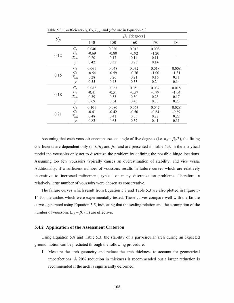
108

Table 5.3: Coefficients C1, C2, Tmin, and γ for use in Equation 5.8. βA [degrees] t

R

140 150 160 170 180

0.12

C1 C2

Tmin γ

0.040 -0.69 0.20 0.42

0.030 -0.80 0.17 0.32

0.018 -0.92 0.14 0.23

0.008 -1.20 0.11 0.14

-

0.15

C1 C2

Tmin γ

0.061 -0.54 0.28 0.55

0.048 -0.59 0.26 0.43

0.032 -0.76 0.21 0.33

0.018 -1.00 0.16 0.24

0.008 -1.31 0.11 0.14

0.18

C1 C2

Tmin γ

0.082 -0.41 0.39 0.69

0.063 -0.51 0.33 0.54

0.050 -0.57 0.30 0.43

0.032 -0.79 0.23 0.33

0.018 -1.04 0.17 0.23

0.21

C1 C2

Tmin γ

0.101 -0.41 0.48 0.82

0.080 -0.42 0.41 0.65

0.063 -0.50 0.35 0.52

0.047 -0.64 0.28 0.41

0.028 -0.89 0.22 0.31

Assuming that each voussoir encompasses an angle of five degrees (i.e. nA = βA/5), the fitting

coefficients are dependent only on tA/RA and βA, and are presented in Table 5.3. In the analytical

model the voussoirs only act to discretize the problem by defining the possible hinge locations.

Assuming too few voussoirs typically causes an overestimation of stability, and vice versa.

Additionally, if a sufficient number of voussoirs results in failure curves which are relatively

insensitive to increased refinement, typical of many discretization problems. Therefore, a

relatively large number of voussoirs were chosen as conservative.

The failure curves which result from Equation 5.8 and Table 5.3 are also plotted in Figure 5-

14 for the arches which were experimentally tested. These curves compare well with the failure

curves generated using Equation 5.5, indicating that the scaling relation and the assumption of the

number of voussoirs (nA = βA / 5) are effective.

5.4.2 Application of the Assessment Criterion

Using Equation 5.8 and Table 5.3, the stability of a part-circular arch during an expected

ground motion can be predicted through the following procedure:

1. Measure the arch geometry and reduce the arch thickness to account for geometrical

imperfections. A 20% reduction in thickness is recommended but a larger reduction is

recommended if the arch is significantly deformed.

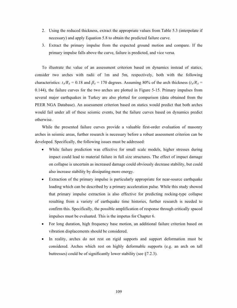
109

2. Using the reduced thickness, extract the appropriate values from Table 5.3 (interpolate if

necessary) and apply Equation 5.8 to obtain the predicted failure curve.

3. Extract the primary impulse from the expected ground motion and compare. If the

primary impulse falls above the curve, failure is predicted, and vice versa.

To illustrate the value of an assessment criterion based on dynamics instead of statics,

consider two arches with radii of 1m and 5m, respectively, both with the following

characteristics: tA/RA = 0.18 and βA = 170 degrees. Assuming 80% of the arch thickness (tA/RA =

0.144), the failure curves for the two arches are plotted in Figure 5-15. Primary impulses from

several major earthquakes in Turkey are also plotted for comparison (data obtained from the

PEER NGA Database). An assessment criterion based on statics would predict that both arches

would fail under all of these seismic events, but the failure curves based on dynamics predict

otherwise.

While the presented failure curves provide a valuable first-order evaluation of masonry

arches in seismic areas, further research is necessary before a robust assessment criterion can be

developed. Specifically, the following issues must be addressed:

• While failure prediction was effective for small scale models, higher stresses during

impact could lead to material failure in full size structures. The effect of impact damage

on collapse is uncertain as increased damage could obviously decrease stability, but could

also increase stability by dissipating more energy.

• Extraction of the primary impulse is particularly appropriate for near-source earthquake

loading which can be described by a primary acceleration pulse. While this study showed

that primary impulse extraction is also effective for predicting rocking-type collapse

resulting from a variety of earthquake time histories, further research is needed to

confirm this. Specifically, the possible amplification of response through critically spaced

impulses must be evaluated. This is the impetus for Chapter 6.

• For long duration, high frequency base motion, an additional failure criterion based on

vibration displacements should be considered.

• In reality, arches do not rest on rigid supports and support deformation must be

considered. Arches which rest on highly deformable supports (e.g. an arch on tall

buttresses) could be of significantly lower stability (see §7.2.3).

110

Figure 5-15: Predicted failure domains for two arches with radii (RA) of 1m and 5m, both with tA / RA = 0.18 and βA = 170 degrees, compared with primary impulses extracted from acceleration data from major earthquakes in Turkey (PEER NGA Database record number in parentheses).

5.5 Summary

The proposed analytical model presented in §5.2 and the experimental investigation discussed

in §5.3 provide new insight into the dynamic behavior of masonry arches under base motion. Of

primary importance, the rocking behavior of arches is described and modeled for the first time.

Through this investigation, the following conclusions are drawn:

• For an arch subjected to a single horizontal base impulse, Mode I collapse governs, i.e.

collapse during the second half cycle of motion, after a single impact has occurred.

Therefore, the Mode `I failure curve should be used for design and assessment purposes.

• Larger scale arches are more resistant to ground motions than smaller arches with the

same geometrical proportions. Additionally, for an arch of a given scale, the stability of

the arch increases as tA/RA increases or βA decreases.

• The minimum coefficient of friction theoretically required to prevent sliding is below the

typical values of masonry joints, and hence the assumption of no sliding is reasonable.

• The primary impulse method, extracting the primary impulse of an acceleration record,

provided accurate failure predictions for the arches tested. In the process, further

evidence that rocking type structures are particularly vulnerable to impulse-type base

motions was presented. Additionally, the acceleration magnitude and period of the

0

0.2

0.4

0.6

0.8

1

0 0.2 0.4 0.6 0.8 1Pulse Period, tp [s]

Puls

e A

ccel

erat

ion,

ap

/ g

Failure curve ( = 5m)Failure curve ( = 1m)Dinar, 1995 (NGA1141)Duzce, 1999 (NGA1602)Erzican, 1992 (NGA0821)Izmir, 1977 (NGA0134)Kocaeli, 1999 (NGA1158)

RA

RA


Impu

lse

ampl

itude

, Ap [

g]

111

impulse were both shown to be critical in causing failure. Possible effects of multiple

impulses were observed, and will be investigated further in Chapter 6.

The effectiveness of the analytical model in predicting experimental results led to the

development of a suite of failure curves which predict the rocking stability of a range of masonry

arch geometries (§5.4). While the failure curves accurately predicted failure of the small scale

arches tested, application to full scale structures requires further research. Several areas of future

research have been specifically identified, and could lead to a rapid assessment tool which would

be of great utility for evaluating the safety of vaulted masonry structures around the world.

In conclusion, the characterization of rocking arch failure presented in this chapter

exemplifies the merits of analytical dynamics as a tool for assessing masonry structures. If the

essence of dynamic behavior can be captured by analytical models of reasonable complexity, then

the method is appropriate and powerful.

112

Chapter 6

Analytical Modeling: Rocking Structures

6.1 Introduction

The rocking response to horizontal ground motion remains a concern in the seismic

assessment of a variety of masonry structures: monuments, towers, statues, bridge piers,

sculptures, etc. Chapter 5 adds the arch to this category, and inspires further investigation into the

nature of rocking structures. Specifically, the evidence that the primary impulse is critically

important for these structures beckons further inquiry into the ground motions to which rocking

structures are most vulnerable. Despite a significant amount of research in this area, engineers

still sometimes misunderstand the fundamental difference between the dynamic response of

rocking structures and typical elastic structures, and therefore assess rocking from a flawed

perspective. As a result, the fundamental behavior of rocking structures needs further

clarification.

As mentioned in §2.3.1, the seminal work on the rigid rocking block by Housner (1963) first

addressed the behavior of rocking structures, introducing a problem which has since attracted

widespread interest. Housner (1963) showed that the natural rocking period increases with

rocking angle, and evaluated the vulnerability of rocking structures to single square and sine

pulses. He also demonstrated overturning through multiple successive pulses by generating

earthquake motions as discrete step changes ±v in ground velocity and evaluating the probability

113

of collapse. He concluded that “…relatively small ground motion may fortuitously build up the

amplitude… and lead to overturning the block.”

This chapter addresses the response of rocking structures to horizontal ground motion from a

similar rigid body dynamics perspective. Building on the work of Makris and Konstantinidis

(2003), the goal is to further highlight the fundamental differences between rocking structures and

typical elastic structures, and to explore ground motions which would cause the maximum

amplification of rocking motion, or rocking resonance. To achieve this, an energy approach is

taken, where the primary concern is the rate of energy input in the system.

In §6.2, the mathematical formulation for the rocking block is first presented, and the rate of

energy input into the system is evaluated. Subsequently, the response of rocking structures which

are not at rest but have some initial motion or energy is investigated. The motivation for this is

twofold: 1) to explore the idea that at-rest stability is unconservative and unreliable if small initial

motions are generated during earthquakes, an idea which has not been considered in the literature,

and 2) to explore the ability of multiple impulses to amplify the rocking response, a behavior

which has not been directly addressed since it was suggested by Housner (1963). In §6.3, a

method of generating earthquake time histories using past earthquake data is presented and

applied to statistically determine the probability of collapse of the rocking block and the rocking

arch. In §6.4, conclusions are drawn.

6.2 An Energy Approach

Investigation of the fundamental behavior of rocking structures begins with the rocking

block. Following the work of Housner (1963), it is assumed that a rigid block rocks back and

forth about alternating bottom corner hinges (points O and O’ in Figure 6-1). The resulting

motion can be described by two dimensionless non-linear equations:

( ) ( ) ( )( ) ( ) ( )

sin / cos 0

sin / cos 0

′′ + − = − − >

′′ + − − = − − − <

cr g cr

cr g cr

u g for

u g for

θ θ θ θ θ θ

θ θ θ θ θ θ (6.1)

where θcr and θ are defined in Figure 6-1, gu is the ground acceleration, g is the acceleration of

gravity, and 2 / 2′′ = d dθ θ τ where 3 / (4 )= Bt g Rτ is the dimensionless time. The transition

between the equations of motion in Equation 6.1 occurs when the block passes through the rest

position (θ = 0) and the rotation point jumps to the opposing bottom corner. This transition is

accompanied by a decrease in energy due to impact, often described by a coefficient of

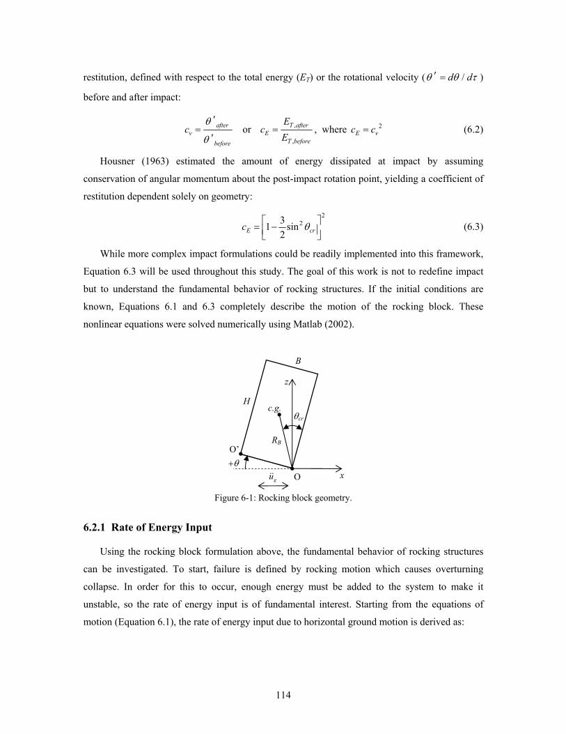
114

restitution, defined with respect to the total energy (ET) or the rotational velocity ( /′ = d dθ θ τ )

before and after impact:

′

=′

afterv

before

cθ

θ or ,

,= T after

ET before

Ec

E, where 2=E vc c (6.2)

Housner (1963) estimated the amount of energy dissipated at impact by assuming

conservation of angular momentum about the post-impact rotation point, yielding a coefficient of

restitution dependent solely on geometry:

2

231 sin2

⎡ ⎤= −⎢ ⎥⎣ ⎦E crc θ (6.3)

While more complex impact formulations could be readily implemented into this framework,

Equation 6.3 will be used throughout this study. The goal of this work is not to redefine impact

but to understand the fundamental behavior of rocking structures. If the initial conditions are

known, Equations 6.1 and 6.3 completely describe the motion of the rocking block. These

nonlinear equations were solved numerically using Matlab (2002).

Figure 6-1: Rocking block geometry.

6.2.1 Rate of Energy Input

Using the rocking block formulation above, the fundamental behavior of rocking structures

can be investigated. To start, failure is defined by rocking motion which causes overturning

collapse. In order for this to occur, enough energy must be added to the system to make it

unstable, so the rate of energy input is of fundamental interest. Starting from the equations of

motion (Equation 6.1), the rate of energy input due to horizontal ground motion is derived as:

x gu

H

z

RB

θcr

B

+θ

c.g.

O’

O

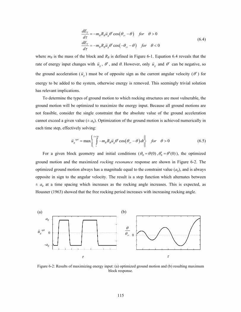
115

( )

( )

cos 0

cos 0

′= − − >

′= − − − <

TB B g cr

TB B g cr

dE m R u ford

dE m R u ford

θ θ θ θτ

θ θ θ θτ

(6.4)

where mB is the mass of the block and RB is defined in Figure 6-1. Equation 6.4 reveals that the

rate of energy input changes with gu , ′θ , and θ. However, only gu and ′θ can be negative, so

the ground acceleration ( gu ) must be of opposite sign as the current angular velocity ( ′θ ) for

energy to be added to the system, otherwise energy is removed. This seemingly trivial solution

has relevant implications.

To determine the types of ground motion to which rocking structures are most vulnerable, the

ground motion will be optimized to maximize the energy input. Because all ground motions are

not feasible, consider the single constraint that the absolute value of the ground acceleration

cannot exceed a given value (± ag). Optimization of the ground motion is achieved numerically in

each time step, effectively solving:

( )max cos 0+Δ⎧ ⎫⎪ ⎪′= − − >⎨ ⎬

⎪ ⎪⎩ ⎭∫

t topt

g B B g crt

u m R u dt forθ θ θ θ (6.5)

For a given block geometry and initial conditions ( 0 (0)=θ θ , 0 (0)′ ′=θ θ ), the optimized

ground motion and the maximized rocking resonance response are shown in Figure 6-2. The

optimized ground motion always has a magnitude equal to the constraint value (ag), and is always

opposite in sign to the angular velocity. The result is a step function which alternates between

± ag at a time spacing which increases as the rocking angle increases. This is expected, as

Housner (1963) showed that the free rocking period increases with increasing rocking angle.

Figure 6-2: Results of maximizing energy input: (a) optimized ground motion and (b) resulting maximum

block response.

(a) (b)

cr

θθ

τ

ag

-ag

optgu

τ

0 0

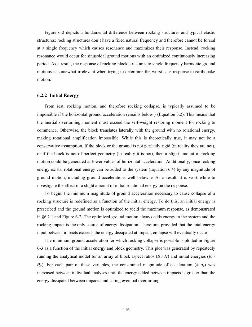
116

Figure 6-2 depicts a fundamental difference between rocking structures and typical elastic

structures: rocking structures don’t have a fixed natural frequency and therefore cannot be forced

at a single frequency which causes resonance and maximizes their response. Instead, rocking

resonance would occur for sinusoidal ground motions with an optimized continuously increasing

period. As a result, the response of rocking block structures to single frequency harmonic ground

motions is somewhat irrelevant when trying to determine the worst case response to earthquake

motion.

6.2.2 Initial Energy

From rest, rocking motion, and therefore rocking collapse, is typically assumed to be

impossible if the horizontal ground acceleration remains below γ (Equation 3.2). This means that

the inertial overturning moment must exceed the self-weight restoring moment for rocking to

commence. Otherwise, the block translates laterally with the ground with no rotational energy,

making rotational amplification impossible. While this is theoretically true, it may not be a

conservative assumption. If the block or the ground is not perfectly rigid (in reality they are not),

or if the block is not of perfect geometry (in reality it is not), then a slight amount of rocking

motion could be generated at lower values of horizontal acceleration. Additionally, once rocking

energy exists, rotational energy can be added to the system (Equation 6.4) by any magnitude of

ground motion, including ground accelerations well below γ. As a result, it is worthwhile to

investigate the effect of a slight amount of initial rotational energy on the response.

To begin, the minimum magnitude of ground acceleration necessary to cause collapse of a

rocking structure is redefined as a function of the initial energy. To do this, an initial energy is

prescribed and the ground motion is optimized to yield the maximum response, as demonstrated

in §6.2.1 and Figure 6-2. The optimized ground motion always adds energy to the system and the

rocking impact is the only source of energy dissipation. Therefore, provided that the total energy

input between impacts exceeds the energy dissipated at impact, collapse will eventually occur.

The minimum ground acceleration for which rocking collapse is possible is plotted in Figure

6-3 as a function of the initial energy and block geometry. This plot was generated by repeatedly

running the analytical model for an array of block aspect ratios (B / H) and initial energies (θo /

θcr). For each pair of these variables, the constrained magnitude of acceleration (± ag) was

increased between individual analyses until the energy added between impacts is greater than the

energy dissipated between impacts, indicating eventual overturning.

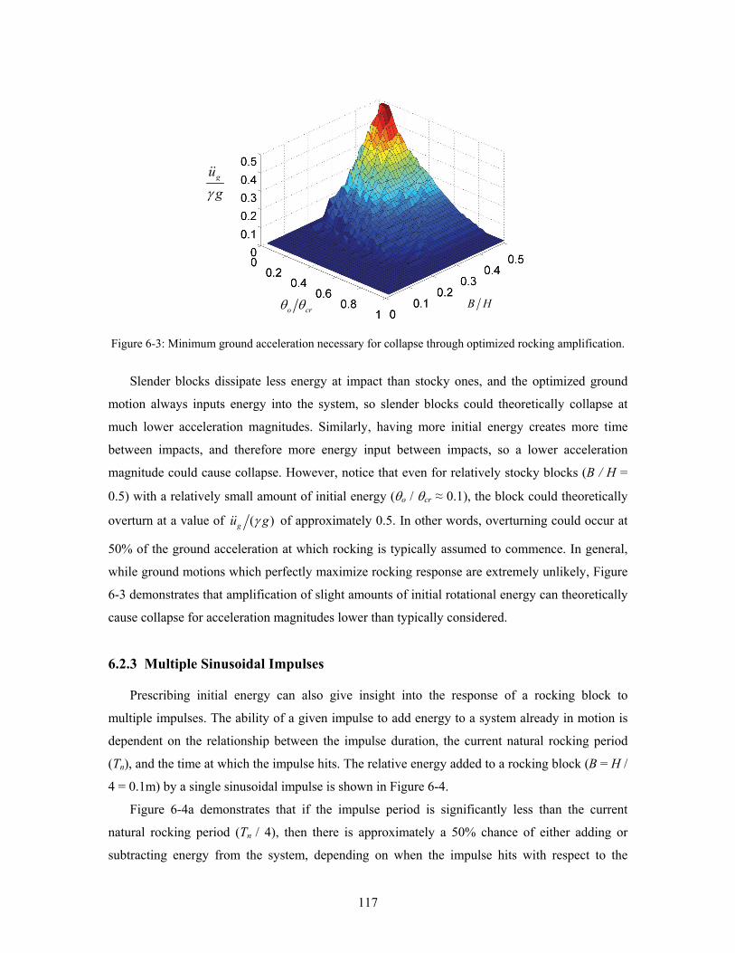
117

Figure 6-3: Minimum ground acceleration necessary for collapse through optimized rocking amplification.

Slender blocks dissipate less energy at impact than stocky ones, and the optimized ground

motion always inputs energy into the system, so slender blocks could theoretically collapse at

much lower acceleration magnitudes. Similarly, having more initial energy creates more time

between impacts, and therefore more energy input between impacts, so a lower acceleration

magnitude could cause collapse. However, notice that even for relatively stocky blocks (B / H =

0.5) with a relatively small amount of initial energy (θo / θcr ≈ 0.1), the block could theoretically

overturn at a value of ( )gu gγ of approximately 0.5. In other words, overturning could occur at

50% of the ground acceleration at which rocking is typically assumed to commence. In general,

while ground motions which perfectly maximize rocking response are extremely unlikely, Figure

6-3 demonstrates that amplification of slight amounts of initial rotational energy can theoretically

cause collapse for acceleration magnitudes lower than typically considered.

6.2.3 Multiple Sinusoidal Impulses

Prescribing initial energy can also give insight into the response of a rocking block to

multiple impulses. The ability of a given impulse to add energy to a system already in motion is

dependent on the relationship between the impulse duration, the current natural rocking period

(Tn), and the time at which the impulse hits. The relative energy added to a rocking block (B = H /

4 = 0.1m) by a single sinusoidal impulse is shown in Figure 6-4.

Figure 6-4a demonstrates that if the impulse period is significantly less than the current

natural rocking period (Tn / 4), then there is approximately a 50% chance of either adding or

subtracting energy from the system, depending on when the impulse hits with respect to the

gugγ

o crθ θ B H

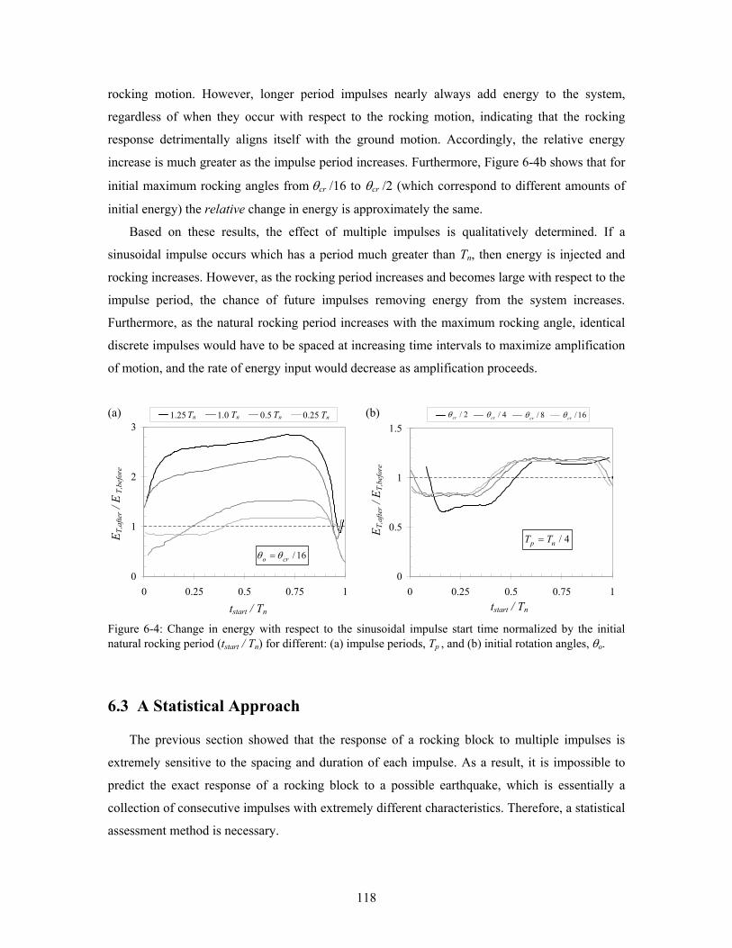
118

rocking motion. However, longer period impulses nearly always add energy to the system,

regardless of when they occur with respect to the rocking motion, indicating that the rocking

response detrimentally aligns itself with the ground motion. Accordingly, the relative energy

increase is much greater as the impulse period increases. Furthermore, Figure 6-4b shows that for

initial maximum rocking angles from θcr /16 to θcr /2 (which correspond to different amounts of

initial energy) the relative change in energy is approximately the same.

Based on these results, the effect of multiple impulses is qualitatively determined. If a

sinusoidal impulse occurs which has a period much greater than Tn, then energy is injected and

rocking increases. However, as the rocking period increases and becomes large with respect to the

impulse period, the chance of future impulses removing energy from the system increases.

Furthermore, as the natural rocking period increases with the maximum rocking angle, identical

discrete impulses would have to be spaced at increasing time intervals to maximize amplification

of motion, and the rate of energy input would decrease as amplification proceeds.

Figure 6-4: Change in energy with respect to the sinusoidal impulse start time normalized by the initial natural rocking period (tstart / Tn) for different: (a) impulse periods, Tp , and (b) initial rotation angles, θo.

6.3 A Statistical Approach

The previous section showed that the response of a rocking block to multiple impulses is

extremely sensitive to the spacing and duration of each impulse. As a result, it is impossible to

predict the exact response of a rocking block to a possible earthquake, which is essentially a

collection of consecutive impulses with extremely different characteristics. Therefore, a statistical

assessment method is necessary.

0

0.5

1

1.5

0 0.25 0.5 0.75 1tstart / Tn

Eafte

r / E

befo

re

0

1

2

3

0 0.25 0.5 0.75 1tstart / Tn

Eafte

r / E

befo

re

1.25 1.0 0.5 0.25

/ 16o crθ θ=

/ 4p nT T=

/ 2crθ / 4crθ / 8crθ / 16crθ(b) Tn Tn Tn Tn

tstart / Tn tstart / Tn

E T,a

fter /

E T

,bef

ore

E T,a

fter /

ET,

befo

re

(a)

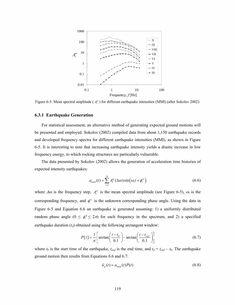
119

Figure 6-5: Mean spectral amplitude ( iAω ) for different earthquake intensities (MMI) (after Sokolov 2002).

6.3.1 Earthquake Generation

For statistical assessment, an alternative method of generating expected ground motions will

be presented and employed. Sokolov (2002) compiled data from about 1,150 earthquake records

and developed frequency spectra for different earthquake intensities (MMI), as shown in Figure

6-5. It is interesting to note that increasing earthquake intensity yields a drastic increase in low

frequency energy, to which rocking structures are particularly vulnerable.

The data presented by Sokolov (2002) allows the generation of acceleration time histories of

expected intensity earthquakes:

( )15

1

( ) ( )sin=

= Δ +∑total i i ii

a t A tω ωω ω φ (6.6)

where Δω is the frequency step, iAω is the mean spectral amplitude (see Figure 6-5), ωi is the

corresponding frequency, and iωφ is the unknown corresponding phase angle. Using the data in

Figure 6-5 and Equation 6.6 an earthquake is generated assuming: 1) a uniformly distributed

random phase angle (0 ≤ iωφ ≤ 2π) for each frequency in the spectrum, and 2) a specified

earthquake duration (td) obtained using the following arctangent window:

( ) 01 arctan arctan0.1 0.1

⎡ ⎤− −⎛ ⎞ ⎛ ⎞= −⎜ ⎟ ⎜ ⎟⎢ ⎥⎝ ⎠ ⎝ ⎠⎣ ⎦

endt t t tP tπ

(6.7)

where t0 is the start time of the earthquake, tend is the end time, and td = tend – t0. The earthquake

ground motion then results from Equations 6.6 and 6.7:

( ) ( ) ( )=g totalu t a t P t (6.8)

0.01

0.1

1

10

100

1000

0.1 1 10 100Frequency [Hz]

XIXVIIIVIIVIVIVIII

iAω

Frequency, f [Hz]

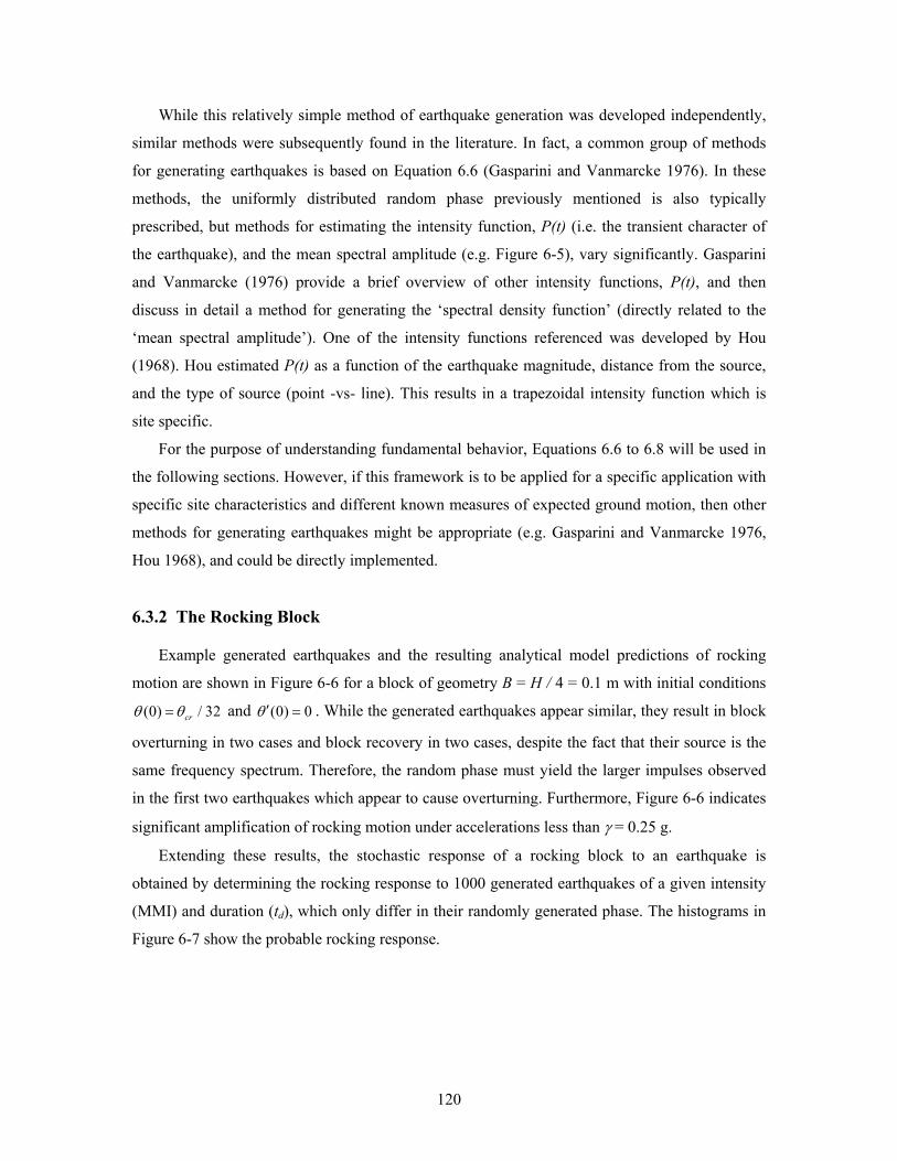
120

While this relatively simple method of earthquake generation was developed independently,

similar methods were subsequently found in the literature. In fact, a common group of methods

for generating earthquakes is based on Equation 6.6 (Gasparini and Vanmarcke 1976). In these

methods, the uniformly distributed random phase previously mentioned is also typically

prescribed, but methods for estimating the intensity function, P(t) (i.e. the transient character of

the earthquake), and the mean spectral amplitude (e.g. Figure 6-5), vary significantly. Gasparini

and Vanmarcke (1976) provide a brief overview of other intensity functions, P(t), and then

discuss in detail a method for generating the ‘spectral density function’ (directly related to the

‘mean spectral amplitude’). One of the intensity functions referenced was developed by Hou

(1968). Hou estimated P(t) as a function of the earthquake magnitude, distance from the source,

and the type of source (point -vs- line). This results in a trapezoidal intensity function which is

site specific.

For the purpose of understanding fundamental behavior, Equations 6.6 to 6.8 will be used in

the following sections. However, if this framework is to be applied for a specific application with

specific site characteristics and different known measures of expected ground motion, then other

methods for generating earthquakes might be appropriate (e.g. Gasparini and Vanmarcke 1976,

Hou 1968), and could be directly implemented.

6.3.2 The Rocking Block

Example generated earthquakes and the resulting analytical model predictions of rocking

motion are shown in Figure 6-6 for a block of geometry B = H / 4 = 0.1 m with initial conditions

(0) / 32= crθ θ and (0) 0′ =θ . While the generated earthquakes appear similar, they result in block

overturning in two cases and block recovery in two cases, despite the fact that their source is the

same frequency spectrum. Therefore, the random phase must yield the larger impulses observed

in the first two earthquakes which appear to cause overturning. Furthermore, Figure 6-6 indicates

significant amplification of rocking motion under accelerations less than γ = 0.25 g.

Extending these results, the stochastic response of a rocking block to an earthquake is

obtained by determining the rocking response to 1000 generated earthquakes of a given intensity

(MMI) and duration (td), which only differ in their randomly generated phase. The histograms in

Figure 6-7 show the probable rocking response.

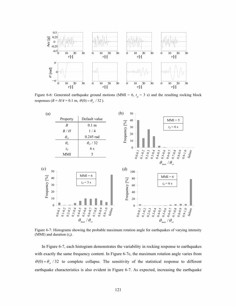
121

Figure 6-6: Generated earthquake ground motions (MMI = 6, td = 3 s) and the resulting rocking block responses (B = H/4 = 0.1 m, (0) / 32= crθ θ ).

Property Default value B 0.1 m

B / H 1 / 4 θcr 0.245 rad θo θcr / 32 td 6 s

MMI 5

Figure 6-7: Histograms showing the probable maximum rotation angle for earthquakes of varying intensity (MMI) and duration (td).

In Figure 6-7, each histogram demonstrates the variability in rocking response to earthquakes

with exactly the same frequency content. In Figure 6-7c, the maximum rotation angle varies from

(0) / 32= crθ θ to complete collapse. The sensitivity of the statistical response to different

earthquake characteristics is also evident in Figure 6-7. As expected, increasing the earthquake

0

20

40

60

80

100

0.0-

0.1

0.1-

0.2

0.2-

0.3

0.3-

0.4

0.4-

0.5

0.5-

0.6

0.6-

0.7

0.7-

0.8

0.8-

0.9

0.9-

1.0

failu

re

0

10

20

30

40

50

0.0-

0.1

0.1-

0.2

0.2-

0.3

0.3-

0.4

0.4-

0.5

0.5-

0.6

0.6-

0.7

0.7-

0.8

0.8-

0.9

0.9-

1.0

failu

re

MMI = 6

td = 3 s

/max crθ θ

(c)

MMI = 6

td = 6 s

/max crθ θ

(d)

Freq

uenc

y [%

]

Freq

uenc

y [%

]

0 10 20 30-0.5

-0.250

0.250.5

τ [-]

Acc

[g]

0 10 20 30

0

τ [-]

θ [r

ad]

0 10 20 30τ [-]

0 10 20 30τ [-]

0 10 20 30τ [-]

0 10 20 30τ [-]

0 10 20 30τ [-]

0 10 20 30τ [-]

α

α−

(a) (b)

0

10

20

30

40

50

0.0-

0.1

0.1-

0.2

0.2-

0.3

0.3-

0.4

0.4-

0.5

0.5-

0.6

0.6-

0.7

0.7-

0.8

0.8-

0.9

0.9-

1.0

failu

re

MMI = 5

td = 6 s

/max crθ θ

Freq

uenc

y [%

]

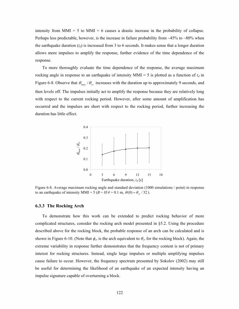
122

intensity from MMI = 5 to MMI = 6 causes a drastic increase in the probability of collapse.

Perhaps less predictable, however, is the increase in failure probability from ~45% to ~80% when

the earthquake duration (td) is increased from 3 to 6 seconds. It makes sense that a longer duration

allows more impulses to amplify the response, further evidence of the time dependence of the

response.

To more thoroughly evaluate the time dependence of the response, the average maximum

rocking angle in response to an earthquake of intensity MMI = 5 is plotted as a function of td in

Figure 6-8. Observe that /max crθ θ increases with the duration up to approximately 9 seconds, and

then levels off. The impulses initially act to amplify the response because they are relatively long

with respect to the current rocking period. However, after some amount of amplification has

occurred and the impulses are short with respect to the rocking period, further increasing the

duration has little effect.

Figure 6-8. Average maximum rocking angle and standard deviation (1000 simulations / point) in response to an earthquake of intensity MMI = 5 (B = H/4 = 0.1 m, (0) / 32= crθ θ ).

6.3.3 The Rocking Arch

To demonstrate how this work can be extended to predict rocking behavior of more

complicated structures, consider the rocking arch model presented in §5.2. Using the procedure

described above for the rocking block, the probable response of an arch can be calculated and is

shown in Figure 6-10. (Note that φcr is the arch equivalent to θcr for the rocking block). Again, the

extreme variability in response further demonstrates that the frequency content is not of primary

interest for rocking structures. Instead, single large impulses or multiple amplifying impulses

cause failure to occur. However, the frequency spectrum presented by Sokolov (2002) may still

be useful for determining the likelihood of an earthquake of an expected intensity having an

impulse signature capable of overturning a block.

0.0

0.1

0.2

0.3

0.4

0 3 6 9 12 15 18Impulse duration [s]

a

Earthquake duration, td [s]

θ max

/ θ c

r

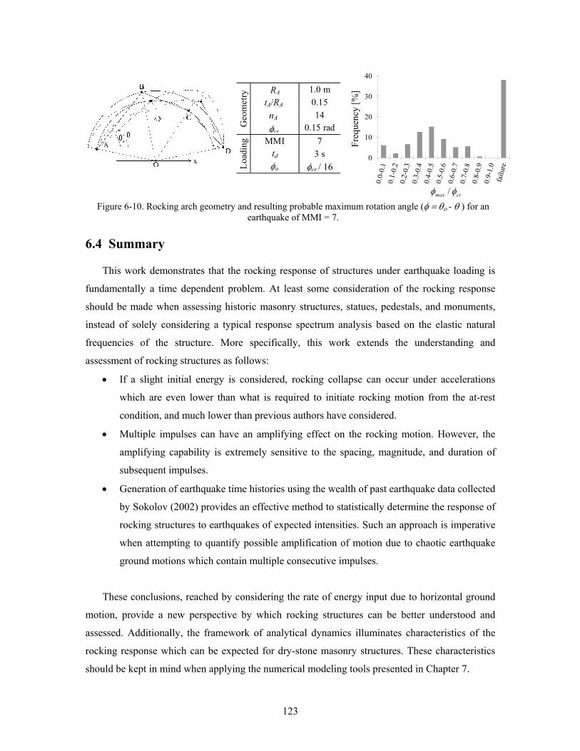
123

Figure 6-10. Rocking arch geometry and resulting probable maximum rotation angle (φ = θο - θ ) for an

earthquake of MMI = 7. 6.4 Summary

This work demonstrates that the rocking response of structures under earthquake loading is

fundamentally a time dependent problem. At least some consideration of the rocking response

should be made when assessing historic masonry structures, statues, pedestals, and monuments,

instead of solely considering a typical response spectrum analysis based on the elastic natural

frequencies of the structure. More specifically, this work extends the understanding and

assessment of rocking structures as follows:

• If a slight initial energy is considered, rocking collapse can occur under accelerations

which are even lower than what is required to initiate rocking motion from the at-rest

condition, and much lower than previous authors have considered.

• Multiple impulses can have an amplifying effect on the rocking motion. However, the

amplifying capability is extremely sensitive to the spacing, magnitude, and duration of

subsequent impulses.

• Generation of earthquake time histories using the wealth of past earthquake data collected

by Sokolov (2002) provides an effective method to statistically determine the response of

rocking structures to earthquakes of expected intensities. Such an approach is imperative

when attempting to quantify possible amplification of motion due to chaotic earthquake

ground motions which contain multiple consecutive impulses.

These conclusions, reached by considering the rate of energy input due to horizontal ground

motion, provide a new perspective by which rocking structures can be better understood and

assessed. Additionally, the framework of analytical dynamics illuminates characteristics of the

rocking response which can be expected for dry-stone masonry structures. These characteristics

should be kept in mind when applying the numerical modeling tools presented in Chapter 7.

0

10

20

30

40

0.0-

0.1

0.1-

0.2

0.2-

0.3

0.3-

0.4

0.4-

0.5

0.5-

0.6

0.6-

0.7

0.7-

0.8

0.8-

0.9

0.9-

1.0

failu

re

/max crφ φ

Freq

uenc

y [%

] Radius, R 1.0 m t / R 0.15

nblocks 14

Geo

met

ry

φcrit 0.15 rad MMI 7

duration 3 s

Load

ing

φo φcrit / 16

nA

tA/RA

RA

td

φcr

φcr / 16

124

Chapter 7

Discrete Element Modeling

7.1 Introduction

The previous two chapters have investigated the use of analytical models in assessing

masonry structures under horizontal ground motion. While these analytical models are effective

in predicting response, and provide valuable insight into the nature of the dynamics of rocking

structures, they are rather involved for relatively simple structures and require significant

simplifying assumptions. Developing similar models for more complex masonry structures would

be unrealistic, signifying the need for computational tools which can accurately address problems

involving multiple block dynamics.

Finite Element Modeling (FEM) is the computational tool of choice for most structural

engineers, but it is optimal for problems of elasticity and strength, not stability. As a result, when

linear elastic FEM is applied to masonry structures, results are often completely misinterpreted.

High tensile stresses resulting from static loads or modal analysis are assumed to indicate

cracking due to material failure, and the structure is determined to be unsafe. When, in reality, the

structure might be perfectly stable, not relying on its tensile capacity for stability. Advances in

finite element modeling have made them more appropriate for masonry structures (e.g. Chapter

4), but Discrete Element Modeling (DEM) inherently captures the discontinuous nature of

masonry and allows for fully dynamic analysis with large displacements. As a result, DEM has

the potential to provide greater insight into the collapse of masonry structures due to instability.

125

As discussed in Chapter 2, the application of DEM to masonry structures has increased in

recent years. However, rigorous investigation into the accuracy of the method when applied to

rigid body dynamics is still lacking. Further validation is necessary before these methods can be

used with confidence. Thus, the primary goals of this chapter are to: 1) assess the ability of DEM

to predict the analytical and experimental results presented previously in this work, and 2)

propose a rational method for defining modeling parameters for DEM of masonry structures.

Both verification of accuracy and a consistent approach to defining modeling parameters would

allow the modeling technique to be more widely applied to masonry structures in the future.

In §7.2, DEM is first reviewed and then applied to masonry structures of increasing

complexity. Previous modeling results are compared to DEM results, and the sensitivity of results

to assumed input parameters is critically evaluated. In the process, the capabilities and

shortcomings of analytical and numerical modeling are observed. In §7.3, equations for defining

DEM parameters are derived. In §7.4, these equations are employed to predict experimental

results. Finally, §7.5 summarizes findings.

7.2 Discrete Element Modeling Applications

In this study, masonry structures were modeled with the discrete element method using the

commercial program UDEC (Itasca 2004). While developed for the field of rock mechanics,

UDEC is applicable to discontinuous systems in general. It allows finite displacements and

rotations of discrete bodies, including complete detachment, and recognizes new contacts during

progression of the analysis. Constitutive properties of blocks and contacts must be defined.

Contact forces on each block are assumed to be proportional to the inter-penetration between

blocks, which is determined using the input contact stiffness. The out-of-balance force after each

time step is applied to the equations of motion in the next time step. UDEC uses an explicit, time-

domain solution of the governing equations of motion (Cundall and Strack 1979, Itasca 2004).

Although deformable blocks could be considered, the masonry structures herein are modeled

as assemblages of rigid blocks with frictional joints. The joint properties required for analysis are

the shear stiffness, normal stiffness, cohesion, friction angle, tensile strength, and dilatancy angle.

To be consistent with previous chapters in which analytical models and experiments dealt with

dry-stone masonry, mortar will be neglected (i.e. the tensile strength, cohesion, and dilatancy

angle of all joints was specified as zero). Additionally, a large coefficient of friction was initially

specified to prevent any sliding and allow comparison with analytical modeling results.

Subsequently, a more realistic friction angle was specified and sliding evaluated.

126

The joint stiffness properties are critical to this modeling framework, and correlating real

material properties to joint stiffness properties can be challenging. Generally, two approaches are

accepted. First, if deformable blocks are specified for modeling, the elasticity of the blocks is

already taken into account, and the joint stiffness should be specified to represent actual joint

properties. When mortar is present, the joint stiffness should approximate mortar properties; when

mortar is not present, the joint stiffness should approximate the compliance of the asperities of the

contacting surfaces. Second, if rigid blocks are specified for modeling, then the elasticity of all

material should be lumped in the joints. This approach is taken in §7.3 and §7.4.

In this section, discrete element modeling results are compared to analytical modeling results

for verification. Recall that the analytical models are purely based on rigid body dynamics and do

not incorporate elasticity. Therefore, the joint stiffness necessary for DEM has no correlate in the

analytical model, and is purely a “penalty stiffness”. As a result, the joint stiffness should be

specified to be as large as possible to minimize joint deformations and allow comparable results.

Thus, when comparing DEM to analytical modeling results, the joint normal stiffness and shear

stiffness were assumed to be 1012 Pa/m. The sensitivity of results to this assumption will be

investigated.

When modeling dynamics, the damping properties are also critical. In UDEC, damping is

applied in the form of Rayleigh damping:

= +R Rα βC M K (7.1)

where C , M , and K are the damping, mass, and stiffness matrices, respectively, αR is the mass-

proportional damping constant, and βR is the stiffness-proportional damping constant. Rayleigh

damping results in a critical damping ratio (ξ) which is dependent on frequency (ω):

( ) 12

⎛ ⎞= +⎜ ⎟⎝ ⎠

RR

αξ ω β ωω

(7.2)

Specifying appropriate damping can be difficult. Some damping must be specified in order to

limit extremely high frequency vibrations which are typically damped out in real materials and

can cause unrealistic bouncing in numerical simulations. At the same time, over-damping the

response is typically unconservative, and should be avoided. Thus, in this section a minimal

amount of damping is initially specified, and then the effect of both the mass-proportional and

stiffness-proportional damping on results is investigated. The damping specified in this chapter,

unless noted otherwise, is αR = 6.28x10-5 and βR = 1.59x10-4. This results in a minimum

damping ratio (ξmin) of 0.01% at a frequency (fmin) of 0.1 Hz. These damping parameters result in

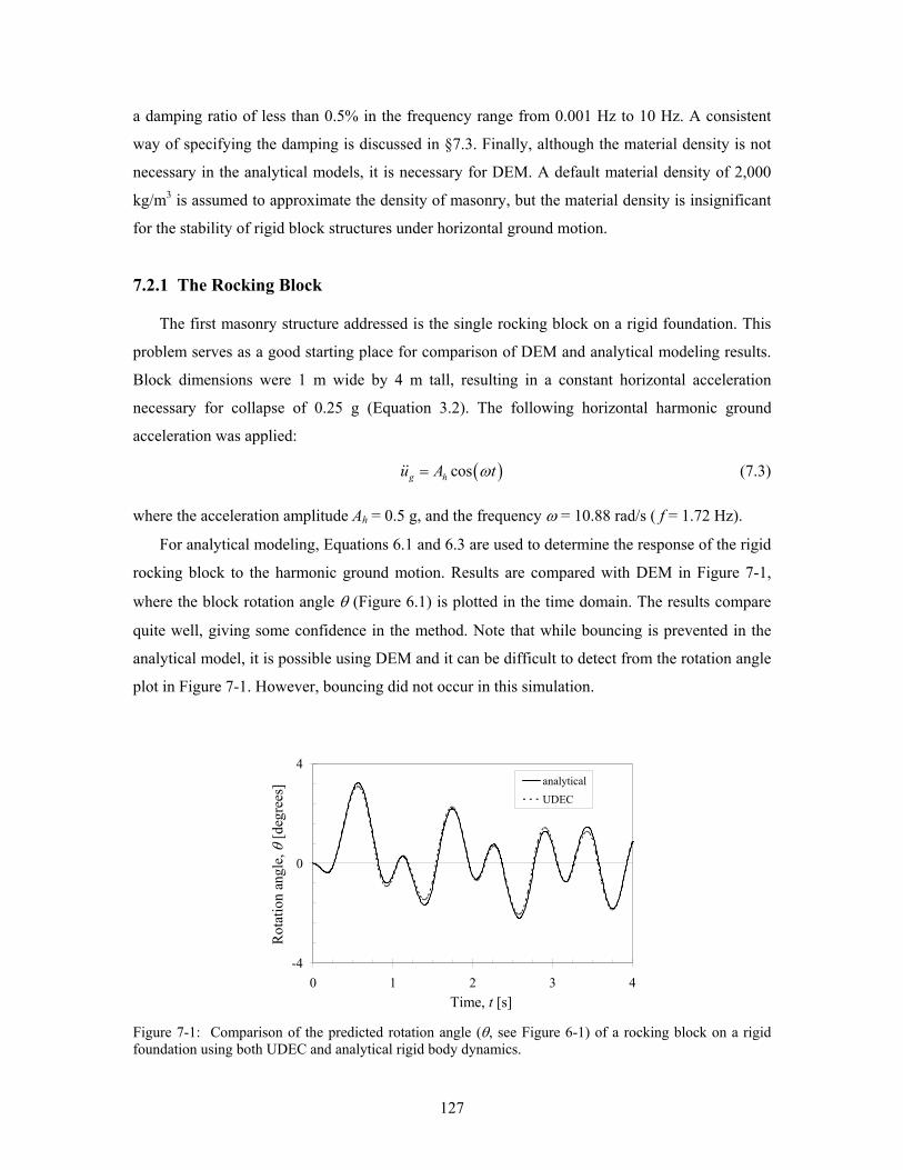
127

a damping ratio of less than 0.5% in the frequency range from 0.001 Hz to 10 Hz. A consistent

way of specifying the damping is discussed in §7.3. Finally, although the material density is not

necessary in the analytical models, it is necessary for DEM. A default material density of 2,000

kg/m3 is assumed to approximate the density of masonry, but the material density is insignificant

for the stability of rigid block structures under horizontal ground motion.


The first masonry structure addressed is the single rocking block on a rigid foundation. This

problem serves as a good starting place for comparison of DEM and analytical modeling results.

Block dimensions were 1 m wide by 4 m tall, resulting in a constant horizontal acceleration

necessary for collapse of 0.25 g (Equation 3.2). The following horizontal harmonic ground

acceleration was applied:

( )cos=g hu A tω (7.3)

where the acceleration amplitude Ah = 0.5 g, and the frequency ω = 10.88 rad/s ( f = 1.72 Hz).

For analytical modeling, Equations 6.1 and 6.3 are used to determine the response of the rigid

rocking block to the harmonic ground motion. Results are compared with DEM in Figure 7-1,

where the block rotation angle θ (Figure 6.1) is plotted in the time domain. The results compare

quite well, giving some confidence in the method. Note that while bouncing is prevented in the

analytical model, it is possible using DEM and it can be difficult to detect from the rotation angle

plot in Figure 7-1. However, bouncing did not occur in this simulation.

Figure 7-1: Comparison of the predicted rotation angle (θ, see Figure 6-1) of a rocking block on a rigid foundation using both UDEC and analytical rigid body dynamics.

-4

0

4

0 1 2 3 4Time [s]

Ang

le o

f Rot

atio

n [d

egre

es] analytical

UDEC

Rot

atio

n an

gle,

θ [d

egre

es]

Time, t [s]

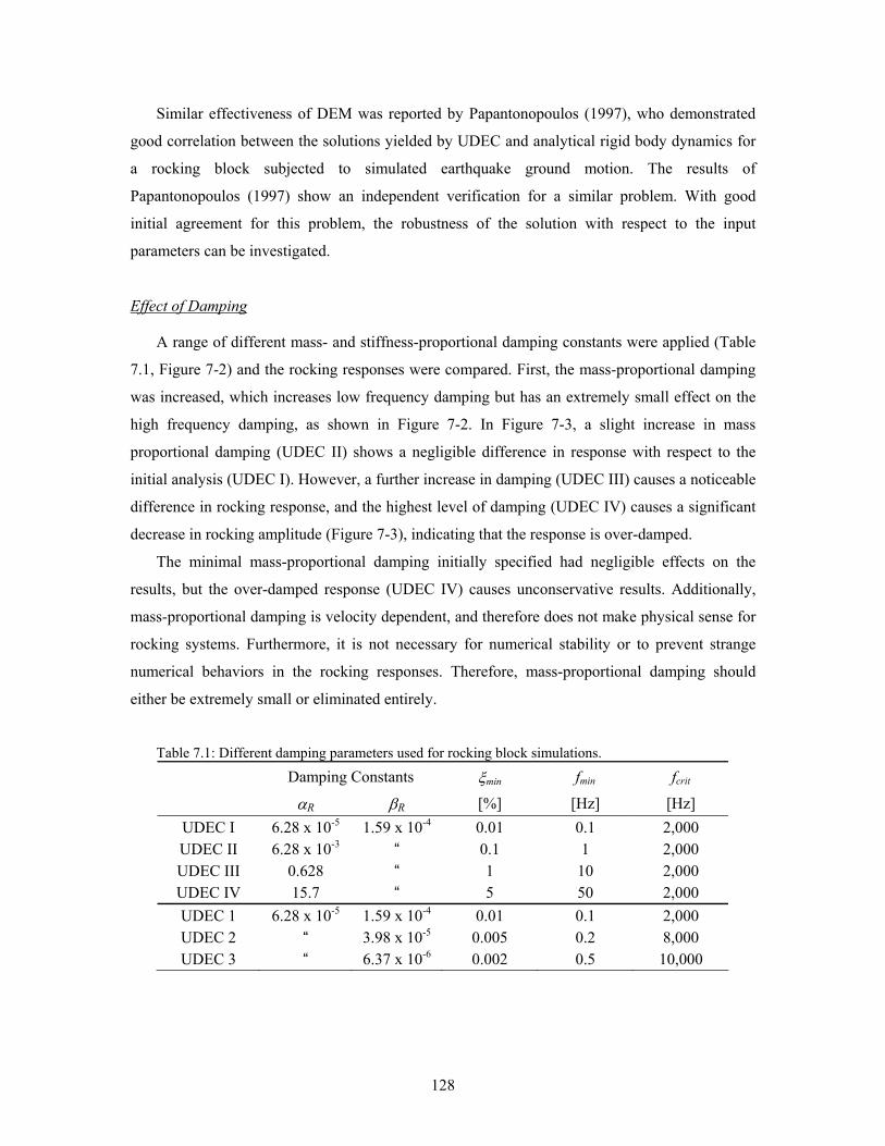
128

Similar effectiveness of DEM was reported by Papantonopoulos (1997), who demonstrated

good correlation between the solutions yielded by UDEC and analytical rigid body dynamics for

a rocking block subjected to simulated earthquake ground motion. The results of

Papantonopoulos (1997) show an independent verification for a similar problem. With good

initial agreement for this problem, the robustness of the solution with respect to the input

parameters can be investigated.

Effect of Damping

A range of different mass- and stiffness-proportional damping constants were applied (Table

7.1, Figure 7-2) and the rocking responses were compared. First, the mass-proportional damping

was increased, which increases low frequency damping but has an extremely small effect on the

high frequency damping, as shown in Figure 7-2. In Figure 7-3, a slight increase in mass

proportional damping (UDEC II) shows a negligible difference in response with respect to the

initial analysis (UDEC I). However, a further increase in damping (UDEC III) causes a noticeable

difference in rocking response, and the highest level of damping (UDEC IV) causes a significant

decrease in rocking amplitude (Figure 7-3), indicating that the response is over-damped.

The minimal mass-proportional damping initially specified had negligible effects on the

results, but the over-damped response (UDEC IV) causes unconservative results. Additionally,

mass-proportional damping is velocity dependent, and therefore does not make physical sense for

rocking systems. Furthermore, it is not necessary for numerical stability or to prevent strange

numerical behaviors in the rocking responses. Therefore, mass-proportional damping should

either be extremely small or eliminated entirely.

Table 7.1: Different damping parameters used for rocking block simulations.

Damping Constants ξmin fmin fcrit

αR βR [%] [Hz] [Hz] UDEC I 6.28 x 10-5 1.59 x 10-4 0.01 0.1 2,000 UDEC II 6.28 x 10-3 “ 0.1 1 2,000 UDEC III 0.628 “ 1 10 2,000 UDEC IV 15.7 “ 5 50 2,000 UDEC 1 6.28 x 10-5 1.59 x 10-4 0.01 0.1 2,000 UDEC 2 “ 3.98 x 10-5 0.005 0.2 8,000 UDEC 3 “ 6.37 x 10-6 0.002 0.5 10,000

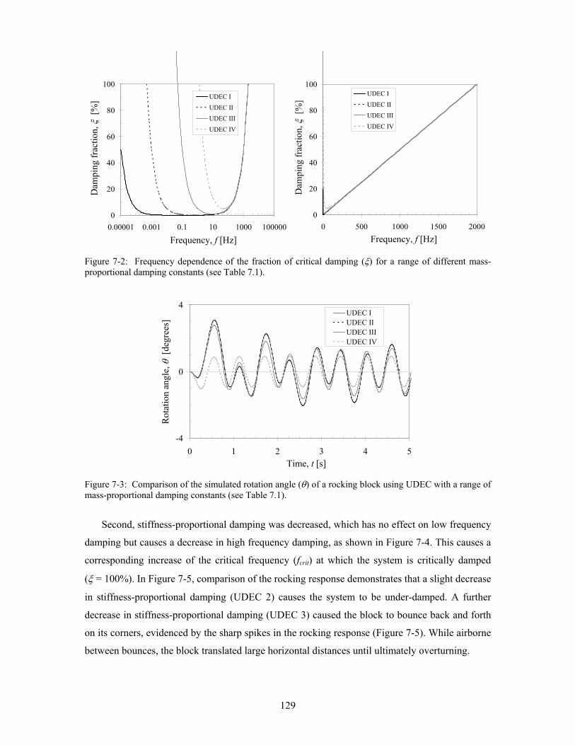
129

Figure 7-2: Frequency dependence of the fraction of critical damping (ξ) for a range of different mass-proportional damping constants (see Table 7.1).

Figure 7-3: Comparison of the simulated rotation angle (θ) of a rocking block using UDEC with a range of mass-proportional damping constants (see Table 7.1).

Second, stiffness-proportional damping was decreased, which has no effect on low frequency

damping but causes a decrease in high frequency damping, as shown in Figure 7-4. This causes a

corresponding increase of the critical frequency (fcrit) at which the system is critically damped

(ξ = 100%). In Figure 7-5, comparison of the rocking response demonstrates that a slight decrease

in stiffness-proportional damping (UDEC 2) causes the system to be under-damped. A further

decrease in stiffness-proportional damping (UDEC 3) caused the block to bounce back and forth

on its corners, evidenced by the sharp spikes in the rocking response (Figure 7-5). While airborne

between bounces, the block translated large horizontal distances until ultimately overturning.

0

20

40

60

80

100

0 500 1000 1500 2000Frequency [Hz]

Dam

ping

Fra

ctio

n [%

]

UDEC I

UDEC II

UDEC III

UDEC IV

0

20

40

60

80

100

0.00001 0.001 0.1 10 1000 100000Frequency [Hz]

Dam

ping

Fra

ctio

n [%

] UDEC I

UDEC II

UDEC III

UDEC IV

Dam

ping

frac

tion,

ξ [

%]

Frequency, f [Hz]

Dam

ping

frac

tion,

ξ [

%]

Frequency, f [Hz]

-4

0

4

0 1 2 3 4 5Time [s]

Rot

atio

n A

ngle

[deg

rees

]

UDEC IUDEC IIUDEC IIIUDEC IV

Rot

atio

n an

gle,

θ [

degr

ees]

Time, t [s]

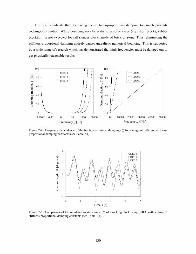
130

The results indicate that decreasing the stiffness-proportional damping too much prevents

rocking-only motion. While bouncing may be realistic in some cases (e.g. short blocks, rubber

blocks), it is not expected for tall slender blocks made of brick or stone. Thus, eliminating the

stiffness-proportional damping entirely causes unrealistic numerical bouncing. This is supported

by a wide range of research which has demonstrated that high-frequencies must be damped out to

get physically reasonable results.

Figure 7-4: Frequency dependence of the fraction of critical damping (ξ) for a range of different stiffness-proportional damping constants (see Table 7.1).

Figure 7-5: Comparison of the simulated rotation angle (θ) of a rocking block using UDEC with a range of stiffness-proportional damping constants (see Table 7.1).

0

20

40

60

80

100

0.00001 0.001 0.1 10 1000 100000Frequency [Hz]

Dam

ping

Fra

ctio

n [%

]

UDEC 1

UDEC 2

UDEC 3

0

20

40

60

80

100

0 10000 20000 30000 40000 50000Frequency [Hz]

Dam

ping

Fra

ctio

n [%

]

UDEC 1

UDEC 2

UDEC 3

Dam

ping

frac

tion,

ξ [

%]

Frequency, f [Hz]

Dam

ping

frac

tion,

ξ [

%]

Frequency, f [Hz]

-4

0

4

0 1 2 3 4 5Time [s]

Rot

atio

n A

ngle

[deg

rees

]

UDEC 1UDEC 2UDEC 3

Rot

atio

n an

gle,

θ [

degr

ees]

Time, t [s]

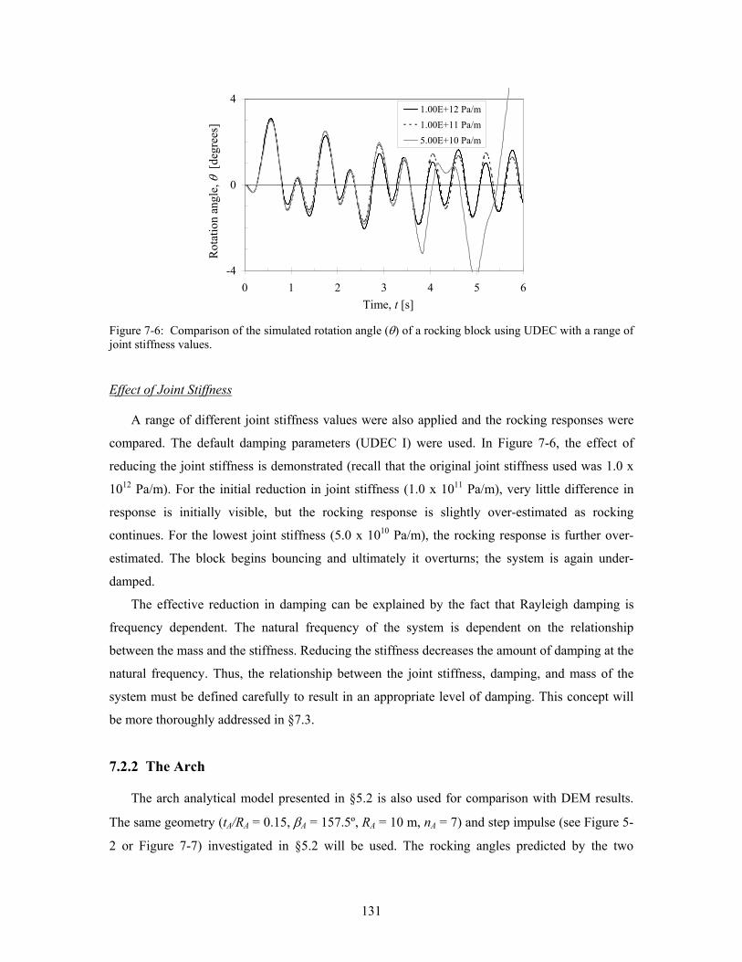
131

Figure 7-6: Comparison of the simulated rotation angle (θ) of a rocking block using UDEC with a range of joint stiffness values.

Effect of Joint Stiffness

A range of different joint stiffness values were also applied and the rocking responses were

compared. The default damping parameters (UDEC I) were used. In Figure 7-6, the effect of

reducing the joint stiffness is demonstrated (recall that the original joint stiffness used was 1.0 x

1012 Pa/m). For the initial reduction in joint stiffness (1.0 x 1011 Pa/m), very little difference in

response is initially visible, but the rocking response is slightly over-estimated as rocking

continues. For the lowest joint stiffness (5.0 x 1010 Pa/m), the rocking response is further over-

estimated. The block begins bouncing and ultimately it overturns; the system is again under-

damped.

The effective reduction in damping can be explained by the fact that Rayleigh damping is

frequency dependent. The natural frequency of the system is dependent on the relationship

between the mass and the stiffness. Reducing the stiffness decreases the amount of damping at the

natural frequency. Thus, the relationship between the joint stiffness, damping, and mass of the

system must be defined carefully to result in an appropriate level of damping. This concept will

be more thoroughly addressed in §7.3.

7.2.2 The Arch

The arch analytical model presented in §5.2 is also used for comparison with DEM results.

The same geometry (tA/RA = 0.15, βA = 157.5º, RA = 10 m, nA = 7) and step impulse (see Figure 5-

2 or Figure 7-7) investigated in §5.2 will be used. The rocking angles predicted by the two

-4

0

4

0 1 2 3 4 5 6Time [s]

Rot

atio

n A

ngle

[deg

rees

]

1.00E+12 Pa/m1.00E+11 Pa/m5.00E+10 Pa/m

Rot

atio

n an

gle,

θ [

degr

ees]

Time, t [s]

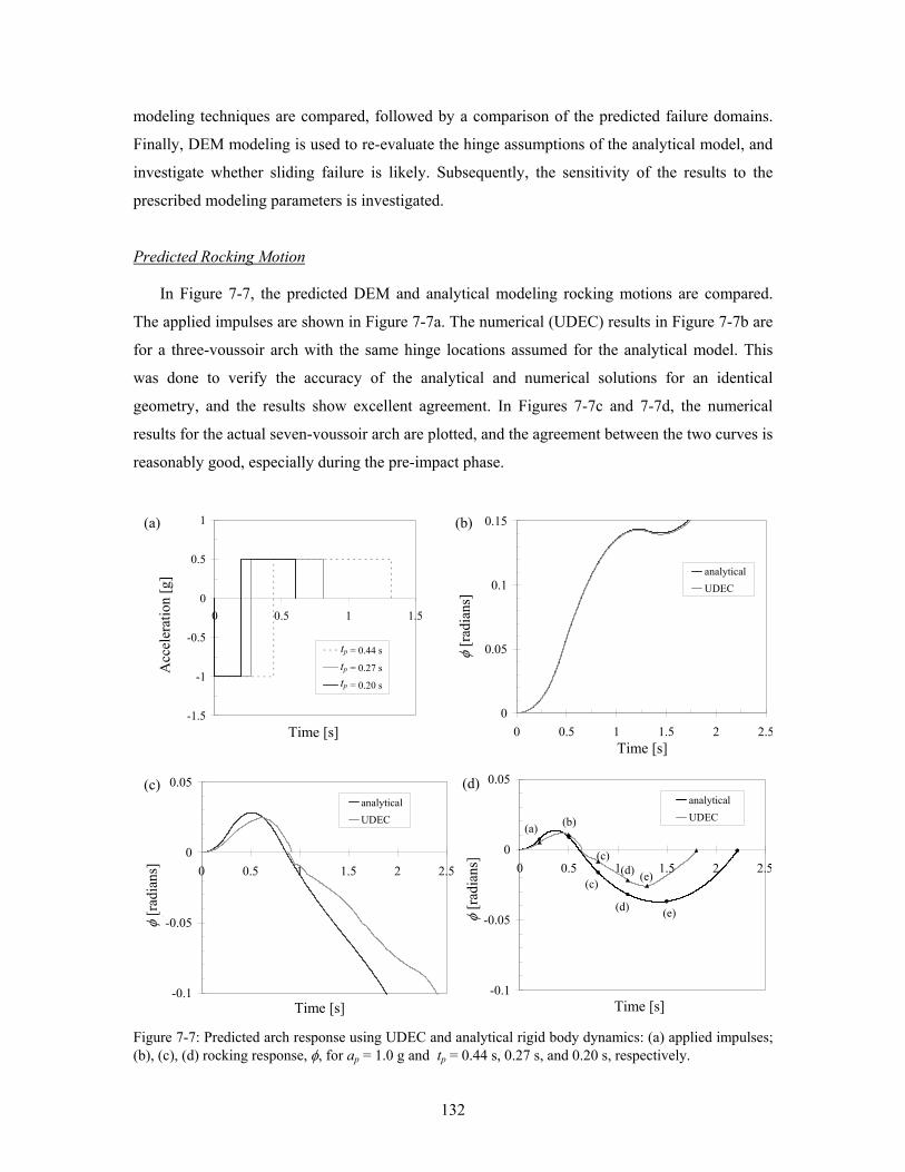
132

modeling techniques are compared, followed by a comparison of the predicted failure domains.

Finally, DEM modeling is used to re-evaluate the hinge assumptions of the analytical model, and

investigate whether sliding failure is likely. Subsequently, the sensitivity of the results to the

prescribed modeling parameters is investigated.

Predicted Rocking Motion

In Figure 7-7, the predicted DEM and analytical modeling rocking motions are compared.

The applied impulses are shown in Figure 7-7a. The numerical (UDEC) results in Figure 7-7b are

for a three-voussoir arch with the same hinge locations assumed for the analytical model. This

was done to verify the accuracy of the analytical and numerical solutions for an identical

geometry, and the results show excellent agreement. In Figures 7-7c and 7-7d, the numerical

results for the actual seven-voussoir arch are plotted, and the agreement between the two curves is

reasonably good, especially during the pre-impact phase.

Figure 7-7: Predicted arch response using UDEC and analytical rigid body dynamics: (a) applied impulses; (b), (c), (d) rocking response, φ, for ap = 1.0 g and tp = 0.44 s, 0.27 s, and 0.20 s, respectively.

-0.1

-0.05

0

0.05

0 0.5 1 1.5 2 2.5

Time [s]

φ [

radi

ans]

analyticalUDEC

0

0.05

0.1

0.15

0 0.5 1 1.5 2 2.5Time [s]

φ [

radi

ans]

analyticalUDEC

-1.5

-1

-0.5

0

0.5

1

0 0.5 1 1.5

Time [s]

Acc

eler

atio

n [g

]

tp = 0.44 s

tp = 0.27 s

tp = 0.20 s

(a)

tp tp tp

(b)

(c) (d)

φ [r

adia

ns]

Time [s]

Acc

eler

atio

n [g

]

Time [s]

φ [r

adia

ns]

-0.1

-0.05

0

0.05

0 0.5 1 1.5 2 2.5

Time [s]

φ [

radi

ans]

analyticalUDEC(b)(a)

(d) (e)

(c)

(c)(d) (e)

φ [r

adia

ns]

Time [s] Time [s]

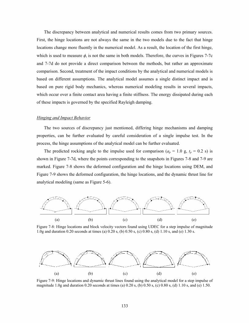
133

The discrepancy between analytical and numerical results comes from two primary sources.

First, the hinge locations are not always the same in the two models due to the fact that hinge

locations change more fluently in the numerical model. As a result, the location of the first hinge,

which is used to measure φ, is not the same in both models. Therefore, the curves in Figures 7-7c

and 7-7d do not provide a direct comparison between the methods, but rather an approximate

comparison. Second, treatment of the impact conditions by the analytical and numerical models is

based on different assumptions. The analytical model assumes a single distinct impact and is

based on pure rigid body mechanics, whereas numerical modeling results in several impacts,

which occur over a finite contact area having a finite stiffness. The energy dissipated during each

of these impacts is governed by the specified Rayleigh damping.

Hinging and Impact Behavior

The two sources of discrepancy just mentioned, differing hinge mechanisms and damping

properties, can be further evaluated by careful consideration of a single impulse test. In the

process, the hinge assumptions of the analytical model can be further evaluated.

The predicted rocking angle to the impulse used for comparison (ap = 1.0 g, tp = 0.2 s) is

shown in Figure 7-7d, where the points corresponding to the snapshots in Figures 7-8 and 7-9 are

marked. Figure 7-8 shows the deformed configuration and the hinge locations using DEM, and

Figure 7-9 shows the deformed configuration, the hinge locations, and the dynamic thrust line for

analytical modeling (same as Figure 5-6).

Figure 7-8: Hinge locations and block velocity vectors found using UDEC for a step impulse of magnitude 1.0g and duration 0.20 seconds at times (a) 0.20 s, (b) 0.50 s, (c) 0.80 s, (d) 1.10 s, and (e) 1.30 s.

Figure 7-9: Hinge locations and dynamic thrust lines found using the analytical model for a step impulse of magnitude 1.0g and duration 0.20 seconds at times (a) 0.20 s, (b) 0.50 s, (c) 0.80 s, (d) 1.10 s, and (e) 1.50.

(a) (b) (c) (d) (e)

(a) (b) (c) (d) (e)

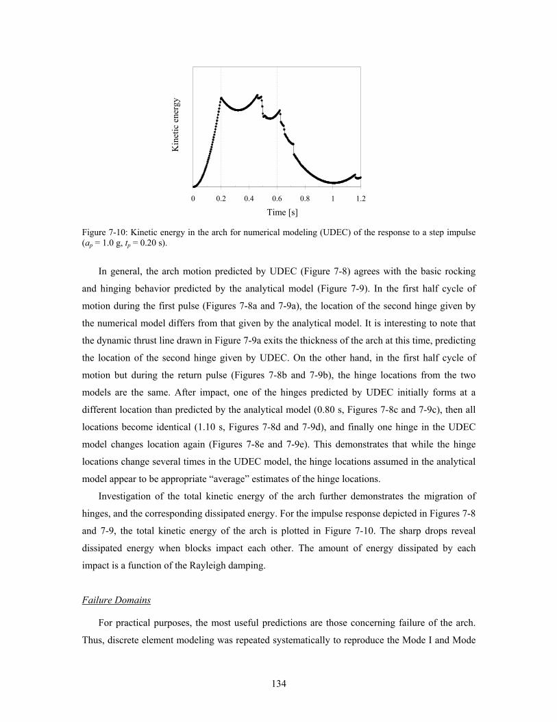
134

Figure 7-10: Kinetic energy in the arch for numerical modeling (UDEC) of the response to a step impulse (ap = 1.0 g, tp = 0.20 s).

In general, the arch motion predicted by UDEC (Figure 7-8) agrees with the basic rocking

and hinging behavior predicted by the analytical model (Figure 7-9). In the first half cycle of

motion during the first pulse (Figures 7-8a and 7-9a), the location of the second hinge given by

the numerical model differs from that given by the analytical model. It is interesting to note that

the dynamic thrust line drawn in Figure 7-9a exits the thickness of the arch at this time, predicting

the location of the second hinge given by UDEC. On the other hand, in the first half cycle of

motion but during the return pulse (Figures 7-8b and 7-9b), the hinge locations from the two

models are the same. After impact, one of the hinges predicted by UDEC initially forms at a

different location than predicted by the analytical model (0.80 s, Figures 7-8c and 7-9c), then all

locations become identical (1.10 s, Figures 7-8d and 7-9d), and finally one hinge in the UDEC

model changes location again (Figures 7-8e and 7-9e). This demonstrates that while the hinge

locations change several times in the UDEC model, the hinge locations assumed in the analytical

model appear to be appropriate “average” estimates of the hinge locations.

Investigation of the total kinetic energy of the arch further demonstrates the migration of

hinges, and the corresponding dissipated energy. For the impulse response depicted in Figures 7-8

and 7-9, the total kinetic energy of the arch is plotted in Figure 7-10. The sharp drops reveal

dissipated energy when blocks impact each other. The amount of energy dissipated by each

impact is a function of the Rayleigh damping.

Failure Domains

For practical purposes, the most useful predictions are those concerning failure of the arch.

Thus, discrete element modeling was repeated systematically to reproduce the Mode I and Mode

Kin

etic

ene

rgy

Time [s] 0 0.2 0.4 0.6 0.8 1 1.2

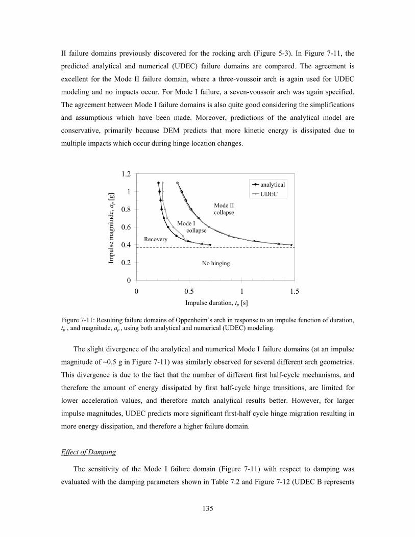
135

II failure domains previously discovered for the rocking arch (Figure 5-3). In Figure 7-11, the

predicted analytical and numerical (UDEC) failure domains are compared. The agreement is

excellent for the Mode II failure domain, where a three-voussoir arch is again used for UDEC

modeling and no impacts occur. For Mode I failure, a seven-voussoir arch was again specified.

The agreement between Mode I failure domains is also quite good considering the simplifications

and assumptions which have been made. Moreover, predictions of the analytical model are

conservative, primarily because DEM predicts that more kinetic energy is dissipated due to

multiple impacts which occur during hinge location changes.

Figure 7-11: Resulting failure domains of Oppenheim’s arch in response to an impulse function of duration, tp , and magnitude, ap , using both analytical and numerical (UDEC) modeling.

The slight divergence of the analytical and numerical Mode I failure domains (at an impulse

magnitude of ~0.5 g in Figure 7-11) was similarly observed for several different arch geometries.

This divergence is due to the fact that the number of different first half-cycle mechanisms, and

therefore the amount of energy dissipated by first half-cycle hinge transitions, are limited for

lower acceleration values, and therefore match analytical results better. However, for larger

impulse magnitudes, UDEC predicts more significant first-half cycle hinge migration resulting in

more energy dissipation, and therefore a higher failure domain.

Effect of Damping

The sensitivity of the Mode I failure domain (Figure 7-11) with respect to damping was

evaluated with the damping parameters shown in Table 7.2 and Figure 7-12 (UDEC B represents

0

0.2

0.4

0.6

0.8

1

1.2

0 0.5 1 1.5

Impulse duration, td [s]

Impu

lse

mag

nitu

de, a

[g] analytical

UDEC

Mode I collapse

Mode II collapse

Recovery

No hinging


Impu

lse

mag

nitu

de, a

p [g]

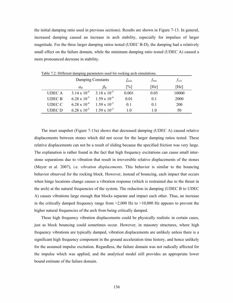
136

the initial damping ratio used in previous sections). Results are shown in Figure 7-13. In general,

increased damping caused an increase in arch stability, especially for impulses of larger

magnitude. For the three larger damping ratios tested (UDEC B-D), the damping had a relatively

small effect on the failure domain, while the minimum damping ratio tested (UDEC A) caused a

more pronounced decrease in stability.

Table 7.2: Different damping parameters used for rocking arch simulations.

Damping Constants ξmin fmin fcrit

αR βR [%] [Hz] [Hz] UDEC A 3.14 x 10-6 3.18 x 10-5 0.001 0.05 10000 UDEC B 6.28 x 10-5 1.59 x 10-4 0.01 0.1 2000 UDEC C 6.28 x 10-4 1.59 x 10-3 0.1 0.1 200 UDEC D 6.28 x 10-2 1.59 x 10-3 1.0 1.0 50

The inset snapshot (Figure 7-13a) shows that decreased damping (UDEC A) caused relative

displacements between stones which did not occur for the larger damping ratios tested. These

relative displacements can not be a result of sliding because the specified friction was very large.

The explanation is rather found in the fact that high frequency excitations can cause small inter-

stone separations due to vibration that result in irreversible relative displacements of the stones

(Meyer et al. 2007), i.e. vibration displacements. This behavior is similar to the bouncing

behavior observed for the rocking block. However, instead of bouncing, each impact that occurs

when hinge locations change causes a vibration response (which is restrained due to the thrust in

the arch) at the natural frequencies of the system. The reduction in damping (UDEC B to UDEC

A) causes vibrations large enough that blocks separate and impact each other. Thus, an increase

in the critically damped frequency range from >2,000 Hz to >10,000 Hz appears to prevent the

higher natural frequencies of the arch from being critically damped.

These high frequency vibration displacements could be physically realistic in certain cases,

just as block bouncing could sometimes occur. However, in masonry structures, where high

frequency vibrations are typically damped, vibration displacements are unlikely unless there is a

significant high frequency component in the ground acceleration time history, and hence unlikely

for the assumed impulse excitation. Regardless, the failure domain was not radically affected for

the impulse which was applied, and the analytical model still provides an appropriate lower

bound estimate of the failure domain.

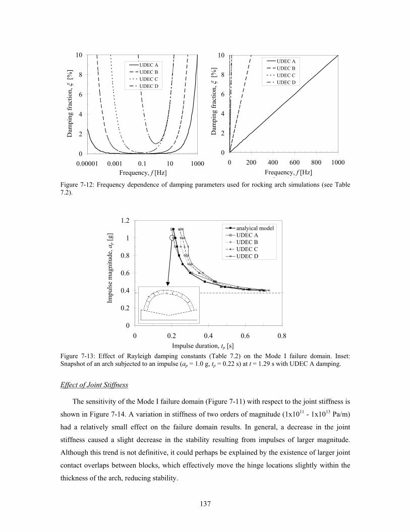
137

Figure 7-12: Frequency dependence of damping parameters used for rocking arch simulations (see Table 7.2).

Figure 7-13: Effect of Rayleigh damping constants (Table 7.2) on the Mode I failure domain. Inset: Snapshot of an arch subjected to an impulse (ap = 1.0 g, tp = 0.22 s) at t = 1.29 s with UDEC A damping.

Effect of Joint Stiffness

The sensitivity of the Mode I failure domain (Figure 7-11) with respect to the joint stiffness is

shown in Figure 7-14. A variation in stiffness of two orders of magnitude (1x1011 - 1x1013 Pa/m)

had a relatively small effect on the failure domain results. In general, a decrease in the joint

stiffness caused a slight decrease in the stability resulting from impulses of larger magnitude.

Although this trend is not definitive, it could perhaps be explained by the existence of larger joint

contact overlaps between blocks, which effectively move the hinge locations slightly within the

thickness of the arch, reducing stability.

0

2

4

6

8

10

0.00001 0.001 0.1 10 1000Frequency [Hz]

Dam

ping

Fra

ctio

n [%

] UDEC AUDEC BUDEC CUDEC D

0

2

4

6

8

10

0 200 400 600 800 1000

Frequency [Hz]

Dam

ping

Fra

ctio

n [%

]

UDEC AUDEC BUDEC CUDEC D

Dam

ping

frac

tion,

ξ [

%]

Frequency, f [Hz]

Dam

ping

frac

tion,

ξ [

%]

Frequency, f [Hz]

0

0.2

0.4

0.6

0.8

1

1.2

0 0.2 0.4 0.6 0.8Impulse duration, tp [s]

Impu

lse

mag

nitu

de, a

[*g]

analyical modelUDEC AUDEC BUDEC CUDEC D


Impu

lse

mag

nitu

de, a

p [g]

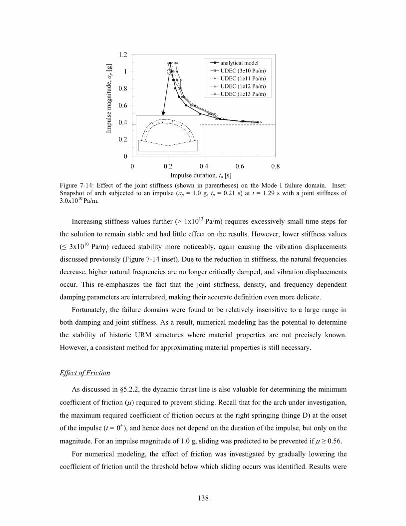
138

Figure 7-14: Effect of the joint stiffness (shown in parentheses) on the Mode I failure domain. Inset: Snapshot of arch subjected to an impulse (ap = 1.0 g, tp = 0.21 s) at t = 1.29 s with a joint stiffness of 3.0x1010 Pa/m.

Increasing stiffness values further (> 1x1013 Pa/m) requires excessively small time steps for

the solution to remain stable and had little effect on the results. However, lower stiffness values

(≤ 3x1010 Pa/m) reduced stability more noticeably, again causing the vibration displacements

discussed previously (Figure 7-14 inset). Due to the reduction in stiffness, the natural frequencies

decrease, higher natural frequencies are no longer critically damped, and vibration displacements

occur. This re-emphasizes the fact that the joint stiffness, density, and frequency dependent

damping parameters are interrelated, making their accurate definition even more delicate.

Fortunately, the failure domains were found to be relatively insensitive to a large range in

both damping and joint stiffness. As a result, numerical modeling has the potential to determine

the stability of historic URM structures where material properties are not precisely known.

However, a consistent method for approximating material properties is still necessary.

Effect of Friction

As discussed in §5.2.2, the dynamic thrust line is also valuable for determining the minimum

coefficient of friction (μ) required to prevent sliding. Recall that for the arch under investigation,

the maximum required coefficient of friction occurs at the right springing (hinge D) at the onset

of the impulse (t = 0+), and hence does not depend on the duration of the impulse, but only on the

magnitude. For an impulse magnitude of 1.0 g, sliding was predicted to be prevented if μ ≥ 0.56.

For numerical modeling, the effect of friction was investigated by gradually lowering the

coefficient of friction until the threshold below which sliding occurs was identified. Results were

0

0.2

0.4

0.6

0.8

1

1.2

0 0.2 0.4 0.6 0.8Impulse duration, tp [s]

Impu

lse

mag

nitu

de, a

[*g]

analytical modelUDEC (3e10 Pa/m)UDEC (1e11 Pa/m)UDEC (1e12 Pa/m)UDEC (1e13 Pa/m)


Impu

lse

mag

nitu

de, a

p [g]

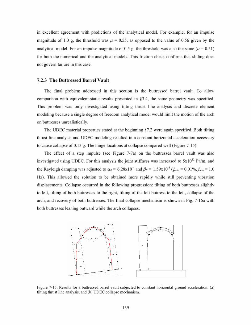
139

in excellent agreement with predictions of the analytical model. For example, for an impulse

magnitude of 1.0 g, the threshold was μ = 0.55, as opposed to the value of 0.56 given by the

analytical model. For an impulse magnitude of 0.5 g, the threshold was also the same (μ = 0.51)

for both the numerical and the analytical models. This friction check confirms that sliding does

not govern failure in this case.

7.2.3 The Buttressed Barrel Vault

The final problem addressed in this section is the buttressed barrel vault. To allow

comparison with equivalent-static results presented in §3.4, the same geometry was specified.

This problem was only investigated using tilting thrust line analysis and discrete element

modeling because a single degree of freedom analytical model would limit the motion of the arch

on buttresses unrealistically.

The UDEC material properties stated at the beginning §7.2 were again specified. Both tilting

thrust line analysis and UDEC modeling resulted in a constant horizontal acceleration necessary

to cause collapse of 0.13 g. The hinge locations at collapse compared well (Figure 7-15).

The effect of a step impulse (see Figure 7-7a) on the buttresses barrel vault was also

investigated using UDEC. For this analysis the joint stiffness was increased to 5x1012 Pa/m, and

the Rayleigh damping was adjusted to αR = 6.28x10-4 and βR = 1.59x10-5 (ξmin = 0.01%, fmin = 1.0

Hz). This allowed the solution to be obtained more rapidly while still preventing vibration

displacements. Collapse occurred in the following progression: tilting of both buttresses slightly

to left, tilting of both buttresses to the right, tilting of the left buttress to the left, collapse of the

arch, and recovery of both buttresses. The final collapse mechanism is shown in Fig. 7-16a with

both buttresses leaning outward while the arch collapses.

Figure 7-15: Results for a buttressed barrel vault subjected to constant horizontal ground acceleration: (a) tilting thrust line analysis, and (b) UDEC collapse mechanism.

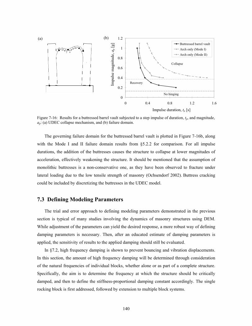
140

Figure 7-16: Results for a buttressed barrel vault subjected to a step impulse of duration, tp, and magnitude, ap: (a) UDEC collapse mechanism, and (b) failure domain.

The governing failure domain for the buttressed barrel vault is plotted in Figure 7-16b, along

with the Mode I and II failure domain results from §5.2.2 for comparison. For all impulse

durations, the addition of the buttresses causes the structure to collapse at lower magnitudes of

acceleration, effectively weakening the structure. It should be mentioned that the assumption of

monolithic buttresses is a non-conservative one, as they have been observed to fracture under

lateral loading due to the low tensile strength of masonry (Ochsendorf 2002). Buttress cracking

could be included by discretizing the buttresses in the UDEC model.

7.3 Defining Modeling Parameters

The trial and error approach to defining modeling parameters demonstrated in the previous

section is typical of many studies involving the dynamics of masonry structures using DEM.

While adjustment of the parameters can yield the desired response, a more robust way of defining

damping parameters is necessary. Then, after an educated estimate of damping parameters is

applied, the sensitivity of results to the applied damping should still be evaluated.

In §7.2, high frequency damping is shown to prevent bouncing and vibration displacements.

In this section, the amount of high frequency damping will be determined through consideration

of the natural frequencies of individual blocks, whether alone or as part of a complete structure.

Specifically, the aim is to determine the frequency at which the structure should be critically

damped, and then to define the stiffness-proportional damping constant accordingly. The single

rocking block is first addressed, followed by extension to multiple block systems.

0

0.2

0.4

0.6

0.8

1

1.2

0 0.4 0.8 1.2 1.6Impulse duration [s]

Impu

lse

acce

lera

tion,

*g

Buttressed barrel vaultArch only (Mode I)Arch only (Mode II)

Impulse duration, tp [s] Im

puls

e m

agni

tude

, ap [

g]

Collapse

Recovery

No hinging

(b) (a)

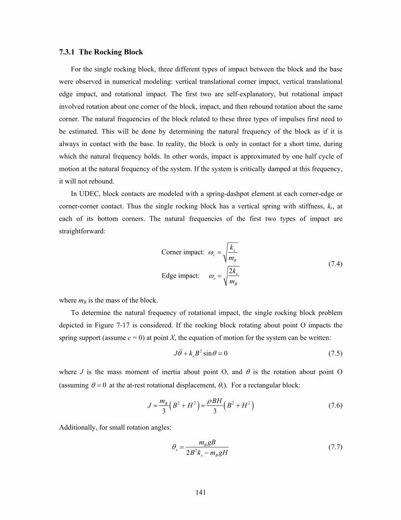
141


For the single rocking block, three different types of impact between the block and the base

were observed in numerical modeling: vertical translational corner impact, vertical translational

edge impact, and rotational impact. The first two are self-explanatory, but rotational impact

involved rotation about one corner of the block, impact, and then rebound rotation about the same

corner. The natural frequencies of the block related to these three types of impulses first need to

be estimated. This will be done by determining the natural frequency of the block as if it is

always in contact with the base. In reality, the block is only in contact for a short time, during

which the natural frequency holds. In other words, impact is approximated by one half cycle of

motion at the natural frequency of the system. If the system is critically damped at this frequency,

it will not rebound.

In UDEC, block contacts are modeled with a spring-dashpot element at each corner-edge or

corner-corner contact. Thus the single rocking block has a vertical spring with stiffness, ks, at

each of its bottom corners. The natural frequencies of the first two types of impact are

straightforward:

Corner impact:

2Edge impact:

=

=

sc

B

se

B

km

km

ω

ω

(7.4)

where mB is the mass of the block.

To determine the natural frequency of rotational impact, the single rocking block problem

depicted in Figure 7-17 is considered. If the rocking block rotating about point O impacts the

spring support (assume c = 0) at point X, the equation of motion for the system can be written:

2 sin 0+ =sJ k Bθ θ (7.5)

where J is the mass moment of inertia about point O, and θ is the rotation about point O

(assuming 0=θ at the at-rest rotational displacement, θs). For a rectangular block:

( ) ( )2 2 2 2

3 3= + = +Bm BHJ B H B Hρ (7.6)

Additionally, for small rotation angles:

22=

−B

ss B

m gBB k m gH

θ (7.7)

142

Note that for a very stiff spring, mgh is negligible with respect to 2B2ks, and the at-rest rotational

displacement reduces to:

2

= Bs

s

m gBk

θ (7.8)

From Equations 7.5 and 7.6, the natural frequency associated with rocking impact is determined:

( ) ( )

2 2

2 2 2 2

3 3= = =

+ +s s s

rB

k B k B k BJ m B H H B H

ωρ

(7.9)

Figure 7-17: Definition of the rotational impact problem.

Joint Stiffness

To calculate the impact frequencies, the joint stiffness needs to be defined. For rigid blocks, it

is assumed that the deformation is concentrated in the joints. The joint stiffness, kj, is then defined

using the material properties of the blocks:

=jEAkL

(7.10)

where E is the modulus of elasticity of the masonry blocks, A is the area of contact between the

blocks, and L is the length of rigid material represented in the direction perpendicular to the joint,

as mentioned in §7.1. For the rocking block in question, this reduces to:

=jEBkH

(7.11)

H

x

y

O

B

c ks

X

θ

143

The joint stiffness has been determined but must be translated into a spring stiffness, ks.

Since the stiffness is lumped to springs at the corners of the blocks, and the spring stiffness is

defined as:

2

2 2= =j

s

k B EBkH

(7.12)

The impact frequencies of the system (Equations 7.4 and 7.9) are:

( )

2

2

3 4 3

2 2 2

Corner impact: 2 2

Edge impact:

3Rotational impact: 2 2 2

= =

= =

= = =+

jc

B B

je

B B

jr

k B EBm Hm

k B EBm Hm

k B EB EBJ HJ H B H

ω

ω

ωρ

(7.13)

Selection of the Critical Frequency

To select which impact frequency should be specified as the critical frequency, it is useful to

compare the rotational impact (Equation 7.9) and bouncing impact (Equation 7.4) frequencies:

222 11

;3 3

⎛ ⎞⎛ ⎞⎛ ⎞ +⎜ ⎟⎜ ⎟+ ⎜ ⎟ ⎜ ⎟⎝ ⎠⎝ ⎠ ⎝ ⎠= =c e

r r

HHBBω ω

ω ω (7.14)

The relationships in Equation 7.14 are plotted in Figure 7-18. Provided that 2>H B , one

finds that <r cω ω . Likewise, provided that 1 2>H B , one finds that <r eω ω . Thus, provided

that 2>H B :

< <r c eω ω ω (7.15)

Therefore, specifying critical damping (ξ = 100%) at ωr will cause ωc and ωe to be over-

damped (ξ > 100%), and would be least conservative. Alternatively, specifying critical damping

at ωe would cause ωr and ωc to be under-damped ( ξ < 100%), and would be most conservative

but might not ensure that rocking and bouncing do not occur. Either choice is reasonable, but both

extremes should be checked to determine the sensitivity of results.

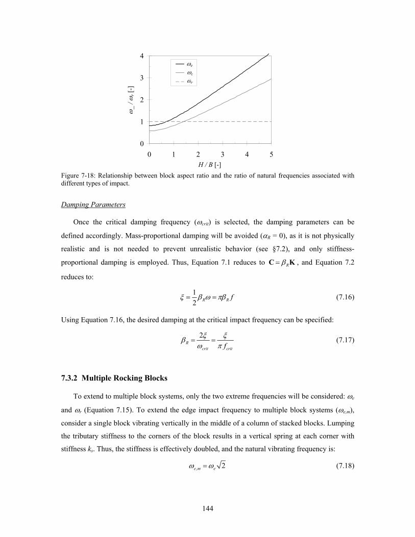
144

Figure 7-18: Relationship between block aspect ratio and the ratio of natural frequencies associated with different types of impact.

Damping Parameters

Once the critical damping frequency (ωcrit) is selected, the damping parameters can be

defined accordingly. Mass-proportional damping will be avoided (αR = 0), as it is not physically

realistic and is not needed to prevent unrealistic behavior (see §7.2), and only stiffness-

proportional damping is employed. Thus, Equation 7.1 reduces to = RβC K , and Equation 7.2

reduces to:

12

= =R R fξ β ω πβ (7.16)

Using Equation 7.16, the desired damping at the critical impact frequency can be specified:

2= =R

crit critfξ ξβ

ω π (7.17)

7.3.2 Multiple Rocking Blocks

To extend to multiple block systems, only the two extreme frequencies will be considered: ωe

and ωr (Equation 7.15). To extend the edge impact frequency to multiple block systems (ωe,m),

consider a single block vibrating vertically in the middle of a column of stacked blocks. Lumping

the tributary stiffness to the corners of the block results in a vertical spring at each corner with

stiffness ks. Thus, the stiffness is effectively doubled, and the natural vibrating frequency is:

, 2=e m eω ω (7.18)

0

1

2

3

4

0 1 2 3 4 5h / b

ti,r /

ti,b

wewcwr

ω_

/ ωr [

-]

H / B [-]

ωe ωc ωr

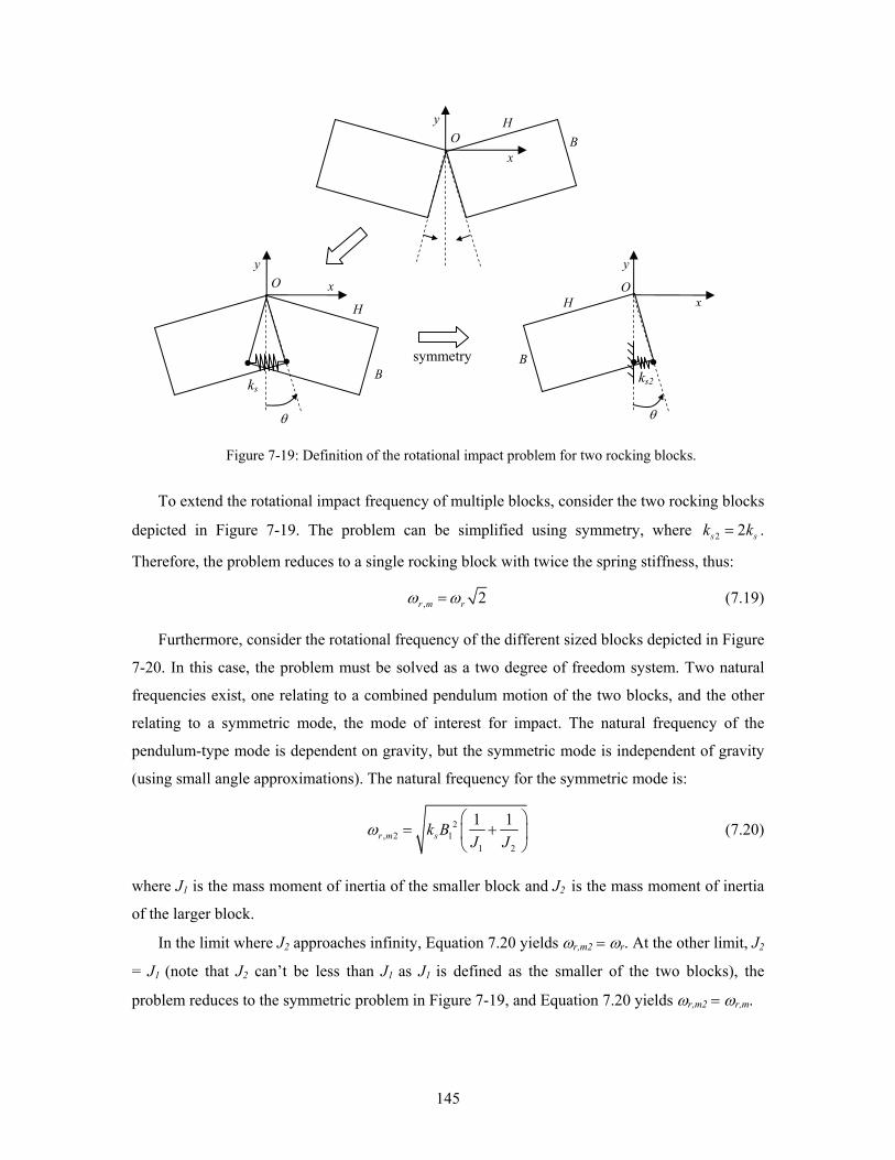
145

Figure 7-19: Definition of the rotational impact problem for two rocking blocks.

To extend the rotational impact frequency of multiple blocks, consider the two rocking blocks

depicted in Figure 7-19. The problem can be simplified using symmetry, where 2 2=s sk k .

Therefore, the problem reduces to a single rocking block with twice the spring stiffness, thus:

, 2=r m rω ω (7.19)

Furthermore, consider the rotational frequency of the different sized blocks depicted in Figure

7-20. In this case, the problem must be solved as a two degree of freedom system. Two natural

frequencies exist, one relating to a combined pendulum motion of the two blocks, and the other

relating to a symmetric mode, the mode of interest for impact. The natural frequency of the

pendulum-type mode is dependent on gravity, but the symmetric mode is independent of gravity

(using small angle approximations). The natural frequency for the symmetric mode is:

2, 2 1

1 2

1 1⎛ ⎞= +⎜ ⎟

⎝ ⎠r m sk B

J Jω (7.20)

where J1 is the mass moment of inertia of the smaller block and J2 is the mass moment of inertia

of the larger block.

In the limit where J2 approaches infinity, Equation 7.20 yields ωr,m2 = ωr. At the other limit, J2

= J1 (note that J2 can’t be less than J1 as J1 is defined as the smaller of the two blocks), the

problem reduces to the symmetric problem in Figure 7-19, and Equation 7.20 yields ωr,m2 = ωr,m.

xO

ks

θ

y

H

B

xO

ks2

θ

y

H

B

xO B

y H

symmetry

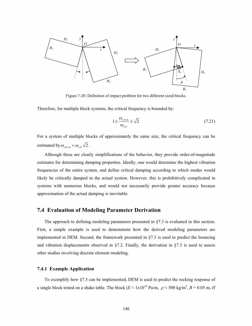
146

Figure 7-20: Definition of impact problem for two different sized blocks.

Therefore, for multiple block systems, the critical frequency is bounded by:

,1 2≤ ≤crit m

crit

ωω

(7.21)

For a system of multiple blocks of approximately the same size, the critical frequency can be

estimated by , 2=crit m critω ω .

Although these are clearly simplifications of the behavior, they provide order-of-magnitude

estimates for determining damping properties. Ideally, one would determine the highest vibration

frequencies of the entire system, and define critical damping according to which modes would

likely be critically damped in the actual system. However, this is prohibitively complicated in

systems with numerous blocks, and would not necessarily provide greater accuracy because

approximation of the actual damping is inevitable.

7.4 Evaluation of Modeling Parameter Derivation

The approach to defining modeling parameters presented in §7.3 is evaluated in this section.

First, a simple example is used to demonstrate how the derived modeling parameters are

implemented in DEM. Second, the framework presented in §7.3 is used to predict the bouncing

and vibration displacements observed in §7.2. Finally, the derivation in §7.3 is used to assess

other studies involving discrete element modeling.

7.4.1 Example Application

To exemplify how §7.3 can be implemented, DEM is used to predict the rocking response of

a single block tested on a shake table. The block (E ≈ 1x1010 Pa/m, ρ ≈ 500 kg/m3, B = 0.05 m, H

xO

B2

y

H2

H1

B1 xO

ks

θ

y

B2

H2

H1

B1

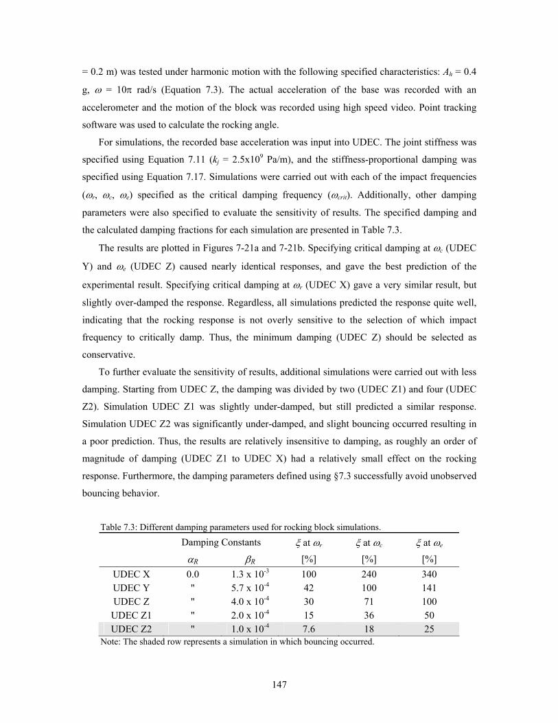
147

= 0.2 m) was tested under harmonic motion with the following specified characteristics: Ah = 0.4

g, ω = 10π rad/s (Equation 7.3). The actual acceleration of the base was recorded with an

accelerometer and the motion of the block was recorded using high speed video. Point tracking

software was used to calculate the rocking angle.

For simulations, the recorded base acceleration was input into UDEC. The joint stiffness was

specified using Equation 7.11 (kj = 2.5x109 Pa/m), and the stiffness-proportional damping was

specified using Equation 7.17. Simulations were carried out with each of the impact frequencies

(ωr, ωc, ωe) specified as the critical damping frequency (ωcrit). Additionally, other damping

parameters were also specified to evaluate the sensitivity of results. The specified damping and

the calculated damping fractions for each simulation are presented in Table 7.3.

The results are plotted in Figures 7-21a and 7-21b. Specifying critical damping at ωc (UDEC

Y) and ωe (UDEC Z) caused nearly identical responses, and gave the best prediction of the

experimental result. Specifying critical damping at ωr (UDEC X) gave a very similar result, but

slightly over-damped the response. Regardless, all simulations predicted the response quite well,

indicating that the rocking response is not overly sensitive to the selection of which impact

frequency to critically damp. Thus, the minimum damping (UDEC Z) should be selected as

conservative.

To further evaluate the sensitivity of results, additional simulations were carried out with less

damping. Starting from UDEC Z, the damping was divided by two (UDEC Z1) and four (UDEC

Z2). Simulation UDEC Z1 was slightly under-damped, but still predicted a similar response.

Simulation UDEC Z2 was significantly under-damped, and slight bouncing occurred resulting in

a poor prediction. Thus, the results are relatively insensitive to damping, as roughly an order of

magnitude of damping (UDEC Z1 to UDEC X) had a relatively small effect on the rocking

response. Furthermore, the damping parameters defined using §7.3 successfully avoid unobserved

bouncing behavior.

Table 7.3: Different damping parameters used for rocking block simulations.

Damping Constants ξ at ωr ξ at ωc ξ at ωe αR βR [%] [%] [%]

UDEC X 0.0 1.3 x 10-3 100 240 340 UDEC Y " 5.7 x 10-4 42 100 141 UDEC Z " 4.0 x 10-4 30 71 100

UDEC Z1 " 2.0 x 10-4 15 36 50 UDEC Z2 " 1.0 x 10-4 7.6 18 25

Note: The shaded row represents a simulation in which bouncing occurred.

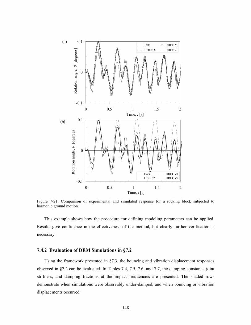
148

Figure 7-21: Comparison of experimental and simulated response for a rocking block subjected to harmonic ground motion.

This example shows how the procedure for defining modeling parameters can be applied.

Results give confidence in the effectiveness of the method, but clearly further verification is

necessary.

7.4.2 Evaluation of DEM Simulations in §7.2

Using the framework presented in §7.3, the bouncing and vibration displacement responses

observed in §7.2 can be evaluated. In Tables 7.4, 7.5, 7.6, and 7.7, the damping constants, joint

stiffness, and damping fractions at the impact frequencies are presented. The shaded rows

demonstrate when simulations were observably under-damped, and when bouncing or vibration

displacements occurred.

-0.1

0

0.1

0 0.5 1 1.5 2Time [s]

Roc

king

ang

le [r

ad]

l

Data UDEC YUDEC X UDEC Z

-0.1

0

0.1

0 0.5 1 1.5 2Time [s]

Roc

king

ang

le [r

ad]

l

Data UDEC Z1UDEC Z UDEC Z2

Rot

atio

n an

gle,

θ [

degr

ees]

Time, t [s]

Time, t [s]

Rot

atio

n an

gle,

θ [

degr

ees]

(a)

(b)

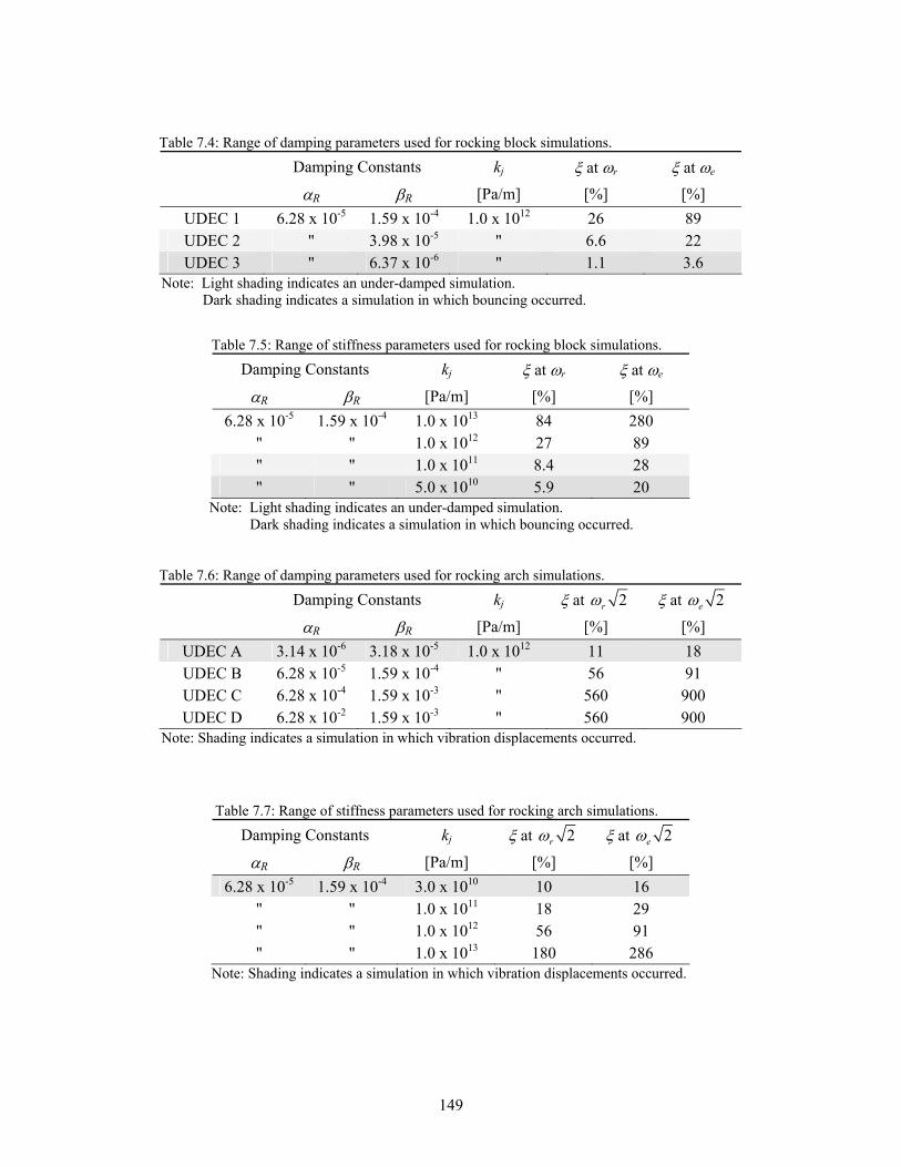
149

Table 7.4: Range of damping parameters used for rocking block simulations.

Damping Constants kj ξ at ωr ξ at ωe αR βR [Pa/m] [%] [%]

UDEC 1 6.28 x 10-5 1.59 x 10-4 1.0 x 1012 26 89 UDEC 2 " 3.98 x 10-5 " 6.6 22 UDEC 3 " 6.37 x 10-6 " 1.1 3.6

Note: Light shading indicates an under-damped simulation. Dark shading indicates a simulation in which bouncing occurred.

Table 7.5: Range of stiffness parameters used for rocking block simulations.

Damping Constants kj ξ at ωr ξ at ωe

αR βR [Pa/m] [%] [%] 6.28 x 10-5 1.59 x 10-4 1.0 x 1013 84 280

" " 1.0 x 1012 27 89 " " 1.0 x 1011 8.4 28 " " 5.0 x 1010 5.9 20

Note: Light shading indicates an under-damped simulation. Dark shading indicates a simulation in which bouncing occurred. Table 7.6: Range of damping parameters used for rocking arch simulations.

Damping Constants kj ξ at 2rω ξ at 2eω

αR βR [Pa/m] [%] [%] UDEC A 3.14 x 10-6 3.18 x 10-5 1.0 x 1012 11 18 UDEC B 6.28 x 10-5 1.59 x 10-4 " 56 91 UDEC C 6.28 x 10-4 1.59 x 10-3 " 560 900 UDEC D 6.28 x 10-2 1.59 x 10-3 " 560 900

Note: Shading indicates a simulation in which vibration displacements occurred.

Table 7.7: Range of stiffness parameters used for rocking arch simulations.

Damping Constants kj ξ at 2rω ξ at 2eω

αR βR [Pa/m] [%] [%] 6.28 x 10-5 1.59 x 10-4 3.0 x 1010 10 16

" " 1.0 x 1011 18 29 " " 1.0 x 1012 56 91 " " 1.0 x 1013 180 286

Note: Shading indicates a simulation in which vibration displacements occurred.

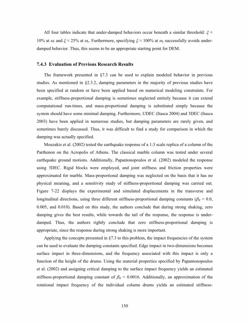
150

All four tables indicate that under-damped behaviors occur beneath a similar threshold: ξ ≈

10% at ωr and ξ ≈ 25% at ωe. Furthermore, specifying ξ ≈ 100% at ωe successfully avoids under-

damped behavior. Thus, this seems to be an appropriate starting point for DEM.

7.4.3 Evaluation of Previous Research Results

The framework presented in §7.3 can be used to explain modeled behavior in previous

studies. As mentioned in §2.3.2, damping parameters in the majority of previous studies have

been specified at random or have been applied based on numerical modeling constraints. For

example, stiffness-proportional damping is sometimes neglected entirely because it can extend

computational run-times, and mass-proportional damping is substituted simply because the

system should have some minimal damping. Furthermore, UDEC (Itasca 2004) and 3DEC (Itasca

2003) have been applied in numerous studies, but damping parameters are rarely given, and

sometimes barely discussed. Thus, it was difficult to find a study for comparison in which the

damping was actually specified.

Mouzakis et al. (2002) tested the earthquake response of a 1:3 scale replica of a column of the

Parthenon on the Acropolis of Athens. The classical marble column was tested under several

earthquake ground motions. Additionally, Papantonopoulos et al. (2002) modeled the response

using 3DEC. Rigid blocks were employed, and joint stiffness and friction properties were

approximated for marble. Mass-proportional damping was neglected on the basis that it has no

physical meaning, and a sensitivity study of stiffness-proportional damping was carried out.

Figure 7-22 displays the experimental and simulated displacements in the transverse and

longitudinal directions, using three different stiffness-proportional damping constants (βR = 0.0,

0.005, and 0.010). Based on this study, the authors conclude that during strong shaking, zero

damping gives the best results, while towards the tail of the response, the response is under-

damped. Thus, the authors rightly conclude that zero stiffness-proportional damping is

appropriate, since the response during strong shaking is more important.

Applying the concepts presented in §7.3 to this problem, the impact frequencies of the system

can be used to evaluate the damping constants specified. Edge impact in two-dimensions becomes

surface impact in three-dimensions, and the frequency associated with this impact is only a

function of the height of the drums. Using the material properties specified by Papantonopoulos

et al. (2002) and assigning critical damping to the surface impact frequency yields an estimated

stiffness-proportional damping constant of βR = 0.0016. Additionally, an approximation of the

rotational impact frequency of the individual column drums yields an estimated stiffness-

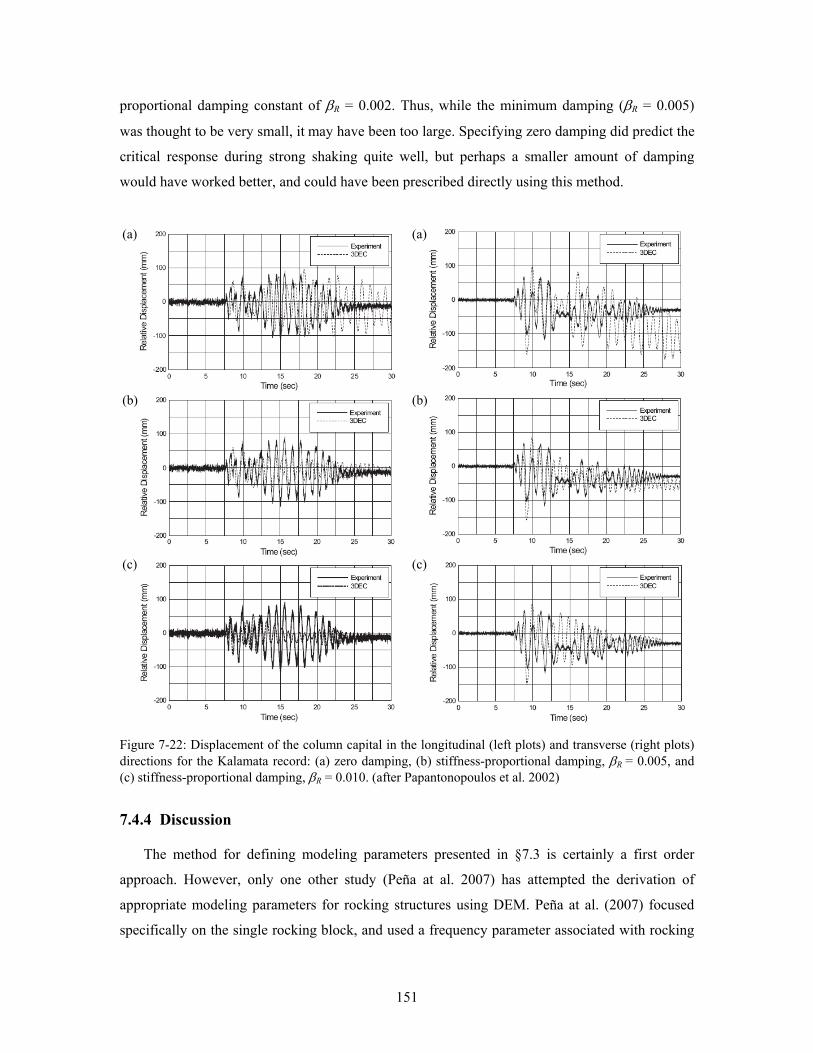
151

proportional damping constant of βR = 0.002. Thus, while the minimum damping (βR = 0.005)

was thought to be very small, it may have been too large. Specifying zero damping did predict the

critical response during strong shaking quite well, but perhaps a smaller amount of damping

would have worked better, and could have been prescribed directly using this method.

Figure 7-22: Displacement of the column capital in the longitudinal (left plots) and transverse (right plots) directions for the Kalamata record: (a) zero damping, (b) stiffness-proportional damping, βR = 0.005, and (c) stiffness-proportional damping, βR = 0.010. (after Papantonopoulos et al. 2002)

7.4.4 Discussion

The method for defining modeling parameters presented in §7.3 is certainly a first order

approach. However, only one other study (Peña at al. 2007) has attempted the derivation of

appropriate modeling parameters for rocking structures using DEM. Peña at al. (2007) focused

specifically on the single rocking block, and used a frequency parameter associated with rocking

(a)

(b)

(c)

(a)

(b)

(c)

152

motion to define the joint stiffness properties. Thus, the joint stiffness was tailored to produce the

appropriate rocking response instead of being specified according to the expected deformation in

the system. The extremely soft joints which result have no physical basis and cause the block to

never lose contact with the ground during the simulated rocking response. The derived DEM

parameters are then adjusted by a fitting procedure to produce the experimentally measured

rotation angle of the block. While this fitting provides extremely accurate results, it approximates

the measured energy dissipation at impact with an equivalent viscous damping over the entire

rocking motion. Thus, this approach is not realistic for assessment of masonry structures in

general.

The presented method fills a critical gap in the process of applying DEM to assess masonry

structures under dynamic loading, by providing a rational basis from which to assign parameters

and begin modeling. Without such a basis, researchers have typically tested a random range of

parameters and determined the sensitivity of results (as in §7.2), but have risked the possibility of

missing the appropriate range of parameters entirely. Furthermore, the method presented in §7.3

has the benefits of being simple and easily applicable, while effectively explaining the results

presented throughout this chapter. However, there are clear limitations:

• The method provides a physical basis for the joint stiffness, but only provides an order of

magnitude estimate of appropriate damping for the system. Thus, informed by the derived

impact frequencies, a sensitivity analysis for a range of frequencies is still necessary.

• The method specifies critical damping to the impact frequency, thus producing plastic

impact. While this seems to be effective for masonry, further validation is necessary. This

is certainly not realistic for materials which behave more elastically during impact.

However, using this method, the fraction of damping during impact for a given material

could be measured and then directly specified at the approximated impact frequency.

• The derivation is based on relatively low frequency ground motions, for which vibration

displacements are unlikely. However, for ground motions with a significant high

frequency component, vibration displacements would likely occur. The effectiveness of

this method for those situations must be investigated.

• When the system consists of multiple blocks of vastly different size, defining modeling

parameters is more involved. The joint stiffness and damping of every joint could be

described individually, but would be quite tedious. Alternatively, one damping level

could be prescribed for the entire model. In this case, deriving damping properties using

the smallest block in the system would produce the largest impact frequencies, the least

153

amount of damping, and thus conservative results. However, sensitivity studies would be

even more important in this case.

In addition to these limitations, it must be stated that it is impossible to predict exact response

of any structures using DEM, especially multiple block systems under complex loadings. This is

evident in the fact that experiments themselves are often not reproducible due to tiny

imperfections in the geometry and minor differences in the ground motion (e.g. Yim et al. 1980,

Mouzakis et al. 2002, Peña et al. 2007). Thus, while these methods effectively improve results,

DEM must be applied with this in mind. Furthermore, this highlights the importance of

understanding structural behavior, and using DEM accordingly. A good example of this is the

approach taken to arch assessment in this dissertation. Using DEM to predict the exact

displacement of every block in the arch during an earthquake is unrealistic. However, first

understanding that the arch is fundamentally vulnerable to impulse loading, allows utilization of

DEM for a much simpler load case. Thus, applying DEM in simpler situations, for example the

dynamic collapse of a buttressed barrel vault under impulse loading (§7.3.4), can provide insight

into specific modes of collapse. Subsequently, behavior under more complex ground motions can

be attempted. Comparison of results can then lead to a determination of what is fundamentally

important in assessing structures.

7.5 Summary

Discrete element modeling is a powerful method with potential for capturing the dynamic

response of masonry structures. The detailed comparisons with analytical modeling, the method

for deriving input parameters, and the sensitivity studies herein allow the following conclusions

to be drawn:

• For the rocking block, DEM results compared well with both the analytical and

experimental rocking block response.

• For the rocking arch, results of numerical modeling are in good agreement with analytical

results, both in terms of behavior and the predicted failure domain.

• Both analytical modeling and numerical modeling provide a means for determining the

minimum coefficient of friction theoretically required to prevent sliding. For the arches

investigated, the coefficient of friction required is below the typical values of masonry

joints, and hence the assumption of no sliding is reasonable.

154

• Specifying a desired damping at the critical frequencies of the system effectively prevents

erroneous numerical prediction of bouncing behavior and vibration displacements.

Accordingly, the proposed method provides an effective basis from which to specify

modeling parameters.

• The sensitivity of numerical modeling results to input parameters is integral to the

confidence in results and to the potential of DEM. Therefore, a sensitivity analysis is

essential. The predicted rocking block response and rocking arch failure domains were

shown to be relatively insensitive to the parameters specified.

155

Part IV

Conclusions

156

Chapter 8

Conclusions

8.1 Summary of Main Findings

The primary objective of this research, as stated in §1.3, is twofold: (1) To increase

fundamental understanding of the dynamic behavior of masonry structures under eathquake

loading, and (2) to develop tested analysis methods that allow appropriate assessment of masonry

structures which might be subjected to earthquake loading. While working towards these

objectives, new and existing analysis methods were created or improved, and applied and tested.

The main findings are as follows:

• Tilting Thrust-Line Analysis: Tilting thrust-line analysis provides a graphical evaluation

of stability under constant horizontal acceleration. The parametric and visual

characteristics are particularly useful for understanding the behavior of vaulted masonry

structures, and exploring the interaction of structural components (e.g. arches, buttresses,

vaults). Stability during earthquakes, approximated by the tilt capacity, was found to be

highly dependent on the spatial relationship of these components. Furthermore, tilting

solutions identified geometries which optimize the interaction of components. The

framework predicted collapse mechanisms which were not initially intuitive and could

not be easily predicted.

157

• Sequentially Linear Analysis: The extension of sequentially linear analysis to include

non-proportional loading allows the self-weight of the structure to be included, enabling

its application to masonry structures under quasi-static seismic loading. This extension

was verified through comparison of SLA results with incrementally iterative non-linear

analysis results. The new framework accurately predicted experimental results involving

brittle fracture of concrete blocks. Additionally, experiments involving horizontal cyclic

loading of a full-scale two-story masonry structure were effectively simulated using SLA

with shell elements. Thus, the method was shown to have potential for predicting damage

to masonry structures during earthquakes.

• Dynamics of Arches: A SDOF analytical model with a reflecting four-hinge mechanism

qualitatively describes the behavior of a rocking arch under horizontal ground motion.

This analytical model was successfully used to predict the collapse of experimentally

tested masonry arches. Results show that the primary impulse within the ground motion

is critical in causing collapse. A single impulse can cause two modes of arch collapse

which parallel the collapse modes of a single rocking block.

• Rocking Structures: The natural rocking period increases with the magnitude of rocking

motion, so constant frequency rocking resonance can not occur. Instead, rocking

resonance is identified for ground motions with constantly increasing periods.

Furthermore, if likely imperfections in the rocking system are included, overturning of a

single rocking block is possible at lower ground accelerations than previously considered.

Although the primary impulse of the ground motions is crucial in causing collapse, it is

possible that multiple distinct impulses could act together to amplify motion. Considering

the uncertain characteristics of possible ground motions and the sensitivity of the rocking

response, a statistical approach is necessary to assess this possibility of multiple impulse

amplification. Results from a statistical analysis showed a wide range in possible

responses for earthquakes of exactly the same frequency content, demonstrating the time

dependence of rocking motion.

• Discrete Element Modeling: Discrete element modeling can effectively predict the

response of rocking structures, but damping must be defined appropriately and the

sensitivity of the results to the assigned damping must be investigated. Mass-proportional

damping is not realistic and should not be used. Stiffness-proportional damping, while

not being physically accurate, should be prescribed to damp unrealistic high frequency

vibrations which occur during numerical modeling. The proposed method for defining

158

stiffness-proportional damping proved a functional approach when simulating

experimental and analytical results. Finally, DEM was found to be useful in predicting

general behavior, but not the exact displacement of an individual block within a large

system. The unknowns of the problem are too many to expect this kind of accuracy.

8.2 Primary Contributions

Based on the main findings above, the two aspects of the primary objective in §1.3 have been

addressed. This dissertation has provided: (1) an increased understanding of the stability and

fundamental behavior of masonry structures under both static and dynamic loading, and (2) new

and improved tools for assessing masonry structures. Specifically, the primary contributions are

as follows:

• Development of tilting thrust-line analysis: This graphical equilibrium tool allows first-

order assessment and a new perspective regarding the stability of vaulted structures under

lateral loading.

• Extension of SLA to non-proportional loading: This extension allows the inclusion of

self-weight in analysis, which is critical for the prediction of damage under simplified

quasi-static seismic loading. This improvement provides a practical tool for assessing and

predicting damage to masonry structures.

• Characterization of the rocking of arches under horizontal ground motion: A new

analytical tool and an experimental program involving small-scale arches describe and

evaluate the rocking behavior of arches for the first time. Additionally, the first seismic

assessment criterion for masonry arches which considers dynamic rocking behavior is

presented.

• Redefinition of the vulnerability of rocking structures to horizontal ground motion: An

energy approach was applied which provides a fresh perspective to an old problem, and

reveals the possibility of rocking resonance. This motivated a new statistical approach

which incorporates past earthquake data and analytical models into a tool for predicting

the probability of rocking collapse during an earthquake of an expected intensity.

• Improved application of discrete element modeling: The evaluation of DEM through

comparison with experimental and analytical results provides confidence in, and a

159

perspective of, modeling capabilities. A method for defining discrete element modeling

parameters is proposed, allowing a more informed application of this tool.

These contributions can lead to more informed assessment of the safety of masonry structures

throughout the world.

8.3 Future Research

The development and application of seismic assessment tools and the experimental

investigations herein contribute towards better assessment of masonry structures in seismic

regions, but also motivate numerous areas of continued research:

• Graphical methods: First, tilting thrust-line analysis could be applied to assess multiple

structures with similar cross-sections, with the goal of pinpointing the least stable. An

ideal resource for such a study would be the database of Bourbonnais churches assembled

by researchers at Columbia University (Murray 2009). Second, this graphical method

could be made more powerful by implementation in a more flexible geometric computing

environment, e.g. Generative Components. This would also allow more adaptability after

constructions have been made, and could facilitate some inclusion of three-dimensional

effects. Finally, the concept of tilting could be implemented in three-dimensions, but this

would require a completely different graphical framework, such as that proposed by

Block and Ochsendorf (2007).

• Strength methods: First, SLA currently employs a uni-axial failure criterion, which

should be improved to a bi-axial failure criterion to better capture failure under non-

proportional loading. Second, the computational solution procedure is currently quite

inefficient and should be improved to account for the fact that only a single element is

updated between each linear analysis. This could significantly shorten run-times. Third,

the algorithm developed for non-proportional loading could be implemented in lattice

modeling frameworks. Finally, with these improvements, SLA could be applied to better

understand and predict damage to shell structures such as vaults and domes.

• Analytical modeling: With a better understanding of rocking behavior and the analytical

models developed herein, optimized methods for structural retrofit could be investigated.

Specifically, the effect of adding damping and stiffness on the rocking response is of

interest, and could explain past destructive interventions to historic masonry structures.

Additionally, the analytical arch model motivates similar simplification of other

160

structures to SDOF systems which could be modeled analytically. New analytical models

could be verified experimentally and numerically through the methods applied in this

dissertation.

• Discrete element modeling: First, further experimental evaluation of discrete element

modeling is necessary, particularly in three-dimensions. Second, the method for defining

damping parameters should be further evaluated and improved. This could be done by

measuring experimentally determining energy dissipation at impact as a material

property, and then prescribing the damping accordingly. Additionally, the effect of

damping parameters on experimentally realized vibration displacements should be

investigated.

In addition to these areas of future research which directly relate to the contributions herein,

one final comment must be made. There is a definite need to identify what information can be

drawn from computer modeling of historic masonry structures, especially under earthquake

loading. The unknowns (e.g. earthquake characteristics, material properties, damage, geometry,

etc.) often do not warrant the extremely complex analyses employed, which perhaps confuse the

evaluation of masonry structures rather than clarify it. The primary challenge is to utilize the tools

which are available, while maintaining a realistic perspective on what can be determined.

161

Part V

Appendices

162

Appendix A

Notation

The following notation is used in this dissertation:

ap = magnitude of a step impulse of ground acceleration

ag = ground acceleration constraint used for optimization

iAω = mean amplitude for spectral frequency ω

Ah = amplitude of harmonic motion

Ap = amplitude of a single sinusoidal ground acceleration impulse

B = block width

cv = coefficient of restitution with respect to the rotational velocity

cE = coefficient of restitution with respect to the total energy

C = damping matrix

E = elastic modulus

ET = total energy in a system

f = frequency [Hz]

fcrit = frequency at which the system is critically damped (ξ = 100%)

fmin = frequency at which Rayleigh damping has a minimum

ft = material tensile strength

+tif = current tensile strength used in Sequentially Linear Analysis

163

F = applied force

G = shear modulus

Gf = material fracture energy

Gred = reduced shear modulus after cracking for Sequentially Linear Analysis

h = crack bandwidth

H = block height

j = integration point identifier

J = mass moment of inertia of a rectangular block about its corner

kj = joint stiffness

ks = spring stiffness

K = stiffness matrix

L_ = angular momentum about point _

mB = mass of a block

M = mass matrix

n- = primary crack normal direction in the plane of the finite element

nA = number of voussoirs in a part-circular arch

p = parameter which modulates the fineness of the saw-tooth constitutive model

px , py = linear momentum in the x- and y- directions

P(t) = intensity function used for earthquake generation

RA = center-line radius of a part-circular arch

s- = secondary crack normal direction in the plane of the finite element

t = time

t- = thickness direction (normal to the mid-surface of the finite element)

tA = thickness of a part-circular arch

td = generated earthquake duration

tp = duration of a step impulse of ground acceleration.

Tn = natural rocking period

Tp = period of a single sinusoidal ground acceleration impulse

gu = horizontal ground acceleration

hu = horizontal acceleration

vu = vertical acceleration

α = ground surface tilt angle

αcr = critical ground surface tilt angle

164

αexp = experimentally measured critical ground surface tilt angle

αR = mass-proportional constant of Rayleigh damping

βA = angle of embrace of a part-circular arch

βR = stiffness-proportional constant of Rayleigh damping

βsh = shear retention factor

γ = minimum horizontal acceleration which causes collapse [g]

γ80 = theoretical γ using 80% of the arch thickness

γexp = value of γ calculated from the measured critical ground surface tilt angle

γns , γst , γtn = shear strain in the subscript directions

δ = displacement

ε = strain

εnn , εss , εtt = normal strain in the subscript directions

εu = ultimate normal strain for the linear softening constitutive model

θ = rotation angle of the rocking arch or the rocking block

θcr = critical rotation angle of a rocking block

θs = static (at-rest) rotational displacement

θ = rotational velocity

∗afterθ = rotational velocity immediately after impact

beforeθ = rotational velocity immediately before impact

′θ = derivative of the rocking angle with respect to the dimensionless time τ

′′θ = derivative of θ ′ with respect to the dimensionless time τ

λ = load multiplier for Sequentially Linear Analysis

λ1, λ2 = load multipliers for each integration point under non-proportional loading

λcrit = critical load multiplier for Sequentially Linear Analysis

cjλ = load multiplier for integration point j which causes a compressive stress ,Bϕσ

tjλ = load multiplier for integration point j which causes a tensile stress ,Bϕσ

μ = coefficient of friction

ν = Poisson’s ratio

ξ = fraction of critical damping

ξmin = minimum fraction of critical damping at fmin for Rayleigh damping

ρ = material density

165

σ = stress

σ 1, σ 2 = principal stresses

σA , σ--,A = stress due to application of load A

σB , σ--,B = stress due to application of load B

σt = maximum principal tensile stress at each integration point

,Bϕσ = stress in the principal stress direction due to application of load B

τ = dimensionless time

φ = rotation angle of the rocking arch

φcr = critical rotation angle of a rocking arch

iωφ = phase angle for spectral frequency ω

ϕ 1, ϕ 2 = principal stress directions

ω = frequency [radians]

Δω = frequency step used for earthquake generation

ωc = natural frequency associated with corner impact

ωcrit = frequency at which the system is critically damped (ξ = 100%) [radians]

ωe = natural frequency associated with edge impact

ωr = natural frequency associated with rotational impact

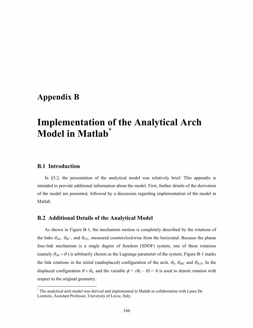
166

Appendix B

Implementation of the Analytical Arch Model in Matlab*

B.1 Introduction

In §5.2, the presentation of the analytical model was relatively brief. This appendix is

intended to provide additional information about the model. First, further details of the derivation

of the model are presented, followed by a discussion regarding implementation of the model in

Matlab.

B.2 Additional Details of the Analytical Model

As shown in Figure B-1, the mechanism motion is completely described by the rotations of

the links θAB , θBC , and θCD , measured counterclockwise from the horizontal. Because the planar

four-link mechanism is a single degree of freedom (SDOF) system, one of these rotations

(namely θAB = θ ) is arbitrarily chosen as the Lagrange parameter of the system. Figure B-1 marks

the link rotations in the initial (undisplaced) configuration of the arch, θ0, θ0BC and θ0CD. In the

displaced configuration θ < θ0, and the variable φ = (θ0 – θ) > 0 is used to denote rotation with

respect to the original geometry. * The analytical arch model was derived and implemented in Matlab in collaboration with Laura De Lorenzis, Assistant Professor, University of Lecce, Italy.

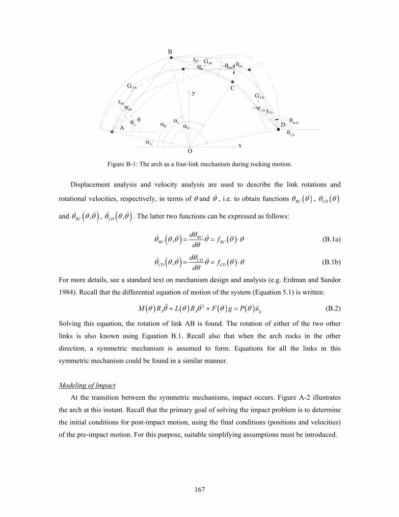
167

A

B

C

D

GAB

GBC

GCDrAB

rBC

rCDψAB

ψBC

−ψCD

αA

αBαC

αD

y

x

θ0θ0CD

−θ0BC

O

θ

θCD

θBC

Figure B-1: The arch as a four-link mechanism during rocking motion.

Displacement analysis and velocity analysis are used to describe the link rotations and

rotational velocities, respectively, in terms of θ and θ , i.e. to obtain functions ( )BCθ θ , ( )CDθ θ

and ( ),BCθ θ θ , ( ),CDθ θ θ . The latter two functions can be expressed as follows:

( ) ( ), = = ⋅BCBC BC

d fdθ

θ θ θ θ θ θθ

(B.1a)

( ) ( ), = = ⋅CDCD CD

d fdθ

θ θ θ θ θ θθ

(B.1b)

For more details, see a standard text on mechanism design and analysis (e.g. Erdman and Sandor

1984). Recall that the differential equation of motion of the system (Equation 5.1) is written:

( ) ( ) ( ) ( )2+ + =A A gM R L R F g P uθ θ θ θ θ θ (B.2)

Solving this equation, the rotation of link AB is found. The rotation of either of the two other

links is also known using Equation B.1. Recall also that when the arch rocks in the other

direction, a symmetric mechanism is assumed to form. Equations for all the links in this

symmetric mechanism could be found in a similar manner.

Modeling of Impact

At the transition between the symmetric mechanisms, impact occurs. Figure A-2 illustrates

the arch at this instant. Recall that the primary goal of solving the impact problem is to determine

the initial conditions for post-impact motion, using the final conditions (positions and velocities)

of the pre-impact motion. For this purpose, suitable simplifying assumptions must be introduced.

168

A

B

C

D

αA

αBαC

αD

y

xO

A

BC

D

FA FD

Figure B-2: The arch at the instant of the impact.

It is assumed that the position of the system does not vary during impact, while its velocities

are subjected to an instantaneous variation due to the action of impulsive forces. Impact occurs at

the hinge sections, where contact generally involves a finite area which is a priori unknown. In

analogy with Housner’s treatment of impact of the single rocking block (Housner 1963), the

impulsive force at each hinge section is assumed to be located on the opposite side of the hinge

across the arch thickness, i.e. at points A , B , C and D (Figure B-2).

At the location of the internal hinges B and C, the impact generates internal impulsive forces

which balance each other. At the locations of the extreme hinges A and D, external impulsive

forces AF and DF arise. The problem can be formulated considering five unknowns, namely: the

x- and y- components of AF and DF ( AxF , AyF , DxF , DyF ), plus the rotational velocity of link A*B*

(see Figure 5-1) immediately after impact, ∗afterθ . The five equations used to determine these

unknowns are:

The equation of linear momentum in the x-direction for the whole arch:

,∗ ∗Δ − Δ − = −x after x beforeAx DxF t F t k pθ (B.3a)

The equation of linear momentum in the y-direction for the whole arch:

,∗ ∗Δ + Δ − = −y after y beforeAy DyF t F t k pθ (B.3b)

The equation of angular momentum about O for the whole arch:

,0 0 0 0∗ ∗− Δ ⋅ + Δ ⋅ + Δ ⋅ + Δ ⋅ − = −O after O iAx A Ay A Dx D Dy DF t y F t x F t y F t x k Lθ (B.3c)

169

The equation of angular momentum about B for the portion of the arch to the left of B :

( ) ( )0 0 0 0 ,∗ ∗Δ ⋅ − − Δ ⋅ − − = −afterBAx B A Ay B A B beforeF t y y F t x x k Lθ (B.3d)

The equation of angular momentum about C for the portion of the arch to the right of C :

( ) ( )0 0 0 0 ,∗ ∗− Δ ⋅ − + Δ ⋅ − − = −afterCDx C D Dy D C C beforeF t y y F t x x k Lθ (B.3e)

where Δt is the duration of the impact, the ∗−k terms are known geometric coefficients, the

_ ,beforep and _ ,beforeL terms are known quantities of linear and angular momentum immediately

before impact, and the 0 _x and 0 _y terms are known x- and y- coordinates of points in the initial

(undisplaced) configuration of the arch. In writing the equations, self-weights are neglected

because they are small compared to impulsive forces, as is normally assumed for impact

problems. By solving the system of equations, the angular velocity immediately after impact

( ∗afterθ ) is computed.

B.3 Implementation in Matlab

The differential equations of motion (Equations 5.1 and 5.2) were solved using the ode45

algorithm in Matlab. This algorithm is based on an explicit Runge-Kutta (4,5) formula (Dormand

and Prince 1980). It is a one-step solver, and therefore needs only the results from the previous

time step to solve the equation of motion in the current time step.

The entire Matlab code is not included herein, but a graphical user interface (GUI) was built

to provide a tool which can be used to predict the response of arches to any ground motion. This

allowed the model to be run repeatedly to obtain the results included in this dissertation.

Figure B-3 is a screen image of the GUI. The top section of the GUI allows the input of the

desired arch geometry. Using this information, the constant horizontal acceleration which would

cause collapse (γ) is determined (in this case 0.33g), and the hinge locations of the corresponding

collapse mechanism are plotted. This static problem is solved numerically using Matlab, but gives

an equivalent result to the graphical method of tilting thrust-line analysis presented in §3.3.

The middle section of the GUI allows the input of the desired horizontal ground acceleration.

The ground acceleration can be input as either a single impulse or an acceleration time history.

For a single impulse, the impulse characteristics are input directly into the GUI, and solving

commences when the appropriate button is clicked. For an acceleration impulse, a data file with

an acceleration time history is placed in the same directory as the GUI, and is read as input. In

Figure B-3, a time history was applied and the resulting rocking angle is plotted. In this case, the

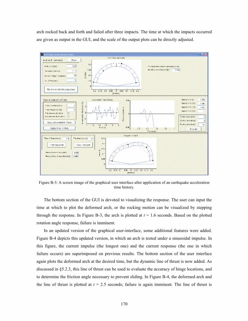
170

arch rocked back and forth and failed after three impacts. The time at which the impacts occurred

are given as output in the GUI, and the scale of the output plots can be directly adjusted.

Figure B-3: A screen image of the graphical user interface after application of an earthquake acceleration time history.

The bottom section of the GUI is devoted to visualizing the response. The user can input the

time at which to plot the deformed arch, or the rocking motion can be visualized by stepping

through the response. In Figure B-3, the arch is plotted at t = 1.6 seconds. Based on the plotted

rotation angle response, failure is imminent.

In an updated version of the graphical user-interface, some additional features were added.

Figure B-4 depicts this updated version, in which an arch is tested under a sinusoidal impulse. In

this figure, the current impulse (the longest one) and the current response (the one in which

failure occurs) are superimposed on previous results. The bottom section of the user interface

again plots the deformed arch at the desired time, but the dynamic line of thrust is now added. As

discussed in §5.2.3, this line of thrust can be used to evaluate the accuracy of hinge locations, and

to determine the friction angle necessary to prevent sliding. In Figure B-4, the deformed arch and

the line of thrust is plotted at t = 2.5 seconds; failure is again imminent. The line of thrust is

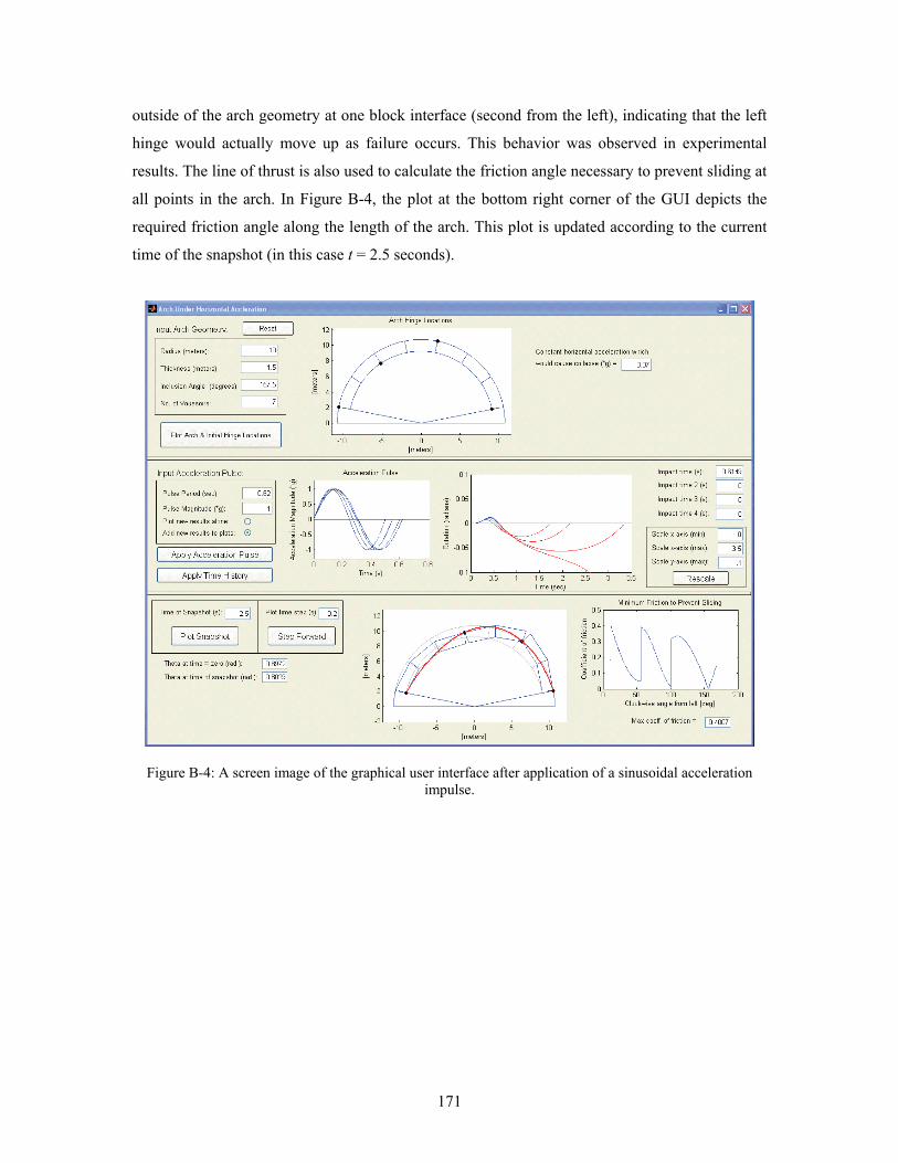
171

outside of the arch geometry at one block interface (second from the left), indicating that the left

hinge would actually move up as failure occurs. This behavior was observed in experimental

results. The line of thrust is also used to calculate the friction angle necessary to prevent sliding at

all points in the arch. In Figure B-4, the plot at the bottom right corner of the GUI depicts the

required friction angle along the length of the arch. This plot is updated according to the current

time of the snapshot (in this case t = 2.5 seconds).

Figure B-4: A screen image of the graphical user interface after application of a sinusoidal acceleration impulse.

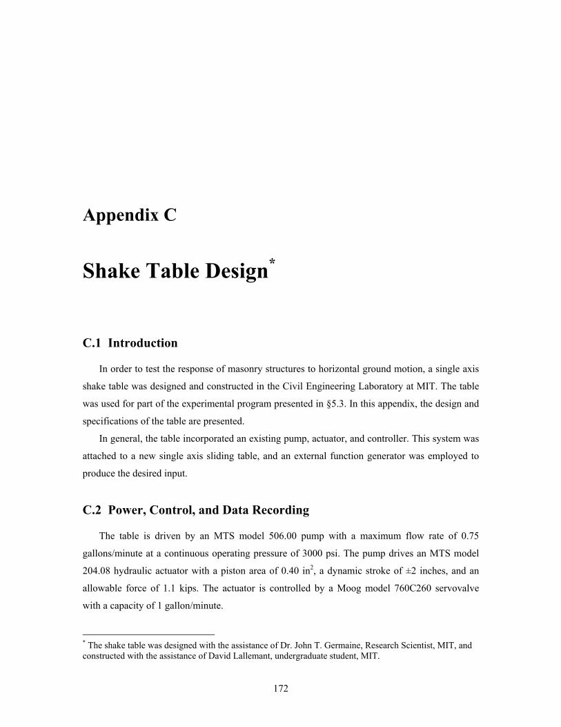
172

Appendix C

Shake Table Design*

C.1 Introduction

In order to test the response of masonry structures to horizontal ground motion, a single axis

shake table was designed and constructed in the Civil Engineering Laboratory at MIT. The table

was used for part of the experimental program presented in §5.3. In this appendix, the design and

specifications of the table are presented.

In general, the table incorporated an existing pump, actuator, and controller. This system was

attached to a new single axis sliding table, and an external function generator was employed to

produce the desired input.

C.2 Power, Control, and Data Recording

The table is driven by an MTS model 506.00 pump with a maximum flow rate of 0.75

gallons/minute at a continuous operating pressure of 3000 psi. The pump drives an MTS model

204.08 hydraulic actuator with a piston area of 0.40 in2, a dynamic stroke of ±2 inches, and an

allowable force of 1.1 kips. The actuator is controlled by a Moog model 760C260 servovalve

with a capacity of 1 gallon/minute.

* The shake table was designed with the assistance of Dr. John T. Germaine, Research Scientist, MIT, and constructed with the assistance of David Lallemant, undergraduate student, MIT.

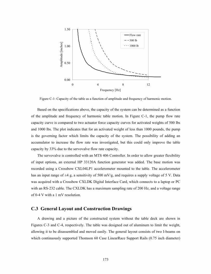
173

0.00

0.50

1.00

1.50

0 4 8 12

Frequency [Hz]

Am

plitu

de [i

nche

s]

Flow rate

500 lb

1000 lb

Figure C-1: Capacity of the table as a function of amplitude and frequency of harmonic motion.

Based on the specifications above, the capacity of the system can be determined as a function

of the amplitude and frequency of harmonic table motion. In Figure C-1, the pump flow rate

capacity curve is compared to two actuator force capacity curves for activated weights of 500 lbs

and 1000 lbs. The plot indicates that for an activated weight of less than 1000 pounds, the pump

is the governing factor which limits the capacity of the system. The possibility of adding an

accumulator to increase the flow rate was investigated, but this could only improve the table

capacity by 33% due to the servovalve flow rate capacity.

The servovalve is controlled with an MTS 406 Controller. In order to allow greater flexibility

of input options, an external HP 33120A function generator was added. The base motion was

recorded using a Crossbow CXL04LP1 accelerometer mounted to the table. The accelerometer

has an input range of ±4 g, a sensitivity of 500 mV/g, and requires a supply voltage of 5 V. Data

was acquired with a Crossbow CXLDK Digital Interface Card, which connects to a laptop or PC

with an RS-232 cable. The CXLDK has a maximum sampling rate of 200 Hz, and a voltage range

of 0-4 V with a 1 mV resolution.

C.3 General Layout and Construction Drawings

A drawing and a picture of the constructed system without the table deck are shown in

Figures C-3 and C-4, respectively. The table was designed out of aluminum to limit the weight,

allowing it to be disassembled and moved easily. The general layout consists of two I-beams on

which continuously supported Thomson 60 Case LinearRace Support Rails (0.75 inch diameter)

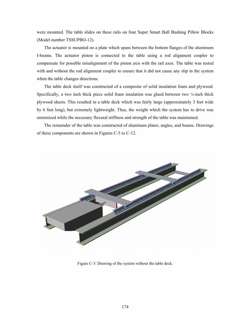
174

were mounted. The table slides on these rails on four Super Smart Ball Bushing Pillow Blocks

(Model number TSSUPBO-12).

The actuator is mounted on a plate which spans between the bottom flanges of the aluminum

I-beams. The actuator piston is connected to the table using a rod alignment coupler to

compensate for possible misalignment of the piston axis with the rail axes. The table was tested

with and without the rod alignment coupler to ensure that it did not cause any slip in the system

when the table changes directions.

The table deck itself was constructed of a composite of solid insulation foam and plywood.

Specifically, a two inch thick piece solid foam insulation was glued between two ¼-inch thick

plywood sheets. This resulted in a table deck which was fairly large (approximately 3 feet wide

by 6 feet long), but extremely lightweight. Thus, the weight which the system has to drive was

minimized while the necessary flexural stiffness and strength of the table was maintained.

The remainder of the table was constructed of aluminum plates, angles, and beams. Drawings

of these components are shown in Figures C-5 to C-12.

Figure C-3: Drawing of the system without the table deck.

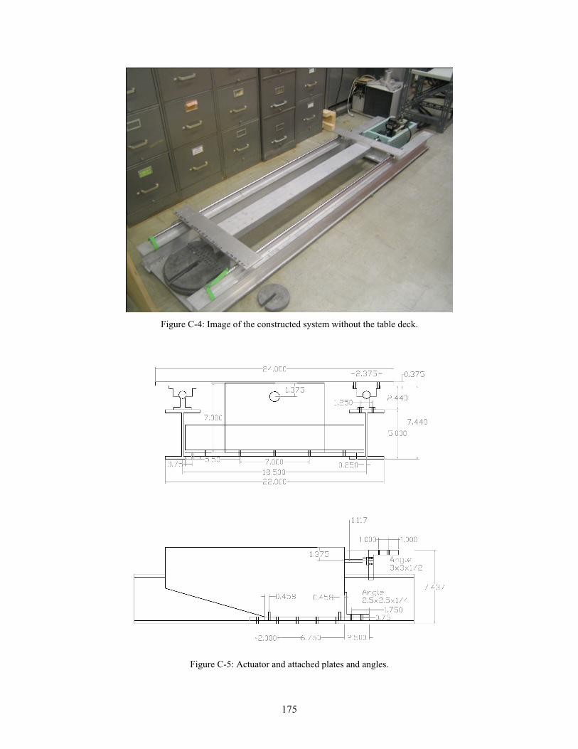
175

Figure C-4: Image of the constructed system without the table deck.

Figure C-5: Actuator and attached plates and angles.

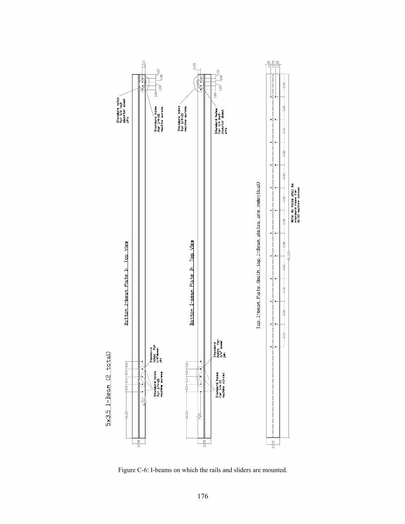
176

Figure C-6: I-beams on which the rails and sliders are mounted.

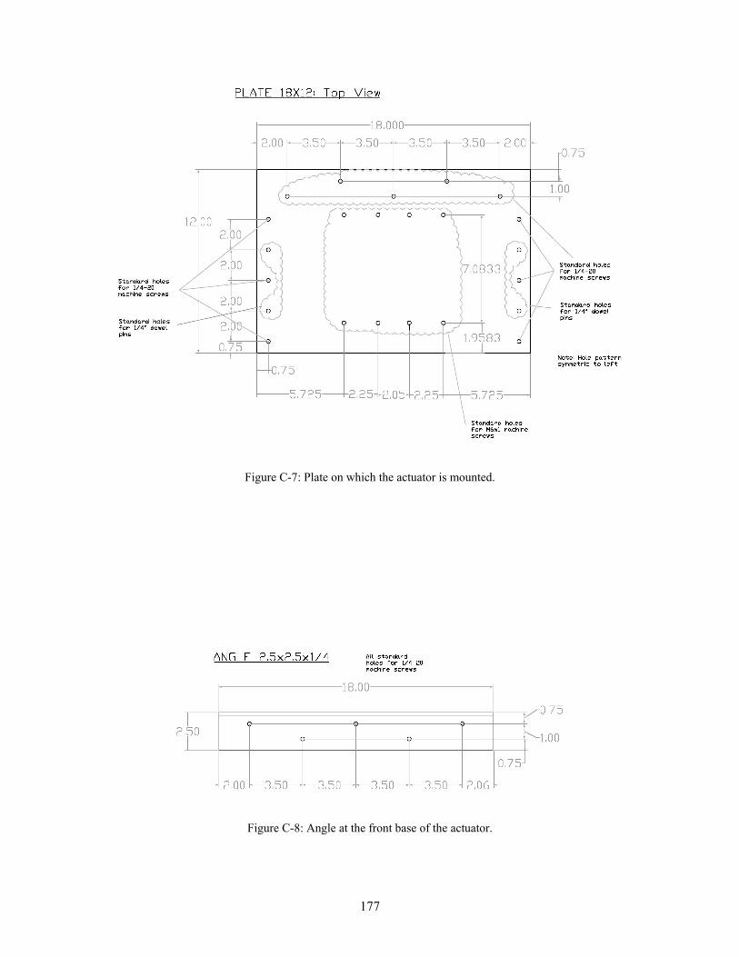
177

Figure C-7: Plate on which the actuator is mounted.

Figure C-8: Angle at the front base of the actuator.

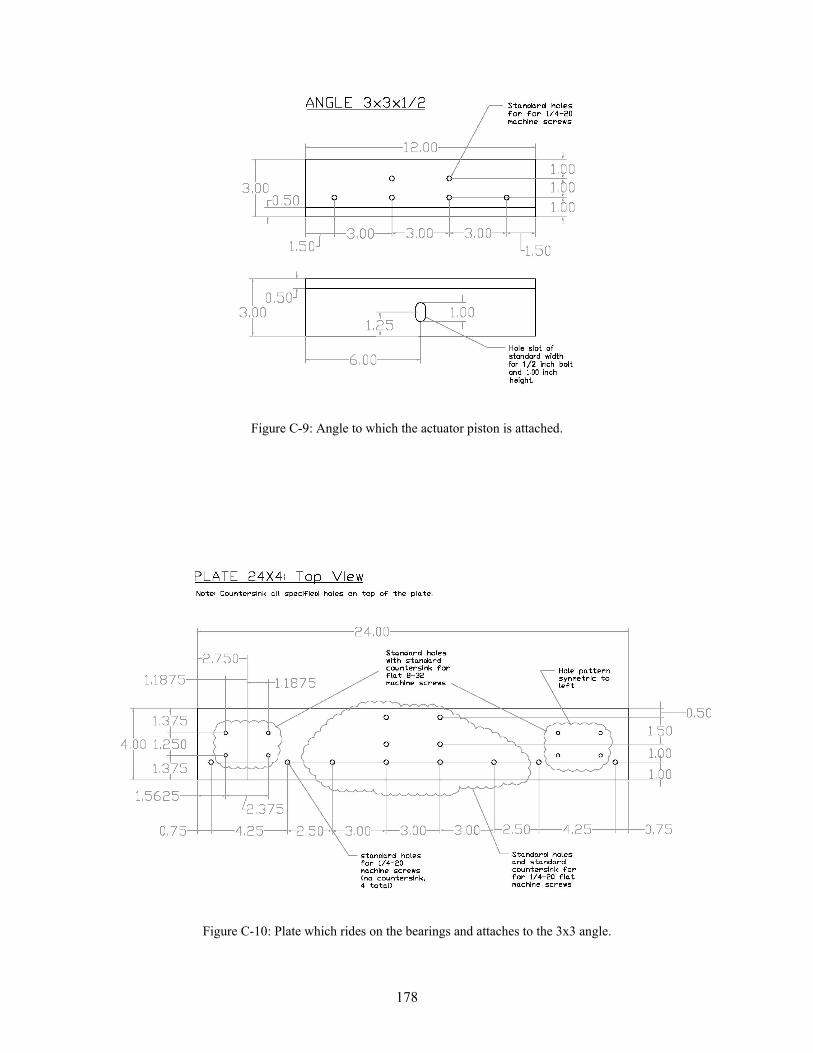
178

Figure C-9: Angle to which the actuator piston is attached.

Figure C-10: Plate which rides on the bearings and attaches to the 3x3 angle.

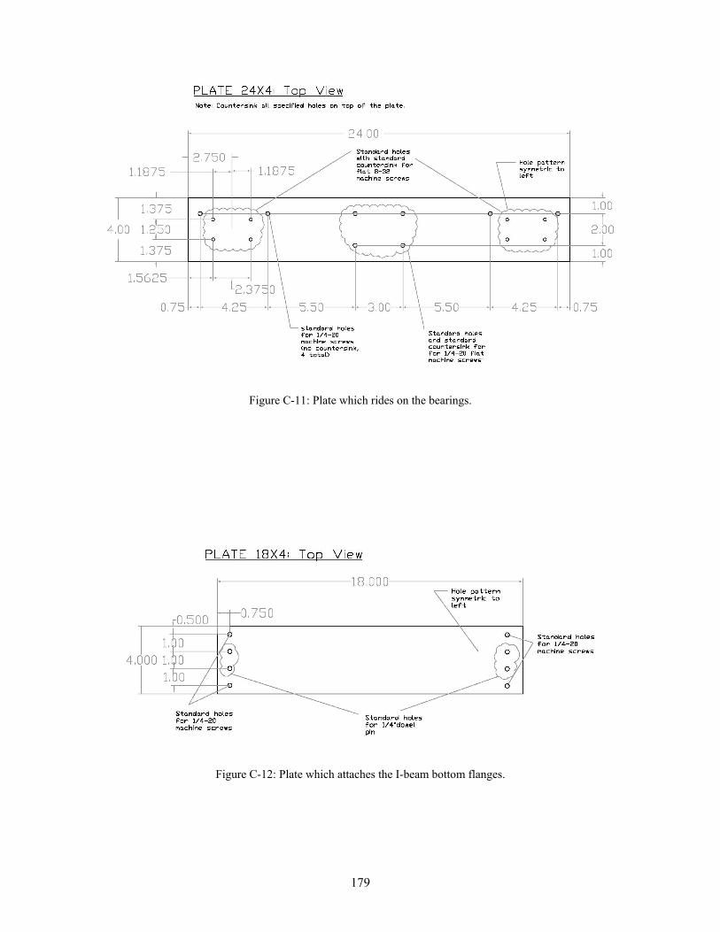
179

Figure C-11: Plate which rides on the bearings.

Figure C-12: Plate which attaches the I-beam bottom flanges.

181

Bibliography

Allen, E. and Zalewski, W. (2009). Form and forces: Designing efficient, expressive structures. New York: John Wiley and Sons.

American Society of Civil Engineers (2000). Prestandard and commentary for the seismic rehabilitation of buildings, FEMA-356.

Appleton, J. (1999). Earthquake response of arches. Fourth-year undergraduate project, University of Cambridge. Cambridge, UK.

Augusti, G. and Sinopoli, A. (1992). Modeling the dynamics of large block structures, Meccanica, 17, 195-211.

Azevedo, J., Sincraian, G. and Lemos, J.V. (2000). Seismic behavior of blocky masonry structures, Earthquake Spectra, 16(2), 337-365.

Bathe, K.J. (2006). Finite element procedures. New Jersey: Prentice Hall.

Block, P. (2005). Equilibrium systems: Studies in masonry structure. S.M. Thesis, Massachusetts Institute of Technology. Cambridge, Massachusetts.

Block, P. and Ochsendorf, J. (2007). Thrust network analysis: a new methodology for three-dimensional equilibrium, Journal of the International Association for Shell and Spatial Structures, 48(3), 167-173.

Bohlen, C. (1997, October 25). Assisi holds its breath and rebuilds treasures, The New York Times, p. A5.

Bolander, J.A. and Saito S. (1998). Fracture analyses using spring networks with random geometry, Engineering Fracture Mechanics, 61, 569-591.

Boothby, T.E. (2001). Analysis of masonry arches and vaults, Progress in Structural Engineering and Materials, 3, 246-256.

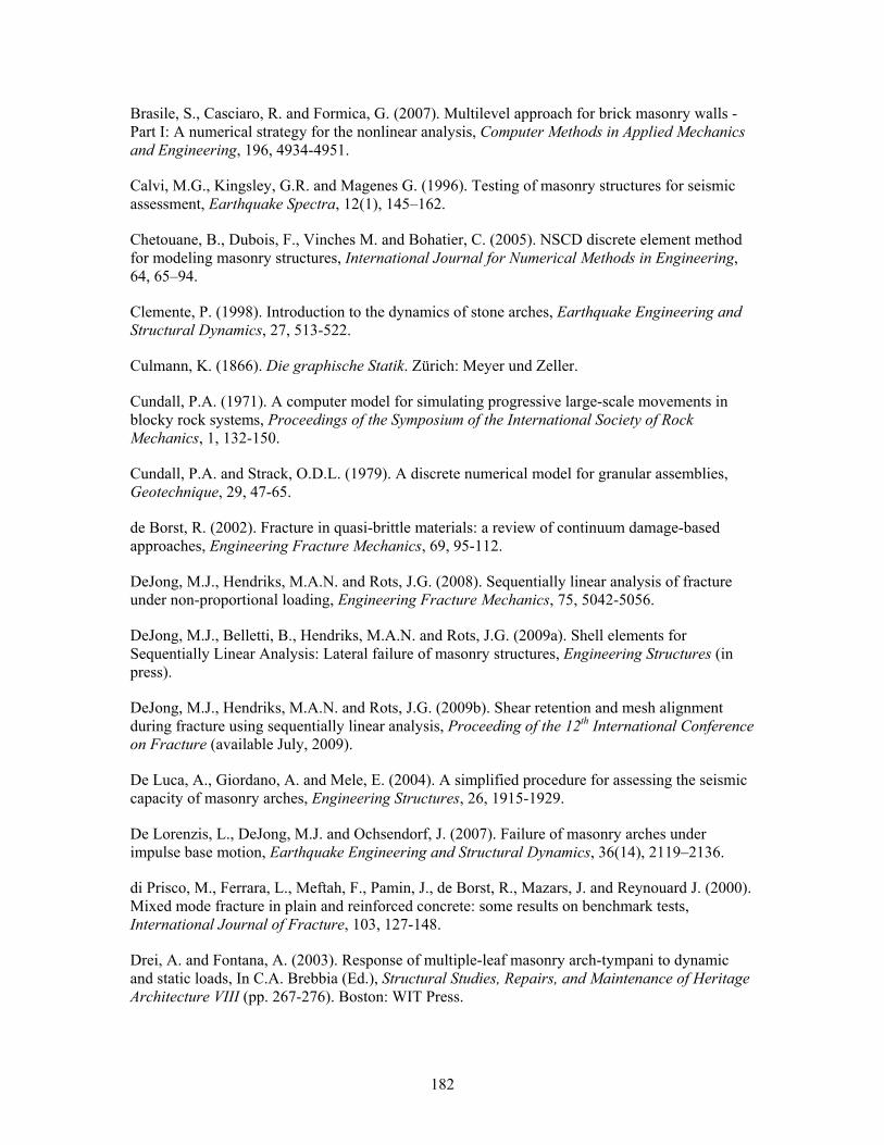
182

Brasile, S., Casciaro, R. and Formica, G. (2007). Multilevel approach for brick masonry walls - Part I: A numerical strategy for the nonlinear analysis, Computer Methods in Applied Mechanics and Engineering, 196, 4934-4951.

Calvi, M.G., Kingsley, G.R. and Magenes G. (1996). Testing of masonry structures for seismic assessment, Earthquake Spectra, 12(1), 145–162.

Chetouane, B., Dubois, F., Vinches M. and Bohatier, C. (2005). NSCD discrete element method for modeling masonry structures, International Journal for Numerical Methods in Engineering, 64, 65–94.

Clemente, P. (1998). Introduction to the dynamics of stone arches, Earthquake Engineering and Structural Dynamics, 27, 513-522.

Culmann, K. (1866). Die graphische Statik. Zürich: Meyer und Zeller.

Cundall, P.A. (1971). A computer model for simulating progressive large-scale movements in blocky rock systems, Proceedings of the Symposium of the International Society of Rock Mechanics, 1, 132-150.

Cundall, P.A. and Strack, O.D.L. (1979). A discrete numerical model for granular assemblies, Geotechnique, 29, 47-65.

de Borst, R. (2002). Fracture in quasi-brittle materials: a review of continuum damage-based approaches, Engineering Fracture Mechanics, 69, 95-112.

DeJong, M.J., Hendriks, M.A.N. and Rots, J.G. (2008). Sequentially linear analysis of fracture under non-proportional loading, Engineering Fracture Mechanics, 75, 5042-5056.

DeJong, M.J., Belletti, B., Hendriks, M.A.N. and Rots, J.G. (2009a). Shell elements for Sequentially Linear Analysis: Lateral failure of masonry structures, Engineering Structures (in press).

DeJong, M.J., Hendriks, M.A.N. and Rots, J.G. (2009b). Shear retention and mesh alignment during fracture using sequentially linear analysis, Proceeding of the 12th International Conference on Fracture (available July, 2009).

De Luca, A., Giordano, A. and Mele, E. (2004). A simplified procedure for assessing the seismic capacity of masonry arches, Engineering Structures, 26, 1915-1929.

De Lorenzis, L., DeJong, M.J. and Ochsendorf, J. (2007). Failure of masonry arches under impulse base motion, Earthquake Engineering and Structural Dynamics, 36(14), 2119–2136.

di Prisco, M., Ferrara, L., Meftah, F., Pamin, J., de Borst, R., Mazars, J. and Reynouard J. (2000). Mixed mode fracture in plain and reinforced concrete: some results on benchmark tests, International Journal of Fracture, 103, 127-148.

Drei, A. and Fontana, A. (2003). Response of multiple-leaf masonry arch-tympani to dynamic and static loads, In C.A. Brebbia (Ed.), Structural Studies, Repairs, and Maintenance of Heritage Architecture VIII (pp. 267-276). Boston: WIT Press.

183

Dormand, J.R. and Prince, P.J. (1980). A family of embedded Runge-Kutta formulae, Journal of Computational and Applied Mathematics, 6, 19-26.

EERI (2005). Learning from Earthquakes: First Report on the Kashmir Earthquake of October 8, 2005, EERI Special Earthquake Report – December 2005. Retrieved March 13, 2009, from EERI Online: [http://www.eeri.org/lfe/clearinghouse/kashmir/observ1.php].

Erdman, A. and Sandor, G. (1984). Mechanism Design: Analysis and Synthesis. New Jersey: Prentice-Hall.

Fallahi, A. (2007). Lessons learned from the housing reconstruction following the Bam Earthquake in Iran, The Australian Journal of Emergency Management, 22(1), 26-35.

Feenstra, P.H., Rots, J.G., Arnesen, A., Teigen, J.G. and Høiseth, K.V. (1998). A 3D constitutive model for concrete based on a co-rotational concept. In R. de Borst et al. (Eds.), EURO-C 1998: Computational Modelling of Concrete Structures (pp. 12-22). Rotterdam: Balkema.

Gambarotta, G. and Lagomarsino, S. (1997a). Damage models for the seismic response of brick masonry shear walls - Part I: The mortar joint model and its applications, Earthquake Engineering and Structural Dynamics, 26, 423-439.

Gambarotta, G. and Lagomarsino, S. (1997b). Damage models for the seismic response of brick masonry shear walls - Part II: The continuum model and its applications, Earthquake Engineering and Structural Dynamics, 26, 441-462.

Gasparini, D.A. and Vanmarcke, E.H. (1976). Simulated earthquake motions compatible with prescribed response spectra. MIT Department of Civil Engineering Research Report R76-4. Cambridge, Massachusetts.

Gaß, S. (1990). IL 25: Experiments. University of Lightweight Structures, Germany: Institute for Lightweight Structures.

Harris, H.G. and Sabnis, G.M. (1999). Structural modeling and experimental techniques (2nd edition). Boca Raton, Florida: CRC Press, Inc.

Herrmann, H.J., Hansen, A. and Roux, S. (1989). Fracture of disordered, elastic lattices in two dimensions, Physical Review B, 39(1), 637-648.

Heyman, J. (1966). The stone skeleton, International Journal of Solids and Structures, 2, 249-279.

Heyman, J. (1995). The Stone Skeleton: Structural engineering of masonry architecture. Cambridge: Cambridge University Press.

Heyman, J. (1998). Structural Analysis: A Historical Approach. Cambridge: Cambridge University Press.

Hogan, S.J. (1990). The many steady state responses of a rigid block under harmonic forcing, Earthquake Engineering and Structural Dynamics, 19, 1057–71.

Hooke, R. (1675). A description of helioscopes, and some other instruments. London.

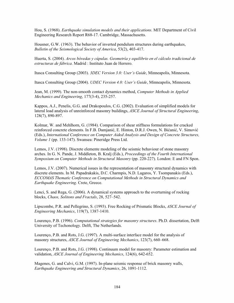
184

Hou, S. (1968). Earthquake simulation models and their applications. MIT Department of Civil Engineering Research Report R68-17. Cambridge, Massachusetts.

Housner, G.W. (1963). The behavior of inverted pendulum structures during earthquakes, Bulletin of the Seismological Society of America, 53(2), 403-417.

Huerta, S. (2004). Arcos bóvedas y cúpulas. Geometría y equilibrio en el cálculo tradicional de estructuras de fábrica. Madrid : Instituto Juan de Herrero.

Itasca Consulting Group (2003). 3DEC Version 3.0: User’s Guide, Minneapolis, Minnesota.

Itasca Consulting Group (2004). UDEC Version 4.0: User’s Guide, Minneapolis, Minnesota.

Jean, M. (1999). The non-smooth contact dynamics method, Computer Methods in Applied Mechanics and Engineering, 177(3-4), 235-257.

Kappos, A.J., Penelis, G.G. and Drakopoulos, C.G. (2002). Evaluation of simplified models for lateral load analysis of unreinforced masonry buildings, ASCE Journal of Structural Engineering, 128(7), 890-897.

Kolmar, W. and Mehlhorn, G. (1984). Comparison of shear stiffness formulations for cracked reinforced concrete elements. In F.B. Damjanić, E. Hinton, D.R.J. Owen, N. Bićanić, V. Simović (Eds.), International Conference on Computer Aided Analysis and Design of Concrete Structures, Volume 1 (pp. 133-147). Swansea: Pineridge Press Ltd.

Lemos, J.V. (1998). Discrete elemente modeling of the seismic behaviour of stone masonry arches. In G. N. Pande, J. Middleton, B. Kralj (Eds.), Proceedings of the Fourth International Symposium on Computer Methods in Structural Masonry (pp. 220-227). London: E and FN Spon.

Lemos, J.V. (2007). Numerical issues in the representation of masonry structural dynamics with discrete elements. In M. Papadrakakis, D.C. Charmpis, N.D. Lagaros, Y. Tsompanakis (Eds.), ECCOMAS Thematic Conference on Computational Methods in Structural Dynamics and Earthquake Engineering. Crete, Greece.

Lenci, S. and Rega, G. (2006). A dynamical systems approach to the overturning of rocking blocks, Chaos, Solitons and Fractals, 28, 527–542.

Lipscombe, P.R. and Pellegrino, S. (1993). Free Rocking of Prismatic Blocks, ASCE Journal of Engineering Mechanics, 119(7), 1387-1410.

Lourenço, P.B. (1996). Computational strategies for masonry structures. Ph.D. dissertation, Delft University of Techonology. Delft, The Netherlands.

Lourenço, P.B. and Rots, J.G. (1997). A multi-surface interface model for the analysis of masonry structures, ASCE Journal of Engineering Mechanics, 123(7), 660–668.

Lourenço, P.B. and Rots, J.G. (1998). Continuum model for masonry: Parameter estimation and validation, ASCE Journal of Engineering Mechanics, 124(6), 642-652.

Magenes, G. and Calvi, G.M. (1997). In-plane seismic response of brick masonry walls, Earthquake Engineering and Structural Dynamics, 26, 1091-1112.

185

Magenes, G. and Della Fontana, A. (1998). Simplified non-linear seismic analysis of masonry buildings. In H.W.H. West (Ed.), Proceedings of the British Masonry Society No.8 (pp. 190-195).

Makris, N. and Konstantinidis, D. (2003). The rocking spectrum and the limitation of practical design methodologies, Earthquake Engineering and Structural Dynamics, 32, 265-289.

Mallardo, V., Malvezzi, R., Milani, E., and Milani, G. (2008). Seismic vulnerability of historical masonry buildings: A case study in Ferrara, Engineering Structures, 30, 2223-2241.

masonry. (2009). In Encyclopædia Britannica. Retrieved March 13, 2009, from Encyclopædia Britannica Online: http://www.britannica.com/EBchecked/topic/368060/masonry.

Matlab (2002). High-performance Language Software for Technical Computation. Natick, MA: The MathWorks, Inc.

Meyer, P., Ochsendorf, J., Germaine, J. and Kausel, E. (2007). The impact of high-frequency/low energy seismic waves on unreinforced masonry, Earthquake Spectra, 23(1), 77–94.

Milani, E., Milani, G. and Tralli, A. (2008). Limit analysis of masonry vaults by means of curved shell finite elements and homogenization, International Journal of Solids and Structures, 45, 5258-5288.

Milani, G., Lourenço, P.B. and Tralli, A. (2006a). Homogenised limit analysis of masonry walls, Part I: Failure surfaces, Computers and Structures, 84, 166-180.

Milani, G., Lourenço, P.B. and Tralli, A. (2006b). Homogenised limit analysis of masonry walls, Part II: Structural examples, Computers and Structures, 84, 181-195.

Milani, G., Lourenço, P.B. and Tralli, A. (2007). 3D homogenized limit analysis of masonry buildings under horizontal loads, Engineering Structures, 29, 3134-3148.

Moon, F.L., Yi, T., Leon, R.T. and Kahn, L.F. (2006). Recommendations for the seismic evaluation and retrofit of low-rise URM structures, ASCE Journal of Structural Engineering, 132(5), 663-672.

Moreau, J.J. (1985). Standard inelastic shocks and the dynamics of unilateral constraints. In G. Del Piero, F. Maceri (Eds.), Unilateral Problems in Structural Analysis, CISM Courses and Lectures No. 288 (pp. 173-221). Wien, New York: Springer-Verlag.

Moreau, J.J. (1988). Unilateral contact and dry friction in finite freedom dynamics. In J.J. Moreau, P.D. Panagiotopoulos (Eds.), Nonsmooth Mechanics and Applications, CISM Courses and Lectures No. 302 (pp. 1-82). Wien, New York: Springer-Verlag.

Mouzakis, H., Psycharis, I.N., Papastamatiou, D.Y., Carydis, P.G., Papantonopoulos, C. and Zambas C. (2002). Experimental investigation of the earthquake response of a model of a marble classical column, Earthquake Engineering and Structural Dynamics, 31, 1681-1698.

Murray, S. (2009). Romanesque Churches of the Bourbonnais [http://www.learn.columbia.edu/bourbonnais/].

186

Nikolinakou, M.A., Tallon, A.J. and Ochsendorf, J.A. (2005). Structure and form of early Gothic flying buttresses, Revue Européenne de Génie Civil, 9(9-10), 1191-1217.

Nooru-Mohamed, M.B. (1992). Mixed mode fracture of concrete: an experimental approach. Ph.D. Dissertation, Delft University of Technology. Delft, The Netherlands.

Nooru-Mohamed, M.B., Schlangen, E. and van Mier, J.G.M. (1993). Experimental and numerical study on the behavior of concrete subjected to biaxial tension and shear, Advanced Cement Based Materials, 1, 22-37.

Ochsendorf, J.A. (2002). Collapse of Masonry Structures, Ph.D. Dissertation, University of Cambridge. Cambridge, UK.

Ochsendorf J.A. and De Lorenzis, L. (2008). Failure of rectangular masonry buttresses under concentrated loading, Proceedings of the Institution of Civil Engineers - Structures and Buildings, 161(5), 265-275.

Oppenheim, I.J. (1992). The masonry arch as a four-link mechanism under base motion, Earthquake Engineering and Structural Dynamics, 21, 1005-1017.

Papantonopoulos, C., Psycharis, I.N., Papastamatiou, D.Y., Lemos, J.V. and Mouzakis, H. (2002). Numerical prediction of the earthquake response of classical columns using the distinct element method, Earthquake Engineering and Structural Dynamics, 31, 1699-1717.

Patzák, B. and Jirásek M. (2004). Adaptive resolution of localized damage in quasi-brittle materials, ASCE Journal of Engineering Mechanics, 130(6), 720-732.

Peña, F., Prieto, F., Lourenço, P.B., Campos Costa, A. and Lemos, J.V. (2007). On the dynamics of rocking motions of single rigid-block structures, Earthquake Engineering and Structural Dynamics, 36(15), 2383-2399.

Poleni, G. (1748). Memorie istoriche della gran cupola del Tempio Vaticano. Padua: Nella Stamperia del Seminario.

Pompei, A., Scalia, A. and Sumbatyan, M.A. (1998). Dynamics of rigid blocks due to horizontal ground motion, ASCE Journal of Engineering Mechanics, 124(7), 713-717.

Povoledo, E. (2007, September 4). Italy, a land of earthquakes, works to protect the priceless from the unexpected, The New York Times, p. E1.

Priestley, M.J.N., Evison, R.J. and Carr A.J. (1978). Seismic response of structures free to rock on their foundations, Bulletin of the New Zealand National Society for Earthquake Engineering, 11(3), 141-150.

Psycharis, I.N., Lemos, J.V., Papastamatiou1, D.Y., Zambas, C. and Papantonopoulos, C. (2003). Numerical study of the seismic behaviour of a part of the Parthenon Pronaos, Earthquake Engineering and Structural Dynamics, 32, 2063-2084.

Psycharis, I.N., Papastamatiou, D.Y. and Alexandris, A.P. (2000). Parametric investigation of the stability of classical columns under harmonic and earthquake excitations, Earthquake Engineering and Structural Dynamics, 29, 1093-1109.

187

Rafiee, A., Vinches, M. and Bohatier C. (2008a). Application of the NSCD method to analyse the dynamic behaviour of stone arched structures, International Journal of Solids and Structures, 45, 6269-6283.

Rafiee, A., Vinches, M. and Bohatier C. (2008b). Modelling and analysis of the Nîmes arena and the Arles aqueduct subjected to a seismic loading, using the Non-Smooth Contact Dynamics method, Engineering Structures, 30, 3457-3467.

Romano, A. (2005). Modelling, Analysis and Testing of Masonry Structures. Ph.D. Disseration, Università degli Studi di Napoli Federico II. Naples, Italy.

Rots, J.G. (1988). Computational modeling of concrete fracture. Ph.D. Dissertation, Delft University of Technology. Delft, The Netherlands.

Rots, J.G. (2001). Sequentially linear continuum model for concrete fracture. In R. de Borst, J. Mazars, G. Pijaudier-Cabot, J.G.M. van Mier, A.A. Balkema (Eds.), Fracture Mechanics of Concrete Structures (pp. 831-839). Lisse, The Netherlands: Balkema.

Rots, J.G., Belletti, B., Boonpichetvong, M. and Invernizzi, S. (2006). Event-by-event strategies for modeling of Amsterdam masonry structures. In P.B. Lourenço, P. Roca, C. Modena, S. Agrawal (Eds.), Proceedings of the Fifth International Conference on Structural Analysis of Historical Constructions (pp. 1195-1203). New Delhi: Macmillan India.

Rots, J.G., Belletti, B. and Invernizzi, S. (2008). Robust modeling of RC structures with an “event-by-event” strategy, Engineering Fracture Mechanics, 75, 590-614.

Rots, J.G. and Invernizzi, S. (2004). Regularized sequentially linear saw-tooth softening model. International Journal for Numerical and Analytical Methods in Geomechanics, 28, 821-856.

Rots, J.G., Nauta, P., Kusters, G.M.A. and Blaauwendraad, J. (1984). Smeared crack approach and fracture localization in concrete, HERON, 30(1), 1-48.

Salonikios, T., Karakostas, C., Lekidis, V. and Anthoine A. (2003). Comparative inelastic pushover analysis of masonry frames, Engineering Structures, 25, 1515-1523.

Scalia, A. and Sumbatyan, M.A. (1996). Slide rotation of rigid bodies subjected to a horizontal ground motion, Earthquake Engineering and Structural Dynamics, 25, 1139-1149.

Schlangen, E. (1993). Experimental and numerical analysis of fracture processes in concrete. Ph.D. Dissertation, Delft University of Technology. Delft, The Netherlands.

Shenton, H.W. (1996). Criteria for initiation of slide, rock, and slide-rock rigid-body modes, ASCE Journal of Engineering Mechanics, 122(7), 690-693.

Shenton, H.W. and Jones, N.P. (1991a). Base excitation of rigid bodies, I: Formulation, ASCE Journal of Engineering Mechanics, 117(10), 2286-2306.

Shenton, H.W. and Jones, N.P. (1991b). Base excitation of rigid bodies, II: Periodic slide-rock response, ASCE Journal of Engineering Mechanics, 117(10), 2307-2328.

188

Sinopoli, A. and Sepe V. (1993). Coupled motion in the dynamic analysis of a three block structure, Applied Mechanics Reviews, 46(11), 185-197.

Sluys, L.J. (1992). Wave propagation, localisation and dispersion in softening solids. Ph.D. Dissertation, Delft University of Technology. Delft, The Netherlands.

Snell, G. (1846). On the stability of arches, Minutes and Proceedings of the Institution of Civil Engineers, 5, 439-476.

Sokolov, V.Y. (2002). Seismic intensity and Fourier acceleration spectra: Revised relationship, Earthquake Spectra, 18(1), 161-187.

Spanos, P.D. and Koh A. (1984). Rocking of rigid blocks due to harmonic shaking, ASCE Journal of Engineering Mechanics, 110(11), 1627-1642.

Spanos, P.D., Roussis, P.C. and Politis, N.P.A. (2001). Dynamic analysis of stacked rigid blocks, Soil Dynamics and Earthquake Engineering, 21, 559-578.

Swartz, S.E. and Taha, N.M. (1991). Crack Propagation and fracture of plain concrete beams subjected to shear and compression, ACI Structural Journal, 88(2), 169-177.

Tso, W.K. and Wong, C.M. (1989). Steady state rocking response of rigid blocks, Part I: Analysis, Earthquake Engineering and Structural Dynamics, 18(106), 89-106.

Unesco (1984). Montenegro Earthquake: The Conservation of the Historic Monuments and Art Treasures. Paris: UN Educational, Scientific and Cultural Organization.

Uniform Building Code (1997). Volume 2. USA: International Conference of Building Officials.

Valente, G. (2003). Fracture mechanics for the reconstruction of Noto Cathedral, Construction and Building Materials, 17, 579-593.

Viollet-le-Duc, E. (1860). Dictionnaire Raisonné de L'Architecture Française du XIe au XVIe Siècle, Volume 4: Construction. Paris: Librairie-imprimeries réunies.

Winkler, T., Meguro, K. and Yamazaki, F. (1995). Response of rigid body assemblies to dynamic excitation, Earthquake Engineering and Structural Dynamics, 24, 1389-1408.

Yi, T. (2004). Large-scale testing of a two-story URM structure. Ph.D. Dissertation, Georgia Institute of Technology. Atlanta, Georgia.

Yi, T., Moon, F.L., Leon, R.T. and Kahn, L.F. (2006a). Lateral load tests on a two-story unreinforced masonry building, ASCE Journal of Structural Engineering, 132(5), 643–652.

Yi, T., Moon, F.L., Leon, R.T. and Kahn, L.F. (2006b). Analyses of a two-story unreinforced masonry building, ASCE Journal of Structural Engineering, 132(5), 653-662.

Yim, C., Chopra, A.K. and Penzien J. (1980). Rocking response of rigid blocks to earthquakes, Earthquake Engineering and Structural Dynamics, 8(6), 565-587.

Yim, S.C.S. and Lin, H. (1991). Nonlinear impact and chaotic response of slender rocking objects, ASCE Journal of Engineering Mechanics, 117(9), 2079-2100.

189

Zalewski, W. and Allen, E. (1998). Shaping Structures: Statics. New York: John Wiley and Sons.

Zhang, J. and Makris, N. (2001). Rocking response of free-standing blocks under cycloidal pulses, ASCE Journal of Engineering Mechanics, 127(5), 473–483.

Related publications by the author

DeJong, M.J. and Ochsendorf J.A. (2006). Analysis of vaulted masonry structures subjected to horizontal ground motion. In P.B. Lourenço, P. Roca, C. Modena, S. Agrawal (Eds.), Proceedings of the Fifth International Conference on Structural Analysis of Historical Constructions, Volume 2 (pp. 973-980). New Delhi: Macmillan India.

Block, P., DeJong, M.J. and Ochsendorf, J. (2006) As Hangs the Flexible Line: Equilibrium of Masonry Arches, The Nexus Network Journal, 8(2), 13-24.

De Lorenzis, L., DeJong, M.J. and Ochsendorf, J. (2007). Failure of masonry arches under impulse base motion, Earthquake Engineering and Structural Dynamics, 36(14), 2119–2136.

DeJong, M.J., De Lorenzis, L. and Ochsendorf, J.A. (2007). Numerical modelling of masonry arch stability under impulse base motion. In M. Papadrakakis, D.C. Charmpis, N.D. Lagaros, Y. Tsompanakis (Eds.), ECCOMAS Thematic Conference on Computational Methods in Structural Dynamics and Earthquake Engineering. Crete, Greece.

DeJong, M.J., De Lorenzis, L. and Ochsendorf, J. (2008). Rocking stability of masonry arches in seismic regions, Earthquake Spectra, 24(4), 847–865.

DeJong, M.J., Hendriks, M.A.N. and Rots, J.G. (2008). Sequentially linear analysis of fracture under non-proportional loading, Engineering Fracture Mechanics, 75, 5042-5056.

DeJong, M.J., Belletti, B., Hendriks, M.A.N. and Rots, J.G. (2009). Shell elements for Sequentially Linear Analysis: Lateral failure of masonry structures, Engineering Structures, (in press).

DeJong, M.J., Hendriks, M.A.N. and Rots, J.G. (2009). Shear retention and mesh alignment during fracture using sequentially linear analysis, Proceeding of the 12th International Conference on Fracture (July, 2009).

DeJong, M.J. (2009). Redefining the Vulnerability of Rocking Structures to Horizontal Ground Motion, Proceedings of the 2009 Earthquake Engineering Research Institute (EERI) Annual Meeting.

Seismic Assessment Strategies for Masonry...

Documents

Transcript of Seismic Assessment Strategies for Masonry...