SEISMIC ANALYSIS AND SHAKE TABLE MODELING: USING A
123
SEISMIC ANALYSIS AND SHAKE TABLE MODELING: USING A SHAKE TABLE FOR BUILDING ANALYSIS. by Sandra Brown A Thesis Presented to the FACULTY OF THE SCHOOL OF ARCHITECTURE UNIVERSITY OF SOUTHERN CALIFORNIA In Partial Fulfillment of the Requirements of the Degree MASTERS OF BUILDING SCIENCE May 2007 Copyright 2007 Sandra Brown
Transcript of SEISMIC ANALYSIS AND SHAKE TABLE MODELING: USING A

SEISMIC ANALYSIS AND SHAKE TABLE MODELING:
USING A SHAKE TABLE FOR BUILDING ANALYSIS.
by
Sandra Brown
A Thesis Presented to the
FACULTY OF THE SCHOOL OF ARCHITECTURE UNIVERSITY OF SOUTHERN CALIFORNIA
In Partial Fulfillment of the Requirements of the Degree
MASTERS OF BUILDING SCIENCE
May 2007
Copyright 2007 Sandra Brown

ii
Dedication
This thesis is dedicated to Erik Novales, for all of his
support and encouragement, and to my parents, Stacy
and Joseph Brown.

iii
Acknowledgements
This thesis would not have been possible without the guidance and dedication of my
thesis committee members. Professor Goetz Schierle provided the inspiration and
the commitment to continue on, and Joseph Pingree provided expertise and
knowledge in subjects foreign to me. Professor Doug Noble kept me on track, and
Professor Marc Schiler kept me honest. From all of these people, I learned a great
deal.

iv
Abstract
This Thesis is about the process of rehabilitating a shake table for use in seismic
analysis of small-scale models in the School of Architecture. Labview 8.0 Student
Edition was used to write the controlling program for the shake table.
In order to test seismic response of a prototype building, a 7-story reinforced
concrete building was modeled in piano wire and plywood and tested on the shake
table. The shake table recorded data from an accelerometer mounted on the model.
The model was built to have the same resonant frequency as the prototype building.
The model clearly shows modal forms and shows exaggerated deflection, as well as
torsion caused by modeling inconsistencies. Reactions in the model correlate to the
prototype. A model on a shake table is useful to the School of Architecture as a
teaching tool to visually highlight the effect strong ground motion can have on a
building.
Keywords: Shake Table, Labview 8.0, Seismic Analysis, Teaching Tool, Seismic Modeling.

v
Table of Contents Dedication.................................................................................................ii
Acknowledgements ................................................................................ iii
Abstract....................................................................................................iv
Table of Figures and Tables ................................................................. viii
Chapter One: Introduction.......................................................................1
Thesis Outline ......................................................................................................... 1 1.2 Seismology........................................................................................................ 2 1.3 Lateral Forces................................................................................................... 4 1.4 Damages from Seismic Forces.......................................................................... 5 1.5 Model Testing ................................................................................................... 6 1.6 Shake Tables ..................................................................................................... 7 1.7 Understanding versus Memorization ................................................................ 8 1.8 How to use the results of this research.............................................................. 9 1.9 Definitions of terms and formula .................................................................... 10
Chapter 2: Seismic Forces and Shake Table Analysis ..........................14
2.1 Faults ............................................................................................................... 14 2.2 Seismic Forces ................................................................................................ 17 2.3 Building reaction to Seismic Forces ............................................................... 20 2.4 Model Analysis ............................................................................................... 23 2.5 Shake Tables ................................................................................................... 23 2.6 G G Schierle Shake Table ............................................................................... 24 2.7 Previous Work at USC.................................................................................... 25
Chapter 3: Methodology........................................................................28
3.1 The G. G. Schierle Shake Table...................................................................... 28 3.2 Amplifier ......................................................................................................... 30 3.3 Digital/Analog Converter................................................................................ 34 3.4 Labview 8.0 Student Version.......................................................................... 34 3.5 Shaker.............................................................................................................. 35

vi
3.6 Earthquake Data .............................................................................................. 36 3.7 Building the Model ......................................................................................... 36 3.8 Contingency Plans........................................................................................... 36
Chapter 4: Fixing the Shake Table ........................................................38
4.1 Original Condition .......................................................................................... 38 4.2 Procedure for Fixing the Shake Table............................................................. 39 4.3 Software .......................................................................................................... 50 4.4 Problems.......................................................................................................... 52 4.5 Troubleshooting .............................................................................................. 52
Chapter 5: Building a Test Model .........................................................54
5.1 Types of models already in use....................................................................... 54 5.2 Selecting a Model Type .................................................................................. 55 5.3 Modeling a Real Building ............................................................................... 56 5.4 Symbols........................................................................................................... 59 5.5 Calculations..................................................................................................... 60 5.6 Building the Model ......................................................................................... 63 5.7 Fixing the Model to the Shake Table .............................................................. 65 5.8 Testing............................................................................................................. 66
Chapter 6: Running a shake table test ...................................................68
6.1 Installing the Model ........................................................................................ 68 6.2 Selecting an earthquake data file..................................................................... 71 6.3 Verifying Input and Output results ................................................................. 73 6.4 Running the test .............................................................................................. 74 6.5 Possible Problems ........................................................................................... 77
Chapter 7: Results and Analysis............................................................80
7.1 Introduction of Testing.................................................................................... 80 7.2 Verification Tests ............................................................................................ 82 7.3 Model Testing and Results.............................................................................. 87

vii
Chapter 8: Conclusions........................................................................100
8.1 Correlations to prototype building data......................................................... 101 8.2 Concluding Remarks..................................................................................... 102
Chapter 9: Future Work.......................................................................103
9.1 3-Degree of Motion Shake Table.................................................................. 103 9.2 Different Modeling Techniques .................................................................... 103 9.3 Soils Testing.................................................................................................. 104 9.4 Calibration..................................................................................................... 105 9.5 Better Measurement Devices ........................................................................ 105 9.6 More Earthquake Files .................................................................................. 106 9.7 Earthquake Remediation Strategies .............................................................. 106 9.8 Strategies for use as a teaching tool ........................................................ 107
Bibliography .........................................................................................109
Appendix A : Instructions for Using Labview ....................................111
Appendix B: Index of Videos Submitted .............................................114

viii
Table of Figures and Tables
Figure 1.1: Fatalities of Major Earthquakes 1970-1999 (Schierle 2005 pg 29) ........ 3 Figure 1.2: 10 Freeway at Venice Blvd. after Northridge. ......................................... 5 Figure 1.3: G G Schierle Shake Table with testing model......................................... 7 Figure 1.4: G. G. Schierle Shake Table ................................................................... 11 Figure 1.5 National Instruments USB-6008, Digital Analog Converter,.................. 12 Figure 1.6 Labview Interface Front Screen............................................................... 13 Figure 2.1: Major Tectonic Plate Boundaries .......................................................... 14 Figure 2.2: Types of Faulting in the Earth's Crust ................................................... 15 Figure 2.3: Earthquake Faults in Southern California ............................................. 16 Figure 2.4: Types of Earthquake Waves .................................................................. 19 Figure 2.5: An example of earthquake damage in the 1994 Northridge Earthquake.
........................................................................................................................... 22 Figure 3.1 The G. G. Schierle Shake Table. ............................................................ 29 Figure 3.2: Picture of fuse used to replace broken fuses........................................... 31 Figure 3.3: A Male BNC Connector used in connecting the digital analog converter
to the amplifier. ................................................................................................. 32 Figure 3.4: The back of the amplifier ....................................................................... 33 Figure 3.5: The Shaker Component of the Shake Table. ......................................... 35 Figure 4.1: Block Diagram showing how the shake table components connect to
each other. ......................................................................................................... 40 Figure 4.2: Shaker Component 3-Pin Connector Diagram ...................................... 42 Figure 4.3: Circuit designed by Joseph Pingree for DAC........................................ 43 Figure 4.4: Diagram of the Pin Connections in the TL082 Op Amp that was used to
make the DC to DC converter added to the DAC............................................. 43 Figure 4.5: Image of the DAC inside a custom metal box....................................... 44 Figure 4.6: The author soldering the circuit to convert a positive voltage to a +/-
voltage. .............................................................................................................. 44 Figure 4.7: Functional Block Diagram from Analog, Inc........................................ 45 Figure 4.8: The Pin Diagram for the Accelerometer, from Analog Devices, Inc. ... 46 Figure 4.9: Circuit design for the amplifying circuit of the accelerometer.............. 47 Figure 4.10: The amplifying circuit tested on a breadboard. ................................... 48 Figure 4.11: Oscilloscope, and Joseph Pingree testing the circuit of the
accelerometer and amplifier.............................................................................. 49 Figure 4.12: The amplifier and the accelerometer mounted to the shake table and
connected to the DAC with wires and Molex Connectors................................ 50 Figure 4.13: Labview Front Page............................................................................. 51 Figure 5.1: Locations of the CR-1 recording system in the Van Nuys Building.
Image credited to Prof. Trifunac at USC. ......................................................... 58 Figure 5.2: Compressive Strength of the Columns in the Prototype Building. ....... 61 Figure 5.3: Critical loading for the columns in the prototype building. .................. 62 Figure 5.4: Slenderness ratio for columns in the prototype building........................ 62 Figure 5.5: Model dimensions, section. ................................................................... 64
ix
Figure 5.6: Shake Table Plan for Mounting Models (Units in Inches).................... 65 Figure 5.7: Diagram of Bracing in Prototype Building. (Trifunac 2001 pg. 15) .... 67 Figure 6.1: Screen shot of Simulated File Controls .................................................. 70 Figure 6.2: Lead fishing weights used for model testing. ........................................ 71 Figure 6.3: Data Extracting Program ....................................................................... 73 Figure 6.4: Input and Output graphs ......................................................................... 74 Figure 6.5: Labview File Input ................................................................................ 74 Figure 6.6: Timing Parameters................................................................................. 75 Figure 6.7: Illustration of "Run" Button .................................................................. 76 Figure 6.8: The Stop Button..................................................................................... 76 Table 7.1: Table of Tests run on the Shake Table.................................................... 82 Table 7.2: Accelerometer test 6-8. ........................................................................... 83 Table 7.3: Test 11, paper displacement tests............................................................ 83 Table 7.4: Test of Noise Filters in the Input of the Accelerometer data.................. 84 Table 7.5: Input/Output verification test at 1 Hz ..................................................... 85 Table 7.6: Tests 18, 19, and 20, Roof ...................................................................... 87 Table 7.7: Prototype Building Roof Reaction to Northridge Earthquake 1994....... 88 Table 7.8: Tests 18, 19, and 20 5th Floor................................................................. 90 Table 7.9: Prototype Building 5th Floor Reaction to Northridge Earthquake 1994.91 Table 7.10: Model Test 3rd Floor Reactions ........................................................... 92 Table 7.11: Model Test 2nd Floor............................................................................ 93 Table 7.12: Model Test of Bracing- roof reaction ................................................... 95 Table 7.13: Bracing on the Model- 5th Floor .......................................................... 96 Table 7.14: Model Bracing Test- 3rd Floor ............................................................. 97 Table 7.15: Bracing Test 2nd Floor ......................................................................... 98 Figure 9.4: Types of eccentric braced frames ........................................................ 107 Figure A.1: Labview Front Page............................................................................ 112 Figure A.2: Labview Block Diagram..................................................................... 113

1
Chapter One: Introduction
The University of Southern California’s School of Architecture G. G Schierle shake
table can be used in a meaningful way to study a building’s seismic response using
existing seismic data. The G. G Schierle Shake Table is an important teaching tool
that is useful to show aspiring architects and engineers how a structure will respond
in a seismic event. With first an understanding of how the shake table was damaged,
as well as an update in the controller interface for the shake table, the Schierle Shake
Table was fixed and is once again operational. Since the shake table is now
operational and updated, models are used to test the shake table and calibrate the
controlling program and devices.
Thesis Outline In Chapter 2, the causes of earthquakes and the history of seismic modeling on a
shake table will be discussed, as well as previous research using the Schierle Shake
Table.
In Chapter 3, the methodology of modeling a specific building on the shake table
will be examined, as well as an explanation of how the shake table components work
together to simulate a seismic event.
Chapter 4 comprised documentation of how the shake table was actually fixed, and
how all the components work together.

2
In Chapter 5, the modeling technique used as well as the guidelines for selecting
modeling materials were explained.
In Chapter 6, the process of running the experiment was described. Possible
problems were listed and potential solutions were listed.
In Chapter 7, the findings of the actual test of the seismic model were documented.
The model were tested using the 1994 Northridge Earthquake data and tested the
case study building’s deflection prior to the seismic bracing and following the
addition of the seismic bracing.
Chapter 8 evaluated the relevance of the data from the test to determine if future
tests in this manner will yield reliable results.
Chapter 9 summarized and concluded the findings.
Chapter 10 comprised suggestions for future work.
1.2 Seismology
Seismology is a relatively recent field of study. Seismology is the study of
earthquakes, which are caused mostly by plate tectonics, the huge pieces of the
earth’s crust as they move relative to each other, which causes strain in the

3
intersecting fault lines. One of the major plate boundaries occurs in California at the
boundaries of the Pacific Plate and the Continental Plate; known as the San Andreas
Fault. This is a strike slip fault, meaning it moves laterally along the fault. The
study of earthquakes is important because earthquakes cause billions of dollars in
damage every year around the world, and thousands of deaths and tens of thousands
of injuries. In the United States, around 1,200 deaths have been recorded since
1900. Many more fatalities occurred in earthquakes elsewhere, see fig. 1.1. Most
deaths in earthquakes are caused when a structure collapses (Congress 1995 pg 6).
Figure 1.1: Fatalities of Major Earthquakes 1970-1999 (Schierle 2005 pg 29)

4
1.3 Lateral Forces
The strong lateral movement caused by a seismic event can cause structural damage
to a building. Buildings are designed for gravity, and thus are usually sufficiently
designed for vertical movement. Lateral movements, however, can cause large
shear forces to the walls, introduce bending to columns, and torsion if the center of
mass and center of resistance are offset. Most structural failure is due to buildings
not having enough bracing or shear resistance or moment resistance. Structures of
brittle material are more vulnerable than structures of ductile material.
More recently, research from the 1994 Northridge event has led to a re-evaluation of
the assumption that lateral forces are the governing forces in terms of building
damage in seismic events. Strong vertical forces over the epicenter of the event
caused damage to freeway pillars on the Santa Monica Freeway, leading to crushing
of the pillars. Strong lateral forces in addition to strong vertical forces that introduce
pounding to columns and can lead to containment issues in concrete beams and
columns. See Figure 1.2 for a picture of the 10 Freeway at Venice Boulevard, just
after the Northridge event.

5
Figure 1.2: 10 Freeway at Venice Blvd. after Northridge.
1.4 Damages from Seismic Forces
Earthquake forces act similarly to sound waves, in the way they propagate through
the soil. They can be produced at different frequencies and at different amplitudes.
Large earthquakes tend to produce larger amplitude, lower frequency seismic waves,
whereas small earthquakes tend to have smaller amplitudes but higher frequency
waves. This is, however, only a generalization, as each earthquake has a variety of
complex waveforms of various amplitudes and frequencies. The damage done to
structures depends mostly on the interaction between soil and structure and how
these waves hit the structure. Seismic waves can move vertically, horizontally, or a
combination of both, and can come from any direction. Higher frequency

6
earthquakes tend to damage shorter, stiffer structures, and lower frequency
earthquakes tend to damage taller, more ductile structures. Buildings with the same
period of a seismic event tend to resonate and be more damaged. Buildings have a
resonant period of about 0.1 second per story, so a 10-story building would have a
resonant period of 1 second.
1.5 Model Testing
Given the failures due to eccentricity, insufficient strength, etc., it is important that
architects understand the potential hazards in their design and understand where the
building needs to be braced. Testing of models of actual buildings and building
prototypes is one method that is useful in understanding the forces at work. Models
built of plywood and steel wire allow students to see the seismic behavior of a
structure, and to understand how the period of an earthquake if it is resonant with a
building period, will cause the most damage or even collapse. Models may be tested
on a shake table or in a computer program. However, shake tables are more
effective as a teaching tool to simulate seismic behavior because they most closely
simulate human error in the construction process and allow for easy understanding
of the building reaction to the seismic forces.

7
1.6 Shake Tables
The shake table is a device that simulates a seismic event. It can also be used to
create fictional “worst case” scenarios or resonant frequencies. In computer
controlled shake tables a computer program generates a signal, and a digital signal is
sent to a digital/analog converter, which sends a voltage to the amplifier. The
amplifier amplifies the voltage and sends it to the shaker platform to which the
model is attached. The Schierle Shake Table is a one-degree of motion shake table,
meaning that it will move only in one lateral direction.
Figure 1.3: G G Schierle Shake Table with testing model.

8
A model on a shake table with the same stiffness or resonant frequency as the
prototype building, will act in a way similar to that of the actual building.
Mathematical equations and formula alone are not effective to convey seismic
behavior to students. In a hands-on pedagogical method, such as a model on a shake
table, students see the effects of seismic forces on a building and are better prepared
to apply the formula learned to an actual situation. Students then have better
understanding of structures and a greater respect for seismic forces.
1.7 Understanding versus Memorization
In an abstract teaching system, students are given formulae and facts to memorize,
sometimes with a lack of fundamental understanding of the physical laws behind the
formula. In a professional school such as architecture, students are required to take
the knowledge from school and apply that to the creation of a building. As any
architect knows, no two buildings are exactly alike, and each site and building pose
new challenges. Rote memorization does little to prepare a student for application
of knowledge to a unique and specific challenge. Only a fundamental understanding
of the knowledge allows one to apply the correct formula or equation to the right
problem. Eric Mazur, of Harvard University’s Department of Physics, wrote a paper
about physics students’ lack of understanding of memorized problems. He
discovered in his physics classes that peer instruction and physical demonstrations
greatly improved student understanding of physic concepts (Mazur 1995 pg. 5).
Mazur compared the students’ final examination scores from a class he taught
9
conventionally, and the same final examination given to students taught via peer
instruction and physical demonstrations. The students taught with the hands-on
process scored much higher than the conventionally taught students (Mazur 1995 pg.
7). Students in classes taught with peer instruction and in class demonstrations
scored 30 to 70% higher on average than students taught in a traditional class
(Mazur 1999 pg. 3).
1.8 How to use the results of this research
Students in the structural classes in the School of Architecture at the University of
Southern California will be able to build models of their architectural projects for
testing in a seismic event. A student would then be able to see that form (models
are not of the real material) has a large effect on how a building will react to seismic
forces, and then be able to make informed decisions on how best to proceed with
their design.
Students will also be able to build simple models to test the effects of earthquake
bracing on a general building, or test seismic dampeners. Students will gain an
intuitive sense of how a building will react, and can use this teaching tool as a way
to create new and innovative ways of dealing with an unpredictable and damaging
natural disaster.

10
1.9 Definitions of terms and formula
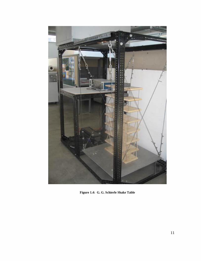
Shake Table: The shake table is the G. G Schierle Shake Table located in the
Masters of Building Science Laboratory consists of a Digital/Analog converter, APS
Dynamics Electro-Seis shaker model 113 and an APS Dynamics amplifier model
114 and a platform suspended from a steel frame. It was originally built in 1981 and
was intended to be used as a teaching tool in the School of Architecture. It has a
steel frame and a wooden platform for the amplifier and the controlling computer.
The shaker is bolted to the base of the frame, and connected to an aluminum
platform with a long bolt. The platform is suspended from the top of the frame with
cables and cross-braced to reduce the introduction of torsion into the model. The
platform has holes drilled 3” on center regularly spaced in a grid, for ease of
securing models for tests. The whole frame is 5’ tall, and 3’ wide.
11
Figure 1.4: G. G. Schierle Shake Table

12
Digital/Analog Converter:
The digital/analog converter is a National Instruments USB-6008 DAC that takes a
digital signal and converts it to a voltage for use with the amplifier.
Figure 1.5 National Instruments USB-6008, Digital Analog Converter,
(http://sine.ni.com/nips/cds/view/p/lang/en/nid/14604)

13
Labview 8.0, Student Version: Labview is a graphic programming language sold by
National Instruments. It uses the C programming language in a graphic way to
control testing instrumentation.
Figure 1.6 Labview Interface Front Screen
The next chapter explores the background of seismic events and modeling.

14
Chapter 2: Seismic Forces and Shake Table Analysis
This chapter will cover the following four things: what earthquake and seismic
events are and how they work, how buildings respond to those forces, what the G. G
Schierle Shake Table is, and the previous research at USC using the shake table.
2.1 Faults An earthquake occurs when built up energy is released in a sudden slippage of a
fault. Faults, or cracks in the earth’s surface, occur primarily at the edges of tectonic
plates, large pieces of the earth’s crust. (Fig. 2.1). There are three types of faults:
Normal, Reverse, and Strike Slip Faults (Fig. 2.2).
Figure 2.1: Major Tectonic Plate Boundaries
http://www.cev.washington.edu/lc/CEVIMAGES/global-techtonic-plates.jpg

15
Normal faults are faults where the hanging wall, the side of the fault that hangs over
the fault, moves downward in relationship to the footwall. An example of a normal
fault is the Mid-Atlantic Ridge, a spreading plate boundary.
Figure 2.2: Types of Faulting in the Earth's Crust
http://earthquake.usgs.gov/images/faq/3faults.gif
Reverse Thrust Faults are faults where the footwall moves upward in relationship to
the hanging wall. An example of a reverse thrust fault is the Sierra Nevada Fault
zone, which has caused the Sierra Nevada mountain range in California.

16
Strike Slip faults are the faults most relevant to Southern California. A Strike Slip
fault is a fault in which one side of a fault moves horizontally in relationship to the
other side of the fault typically parallel to the fault. The San Andreas Fault System
that forms part of the boundary between the North American Plate and the Pacific
Plate is a Strike Slip fault. Strike Slip Faults are either Right Lateral Faults,
meaning that one side of the fault moves from left to right in relationship to a viewer
on the opposite side of the fault, or Left Lateral Faults, in which the motion of the
fault moves from right to left in relationship to a viewer on the opposite side of the
fault. See Figure 2.3 for more information on the faults specific to Southern
California.
Figure 2.3: Earthquake Faults in Southern California
http://www.earthquakecountry.info/roots/inline/11839sm.jpg

17
The San Andreas Fault, which is responsible for some of the largest earthquakes in
California’s history, is a left lateral strike slip fault. A rupture on the southern part
of the San Andreas Fault could unleash an earthquake upwards of Magnitude 8.0.
There are no measurements of any earthquakes occurring on the lower part of the
San Andreas Fault. The last known earthquake was the 1857 Fort Tejon Earthquake,
with a recorded Modified Mercalli intensity from X to XI, with a peak ground
acceleration of more than 0.60g, where g = gravity acceleration.. Almost all un-
reinforced masonry buildings were destroyed and the ground badly cracked. There
was a 9-meter displacement, and the fault ruptured for 300 miles, from Parkfield to
Wrightwood, California. Two buildings were destroyed and three were heavily
damaged and considered uninhabitable at the army outpost of Fort Tejon.
2.2 Seismic Forces
When a fault ruptures, it releases a large amount of stored energy. This energy
radiates out from the epicenter, the point on the earth’s surface where the rupture
starts. There are four types of waves. Two of the three are called body waves,
which propagate within a body of rock and radiate out from the epicenter of the
earthquake. The two body waves are P-waves, and S-waves. The third and fourth
types of waves are surface waves, the Love wave and the Rayleigh wave.
P-waves, or primary waves, are the fastest waves, and are compression waves,
meaning they have a push and pull type of motion. P-waves act similarly to sound

18
waves, and move through both solid rock and liquid material. S-waves, or
secondary waves, are shear waves that shear the rock sideways at right angles to its
direction of travel. These waves are slower than P-waves, and cannot travel through
liquid. While P-waves act like sound waves, the S-wave acts more like a sine wave
(Fig. 2.4).

19
Figure 2.4: Types of Earthquake Waves
http://www.darylscience.com/graphics/seiswave.gif

20
When an earthquake occurs, the high-speed P-waves are felt first, in an effect that
rattles windows and can sometimes sound like a sonic boom. The S-waves arrive
with a vertical displacement and a lateral displacement, and are the waves most
likely to damage a building. (Bolt 2004 pg. 20) The time lag between wave arrivals
defines the distance of an earthquake. The distance from three seismic stations
defines the epicenter location. Surface waves travel near the earth surface.
There are two types of surface wave, the Love wave and the Rayleigh wave. Love
waves have a side-to-side movement along the horizontal plane of the earth’s
surface. It has no vertical displacement, and this horizontal shaking is particularly
damaging to a building’s foundations. The Rayleigh wave acts more like an ocean
wave, with an elliptical motion both vertically and horizontally in a vertical plane in
the direction of wave propagation. These surface waves are usually much slower
than the body waves, and in an earthquake, the first moments of shaking are body
waves, followed then by Love waves, which are faster than Rayleigh waves.
2.3 Building reaction to Seismic Forces
Typically, an earthquake can cause four types of damage to a building. A building
can collapse, which can result in the total loss of the building and possibly the lives
of the occupants. A building can suffer structural damage, which leaves the building
standing, but unsafe, and either results in the eventual demolition of the building or
expensive remediation costs to repair the structural damage. A building may also

21
suffer non-structural damage to walls, water pipes, windows, and so forth. These
costs can be expensive to repair, but are preferable to losing lives. Non-structural
damage usually amounts to over 70 percent of total damage (Schierle, 2001, p.1-1).
Lastly, a building might suffer damage to the contents inside, which result from
objects not being properly anchored to walls or otherwise properly secured.
(Congress 1995 pg. 8)
Engineers and architects hope that a building in a seismically active area would
suffer minimal damage, but of the four types, a designer would prefer cosmetic
damage to structural damage or collapse, in an effort to preserve life safety. Of
course, architects would prefer no damage, but due to the nature of seismisivity,
earthquakes are unpredictable, vary in terms of magnitude, strength, period, and
peak ground acceleration. No two earthquakes are alike, and the effects of
earthquake strength can still surprise engineers and seismologists.
22
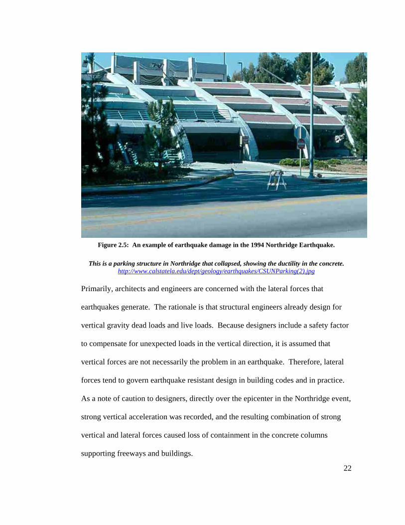
Figure 2.5: An example of earthquake damage in the 1994 Northridge Earthquake.
This is a parking structure in Northridge that collapsed, showing the ductility in the concrete. http://www.calstatela.edu/dept/geology/earthquakes/CSUNParking(2).jpg
Primarily, architects and engineers are concerned with the lateral forces that
earthquakes generate. The rationale is that structural engineers already design for
vertical gravity dead loads and live loads. Because designers include a safety factor
to compensate for unexpected loads in the vertical direction, it is assumed that
vertical forces are not necessarily the problem in an earthquake. Therefore, lateral
forces tend to govern earthquake resistant design in building codes and in practice.
As a note of caution to designers, directly over the epicenter in the Northridge event,
strong vertical acceleration was recorded, and the resulting combination of strong
vertical and lateral forces caused loss of containment in the concrete columns
supporting freeways and buildings.

23
2.4 Model Analysis
Model Analysis is the use of physical or computer models to test shaking or
vibration of an object. Architects and engineers use equations defined by codes to
determine the resonant period of a structure, which is useful to know because a
building will suffer the most physical damage during a seismic event that has the
same frequency as the resonant building frequency. If models are used they must
have similitude to the actual structure that is being studied. A model is said to have
similitude with an actual structure if it has similar geometry, dynamic properties,
and period. Geometric similarity means that the model is a scaled down version of
the actual building, in the same shape. Dynamic similarity means that the ratios of
all forces acting on the building are consistent.
2.5 Shake Tables
Prior to the invention of the seismograph in 1880, there was no way to accurately
test a seismic event. With the invention of the Richter Scale in 1935, there was a
way to measure and compare earthquakes. In the aftermath of the 1906 earthquake
in San Francisco, earthquake research in the United States of America was pushed to
the forefront of geologic studies in California. Two universities in the San Francisco
area, Stanford University and the University of California, Berkeley made major
research gains documenting the effects of the earthquake and the aftermath thereof.

24
2.6 G G Schierle Shake Table Because architects are primarily concerned with the lateral forces added to a
building in a seismic event, the University of Southern California Chase Leavitt
Graduate Building Science Program has a shake table to visually analyze the effects
of a seismic event to a building model. The Schierle Shake Table is a one-degree of
motion shake table, built by Professor Schierle and students. The shake table
includes:
• Steel frame
• Computer
• Suspended aluminum shaker platform
• APS systems Electro-seis 113 shaker component
• Digital/analog converter
• Amplifier component is Model 114
The Schierle Shake Table accepts electronic input via a digital analog converter,
which is a component in the controlling computer. The amplifier takes +/- 2 volts
from a digital/analog converter and modulates the voltage up to 220 volts,
maximum, and 4 amperes are amplified to 6 amperes. Using Labview 8.0, Student
version, from National Instruments, Inc. to input the data and control the output
voltage, one can send actual earthquake waveform data to the shaker to simulate
building response to the seismic event.
25
Using a shake table for modeling building response during a seismic event is useful
to both teachers and students trying to grasp how structures respond to strong lateral
forces. Students can see the deflection in a model, and see the inflection points in
columns. If one uses fabric in the model to simulate walls, a student can see actual
shear forces acting on the fabric. With shake table simulation students see a
visualization of the forces to help understand the building response.
2.7 Previous Work at USC
Professors G. Goetz Schierle, James Ambrose, and Dimitri Vergun, and students
have previously used the shake table to test models under seismic forces.
The theses regarding the shake table in Professor Schierle’s possession are:
H Iriano (1988) Response of High-rise Structures to Lateral Seismic Ground
Movements S Chong (1993) Investigation of Seismic Isolators as a mass Damper for
Mixed Use Buildings
Chong’s Thesis was the last to use the shake table.
The shake table stopped working sometime thereafter.
The testing was thorough, but lacks the specific information on the shake table to
use to restore it. More thorough documentation on the testing equipment would
have been helpful to the restoration of the shake table. However, the notes on model
building were thorough and helpful.

26
No other work mentioning the Shake Table at USC was available.
However, shake tables have been used before in academic environments. The
Network for Earthquake Engineering Simulation (NEES) at Berkeley, California,
first built their large scale shake table in 1972. This table is 20’ x 20’, and has a 3
degree range of motion. It may be used to subject structures weighing 100,000 lbs
to horizontal accelerations of 1.5g. (http://eerc.berkeley.edu/lab/earthquake-
simulator-lab.html). A 3 degree shake table is more accurate than the 1 degree of
lateral motion, because earthquakes cause 3-degree motions that a 1 degree shake
table cannot simulate.
The University of San Diego has the largest outdoor shake table. This shake table is
only a 1 degree of lateral motion shake table, and is 25’ x 40’ in dimension. San
Diego built a 65’ tall concrete building to test that less reinforcing steel is a more
effective strategy in concrete buildings, defined as ductile design required for
concrete structures since 1976. The researchers then tested the building using the
1994 Northridge earthquake event. Their findings support their hypothesis; that
excessive building strength can actually promote poor structural performance and
non-structural damage
(http://www.jacobsschool.ucsd.edu/news/news_releases/release.sfe?id=508). A
National Geographic Special described one critical flaw in their testing in that they
did not take into account the vertical movements in an earthquake, the containment

27
of the concrete in the columns was inadequate, and would have led to the structural
failure of the columns in the actual event (National Geographic 2006).
Small scale testing has occurred at California State University Northridge. Small
scale testing on a shake table is not as accurate as large scale testing because of the
difficulty of scaling down the material properties of actual building materials.
However, small scale testing is good regarding seismic design concepts, such as
shear cracks, building deflection, torsion, and stiffness of a building. For teaching a
conceptual class, such as in an architecture school, such small-scale tests are more
useful because they can be completed in a short amount of time with a minimum of
model building materials.
In the next chapter, a brief introduction to how the G. G Schierle Shake Table
operates and how models can be built to test conceptual ideas will be discussed.

28
Chapter 3: Methodology
Chapter 2 contained the basics of why earthquakes occur, and why building models
to test on a shake table are useful to examine how a building will roughly respond to
a seismic event.
3.1 The G. G. Schierle Shake Table The G. G. S. Shake table is composed of four major components:
• Steel frame
• Computer
• Suspended aluminum shake platform
• Digital analog converter (converts a digital waveform file to a voltage)
• Amplifier (amplifies a small voltage of the digital/analog converter outputs
to a larger current to control the shaker)

29
Figure 3.1 The G. G. Schierle Shake Table.

30
3.2 Amplifier
The amplifier takes a voltage of +/- 2 volts maximum input, and amplifies the
voltage up to +/- 220 volts, maximum output needed to activate the shake table. The
amplifier draws 300 Watts of initial Input Power, and amplifies the current from 4
amps to 6 amps. The amplifier draws 1320 maximum Watts. The amplifier, in
order to work properly, needed to be thoroughly dusted and cleaned, and the fuses
that regulate the input voltage and current needed to be checked and replaced. The
amplifier uses two glass fuses, 250V 4 amp. The current fuse used is an SOC SS2
(Figure 3.2). This fuse is a fusible link made of glass and ceramic to protect against
current surge. The amplifier is connected to the Digital Analog Converter using a
BNC connector. The BNC connector is a type of RF connector used for terminating
coaxial cable (Figure 3.3).

31
Figure 3.2: Picture of fuse used to replace broken fuses.

32
Figure 3.3: A Male BNC Connector used in connecting the digital analog converter to the
amplifier.
http://upload.wikimedia.org/wikipedia/commons/thumb/a/a0/BNC_connector.jpg/639px-BNC_connector.jpg
The amplifier has two circuit boards inside, two capacitors, and a large heat sink and
fan. Using a voltmeter and a multimeter, the digital analog converter sent a test
voltage to the amplifier using the test functions of the digital analog converter to test
the signal in the amplifier. A multimeter is an electronic measuring instrument that
combines several functions in one unit. The most basic instruments include an
ammeter, voltmeter, and ohmmeter. A voltmeter measures only voltage in a circuit.

33
The test function option will automatically pop up on the computer screen when one
plugs the USB cable of the digital analog converter into the USB port.
Figure 3.4: The back of the amplifier
Note the large cooling fan and the circuit that controls the input and output power. In the
multicolored ribbon cable, the orange, yellow, and brown wires seem to handle the input voltage..
Figure 3.4 shows the large cooling fan and the circuit that controls the input and
output power. In the multicolored ribbon cable, the orange, yellow, and brown wires
seem to handle the input voltage. Follow the orange, yellow, and brown wires in the
34
amplifier circuitry to assure that the voltage is properly flowing from the input and
to the output cables. The color-coding seems consistent throughout the amplifier,
however, not all wires were tested and these colors may not be the only wires to
carry voltage and current. There will be a maximum of 42 volts at the capacitors if
the circuitry is working properly. The amplifier needs be grounded to the casing.
With the red probe of the multimeter, switched to voltage, verify that there is 42
volts at the blue capacitors. The black probe should be attached to the case, which is
grounded.
3.3 Digital/Analog Converter
The digital/analog converter used is a National Instruments USB 6008. This device
converts a digital signal, i.e. a waveform, into an analog signal, or a voltage. The
USB device connects to a computer using a USB cable. The device requires a driver
that is available from National Instruments (See Appendix 1). The driver allows one
to test the device and the device is self-calibrating.
3.4 Labview 8.0 Student Version A computer program called Labview 8.0 Student Version was included with the
USB Digital Analog Converter. Labview 8 includes all of the drivers for the testing
instruments provided by National Instruments, Inc. The program includes various
examples to use in creating a controlling program for the G.G.S. Shake Table.

35
Labview uses the “C” programming language in a graphic way to create a
controlling program for the National Instruments components. Please see appendix
2 for a diagram of the program used to control the shake table and other
documentation.
3.5 Shaker The shaker component of the G. G. S. Shake Table has been operational from the
beginning. The internal components, one being a rubber band like piece, might need
replacement in the near future, and the components might need to be lubricated. The
shaker component was thoroughly cleaned and dusted. See Figure 3.5.
Figure 3.5: The Shaker Component of the Shake Table.

36
3.6 Earthquake Data
Earthquake data is acquired from the United States Geological Survey, downloaded
from http://quake.usgs.gov/info/data.html. There are three components to each data
file: peak ground acceleration, peak ground velocity, and displacement.
Displacement is the part of the data file used in Labview to run the shake table.
3.7 Building the Model The model was built based on a prototype building that was instrumented by USGS.
The building has digitized records of many seismic events, and is a good building to
study for testing. Further information about building a model is found in Chapter 5.
3.8 Contingency Plans
Since at the first try, the accelerometers seemed not to be working properly,
measurements of maximum displacement were made by placing a large piece of
paper behind the shake table. A writing implement such as a pencil or crayon was
firmly attached to the model at floor levels corresponding to prototype accelerograph
locations. The pencil had to be in constant contact with the paper to properly record
the displacement. The length of the line on the paper is the maximum displacement
of the building scaled to the model. However, this measurement technique is
questionable because of the torsion of the model while testing. The pencil could not
stay in contact with the paper since the model did not move in a manner parallel to

37
the plane of the paper. The model had torsion because of human error in building
the model, and very slight differences in how the columns were located on the floor
plate. Eccentricities in how the weights were placed on the floor plates might also
have contributed to the torsion in the model.

38
Chapter 4: Fixing the Shake Table
4.1 Original Condition The last time that the shake table was used was in 1993, when Sammy Chong used
the shake table to test mass dampeners. Since then, it has fallen into disrepair. The
controlling computer, a 1980’s IBM PC, would not turn on. The IBM PC had these
components:
• A digital analog converter
• A hard-drive with earthquake files on it
• A program given to the School of Architecture that would run the shake table
The first step towards fixing the shake table was to take the old IBM PC apart, and
see if any of these components were salvageable. When the computer was opened
up, the digital analog converter was not obvious to spot. This component was a PCI
card that connected to the parallel printer port on another board. It was not
salvageable. The hard-drive was also deemed unsalvageable because of the high
possibility that it had rusted solid.
The shake table platform would move manually if the amplifier was on. Thus, the
amplifier and shaker component were assumed to be in working condition, and the
main problem was the computer that had controlled the shake table.

39
4.2 Procedure for Fixing the Shake Table
After contacting the manufacturer of the shake table and amplifier, APS Dynamics,
an operational manual was acquired. This manual did not include a troubleshooting
section, but did include instructions for cleaning the shaker component. The manual
did give some helpful guidelines, such as the amplifier would only accept a +/- 2
volt input.
Using the above guideline, a USB digital analog converter (DAC) was purchased for
the shake table from National Instruments, part number 779051-01. This device had
2 analog outputs, as well as 6 analog inputs and 8 digital inputs/outputs. The digital
component was not important to the function of the shake table at the moment, but
future improvements may want to incorporate such functions. The analog outputs
on the device provide a 0- 5 volt output.
The next step was to connect the amplifier to the DAC. The amplifier had
previously been connected to the controlling computer with a bayonet Neill-
Concelman (BNC) connector, and then an adapter turned the BNC connector to a
26-pin male connector, which plugged into the serial port in the IBM. A BNC
connector was purchased from Amazon.com and screwed into the DAC.
The DAC came with a utility from National Instruments that allowed the device to
be tested, sending out specified voltages from 0-5 volts. After connecting the DAC

40
to both the computer and the amplifier, test voltages were sent to the amplifier, to
see if anything happened at the shaker. Nothing did. Taking apart the amplifier, it
was discovered that one of the fuses was burned out.
Figure 4.1: Block Diagram showing how the shake table components connect to each other.
The fuse, as described in chapter 3, was replaced, and the amplifier and shake table
were dusted using a can of compressed air. Any method for removing dust would be
acceptable, but the can of compressed air was convenient, fast, and did not damage
the equipment. Using a multimeter, all wires and connectors were traced to try and
identify any problematic connections. No obvious flaws were found, except that the
knob on the amplifier does not seem to work properly, and once set, should not be
turned.

41
The amplifier was then connected to the shaker component. The shaker component
moved when a voltage was run through the amplifier. This proved that the amplifier
and shaker were in working order. However, the shaker only had half of its full
range of motion. In order for the shaker to both push and pull, it requires both a
positive and a negative voltage. The DAC could not supply the negative voltage.
See Fig. 4.1 for a diagram of the pin assignments in the connector cable to the
shaker and how the shaker uses both positive and negative voltage for maximum
displacement. The amplifier might not actually be sending a negative voltage to the
shaker. Often a coil with a center tap is used in what is called a push-pull circuit.
Each of the two outputs goes from zero to some voltage, but are out of phase by 180
degrees. When both voltages are equal, the currents in the two halves of the coil
windings are equal, but in opposite direction, so there is no magnetic field. When
one is larger than the other, some of the current does not cancel out so there is a net
magnetic field and the shaker moves. A push-pull circuit can be economical because
a negative voltage is not required in the power supply.

42
Figure 4.2: Shaker Component 3-Pin Connector Diagram
Because the amplifier needed both a positive and a negative voltage, a circuit was
required that would convert a positive voltage into a +/- voltage. This circuit was
designed according to Fig. 4.3 with the help of Joseph Pingree . The circuit uses a
TL082 Operational Amp and several resistors soldered to a PC board. The circuit in
figure 4.3 is the dc-to-dc converter that is used to generate -5 volts from the +5 volts
that is provided by the DAC box. Without it, a separate negative power supply
would have been required.. The PC board was placed in a metal box that was
purchased and modified by the author. See Fig. 4.5 for an image of the metal box
with the DAC and circuitry inside. Fig. 4.6 shows the author soldering the circuit
together. A new BNC connector that mounts directly to the metal box was installed,
and the circuit grounds to the box.

43
Figure 4.3: Circuit designed by Joseph Pingree for DAC.
Figure 4.4: Diagram of the Pin Connections in the TL082 Op Amp that was used to make the
DC to DC converter added to the DAC.

44
Figure 4.5: Image of the DAC inside a custom metal box.
Figure 4.6: The author soldering the circuit to convert a positive voltage to a +/- voltage.

45
After testing that the shake table was indeed working with this new circuit, and had
both a push and pull component, the DAC was tested using an oscilloscope. This
showed that the DAC was sending out a sine wave as expected.
The next component that needed to be added to the shake table was a way to get
digital input back into the computer, to help calibrate the shake table and to record
deflection and movement in the model in a digital way. A MEMS accelerometer
was purchased from Analog Devices Inc. This accelerometer is an ADXL78 MEMS
accelerometer, and is a very small chip. The chip needed to be connected to a PC
board and then connected into the DAC. See Figure 4.7 for a functional block
diagram of the accelerometer.
Figure 4.7: Functional Block Diagram from Analog, Inc.

46
The accelerometer was soldered to a small piece of insulated board. Then wires
were carefully soldered on to the respective pins. See Figure 4.8 for a pin diagram.
These solder connections are very fragile, and the accelerometer was placed into a
small metal box to protect it from unintentional damage.
Figure 4.8: The Pin Diagram for the Accelerometer, from Analog Devices, Inc.
The accelerometer was tested and the output voltages were very small. In order to
reduce added noise to the output signal, an amplifying circuit was required. See
Figure 4.9 for a diagram of the circuit design. Both op amps are part of another
TL082. The potentiometer on the middle left must be adjusted to set the output to
zero when no acceleration is present.

47
Figure 4.9: Circuit design for the amplifying circuit of the accelerometer.

48
The circuit was first designed on a breadboard, and tested before being hardwired.
See Figure 4.10. Then, the circuit was hooked up to an oscilloscope to verify that it
was indeed working. See Figure 4.11.
Figure 4.10: The amplifying circuit tested on a breadboard.

49
Figure 4.11: Oscilloscope, and Joseph Pingree testing the circuit of the accelerometer and
amplifier.
The amplifying circuit required these components:
• 1 PC Board
• 1 20K Ten Turn Trim Pot
• Several Pairs of 6 pin Molex Connectors
• 1 TL082 Operational Amp
• Several colors of stranded 26 gauge wires
50
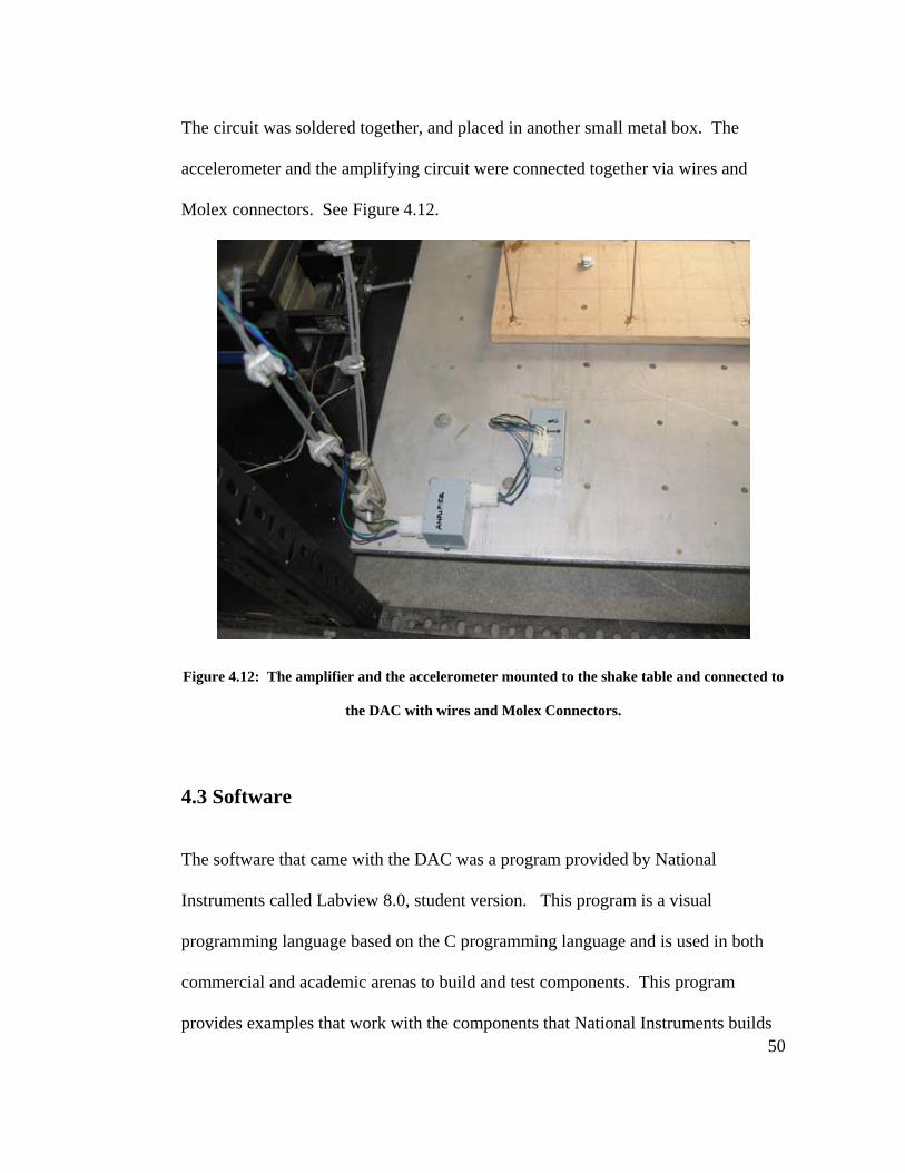
The circuit was soldered together, and placed in another small metal box. The
accelerometer and the amplifying circuit were connected together via wires and
Molex connectors. See Figure 4.12.
Figure 4.12: The amplifier and the accelerometer mounted to the shake table and connected to
the DAC with wires and Molex Connectors.
4.3 Software The software that came with the DAC was a program provided by National
Instruments called Labview 8.0, student version. This program is a visual
programming language based on the C programming language and is used in both
commercial and academic arenas to build and test components. This program
provides examples that work with the components that National Instruments builds

51
and supplies. One such example worked to run a sine wave on the shake table. This
example was then modified to suit the requirements of the shake table. The
controlling software has two components: Front panel and Block Diagram.
Figure 4.13: Labview Front Page
Front page allows the user to change the constraints of the test. See Figure 4.12.
The block diagram is the part of the program that tells the computer, and the DAC,
what to do. A signal is specified, and sent to the DAC. The signal is scaled so that
it will run on the shake table. The signal goes to the shake table and shown on the
Output Graph, runs the shake table, and then a signal is sent back to the computer
via the accelerometer and then shown on the Input Graph. See Appendix A for a
printout of the block diagram.

52
4.4 Problems
Many problems were encountered while restoring the shake table. While designing
each circuit on a breadboard, the circuits were tested using a voltmeter and a power
supply. Before soldering, the circuits worked. After soldering, often the circuits did
not work. This was due in part to the author’s inexperience with soldering, the fact
that the ground in the circuit might not actually be grounded, and that the
connections were not correct. After discovering the initial problem, isolating the
problem was not hard to do with a voltmeter, and some solder connections needed
repair.
The other problem was in the software. While testing, a 3 second delay was
observed. After examining the block diagram in the program, it was discovered that
what was happening was that only the first 1000 samples of data was being run on
the shake table, and then restarting. After removing that part of the program, the
program would run all of the samples of data.
4.5 Troubleshooting If the shake table is not running, check first if the problem is in the computer. Make
sure that the earthquake data file is properly scaled, as data won’t run on the shake
table unless it is inside the +/- 2 amplitude requirement.

53
Make sure all components are properly hooked up and turned on.
If the amplifier is the problem, make sure that the fuses are all intact. The fuses are
located on the back of the amplifier.
Always follow directions in the manual located in the locker attached to the shake
table and clean both the amplifier and the shaker.
If none of the above solves the problem, use a voltmeter and try to isolate the
problem. Turn on the Labview program, and send a voltage through the system.
Open up the DAC box. Check all the connections, to make sure that the voltage is
moving through the system. If it is not, that might indicate a problem in the circuitry
or soldering.
If the problem is in the data coming into the computer, the problem might be in the
accelerometer because of the delicate nature of the soldering, or in the amplifying
circuit. First open up the amplifying circuit box, and turn the screw on the blue trim
pot. The blue trim pot is actually used to set the output of the accelerometer to zero
when there is no acceleration. If that does not work, the problem may be in the
solder connections on the accelerometer, as they are very delicate. If that is the case,
carefully solder the connections back together, being careful not to cause a short.
This can be difficult because the lid of the package is metal.
54
Chapter 5: Building a Test Model
5.1 Types of models already in use
Modeling a building for seismic simulation is a difficult proposition. In order to
know how a building will respond to a seismic event in a definite sense, all of the
material properties of the building must be used in the model. Hence in the field of
earthquake engineering, computer models and full scale testing models of the same
material as an actual structure can best describe a building reaction to a seismic
event.
Computer programs may not be completely accurate, however. Unexpected
discrepancies in the field, like the quality of the construction, would affect the
building’s ability to withstand a seismic force. For example, during the Northridge
Earthquake, several buildings collapsed due to the lack of required nails in plywood
shear walls- nails purposefully left out in order to save money on construction costs.
For that reason, large-scale models built on large shake tables try to incorporate
modern building practices and seismic hazards in a controlled environment. Such
models may also test flawed construction. Large-scale models can give clues as to
how a building will react at an assumed intensity.
55
Small-scale models are useful, for teaching basic principles of earthquake
engineering and structural concepts. Models can be built of wood and piano wire.
Piano wire provides flexibility to allow for flexibility in the columns and show
deflection. Models can also be built of individual brick-like elements to suggest
how an un-reinforced masonry building would react to a seismic event.
Models can be built out of clear acrylic plastic, as long as the floor plates are stiff
and the columns flexible. Models can be made out of paper, to show modal forms
but not seismic behavior. Models can even be built of plaster, but the stiffness of
plaster may not properly simulate seismic behavior.
Forms of failure can be documented using a video camera to capture the initial
failure. Accelerometers can measure maximum displacement, as can paper and
pencil.
5.2 Selecting a Model Type
On a large shake table, to study material reactions to a seismic event, choose a
building material that most closely resembles the material properties of the real
building. The shake table can be used to test types of joints at a larger scale. A
small shake table is not large or strong enough, however, to properly test weld
strength. Thus, small bricks can be stacked together and held together with mortar
to test the reactions of an un-reinforced masonry wall. Plaster with a small gauge
56
wire mesh might replicate a poured in place concrete wall well enough in a small
scale.
To test deflection, modal reactions, bracing, or seismic remediation techniques like
base isolation, models made of wood and wire are acceptable, and easily modifiable.
Base isolators can be tested using rubber pads. Joints should be modeled as they
would be constructed in the prototype building to be tested. For example, if the
prototype building is a moment frame, joints should be fixed in thick floor plates to
prevent any rotation in the joint. If the prototype has a pin joint, then the model
joint should be a pin joint. Bracing can be attached using wood in the shape and
direction of the prototype bracing, or for testing a remedial bracing strategy.
5.3 Modeling a Real Building The important factor of the experiments is to try and match the model’s natural
period of vibration with the period of vibration in the actual building. If the two
match, then all building responses will be similar. If the model’s natural period is
shorter, add more mass to lengthen the period of the model to match the existing
building. If the model’s natural period is longer, reduce the mass to shorten the
period to match that of the existing building.
57
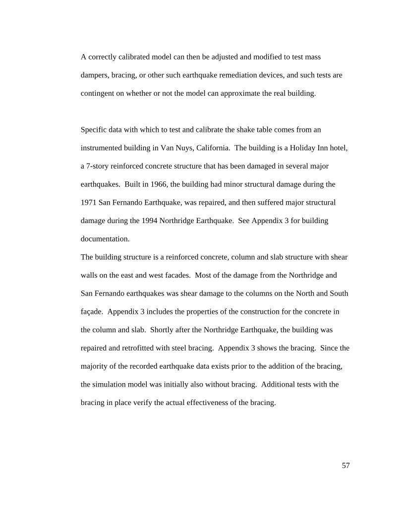
A correctly calibrated model can then be adjusted and modified to test mass
dampers, bracing, or other such earthquake remediation devices, and such tests are
contingent on whether or not the model can approximate the real building.
Specific data with which to test and calibrate the shake table comes from an
instrumented building in Van Nuys, California. The building is a Holiday Inn hotel,
a 7-story reinforced concrete structure that has been damaged in several major
earthquakes. Built in 1966, the building had minor structural damage during the
1971 San Fernando Earthquake, was repaired, and then suffered major structural
damage during the 1994 Northridge Earthquake. See Appendix 3 for building
documentation.
The building structure is a reinforced concrete, column and slab structure with shear
walls on the east and west facades. Most of the damage from the Northridge and
San Fernando earthquakes was shear damage to the columns on the North and South
façade. Appendix 3 includes the properties of the construction for the concrete in
the column and slab. Shortly after the Northridge Earthquake, the building was
repaired and retrofitted with steel bracing. Appendix 3 shows the bracing. Since the
majority of the recorded earthquake data exists prior to the addition of the bracing,
the simulation model was initially also without bracing. Additional tests with the
bracing in place verify the actual effectiveness of the bracing.

58
The data exists for 12 major earthquake events for the building. The Strong Motion
Instrumentation Program of the California Division of Mines and Geology operates
the instrumentation. The records for CDMG, and the other half digitized half of the
earthquakes were digitized at USC. Appendix 3 contains tables of the digitized data
available for the Holiday Inn hotel.
The building has 3 AR-20 accelerographs, which recorded the San Fernando
Earthquake, and a 13 channel CR-1 recording system with a SMA-1 acclerograph,
which recorded all earthquakes from the mid 1970’s to 1994. Figure 5.1 shows the
locations of each recording channel in the building.
Figure 5.1: Locations of the CR-1 recording system in the Van Nuys Building. Image credited
to Prof. Trifunac at USC.

59
The shake table was set up to simulate only the lateral ground motion under the
building in the East-West direction, which was assumed to be the least complicated
direction to study. The data from Channel 16 was used, as an assumption that the
data was the actual ground motion. Thus, the data received back with the
accelerometer would roughly match the actual data taken from the upper stories.
The accelerographs of the upper floors and the roof are for comparison of the model
and shake table to the actual response of the building. The data set used for the
calibration testing was the Northridge Earthquake.
5.4 Symbols The following symbols and definitions shall be used to determine the constraints of
the model.
A= cross sectional area.
D= diameter.
E= Modulus of Elasticity.
I= Moment of Inertia.
L= Unbraced Length of the column or beam.
M= Bending Moment.
P= Axial Load.
R= Radius of Gyration.
T= Period.

60
π= 3.14.
∆= Deflection.
Materials for the model: 1. Plywood sheets.
2. Piano Wires
3. Fishing Weights.
5.5 Calculations The plan is of fixed dimension. The piano wire columns of .062” in diameter have a
Moment of Inertia of 7.25*10–7 . The greater the diameter of the piano wire, the
stiffer the modeled column will be. I=πD 4 /64 is the equation for the moment of
inertia for circular steel columns. Euler’s equation, Pcr=π2 EI/L 2 , is used to
calculate the maximum weight that the wire column can carry.
The slenderness ratio is defined as KL/r. KL/r must be less than or equal to 120 for
primary members, and 200 for secondary members. R is the radius of gyration,
which is defined as r=(I/A)1/2 .
When the piano wire was .032” in diameter, the following calculations were made:
I= πD4/64
I= (3.14) * (.032”)4/64
I=51.47x10⁻⁹
P=(3.14)2 * (29,000,000) * (51.47x10-9)/5

61
P=.6 lbs
When the piano wire was .062” in diameter, the following calculations were made:
I= πD4/64
I= (3.14) * (.062”)4/64
I=725.33x10⁻⁹
P=(3.14)2 * (29,000,000) * (725.33x10-9)/52
P=8.3lbs
This is an acceptable maximum weight for the model.
For the prototype building, the moment of inertia for the columns is I=bd3/12.
Therefore, I=14*203/12. I=9,333.333 in3. The Area of the column is 280 square
inches. The compressive strength of the columns are shown in Fig. 5.2.
1st Floor fc'= 5000 psi2nd Floor fc'= 4000 psi3rd Floor fc'= 3000 psi4th Floor fc'= 3000 psi5th Floor fc'= 3000 psi6th Floor fc'= 3000 psi7th Floor fc'= 3000 psi
Figure 5.2: Compressive Strength of the Columns in the Prototype Building.
The critical loading using Euler’s equation, P=π2 EI/L 2 for the columns in the actual
building are shown in Figure 5.3.
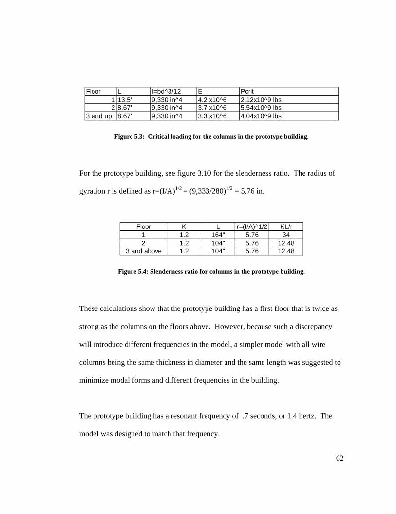
62
Floor L I=bd^3/12 E Pcrit1 13.5' 9,330 in^4 4.2 x10^6 2.12x10^9 lbs2 8.67' 9,330 in^4 3.7 x10^6 5.54x10^9 lbs
3 and up 8.67' 9,330 in^4 3.3 x10^6 4.04x10^9 lbs
Figure 5.3: Critical loading for the columns in the prototype building.
For the prototype building, see figure 3.10 for the slenderness ratio. The radius of
gyration r is defined as r=(I/A)1/2 = (9,333/280)1/2 = 5.76 in.
Floor K L r=(I/A)^1/2 KL/r1 1.2 164" 5.76 342 1.2 104" 5.76 12.48
3 and above 1.2 104" 5.76 12.48
Figure 5.4: Slenderness ratio for columns in the prototype building.
These calculations show that the prototype building has a first floor that is twice as
strong as the columns on the floors above. However, because such a discrepancy
will introduce different frequencies in the model, a simpler model with all wire
columns being the same thickness in diameter and the same length was suggested to
minimize modal forms and different frequencies in the building.
The prototype building has a resonant frequency of .7 seconds, or 1.4 hertz. The
model was designed to match that frequency.

63
5.6 Building the Model
The model was built to a reasonable scale of 1/8”= 1’-0” (1:96) to fit on the shake
table. The shake table surface is 2.5 feet square. The Van Nuys building is
approximately 150’ x 63’. Therefore, the model length is 150/96 = 1.56’. The plan
is of fixed dimension. The columns are of stiff piano wire, of.062” diameter. The
greater the diameter of the piano wire, the stiffer the modeled column will be. Floor
plates are of 1/2” thick plywood of quality grade, to minimize knots and
irregularities in mass. Fishing weights are taped to the floor plates to increase the
mass of the building. Floor plate heights are adjusted up and down, to adjust the
building frequency response on particular floors, and then fixed with epoxy once the
desired frequency is met. (See fig. 5.5).

64
Figure 5.5: Model dimensions, section.
One critical element of the model building is the selection of glue. Use a strong
epoxy. The joints should be clean- apply nothing to the wires or the wood to ease
construction of the model. Wait 24 hours or longer for full strength of the epoxy.

65
5.7 Fixing the Model to the Shake Table
In the metal plate of the shake table, there are holes drilled 3” on center both in the x
and y-axis. Holes are ¼” in diameter. Drill equally spaced holes in the base of your
model that match the holes in the shake table and use ¼” diameter carriage bolts to
bolt the model down to the table. This prevents extraneous shaking due to improper
fixture to the table. See fig. 5.6 for a drawing of the shake table and the holes.
Figure 5.6: Shake Table Plan for Mounting Models (Units in Inches)

66
5.8 Testing
Once the model is built and has the approximate resonant frequency of the prototype
building, place an accelerometer at the location where the actual recording
instrument is on the prototype building. Run the accelerograph from the roof and
gather the data from the accelerometer. Compare the accelerograph from the roof of
the prototype to the data from the shake table, to determine a way to scale
displacement.
After the model has been calibrated and responds like the prototype, build bracing
out of wood and place in the model scaled to the actual prototype. See fig. 5.7. Run
the same record again, and record the displacement. The difference should be
compared to the previous displacement, to see if the bracing that was installed after
Northridge stiffened the building and reduced the amount of deflection on the roof.
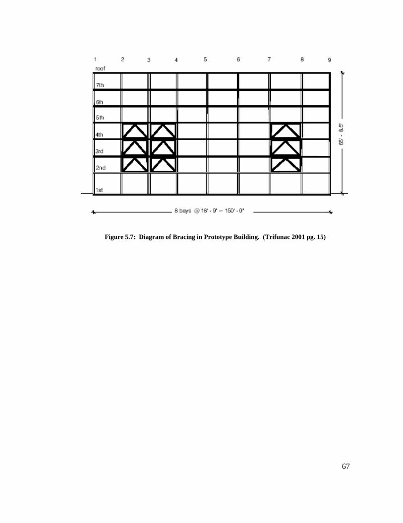
67
Figure 5.7: Diagram of Bracing in Prototype Building. (Trifunac 2001 pg. 15)

68
Chapter 6: Running a shake table test
The following set of instructions is a description of the procedure to be followed for
testing a model.
6.1 Installing the Model
Drill ¼” diameter holes in the model base to attach it to the shake table. Use ¼” in
diameter carriage bolts, 1.5” long as appropriate for the size of the model. Use
washers for spacers if necessary, and use nuts to secure the model.
Place the accelerometer and the amplifying circuit on the model, approximately
where the recording devices are in the prototype building. If the prototype building
had no recording devices, place the accelerometer on the model, in the center of the
top-most floor plate. After each test, move the accelerometer down one level, and
carefully save the data in a file indicative of the location. Affix the accelerometer
with double-stick tape. Carefully install the accelerometer in the direction marked
on the top of the aluminum box. The accelerometer is a single axis MEMS
accelerometer and will only record in the direction marked by the arrows.
A less accurate measuring device can also be used in conjunction with the
accelerometer. Place a large sheet of paper on the white plywood board mounted on
the shake table frame, using masking tape or some other drafting tape. Tape pencils

69
onto the model, in the center of each floor plate, directly in contact with the paper
behind the model. In theory, when the test is run, the pencils will mark the
maximum deflection of the model. In practice, the model has torsion, and the
pencils may not stay in direct contact with the paper. This method does, however,
give a general record of how the model reacted.
A laser instead of pencil would be better to record the model drift.
Assuming that the prototype building has a recorded natural period, the model
should be calibrated to match the prototype period. Run a sine wave in Labview to
match the period of the prototype building. If the model’s natural period is shorter,
add more mass to lengthen the period of the model to match the existing building. If
the model’s natural period is longer, reduce the mass of the model. Labview enters
frequencies in Hertz, so the natural period must be converted into Hertz. One Hertz
is one cycle per second; therefore the frequency of the building is the inverse of the
natural period. See Fig. 6.1 for a screen shot of the Labview program where the
frequency of the prototype building is entered.

70
Figure 6.1: Screen shot of Simulated File Controls
Mass is added to the model in the form of fishing weights. These weights can be
taped on to the floor plates with double-sided tape, which is easy to apply and
remove. The weights are purchased at a fishing store and are made of lead. Lead is
hazardous in large quantities and careful handling is required. See Fig 6.2 for an
image of the lead fishing weights used. Be certain to place the lead at the centroid
of the floor plan, or at least on the central axis in the direction of motion.

71
Figure 6.2: Lead fishing weights used for model testing.
Once the model is properly calibrated, meaning that the model responds with the
strongest shaking at the desired frequency, the model is then ready to test using an
actual earthquake file.
6.2 Selecting an earthquake data file Earthquake data files are recorded in a string algorithm. In computer programming,
a string algorithm is a way to organize data – numbers are separated by spaces,
typically 5 numbers per line. Many programs, including Labview, can read this

72
data. However, this data needs to be reformatted into a single column of data, rather
than five columns of data.
The first step is to choose the earthquake data. Data is available from USGS, but
typically there is a multitude of data for each seismic event. A simpler site to
navigate is COSMOS, the Consortium of Organizations for Strong Motions
Observation Systems. The data is organized by country, state, and recording station.
Any recorded building should be available on the site. U.S. Geological Survey,
California Geological Survey, U.S. Army Corps of Engineers, and U.S. Bureau of
Reclamation, as well as many universities throughout the world run the site.
Download the pertinent data file, and then open the file in Notepad or another word
processor. Some files include several types of data: the best data to use on the
shake table is displacement. Select the displacement data, and copy it into the
Labview program called “Extracting Data”. See Fig. 6.3 for a screenshot of the
program. Follow the instructions to reformat the data into a file format that the
shake table program can use.

73
Figure 6.3: Data Extracting Program
6.3 Verifying Input and Output results A simple test to verify input and output results is to place the accelerometer on the
shake table, input the desired data file, and run the shake table without a model. Run
a sine wave at 1Hertz. The output file, the data file the computer sends to the shake
table, should match the input file on the Labview front page. See fig. 6.4 for a
screenshot of the data display.

74
Figure 6.4: Input and Output graphs
6.4 Running the test
After verifying that the earthquake input and output match, load the earthquake file
in the box shown in Fig. 6.5.
Figure 6.5: Labview File Input
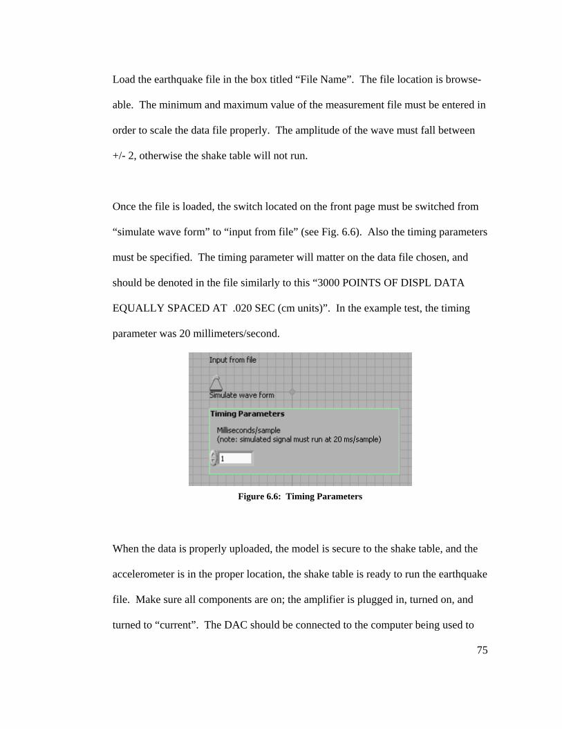
75
Load the earthquake file in the box titled “File Name”. The file location is browse-
able. The minimum and maximum value of the measurement file must be entered in
order to scale the data file properly. The amplitude of the wave must fall between
+/- 2, otherwise the shake table will not run.
Once the file is loaded, the switch located on the front page must be switched from
“simulate wave form” to “input from file” (see Fig. 6.6). Also the timing parameters
must be specified. The timing parameter will matter on the data file chosen, and
should be denoted in the file similarly to this “3000 POINTS OF DISPL DATA
EQUALLY SPACED AT .020 SEC (cm units)”. In the example test, the timing
parameter was 20 millimeters/second.
Figure 6.6: Timing Parameters
When the data is properly uploaded, the model is secure to the shake table, and the
accelerometer is in the proper location, the shake table is ready to run the earthquake
file. Make sure all components are on; the amplifier is plugged in, turned on, and
turned to “current”. The DAC should be connected to the computer being used to

76
control the shake table and the accelerometer should be hooked up to the DAC.
When all the connections have been checked, press the “run” button, which is a
white arrow located in the upper left of the screen.
Figure 6.7: Illustration of "Run" Button
Figure 6.7 shows the arrow button that will start the shake table running. Labview will open up a prompt to save the data file from the accelerometer. Save
the file in an easily accessible location. The data will collect until the “Stop” button
is pressed. See Fig. 6.8 for an illustration of the stop button.
Figure 6.8: The Stop Button

77
The shake table shaking can be documented by using a video camera, and test pencil
or laser in addition to the data from the accelerometer.
6.5 Possible Problems It is possible that during or after repeated tests, the model may become damaged.
This may be due to glue or connection failure, or permanent deformation of
columns. One common sense strategy is to only use the model on the shake table
when calibrating the model or running a test. Excessive shaking may cause damage
to a model. Hot glue or reapplying epoxy glue can help to fix joints that have been
damaged as a stopgap measure, but the best strategy is to build another model when
the first model is too damaged to use.
If the shake table becomes damaged, first check to see that all the connections are
undamaged. The fuses on the back of the amplifier might have broken, and if that is
the case, simply replace the fuses. If the damage is not in the connections or in the
amplifier, contact APS Dynamics in Carlsbad, California, manufacturer of the
shaker unit.

78
APS Dynamics
5731 Palmer Way, Suite A
Carlsbad, California 92120
760-438-4848
The shake table needs to be calibrated so that the data from the shake table can be
published. However, there may be inaccuracies in the shake table data. One that
was noticed was that while running a simple sine wave, the shake table’s
displacement started out small and got larger before settling on about 3.5 centimeters
from it’s natural resting point at 1 Hertz. The shake table did seem to have the same
amplitude in both the positive and negative directions, so the change in amplitude
might have more to do with inertia than an inaccuracy in the shake table.
The shake table should be able to run any desired earthquake file. If the file will not
run, check to make sure that the maximum and minimum values have been properly
input, because improper scaling can cause problems. If the file still does not run,
turn the amplitude knob on the amplifier. This is not recommended for regular use,
as the amplitude knob seems to be problematic. If neither of the above solutions
work, then check to make sure that the file is the correct data. If running a simulated

79
waveform does not work as well, then the problem may be in the shake table itself,
and outside help may be required.

80
Chapter 7: Results and Analysis
7.1 Introduction of Testing The following table is a record of all the tests that were run on the shake table and
how the test was recorded.
Test # Earthquake/Frequency How the Test was recorded Results/Comments
1 5 Hz Video Test recorded push motion of shake table. 9/20/06
2 5 Hz Video Test recorded push/pull motion of shake table 10/11/06
3 1.3 Hz to 5 Hz, adjusted to
2.8 Hz for resonant frequency of model.
Video Testing of variable floor plate height
model and resonant frequency of model. 10/18/06
4 10 Hz to 1.4 Hz Video
Test of fixed floor plates with soft story on first floor. Discovered that soft story added extra frequencies into the model, and thus made it unsuitable for testing.
10/25/06
5 Resonant Frequency Hand Test Video Test to determine resonant frequency of
new model with no soft story. 11/15/06
6 1 Hz Excel/ Notepad Accelerometer Test with Mass on Shake Table 11/29/06
7 1 Hz Excel/ Notepad Accelerometer Test with No Mass on Shake Table 11/29/06
8 1 Hz Excel/ Notepad Accelerometer Test after reattaching the accelerometer 11/29/06

81
9 1.4 Hz Video Test recorded that new model would
resonate at the same frequency of the prototype building. 11/29/06
10 Northridge at Van Nuys, Channel 1 Video Test recorded how the model
responded to Northridge. 12/2/06
11 Northridge at Van Nuys, Channel 1 Paper
Test recorded maximum deflections on Roof, 6th, 3rd, and 2nd floors of model.
12/2/06
12 Northridge at Van Nuys, Channel 1 Paper
Test recorded maximum deflections on Roof, 6th, 3rd, and 2nd floors of model.
12/2/06
13 Northridge at Van Nuys, Channel 1 Paper
Test recorded maximum deflections on Roof, 6th, 3rd, and 2nd floors of model.
12/2/06
14 1 Hz Excel/ Notepad Test recorded the data coming in from the accelerometer to determine if it was
working properly. 12/09/06
15 1 Hz Excel/Notepad Input/Output test- verified 3 times on 1/23/07.
16 1.4 Hz Excel/Notepad Resonant Frequency Calibration 1/25/07
17 Northridge at Van Nuys, Channel 16 Excel/Notepad
Test recorded maximum deflections on Roof, 6th, 3rd, and 2nd floors of model.
1/25/07
18 Northridge at Van Nuys, Channel 16 Excel/Notepad
Test recorded maximum deflections on Roof, 6th, 3rd, and 2nd floors of model.
1/25/07
19 Northridge at Van Nuys, Channel 16 Excel/Notepad
Test recorded maximum deflections on Roof, 6th, 3rd, and 2nd floors of model.
1/25/07
20 Northridge at Van Nuys, Channel 16 Excel/Notepad
Test with bracing on model, maximum deflections on Roof, 6th, 3rd, and 2nd
floors of model. 1/25/07
21 Northridge at Van Nuys, Channel 16 Excel/Notepad
Test with bracing on model, maximum deflections on Roof, 6th, 3rd, and 2nd
floors of model. 1/25/07

82
22 Northridge at Van Nuys, Channel 16 Excel/Notepad
Test with bracing on model, maximum deflections on Roof, 6th, 3rd, and 2nd
floors of model. 1/25/07
Table 7.1: Table of Tests run on the Shake Table
Table 7.1 shows a table of all the tests run on the shake table. Results recorded on
Video will be attached in a supplementary appendix to the thesis. Any results
recorded in Excel and/or Notepad will be shown as a graph in this chapter, as seen in
Table 7.4.
7.2 Verification Tests
Table 7.2 shows the results of tests 6 through 8. The concern was that the
accelerometer was not properly recording the data, and thus that the accelerometer
was not working. It was discovered that the accelerometer was set up to record 3000
data points per second, and thus, the resulting graph was not longer than .01 seconds
worth of data due to human error. The variations in the line of data are a result of
noise transmitted through the long wires into the DAC.

83
Accelerometer Tests 6,7,8
0
1
2
3
4
5
6
7
1 8 15 22 29 36 43 50 57 64 71 78 85 92 99
Data Points
Test after refixing theaccelerometer
Test with old model ontable
Test with no mass on table
Table 7.2: Accelerometer test 6-8.
Floor Location
Maximum Displacement of
Prototype
Maximum Displacement of Model #1
Maximum Displacement of
Model #2
Maximum Displacement of
Model #3 Roof (channel 3) 25.042 cm 13 cm 10.5 cm 14.5 cm
6th Floor (Channel 4) 22.749 cm 11 cm 9 cm 10 cm 3rd Floor (Channel 5) 14.101cm 9.5 cm 7.5 cm 9 cm 2nd Floor (Channel 8) 14.307 cm 9.5 cm 7.5 cm 9 cm
Ground Floor 12.305cm 7 cm 7 cm 7 cm
Table 7.3: Test 11, paper displacement tests
Table 7.3 shows the displacement measurements of the model while running the data
from Channel 1. This data is suspect because the model was oriented in the wrong
direction for the earthquake data. The data is also suspect because the pencil did not
remain in constant contact with the paper throughout the test due to torsion in the

84
model. A laser would have been better with a high speed camera to capture the
results.
Tables 7.4 shows a test of the noise filters that were introduced to the controlling
program to make the input data more clear, and with less extraneous data points.
Test of Noise Filters
00.5
11.5
22.5
1
1227
2453
3679
4905
6131
7357
8583
9809
1103
5
1226
1
1348
7
1471
3
1593
9
1716
5
1839
1
1961
7
Data Points (1000 points = 1 sec)
Am
plitu
de
Accelerometer
Table 7.4: Test of Noise Filters in the Input of the Accelerometer data.
Table 7.5 shows the results of the first Input/Output verification test. A sine wave of
1 Hz was run on the shake table, and these graphs show the data that comes from the
accelerometer mounted on the table. The first test, 15.1, shows that the noise filters
need to be adjusted. The vertical lines every 5000 data points represent a stop point
automatically placed in Labview when it writes the data file, where it places a
marker in the file to denote the timing of the next 5000 samples.

85
The same test was run three times for verification of data input. The data
corroborates the 1 Hz frequency that the shake table was operating at, thus the shake
table seems to be roughly calibrated and responding properly to the wave files.
Tests 15.2 and 15.3 were run with better noise filters, hence the cleaner lines on the
graphs.
Input/Output Verification Test 15
0
1
2
3
4
5
6
7
1
1001
2001
3001
4001
5001
6001
7001
8001
9001
1000
1
1100
1
1200
1
1300
1
1400
1
1500
1
1600
1
1700
1
1800
1
1900
1
Test 3Test 2Test 1
Table 7.5: Input/Output verification test at 1 Hz
Table 7.6 shows the results of three model tests of the model reaction to the 1994
Northridge event, as recorded by Channel 16 of the recording devices stationed in
the prototype building. The accelerometer recorded 68 seconds of data – only 10

86
seconds of greatest reaction is compiled in the figure to condense the data. 10
seconds was also the Northridge Earthquake intense shaking limit. Three tests, with
all variables remaining the same, were run to verify the output results and rule out
the possibility of aberrations. The second and third tests start off the record being
extremely similar, then after a few seconds, the reactions diverge. This is probably
due to the model, and not due to differences in how the shake table ran the file.
Tests 2 and 3 remain similar throughout the rest of the record. Test 1, however, does
not correspond to the last 2 tests, for reasons unknown.
Table 7.6 shows the prototype building’s reaction to Northridge, during the same
recording time as the record used to test the model. The maximum displacement of
the prototype building does not correspond to the data taken from the model. The
actual record of the building does not resemble the data taken from the model, thus
no numerical comparisons between the model and the building are possible.
Table 7.6 plotted the output of the accelerometer vs. time. This is not the same as the
displacement. To calculate the displacement from the acceleration the acceleration
needs to be integrated twice. The acceleration data has a DC offset, thus the mean
of the acceleration must be subtracted before doing the integration. This may explain
why the model data does not look like that from the real building. The comparisons
between accelerations on different floors, or between two different models are still
valid.

87
7.3 Model Testing and Results
Table 7.6: Tests 18, 19, and 20, Roof

88
This graph shows model response to the Northridge event on the roof of the model. The graph shows
that the largest displacement occurred on the roof, although the reason for the variations between
test 1, and tests 2 and 3, are unknown.
Prototype Building Roof Data
-25
-20
-15
-10
-5
0
5
10
15
20
25
110
120
130
140
150
160
170
180
190
110
0111
0112
0113
0114
0115
0116
0117
0118
0119
0120
0121
0122
0123
0124
0125
0126
0127
0128
0129
0130
01
Data Points over time
Drif
t in
CM
Channel 9 Data
Table 7.7: Prototype Building Roof Reaction to Northridge Earthquake 1994
Generalizations correlating the model and the building can be made: the building
had the greatest deflection on the roof. The model had the greatest deflection on the
roof. The model reacted similarly to the prototype building in all of the tests run:
Therefore, anything done to the model in terms of earthquake remediation, like the

89
bracing that was added to the prototype building after the Northridge Earthquake,
should give general indications of how the prototype building would respond.

90
Table 7.8: Tests 18, 19, and 20 5th Floor
This graph shows model response to the Northridge event on the5th floor of the model. The graph shows more correlation between the tests in the initial seconds, but then the displacement values
diverge. The displacement on the 5th floor is less than that on the roof.

91
Prototype Building 5th Floor
-25-20-15-10-505
101520
110
120
130
140
150
160
170
180
190
110
0111
0112
0113
0114
0115
0116
0117
0118
0119
0120
0121
0122
0123
0124
0125
0126
0127
0128
0129
0130
01
Data Points over time
Drif
t in
CM
Channel 10 data
Table 7.9: Prototype Building 5th Floor Reaction to Northridge Earthquake 1994.
Table 7.8 shows a greater correspondence in the early part of the data records. All
three tests match for the first few seconds, and then diverge. The wave amplitudes
differ, but the waves seem to be peaking at similar times. The timing might be an
issue in the record, but the recording of the data is not human controlled, therefore
probably not an issue. The computer should begin recording the input data as soon
as the data is sent out from the computer.
Table 7.9 shows the prototype building’s reaction to the earthquake. Similarly, the
graphs of the model and the prototype do not correspond. The model and the
building cannot correspond unless the model perfectly mimics the actual building,
and since the actual building’s materiality is very different from the model, and the
building has varying stiffness from the ground floor to the roof, as well as eccentric
loads and live loads.
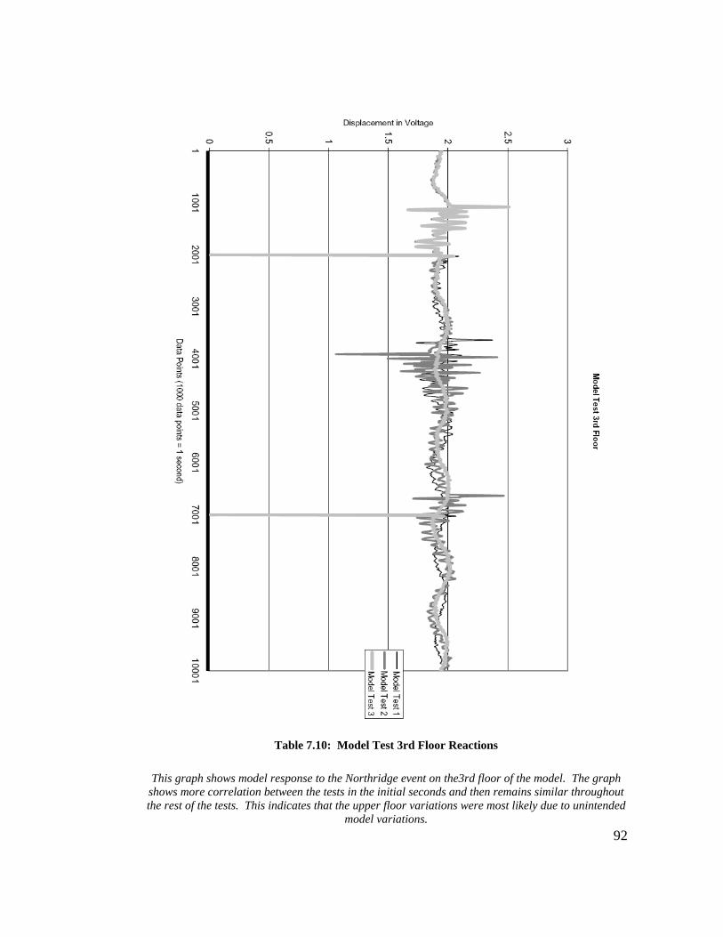
92
Table 7.10: Model Test 3rd Floor Reactions
This graph shows model response to the Northridge event on the3rd floor of the model. The graph shows more correlation between the tests in the initial seconds and then remains similar throughout the rest of the tests. This indicates that the upper floor variations were most likely due to unintended
model variations.

93
Table 7.11: Model Test 2nd Floor
This graph shows model response to the Northridge event on the 2nd floor of the model. The graph shows more correlation between the tests in the initial seconds and then remains similar throughout

94
the rest of the tests. This indicates that the upper floor variations were most likely due to unintended model variations.
Table 7.10 shows the model reactions to the Northridge earthquake file on the third
floor. All three of the files correspond more closely to each other. Thus the model
is probably reacting more regularly at the bottom of the model than at the top of the
building. There might be a more conflicting frequency at the top of the building, or
interference as one waveform hits the top of the model and starts to reverberate back
down.
Table 7.11 shows the model reactions to the Northridge earthquake file on the
second floor. All three tests closely resemble one another in terms of displacement.
The model is reacting predictably, and variations in how the model is built and how
the model responds to the earthquake file are causing the discrepancies at the top of
the model.
After these tests were run, four more tests were run that attempted to model the
bracing of the prototype building during the earthquake retrofit after the damage that
Northridge and the aftershocks caused to the building. The bracing was previously
discussed in Chapter 5. The model bracing was made out of basswood strips, ¼”
wide and approximated the shape of the prototype bracing. The bracing was
fastened with hot glue, and greatly increased the stiffness of the building. While the
bracing reduced the movement of the model in response to the Northridge file, there
is some concern that the bracing would lead to increased damage at the bracing

95
joints due to the stresses that the stiffness would put on the joints. Table 7.12 shows
the model reaction after bracing was introduced, at the roof.
Table 7.12: Model Test of Bracing- roof reaction
This graph shows model response to the Northridge event on the roof of the model, after bracing was introduced. The graph shows that building displacement was reduced 120%, compared to the
building without bracing.

96
Table 7.13: Bracing on the Model- 5th Floor
This graph shows model response to the Northridge event on the 5th floor of the model, after bracing was introduced. The graph shows that building displacement was reduced 120%, compared to the
building without bracing.
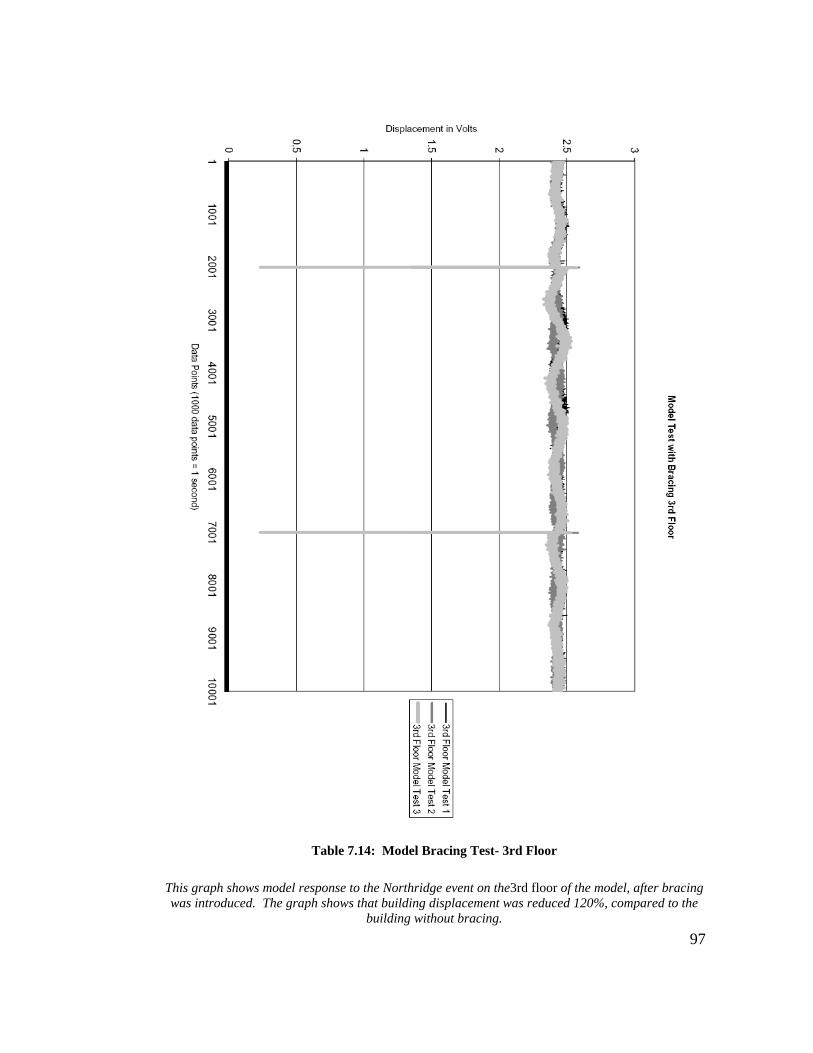
97
Table 7.14: Model Bracing Test- 3rd Floor
This graph shows model response to the Northridge event on the3rd floor of the model, after bracing was introduced. The graph shows that building displacement was reduced 120%, compared to the
building without bracing.
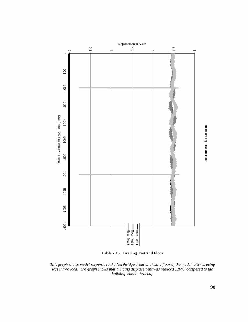
98
Table 7.15: Bracing Test 2nd Floor
This graph shows model response to the Northridge event on the2nd floor of the model, after bracing was introduced. The graph shows that building displacement was reduced 120%, compared to the
building without bracing.

99
The bracing consistently reduced the deflection and dampened the impact of the
earthquake wave. Damage to the building might be reduced due to the lessening of
sharp movements in the building. However, due to the increased stiffness, damage
might be concentrated at the joints of the bracing. There was no damage to the
model after the initial tests.
After running several tests with the bracing on the model, however, there was
damage to the joints where the bracing connected to the floor plates, showing that
either the glue used to fasten the bracing to the model was inadequate, or that the
forces concentrated at the joints was so great to cause damage. This should be
considered while examining the actual building’s structure, and has implications for
the actual connections.

100
Chapter 8: Conclusions
From the test data, it can be seen that the shake table is restored to working order.
The shake table can run both sine waves and earthquake waveforms. When running
a sine wave at 1 Hz, the accelerometer on the shake table sends a 1 Hz waveform
back into the computer.
The test data also shows that the shake table seems to run consistently. This is more
evident in the data files taken from the lower 2nd and 3rd floors, where there is less
variation in the waveforms, and the three tests seem to more closely match. The
shake table also can create repeatable tests.
Each level of the model reacted predictably in each test. There was greatest
deflection at the upper levels and smaller deflection at the lowest level. The model
reacted as expected when bracing was installed on the model. The model’s reactions
are similar to the prototype building’s reactions.
The bracing reduced the acceleration and displacement on all of the floors of the
model and increased the stiffness of the model by 130%. However, increased
stiffness will increase the stress at the joints of the bracing, and might lead to more
future damage in the prototype building. The model’s shaking was greatly reduced
compared to the tests without the bracing. The bracing increased stiffness by 120%.

101
8.1 Correlations to prototype building data
The model can be used to make general conclusions about the behavior of a building
in response to an assumed earthquake. The building had the greatest deflection on
the roof, as did the model. The least amount of deflection in the prototype building
was on the second floor, as in the model. After bracing was added, the building was
stiffer. After adding bracing to the model, the model was much stiffer. While
numerical data taken from the model applied to the building would be questionable,
generalizations about building behavior based on shape and stiffness are valid.
The model cannot be used to make direct numerical conclusions because of
variables beyond the modeling capabilities available in a small-scale model.
Building reaction to a seismic event is dependent on many different variables: soil
type, connection to the foundation, material properties, cladding, partitions, etcetera,
all of which are difficult to model or scale. Modal analysis can occur on a small-
scale model, and generalizations on whether or not an earthquake remediation
attempt will have the desired dampening effect will be possible on a small-scale
model.

102
8.2 Concluding Remarks
The shake table is restored to working order and can be used by the School of
Architecture to teach students basic concepts and building response to seismic
events. The shake table runs consistently and can run an earthquake file.
A model on the shake table can show modal form and building displacement. The
model will react similarly to the prototype building if the model’s resonant
frequency matches the prototype building’s frequency. Earthquake remediation
techniques can be applied to the model to draw general conclusions about the
prototype building. The Van Nuys building’s earthquake retrofit increases the
stiffness of the building, which may lead to more building damage in a future
seismic event.
The University of Southern California’s School of Architecture G G Schierle shake
table can be used in a meaningful way to study a building’s seismic response using
existing seismic data. The G G Schierle Shake Table is an important teaching tool
that is useful to show aspiring architects and engineers how a structure will respond
in a seismic event.

103
Chapter 9: Future Work
9.1 3-Degree of Motion Shake Table
The G. G Schierle Shake Table is a 1-degree of motion shake table, meaning that it
only moves back and forth in one direction. Earthquakes do not move in just one
direction - earthquakes have movement on the x, y, and z-axis. Therefore, in order
to properly study the effects of an earthquake on a building, it is necessary to
incorporate the effect of these movements on the structure. Studying the effects of
only one component of the earthquake is effective for conceptual study but not
specific enough to accurately predict the response a building will have to an
assumed earthquake.
9.2 Different Modeling Techniques
There are many different types of models that can be built to test structures on the
shake table. This thesis only tested one type, the wood and piano wire models
described in Chapter 5. An in-depth study of modeling techniques would be
beneficial to determine whether or not wood and piano wire models are accurate
enough. Acrylic plastic might be an appropriate modeling material, as might metal.
Wood and piano wires do not accurately model the materiality of concrete, and
cannot study masonry buildings.
104
Basswood might be used to model a typical Type V construction project. The wood
pieces can be bought to scale and can be framed out. With wood framing, it might
be possible to get a more accurate small-scale model in terms of material properties
and construction techniques.
Plaster might be used to test poured in place concrete buildings. Actual concrete
might also be used to simulate the material properties of a concrete building. A
study to determine how best to study the materiality of concrete would be quite
interesting and useful to engineers and architects.
Sugar cubes and peanut butter have been used to study masonry buildings in
elementary schools throughout California to build model missions. A similar
modular building material might be able to simulate the dangers of unreinforced
masonry buildings in a seismic event. Small bricks could be made into walls using a
mortar of some kind. It would be important to study the relationship between the
ductility of the “mortar” and the “block” when making conclusions about the mode
of failure.
9.3 Soils Testing
The soil upon which the building is built is a large part of how the earthquake will
affect the building. Softer soils can lead to greater shaking, whereas harder, rockier
soils might reduce the amount of shaking. Earthquake waves travel fastest through

105
dense materials, and in a basin area like Los Angeles, the waves can reverberate in
the soft soils of the basin, reflecting off the rock in the mountain, amplifying the
earthquake waves and causing more damage.
Thus, a way to simulate the soils type that a building is built upon and test the effect
that that has on the building would be very useful. Testing foundation systems
would also be a part of such research. Such testing could occur in a large box
mounted onto the shake table, in which would be the soil type to be tested, some
moisture to hold the ground together, and the model to be tested, anchored into the
soil in the way it was in the prototype. Tests could also study the effect liquefaction
has on a building, and the types of damage that can occur.
9.4 Calibration The shake table needs to be properly calibrated before it can be used to record
numbers for scientific and publishing use. Using the accelerometer, calibrating the
shake table should be a simple prospect. Contact the USC Civil Engineering
Department for more guidance, and perhaps comparison with the already properly
calibrated shake tables in the Civil Engineering Department.
9.5 Better Measurement Devices
The accelerometer is a single axis accelerometer. There are multiple axis
accelerometers, and there are also 6 analog inputs into the DAC. There could be up

106
to 6 accelerometers hooked up to the DAC, taking measurements from 6 different
levels on a model at one time.
Professor Dimitri Vergun recommended a miniature seismograph created using a
rotating drum and a small rotating motor that could be designed to record on paper
the movements of the model. This could be designed and built and implemented for
an alternate way to record model deflection.
9.6 More Earthquake Files
For this thesis, only the Northridge earthquake of 1994 was used for earthquake
data. Earthquake data from all over the world, and from other instrumented
buildings across the United States and from around the world could be tested on the
shake table. The data needs to be found and converted into a form that could be
used by the shake table.
The prototype building studied in this thesis could be used to study how different
earthquakes would affect the same building. Different prototype buildings could
also be studied.
9.7 Earthquake Remediation Strategies

107
Using the same prototype building, different remediation techniques could be
studied to determine whether or not they positively affect the building’s response to
a seismic event. Different bracing types could be tested, as well as the effectiveness
of base isolation. See fig. 9.1 for some examples of eccentric braced frames that
could be tested.
Figure 9.4: Types of eccentric braced frames
(http://www.cen.bris.ac.uk/projects/eqteach97/images/frame8.gif accessed 1/24/07) 9.8 Strategies for use as a teaching tool
The shake table is a valuable teaching tool for use in both the building science
program, both graduate and undergraduate, and in the school of architecture.
Strategies and curriculum should be developed to use the shake table in the
education process. Possible strategies include building different types of models and
running them with different major worldwide earthquakes, such as wood models and
brick models. Another strategy would be to incorporate Architecture students
design models on the shake table to see how the design would withstand earthquakes
typical to the site.

108
There are many further avenues of explorations for the enterprising student using the
shake table as a valuable research or educational tool. The author has only
suggested a few possibilities that were discussed during the course of the Thesis.
The G. G. Schierle Shake Table is a flexible and useful tool that can provide
meaningful results in many fields of research.

109
Bibliography
Bolt, B, 2004, Earthquakes, W. H. Freeman and Company, New York. California University Los Angeles, 2006, viewed 1 November 2006,
<http://www.calstatela.edu/dept/geology/earthquakes/CSUNParking(2).jpg> Chong, L, 1993, Investigations of Seismic Isolators as a Mass Damper for Mixed-
Use Buildings, University of Southern California, Los Angeles. Congress of the United States, Office of Technology Assessment, 1995, Reducing
Earthquake Losses, U.S. Government Printing Office, Washington DC. Crouch, C, Fagan, A, Mazur, E, 2002, Peer Instruction: Results from a Range of
Classrooms, The Physics Teacher, Volume 40, April 2002. Daryl Science 2006, viewed 18 October 2006,
<http://www.darylscience.com/graphics/seiswave.gif> Earthquake Country Alliance 2006, viewed 18 October 2006,
<http://www.earthquakecountry.info/roots/inline/11839sm.jpg> G. G. Schierle, 2003, Northridge Earthquake Field Investigations: Statistical
Analysis of Woodframe Damage, The CUREE- Caltech Woodframe Project, Consortium of Universities for Research in Earthquake Engineering, Richmond CA.
Mazur, E, 1995, Understanding or Memorization: Are we teaching the right thing?,
Department of Physics, Harvard University, Cambridge MA. Missouri Department of Natural Resources 2006, viewed 20 October 2006,
<http://www.dnr.mo.gov/geology/images/Richter_Mercalli.jpg> Moore, F, 1999, Understanding Structures, The McGraw-Hill Companies, Inc.,
Boston. National Geographic, Anatomy of an Earthquake, viewed Sunday, October 15, 2006. National Instruments, 2006, viewed 26 August 2006,
<http://sine.ni.com/nips/cds/view/p/lang/en/nid/14604> National Oceanic and Atmospheric Administration, viewed Oct. 22, 2006,
<http://www.ngdc.noaa.gov/seg/hazard/slideset/22/22_slides.shtml>

110
Trifunac, M, Hao, T, 2001, 7-storey reinforced concrete building in Van Nuys,
California: photographs of the damage from the 1994 Northridge earthquake, USC Report CE 01-05, University of Southern California, Los Angeles, CA.
Todorovska, M, Trifunac, M, 2006, Impulse response analysis of the Van Nuys 7-story hotel during 11 earthquakes and earthquake damage detection, Structural Control and Health Monitoring, University of Southern California, Los Angeles, CA.
Todorovska, M, Trifunac, M, 2006, Impulse response analysis of the Van Nuys 7-story hotel during 11 earthquakes (1971-1994): one-dimensional wave propagation and inferences on global and local reduction of stiffness due to earthquake damage, USC Report CE 06-01, University of Southern California, Los Angeles, CA.
Todorovska, M, Trifunac, M Ivanovic, S, 1999, Instrumented 7-storey reinforced concrete building in Van Nuys, California: description of damage from the 1994 Northridge earthquake and strong motion data, USC Report CE 99-02, University of Southern California, Los Angeles, CA.
United States Geological Survey 2006, viewed 20 October 2006
<http://earthquake.usgs.gov/regional/states/events/1857_01_09.php>. United States Geological Survey 2006, viewed 20 October 2006,
<http://earthquake.usgs.gov/images/faq/3faults.gif> United States Geological Survey 2006, viewed 28 October 2006
http://earthquake.usgs.gov/regional/states/events/1857_01_09.php University of California, Berkeley, 2006, viewed 1 November 2006,
<http://eerc.berkeley.edu/lab/earthquake-simulator-lab.html> University of California San Diego, 2006, viewed 1 November 2006,
<http://www.jacobsschool.ucsd.edu/news/news_releases/release.sfe?id=508> Washington University, 2006, Viewed on 16 October 2006,
<http://www.cev.washington.edu/lc/CEVIMAGES/global-techtonic-plates.jpg>
Wikipedia 2006, viewed 20 October 2006,
<http://upload.wikimedia.org/wikipedia/commons/thumb/a/a0/BNC_connector.jpg/639px-BNC_connector.jpg>
111
Appendix A : Instructions for Using Labview
Instructions for using Labview. 1. Select the Physical Channel to correspond to where your signal is output on the
DAQ device.
2. Enter the Minimum and Maximum Voltage Ranges
3. Set the loop rate.
4. Run theVI.
5. Stop the VI when desired.
Block Diagram Steps: 1. Create an Analog Output Voltage channel.
2. The Array Data is a sinewave with 1000 points, generates 5 cycles, and has an
amplitude of 2.
3. Call the Start VI
4. Write one data point from the array (modulo indexed to loop count) until the user
hits the stop button or an error
occurs. The loop rate is settable to 1 millisecond.
5. Call the Clear Task VI to clear the Task.
6. Use the popup dialog box to display an error if any.

112
Figure A.1: Labview Front Page

113
Figure A.2: Labview Block Diagram

114
Appendix B: Index of Videos Submitted
List of Videos submitted: Shaker Push-Pull
Shaking (Old Model)
Shaking (Torsion)
Shaking (Soft Story)
Shake Table Verification
Resonant Frequency Shaking 1
Resonant Frequency Shaking 2
Model Hand Test