Segmentation and Evaluation of Fluorescence Microscopy Images
184
Segmentation and Evaluation of Fluorescence Microscopy Images Christophe Restif Thesis submitted in partial fulfilment of the requirements of the award of Doctor of Philosophy Oxford Brookes University July 2006
Transcript of Segmentation and Evaluation of Fluorescence Microscopy Images

Segmentation and Evaluation
of Fluorescence Microscopy Images
Christophe Restif
Thesis submitted in partial fulfilment of the requirements of the award of
Doctor of Philosophy
Oxford Brookes University
July 2006
Abstract
This dissertation presents contributions to the automation of cell image analysis,
in particular the segmentation of fluorescent nuclei and probes, and the evalu-
ation of segmentation results. We present two new methods of segmentation of
nuclei and chromosomal probes – core objects for cytometry medical imaging.
Our nucleic segmentation method is mathematically grounded on a novel para-
metric model of the image, which accounts at the same time for the background
noise, the nucleic textures and the nuclei’s contribution to the background fluores-
cence. We adapted an Expectation-Maximisation algorithm to adjust this model
to the histograms of each image and subregion of interest. A new dome-detection
algorithm is used for probe segmentation, which is insensitive to background and
foreground noise, and detects probes of any intensity. We have applied these
methods as part of a large-scale project for the improvement of prenatal diagnos-
tic of genetic diseases, and tested them on more than 2,100 images with nearly
14,000 nuclei. We report 99.3% accuracy for each of our segmentation meth-
ods, with a robustness to different laboratory conditions unreported before. We
compare our methods with existing methods, which we review in detail. We use
them to study the reliability of telomeric probe intensity in order to differentiate
maternal and fetal leucocytes, and show a promising trend.
We also detail a novel framework for referencing objects, combining references
and evaluating segmentation results with a single measure, in the context of med-
ical imaging, where blur and ambiguity add to the complexity of evaluation. This
framework introduces a novel method called Confidence Maps Estimating True
Segmentation (Comets). We compare this framework to existing methods, show
that the single measure allows intuitive quantitative and qualitative interpreta-
tion of discrepancy evaluation, and illustrate its use for tuning parameters on
large volumes of data.
Finally we explain how our methods were ported to a high performance com-
puting cluster server, based on XML databases and standard communication
protocols, to allow reliable, scalable and robust image processing that can be
monitored in real time.
i

Acknowledgements
First of all, I wish to thank my parents for always being there when I needed
them, from my early stage of thinking about a PhD, till the end of it. I also
thank my brothers Olivier and Cyrille, my sisters-in-law Aurore and Marie, for
their continuous help and support.
I would not have started my PhD without the help of many friends and col-
leagues during my time in Paris, a help which was much needed in a time of
changing my professional and personal life. I thank in particular my almost sib-
lings Carine Babet, Anne Mestre and Guy Muller, my recommenders Julie Le
Cardinal, Patrick Callet and Frederique Itier, the Orsyp gang Prakash Hemc-
hand, Frederic Caloone, Michel Enkiri, Mauro Robbe, Arnaud Lamy, Stephane
and Anne-Sophie Daudigeos, Renaud Fargis, Alain Brossard, Alexandre Balzeau,
Esther Fernandez, Anthony Raison, Olivier Denel and Jean-Michel Breul, my os-
teopath Sam Cohen, and my all-time friends Marie Blanchard, Virginie Prioux,
Segolene Tresarrieu, Jean-Philippe Alexander, Odile Prevost, Cecile Rancon, Ma-
gali Druot and the Skalabites band, Nathalie Alepee, Marie Gelibert and the other
rock’n roll dancers. Many thanks also to the Cambridge gang MengMeng Wang,
Jorge Biaggini, Christophe Beauce and Giamee, who supported me from around
the world.
My time in Oxford has been a wonderful experience. I thank my supervi-
sor William Clocksin, in particular for obtaining my scholarship, and my other
supervisors John Nealon and Phil Torr. I give special thanks to Matthieu Bray
and Tony McCollum, who have been constantly helping and supporting me, es-
pecially during our endless talks at Cleo’s. My housemates and lab-mates have
been a pleasure to live with: Sarah, Tom, Derek and the publishers gang, Car-
oline and Ulf, Coco, Jess, Yue, Minhue, Tim, Joumana, David, the ‘elder’ PhD
students Christine, Peter, Prem, and the ‘younger’ ones Wee-Jin, Pawan, Push-
meet, Carl, Pratheep, Sammy, Karteek, Chris, Jon. Many thanks to the friends
who brightened my days, in particular to Arnaud, Jose, Cristiana, Anne-Gaelle
and her friends at the pancake parties, Shemi, Roni, Chloe, Ariel and Nevyanne,
trainer Aline and the salsa teachers Rosa, Giles, Lisa, Mark. Teaching has been a
rewarding experience, and I thank in particular Nigel Crook, Anne Becker, Peter
Marshall, Samia Kamal, and the computing department staff for their help and
all my students for their enthusiasm.
Last but not least, I thank my girlfriend Aurore Aquilina, for sharing my life
and supporting me whenever I need it.
ii

To my parents, my brothers, and my whole family,
To Carine Babet, Anne Mestre,
Guy Muller and Matthieu Bray,
To Aurore Aquilina.
iii

Contents
I Introduction 1
I.1 Towards safer and faster prenatal genetic tests 3
I.1.1 Fetal cells in maternal blood . . . . . . . . . . . . . . . . . . . . 3
I.1.2 Fluorescence microscopy . . . . . . . . . . . . . . . . . . . . . . 5
I.1.3 Need for evaluation . . . . . . . . . . . . . . . . . . . . . . . . . 7
I.2 Specifications of the cytometric task 8
I.2.1 Nucleic segmentation . . . . . . . . . . . . . . . . . . . . . . . . 8
I.2.2 Probe segmentation . . . . . . . . . . . . . . . . . . . . . . . . 10
I.2.3 Evaluation of a segmentation method . . . . . . . . . . . . . . . 11
I.3 Contributions and outline 13
I.3.1 Contributions . . . . . . . . . . . . . . . . . . . . . . . . . . . . 13
I.3.2 Outline . . . . . . . . . . . . . . . . . . . . . . . . . . . . . . . 14
II Review of Segmentation Methods for Cytometry 15
II.1 Low-level vision 18
II.2 Watershed 24
II.3 Active contours 28
II.4 Level sets 45
II.5 Other methods 53
II.5.1 Region growing . . . . . . . . . . . . . . . . . . . . . . . . . . . 53
II.5.2 Neural networks . . . . . . . . . . . . . . . . . . . . . . . . . . 54
II.5.3 Region competition . . . . . . . . . . . . . . . . . . . . . . . . . 55
II.5.4 Graph cut . . . . . . . . . . . . . . . . . . . . . . . . . . . . . . 56
III Evaluating the Telomere Intensity in Leucocyte Nu-
clei from Different Individuals 59
III.1 Segmentation of nuclei 61
III.1.1 Model of the histogram of an image . . . . . . . . . . . . . . . . 62
III.1.2 Expectation-Maximisation algorithm for histogram modeling . . 66
III.1.3 Complete segmentation of the nuclei . . . . . . . . . . . . . . . 71
III.1.4 Results and discussion . . . . . . . . . . . . . . . . . . . . . . . 73
iv

Contents
III.2 Segmentation of telomeric probes 76
III.2.1 Dome-finding algorithm . . . . . . . . . . . . . . . . . . . . . . 77
III.2.2 Results and discussion . . . . . . . . . . . . . . . . . . . . . . . 79
III.3 Comparison of telomere intensities 83
III.3.1 Data set and calibration . . . . . . . . . . . . . . . . . . . . . . 83
III.3.2 Results and discussion . . . . . . . . . . . . . . . . . . . . . . . 86
IV Evaluation of a Segmentation Method 91
IV.1 Existing work 93
IV.1.1 Measures for discrepancy evaluation . . . . . . . . . . . . . . . 93
IV.1.2 Combination of multiple references . . . . . . . . . . . . . . . . 95
IV.2 Comets: a novel method of referencing 97
IV.2.1 Encoding a reference with local confidence . . . . . . . . . . . . 97
IV.2.2 Combining multiple segmentations into a single reference . . . . 99
IV.3 Evaluating a segmentation method with Comets 101
IV.3.1 Evaluation of a single segmented object . . . . . . . . . . . . . 101
IV.3.2 Comparison with other measures . . . . . . . . . . . . . . . . . 102
IV.3.3 Evaluation of a segmentation method . . . . . . . . . . . . . . . 104
IV.3.4 Tuning of a segmentation method . . . . . . . . . . . . . . . . . 106
V Discussion and Future Work 111
V.1 Computer Vision 113
V.2 Cytometry 118
V.3 Future Work 120
V.3.1 Usability of nuclei . . . . . . . . . . . . . . . . . . . . . . . . . 120
V.3.2 Comets for parameter tuning . . . . . . . . . . . . . . . . . . . 120
V.3.3 Distinguishing fetal and maternal nucleated erythroblasts . . . 121
V.4 Conclusion 123
Related publications 124
Appendices 126
A Algorithms 126
A.1 Low-level vision algorithms . . . . . . . . . . . . . . . . . . . . 126
A.2 Watershed algorithm . . . . . . . . . . . . . . . . . . . . . . . . 130
A.3 Geometric active contours . . . . . . . . . . . . . . . . . . . . . 131
v

Contents
B Databases for segmentation and evaluation 137
B.1 Original images and input groups . . . . . . . . . . . . . . . . . 138
B.2 Comets references . . . . . . . . . . . . . . . . . . . . . . . . . 139
B.3 Segmentation results . . . . . . . . . . . . . . . . . . . . . . . . 139
B.4 Evaluation of segmentation results . . . . . . . . . . . . . . . . 141
B.5 Statistics on individuals . . . . . . . . . . . . . . . . . . . . . . 142
C Porting image processing to a cluster 143
C.1 Architecture . . . . . . . . . . . . . . . . . . . . . . . . . . . . . 143
C.2 Protocols . . . . . . . . . . . . . . . . . . . . . . . . . . . . . . 145
C.3 Results and discussion . . . . . . . . . . . . . . . . . . . . . . . 147
D Software interfaces for segmentation and evaluation 150
D.1 Defining and visualising Comets . . . . . . . . . . . . . . . . . 150
D.2 Tuning and using a segmentation method . . . . . . . . . . . . 150
D.3 Visualising the processing on a cluster . . . . . . . . . . . . . . 152
D.4 Visualising measures on different individuals . . . . . . . . . . . 153
Bibliography 154
vi

List of Figures
I.1.1 Typical images obtained with the FISH technique . . . . . . . . 6
I.2.1 The main steps of our image analysis tool . . . . . . . . . . . . 8
I.2.2 Variations of nuclei’s appearances . . . . . . . . . . . . . . . . . 9
I.2.3 Variations of nuclei’s concentrations. . . . . . . . . . . . . . . . 9
I.2.4 Variations affecting image histograms . . . . . . . . . . . . . . . 10
I.2.5 Background illumination . . . . . . . . . . . . . . . . . . . . . . 10
I.2.6 Foreground noise in the FITC channel . . . . . . . . . . . . . . 11
I.2.7 Ambiguity in evaluating a segmentation method . . . . . . . . . 12
II.1.1 Image filtering . . . . . . . . . . . . . . . . . . . . . . . . . . . 18
II.1.2 Pyramid of images . . . . . . . . . . . . . . . . . . . . . . . . . 20
II.3.1 Two systems of coordinates at a vertex . . . . . . . . . . . . . . 29
II.3.2 Image forces at an edge and at a vertex . . . . . . . . . . . . . 32
II.3.3 Polar grid used for certain active contours . . . . . . . . . . . . 39
II.4.1 Illustration of a level set embedding function . . . . . . . . . . 46
II.5.1 Image segmented with dynamic graph-cut . . . . . . . . . . . . 56
III.0.2 Two examples of segmented images. . . . . . . . . . . . . . . . 60
III.1.1 Background illumination . . . . . . . . . . . . . . . . . . . . . . 62
III.1.2 Illustration of our model . . . . . . . . . . . . . . . . . . . . . . 64
III.1.3 Illustration of the proportions . . . . . . . . . . . . . . . . . . . 68
III.1.4 Global and local thresholds obtained from a fitted model . . . . 72
III.1.5 The stages of nucleic segmentation . . . . . . . . . . . . . . . . 72
III.1.6 Examples of incorrect segmentations . . . . . . . . . . . . . . . 74
III.2.1 Examples of foreground noise . . . . . . . . . . . . . . . . . . . 77
III.2.2 Dome model . . . . . . . . . . . . . . . . . . . . . . . . . . . . 79
III.2.3 Pixels affected by the presence of another local maximum . . . 80
III.2.4 Examples of domes constructed in regions with noise and with
probes . . . . . . . . . . . . . . . . . . . . . . . . . . . . . . . . 80
III.2.5 Example of a missed probe . . . . . . . . . . . . . . . . . . . . 81
III.2.6 Comparison of probe segmentations . . . . . . . . . . . . . . . . 82
III.2.7 Probe segmentation on foreground noise . . . . . . . . . . . . . 82
III.3.1 Calibrating factors . . . . . . . . . . . . . . . . . . . . . . . . . 86
III.3.2 Calibrated probe intensity and number of probes per nucleus . . 88
vii

List of Figures
IV.2.1 Construction of a Comets : Mathematics . . . . . . . . . . . . . 98
IV.2.2 Construction of a Comets : Example . . . . . . . . . . . . . . . 99
IV.2.3 Combining multiple segmentations with Comets . . . . . . . . . 100
IV.3.1 Shapes used for the comparison of evaluation measures . . . . . 102
IV.3.2 Results of the comparison of evaluation methods . . . . . . . . 103
IV.3.3 Example of segmentation illustrating user and reference viewpoints104
IV.3.4 Results of the parameter tuning experiments . . . . . . . . . . . 108
IV.3.5 Evaluation of our nucleic segmentation and the watershed with
the Comets measure . . . . . . . . . . . . . . . . . . . . . . . . 108
V.3.1 Illustration of the usabilities found by our method . . . . . . . 121
V.3.2 Individual comparisons of Comets results . . . . . . . . . . . . 121
V.3.3 Nucleated erythroblasts . . . . . . . . . . . . . . . . . . . . . . 122
B.1 Basic structure of an XML file . . . . . . . . . . . . . . . . . . 137
B.2 Databases and process flows . . . . . . . . . . . . . . . . . . . . 138
B.3 Reference database . . . . . . . . . . . . . . . . . . . . . . . . . 139
B.4 Output database . . . . . . . . . . . . . . . . . . . . . . . . . . 140
B.5 Evaluation database . . . . . . . . . . . . . . . . . . . . . . . . 141
B.6 Statistics database . . . . . . . . . . . . . . . . . . . . . . . . . 142
C.1 Client-Server architecture: location of the main processes on the
cluster nodes . . . . . . . . . . . . . . . . . . . . . . . . . . . . 144
C.2 Processing times depending on the number of clients running
per node . . . . . . . . . . . . . . . . . . . . . . . . . . . . . . . 148
D.1 Interface to define Comets references . . . . . . . . . . . . . . . 151
D.2 Interface to segment single images . . . . . . . . . . . . . . . . 151
D.3 Interface to visualise the processing on a cluster . . . . . . . . . 152
D.4 Interface to visualise the measures on different individuals . . . 153
viii

List of Tables
II.0.1 Existing segmentation methods applied to cytometry . . . . . . 17
III.1.1 Initial values of the proportions used for the EM algorithm . . . 69
III.1.2 Results of the nuclei segmentation . . . . . . . . . . . . . . . . 73
III.2.1 Results of the telomere segmentation . . . . . . . . . . . . . . . 81
III.3.1 Number of images for each individual in our data set . . . . . . 84
IV.3.1 Parameters to be tuned . . . . . . . . . . . . . . . . . . . . . . 107
IV.3.2 Parameter values in the first experiment . . . . . . . . . . . . . 107
IV.3.3 Parameter values in the second experiment . . . . . . . . . . . . 107
IV.3.4 Parameter values in the third experiment . . . . . . . . . . . . 107
C.1 Protocol for communication opening . . . . . . . . . . . . . . . 145
C.2 Protocol for communication ending . . . . . . . . . . . . . . . . 145
C.3 Protocol for file transfer . . . . . . . . . . . . . . . . . . . . . . 146
C.4 Protocol for the conversion task . . . . . . . . . . . . . . . . . . 146
C.5 Protocol for the segmentation task . . . . . . . . . . . . . . . . 147
C.6 Total processing time . . . . . . . . . . . . . . . . . . . . . . . 147
ix

List of Algorithms
1 General Expectation-Maximisation algorithm: Two versions . . . 67
2 Expectation-Maximisation algorithm for histogram modeling . . . 69
3 Squared Euclidian Distance Transform . . . . . . . . . . . . . . . 129
4 Watershed by Immersion: Outline . . . . . . . . . . . . . . . . . . 131
5 Watershed by Immersion: Preparing Iso-Level h for Processing . . 131
6 Watershed by Immersion: Extending the Catchment Basins . . . . 132
7 Watershed by Immersion: Processing New Markers . . . . . . . . 133
x

Chapter I
Introduction
1

Segmentation is of fundamental importance in computer vision for discrimi-
nating between different parts of an image. In cytometry, segmentation is used
for the delineation of cells and their components, in particular their nuclei and
specific parts of their chromosomes. Our particular interest is in fluorescence
in-situ hybridisation (FISH) microscopy, in which cells are prepared with fluores-
cent probes that bind to given DNA sequences. Improved segmentation methods
could be used for qualitative and quantitative assay of cell samples.
It has been proposed recently that FISH can be used to discriminate mater-
nal from fetal cells in the maternal bloodstream. Automating this idea places
new demands on segmentation techniques and offers new challenges to computer
vision. In this dissertation we present new contributions that offer significant
improvements in automated cytometry.
2

I.1. Towards safer and faster prenatal
genetic tests
I.1.1 Fetal cells in maternal blood
Over the past twenty years, the age at which women become pregnant has been
rising significantly in Western countries. This is known to increase the risk of
genetic disease for the babies. A typical example is the age-related increase of
frequency of Down syndrome [58, 191], due to trisomy 21 (when cells have three
number 21 chromosomes). Thanks to the progress made by research in genetics,
many genetic diseases can be detected during pregnancy [4]. However, current
diagnostic methods require invasive procedures during pregnancy. Two common
examples are amniocentesis and chorionic villus sampling: fetal cells are sam-
pled directly from within the womb. These methods offer reliable results, but
are uncomfortable, time-consuming, and associated with a 1-2% rate of miscar-
riage [4, 59]. Although these methods are widely used, those risks and costs
prevent them from being routinely used on all pregnant women.
Intensive research is done in biology and cytometry to develop non-invasive al-
ternatives to detect genetic diseases in the fetus. A European Commission-funded
Network of Excellence called SAFE (standing for Special non-invasive Advances
in Fetal and neonatal Evaluation) has recently been started to investigate and
develop such alternatives. One of the promising areas of investigation is the au-
tomated recognition of fetal cells in maternal blood. It has been known for a few
decades that a few fetal cells enter the maternal circulation through the placen-
tal barrier [60, 182]. Isolating these cells non-destructively would give access to
complete genetic information about the fetus, from a maternal blood sample.
Two major issues arise. First, these cells have to be discriminated from ma-
ternal cells in a reliable way. Currently, the most informative descriptor is the sex
chromosomes [78]. In case the fetus is male, its cells will contain a Y chromosome,
3

I.1. Towards safer and faster prenatal genetic tests
whereas the maternal cells will contain only X chromosomes. Consequently, this
method cannot be applied when the fetus is female. There is still need for another
discriminant to identify fetal cells within a maternal sample with certainty. Pos-
sible markers, such as telomeres, are under investigation, and our work is part of
this effort. The second issue is that fetal cells in maternal circulation are present
but rare [80]. Depending on the cells’ types, a non-processed blood sample may
contain one fetal cell within 104 to 109 maternal cells [80,99]. Enrichment meth-
ods exist: the sample can be physically filtered, which reduces the concentration
to 1 in 104 or 105 [64]. This still classifies the problem as a rare-event search.
Computer vision can make the detection of fetal cells easier [113], which is also
an application of our work.
Although many types of fetal cells are present in maternal blood, not all can
be used. The main factor distinguishing them is their expected life-time within
the maternal circulation [60]. Because they qualify as foreign body in the mater-
nal fluids, they are targeted by the maternal immune system. The cells with the
shortest lifetimes, on the order of hours [78], cannot be relied on for our work, as
too few would be present. On the contrary, those with the longest lifetimes, on
the order of years [60] or decades [124], cannot be used either: it would be too
difficult to determine their origin in case of multiple pregnancies. The cells chosen
for our work are leucocytes, or white-blood cells. Their lifetime on the order of a
year [60,152], makes them still acceptable for our purposes, as this whole project
is still in a pilot phase. Besides, unlike other cells, effective enrichment methods
are available for leucocytes [64,65]. Thus, leucocytes offer a reasonable trade-off.
Telomeres are repeated sequences of DNA, namely (T2AG3)n, located at the
end of each chromosomes, about ten thousand base pair long [28, 86, 148, 151].
They contain no genetic information, and shorten during cell divisions through-
out the life of an individual [22,63,151]. They stand out as potential discriminants
between maternal and fetal cells for the following reasons. They are proven to
be longer in fetal cells than in maternal ones, by about 30% [148]. Secondly,
marking them does not alter the genetic material of a cell, which can still be
fully investigated afterwards. Finally, specific markers and techniques exist to
tag telomeres and visualise the results [6,86,112], using Fluorescence in-situ Hy-
bridization (FISH), detailed in the next section. These theoretical reasons still
have to be tested quantitatively [128, 139].
Another issue affects the study of fetal cells in maternal circulation. As the
environmental conditions in the maternal blood are very different from those in
the womb (e.g. the oxygen pressure is 10 times higher in the maternal circula-
tion [5]), and since the immune system is targeting them, fetal cells are physically
affected when they pass the placental barrier. Although it does not affect their
4

I.1. Towards safer and faster prenatal genetic tests
genome, it alters their physical properties. As a result, they cannot be easily
cultivated in vitro, unlike other cells [60]. Without cultivation, they cannot be
prepared and imaged during metaphase, when chromosomes separate before cell
division. They have to be imaged as they were in the sample, in interphase.
Many studies of telomeric length assessment have been published using cultured
cells [6, 86, 112, 183]. The clear separation of chromosomes during metaphase
helps the analysis of genes and telomeres and its automation with computer vi-
sion [128, 139]. In particular, quantitative FISH (Q-FISH) [138], which can be
used to evaluate telomeric length, requires intact metaphase spread [151]. How-
ever, previous work based on metaphase cannot be applied in our context. A
significant difference between the two phases is the arrangement of chromosomes
within the cells. During metaphase, the nucleus border vanishes, and chromo-
somes are clearly distinguished in X-shapes and occupy the whole cell. In inter-
phase though, they are wrapped within the nuclei. They can still be used for
diagnostic purposes: about 70% of chromosomal abnormalities can be detected
in interphase cells [60].
An application of our work is to evaluate whether quantifying telomere length
based on FISH image analysis provides a good discriminant between fetal and
maternal cells, in the case of uncultured interphase leucocytes.
I.1.2 Fluorescence microscopy
Fluorescence is a physical property of some specific materials. When illuminated
at specific wavelengths, usually in the ultraviolet (UV) domain, i.e. between 100
nm and 400 nm, fluorescent materials emit light back, at lower wavelength, usu-
ally in a specific portion of the visible spectrum (e.g. blue, red, green). This
phenomenon is well described by quantum physics: the illumination excites the
material, which progressively relaxes to its original non-excited state. The final
part of the relaxation causes the emission of photons, at a lower energy than the
excitation.
Fluorescence has been widely used as a marker in various fields, from physics,
mineralogy, to biology and cytometry, as early as the 1930s. Fluorescent markers
have been developed for specific cells, parts of cells, nuclei and chromosomes.
In our context, we are interested in visualising two types of objects: nuclei and
telomeres. Two specific markers exist for them. Nuclei can be stained thoroughly
with diamidinophenylindole (DAPI), a fluorescent marker that emits blue light
(maximum of emission at 461 nm [25]). Telomeres can be marked with fluores-
cein isothiocyanate (FITC), which emits green light (maximum of emission at 519
nm [25]). These markers can be attached to the cells’ components with hybridisa-
5

I.1. Towards safer and faster prenatal genetic tests
Figure I.1.1: Three typical images obtained with the FISH technique.
tion: they complement specific DNA and other chemical sequences, and can thus
chemically attach to chosen specific places, such as telomeres and nuclei. This
technique is called Fluorescence in-situ Hybridisation (FISH): the fluorescence
observed is emitted at the place where the hybridisation happened. Details on
the FISH techniques and applications can be found in [25, 95,113].
Fluorescence microscopy differs from classic optic microscopy. In classic mi-
croscopy, the sample to visualise is placed between a source of visible light and
the observer. The light is either absorbed by or transmitted through the sam-
ple. Fluorescence microscopy follows the following principle. A high-intensity UV
light is directed at the sample; the fluorescent markers in use emit light at spe-
cific visible wavelengths; these signals are then observed through adapted filters.
The fluorescent signals obtained are recorded on a charge-coupled device (CCD)
camera, resulting in as many grayscale images as the number of filters used. In
our case, each sample is imaged twice, one in the blue domain for the nuclei, and
one in the green domain for the telomeres. To account for the volume of the
objects, the sample is imaged at fields of view of different depths, distant by 50
nm. The results are averaged to define the final image. Typical reconstructed
and coloured images are shown in Figure I.1.1. Incidentally, in the wavelength
domains used for imaging, the objects imaged are actually sources of light.
The objects in the image are to be analysed in the following way. The nuclei
have to be delineated, or segmented, and their telomeric contents evaluated. This
requires the segmentation of the green signals visible inside them. Although these
signals are attached to telomeres, some telomeres may be unattached to FITC
material and vice versa. For this reason, we will refer to the small bright green
signals as probes, not telomeres. Technically, the task consists in segmenting nu-
clei in the DAPI channel, then segmenting the corresponding probes in the FITC
channel, and evaluating the telomeric contents of every nucleus. As we know
beforehand which nuclei are fetal and which are maternal, a statistical study on
the results obtained will indicate whether this protocol enables a sufficient dis-
crimination between maternal and fetal nuclei.
The core of this work lies in the two segmentation steps, one for the nuclei
and one for the probes. Segmentation results are used to evaluate the differ-
ences between the estimated telomere lengths in different individuals. Also, the
6

I.1. Towards safer and faster prenatal genetic tests
segmentation results need to be evaluated as such.
I.1.3 Need for evaluation
Evaluating a segmentation method is at the same time necessary, important, and
ill-posed. It is necessary to rank segmentation results obtained by different meth-
ods, or one method with different sets of parameter values, in order to select a
method or to tune parameters. Although this sounds natural, deciding on a way
to rank results can actually be difficult. Evaluating a method is also important in
order to assess and validate it: this requires to have a quantitative and qualitative
measure of the segmentation results. Here again, deciding on a metric to perform
these measures is not obvious. Finally, evaluation in itself is an ill-posed task.
It refers to different criteria, some of which have various interpretations and are
measured with various metrics.
Recent publications have clarified the different evaluation criteria. In [201],
Zhang describes three types of evaluation, namely analysis, goodness, and dis-
crepancy. Analysis focuses on the algorithm used in a segmentation method, in
particular its complexity, in terms of memory or runtime. This type of evalu-
ation is important to assess the performance of an algorithm, or to implement
optimisation. In our context however, analysis is not the main evaluation re-
quired: runtime, memory allocation or optimisation are secondary for our pilot
study. Goodness evaluates results based on image and object properties, regard-
less of external references. It can be based on intra-region uniformity, inter-region
contrast, or region shapes. These somehow artificial criteria have been used to
reproduce human judgement on the quality of segmentation in itself. They do not
apply in our task however: our goal is not to produce visually pleasing results,
but to accurately segment nuclei and probes. The final criterion by Zhang is dis-
crepancy : this type of evaluation consists in comparing results against references.
It requires prior referencing of the images, and a measure to compare a computed
segmentation against a reference segmentation. This is the evaluation required
in our context. It allows an objective comparison of segmentation methods and
guidelines for tuning a method’s parameters.
7

I.2. Specifications of the cytometric task
In this section we detail the specific requirements and issues of the cytometric
task introduced in the previous section.
As a pilot study, several sets of leucocytes are to be analysed. There are four
sets, each containing two or three populations of leucocytes, separated from each
other: one from a fetus (obtained through cord-blood), one from an adult woman,
and in some sets one from an adult man. Each population, containing several
hundred cells, was processed and imaged with the FISH technique following the
same protocol. One of our tasks is to develop an image processing tool to evaluate
the quantity of telomeres visible in all the images. Given the high volume of data
to process, the tool is required to be fully automated and robust enough to process
all the samples. Figure I.2 shows the main steps of the required processing.
Process each image
in the database
for each individual
-
4. Compute statistics
of the measures
for each individual
1. Segment
the nuclei-
2. Segment the
probes within
the nuclei
-
3. Measure the
intensities of the
segmented probes
Figure I.2.1: The main steps of our image analysis tool.
I.2.1 Nucleic segmentation
Nucleic segmentation consists in localising and delineating all the nuclei present
in each image. Although the protocols followed during the sample preparation
and imaging are consistent, there are unavoidable variations of experimental and
8

I.2. Specifications of the cytometric task
imaging conditions. The following variations have significant impact on the im-
age quality. First, the nuclei show a wide range of appearances, in terms of
sizes, shapes and textures. Figure I.2.2 shows nuclei with different appearances.
In particular, as the nuclei were not cultured, specific processing ensuring the
convexity of nuclei could not be applied: nuclei do not have fixed convexity or
concavity. Second, the concentration of nuclei within an image is not consistent.
Images may contain from zero to a few dozen nuclei. Some nuclei are isolated,
other are close to their neighbours but still distinguishable by eye: we use the
term touching nuclei to describe them. Other nuclei are tightly clustered and
visually undistinguishable: we use the term clustered nuclei. See Figure I.2.3 for
an illustration of those three cases. Finally, another important type of variation
affects the image histograms. The range of pixel intensities within an image is
sometimes restricted to 200 values, or conversely reaches 1,000 values. The his-
tograms’ shapes may show any number of peaks, valleys, and may contain peaks
resulting from saturation at high intensities. Figure I.2.4 presents three different
histograms.
Figure I.2.2: Variations of nuclei’s appearances, in terms of shapes and textures.
Figure I.2.3: Variations of nuclei’s concentrations. Left: isolated nuclei. Middle: touching
nuclei. Right: clustered nuclei.
An important property of the DAPI images results from the nature of the
FISH imaging technique. As explained in the previous section, the nuclei are
imaged as sources of light. When illuminated in their excitation domain, the
DAPI markers emit light in every direction. The optics used in the microscope
filters the direction of light before imaging. However, not all the light collected
comes directly from the nuclei. Part of the light emitted in different directions is
deflected in the medium surrounding the nuclei, and part of it is collected on the
image. This induces a significant increase of intensity in the background regions
9
I.2. Specifications of the cytometric task
Figure I.2.4: Variations affecting image histograms: three examples of histograms with dif-
ferent range of values. Left: compact range. Middle: medium range. Right: wide range with
high-intensity peaks resulting from saturation.
immediately surrounding the nuclei. We call this effect background illumination,
and refers to the background surrounding nuclei as illuminated background. This
phenomenon is illustrated in Figure I.2.5.
Figure I.2.5: Background illumination. Top left: image with three segmented regions: nucleus,
illuminated and non-illuminated background. Right: intensity values along the horizontal line
across the image. The intensity in the illuminated background is significantly higher than in the
non-illuminated background.
I.2.2 Probe segmentation
Once the nuclei have been segmented in the DAPI images, their content is to be
evaluated in the FITC images. The probes they contain appear as small bright
circles. In the same way, the range of intensities vary significantly across images,
due to slightly different imaging conditions.
Another issue affects the quality of the FITC images. As explained above,
the probes are hybridised to telomeres, then the excess non-attached probes are
washed out of the sample. However, this washing cannot be performed perfectly.
Consequently, unwashed probes tend to gather in large clusters, which appear
very bright on the FITC images. We refer to these cluster as foreground noise.
10

I.2. Specifications of the cytometric task
Although it is a relatively rare phenomenon, affecting about one in thirty images,
it has a significant impact on the image processing. When foreground noise
overlaps a nucleus, it hides the attached probes, and might alter the intensity
measures performed to evaluate the telomeric contents: thus it should not be
segmented as probes. An example of foreground noise overlapping a nucleus is
shown in Figure I.2.6.
Figure I.2.6: Foreground noise in the FITC channel: unwashed cluster of FITC probes overlap
a nucleus, thus hiding part of its actual contents.
I.2.3 Evaluation of a segmentation method
As explained in Section I.1.3, the segmentation results have to be evaluated, using
a discrepancy evaluation against references. The results should be quantitative,
in order to rank different segmentation methods or tune one method’s parame-
ters. In addition, there needs to be a qualitative description of the results as well.
We identified four issues related to evaluation in our context. First, segmentation
results need to be presented in more categories than a “correct / incorrect” binary
outcome: there are several ways in which a segmentation result may be wrong.
Possible segmentation outcomes are:
– Correct: the segmented shape is correct, though it might not be a perfect
match for a pre-defined reference on the object.
– Over-segmented: part of the object is missed by the segmentation.
– Under-segmented: conversely, part of the background (or another object) is
wrongly segmented as the object.
– Missed: the whole object is labeled as background.
– Noise: background is labeled as a valid object.
Not all the incorrect results have the same severity. As we are interested in
evaluating the telomeric contents of the segmented objects, over-segmentation will
affect the measures. Under-segmentation is less severe, unless part of an object
is segmented as another object: that would affect the measures for two objects.
A missed object is not significant for our pilot study, where we are analysing
single populations. However, in the long run the method we develop is meant
to identify rare fetal nuclei within a maternal population: missing nuclei would
then be a serious issue. Finally, segmented noise can be identified after the seg-
11

I.2. Specifications of the cytometric task
Figure I.2.7: Ambiguity in evaluating a segmentation method. Left: image with three ref-
erences. Right: same image with five segmented objects. 33% of the references are correctly
segmented by objects, but only 20% of the objects correctly segment references.
mentation, as not containing probes: it is the less severe outcome in our context.
An evaluation method has to account for these different categories. When over-
and under-segmentation occur on the same object, our approach is to classify the
result as the most severe of these two errors.
The second issue concerns the definition of a correctly segmented object. In
our images, objects boundaries span over several pixels, as a result of the follow-
ing imaging features. First, as in other medical imaging fields, partial volume
effect occurs in microscopy: at the border between objects, more than one object
contribute to the pixel intensities. Nuclei are curved objects, and are imaged at
different depths before the final image is constructed. At each depth a nucleus
will appear with a slightly different radius. In the resulting image the nuclei’s
borders will thus be slightly blurred. Secondly, the background illumination de-
scribed above induces intensity smoothing between a nucleus and its surrounding
background, which increases the boundary blur. Finally, although autofocus is
used during image acquisition, some slides may be slightly blurred if the optical
settings are not optimal. All these effects contribute to the visual blur, which
has to be accounted for during the evaluation: there has to be some tolerance
margin, so that segmented objects not perfectly matching a reference may still
be classified as correct.
The third issue we identified is inter- and intra-user variability, and is also
present in other medical imaging fields. Different experts, or one expert at differ-
ent times, may disagree on some parts of the objects’ boundaries, while agreeing
on others. This calls for a way to combine multiple reference segmentations into a
single one. Ideally this process should keep as much expert knowledge as possible.
The final issue lies in the interpretation of evaluation results. Fig. I.2.7 shows
an artificial reference and segmentation output. While one in three references
are correctly segmented, it is also true that only one in five segmented objects
correctly segment a reference. Thus the success rate of that segmentation could
either be 33% or 20%. Similarly, the oversegmentation rate may either be one in
three, or two in five. Published results [66, 143] tend to use the former of those
numbers. Meaningful as it is, this approach does not account well for the amount
of noise segmented as objects, nor for the number of objects oversegmenting one
reference. There is a need to clarify the interpretation of results while presenting
as much data as possible.
12

I.3. Contributions and outline
In this section we list the contributions we have made to provide a working tool
for the tasks presented in section I.1, given the specifications and issues detailed
in section I.2, and we present the outline of this dissertation.
I.3.1 Contributions
In this work we present the following contributions:
1. A novel segmentation method for fluorescent nuclei which is at the same
time automatic, robust and more accurate than previously published work,
achieving a success rate of 99.3% on our data set, containing nearly 14,000
objects. It is based on a novel mathematically grounded model of the
image, and uses an adaptation of the Expectation-Maximisation algorithm
for histogram modeling.
2. A novel segmentation method for fluorescent probes, also automatic, robust
in particular to foreground noise, and which also has a success rate of 99.3%
on our data set. It is based on a novel dome-detection algorithm sensitive
to the local density of local maxima in image values.
3. A novel method of referencing medical images, with efficiently stored local
confidence factors, which can be used to combine multiple references while
keeping more expert knowledge than existing methods, and to evaluate
segmentation results quantitatively and qualitatively, with a single measure.
4. A comprehensive and consistent review of existing segmentation methods
in cytometry, with particular emphasis on their strengths, weaknesses and
improvements.
5. An XML database structure adapted to our cytometric task.
13

I.3. Contributions and outline
6. A detailed case study of porting an image analysis tool to a cluster.
7. Complete working software, developed in Java, to reference medical images,
tune a segmentation method’s parameters, mass process any volume of im-
ages on a cluster, and visualise segmentation and evaluation results, with
consistent interfaces and framework.
I.3.2 Outline
This dissertation is organised as follows.
Chapter I introduces the task at hand, presents its technical specifications and
its challenges as a computer vision problem, and lists our contributions.
Chapter II reviews the state-of-the-art segmentation methods published and cur-
rently used in cytometry, discusses their strengths and weaknesses, and presents
recent improvements, in the light of our cytometric task.
Chapter III presents our novel segmentation methods, for the nuclei and for the
probes. It details their underlying principles and algorithms, and compares them
qualitatively and quantitatively with existing methods.
Chapter IV details our novel method to reference images and evaluate segmen-
tation methods, called Comets. It explains how a reference is built from user
input, how multiple references are combined, and how segmentation results are
evaluated both quantitatively and qualitatively with a single measure. It also
presents a quantitative comparison with existing evaluation methods.
Chapter V discusses the main issues addressed in this work, and lists three future
projects emerging from this work, namely a classification of segmented nuclei in
terms of usability, a further possible use of Comets, and the adaptation of our
segmentation methods for another cytometric task based on other types of cells.
Appendix A details some of the algorithms presented in Chapter II.
Appendices B to D describe the software we developed for segmentation and eval-
uation. Appendix B presents the underlying XML database used, Appendix C
explains the way the image processing was ported to a cluster, and Appendix D
illustrates the user interfaces.
14

Chapter II
Review of Segmentation Methods
for Cytometry
15

In this chapter we present several segmentation methods used in cytometric
applications. We list some of the most popular methods in Table II, published
for the segmentation of specific types of cells.
In this review we deliberately take an application-oriented approach: we re-
view existing methods in the light of our application, described in the previous
chapter. Our approach is different from other published literature reviews on
medical image segmentation. The reviews by McInerney and Terzopoulos [109],
and by Lehmann et al. [90] are method-oriented: they focus on one segmentation
method, active contours, and review its adaptations to several types of medical
images, such as brain or heart scans. In [133], Pham et al. review segmenta-
tion methods for various types of images, but do not mention cytometry. In
application-oriented theses for cytometry, Laak [178] and Wahlby [181] review
two segmentation methods, low-level vision operations and watershed. To the
best of our knowledge, the review closest to our work is in the thesis by Bam-
ford [10], where four segmentation methods for cytometry are reviewed; however,
only the underlying ideas are described, not their actual implementations nor
their improvements.
We detail four commonly used methods, namely low-level vision operations,
watershed, active contours and level sets, and present four less frequent meth-
ods in cytometry, based on region growing, neural networks, region competition
and graph cut. For each method, we detail the original definitions, discuss the
strengths and weaknesses, and present several published improvements.
In this chapter we consider two dimensional grayscale images, and note f(x, y)
the integer pixel value at location (x, y).
16
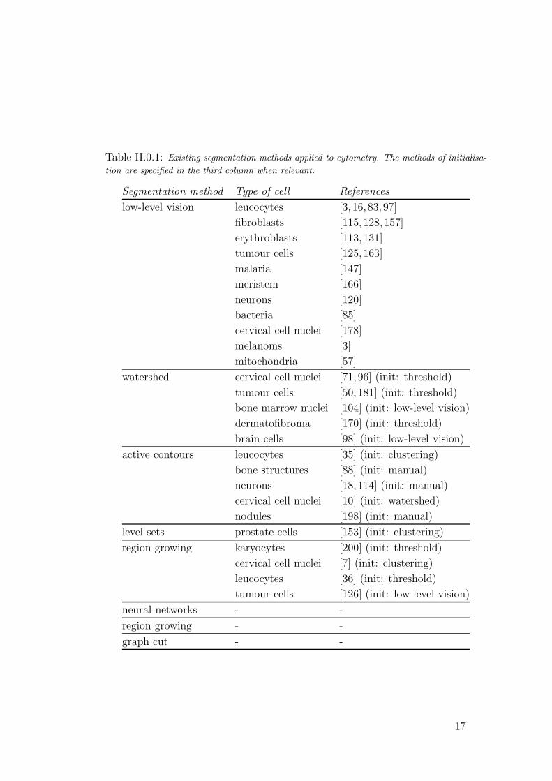
Table II.0.1: Existing segmentation methods applied to cytometry. The methods of initialisa-
tion are specified in the third column when relevant.
Segmentation method Type of cell References
low-level vision leucocytes [3, 16, 83, 97]
fibroblasts [115, 128,157]
erythroblasts [113, 131]
tumour cells [125, 163]
malaria [147]
meristem [166]
neurons [120]
bacteria [85]
cervical cell nuclei [178]
melanoms [3]
mitochondria [57]
watershed cervical cell nuclei [71, 96] (init: threshold)
tumour cells [50, 181] (init: threshold)
bone marrow nuclei [104] (init: low-level vision)
dermatofibroma [170] (init: threshold)
brain cells [98] (init: low-level vision)
active contours leucocytes [35] (init: clustering)
bone structures [88] (init: manual)
neurons [18, 114] (init: manual)
cervical cell nuclei [10] (init: watershed)
nodules [198] (init: manual)
level sets prostate cells [153] (init: clustering)
region growing karyocytes [200] (init: threshold)
cervical cell nuclei [7] (init: clustering)
leucocytes [36] (init: threshold)
tumour cells [126] (init: low-level vision)
neural networks - -
region growing - -
graph cut - -
17

II.1. Low-level vision
Low-level vision consists in processing the image at the pixel-value level, using
very little knowledge of the image contents. It is commonly used in many vision
systems, though often only for pre-processing. In cytometry however, it is often
used to achieve complete segmentation. There are several equivalent definitions
of low-level vision operations [45,46]. For consistency we describe them as kernel-
based filtering processes whenever possible. We present our formalism, and detail
low-level vision operations for noise reduction, shape smoothing, shape extraction,
image transform, and thresholding.
A. Original definitions
Kernel-based filtering: A kernel, or structuring element, may be seen as a
small image. It is defined by its size in pixels, its domain or geometry (e.g. a
disk or a square), its application point (by default its centre) and its shape, i.e.
its values: the kernel is flat if it contains only 0 and 1, non-flat otherwise. We
use the following notations: a kernel k is defined over a domain D(k), indexed
by (i, j). Without loss of generality, we consider D(k) to be square and centred:
D(k) = [−n, n] × [−n, n] for some odd n ≥ 1. Figure II.1.1 illustrates how
to build a filtered image g from an original image f and a kernel k. For some
operations, e.g. dilation, the filtered image g is conventionally noted f symbol k,
where symbol is specific to each operation.
Figure II.1.1: Image filtering.
18

II.1. Low-level vision
Noise reduction: Two ways to reduce the effects of noise are filtering and the
construction of a pyramid of images. Average filtering is achieved by:
kav =1
9
1 1 1
1 1 1
1 1 1
, g(x, y) =
∑
(i,j)∈D(kav )
kav (i, j) · f(x+ i, y + j) (II.1.1)
Gaussian filtering [117] uses the same formula for g, but with non-flat kernels
approximating two-dimensional Gaussian, such as:
1
4
.25 .50 .25
.50 1 .50
.25 .50 .25
,
1
4.76
0 .04 .08 .04 0
.04 .28 .50 .28 .04
.08 .50 1 .50 .08
.04 .28 .50 .28 .04
0 .04 .08 .04 0
(II.1.2)
An alternative is median filtering, where kmed may be 3× 3 or 5× 5:
kmed =
1 1 1
1 1 1
1 1 1
, g(x, y) = median f(x+ i, y + j) , (i, j) ∈ D(kmed)
(II.1.3)
These noise-reducing filters are routinely used before segmentation [3, 125].
Another approach to noise filtering is to build a pyramid of images, from fine
to coarse resolution. It is assumed than images at coarser resolution will only
show the main features of the image, rougher but easier to segment. Pyramid
construction is the basis of segmentation techniques using coarse-to-fine strategies.
Once a pyramid is built, the coarser images are segmented first. The labels found
are then transferred to the next finer scale for improvement. There are many ways
to build a lower-resolution image flow from an image fhigh, which are essentially
sub-sampling methods iterated a few times. Formally, each pixel (u, v) in flow
is computed from a subset of pixels Su,v = (x, y) in fhigh (see Figure II.1.2).
During the coarse-to-fine process, the label of (u, v) will be passed to the pixels
(x, y) ∈ Su,v for refinement. A simple sub-sampling is the following:
Su,v = (2u, 2v), (2u+ 1, 2v), (2u, 2v + 1), (2u+ 1, 2v + 1)flow (u, v) = meanfhigh(x, y) , (x, y) ∈ Su,v
(II.1.4)
Other formulas may be used, such as cubic splines [21, 176]. Gaussian pyra-
mids [23, 149] use wider subsets, and weight the values using Gaussian filtering.
However, the subsets of neighbouring pixels overlap: during the coarse-to-fine
process, the pixels in the overlap will receive two labels.
19

II.1. Low-level vision
Figure II.1.2: Pyramid of images.
Shape smoothing: A shape can be smoothed by smoothing its borders, or by
filling the holes it may contain. Borders can be smoothed by dilation and erosion,
which respectively expand and shrink the shape, or by opening and closing, which
do not affect the overall size of the shape. Any kernel can be used for all these
operations, depending on the smoothing effect expected. The erosion ⊖ and
dilation ⊕ of image f by kernel k are defined as:
(f ⊖ k)(x, y) = minf(x+ i, y + j)− k(i, j), (i, j) ∈ D(k)(f ⊕ k)(x, y) = maxf(x+ i, y + j) + k(i, j), (i, j) ∈ D(k) (II.1.5)
The opening and closing • of f by k are defined as:
f k = (f ⊖ k)⊕ k , f • k = (f ⊕ k)⊖ k (II.1.6)
It is to be noted that opening and closing may alter the connections between
components.
A segmented shape can also be smoothed by filling the holes in it. Holes are
background pixels surrounded by foreground pixels. They can be identified as
background connected components that are not connected to a known background
region, such as the edges of the image. Efficient algorithms to find connected
components are described in [44]. Closing may be used to fill holes as well, but
it can also adversely affect the connections between the segmented components.
An alternative to smooth the borders and fill holes at the same time is the use
of convex hull. In [162], Soille describes methods to compute binary and grayscale
convex hulls efficiently. In short, the binary convex hull of an object is defined as
the intersection of all the semi-planes that contain the object. It is computed by
finding the lines, in several directions, that touch the object without intersecting
it. Incidentally, the difference between an object and its convex hull enhances its
concavities, which may be useful for object recognition. This technique can be
used to detect overlapping convex cells [85].
Shape extraction: A grayscale image can be viewed as a 3D landscape, with
the gray value of a pixel indicating the height of the point. This way, objects
of interests may appear as peaks (sharp mountains), domes (smooth hills), or
20

II.1. Low-level vision
valleys (V- or U-shaped). Such features can be extracted with morphological
operations. The open and close • top-hat transforms of an image f by a kernel
k respectively extract the peaks and the V-shaped valleys in f . They are defined
as:
f k = f − (f k) , f •k = (f • k)− f (II.1.7)
As with opening and closing, any kernel k can be used. The domain and shape of k
actually control the extend and size of the peaks and valleys extracted [45,46,187].
The extraction of domes and U-shaped valleys can be performed with gray-
scale reconstruction [46,179]. The U-shaped valleys of depth h in f are extracted
as the domes of height h in the inverse of f . See Appendix A.1 page 126 for
details on grayscale reconstruction.
Image transform: These operations turn f into an image with the same di-
mensions but whose values are in another domain. Common transforms are gra-
dient extraction (edge map and gradient vector flow), which turns an image into
its derivative, and distance transform, which turns a binary image into grayscale.
Computing the gradient intensity per pixel results in an image called an edge
map. Even though the gradient is mathematically defined for continuous two-
dimensional functions, there are several definitions of gradient when it comes to
image processing. Morphological gradient [46] is defined as the subtraction be-
tween the dilation and erosion of a image, with two kernels ke and ki (usually
ke = ki):
∇ke,kif = (f ⊕ ke)− (f ⊖ ki) (II.1.8)
The term f ⊕ ke is called external gradient, and f ⊖ ki internal gradient. The
resulting value reflects the norm of the gradient, but gives no indication on its
orientation.
Analytical gradients are computed with filters reproducing finite differences.
The same formula:
g(x, y) =∑
(i,j)∈D(k)
k(i, j) · f(x+ i, y + j) (II.1.9)
is used with different kernels, to compute the intensity of the gradient projected
onto different directions. The classic filters used are the Roberts operators (resp.
horizontal, vertical and two diagonals):
0 0 0
−1 1 0
0 0 0
,
0 −1 0
0 1 0
0 0 0
,
−1 0 0
0 1 0
0 0 0
,
0 0 −1
0 1 0
0 0 0
(II.1.10)
21

II.1. Low-level vision
and the Sobel edge-detectors:
−1 0 1
−2 0 2
−1 0 1
,
−1 −2 −1
0 0 0
1 2 1
,
−2 −1 0
−1 0 1
0 1 2
,
0 −1 −2
1 0 −1
2 1 0
(II.1.11)
The same method can be applied to compute Laplacian of images (second deriva-
tive). Using Equation II.1.9, the non-directional Laplacian can be computed with
the kernels [187]:
kLapl4 =
0 −1 0
−1 4 −1
0 −1 0
, kLapl8 =
−1 −1 −1
−1 8 −1
−1 −1 −1
(II.1.12)
The gradient direction can be computed at the same time as its intensity,
resulting in a vector-valued image. One technique is called gradient vector flow
(GVF) [194, 195]. It is detailed in Appendix A.1 page 127.
The distance transform turns a binary image f into a gray-scale image g: each
foreground pixel in f is assigned a grayscale value proportional to the distance
to the closest background pixel. The Chamfer algorithm [187] is a filter-based
method to compute the distance transform in the inside of objects. It can be used
to compute the l0 and l1 distances correctly, with appropriate filters. However,
the l∞ distance can only be approximated: better approximations require bigger
filters and thus more computation time. Besides, it can only be applied to im-
ages where the foreground is surrounded with background. An alternative, fast
algorithm applicable to every image to compute the square of the l∞ distance
exactly is detailed by Felzenszwalb and Huttenlocher [51]. It is reproduced as
Algorithm 3 in Appendix A.1 page 128. During the algorithm, g is scanned only
twice, and at the end, it contains the square of the Euclidian distance transform
of f .
Thresholding: It consists in labeling a pixel as foreground if it is above a
threshold value, and as background if it is below. The threshold value may
be the same for all pixels, or it may be a function T (x, y) of the pixel location,
called a threshold surface. Several thresholds may be used to obtain multi-labeled
segmentation. For robustness, thresholds can be computed using image features,
e.g. its histogram (histogram-based threshold) or using local statistics (space-based
threshold). Sezgin et al. recently published a comprehensive review of threshold-
ing techniques [156]. Two histogram-based threshold methods popular in cytome-
try are Otsu’s and the isodata [104]. They are detailed in Appendix A.1 page 128.
More histogram-based thresholds are presented in [159].
22

II.1. Low-level vision
A simple way to define a threshold surface consists in dividing the image into
smaller tiles [29, 67, 118, 169, 190]. A single threshold value is computed for each
tile; these values are then interpolated over the image.
B. Strengths
The morphological operations described above are straightforward and quick to
implement: they only require image scanning and histogram computations. The
main parameters to tune are the size, geometry and shape of the kernel: their
meaning are intuitive and their effects are easy to perceive. They have linear
complexity, little memory requirements, and thus are fast at runtime. Also, given
the range of functions they perform, they can easily be combined to achieve the
complete segmentation of an image [120]. Finally, even though they are defined
on binary and grayscale images, they can be extended to colour images or stacks
of images, using vector-valued or 3D kernels.
C. Weaknesses
They actually suffer from their simplicity: they can only include very little knowl-
edge about the objects to segment. Thus, they are mostly ad-hoc techniques,
selected and tuned manually to perform well on very specific types of objects,
but have to be rebuilt for other objects. They are little robust to shape and size
variations, as well as intensity variations within an image or across images, which
are all frequent in cytometry images. Finally, as most of them work at the level
of connected components, they are not meant to segment clustered objects.
D. Improvements
Even though the original definitions of the operations can be implemented as such,
the algorithms can be improved, especially for large images. Fast implementations
of the dilation, erosion, opening and closing are described in [30]. Fast algorithms
for grayscale reconstruction are detailed in [179].
23
II.2. Watershed
A. Original definitions
Considering an image as a landscape, the watershed transform can be pictured
as a flooding process. Starting from specific pixels, called markers, water rises
gradually in the landscape. Each valley being flooded is called the catchment basin
of the marker. When two catchment basins come in contact, their connections are
labeled watershed lines. The flooding process continues as if dams were build on
the watershed lines, preventing the actual merging of basins. The process stops
when either the whole image is segmented, or the water level reaches a given height
(the pixels above it are labeled as background). The watershed by immersion
algorithm is reproduced in Appendix A.2, page 131. Mathematical definitions
can be found in [14, 47], along with the links between watershed, skeleton by
influence zones and Voronoi diagrams. Detailed watershed definitions, algorithms
and analyses are in [144].
B. Strengths
A major feature of the watershed is that it is quick to implement, and does
not need any parameter: there is no tuning to do before using it. Regarding its
complexity, it runs in linear time, and its memory requirements are one temporary
image, one array storing sorted pixels, and a queue. As a result it is fast and
cheap.
C. Weaknesses
The main issue is to preprocess the image to produce the correct number of
markers in the right places. Basically, the robustness of the watershed depends
greatly on the robustness of the marker-finding preprocessing. An edge map often
contains too many edges, not fully connected: this creates still too many basins,
24

II.2. Watershed
with possible leaks. The distance transform is convenient to find markers within
convex objects, but finds too many markers within concave objects.
Also, the watershed poorly detects low contrast boundaries [55]: this is in-
herent to the immersion process. Similarly, when a plateau happens to be a
boundary between two basins, it is not properly segmented; however, this seldom
happens with cytometry images.
Finally the watershed transform does not include any prior knowledge on
the objects to segment. This is the inevitable drawback of any parameter-free
segmentation method, and may be a significant issue for robustness.
D. Improvements
The weaknesses mentioned above are well-known, and several methods have been
developed to address them.
Preprocessing: Finding the correct number and location of the markers is cru-
cial for the segmentation results, and has to be done beforehand. Originally all
local minima were used, causing severe oversegmentation. Alternatively, mark-
ers may be placed manually, or found automatically during preprocessing. Two
examples of markers are the h-domes found by geodesic reconstruction [55] (see
Section II.1, Shape extraction), and the maxima of the distance transform on
thresholded images [104]. A combination of them is given by Lin [98]. Using the
distance values D(x, y) and the gradient values G(x, y) (ranging from Gmin to
Gmax), the quantity:
D′(x, y) = D(x, y) · exp
(1− G(x, y)−Gmin
Gmax −Gmin
)(II.2.1)
is assigned to the pixel (x, y). The resulting image is inverted, and has the
following property: it has high values near the boundaries of components, and
also where the gradient is high; conversely, it has low values at the centre of
components and in regions of low variations of intensities. With these properties,
this method can find reliable markers for isolated or slightly touching convex
objects, but not for concave objects.
Postprocessing: over-segmentation can be reduced by merging segmented re-
gions. Using the immersion metaphor, it consists in removing some of the dams
to merge some basins. To select which basins to merge, one way consists in eval-
uating the edges between two neighbouring regions [71]. Various criteria can be
defined, using the range of intensity or gradient values along the edge. Another
way is to measure some similarity between neighbouring regions, and merge the
25
II.2. Watershed
most similar regions. The following issue is to decide when to stop the region-
merging process. This may be done after a fixed number of merges [160], or when
all regions meet some predefined quality criteria, e.g. based on their circularity.
Overall this approaches introduces several parameters, and is often used ad-hoc.
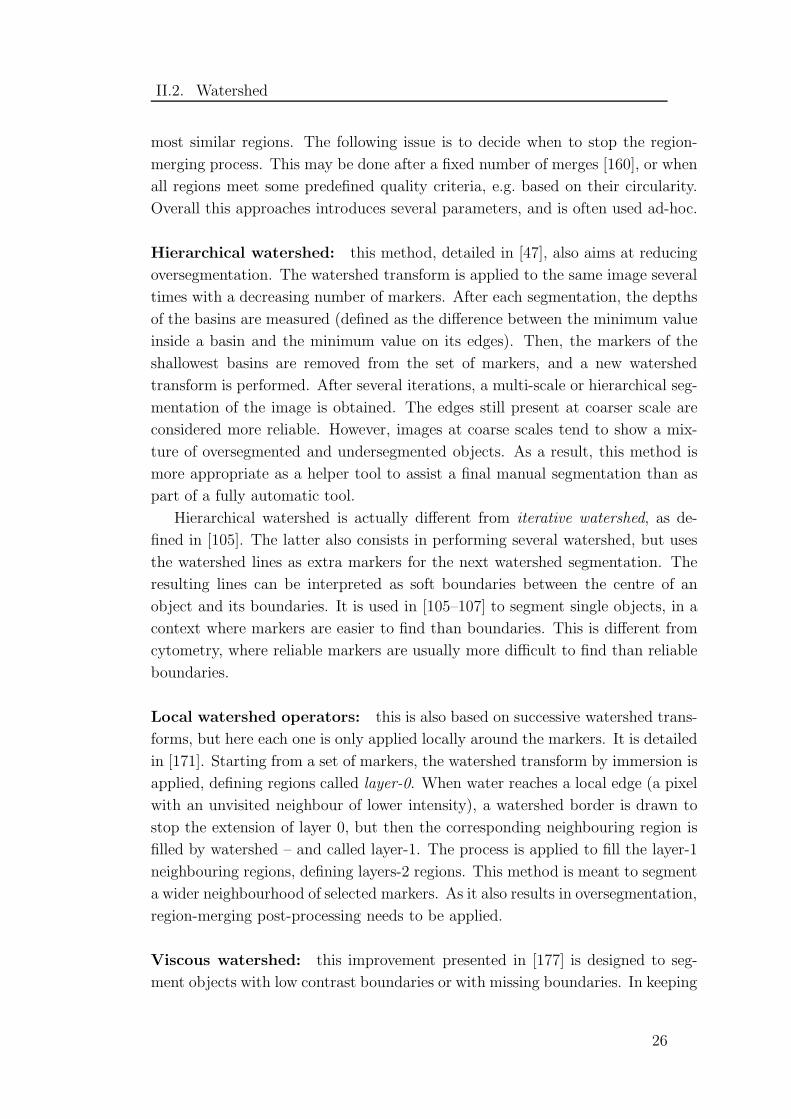
Hierarchical watershed: this method, detailed in [47], also aims at reducing
oversegmentation. The watershed transform is applied to the same image several
times with a decreasing number of markers. After each segmentation, the depths
of the basins are measured (defined as the difference between the minimum value
inside a basin and the minimum value on its edges). Then, the markers of the
shallowest basins are removed from the set of markers, and a new watershed
transform is performed. After several iterations, a multi-scale or hierarchical seg-
mentation of the image is obtained. The edges still present at coarser scale are
considered more reliable. However, images at coarse scales tend to show a mix-
ture of oversegmented and undersegmented objects. As a result, this method is
more appropriate as a helper tool to assist a final manual segmentation than as
part of a fully automatic tool.
Hierarchical watershed is actually different from iterative watershed, as de-
fined in [105]. The latter also consists in performing several watershed, but uses
the watershed lines as extra markers for the next watershed segmentation. The
resulting lines can be interpreted as soft boundaries between the centre of an
object and its boundaries. It is used in [105–107] to segment single objects, in a
context where markers are easier to find than boundaries. This is different from
cytometry, where reliable markers are usually more difficult to find than reliable
boundaries.
Local watershed operators: this is also based on successive watershed trans-
forms, but here each one is only applied locally around the markers. It is detailed
in [171]. Starting from a set of markers, the watershed transform by immersion is
applied, defining regions called layer-0. When water reaches a local edge (a pixel
with an unvisited neighbour of lower intensity), a watershed border is drawn to
stop the extension of layer 0, but then the corresponding neighbouring region is
filled by watershed – and called layer-1. The process is applied to fill the layer-1
neighbouring regions, defining layers-2 regions. This method is meant to segment
a wider neighbourhood of selected markers. As it also results in oversegmentation,
region-merging post-processing needs to be applied.
Viscous watershed: this improvement presented in [177] is designed to seg-
ment objects with low contrast boundaries or with missing boundaries. In keeping
26

II.2. Watershed
with the immersion metaphor, the liquid used is replaced by either oil, for blur,
or mercury, for missing edges. Instead of modifying the watershed implementa-
tion to simulate viscous immersion, the authors present a way to preprocess the
image to get equivalent results with the standard immersion algorithm. For the
oil flooding, each level set h of the image f (i.e. the sets of pixels having the
same grey value h) is closed with a disk-shaped flat mask of radius r(h), decreas-
ing with h. The resulting images closureh have two values, 0 and h. They are
combined to define the smoothed image g: g(x, y) = maxhclosureh(x, y). For
the mercury flooding, a gray value t ≥ 0 is added to all pixels in f ; the vertically
translated image, noted f + t, is closed with a disk-shaped flat mask of radius
r(t) decreasing with t, resulting in an image noted closuret. The final result g
is computed as: g(x, y) = mintclosuret(x, y). For both the oil and mercury
flooding, the standard watershed transform is applied to g. This improvement is
not quite adapted to our images, where finding the correct number and location
of markers is more difficult that finding the correct boundaries.
Prior knowledge: there have been several attempts to include prior knowledge
in the watershed transform: unavoidably, such methods are specific to the type
of object to segment. In [98], Lin et al. present a post-processing step for nuclei
segmentation. Several features are measured on the segmented regions, from
eccentricity to texture. A supervised training phase extracts features and builds
statistical models of them. Then the objects segmented by the watershed are
compared to the models, and assigned a confidence measure. Edges are removed
if the merged objects have a higher confidence than the separated ones. Actually,
in this method the prior knowledge is not part of the watershed, but of the region-
merging post-processing.
A revised watershed algorithm that includes prior knowledge was published
in [55]. Using supervised learning, a function is build to evaluate the probability
of having an edge between two neighbouring pixels, given the label of one of them.
This function is then used in the flooding process, to decide which pixels should
be investigated in each iteration and in which order. This method is illustrated
in the case of MR images. It is difficult to adapt it to our context: the variations
of appearance, geometry and concentrations make the selection of a training set
difficult.
27

II.3. Active contours
Active contours, also called snakes or deformable models, appear in a variety of
ways in the literature. Extensive reviews can be found in [90,109,193]. The idea
they are based on consists in fitting an estimate of the object boundaries to the
image, using at the same time the shape of the current estimate and the image
values. Contours do not perform a complete segmentation of the image, but are
meant to isolate the objects of interests: labeling all the image pixels is then
straightforward.
A contour is initially created near the object boundaries: this is done man-
ually or after a preprocessing step. It is then fitted to the object using various
influences. Using the generic terms presented by Lehmann et al. [90], contour
influences control the shape of the contour regardless of the image values (of-
ten called internal force or energy), while image influences adjust local parts of
the contour to the image values regardless of the contour geometry (referring
to external or image force or energy). The third type of influence, namely user-
defined attraction or rejection zones, is of little relevance in applications requiring
automation. These influences are combined, most of the time linearly, with pa-
rameters weighting their relative importance. The contour is locally extended,
shrank, or remeshed, until it stabilises. Its final position defines the borders of
the segmented region.
Active contours have been referred to with various adjectives, depending on
the way they are stored and used (parametric, geometric, geodesic active con-
tours, B-snakes, GVF-snakes, T-snakes, etc.). However, there are no standard
definitions of these adjectives, even some contradictions. In this chapter, we con-
sider two types of active contours, and name them parametric and geometric,
depending on the way they are stored. Parametric contours are stored as sets
of vertices, while geometric contours are stored as continuous curves. Also, we
distinguish between energy-based and force-based influences. Energies are scalar
values defined over the image, based on the image values and the contour’s current
28

II.3. Active contours
Figure II.3.1: Two systems of coordinates at a vertex vi. Left: edge-based coordinates. Right:
vertex-based coordinates.
geometry; vertices are moved in a way to reach minimum energy values. Forces
are vectors defined at each vertex, and directly define the next movement of the
vertices; they are also functions of the image values and the contour’s current
geometry.
It is to be noted that geometric active contours are often implemented as
level sets in the literature [192]. However, as they are two different segmentation
methods, we decided to devote distinct sections for them.
A. Original definitions
Contour encoding: Parametric active contours are deformable and remeshable
polygons. In the literature, they are often noted as continuous curves v(s) =
(x(s), y(s)) , s ∈ [0, 1]. However, this notation is only meant to simplify the
mathematical explanations of energy minimisation: the contours are actually im-
plemented as polygons, not as continuous curve. Let V be the set of n vertices
vi = (xi, yi); for convenience, we use cyclic indexing v0 = vn. Let ei = vi+1 − vi
be the edge between vi+1 and vi. Two sets of coordinates can be defined at each
vertex, as illustrated in Figure II.3.1. We use the subscript ei for edge-based co-
ordinates, and the subscript vi for vertex-based coordinates. Let neiand tei
be
the external normal and tangent vectors at the edge ei, defined as:
tei=
ei
‖ei‖, nei
=
0 1
−1 0
· tei
(II.3.1)
(supposing the vertices are numbered anti-clockwise). Let nviand tvi
be the
external normal and tangent vectors for vertex vi, defined as:
nvi=
nei+ nei−1
‖nei+ nei−1
‖ , tvi=
0 −1
1 0
· nvi
(II.3.2)
Each pair of vectors (tei, nei
) and (tvi, nvi
) at vertex vi defines a referential in which
each pixel of the image has unique coordinates (ω, δ). The original coordinates
(x, y) can be computed with the formulas:
(x, y) = ω · tei+ δ · nei
or (x, y) = ω · tvi+ δ · nvi
(II.3.3)
29

II.3. Active contours
Geometric active contours are defined as continuous curves: their points
v(s) = (x(s), y(s)) are parametric functions of the arc length s of the curve.
They are initialised as a set of discrete points, which are then either interpolated
or approximated with a continuous function. Samples of this function are submit-
ted to various influences, moved accordingly, and used to define a new continuous
function, by interpolation or approximation. This process is performed iteratively
until stabilisation [146]. The standard way to store a continuous function with
a finite number of parameters is to project it on a chosen family of functions.
Two families frequently used in cytometry are the Fourier basis and the cubic
B-splines. See Appendix A.3 page 131 for details. Other representations can be
used, using the sinc function for example [70], but will not be discussed here.
Contour influences: They control the shape of the contour locally. Given the
typical shapes of nuclei, contour influences should enforce smoothness and local
roundness.
The original contour energy used by Cohen [37] for parametric active contours
combines the first two discrete derivatives of v:
v′i =1
h(vi − vi−1) , v
′′i =
1
h2(vi−1 − 2vi + vi+1) (II.3.4)
where h is the spatial sampling rate (corresponding to the distance between two
vertices). In the case of geometric active contour, the derivatives can be computed
formally and continuously. When using Fourier parameters, formulas to compute
the gradient can be found in [164]; for splines on a uniform sampling, see [20].
The final formulas are reproduced in Appendix A.3 page 131. The contour energy
is defined as:
Econtour = αn−i∑
i=0
‖v′i‖2 + βn−i∑
i=0
‖v′′i ‖2 (II.3.5)
The first term, called tension, ensures that vertices are evenly spaced around
the contour, while the second term, stiffness, ensures that consecutive edges are
collinear. The parameters α and β control their relative importance.
The most common contour forces are the first two derivatives of v [114, 193],
and the pressure force introduced by Cohen in the balloon model [37]:
Ftension(i) = v′i , Fstiff (i) = v′′i , Fpressure(i) = k nvi(II.3.6)
where k is a constant, positive for expanding pressure and negative for shrinking
pressure. The contour force is defined as a linear combination of them:
Fcontour (i) = αFtension(i) + β Fstiff (i) + γ Fpressure(i) (II.3.7)
30

II.3. Active contours
Image influences: They are meant to drive the vertices toward the object’s
boundaries, so they have to be designed according to relevant features.
To drive a vertex toward a grayscale value ftarget , a possible image energy is:
Eimage(x, y) = µ · (f(x, y)− ftarget)2 (II.3.8)
where µ is a weighting parameter. The value ftarget can be fixed for the whole
image, or can be a function of the contour. For example it can be a percentage
of the intensity at the centre of the contour [35]: f ttarget = 0.7f(vt
centre) where
vtcentre = 1
n
∑v∈V t v. Energies to drive vertices towards regions of high intensity
variations can be defined as:
Eimage(x, y) = µ · φ(‖∇f(x, y)‖) (II.3.9)
where φ is a decreasing function, such as φ(t) = −t2, φ(t) = e−t, or φ(t) = 11+t
.
If a set of edges is already available, an image energy based on the corresponding
edge map can be used to drive a contour to these edges [88]. An energy driving
a contour towards a set of strokes is detailed in [119]. Any other energy can be
devised according to the characteristics of the objects to segment: it simply has to
be minimum at the objects’ boundaries. Incidentally, some energy minimisation
algorithms only use the gradient of the energy function. Whether to compute
the energy (and its gradient) on the whole image before fitting the contour, or to
compute it only when needed during the minimisation, depends on the memory
available and the processing time desired.
Image forces can be derived from image energies, using the formula:
Fimage(i) = Eimage(xi, yi) · nvi(II.3.10)
Another image force uses on the gradient vector flow g(x, y) [193]:
Fimage(i) = µ · g(xi, yi) (II.3.11)
with µ acting as a weighting parameter (see Section II.1, Image Transforms, for
details on GVF computation).
These forces only use image information located around the vertices. Other
image forces are based on a wider range of data. The model presented in [18,19]
uses image information around the edges, before transmitting it to the vertices.
The neighbourhood of ei is a rectangle parallel to (tei, nei
), containing the pixels
of coordinates 0 ≤ ω ≤ ‖ei‖ and −δmax ≤ δ ≤ δmax (see Figure II.3.2, left). The
pixels closer to the edge are given more importance, by means of a multiplicative
weight k(δ) = 1/δ for δ 6= 0 and k(0) = 0, or any other function with similar
shape. The image force applied to the edge ei is:
Fimage(ei) = µ ·‖ei‖∑
ω=0
δmax∑
δ=−δmax
k(δ) · f(ω · tei+ δ · nei
) · nei(II.3.12)
31

II.3. Active contours
Figure II.3.2: Image forces at an edge and at a vertex.
where µ is a weighting parameter. The resulting image force applied to the vertex
vi, belonging to ei and ei−1, is:
Fimage(i) = Fimage(ei) + Fimage(ei−1) (II.3.13)
A similar technique is described in [146]. Instead of using image values around
edges and transferring them to the vertices, the image values are scanned directly
around a vertex. This time, the neighbourhood used is a rectangle centered on
vi, parallel to (tvi, nvi
), containing the pixels of coordinates −ωmax ≤ ω ≤ ωmax
and −δmax ≤ δ ≤ δmax (see Figure II.3.2, right). Using the same function k(δ)
and parameter µ as above, the image force at vertex vi is:
Fimage(i) = µ ·ωmax∑
ω=−ωmax
δmax∑
δ=−δmax
k(δ) · f(ω · tvi+ δ · nvi
) · nvi(II.3.14)
Contour fitting Once the contour and image influences are designed and the
contour initialised, it has to be fitted to the image. Using energies, this amounts
to minimising the total energy:
Etotal = Econtour + Eimage (II.3.15)
This can be done iteratively with gradient descent method: moving each vertex v
in the direction given by δv ∝ −∂Etotal
∂vwill progressively decrease the total energy.
It is shown [69] that this amounts to the quantity:
δvi = αv′′i − βv′′′′i −∇Eimage(vi) (II.3.16)
The contour is moved iteratively, as vt+1i = vt
i + δvi, until all the δvi are small
enough. An efficient method to compute these iterations is presented in [37, 69].
It is a semi-implicit method, consisting in moving all the vertices based only on
the image energy, and then updating their new positions using the contour energy.
The previous equation can be written as:
δvi =α
h2(vi−1 − 2vi + vi+1)−
β
h4(vi−2 − 4vi−1 + 6vi − 4vi+1 + vi+2)−∇Eimage(vi)
(II.3.17)
32

II.3. Active contours
where h is the space between two consecutive vertices. Let xt = (xt0 · · ·xt
n−1)T
and yt = (yt0 · · · yt
n−1)T be the vectors of the contour coordinates; let et
x and ety
be the n-dimensional vectors containing at location i the x and y coordinates
of −∇Eimage(vti); finally, let τ be the time step between two iterations. The
evolution of the contour is given by the linear equations:
(In + τA)xt+1 = xt + τetx
(In + τA)yt+1 = yt + τety
(II.3.18)
where In is the identity matrix of size n, and A a cyclic symmetric pentadiagonal
banded matrix:
A =
a b c 0 · · · c b
b a b c 0 · · · c. . .
. . .. . .
b c 0 · · · c b a
(II.3.19)
where a = 2α/h2 + 6β/h4, b = −α/h2 − 4β/h4, and c = β/h4. In + τA can be
inverted efficiently [34,37,69]. The iterations are stopped when max0≤i<n‖vt+1i −
vti‖ < ε.
Using forces, the contour-fitting process is more straightforward than with
energies. At iteration t, the contour and image forces are computed at vertex vi,
added, resulting in a single vector Ftotal(i). Then, the most frequent formula to
compute the movement of the vertex is:
vt+1i = vt
i + Ftotal(i) = vti + Fimage(i) + Fcontour (i) (II.3.20)
Physically, this corresponds to the movement of a zero-weighted object in a vis-
cous medium. In a more complex way, Lobregt [100] uses the forces to modify the
vertices’ accelerations, then updates their velocities, and finally their positions.
This requires special care in designing the forces, to ensure that both velocities
and accelerations are zero when the contour reaches the object boundaries.
B. Strengths
Active contours use prior knowledge on the object’s shape and local image infor-
mation. As their topology is enforced during the segmentation, they can segment
objects with missing boundaries. Reducing the relative weight parameter of im-
age influences increases the contours’ robustness to noise.
For cytometric applications, the contour influences presented here are well
adapted for cells and nuclei borders, while the flexibility of the image energy al-
lows the specification of a variety of boundary features.
Regarding the mathematical nature of influences, using energies ensures by
33

II.3. Active contours
construction that the final contour lies at a local energy minimum. On the other
hand, vector force-based influences can encode more information than scalar en-
ergies. In addition, as it doesn’t require differentiation of the external influence,
it makes the design of influences more flexible. Also, the force-based method of
fitting is faster than with energy.
Finally, each contour encoding has its own strengths. Parametric contours are
straightforward to define, initialise, move and remesh. Conversely, geometric con-
tours benefit from being continuous. Unlike parametric contours, the normals are
naturally defined, which makes the definition of internal influences more robust
to the contour geometry. Also they can be sub-sampled at chosen arc lengths,
regular or not. The sampling rate does not influence the resolution of the curve,
which is always stored as continuous. In particular, sub-pixel sampling can be
used to compute image influences accurately.
C. Weaknesses
A major weakness of active contours is the delicate tuning of all the parameters
weighting which influences are more significant. Their values and order of magni-
tude can be very different, but there is no rule to choose them. This makes their
tuning little intuitive and long to perform manually, by trials and errors. In [37],
the author reports good results for α and β of order of magnitude h2 and h4
respectively. This simply amounts to removing the factor 1/h in the definitions
of derivatives, but is not a guideline for tuning. In [88], Larsen et al. present
a method to estimate all the parameters beforehand, reducing manual tuning.
However, their formulas are very specific to the formalism they use, and in par-
ticular require an edge map and prior knowledge about the amount of missing
edges.
Also, active contours have to be initialised beforehand. It is a similar issue
as finding markers for watershed. However, in addition to the location of the
contour, the positions of all its vertices have to be specified.
A general limitation of contours is their fixed and basic topology. However,
this is hardly an issue in cytometry, where the objects of interest tend to have
simple topologies.
Two topological problems affect all active contours. Self-crossing, or the in-
tersection of edges, can happen when two distinct part of a contour are attracted
by the same image region, or when neighbouring vertices have radically different
moves for a few iterations. Secondly, vertices clustering happens when vertices
gather around the same image feature, resulting in very short edges where the
contour influences have unreliable values. This second effect is reduced for ge-
ometric contours, due to the resampling of vertices at every iteration, but still
34

II.3. Active contours
happens.
As a contour only inspects the image locally, with no mechanism for global
minimum search, it can be trapped in a local minimum. Reducing the number of
local minima requires a careful design of image influences, but it is generally not
possible to ensure single minima at the objects’ boundaries on all images. This
problem of local search is inherent to all active contours; it is more critical with
energy-based contours though, as the design of image influences is restricted to
the use of scalar values. Force-based influences do not explicitly ensure minimi-
sation – a notion which is anyway more relevant to a scalar field than a vectorial
field.
Contour energies, in their original definitions, tend to shrink and flatten ob-
jects. Yet the energy minimisation process is highly dependent on their expres-
sion, which makes other contour energies difficult to implement.
Finally, parametric contours generally require frequent re-meshing: this is
done by splitting edges longer than a threshold value into two, and merging short
edges. This may have a significant computational cost in cytometry if many con-
tours are used on an image. Geometric contours have a high computation cost
at every iteration, during interpolation.
D. Improvements
Contour energy: Alternatives to the two original contour energies are pre-
sented in [74,132,188], and briefly described below. They are all meant to control
the contour’s curvature without the shrinking and flattening side effects men-
tioned above.
In [188], Williams and Shah compare five methods to compute the curvature
at vertex vi of a polygon: the variation of the angles around vi, the curvature κ of
a parametric curve v(s), the norm of the v′′, the difference between edge vectors,
and the difference between normalised edge vectors. The curvature chosen can
replace the stiffness presented above. However, there is no rule to decide which
one to choose, and they have different values and orders of magnitude: changing
the curvature definition requires a different set of parameter values.
In [132], Perrin and Smith presents a method to replace tension and stiff-
ness, and to reduce vertices clustering. It is done by moving vertex vi towards
the perpendicular bisector of its two neighbours vi−1 and vi+1, so that the angle
vi−1, vi, vi+1 is the average of vi−2, vi−1, vi and vi, vi+1, vi+2. This way, vertices are
regularly spaced and the angles between the edges vary smoothly. This model
still requires a pressure term though.
The contour energy presented by Kang [74] is meant to reduce self-crossing
35

II.3. Active contours
and improve smoothness. It is defined as:
Etcontour = α
n−1∑
i=0
Eti where Et
i = ‖(vt+1i − vt
i)− (vt+1i−1 − vt
i−1)‖ (II.3.21)
The contour energy is minimum when neighbouring vertices move in a similar
way. This is implemented with an efficient dynamic programming technique [42,
Chapter 16]. This model favors regular convex objects though; enforcing similar
displacement is not adapted for concavities.
Contour forces: The traditional internal forces, tension and stiffness, are de-
fined as discrete approximations of the first and second derivatives of curves.
However, variable edge lengths and vertices clustering can make such approxima-
tions unreliable as measures of local curvature; besides, internal pressure force is
not guaranteed to prevent shrinking. A different approach to compute the inter-
nal forces in presented by Lobregt and Viergever [100]. The curvature at vertex
vi is defined as: ci = ei − ei−1, and the internal force is its projection on the
normal vector evi. In addition, the curvature is distributed over the neighbouring
vertices, to prevent regions of constant curvature from shrinking. The internal
force at vertex vi is defined as1:
Fin(vi) =(−1
2fin(vi−1) + fin(vi)−
1
2fin(vi+1)
)nvi
(II.3.22)
where fin(vi) = ci · nvi. This method reduces the number of parameters while
ensuring a control on the local curvature along the contour. The curvature def-
inition is ad-hoc though, and the parameters weighting the local distribution of
internal forces are arbitrary. Overall, this method introduces extra parameters
to the model.
The original pressure force [37] is constant throughout the contour fitting.
As a result the other forces have to counter-balance it at the object boundaries,
which may be an issue for their design. Alternatively, the adaptive balloon force
by Luo et al. [101] reduces over time. It induces greater moves in early iterations,
while it has a lesser influence later on, as the contour gets closer to the object
boundaries. The rate of reduction is yet another parameter to tune though, and
is dependent on the expected total number of iterations. The pressure varia-
tions may instead by driven by the contour location. This approach in taken by
Ivins using statistical snakes. Assuming the object of interests has a Gaussian
histogram, with mean µ and standard deviation σ, the pressure at vertex i is:
Fstat(vi) = γ
(1− |f(xi, yi)− µ|
k σ
)· nvi
(II.3.23)
1The formulas presented in [100] are based on the internal normal vector ri = −nvi, but this
has no effect on the final expression of the force here, by linearity of the equations involved.
36

II.3. Active contours
where γ is a weighting parameter and k is the number of standard deviations
tolerated from the mean intensity before the pressure becomes negative. Inciden-
tally, this pressure force is now an image influence. Using a single Gaussian model
for objects’ histograms, with known parameters, may cause robustness issues for
large-scale cytometric applications though. This model is generalised by Fester
et al. [52] and Abd-Almageed et al. [1], called kernel snakes. It requires a clear
distinction between the histograms of foreground and background, which is not
the case in our context.
Internal influence alternative for geometric contours: An improvement
specific to geometric contours consists in using a variable sampling rate instead
of internal influence. Interpolating points chosen with a low sampling rate will
result in a smooth curve, potentially smoother than the original curve. This
way, a low sampling rate corresponds to a high weight for internal influences, and
conversely for a high sampling rate. In [20], Brigger et al. suggest using a multiple
of the number of node points, and compare variable sampling rate with internal
energies, reporting similar results. This replaces the weighting parameters by
sampling parameters, which still have to be tuned.
In the same vein, Precioso et al. describe a way to approximate (as opposed
to interpolate), the points with cubic splines, called smoothing splines [140,141].
The idea is to impose a smoothness to the resulting curve, at the expense of
approximating the sample points. A single parameter can be used to control the
amount of smoothness required. However, the smoothing splines are defined only
implicitly, as the solutions to a minimisation problem. A detailed algorithm to
compute them is detailed in [140, 142]. A theoretical presentation of smoothing
splines can be found in [175]. This method was published for tracking purposes,
where convergence speed was more important than segmentation results, which
is not the case in our context.
Image energy: The design of image energy can also be improved. Defining
it as a ‘scalar field’ independent of the contour (such as an edge map) restricts
the possible designs. Another approach is to define the image energies using the
current contour position, and update them at every iteration of the fitting process.
Let Ωin be the inside of the contour and Ωout the outside; the corresponding image
energies EΩinand EΩout
may have different definitions. This is of particular
interest when the object to segment has a texture different from the background.
This is used in the DREAM 2S model [72]. As an example, the inner image energy
37

II.3. Active contours
may be the variance of the pixel intensities:
EΩin=
∑(x,y)∈Ωin
(f(x, y)− fΩin)2
∑(x,y)∈Ωin
1(II.3.24)
where fΩinis the mean intensity value within the contour, while the outer image
energy Ωin may be zero, or the variance of outer pixel intensities, as done by
Precioso [140]. In [184], Wang et al. use a similar method with the inner image
energy:
EΩin=
∑
(x,y)∈Ωin
(f(x, y)− T ) (II.3.25)
where T is a threshold value. As this formula is not normalised by the size of the
contour, the external energy will have a greater influence as the contour grows;
this can be seen as ensuring that the average pixel intensity is close to T , with a
weight increasing as the contour grows. Another type of design consists in com-
paring the intensity histogram of the pixels in Ωin with a reference histogram;
the inner image energy is then designed to reduce the distance between the his-
tograms. For more details, we refer the reader to [73]. Incidentally, the design of
EΩoutis based on prior knowledge of the background, which is not always avail-
able: in particular its size, intensities and variations may be unknown. This is
why Ωout is often set to zero in the literature. In our context however, little in-
formation on the foreground and background textures is available, which makes
this model unreliable.
Contour fitting: Other improvements are concerned with the contour fitting
method itself.
A method to check that a contour is not trapped in a local minima consists
in fitting two contours, one from inside the object, one from outside. These twin
snakes, presented by Kerschner [75], should converge to the same boundary of
the object and be parallel. Non-parallel parts of the contours are detected by
high gradients of the distance between them. More fitting iterations are then
performed for these parts only. The main issues are to detect which contour was
trapped, and to initialise the outer contour so that it only contains one object
of interest. This is a significant problem for segmenting numerous and touching
objects, as in our context.
In [197,198], Xu et al. present a graph-cut method, which in particular ensures
non self-crossing contours. At each iteration, the region surrounding the contour
is turned into a graph, whose weights are sets according to the image energy.
Graph-cut is applied to find a global minimum in this region. This global min-
imum defines the new position of the contour. A recent article presents general
classes of functions that can be minimised by graph-cut [79]. Efficient algorithms
38
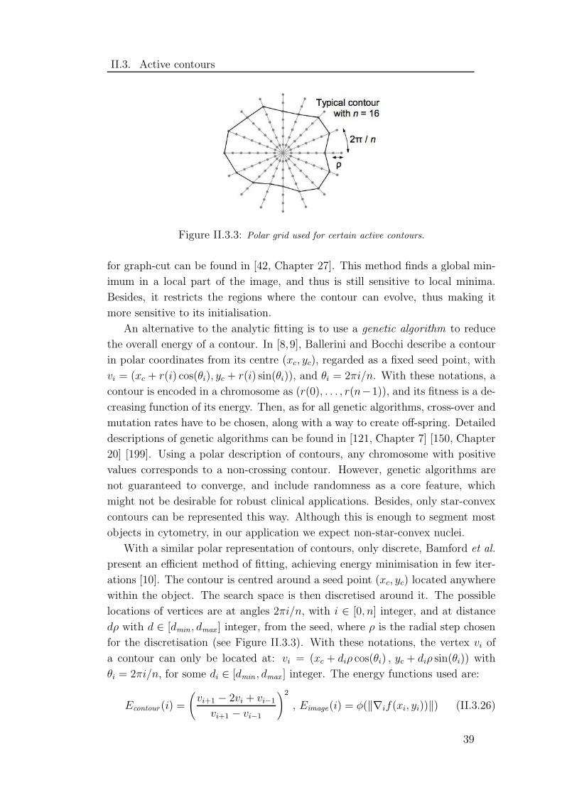
II.3. Active contours
Figure II.3.3: Polar grid used for certain active contours.
for graph-cut can be found in [42, Chapter 27]. This method finds a global min-
imum in a local part of the image, and thus is still sensitive to local minima.
Besides, it restricts the regions where the contour can evolve, thus making it
more sensitive to its initialisation.
An alternative to the analytic fitting is to use a genetic algorithm to reduce
the overall energy of a contour. In [8,9], Ballerini and Bocchi describe a contour
in polar coordinates from its centre (xc, yc), regarded as a fixed seed point, with
vi = (xc + r(i) cos(θi), yc + r(i) sin(θi)), and θi = 2πi/n. With these notations, a
contour is encoded in a chromosome as (r(0), . . . , r(n−1)), and its fitness is a de-
creasing function of its energy. Then, as for all genetic algorithms, cross-over and
mutation rates have to be chosen, along with a way to create off-spring. Detailed
descriptions of genetic algorithms can be found in [121, Chapter 7] [150, Chapter
20] [199]. Using a polar description of contours, any chromosome with positive
values corresponds to a non-crossing contour. However, genetic algorithms are
not guaranteed to converge, and include randomness as a core feature, which
might not be desirable for robust clinical applications. Besides, only star-convex
contours can be represented this way. Although this is enough to segment most
objects in cytometry, in our application we expect non-star-convex nuclei.
With a similar polar representation of contours, only discrete, Bamford et al.
present an efficient method of fitting, achieving energy minimisation in few iter-
ations [10]. The contour is centred around a seed point (xc, yc) located anywhere
within the object. The search space is then discretised around it. The possible
locations of vertices are at angles 2πi/n, with i ∈ [0, n] integer, and at distance
dρ with d ∈ [dmin , dmax ] integer, from the seed, where ρ is the radial step chosen
for the discretisation (see Figure II.3.3). With these notations, the vertex vi of
a contour can only be located at: vi = (xc + diρ cos(θi) , yc + diρ sin(θi)) with
θi = 2πi/n, for some di ∈ [dmin , dmax ] integer. The energy functions used are:
Econtour (i) =
(vi+1 − 2vi + vi−1
vi+1 − vi−1
)2
, Eimage(i) = φ(‖∇if(xi, yi))‖) (II.3.26)
39

II.3. Active contours
where φ is a decreasing function, and ∇i is the gradient of f computed in the
direction θi. The total energy of vertex vi is:
Etotal(i) = λEcontour (i) + (1− λ)Eimage(i) (II.3.27)
where λ is a weighting parameter. Given the seed point, the contour is fully
described by (d0, . . . dn−1). The fitting method consists in choosing the values
di one by one, starting with i = 0, so that the energy is minimum at each
vertex. A dynamic programming technique based on the Viterbi algorithm is
used (see [42, Chapter 16]). The energy of vertex vi is computed for every di and
di+1 (as di−1 is fixed), and the value di chosen is one that minimises:
Si(vi, vi+1) = mindi,di+1
Si−1(vi−1, vi) + Etotal(i) (II.3.28)
A similar method is presented by Chen et al. [33]: they use the same polar
representation, and a similar dynamic programming technique to fit the contour.
The difference lies in the way to close the contour. One contour is fit for every
possible position of v0, and the one with the overall minimum energy is kept. A
similar approach is presented by Xu et al. [196] for lung nodule segmentation,
using expectation-maximisation and dynamic programming, with no mention of
contours. These methods have two significant issues in our context. First, they
can only segment star-convex objects. Second, they are restricted to non-touching
objects.
An improvement for the speed of convergence is presented by Metzler et al.
in [114]. It consists in freezing the edges that are stable, thus reducing the number
of vertices to move in the next iterations. While this method may be useful in
some applications, it will fail when an edge of the contour is stopped at a local
spurious feature of the image. Experiments on our images show that it usually
takes a few iterations for the internal forces to drive that edge out of a spurious
local minima, but with that method it will stay and block its neighbouring edges.
Topology conservation: The following improvements aim at reducing self-
crossing and vertices clustering.
The spreading of internal forces [100] described above smoothes the relative
movements of vertices, thus reducing these risks. Similarly, external forces can be
spread, as done by Ronfard [146]. The image energy computed at vertex vi can
be added to that of its neighbours, with a weight decreasing with their distances.
These methods introduce further parameters though, and only tend to reduce the
risk of self-crossing.
Another way to reduce clustering is to move a vertex vi using only the force
components parallel to nvi[100]. Also, the internal force can be designed to drive
40
II.3. Active contours
vertices towards the centre of gravity of their neighbours. This is achieved in two
dimensions by Pagador et al. [129], and in three-dimensions by Miller et al. [116].
It reduces the possible moves of vertices though, and can be detrimental to the
segmentation of concave objects.
In case vertices clustering does happen, a common way to correct it consists
in merging an edge ei with one of its neighbours when ‖ei‖ is below a threshold,
and creating a new vertex in its centre when ‖ei‖ is above another threshold.
This requires a renumbering of vertices, and is usually performed after a certain
number of iterations, to trade precision against computation time. Choosing the
threshold values is another trade-off: smaller values allow a finer resolution of
the contour, but reduce the effect of internal influences. A less computational
intensive version, presented in [68], consists in doubling or halving the number of
vertices when the mean length of edges reaches out the thresholds.
Self-crossing is intrinsically difficult to avoid. This problem is somehow inher-
ent to contours: influences and movements are computed locally, but self-crossing
is a global issue. The standard approach is to test if any vertex is inside the con-
tour. Detecting if a point lies inside or outside a shape can be done with methods
from computer graphics, such as scan lines. As it is a time consuming operation,
it is usually performed only after a certain number of iterations. Once detected,
it can be difficult to correct. Merging non-neighbouring edges would alter the
contour’s topology. Sudden moves of vertices sharply increase the contour influ-
ences locally, which may cause oscillations or divergence.
A different approach to control the contour shape was introduced by Hamar-
neh et al. [61]. The active contour, named deformable organism, is designed with
an internal structure. Vertices are connected not only by edges, but also by a
skeleton-like structure, made of ‘internal edges’. Their lengths can vary within
given ranges, depending on the variations allowed for the final shape. This method
is a robust way to segment a specific shape that is know in advance, such as organs
or brain structures, while allowing controlled variations. However, it may not be
relevant for the objects usually found in cytometry, where no internal structure
can easily be modeled with edges.
Topological changes: Although the fixed topology of contours is rarely an
issue in cytometry, it is worth mentioning methods that were developed to han-
dle topological changes during the contour fitting. They could be adapted for
the segmentation of clusters, making it more robust with respect to the initial-
isation of contours. Topologically adaptable snakes presented by McInerney and
Terzopoulos [108, 110, 111] evolve over an underlying grid, made of triangles. In
short, after each iteration, the intersections between the edges and the grid define
41
II.3. Active contours
the new contour vertices. This ensures a fairly regular distribution of vertices.
In addition, the topology of the contour can be determined by scanning the grid
cells containing contour edges, and counting the number of edges they contain.
Self-crossing and contour intrusions can be detected efficiently, then contours can
be easily split or merged. Splitting contours, by Lefevre et al. [89], are meant for
tracking purposes, but could be adapted for cluster segmentation. When contour
edges exceed a given length, they are divided into three parts. The contour is
split at these parts if it makes its energy lower. While this may be desirable to
make contours recover from a wrong initialisation, level sets are a more consistent
framework to handle topological changes, as described in the next section.
Multiple contours: Finally, one important improvement for the segmentation
of clustered object is the use of multiple contours that do not inter-penetrate.
In [35], Clocksin introduces a new force. If vertex vi is inside another contour,
a repulsive force is applied to it, directed along −nviand proportional to the
distance of vi within that contour. The weight of this new force is yet another
parameter to tune, and while it is desirable to correct for intruding vertices,
sudden moves of one vertex tend to alter the evolution of the whole contour.
An alternative is to use a force proportional to the area of overlap between the
two contours. The communicating snakes described by Ballerini and Bocchi [9]
are connected with spring-like forces, which keeps them at a fixed distance to
each other. However, this requires many connections between vertices, and new
parameters to tune the importance of these forces. It was introduced to segment
bones, whose number and relative positions are known, but is less relevant in
cytometry.
Prior shape knowledge: Internal influences tend to control the shape locally,
but cannot be used to enforce global shape constraints. When prior knowledge
on the whole shape is available, several methods have been presented to use it
during the contour fitting.
Geometric contours are well suited for prior knowledge, since they are de-
scribed globally as a continuous curve. Prior knowledge on the coefficients de-
scribing the curve can easily be obtained on a set of training shapes. In [164],
Staib and Duncan describe how to include prior distributions in the fitting pro-
cess. Besides, they introduce alternative Fourier parameters that encode the
phase and amplitude of the Fourier components, and are less sensitive to relative
rotations of components. A similar idea is presented by Szekely et al. in [168]: the
distributions of Fourier parameters are stored during a training phase. A mean
contour value is computed, and the deformations modes are extracted by princi-
42

II.3. Active contours
pal component analysis of the covariance matrix of the Fourier parameters. After
the training phase, a contour is fitted to the image, using the main deformation
modes at first, then improving the resolution by introducing more deformations,
in a coarse-to-fine approach. However, computing the deformations requires a
reference in the images, from which the Fourier parameters can be normalised.
This method is well-suited for brain scan images where landmarks can be manu-
ally placed, but is not convenient in our context.
Another approach to include prior knowledge, by Blake and Isard, is detailed
in [15]. It consists in using a template shape Q0, described as a continuous
curve (such as a cubic spline), along with a shape-space, where each vector X
corresponds to a deformation of the template. This assumes that the set of de-
formations needed to obtain any shape from the template are known and simple
(e.g. Euclidian, affine), and applied to the whole shape. These restrictions are
significant in cytometry, where objects can deform locally.
In a recent article [53], Foulonneau et al. compute Legendre moments on train-
ing shapes, and drive the contours towards these values. Legendre moments are
affine-invariant, and thus adapted for the segmentation of objects with known
shapes but varying pose. In our context however, nuclei show large variations of
shapes, which makes the selection of a training set difficult and causes robustness
issues.
A more flexible approach to include prior knowledge was developed by Cootes
[38, 39], as Active Shape Models and Active Appearance Models, respectively
ASM and AAM. These models are trained on a set of objects, initialised near an
object in an image, and adjusted using both the underlying image content and the
training shapes. The training of the two models is based on sets of landmarks po-
sitioned on the segmented objects. The landmarks’ positions and the underlying
textures are encoded as vectors. The distributions of these training vectors are
then modeled with an appropriate parametric model. Using a Gaussian model,
the mean vector and the eigen vectors of the covariance matrix can be computed
easily. A mixture of Gaussian models can also be used, with an Expectation-
Maximisation algorithm, as well as other methods, depending on the types of
deformations to model [40,41]. Once a parametric model is built on the training
set, the active models are initialised near the objects, and fitted iteratively so
that their geometry and the underlying texture falls within the model. While
the general principles of ASM and AAM are similar, their implementations are
different. ASM encode the geometric relations between the vertices and the un-
derlying texture around each vertex, while AAM model the whole texture within
the vertices. As a result, the fitting is performed locally around each vertex for
ASM, and globally on the whole shape for AAM. Compared to active contours,
43

II.3. Active contours
the model of the vertices’ positions plays a similar role as the internal influences,
and the model of the underlying texture, as the external influences. However, in
the active model framework, the two models are encoded globally. As a result,
a shape may have different local geometry and textures, which is not allowed in
most active contours models. These models are well-suited for the segmentation
of objects with consistent geometry and textures, such as faces or brain MRI
images. In our context however, nuclei have very diverse textures and geometry.
No landmark can easily be defined around or inside nuclei, and no corresponding
points can easily be found between two nuclei. Also, clusters of nuclei cause extra
variations of textures and geometry, and would require their own model.
Finally, an extension of geometric active contours consists in embedding the
contour curve as a level set of a higher-dimensional function: this is the basis of
level set segmentation methods, which are detailed in the next section.
44
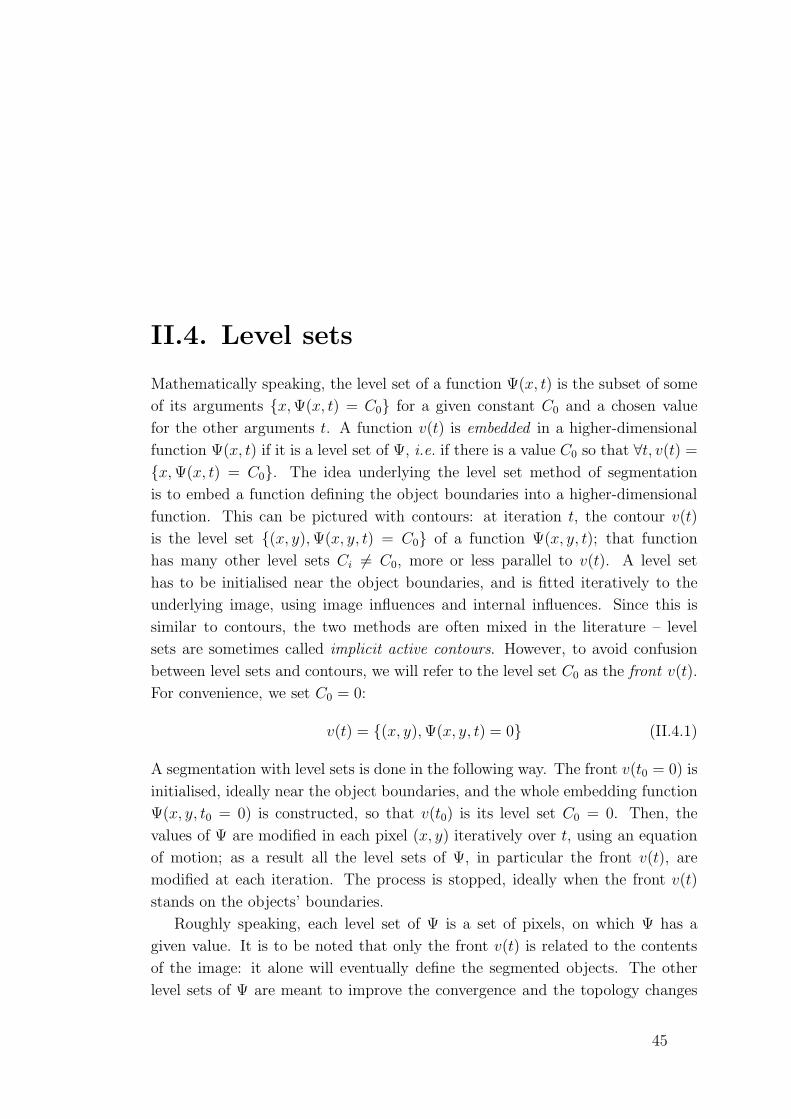
II.4. Level sets
Mathematically speaking, the level set of a function Ψ(x, t) is the subset of some
of its arguments x,Ψ(x, t) = C0 for a given constant C0 and a chosen value
for the other arguments t. A function v(t) is embedded in a higher-dimensional
function Ψ(x, t) if it is a level set of Ψ, i.e. if there is a value C0 so that ∀t, v(t) =
x,Ψ(x, t) = C0. The idea underlying the level set method of segmentation
is to embed a function defining the object boundaries into a higher-dimensional
function. This can be pictured with contours: at iteration t, the contour v(t)
is the level set (x, y),Ψ(x, y, t) = C0 of a function Ψ(x, y, t); that function
has many other level sets Ci 6= C0, more or less parallel to v(t). A level set
has to be initialised near the object boundaries, and is fitted iteratively to the
underlying image, using image influences and internal influences. Since this is
similar to contours, the two methods are often mixed in the literature – level
sets are sometimes called implicit active contours. However, to avoid confusion
between level sets and contours, we will refer to the level set C0 as the front v(t).
For convenience, we set C0 = 0:
v(t) = (x, y),Ψ(x, y, t) = 0 (II.4.1)
A segmentation with level sets is done in the following way. The front v(t0 = 0) is
initialised, ideally near the object boundaries, and the whole embedding function
Ψ(x, y, t0 = 0) is constructed, so that v(t0) is its level set C0 = 0. Then, the
values of Ψ are modified in each pixel (x, y) iteratively over t, using an equation
of motion; as a result all the level sets of Ψ, in particular the front v(t), are
modified at each iteration. The process is stopped, ideally when the front v(t)
stands on the objects’ boundaries.
Roughly speaking, each level set of Ψ is a set of pixels, on which Ψ has a
given value. It is to be noted that only the front v(t) is related to the contents
of the image: it alone will eventually define the segmented objects. The other
level sets of Ψ are meant to improve the convergence and the topology changes
45
II.4. Level sets
Figure II.4.1: Illustration of an embedding function defined as a signed distance. Left: val-
ues of the embedding function Ψ discretised on the image pixels. Right: the same continuous
embedding function Ψ shown in three dimensions. The front v is shown in red.
of the front, but not to segment anything. Thus, the image influences are often
computed for v only, and then extended to the other level sets.
A. Original definitions
Embedding function: The approach we use in this section is based on the
work by Malladi et al. [103]. Once the front v(t0 = 0) is initialised, Ψ is defined
as:
Ψ(x, y, 0) =
−dist(x, y, v) if (x, y) is inside v(0)
0 if (x, y) is on v(0)
dist(x, y, v) if (x, y) is outside v(0)
(II.4.2)
where dist(x, y, v) is the distance between (x, y) and v(0). This definition stands
whether v is discrete (e.g. a set of vertices) or continuous, and whether Ψ is
defined as discrete (over all pixels of the image) or continuous. An illustration
of Ψ is shown in Figure II.4.1. For a description of continuous curves using
Fourier coefficients and cubic splines, we refer the reader to the previous section
on geometric active contours.
Equation of motion: To control the evolution of Ψ over time, its derivatives
are linked by the following equation, called equation of motion:
∂Ψ
∂t(x, y, t) + k(x, y) · (FA + FG(κ)) · ‖∇Ψ(x, y, t)‖ = 0 (II.4.3)
We now detail the terms introduced in the equation of motion.
The partial derivative of Ψ over time is meant to introduce a movement in Ψ.
46

II.4. Level sets
For an iterative solution, it is approximated as:
∂Ψ
∂t(x, y, t) =
Ψ(x, y, t+ ∆t)−Ψ(x, y, t)
∆t(II.4.4)
where ∆t is the time step, a parameter controlling the amount of change allowed
for Ψ between each iteration.
k is the extended speed function. The (non-extended) speed function k is
defined only for the pixels where the front stands, and encodes the image influence
in the equation. However, since the same equation is used for all level sets of Ψ,
k has to be extended to them, thus defining k. The main constraint in designing
k is that it has to be ideally zero at the objects’ boundaries. Supposing the
boundaries are characterised by high gradient, k can be defined as:
k(x, y) =1
1 + |∇f(x, y)| or k(x, y) = e−|∇f(x,y)| (II.4.5)
For more examples of image influences, we refer the reader to the previous section
on active contours. Incidentally, in [103], Malladi et al. define k as above, using
∇Gσ ∗ f(x, y) instead of ∇f(x, y). This simply amounts to smoothing f with a
Gaussian filter of variance σ, which is one of many possible preprocessing. We
consider that any relevant preprocessing was performed on f beforehand. Once
k(x, y) is defined, it can be extended in the following way, called global extension:
k(x, y) = k(x′, y′) (II.4.6)
where (x′, y′) is the point on the front v that is closest to (x, y).
The term FA, standing for ‘advection’, is meant to expand or contract Ψ,
similarly to the pressure force in the balloon model. It can simply be a constant
scalar value c, positive for expansion and negative for contraction1.
The term FG(κ), standing for ‘geometry’, is a scalar value depending on the
curvature κ = κ(x, y, t), defined as:
κ(x, y, t) = div
(∇Ψ(x, y, t)
‖∇Ψ(x, y, t)‖
)(II.4.7)
Using subscript notations for partial derivatives, i.e. Ψx = ∂Ψ∂x
(x, y, t), the curva-
ture is computed as [103]:
κ(x, y, t) = −ΨxxΨ2y − 2ΨxΨyΨxy + ΨyyΨ
2x(
Ψ2x + Ψ2
y
)3/2(II.4.8)
1Expansion of Ψ means that each of its level set expands. Here, it corresponds to a decrease
in the values of Ψ because it is shaped as a pit, not a mountain. Yet, the value added at each
iteration is −c : c ≥ 0 reduces the values of Ψ, thus expanding its level sets.
47

II.4. Level sets
This expression includes a minus sign, simply because the term added to each
iteration is actually −κ. FG is similar to the contour influences presented above,
and is usually meant to penalise high curvature in the level sets. In [26], Caselles
et al. define it as FG(κ) = κ.
Finally, the norm of the gradient of Ψ is:
‖∇Ψ(x, y, t)‖ =(Ψ2
x + Ψ2y
)1/2(II.4.9)
This term corresponds to the amount of change in the values of Ψ around the
point (x, y); in other words, it is higher if level sets are closer to each other around
(x, y).
Using these new notations, Ψ(x, y, t+ ∆t) can be expressed as:
Ψ(x, y, t+ ∆t) = Ψ(x, y, t)−∆t · k · (c + κ) · ‖∇Ψ‖ (II.4.10)
Each point (x, y) is assigned this new value, and may thus be on a different level
set. This way, level sets may expand, shrink, and change topology.
Alternative equation of motion: A different equation of motion, derived
from an energy minimisation view of the level set fitting, is sometimes used [81,94].
It is detailed by Caselles et al. [26,27]. In this model the extended speed function
k(x, y) is called the stopping function g(f(x, y)): it is designed to be zero at the
objects’ boundaries. The equation controlling the evolution of the level set is:
∂Ψ
∂t= ‖∇Ψ‖div
(g(f)
∇Ψ
‖∇Ψ‖
)+ c · g(f) · ‖∇Ψ‖ (II.4.11)
where c is a constant velocity, which in this context should be negative for an ex-
pansion of Ψ. By developing the divergence of a product, and using the definition
of curvature κ = div(
∇Ψ‖∇Ψ‖
), the equation is equivalent to:
∂Ψ
∂t= (c+ κ)‖∇Ψ‖ g(f) + c ∇g(f) · ∇Ψ (II.4.12)
This model is often referred to as geodesic active contour or implicit geodesic ac-
tive contour. In comparison, the model described first in this section is sometimes
called implicit geometric active contour, and with this new notation, the equation
of movement II.4.3 would be written as:
∂Ψ
∂t= g(f) ‖∇Ψ‖div
(∇Ψ
‖∇Ψ‖
)+ c g(f)‖∇Ψ‖ (II.4.13)
A general equation of motion, by Kuhne et al. [82], links these two models:
∂Ψ
∂t= a(f) ‖∇Ψ‖div
(b(f)
∇Ψ
‖∇Ψ‖
)+ c g(f)‖∇Ψ‖ (II.4.14)
where a, b = 1, g. This allows a general analysis of the level set models.
48

II.4. Level sets
Front location: The final step of the iteration is to identify the new location of
the front, which corresponds to solving the equation Ψ(x, y, t+∆t) = 0 for (x, y).
If Ψ is computed discretely over the pixels, one way to solve it is to interpolate
the values linearly between pixels, as in the Algorithm 1 in [103]. In brief, each
pixel (x, y) and its four closer neighbours are considered. Among these five pixels,
if the maximum value of Ψ is positive and the minimum value negative, then the
front should stand between the two pixels where these values are reached. The
pixel closer to the front is found by linear interpolation of these two pixels.
The iteration ends when the new values of Ψ are computed for all pixels,
and the new location of the front is obtained. In the next iteration a new speed
function k will be defined over the new front. The process continues until the
front is stationary.
B. Strengths
With the combined use of internal and image influences, level sets allow the
segmentation of objects with missing boundaries and noise. The general definition
given above can be used for either discrete or continuous level sets, depending on
the resolution and accuracy required for the final segmentation, and the affordable
computation time. With a continuous description, the curvature and normal are
properly defined, thus more robust to the local geometry of the curve.
Another strength of level sets is the front’s ability to change topology in
response to image contents. The front may split, merge, have holes created
or filled, with no extra dedicated step in the algorithm detecting and handling
such changes, as with contours. This may be a useful feature when segmenting
clustered objects.
Also, as the embedding function Ψ is potentially defined over the whole image,
the final segmentation is less dependent on the initialisation of the front.
C. Weaknesses
The high computational time to process level sets is a general weakness. In
particular, the evaluation of the local curvature requires the computation of many
partial first- and second-order derivatives of the embedding function, at every
point and every iteration. Similarly, the extension of the speed function has a
significant cost at each iteration.
Also, the flexible topology may be an issue for some applications: there is no
guarantee that the final segmentation will have a shape or topology similar to the
initial front. Thus, with the original definitions it is actually difficult to include
and keep prior knowledge concerning the global shape of the objects of interest.
49

II.4. Level sets
D. Improvements
Computation time: There are several ways to improve significantly the com-
putation time, in particular the narrow band, the fast marching and the Hermes
methods. In our context, computation time is not a significant issue. We list
these improvements for completeness.
The narrow band method [2,103] is based on the following observation. Only
the front is needed for segmentation, and distant level sets have little influence
on its evolution; yet they increase the computation time. By restricting the em-
bedded function to a few level sets, forming a narrow band around the front, the
final result will be little affected. This require care when evaluating the partial
derivatives at the borders at the band [2]. Since only the level sets within the
band are modified, the front can only be located within in: this may restrict its
topology [103]. A solution is to re-initialise the band regularly, around the new
position of the front. At the latest, it must be re-initialised when the front reaches
the borders.
A further speed improvement of the narrow band technique consists in com-
puting the extended speed function k in the same way as k [103]:
k(x, y) =1
1 + ‖∇f(x, y)‖ (II.4.15)
The fast marching technique is based on a somewhat different vision of level
sets, called front propagation [155]. It may be pictured as a wave v traveling over
the image. In this context, the embedding function of v is T (x, y), whose value
is the time at which v reached the point (x, y). v is still called front, but is now
the outside level set of the embedding function T :
v(t) = (x, y), T (x, y) = t (II.4.16)
It is to be noted that the values of T are not modified once defined: T can only
expand. However, its geometry as a surface may influence the evolution of the
front in a richer way than was possible with active contours. Once stabilised,
the position of the front defines the segmented objects. This time, the equation
describing the evolution of the front boils down to:
‖∇T (x, y)‖ · F (x, y) = 1 (II.4.17)
F is a term controlling the evolution of the propagation. It has to be positive, to
prevent the front from moving back, and large at the objects boundaries, to stop
the front there. An exponential function ensures both constraints:
F (x, y) = exp ‖∇f(x, y)‖2 (II.4.18)
50

II.4. Level sets
The design of F depends on the characteristics of the objects to segment. More
examples are given by Schupp et al. [153]. F may contain terms depending on
the image intensity or gradient, and on the local front geometry. For information,
the curvature of T is defined as [155]:
κ(x, y) =TxxT
2y − 2TxTyTxy + TyyT
2x(
T 2x + T 2
y
)3/2(II.4.19)
This approach of level set runs faster, but restricts the front evolution to one
direction. If the front moves past the object boundaries, it cannot move back
onto them. Viewing the front as a flame expanding and burning the pixels it
passes over, this is summarised as: ‘once a particle is burnt, its stays burnt’.
A combination of narrow band and fast marching, called Hermes, is given by
Paragios and Deriche in [130]. At each iteration only some pixels selected within
a narrow band around the current front are updated.
Finally, another way to improve the computation time is to view the evolution
of the embedding function Ψ as a minimisation problem, which can be solved
efficiently numerically. In [82], Kuhne et al. present a semi-implicit adaptive
operator splitting method to iteratively find the values of Ψ. The equation of
motion is approximated as a linear equation in the form:
Ψ(t+ 1) =1
2
∑
l∈x,y
(I − 2 ∆t Al (Ψ(t)))−1 Ψ(t) (II.4.20)
where Ψ(t) is a vector containing all the values Ψ(x, y, t) at every pixel location,
and Ax(Ψ(t)) and Ay(Ψ(t)) are square matrices containing the terms of the equa-
tion of movement sampled on the pixels. The matrices to inverse are strictly
diagonally dominant tridiagonal, so the system can be solved efficiently. Alter-
natively, in [184], Wang et al. present a minimisation method using Lagrange
multiplier.
Multiple objects: Schupp et al. use fast marching to segment multiple ob-
jects [153]. The propagating fronts have unique labels and are grown in parallel.
When a front reaches a pixel, it assigns it the current iteration time and its
label. If the pixel was already labeled, it stops growing locally. This prevents
inter-penetrating fronts. However, this mechanism relies mainly on a correct
initialisation of all level sets: in particular they are expected to be all at simi-
lar distances from objects boundaries. This makes the segmentation results less
robust to initialisation.
Topology preservation: The original topology of the front can be preserved,
as presented by Han et al. [62]. In addition to narrow band, an underlying grid
51

II.4. Level sets
is used to sample the embedding function Ψ, and may be finer than the pixel
grid. This way, the topology of the front is easier to analyse, and critical points
for its topology (called non-simple points) are not allowed to change values. The
other points are updated normally. The definition of simple points is based on
topological numbers, describing the topology of shapes. This extra step in the
processing requires further computation, and depends on the grid size used. This
introduces yet another parameter to the segmentation method.
Prior knowledge: To include knowledge on shape variations within the seg-
mentation process, Leventon et al. present a method based on statistical distri-
butions of parameters describing the shape [94]. These distributions are stored
as a training set, and used through to a modified equation of motion.
u(t+ 1) = u(t) + λ1F (u(t)) + λ2(u∗(t)− u(t)) (II.4.21)
The term F (u(t)) is from the standard equation of motion u(t + 1) = u(t) +
F (u(t)). The term u∗(t) is the most probable final front given the current front
u(t) and the image: u∗(t) = arg maxu∗ P (u∗|u, f). This probability is decomposed
with Bayes’ rule and evaluated thanks to the probabilities computed during the
training. In the new equation of motion, the parameters λi can be tuned to give
more influence to the image contents or to the training data. An improved version
of this method, using alignment of fronts during the training, was published by
Tsai et al. in [173]. A similar method, using not only prior shapes but also
intensity profiles, is presented by Chen et al. in [32]. As with other methods
based on a training phase, it may be less relevant to cytometry than to other
medical imaging fields, such as image guided surgery [56].
Combination of influences: In the standard implementation of active con-
tours, image influences and contour influences are linearly combined, with tuned
parameters. Conversely, with the standard level sets, the equivalent of the im-
age influence, k, and that of the contour influence, FG(κ), are multiplied. This
removes the need for tuning before segmentation. However, at least one of the
terms has to be zero for the level set to stop moving. Since the curvature is usu-
ally high, it is the image speed that stops the iterations. Whereas in the contour
models, the influences may balance each other, even when none is zero. In case
this feature of level sets is undesirable, linear combinations of influences can be
used instead, as in the RAGS model presented by Xie and Mirmehdi in [192].
52

II.5. Other methods
In this final part, we mention other segmentation methods that have been widely
used in various fields of computer vision, but are not as popular in published
cytometry than the ones cited before.
II.5.1 Region growing
Region growing consists in grouping neighbouring pixels based on their similar-
ity [48]. A region is grown from a seed pixel, and the pixels at the border of the
region are gradually added if a similarity measure between them and the region
is within a given range of values. The process stops when no more pixels are
added. Similarity can be based on a statistical model of the object’s histogram.
The model may also be dynamically updated during the region-growing process.
The main strengths of region growing are its fast execution, its ease of imple-
mentation, and its flexibility. The models used are not necessarily Gaussian, as
any measure of similarity can be used to compare pixels. Also, the models can
be updated at runtime.
However, the resulting segmented regions usually have irregular borders and
holes. Region growing is intrinsically a bottom-up process, and is not meant to
include prior knowledge on global shapes. Besides, as it only segments homoge-
nous regions, it often results in oversegmentation. Also, as it may be difficult
to design a similarity criterion that excludes noise, region growing is potentially
very sensitive to noise. Finally, a dynamic adaptation of the model makes the
results highly dependent on the location of the seed.
A first improvement, by Sclaroff and Liu, aimed at incorporating prior shape
knowledge consists in running two consecutive region growings [154]. The first
time, the image is oversegmented in small homogenous regions. The second it-
eration actually merges them: regions are merged if their overall shape fits a
deformable template, in a way similar to energy-based active contours. Inciden-
53

II.5. Other methods
tally this second step is often used after a watershed transform. It requires a
model of possible shapes adapted to the oversegmentation results: this is not
practical for our application.
Another improvement concerns the robustness and automation of the region
growing, as presented by Pohle and Toennies [134, 135] for organ segmentation.
From a seed selected manually, a first region growing is performed, using dy-
namic adaptation of the similarity model. In more details, the object’s intensity
histogram is modeled as a Gaussian, and the mean and variance are evaluated
every time the segmented region doubles in size. A tabulated correction factor is
used to compensate for the under-estimated standard deviation during the grow-
ing. Once the growing is over, the final values of the mean and deviation are
stored. A second run of region growing is performed, from the same seed, using
these stored values as a fixed model all along the process. The segmented regions
are then merged using their similarities and a shape factor. Apart from the man-
ual seed location, which has to be near the objects’ centres, this method may be
automated. It is very specific to their application though. In our context, seed
location cannot be manual, and single Gaussian models are not adapted to the
variety of textures found in our context.
II.5.2 Neural networks
Neural networks represent a large field of research and applications in computer
science, and presenting them is beyond the scope of this chapter. For detailed
introductions to neural networks, we refer the reader to [121, Chapter 6], [150,
Chapter 19]. Neural networks are reputed for their classification properties. How-
ever, classification often require segmentation results as an input, as for exam-
ple [127], and is not the focus of our work.
A comprehensive review of the use of neural networks for image processing
was recently published by Egmont-Petersen et al. [49]. Their section on image
segmentation lists the possible networks that can be used, with many references,
along with their limitations.
In [137], Poli and Valli present a segmentation method based on Hopfield net-
works, applied to images of brain and organs. A network is build with several
two-dimensional layers of neurons, each layer corresponding to a label. Each pixel
is assigned to one neuron in each layer. The energy of the network is made of
two parts: a sensitivity energy, which is meant to be minimum at the boundaries,
and a robustness energy, lower for large connected regions. The network is ini-
tialised by a first probabilistic segmentation based on morphological thresholding,
and then evolved so as to minimise its energy. The use of energies makes this
54

II.5. Other methods
method somehow similar to active contours. However, the robustness energy is
not enough to include prior knowledge on shape, which is a general weakness of
neural networks for segmentation. Also, such a network is sensitive to the actual
location of objects on an image. In our context nuclei can be present literally
anywhere on images.
A different use of neural networks in presented by Ossen et al. in [127]. Their
idea is to add a classifier step after the segmentation, and use the results of
the classification as new parameters for a further segmentation. They use back-
propagation feed-forward neural network as a classifier, and texture properties of
the segmented objects to compute a posteriori probabilities. Useful as it is, this
step is not linked to segmentation, but to object recognition, beyond the scope
of our work.
Finally, Shareef et al. use oscillatory networks for segmentation of brain im-
ages [158]. It is meant to group pixels based on their similarities. This method
is also specific to the imaging protocols used, namely MRI and CT, and is not
adapted to fluorescent microscopy.
II.5.3 Region competition
We present region competition, by Zhu and Yuille [203,204], for completeness. It
is based on principles underlying active contours, region growing and probabilis-
tic segmentation. It requires prior models of the object intensity distributions.
A region of the image is called homogenous if its intensity values correspond to
one predefined model. As it is unlikely that a region fits a model perfectly, the
homogeneity of a region is measured as its probability of corresponding to a given
model.
Region competition is an iterative segmentation based on energy minimisa-
tion. A region, characterised by a specific parametric model (e.g. of its histogram)
is grown from a seed. Pixels are added to a nearby region based on its similar-
ity with the region’s model, using a probabilistic framework. Since the models’
parameters and the region’s contents are co-dependent, but unknown to start
with, they are evaluated iteratively, with a greedy method. After the first region-
growing, the models’ parameters are re-evaluated. These new parameters are then
fixed, and the objects’ boundaries are modified using two forces. A smoothing
force, which is high where the boundary has a high curvature, will straighten the
boundary, while a statistics force, which is weak when the region has a high ho-
mogeneity, will compress the region. If the regions do not cover the whole image,
a new seed is selected inside uncovered parts, and a new run of the greedy region
growing method is performed. Once all the image is segmented, the next step of
55

II.5. Other methods
Figure II.5.1: Image segmented with dynamic graph-cut. Left: original image. Right: results
of the dynamic graph-cut. The pixel brightness is proportional to their likelihood of belonging to
a nucleus. Although the boundaries are generally correct, the results inside the nuclei are noisy.
the algorithm merges neighbouring regions if that reduces the overall energy over
the image. If no regions were merged, the segmentation is over; otherwise, after
merging, a new run of the greedy method is performed.
This method is reported to be robust to the original selection of seeds [203,
204]. A feature of the region merging process can automatically rule out irrele-
vant regions – i.e. regions that are either not part of an object or which did not
pick the correct model.
By combining active contours and region growing, this method also keeps their
drawbacks. In particular, it requires the tuning of many parameters for different
steps of the segmentation. It also requires that each region has a distinct para-
metric model, which also needs to be learnt from the image. This is not adapted
for our application, where all nuclei in a given image tend to have very similar
histograms.
II.5.4 Graph cut
Graph cut refers to a wide family of algorithms, meant to separate weighted
graphs in subparts [42]. For image segmentation, they are usually performed on
Markov Random Fields [13, 17]. As these two topics are beyond the scope of
our review, we only summarise them. Markov Random Fields assign labels to
pixels and underlying connections between pixels. In a probabilistic framework,
the label assigned to each pixel depends on its intensity, and also on the labels
of the connected pixels. By assigning a penalty or a cost to each pixel and each
pairs of pixels, a weighted graph is built on the whole image. The subgraphs
that can be isolated by separating pairs at a minimal cost, in other words by
performing a min-cut on the graph, can be interpreted as different segmented
regions. Unlike active contours, this method achieves a global minimisation of
the functions used to define the penalties. However, the definition of the penalties
56

II.5. Other methods
is mainly restricted to absolute pixel intensities and connected pixel values [79].
Also, in a way similar to level sets, it is difficult to encode shape or topology
constraints on the segmented regions.
Recent improvements of graph-cuts include the addition of shape priors in
the graph weights [84]. As explained above, prior knowledge on shape is difficult
to obtain reliably in our context. Another extension of graph-cut consists in
assigning a confidence value instead of a label to pixels [77]. An example of this
method is shown in Figure II.5.1. This method, however, cannot be used as a
standalone for our needs, but only as a pre-processing. The image still needs
to be post-processed to isolate the distinct nuclei, and touching nuclei can be
difficult to separate. This method is more adapted to images showing a single
object with a regular texture.
57
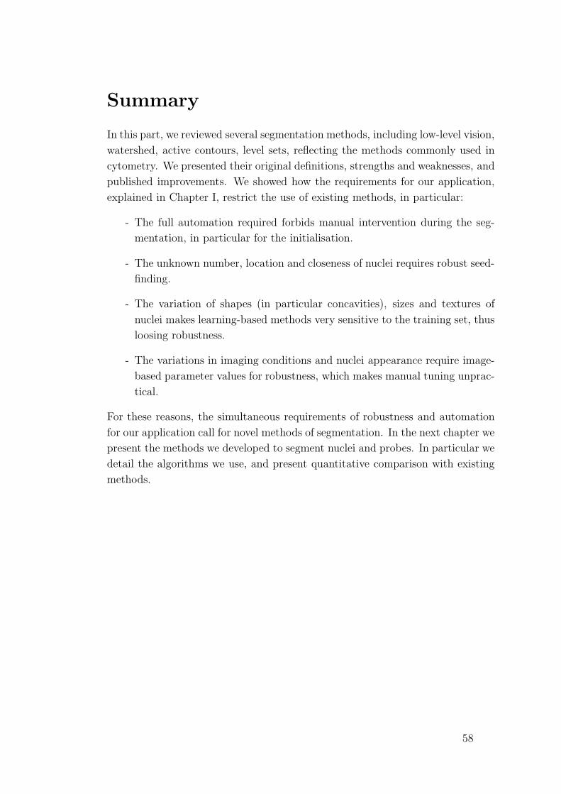
Summary
In this part, we reviewed several segmentation methods, including low-level vision,
watershed, active contours, level sets, reflecting the methods commonly used in
cytometry. We presented their original definitions, strengths and weaknesses, and
published improvements. We showed how the requirements for our application,
explained in Chapter I, restrict the use of existing methods, in particular:
- The full automation required forbids manual intervention during the seg-
mentation, in particular for the initialisation.
- The unknown number, location and closeness of nuclei requires robust seed-
finding.
- The variation of shapes (in particular concavities), sizes and textures of
nuclei makes learning-based methods very sensitive to the training set, thus
loosing robustness.
- The variations in imaging conditions and nuclei appearance require image-
based parameter values for robustness, which makes manual tuning unprac-
tical.
For these reasons, the simultaneous requirements of robustness and automation
for our application call for novel methods of segmentation. In the next chapter we
present the methods we developed to segment nuclei and probes. In particular we
detail the algorithms we use, and present quantitative comparison with existing
methods.
58

Chapter III
Evaluating the Telomere
Intensity in Leucocyte Nuclei
from Different Individuals
59
In this chapter we present our novel segmentation methods. We start with the
segmentation of nuclei, detailing our novel model for the image and our adap-
tation of the Expectation-Maximisation (EM) algorithm to adjust our model’s
parameters to an image. We then present our segmentation method for telomeric
probes, based on a new dome-detection algorithm. We compare both our meth-
ods with existing methods, and discuss the strengths of our approaches. Finally,
we present the results we obtained with our methods on the data set used for the
pilot study.
Figure III.0.2: Left column: Images showing leucocyte nuclei (in blue), containing probes
attached to the telomeres (in green). Right column: nuclei and probes segmented with our
methods.
60

III.1. Segmentation of nuclei
To segment the nuclei under the requirements of robustness and significant varia-
tions in the image properties described in Chapter I, we developed a new method
of segmentation. It is a three-step method, outlined below. Its details are pro-
vided in this section, and a summarising illustration is shown as Figure III.1.5
page 72.
Step 1: Find the image regions containing nuclei. The method starts by
modeling the image’s histogram with a novel model accounting for each part
of the image accurately. This model is fitted to the histogram automatically,
with an Expectation-Maximisation algorithm that we adapted for histogram
matching. Once fitted, the model is used to find a global threshold value
removing most of the background. Each of the segmented regions contains
nuclei and still some background.
Step 2: Delineate the nuclei. Each region segmented in step 1 is processed
separately with the same method. The histogram model is fitted to the
region’s histogram with the adapted EM algorithm, and is used to define
a local threshold. The thresholded components do not contain background
any more, but may contain touching nuclei. They will be used as masks for
the final operation.
Step 3: Separate the touching nuclei. To detect and separate touching nu-
clei, the model fitted to the region’s histogram is used to define a higher
threshold. Each isolated component corresponds to the inside of a single
nucleus, and is marked as a seed. A fast region growing based on distance
transform within the masks found previously is performed on the seeds to
obtain the final segmentation of nuclei.
Before explaining our segmentation method, we detail first its core features,
namely our histogram model and our adapted EM algorithm. We then explain
61

III.1. Segmentation of nuclei
Figure III.1.1: Background illumination. Top left: image with segmented nucleus, illuminated
and non-illuminated background. Bottom left: intensity values along the horizontal line across
the image. Right: Histograms of the three segmented regions (The vertical scale is bilinear, as
reflected by the values on the side).
our complete segmentation method, in particular how we use our model to derive
the threshold values needed in each of the steps described above. Finally we
present and discuss the results obtained with our method, compared with other
methods we implemented.
III.1.1 Model of the histogram of an image
As explained in Chapter I, the nuclei have been treated with fluorescent marker
DAPI, and when illuminated with light at their exciting wavelength, they diffuse
light all around them. The light emitted from the nuclei upwards, towards the
microscope lenses, is not the only light collected on the CCD camera though. Part
of the light emitted sideways is deflected by the surrounding materials, and part of
that deflected light will be collected by lenses and the camera. The resulting image
shows a dim enlightenment of the background regions surrounding nuclei. This
effect is hardly noticeable by eye, but alters significantly the background intensity
values, increasing them up to three-fold. Taking this effect into account is critical
to the correct segmentation of the nuclei, but has not yet been addressed directly,
to the best of our knowledge. We introduce the term illuminated background to
62

III.1. Segmentation of nuclei
denote the affected background regions surrounding the nuclei, as opposed to the
non-illuminated background. Figure III.1.1 page 62 shows the three regions of
a typical image, a profile of intensities across them, and their histograms. The
profile and the histograms show the raise of intensity values in the illuminated
background, marked in red.
The extent of the non-illuminated background depends on several unknown
or inaccessible parameters, such as the shapes, sizes, concentrations of the nuclei,
the quantity of markers they contain, the intensities of light they received or
the exposure time. Therefore it cannot be determined directly from an image
before segmentation. However, the histograms of the nuclei, the non-illuminated
and illuminated backgrounds can be extracted from the histogram of the whole
image, in a way described in Section III.1.2. Once extracted, these histograms
can be used to segment the nuclei, as explained in Section III.1.3.
As illustrated in Figure III.1.1, an image’s histogram consists of three slightly
overlapping parts: a sharp peak in the lowest values, a sharply decreasing curve
in the medium values, and a plateau with any number of domes and valleys in the
highest values. They correspond respectively to the non-illuminated background
(NIB), illuminated background (IB), and nuclei (N). In this section, we present
the parametric functions we use to model each part, with particular emphasis on
our new model for the illuminated background. Let h(I) be an image histogram,
consisting of parts NIB, IB and N, which we aim to model with hmodel (I).
Non-Illuminated Background. To model the NIB, we assume that it con-
tains Ab pixels, has a mean value Ib, and is affected by Gaussian noise of standard
deviation σb. Using a Gaussian model is supported by observations of images con-
taining no nuclei. The NIB is modeled with:
NIB(I) =Ab√2πσb
exp
(−(I − Ib)2
2σ2b
). (III.1.1)
Nuclei. The part of the histogram corresponding to the highest intensities,
N, reflects the textures of the nuclei, which show high variability within and
across images. In particular, variations affect the range of intensity values, the
shape of the histogram and its number of peaks, as illustrated in Chapter I.
Also, saturation can occur at high intensities, depending on the procedure and
hardware used for imaging. To overcome these problems, we model the histogram
of the nuclei with a sum of Gaussians: this is both robust and flexible enough
for our needs. Since we do not know in advance how many nuclei are on an
image, nor how many Gaussians are needed for each texture, we introduce a new
parameter, n, the number of Gaussians modeling the nuclei’s histogram. Each of
63

III.1. Segmentation of nuclei
Figure III.1.2: Illustration of our model. Left: model of a circular nucleus. Center: model of
the intensity values in the illuminated background, I (r), defined in Equation (III.1.3). Right:
model of the histogram of the illuminated background, IB(I ), defined in Equation (III.1.12).
these Gaussians i will model Ai pixels, with mean Ii and deviation σi:
Ni(I) =Ai√2πσi
exp
(−(I − Ii)2
2σ2i
), 1 ≤ i ≤ n . (III.1.2)
Illuminated Background. Our model of the illuminated background’s his-
togram is based on a model of the physics that generates it. We model the
light diffused outside a nucleus as a function of the distance to that nucleus, and
integrate it all around the nucleus. We then use this model to measure the back-
ground area having a given intensity. Finally we apply it to integer intensities
to obtain a model of the histogram of the illuminated background. Given that
our model will only be used for intensity values I above the mean background
value Ib with I − Ib ≫ 1, we develop expressions to the first order in 1I−Ib
when
appropriate.
We consider a circular nucleus, as illustrated in the left of Figure III.1.2, but
will then make our model independent from the nucleus’ shape. Let I0 be the
intensity at the border of the nucleus, at distance R0 from its center, and Ib be
the average intensity of non-illuminated background. We model the intensity in
the illuminated background, along a line normal to the nucleus, with a decreasing
exponential (see middle of Figure III.1.2):
I(r) = Ib + (I0 − Ib) · exp
(−r − R0
ρ
), for r ≥ R0 . (III.1.3)
The parameter ρ controls the slope of the intensity’s decay: it corresponds to
the distance outside the nucleus at which the intensity has decreased by 1e≈
37%. Our model, however, cannot be fitted directly to an image for segmentation
purposes as it requires a prior segmentation of the nuclei. Nevertheless, it can
be used to derive a model of the histogram of the illuminated background. This
64

III.1. Segmentation of nuclei
latter model will be easier to adjust to the image histogram, as detailed in the
next section. We now explain how to derive that model.
The expression of I(r) in Equation (III.1.3) can be inverted to define r(I):
r(I) = R0 − ρ · lnI − IbI0 − Ib
(III.1.4)
Using Equation (III.1.4), the number of points dn(r) = 2π r dr at distance r from
the nucleus can be expressed as a function of the intensity:
dn(I) = 2π(R0 − ρ · ln
I − IbI0 − Ib
)· ρ · −dI
I − Ib(III.1.5)
Introducing the new parameters α = ρR0
and A = πR20, dn(I) can be written as:
dn(I) = 2Aα(1− α ln
I − IbI0 − Ib
) −dII − Ib
. (III.1.6)
The expression of dn(I) is now independent of the actual shape of the nucleus. It
only depends on its area A and the dimensionless parameter α, which controls the
extent of the illumination relative to the size of the nucleus. By integrating dn(I)
between I and I + 1, we obtain by definition the histogram of the illuminated
background. Since dn(I) is a decreasing function of I, its has to be integrated
from I + 1 to I:
IB(I) =∫ I
I+1dn(I ′) = 2 A α
∫ I+1
I
dI ′
I ′ − Ib︸ ︷︷ ︸a
−α∫ I+1
Iln
(I ′ − IbI0 − Ib
)dI ′
I ′ − Ib︸ ︷︷ ︸b
(III.1.7)
The two terms a and b of Equation (III.1.7) can be integrated separately and
developed in the first order with respect to 1I−I0
. The first term is:
a = [ln(I ′ − I0)]I+1I = ln
(1 +
1
I − I0
)=
1
I − I0+ o
(1
I − I0
)(III.1.8)
The second term can be integrated with the change of variables X = I′−Ib
I0−Ib:
b =∫ I+1−Ib
I0−Ib
I−IbI0−Ib
lnX
XdX =
[1
2ln2X
] I+1−IbI0−Ib
I−IbI0−Ib
(III.1.9)
Using the identity ln2 x− ln2 y = ln(x y) · ln xy, b can be factorised and developed
with respect to 1I−Ib
:
b = ln(1 +
1
I − Ib
)·(ln(I − IbI0 − Ib
)+
1
2ln(1 +
1
I − Ib
))
=(
1
I − Ib+ o
(1
I − Ib
))·(ln(I − IbI0 − Ib
)+ o(1)
)
b =1
I − Ib· ln
(I − IbI0 − Ib
)+ o
(1
I − Ib
)(III.1.10)
65

III.1. Segmentation of nuclei
Using Equations (III.1.8) and (III.1.10) in Equation (III.1.7), we get:
IB(I) =2 A α
I − Ib
(1 + α ln
(I0 − IbI − Ib
))+ o
(1
I − Ib
)
IB(I) =2 A α2
I − Ibln(I0 − IbI − Ib
)+O
(1
I − Ib
)(III.1.11)
Keeping only the first-order term in Equation III.1.11 leads to the definition of
our model of the illuminated background’s histogram:
IB(I) =2 A α2
I − Ibln(I0 − IbI − Ib
). (III.1.12)
This function is illustrated in the right-hand side of Figure III.1.2. The two
parameters A and α correspond respectively to the area of the nucleus creating
the illumination, and to the spatial decay of the illumination. The two parameters
Ib and I0 corresponds respectively to the mean intensity of the non-illuminated
background and to the intensity at the border of the nucleus causing the illumi-
nation.
To link this model with that of the nuclei, we assume that each Gaussian
modeling the nuclei creates part of the illumination. Let IB i(I) describe the
background illuminated by Ni(I). Three of its four parameters are constrained
by the rest of the model: the area causing the illumination A = Ai, the mean
intensity Ib of the non-illuminated background, and the intensity at the border
of the nucleus. We set the value of this latter parameter to I0 = Ii − 2σi: it
corresponds to the darker 5% of the nucleus’ pixels, which we consider to be on
the boundary. This way, the functions modeling the illuminated background are:
IB i(I) =2 Ai α
2i
I − Ibln(Ii − 2σi − Ib
I − Ib
). (III.1.13)
Let Φn be the set of all the functions used, which are defined in Equations (III.1.1),
(III.1.2) and (III.1.13). The model of the histogram is:
hmodel (I) =∑
g∈Φn
g(I) , where Φn = NIB ∪⋃
1≤i≤n
IB i, Ni . (III.1.14)
It depends on the 4(n+ 1) parameters n,Ab, Ib, σb, Ai, Ii, σi, αi1≤i≤n. They are
adjusted to an image histogram using our adapted Expectation-Maximisation
algorithm, as detailed in the next section.
III.1.2 Expectation-Maximisation algorithm for
histogram modeling
The term Expectation-Maximisation (EM) refers to a class of algorithms that iter-
atively fit a parametric model to incomplete data [172]. The missing data may be
66

III.1. Segmentation of nuclei
either missing points in a series (e.g. missing pixels in an image, or missing frames
in a video), or missing dimensions: a typical example is the missing labeling of
pixels in a non-segmented image. Given the parameters of the model of the com-
plete data, the missing points or dimensions may be inferred from the available
data. Reciprocally, supposing the available data was complete, the parameters
of the model could be computed properly. The problem of fitting a parametric
model to incomplete data is that neither the parameters nor the complete data
are available in the first place.
The idea underlying an EM algorithm is that the parameters can be estimated
given an estimation of the complete data, resulting in a new model. Then, the
missing data can be re-estimated based on the latest model. Iterating these steps
may result in a convergence of the model to the existing data, and at the same
time in a stable estimation of the missing data. Oscillations or divergence may
occur, in which case the EM algorithm should be initialised differently.
Formally, let f be the available data, g the missing data, and D = (f, g) the
complete data. Let Φ(pi) be a parametric model of D, depending on the set of
parameters pi. The two versions of EM algorithms fitting Φ to D are presented
in Algorithm 1.
Algorithm 1 General Expectation-Maximisation algorithm: Two versions
Version 1: Estimating the parameters first
1: Initial E-step: estimate pi given f
2: repeat
3: M-step: estimate g given f and Φ(pi)4: E-step: estimate pi given D = (f, g)
5: until convergence
Version 2: Estimating the missing data first
1: Initial M-step: estimate g given f
2: repeat
3: E-step: estimate pi given D = (f, g)
4: M-step: estimate g given f and Φ(pi)5: until convergence
The criterion for convergence depends on the model used and the results ex-
pected. For example, the iterations can be stopped as soon as the error between Φ
and D (defined accordingly) stops decreasing, or reaches a given threshold value.
Alternatively the iterations may be performed a fixed number of times, and the
final model Φ is one that had a minimal error.
The terms Expectation and Maximisation refer to the versions of such al-
gorithms that use the statistical Expectation to estimate the parameters of the
67

III.1. Segmentation of nuclei
Figure III.1.3: Illustration of the proportions. At intensity I0, the function IB accounts for
20% of the modeled value of the histogram, and the function N for 80%.
model in the E-step, and that estimate the missing data in the M-step by maximis-
ing the likelihood that the current model fits the complete data. Such algorithms
are commonly used in Computer Vision to fit a mixture of Gaussian models to
data with missing labels. In a probabilistic framework, such algorithms also in-
clude constraints on the model to ensure that the probabilities of a model or at a
point add up to 1. Such constraints, however, come from the use of probabilities,
not the use of an EM algorithm.
To explain how we fit the models defined in the previous section to an image
histogram with an EM algorithm, we first introduce the notion of proportions.
Let h(I) be an image histogram, consisting of parts NIB, IB and N, which we aim
to model with hmodel (I). Each intensity I in the histogram contains a proportion
of pixels modeled by each function of our model (see Figure III.1.3). We define
this proportion as:
pf (I) =f(I)
∑g∈Φn
g(I), ∀f ∈ Φn . (III.1.15)
Knowing these proportions is enough to define the successive thresholds needed
for our nucleic segmentation, as detailed at the end of this section, and is there-
fore our goal. Should the model’s parameters be known, the proportions can be
computed using Equations (III.1.1), (III.1.2), (III.1.13) and (III.1.15). Recipro-
cally, given all the proportions pf(I), ∀I, ∀f ∈ Φn, the model’s parameters can
be computed as described below. However, neither the parameters nor the pro-
portions are available in the first place. As explained above, this type of problem
can be solved by Expectation-Maximisation [172].
The algorithm we use, presented as Algorithm 2, is adapted to histograms:
the steps are the same as in Algorithm 1 Version 1, only the equations used are
specific. As explained in the previous section, the number of Gaussian n needed
to model the nuclei’s textures is unknown. To find the model which best fits an
image’s histogram, we iterate the EM algorithm with increasing values of n, and
keep the model with the lowest error.
68

III.1. Segmentation of nuclei
Algorithm 2 Expectation-Maximisation algorithm for histogram modeling
1: for n = 1 to 5 do
2: Initial E-step: set the initial proportions as listed in Table III.1.1.
3: for 100 times do
4: M-step: compute the parameters with Equations (III.1.16) and (III.1.22).
5: E-step: update the proportions with Equations (III.1.1), (III.1.2),
(III.1.13), (III.1.15).
6: Evaluation: measure the error between the model and the histogram
with Equation (III.1.23). Store the model if the error is the lowest.
7: end for
8: end for
9: return the model with the lowest error.
Table III.1.1: Initial values of the proportions used for the EM algorithm.
Intensity 0 . . . 1n+2
Imax1
n+2Imax . . .
2n+2
Imaxj+1n+2
Imax . . .j+2n+2
Imax , 1 ≤ j ≤ n
pNIB(I) 0.9 0.1 0
pIBi(I) 0.1/n 0.9/n 0.1/n
pNi(I) 0 0 0.9 if i = j , 0 else
Initial E-step: Given a value of n, the initialisation step is performed as fol-
lows. Intuitively, most of the dark pixels are modeled by NIB , most of the bright
pixels by either one of the Ni, and most of the remaining pixels by the IB i (see
Figure III.1.1). The range [0, Imax ] of the histogram is divided in n+ 2 segments,
and each proportion is initialised by a fixed value on each segment. The actual
values we use are listed in Table III.1.1.
M-step: We now detail how to compute the parameters of our model given the
histogram h(I) and all the proportions pf (I). Regarding the Gaussian functions
NIB and Ni, the total, mean and deviation of a weighted histogram are evaluated
as [161]:
Ai =∑
I
pNi(I) h(I) ; Ii =
∑
I
pNi(I) h(I) I ; σ2
i =∑
I
pNi(I) h(I) (I − Ii)2
(III.1.16)
For the remaining functions IBi , the only parameter to compute is αi. Using
the notation of Equation III.1.6, the sum of histogram values of the illuminated
background between any two values I1 and I2 is:
I2∑
I=I1
IB(I) =∫ I2+1
I1dn(I) (III.1.17)
69

III.1. Segmentation of nuclei
However, dn(I) is only defined and positive between Ib and I0, and is not summable
near Ib. Let Iε = Ib + ε (I0 − Ib), where ε ∈ (0, 1):
I0−1∑
I=Iε
IB(I) =∫ I0
Iε
dn(I) (III.1.18)
Developing to first order terms, we get:
I0−1∑
I=Iε
IB(I) = −2Aα2∫ I0
Iε
ln(I − IbI0 − Ib
)dI
I0 − Ib(III.1.19)
Since IB(I0) = 0, the sum can be extended to I0, while the integral can be
computed with a change of variable:
I0∑
I=Iε
IB(I) = Aα2 ln2 ε (III.1.20)
This gives the expression of α as a function of the model values:
α =1
| ln ε|
√√√√ 1
A
I0∑
Iε
IB(I) (III.1.21)
To evaluate αi from a labeled histogram, we replace IB(I) in Equation (III.1.21)
with its evaluation pIB ih(I) :
αi =1
| ln ǫ|
√√√√√ 1
Ai
Ii−2σi∑
I=Iǫ
pIB ih(I) (III.1.22)
where Iε = Ib + ε (Ii − 2σi − Ib). In our application we use ε = 0.1.
E-step: Given a parametric model Φn = NIB∪⋃1≤i≤nIB i, Ni, the propor-
tions can be computed directly from their definitions in Equation (III.1.15).
Evaluation: The error we use to evaluate a given set of parameters has to
reflect how each part of the model fits the histogram, as equally as possible. The
main issue is that the histogram values corresponding to the Ni components are
about 20 times lower than that of the NIB . However, it is important that both
parts are correctly modeled at the same time. To overcome this issue, we use the
error measure of the χ2 test:
error =∑
I
(1− hmodel (I)
h(I)
)2
(III.1.23)
Using Algorithm 2, the parameters of our model for the image histogram can be
adjusted automatically. In the next section we explain how to use a fitted model
to segment the nuclei, by defining global and local thresholds.
70

III.1. Segmentation of nuclei
III.1.3 Complete segmentation of the nuclei
The complete segmentation of the nuclei is performed in three steps, as illustrated
on Figure (III.1.5). First, we use the algorithm above to adjust our parametric
model to the image histogram. Once the model is fitted to the histogram, let:
θglobal = max I : ∀i , min(pNIB(I), pIBi(I)) ≥ pNi
(I) . (III.1.24)
Below this value, all intensities contain more points from NIB or IB i than from
the corresponding Ni – and it is the highest such value. This is the global thresh-
old we use to discard the non-illuminated and part of the illuminated background.
Then, in each of the segmented regions, we apply the same algorithm to find a
model of the histogram (without the NIB function this time). In a similar way,
we find the highest intensity containing more points from all IB i than from all
Ni, and use it as a local threshold θlocal :
θlocal = max
I :
n∑
i=1
pIBi(I) ≥
n∑
i=1
pNi(I)
. (III.1.25)
The definition of the global threshold is more strict than that of the local
threshold, for the following reason. In the global histogram it is more difficult
to draw a limit between dark nuclei and bright illuminated background. Since
the image intensity tend to vary across an image, brighter parts of the image
containing brighter nuclei will also have brighter illuminated background. Using
the sum of the IB and N functions in the global model would penalise darker
nuclei in darker parts of the image.
The newly segmented components do not contain background any more; how-
ever, they might contain more than one nucleus. This is often resolved by studying
the concavities of the nuclei’s outlines [85], but cannot be applied to uncultured
nuclei. We consider the texture instead, which is already modeled by the Ni,
and assume that there is more than one distinguishable nucleus if there is a dark
path in the region separating two bright components. The threshold we use for
this test, called inner threshold θinner , is the lowest of the Ii. The connected
components above θinner are considered as seeds: each one marks a unique nu-
cleus. We then extend the seeds into the regions above θlocal using a fast distance
transform [51], reproduced in Appendix A page 128, to obtain the separated nu-
clei. Figure (III.1.5) shows the three steps of the segmentation, with the models
adjusted to the histograms. Examples of segmented images are shown in Fig-
ure III.0.2 page 60.
71

III.1. Segmentation of nuclei
Figure III.1.4: Global and local thresholds obtained from a fitted model.
Figure III.1.5: The stages of nucleic segmentation. Top row, left to right: original image;
its histogram with our adjusted model superimposed; the components of our model, used to find
a global threshold removing most of the background; the segmented image, with two segmented
regions containing nuclei but also some background. Middle row: one of these regions; its
histogram and our adjusted model; the components of our model, used to find a local threshold,
removing the remaining background; the segmented region, with no more background, but where
the two nuclei are still undistinguished: it will be used as a mask for the final step of the
segmentation. Bottom row: the segmented region; the components of our model, used to find
an inner threshold, removing the darkest parts of the nuclei; the segmented nuclei, isolated but
with parts missing: they are used as seeds, and grown with a fast distance transform within the
mask defined above; the resulting segmentation of the region, with two separated nuclei and no
background.
72

III.1. Segmentation of nuclei
III.1.4 Results and discussion
We present the quantitative results obtained using our two methods of segmen-
tation. Our data set contains 2,166 images, showing overall about 14,000 nuclei
and 315,000 probes. For comparison, we also implemented a watershed-based
method for nucleic segmentation, detailed in [104].
Nucleic Segmentation. We implemented our method as described above, on
an iMac with a 1.8GHz PowerPC G5 with 1Gb of RAM. The EM algorithm is
used with up to 5 histogram components, fitted during 100 iterations, with initial
values as listed in Table III.1.1. These parameter values were selected empiri-
cally to give a reasonable combination of speed and accuracy. For comparison,
we also implemented a typical watershed-based method used in cytometry, and
described in [104]. Briefly, the main steps of this segmentation are as follows.
First, the image is thresholded globally with a value found by the isodata al-
gorithm; a distance transform is applied on the resulting image, followed by an
h-dome extraction; the zones extracted are used as starting-point for the water-
shed algorithm, which is applied to the gradient transform of the original image.
We implemented this method under the same conditions as ours, and tested it on
a sample of 800 images, containing over 2,000 nuclei. Only part of the images was
used for the watershed for practical time reasons. They were chosen to represent
the variety of imaging conditions, in the following way. Images are organised in
11 directories, each one corresponding to specific imaging conditions. The first
images of each directory were selected, until 800 images were chosen. The results
of these two segmentation methods are listed in Table (III.1.2), and discussed
below.
Table III.1.2: Results of the nuclei segmentation.
Segmentation Watershed Ours
Number of images 800 2,116
Number of nuclei 2,779 13,917
Correctly Segmented 2,232 = 80.3 % 13,823 = 99.32 %
Over-segmented 211 = 7.6 % 31 = 0.22 %
Under-segmented 212 = 7.6 % 50 = 0.36 %
Ignored 60 = 2.2 % 8 = 0.06 %
Non existing 64 = 2.3 % 5 = 0.04 %
First, in terms of runtime, our method segments one nucleus in about 1 sec-
ond (with no particular programming optimisation), which is about 3 times faster
than the watershed-based one, and 5 times faster than manual segmentation. Our
73
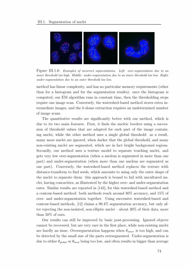
III.1. Segmentation of nuclei
Figure III.1.6: Examples of incorrect segmentations. Left: over-segmentation due to an
inner threshold too high. Middle: under-segmentation due to an inner threshold too low. Right:
under-segmentation due to an outer threshold too low.
method has linear complexity, and has no particular memory requirements (other
than for a histogram and for the segmentation results): once the histogram is
computed, our EM algorithm runs in constant time, then the thresholding steps
require one image scan. Conversely, the watershed-based method stores extra in-
termediate images, and the h-dome extraction requires an undetermined number
of image scans.
The quantitative results are significantly better with our method, which is
due to its two main features. First, it finds the nucleic borders using a succes-
sion of threshold values that are adapted for each part of the image contain-
ing nuclei, while the other method uses a single global threshold: as a result,
many more nuclei are ignored, when darker that the global threshold, and many
non-existing nuclei are segmented, which are in fact bright background regions.
Secondly, our method uses a texture model to separate touching nuclei, and
gets very low over-segmentation (when a nucleus is segmented in more than one
part) and under-segmentation (when more than one nucleus are segmented as
one part). Conversely, the watershed-based method replaces the texture with
distance-transform to find seeds, which amounts to using only the outer shape of
the nuclei to separate them: this approach is bound to fail with uncultured nu-
clei, having concavities, as illustrated by the higher over- and under-segmentation
rates. Similar results are reported in [143], for this watershed-based method and
a contour-based method: both methods reach around 80% accuracy, and 15% of
over- and under-segmentation together. Using successive watershed-based and
contour-based methods, [12] claims a 99.4% segmentation accuracy, but only af-
ter rejecting the non-isolated, non-elliptic nuclei – about 30% of their data, more
than 50% of ours.
Our results can still be improved by basic post-processing. Ignored objects
cannot be recovered, but are very rare in the first place, while non-existing nuclei
are hardly an issue. Oversegmentation happens when θinner is too high, and can
be detected by the small size of the parts oversegmented. Under-segmentation is
due to either θglobal or θlocal being too low, and often results in bigger than average
74

III.1. Segmentation of nuclei
objects, which could be detected as such and processed with higher thresholds.
Examples of under and over-segmentation are shown in Figure III.1.6.
75

III.2. Segmentation of telomeric probes
Once the nuclei are segmented, their telomere content is evaluated: this is per-
formed by segmenting the fluorescent probes in the green channel. The probes
appear as small spots of about twenty pixels in area. Background illumination
is observed around the probes as well; however we cannot apply the same seg-
mentation method as for the nuclei. This is for practical reasons: for a typical
image, the nuclei represent 8% of the pixels in the image, and the illuminated
background about 50%, but the probes only represent 0.3%, and the background
around them, 2%. Adjusting our model based on so few pixels would not be
reliable enough.
As explained in Chapter I, the FITC images can be affected by foreground
noise: unattached and unwashed clustered probes can appear on some images,
sometimes overlapping a nuclei in the DAPI channel. This is illustrated in Fig-
ure III.2.1. Although it is not frequent, in about one in thirty images, segmenting
it as valid attached probes would affect the reliability of our system, which is
meant in the long run to identify rare fetal cells based on their probe contents.
Existing methods of probe segmentation fall in two categories. Some meth-
ods are meant to count the number of probes, usually to detect aneuploidies [92,
113, 123, 167]. These methods are not applicable for our task, where the total
segmented intensity is more relevant than the exact number of probes. The
other category is concerned with a quantitative evaluation of fluorescence in
nuclei, which is our goal, and especially to assess the telomere length. As ex-
plained in Chapter I though, such methods usually rely on cultured metaphase
nuclei for quantitative FISH [6, 86, 112, 128,183]. Methods used to automate the
segmentation of probes prior to quantitative evaluation include: image smooth-
ing and top-hat transform [122], background subtraction, image smoothing and
watershed [86], background subtraction, image smoothing and threshold [112],
background subtraction [128], image smoothing and thresholding [139]. These
methods, however, are not meant to segment images with the foreground noise
76

III.2. Segmentation of telomeric probes
described above, and would segment it as valid signal. Further processing to
classify segmented shapes would be required, as in [92, 93]. This require tuning
or learning, bringing additional issues of classification to our segmentation task.
Instead, we developed a segmentation method robust to foreground noise, based
on a novel dome-finding algorithm.
Figure III.2.1: Examples of foreground noise.
III.2.1 Dome-finding algorithm
Our new method is based on the following observations. Background noise is
caused by random reflections of light towards the optics, and does not reflect any
material structure. In the same way, unwashed probes are randomly clustered,
and cause random values on the resulting image. Probes attached to telomeres,
however, have a consistent spatial structure, reflecting that of telomeres. In in-
terphase nuclei, telomeres are wrapped [24], forming small ovoid structures. Con-
sequently, when imaged with FISH, FITC probes attached to telomeres appear
as small spots with a bright centre, due to higher concentration of fluorescent
material, and an intensity decreasing away from the centre. This structure of
local intensities is consistent for all attached probes, regardless of their actual
intensity values. This is what we use to discriminate between valid probes and
noise, both background and foreground.
A local maximum is a pixel which value is higher than its 8 nearest neigh-
bours, in our context. Considering a random distribution of integer values in
two dimensions, there is no correlation between neighbouring pixels. On such
a distribution, the probability of finding a local maximum is equivalent to that
of finding the maximum of nine random numbers, i.e. 19≈ 11%. Consequently,
in background and foreground regions of FITC images, the proportion of local
maxima is approximately 11%. In regions showing probes however, there is one
local maximum within the two scores of pixels showing the probe: the proportion
of local maxima is around 120
= 5%. We set the average value 8% = 225
as the
threshold separating these two proportions. An image region containing more
77

III.2. Segmentation of telomeric probes
than 2 local maxima within 25 neighbouring pixels is considered as noise; if it
contains 1 or 2 local maxima, it is considered as containing a probe.
Probe segmentation requires more than selecting potential regions of interest,
or than finding local maxima. As we are interested in the total probe intensity,
we need to segment all the pixels forming a probe signal. Using the landscape
metaphor, probes are dome-shaped, circular and no more than 3 pixels in radius.
They are centred around a local maximum, in a region containing at most 2 local
maxima within 25 pixels.
To segment probes efficiently under these constraints, we use a novel dome-
finding algorithm. Briefly, it works as follows: the image is scanned once, and
every local maximum is considered as a dome centre. The surrounding pixels are
inspected, and marked as part of the dome if they follow a dome-shape criterion.
With this marking, the resulting dome will be small in noisy regions and large on
probes. Translating the proportion constraint described above into a dome size
constraint, only domes of a given size are selected as valid probe segmentation.
We now detail these steps.
Dome construction: Around each local maximum, we consider three sets of
neighbouring pixels at increasing distances. They approximate the shape of a
probe, and are illustrated in Figure III.2.2 by three different shades of gray
around the local maximum marked in black. Each set forms a level set of the
dome, referring to the original topological definition of level sets, not to the
level-set segmentation method. The first level set consists of the 8 closest pixels:
LS1 = p, d∞(p, pM) = 1. In the second level set are the twelve closest pixels
that are not already in LS1 : LS2 = p, p /∈ LS1 ∧ d1(p,LS1 ) = 1. A similar def-
inition holds for the third level sets: LS3 = p, p /∈ LS1 ∪ LS2 ∧ d∞(p,LS2 ) = 1.Each pixel in the sets LS1 and LS2 is assigned three neighbours, as indicated by
the arrows in Figure III.2.2. We refer to them as downhill neighbours. When the
level sets around a local maximum are inspected, a pixel is marked as part of the
dome if its value is higher than its downhill neighbours. Once all pixels in level
sets 1 and 2 have been inspected, the constructed dome is defined as the pixels
marked.
The use of downhill neighbours in building the dome is motivated by the fol-
lowing reason. A straightforward criterion to build a dome would be: min LSi ≥max LSi+1. It would only segment domes with circular symmetry though. How-
ever when wrapped, telomeres are not perfected spheres, but might be elongated
ellipsoids. As a result, the light intensity at one part of the dome might be higher
than at the opposite part. Our criterion is robust to such cases, as it is only
sensitive to the variations of intensity in subparts of the dome.
78

III.2. Segmentation of telomeric probes
Figure III.2.2: Dome model: the three level sets around a local maximum are indicated in
different shades of gray. All downhill neighbours are indicated with arrows.
Dome selection: Domes are constructed around every local maximum in the
image, but those in noisy regions have to be rejected. The criterion defined above
can be translated as follows. Let us consider a 5× 5 square of pixels centred on
a local maximum. This square either contains:
- One local maximum: the region contains a probe, centred on the maximum,
and by construction the dome marks all pixels on it. It should be kept as a
valid probe.
- Two local maxima: this is still considered as a region showing probes, so
the dome should be kept. However, the pixels in-between the two maxima
will follow a saddle shape, and cannot be marked as part of the dome.
This interference between the two domes is restricted to one quarter of the
dome though (see Figure III.2.3). At most 75% of level sets 1 and 2 can be
marked.
- More than two local maxima: the region is now considered as noisy. The
combined effect of the two extra local maxima will cause more than one
quarter of level sets 1 and 2 to be unmarked.
As a result, we use the following criterion. A dome is kept as segmenting a valid
probe if at least 75% of the pixels in LS1 and at least 75% of those in LS2 are
marked; otherwise it is rejected as noise. Examples of constructed domes are
shown in Figure III.2.4: only the one in the middle is kept.
III.2.2 Results and discussion
The categories of segmentation result presented in the introduction and used for
the segmentation of nuclei do not correspond well to the segmentation of probes.
What is to be evaluated is the total fluorescence segmented within a nucleus,
more than the number of probes. Our method prevents undersegmentation and
79

III.2. Segmentation of telomeric probes
Figure III.2.3: Pixels affected by the presence of another local maximum, in red: at most one
quarter of pixels in level sets 1 and 2 are affected and cannot be marked as part of the dome.
Figure III.2.4: Domes constructed in image regions containing: background noise (left), probe
(middle), foreground noise (right).
oversegmentation by design, as it keeps probes at a given size. The possible out-
comes are simply as follows: a probe is either correctly segmented or missed, and
noise may be segmented as a probe. The less severe errors are the segmentation
of background noise and the missing of a dark probe. The more severe errors are
the missing of a bright probe, and the segmentation of foreground noise.
We do not use Receiver-Operator Characteristic (ROC) curves in this sec-
tion for the following reasons. ROC curves represent the true positive rate and
false positive rate achieved by a classifier when varying one of its parameters.
It requires a two-class classifier and supposes that each item can be classified
manually into one category. In our case, considering pixel segmentation as a two-
class labeling classification is not adapted: while the pixels at the core of a probe
are easily distinguishable, some pixels at the edge of a probe may be classified as
background or probe by different experts. This amounts to saying that not all the
pixel labels have the same significance for the final results. Another possibility
would be to consider probe classification as a two-label classification. The first
issue with this approach is the definition of a probe: using connected components
in the segmented image is bound to fail for methods like the top-hat transform,
as can be seen in Figure III.2.6, bottom right-hand corner: nearby probes tend to
be merged into single connected component. The second issue is that false pos-
itives (noise segmented as probe) falls in two important categories: background
noise segmented as probe is not an issue for the application we are considering,
while foreground noise segmented as probe is a major problem. In the same vein,
80

III.2. Segmentation of telomeric probes
Figure III.2.5: Example of a probe missed with our dome-finding segmentation method.
false negatives need to be classified in two categories: missing dark probes is not
very important, while missing bright probes is problematic. For these reasons, we
ruled out the use of ROC curves to analyse the probe segmentation results. The
threshold parameter, set to 75%, was empirically found to offer a good quality of
results, based on the severities presented above.
Table III.2.1: Results of the telomere segmentation.
Segmentation Dome-finding Top-hat
Number of probes 1,000 1,000
Correctly Segmented 993 931
Dark probes missed 5 62
Bright probes missed 2 7
The results of our dome-finding method, as well as a top-hat segmentation
method (see Section II.1 on Shape extraction, page 20, for details on the top-hat
segmentation), are listed in Table III.2.1. Our method correctly segments 99.3%
of probes. An example of missed probe is shown in Figure III.2.5. It performs bet-
ter than the top-hat segmentation. Figure III.2.6 shows a comparison of the two
methods. In addition, our dome-finding method segments background noise as
probe with a frequency of about 0.1%, and leaves foreground noise unsegmented.
By contrast, the top-hat method never segments background noise, but always
segments foreground noise, as illustrated in Figure III.2.7. Our dome-finding al-
gorithm is reliable to segment probes and count them. In the next part we use it
in addition to our nucleus finding algorithm to compare the telomeric intensities
from different individuals.
81
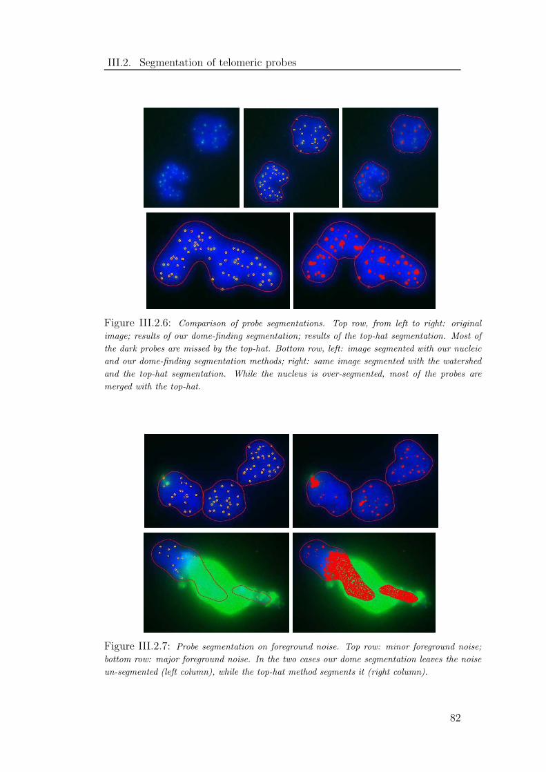
III.2. Segmentation of telomeric probes
Figure III.2.6: Comparison of probe segmentations. Top row, from left to right: original
image; results of our dome-finding segmentation; results of the top-hat segmentation. Most of
the dark probes are missed by the top-hat. Bottom row, left: image segmented with our nucleic
and our dome-finding segmentation methods; right: same image segmented with the watershed
and the top-hat segmentation. While the nucleus is over-segmented, most of the probes are
merged with the top-hat.
Figure III.2.7: Probe segmentation on foreground noise. Top row: minor foreground noise;
bottom row: major foreground noise. In the two cases our dome segmentation leaves the noise
un-segmented (left column), while the top-hat method segments it (right column).
82

III.3. Comparison of telomere
intensities
III.3.1 Data set and calibration
We now use the two segmentation methods together to proceed to the cytometric
task described in Chapter I. The final goal of this task is to identify a fetal nucleus
within several thousand maternal nuclei, based on the fluorescent intensity of
telomeric probes visible in all the nuclei. Before this can be achieved, we need to
evaluate whether probe intensity is significantly different in nuclei sampled from
people at different ages.
As a pilot study to assess the reliability of the telomeric probe intensity as
an indication of a person’s age, four blind trials were conducted, resulting in four
sets called MT002, MT004, MT007 and MT024. For each trial, three individuals
(except in set MT007 with only two individuals) were sampled for telomeres,
which were then processed and imaged in similar conditions. The individuals
within each set, named MT0xx-1, MT0xx-2 and MT0xx-3, differ in age. One of
them is a foetus, one is an adult female and one (except in set MT007) is an
adult male. As a blind trial, we do not known which individual corresponds to
which name. The trial consists in processing the images from each individual in
the same way, as detailed before, so as to measure the average probe intensity in
each nucleus from each individual. Several hundred nuclei are to be segmented
for each individual, and the resulting distribution of the average probe intensities
will be represented with one histogram per individual. As explained in Chapted I,
the telomeric length decreases with a person’s age, inducing a decrease of probe
intensity, so it is expected that one individual (the foetus) in each set will show
higher probe intensities than the other two.
In addition, the imaging quality of the samples can be estimated, using the
number of probes segmented per nucleus. With 23 pairs of chromosomes, a typical
83

III.3. Comparison of telomere intensities
Set Individual # Images Set Individual # Images
MT002 MT002-1 228 MT007 MT007-1 247
MT002-2 198 MT007-2 180
MT002-3 297
MT004 MT004-1 152 MT024 MT024-1 70
MT004-2 273 MT024-2 70
MT004-3 382 MT024-3 69
Table III.3.1: Number of images for each individual in our data set.
nucleus contains 92 telomeres. However, no nucleus contains 92 probe signals.
This is mostly because the telomeres tend to cluster [186], and partly because of
imaging quality. In particular blur reduces the number of visible and segmentable
probes. As a rough quality estimation, nuclei showing above 20 probes can be
considered as correctly imaged [186], while the others may suffer from unmarked
telomeres, blur or missed segmentation. Again, the distributions of the number
of probes segmented per nuclei will be represented with histograms, one per
individual in each set. For each individual, one slide of uncultured interphase
leucocytes was prepared for FISH imaging: the numbers of images, in pairs DAPI-
FITC, available for each individual are listed in Table III.3.1. The whole data
set was processed with the segmentation methods described in the previous two
sections. Nuclei were segmented first, then the telomeric probes inside them were
also segmented.
The FITC probes used attach to small regions of the telomeres: the longer the
telomeres, the more probes are attached. However, the probes cannot be used to
measure directly telomere length. In interphase nuclei, telomeres are wrapped,
and at the scale used for imaging, probes are about two or three pixels in diameter.
A change in length by 30% would affect the size of the probe signal by less than a
pixel. Instead, the pixel intensity can be used to measure the energy emitted by
a probe. Two measures can be performed after segmentation: the average probe
intensity f i and the average background intensity bi in a nucleus i. Considering
two individuals 1 and 2 in a given set, we note these measures respectively f i1, b
i1,
f i2, b
i2. Let f1, b1, f2, b2 be the average values of these measures.
A significant issue arises when measuring pixel intensities to compare different
individuals. Even though each individual’s sample within a set was processed in
the same way, they were imaged separately, at different times. The imaging
conditions, such as the surrounding illumination, the excitation intensity or the
exposure time may be slightly different for different individuals within a set, with
a direct impact on image intensity. Before comparing the probe intensities from
different individuals, the FITC intensities f1, b1, f2, b2 have to be calibrated.
84

III.3. Comparison of telomere intensities
To calibrate segmented FITC images from the different individuals of a set,
we use the following model. Considering two individuals 1 and 2, let I1 and I2 be
their average probe intensities. We model the background fluorescence as additive
background noise; since their samples were processed in the same way, we consider
that the FITC background has the same average intensity for both of them, and
note it B. As a result, the intensity at a probe is I1 + B for individual 1, and
I2 +B for individual 2, and the background intensity is B for both of them. The
excitation intensity and the exposure time induce a multiplicative gain: let α1 be
the gain for individual 1, and α2 that for individual 2. After segmentation of the
FITC images, the average intensities measured in the background of foreground
are:
individual 1 individual 2
background b1 = α1 B b2 = α2 B
foreground (probe) f1 = α1 · (I1 +B) f2 = α2 · (I2 +B)
(III.3.1)
With this model, calibrating the intensities can be achieved by multiplying
the foreground intensities of individual 2 by α1
α2. This ratio, which we refer to
as calibrating factor, could be obtained directly from the average background
intensities b1 and b2, defined in Equation III.3.1. Such a measure would not be
precise though, because of the wide range of values taken by the bi. A more
precise measure can be performed as follows.
The values measured after segmentation for individual 1 are f i1 and bi1 in each
nucleus i. With the model above, the average of the differences f i1 − bi1 is α1 I1.
The average of the ratiosf i1
bi1
is I1+BB
, so the average of the quantitiesf i1
bi1
− 1 is I1B
.
This way, in the two-dimensional graph
(x =
f i1
bi1− 1 , y = f i
1 − bi1)
(III.3.2)
the slope of a linear interpolation is α1 I1 · BI1
= α1 · B. Plotting the same graph
for individual 2 gives access to α2 · B, as the slope of the linear interpolation of
the samples. Finally, the ratio of these two slopes gives the calibrating factor α1
α2
for individual 2.
The graphs described in Equation III.3.2 and the calibrating factors are pre-
sented in Figure III.3.1 for the four sets. In each set, an individual ref is chosen
as a reference, and its measured intensities are not modified. For the other in-
dividuals oth of the set, the measured intensities foth and both are calibrated, by
multiplying them with the corresponding calibration factorαref
αoth, listed in Fig-
85
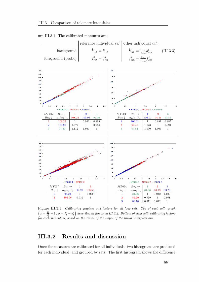
III.3. Comparison of telomere intensities
ure III.3.1. The calibrated measures are:
reference individual ref other individual oth
background biref = biref bioth =αref
αothbioth
foreground (probe) f iref = f i
ref f ioth =
αref
αothf ioth
(III.3.3)
MT002 Bαi → 1 2 3
Bαj ↓ αi/αj ց 108.22 100.91 97.30
1 108.22 1 0.932 0.899
2 100.91 1.072 1 0.964
3 97.30 1.112 1.037 1
MT004 Bαi → 1 2 3
Bαj ↓ αi/αj ց 106.01 94.41 93.84
1 106.01 1 0.891 0.885
2 94.41 1.123 1 0.994
3 93.84 1.130 1.006 1
MT007 Bαi → 1 2
Bαj ↓ αi/αj ց 94.20 103.56
1 94.20 1 1.099
2 103.56 0.910 1
MT024 Bαi → 1 2 3
Bαj ↓ αi/αj ց 81.36 84.79 83.78
1 81.36 1 1.042 1.030
2 84.79 0.959 1 0.998
3 83.78 0.971 1.012 1
Figure III.3.1: Calibrating graphics and factors for all four sets. Top of each cell: graph(x =
fi
1
bi
1
− 1 , y = f i1 − bi
1
)described in Equation III.3.2. Bottom of each cell: calibrating factors
for each individual, based on the ratios of the slopes of the linear interpolations.
III.3.2 Results and discussion
Once the measures are calibrated for all individuals, two histograms are produced
for each individual, and grouped by sets. The first histogram shows the difference
86

III.3. Comparison of telomere intensities
f i − bi per nucleus. Using the model presented above, this quantity is:
f i − bi = αref · I i (III.3.4)
where I i is the average probe intensity in nucleus i. The factor αref is unknown,
but is constant within a set. This measure can be used to compare the average
probe intensities per nucleus for all individuals in a set. The histograms of all
individuals are presented in the left column of Figure III.3.2. To evaluate the
quality of the images, we also construct the histograms of the number of seg-
mented probes per nucleus, in the right column of Figure III.3.2, as explained in
the previous section.
In the set MT002, the number of probes in MT002-3 is below 20 for about
two third of the nuclei. Should this individual be left out, for low quality reasons,
the differences of calibrated intensities show a clear separation between MT002-1
and MT002-2.
In the set MT004, the imaging quality is poor for MT004-1 and MT004-3,
and average for MT004-2 judging from the relatively small number of probes
segmented in nuclei. In addition, although it does not appear on the histogram,
more than 80% of the nuclei in MT004-3 have a zero average difference of cali-
brated intensities. This happens when probes are visible as dome structures, but
have the same average intensity as the background, due to blur. Consequently,
although MT004-2 tend to show brighter probes, those measured are strongly
affected by imaging conditions in set MT004.
Set MT007 only contains two individuals. The relatively high number of
probes segmented per nucleus for the two individuals indicates a relatively good
imaging quality. Probes in MT007-2 are generally brighter than in MT007-1.
Actually, because of practical issues, MT007-2 was imaged several days after its
preparation. As a result, the fluorescence of probes had reduced before imaging.
This causes the differences of calibrated intensities to shift towards lower values,
and increase the overlap with MT007-1. It is expected that without the imaging
delay, the overlap would have been reduced.
Finally, all three individuals in set MT024 have an average imaging quality.
Although less nuclei were segmented in MT024-2 than in the other cases, they
tend to show brighter probes.
To conclude, judging from the histograms on the left of Figure III.3.2, show-
ing the differences of calibrated foreground and background intensity per nucleus,
one individual in each set appears to have brighter probe signals than the others.
They are MT002-1, MT004-2, MT007-2 and MT0024-2, shown in red. However,
there is still overlap with the other individuals. One cause is the imaging qual-
ity, in particular recurring blur in FITC images. Although these results show
a promising trend, more data from more individuals would be needed before
87

III.3. Comparison of telomere intensities
Figure III.3.2: Calibrated probe intensity and number of probes per nucleus, for the four blind
trials. Left column: histogram of the average probe intensity per nucleus, in arbitrary units.
In each set the distribution of one individual (shown in red) is centred on higher intensities
than the other individuals, proving it contains brighter probes. Right column: histogram of
the number of segmented probes per nucleus. Nuclei with less than 20 probes suffer from low
imaging quality, and their average probe intensity is unreliable. This is especially the case in
MT002 and MT004.
88

III.3. Comparison of telomere intensities
drawing conclusions on the quality of telomere probe intensity as a measure to
distinguish individuals’ ages.
89

Summary
In this chapter we have detailed our new segmentation methods, presented a
quantitative comparison of our nucleic segmentation with the widely used wa-
tershed method, and shown an application of our methods for medical research.
The nucleic segmentation method we developed is based on a new model of the
image histogram, achieves a 99.3% accuracy and, to the best of our knowledge,
is more robust and automatic than previously published work on this field. As
for the telomere probes, our method is robust against all sources of noise, and
is also 99.3% accurate. The application presented here shows that the telomere
probe intensity is a potentially promising criterion to differentiate individuals’
ages, but it requires good imaging conditions. In particular, each sample should
be processed and imaged similarly and during the same period of time. Although
major improvements can be achieved with a higher imaging quality, other post-
segmentation techniques can be devised to increase the quality of the results.
Selecting nuclei based on their usability is one approach, which we present in
Section V.3 as future work.
Regarding computer vision, the nucleus segmentation method developed was
evaluated on our whole data set, and other methods on a subset. These evalua-
tions were performed visually by the author, based on some examples of correct
segmentation provided by cytometrists. This is a time-consuming process, which
depends on the evaluator’s subjectivity. In the next chapter, we present a novel
framework to define segmentation references, possibly combine multiple references
from different users, and automatically evaluate a segmentation method against
these references, with a single measure.
90

Chapter IV
Evaluation of a Segmentation
Method
91

As explained in the introduction, we are interested in evaluating segmentation
methods in terms of discrepancy [201]. It consists in comparing a segmented shape
with a reference. In this chapter we address the issues related to discrepancy
evaluation, in a medical imaging context, detailed in Section I.2.3. Briefly, the
four issues we identified are:
- A need for quantitative as well as qualitative description of segmentation
results, with the following categories: correct, over- and under-segmented,
missed and noisy segmented objects.
- A definition of correctly segmented object which is less strict than a perfect
match with a reference: in particular partial volume effect and blur can
cause an object’s boundaries to span several pixels, so a segmented object
may be correct while differing from the reference by several pixels.
- A possibility to combine multiple references into a single one: references
drawn by different users or by one user at different times may differ slightly
at some parts of an object, yet eventually only one reference is to be used.
- A clarification in the presentation of evaluation results: for example the
proportion of correctly segmented references may differ from the proportion
of objects correctly segmenting a references, though both may be called
success rates.
We introduce a novel method, called Confidence Maps Estimating True Segmen-
tations (Comets), to store segmentation references for medical imaging, combine
multiple references, and measure the discrepancy between a segmented object and
a reference. The key novelty of our model is to store local confidence factor along
a reference. Local confidence is computed from user input, and is used to define
a new discrepancy measure. To help resolve an ambiguity inherent to evaluation,
we also introduce two complementary ways to present discrepancy results: the
reference and user viewpoints. We show that, with a single measure, our method
allows a qualitative and quantitative evaluation of a segmentation method, and
compare it with existing metrics.
We start with a review of existing work addressing the issues mentioned above,
and then present our model, Comets. We detail how to encode one reference, how
to combine multiple references and how to evaluate a segmentation method. We
also compare our evaluation method with existing metrics.
92

IV.1. Existing work
IV.1.1 Measures for discrepancy evaluation
Given a reference and a segmented shapes, there are several ways to assess their
match. Different measures have been published and used. Many of them are based
on low-level vision metrics. Two such families of measures are based on ratios of
numbers of pixel (area-based), and on distances between shapes (distance-based).
Let C be a reference, and S be a corresponding segmented shape. Let AC
be the area of C in pixels, and Ci1≤i≤n the set of n pixels at the border of C.
Similarly, let AS be the area of S, and Sj1≤j≤m the set of m pixels at the border
of S. Examples of area-based measures are:
Sensitivity, RUMA: true positive ratio [185], or Relative Ultimate Measure-
ment Accuracy [54, 156, 202]:
Sensitivity = RUMA =AS∩C
AC. (IV.1.1)
Specificity: true negative ratio [185]:
Specificity =AImage−S∪C
AImage−C. (IV.1.2)
RAO: Relative Area Overlap [54]:
RAO =AS∩C
AS∪C
. (IV.1.3)
DSC: Dice Similarity Coefficient [205]:
DSC =2×AS∩C
AS + AC. (IV.1.4)
93

IV.1. Existing work
Performance: [102]:
Performance = 1−√w2(1− TP)2 + (1− w)2FP2 , (IV.1.5)
where: w = AC
AImageis the proportion of foreground pixel in the image, TP =
AS∩C
ACis the true positive ratio, and FP = AS−C
AImage−Cis the false positive ratio.
Each measure indicates a fraction of misclassified pixels: for instance sensitivity
gives an idea of oversegmentation, and specificity of undersegmentation; others
combine the two. However, the severity of the segmentation errors can be difficult
to evaluate based on these ratios. In particular, the specificity depends on the
background size, which in our case is more than a million pixels: even a severe
nucleus segmentation error will have a high specificity. Also, the geometry of the
misclassified regions is not taken into account: this makes a tolerance margin
difficult to use with the area-based measures. Pixels ratios depend on the object
sizes, some even on the image size, and do not easily take into account tolerance
margins.
Examples of distance-based measures are:
Hausdorff Distance: [11, 54, 87, 136]:
HaussMax = max1≤i≤n
min
1≤j≤md(Ci, Sj)
(IV.1.6)
where d(P,Q) is the Euclidian distance between pixels P and Q.
Hausdorff Mean Distance and Standard Deviation: [87, 136]:
HaussMean =1
n
n∑
i=1
min1≤j≤m
d(Ci, Sj) (IV.1.7)
HaussStdDev =1
n(n− 1)
n∑
i=1
(min
1≤j≤md(Ci, Sj) − HaussMean
)(IV.1.8)
Distances measures depend directly on the geometry of the misclassified regions:
it is easier to include tolerance margins around a reference segmentation. How-
ever, these distances are measured in pixels. Interpreting their values to infer the
severity of an incorrect segmentation require to know the typical size of an ob-
ject of interest, which may vary across samples. Distinguishing between over- and
under-segmentation is difficult with the definitions above, as the distance between
pixels is symmetric. It may be done by introducing a sign in the computation:
d(Ci, Sj) =
+‖Ci − Sj‖2 if Si ∈ C−‖Ci − Sj‖2 else
(IV.1.9)
94

IV.1. Existing work
though it requires extra care when computing the maximum, mean and deviation
of the distance distribution between the shapes.
The measures above do not require any parameter, and are straightforward to
compute. However, none of them seems to be satisfying as a standalone measure:
at least two needs to be combined to obtain quantitative and qualitative evalu-
ation of a segmentation result. Interpretation of quantitative results requires an
external reference as well.
Other measures are based on fuzzy systems [43, 174]. They rely on a fuzzy
extension of segmentation, where pixels at the border of objects are assigned
fractional labels. The measures defined above can be extended in a fuzzy frame-
work. However, these measures introduce parameters, such as the extent of fuzzy
boundaries and the relative weights of different labels. These parameters have to
be tuned, which may add subjectivity the evaluation process, and raises issues
when interpreting and comparing evaluation results.
Finally, an approach to evaluation has been to use several metrics at the same
time [54, 87, 136, 174]. Though it gives more data, it leads to more questions on
how to combine them, or which ones are more informative. Basically, it amounts
to representing segmentation results in a space with many dimensions, some re-
stricted to values between 0 and 1, some to positive values, other to any values,
and each one having its own external reference for interpretation. It adds to the
complexity of evaluating a single segmentation method, but also of comparing
different methods, or tuning of a method’s parameters. In this chapter we intro-
duce a single measure, which can be interpreted qualitatively and quantitatively
with no external reference.
IV.1.2 Combination of multiple references
Manual references, however useful for evaluation, are subject to inter- and intra-
user variability. Different experts, or one expert at different times, may disagree
on some parts of the objects’ boundaries, while agreeing on others. This calls for
a way to combine multiple segmentations into a single reference. Ideally it should
keep as much expert knowledge as possible.
Different methods have recently been published. Rohlfing et al. [145] aver-
age the Euclidian distances between the shapes, as in [173]. Kim et al. [76] use
Weiner measures instead of Euclidian. The results obtained, however, do not
reflect how different the expert segmentations were, by treating equally the zones
of agreement and disagreement between experts. In case two references differ
significantly in one region, the constructed reference will be far from both, and
the evaluation measure of the original references will be high, even though both
95

IV.1. Existing work
may be correct.
In an area-based approach, STAPLE [185] optimises the references’ specifici-
ties and sensitivities, based on a Markov Random Field (MRF). These area-based
ratios depend on the object and image sizes though, and MRF are used by some
segmentation methods [13, 31]. It requires the tuning of many parameters, uses
criteria that are size-dependent, and violates the independence criterion described
by Lehmann in [91]. It may be biased favorably for segmentation methods based
on MRF, and for area-based discrepancy measures.
In this chapter we present a novel way to encode expert references, and use
it to define a new single metric for discrepancy evaluation, size-independent,
parameter-free and intuitive to interpret. We detail how to combine multiple ref-
erences with Comets, with no parameter nor segmentation model, while keeping
more information than a single shape can.
96
IV.2. Comets: a novel method of
referencing
We present our novel model, Confidence Maps Estimating True Segmentation,
Comets. We explain how to encode a segmentation reference with local confi-
dence, and how to visualize it with confidence maps. Then we detail how to
combine multiple segmentations using local confidence. Finally we present the
new discrepancy metrics associated with our model.
IV.2.1 Encoding a reference with local confi-
dence
The user input consists in drawing a continuous border around the object, and
selecting pixels inside and outside the object (see Figure IV.2.1, left, and Fig-
ure IV.2.2, middle), according to the following criteria. We refer to the pixels on
the border as edge pixels, and to the pixels selected around the object as outer
and inner limit pixels. Outer limit pixels (respectively inner limit pixels) are
examples of pixels closest to the border that the user is certain belong to the
background (respectively to the object). The number of limit pixels to select
depends on the local variations of confidence, the local variations of blur, or the
presence of touching objects. They are used only to define the confidence that
the border is locally correct. Their selection is thus easier and less critical than
landmarks.
Using this user input, the local confidence factors are computed as explained
below and illustrated in Figure IV.2.1. Every edge pixel is assigned an inner and
an outer confidence factor, respectively IC and OC . First, for the edge pixels E
that are the closest to outer limit pixels, at distance d (see Figure IV.2.1, middle):
OC (E) = d (IV.2.1)
97

IV.2. Comets : a novel method of referencing
E1
d1 outer limit pixels
edge pixels E2
d2
OC (E1)=d1
OC (E2)=d2
s1
s2E
OC (E) = d1s2+d2s1
s1+s2
d
E
P
Conf (P )=− dOC (E)
Figure IV.2.1: Construction of a Comets. Left: User input. Middle: Outer Confidence
factors assigned to the edge pixels closest to outer limit pixels then interpolated linearly along the
curvilinear coordinate. Right: Confidence of any outside pixel P , based on the Outer Confidence
factor of the closest edge pixel.
Then, the outer confidence factors of the remaining edge pixels are computed
using the existing values, with a linear interpolation along the curvilinear distance
between the edge pixels. Let E be an edge pixel, and let E1 and E2 be the pixels
already having outer confidence factors d1 and d2 closest to E, at curvilinear
distance s1 and s2 (see Figure IV.2.1, middle). The outer confidence factor of E
is defined as:
OC (E) =d1 s2 + d2 s1
s1 + s2(IV.2.2)
The same method of sampling and interpolation is used to compute the inner
confidence factor.
Once the confidence factors are computed, the confidence map of the reference
is computed by assigning a confidence Conf to every pixel P . If P is an edge
pixel,
Conf (P) = 0 (IV.2.3)
If P is inside the shape, let E be the edge pixel closest to P , at distance d:
Conf (P) =d
IC(E)(IV.2.4)
Finally, if P lies outside the shape, and the closest edge pixel is at distance d (see
Figure IV.2.1, right):
Conf (P) = − d
OC(E)(IV.2.5)
Qualitatively, the confidence assigned to any pixel P can be interpreted as:
if Conf (P ) ≥ 1 : P is strongly believed to be part of the object
if −1 < Conf (P ) < 1 : P is believed to be on or close to the border
if Conf (P ) ≤ −1 : P is strongly believed to be out of the object
Quantitatively, the higher |Conf (P )|, the more confident the expert is that P
belongs to the object or to the background. The pixels with low confidence,
between -1 and 1, form a band around the object border (see white band on
Figure IV.2.2, right, and Figure IV.2.3, right). The band width reflects the
expert’s local confidence in the true border location: the narrower the band is
98

IV.2. Comets : a novel method of referencing
limit pixels
edge pixels
3210-1-2-3
Confidence
Figure IV.2.2: Construction of a Comets. Left: original image. Middle: user input. Right:
the corresponding Comets.
locally, the more confident the expert is that the border drawn corresponds to
the actual border.
With the user input and formulas detailed above, single references with local
confidence are encoded as Comets. For storage optimization, only the edge pixels’
coordinates and confidence factors are stored. The actual confidence map can be
recomputed when needed, at any size, with the construction above. We now
describe how to combine multiple segmentations of an object with Comets.
IV.2.2 Combining multiple segmentations into
a single reference
Our novel approach to combine multiple segmentations is to weight them with
the local confidences. This is done by averaging the confidence maps defined
above. Let Ci1≤i≤n be the set of n expert segmentations to combine, encoded
as Comets. Let
Ω = P , ∃ i : Conf i(P )≥−1 (IV.2.6)
where Confi(P ) is the confidence of pixel P with respect to Ci. All pixels out-
side Ω are confidently considered as background by all the experts, so they are
discarded for the rest of the construction. We define the final confidence map on
the domain Ω as the average of all the experts’ confidence maps:
∀P ∈ Ω,Conf (P ) =1
n
n∑
i=1
Conf i(P ) . (IV.2.7)
We define the set of final edge pixels E , the set of final outside confidence pixels
O, and the final inside confidence pixels I as:
E = P ∈ Ω : Conf (P ) = 0 (IV.2.8)
O = P ∈ Ω : Conf (P ) = −1 (IV.2.9)
I = P ∈ Ω : Conf (P ) = 1 (IV.2.10)
The confidence factors of the final edge pixels are then computed as detailed
in Section IV.2.1. An example of segmentation combination is shown in Fig-
99

IV.2. Comets : a novel method of referencing
3210-1-2-3
Confidence
Figure IV.2.3: Combining multiple segmentations. From left to right: original image; input
from expert 1; input from expert 2; resulting average Comets. The zones of disagreement have
lower confidence, as reflected by the width of the white band around the border.
ure IV.2.3. Notice that the zones of disagreement receive a lower confidence that
the zones of agreement.
100

IV.3. Evaluating a segmentation
method with Comets
We start by defining the discrepancy measure associated to Comets, for a single
segmented object against a single reference. We show the results obtained on a
test data set, to compare different discrepancy measures. Then, we detail how
to present complete results of a segmentation method, involving several objects
against several references, from a reference and from a user viewpoint. Finally we
illustrate how Comets can be used to tune a segmentation method’s parameters
based on a large number of references.
IV.3.1 Evaluation of a single segmented object
Let C be a reference encoded as Comets, with confidence Conf , and let ObjC =
P :Conf (P ) ≥ 0 be the set of pixels referenced as the object. Let S be the set
of pixels segmented as the object, and Mis = (S ∪ObjC)− (S ∩ObjC) the set of
mislabeled pixels. The segmentation error of S against C is defined as:
error(S,C) =
∞ if S ∩ ObjC =∅Conf (P0), P0 =arg maxP∈Mis|Conf (P )| else.
(IV.3.1)
Intuitively, if there is no overlap between the segmented object and the reference,
they are not related and the error is∞. Otherwise, mislabeling pixels of low con-
fidence only (near the object boundary) leads to a small error, while mislabeling
higher confidence pixels causes a greater error. Moreover, the value of this error
can be interpreted in terms of qualitative segmentation error [66], as follows. A
shape with error 0 is a perfect match for the reference. An error within -1 and
1 indicates that only pixels of low confidence were mislabeled: the segmentation
is considered correct. An error greater than 1 shows that object pixels were la-
beled as background, so the shape is over-segmented. An error below -1 is due to
101
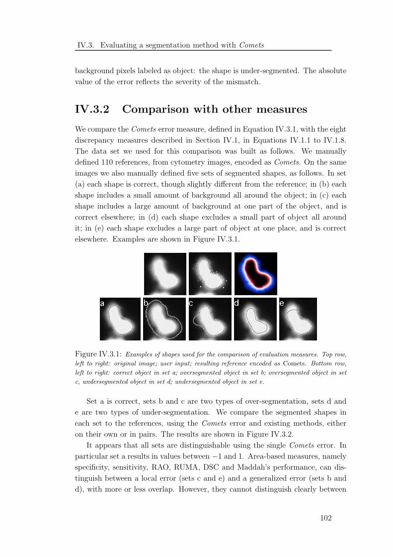
IV.3. Evaluating a segmentation method with Comets
background pixels labeled as object: the shape is under-segmented. The absolute
value of the error reflects the severity of the mismatch.
IV.3.2 Comparison with other measures
We compare the Comets error measure, defined in Equation IV.3.1, with the eight
discrepancy measures described in Section IV.1, in Equations IV.1.1 to IV.1.8.
The data set we used for this comparison was built as follows. We manually
defined 110 references, from cytometry images, encoded as Comets. On the same
images we also manually defined five sets of segmented shapes, as follows. In set
(a) each shape is correct, though slightly different from the reference; in (b) each
shape includes a small amount of background all around the object; in (c) each
shape includes a large amount of background at one part of the object, and is
correct elsewhere; in (d) each shape excludes a small part of object all around
it; in (e) each shape excludes a large part of object at one place, and is correct
elsewhere. Examples are shown in Figure IV.3.1.
Figure IV.3.1: Examples of shapes used for the comparison of evaluation measures. Top row,
left to right: original image; user input; resulting reference encoded as Comets. Bottom row,
left to right: correct object in set a; oversegmented object in set b; oversegmented object in set
c, undersegmented object in set d; undersegmented object in set e.
Set a is correct, sets b and c are two types of over-segmentation, sets d and
e are two types of under-segmentation. We compare the segmented shapes in
each set to the references, using the Comets error and existing methods, either
on their own or in pairs. The results are shown in Figure IV.3.2.
It appears that all sets are distinguishable using the single Comets error. In
particular set a results in values between −1 and 1. Area-based measures, namely
specificity, sensitivity, RAO, RUMA, DSC and Maddah’s performance, can dis-
tinguish between a local error (sets c and e) and a generalized error (sets b and
d), with more or less overlap. However, they cannot distinguish clearly between
102

IV.3. Evaluating a segmentation method with Comets
Figure IV.3.2: Results of the comparison of evaluation methods. All the values plotted are
defined in Equations IV.1.1 to IV.1.8 and IV.3.1. Top two rows: single evaluation measures.
Bottom two rows: pairs of evaluation measures. On these graphs only the Comets error measure
(on the top left) shows a clear separation of all five sets.
103

IV.3. Evaluating a segmentation method with Comets
under-segmentation (sets b and c) and over-segmentation (sets d and e). Con-
versely, Hausdorff-distance based measures can perform the opposite distinctions.
This prevents distinguishing between over- and under-segmentation. Also, even
though most results in set a are below all other sets, there is no threshold value
separating them. Yet, combining them may not be enough to distinguish all
cases. At least three of these discrepancy measures seem necessary, on this data
set, to separate clearly the five sets.
IV.3.3 Evaluation of a segmentation method
The measure defined in Equation IV.3.1 can be used to evaluate a segmentation
method, as follows. Let Ci1≤i≤n be the n references, and Sj1≤j≤m the m
segmented shapes returned by the method to evaluate. Let EM be the n × merror matrix defined as:
EM (i, j) = error(Sj, Ci) (IV.3.2)
Row i lists the errors of the method against reference Ci; if it is filled with∞, Ci
is missed. Similarly, column j shows the errors of the segmented shape Sj ; if it
is filled with ∞, Sj is noise.
As an illustration, the error matrix for the example in Figure IV.3.3 is:
EM =(error(Sj , Ci)
)i,j
=
0 ∞ ∞ ∞ ∞∞ 5 15 ∞ ∞∞ ∞ ∞ ∞ ∞
← C1
← C2
← C3
↑ ↑ ↑ ↑ ↑S1 S2 S3 S4 S5
(IV.3.3)
As explained in Section I.2.3, there is an inherent ambiguity when presenting
evaluation results. For clarification, we differentiate between a reference viewpoint
and a user viewpoint. From a reference viewpoint, what matters is to assess how
well each reference is segmented. The score obtained by reference Ci is the score
with the lowest absolute value in row i in the error matrix. Formally:
scoreRef (Ci) = EM (i, j0) where j0 = arg min1≤j≤m
|EM (i, j)| (IV.3.4)
C1 C2 C3 S1 S2 S3 S4 S5
Figure IV.3.3: Example of segmentation, to illustrate user and reference viewpoints. Left:
image with three references Ci. Right: same image with five segmented objects Sj.
104

IV.3. Evaluating a segmentation method with Comets
These n scores can be interpreted in terms of correct, under- and over-segmented,
and missed references, using the score sign and value as explained above. How-
ever, they do not account for the segmented objects classified as noise (columns
filled with ∞). To do so, we add the following scores (negative to distinguish
from missed references):
scoreRef (Sj) = −∞ if min1≤i≤n
EM (i, j) =∞ (IV.3.5)
As an example, consider Figure IV.3.3 and the error matrix in Equation IV.3.3.
The score of the segmentation method, from a reference point of view as defined
in Equations IV.3.4 and IV.3.5, is constructed as follows:
0 ∞ ∞ ∞ ∞∞ 5 15 ∞ ∞∞ ∞ ∞ ∞ ∞
empty ↓ ↓columns −∞ −∞
min
→ 0
→ 5
→ ∞
scoreRef = [ 0, 5, ∞, −∞, −∞ ]
Another way to interpret evaluation results, from a user viewpoint, is to assess
how well each segmented object fits a reference. It shows how many segmented
objects match a reference, or how many cause oversegmentation. The score ob-
tained by a segmented object Sj is the entry with the lowest absolute value in
column j of the error matrix, defined as:
scoreUser(Sj) = EM (i0, j) where i0 = arg min1≤i≤n
|EM (i, j)| (IV.3.6)
Again these m scores can be interpreted in terms of correct, under-, over-, and
noisy segmentated objects. Since they do not account for the missed references,
we add the following scores:
scoreUser(Ci) = −∞ if min1≤j≤m
EM (i, j) =∞ (IV.3.7)
Using Figure IV.3.3 and the error matrix in Equation IV.3.3, the score from a
user viewpoint defined in Equations IV.3.6 and IV.3.7, is constructed as:
min
0 ∞ ∞ ∞ ∞∞ 5 15 ∞ ∞∞ ∞ ∞ ∞ ∞↓ ↓ ↓ ↓ ↓0 5 15 ∞ ∞
empty
lines
→ −∞
scoreUser = [ 0, 5, 15, ∞, ∞, −∞ ]
and can be interpreted qualitatively as follows. From a reference viewpoint, one
reference is perfectly segmented, one is severely over-segmented, one is missed,
105
IV.3. Evaluating a segmentation method with Comets
and two non-existing object are segmented. From a user viewpoint, one segmented
object fits exactly a reference, two severely oversegment references, two are noise,
and one reference is missed. In practice, error matrices are very sparse, and only
require storing in the order of n entries.
IV.3.4 Tuning of a segmentation method
In this section we illustrate how the evaluation method presented above can be
used to tune a segmentation method’s parameters based on a large number of
references. We use our nucleic segmentation method, presented in Chapter III.
In a first round of experiments, we tune the proportion values used to initialise
the EM algorithm, as listed in Table IV.3.1. In a second round, we tune the total
number of iterations of the EM algorithm. Finally, in a third round of experiments
we tune the maximum number of components allowed in the EM algorithm. More
details on these parameters are provided in Section III.1.2 page 66.
We defined 250 Comets references, as detailed above, on a subset of images,
and use these objects to tune the parameters. For each round of experiments,
we choose a set of parameter values as a control and perform the segmentation.
We measure the Comets error for each reference i, and note it scoreRef (Cctri ).
We then choose a set s of parameters values, and segment the reference images
again. For each reference i the Comets error (from a reference viewpoint) is noted
scoreRef (Csi ). For each reference i we then compute the ratio:
ρsi =
scoreRef (Csi )
scoreRef (Cctri )
(IV.3.8)
These ratios can be interpreted in the following way:
|ρsi | ≤ 0.5 : the segmentation is better with parameter values s
0.5 < |ρsi | ≤ 1.5 : the segmentation is similar to the control
|ρsi | > 1.5 : the segmentation is worse with parameter values s
The threshold values 0.5 and 1.5 are somewhat arbitrary; the whole plots of ρsi
values are available for comparison.
The parameter values used in our experiments are listed in Tables IV.3.2,
IV.3.3 and IV.3.4. The results are presented in Figure IV.3.4.
The first round of experiments show that with the parameters in Set 5, the
proportion of nuclei having a worse segmentation is the lowest, while the pro-
portion of nuclei having a better segmentation is the highest. We keep these
values for the rest of the experiments, as a control for the second round. In that
round, with the parameters used in Set 11, the proportion of nuclei with a better
106
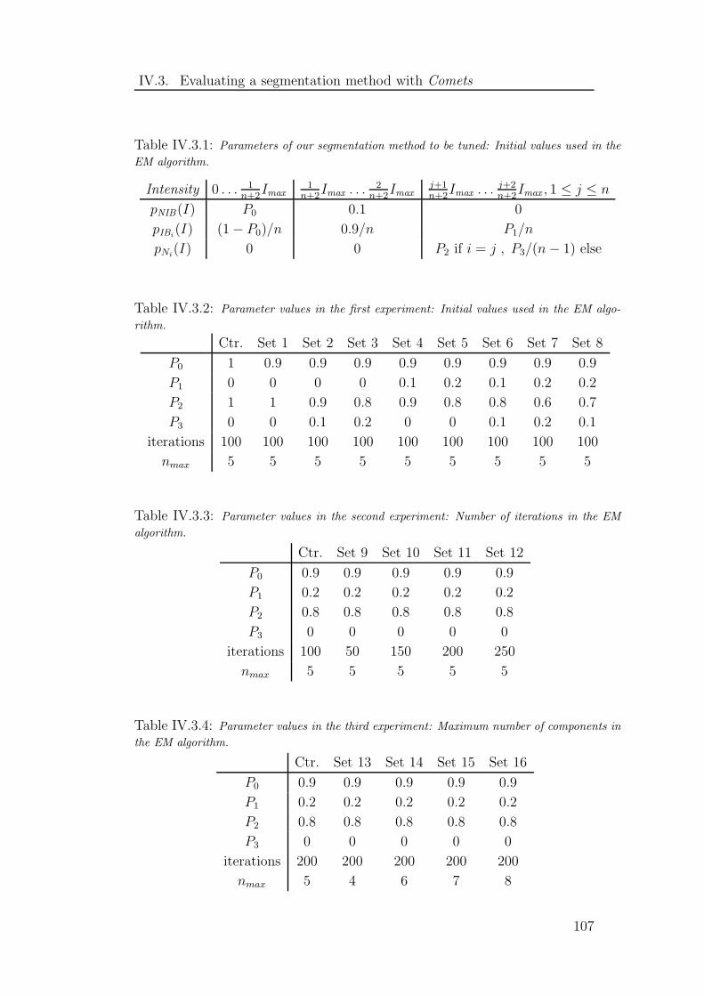
IV.3. Evaluating a segmentation method with Comets
Table IV.3.1: Parameters of our segmentation method to be tuned: Initial values used in the
EM algorithm.
Intensity 0 . . . 1n+2
Imax1
n+2Imax . . .
2n+2
Imaxj+1n+2
Imax . . .j+2n+2
Imax , 1 ≤ j ≤ n
pNIB(I) P0 0.1 0
pIBi(I) (1− P0)/n 0.9/n P1/n
pNi(I) 0 0 P2 if i = j , P3/(n− 1) else
Table IV.3.2: Parameter values in the first experiment: Initial values used in the EM algo-
rithm.
Ctr. Set 1 Set 2 Set 3 Set 4 Set 5 Set 6 Set 7 Set 8
P0 1 0.9 0.9 0.9 0.9 0.9 0.9 0.9 0.9
P1 0 0 0 0 0.1 0.2 0.1 0.2 0.2
P2 1 1 0.9 0.8 0.9 0.8 0.8 0.6 0.7
P3 0 0 0.1 0.2 0 0 0.1 0.2 0.1
iterations 100 100 100 100 100 100 100 100 100
nmax 5 5 5 5 5 5 5 5 5
Table IV.3.3: Parameter values in the second experiment: Number of iterations in the EM
algorithm.
Ctr. Set 9 Set 10 Set 11 Set 12
P0 0.9 0.9 0.9 0.9 0.9
P1 0.2 0.2 0.2 0.2 0.2
P2 0.8 0.8 0.8 0.8 0.8
P3 0 0 0 0 0
iterations 100 50 150 200 250
nmax 5 5 5 5 5
Table IV.3.4: Parameter values in the third experiment: Maximum number of components in
the EM algorithm.
Ctr. Set 13 Set 14 Set 15 Set 16
P0 0.9 0.9 0.9 0.9 0.9
P1 0.2 0.2 0.2 0.2 0.2
P2 0.8 0.8 0.8 0.8 0.8
P3 0 0 0 0 0
iterations 200 200 200 200 200
nmax 5 4 6 7 8
107

IV.3. Evaluating a segmentation method with Comets
Set 1 Set 2 Set 3 Set 4
worse 30.67% 38.84% 37.30% 33.57%
same 29.47% 21.39% 20.37% 24.04%
better 39.86% 39.77% 42.33% 42.39%
Set 5 Set 6 Set 7 Set 8
worse 26.12% 37.87% 41.32% 38.81%
same 24.06% 21.69% 20.84% 20.15%
better 49.82% 40.44% 37.84% 41.04%
Set 9 Set 10 Set 11 Set 12
worse 41.21% 34.60% 33.38% 33.33%
same 20.17% 23.93% 23.27% 25.34%
better 38.62% 41.47% 43.35% 41.32%
Set 13 Set 14 Set 15 Set 16
worse 47.66% 41.35% 43.78% 49.45%
same 16.15% 22.76% 22.65% 20.75%
better 36.19% 35.89% 35.57% 29.80%
Figure IV.3.4: Results of the three experiments on parameter tuning. Top row: first experi-
ments. Bottom row, left: second experiment; right: third experiment. The graphs show on the y
axis the proportion of nuclei having the ratio values on the x axis, as defined in Equation IV.3.8.
The tables list the proportions of nuclei for which the set parameters induce a worse, similar or
better segmentation than with the control parameters.
Figure IV.3.5: Evaluation results of our nucleic segmentation and the watershed with the
Comets measure. The graphs show on the y axis the proportion of references having a score
value on the x axis.
108

IV.3. Evaluating a segmentation method with Comets
segmentation than the control is the highest, while the proportion of nuclei with
a worse segmentation is almost the lowest (33.38% against 33.33% for Set 12).
We keep Set 11 for the rest of the experiments. In the third round however, with
all parameter values the proportion of nuclei with a worse segmentation is higher
than that with a better segmentation. We conclude that none of the parameter
values outperform the control chosen, and thus keep the control (Set 11) as the
best set of values. These values are similar to the actual values chosen by visual
evaluation of the results in Chapter III.
The Comets scores for Set 11 are shown in Figure IV.3.5, along with the scores
of the watershed-based segmentation, presented in Chapter III, for comparison.
The two peaks on the red curve show that most of the nuclei segmented with
our method score either close to 1 or −1, while the single peak in values above 1
on the blue curve indicate that most nuclei tend to be over-segmented with the
watershed.
The proportion of references with a score between -1 and 1 is 68.4% with Set
11 parameters, and 36.4% with the watershed. Using a range between −2 and 2,
these proportions are respectively 77.1% and 68.4%. Although our method still
outperforms the watershed, these values are significantly lower than those found
by visual evaluation of the results, in Chapter III. A first explanation is that the
subset of images chosen for this automatic evaluation are from only two individu-
als, and may not be representative enough of the diversity of images. Our future
work includes marking more references from all individuals. A second explana-
tion is that a visual inspection of segmentation results may be more lenient than
a strict comparison with fixed references.
Even though these final proportions may be not representative enough, the
methodology presented here allows a systematic tuning of parameters and a com-
parison of different segmentation methods, using a large number of objects.
109
Summary
We have presented our novel model, Comets, a single framework that allows:
- The encoding of segmentation references with local confidence factors, stor-
ing more expert knowledge than a single shape at a low cost;
- The combination of multiple references, with confidence-based local weights;
- A single discrepancy measure that allows an easy interpretation of seg-
mentation results, in qualitative (correct, under-, over-segmented, missed,
noise) and quantitative (severity) terms.
To the best of our knowledge, existing methods can perform only one of the
above. These actions are based on local confidence factors, which are automat-
ically computed from an expert user’s input. The extra input needed, namely
the limit pixels, is less demanding that landmark selection, and can easily be
added to existing systems. All the information used in our model is provided by
human experts. In particular no parameter is used, and no assumption is made
to combine multiple shapes, unlike existing methods as [185]. This makes our
model independent of segmentation methods, as defined in [91]. We have pre-
sented results of discrepancy measures, showing that the Comets error is more
conclusive than some commonly used metrics.
This framework can be used to compare qualitatively and quantitatively dif-
ferent segmentation methods applied to the same set of images. In particular, it
can be used to tune the parameters of a segmentation method. Since such com-
parisons may be ambiguous, we have presented two different ways to evaluate a
segmentation method: from a reference and from a user viewpoint.
Discrepancy evaluation has been little used according to Zhang [201], who
concludes by calling for “new ideas and procedures for the methodology and
practical implementation of evaluation”. We have presented here a novel method
for discrepancy evaluation and detailed its implementation.
110

Chapter V
Discussion and Future Work
111

This chapter draws together the points made throughout this work. It dis-
cusses what contributions have been made, their strengths and possible improve-
ments, and presents possible future projects connected to this work. Since our
project has been application-driven, there are two complementary aspects to the
discussion and contributions: from a computer vision point of view, and from a
cytometry point of view. We start with computer vision, where we discuss our
novel segmentation methods and our novel evaluation framework, and present
some possible extensions of this framework and its uses. We then discuss the
cytometric application of our work, within the SAFE Network of Excellence, and
draw some conclusions from the pilot study we conducted. We also present some
future projects aimed to improve the detection of fetal cells within maternal cir-
culation.
112

V.1. Computer Vision
Our work has made contributions in two fields of computer vision: segmentation
and evaluation.
Our nucleic segmentation method consists in modeling the image formation,
in order to derive a model of image histogram. That model is then fitted to actual
data by an adapted Expectation-Maximisation algorithm. When fitted, the model
allows the selection of relevant threshold values, first global then local, which are
used to segment the nuclei in the images. The image model that we developed
is meant to evaluate the impact of object fluorescence in the surrounding back-
ground regions. The thresholds used to segment out the background are directly
derived from the model we developed for this type of image formation. As a re-
sult, they have a strong theoretical justification, as opposed to other thresholding
methods based non-realistic assumptions on histogram shapes. This approach to
segmentation consists in gradually ruling out the background, until the objects
of interest are correctly segmented. It differs from most existing segmentation
methods, in which the objects are gradually ruled in (such as watershed or active
contours). Our approach is more robust in our context, where the background is
more predictable and easy to model than the objects. However, it is not able to
isolate touching objects: this is why an extra step was needed in our segmenta-
tion method, based on an inner threshold which has no theoretical foundations.
The issue of segmenting touching non-convex nuclei in 2D microscopy is generally
acknowledged as challenging, not the least because even human experts cannot
always perform it reliably. Our method is based on a simple observation: human
experts can isolate touching nuclei when a dark path connects different sides of
their borders. This can be seamlessly integrated to our segmentation method, as
presented in Chapter III. However, it is difficult to evaluate this step alone, since
no ground truth can be relied on. As a comment on our model, the particular pro-
file chosen – a decreasing exponential – was not derived from a theoretic model.
We believe that too many unknown factors contribute to the side illumination to
113
V.1. Computer Vision
model it completely. In particular, the density and constitution of the materials
surrounding the nuclei in the slide, and the volumetric geometry of the nuclei
would need to play a significant role in such a model, while very little is know on
them. Any other decreasing function may be tested, such as inverse quadratic,
by simply ‘plugging’ it into the equations, to derive new illuminated background
functions, and new formulas to compute their parameters from a weighted his-
togram. By this we mean that our segmentation method, while using a specific
profile, is not dependent on it, and could be tested with other ones.
The Expectation-Maximisation (EM) algorithm is in fact, in its general form,
a class of algorithms meant to fit a parametric model to incomplete data, through
an iterative process. The particular algorithm we presented in Chapter III is
adapted to histogram modeling. EM algorithms have two notorious weaknesses:
first, their can be very sensitive to the initialisation chosen for the iterative pro-
cess. Second, the more components are added to the model, the better the fit
tend to be. In our case, the initialisation consists in choosing the proportions of
each component over the histogram range of values. These values are somewhat
constrained by the nature of the model: the non-illuminated background func-
tion will always model the darker pixels, the nuclei function will always model
the brighter pixels, and the illuminated background function will model most
of the pixels in-between. We have conducted a series of experiments where we
vary the proportions, in keeping with these qualitative constraints, detailed in
Chapter IV. The search for better parameters is still an open question: as there
is no theoretical justification of the initial values in our context, we use these
empirically found values. Regarding the second issue, our method actually does
not suffer from it. Increasing the number of components (i.e. the value of n in
our model) does not always improve the error, as illustrated by the last round
of experiments in Chapter IV. This is because the components of our model are
not independent, unlike in other models such as mixtures of Gaussians. In our
model, each type a component is added, two new functions are included: one for
the nuclei (an extra function Ni) and one for the illuminated background (an ex-
tra function IB i). Each illuminated background function models a high number
of pixels of low intensity: adding one such function, even with a low weight, has
a significant impact on the model at the low intensities. As a result, having too
many of these functions will significantly raise the distance between the model
and the data. While the main issues of EM algorithms have no significant impact
in our context, open questions remain on the choice of parameter values: the
initial values of the model, the total number of iterations used, and the error
measure chosen, have an impact on the final model chosen, but are only chosen
through prior experiments.
114

V.1. Computer Vision
Our probe segmentation method is meant to avoid segmenting foreground
noise (i.e. unwashed and unattached fluorescent probes), which is the most se-
vere issue in our context. Bearing in mind that nuclei overlapped by foreground
noise occur much more frequently (by a few orders of magnitude) than fetal nu-
clei within maternal circulation, it is important to avoid classifying one for the
other. By segmenting out foreground noise, our method ensures that it does not
affect the measures of fluorescence in nuclei. A second important point is the
number of probes visible within nuclei. As detailed in Chapter III, this number is
a rough estimation of the imaging quality of a sample. Nuclei showing less than
twenty probes are either affected by blur, foreground noise overlap, or low probe
attachment rate. By segmenting probes of a given size, our method can directly
evaluate the number of probes within each nuclei, while other methods cannot
(such as top-hat transform). These two properties of our probe segmentation
method are important when it comes to drawing conclusions from the pilot study
conducted as a SAFE project.
Our two methods of segmentation have success rates of over 99% on our data
set, containing nearly 14,000 nuclei. This is a significant improvement over ex-
isting methods, especially for nucleic segmentation, where typical success rates
are about 80%. However, it is important to bear in mind that in most exist-
ing cytometric applications, a success rate of 80% is already more than enough.
Some applications require the segmentation of a fixed number of nuclei, e.g. 200,
or a proportion of nuclei below 80%. We think this is why existing segmenta-
tion methods have not been pushed towards better results, which often come at
the cost of lower robustness to imaging conditions, and why simple segmentation
methods such as low-level vision, watershed or active contours are still commonly
used in cytometry, when they are now obsolete in other applications of computer
vision. In our context however, higher rates where required, for both nuclei and
probes, with no alteration to robustness or automation.
While success rates are intuitive to interpret, we wish to emphasis that evalu-
ating segmentation methods is a challenging issue, especially on images showing
multiple objects. It can be argued that segmentation is a form of classification,
which leads to using the frameworks of classifiers evaluations, such as Receiver-
Operating Characteristic (ROC) curves. Classification outcomes are usually clas-
sified in four categories, namely true and false positive and negative. However,
when it comes to segmenting objects, it can be difficult to use such categories.
Using them on a pixel basis leads to evaluation results that are challenging to
interpret. On the other hand, using them on a full object basis leads to pes-
simistically biased results: even when a segmentation is correct, it very rarely
matches a reference perfectly. Secondly, we consider that using four categories
115

V.1. Computer Vision
of results does not always give enough insight into segmentation methods. Over-
segmented and under-segmented objects would fall in the same category, as would
minor and severe errors. In our context, these different types of errors are not
equivalent, and the severity of mis-segmentation is important. For these reasons,
in Chapter III we presented results using five categories, and in Chapter IV we
introduced a method to measure the severity of errors at the same time.
The novel framework for discrepancy evaluation introduced in Chapter IV,
called Comets, is meant to provide results with a direct and simple interpreta-
tion, even for objects affected by blur and ambiguity. It was designed so that the
measure between a segmented object and a reference would reflect both the type
of difference between them (over or under-segmentation), and its severity, with
a single real number. By convention, a number between -1 and 1 is interpreted
as a correct result, with 0 being a perfect match with the reference. A number
below -1 reflects under-segmentation, and a number above 1, over-segmentation.
In both cases, the higher absolute value of the number, the more severe the error.
This is achieved by encoding the references as confidence maps, and not only
binary masks or sharp boundaries as is often the case. A confidence map assigns
each pixel in and around an object a number, which reflects the user’s confidence
that the pixel belongs to the background, the object, or the boundary. The higher
the confidence assigned to a pixel, the more severe a mislabeling of this pixel is.
Based on this observation, the error between a segmented object and a reference
can simply be defined as the confidence of a mislabeled pixel with the maximum
absolute value. As detailed in Chapter IV, such a confidence map can be defined
manually by a user through simple clicks, and encoded as a text file in an efficient
way. One of the strengths of this approach is that the confidence maps may look
different in various parts of the object, depending on the local level of blur, or the
presence of nearby objects. However, segmented objects often suffer from both
under- and over-segmentation. Since the error measure we introduced consists of
only one number, only the worst of these two errors is kept for the evaluation.
When they are of similar severity, the final outcome may be somehow arbitrary;
and when the parameters of a segmentation methods are slightly changed, an ob-
ject may suddenly have an error with a different sign. This issue may be avoided
by defining the error as a couple of real numbers: the lowest negative and the
highest positive confidence of mislabeled pixels. It would still make the results
intuitive to interpret, though possibly less easy to visualise and compare. Other
possible extensions of the Comets framework include defining confidence maps
for 3D data, and exploring its uses in non-medical data.
Along with the error measure developed, we clarified in Chapter IV the defi-
nition of success rates for images showing multiple objects. First, each object can
116

V.1. Computer Vision
be measured against each reference. Then, from a reference point of view, the best
scores achieved on each reference are kept, along with the number of objects not
matching any reference. Conversely, from a user point of view, the best scores
achieved by each object are kept, along with the number of missed references.
Both approaches can be interpreted in their own right, to define rates of success,
over-segmentation, etc. Using the reference point of view, this framework allows
a systematic evaluation of a segmentation method on a potentially large set of
data, quickly and automatically. We illustrated this in Chapter IV, and showed
that it can be used to tune the parameters of a segmentation method, or to com-
pare different methods. However, it requires the prior definition of references as
confidence maps in the Comets framework.
117

V.2. Cytometry
As detailed in Chapter I, this work is part of the SAFE Network of Excellence,
and our particular interest lies in the search for markers to discriminate fetal from
maternal nuclei within maternal circulation. The particular marker tested in this
work is the fluorescence of telomeric probes, as an indication of the telomeric
length, known to be higher in fetal nuclei than in maternal ones. To assess this
marker and its potential to discriminate, a pilot study was conducted, by some
of the SAFE partners, involving a series of blind tests. For each test, a sample of
fetal cells, along with one or two samples from adults, were processed separately
but in the same way, resulting in a series of fluorescence microscopy images from
each individual. These images were anonymised and processed by the software
we developed, which implemented the segmentation methods and measures de-
tailed in Chapter III. The goal of this pilot study was to evaluate whether the
protocols and measures used (from the cell preparation to the imaging and the
image processing) resulted in a clear separation of the fetal nuclei from the adult
ones.
The results we obtained are presented and discussed in Chapter III. At this
stage, the conclusions to be drawn from this pilot study belong to the SAFE Net-
work of Excellence, and several partners are involved. They are far beyond the
scope of this work, which is why we do not include them here. We only discuss
some implications of our results.
The main observation from the results on the blind trials is that in each case,
one individual stands out as having brighter probes. This tends to show that the
method used can efficiently distinguish different un-mixed populations of nuclei
based on their telomeric length. However useful as it may be, this is significantly
different from an original goal of this work, which required to isolate a few nuclei
within another population based on their telomeric length. The results obtained
during the pilot test show that the overlap between the populations is still too
large to distinguish between individuals of different populations with certainty.
118

V.2. Cytometry
Improving the segmentation results beyond 99.3% would not be enough to reduce
the overlap, but other improvements are likely to have an effect on it.
The results presented in Chapter III also show that in two blind trials, the
number of probes visible per nuclei are below the expected values. This suggests
that either the probe attachment rate during the biological processing of the sam-
ple, or the imaging quality of the microscopic hardware used were not optimal.
It appears that in the two cases, images were affected by visual and motion blur.
This implies that the imaging quality could be improved, and at present the mea-
sures performed on the two blind trials concerned are not as conclusive as they
could be.
At this stage, we are only in a position to call for improved imaging quality
in the future pilot studies. Although the first results obtained show that telom-
eric probe fluorescence can be used to distinguish populations of nuclei but not
individual nuclei yet, more tests with higher imaging quality are needed before
definite conclusions on this marker can be drawn.
In the next section we present future projects, the first of which could also be
used to increase the conclusiveness of the measures.
119
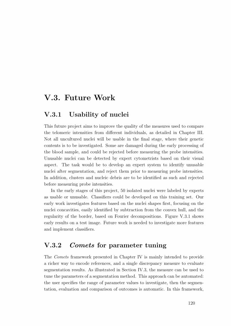
V.3. Future Work
V.3.1 Usability of nuclei
This future project aims to improve the quality of the measures used to compare
the telomeric intensities from different individuals, as detailed in Chapter III.
Not all uncultured nuclei will be usable in the final stage, where their genetic
contents is to be investigated. Some are damaged during the early processing of
the blood sample, and could be rejected before measuring the probe intensities.
Unusable nuclei can be detected by expert cytometrists based on their visual
aspect. The task would be to develop an expert system to identify unusable
nuclei after segmentation, and reject them prior to measuring probe intensities.
In addition, clusters and nucleic debris are to be identified as such and rejected
before measuring probe intensities.
In the early stages of this project, 50 isolated nuclei were labeled by experts
as usable or unusable. Classifiers could be developed on this training set. Our
early work investigates features based on the nuclei shapes first, focusing on the
nuclei concavities, easily identified by subtraction from the convex hull, and the
regularity of the border, based on Fourier decompositions. Figure V.3.1 shows
early results on a test image. Future work is needed to investigate more features
and implement classifiers.
V.3.2 Comets for parameter tuning
The Comets framework presented in Chapter IV is mainly intended to provide
a richer way to encode references, and a single discrepancy measure to evaluate
segmentation results. As illustrated in Section IV.3, the measure can be used to
tune the parameters of a segmentation method. This approach can be automated:
the user specifies the range of parameter values to investigate, then the segmen-
tation, evaluation and comparison of outcomes is automatic. In this framework,
120
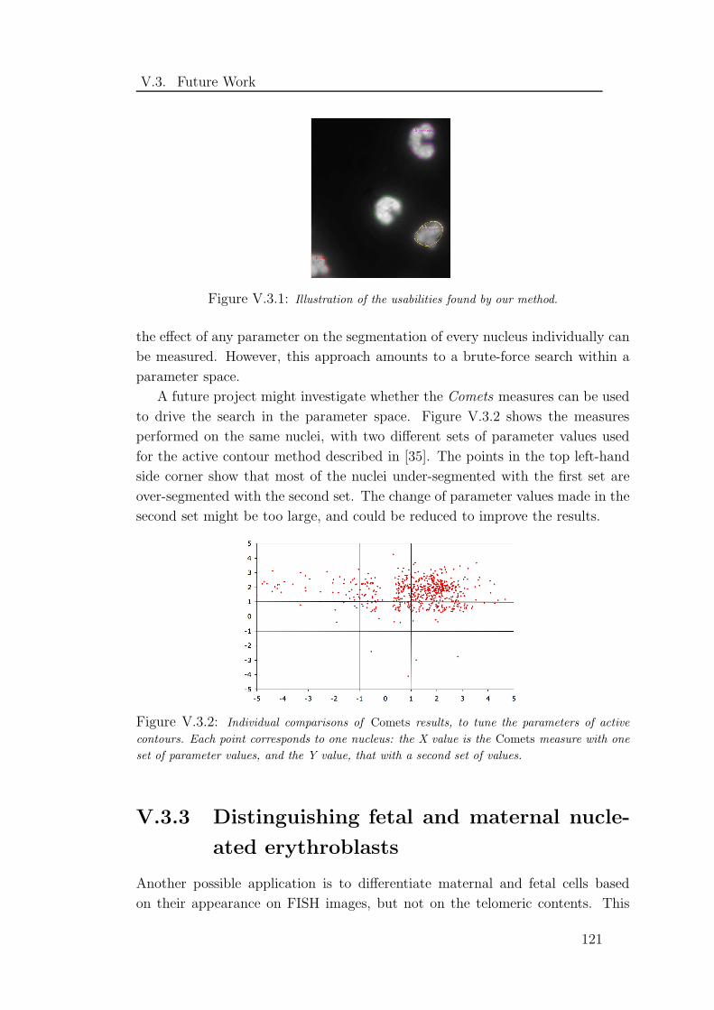
V.3. Future Work
Figure V.3.1: Illustration of the usabilities found by our method.
the effect of any parameter on the segmentation of every nucleus individually can
be measured. However, this approach amounts to a brute-force search within a
parameter space.
A future project might investigate whether the Comets measures can be used
to drive the search in the parameter space. Figure V.3.2 shows the measures
performed on the same nuclei, with two different sets of parameter values used
for the active contour method described in [35]. The points in the top left-hand
side corner show that most of the nuclei under-segmented with the first set are
over-segmented with the second set. The change of parameter values made in the
second set might be too large, and could be reduced to improve the results.
Figure V.3.2: Individual comparisons of Comets results, to tune the parameters of active
contours. Each point corresponds to one nucleus: the X value is the Comets measure with one
set of parameter values, and the Y value, that with a second set of values.
V.3.3 Distinguishing fetal and maternal nucle-
ated erythroblasts
Another possible application is to differentiate maternal and fetal cells based
on their appearance on FISH images, but not on the telomeric contents. This
121

V.3. Future Work
project would focus on nucleated erythroblasts, or red-blood cells. Erythroblasts
are mostly free of nuclei, except fetal erythroblasts in maternal blood, and a few
maternal ones. They can be distinguished visually by expert cytologists. The
project would develop an expert system to reproduce this distinction.
An early training set contains 230 examples of nucleated erythroblasts, man-
ually marked as fetal or maternal, as illustrated on the left of Figure V.3.3. Our
segmentation method can be used to segment the nuclei, in blue, as illustrated
on the right of Figure V.3.3. However it cannot be used directly for the segmen-
tation of the cytoplasm, in green. When cells are close and overlap, the green
intensity at the border can be higher than within the cells. Our method to sep-
arate touching objects requires a darker region between them, and will fail on
some images. It would be necessary to adapt it to the visual properties of red
blood cells, then develop a classifier to distinguish between maternal and fetal
nucleated erythroblasts.
Figure V.3.3: Nucleated erythroblasts. Left: fetal one, marked in red, and maternal one,
marked in blue. Right: results of our nucleic segmentation method.
122
V.4. Conclusion
In this dissertation we have presented our contributions to the automation of cell
image analysis, in particular the segmentation of fluorescent nuclei and probes,
and the evaluation of segmentation results. We have developed two novel seg-
mentation methods, adapted for nuclei and probes in Fluorescence in-situ Hy-
bridisation images. We have demonstrated that they are both robust, automated,
and achieve 99.3% accuracy on our database of over two thousand images. We
have compared them with state-of-the-art techniques used in cytometry, which
we reviewed in detail, and discussed their strengths. We have used them to show
that telomeric probe intensities are a promising approach to distinguish between
maternal and fetal uncultured leucocytes, and shown that imaging quality is a
key factor to improve the distinction.
We have also presented Comets, a novel framework for discrepancy evaluation
of segmentation methods, in the context of medical imaging. This framework
allows the encoding of expert segmentation references with local confidence fac-
tors, can be used to combine multiple references of objects, and provides a single
measure that can be easily interpreted quantitatively and qualitatively. We have
shown that this measure can be used to tune a segmentation method’s parameters
on a large volume of data.
In the Appendices we have detailed the implementation of our methods on
a distributed computing environment. We have presented the XML database
structures adapted to the storage of references and different results, and the
architecture and protocols used to achieve a reliable, scalable and robust process-
ing of large number of images, and the main graphical user interfaces. We have
presented quantitative results showing the performance of our program on this
distributed environment.
We hope that our work will contribute to the success of the European Commis-
sion-funded Network of Excellence SAFE, and through it to the progress of cy-
tometry and prenatal genetic disease detection.
123

Related publications
The following papers, published or under review, are related to the contents of
this dissertation.
- Christophe Restif and William F. Clocksin. Comparison of segmentation
methods for cytometric assay. In Medical Image Understanding and Anal-
ysis, pages 153-156, London, UK, September 2004.
- Christophe Restif. Towards Safer, Faster Prenatal Genetic Tests: Novel
Unsupervised, Automatic and Robust Methods of Segmentation of Nuclei
and Probes. In European Conference on Computer Vision, pages 437-450,
Graz, Austria, May 2006.
- Anthony J. McCollum, Christophe Restif and William F. Clocksin. Imaging
system design for detecting small changes in telomere length. In Medical
Image Understanding and Analysis, pages 206-210, Manchester, UK, July
2006.
- Christophe Restif, William F. Clocksin. Computer Vision for Segmentation
in Cytometry. Submitted to ACM Computing Surveys in December 2005.
124

Appendices
125

A. Algorithms
A.1 Low-level vision algorithms
Grayscale reconstruction
This operation is based on conditional dilation. Let m be a mask, i.e. an image
with the same dimensions as f but a different content. The condition dilation of
f by kernel k under the mask m is:
f ⊕m k = (f ⊕ k) ∧m (A.1)
where ∧ is the pixel-wise minimum operator, defined as:
(f1 ∧ f2)(x, y) = min(f1(x, y), f2(x, y)) (A.2)
Conditional dilations are iterated as:
(f ⊕m k)n+1 = (f ⊕m k)n ⊕m k , n ≥ 1 (A.3)
Since this sequence is increasing and has discrete and bounded (grayscale) values,
conditional dilations converge after a finite number of iterations. The resulting
image is the grayscale reconstruction of image f under mask m with kernel k,
and is noted:
f ⊥k m = (f ⊕m k)∞ (A.4)
To extract domes of high h (in gray values), the image to reconstruct is f−h,
defined as f−h(x, y) = max(0, f(x, y) − h). In the reconstruction of f−h under
the mask f , the domes are actually cut off. Thus, the domes of high h are the
connected components of the image gdome defined as:
gdome = f − (f−h ⊥kdomef) , kdome =
0 0 0
0 0 0
0 0 0
(A.5)
126

Appendix A. Algorithms
Gradient Vector Flow
The GVF is defined as the field g(x, y) = (gx(x, y), gy(x, y)) which minimises the
energy functional:
ε =∑
x,y
µ |∇g|2(x, y) + ‖∇f(x, y)‖2 · ‖g(x, y)−∇f(x, y)‖2 (A.6)
where |∇g|2 =
(∂gx
∂x
)2
+
(∂gx
∂y
)2
+
(∂gy
∂x
)2
+
(∂gy
∂y
)2
(A.7)
and µ is a constant, weighting the relative importance of smoothing g: the noisier
the image f , the higher µ should be [194]. The functional ε can be minimised by
an iterative process, using finite differences in space (steps δx and δy) and time
(step δt). Using the following notations from [195]:
∂xf(x, y) = f(x+ 1, y)− f(x, y) , cx(x, y) = b(x, y) · ∂xf(x, y)
∂yf(x, y) = f(x, y + 1)− f(x, y) , cy(x, y) = b(x, y) · ∂yf(x, y)
b(x, y) = (∂xf(x, y))2 + (∂yf(x, y))2 , r = µ · δt/(δx · δy)(A.8)
where r ≤ 4 to avoid oscillations, gx and gy are evaluated iteratively until con-
vergence, with the formulas:g0
x(x, y) = ∂xf(x, y)
gt+1x (x, y) = (1− b(x, y)δt) gt
x(x, y) + r∇2gtx(x, y) + cx(x, y)δt
(A.9)
where ∇2gtx(x, y) is the non-directional Laplacian of gt
x, defined above. gy is
computed with similar formulas, replacing the underscripts x with y. In [193],
Xu et al. suggest a more general energy functional defining GVF:
ε =∑
image
φ (‖∇f‖) |∇g|2 + ψ (‖∇f‖) ‖g −∇f‖2 (A.10)
and apply it with φ(r) = 1−e−( rκ)
2
, ψ(r) = e−( rκ)
2
, for a constant κ. The previous
definition of the GVF corresponds to the special case φ(r) = µ and ψ(r) = r2.
Chamfer distance transform
Supposing the foreground pixels are 1 and the background 0, the Chamfer algo-
rithm offers a quick way to compute the distance transform g of f by performing
only three scans of images, but requires one temporary image h. Initially, g and
h are two copies of f . First, g is filtered in the left-to-right top-down direction
with the filter kforward and the formula
g(x, y) = minkforward (i,j)>0
(kforward (i, j) + g(x+ i, y + j)) (A.11)
127
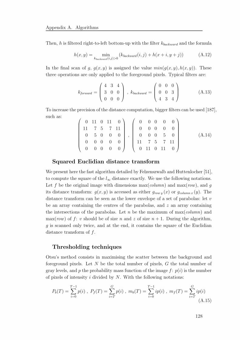
Appendix A. Algorithms
Then, h is filtered right-to-left bottom-up with the filter kbackward and the formula
h(x, y) = minkbackward (i,j)>0
(kbackward (i, j) + h(x+ i, y + j)) (A.12)
In the final scan of g, g(x, y) is assigned the value min(g(x, y), h(x, y)). These
three operations are only applied to the foreground pixels. Typical filters are:
kforward =
4 3 4
3 0 0
0 0 0
, kbackward =
0 0 0
0 0 3
4 3 4
(A.13)
To increase the precision of the distance computation, bigger filters can be used [187],
such as:
0 11 0 11 0
11 7 5 7 11
0 5 0 0 0
0 0 0 0 0
0 0 0 0 0
,
0 0 0 0 0
0 0 0 0 0
0 0 0 5 0
11 7 5 7 11
0 11 0 11 0
(A.14)
Squared Euclidian distance transform
We present here the fast algorithm detailed by Felzenszwalb and Huttenlocher [51],
to compute the square of the l∞ distance exactly. We use the following notations.
Let f be the original image with dimensions max(column) and max(row), and g
its distance transform: g(x, y) is accessed as either grow y (x) or gcolumn x (y). The
distance transform can be seen as the lower envelope of a set of parabolas: let v
be an array containing the centres of the parabolas, and z an array containing
the intersections of the parabolas. Let n be the maximum of max(column) and
max(row) of f : v should be of size n and z of size n + 1. During the algorithm,
g is scanned only twice, and at the end, it contains the square of the Euclidian
distance transform of f .
Thresholding techniques
Otsu’s method consists in maximising the scatter between the background and
foreground pixels. Let N be the total number of pixels, G the total number of
gray levels, and p the probability mass function of the image f : p(i) is the number
of pixels of intensity i divided by N . With the following notations:
Pb(T ) =T−1∑
i=0
p(i) , Pf(T ) =G∑
i=T
p(i) , mb(T ) =T−1∑
i=0
ip(i) , mf (T ) =G∑
i=T
ip(i)
(A.15)
128

Appendix A. Algorithms
Algorithm 3 Squared Euclidian Distance Transform
1: for i = 0 to max(column) do
2: for j = 0 to max(row) do
3: gcolumn i (j)← f(i, j) /* same as: grow j (i)← f(i, j) */
4: end for
5: end for
6: for coord = column , row do
7: for i = 0 to max(coord) do
8: k ← 0
9: v[0]← 0
10: z[0]← −∞11: z[1]← +∞
/* Compute the lower envelope of parabolas */
12: for q = 1 to n− 1 do
13: s← ((gcoord i (q) + q2)− (gcoord i (v[k]) + v[k]2)) /(2q − 2v[k])
14: while s ≤ z[k] do
15: k ← k − 1
16: s← ((gcoord i (q) + q2)− (gcoord i (v[k]) + v[k]2)) /(2q − 2v[k])
17: end while
18: k ← k + 1
19: v[k]← q
20: z[k]← s
21: z[k + 1]← +∞22: end for
/* Fill in the values of the distance transform */
23: k ← 0
24: for q = 0 to n− 1 do
25: while z[k + 1] < q do
26: k ← k + 1
27: end while
28: gcoord i (q)← (q − v[k])2 + gcoord i (v[k])
29: end for
30: end for
31: end for
129

Appendix A. Algorithms
Otsu’s threshold is defined as:
TOtsu = arg max0≤T≤G
Pb(T ) · Pf(T ) · [mb(T )−mf(T )]2
Pb(T ) · σ2b (T ) + Pf(T ) · σ2
f (T )(A.16)
where σ2b (T ) and σ2
f (T ) are the variances of the background and foreground pixels.
The isodata threshold Tiso is the value T for which the mean values of the
background pixels µb(T ) and foreground pixels µf (T ) are equidistant to T . It can
easily be computed iteratively:
T0 =G
2, Tn+1 =
µb(Tn) + µf(Tn)
2for n ≥ 0 (A.17)
stopping when the difference between Tn and Tn+1 is small enough (e.g. less than
1).
A.2 Watershed algorithm
We present here a popular algorithm to compute the watershed, published by Vin-
cent and Soille [180], and analysed by Roerdink and Meijster [144]. We adapted
it to use arbitrary markers as starting points for the immersion. In keeping with
our previous notations, let f be the original image and g the watershed trans-
form of f . Let dist be a helper image of the same size as f . Each pixel p has
an original value f(p), ranging from hmin to hmax, a label g(p), and a distance
dist(p) – initially 0. The possible label values g(p) are integers, with the following
conventions:
mask = −2 is a temporary value
init = −1 is the initial value of all pixels in g
wsh = 0 is the label of pixels in watershed lines
1, 2, 3, ... are the labels of the catchment basins
Let Marker be the set of the pixel marked as starting points for the flooding
process. Let fifo be a queue of pixels (a first-in-first-out data structure storing
pixels) with the following operations:
fifo add(p): adds pixel p at the tail of fifo
fifo first(): removes and returns the pixel at the head of fifo
fifo empty(): returns true if fifo is empty and false otherwise
A fictitious pixel fict will be used in the queue, to decide when to stop iterations.
LetN(p) be a function returning the set of pixels that are neighbours of p. Finally,
130

Appendix A. Algorithms
as all pixels p need to be accessed by increasing values of f(p), it is useful to have
an array indexed by h from hmin to hmax referring to all the pixels of value
h – called iso-level h. The watershed by immersion algorithm is described as
Algorithm 4.
At the end of the flooding, all the pixels in g are labeled, from 0 on the
watershed lines, to n, the number of catchment basins. The original algorithm
starts a new catchment basin at each local minima. This is implemented by
replacing line 3 in Algorithm 7 “if p ∈ Marker then” with “if g(p) = mask
then”. To stop the flooding at level hstop, line 3 in Algorithm 4 has to be changed
into “for h = hmin to hstop do”. The pixels between hstop +1 and hmax should be
labeled as background.
Algorithm 4 Watershed by Immersion: Outline
1: fifo add( fict)
2: current label ← 0
3: for h = hmin to hmax do
4: prepare iso-level h for processing (see Algorithm 5 page 131)
5: extend the catchment basins (see Algorithm 6 page 132)
6: process new markers (see Algorithm 7 page 133)
7: end for
Algorithm 5 Watershed by Immersion: Preparing Iso-Level h for Processing
1: for all p such that f(p) = h do
2: g(p)← mask
3: for all q ∈ N(p) do
4: if g(q) ≥ 0 then
5: dist(p)← 1
6: fifo add(p)
7: break for
8: end if
9: end for
10: end for
A.3 Geometric active contours
Fourier contours
The Fourier basis (1, cos(k2πs), sin(k2πs))k≥1 is orthogonal for the standard dot
product of continuous functions over [0, 1): < f, g >=∫ 10 f(s)g(s)ds. These
131

Appendix A. Algorithms
Algorithm 6 Watershed by Immersion: Extending the Catchment Basins
1: current distance ← 1
2: fifo add( fict)
3: loop
4: p← fifo first()
5: if p = fict then
6: if fifo empty() then
7: break loop
8: else
9: fifo add( fict)
10: current distance ← current distance + 1
11: p← fifo first()
12: end if
13: end if
/* Inspect the neighbours of p to find its label */
14: for all q ∈ N(p) do
15: if dist(q) < current distance and g(q) ≥ 0 then
16: if g(q) > 0 then
17: if g(p) = mask or g(p) = wsh then
18: g(p)← g(q)
19: else if g(p) 6= g(q) then
20: g(p)← wsh
21: end if
22: else if g(p) = mask then
23: g(p)← wsh
24: end if
25: else if g(q) = mask and dist(q) = 0 then
26: dist(q)← current distance + 1
27: fifo add(q)
28: end if
29: end for
30: end loop
132

Appendix A. Algorithms
Algorithm 7 Watershed by Immersion: Processing New Markers
1: for all p such that f(p) = h do
2: dist(p)← 0
3: if p ∈ Marker then
4: current label ← current label + 1
5: fifo add(p)
6: g(p) = current label
7: while not fifo empty() do
8: q ← fifo first()
9: for all r ∈ N(q) do
10: if g(r) = mask then
11: fifo add(r)
12: end if
13: end for
14: end while
15: end if
16: end for
functions can be linearly combined to define a function that will interpolate the
N points v(si) = (x(si), y(si)), where si ∈ [0, 1), 0 ≤ i < N . These points would
have been the vertices of a parametric active contour. However, as v is defined
on a discrete sampling si, 0 ≤ i < N ⊂ [0, 1), the corresponding dot product
that will be used to interpolate v is < f(s), g(s) >= 1N
∑N−1i=0 f(si)g(si). To
ensure a proper interpolation, one should first verify that the Fourier basis is still
orthogonal for that dot product. Ideally,
1
N
N−1∑
i=0
cos(k12πsi) · cos(k22πsi) =
1 if k1 = k2 = 012
if k1 = k2 ≥ 1
0 otherwise
(A.18)
the same with the sin functions, and 1N
∑N−1i=0 cos(k12πsi)·sin(k22πsi) = 0 ∀ k1, k2.
In case the actual values are too different from those, more samples should be
taken – or the corresponding Fourier functions should not be used for the recon-
struction.
Once this verification has been done, the Fourier coefficients of v(si) = (x(si), y(si))
are defined as [164, 168]:
a0 =< x(s), 1 > , ak = 2 < x(s), cos(k2πs) > , bk = 2 < x(s), sin(k2πs) >
c0 =< y(s), 1 > , ck = 2 < y(s), cos(k2πs) > , dk = 2 < y(s), sin(k2πs) >(A.19)
133

Appendix A. Algorithms
where < f(s), g(s) >= 1N
∑N−1i=0 f(si)g(si). With the coefficients (a0, c0, ak, bk,
ck, dk)k≥1, the function v(s) is interpolated over [0, 1) as: x(s)
y(s)
=
a0
c0
+
∑
k≥1
ak bkck dk
·
cos(ks)
sin(ks)
(A.20)
Ignoring the coefficients after a given kmax will remove the high frequencies in the
reconstruction of v(s), which is usually an advantage in cytometry: objects tend
to have smooth boundaries. The remaining coefficients are stored in a vector p.
A geometric active contour corresponds to a unique p, and vice versa.
Derivations The vector tangent to the curve in point v(s) is dvds
(s). Supposing
the curve is oriented anti-clockwise, the external normal next(s) to the curve in
point v(s) is the unit vector colinear to:(dv
ds
)⊥
(s) =
0 1
−1 0
·
(dv
ds(s)
)(A.21)
Using the Fourier coefficients:(dv
ds
)⊥
(s) =kmax∑
k=1
ck dk
−ak −bk
·
−k sin(ks)
k cos(ks)
(A.22)
B-spline contours
Another way to interpolate sample points with a continuous function is to use B-
splines, where B stands for basis. Cubic B-splines are piece-wise cubic polynomial
functions with C2 continuity and compact support1. They are also called B-
splines of order 3.
We use the same sampling as above (s0, · · · sN−1), and for convenience, we
consider the samples to be cyclic, with si+N = si. B-splines are defined recursively
over their order [34]:
B0i (s) =
1 if si ≤ s < si+1
0 otherwise
Bki (s) =
(s−si
si+k−si
)Bk−1
i (s) +(
si+k+1−ssi+k+1−si+1
)Bk−1
i+1 (s)
(A.23)
where 0 ≤ i < 1 and s ∈ [0, 1). Cubic B-splines are the family (B3i (s))0≤i<N ;
each function B3i (s) is zero out of [si, si+4]. The samples v(si) = (xi, yi) can be
interpolated with the following combinations of splines:
x(s) =N−1∑
l=0
B3l (s)Qxl , y(s) =
N−1∑
l=0
B3l (s)Qyl (A.24)
1The support of a function is the set of points where the function has non-zero values.
134

Appendix A. Algorithms
The points Ql = (Qxl, Qyl) are called control points. Given that each cubic B-
spline is non-zero only within four sample points, the interpolation of v can be
simplified: for si ≤ s < si+1, v(s) =∑i
l=i−3B3l (s)Q
3l . The control points Qi = Q3
i
can be computed recursively: for si ≤ s < si+1,
Q0i = v(si) , Q
k−1i =
(s−si
si+k−si
)Qk
i +(
si+k−ssi+k−si
)Qk
i−1 (A.25)
Each value depends on s, and has to be computed recursively. Using irregular
sampling requires the computation of all the cubic B-splines and all the control
points for all s. With regular sampling however, not only the cubic B-splines
can be computed directly, but also there are quick ways to compute the control
points [142]. To do so, intermediate points Qi are computed as:
Q0 = 1
1−zN1
∑N−1l=0 zl
1v(sN−l)
Qi = z1Qi−1 + v(si)(A.26)
where z1 =√
3− 2, and are then used to compute the actual control points Qi:QN = − 6z1
1−zN1
∑N−1l=0 zl
1Ql
Qi = z1Qi+1 − 6z1Qi
(A.27)
These points only depend on the samples now. Let β3 be the symmetric cubic
B-spline defined as:
β3(t) =
23− |t|2 + |t|3
2if 0 ≤ |t| < 1
(2−|t|)3
6if 1 ≤ |t| < 2
0 otherwise
(A.28)
Let h be the step between two samples: h = si+1−si. The family of B-spline B3i (s)
defined over the samples can be defined as: B3i (s) = β( s−si
h). This definition is
not exactly equivalent to the recursive one above: with the recursive definition,
the support of B3i is (si, si+4), whereas now its support is (si−2, si+2). This simply
corresponds to a shift of the indices k, so the formula to interpolate v is now, for
si ≤ s < si+1: v(s) =∑i
l=i−3B3l (s)Q
3l+2.
Derivations Using B-splines with non-uniform sampling and the recursive def-
initions [34], the derivative is defined, for si ≤ s < si+1,
dv
ds(s) =
i∑
l=i−3
dB3l
ds(s)Q3
l
dBkl
ds(s) =
s
si+k − siBk−1
i (s)− s
si+k+1 − si+1Bk−1
i+1 (s)
(A.29)
135

Appendix A. Algorithms
If the splines as defined over a uniform sampling using the function β3(s), the
derivative is:
dv
ds(s) =
i∑
l=i−3
dB3l
ds(s)Q3
l+2 ,dBk
l
ds(s) =
1
h
dβ3
ds(s− si
h) (A.30)
The curvature of v(s) is defined as: κ(s) =∥∥∥d2v
ds2 (s)∥∥∥ which can be computed by
further derivation of the formulas above.
136
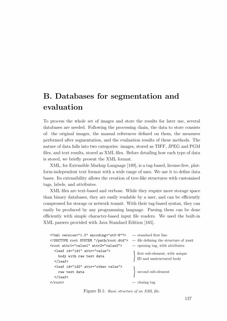
B. Databases for segmentation and
evaluation
To process the whole set of images and store the results for later use, several
databases are needed. Following the processing chain, the data to store consists
of: the original images, the manual references defined on them, the measures
performed after segmentation, and the evaluation results of these methods. The
nature of data falls into two categories: images, stored as TIFF, JPEG and PGM
files, and text results, stored as XML files. Before detailing how each type of data
is stored, we briefly present the XML format.
XML, for Extensible Markup Language [189], is a tag-based, license-free, plat-
form-independent text format with a wide range of uses. We use it to define data
bases. Its extensibility allows the creation of tree-like structures with customised
tags, labels, and attributes.
XML files are text-based and verbose. While they require more storage space
than binary databases, they are easily readable by a user, and can be efficiently
compressed for storage or network transit. With their tag-based syntax, they can
easily be produced by any programming language. Parsing them can be done
efficiently with simple character-based input file readers. We used the built-in
XML parsers provided with Java Standard Edition [165].
<?xml version="1.0" encoding="utf-8"?> ← standard first line
<!DOCTYPE root SYSTEM "/path/root.dtd"> ← file defining the structure of root
<root attr1="value1" attr2="value2"> ← opening tag, with attributes
<leaf id="id1" attr="value">
body with raw text data
</leaf>
first sub-element, with unique
ID and unstructured body
<leaf id="id2" attr="other value">
raw text data
</leaf>
second sub-element
</root> ← closing tag
Figure B.1: Basic structure of an XML file.
137

Appendix B. Databases for segmentation and evaluation
Original images
DAPI TIFF
FITC TIFF
Conversion
Input groups
DAPI JPEG, XML
FITC JPEG, XML
User input//
Segmentation
Comets references
XML references
Segmentation results
DAPI JPEG
FITC JPEG
XML output
Evaluation //
Analysis
Evaluation of
segmentation results
XML evaluation
Statistics
on individuals
XML stats
Figure B.2: Databases and process flows: the databases used during the processing are shown
as boxes, and the processes between them as arrows.
Figure B.2 shows a summary of the databases used in our system, and the
processes between them.
B.1 Original images and input groups
The original images are grayscale TIFF files, with intensity values encoded with
12 bits per pixel. They are arranged in pairs DAPI-FITC, and form the first
image database, organised by individuals and sets (see Section III.3 for details).
For display, the original images converted into 8 bit JPEG files. These files
are only used for visual inspection by users, and the loss of data due to the image
dimming is visually small. For processing though, they are also converted into 12
bit PGM files. It is a non-proprietary format, which can easily be read by most
138

Appendix B. Databases for segmentation and evaluation
programming languages. Only these files, forming the second image database,
will be used by our programs, for display and processing. Should a system failure
occur and files get corrupted, the original images would not be affected, and
would be used to rebuild the second database. We call one input group the set of
four images (DAPI JPEG, DAPI PGM, FITC JPEG, FITC PGM) corresponding
to one view.
B.2 Comets references
<?xml version="1.0" encoding="utf-8"?>
<!DOCTYPE reference SYSTEM "/telomeres/references.dtd">
<reference image="/MT002/MT002-1/1AG0000001" nbOfReferences="2">
<comets id="c1" nbOfPoints="302">
227 738 3.803030303030303 26.816120133932465
227 739 3.787878787878788 26.865458004681624
(...)
</comets>
<comets id="c2" nbOfPoints="335">
774 512 3.1622776601683795 22.608380316123238
774 513 3.1622776601683795 22.655732286889524
(...)
</comets>
</reference>
Figure B.3: Reference database: XML file storing the references for an input group.
The references for segmentation are defined as Comets. As explained in Sec-
tion IV.2, one Comets is defined by its border points, and the inner and outer
confidence factors at each border point. This is enough to build a confidence map
of any size, either for display or processing. The references for each input group
are stored in a distinct XML file. Figure B.3 shows an extract of such a file. The
root reference has two attributes: the name of the corresponding input group,
and the number of references defined. Each reference is stored as a sub-element
nucleus; its attributes are a unique identifier and the number of vertices defined
by the user. The body inside a nucleus lists the vertices’ x and y coordinates,
their inner and their outer confidence factors.
B.3 Segmentation results
A complete processing of one input group results in:
- a segmentation of the nuclei in the DAPI image,
139
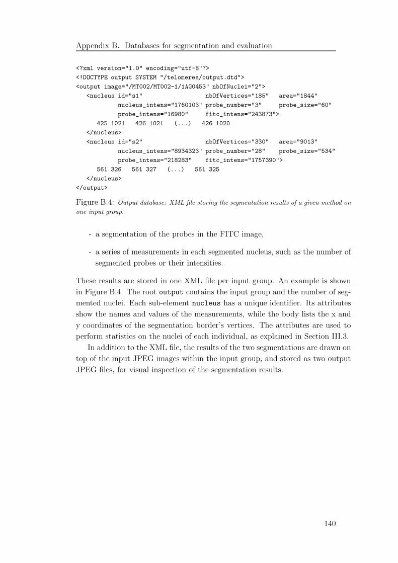
Appendix B. Databases for segmentation and evaluation
<?xml version="1.0" encoding="utf-8"?>
<!DOCTYPE output SYSTEM "/telomeres/output.dtd">
<output image="/MT002/MT002-1/1AG0453" nbOfNuclei="2">
<nucleus id="s1" nbOfVertices="185" area="1844"
nucleus_intens="1760103" probe_number="3" probe_size="60"
probe_intens="16980" fitc_intens="243873">
425 1021 426 1021 (...) 426 1020
</nucleus>
<nucleus id="s2" nbOfVertices="330" area="9013"
nucleus_intens="8934323" probe_number="28" probe_size="534"
probe_intens="218283" fitc_intens="1757390">
561 326 561 327 (...) 561 325
</nucleus>
</output>
Figure B.4: Output database: XML file storing the segmentation results of a given method on
one input group.
- a segmentation of the probes in the FITC image,
- a series of measurements in each segmented nucleus, such as the number of
segmented probes or their intensities.
These results are stored in one XML file per input group. An example is shown
in Figure B.4. The root output contains the input group and the number of seg-
mented nuclei. Each sub-element nucleus has a unique identifier. Its attributes
show the names and values of the measurements, while the body lists the x and
y coordinates of the segmentation border’s vertices. The attributes are used to
perform statistics on the nuclei of each individual, as explained in Section III.3.
In addition to the XML file, the results of the two segmentations are drawn on
top of the input JPEG images within the input group, and stored as two output
JPEG files, for visual inspection of the segmentation results.
140

Appendix B. Databases for segmentation and evaluation
B.4 Evaluation of segmentation results
<?xml version="1.0" encoding="utf-8"?>
<!DOCTYPE evaluation SYSTEM "/telomeres/evaluation.dtd">
<evaluation image="/MT002/MT002-1/1AG0000001" nbOfEntries="2">
<entry ref="c1" segm="s1">
<measure name="Comets" value="0.206901472150592"/>
<measure name="DSC" value="0.9280057968014078"/>
<measure name="Hausdorff" value="11.180339887498949"/>
<measure name="MeanHausdorff" value="3.93771243290371"/>
<measure name="StdDevHausdorff" value="4.130745785111794"/>
<measure name="RAO" value="0.865681730397837"/>
<measure name="RUMA" value="1.0"/>
</entry>
<entry ref="c2" segm="s2">
<measure name="Comets" value="0.19796783664006048"/>
<measure name="DSC" value="0.9269553975436329"/>
<measure name="Hausdorff" value="14.142135623730951"/>
<measure name="MeanHausdorff" value="4.171888719835954"/>
<measure name="StdDevHausdorff" value="4.574401197104007"/>
<measure name="RAO" value="0.863855421686747"/>
<measure name="RUMA" value="1.0"/>
</pair>
</evaluation>
Figure B.5: Evaluation database: XML file storing the evaluation of the segmentation results
for one input group.
The final database we use contains the results of the evaluation of a segmenta-
tion method. As detailed in Section III.3, we use an error matrix to store the dis-
crepancies between references and segmented objects. Since this matrix is sparse,
we only store the entries corresponding to overlapping references and objects (i.e.
with a non-infinite Comets error). These entries are encoded in XML, with one
file per input group, as illustrated in Figure B.5. The root evaluation contains
the input group identifier and the number of matrix entries. Each sub-element
entry lists the corresponding reference and object identifiers (corresponding to
the entry’s coordinates in the error matrix), and its body lists the discrepancy
measures. Since more than one measure can be performed, we use a structured
body with sub-elements measure. Each of them has two attributes: the measure’s
name and value.
141
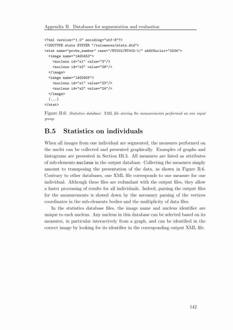
Appendix B. Databases for segmentation and evaluation
<?xml version="1.0" encoding="utf-8"?>
<!DOCTYPE stats SYSTEM "/telomeres/stats.dtd">
<stat name="probe_number" case="/MT002/MT002-1/" nbOfNuclei="3234">
<image name="1AG0453">
<nucleus id="s1" value="3"/>
<nucleus id="s2" value="28"/>
</image>
<image name="1AG0455">
<nucleus id="s1" value="23"/>
<nucleus id="s2" value="24"/>
</image>
(...)
</stat>
Figure B.6: Statistics database: XML file storing the measurements performed on one input
group.
B.5 Statistics on individuals
When all images from one individual are segmented, the measures performed on
the nuclei can be collected and presented graphically. Examples of graphs and
histograms are presented in Section III.3. All measures are listed as attributes
of sub-elements nucleus in the output database. Collecting the measures simply
amount to transposing the presentation of the data, as shown in Figure B.6.
Contrary to other databases, one XML file corresponds to one measure for one
individual. Although these files are redundant with the output files, they allow
a faster processing of results for all individuals. Indeed, parsing the output files
for the measurements is slowed down by the necessary parsing of the vertices
coordinates in the sub-elements bodies and the multiplicity of data files.
In the statistics database files, the image name and nucleus identifier are
unique to each nucleus. Any nucleus in this database can be selected based on its
measures, in particular interactively from a graph, and can be identified in the
correct image by looking for its identifier in the corresponding output XML file.
142

C. Porting image processing to a cluster
C.1 Architecture
We implemented all our programs on a Mac OS X cluster with 16 dual-G5 nodes.
Porting an image-processing program to a cluster can be achieved in different
ways. Common methods are listed below:
1. Divide an image into several parts, have each part processed on a distinct
node, and combine the results to obtain the processed image.
2. Divide the processing of one image into parallel steps, execute each step on
a distinct node, and combine the results to obtain the processed image.
3. Divide the processing of one image into successive steps, execute each step
on a given node, and have one node send its results to another node for the
following step. This corresponds to a pipe of nodes specialised in one step,
where the processed images are the output of the last node.
4. Divide the database into smaller groups of images, have each node process
one group.
The first strategy cannot be applied to our segmentation methods. As described
before, the segmentation of one image is based its entire contents. Splitting
an image would also unavoidably clip nuclei into distinct subimages, and thus
require extra processing to recover them afterwards. The second strategy is not
adapted to our processing either. We use successive processing steps, which
cannot run in parallel. The third strategy is only efficient when all the processing
steps take approximately the same time to execute. This is not the case of our
processing. In particular the segmentation nuclei is significantly longer than the
probe segmentation. Using pipes of nodes would result in delays and sub-optimal
use of the computing power.
The final strategy is better suited to our needs. The database of images we
143

Appendix C. Porting image processing to a cluster
Servers
Client 1
Client 2
· · ·
Client 16
Head Node
Node 2
· · ·
Node 16
Figure C.1: Client-Server architecture: location of the main processes on the cluster nodes.
use contains nearly 3,000 images, which is far greater than the number of nodes
in our cluster. However, dividing the database into 16 groups beforehand has two
main drawbacks. First, some nodes may finish their batch earlier than others,
but they would not be able to help them process their remaining images, thus
wasting processing time. Second and more importantly, should a system failure
occur on a node, all the images which were to be processed there would remain
unprocessed at the end. Thus, it would be non-efficient and not robust. To avoid
these two issues, we implemented a strategy based on a dynamic task allocation,
with a client-server architecture.
The server is used only to distribute the images for processing. Each client
requests an image from the server, processes it on its own, then send the processed
image back, and requests another image. For programming reasons, each client
communicates with a dedicated server, which in turns communicate with the
main server. The servers are light processes and can run on the same cluster
node as another client (See Figure C.1). Slight bottlenecks could happen in case
many clients require an image at the same time. In practice however, since each
node takes a different time to process its current image, the image requests occur
at different times, and clients never have to wait significantly to obtain another
image to process.
This way, all clients are busy at all time, until the server reaches the end of
the database. This strategy ensures an optimal use of computation time on all
the nodes of the cluster. Besides, in case of system failure on a node, the server
will keep sending the remaining images to all other nodes. Only the image being
processed at the time of the failure will be unprocessed. At the end the server
will easily identify unprocessed images, and reassign them to an active node. Our
strategy ensures an optimal and robust use of the cluster computing power.
144

Appendix C. Porting image processing to a cluster
C.2 Protocols
The protocols we use rely on exchanges of bytes between the communicating
processes: either single bytes for standard messages, strings for file names, or
arrays of bytes for file contents. Opening sockets and exchanging bytes over
them can be programmed with the standard Java classes for input and output.
We use five protocols: one to start the communications, one to transfer a
file, one to convert files from TIFF to PGM and JPEG, one to segment an input
group, and one to end communications. They are presented in Tables C.1 to C.2.
In these tables, the vertical dots indicate that a process is waiting to receive
a network message, and the arrows show which process is sending a message
to which. The standard messages we use are encoded as different bytes. For
readability, we use names, in small capitals, instead of values to present them
in the tables below. They are: request task, sending file, file received,
convert, segment, end.
Table C.1: Protocol for communication opening.
Main Server Dedicated Server i Client i
start start... oo ask for connection
launch // start...
... register connection // connect
...... oo send request task
... oo send request task...
prepare a task...
...
Table C.2: Protocol for communication ending.
Main Server Dedicated Server i Client i
send end //...
...... send end //
...... close connections close connections... end thread end thread
145

Appendix C. Porting image processing to a cluster
Table C.3: Protocol for file transfer.
Sender Receiver...
send sending file // prepare for reception
send file name // store file name
send file size // store file size
send file contents // store file contents
prepare to compare oo send file received
... oo send local file size
compare with original file size...
- if different, start over
- else, proceed to next step
Summarised as:
send file // store file
Table C.4: Protocol for the conversion task.
Main Server Dedicated Server i Client i
send convert //...
...
send convert // prepare for conversion
send file names // find the files...
... send tiff files // store files
...... convert files
... store files oo send jpeg, pgm files
...... oo send request task
... oo send request task...
prepare a task...
...
146

Appendix C. Porting image processing to a cluster
Table C.5: Protocol for the segmentation task.
Main Server Dedicated Server i Client i
send segment //...
...
send segment // prepare for segmentation
send input
group name// find the files
...
... send jpeg, xml files // store files
...... segment images
... store files oo send jpeg, xml files
...... oo send request task
... oo send request task...
prepare a task...
...
C.3 Results and discussion
The architecture and protocols presented above allow any number of clients to
connect to the main server, at any time, and minimise the losses in case of a
client failure. In particular, clients can be started on any computer connected
to the cluster, and more than one client can be started on any computer. In
this section we discuss the effect of running multiple clients on the cluster nodes.
We performed the conversion and segmentation of the whole data base with 1,
2, and 3 clients running per node. We present the average elapsed time spent
by each client on each image, detailed for each subtask of the conversion and
the segmentation, in Figure C.2. The head node is equipped with 1Gb RAM,
while the other nodes have 256 Mb RAM each. As they have a slightly different
configuration, we present the results averaged over all clients, then over all clients
on the head node, and over all clients on the other nodes. The total elapsed times
needed to process the whole database are presented in Table C.6.
Table C.6: Total elapsed time to process the whole database on the cluster, depending on the
number of clients running per node.
1 client 2 clients 3 clients 2 clients with compression
Conversion 23’ 49” 22’ 08” 29’ 39” 21’ 06”
Segmentation 35’ 30” 36’ 57” 60’ 33” 66’ 10”
Judging from Figure C.2, adding clients on a node slows the processing down.
The effect is less severe on the head node, where more memory is available, than
147

Appendix C. Porting image processing to a cluster
Figure C.2: Processing times as functions of the number of clients running per node, perform-
ing conversion (left column) and segmentation (right column). The top row shows the average
time per client, the middle row per client on the head node, and the bottom row per client on
the other nodes.
148

Appendix C. Porting image processing to a cluster
on the other nodes. In addition to competing for memory and CPU time, the
clients also compete for network bandwidth. Adding more clients degrades the
time needed to upload a converted input group: the operation is about 12 times
slower on average with three clients than with one. Similarly, it affects the time
needed to download an input group prior to segmentation: it is about 30 times
slower with three clients than with one.
Adding more clients increases the time spent to process an image, but also
reduces the total number of images processed by each client, as they share the
load. Overall, the total time needed to process the whole database, either for
conversion or segmentation, in Table C.6, is similar with one and two clients per
node, but significantly higher with three clients per node. In the latter case,
most of the time is spent on uploading and downloading data over the network.
Copying the whole database on each node prior to processing would be against
the flexibility provided by the architecture, as it would prevent the later addition
of extra nodes to the cluster, and would require a significant amount of time and
space, while duplicating a database in sixteen copies and causing maintenance
issues. Another solution consists in compressing the files prior to transmitting
them over the network. Compression is easily implementable with the standard
Java distribution. We experimented file compression running two clients per
node. Although the total conversion time is smaller (21’ 06”), segmentation is
significantly higher (66’ 10”). This is due to the decompression step needed prior
to segmentation. In our context, conversion is performed once on the whole
database, while segmentation is performed as many times as needed for tuning
and comparison of different methods. The small gain of conversion time is thus
not enough to balance the large loss of segmentation time. We decided to perform
all the tasks with one single client per node, and without any compression.
149
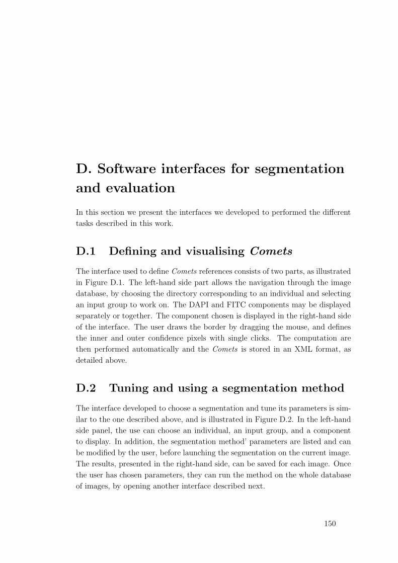
D. Software interfaces for segmentation
and evaluation
In this section we present the interfaces we developed to performed the different
tasks described in this work.
D.1 Defining and visualising Comets
The interface used to define Comets references consists of two parts, as illustrated
in Figure D.1. The left-hand side part allows the navigation through the image
database, by choosing the directory corresponding to an individual and selecting
an input group to work on. The DAPI and FITC components may be displayed
separately or together. The component chosen is displayed in the right-hand side
of the interface. The user draws the border by dragging the mouse, and defines
the inner and outer confidence pixels with single clicks. The computation are
then performed automatically and the Comets is stored in an XML format, as
detailed above.
D.2 Tuning and using a segmentation method
The interface developed to choose a segmentation and tune its parameters is sim-
ilar to the one described above, and is illustrated in Figure D.2. In the left-hand
side panel, the use can choose an individual, an input group, and a component
to display. In addition, the segmentation method’ parameters are listed and can
be modified by the user, before launching the segmentation on the current image.
The results, presented in the right-hand side, can be saved for each image. Once
the user has chosen parameters, they can run the method on the whole database
of images, by opening another interface described next.
150
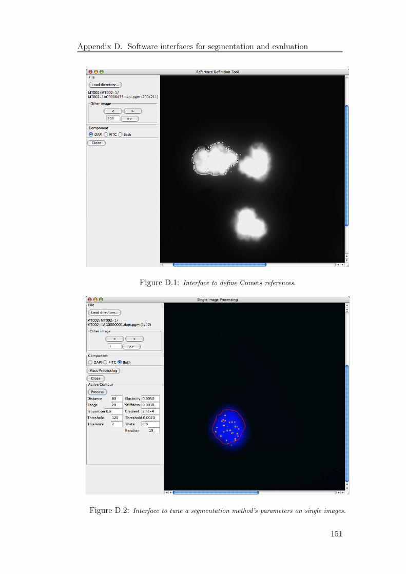
Appendix D. Software interfaces for segmentation and evaluation
Figure D.1: Interface to define Comets references.
Figure D.2: Interface to tune a segmentation method’s parameters on single images.
151

Appendix D. Software interfaces for segmentation and evaluation
D.3 Visualising the processing on a cluster
As described above in this chapter, the clients open connections with the main
server and receive orders from it, through dedicated servers. A light addition
to the protocols described above allows the clients to pass messages to the main
server at any time. These messages can be visualised in real-time.
The interface used to visualise the current status of all nodes on the cluster
is presented in Figure D.3. On the left-hand side panel, the proportion of images
processed overall and per individual is presented graphically, along with the total
elapsed time. The right-hand side panel shows information on the clients: their
current status, as reported from them, and the number of images they have
processed.
Figure D.3: Interface to visualise the status of all nodes processing images on a cluster.
152

Appendix D. Software interfaces for segmentation and evaluation
D.4 Visualising measures on different individu-
als
The final interface we present here is used to display the various measures per-
formed on the individuals in our data base, as detailed in Chapter III. It is
illustrated in Figure D.4. In the left-hand side panel, the user can choose one or
more individual, the values to display, and the bin size of the histograms. Other
options allow filtering nuclei that are clipped at the edges of an image, and listing
the number of nuclei segmented for each individual.
Figure D.4: Interface to visualise the measures on different individuals.
153
Bibliography
[1] Wael Abd-Almageed, Christopher E. Smith, and Samah Ramadan. Kernel
snakes: Non-parametric active contour models. In International Conference
on Systems, Man, and Cybernetics, volume 1, pages 240–244, Washington,
DC, USA, October 2003.
[2] David Adalsteinsson and James A. Sethian. A fast level set method for
propagating interfaces. Journal of Computational Physics, 118(2):269–277,
May 1995.
[3] Dwi Anoraganingrum. Cell segmentation with median filter and mathemat-
ical morphology operation. In International Conference on Image Analysis
and Processing, pages 1043–1046, Venice, Italy, September 1999.
[4] A. Antsaklis, N. Papantoniou, S. Mesogitis, S. Michalas, and D. Aravanti-
nos. Pregnant women of 35 years of age or more: maternal serum markers
or amniocentesis? Journal of Obstetrics and Gynaecology, 19(3):253–256,
May 1999.
[5] Tatiana Babochkina, Susanne Mergenthaler, Guiseppina De Napoli, Sashka
Hristoskova, Sevgi Tecanli, Wolfgang Holzgreve, and Sinuhe Hahn. Numer-
ous erythroblasts in maternal blood are impervious to fluorescent in situ
hybridization analysis, a feature related to a dense compact nucleus with
apoptic character. Haematologica, 90(6):739–744, 2005.
[6] Gabriela M. Baerlocher, Jennifer Mak, Teri Tien, and Peter M. Lansdorp.
Telomere length measurements by fluorescence in situ hybridization and
flow cytometry: tips and pitfalls. Cytometry, 47:89–99, 2002.
[7] EunSang Bak, Kayvan Najarian, and John P. Brockway. Efficient segmen-
tation framework of cell images in noise environments. Technical report,
Memory Testing Corporation, USA, 2004.
[8] Lucia Ballerini and Leonardo Bocchi. Segmentation of liver images by
texture and genetic snakes. In European Medical and Biological Engineering
Conference, Vienna, Austria, December 2002.
[9] Lucia Ballerini and Leonardo Bocchi. Bone segmentation using multiple
communicating snakes. In SPIE Medical Imaging, volume 5032, pages 1621–
1628, San Diego, CA, USA, February 2003.
[10] Pascal Bamford. Segmentation of Cell Images With Application to Cervical
Cancer Screening. PhD thesis, University of Queensland, 1999.
154

Bibliography
[11] Pascal Bamford. Automating cell segmentation evaluation with annotated
examples. In APRS Workshop on Digital Image Computing, pages 21–25,
Brisbane, Australia, February 2003.
[12] Pascal Bamford and Brian Lovell. Method for accurate unsupervised cell
nucleus segmentation. In IEEE Engineering in Medicine and Biology, vol-
ume 1, pages 133–137, Istanbul, Turkey, October 2001.
[13] Julian Besag. On the statistical analysis of dirty pictures. Journal of the
Royal Statistical Society. Series B, 48(3):259–302, 1986.
[14] S. Beucher. The watershed transformation applied to image segmentation.
Scanning Microscopy, 6:299–314, 1992.
[15] Andrew Blake and Michael Isard. Active Contours. Springler-Verlag, 1998.
ISBN 3-540-76217-5.
[16] W. Bocker, H-W Gantenberg, W-U Muller, and C. Streffer. Automated cell
cycle analysis with fluorescence microscopy and image analysis. Physics in
Medicine and Biology, 41:523–537, 1996.
[17] Yuri Y. Boykov and Marie-Pierr Jolly. Interactive graph cuts for optimal
boundary and region segmentation of objects in n-d images. In Interna-
tional Conference on Computer Vision, volume 1, pages 105–112, Vancou-
ver, Canada, July 2001.
[18] Jorg Bredno, Thomas M. Lehmann, and Klauss Spitzer. A general finite
element model for segmentation in 2, 3, and 4 dimensions. In SPIE Medical
Imaging, volume 3979, pages 1174–1184, San Diego, CA, USA, February
2000.
[19] Jorg Bredno, Thomas M. Lehmann, and Klauss Spitzer. A general discrete
contour model in two, three and four dimensions for topology-adaptive
multichannel segmentation. IEEE Transactions on Pattern Analysis and
Machine Intelligence, 25(5):550–563, May 2003.
[20] Patrick Brigger, Jeff Hoeg, and Michael Unser. B-spline snakes: A flex-
ible tool for parametric contour detection. IEEE Transactions on Image
Processing, 9(9):1484–1496, September 2000.
[21] Patrick Brigger, Frank Muller, Klaus Illgner, and Michael Unser. Cen-
tered pyramids. IEEE Transactions on Image Processing, 8(9):1254–1264,
September 1999.
155

Bibliography
[22] Tim H. Brummendorf, Jaroslaw P. Maciejewski, Jennifer Mak, Neal S.
Young, and Peter M. Lansdorp. Telomere length in leukocyte subpopu-
lations of patients with aplastic anemia. Blood, 97(4):895–900, 2001.
[23] Peter J. Burt and Edward H. Adelson. The Laplacian pyramid as a compact
image code. IEEE Transactions on Communications, COM-31(4):532–540,
April 1983.
[24] Kerstin Bystricky, Patrick Heun, Lutz Gehlen, Jorg Langowski, and Su-
san M. Gasser. Long-range compaction and flexibility of interphase chro-
matin in budding yeast analyzed by high-resolution imaging techniques.
PNAS, 101(47):16495–16500, November 2004.
[25] Nigel P. Carter. Fluorescence in situ hybridization – state of the art.
Bioimaging, 4:41–51, 1996.
[26] Vicent Caselles, Ron Kimmel, and Guillermo Sapiro. Geodesic active con-
tours. In International Conference on Computer Vision, pages 694–699,
Boston, MA, USA, June 1995.
[27] Vincent Caselles, Ron Kimmel, and Guillermo Sapiro. Geodesic active
contours. International Journal of Computer Vision, 22(1):61–79, February
/ March 1997.
[28] D. Casey, C. Cantor, and S. Spengler. Primer on molecular genetics. Tech-
nical report, US Department of Energy, DOE Human Genome Project, Oak
Ridge National Laboratory, 1060 Commerce Park, Oak Ridge, TN 37830,
June 1992.
[29] Francis H.Y. Chan, F.K. Lam, and Hui Zhu. Adaptive thresholding by
variational method. IEEE Transactions on Image Processing, 7(3):468–473,
March 1998.
[30] Su Chen and Robert Haralick. Recursive erosion, dilation, opening, and
closing transforms. IEEE Transactions on Image Processing, 4(3):335–345,
March 1995.
[31] Xiaohua Chen, Michael Brady, and Daniel Rueckert. Simultaneous segmen-
tation and registration for medical image. In Medical Image Computing
and Computer-Assisted Intervention, volume 1, pages 663–670, Saint-Malo,
France, September 2004.
156
Bibliography
[32] Yunmei Chen, Feng Huang, Hemant D. Tagare, Murali Rao, David Wilson,
and Edward A. Geiser. Using prior shape and intensity profile in medi-
cal image segmentation. In International Conference on Computer Vision,
pages 1117–1124, Nice, France, October 2003.
[33] Yunqiang Chen, Thomas S. Huang, and Yong Rui. Optimal radial contour
tracking by dynamic programming. In International Conference on Image
Processing, volume 1, pages 626–629, Thessaloniki, Greece, October 2001.
[34] Ward Cheney and David Kincaid. Numerical Mathematics and Computing.
Brooks/Cole Publishing, fourth edition, 1999. ISBN 0-534-35184-0.
[35] William F. Clocksin. Automatic segmentation of overlapping nuclei with
high background variation using robust estimation and flexible contour
models. In International Conference on Image Analysis and Processing,
pages 682–687, Mantova, Italy, September 2003.
[36] William F. Clocksin and Boaz Lerner. Automatic analysis of fluorescence
in-situ hybridisation images. In British Machine Vision Conference, pages
666–674, Bristol, UK, September 2000.
[37] Laurent D. Cohen. On active contour models and balloons. Computer
Vision, Graphics, and Image Processing: Image Understanding, 53(2):211–
218, March 1991.
[38] Timothy F. Cootes, Gareth J. Edwards, and Christopher J. Taylor. Com-
paring active shape models with active appearance models. In British Ma-
chine Vision Conference, pages 173–182, Nottingham, UK, September 1999.
[39] Timothy F. Cootes and Christopher J. Taylor. Statistical models of ap-
pearance for medical image analysis and computer vision. In SPIE Medical
Imaging, volume 4322, pages 236–248, San Diego, CA, USA, February 2001.
[40] Timothy F. Cootes, Carole J. Twining, Vladimir Petrovic, Roy Schestowitz,
and Christopher J. Taylor. Groupwise construction of appearance models
using piece-wise affine deformations. In British Machine Vision Conference,
volume 2, pages 879–888, Oxford, UK, September 2005.
[41] Timothy F. Cootes, Carole J. Twining, and Christopher J. Taylor. Diffeo-
morphic statistical shape models. In British Machine Vision Conference,
volume 1, pages 447–456, London, UK, September 2004.
[42] Thomas H. Cormen, Charles E. Leiserson, and Ronald L. Rivest. Introduc-
tion to Algorithms. Addison Wesley, first edition, 1990. ISBN 0-262-03141-8.
157

Bibliography
[43] William R. Crum, Oscar Camara, Daniel Rueckert, Mark Jenkinson, and
Derek L.G. Hill. Evaluating atlas segmentation of multiple structures using
generalised measures of region overlap. In Medical Image Understanding
and Analysis, pages 163–166, Bristol, UK, July 2005.
[44] Michael B. Dillencourt, Hannan Samet, and Markku Tamminen. A general
approach to connected-component labeling for arbitrary image representa-
tions. Journal of the Association for Computing Machinery, 39(2):253–280,
April 1992.
[45] Edward Dougherty and Roberto Lotufo. Hands-on Morphological Image
Processing, volume TT59, chapter 5 Gray-Scale Morphology, pages 81–120.
SPIE, July 2003.
[46] Edward Dougherty and Roberto Lotufo. Hands-on Morphological Image
Processing, volume TT59, chapter 6 Morphological Process of Gray-Scale
Images, pages 121–138. SPIE, July 2003.
[47] Edward Dougherty and Roberto Lotufo. Hands-on Morphological Image
Processing, volume TT59, chapter 7 Morphological Segmentation - Water-
shed, pages 139–154. SPIE, July 2003.
[48] Nick Efford. Digital Image Processing – a practical introduction using Java.
Addison Wesley, 2000. ISBN: 0-201-59623-7.
[49] M. Egmont-Petersen, D. de Ridder, and H. Handels. Image processing with
neural networks – a review. Pattern Recognition, 35:2279–2301, 2002.
[50] Bing Fang, Wynne Hsu, and Mong Li Lee. On the accurate counting of
tumor cells. IEEE Transactions on Nanobioscience, 2(2):94–103, June 2003.
[51] Pedro F. Felzenszwalb and Daniel P. Huttenlocher. Distance transforms of
sampled functions. Technical report, Cornell University, September 2004.
TR2004-1963.
[52] Samuel D. Fenster, Chun-Bin Gary Kuo, and John R. Kender. Nonpara-
metric training of snakes to find indistinct boundaries. In CVPR Workshop
on Mathematical Methods in Biomedical Image Analysis, Kauai, Hawaii,
USA, December 2001.
[53] Alban Foulonneau, Pierre Charbonnier, and Fabrice Heitz. Affine-invariant
multi-reference shape priors for active contours. In Ales Leonardis, Horst
Bischof, and Axel Pinz, editors, European Conference on Computer Vision,
volume 3952 of LNCS, pages 601–613. Springer, 2006.
158

Bibliography
[54] Guido Gerig, Matthieu Jomier, and Miranda Chakos. Valmet: A new val-
idation tool for assessing and improving 3D object segmentation. In Med-
ical Image Computing and Computer-Assisted Intervention, Utrecht, The
Netherlands, October 2001.
[55] V. Grau, A.U.J. Mewes, M. Alcaniz, R. Kikinis, and S.K. Warfield. Im-
proved watershed transform for medical image segmentation using prior
information. IEEE Transactions on Medical Imaging, 23(4):447–458, 2004.
[56] W.E.L. Grimson, Michael E. Leventon, Olivier Faugeras, and William
Wells. Computer vision methods for image guided surgery. In British Ma-
chine Vision Conference, pages 1–12, Bristol, UK, September 2000.
[57] Yu Guo, Sebrina Levesque, Thomas Manfred, and Ying Sun. Automated
detection and delineation of mitochondria in electron micrographs of hu-
man skeletal muscles. Microscopy research and technique, 63(3):133–139,
February 2004.
[58] James E. Haddow, Glenn E. Palomaki, George J. Knight, George C. Cun-
ningham, Linda S. Lustig, and Patricia A. Boyd. Reducing the need for
amniocentesis in women 35 years of age or older with serum markers for
screening. New England Journal of Medicine, 330:1114–1118, April 1994.
[59] Sinuhe Hahn and Wolfgang Holzgreve. Fetal cells and Fetal DNA in ma-
ternal blood. Karger, Basel, Switzerland, 2001.
[60] Sinuhe Hahn, Rosalie Sant, and Wolfgang Holzgreve. Fetal cells in maternal
blood: current and future perspectives. Molecular Human Reproduction,
4(6):515–521, 1998.
[61] Ghassan Hamarneh, Tim McInerney, and Dimitri Terzopoulos. Deformable
organisms for automatic medical image analysis. In Medical Image Comput-
ing and Computer-Assisted Intervention, pages 66–75, Utrecht, The Nether-
lands, October 2001.
[62] Xiao Han, Chenyang Xu, and Jerry L. Prince. A topology preserving level
set method for geometric deformable models. IEEE Transactions on Pat-
tern Analysis and Machine Intelligence, 25(6):755–768, June 2003.
[63] Calvin B. Harley, A. Bruce Futcher, and Carol W. Greider. Telomeres
shorten during ageing of human fibroblasts. Nature, 345(6274):458–460,
May 1990.
159

Bibliography
[64] Harald Hohmann, Susanne Michel, Wolfgang Reiber, Michael Gunther, Uwe
Claussen, and Ferdinand von Eggeling. How to enrich and analyse fetal cells
from maternal blood: 5-year experience with PCR, FISH and cultivation.
In Fetal Cells and Fetal DNA in Maternal Blood - New Developments for a
New Millennium, pages 47–55. Karger, 2001.
[65] Wolfgang Holzgreve, Xiao Yan Zhong, Carolyn Troeger, Isabelle Haari, Vi-
vian Kiefer, and Sinuhe Hahn. Fetal cells in maternal blood: An overview
of the Basel experience. In Fetal Cells and Fetal DNA in Maternal Blood -
New Developments for a New Millennium, pages 28–36. Karger, 2001.
[66] Adam Hooverand, Gillian Jean-Baptiste, Xiaoyi Jiang, Patrick J. Flynn,
Horst Bunke, Dmitry B. Goldgof, Kevin Bowyer, David W. Eggert, Andrew
Fitzgibbon, and Robert B. Fisher. An experimental comparison of range
image segmentation algorithms. IEEE Transactions on Pattern Analysis
and Machine Intelligence, 18(7):673–689, July 1996.
[67] Wu-Chih Hu and Hsin-Teng Sheu. Quadratic B-spline for curve fitting.
National Science Council Republic of China, 24(5):373–381, 2000.
[68] James P. Ivins. Statistical Snakes: Active Region Models. PhD thesis,
University of Sheffield, 1996.
[69] James P. Ivins and John Porrill. Everything you always wanted to know
about snakes (but were afraid to ask). Technical report, AIVRU, University
of Sheffield, March 2000.
[70] Mathews Jacob. Parametric Shape Processing in Biomedical Imaging. PhD
thesis, Ecole Polytechnique federale de Lausanne, 2003.
[71] Torsten Jarkrans. Algorithms for Cell Image Analysis in Cytology and
Pathology. PhD thesis, Uppsala University, 1996.
[72] Stephanie Jehan-Besson and Michel Barlaud. DREAM2S: deformable re-
gions driven by an Eulerian accurate minimization method for image and
video segmentation. International Journal of Computer Vision, 53(1):45–
70, 2003.
[73] Stephanie Jehan-Besson, Michel Barlaud, Gilles Aubert, and Olivier
Faugeras. Shape gradients for histogram segmentation using active con-
tours. In International Conference on Computer Vision, pages 408–415,
Nice, France, October 2003.
160

Bibliography
[74] Dong Joong Kang. A fast and stable snake algorithm for medical images.
Pattern Recognition Letters, 20:507–512, 1999.
[75] Martin Kerschner. Homologous twin snakes integrated in a bundle block
adjustment. In Symposium on Object Recognition and Scene Classifica-
tion from Multispectral and Multisensor Pixels, volume 32, pages 244–249,
Colombus, Ohio, USA, July 1998.
[76] Jeong-Gyoo Kim and J. Alison Noble. Modelling an average shape. In
Medical Image Understanding and Analysis, pages 65–68, Sheffield, UK,
July 2003.
[77] Pushmeet Kohli and Philip H.S. Torr. Measuring uncertainty in graph
cut solutions - efficiently computing min-marginal energies using dynamic
graph cuts. In European Conference on Computer Vision, pages 30–43,
Graz, Austria, May 2006.
[78] A. Kolialexi, G. T. Tsangaris, A. Antsaklis, S. Kitsiou-Tzeli, and
A. Mavrou. Use of annexin v for the identification of fetal cells in ma-
ternal circulation. In Vivo, 18(5):629–632, September-October 2004.
[79] Vladimir Kolmogorov and Ramin Zabih. What energy functions can be
minimized via graph cuts? IEEE Transactions on Pattern Analysis and
Machine Intelligence, 26(2):147–159, February 2004.
[80] Steen Kølvraa, Britta Christensen, Lene Lykke-Hansen, and John Philip.
The fetal erythroblast is not the optimal target for non-invasive prenatal di-
agnosis: preliminary results. Journal of Histochemistry and Cytochemistry,
53(3):331–336, March 2005.
[81] Domagoj Kovacevic, Sven Loncaric, and Erich Sorantin. Deformable con-
tour based method for medical image segmentation. In International Con-
ference on Information Technology Interfaces, pages 145–150, Zagreb, Croa-
tia, 1999.
[82] Gerald Kuhne, Joachim Weickert, Markus Beier, and Wolfgang Effelsberg.
Fast implicit active contour models. Pattern Recognition, 2449:133–140,
2002.
[83] B. Ravi Kumar, Danny K. Joseph, and T. T. Sreenivas. Teager energy
based blood cell segmentation. Digital Signal Processing, 2:619–622, July
2002.
161
Bibliography
[84] M. Pawan Kumar, Philip H.S. Torr, and Andrew Zisserman. Obj-cut. In
Computer Vision and Pattern Recognition, volume 1, pages 18–25, San
Diego, CA, USA, June 2005.
[85] Zoltan Kutalik, Moe Razaz, and Jozsef Baranyi. Automated spatial and
temporal image analysis of bacterial cell growth. In BMVA Symposium on
Spatiotemporal Image Processing, London, UK, March 2004.
[86] Peter M. Lansdorp, Nico P. Verwoerd, Frans M. van de Rijke, Visia
Dragowska, Marie-Terese Little, Roeland W. Dirks, Anton K. Raap, and
Hans J. Tanke. Heterogeneity in telomere length of human chromosomes.
Human Molecular Genetics, 5(5):685–691, 1996.
[87] Robert Lapp, Maria Lorenzo-Valdes, and Daniel Rueckert. 3D/4D car-
diac segmentation using active appearance models, non-rigid registration,
and the Insight tool. In Medical Image Computing and Computer-Assisted
Intervention, pages 419–426, Saint-Malo, France, September 2004.
[88] Ole Vilhelm Larsen, Petia Radeva, and Enric Marti. Guidelines for choosing
optimal parameters of elasticity for snakes. In International Conference
on Computer Analysis and Image Processing, volume 970, pages 106–113,
Prague, Czech Republic, September 1995.
[89] Sebastien Lefevre, Jean-Pierre Gerard, Aurelie Piron, and Nicole Vincent.
An extended snake model for real-time multiple object tracking. In Ad-
vanced Concepts for Intelligent Vision Systems, pages 268–275, Ghent, Bel-
gium, September 2002.
[90] Thomas Lehmann, Jorg Bredno, and Klauss Spitzer. On the design of
active contours for medical image segmentation. Methods of Information
in Medicine, 42(1):89–98, 2003.
[91] Thomas M. Lehmann. From plastic to gold: A unified classification scheme
for reference standards in medical image processing. In Medical Imaging
2002: Image Processing, volume 4684, pages 1819–1827, San Diego, CA,
USA, February 2002.
[92] Boaz Lerner, William F. Clocksin, Seema Dhanjal, Maj A. Hulten, and
Christopher M. Bishop. Automatic signal classification in fluorescence in
situ hybridization images. Cytometry, 43:87–93, 2001.
[93] Boaz Lerner, William F. Clocksin, Seema Dhanjal, Maj A. Hulten, and
Christopher M. Bishop. Feature representation and signal classification in
162

Bibliography
fluorescence in-situ hybridization image analysis. IEEE Transactions on
Systems, Man, and Cybernetics - Part A: Systems and Humans, 31(6):655–
665, November 2001.
[94] Michael E. Leventon, W.E.L. Grimson, and Olivier Faugeras. Statistical
shape influence in geodesic active contours. In Computer Vision and Pat-
tern Recognition, volume 1, pages 316–323, Hilton Head Island, South Car-
olina, USA, June 2000.
[95] Jeffrey M. Levsky and Robert H. Singer. Fluorescence in situ hybridization:
past, present and future. Journal of Cell Science, 116:2833–2838, 2003.
[96] Olivier Lezoray, Abder Elmoataz, Hubert Cardot, and Marinette Revenu.
A.R.C.T.I.C : Un systeme automatique de tri cellulaire par analyse
d’images. In Vision Interface, Trois-Rivieres, Canada, May 1999.
[97] Qingmin Liao and Yingying Deng. An accurate segmentation method for
white blood cell images. In International Symposium on Biomedical Imag-
ing, pages 245–248, Washington, DC, USA, July 2002.
[98] Gang Lin, Umesh Adiga, Kathy Olson, John Guzowski, Carol Barnes, and
Badrinath Roysam. A hybrid 3D watershed algorithm incorporating gradi-
ent cues and object models for automatic segmentation of nuclei in confocal
image stacks. Cytometry, 56A(1):23–36, November 2003.
[99] Marie-Terese Little, Sylvie Langlois, R. Douglas Wilson, and Peter M.
Lansdorp. Frequency of fetal cells in sorted subpopulations of nucleated
erythroid and cd34+ hematopoietic progenitor cells from maternal periph-
eral blood. Blood, 89(7):2347–2358, April 1997.
[100] Steven Lobregt and Max A. Viergever. A discrete dynamic contour model.
IEEE Transactions on Medical Imaging, 14(1):12–24, March 1995.
[101] Suhuai Luo, Rongxin Li, and Sebastien Ourselin. A new deformable model
using dynamic gradient vector flow and adaptive balloon forces. In APRS
Workshop on Digital Image Computing, pages 9–14, Brisbane, Australia,
February 2003.
[102] Mahnaz Maddah, Kelly H. Zou, William M. Wells, Ron Kikinis, and Si-
mon K. Warfield. Automatic optimization of segmentation algorithms
through simultaneous truth and performance level estimation (STAPLE).
In Medical Image Computing and Computer-Assisted Intervention, vol-
ume 1, pages 274–282, Saint-Malo, France, September 2004.
163
Bibliography
[103] Ravikanth Malladi, James A. Sethian, and Baba C. Vemuri. Shape mod-
eling with front propagation: A level set approach. IEEE Transactions on
Pattern Analysis and Machine Intelligence, 17(2):158–175, February 1995.
[104] Norberto Malpica, Carlos Ortiz de Solorzano, Juan Jose Vaquero, Andres
Santos, Isabel Vallcorba, Jose Miguel Garcıa-Sagrado, and Francisco del
Pozo. Applying watershed algorithms to the segmentation of clustered nu-
clei. Cytometry, 28:289–297, 1997.
[105] Matei Mancas and Bernard Gosselin. Fuzzy tumor segmentation based
on iterative watersheds. In ProRISC Workshop on Circuits, Systems and
Signal Processing, Veldhoven, the Netherlands, November 2003.
[106] Matei Mancas and Bernard Gosselin. Iterative watersheds and fuzzy tu-
mor visualization. In IEEE Visualization Conference, Seattle, Washington,
October 2003.
[107] Matei Mancas and Bernard Gosselin. Towards an automatic tumor segmen-
tation using iterative watersheds. In SPIE Medical Imaging, San Diego, CA,
USA, February 2004.
[108] Tim McInerney and Demetri Terzopoulos. Topologically adaptable snakes.
In International Conference on Computer Vision, pages 840–845, Boston,
MA, USA, June 1995.
[109] Tim McInerney and Demetri Terzopoulos. Deformable models in medical
image analysis: A survey. Medical Image Analysis, 1(2):91–108, 1996.
[110] Tim McInerney and Demetri Terzopoulos. Medical image segmentation
using topologically adaptable surfaces. In Computer Vision, Virtual Real-
ity and Robotics in Medicine and Medial Robotics and Computer-Assisted
Surgery, pages 23–32, Grenoble, France, March 1997.
[111] Tim McInerney and Demetri Terzopoulos. Topology adaptive deformable
surfaces for medical image volume segmentation. IEEE Transactions on
Medical Imaging, 18(10):840–850, October 1999.
[112] Alan K. Meeker, Wesley R. Gage, Jessica L. Hicks, Inpakala Simon,
Jonathan R. Coffman, Elizabeth A. Platz, Gerrun E. March, and Angelo M.
De Marzo. Telomere length assessment in human archival tissues. American
Journal of Pathology, 160(4):1259–1268, April 2002.
[113] Fatima A. Merchant and Kenneth R. Castleman. Strategies for automated
fetal cell screening. Human Reproduction Update, 8(6):509–521, 2002.
164

Bibliography
[114] Volker Metzler, Jorg Bredno, Thomas Lehmann, and Klauss Spitzer. A
deformable membrane for the segmentation of cytological samples. In SPIE
Medical Imaging, volume 3338, pages 1246–1257, San Diego, CA, USA,
February 1998.
[115] Volker Metzler, Thomas Lehmann, Hans Bienert, Khosrow Mottaghy, and
Klaus Spitzer. Scale-independent shape analysis for quantitative cytol-
ogy using mathematical morphology. Computers in Biology and Medicine,
30:135–151, 2000.
[116] James V. Miller, David E. Breen, William E. Lorensen, Robert M. O’Bara,
and Michael J. Wozny. Geometrically deformed models: A method for
extracting closed geometric models from volume data. Computer Graphics,
25(4):217–226, July 1991.
[117] Morton Nadler and Eric P. Smith. Pattern Recognition Engineering. Wiley-
Interscience, 1993. ISBN 0-471-62293-1.
[118] Y. Nakajima and S. Mori. Global and strict curve fitting method. In
International Workshop on Frontiers in Handwriting Recognition, pages
523–528, Amsterdam, The Netherlands, September 2000.
[119] Jacinto Nascimento and Jorge Marques. An adaptive potential for robust
shape estimation. In British Machine Vision Conference, pages 343–352,
Manchester, UK, September 2001.
[120] A. Nedzved, S. Ablameyko, and I. Pitas. Morphological segmentation of
histology cell images. In International Conference on Pattern Recognition,
volume 1, pages 500–503, Barcelona, Spain, September 2000.
[121] Michael Negnevitsky. Artificial Intelligence - A Guide to Intelligent Sys-
tems. Addison Wesley, first edition, 2002. ISBN: 0201711591.
[122] Hans Netten, Ian T. Young, Michele Prins, Lucas J. van Vliet, Hans Tanke,
Hans Vrolijk, and Willem Sloos. Automation of fluorescent dot counting
in cell nuclei. In International Conference on Pattern Recognition, pages
84–87, Jerusalem, Israel, October 1994.
[123] Hans Netten, Ian T. Young, Lucas J. van Vliet, Hans J. Tanke, Hans Vroljik,
and Willem C.R. Sloos. Fish and chips: Automation of fluorescent dot
counting in interphase cell nuclei. Cytometry, 28:1–10, 1997.
[124] K. O’Donoghue, J. Chan, J. de la Fuente, N. Kennea, J. R. Anderson,
A. Sandison, I. A. G. Roberts, and N. M. Fisk. Fetomaternal trafficking
165

Bibliography
of fetal mesenchymal stem cells: the persistence of fetal cells in maternal
organs. In Workshop on Fetal Cells and Fetal DNA, Jena, Germany, April
2004.
[125] Carlos Ortiz de Solorzano, E. Garcıa Rodriguez, A. Johnes, D. Pinkel, J.W.
Gray, D. Sudar, and S.J. Lockett. Segmentation of confocal microscope
images of cell nuclei in thick tissue sections. Journal of Microscopy, 193:212–
226, March 1999.
[126] Carlos Ortiz de Solorzano, R. Malladi, S.A. Lelievre, and S.J. Lockett.
Segmentation of nuclei and cells using membrane related protein markers.
Journal of Microscopy, 201(3):404–415, March 2001.
[127] Arnfried Ossen, Thomas Zamzow, Helmut Oswald, and Eckart Fleck. Seg-
mentation of medical images using neural network classifiers. In Interna-
tional Conference on Neural Networks and Expert Systems in Medicine and
Healthcare, Sheffield, UK, July 1994.
[128] Jacintha N. O’Sullivan, Jennifer C. Finley, Rosa-Ana Risques, Wen-Tang
Shen, Katherine A. Gollahon, Alexander H. Moskovitz, Sergei Gryaznov,
Calvin B. Harley, and Peter S. Rabinovitch. Telomere length assessment in
tissue sections by quantitative FISH: image analysis algorithms. Cytometry
Part A, 58A:120–131, 2004.
[129] J.B. Pagador, J. Moreno, V. Masero, and J.M. Leon-Rojas. Active contour
on the basis of inertia. In ACM Symposium on Applied Computing, pages
307–308, Nicosia, Cyprus, March 2004.
[130] Nikos Paragios and Rachid Deriche. Geodesic active contours and level sets
for the detection and tracking of moving objects. IEEE Transactions on
Pattern Analysis and Machine Intelligence, 22(3):266–280, March 2000.
[131] Denise M. V. Pelikan, Wilma E. Mesker, Sicco A. Scherjon, Humphrey H. H.
Kanhai, and Hans J. Tanke. Improvement of the Kleihauer-Betke test by
automated detection of fetal erythrocytes in maternal blood. Cytometry
Part B (Clinical Cytometry), 54B:1–9, 2003.
[132] Doug P. Perrin and Christopher E. Smith. Rethinking classical internal
forces for active contour models. In Computer Vision and Pattern Recog-
nition, volume 2, pages 615–620, Kauai, Hawaii, USA, December 2001.
[133] Dzung L. Pham, Chenyang Xu, and Jerry L. Prince. A survey of current
methods in medical image segmentation. Annual Reviews of Biomedical
Engineering, 2:315–337, 2000.
166

Bibliography
[134] Regina Pohle and Klaus D. Toennies. Segmentation of medical images
using adaptive region growing. In SPIE Medical Imaging, volume 4322,
pages 1337–1346, San Diego, CA, USA, February 2001.
[135] Regina Pohle and Klaus D. Toennies. Self-learning model-based segmenta-
tion of medical images. Image Processing and Communications, 7(3-4):97–
113, 2001.
[136] Regina Pohle and Klaus D. Toennies. A three-level evaluation process for
segmentation methods in medical imaging. In SPIE Medical Imaging, vol-
ume 4684, pages 287–298, San Diego, CA, USA, February 2002.
[137] R. Poli and G. Valli. Optimum segmentation of medical images with Hop-
field neural networks. Technical report, School of Computer Science, The
University of Birmingham, October 1995. CSRP-95-12.
[138] Steven S.S. Poon and Peter M. Lansdorp. Quantitative fluorescence in
situ hybridization (Q-FISH). Current Protocols in Cell Biology, 18(4):1–21,
2001.
[139] Steven S.S. Poon, Uwe M. Martens, Rabab K. Ward, and Peter M. Lans-
dorp. Telomere length measurements using digital fluorescence microscopy.
Cytometry, 36:267–278, 1999.
[140] Frederic Precioso. Contours actifs parametriques pour la segmentation
d’images et videos. PhD thesis, Universite de Nice - Sophia Antipolis,
September 2004.
[141] Frederic Precioso, Michel Barlaud, Thierry Blu, and Michael Unser.
Smoothing B-spline active contour for fast and robust image and video
segmentation. In International Conference on Image Processing, volume 1,
pages 137–140, Barcelona, Spain, September 2003.
[142] Frederic Precioso, Michel Barlaud, Thierry Blu, and Michael Unser. Ro-
bust real-time segmentation of images and videos using a smoothing-spline
snake-based algorithm. IEEE Transactions on Image Processing, 14(7):910–
924, July 2005.
[143] Christophe Restif and William Clocksin. Comparison of segmentation meth-
ods for cytometric assay. In Medical Image Understanding and Analysis,
pages 153–156, London, UK, September 2004.
167
Bibliography
[144] Jos B.T.M. Roerdink and Arnold Meijster. The watershed transform: Def-
initions, algorithms and parallelization strategies. Fundamenta Informati-
cae, 41:187–228, 2001.
[145] Torsten Rohlfing and Calvin R. Maurer Jr. Shape-based averaging for
combination of multiple segmentations. In Medical Image Computing and
Computer-Assisted Intervention - MICCAI 2005, volume 2, pages 838–845,
Palm Springs, USA, October 2005.
[146] Remi Ronfard. Region-based strategies for active contour models. Interna-
tional Journal of Computer Vision, 13(2):229–251, 1994.
[147] Cecilia Di Ruberto, Andrew Dempster, Shahid Khan, and Bill Jarra. Seg-
mentation of blood images using morphological operators. In IEEE, editor,
International Conference on Pattern Recognition, volume 3, pages 397–400,
Barcelona, Spain, December 2000.
[148] Nathalie Rufer, Tim H. Brummendorf, Steen Kølvraa, Clauss Bischoff,
Kaare Christensen, Louis Wadsworth, Michael Schulzer, and Peter M. Lans-
dorp. Telomere fluorescence measurements in granulocytes and t lympho-
cyte subsets point to a high turnover of hematopoietic stem cells and
memory t cells in early childhood. Journal of Experimental Medicine,
190(2):157–167, July 1999.
[149] J. Da Rugna and H. Konik. Etude comparative de methodes de segmenta-
tion dans une approche orientee indexation. In Reconnaissance des Formes
et Intelligence Artificielle, Toulouse, France, January 2004.
[150] Stuart Russel and Peter Norvig. Artificial Intelligence - A Modern Ap-
proach. Prentice Hall, Upper Saddle River, NJ 07458, USA, 1995.
[151] Sabita N. Saldanha, Lucy G. Andrews, and Trygve O. Tollefsbol. Assess-
ment of telomere length and factors that contribute to its stability. European
Journal of Biochemistry, 270:389–403, 2003.
[152] J. Schroder, A. Tilikainen, and A. de la Chapelle. Fetal leukocytes in the
maternal circulation after delivery. Transplantation, 17(4):346–354, April
1974.
[153] S. Schupp, A. Elmoataz, J. Fadili, P. Herlin, and D. Bloyet. Image seg-
mentation via multiple active contour models and fuzzy clustering with
biomedical applications. In International Conference on Pattern Recogni-
tion, volume 1, pages 622–625, Barcelona, Spain, September 2000.
168

Bibliography
[154] Stan Sclaroff and Lifeng Liu. Deformable shape detection and description
via model-based region grouping. IEEE Transactions on Pattern Analysis
and Machine Intelligence, 23(5):475–489, May 2001.
[155] J.A. Sethian. Level Set Methods and Fast Marching Methods, pages 3–13.
Cambridge University Press, 1999.
[156] Mehmet Sezgin and Bulent Sankur. Survey over image thresholding tech-
niques and quantitative performance evaluation. Journal of Electronic
Imaging, 13(1):146–168, January 2004.
[157] Erik M. Shapiro, Stanko Skrtic, Kathryn Sharer, Jonathan M. Hill, Cyn-
thia E. Dunbar, and Alan P. Koretsky. MRI detection of single parti-
cles for cellular imaging. Proceedings of the National Academy of Sciences,
101(30):10901–10906, July 2004.
[158] Naeem Shareef, DeLiang L. Wang, and Roni Yagel. Segmentation of medical
images using LEGION. IEEE Transactions on Medical Imaging, 18(1):74–
91, January 1999.
[159] Michael E. Sieracki, Stephen E. Reichenbach, and Kenneth L. Webb. Eval-
uation of automated threshold selection methods for accurately sizing flu-
orescent cells by image analysis. Applied and Environmental Microbiology,
55(11):2762–2772, November 1989.
[160] J. Sijbers, M. Verhoye, P. Scheunders, A. Van der Linden, D. Van Dyck,
and E. Raman. Watershed-based segmentation of 3D MR data for volume
quantization. Magnetic Resonance Imaging, 15(6):679–688, 1997.
[161] Steven W. Smith. The scientist and engineer’s guide to digital signal
processing, pages 11–34. California Technical Publishing, 1997. ISBN 0-
9660176-3-3.
[162] Pierre Soille. Grey scale convex hulls: Definition, implementation and ap-
plication. In Mathematical Morphology and its Applications to Image and
Signal Processing, volume 12 of Computational Imaging and Vision, pages
83–90. Kluwer Academic Publishers, 1998.
[163] P. Spyridonos, D. Glotsos, P. Ravazoula, V. Zolota, and G. Nikiforidis. Pat-
tern recognition based segmentation method of cell nuclei in tissue section
analysis. In International Conference on Digital Signal Processing, pages
1121–1124, Santorini, Greece, July 2002.
169

Bibliography
[164] Lawrence H. Staib and James S. Duncan. Boundary finding with para-
metrically deformable models. IEEE Transactions on Pattern Analysis and
Machine Intelligence, 14(11):1061–1075, November 1992.
[165] Sun Microsystems. http://java.sun.com/xml/. June 2006.
[166] Lars-Goran Sundblad, Paul Geladi, Arne Dunberg, and Bjorn Sundberg.
The use of image analysis and automation for measuring mitotic index in
apical conifer meristems. Journal of Experimental Biology, 49(327):1749–
1756, October 1998.
[167] S.Y.Tan, W.B. Chan, W.C. Cheng, A. Hagarty, K.T.Lim, and R.Quaife.
Rapid prenatal diagnosis of chromosome abnormalities. Singapore Medical
Journal, 41(10):493–497, 2000.
[168] Gabor Szekely, Andras Kelemen, Christian Brechbuhler, and Guido Gerig.
Segmentation of 2-D and 3-D objects from MRI volume data using con-
strained elastic deformations of flexible Fourier contour and surface models.
Medical Image Analysis, 1(1):19–34, 1996.
[169] Toshiyuki Tanaka, Tomoo Joke, and Teruaki Oka. Cell nucleus segmenta-
tion of skin tumor using image processing. In IEEE, editor, Engineering
in Medicine and Biology Society International Conference, volume 3, pages
2716–2719, Istanbul, Turkey, October 2001.
[170] Toshiyuki Tanaka, Yoko Murase, and Teruaki Oka. Classification of skin
tumors based on shape features of nuclei. In Medicine and Biology Society
/ Biomedical Engineering Society Conference, volume 3, pages 1064–1066,
Houston, TX, USA, October 2002.
[171] Huseyin Tek and Huseyin Can Aras. Local watershed operators for image
segmentation. In Medical Image Computing and Computer-Assisted Inter-
vention, pages 127–134, Saint-Malo, France, September 2004.
[172] Sergios Theodoridis and Konstantinos Koutroumbas. Pattern Recognition.
Elsevier Academic Press, second edition, 2003. ISBN 0-12-685875-6.
[173] Andy Tsai, Anthony Yezzi Jr., William Wells, Clare Tempany, Dewey
Tucker, Ayres Fan, W. Eric Grimson, and Alan Willsky. A shape-based
approach to the segmentation of medical imagery using level sets. IEEE
Transactions on Medical Imaging, 22(2):137–154, February 2003.
170

Bibliography
[174] Jayaram K. Udupa, Vicki R. LaBlanc, Hilary Schmidt, Celina Imielinska,
Punam K. Saha, George J. Grevera, Ying Zhuge, L. M. Currie, Pat Mol-
holt, and Yinpeng Jin. Methodology for evaluating image-segmentation al-
gorithms. In SPIE Medical Imaging 2002: Image Processing, volume 4684,
pages 266–277, San Diego, CA, USA, February 2002.
[175] Michael Unser, Akram Aldroubi, and Murray Eden. B-spline signal process-
ing: Part I - theory. IEEE Transactions on Signal Processing, 41(2):821–
832, February 1993.
[176] Michael Unser, Akram Aldroubi, and Murray Eden. B-spline signal pro-
cessing: Part II - efficient design and applications. IEEE Transactions on
Signal Processing, 41(2):834–848, February 1993.
[177] Corinne Vachier and Fernand Meyer. The viscous watershed transform.
Special Issue on Mathematical Morphology after 40 years for the Journal
of Mathematical Imaging and Vision, 2004.
[178] Jeroen van der Laak. Automated Identification of cell and tissue components
in pathology. PhD thesis, University Medical Center St Radboud, Nijmegen,
The Netherlands, 2001.
[179] Luc Vincent. Morphological grayscale reconstruction in image analysis: Ap-
plications and efficient algorithms. IEEE Transactions on Image Processing,
2(2):176–201, April 1993.
[180] Luc Vincent and Pierre Soille. Watersheds in digital spaces: An efficient
algorithm based on immersion simulations. IEEE Transactions on Pattern
Analysis and Machine Intelligence, 13(6):583–598, June 1991.
[181] Carolina Wahlby. Algorithms for Applied Digital Image Cytometry. PhD
thesis, Uppsala University, October 2003.
[182] J. Walknowska, F. A. Conte, and M. M. Grumbach. Practical and
theoretical implications of fetal-maternal lymphocyte transfer. Lancet,
1(7606):1119–1122, June 1969.
[183] J.-Y. Wang, D. K. Zhen, M. E. Zilberstein, V. M. Falco, and D. W. Bianchi.
Non-invasive exclusion of fetal aneuploidy in an at-risk couple with a bal-
anced translocation. Molecular Human Reproduction, 6(2):103–106, 2000.
[184] Xun Wang, Lei He, and William G. Wee. Constrained optimization: a
geodesic snake approach. In International Conference on Image Processing,
volume 2, pages 77–80, Rochester, New York, September 2002.
171

Bibliography
[185] Simon K. Warfield, Kelly H. Zou, and William M. Wells. Simultaneous
truth and performance level estimation (STAPLE): An algorithm for the
validation of image segmentation. IEEE Transactions on Medical Imaging,
23(7):903–921, July 2004.
[186] Claudia Weierich, Alessandro Brero, Stefan Stein, Johann von Hase,
Christoph Cremer, Thomas Cremer, and Irina Solovei. Three-dimensional
arrangements of centromeres and telomeres in nuclei of human and murine
lymphocytes. Chromosomal Research, 11:485–502, 2003.
[187] Paul F. Whelan and Derek Molloy. Machine Vision Algorithms in Java.
Springer, 2001. ISBN 1-85233-218-2.
[188] Donna J. Williams and Mubarak Shah. A fast algorithm for active contours
and curvature estimation. CVGIP: Image Understanding, 55(1):14–26, Jan-
uary 1992.
[189] World Wide Web Consortium. http://www.w3.org/xml/. June 2006.
[190] Sue Wu and Adnan Amin. Automatic thresholding of gray-level using multi-
stage approach. In International Conference on Document Analysis and
Recognition, pages 493–497, Edinburgh, Scotland, August 2003.
[191] Jonathan P. Wyllie, R. John Madar, Michael Wright, John Burn, and
Christopher Wren. Strategies for antenatal detection of down’s syndrome.
Archives of Disease in Childhood, 76:F26–F30, 1997.
[192] Xianghua Xie and Majid Mirmehdi. Geodesic colour active contour resistent
to weak edges and noise. In British Machine Vision Conference, pages 399–
408, Norwich, UK, September 2003.
[193] Chenyang Xu and Dzung L. Phamand Jerry L. Prince. Handbook of Medi-
cal Imaging, chapter Image Segmentation Using Deformable Models, pages
129–174. SPIE International Society for Optical Engineering, June 2000.
[194] Chenyang Xu and Jerry L. Prince. Gradient vector flow: A new external
force for snakes. In Computer Vision and Pattern Recognition, pages 66–71,
San Juan, Puerto Rico, June 1997.
[195] Chenyang Xu and Jerry L. Prince. Snakes, shapes and gradient vector flow.
IEEE Transactions on Image Processing, 7(3):359–369, March 1998.
[196] Ning Xu, Narendra Ahuja, and Ravi Bansal. Automated lung nodule seg-
mentation using dynamic programming and EM based classification. In
172

Bibliography
SPIE Medical Imaging, volume 4684, pages 666–676, San Diego, CA, USA,
February 2002.
[197] Ning Xu, Ravi Bansal, and Narendra Ahuja. Object boundary segmentation
using graph cuts based active contours. In Computer Vision and Pattern
Recognition, pages 87–90, Kauai, Hawaii, USA, December 2001.
[198] Ning Xu, Ravi Bansal, and Narendra Ahuja. Object segmentation using
graph cuts based active contours. In International Conference on Computer
Vision, volume 2, pages 46–53, Nice, France, October 2003.
[199] Faguo Yang and Tianzi Jiang. Cell image segmentation with kernel-based
dynamic clustering and an ellipsoid cell shape model. Journal of Biomedical
Informatics, 34:67–73, 2001.
[200] Xi-Wen Zhang, Ji-Qiang Song, Michael R. Lyu, and Shi-Jie Cai. Extraction
of karyocytes and their components from microscopic bone marrow images
based on regional color features. Pattern Recognition, 37:351–361, 2004.
[201] Y. J. Zhang. A review of recent evaluation methods for image segmenta-
tion. In International Symposium on Signal Processing and Its Applications,
pages 148–151, Kuala Lumpur, Malaysia, August 2001.
[202] Y.J. Zhang. Evaluation and comparison of different segmentation algo-
rithms. Pattern Recognition Letters, 18:963–974, August 1997.
[203] Song Chun Zhu and Alan Yuille. Region competition: Unifying snakes,
region growing, and Bayes/MDL for multiband image segmentation. IEEE
Transactions on Pattern Analysis and Machine Intelligence, 18(9):884–900,
September 1996.
[204] Song Chun Zhu and Alan L. Yuille. Region competition and its analysis.
Technical report, Harvard Robotics Lab., Harvard University, Cambridge
MA, USA, 1995.
[205] Kelly H. Zou, Simon K. Warfield, Aditya Bharatha, Clare M.C. Tempany,
Michael R. Kaus, Steven J. Haker, William M. Wells III, Ferenc A. Jolesz,
and Ron Kikinis. Statistical validation of image segmentation quality based
on a spatial overlap index. Academic Radiology, 11(2):178–189, February
2004.
173