Segmentation and dimensionality reduction

Ella Bingham Aristides Gionis Niina Haiminen Heli Hiisila Heikki Mannila

Evimaria Terzi

HIIT Basic Research Unit

University of Helsinki and Helsinki University of Technology

Finland

Abstract

Sequence segmentation and dimensionality reduction have

been used as methods for studying high-dimensional se-

quences — they both reduce the complexity of the repre-

sentation of the original data. In this paper we study the

interplay of these two techniques. We formulate the prob-

lem of segmenting a sequence while modeling it with a basis

of small size, thus essentially reducing the dimension of the

input sequence. We give three different algorithms for this

problem: all combine existing methods for sequence segmen-

tation and dimensionality reduction. For two of the proposed

algorithms we prove guarantees for the quality of the solu-

tions obtained. We describe experimental results on syn-

thetic and real datasets, including data on exchange rates

and genomic sequences. Our experiments show that the al-

gorithms indeed discover underlying structure in the data,

including both segmental structure and interdependencies

between the dimensions.

Keywords: segmentation, multidimensional data, PCA,

time series

1 Introduction

The goal in segmentation is to decompose the sequenceinto a small number of homogeneous pieces, segments,such that the data in each segment can be describedaccurately by a simple model, for example a constantplus noise. Segmentation algorithms are widely usedfor extracting structure from sequences; there exist avariety of applications where this approach has beentaken [12, 13, 16, 17, 19, 20]. Sequence segmentationis suitable in the numerous cases where the underlyingprocess producing the sequence has several relativelystable states, and in each state the sequence can beassumed to be described by a simple model.

Naturally, dividing a sequence into homogeneoussegments does not yield a perfect description of the se-quence. For a multidimensional time series, a segmenta-tion of the series into k pieces leaves open the questionof the relationships between segments: are the represen-

tative values for different segments somehow connectedto each other?

Example. As a simple example consider the caseof analyzing a dataset of financial time series, such asstock or currency prices. The dataset can be viewed asa multidimensional time series; each stock or currencytime series forms a separate dimension having oneobservation per time unit (day, hour, etc.). The setof time series is naturally synchronized on the timeaxis. Segmenting this financial dataset corresponds tosplitting the time into different phases for the economy,such as recession, recovery, expansion, market behaviorafter a terrorist attack, etc. On the other hand, it isclear that there are a lot of interdependencies amongthe dimensions. Many series can be explained in partby using a small number of underlying variables, e.g., oilprice, general state of different sectors of the economy,monetary policy, etc. Furthermore, the dependency ofa time series from the underlying variables might bedifferent at different periods of time. For example, thestock of a biotech company might in general follow thetrend dictated by government support on R&D, but notso much so during a period following the announcementof a new exciting technology in the field. �

In this paper we study the following problem. Givena multidimensional time series, find a small set of latentvariables and a segmentation of the series such that thedata in each segment can be explained well by some(linear) combination of the latent variables. We callthis problem the basis segmentation problem. In theprevious example, we want to discover the time periodsof the market and the underlying variables that explainthe behavior of the financial time series well, but weare also interested in how each series is affected by theunderlying variables during each time period.

The generative model behind our problem definitionis as follows. First we assume that a small numberof latent variables are present and responsible for thegeneration of the whole d-dimensional sequence. We

370

call such latent variables the basis of the sequence. Thevalues of the latent variables are d-dimensional vectors,and the number m of the latent variables satisfies m < d;typically, we want m to be considerably smaller than d.The sequence consists of segments generated by differentstates of the underlying process. In each state, a d-dimensional vector is created by a linear combinationof the basis vectors using arbitrary coefficients. Datapoints are generated from that vector by a noisy process.

Our problem formulation allows decomposing thesequences into segments in which the data points areexplained by a model unique to the segment, yet thewhole sequence can be explained adequately by thevectors of the basis.

To solve the basis segmentation problem, we com-bine existing methods for sequence segmentation andfor dimensionality reduction. Both problems are verywell studied in the area of data analysis and they canbe used to reduce the complexity of the representationof the original data. Our primary algorithmic tools are(i) k-segmentation, an optimal algorithm based on dy-namic programming for segmenting a sequence into kpieces, and (ii) Principal Component Analysis (PCA),one of the most commonly used methods for dimension-ality reduction.

We give three different algorithms for solving thebasis segmentation problem, each of which combines k-segmentation and PCA in different ways. For two ofour algorithms we are able to show that the cost of thesolutions they produce is at most 5 times the cost of theoptimal solution.

We have performed extensive experimentation withsynthetic and real datasets, and demonstrate the abilityof the approach to discover underlying structure inmultidimensional sequences.

The rest of the paper is organized as follows. Firstwe discuss related work in Section 2. Section 3 presentsthe notation and defines the problem. In Section 4we describe the three basic algorithms, and give thetheoretical bounds on the approximation ratio for two ofthem. Empirical results on simulated and real data aregiven in Section 5, and Section 6 is a short conclusion.

2 Related work

Segmentation of time series has been considered in manyareas, starting from the classic paper of Bellman [4].Many other formulations exist and the problem hasbeen studied extensively in various settings. To namea few approaches, Himberg et al. [12] compare a largenumber of different algorithms on real-world mobile-device data. Keogh et al. [13] show how one can usesegmentation in order to obtain efficient indexing oftime series. Guha et al. [10] provide a graceful trade-

off between the running time and the quality of theobtained solution. Azad et al. [2], Li [16], and Ramenskyet al. [20] apply segmentation on genomic sequences,while Koivisto et al. [15] use segmentation to find blockson haplotypes. One should note that in statistics thequestion of segmentation of a sequence or time series isoften called the change-point problem [6].

Dimensionality reduction through Principal Com-ponent Analysis (PCA) and its variants is one of themost widely used methods in data analysis [3, 7, 18].Closer to our paper is the work by Attias [1] who ap-plied Independent Factor Analysis in order to identifya small number of statistically independent sources inmultidimensional time series. Also, Bingham et al. [5]analysed dynamically evolving chat room discussions,finding distinct topics of discussion. However, to thebest of our knowledge, this is the first paper that studiesthe connections between segmentation and dimension-ality reduction in multidimensional sequences.

In the experimental section, we compare our algo-rithms with the (k, h)-segmentation method [8]. Thisis a particular formulation of segmentation seeking tofind a segmentation into k segments and an assignmentof each segment to one of h labels (h < k). There-fore, the (k, h)-segmentation model captures the ideathat segments of the same type might re-appear in thesequence.

3 Problem definition

Consider a sequence X of n observations of d-dimen-sional vectors. I.e., X = 〈x1 . . . xn〉 where xi ∈ R

d

for all i = 1, . . . , n. In matrix form X contains theobservations as its rows, so X is an n × d matrix. Ak-segmentation S of X is defined by k + 1 boundarypoints 1 = b1 < b2 < . . . < bk < bk+1 = n + 1, yieldingsegments S = 〈S1 . . . Sk〉, where Sj = 〈xbj

. . . xbj+1−1〉.

Thus, S partitions the sequence X into continuousintervals so that each point xi ∈ X belongs to exactlyone interval. We denote by j(i) ∈ {1, . . . , k} thesegment to which point xi belongs to, i.e., j(i) is theindex such that bj(i) ≤ i < bj(i)+1.

We will now consider basis-vector representationsof the data. We denote by V = {v1, . . . , vm} a set ofm basis vectors vt ∈ R

d, t = 1, . . . , m. The numberof basis vectors m is typically significantly smaller thanthe number n of data points. In matrix form, V is anm × d matrix containing the basis vectors as its rows.

Along with the basis vectors V , we need for eachsegment the coefficients of a linear combination of thebasis vectors. For each segment Sj we have a set ofcoefficients ajt ∈ R, for t = 1, . . . , m; in matrix notation,A = (ajt) is an k × m matrix of coefficients. We oftenindicate the size of a matrix as a subscript: for example,

371

a matrix X of size n × d is written as Xn×d.A basis segmentation consists of a k-segmentation

S = 〈S1 . . . Sk〉 of the input sequence X , a set V ={v1, . . . , vm} of m < d basis vectors, and coefficientsA = (ajt), for j = 1, . . . , k and t = 1, . . . , m for eachsegment and basis vector pair. We approximate thesequence with piecewise constant linear combinationsof the basis vectors, i.e., all observations in segment Sj

are represented by the single vector

(3.1) uj =

m∑

t=1

ajtvt.

The problem we consider in this paper is the following.

Problem 1. Given a sequence X = 〈x1 . . . xn〉, andintegers k and m, find a basis segmentation (S, V, A)that uses k segments and a basis of size m, so that thereconstruction error

E(X ;S, V, A) =n∑

i=1

||xi − uj(i)||2

is minimized. The constant vector uj(i) for approximat-ing segment Sj is given by Equation (3.1).

In other words, the goal is to find a small basis (mvectors) such that the input sequence can be segmentedin k segments, and each segment can be described wellas a linear combination of the basis vectors.

The difficulty of the basis segmentation problemstems from the interplay between segmentation anddimensionality reduction. While we can segment asequence optimally in polynomial time, and we canreduce the dimensionality of a sequence optimally inpolynomial time, it is not at all clear that the optimalsolution can be obtained by combining these two stepsthat are in themselves optimal.

Whether the basis segmentation problem can besolved in polynomial time, or if it is NP-hard, remainsan open problem. However, we can show that astraightforward algorithm that first segments and thenperforms dimensionality reduction can be no more thana factor of 5 worse than the optimum.

4 The algorithms

We discuss three algorithms for solving the basis seg-mentation problem, each of which combines segmenta-tion and dimensionality reduction in a different way.Matlab implementations of the methods are availablein http://www.cs.helsinki.fi/hiit bru/software/

4.1 Building blocks. All the algorithms combinedynamic programming for k-segmentation with the

PCA technique for dimensionality reduction. We de-scribe briefly these two basic ingredients.

Given a sequence X , the classic algorithm of Bell-man [4] finds the optimal k-segmentation of X , inthe sense that the error of the original sequence toa piecewise-constant representation with k segments isminimized (in fact, the algorithm can be used to com-pute optimal k-segmentations with piecewise polyno-mial models). Bellman’s algorithm is based on dynamicprogramming and the running time is O(n2k).

The method is based on computing an (n × k)-sizetable ES , where the entry ES [i, p] denotes the errorof segmenting the prefix sequence 〈x1, . . . , xi〉 using psegments. The computation is based on the equation

ES [i, p] = min1≤j≤i

(ES [j − 1, p − 1]) + E[j, i]),

where E[j, i] is the error of representing the subsequence〈xj , . . . , xi〉 with one segment.

The second fundamental data-analysis tool em-ployed by our algorithms is Principal Component Anal-ysis (PCA). Given a matrix Zn×d with points as rows,the goal is to find a subspace L of dimension m < dso that the residual error of the points of Z projectedonto L is minimized (or equivalently, the variance of thepoints of Z projected onto L is maximized). The PCAalgorithm computes a matrix Y of rank m, and the de-composition Y = AV of Y into the orthogonal basis Vof size m, such that

(4.2) Y = arg minrank(Y ′)≤m

||Z − Y ′||F .

PCA is accomplished by eigenvalue decomposition onthe correlation matrix, or by Singular Value Decompo-sition on the data matrix. The basis vectors v1, . . . , vm

are the eigenvectors of the correlation matrix or theright singular vectors of the data matrix, respectively.1

4.2 Overview of the algorithms. Next we describeour three algorithms. Briefly, they are as follows:

• Seg-PCA: First segment into k segments, then finda basis of size m for the segment means.

• Seg-PCA-DP: First segment into k segments,then find a basis of size m for the segment means,and then refine the segmentation by using thediscovered basis.

• PCA-Seg: First do PCA to dimension m on thewhole data set. Then obtain the optimal segmen-tation of the resulting m-dimensional sequence.

1The matrix norm || · ||F in Equation (4.2) is the Frobenius

norm, and this is the property that we will need for the rest ofour analysis, however, it is worth noting that Equation (4.2) holdsfor all matrix norms induced by Lp vector norms.

372

4.3 Algorithm 1: Seg-PCA. The first algorithmwe propose for the basis segmentation problem is calledSeg-PCA, and as we will show, it produces a solutionthat is a factor 5 approximation to the optimal.

The algorithm works as follows: First, the optimalk-segmentation is found for the sequence X in thefull d-dimensional space. Thus we obtain segmentsS = (S1, . . . , Sk) and d-dimensional vectors u1, . . . , uk

representing the points in each segment. Then thealgorithm considers the set of the k vectors {u1, . . . , uk},where each vector uj is weighted by |Sj |, the length ofsegment Sj . We denote this set of weighted vectors byUS = {(u1, |S1|), . . . , (uk, |Sk|)}. Intuitively, the set US

is an approximation of the n d-dimensional points ofthe sequence X with a set of k d-dimensional points.In order to reduce the dimensionality from d to m weperform PCA on the set of weighted points US .2 ThePCA computation gives for each segment vector uj anapproximate representation u′

j such that

(4.3) u′j =

m∑

t=1

ajtvt, j = 1, . . . , k,

where {v1, . . . , vm} constitute a basis, and ajt are real-valued coefficients. The vectors {u′

1, . . . , u′k} given by

Equation (4.3) lie on an m-dimensional space, and theoptimality of the weighted PCA guarantees that theyminimize the error

∑j |Sj |||uj−u′

j ||2 among all possible

k vectors lying on an m-dimensional space. The laststep of the Seg-PCA algorithm is to assign to eachsegment Sj the vector u′

j computed by PCA.As an insight into the Seg-PCA algorithm, note

that any data point xi is approximated by the meanvalue of the segment j into which it belongs; denotedby uj(i). The mean value uj(i) itself is approximatedas a linear combination of basis vectors: u′

j(i) =∑m

t=1 aj(i)tvt. Thus the error in representing the wholedata set is

n∑

i=1

||xi −m∑

t=1

aj(i)tvt||2

Next we show that the Seg-PCA algorithm yieldsa solution to the basis segmentation problem that is atmost factor 5 from the optimal solution.

Theorem 4.1. Let X be a sequence of n points in Rd

and let k and m be numbers such that m < k < nand m < d. If E(X, k, m) is the error achieved by theSeg-PCA algorithm and E∗(X, k, m) is the error of the

2Considering PCA with weighted points is by definition equiv-alent to replicating each point as many times as its correspondingweight. Algorithmically, the weighted version of PCA can be per-formed equally efficiently without replicating the points.

optimal solution to the basis segmentation problem, thenE(X, k, m) ≤ 5 E∗(X, k, m).

Proof. Let u1, . . . , uk be the vectors of the segmentsS1, . . . , Sk found by the optimal segmentation. Then,if E(X, k) =

∑n

i=1 ||xi − uj(i)||2, we have E(X, k) ≤

E∗(X, k, m). The reason is that for d > m the errorof an optimal basis segmentation of size d is at most aslarge as the error of an optimal basis segmentation ofsize m. The algorithm performs PCA on the weightedpoints US = {u1|S1|, . . . , uk|Sk|}, and it finds an m-basis decomposition U ′ = AV , such that each segmentSj is represented by the point u′

j =∑m

t=1 ajtvt, j =1, . . . , k. The error of the Seg-PCA algorithm is

E(X, k, m) =

n∑

i=1

||xi − u′j(i)||

2

=

k∑

j=1

∑

i∈Sj

||xi − u′j ||

2

(∗)=

k∑

j=1

|Sj | ||uj − u′j ||

2

+

k∑

j=1

∑

i∈Sj

||xi − uj ||2

=

k∑

j=1

|Sj | ||uj − u′j ||

2 + E(X, k)

≤k∑

j=1

|Sj | ||uj − u′j ||

2 + E∗(X, k, m).(4.4)

Equality (∗) follows from Lemma 4.1 below. We now

proceed with bounding the term∑k

j=1 |Sj | ||uj − u′j ||

2.Notice that the values u′

j are the optimal values foundby PCA for the weighted points uj . Therefore, if u∗

j arethe optimal values for the basis segmentation problem,such that u∗

j can be written with an optimal m-basisV ∗, then

k∑

j=1

|Sj | ||uj − u′j ||

2 ≤k∑

j=1

|Sj | ||uj − u∗j ||

2

≤ 2

n∑

i=1

||xi − u∗j(i)||

2

+2

k∑

j=1

∑

i∈Sj

||xi − uj ||2

≤ 2E∗(X, k, m) + 2E(X, k)

≤ 4E∗(X, k, m).(4.5)

The first inequality above comes from the optimality ofPCA in the Frobenius norm, and the second inequality

373

is the “double triangle inequality” for the square ofdistances. Finally, by u∗

j(i) we denote the point in the

set {u∗1, . . . , u

∗k} that it is the closest to uj(i).

The claim E(X, k, m) ≤ 5E∗(X, k, m) follows nowfrom Equations (4.4) and (4.5). �

Lemma 4.1. Let {x1, . . . , xn} be a set of n points in Rd

and let x be their coordinate-wise average. Then, forany point y ∈ R

d, we have

n∑

i=1

||xi − y||2 = n · ||x − y||2 +n∑

i=1

||xi − x||2.

Proof. A straightforward computation. �

Note that Lemma 4.1 can be used in the proof ofTheorem 4.1 since each vector uj is the average of allpoints xi in the segment Sj .

4.4 Algorithm 2: Seg-PCA-DP. Our second al-gorithm is an extension of the previous one. As previ-ously, we start by obtaining the optimal k-segmentationon the original sequence X , and finding the represen-tative vectors uj for each segment (the means of thesegments). We then perform PCA on the weighted set{(u1, |S1|) . . . , (uk, |Sk|)} and we obtain vectors u′

j thatcan be expressed with a basis V of size m.

The novel step of the algorithm Seg-PCA-DP

is to adjust the segmentation boundaries by takinginto account the basis V found by PCA. Such anadjustment can be done by a second application ofdynamic programming. The crucial observation is thatnow we assume that the vector basis V is known. GivenV we can evaluate the goodness of representing eachsubsegment Sab = 〈xa . . . xb〉 of the sequence X by asingle vector uab on the subspace spanned by V . Inparticular, the representation error of a segment S is∑

i∈S ||xi − u||2, where u =∑m

t=1 atvt is chosen sothat it minimizes ||µ − u||2 where µ is the mean of thesegment S. This is equivalent3 to finding the vectoru =

∑m

t=1 atvt that minimizes directly∑

i∈S ||xi − u||2.In other words, the representative vector u for a segmentS is the projection of the mean of the points in S ontothe subspace spanned by V .

Since the representation error of every potentialsegment can be computed efficiently given the basisV , and since the total error of a segmentation can bedecomposed into the errors of its segments, dynamicprogramming can be applied to compute the optimalk-segmentation given the basis V . Notice that thefirst two steps of the algorithm are identical to theSeg-PCA algorithm, while the last step can only

3We omit the proof due to space limitations.

improve the cost of the solution. Therefore, the sameapproximation factor of 5 holds also Seg-PCA-DP.One can also iterate the process in a EM fashion: Givena segmentation S(i), compute a new basis V (i+1), andgiven the basis V (i+1) compute a new segmentationS(i+1). The process is repeated until the representationerror does not decrease anymore.

4.5 Algorithm 3: PCA-Seg. Our last algorithm,PCA-Seg, has the advantage that it does not performsegmentation on a high-dimensional space, which can bea time-consuming process. The algorithm performs anoptimal rank-m approximation to the original data, andthen it finds the optimal k-segmentation on the rank-reduced data.

First PCA is used to compute Un×d = Bn×mVm×d

as an optimal rank-m approximation to the data Xn×d.Instead of performing segmentation in the original (d-dimensional) space, PCA-Seg algorithm projects thedata X onto the subspace spanned by V and then findsthe optimal k-segmentation on the projected data.

Since PCA approximates X by U , the projecteddata can be written as UV T = BV V T = B, where thelast simplification uses the orthogonality of the basisvectors of V . Therefore, the k-segmentation step isperformed on the low-dimensional data B = (bit), wherei = 1, . . . , n and t = 1, . . . , m. The representation errorof a segment S is simply

∑i∈S ||bi − µbi

||2 where µbiis

the mean of the segment S. The total reconstructionerror of algorithm PCA-Seg is

k∑

j=1

∑

i:bi∈Sj

||xi −m∑

t=1

aSjtvt||2 =

n∑

i=1

||xi −m∑

t=1

aj(i)tvt||2

where the aSjt’s are chosen so that they minimize||µSj

−∑m

t=1 aSjtvt||2, with µSjbeing the mean of

segment Sj .

4.6 Complexity of the algorithms. The compo-nents of the algorithms have polynomial complexity. ForPCA/SVD, the complexity for n rows with d dimensionsis O(nd2 + d3). For dynamic programming, the com-plexity is O(n2k). This assumes that the initial costsof describing each of the O(n2) potential segments byone level can be computed in unit time per segment.Thus the dynamic programming dominates the com-plexity. For the last algorithm, PCA-Seg, notice thatthe segmentation on the data Bn×m is faster than thesegmentation of the original data Xn×d by a factor ofd/m. Therefore, PCA-Seg is a faster algorithm thanthe other two, however, the empirical results show thatin many cases it produces solutions of the poorest qual-ity.

374

d k m s Seg-PCA Seg-PCA-DP PCA-Seg Seg (k, h)

10 10 4 0.05 1710 1710 1769 1707 178510 10 4 0.1 3741 3741 3780 3727 382910 10 4 0.15 6485 6485 6543 6466 656810 10 4 0.25 7790 7790 7887 7772 7811

10 5 4 0.05 2603 2603 2648 2603 260310 5 4 0.1 4764 4764 4851 4764 476410 5 4 0.15 6230 6230 6304 6230 623010 5 4 0.25 8286 8286 8330 8286 8287

20 10 5 0.05 7065 7065 7141 7028 713420 10 5 0.1 10510 10510 10610 10475 1078120 10 5 0.15 14520 14520 14646 14486 1464020 10 5 0.25 17187 17187 17370 17152 17291

Table 1: Reconstruction errors for generated data at true k and m (n = 1000). s is the standard deviation of thedata. Seg is the error of the k-segmentation and (k, h) is the error of the (k, h) segmentation; no dimensionalityreduction takes place in these two methods.

k m Seg-PCA Seg-PCA-DP PCA-Seg Seg (k, h)

10 3 4382 4381 4393 3310 502615 3 3091 3074 3078 1750 415320 3 2694 2676 2679 1244 3838

10 4 3608 3608 3618 3310 414015 4 2255 2245 2248 1750 323120 4 1839 1820 1821 1244 2577

10 5 3436 3436 3454 3310 3388

Table 2: Reconstruction errors for the exchange rate data (n = 2567 and d = 12).

5 Experimental results

In this section we empirically evaluate the three algo-rithms on generated and real-life data sets. All threealgorithms output both segment boundaries and ba-sis vectors, and thus comparing their results is quitestraightforward.

In all our figures, the grayscale in each subplot isspread linearly from highest negative (white) to highestpositive (black) value, and so blocks with similar shadescorrespond to their coefficients having similar values.

5.1 Generated data. To study the solutions pro-duced by the different algorithms, we generated artificialdata as follows. We first created m random, orthogo-nal, unit-norm, d-dimensional basis vectors vt. We thenchose the boundaries of k segments at random for asequence of length n = 1000. For each segment j =1, . . . , k, the basis vectors vt were mixed with randomcoefficients cjt to produce the mean µj =

∑m

t=1 cjtvt ofthe segment; data points belonging to the segment werethen drawn from a Gaussian distribution N (µj , s

2).The data was made zero mean and unit variance ineach dimension. We used three sets of the parameters

(d, k, m) to generate the data: (10, 10, 4), (10, 5, 4), and(20, 10, 5). Furthermore, we varied the standard devia-tion as s = 0.05, 0.1, 0.15, 0.25.

For comparison, we also show results on plain k-segmentation, and on (k, h)-segmentation [8] (recall thedescription of the latter problem from Section 2). Wechose h so that the number of parameters in our modeland the data model of (k, h)-segmentation are as closeas possible: h = dm(d + k)/de.

Table 1 shows the reconstruction errors of thethree algorithms on the generated data, rounded tothe nearest integer. We also show the error of plaink-segmentation and (k, h)-segmentation, in which thereconstruction error is measured as the difference be-tween a data point and the segment mean. The plaink-segmentation can be seen as a baseline method sinceit does not reduce the dimensionality of the data; (k, h)-segmentation poses further constraints on the levels ofthe segments, giving rise to an increase in the recon-struction error. Algorithm PCA-Seg has a slightlylarger error than the other two algorithms, as it op-erates on a rank-reduced space.

We then compared the estimated segment bound-

375

k m Seg-PCA Seg-PCA-DP PCA-Seg Seg

10 2 6634 6516 6713 574710 3 6214 6190 6287 574710 4 6001 5998 5985 574710 5 5835 5835 5854 5747

15 2 5895 5744 5910 460815 3 5374 5330 5368 460815 4 4981 4972 4984 460815 5 4765 4764 4781 4608

20 2 5489 5309 5349 382820 3 4659 4655 4672 382820 4 4251 4249 4267 382820 5 4020 4018 4031 3828

25 2 5035 4918 4936 325425 3 4144 4136 4155 325425 4 3714 3711 3728 325425 5 3477 3476 3489 3254

Table 3: Reconstruction errors for human chromosome 22 (n = 697 and d = 16).

Original data

500 1000 1500 2000 2500

2468

1012

SEG−PCA

500 1000 1500 2000 2500

1

2

3

4

SEG−PCA−DP

500 1000 1500 2000 2500

1

2

3

4

Segment−wise coefficients

PCA−SEG

500 1000 1500 2000 2500

1

2

3

4

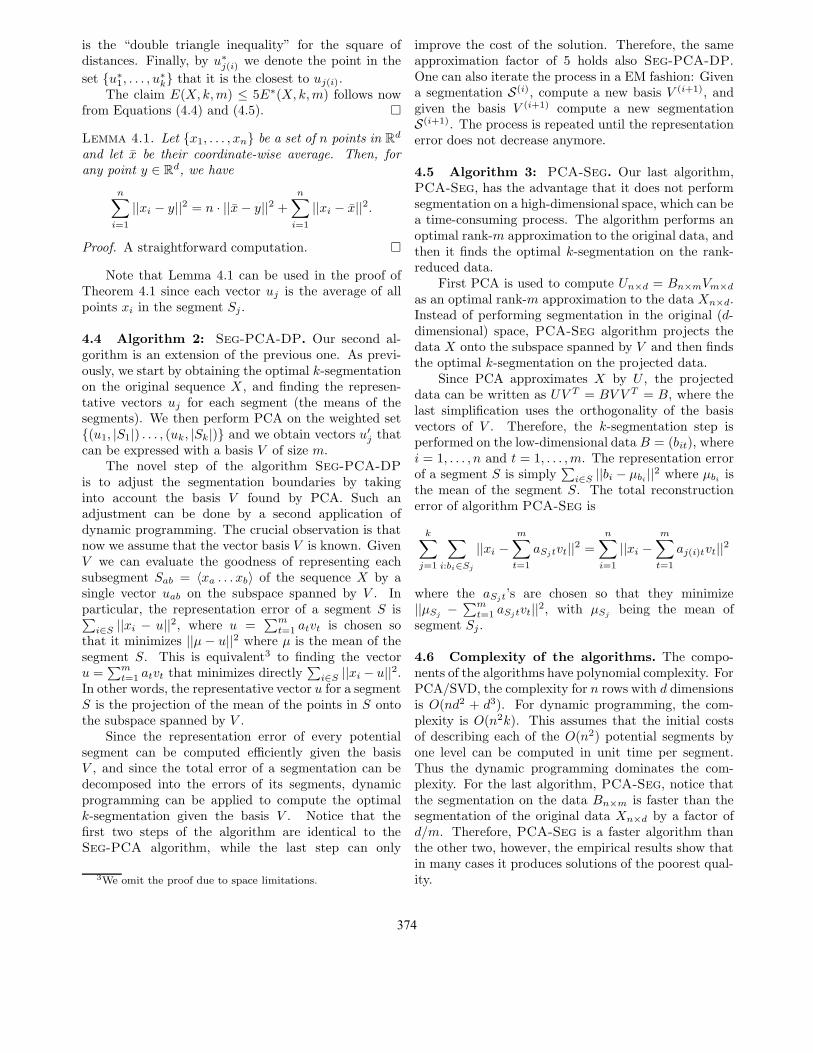
Figure 1: Basis segmentation of data on exchange rates(n = 2567, d = 12). The segment-wise coefficients ajt

for k = 20 and m = 4, algorithms Seg-PCA, Seg-

PCA-DP and PCA-Seg.

aries to the true boundaries, by measuring the sum ofdistances between the boundaries. The boundaries arerecovered almost perfectly. The sum of distances be-tween true and estimated boundaries was 10 elements(out of 1000) in the worst case (d = 20, k = 10, m =5, s = 0.25), and 0 to 2 for all datasets with s < 0.25.

5.2 Exchange rates. As a first experiment on realdata, we applied our algorithms on exchange-rate dataon 12 currencies in dollars; the 2567 observations of

1 2 3 4

AUD

BEF

CAD

FRF

DEM

JPY

NLG

NZD

ESP

SEK

CHF

GBP

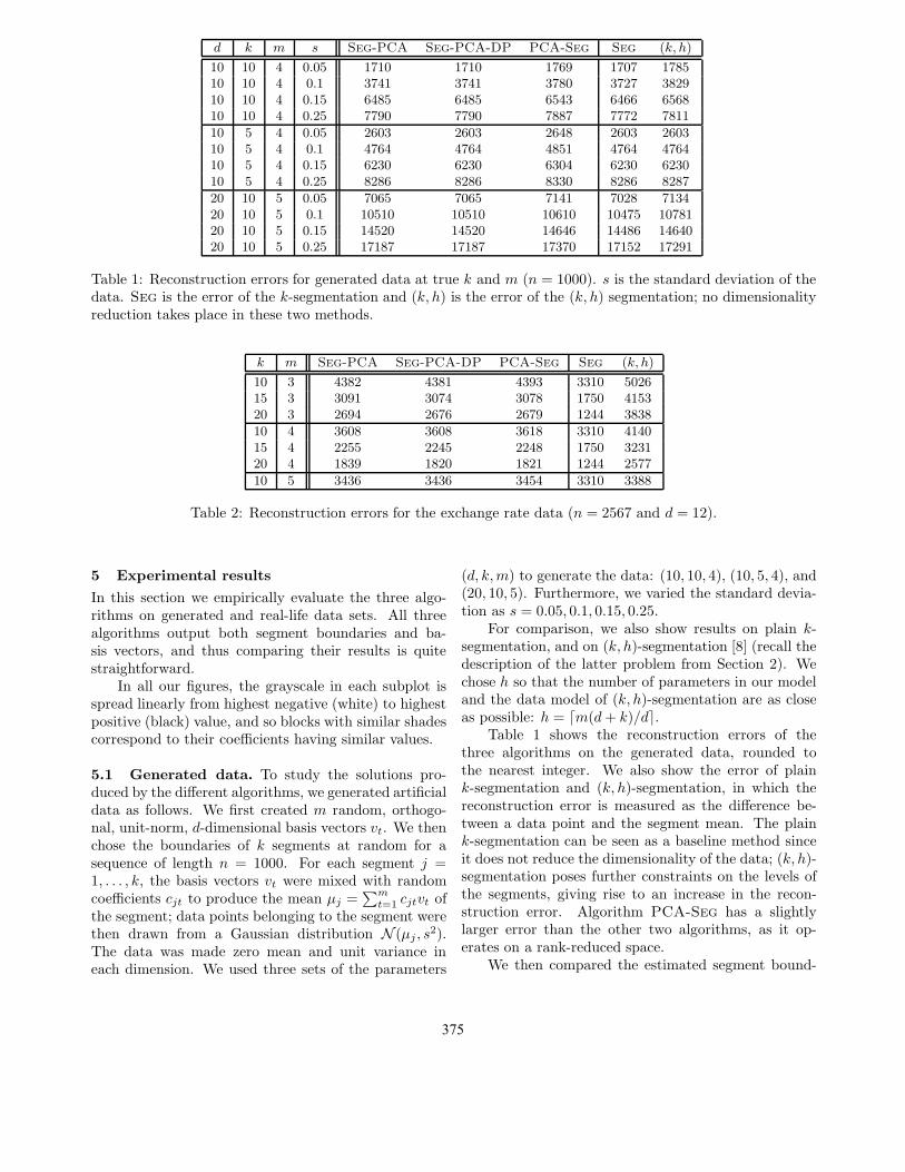
Figure 2: Basis vectors of the exchange rate dataat Algorithms Seg-PCA and Seg-PCA-DP at k =20, m = 4.

daily rates are from 1986 to 1996. The 12 currenciesare AUD, BEF, CAD, FRF, DEM, JPY, NLG, NZD,ESP, SEK, CHF and GBP. The data were made zeromean and unit variance in each dimension. The data isavailable at UCI KDD archive [11].

The segmentations found by the three algorithmsare shown in Figure 1, where parameter values k = 20and m = 4 are chosen as an example. The resultsare quite similar, and the changes in the original dataare captured nicely (remember that white is smallest,and black largest value). The reconstruction errors areshown in Table 2 for k = 10, 15, 20 and m = 3, 4, 5. Alsothe reconstruction errors have only small differences.

Figure 2 shows the basis vectors for the case k = 20and m = 4 for algorithms Seg-PCA and Seg-PCA-

DP, which use the same set of basis vectors. Thebasis vectors are ordered according to their importance.

376

k m Seg-PCA Seg-PCA-DP PCA-Seg Seg

10 2 3633 3618 3675 318110 3 3355 3355 3375 318110 4 3221 3221 3246 318110 5 3195 3195 3218 3181

15 2 3375 3237 3314 259315 3 2937 2867 2882 259315 4 2691 2691 2699 259315 5 2649 2649 2661 2593

20 2 3196 3023 3092 220520 3 2588 2534 2538 220520 4 2318 2318 2325 220520 5 2271 2271 2284 2205

25 2 3000 2923 2984 191425 3 2339 2288 2292 191425 4 2054 2051 2056 191425 5 1994 1994 1998 1914

Table 4: Reconstruction errors for human chromosome 22 + zebrafish chromosome 25 (n = 1031 and d = 16).

500 1000 1500 2000 2500−2

−1

0

1

2SEG−PCA

500 1000 1500 2000 2500−2

−1

0

1

2SEG−PCA−DP

500 1000 1500 2000 2500−2

−1

0

1

2PCA−SEG

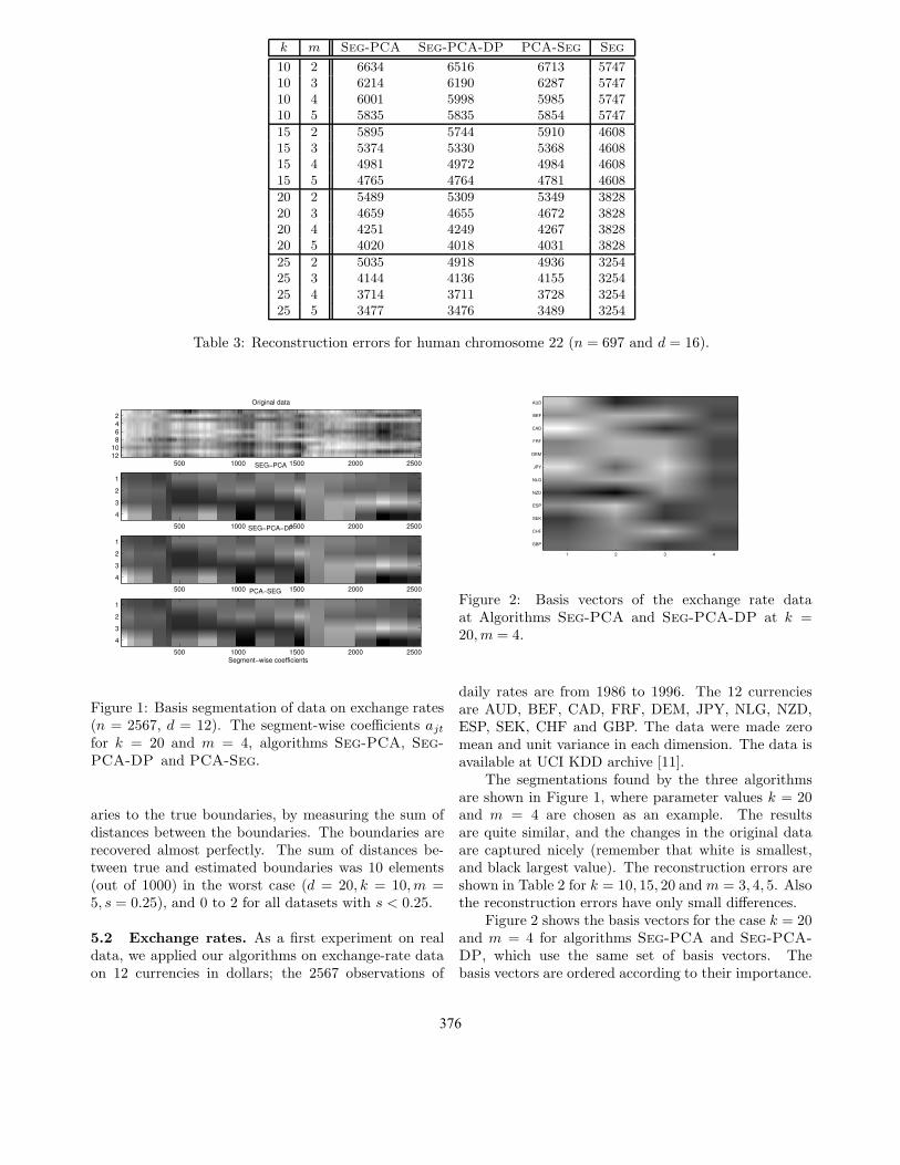
Figure 3: Segmentation on DEM of the exchange ratedata (n = 2567, d = 12) for k = 20 and m = 4,algorithms Seg-PCA, Seg-PCA-DP and PCA-Seg.

The importance of a vector is measured as the amountof variability of the data it accounts for. We seethat the first basis vector has a large negative value(light) for AUD, CAD and JPY which thus behavesimilarly, whereas SEK and NZD (dark) behave in theopposite manner. Similarly, for the second and thirdbasis vectors we can find a few extreme currencies, andthe fourth shows only minor distinctions between thecurrencies. (The basis vectors of algorithm PCA-Seg

are quite similar to those in Figure 2.) CombiningFigures 1 and 2 we see which currencies have the largest

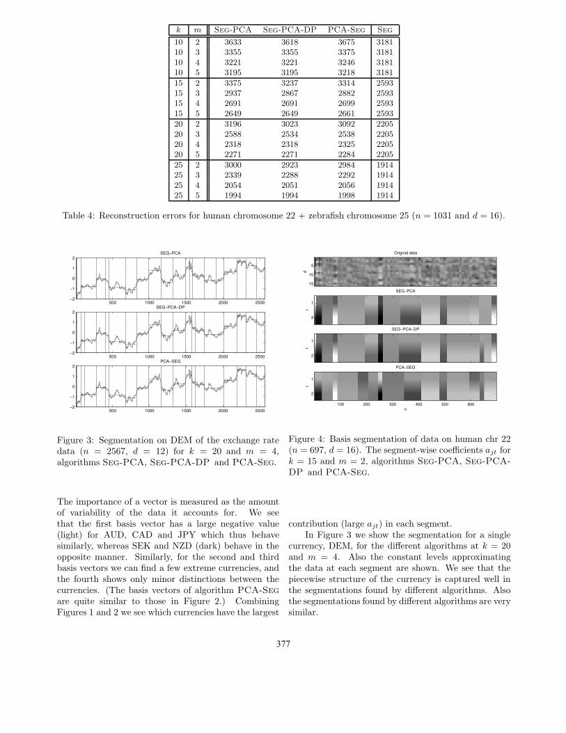
Original data

d

5

10

15

SEG−PCA

t1

2

SEG−PCA−DP

t

1

2

PCA−SEG

t

n100 200 300 400 500 600

1

2

Figure 4: Basis segmentation of data on human chr 22(n = 697, d = 16). The segment-wise coefficients ajt fork = 15 and m = 2, algorithms Seg-PCA, Seg-PCA-

DP and PCA-Seg.

contribution (large ajt) in each segment.In Figure 3 we show the segmentation for a single

currency, DEM, for the different algorithms at k = 20and m = 4. Also the constant levels approximatingthe data at each segment are shown. We see that thepiecewise structure of the currency is captured well inthe segmentations found by different algorithms. Alsothe segmentations found by different algorithms are verysimilar.

377

chr k m Seg-PCA Seg-PCA-DP PCA-Seg Seg

1 25 3 69251 69232 70201 682401 50 2 61929 61429 62960 584671 50 3 60736 60367 61092 58467

2 40 3 84640 84610 84667 826762 45 3 82443 82390 82429 80180

3 50 3 58024 57378 57389 548153 60 3 55361 54880 54963 519903 70 3 53235 52817 52915 49705

13 50 2 24229 24059 24123 2079913 50 3 22580 22450 22766 2079913 50 4 21788 21774 22651 20799

14 50 2 20483 20154 20174 1784614 50 3 19549 19362 19441 1784614 50 4 18915 18795 19263 17846

Table 5: Reconstruction errors for human chromosomes 1 (n = 2259), 2 (n = 2377), 3 (n = 1952), 13 (n = 956)and 14 (n = 882); the data consist of the frequencies of all 3-letter words, so d = 64.

k Seg-PCA Seg-PCA-DP PCA-Seg Seg (k, h)

7 9429 9429 9644 9409 940910 8545 8542 8764 8454 845415 7961 7935 8071 7684 7785

Table 6: Reconstruction errors for the El Nino data with m = 5 (n = 1480 and d = 10).

5.3 Genome sequences. Another application of ourmethod is on mining the structure of genome sequences.The existence of segments in DNA sequences is welldocumented [16, 19], and discovering a vector basiscould shed more light to the composition of the differentgenomic segments.

To demonstrate the validity of our approach we ex-perimented on small chromosomes of both human (chro-mosome 22) and zebrafish (chromosome 25). We con-verted the sequenced regions of these chromosomes intomultidimensional time series by counting frequencies of2-letter words in fixed-sized overlapping windows. Thusthe dimension of the resulting time series is d = 42 = 16.The data were normalized to have zero mean and unitvariance in each dimension separately. We used windowsize of 500 kilobase pairs (Kbp), overlapping by 50 Kbp,which resulted in 697 and 334 windows for the humanand zebrafish chromosomes, respectively.

The resulting 16-dimensional time series, as well asthe results of the different algorithms on the humanchromosome are shown in Figure 4 for k = 15 andm = 2. The corresponding basis vectors are shown inFigure 6. All the algorithms find segmentations withsimilar boundaries and similar basis vector coefficients.For instance, by observing the basis vectors one notesthat the words ‘AA’, ‘AT’, ‘TA’, ‘TT’ are described by

a similar high positive value in the second basis vector.The algorithms Seg-PCA and Seg-PCA-DP producea basis vector with high values for ‘AC’ and ‘CG’, whilePCA-Seg produces a vector with high values for ‘GT’and ‘TG’.

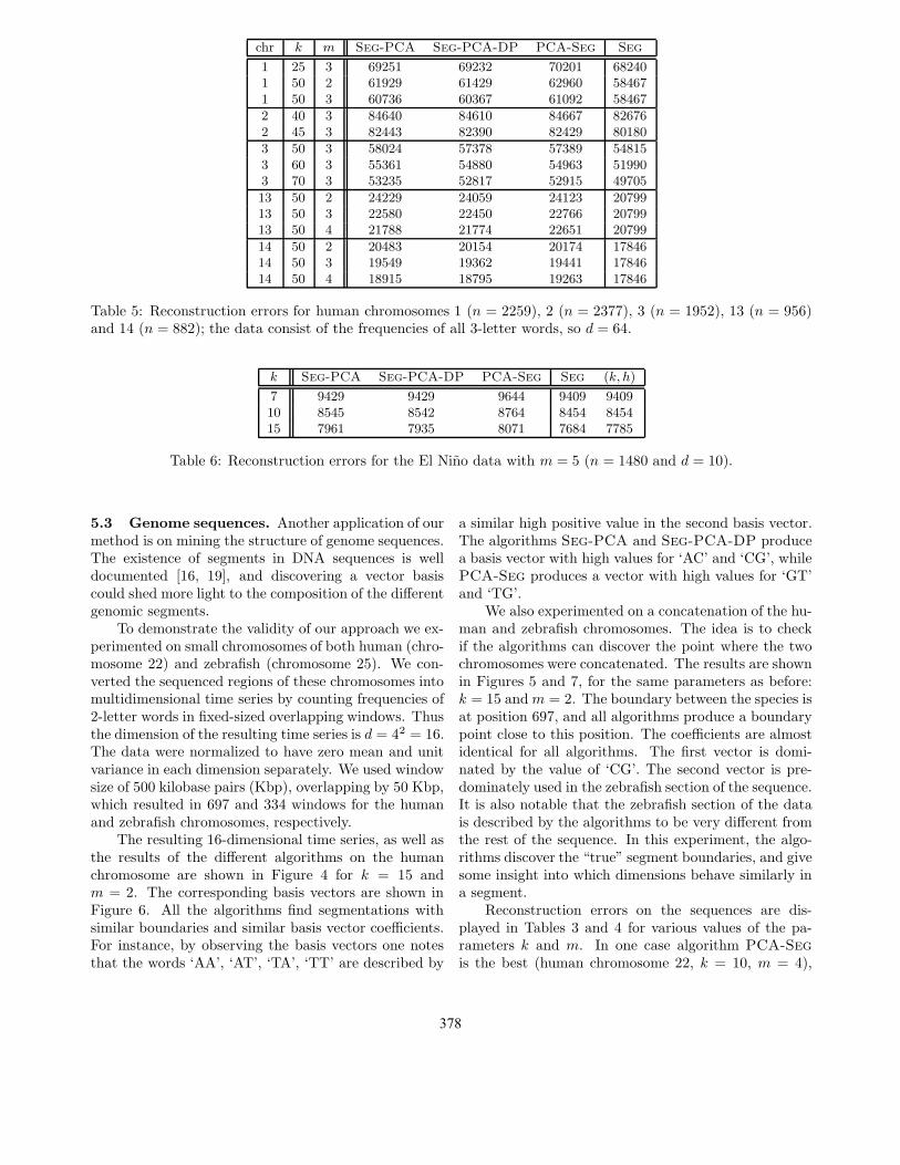
We also experimented on a concatenation of the hu-man and zebrafish chromosomes. The idea is to checkif the algorithms can discover the point where the twochromosomes were concatenated. The results are shownin Figures 5 and 7, for the same parameters as before:k = 15 and m = 2. The boundary between the species isat position 697, and all algorithms produce a boundarypoint close to this position. The coefficients are almostidentical for all algorithms. The first vector is domi-nated by the value of ‘CG’. The second vector is pre-dominately used in the zebrafish section of the sequence.It is also notable that the zebrafish section of the datais described by the algorithms to be very different fromthe rest of the sequence. In this experiment, the algo-rithms discover the “true” segment boundaries, and givesome insight into which dimensions behave similarly ina segment.

Reconstruction errors on the sequences are dis-played in Tables 3 and 4 for various values of the pa-rameters k and m. In one case algorithm PCA-Seg

is the best (human chromosome 22, k = 10, m = 4),

378

Original data

d

5

10

15

SEG−PCA

t1

2

SEG−PCA−DP

t

1

2

PCA−SEG

t

n100 200 300 400 500 600 700 800 900 1000

1

2

Figure 5: Basis segmentation of data on human chr 22+ zebrafish chr 25 (n = 1031, d = 16). The segment-wise coefficients ajt for k = 15 and m = 2, algorithmsSeg-PCA, Seg-PCA-DP and PCA-Seg. The speciesboundary is located at position 697.

but in most cases it has the largest error. AlgorithmSeg-PCA is in general very close to Seg-PCA-DP.

Finally, we experimented with human chromosomes1, 2, 3, 13 and 14. We divided the sequenced regionsof these chromosomes into nonoverlapping 100 Kbpwindows, making the number of data points much largerthan in the previous cases. In this experiment wecount the frequencies of 3-letter words in each window,producing a time series of dimension d = 43 = 64; recallthat in the previous experiments we used 2-letter wordsresulting in 16-dimensional data. Reconstruction errorsfor the long sequences of 3-letter words are displayed inTable 5. Algorithm Seg-PCA-DP is always the bestof the three algorithms, but the differences are usuallynot very large. One noteworthy feature is that m = 3or m = 4 is sufficient to get reconstruction errors veryclose to the segmentation error in the full-dimensionalspace.

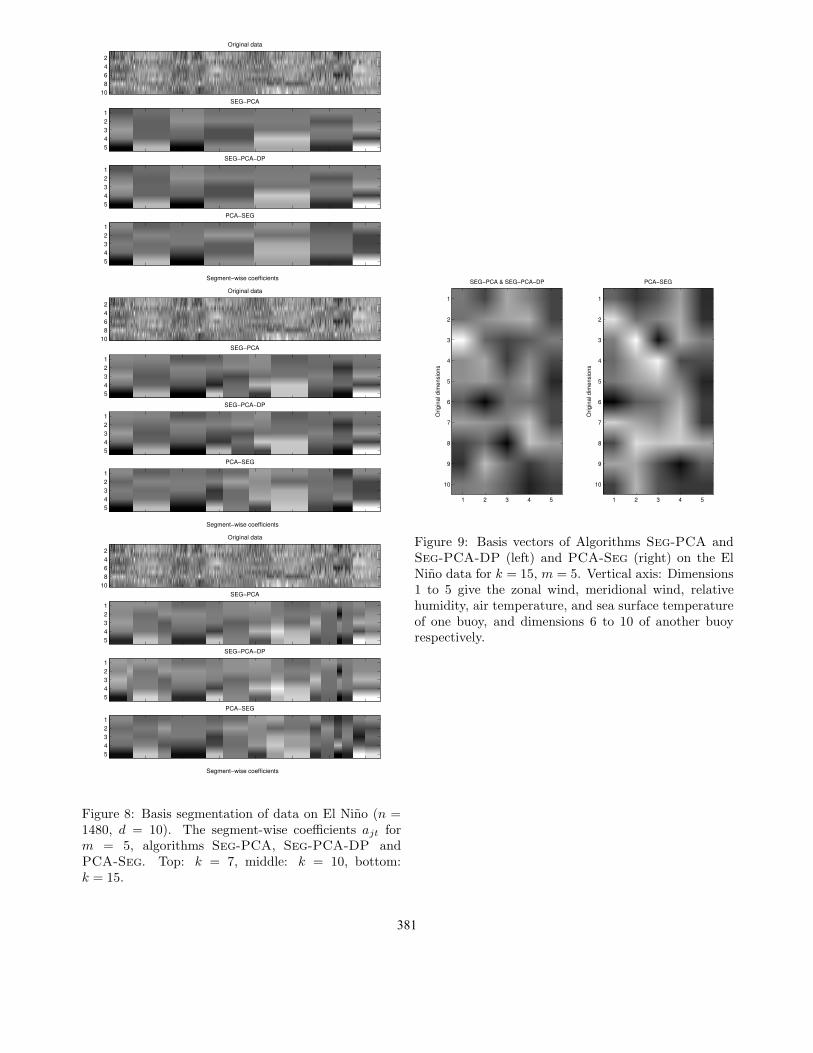
5.4 El Nino data. We also experimented on dataon El Nino [11] that contains oceanographic and sur-face meteorological readings taken from a series of buoyspositioned throughout the equatorial Pacific. We se-lected 2 buoys having 1480 common dates of measure-ments, and constructed 10-dimensional data of zonalwinds, meridional winds, relative humidity, air temper-ature, and sea surface temperature of the 2 buoys. Weselected the number of basis vectors as m = 5, corre-sponding to the number of significant eigenvalues in thecovariance matrix of the data. The data was made zero

t

SEG−PCA & SEG−PCA−DP

1 2

AA

AC

AG

AT

CA

CC

CG

CT

GA

GC

GG

GT

TA

TC

TG

TT

t

PCA−SEG

1 2

AA

AC

AG

AT

CA

CC

CG

CT

GA

GC

GG

GT

TA

TC

TG

TT

Figure 6: Basis vectors, human chr 22 (k = 15, m = 2).

mean and unit variance in each dimension separately.Table 6 shows the reconstruction errors for k = 7, 10and 15 segments.

Naturally, the error decreases as k increases. Itis evident that the reconstruction error of plain k-segmentation is quite close to that of algorithms Seg-

PCA and Seg-PCA-DP, meaning that the dimension-ality reduction from 10 to 5 does not hurt the accuracymuch.

Figure 8 shows the original data together with thesegment-wise coefficients ajt as grayscale images, foreach of the three algorithms Seg-PCA, Seg-PCA-

DPand PCA-Seg for k = 7, 10, 15. Looking at theoriginal data suggests that the block structure foundmakes sense. The segment boundaries are seen asthe change points of the coefficient values; there areslight differences between the boundaries of the threealgorithms.

To help interpreting the results of Figure 8, the basisvectors are shown in Figure 9 for k = 15; the casesat other k are quite similar. One notes that the zonaland meridional winds often behave similarly in PCA(dimensions 1 to 2, and 6 to 7), as do the air and seasurface temperatures (dimensions 4 to 5, and 9 to 10);this is not very surprising, considering the nature of thedata. Again, we can identify a few significant featuresin each basis vector as the ones having a very light orvery dark value in Figure 9.

6 Conclusions

We have introduced the basis segmentation problem,given three algorithms for it, and presented empiricalresults on their performance. The results show that the

379

t

SEG−PCA & SEG−PCA−DP

1 2

AA

AC

AG

AT

CA

CC

CG

CT

GA

GC

GG

GT

TA

TC

TG

TT

t

PCA−SEG

1 2

AA

AC

AG

AT

CA

CC

CG

CT

GA

GC

GG

GT

TA

TC

TG

TT

Figure 7: Basis vectors, human chr 22 + zebrafish chr25 (k = 15, m = 2).

Seg-PCA and Seg-PCA-DP algorithms perform verywell in practice, finding the true generating model insimulated data, and almost always yielding the smallesterrors on real data. These observations are supportedby the factor 5 approximability result. On the otherhand, algorithm PCA-Seg in general produces resultsnot too far from the other two algorithms, and is fasterby a factor of d/m.

We have also discussed experimental results on realdata that demonstrate the possible applications of ourapproach in sequence analysis; the general methodologyand problem setting can be applied in analyzing multi-dimensional time series, such as in our examples withexchange-rate data, or in bioinformatics in discoveringhidden structure in genomic sequences. A fascinatingfuture theme would be to look for possibilities of on-line segmentation and dimensionality reduction, in thespirit of [14, 9].

Several open problems still remain with respect tothe basis segmentation problem. First, what is the com-putational complexity of the problem? The componentsof the problem, segmentation and dimensionality reduc-tion, are polynomial in at least some forms, but it is notclear whether this translates to a polynomial-time solu-tion. No very simple reduction for proving NP-hardnessseems apparent.

The practical applications of the basis segmentationalgorithms are also interesting: how strong is the latentstructure in real data, i.e., do the different segmentsin some cases really have an underlying common basis?Our experiments point to this direction.

References

[1] H. Attias. Independent factor analysis with temporallystructured sources. In Advances in Neural Information

Processing Systems, volume 12. MIT Press, 2000.[2] R. K. Azad, J. S. Rao, W. Li, and R. Ramaswamy.

Simplifying the mosaic description of DNA sequences.Physical Review E, 66, article 031913, 2002.

[3] Y. Azar, A. Fiat, A. R. Karlin, F. McSherry, andJ. Saia. Spectral analysis of data. In STOC, 2001.

[4] R. Bellman. On the approximation of curves by linesegments using dynamic programming. Communica-

tions of the ACM, 4(6), 1961.[5] E. Bingham, A. Kaban, and M. Girolami. Topic

identification in dynamical text by complexity pursuit.Neural Processing Letters, 17(1):69–83, 2003.

[6] E. G. Carlstein, D. Siegmund, and H.-G. Muller.Change-Point Problems. IMS, 1994.

[7] S. C. Deerwester, S. T. Dumais, T. K. Landauer, G. W.Furnas, and R. A. Harshman. Indexing by latentsemantic analysis. Journal of the American Society of

Information Science, 41(6):391–407, 1990.[8] A. Gionis and H. Mannila. Finding recurrent sources

in sequences. In ReComB, 2003.[9] S. Guha, D. Gunopulos, and N. Koudas. Correlat-

ing synchronous and asynchronous data streams. InSIGKDD, 2003.

[10] S. Guha, N. Koudas, and K. Shim. Data-streams andhistograms. In STOC, pages 471–475, 2001.

[11] S. Hettich and S. D. Bay. The UCI KDD Archive[http://kdd.ics.uci.edu], 1999. UC, Irvine.

[12] J. Himberg, K. Korpiaho, H. Mannila, J. Tikanmaki,and H. T. Toivonen. Time series segmentation forcontext recognition in mobile devices. In ICDM, 2001.

[13] E. Keogh, K. Chakrabarti, S. Mehrotra, and M. Paz-zani. Locally adaptive dimensionality reduction for in-dexing large time series databases. In SIGMOD, 2001.

[14] E. Keogh, S. Chu, D. Hart, and M. Pazzani. Anonline algorithm for segmenting time series. In IEEE

International Conference on Data Mining, 2001.[15] M. Koivisto et al. An MDL method for finding

haplotype blocks and for estimating the strength ofhaplotype block boundaries. In Pacific Symposium on

Biocomputing, 2003.[16] W. Li. DNA segmentation as a model selection process.

In RECOMB 2001, pages 204–210, 2001.[17] J. S. Liu and C. E. Lawrence. Bayesian inference on

biopolymer models. Bioinformatics, 15(1):38–52, 1999.[18] C. H. Papadimitriou, H. Tamaki, P. Raghavan, and

S. Vempala. Latent Semantic Indexing: A ProbabilisticAnalysis. In PODS, 1998.

[19] A. Pavlicek, J. Paces, O. Clay, and G. Bernardi. Acompact view of isochores in the draft human genomesequence. FEBS Letters, 511:165–169, 2002.

[20] V. Ramensky, V. Makeev, M. Roytberg, and V. Tu-manyan. DNA segmentation through the Bayesian ap-proach. Journal of Computational Biology, 2000.

380

Original data

2468

10SEG−PCA

12345

SEG−PCA−DP

12345

Segment−wise coefficients

PCA−SEG

12345

Original data

2468

10SEG−PCA

12345

SEG−PCA−DP

12345

Segment−wise coefficients

PCA−SEG

12345

Original data

2468

10SEG−PCA

12345

SEG−PCA−DP

12345

Segment−wise coefficients

PCA−SEG

12345

Figure 8: Basis segmentation of data on El Nino (n =1480, d = 10). The segment-wise coefficients ajt form = 5, algorithms Seg-PCA, Seg-PCA-DP andPCA-Seg. Top: k = 7, middle: k = 10, bottom:k = 15.

Orig

inal

dim

ensi

ons

SEG−PCA & SEG−PCA−DP

1 2 3 4 5

1

2

3

4

5

6

7

8

9

10

Orig

inal

dim

ensi

ons

PCA−SEG

1 2 3 4 5

1

2

3

4

5

6

7

8

9

10

Figure 9: Basis vectors of Algorithms Seg-PCA andSeg-PCA-DP (left) and PCA-Seg (right) on the ElNino data for k = 15, m = 5. Vertical axis: Dimensions1 to 5 give the zonal wind, meridional wind, relativehumidity, air temperature, and sea surface temperatureof one buoy, and dimensions 6 to 10 of another buoyrespectively.

381