Sediment TIE Guidance Document - Solutions Project · sediments could prove to be very useful to...

United States Office of Research and EPA/600/R-07/080 Environmental Protection Development September 2007 Agency Washington, DC 20460

Sediment Toxicity Identification Evaluation (TIE) Phases I, II, and III Guidance Document

i

EPA/600/R-07/080

September 2007


Edited by

Kay T. Ho Robert M. Burgess

U. S. Environmental Protection Agency National Health and Environmental Effects Research Laboratory

Atlantic Ecology Division Narragansett, Rhode Island 02882

David R. Mount Teresa J. Norberg-King

J. Russell Hockett U. S. Environmental Protection Agency

National Health and Environmental Effects Research Laboratory Mid-Continent Ecology Division

Duluth, Minnesota 55804

ii

The Office of Research and Development (ORD) has produced this document to provide guidance for the identification of toxicants in sediments. These methods may be useful as a complement to existing sediment assessment tools. This document should be cited as

U.S. EPA. 2007. Sediment Toxicity Identification Evaluation (TIE) Phases I, II, and III Guidance Document EPA/600/R-07/080 Office of Research and Development. Washington, DC

This document can also be found in electronic format at the following web address: http://www.epa.gov/nheerl/publications/files/Sediment TIE Guidance Document.pdf

or http://www.epa.gov/nheerl/publications/

The information in this document has been funded wholly by the U.S. Environmental Protection Agency. It has been subject to the Agency’s peer and administrative review as document #AED-06-108, and it has been approved for publication as an EPA document. Mention of trade names or commercial products does not constitute endorsement or recommendation for use.

http://www.epa.gov/nheerl/publications/files/Sediment TIE Guidance Document.pdf

iii

Abstract Sediment contamination in the United States has been amply documented and, in order to comply with the 1972 Clean Water Act, the U.S. Environmental Protection Agency must address the issue of toxic sediments. Contaminated sediments from a number of freshwater and marine sites have demonstrated acute and/or chronic toxicity to a variety of test species, as well as adverse ecological effects such as population declines and changes in community structure. However, simply knowing that a sediment is toxic has limited use. This document provides guidance on the performance of sediment Toxicity Identification and Evaluation (TIE). TIE methods allow for the identification of toxic chemicals or chemical classes causing observed toxicity. The identification of pollutants responsible for toxicity of contaminated sediments has broad application in a number of EPA programs as the methods can be used within the total maximum daily load (TMDL) framework, to link sediment toxicity to specific dischargers, to design cost-effective remediation programs, and to identify environmentally protective options for dredged material disposal. In addition, the identification of specific problem contaminants in sediments could prove to be very useful to EPA programs involved in the development of water or sediment quality guidelines, and the registration of new products such as pesticides. Finally, knowledge of the causes of toxicity that influence ecological changes such as community structure would be useful in performing ecological risk assessments not only for the Agency but also for the scientific and regulated community as a whole. This document provides guidance for both interstitial water and whole sediment TIEs and combines our current understanding of TIE methods for both marine and freshwater interstitial waters and whole sediments. This guidance does not include approaches for the implementation of sediment TIE in a regulatory context.

This document contains Phase I TIE (characterization) methods for interstitial waters and whole sediments, including guidance on when to use whole sediment or interstitial water methods, the collection of interstitial waters for testing, and test volume considerations. Interstitial water methods include the following manipulations: graduated pH, aeration, filtration, C18 reverse-phase chromatography extraction, EDTA addition, and cation exchange solid phase extraction. Whole sediment methods include general procedures and considerations for whole sediment testing and the following manipulations: Ulva lactuca, zeolite, cation exchange resin, anion exchange resin, acid volatile sulfide, Ambersorb, and powdered coconut charcoal additions and base metal substitution. Existing guidance for Phases II and III methods have been tailored for chemical classes normally found in sediments.

iv


Acknowledgements

The following individuals have contributed technical information used in generating this guidance document.

Gerald T. Ankley U. S. Environmental Protection Agency (USEPA), National Health and Environmental Effects Research Laboratory (NHEERL), Mid-Continent Ecology Division, Duluth, MN

Robert M. Burgess USEPA, NHEERL, Atlantic Ecology Division, Narragansett, RI Joseph R. Dierkes ASci Corporation, Duluth, MN (current address: ERA Laboratories,

Duluth, MN) Larry J. Heinis USEPA, NHEERL, Mid-Continent Ecology Division Terry L. Highland USEPA, NHEERL, Mid-Continent Ecology Division Kay T. Ho USEPA, NHEERL, Atlantic Ecology Division J. Russell Hockett USEPA, NHEERL, Mid-Continent Ecology Division James Huckins U. S. Geological Survey, Columbia MO Correne T. Jenson USEPA, NHEERL, Mid-Continent Ecology Division Jon Lebo U. S. Geological Survey, Columbia MO Marta T. Lukasewycz USEPA, NHEERL, Mid-Continent Ecology Division David R. Mount USEPA, NHEERL, Mid-Continent Ecology Division Teresa J. Norberg-King USEPA, NHEERL, Mid-Continent Ecology Division Marguerite C. Pelletier USEPA, NHEERL, Atlantic Ecology Division Monique Perron Harvard School of Public Health, Harvard University, Cambridge, MA Jim Petty U. S. Geological Survey, Columbia MO Stephan A. Ryba USEPA, NHEERL, Atlantic Ecology Division Mary K. Schubauer-Berigan ASci Corporation, Duluth, MN (current address: NIOSH, Cincinnati, OH) Jonathan R. Serbst USEPA, NHEERL, Atlantic Ecology Division Carol A. Shreve Senior Service America, Inc., Duluth, MN

Editorial Assistance Production Assistance Mary Keane Patricia DeCastro Consulting Editor Computer Sciences Corporation Wakefield, RI Narragansett, RI

Special Acknowledgment to the numerous contributors to USEPA’s freshwater sediment porewater

methods guidance (USEPA 1992a)

v

Contents

Abstract ................................................................................................................................ iii

Abbreviations ....................................................................................................................... x

1 Introduction.......................................................................................................................... 1 1.1 Background ................................................................................................................... 1 1.2 The TIE Concept........................................................................................................... 2 1.3 The TIE Approach for Sediments ................................................................................. 3 1.4 Document Organization ................................................................................................ 4

2 Health and Safety................................................................................................................. 5

3 Quality Assurance................................................................................................................ 6 3.1 TIE Quality Control Plans ............................................................................................ 6 3.2 Cost Considerations and Concessions .......................................................................... 6 3.3 Variability ..................................................................................................................... 7 _Toc1779681513.4 Intralaboratory Communication............................................................ 7 3.5 Record Keeping ............................................................................................................ 7 3.6 Phase I Considerations.................................................................................................. 7 3.7 Phase II Considerations................................................................................................. 9 3.8 Phase III Considerations ............................................................................................... 9

4 Equipment, Supplies, and Facilities ................................................................................. 10

5 Statistical Methods............................................................................................................. 11

6 Designing the TIE Approach ............................................................................................ 12 6.1 Defining the Question ................................................................................................. 12 6.2 Whole Sediment Versus Interstitial Water Approaches ............................................. 12 6.2.1 Comparison of Whole Sediment and IW Toxicity Tests ................................... 13 6.2.2 Selecting Whole Sediment or IW Methods for Phase I TIE.............................. 15 6.3 Species Selection for Sediment TIE ........................................................................... 17 6.4 General Considerations for Testing ............................................................................ 20

7 Phase I Overview and Methods: Whole Sediments ........................................................ 21 7.1 Toxicity Testing for Solid Phase TIE: General Procedures........................................ 21 7.1.1 Marine Test Methods ......................................................................................... 23 7.1.2 Freshwater Test Methods................................................................................... 23 7.1.3 Replication ......................................................................................................... 24 7.1.4 Controls and Procedural Blanks......................................................................... 25 7.2 Whole Sediment TIE Methods.................................................................................... 25 7.2.1 Initial Toxicity Tests .......................................................................................... 27 7.2.2 Baseline Toxicity Test ....................................................................................... 30

vi

7.2.3 Manipulations Addressing Ammonia ................................................................ 30 7.2.3.1 Algae (Ulva lactuca) Addition............................................................ 31 7.2.3.2 Zeolite Addition .................................................................................. 32 7.2.4 Manipulations Addressing Cationic Metals....................................................... 34 7.2.4.1 Cation Exchange Resin Addition........................................................ 35 7.2.4.2 Sulfide Addition.................................................................................. 36 7.2.5 Organic Toxicants.............................................................................................. 39 7.2.5.1 Coconut Charcoal Addition ................................................................ 41 7.2.5.2 Carbonaceous Resin Addition............................................................. 45 7.2.6 Whole Sediment Dilution Blank Test ................................................................ 47 7.2.7 Other Forms of Carbon Addition....................................................................... 48

8 Phase I Overview and Methods: Interstitial Water........................................................ 49 8.1 Interstitial Water Toxicity Test Procedures ................................................................ 50

8.1.1 Test Chambers ................................................................................................... 51 8.1.2 Test Design ........................................................................................................ 51 8.1.3 Volume Considerations...................................................................................... 51

8.2 Test Conditions and Physical/Chemical Monitoring .................................................. 52 8.2.1 Temperature ....................................................................................................... 53 8.2.2 Dissolved Oxygen.............................................................................................. 53

8.2.3 pH ...................................................................................................................... 53 8.2.4 Salinity ............................................................................................................... 53 8.2.5 Conductivity, Hardness, Alkalinity.................................................................... 53 8.2.6 Dilutions, Dilution Water................................................................................... 54 8.2.7 Replication ......................................................................................................... 54

8.2.8 Observations ...................................................................................................... 54 8.2.9 Feeding ............................................................................................................. 54 8.2.10Simultaneous Testing........................................................................................ 54 8.3 Initial Tests.................................................................................................................. 55

8.3.1 Baseline Test ...................................................................................................... 55 8.3.2 Volatile Compounds: Aeration .......................................................................... 56 8.3.3 Organic Compounds: Reverse-phase Solid-phase Chromatography................. 57 8.3.4 Cationic Metals: EDTA Test ............................................................................. 60 8.3.5 Graduated pH Manipulation .............................................................................. 61

8.3.5.1 Carbon Dioxide Method ..................................................................... 65 8.3.5.2 Closed-cup Method............................................................................. 69 8.3.5.3 Buffer Method..................................................................................... 70

8.3.6 Ammonia Manipulations: Ulva lactuca and Zeolite.......................................... 72 8.3.6.1 Ulva lactuca ........................................................................................ 72 8.3.6.2 Zeolite Column ................................................................................... 73

vii

9 Phase II Sediment TIE Methods for Interstitial Water and Whole Sediments ........... 74 9.1 Ammonia..................................................................................................................... 74 9.2 Cationic Metals ........................................................................................................... 77

9.2.1 Direct Chemical Analysis .................................................................................. 77 9.2.2 Zero Valent Magnesium Test............................................................................. 79 9.2.3 Species Sensitivity ............................................................................................. 82 9.2.4 Complementary Phase I Manipulations ............................................................. 82 9.2.5 Sodium Thiosulfate Test .................................................................................... 82 9.2.6 Cation Exchange Treatment of Interstitial Water .............................................. 83 9.2.7 Cation Resin Elution.......................................................................................... 84

9.3 Organic Compounds ................................................................................................... 84 9.3.1 SPMD Method for Solid-Phase Sediments........................................................ 86 9.3.2 Alternate Phase II Solid-phase Methods for Organic Compounds.................... 90 9.3.3 C18 Solid Phase Chromatography and Fractionation for Interstitial Water ....... 91 9.3.4 C18 Fractionation Considerations....................................................................... 94

9.4 Sulfide ...................................................................................................................... 94 9.5 Toxicity Caused by Major Cations and Anions.......................................................... 96 9.6 Manipulations Addressing Selected Anionic Metals: Chromium and Arsenic .......... 97 9.7 Phase II Approaches When No Phase I Manipulations Affect Toxicity .................. 100 9.8 Manipulations Under Acidic and Basic Conditions.................................................. 103

9.8.1 Aeration ........................................................................................................... 104 9.8.2 C18 Reverse-phase Solid-phase Chromatography............................................ 105

9.9 Phase II Summary..................................................................................................... 105

10 Phase III Sediment TIE Methods ................................................................................... 107 10.1 Defining the Objectives of Phase III......................................................................... 107 10.2 Solid-Phase Versus Interstitial Water Testing .......................................................... 108 10.3 Predicting Chemical Toxicity in Sediments ............................................................. 109 10.4 Correlation ................................................................................................................ 110 10.5 Spiking .................................................................................................................... 113 10.6 Species Sensitivity .................................................................................................... 117 10.7 Symptoms ................................................................................................................. 119 10.8 Matrix Changes......................................................................................................... 119 10.9 Phase III Summary.................................................................................................... 120

Literature Cited ........................................................................................................................ 121

viii v

Figures Figure 7–1 TIE Approach with Whole Sediments ................................................................. 26 Figure 7–2 Effect of Sulfide Addition on the Toxicity of Metal-spiked Sediments to H. azteca

and C. dilutus ....................................................................................................... 39 Figure 7–3 Sublethal Response of H. azteca and C. dilutus to Different Particle Sizes and

Addition Rates of Coconut Charcoal to an Uncontaminated Sediment ............... 42 Figure 7–4 Reduction in Concentration of Individual PCB Congeners in the Interstitial Water

of a Field-collected Sediment Following Treatment with 4% Ambersorb 1500 433 Figure 7–5 Response of H. azteca and C. dilutus to a Field Sediment Contaminated with

DDT and a Clean Sediment Spiked with Dieldrin................................................ 44 Figure 7–6 Effectiveness of Different Ambersorb Resins and Addition Rates on the Response

of C. dilutus Exposed to Dieldrin-spiked Sediment ............................................. 45 Figure 7–7 Results of Sand Dilution Blank Test..................................................................... 48 Figure 8–1 Overview, Phase I Interstitial Water Characterization Tests ................................ 49 Figure 8–2 Change in Relative Ammonia Concentrations with Change in pH for Selected

Temperatures......................................................................................................... 62 Figure 9–1 Racks for Working with SPMDs. (a) Freshwater Stainless Steel Rack, and (b)

Marine Glass Rack................................................................................................ 89 Figure 10–1 Correlation of Concentrations of Ammonia in Sediment Interstitial Waters from

the Lower Fox River/Green Bay Watershed, with Toxicity of the Samples to Fathead Minnows and C. dubia .......................................................................... 112

ix

Tables Table 6–1 Comparison of Interstitial Water and Whole Sediment Tests (% Survival) ......... 13 Table 6–2 Commonly Used Species in the Conduct of Interstitial and Whole Sediment

Toxicity Identification Evaluations....................................................................... 18 Table 7–1 Effectiveness of Powdered Coconut Charcoal and Ambersorb in Removing

Toxicity from Spiked and Field Contaminated Sediments (% Survival) ............. 40 Table 8–1 Estimated Volumes for Phase I Interstitial Water TIE Tests ................................ 52 Table 8–2 Species Sensitivity to Phase I Additives............................................................... 59 Table 8–3 Relative Sensitivity (EC50) of Benthic and Water Column Test Species to

Different Toxicants ............................................................................................... 63 Table 8–4 Trends in Metal and Ammonia Toxicity with Respect to Test pH....................... 64 Table 8–5 Sensitivities of C. dubia, P. promelas, H. azteca, and L. variegatus to the pH-

Control Buffers, MES, MOPS, and POPSO......................................................... 71 Table 8–6 Sensitivity of C. dubia to Lead, Copper, and Zinc ............................................... 72 Table 9–1 Summary of Analytical Methods Currently Used or Proposed for Phase II TIEs 75 Table 9–2 Results of Toxicity Tests from Sediments with and Without the Base Metal

Magnesium Added (% Survivial) ......................................................................... 81 Table 9–3 Thought Experiment Demonstrating Changes in Toxic Potency Associated with

Direct Testing of Sediment Extracts ..................................................................... 85 Table 9–4 Composition of Nine Recommended Solvents and Water Combinations for

Eluting the C18 Column in Phase II Sediment TIE ............................................... 91 Table 9–5 The Effect of Graduated pH, Sodium Thiosulfate, and EDTA on Ammonia,

Copper, Lead, and Zinc Toxicity ........................................................................ 103 Table 10–1 Comparison of the Sensitivities of C. dubia, P. promelas, and P. phosphoreum to

Interstitial Water at Green Bay/Fox River .......................................................... 118 Table 10–2 Comparison of the Sensitivities of C. dubia, P. promelas, and H. azteca to

Sediment Interstitial Water from Five Sites Along Turkey Creek, Joplin, MO . 118

x

Abbreviations AED Atlantic Ecology Division, USEPA,

Narragansett, RI AET apparent effects threshold AVS acid-volatile sulfide DI deionized (water) DO dissolved oxygen EC electron capture EC50 median effective concentration

(concentration for which the endpoint is reached in 50% of the organisms)

EDTA ethylene diamine tetraacetic acid EqP equilibrium partitioning ERL effects range low ERM effect range medium ESB equilibrium partitioning sediment

benchmark fOC fraction organic carbon (usually sediment

dry weight) GC gas chromatography HPLC high performance liquid chromatography ICP inductively coupled plasma emission

spectroscopy IW interstitial water (porewater) KOC organic carbon normalized partition

coefficient

KOW octanol water partition coefficient KSPMD water SPMD partition coefficient LC liquid chromatography LC50 median lethal concentration

(concentration that kills 50% of the organisms)

MED Mid-Continent Ecology Division, USEPA, Duluth, MN

MEOH HPLC grade methanol MS mass spectroscopy NEC no-effect concentration NPDES National Pollution Discharge

Elimination System PAH polycyclic aromatic hydrocarbons PCBs polychlorinated biphenyls PEC probable effects concentration PEL probable effects level pHi initial pH SPE solid phase exchange SPMD semipermeable membrane device SQG sediment quality guidelines TIE toxicity identification evaluation TEL threshold effects level TOC total organic carbon

1

1 Introduction Toxicity testing is an excellent tool for monitoring sediment contamination, as it can detect the presence of both known and unknown sediment contaminants if they are present at concentrations sufficient to cause toxicity to the test organisms. The existence of sediment contamination in the United States has been documented (Long et al. 2001; USEPA 2004). To comply with the Clean Water Act, the Comprehensive Environmental Response, Compensation, and Liability Act, and other mandates, the U.S. Environmental Protection Agency (USEPA) must develop means to assess and manage ecological risks from contaminated sediments.

1.1 Background Toxicity testing of sediments from many monitoring and assessment efforts has shown that sediments from a great number of freshwater and marine sites are acutely or chronically toxic to benthic organisms (Hyland et al. 1999; USEPA 2004). Toxicity of sediments has been shown to be associated with adverse ecological effects such as population declines and changes in community structure (Anderson et al. 1987; Bailey et al. 1995; Hartwell et al. 1997; Hatakeyama and Yokoyama 1997; Swartz et al. 1994; Swartz et al. 1982). While the presence of sediment toxicity can be a strong indicator of potential ecological risk from sediment contamination, toxicity tests alone do not indicate the cause of toxicity. While the presence of toxicity alone may be sufficient for some environmental management decisions, the most effective and cost-efficient management decisions are possible when the exact cause(s) of sediment toxicity is known. Clearly, the selection of appropriate management alternatives could be altered if one knew that the cause of toxicity in a particular sediment was ammonia, as compared to DDT or zinc. As another example, in complex systems there may be a variety of sources for sediment contamination, both point (e.g., wastewater discharges) and non-point (e.g., stormwater runoff). While finding that sediments are toxic may suggest the need for better management of contamination sources, knowing the specific chemical(s) causing sediment toxicity enables more accurate definition of the source(s), and thereby focuses remedial actions on those sources contributing most directly to degradation of the sediments. For these reasons, the development of methods to link the existence of sediment toxicity to the specific cause(s) of that toxicity would be of great benefit to programs charged with managing sediment quality. One approach to identifying potential causes of sediment toxicity is chemical screening, such as priority pollutant analyses, and either comparison of those results with numerical benchmarks for sediment contamination, or correlation of measured concentration with observed toxicity. These approaches are often unsuccessful for a number of reasons:

• Presence of unmeasured chemicals While common chemical screens may detect dozens or even hundreds of chemicals, there are literally thousands of chemicals released into waterways, leaving many potential toxicants unmeasured. To rely solely on standard chemical screens is like “looking for your car keys only under the lamppost.”

• Co-correlation of sediment contaminants Because most sources of sediment contamination do not release single chemicals but rather whole suites of chemicals, concentrations of many sediment contaminants are highly correlated with others. Accordingly, correlation of sediment toxicity with chemical concentration often identifies

2

many associations that are not causal and, therefore, may provide a poor basis for environmental management decisions.

• Differences in bioavailability Even if all possible contaminants of concern could be measured, the factors that control biological availability of those chemicals to sediment organisms are not known for all chemicals and/or all sediments, leading to difficulty in defining, a priori, the concentration of a chemical that would be expected to cause adverse effects.

• Mixtures Even if all of these issues could be resolved, predicting toxicity solely from chemical concentrations would require sufficient understanding to predict the interactive toxicity of the mixtures of chemicals present.

These same problems were encountered in the National Pollutant Discharge Elimination System (NPDES) permitting program when it focused on utilizing toxicity to aquatic organisms in effluent permit limits. In response, the USEPA Office of Research and Development, specifically the ecology divisions in Duluth, MN, and Narragansett, RI, developed a biologically-based rigorous fractionation approach to identify the cause of toxicity in aqueous samples such as effluents and receiving waters (USEPA 1989a; 1991a; 1991b; 1992b; 1993a; 1996). These procedures, called a Toxicity Identification Evaluation (TIE) relied on combinations of physical/chemical manipulations and toxicity tests to characterize, identify, and confirm the causes of measured toxicity. Application of these methods through the NPDES program and others have shown them to be highly effective in determining the cause of toxicity in effluents, and an invaluable tool in the cost-effective control of effluent toxicity. This document presents TIE methods developed for application to toxic sediments. While similar in concept to the approaches developed previously for water column (e.g., effluent and receiving water) toxicity, these methods address the unique issues posed by identifying toxicants in a sediment matrix.

1.2 The TIE Concept

The basic concept in TIE or other biologically-directed fractionation approaches is to use physical/chemical manipulation of a sample to isolate or change the potency of different groups of toxicants potentially present in a sample. Rather than using a chemical detector to determine whether a change occurred, a biological test, in this case a toxicity test, is used as the “indicator” to determine whether the manipulation changed toxicity. For example, imagine taking a toxic water sample, splitting it into two aliquots, one of which is aerated and one not. If toxicity testing of these samples showed that the aerated sample was markedly less toxic than the unmanipulated sample, one might suspect that the causative toxicant is volatile or easily oxidized. By simultaneously conducting tests using multiple manipulations targeted at different physical/chemical properties, one can build a physical/chemical characterization of the toxicant(s), which in turn becomes the basis for additional studies to isolate and ultimately identify the specific chemicals causing toxicity. In developing TIE procedures for aquatic toxicity in effluents and other waters, USEPA divided the overall TIE process into three phases: characterization (Phase I), identification (Phase II), and confirmation (Phase III). While sharing many of the same concepts and general procedures, each Phase has a different goal.

3

• In Phase I, a suite of physical/chemical manipulations is used to build a general “profile” of the causative toxicant(s), with the goal of determining the general category or type of toxicant involved (e.g., metals, nonpolar organics, volatiles, ammonia).

• In Phase II, more refined procedures are used, to focus on the specific category of chemical implicated in Phase I, with the goal of isolating the causative toxicant(s) from other chemicals in the sample, thereby simplifying the sample for chemical analysis. This process generally culminates in the analytical identification of the suspected toxicant.

• In Phase III, the investigator collects the corroborating data to build a weight-of-evidence case that the suspect toxicant is in fact the cause of toxicity, an important step before initiating management actions to control the problem chemicals.

1.3 The TIE Approach for Sediments This document describes TIE procedures that have been developed for identifying the cause(s) of toxicity in sediments. While our experience in developing TIE procedures for water column toxicity formed an important basis for sediment TIE, working with sediments presented some unique challenges that required the modification of some prior procedures as well as the development of new procedures. The reader should be aware that this document was not prepared to be stand-alone guidance for conducting sediment TIEs. Because these procedures build on previous methods developed for toxicity in effluents and other water samples, we assume that the reader of this document already has a strong familiarity with those previously developed procedures. Much of the philosophy, procedures, design considerations, and interpretation issues already described are directly applicable to sediment TIE, and therefore not all repeated in this document. Investigators not already familiar with previous TIE guidance should read that previous guidance (USEPA 1989a; 1991a; 1991b; 1992b; 1993a; 1996). In keeping with previous guidance, sediment TIE has been structured around the same three elements: characterization (Phase I), identification (Phase II), and confirmation (Phase III). A complicating factor for sediments is that sediment toxicity can and has been assessed using more than one test matrix. Whole sediment exposures involve test chambers containing both a sediment layer and an overlying water layer, similar to the situation for a bedded sediment in the field. However, sediment toxicity can also be assessed using water column tests conducted on aqueous samples prepared from sediments; the most common of these is interstitial water (IW; sometimes called porewater) testing, in which water from the interstices of the sediments is isolated by centrifugation or other methods, then used in water column toxicity tests. Although IW tests are probably the most common water column tests conducted to assess sediment toxicity, there are other methods, such as the preparation of elutriates and solvent extracts. For clarity, this document refers to water column testing as IW testing since it is the most common approach, but we recognize that other water preparations might be used and expect that the guidance provided here is fully applicable in some but not all of these other instances (i.e., solvent extracts).

Another difference between this and previous TIE guidance is that procedures for both freshwater and marine TIEs have been combined into a single guidance document. We have found that the bulk of the approaches developed are equally applicable to both freshwater and marine sediments and organisms, though where differences exist we have tried to make those clear. In some cases this leads

4

to some redundancy, but we believe these are outweighed by the overall benefits of having one consolidated guidance document. The procedures we describe are not the only ones that can be used to identify toxicants in sediments. Much of what we describe are methods that we have found to be effective, but the degree to which we have explored alternatives varies. For some methods, we have spent considerable time optimizing a particular method; for others, we have not conducted sufficient studies on all the alternatives to state that the suggested method is the only, or even the best, procedure that could be used. In some cases, we suggest possible procedures that we have not actually used because we haven’t had the need, but we believe that they would work should the necessity arise. While this argues toward openness and flexibility in the procedures, we also recognize that guidance that is largely conceptual and does not contain specific procedures may be difficult to implement by laboratories new to these techniques. Toward this end, we have tried to do both: not only to provide suggested, or “default,” procedures that we believe are robust, but also to include supplementary information on the rationale behind our suggestions and perhaps alternatives that we have tried that may not have been effective. To help in this communication we have tried to use words like must, should, can, may, and might in ways consistent with their ASTM usage (ASTM 2005). It is very important to recognize that this manual represents guidance, not a strict protocol. TIEs are by nature unique investigations that may have many alternative paths that could be successfully followed to the same conclusion. The quality of a TIE lies only partially in the technical quality of the data; the more important element is the soundness of the reasoning and the creativity of the investigator. Treatment of this manual as an inviolable protocol is not recommended, and might actually be counterproductive to the overall goal of efficiently identifying toxicants.

1.4 Document Organization The remainder of this document outlines procedures for conducting sediment TIEs. General information concerning Health and Safety; Quality Assurance; Equipment, Supplies, and Facilities; and Statistical Methods are described in Sections 2 through 5. Section 6 discusses overall issues involved in designing the TIE approach, including selecting the test matrix, and procedures and species to be used, and provides recommendations for how to collect and prepare samples for sediment TIE testing, including the collection of IW. Phase I, characterization methods for whole sediment and IW, are described separately in Sections 7 and 8, respectively. Because both whole sediment and IW approaches may be used in later phases of the TIE, they are described jointly for Phase II, identification (Section 9), and Phase III, confirmation (Section 10) studies. Published studies and existing guidance are cited throughout this document when possible. Original data developed for this document are also included with appropriate documentation of materials and methods.

5

2 Health and Safety This section has been reprinted, with minor modifications, from Methods for Aquatic Toxicity Identification Evaluations: Phase I. Toxicity Characterization Procedures, Second edition (USEPA 1991b). Sediments are repositories for a wide range of chemical and biological agents. Sediment TIEs involve, by definition, working with samples of unknown composition. Therefore, the safety measures must be adequate for a wide spectrum of hazardous materials. Exposure to sediment samples during collection and in the laboratory should be kept to a minimum. Inhalation and dermal absorption can be reduced by using laboratory hoods and wearing protective gloves, laboratory aprons or coats, safety glasses, and respirators. Further guidance on health and safety for toxicity testing is described in Walters and Jameson (1984). In addition to the precautions taken with sediment samples, a number of the reagents that might be used during the tests described in this guidance are known or suspected to be toxic to people. Analysts need to be familiar with safe handling procedures for these chemicals (Occupational Safety and Health Administration 1976; U. S. Department of HEW 1977) as well as the manufacturer’s Materials Safety Data Sheets (MSDS). Use of the compounds may also necessitate specific waste disposal practices. See USEPA (2000), sections 5.1.3, 5.1.4, 5.2, 5.3, 5.4 and 5.5 for more information.

6

3 Quality Assurance The following section has been reprinted, with minor modifications, from Methods for Aquatic Toxicity Identification Evaluations: Phase I Toxicity Characterization Procedures, Second edition (USEPA 1991b).

Quality assurance comprises two aspects: quality verification and quality control. Quality verification entails a demonstration that the proposed study plan was followed as detailed and that work carried out was properly documented. Aspects of quality verification include chain-of-custody procedures, statements on the objective of the study and what is known about the problem at its outset, instrumental log books, and work assignments. This aspect of quality assurance ensures that documentation is created to prove that the work plan has been covered completely. The quality control aspect of quality assurance involves the procedures that take place, such as the number of samples to be taken and the mode of collection, standard operating procedures for analyses, and spiking protocols.

3.1 TIE Quality Control Plans A successful TIE depends on a strong quality control program. Obtaining quality TIE data is complex because the constituents are unknown, in contrast to obtaining quality data from a standard analytical method for a specific chemical, where the characteristics of the analyte and the implications of the analytical procedure being used are known. Without knowledge of the physical and chemical characteristics of the analyte, however, the impact of various analytical procedures on the compound under study is not known. Further, quality control procedures are specific to each compound. Quality control procedures appropriate to one analyte might be completely inappropriate to another. Because TIEs use both chemical and biological assays, the problem of quality control is further aggravated because quality control procedures for aquatic toxicity tests might be radically different from those required for individual chemical analyses. This additional dimension to quality control requires a unique framework of checks and controls to be successful. The impacts of chemical analytical procedures on sample toxicity must be included. Likewise, procedures used to insure quality toxicity test results should not affect chemical analyses. For example, in a standard aquatic toxicity test, samples with low dissolved oxygen (DO) are usually aerated. This practice might, however, result in a loss of toxicity if the toxicant is volatile or subject to oxidation. Given the multidisciplinary complexities of this work, it is recommended that quality control plans are supported by standard operating procedures (SOPs).

3.2 Cost Considerations and Concessions The quality control practices required in any given experiment must be weighed against the importance of the data and decisions to be based on that data. The crucial nature of certain data demands stringent controls, while quality control can be lessened in other experiments having less impact on the overall outcome. Sediment TIEs require a large number of toxicity tests and a good deal of interstitial water. In interstitial waters, the decision to use the standard toxicity test methods described in USEPA (1995; 2000; 2001; 2002a; 2002b) which involved a relatively high degree of quality control,

7

must be weighed against the degree of complexity involved, the time required, and number of tests performed. All of these contingencies affect the cost of testing. In addition, obtaining large volumes of interstitial water can be labor intensive and time consuming. For this reason, replication and size of toxicity tests are both minimized.

3.3 Variability In retesting sediments to confirm the quality of initial TIE results, possible sources of error need to be considered, including changes in the chemical and toxicological nature of the sediments over time in storage or in the field. Changing field conditions may alter salinity, pH, and redox potential of sediments, which, in turn, might influence the toxicity of metals, ammonia, and hydrogen sulfide. Also, patchiness in the field might limit the ability to obtain the same or similar sediments.

While studies vary in their recommendations (Beiras et al. 1998; Carr and Chapman 1995; DeFoe and Ankley 1998; Dillon et al. 1994; Ho and Quinn 1993; Malueg et al. 1986; Othoudt et al. 1991; Thompson et al. 1980), we have successfully used sediments stored up to three years to reconfirm initial findings of sediment TIEs. Caveats include being aware that certain volatile compounds such as ammonia and hydrogen sulfide may decrease in concentration, and changes in redox potential might affect the toxicity of metals and other ionizable compounds. If particularly volatile or unstable toxicants are suspected, it may be necessary to test freshly collected sediments.

3.4 Intralaboratory Communication Quality control procedures can be quite different for chemistry and biology. For example, phthalates are a frequent analytical contaminant requiring special precautions that are not of toxicological concern. The toxicological problem presented by zinc levels typically associated with new glassware is of no concern to organic analysis. The difference in glassware cleanup procedures is an example of one of many differences that must be resolved when working among different disciplines in a laboratory. Cleaning procedures must be established to cover the requirements of all of the involved disciplines. Time schedules for analyses must be detailed in advance to avoid delays that may change toxicant concentrations and effects. Frequent, well documented, communication of a well designed experiment involving all concerned parties is one of the keys to performing successful TIEs.

3.5 Record Keeping Throughout the TIE, record keeping is an important aspect of quality verification. All observations, including organism symptoms, should be documented. Details that seem unimportant during testing can be crucial in later stages of the evaluation. Investigators should record test results in such a manner that preconceived notions about the sediment toxicants are not unintentially reflected in the data.

3.6 Phase I Considerations Sediment toxicity is “tracked” through Phases I, II, and III using aquatic or benthic organisms. Such tracking is the only way to detect where the toxicants are until their identity is known. The organism’s response must be considered as the foundation. Therefore, the toxicity test results

8

must be dependable. System blanks (blank samples carried through procedures and analyses identical to those performed on effluent samples) are critical to the process and are used extensively throughout the TIE to detect toxic artifacts added during the sediment characterization manipulations. With the exception of tests intended to make the sample more toxic, or cases in which a known amount of toxicity has been intentionally added, TIE manipulation should not cause the sample toxicity to increase. There are many sources of toxicity artifacts in Phase I. These include • Excessive ionic strength resulting from the addition of acid and base during pH adjustment • Formation of toxic products by acids and bases • Contaminated air or carbon dioxide sources • Inadequate mixing of test solutions • Contaminants leached from filters • pH probes • Resins • Solid phase extraction (SPE) columns • Other substances used to alter toxicity • Added reagents and their contaminants The appropriate toxicity data for the reagent chemicals used in Phase I and common aquatic test organisms are provided as needed in subsequent sections of this document and in other documents (USEPA 1989a; 1991a; 1991b; 1992b; 1993a; 1996). Frequently, toxic artifacts are unknowingly introduced. For example, some pH meters with refillable electrodes can act as a source of silver, which can reach toxic levels in the solutions being measured for pH—a problem especially when there is a need to carefully maintain or track solution pH. Using pH electrodes without membranes avoids the silver problem, which can be detected only by the profuse use of blanks. Oil in air lines or from compressors is a source of contamination. Simple aeration devices, such as those sold for use with aquaria are preferable, as long as caution is taken to prevent contamination of the laboratory air that is taken in by the pump. Test chambers should be covered to prevent contamination by dust and to minimize evaporation. Because small volumes are often used, evaporation must be controlled. Glassware used in various tests and analyses must be cleaned not only for the chemical analyses but so that toxicity is not introduced either by other contaminants or by residues of cleaning agents. Because organisms are sensitive to all chemicals at some concentrations, all toxic concentrations must be removed, not only those for which analyses are being made. Randomization techniques, careful observance of organism exposure times, and the use of organisms of approximately the same age and size ensure quality data. Standard reference toxicant tests should be performed regularly with the test species and control charts should be developed (USEPA 2002a; 2002b). During Phase I it is not known how much the toxicity of the unknown toxicant varies over time compared to the reference toxicity. When the toxicants are known, the investigator may want to use them as the reference toxicant. Reference toxicant tests should be performed to coincide with the TIE testing schedule.

9

3.7 Phase II Considerations In Phase II, a more detailed quality control program is required. Interferences in toxicant analysis are for the most part unknown initially, but as toxicant identifications are made, interferences can be determined. Many interferences are possible and include co-elution of compounds and analytical overlap of peaks. Likewise, instrumental response, degree of toxicant separation, and detector sensitivity can be determined as identifications proceed. Throughout Phase II, particularly as the manipulations become more sophisticated, the use of control blanks or performance blanks is critical to ensure that Phase II manipulations, such as separations via column chromatography, do not result in artifactual toxicity. As the sample is moved through an increasing number of manipulations, these blanks have an increasing importance.

3.8 Phase III Considerations In Phase III of a TIE, the detail paid to quality control and verification is at the maximum. For this reason, confidence intervals for toxicity and chemical measurements should be calculated. These measurements allow the correlation between the concentration of the toxicants and sediment toxicity to be checked for significance based on test variability. Sample manipulations before chemical analyses and toxicity testing are minimized in this phase in an effort to decrease the chance of producing artifacts. Field replicates to validate the precision of the sampling techniques and laboratory replicates to validate the precision of analyses may be included in the Phase III quality control program. System blanks must be provided. Calibration standards and spiked samples must also be included in the laboratory quality control program. Because an attempt will be made to correlate sediment toxicity to toxicant concentration, spiking experiments are important in determining recovery of the toxicants. These procedures are feasible because the identities of the substances being measured are known. The toxicants being analyzed can be tested for by using pure compounds, thereby alleviating the need for a general reference toxicant. Because the test organism also acts as an analytical detector in the correlation of sample toxicity with toxicant concentration, changes in the sensitivity of the test organism must be known. This can best be achieved by using reference toxicants.

10

4 Equipment, Supplies, and Facilities Equipment necessary to perform each of the Phase I procedures is listed in Sections 7 and 8 under each manipulation. In addition, basic analytical laboratory equipment such as pH meters, pumps (vacuum and fluid), pipettors, and the capacity for maintaining compressed gas cylinders and regulators are required. A reliable source for large numbers (hundreds) of test organisms is essential for TIE work. It is recommended that on-site culturing facilities be used to prevent TIE activity from being subject to seasonal availability of field collected organisms or delays in shipping from suppliers. For TIEs of estuarine and marine sediments, a supply of clean, or fresh, saline water is necessary as a diluent (depending on the medium being used), a natural marine water control, a performance control for reference toxicant testing (USEPA 1994b); and as a source of hypersaline brine. Large supplies of brine solutions (100%) can be prepared, stored, diluted with deionized water to desired salinities, and used in batches to insure seawater consistency and to avoid seasonal fluctuations in water quality. At AED, we prepared saline water from both natural marine water and GP2 synthetic marine water. In addition, water used for test organism culturing should come from the same source. USEPA (1995; 2002a) provides a discussion of acceptable source waters and their quality control.

11

5 Statistical Methods The sediment TIE methods generate two types of data: interstitial water dilution series data and whole sediment data. The whole sediment data are generally based on a single concentration (i.e., 100% sediment) unless the whole sediment is diluted. Test results from interstitial water dilution series data are used to calculate point estimates (e.g., LC50s and EC50s). EPA recommends Probit, Spearman-Karber, trimmed Spearman-Karber, and Inhibition Concentration (ICp, where p is the percent effect—mortality, reduced growth, etc.) as means to calculate point estimates (USEPA 1993b; USEPA and U. S. Army Corps of Engineers 1994). Conversion of point estimates to toxic units (e.g., TU = 100/LC50 or 100/ICp) eliminates the inverse relationship between toxicity and LC50 or EC50 values, making TIE interpretation easier. Furthermore, if the concentrations of toxicants are known for a given sample, the TUs for the individual toxicants can be compared to the total sample TUs. The sum of the TUs of the individual toxicants should be similar to the total TUs of the sample, assuming that they are all measured, bioavailable, and that their toxicities are additive. In analyzing the results of a whole sediment TIE based on a single concentration (i.e., 100% sediment), hypothesis testing using analysis of variance (ANOVA) is recommended to determine whether statistical differences exist between any of the treatments (e.g., baseline, coconut charcoal addition, cation exchange resin addition). If the ANOVA indicates statistical differences do exist, a Dunnett’s multiple comparison test should be used to determine whether differences occur between the baseline treatment and the other manipulations. This test indicates whether the TIE manipulations altered toxicity compared to the untreated baseline. To determine if statistical differences exist between treated manipulations (i.e., coconut charcoal addition versus cation exchange resin addition) a least significant difference (LSD) test can be used (USEPA 2002a).

12

6 Designing the TIE Approach Because there is no one set of circumstances under which sediment TIEs may be performed, there is no one set of procedures that is applicable to all situations. Many combinations of matrices, test species, and procedures can and have been used to determine the cause of toxicity. However, a number of factors may make certain approaches more desirable for a given application. The purpose of this section is to discuss the relationship between the goals of TIE and the methods selected to reach those goals.

6.1 Defining the Question TIE methods are often employed to determine the cause of toxicity in environmental samples about which little is known of the composition. Indeed, the strength of the TIE approach is that it requires no previous knowledge of what contaminants may be involved. In this sense, the question being asked by the TIE is “What is the cause of toxicity in this sample?” It is this question around which most of this document is designed. In some cases, there may be some prior knowledge about the likely source of toxicity in a sample. However, we have encountered cases where an observed correlation between sediment toxicity and chemical concentration in sediment samples has led to a belief that the chemical is the cause of toxicity, a conclusion later found to be false. Sediment contaminants are often highly correlated with one another, and care must be taken not to confuse correlation alone with causation. For this reason, we strongly suggest that investigators consider conducting Phase I, II, and III studies even when they have reason to suspect a particular cause for toxicity at the outset. Forming conclusions too soon can blind investigators to alternative evidence or cause them to pursue shortcuts that prevent a thorough testing of the true cause–effect relationships. Keep an open mind, and, if the preliminary suspicion is correct, it will be quickly proved in a well-conducted TIE.

6.2 Whole Sediment Versus Interstitial Water Approaches This document provides guidance for both whole sediment and interstitial water TIEs.1 Both of these methods have advantages and disadvantages and the choice between them should result from considering the several issues presented in this guidance. The investigation may also use elements of both. Within this document, we present Phase I procedures separately for whole sediment (Section 7) and IW TIE (Section 8), but combine the approaches in discussions of Phases II and III (Sections 9 and 10). Interstitial water TIEs use water column toxicity tests conducted on IW isolated from sediments (Ankley and Schubauer-Berigan 1995). These methods were the first sediment TIE methods developed, building from considerable previous experience with conducting water column TIEs on effluents and receiving waters (USEPA 1989a; 1991a; 1991b; 1992b; 1993a; 1996). IW TIE 1 Interstitial water TIEs are TIEs conducted on an aqueous sample from sediments, rather than a solid-phase sample. While interstitial water prepared from sediment would be the most common form of aqueous sample used for TIE, other aqueous samples relevant to sediments, such as elutriates, could be evaluated. For the purposes of this document we will call these water column-based sediment TIEs, interstitial water (IW) TIEs, recognizing that other aqueous samples might also be used with the same procedure.

13

methods, though very similar to those previously developed for water column testing, incorporate some important changes in methodologies necessary to adapt to the differing chemistry of IWs, and the different characteristics of toxicants likely to be found in sediments. While similar in conceptual approach, most manipulations used in whole sediment studies are different from those used for aqueous samples, largely because of the need to influence two phases, water and sediment, instead of water only.

6.2.1 Comparison of Whole Sediment and IW Toxicity Tests Both whole sediment and IW toxicity tests can be used to draw inferences about the potential toxicity of contaminated sediments, even though they have different features with respect to the logistics involved in conducting the tests, the type of information gained, and particular biases involved. The theoretical basis for IW testing stems from the hypothesis that the biological activity of toxicants in the IW is proportional to the biological potency of those chemicals in bulk sediment (Adams et al. 1985; Di Toro et al. 1991). IW toxicity testing is also relatively straightforward to conduct, and can draw on the strong experience base for water column toxicity testing. Nonetheless, direct comparison of whole sediment and interstitial water toxicity tests indicates that results are not always similar (Table 6–1).

Table 6–1 Comparison of Interstitial Water and Whole Sediment Tests (% Survival)*

Percent Survival in Whole Sediment (100% unless otherwise noted)

Percent Survival

in Interstitial Water (100% unless otherwise noted)

M. bahia A. abdita M. bahia A. abdita Westport, MA

1001 (0)

n=3

1001 (0)

n=3

02 (0) n=3

932 (11)

n=3 New York Harbor

90 (14)

n=2

27 (25)

n=3

0 (0) n=3

10 (14)

n=3

Fox Point, RI

40 (35)

n=3

87 (15)

n=3

0 (0) n=3

27 (31)

n=3

*Values in parentheses are standard deviation of three replicates. Unless otherwise noted, each test was run for 96 h. Whole sediment tests were conducted static with aeration using 20 g of sediment, 60 mL overlying waters and 10 organisms per species (A. abdita and M. bahia). Interstitial water tests were conducted in 10 mL of interstitial water with 5 organisms per species (A. abdita and M. bahia) in separate exposure chambers. In both types of tests, M. bahia was fed daily with newly hatched Artemia, A. abdita was not fed during the test. Control survival was 100% for interstitial water and 90% for whole sediment tests. 1Tested at 75% whole sediment 2Tested at 50% interstitial water

14

Both theory and experience suggest reasons why toxicity tests conducted on IW may not always give results similar to whole sediment tests. These include:

• Oxidation-related changes in IW chemistry IW toxicity testing requires that IW from anoxic samples be oxygenated to support test organisms. This can lead to a number of physical/chemical changes in the sample. For example, Fe2+ is soluble and stable under anoxic conditions, but upon exposure to oxygen is oxidized to Fe3+, which is fairly insoluble and precipitates as Fe(OH)3, a familiar orange precipitate. As a consequence of hydroxide sequestration by this reaction, IW samples rich in iron may turn quite acidic (e.g., pH 3), rendering them toxic to test organisms regardless of their level of contamination. The precipitation of iron may also encourage co-precipitation of other substances in the IW, potentially altering the toxicity measured by an IW toxicity test. Casual observations also suggest that some IW samples undergo flocculation of organic material following isolation from the sediment, changes that may also affect the measured toxicity. • Adsorption of chemicals to test chambers and/or absorption by test organisms Many sediment contaminants have large octanol water partition coefficients (KOW) (e.g., log KOW > 5) and are hydrophobic, properties that encourage their accumulation in sediment. These same properties are also often associated with chemicals that tend to sorb to the surfaces of test chambers, thereby reducing exposure of organisms in IW tests. The resulting change in exposure may be particularly dramatic for chemicals present in IW at very low concentrations. Also of concern for high KOW compounds is depletion of chemical from the IW that occurs from uptake of chemical by the test organism, which is exacerbated by the low test volumes that are often used in IW toxicity tests, because of the logistical constraints on isolating larger volumes of IW. These phenomena can also occur in whole sediment tests, but the presence of large amounts of chemical on the sediment particles provides a larger reservoir of chemical to replenish losses that may occur from adsorption or absorption. • Removal of the dietary exposure route Ingestion of sediment by test organisms represents a route of chemical exposure that exists in whole sediment tests, but not always in IW toxicity tests. While arguments exist that the distinction between dietary and IW exposure has little impact on the ultimate accumulation and toxicity of sediment associated contaminants (e.g., Di Toro et al. 1991), the presence of dietary exposure can clearly increase the kinetics of chemical uptake by benthic organisms and can therefore influence time-dependent toxicity measures (e.g., 96-hour LC50). Furthermore, the potential for chemical depletion from such a water column can further increase the difference in response observed because of the difference in dietary exposure between IW and whole sediment toxicity tests. • Differences in degree of IW exposure In whole sediment testing, behavioral orientation of test organisms influences their exposure; obligate benthic organisms may have intimate and consistent exposure to sediment and/or IW, while epibenthic organisms may have increased exposure to overlying water. In IW toxicity testing, exposure of all organisms is to 100% IW, which may affect organism response. For example, studies of ammonia toxicity to freshwater oligochaetes (Lumbriculus variegatus), midge larva (Chironomus dilutus, formerly known as Chironomus tentans), and

15

amphipods (Hyallela azteca) found that oligochaetes exposed to sediments suffused with waterborne ammonia showed the same LC50 based on IW ammonia concentration as oligochaetes exposed in water-only tests (Whiteman et al. 1996). However, the response of amphipods was much different between sediment and water-only exposures, suggesting that these organisms had lower exposure to IW, presumably through avoidance of the contaminated IW. Thus the forced exposure to IW created in IW toxicity tests may increase the apparent toxicity of sediments tested in this way. • Constraints of obtaining IW Obtaining adequate volumes of IW for testing may be a limitation for the simultaneous testing of many manipulations and replicates needed to conduct a thorough TIE. Sandy sediments pose the greatest challenge, but even in silty sediments one rarely extracts more than 40% of the total sediment volume in water. IW volume is also a major reason for limitations in test species. Many vertebrates, particularly fish, require larger IW volumes for testing then would be possible to obtain under normal laboratory conditions. See Sections 6.3 and 8 for further discussion of volume considerations.

In light of these issues, many believe that whole sediment toxicity tests provide a better representation of the expected toxicity from bedded sediments in the field (Adams et al. 2001; Ho et al. 2004), but this view must be tempered by the realization that even whole sediment tests do not fully represent exposures that occur in the field (Luoma and Ho 1993). For example, sediment disruption during collection, manipulation, and testing could affect whole sediment toxicity, as could differences in chemical distribution between sediment and overlying water. The significance of all the issues affecting the IW versus whole sediment toxicity test comparison also varies among sites, test organisms, and chemicals involved, so no one approach is intrinsically most accurate for indexing sediment toxicity in all cases.

6.2.2 Selecting Whole Sediment or IW Methods for Phase I TIE The generic objective of a TIE is to determine the cause of a biological response measured in a biological test. For the purposes of this document about sediment TIE, we presume that response to be based on sediment toxicity measured in either a water column (for IW or elutriates) or a whole sediment toxicity test. This toxicity, as determined by the organism, exposure matrix, and test methodology used, is referred to as the index response for the TIE—the expression of toxicity for which the cause is sought. Other endpoints, such as in situ toxicity tests or benthic community assessments may be used to indicate the potential for sediment toxicity. While these observations may spur a desire to know the cause of the observed degradation, application of the TIE methods described in this document is constrained to those measures that are compatible with the physical/chemical manipulations that are discussed, i.e., TIEs cannot be performed on whole communities. Because of this constraint, if endpoints such as a degraded benthic community serve as the impetus to perform a TIE, then these effects must be correlated to responses in sediment toxicity tests or some other endpoint suitable for use in a TIE. These sediment toxicity tests then become the index response for the TIE; demonstrating the connection between the index response and the observed degradation is an important component of many investigations (Long et al. 2001; Swartz et al. 1994), but it is beyond the scope of a TIE as described here. For example, an impaired benthic community was noted in several locations in an estuary. When the sediment

16

from the impaired communities was tested in an amphipod toxicity tests, the tests demonstrated significant mortality. The amphipod toxicity test could be considered an index response. The nature of the index response has a substantial influence on the decision to choose whole sediment or IW methods for Phase I of the TIE. As a general rule, our approach is to conduct the Phase I investigation using the exposure matrix that most closely matches the index response—often a whole sediment toxicity test—so we often begin the TIE using whole sediment methods for Phase I of the TIE. Differences between IW and whole sediment toxicity tests may yield different responses. Thus if we use IW TIE methods to investigate toxicity in whole sediment, then at some point the TIE must include an additional element, that being the development of evidence that the cause of toxicity identified in one matrix is also the cause of toxicity in the other (see Section 9.7). Regardless of which matrix is associated with the index response, it can be very valuable to know the relative toxicity of a sediment sample in both IW and whole sediment toxicity tests, and we recommend that initial toxicity tests be conducted in both matrices at the beginning of a TIE. Even if it is already known which matrix will be used for Phase I, knowing the relative toxicity in both matrices makes the investigator aware of what TIE tools might potentially be employed to evaluate the cause of toxicity in later parts of the investigation and may provide insight into the actual cause of toxicity. It is quite likely that in identifying or confirming the cause of toxicity, some combination of IW and whole sediment techniques might be used to develop the required weight of evidence (see Sections 9 and 10). Clearly, if toxicity is observed only in the whole sediment test, then whole sediment TIE methods are the only option, and the reverse if toxicity is observed only in IW. If measurable toxicity occurs in both matrices, then other factors can be considered in making the decision between whole sediment and IW TIE methods. Although we typically use whole sediment methods for Phase I unless the index response is in IW, there may be advantages to conducting TIEs with IW over whole sediment methods. Use of water column methods as in IW TIE brings to bear a much larger experience base than exists for whole sediment TIE and, as evidenced in Sections 9 and 10, a much larger range of TIE procedures and techniques is available for water column TIE. Use of IW testing allows a broader range of organisms to be used, since the organism need not necessarily be benthic or epibenthic to be exposed, and there is a broad range of pelagic species that are amenable to toxicity test procedures like those used in TIE. Additionally, conducting tests in the water column facilitates daily biological observations, rather than only one measurement at the conclusion of the exposure, thus allowing computation of additional effects—endpoints, such as time-to-death analyses and effect of concentrations at intermediate times (e.g., 1-, 2-, 4-day LC50s instead of only 4-day LC50s). Finally, because TIEs generally require that large numbers of toxicity tests be conducted simultaneously, some laboratories may be better equipped to test at this scale using water column rather than whole sediment procedures. In summary, our general recommendation is to conduct Phase I of a sediment TIE using the same matrix as defines the index response for the TIE, but this should not be viewed as a requirement. If compelling reasons exist for using alternative methods, there is no reason that the TIE cannot be completed successfully. The successful TIE correctly identifies the cause of toxicity no matter which matrix is chosen. However, conducting the TIE in an alternate matrix places the strict

17

requirement that sufficient studies be conducted to demonstrate that the conclusions reached using IW water methods are applicable to whole sediment tests, or vice versa.

6.3 Species Selection for Sediment TIE Selection of test species brings up issues similar to those discussed above. As a general rule, it is desirable to conduct the TIE with the same test species whose response defined the need for the TIE, because this eliminates the need to conduct studies to demonstrate that the conclusions drawn with a surrogate species are relevant to the original species. This argument parallels that for conducting the TIE using the same matrix used to define the index response. However, in some cases, the species used for the index response may not be as desirable for use in the TIE. This may be because the organism is not well adapted to the test methods or sediment manipulations used in sediment TIE, or perhaps, the species tolerance to various additives and manipulations is simply not known. Alternatively, the index species may not be readily available in the large numbers needed for TIE, or may be only seasonally available. In these cases, use of alternative species may be warranted. But again, when alternative species are used, the investigator must be careful to collect as part of the investigation sufficient evidence to demonstrate the applicability of the conclusions drawn using the TIE species to the index species. Several test species have been used in freshwater and marine sediment toxicity assessments, with fewer species used in either interstitial water or whole sediment TIEs (Table 6–2). H. azteca, C. dilutus, and L. variegatus are the species that have been most widely used for toxicity testing of freshwater sediments, and all three are also amenable to use in sediment TIEs. Methods for culturing and testing these species in the laboratory have been developed and described elsewhere (USEPA 2000). Development of TIE procedures for marine/estuarine sediments has been conducted historically with the amphipod Ampelisca abdita and the mysid shrimp Americamysis bahia. On the West Coast of the U. S., the amphipod Eohaustorius estuarius has successfully been used in both solid-phase and IW TIEs (Anderson et al. 2006a). Recently, we have been evaluating the use of the economically important hard shell clam Mercenaria mercenaria for use in both interstitial and whole sediment TIEs. A number of other marine species have been tested for their tolerance to TIE manipulations including the embryo-larval stages of the oyster Crassostrea gigas; mussels Mytilus californianus and Mytilus galloprovincialis; purple urchin Strongylocentrotus purpuratus; and the sand dollar, Dendraster excentricus (Anderson et al. 2006a). In Europe, the amphipod Corophium volutator has been used in TIE evaluations. Methods for collecting, holding, and testing many of these species are described elsewhere (ASTM 2000a; 2000b; 2000c; USEPA 2002a; 2002b). Additional species used for sediment toxicity testing should also be amenable to TIE testing with bulk sediments, but some obligate benthic organisms may not tolerate IW testing without substrate.

18

Table 6–2 Commonly Used Species in the Conduct of Interstitial and Whole Sediment Toxicity Identification Evaluations* Species Used in

Test Medium

Species

Common Name

Cited

Method

Water Column Toxicity

Tests

Whole Sediment Toxicity

Tests

Interstitial

Water TIEs

Whole

Sediment TIEs

Freshwater benthic Chironomus dilutus Chironomid, midge larvae (1) + + + +

Chironomus riparius Chironomid, midge larvae (2) (3) + + Hyalella azteca Amphipod, scud (1) (4) + + + +

Lumbriculus variegatus Oligochaete, “worm” (1) + + + + Gammarus pulex Amphipod (5) + + + + Hexagenia limbata Ephemeroptera, mayfly (2) (6) + +

Tubifex tubifex Oligochaete (7) +

Diporeia sp Amphipod, Great Lakes (7) +

Marine Benthic Americamysis bahia** Mysid shrimp This report (8) (9) (10) + + + + Ampelisca abdita Amphipod (Atlantic) This report (8) (11) (12) + + + + Eohaustorius estuarius Amphipod (Pacific) (4) (11) (12) + + + + Leptocheirus plumulosus Amphipod (Atlantic) (11) (12 (13) + + + + Rhepoxynius abronius Amphipod (Pacific) (4) (11) (12) + +

Grandidierella japonica Amphipod (8) (9) + Arbacia punctulata Echinoderm, sea urchin (8) (9) + +

Dendraster excentricus Echinoderm, sand dollar (8) +

Strongylocentrotus purpuratus Echinoderm, purple urchin (8) + + + Mytilus galloprovincialis Mussel 14 + +

Crassostrea gigas Bivalve, Portuguese oyster (8) +

Corophium volutator Amphipod, mud shrimp (4) + + +

19

Species Used in

Test Medium

Species

Common Name

Cited

Method

Water Column Toxicity

Tests

Whole Sediment Toxicity

Tests

Interstitial

Water TIEs

Whole

Sediment TIEs

Psammechinus miliaris Shore urchin (4) +

Mercenaria mercenaria Hard shell clam (15) + + +

Mulinia lateralis Dwarf surf clam (8) + + + Microtox (Vibrio fischerii) Bacteria (16) (17) (18) (19) (20) + + +

Freshwater Pelagic Ceriodaphnia dubia Cladoceran, water flea (1) + + + + Daphnia magna Cladoceran, water flea (1) + + + + Daphnia pulex Cladoceran, water flea (1) + + + + Pimephales promelas Fish, fathead minnow (1) +

Salvelinus fontinalis Fish, brook trout (1) + Oncorhynchus mykiss Fish, rainbow trout (1) +

Marine Pelagic Atherinops affinis Fish, topsmelt (8) +

Cyprinodon variegatus Fish, sheepshead minnow (8) (9) + Menidia beryllina Fish, silverside (8) (9) +

*The + sign indicates the species has been used in the specific type of tests. A blank box indicates no evidence of a species being used in the specific type of test. **The genus name of this organism was formally changed to Americamysis (Price 1994) ______ 1 USEPA (1991b) 2 ASTM (2000c) 3 Organisation for Economic Cooperation and Development (2004) 4 Maltby and Betton (1995) 5 Burton (2003) 6 USEPA and U. S. Army Corps of Engineers (1994) 7 USEPA (1996) 8 USEPA (2002a) 9 ASTM (2000a) 10 USEPA (1994a)

11 ASTM (2000b) 12 Anderson et al. (2006a) 13 USEPA (2001) 14 Phillips et al. (2003) 15 Ringwood and Keppler (1998) 16 Guzzella et al. (1996) 17 Gupta and Karuppiah (1996a) 18 Gupta and Karuppiah (1996b) 19 Karuppiah and Gupta (1996) 20 Hoke et al. (1992)

20

For TIEs conducted on IW, a variety of pelagic species (cladocerans, crustaceans, fishes) may be used in addition to the benthic organisms that are amenable to water column testing. The limitations are generally volume associated. For example, both the sheepshead minnow Cyprinodon variegatus and the silverside Mendia beryllina usually require 100 mL of IW/replicate. Considering the number of replicates and tests performed in a TIE, the volume of necessary IW quickly becomes unmanageable. The fathead minnow Pimephales promelas and the cladoceran Ceriodaphnia dubia have been used extensively for IW TIE in freshwater. For marine IW TIEs, we have also performed some work with the clam Mercenaria mercenaria, but we have used A. abdita and A. bahia more extensively, largely because of their small volume requirements. Some work has also been performed with IW using the purple sea urchin sperm cell test with Arbacia punctulata (Burgess et al. 1993), but researchers need to be certain that the IW is particle free to prevent particle interference in the test. The embryo-larval clam test with Mulinia lateralis has been performed in porewater (ASTM 1996) but has limitations because of the bivalve’s sensitivity to pH. If species beyond these are used, it is important to verify that the manipulations used in IW TIE do not cause artifactual toxicity.

6.4 General Considerations for Testing Regardless of whether whole sediment or interstitial water tests are planned, sample measurements taken at the beginning of each test should include interstitial water measurements of pH, salinity, hardness and ammonia. Dissolved oxygen (DO) should be measured in the interstitial water for interstitial water tests and in overlying water for whole sediment tests. Sulfide measurements may also be helpful in later interpretation. While we want to avoid being predisposed toward a particular class of compounds, these measurements can give valuable information about possible toxicants (such as ammonia or unusual ion toxicity) and prevent the oversight of what might be obvious toxicity. However, it should be noted that measured concentrations of a toxicant such as ammonia should not constitute the only line of evidence for toxicity. Ammonia concentrations need to be interpreted with respect to other water parameters such as pH (see Sections 7 and 8). Ammonia toxicity may also mask the toxicity of other toxicants. These toxicants may not be evident until the ammonia toxicity is removed via zeolite or Ulva lactuca manipulations, or the testing is performed at a different pH. Extreme changes in ion toxicity may be detected by measurements of hardness or salinity; however, small but significant changes in ion composition may not change salinity or hardness, yet may still be toxic. While the routine measures of pH, DO, salinity, hardness and ammonia are not conclusive evidence, they are still good insurance against obvious oversights of toxicity.

21

7 Phase I Overview and Methods: Whole Sediments Whole sediment TIE methods were developed in part because of theoretical and observed differences in the results of toxicity tests conducted using interstitial water and whole sediment test methods. As explained in Section 6.2.1, direct comparison of whole sediment and interstitial water toxicity tests indicates that results are not always similar. This section outlines procedures and approaches for conducting whole sediment TIEs and is divided into two parts:

• General procedures and considerations when performing whole sediment TIEs • Techniques used to perform specific TIE manipulations to characterize toxicity from

three major classes of toxicants: ammonia, cationic or anionic metals, and organic chemicals

7.1 Toxicity Testing for Solid Phase TIE: General Procedures TIE methods for whole sediments were developed using common sediment test organisms: Chironomus dilutus, Hyalella azteca, and Lumbriculus variegatus for freshwater sediments, and Ampelisca abdita and Americamysis bahia for estuarine/marine sediments. Test procedures used were generally patterned after those described elsewhere (ASTM 2001; Ho et al. 2000; USEPA 1994a; 2000). However, the logistical requirements of testing large numbers of sediments with different manipulations led us toward using “scaled down” versions of standard test procedures, with both freshwater and marine tests being conducted in 100-mL chambers rather than the 300-mL to 1-L chambers used in many published sediment toxicity test methods. Using smaller chambers reduces the requirements for sediment, bench space, and reagents; the smaller sediment volumes also speed recovery of the organisms at test termination. Comparative studies have suggested that responses observed in these smaller systems are comparable to (Norberg-King et al., unpublished) or indicative of (Ho et al. 2000) responses obtained in “full-scale” test systems. A procedural difference in the development of whole sediment TIE methods for freshwater and marine sediments is that the freshwater tests were developed using flow-through methods (i.e., periodic renewal of overlying water), while marine methods were developed using static exposures. Neither method is intrinsically superior; both have advantages and disadvantages. Static tests are obviously easier to initiate where a water renewal system has not been constructed and/or there is not a sufficient source of clean water for renewal. However, once constructed, flow-through systems operate automatically and require little attention during testing. Static tests generally require aeration during testing to maintain acceptable DO concentrations. Logistics aside, the most significant difference between static and renewal test methods lies in the nature of chemical exposure that may exist using the different methods. In static systems, concentrations of sediment-associated chemicals in the overlying water can be expected to be higher than in a renewal system, where incoming clean water dilutes and removes some of the chemical released from sediment. Whether this is positive or negative is case-specific. The equilibration between water and sediment that is likely to occur in a static system may increase the concentration of chemicals in the water column and therefore over-represent the exposure that would occur in nature, except in stagnant systems. Renewal methods will reduce water column concentrations of contaminants and exposure relative to static methods, but the

22

relationship of this reduced exposure to that which would occur in nature is often unknown. In most systems with histories of contamination, concentrations of sediment-associated chemicals in the water column will be much lower than those expected at equilibrium, because the system is at steady state rather than equilibrium, but the degree of this disequilibrium varies among systems. Matching renewal rates in sediment tests to exactly match what is found at a specific site would require extensive chemical monitoring and is not performed generally. In addition, the type of exposure the test organism has may affect the outcome of the test. Obligate sediment burrowers may have the same exposure no matter which test system is used, whereas facultative sediment dwellers may move from a contaminated sediment to the less contaminated overlying water in a renewal test and therefore decrease the exposure and possibly the outcome of the test. Similarly, tests performed with epibenthic organisms, which can be expected to have significant water column exposure, may have very different results depending upon whether a static or renewal system is used. Awareness of the different exposures in different test methods and how they affect organisms is critical to interpreting test results correctly. Even in circumstances where static test methods exaggerate water column exposure over that occurring in nature, this greater water column exposure may be used to advantage. For marginally toxic sediments, the greater water column exposure may intensify the toxic response and make it easier to discern differences induced by TIE manipulations. It may also allow the use of more epibenthic, or even pelagic, organisms in TIE testing. Other differences between the TIE development work in fresh and salt water relate to test durations and biological endpoints. Most whole sediment TIE work for marine organisms used 7-day tests with mortality as the biological endpoint; in contrast, the developed freshwater method primarily centered on 10-day tests measuring both survival and growth. As with the static versus renewal issue, no single test duration or biological endpoint is intrinsically better. Shorter test durations and mortality endpoints allow testing to be conducted more rapidly and therefore with more rapid iterations of rounds of TIE tests. On the other hand, longer test durations are more amenable to measurement of sublethal endpoints like growth, and may be necessary where the response in the index toxicity test is itself sublethal. For initial TIE testing, test method selection among static or renewal, short- or longer-term, and lethal or sublethal is probably not as critical, provided that the selected procedure yields a measurable toxic response. More important is that there is confirmation later in the TIE that differences in test method are not leading to false conclusions relative to the exposure method used in the index test that indicated the need for a TIE. Where the exposure method differs between the index test and the TIE tests, confirmation should directly address the comparability of results between the two methods. The specific manipulations and toxicity test methods described here are centered around those we used in developing TIE methods, namely 10-day renewal methods for freshwater sediments and 7-day static methods for estuarine/marine sediments. These described methods are not intended to limit the universe of test procedures that can be used, but to focus on those methods we have experience with and have confidence will perform as described. Others have performed successful TIEs using the West Coast species Eohaustorius estuarius (10 day static tests) (Anderson et al. 2006a) and Mytilus galloprovincialis (using a sediment–water interface exposure system) (Phillips et al. 2003). We fully expect that successful TIEs could be conducted with full-scale test procedures, or other “miniaturized” procedures (e.g., Ferretti et al. 2002), providing that appropriate developmental work is conducted and that the test methods are basically compatible with the test organisms.

23

7.1.1 Marine Test Methods The test procedures for the development of marine TIEs use 20 g of sediment and 60 mL of reconstituted seawater (30 ppt) in a 120 mL glass chamber (95 mm x 45 mm diameter). Sediment is added to the chamber and the chamber then is tapped vigorously on the bench top until a smooth surface is obtained on the sediment. The smooth surface is necessary for good recovery of the mysids at the test termination. The 60 mL of reconstituted seawater is added carefully to avoid sediment resuspension. Gentle aeration (e.g., 80 to 100 bubbles/min) of the overlying water is introduced using short glass pipettes attached to an aeration system. The loaded test chambers are then allowed to equilibrate for 24 hours. After 24 hours, 10 amphipods (A. abdita; 0.5 to 0.7 mm) are added first and allowed to burrow into the sediment, then 10 mysids (A. bahia) are added. The differing habits of amphipods (burrowing) and mysids (epibenthic) allow them to coexist in the same exposure chamber. Tests can be conducted from 4 to 10 days depending upon the intent of the test. Mysids are fed Artemia daily (2 drops (~ 100 μl)/test chamber of 1.4 g concentrated Artemia diluted into 10 mL of water); no supplemental food is added for the amphipods. Organisms are tested at 20 to 22°C under a 16h:8h light:dark photoperiod of ambient laboratory light (cool white fluorescent) at about 100 lux. Temperature is measured daily, and DO, pH, and salinity two to three times/test. Exceptions to these methods for the purpose of the TIE manipulations are discussed in Section 7.2.1. To terminate the test, each exposure chamber is gently swirled by hand and the overlying water poured through a 0.5 mm Nitex sieve. The sediment surface is then gently rinsed twice with seawater and each time the overlying water is poured through the sieve. Theoretically, all mysids should be retained on the sieve at this point. Mysids present on the sieve are counted and assessed for condition (i.e., dead or alive). Amphipods are then recovered by pouring the remaining sediment into the sieve and rinsing with seawater until only amphipods and their tubes remain on the sieve. Tubes are then dissected to expose the amphipods so their condition can be assessed. Amphipod number and condition (dead or alive) are recorded. Missing test organisms are considered to have died during the exposure.

7.1.2 Freshwater Test Methods Freshwater sediment TIE tests have been conducted in both 300-mL and 100-mL glass beakers, though we favor the 100-mL beakers for logistical reasons. Each beaker has two 1.6-cm holes drilled on opposite sides approximately 4 cm from the bottom of each beaker. These holes are covered with 60-mesh stainless steel fixed to the beakers with silicone adhesive. These beakers are held in glass aquaria in a system like that described by Benoit et al. (1993). The beakers are elevated in the glass aquaria such that the surrounding water level will be at about the 90-mL mark (allowing for 30 mL of sediment and 60 mL of overlying water). The Benoit system provides an inflow of clean water to each glass aquarium. Renewal of the overlying water in each beaker is accomplished by fitting the overflow standpipe of the aquarium with a self-starting siphon sleeve. The siphons cause the water level in each holding tank to fluctuate, thereby “pumping” water in and out of the test beakers. Water flow to the glass aquaria is regulated by a timing mechanism that provides flow for two periods each day (approximately 90 min.). The rate and timing of the water flow is calibrated to create two volume additions of overlying water in each beaker each day. Zumwalt et al. (1994) describe another type of water renewal system for sediment tests that is also compatible with sediment TIE testing (e.g., Besser et al. 1998). Both Zumwalt and Benoit

24

systems have advantages and disadvantages. The Benoit system is easily retrofitted into common toxicity testing systems whereas the Zumwalt system requires more initial construction. However, the Zumwalt system provides complete separation of individual test beakers, while in the Benoit system, beakers within the same aquarium have the potential to exchange water among them. Because of the isolation of individual beakers, the Zumwalt system provides truer independence of replicates and more rigorous randomization of treatment positions compared to the Benoit system in which beakers of the same treatment must be co-located. To initiate a sediment toxicity test, 30 mL of sediment is added to each beaker, either volumetrically or by mass, if the density of the sediment sample is known. These beakers are placed in the exposure system carefully, to minimize disruption of the sediment as the overlying water flows in through the screens. Test beakers are allowed to sit in the exposure system overnight. The next day, test organisms (typically H. azteca or C. dilutus) are added to each test beaker. Unlike the marine tests, these freshwater organisms are not generally tested in the same beakers; however, we commonly combine test beakers containing H. azteca together with those containing C. dilutus in the same aquaria within the test system. The H. azteca used for testing are typically 7- to14-day-old test organisms and the C. dilutus are typically 10-day-old, third instar organisms. H. azteca are fed 1.0 mL of yeast-cerophyll-trout chow (YCT; 1.8 g/L suspended (USEPA 2002a) suspension/beaker once a day. The midges are fed 1.5 ml of Tetrafin fish food slurry (4 g/L) per beaker daily. These organisms are tested at 23°C under a 16h:8h light:dark photoperiod of ambient laboratory light (cool white fluorescent) at about 100 lux. Temperature is measured daily; DO, pH, and conductivity three times per week; and ammonia, alkalinity, and hardness twice during the test. Exposures are generally terminated after 10 days, consistent with standard test methods. For purposes of a TIE, shorter exposures are adequate if the toxic response can be measured in shorter periods, although 10 days is necessary to achieve much sensitivity for growth endpoints. To end the exposure, the organisms are sieved from the test sediments using a #40 (420 μm) standard sieve. H. azteca can also be removed by swirling the beaker and removing the overlying water to an observation tray, repeating this procedure several times. Efficient recovery of H. azteca using this method depends somewhat on technique, so it should not be used without first confirming that an individual researcher’s technique is effective at recovering all organisms present. Sieving is always used to recover C. dilutus. Organisms recovered alive are counted and recorded; missing organisms are presumed to have died. Dry weights are determined by pooling all living organisms by replicate, drying the samples at 60°C to a constant weight, and weighing to the nearest 0.01 mg to obtain a mean weight per surviving organism. For C. dilutus, measurement of ash-free dry weight (AFDW) is strongly recommended to reduce bias caused by gut contents (Sibley et al. 1997). AFDW is determined by ashing the initially dried organisms from each replicate at 500 ΕC for a minimum of two hours, then weighing again to determine the weight of the residual ash. AFDW is calculated as net dry weight minus net ash weight.

7.1.3 Replication Common solid-phase sediment test methods suggest sediments be tested using 5 to 8 replicates. While this provides statistical power, in the context of a TIE it also imposes a substantial logistical load when simultaneously testing large numbers of different treatments. In general, we have found that testing three or four replicates per treatment provides a workable compromise between statistical power and practicality. However, for sediments with only small amounts of

25

toxicity, it may be necessary to increase replication in order to differentiate responses among treatments. In sediments with strong responses (e.g., 80 to 100% mortality), as few as two replicates have been used.

7.1.4 Controls and Procedural Blanks In the context of sediment toxicity testing, both “control” and “reference” treatments are often incorporated into sediment toxicity testing. Control sediments generally refer to a well characterized source of uncontaminated sediment that is known to support the long-term survival (and growth where applicable) of the test organism. The purpose of a control treatment is generally to demonstrate that the test organisms were of sufficient quality to perform adequately in the absence of chemical stress. Reference sediments are often collected as part of field sampling programs in an effort to document the “background” response in a sample from the general study area but thought to be unaffected by the stressors being evaluated (e.g., a point source of sediment contamination). Depending on the research question being addressed, performance of the organisms in the test sediments may be compared to one or both of the control and reference sediments (in some cases multiple reference sediments may be evaluated). For further discussion on control and reference sediments see Environment Canada (1994) In the context of a TIE, the primary measure of interest is the change in toxicity following different manipulations, rather than the absolute amount of toxicity. In this sense, testing a field reference sediment has comparatively little significance. However, it is very important to understand the effect of sediment manipulations themselves on the toxicity of sediment (referred to as “blank toxicity” in previous TIE guidance). To address this issue, procedural blanks are included as part of most manipulations. These procedural blanks consist of uncontaminated sediment subjected to the same manipulation as the toxic sediment. The preparation of procedural blanks for individual manipulations is discussed in conjunction with the overall discussion of that manipulation. Procedural blanks are often the only way to protect the TIE from false conclusions based on experimental artifacts: do not give in to the temptation to eliminate them as a logistical shortcut. Several of the TIE manipulations involve the addition of relatively large amounts (e.g., 10 to 30% by volume) of additives, such as zeolite or cation exchange resin. While the primary influence of these additives on sediment toxicity is generally presumed to be changing the distribution or availability of chemical toxicants, adding these larger quantities of material also raises the potential for physical dilution of the sediment to change exposure. To assess this potential, another type of blank is commonly included, which we refer to as a “dilution blank.” The dilution blank is created by adding a relatively inert material, such as clean quartz sand or muffled beach sand, in an amount comparable to the largest addition of TIE amendment.

7.2 Whole Sediment TIE Methods As with effluent TIEs, sediment TIEs begin with initial toxicity tests to verify the presence of toxicity and determine the duration, endpoint, and degree of dilution appropriate for the TIE. If sufficient toxicity is detected, a whole sediment TIE is initiated. The whole sediment TIE consists of a baseline toxicity test and the manipulation tests described here. The baseline toxicity test serves as a point of comparison for the manipulation tests to determine whether or not a change in toxicity has occurred.

26

The suite of sediment manipulations we refer to as a Phase I includes three groups of manipulations targeted at three types of toxicants commonly found in sediments: ammonia, cationic metals, and organic chemicals (Figure 7–1). Specifically, these manipulations are: For ammonia:

• Zeolite addition • Ulva lactuca addition

For cationic metals: • Cation exchange resin addition • AVS (sulfide) addition

For non-ionic organics: • Coconut charcoal addition • Ambersorb® addition

Figure 7-1 TIE Approach with Whole Sediments

*Marine only

Unlike the Phase I TIE guidance for effluents and other aqueous samples (USEPA 1991a;USEPA 1996), the Phase I structure proposed for whole sediments contains a fair degree of redundancy, with multiple manipulations targeted at the same group of toxicants. This redundancy can be important, as our experiences have shown that there is no one treatment that is always most effective or selective for a particular group of toxicants. Conducting multiple manipulations targeted for the same group of toxicants helps to not only insure against a false negative (believing that a group of toxicants is not involved when in fact it is) but also to reinforce conclusions about the involvement of a type of toxicant in producing toxicity. While stopping short of insisting that all manipulations be carried out on all sediments, we encourage the incorporation of as many of these manipulations in Phase I testing as is possible. While this

27

adds a logistical load, the benefits can be substantial, particularly when doing longer term tests, such as 10-day tests; if there are ambiguities in data interpretation, the investigation can be meaningfully delayed while steps are repeated. The remainder of this chapter describes the individual manipulations and toxicity tests developed to initially characterize the source of sediment toxicity. Each method is described in three parts:

• Overview – The technical basis for the manipulation and considerations in its design and implementation

• Method – The physical procedures for the manipulation and associated testing • Interpretation – Discussion of inferences that can be drawn from the test results

7.2.1 Initial Toxicity Tests Overview Initial toxicity tests are conducted to verify that the sediment is toxic and to determine whether diluting the sediment before Phase I testing is needed. To determine the latter, it is necessary to test the sample in a dilution series. We have had success in using a series of 100, 75, and 50% (plus dilution sediment control) for many sediments, although greater dilutions are necessary for sediments that are extremely toxic. Given that it is easier to add a couple of dilutions to the initial test than to re-conduct the test, it may be advisable to use an extended dilution series (e.g., 100, 75, 50, 25, and 12.5%) if it is likely that the sediment is highly toxic. Of course, if an undiluted sediment does not produce 100% mortality, then it should be tested at full strength. Dilutions may be calculated and expressed on a wet weight basis, a dry weight basis, or a volume basis; the only importance is that the same method of expressing dilution be used throughout the TIE. We combine toxic sediment with the diluent sediment by weight, mix thoroughly, then allow to equilibrate at 4°C in the dark for a minimum of seven days. As indicated, the purpose of the dilution series is to determine a “working concentration” of the sediment for use in initial TIE testing because some of the manipulations neutralize toxicity only within a range of toxicant concentrations. Manipulations applied to sediments with concentrations of toxicants beyond the range of the manipulation may lead to the incorrect conclusion that a manipulation is not effective and/or a particular class of chemical is not involved when it actually is. While there is not a definitive method of determining the sorptive capacity for each manipulation–toxic sediment combination the practice of working at the lowest concentration of toxic sediment to produce substantial (75 to 100%) mortality can help to prevent overwhelming the capacity of the manipulation while still allowing the largest practical range of detoxification that could occur from the manipulation. In water column testing, toxicity is generally decreased proportionally to the volume dilution of the sample; in other words, a 50% dilution of a sample contains half as much toxicant and toxicity as the undiluted sample. However, as discussed in Section 6.2.1, this proportionality does not necessarily apply to dilutions of sediment. The bioavailability of sediment toxicants is controlled by several characteristics of sediments. As a result, a 50% dilution of a toxic sediment may have one-half the original toxicant concentration on a mass basis, but the toxicity of the sample may be decreased by more or less than a factor of two, depending on the composition of the toxic sediment and the diluent. For example, bioavailability of non-ionic organic toxicants is influenced heavily by organic carbon content of the sediment. As a result, if a toxic sediment with a high organic carbon content is diluted with a diluent sediment with low organic carbon content, the effect of the dilution on toxicity is much lower than predicted based solely on mass

28

dilution. For cationic metals, both AVS (Di Toro et al. 1990) and organic carbon (USEPA 2005) have substantial influence on bioavailability, and similar incongruities between mass dilution and dilution of toxicity can occur when there are differences in chemistry between the toxic sediment and the diluent. This discussion then begs the obvious question: What is the appropriate diluent for sediment testing? The initial tendency may be toward “standard” materials such as quartz sand, or “reconstituted sediments” made from standard materials (Harrahy and Clements 1997; USEPA 2000; Anderson et al. 2006a). In reality, these materials are probably poor choices as diluents because they lack the chemical fractions that most affect the bioavailability of sediment contaminants, such as organic carbon and sulfide. Instead, we suggest that a natural sediment be used as the diluent, so these important components are present. It’s worth noting that many formulated sediments, such as peat or alpha cellulose, contain a source of organic carbon, but these materials may not have the same partitioning characteristics as organic matter found in typical natural sediments. Gonzalez (1996) reported on a method to incorporate iron sulfide into formulated sediments, but without a bacterial population to maintain anoxic conditions, this method may not be sufficient to provide an effective diluent. One might presume that the diluent sediment should be exactly matched to the characteristics of the toxic sediment in order to provide a linear dilution of sediment toxicants. However for purposes of a TIE, the most important issue is not that the change in toxicity is proportional to the mass dilution, but only that one can reliably and repeatably prepare dilutions of the toxic sediment that will have comparable toxicity. The percent dilution of sediment at which this occurs is not really important. It is generally desirable for the diluent sediment to have physical/chemical characteristics that are similar to the toxic sediment, but it is most important that it be free of substantive contamination and completely nontoxic to the test organisms. In developing sediment TIE methods we have used primarily sediments from a natural lake (freshwater) or relatively pristine coastal area (marine), but these exact locations have no special significance. The main issue is that the diluent sediment be well characterized, and in sufficient quantity to complete TIE testing with a single lot. Equilibration time must also be considered when diluting sediments. Unlike aqueous samples, which are assumed to achieve a stable state essentially immediately after mixing, sediments require longer times for re-equilibration. The time required varies with the type of toxicant and its specific chemical properties. Initial reactions of amorphous metal sulfides are generally thought to occur comparatively quickly (hours to days), while redistribution of high KOW organic chemicals takes much longer (weeks to months). Since the range of toxicants potentially present in a toxic sediment is not typically known, there is no specific equilibration that is universally adequate, nor is there a way to directly monitor equilibration. As a practical compromise, we have made it a practice to allow mixtures of toxic and clean sediment to equilibrate at 4°C, in the dark, for at least seven days. Whatever equilibration period is used, it should be consistent throughout the entire TIE; therefore, if more sediment is needed, subsequent batches should be allowed to equilibrate for the same length of time as the first batch. Equilibrating at cold temperatures can be expected to slow equilibration, but it is generally necessary to avoid excessive microbial action and consequent changes, such as a buildup of ammonia. Appropriate test duration may also be explored in the initial toxicity test. For example, if previous testing showed that a sample causes lethality in a 10-day test, it is possible that shorter exposure periods may also cause this lethality; if so, one could consider using a shorter exposure period in the TIE, at least in the initial part of the investigation. To assess this issue, additional

29

replicates may be added to the initial toxicity test at earlier timepoints (e.g., 48 and 96 hours). However, sediments that affect only growth or other sublethal endpoints may require the full exposure period for those effects to become measurable. With regard to endpoints, there may be a tendency to think that conducting a sediment TIE using a sublethal endpoint is more difficult or uncertain than a TIE based on mortality. Most of the sublethal TIE work we have conducted has been with C. dilutus. At least in this case, we actually prefer the growth endpoint to the mortality endpoint because it seems less variable and the endpoint has a range larger than the 0 to 100% survival used in mortality tests.

Method The procedures for the initial toxicity test are those described in Section 7.1. Test duration depends on the endpoint being measured, and may include more than one observation time.

Interpretation Obviously, a TIE can be conducted only on a sediment causing measurable toxicity. There are no set minimums for the amount of toxicity that must be present to conduct a TIE, but the investigation becomes progressively more challenging as the amount of toxicity decreases. In general, we prefer that there be at least a 30 to 40% reduction in survival if survival is the endpoint. This is not to say that TIEs cannot be conducted when less toxicity is present, but all involved should recognize that the investigation will be more challenging, and will likely require extra effort in the form of additional replication and/or rounds of testing to achieve confidence in the results. For the growth endpoint of C. dilutus, the same 30 to 40% reduction is desirable. For C. dilutus, it has been our experience that growth is impaired at toxicant concentrations well below those sufficient to cause direct mortality. For that reason, we have tended to emphasize the growth endpoint in TIE work with C. dilutus and would recommend using it even if the sediment causes mortality of C. dilutus at higher concentrations. In selecting the sediment dilution to be used in a TIE based on C. dilutus growth, we generally select a dilution that exerts a strong growth effect (e.g., 75% inhibition of growth) without causing substantial mortality. For H. azteca, growth effects are sometimes observed in sediments that do not cause substantial mortality. In contrast to C. dilutus, however, we often see comparatively small ranges in exposures between those affecting growth and those affecting mortality. We have found the growth endpoint of H. azteca to be slightly more variable and, as a result, greater reductions in growth (i.e., more toxicity in a sediment) would be preferable in order to be able to detect an effect. Unfortunately, the range of the growth response in H. azteca is much smaller than in C. dilutus, so larger reductions in growth may be uncommon. Because of this, and our experience that the growth endpoint for H. azteca is often more variable than for C. dilutus, we have tended toward emphasizing mortality in TIE work with H. azteca, though this is not to say that TIEs cannot be conducted on the basis of growth effects in H. azteca. The other major purpose of the initial toxicity test is to determine a working concentration of the sediment for initial testing. As stated earlier, for tests where mortality is the primary endpoint, we generally conduct Phase I testing at the lowest sediment concentration that still causes substantial (e.g., 75 to 100%) mortality; if the undiluted sediment does not cause 100% mortality, then the TIE is performed on undiluted sediment. From the results of the initial toxicity test, the working sediment dilution for Phase I is selected based on these factors. If dilution is required, a

30

batch of diluted sediment sufficient to complete all Phase I tests should be prepared and equilibrated.

7.2.2 Baseline Toxicity Test Overview With each batch of TIE tests conducted, there must be a simultaneous test of unmanipulated sediment, referred to as the “baseline.” As in effluent TIE methods, the purpose of this test is to determine the toxicity of unmanipulated sediment as a point of comparison for all other manipulations. In effluent TIEs, baseline tests are performed in a dilution series. Because of the logistical demands of solid-phase TIEs, we generally conduct the baseline test and all other Phase I manipulations at a single concentration of toxic sediment, as determined from the initial toxicity test. Multiple dilutions of sediment could be tested in the baseline and other Phase I tests if there are compelling reasons.

Method The method for a baseline test is straightforward. Unmanipulated sediment is tested as described in Section 7.1.

Interpretation Again, the primary purpose of the baseline test is to document the toxicity of unmanipulated sediment as a point of comparison to other tests. Changes in toxicity from previous tests at the same sediment concentration should be noted as potential indicators of the stability of the sediment toxicity (e.g., potentially losing toxicity over time). If the baseline test does not show consistent, measurable toxicity, then one cannot perform a TIE, as the effect of the manipulations on toxicity cannot be assessed.

7.2.3 Manipulations Addressing Ammonia Ammonia is a natural byproduct of microbial activity in sediment, and is often enhanced by anthropogenic pollution. In aqueous solution, ammonia exists in both ionized and un-ionized forms according to the reaction:

−+ +↔+ OHNHHNH 423 0

where NH3 is ammonia (un-ionized) and NH4+ is ammonium (ionized). The speciation of

ammonia is a direct function of solution pH and to a lesser extent temperature and salinity (Hampson 1977a; 1977b).

Because of this pH dependence of toxicity, pH manipulation was the primary approach used to characterize ammonia toxicity in effluent TIE. In the case of solid-phase sediment TIE, early experimentation showed that manipulating the pH of sediments was difficult and had undesirable side effects. Amendments with either hard acid/base or with hydrogen ion buffers (e.g., MES) resulted in visible alteration of sediment structure and toxicity to sediment test organisms, and were therefore abandoned. Efforts to enhance removal of ammonia through nitrification were also unsuccessful.

31

Two alternative manipulations were developed that proved effective at reducing ammonia toxicity:

• Treatment with sea lettuce (Ulva lactuca) • Addition of zeolite.

Both procedures have been found effective for marine sediments, but U. lactuca treatment is not used in freshwater TIE because U. lactuca is a marine organism.

7.2.3.1 Algae (Ulva lactuca) Addition Overview U. lactuca is an ephemeral cosmopolitan attached seaweed found along the Atlantic and Pacific coasts of temperate North America (Harlin et al. 1978). U. lactuca takes up aqueous NH3, thus reducing the concentrations in the water. This uptake can be so dramatic that U. lactuca has been used to remove ammonia from water in many different situations including aquaculturing facilities (Cohen and Neori 1991; Neori et al. 1991). Treatment with U. lactuca has been shown to be effective in removing ammonia from marine interstitial waters in whole sediment exposures (Ho et al. 1999a; Pelletier et al. 2001). Additional research has indicated that the placement of U. lactuca in the overlying water of a solid-phase sediment test chamber did not significantly alter concentrations of selected organic contaminants, but can change the concentration and toxicity of metals (Pelletier et al. 2001).

Method The U. lactuca addition is performed only in marine TIEs. U. lactuca should be collected from a clean location within four days of use. The plants should be brought back to the laboratory, cleaned of any epiphytic organisms, and sorted; yellowing or bleached pieces should be discarded. The plants should be held in clean, static, aerated marine water using a 16:8 light:dark cycle, at < 15°C. When U. lactuca is held at temperatures above 15°C under static conditions for any length of time, it starts to decay. To initiate the manipulation, add 5 g of cleaned, sorted, and pat dried (damp) U. lactuca to the overlying waters of the exposure chambers containing test sediments. Gently aerate and incubate for 24 hours at 15°C under continuous lighting (75 to 100 μE/cm2 sec). After 24 hours, remove U. lactuca, add test organisms, and initiate the TIE. A blank treatment is also prepared by treating test chambers containing control sediment using the same methods.

Interpretation A decrease in toxicity after U. lactuca addition suggests ammonia toxicity, but may also suggest toxicity caused by some metals (Pelletier et al. 2001). The potential for metal toxicity can be evaluated by considering the U. lactuca addition test in conjunction with results from manipulations targeted specifically at metal toxicity (Sections 7.2.4, 8.3.4, and 9.2 ); this emphasizes the importance of conducting all TIE manipulations simultaneously, instead of in a piecemeal or selective fashion. Results of the zeolite manipulation also assist in distinguishing toxicity due to metals versus ammonia, as zeolite did not alter the toxicity of sediment contaminated with copper or cadmium (Besser et al. 1998).

32

Blank toxicity has rarely, if ever, been observed in the U. lactuca addition test. If blank toxicity is observed, consider repeating the test with a fresh batch of U. lactuca and ensure that the U. lactuca sediment incubation occurs at < 15°C. Finally, we have chosen to work with the species U. lactuca to remove ammonia. Other macro-algae may be equally effective in removing ammonia, but should be tested to ensure they do not have toxic exudates, and to determine if they take up contaminants other than ammonia, which would complicate the interpretation of the results.

7.2.3.2 Zeolite Addition Overview Zeolite is a hydrated aluminosilicate mineral composed of symmetrically stacked alumina and silica tetrahedra forming an open and stable three dimensional structure with a negative charge (Rozic et al. 2000). There are approximately 30 known natural zeolites but only a few occur in sufficient quantities and acceptable purities to be of commercial use (e.g., clinoptilolite; Kesraoui-Ouki et al. 1994). The negative charge on zeolites allows for the adsorption of certain positively charged ions (Rozic et al. 2000). In aqueous solution, the negative charge is generally neutralized by Na+, however, NH4

+ is preferentially adsorbed to zeolite. The removal of NH4+

from solution results in a proportional reduction in NH3 concentrations. The ability to remove NH3 allows zeolite to be added directly to sediments as a manipulation to remove ammonia toxicity (Besser 2004; Besser et al. 1998; Burgess et al. 2003).

Method Freshwater and marine methodologies are essentially the same and involve adding a known mass of zeolite to a prescribed amount of sediment. Zeolite, a natural material, is available in several different commercially available forms. In general, a relatively fine-grained preparation is desirable so that the zeolite can be well distributed in the sediment and has a relatively high surface area:volume ratio. Two zeolites that have been used successfully in development work are

• SIR-600, a moist granular zeolite (ResinTech Inc., West Berlin, NJ, USA) that is rinsed with test water before use;

• Clinoptilolite (Aquatic Eco-Systems, Apopka, FL, USA) which needs to be ground (roughly 50% sand, 25% silt, 25% clay size fractions), and then slurried with clean water, allowed to settle, and decanted before use.

While these zeolite sources have been used successfully, others would probably be suitable. However, it is important to establish that a particular formulation is both nontoxic to test organisms and effectively adsorbs ammonia. For this reason, it is advisable for a laboratory to purchase an ample supply, characterize its performance, and then conduct all TIEs using this characterized supply. The degree of reduction in ammonia concentration of interstitial water is proportional to the amount of zeolite added. Besser et al. evaluated additions of both 10% and 20% (v/v) and found that greater reductions in both ammonia concentration and toxicity were achieved with 20% zeolite addition compared with 10% (v/v) (Besser et al. 1998). Based on this result, a 20% zeolite addition (v/v or wwt/wwt) has been used predominately in our experimental work. This 20% addition results in a total of 24 g of sediment-zeolite tested.

33

To perform the zeolite addition test, the appropriate amount of zeolite is added to the test sediment and mixed thoroughly; an equivalent treatment of control sediment is also prepared as a blank. The mixed sediment is allowed to equilibrate for 24 to 96 hours before test organisms are added. We do not have any rigorous kinetic studies to demonstrate minimum equilibration times necessary for ammonia to be sorbed to the zeolite, but experience suggests that 24 hours is sufficient. Longer equilibration times have generally been used for logistic reasons, as some other manipulations (e.g., zero-valent magnesium addition) do have kinetic limitations and it can be convenient to prepare all sediment manipulations at the same time. After equilibration, toxicity of zeolite-amended sediments is tested using the general procedures described in Section 7.1.4.

Interpretation Reduction in toxicity by zeolite addition is consistent with ammonia toxicity, but it is not singular proof that ammonia is the cause of toxicity. For marine TIEs, comparison with the results of the U. lactuca addition test can provide further confidence. Burgess et al. (2003) compared the effectiveness of zeolite and U. lactuca for reducing ammonia toxicity to A. abdita and A. bahia. Both manipulations reduced ammonia concentrations in interstitial and overlying water, and both reduced toxicity of ammonia to A. abdita. It was suggested that U. lactuca addition might be more effective for A. bahia, perhaps because the adsorbent is placed in the overlying water, which is the exposure zone for the epibenthic mysids. As a cation exchange material, zeolite is not highly selective for ammonia (NH3) and has some affinity for several cationic metals including silver, cadmium, cesium, copper, nickel, lead and zinc (Kesraoui-Ouki et al. 1994; Ouki and Kavannagh 1999) and polar organic toxicants (Anderson 2000). However, zeolites do tend to have a greater affinity for ammonium (NH4

+) than for metals (Kesraoui-Ouki et al. 1994). TIE experiments found that zeolite addition did not reduce the toxicity of copper or cadmium contaminated sediments (Besser et al. 1998). According to the manufacturer, the selective affinity order of SIR 600 is:

Cs+ >>K+ >NH4+ >Na+ >Sr 2+>>Ca2+> Mg 2+.

Nonetheless, results from zeolite addition tests should be considered in light of those from other manipulations, particularly those addressing metal toxicity and the sand dilution blank. Experiments conducted with freshwater organisms suggest that the choice between static and renewal tests methods may have a large influence on the response to ammonia. Studies have shown that H. azteca tended to avoid ammonia present in sediment and were not affected by extremely high ammonia concentrations in sediment until ammonia concentrations in the overlying water increased to lethal levels (Whiteman et al. 1996). Because static test methods allow ammonia concentrations to increase in the overlying water much more than renewal methods, ammonia toxicity is much more likely to be expressed in static test procedures. This should be kept in mind when interpreting TIE results. For example, if static TIE procedures suggest ammonia toxicity, but the index test for the TIE is actually renewal, one must consider whether ammonia is really the cause of toxicity in a renewal test where ammonia concentrations in overlying water are likely to be lower. Comparative testing with static and renewal methods may be warranted, with careful measurement of ammonia concentrations in interstitial and overlying water.

34

7.2.4 Manipulations Addressing Cationic Metals The most commonly encountered toxic cationic metals include cadmium, copper, nickel, lead, and zinc. (Methods to address the anionic metals—chromium and arsenic are presented in Section 9.6.) Assessment of metal toxicity can be complicated because their bioavailability is heavily influenced by the chemistry of the exposure matrix; in the water column, the bioavailability of these metals is thought to be represented best by dissolved concentration of their divalent ionic form (e.g., freely dissolved Cd2+ and Ni2+). In sediments, the potency of these metals is thought to be related to their concentration in interstitial water (Di Toro et al. 1990), which is in turn controlled by components of sediment that sequester metals to the solid phase. In anoxic sediments, sulfide is thought to be a primary binding phase; metals such as cadmium, copper, nickel, lead, zinc, and silver form highly insoluble metal sulfide compounds that limit the partitioning of metal to interstitial water. The sulfide binding capacity of a sediment is measured as AVS (see Section 7.2.4.2 and Di Toro et al. 1990). Organic carbon is also capable of sequestering cationic metals in both oxic and anoxic sediments; in oxic sediments, iron and manganese hydroxides also play a prominent role (Tessier et al. 1993). Because metal toxicity in sediment is thought to be associated with concentrations of metals in interstitial water, TIE methods for cationic metals seek to reduce the concentration of freely dissolved metal in the test matrix. In effluent and interstitial water TIE methods, this is accomplished primarily through chelation of metal by EDTA. However, early experimentation with solid-phase sediment TIE found that EDTA addition to solid-phase sediment was not consistently effective in reducing toxicity. Instead, solid-phase sediment TIE methods have been developed around two alternative means of reducing the concentration of toxic metals in interstitial waters:

• Addition of cation exchange resin, which adsorbs dissolved metal ions from interstitial water and

• Addition of sulfide, which precipitates metals into insoluble metal sulfides (for details of these procedures, see Sections 7.2.4.1 and 7.2.4.2)

The effectiveness of these manipulations appears to vary among metals, sediments, and organisms. For example, in marine waters, the cation exchange resin is generally effective for testing marine organisms with a variety of metals; however, our limited marine experience with sulfide addition indicates that it is effective with the amphipods, but not the mysids. Therefore, it is not essential that both manipulations reduce toxicity in order to conclude that metals are a likely toxicant. At the same time, there is no one method that is always effective. If either of these tests shows a substantive reduction in toxicity, it is probably worth exploring the possibility that cationic metals may be causative toxicants. It’s worth noting that these manipulations alters metal toxicity using a different mechanism, because each of the manipulations individually may be subject to certain interferences and/or may also reduce the toxicity of toxicants other than metals. Using these manipulations together greatly strengthens conclusions regarding the involvement of metals in sediment toxicity. For example, the cation exchange resin used may have some ability to sorb organic chemicals in addition to metals. Thus, if cation exchange resin addition reduces toxicity, metal toxicants are very plausibly the causative toxicant, but it is also possible that this reduction is an unintended artifact of sorption of an organic toxicant. If, however, toxicity is also reduced by the addition of sulfide, the case for metal toxicity is made much stronger, as it is unlikely that an organic

35

toxicant sorbed by SIR-300, a specific cation exchange resin (ResinTech Inc., Cherry Hill, NJ, USA), would also coincidentally be affected by the addition of sulfide.

7.2.4.1 Cation Exchange Resin Addition Overview Cation exchange resins generally consist of some type of silica or polymer structure coated with a specific functional group designed to form strong associations with divalent elements. Functional groups can include negatively charged carboxylic acids and imminodiacetate (Burgess et al. 1997). Binding of the dissolved positively charged metals to a cation exchange resin reduces the bioavailable concentration of metal. Addition of cation exchange resin to metal spiked sediment has been demonstrated to reduce metal toxicity in sediments (Burgess 2000); Mount et al., unpublished data). The method described here has been developed using SIR-300. This resin was found most effective among a small group of resins evaluated by Burgess et al. (1997). Features of this resin that make it useful for this application include a relatively high affinity for metal cations of concern (e.g., copper, cadmium, zinc, nickel, lead) and low toxicity to sediment test organisms. This is not to say that SIR-300 is the only cation exchange resin that performs well for sediment TIEs; other commercially available resins may also be suitable.

Method Freshwater and marine methodologies are very similar. We have found high purity SIR-300 to be an effective cation exchange resin. The resin should be rinsed before use by combining with deionized DI water (approximately 1:4 v/v) in a beaker, swirling the mixture to thoroughly mix and resuspend the resin, allowing the mixture to settle (e.g., 1 min.), then decanting the water. This procedure is repeated two times for a total of three DI rinses. Next, the decanted resin is combined with four volumes of saline water (e.g., 30% natural seawater or sodium chloride 30 g/L), mixed, and stored in this solution at 4°C in the dark. It is critical that the resin be stored in this solution for at least 24 hours before use; otherwise, pH anomalies may occur during the TIE. Because the resin is stored in saline water, the freshwater and marine methods differ slightly in the method of preparing the actual test sediments. For marine sediments, the resin is removed from the storage container (taking care to allow any excess liquid to drain via gravity), measured into aliquots appropriate to bring the test sediment to 20% resin, then transferred to the test sediments, and mixed thoroughly. To ensure that the organisms are exposed to at least 20 g of the test sediment, the final weight of the sediment-resin mixture is 24 g for a 20% resin addition. Sediments are then equilibrated for at least 24 hours before organisms are added. For freshwater sediments, the first step is to rinse the resin in DI water to remove excess salt. Previous research has suggested that the introduction of additional salt to test sediments can alter the performance of H. azteca and, to a lesser extent, C. dilutus. Once the resin has been rinsed with DI water, test sediments are prepared as described for marine sediments. Appropriate aliquots of resin are added to test sediments, mixed, and equilibrated for at least 24 hours. Both the test sediment and a procedural blank (using control sediment) are prepared and tested.

Interpretation Burgess et al. (2000) evaluated the comparative effectiveness of SIR-300 for reducing sediment toxicity caused by cationic metals, ammonia, and endosulfan (as an example of a nonpolar organic chemical). This research indicated that while the resin induced much greater reductions

36

in metal toxicity, there was some crossreactivity with both ammonia and endosulfan. Thus, reduction in toxicity by cation exchange resin addition should be viewed as consistent with the toxicity caused by metals, but not conclusive evidence by itself. As with most tests, conclusions from individual tests should be viewed in the context of the results from the entire Phase I TIE. For example, if the cation exchange test and the coconut charcoal tests both reduce toxicity but the sulfide test does not, the test might suggest that organic toxicants could be involved. If, however, the cation exchange and sulfide tests both reduce toxicity and neither the coconut charcoal or zeolite tests do, metals might be more strongly implicated. Since the cation exchange test involves a substantial physical dilution of the sediment, results of the sand dilution blank test should also be considered. In addition to the use of cation exchange resin as a Phase I manipulation, the resin can also be sieved from the sediment at the end of the toxicity test using a 0.5 mm screen, and eluted with acid (e.g., HCl) to extract sorbed metals for chemical analysis. This is discussed at greater length in Phase II (Section 9.3).

7.2.4.2 Sulfide Addition

Overview Reactive sulfides have been demonstrated to be a principal binding phase of toxic metals in anoxic sediments (Di Toro et al. 1990). These reactive sulfides include several different forms which are procedurally defined as AVS, which is that portion of sulfide that is liberated during an extraction with 1 N HCl at room temperature. Several common cationic metals, such as silver, cadmium, copper, nickel, lead, and zinc, react with AVS to form highly insoluble precipitates. Concentrations of these toxic metals in sediment are quantified in the same extraction used to measure AVS, and are referred to as “simultaneously extracted metal” (SEM). The relationship between concentrations of SEM and AVS and the presence of sediment toxicity has been studied extensively (Ankley et al. 1996). These studies have suggested that when the molar concentration of AVS exceeds that of SEM, these cationic metals are essentially all present as metal sulfide precipitates and do not cause sediment toxicity. More recently, the effects of sediment organic carbon, along with AVS, has been incorporated into assessing the bioavailability and toxicity of metals in sediments. The USEPA equilibrium partitioning sediment benchmark (ESB) document for metal mixtures (USEPA 2005) discusses this topic in detail, and the reader is encouraged to review this document. By understanding the chemistry of AVS, organic carbon, and metals in a given sediment, it is possible to make an informed assessment of whether or not an adverse effect is expected. Interpretation of the ESB with respect to cadmium, copper, lead, nickel, silver, zinc, and chromium is driven by four assumptions:

• Any sediment with AVS > 0.0 will not cause adverse biological effects due to chromium or silver.

• Any sediment in which (SEM–AVS)/fOC < 130 :mol/gOC should pose low risk of adverse biological effects due to cadmium, copper, lead, nickel, silver, and zinc.

• Any sediment in which 130 :mol/gOC < (SEM–AVS)/fOC < 3,000 :mol/gOC may have adverse biological effects due to cadmium, copper, lead, nickel, or zinc.

• In any sediment in which (SEM–AVS)/fOC > 3,000 :mol/gOC adverse biological effects due to cadmium, copper, lead, nickel, or zinc may be expected.

37

Therefore, any sediment in which (SEM–AVS)/fOC < 0.0 should have low risk of adverse biological effects due to chromium or silver, because AVS must be greater than 0.0 for this to be true. It should also have low risk of adverse biological effects due to cadmium, copper, lead, nickel, silver, and zinc. Sediments with (SEM–AVS)/fOC > 3,000 :mol/gOC in which AVS does not exceed 0.0 may have adverse biological effects due to chromium or silver, and adverse effects due to cadmium, copper, lead, nickel, silver, and zinc should be expected. Predictions of the adverse effects due to cadmium, copper, lead, nickel, silver, zinc, and chromium in sediments with other combinations of AVS and (SEM–AVS)/fOC can be made by applying the four assumptions listed above. These interpretations and the science behind them are discussed in greater detail in USEPA (2005).

Note: There is some controversy about the “bioavailability” of sulfide-bound metals for biological uptake (Lee et al. 2000), but there is little direct evidence that sulfide-bound metals cause sediment toxicity. However, when the molar concentration of SEM exceeds that of AVS, concentration of dissolved metal in interstitial water tends to increase, as does sediment toxicity. The purpose of the sulfide test is to increase the concentration of AVS in a sediment, thereby precipitating toxic (sulfide-reactive) metals and reducing their toxicity.

While the concept is simple, the execution is less straightforward. One of the most common pools of AVS in sediments is amorphous iron sulfide (FeS). While FeS is relatively insoluble, it is more soluble than sulfides of metals such as cadmium, copper, nickel, lead, zinc, and silver, which can replace iron in a reaction such as:

FeS(solid) + Me++(aq) ⇒ MeS(solid) + Fe++

(aq) Unfortunately, there are many geochemical forms of FeS, and not all are reactive. For example, commercially available FeS shows very low reactivity when exposed to copper in solution (E.N. Leonard, unpublished data). Reactive amorphous FeS can be created in the laboratory by reacting iron sulfate (FeSO4•7H2O) with sodium sulfide (Na2S•9H2O); as both are highly soluble in water, each can be dissolved separately in a small amount of water and added to sediment (Gonzalez 1996; Leonard et al. 1999; Mahoney et al. 1996). Because free sulfide is toxic to aquatic organisms, combining the sulfide with iron to produce FeS has the advantage of providing reactive sulfide in a form that is not toxic to test organisms. For this reason, this was the approach taken in initial development of a TIE procedure emphasizing sulfide binding of metals (Leonard et al. 1999) and allowed the addition of large amounts of supplemental AVS without causing blank toxicity. However, when large amounts of FeS are added to sediments containing an AVS-reactive metal such as copper, the resulting formation of CuS liberates large amounts of free Fe++; this reduced iron is then oxidized to Fe+++ which then precipitates as Fe(OH)3 forming a layer of orange flocculent material and also reduces pH. This raised the concern that adding AVS in the form of FeS might cloud the results of TIE tests by substituting one cause of toxicity for another. Subsequent experiments were conducted in which only sulfide (as Na2S•9H2O) was added to sediment. These experiments showed that in the sediments tested, 10 to 20 μmol S=/g dwt could be added without causing blank toxicity. In addition, this direct sulfide addition was successful in reducing the toxicity of several metals, including cadmium, copper, nickel, and zinc. We were somewhat surprised that the addition of substantial amounts of sulfide could be tolerated by the test organisms. We presume the sulfide addition did not cause toxicity because of the presence of excess iron or other substances that bound the added sulfide and reduced its toxicity. If this is the

38

mechanism, it can be expected that the ability of a sediment to accept additional sulfide without inducing sulfide toxicity will likely vary across sediments depending on their individual chemistry. The amount of sulfide to be spiked is logically proportional to the amount of SEM to be bound. If SEM and AVS measurements are available for the toxic sediment, our experience suggests that spiking sulfide at 5 μmol higher than the difference between SEM and AVS is effective. For example, if SEM = 12 μmol Me++/g dwt and AVS = 6 μmol S/g dwt, 11 μmol/g dwt would be the suggested sulfide spike. If SEM and AVS are not known, we suggest a default spiking level of 20 μmol S/g dwt unless the sediment is very sandy and/or has very low organic matter, which is often correlated with low concentrations of heavy metals. In those cases, a spike of 10 μmol S/g dwt may be more appropriate. When space allows and the degree of metal contamination is uncertain, we have also included an additional treatment at 30 μmol S/g dwt.

Method Sulfide is added to sediment by dissolving Na2S•9H2O crystals in water, then adding this solution to sediment. Because Na2S•9H2O crystals oxidize on the outer surfaces, the crystals should be washed. This is performed by placing Na2S•9H2O crystals in a beaker with enough DI water to cover the crystals, swirling the beaker, then decanting the water and blotting the crystals dry. The amount of sulfide to be weighed out is determined by the desired spiking level and grams (dwt) of sediment to be spiked. It may be calculated according to the formula where x is the desired spiking level and y is the g dwt of sediment to be spiked: mg Na2S•9H2O = x μmol S/g dry sediment × 0.240 mg Na2S•9H2O/μmol S × y g dry sediment

For a spiking level of 20 μmol S/g dwt, the calculation reduces to: mg Na2S•9H2O = 4.8 mg Na2S•9H2O/g dry sediment × y g dry sediment

The appropriate amount of sulfide is dissolved in a small amount of water (less than 10% of the sediment volume to be spiked) and stirred into the sediment. The mixed sediment is allowed to equilibrate for 24 to 96 hours before test organisms are added. Although equilibration time for sulfide spiking has not been extensively studied, our existing data suggest the reaction is rapid (hours). Longer equilibration times have generally been used for logistical reasons, as some other manipulations (e.g., zero-valent magnesium addition, Section 9.2.2) do have kinetic limitations and it can be convenient to prepare all sediment manipulations at the same time. After equilibration, toxicity of sulfide-spiked sediment is tested using the general procedures (Section 7.1). A control sediment spiked with sulfide is included as a blank.

Interpretation The effectiveness of the sulfide test to remove metal toxicity depends in part on the amount of the sulfide spike relative to the excess of SEM present in the sediment; if this is not known, it is difficult to know whether a lack of toxicity reduction is because metals are not the cause of toxicity, or that insufficient sulfide was added to the sediment. We have generally found that a sulfide addition of 20 μmol S/g dwt is sufficient to reduce the toxicity of metals in sediments, provided that the toxicity is not extreme (Figure 7–2).

39

Figure 7–2 Effect of Sulfide Addition on the Toxicity of Metal-spiked Sediments to H. azteca and C. dilutus

The interpretation of blanks in the sulfide test can be very difficult. Unlike most TIE manipulations that add a material thought to be relatively harmless, the sulfide test adds a material known to be quite toxic to benthic organisms. Moreover, the resulting chemistry in test and control sediments may be very different. For example, if the control sediment does not have sufficient free iron to reduce sulfide concentrations in interstitial water, the sulfide addition may cause toxicity in the blank. However, if that same spiking level is added to a sediment with an excess of toxic metals, the sulfide may be consumed largely through precipitation of those toxic metals and a decrease in toxicity may be observed. The presence of blank toxicity is not necessarily indicative of a bad test; if a reduction in toxicity of the toxic sediment is observed, it can probably be interpreted as indicating the possibility of metal toxicity even if blank toxicity is observed. If blank toxicity is observed and the toxicity of the sediment is not reduced, it is difficult to know whether it is because too much sulfide was added to both sediments, or because metals are not the cause of toxicity (or both). Theoretically, it is even possible that the control sediment could be toxic because of too much sulfide (causing sulfide toxicity) and the toxic sediment remains toxic because of too little sulfide (residual metal toxicity). In such cases, results of other manipulations targeting metals should be considered carefully to aid in the interpretation. One may also consider conducting an additional test with a different level of sulfide addition or, even better, multiple levels.

7.2.5 Organic Toxicants There are two Phase I whole sediment TIE methods for characterizing toxicity caused by the very large group of chemicals categorized as nonpolar organic toxicants: the addition of coconut charcoal and the addition of carbonaceous resin. Both methods share the same theory of operation: by reduction of the activity of organic chemicals in the sediment through sorption. Organic toxicants, particularly those that are comparatively nonpolar, are strongly sorbed to the organic carbon phase in sediments. Di Toro et al. (1991) argued that the toxicity of nonpolar organic chemicals in sediment can be predicted based on the distribution of chemical between organic carbon and interstitial water. Extending this theory, one would predict that changing the relative partitioning of chemical between organic carbon and interstitial water would also change the toxicity of the sediment. The partitioning described by DiToro et al. was based on naturally

40

occurring or diagenic organic carbon. However, there are other materials, such as coconut charcoal, that have much higher affinity for nonpolar organic toxicants than most naturally occurring organic carbon in sediments. Therefore, if one amends a contaminated sediment with a high-affinity carbon source, like coconut charcoal, one can expect a reduction in the concentration of nonpolar organic chemicals in the interstitial water and, consequently, a reduction in sediment toxicity. This prediction has been borne out in experiments (Anderson et al. 2006a; Ho et al. 2004; Kosian 1998; Kosian et al. 1999). The high-capacity resin and coconut charcoal addition methods reduce the bioavailability of organic toxicants by adding a nontoxic excess of organic carbon to the test sediment. This approach has been found to reduce the toxicity of fluoranthene and endosulfan in spiked sediments and PCB and PAHs in environmentally-contaminated sediments (Table 7–1; Ho et al. 2004; Kosian et al. 1999). The two types of high-affinity carbon sources that have been used for whole sediment TIEs are coconut charcoals and carbonaceous resins, specifically, Ambersorb resins (Rohm & Haas, Philadelphia, PA, USA). Both coconut charcoal and Ambersorb resins come in different particle sizes/types and these differences affect their performance in TIEs tests. In general, powdered coconut charcoal appears to have greater influence on the toxicity of organic chemicals (per unit mass), although Ambersorb has shown a lesser degree of blank toxicity or decreased biomass in 10-day tests with freshwater organisms.

Table 7–1 Effectiveness of Powdered Coconut Charcoal and Ambersorb in Removing Toxicity from Spiked and Field Contaminated Sediments (% Survival)*

Sediment No Treatment Coconut Charcoal Addition Ambersorb Addition

A. bahia A. abdita A. bahia A. abdita A. bahia A. abdita

Endosulfan-spiked sediment

0 0 100 (0) 100 (0) _ _

New Bedford Harbor Sediment (PCB contamination)

45 (7) 0 (0) 93 (6) 83 (6) 93 (6) 80 (10)

Source: Ho et al. 2004 *Values in parentheses represent standard deviation of three replicates; –, not tested

Coconut charcoal has not shown blank toxicity to marine organisms in tests as long as 10 days, nor has Ambersorb in 48-hour survival tests (longer tests have not been conducted). Experiments with both coconut charcoal and Ambersorb resins have shown that the ability of these manipulations to reduce sediment toxicity is not only a function of what toxicants are involved, but also their relative concentration. For example, both coconut charcoal and Ambersorb were ineffective at reducing the toxicity of a field collected sediment heavily contaminated with DDT and metabolites. However, that sediment was extremely toxic, requiring more than a 100-fold dilution to eliminate most of its toxicity. While coconut charcoal and Ambersorb were not able to reduce toxicity of the undiluted sediment, both were effective at reducing toxicity of dilutions of that sediment (unpublished data, D. Mount, USEPA, Mid-Continent Ecology Division, Duluth, MN). This emphasizes the importance of understanding the degree of toxicity in the test sediment, and of working with an appropriate dilution of that

41

sediment during TIE studies. If the sediment is so toxic as to overwhelm the capacity of the charcoal or Ambersorb amendments, one may erroneously conclude that organic toxicants are not involved in sediment toxicity when in fact they are. This is particularly true for freshwater organisms, for which lower amounts of charcoal must be added to avoid creating blank toxicity. Conversely, when one dilutes a sediment, marginally toxic compounds may be diluted to below their toxic threshold, which may result in identifying only the most toxic components in a sediment.

7.2.5.1 Coconut Charcoal Addition Overview Coconut charcoal addition is believed to reduce toxicity of many organic toxicants by providing a high-affinity binding site and thereby reducing chemical activity/toxicity of those chemicals. In general, binding capacity of sorbents such as charcoal is proportional to surface area, and therefore small particle sizes should be more effective at sorbing organic chemicals in sediments. Initial development of this method was conducted using marine sediments and a “powdered” form of coconut charcoal (90 to 96% < 45 μm or capable of passing through a 325 screen (PCB, Carbon-G, Calgon Carbon Corporation, Pittsburg, PA, USA). This form of charcoal was not only effective at sorbing organic chemicals, but also appeared to be essentially nontoxic to A. abdita and A. bahia in 4- to 10-day survival tests. A 15% (wwt/wwt) addition has been used extensively for marine sediment TIE. This and other coconut charcoals we have evaluated have all been obtained from the Calgon Carbon Corporation. It is quite possible that other sources of charcoal may also be effective, but we have not experimented with them. If other sources are used, they should be tested for blank toxicity, as well as their effectiveness removing the toxicity of representative organic compounds in sediment. When this technique was explored with freshwater organisms in 10-day tests (measuring survival and growth), some problems with reduced growth and/or survival occurred at higher levels of charcoal addition. This led to the evaluation of three different particle sizes of coconut charcoal, referred to as “fine” (the <45 μm size used for marine TIE), “medium” (44 to 177 μm; TOG-CA, and “coarse” (105-595 μm; PCB 30 to140). All three of these particle sizes have been successfully used in freshwater sediment TIE studies, but the ability of the test organisms to tolerate the charcoal additions varies. Figure 7–3 shows that reduced growth and/or survival decreases with decreasing addition rate within a particle size and with increasing particle size within a single addition rate. For C. dilutus, larvae will survive large additions of any of the charcoal particle sizes, but suffer effects on growth with increasing carbon additions. For fine charcoal, a 2% addition allows growth comparable to a control, while 5% and 15% additions reduce growth to about 75% and 55% of the control, respectively. For medium particle size charcoal, growth at a 5% addition is close to control, but is reduced to about 80% of control by a 15% addition. Coarse carbon is tolerated by C. dilutus at both 15% and 30% additions. Sensitivity of H. azteca is similar, with additions of 5% fine, 5% medium, and 15% coarse supporting good survival. These relative concentrations of fine, medium, and coarse charcoal are similar in terms of total surface area added, which increases (per unit weight) with decreasing particle size.

42

Figure 7–3 Sublethal Response of H. azteca and C. dilutus to Different Particle Sizes and Addition Rates of Coconut Charcoal to an Uncontaminated Sediment

On the other hand, chemical sorption by coconut charcoal can be expected to increase with increasing surface area (decreasing particle size) and increasing amount of carbon added. Thus, selecting the appropriate charcoal additions for use in TIEs relies on balancing the opposing effects of blank toxicity and sorption ability. Generally, we have come to rely on additions of 2% fine and/or 5% medium coconut charcoal for freshwater TIE work. Exceeding those additions is very problematic for H. azteca because survival decreases rapidly above those values, rendering the data useless. For C. dilutus, organisms survive higher additions, but growth is reduced. Accordingly, higher additions can be used for C. dilutus, but one must expect that growth can only be improved to a degree, since the carbon itself has an impact on growth.

Method Freshwater and marine methods are similar. The coconut charcoal must be hydrated before use by combining it with DI water (1:2, v/v) under vacuum for approximately 18 hours (overnight). The vacuum should be strong enough to remove air from the system so the water contacts the coconut charcoal without the interference of air bubbles. We have found our in-house vacuum (14-25 lbs psi) is adequate. A sealed vacuum flask containing a mixture of charcoal and DI water has been found to effectively hydrate the material. After the charcoal is hydrated, filtration (glass fiber) or centrifugation (220 to 230 x g for 30 min.) has been successfully used to remove excess water; residual moisture content is typically about 60%. Alternatively, we have also had success by simply combining charcoal and water in a ratio of 40% dry charcoal to 60% water (both by weight), mixing thoroughly, and placing under vacuum overnight. This approach seems to adequately wet the charcoal and avoids the filtration or centrifugation steps. The hydrated coconut charcoal has a paste-like consistency. Regardless of the preparation method used, the hydrated coconut charcoal is stored under refrigeration in the dark until use. The marine test organisms evaluated have shown a higher tolerance for coconut charcoal. For that reason, we recommend using a 15% (wwt/wwt; for a total of 23 g sediment-charcoal

43

mixture) addition of fine coconut charcoal for marine TIE, to maximize the sorptive capacity of the addition. For 10-day freshwater tests with H. azteca and C. dilutus, we generally recommend an addition of either 2% fine or 5% medium (both wwt/wwt) coconut charcoal to avoid blank toxicity. Whatever the selected addition rate, the appropriate amount of wetted coconut charcoal is calculated, weighed, and mixed into the sediment sample. The water–coconut charcoal/sediment combination is allowed to equilibrate for at least 24 hours before organisms are added. Procedural blanks are also prepared using control sediment.

Interpretation Addition of coconut charcoal has been shown to be highly effective in reducing the bioavailability and/or toxicity of several organic chemicals, including endosulfan, dieldrin, fluoranthene, nonylphenol, and tetrachlorobenzene in spiked sediments, and DDT, PCBs, and PAHs in field-collected sediments (Table 7-1; Figure 7-4; Anderson et al. 2006a). Figure 7–4 Reduction in Concentration of Individual PCB Congeners in the Interstitial Water

of a Field-collected Sediment Following Treatment with 4% Ambersorb 1500*

Source: D. Mount, unpublished data, USEPA, Duluth, MN *Data coded by the measured concentration in untreated sediment because of

greater analytical uncertainty for congeners present at low concentration

44

Figure 7-5 demonstrates how both coconut charcoal and Ambersorb decrease the toxicity of a dieldrin-spiked sediment and a DDT contaminated field sediment to H. azteca and C. dilutus.

Figure 7-5 Response of H. azteca and C. dilutus to a Field Sediment Contaminated with DDT and a Clean Sediment Spiked with Dieldrin

While coconut charcoal is effective for many organic chemicals, it must be recognized that other chemicals may also be affected by charcoal addition. For example, coconut charcoal is known to adsorb ammonia (NH3) and some metals. For this reason, the results of coconut charcoal tests must be interpreted in conjunction with other Phase I tests to help determine whether other toxicants may be implicated. It is also possible to use coconut charcoal in combination with other manipulations, such as U. lactuca and/or zeolite addition. For H. azteca and C. dilutus, the charcoal addition rates recommended here (2% for fine; 5% for medium) are very close to concentrations that cause blank toxicity to these organisms. In particular, we have occasionally seen some blank toxicity of the 2% fine addition to H. azteca. For this reason, it is especially important to include and evaluate procedural blanks to determine how much toxicity removal might be expected. As indicated in Section 7.2.5, the detoxifying influence of coconut charcoal can be overwhelmed if the concentration of organic toxicants is higher than can be effectively sorbed. Therefore, it is important that the test sediment be diluted sufficiently such that it is not highly toxic. If the sediment is so toxic as to overwhelm the sorptive capacity of the charcoal, one may conclude that organic toxicants are not involved when in fact they are. We have found some cases where sediments ostensibly contaminated with PAHs have shown toxicity that is not removed by coconut charcoal addition. This is contrary to expectation, since PAHs are known to sorb to coconut charcoal. Section 9.7 contains a broader discussion of this issue and should be consulted for further details.

45

7.2.5.2 Carbonaceous Resin Addition Overview The addition of carbonaceous resin follows the same concept as coconut charcoal, using a high affinity sorbent to reduce bioavailability of organic toxicants. Initial development of this technique used Ambersorb 1500 as well as Ambersorb 563 and 572 (Rohm and Haas, Spring House, PA, USA), closely related resins that have somewhat larger particle size and somewhat lower sorptive capacity. Ambersorb 1500 was discontinued in the late 1990s while Ambersorb 563 was discontinued in 2006. While Ambersorb 563 and 572 have also been shown to be effective for TIEs, they have required that larger amounts of resin be added to achieve comparable reductions in toxicity, relative to Ambersorb 1500 (Figures 7–5 and 7–6). Because Ambersorb 563 was more effective than 572 in our trials, our ongoing work with Ambersorb resins has focused on 563. Other carbonaceous resins may also be effective for use in TIE, but we have only limited experience with other types of resin. Prior to using alternative resins in sediment TIE, the effectiveness and blank toxicity of those resins should be determined. Ambersorb resins may be preconditioned with water using methods similar to those described for coconut charcoal, but experiments in freshwater have not indicated that this is necessary to achieve effectiveness. Although hydration has been used in Ambersorb experiments conducted in marine TIEs, Ambersorb resins have been added dry in freshwater experiments with comparable success.

Figure 7–6 Effectiveness of Different Ambersorb Resins and Addition Rates on the Response of C. dilutus Exposed to Dieldrin-spiked Sediment

Ambersorb resins appear to be equally nontoxic to test organisms relative to coconut charcoal. In freshwater tests, additions up to 30% have been tested without observing reduced growth and/or survival in the blank. For A. abdita and A. bahia, a 20% addition of Ambersorb 1500 did not cause reduced growth and/or survival (higher additions not tested). Because of the low rates of reduced growth and/or survival in the blanks, we recommend using Ambersorb resins at these

46

maximum addition rates. For a given percentage addition, Ambersorb 563 has a lesser ability to sorb contaminants than does fine coconut charcoal, reinforcing the need to use high addition rates.

Method Ambersorb may be hydrated before adding it to sediment, but freshwater TIE studies have not indicated that this is necessary. The procedure for hydrating the resin is similar to that described for coconut charcoal. Resin is combined with DI water (1:2, v/v) under vacuum for approximately 18 hours. The slurry is then filtered (glass fiber filter) to remove excess water and stored at 4˚C in the dark until use. We currently recommend a 20% Ambersorb addition (wwt hydrated resin to wwt sediment; 24 g total resin-sediment mixture) for A. abdita and A. bahia, and a 30% addition (dwt resin to wwt sediment; 26 g total resin sediment mixture) for H. azteca and C. dilutus. The appropriate amount of resin is added directly to sediment and mixed. The amended sediment may be added directly to test beakers and placed in the test system for 24 hours to equilibrate. Alternatively, the mixed sediment can be sealed with nitrogen and/or minimum headspace and held under refrigeration for 24 to72 hours before placement in test beakers. Procedural blanks should be prepared using control sediment and these same procedures.

Interpretation If the addition of carbonaceous resins reduces the sediment toxicity, organic toxicant(s) can be suspected. As an example, Ambersorb 1500 addition reduced the toxicity of a PCB contaminated sediment from New Bedford Harbor, MA, USA (Table 7-1 and Figure 7–4). Figure 7–5b shows the effect of Ambersorb 563 on the toxicity of a DDT-contaminated field sediment and a dieldrin-spiked sediment. Additionally, other researchers have shown that Ambersorb 563 is effective in removing organic toxicity from marine and freshwater sediments spiked with fluoranthene, nonylphenol and tetrachlorobenzene, and from toxic marine and freshwater field sediments (Anderson et al. 2006a). Sediment toxicants affected by Ambersorb addition would generally be expected to be affected by coconut charcoal addition also. The reverse is less true, since coconut charcoal can be expected to address a larger range of toxicants than Ambersorb. Because the volume dilution of sediment by Ambersorb addition is high, results should also be compared to a sand dilution blank. Blank toxicity in Ambersorb tests has been observed only rarely. As indicated in Section 7.2.5, the detoxifying influence of Ambersorb resin can be overwhelmed if the concentration of organic toxicants is higher than can be effectively sorbed. For that reason, it is important that the test sediment be diluted sufficiently that it is not highly toxic. If the sediment is so toxic as to overwhelm the sorptive capacity of the Ambersorb, one may conclude that organic toxicants are not involved when in fact they are. Furthermore, it appears that the sorptive capacity (in the context of toxicity removal) of coconut charcoal is larger than that of Ambersorb 563. Accordingly, it is possible that in highly toxic sediments, one might see removal of toxicity from organic toxicants by coconut charcoal in instances where the capacity of Ambersorb 563 is overwhelmed and toxicity is not reduced or removed. Both of these possibilities emphasize the importance of appropriately diluting highly toxic sediments. As with coconut charcoal, we have found some cases in which sediments ostensibly contaminated with PAHs have shown toxicity that is not removed by Ambersorb addition. This

47

is contrary to expectation, since PAHs are known to sorb to Ambersorb. Section 9.7 contains a broader discussion of this issue and should be consulted for further details.

7.2.6 Whole Sediment Dilution Blank Test Several of the Phase I tests involve a considerable volume dilution of the test sediment (e.g., zeolite test, cation exchange test, coconut charcoal test, carbonaceous resin test). Beyond the active chemical influence intended by these additions, it is unavoidable that they also affect the nature of the sediment by dilution alone. Therefore, we recommend that the Phase I characterization include a dilution blank of a relatively inert material such as quartz sand or clean muffled beach sand. The sand dilution blank differs from the sediment diluent (Section 7.2.1). The sediment dilution is performed to determine the working concentration of the toxic sediment and has the same physical characteristic (carbon content, grain size) as the test sediment, but has no toxic constituents. The sand diluent blank is performed to determine if volume alone would change the results of the toxicity test and is an inert substance.

Overview The concept behind the sand dilution blank test is to add a relatively inert substance that provides a volume dilution of the test sediment without engaging in other types of sorption or exchange reactions. Interestingly, equilibrium partitioning theory (Di Toro et al. 1990;1991) would suggest that adding an inert material to sediment should have little effect on toxicity. If it is truly inert, adding the material should not alter the partitioning or chemical activity of chemicals in sediment. However, because we may not fully understand the ways in which organisms or chemicals interact with sediment, it is possible that a large volume dilution (e.g., 30%) of a sediment may alter the exposure of test organisms to sediment contaminants. Because of this uncertainty, we recommend including the sand blank dilution test in the Phase I test battery.

Method Two materials have been used as the diluent in this test. Either is suitable:

• Clean quartz sand • Clean beach sand that has been muffled at 450°C for 6 hours

To conduct the test, simply weigh out the appropriate mass of dry sand. Because the density of sand and of various amendments used in Phase I differ, selecting the percentage addition for this test is somewhat arbitrary. We typically use a 30% (dwt/wwt) addition, which is close to or above the amendment addition rate for most Phase I tests. The dry sand is mixed directly into the test sediment and then either placed directly into test beakers and into the test system, or held under conditions paralleling those of other Phase I manipulations. If the source of sand is known to be nontoxic, it is not considered necessary that a control sediment be included as a procedural blank.

Interpretation If the sand dilution blank test shows a reduction in toxicity, one must be cautious about the effect on other tests with large volume dilutions (e.g., zeolite test, cation exchange test, coconut charcoal test, carbonaceous resin test). In our experience, the sand dilution blank rarely shows a substantive change in toxicity from that in the test sediment, except in some sediments that are very marginally toxic (Figure 7–7).

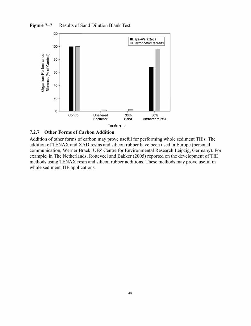
48

Figure 7–7 Results of Sand Dilution Blank Test

7.2.7 Other Forms of Carbon Addition Addition of other forms of carbon may prove useful for performing whole sediment TIEs. The addition of TENAX and XAD resins and silicon rubber have been used in Europe (personal communication, Werner Brack, UFZ Centre for Environmental Research Leipzig, Germany). For example, in The Netherlands, Rotteveel and Bakker (2005) reported on the development of TIE methods using TENAX resin and silicon rubber additions. These methods may prove useful in whole sediment TIE applications.

49

8 Phase I Overview and Methods: Interstitial Water This section describes characterization (Phase I) procedures for interstitial water and other aqueous preparations from sediments. Following the guidance in Section 6, use of these procedures for sediment TIE presumes that the IW from the sediment is toxic, and that an appropriate test organism has been selected. Phase I procedures for IW are patterned closely after those used for other water column samples with some changes. When procedures do not deviate from those used for effluents and ambient waters, we do not describe them in detail. Therefore, in order to use this guidance, it is essential to be familiar with TIE manuals for effluents and ambient waters (USEPA 1989a; 1991a; 1991b; 1992b; 1993a; 1996) Perhaps the greatest practical challenge in conducting TIE testing on IW is the difficulty in obtaining sufficient amounts of IW. With this in mind, the set of Phase I manipulations recommended for Phase I has been reduced from those recommended for effluent or ambient water TIE. As in previous guidance, we recommend the TIE begin with initial testing to determine the toxicity of the sample, which, among other things, aids in determining the dilution series to be used in the full Phase I. The Phase I itself consists of six procedures (Figure 8–1):

• Baseline Test – to determine the toxicity of unaltered IW; serves as a point of comparison for other manipulations

• Aeration Test – to evaluate volatile, sublatable (solid deposition onto a surface via the surface of air bubbles), or easily oxidized toxicants

• Solid-Phase Extraction (SPE) Test – targeted to remove nonpolar organic toxicants • EDTA Addition Test – to address cationic metals • Ulva Addition Test (marine only), or Zeolite Test – to remove ammonia • Graduated pH – to evaluate the pH sensitivity of the toxicity

Figure 8–1 Overview, Phase I Interstitial Water Characterization Tests

50

Each of these manipulations has been divided into three sections: overview, method, and interpretation. Tests that have been eliminated from the original Phase I characterization for water column samples (USEPA 1991a; 1991b) are the oxidant reduction (thiosulfate addition) test, the filtration tests, and the pH adjustment tests, including filtration, aeration, and SPE at high and low pH. The oxidant reduction test was eliminated from Phase I because the conditions in natural sediments are such that oxidizing compounds potentially found in effluents (e.g., chlorine) are not likely to occur in sediments. Thiosulfate addition does affect the toxicity of some metals and can be useful in identifying specific metals (Hockett and Mount 1996; Schubauer-Berigan et al. 1993). However, given that EDTA is a fairly robust test for metals, we are recommending using thiosulfate addition as a Phase II procedure, rather than a routine part of Phase I. Filtration through 1 μm glass fiber filters has been found to reduce the toxicity of many IW samples, but we are suggesting that it be dropped from Phase I as well because we believe that this removal is rather nonspecific, or at least it occurs by several mechanisms. Therefore it would not add a lot of diagnostic power to the Phase I, even if it does reduce toxicity. However, filtration has another important use in Phase I: its use as a pretreatment for the SPE manipulation, removing particulates so that the SPE column doesn’t clog. For IW TIE, we suggest that double centrifugation be used to remove particulates, and that the SPE test be conducted without prefiltration. Section 8.3.5 contains a more detailed discussion of this change and its implications. The pros and cons of performing the aeration, filtration, and SPE manipulations at high and low pH in Phase I have been debated since the issuance of the original TIE guidance in the late 1980s. On the positive side, pH sensitivity of these manipulations has been shown for many toxicants, such as precipitation/filtration of cationic metals at high pH, increased volatility of sulfide and cyanide at lower pH, and degradation of certain chemicals at extreme pH (e.g., malathion degradation at pH 3). All of these behaviors provide significant information to aid in either the identification or confirmation of the suspect toxicants. However, inclusion of these manipulations greatly increases the time required to perform the Phase I manipulations and, perhaps more importantly for IW TIE, the volume of sample required to complete Phase I. Based on our current experience, we believe reducing the volume of IW required is a significant benefit of eliminating these extra manipulations, and are therefore recommending that the manipulations at extreme pH be reserved as manipulations to be conducted during Phase II as required. These and the other deletions are being done primarily for expediency, and there is no reason they couldn’t be included in Phase I if the investigator feels they would be helpful. In general, we are making the presumption that IW TIEs will have lethality (LC50) as the endpoint. While this is not a technical requirement, all the IW TIEs we have performed to date have used lethality as the endpoint; all sublethal endpoints for which we have conducted sediment TIEs have been performed using whole sediment tests in freshwaters.

8.1 Interstitial Water Toxicity Test Procedures Because the procedural requirements for IW toxicity testing vary according to the species chosen for the TIE, specific definition of procedures that must be followed is not possible. Nonetheless, there are procedures we have found to work for many species, and several issues that should be considered before deviating from those methods.

51

8.1.1 Test Chambers Because of the difficulty in obtaining large volumes of IW, our IW TIE work to date has focused largely on species that can be tested in very small chambers in very small amounts of water. Our standard approach is to use 30-mL beakers containing 10 mL of test solution. This combination has been used successfully with Ceriodaphnia dubia, Daphnia pulex, Daphnia magna, Lumbriculus variegatus, Pimphlales promelas (fathead minnow larva), Americamysis bahia mysid shrimp, and Ampelisca abdita at a density of five organisms per beaker. Other investigators have successfully performed TIEs using 10 mL of water in 20 mL scintillation vials with one E. estuarius/replicate or five H. azteca/replicate (Anderson et al. 2006a). Some organisms, such as Hyalella azteca and midge larva (Chironomus sp.) do not adapt well to water column exposure unless some form of substrate is included. We have used a very thin layer of clean quartz sand on the bottom of the beaker as a comparatively inert substrate for this purpose. For H. azteca, many researchers have used small pieces of nylon screen or webbing as a substrate during water column testing; however, there is evidence that this nylon material may serve as a significant sorbent for organic compounds and so we recommend the quartz sand instead, which seems to provide the required substrate with less tendency toward chemical sorption (unpublished data, C. Ingersoll, USGS, Columbia, MO, USA). Previous TIE guidance has also suggested the use of plastic beakers for TIE testing (USEPA 1991b; 1992b). Plastic beakers have the advantage of being both inexpensive and disposable. While these were proven effective for most TIEs on effluents, sediments have a greater tendency to contain chemicals with high KOW which may sorb excessively to plastic chambers. For this reason, we generally recommend that IW TIEs be conducted in glass beakers rather than plastic. If the investigator has a strong desire to use plastic beakers (i.e., metal contamination is suspected), the initial and baseline toxicity tests should contain at least one replicate conducted in glass beakers, so the effect of plastic versus glass can be determined.

8.1.2 Test Design IW tests are generally run in dilution series, using a 0.5 x dilution ratio. Thus, an initial IW toxicity test might be run at 100, 50, 25, 12.5, and 6.25 % IW plus a dilution water control. For the Phase I tests, there is no specific number of dilutions that must be tested, and the dilution series may vary depending on the degree of toxicity in the sample. A typical dilution series for Phase I might be 100, 50, 25, and 12.5 % IW, plus the procedural blank. To prevent extreme levels of toxicity from “overpowering” the Phase I manipulations, the intention is generally to have the top concentration be no higher than 4 x the LC50. Where the IW LC50 is less than 25%, the highest concentration in the test would be diluted to achieve approximately 4 x the IW LC50, then a 0.5 dilution series would be prepared from there (e.g., 4 x, 2 x, 1 x, and 0.5 x).

Note: In this case it may be advisable to dilute the IW down to the highest test concentration before performing the manipulations. In cases where the LC50 is greater than 50%, a dilution series that includes 100, 75, 50 and 25% may be used.

8.1.3 Volume Considerations The actual sample volume needed to conduct the TIE tests depends on the 24-hour LC50 from the initial interstitial water test (Table 8–1). All volumes listed assume the initial LC50 is greater than 25%. If the initial LC50 is less than 25%, a smaller sample volume would be needed because of the necessity to dilute to 4 x the LC50 for subsequent testing and TIE work. If there are logistical

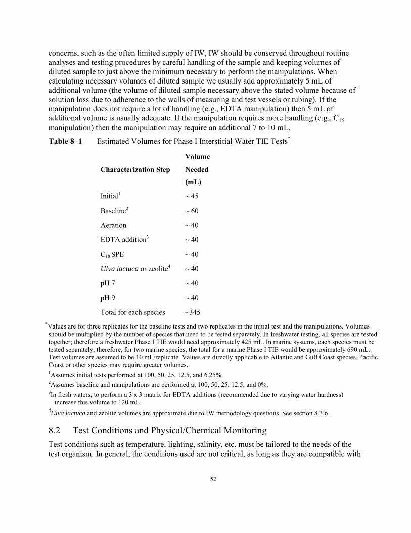
52

concerns, such as the often limited supply of IW, IW should be conserved throughout routine analyses and testing procedures by careful handling of the sample and keeping volumes of diluted sample to just above the minimum necessary to perform the manipulations. When calculating necessary volumes of diluted sample we usually add approximately 5 mL of additional volume (the volume of diluted sample necessary above the stated volume because of solution loss due to adherence to the walls of measuring and test vessels or tubing). If the manipulation does not require a lot of handling (e.g., EDTA manipulation) then 5 mL of additional volume is usually adequate. If the manipulation requires more handling (e.g., C18 manipulation) then the manipulation may require an additional 7 to 10 mL.

Table 8–1 Estimated Volumes for Phase I Interstitial Water TIE Tests*

Characterization Step

Volume

Needed

(mL)

Initial1 ~ 45

Baseline2 ~ 60

Aeration ~ 40

EDTA addition3 ~ 40

C18 SPE ~ 40

Ulva lactuca or zeolite4 ~ 40

pH 7 ~ 40

pH 9 ~ 40

Total for each species ~345 *Values are for three replicates for the baseline tests and two replicates in the initial test and the manipulations. Volumes should be multiplied by the number of species that need to be tested separately. In freshwater testing, all species are tested together; therefore a freshwater Phase I TIE would need approximately 425 mL. In marine systems, each species must be tested separately; therefore, for two marine species, the total for a marine Phase I TIE would be approximately 690 mL. Test volumes are assumed to be 10 mL/replicate. Values are directly applicable to Atlantic and Gulf Coast species. Pacific Coast or other species may require greater volumes. 1Assumes initial tests performed at 100, 50, 25, 12.5, and 6.25%. 2Assumes baseline and manipulations are performed at 100, 50, 25, 12.5, and 0%. 3In fresh waters, to perform a 3 x 3 matrix for EDTA additions (recommended due to varying water hardness)

increase this volume to 120 mL. 4Ulva lactuca and zeolite volumes are approximate due to IW methodology questions. See section 8.3.6.

8.2 Test Conditions and Physical/Chemical Monitoring Test conditions such as temperature, lighting, salinity, etc. must be tailored to the needs of the test organism. In general, the conditions used are not critical, as long as they are compatible with

53

the test organism, are kept the same for all tests, and don’t conflict with the overall goals of the TIE (i.e., conflict with those in the original toxicity test). Important chemical/physical endpoints to be monitored include temperature, dissolved oxygen (DO), pH, salinity/conductivity, ammonia, hardness, and alkalinity. For some manipulations, such as the pH manipulation, monitoring should be performed more often than during a standard toxicity test.

8.2.1 Temperature Temperature should be monitored daily, with sufficient sampling across treatments, tests, and the spatial area in which the tests are conducted to ensure that temperature does not vary substantially across the system. The mean temperature is less important than the consistency of temperature across test chambers.

8.2.2 Dissolved Oxygen DO should be measured in a subset of test chambers every day. Monitoring for DO is primarily to ensure that any toxicity observed is not the result of insufficient oxygen and, therefore, the intensity of DO monitoring should be designed to provide this assurance. Because 100% IW is typically the treatment with the highest oxygen demand, DO monitoring should be conducted with a heavy emphasis on these treatments. In addition, DO should be measured in any treatments showing marked biological effects, to ensure these effects are not related to DO.

8.2.3 pH pH affects the toxicity of many chemicals, which makes it one of the more important measurements to make during TIE testing. In addition to ensuring that pH is within the physiological tolerances of the organisms, the purpose of pH monitoring is to determine whether differences in toxicity among treatments, or among dilutions within a test, are related to differences in pH. Accordingly, we recommend that pH is measured in the treatments with the highest IW concentration, in dilution water controls, and in test concentrations bracketing the threshold for any toxicity being observed. Beyond these general recommendations, the graduated pH test should be closely monitored for pH. However, the ability to measure pH may be affected by the test methodology chosen for this test; recommendations are included in the description of these tests (see Section 8.3.5).

8.2.4 Salinity For marine tests, salinity should be measured, and if necessary, adjusted daily. The small test volume and the need to allow for diffusion of air into the test sample all tend to increase evaporation, and therefore increase salinity. In order to maintain salinity within 1 to 2 ppt of the original salinity, it is often necessary to add a small aliquot of distilled water daily.

8.2.5 Conductivity, Hardness, Alkalinity Measurement of these parameters is restricted primarily to the initial characterization of the sample being tested; in general, additional monitoring is not conducted during actual toxicity testing. Conductivity should be measured in freshwater samples as a check that the dissolved ion concentrations are not inordinately high (e.g., 2000 μS/cm). Hardness and alkalinity are useful additional parameters for characterizing freshwater IW samples but again, need to be

54

measuredonly on the IW sample itself. Hardness is often quite high in freshwater IW samples, which may affect metal and ammonia toxicity.

8.2.6 Dilutions, Dilution Water Dilution of aqueous test samples is essential in order to track changes in toxicity by allowing the investigator to perform LC50 calculations for different manipulations. A clean, consistent source of dilution water is necessary to perform TIEs. For marine samples the dilution water should be the desired salinity of the test. Ho et al. (1995) concluded that there was no difference in TIE results whether the sample salinity was changed before or after the manipulations. For consistency, we recommended that all salinity adjustments be performed once at the beginning of the TIE. For freshwater samples, the dilution water is often matched into categories of hardness and alkalinity. While an exact match is not always necessary (or easily achieved), the dilution water should not be so different that the toxicity of metals or other toxicants would change dramatically.

8.2.7 Replication In the past, EPA has released guidance in the TIE effluent manuals recommending that TIE manipulations be performed without replication. This recommendation evolved in part from the logistic constraints imposed by the large number of manipulations performed under the effluent TIE methodology. Because of the reduced number of Phase I manipulations recommended for Phase I IW TIE, there may be opportunity to increase replication. If at all possible, we advise testing two replicates, or even three, particularly for the baseline test against which other tests are compared. Replication is particularly important when the magnitude of toxicity is low (e.g., only partial mortality in 100% IW). There is, of course, a tradeoff between increased replication (and the associated interpretive power) and the logistical ease of conducting a TIE.

8.2.8 Observations Careful and well annotated observations in IW TIEs may provide important information for toxicant identification and interpretation of test results. Observations can include, but are not limited to, formation of precipitate, time to death of organisms, unusual organism behavior, color or turbidity of IW, oily sheen, or any other aspects of IW appearance.

8.2.9 Feeding Some test organisms, such as the marine mysid A. bahia, require feeding for survival. For organisms that don’t need to be fed, but nevertheless may benefit or perform better when fed, we recommend feeding because it may reduce test variability in the long run. The major concern with feeding is that it may reduce the bioavailability of toxicants. While the possibility cannot be discounted, most interstitial waters contain comparatively high concentrations of dissolved organic carbon, which would be expected to reduce the effect of exogenous food on chemical bioavailability. A modified feeding regimen may also be used; in the case of the amphipod, A. abdita, if the test is performed for more than 96 hours we feed algae at 96 hours, then renew the IW after allowing 4 hours for organisms to feed.

8.2.10 Simultaneous Testing Another useful tool for reducing the volume and effort required for TIE testing with interstitial water is the simultaneous testing of two species in the same test chamber. This method provides the additional advantage of minimizing differences in chemical test parameters, for example, pH,

55

during the testing of two species, and allows for easy comparison of species sensitivity. We have successfully tested C. dubia and fathead minnow in the same 10 mL volume throughout an entire Phase I evaluation. However, when A. bahia and A. abdita were tested in the same 10 mL volume, we noted increases in EC50s probably due to sorption of toxicants to the organism biomass (Ho et al. 2000). While simultaneous testing has its advantages, we do not recommend simultaneous testing of species until it has been determined that the species are compatible, and that test conditions (e.g., adequate DO) can be maintained throughout the test.

8.3 Initial Tests The purpose of the initial tests is to determine if the IW is toxic and, if so, how toxic (i.e., to generate an LC50), in order to identify appropriate concentrations for the TIE manipulations. For the initial test, we recommend running at least duplicates and generally to test as many water column and benthic species as are currently collectable or available in our cultures. For each freshwater species (up to four), 45 mL of IW and 60 or more organisms of the same age are required. For marine species (we generally test two) we use 90 mL of water because our species must be tested separately and 60 organisms of the same age are required. A concentration series using 10 mL of 100, 50, 25, 12.5, and 6.25% IW should be prepared. If there is evidence that the toxicity of the sample is relatively low (i.e., EC50 = 75% IW), the dilution series may be adjusted upward to compensate and more IW (30 mL/species /replicate) may be needed. The concentration series also should have duplicate control cups (as a minimum) for each species tested. If after 24 hours the LC50 of the IW is at or below 6.25%, the test should be repeated using a lower dilution series (e.g., add 3.13% and 1.56%).

8.3.1 Baseline Test Overview If the initial toxicity test on the IW shows that it is acutely toxic (i.e., >50% mortality at a 100% sample dilution), Phase I TIE manipulations can be initiated. Samples with less than 50% mortality in 100% interstitial water can still be evaluated using IW TIE methods, but it can be more difficult to discern actual changes in toxicity relative to innate variability. Increased replication is very important when conducting TIEs on samples with minimal toxicity. Because the baseline test is used as the reference point to determine whether a manipulation has affected the toxicity of the sample, a baseline test should be included as part of every set of Phase I tests, even if tests are conducted on successive days. Temporal changes in the toxicity of IW are not uncommon, so a simultaneous comparison is critical.

Method The test concentrations of the baseline test are determined by the initial toxicity test. Exposure concentrations should be at 4 x, 2 x, 1 x, and 0.5 x the 24-hour LC50 of the initial test if the LC50 was less than 25% whole sample concentration. If the LC50 was greater than 25%, exposure concentrations are typically 100, 50, 25, and 12.5%. More condensed dilution series (e.g., 100, 75, 50, and 35%) can be used with samples having very low levels of toxicity. Because the baseline test serves as the point of comparison for all other tests, replication is strongly recommended (minimum duplicate, triplicate preferred).

56

Interpretation The baseline test provides the index response against which other tests are compared. Toxicity may be assessed in terms of overall LC50 or by the amount of mortality in specific dilutions. Another function of baseline tests is to track the stability of sample toxicity over time throughout the TIE. Changes in the baseline toxicity over time may indicate that volatile or unstable toxicants are present.

8.3.2 Volatile Compounds: Aeration Overview Aeration tests are designed to determine whether toxicity is attributable to volatile, oxidizable, or sublatable compounds. Samples are sparged with air for one hour, and tested for toxicity. If toxicity is reduced by air sparging, the presence of volatile or oxidizable compounds is suggested. To distinguish the volatile from the oxidizable compounds, further experiments are performed using nitrogen to sparge the samples rather than air. If toxicity remains the same as in the baseline toxicity test, oxidizable materials are implicated; if toxicity is again reduced, volatile compounds are suspected. An additional mechanism through which toxicants can be removed from a sample by aeration is sublation, which is movement of the compound through the aqueous phase on the surface of the air bubbles, followed by deposition as a solid on the aeration glassware at the air–water interface. If sublation were the mechanism through which sample toxicants were removed, it might be possible to recover this toxicity by rinsing the aeration glassware (Ankley et al. 1990b). Compounds possessing both polar and nonpolar characteristics, such as surfactants or resin acids, are particularly prone to sublation from aqueous samples.

Method The aeration tests and procedures remain identical to those described for effluent TIEs (USEPA 1991a; 1991b; 1996). Briefly, 40 mL of IW sample and a corresponding blank for each test species are placed into separate 100 mL graduated cylinders and aerated for one hour. The rate of aeration should be maintained at 500 mL/min. After one hour of aeration, the sample should be removed from the aeration vessel and transferred to a clean beaker using a siphon or pipette to prevent any re-solution of sublated compounds into the sample.

Interpretation A change in toxicity after aeration indicates the presence of a volatile, oxidizable, or sublatable toxin. A notable volatile toxicant in IWs is hydrogen sulfide. If hydrogen sulfide toxicity is suspected, another manipulation to confirm the presence of hydrogen sulfide toxicity is the graduated pH manipulation (Section 8.3.5). While forms of ammonia are gaseous and may be considered volatile, ammonia concentrations appear to be stable in seawater during aeration for up to 96 hours at pH 8. In order to remove ammonia by aeration, the pH must be increased to 10 (Burgess et al. 2003). Although this method is designed to remove volatile compounds, there may be circumstances when the toxicity may change due to the compounds’ oxidation state and not volatility. To distinguish volatile from oxidizable compounds, further experiments are performed using nitrogen to sparge the samples rather than air. If toxicity remains the same as in the baseline

57

toxicity test, oxidizable materials are implicated; if toxicity is again reduced, volatile compounds are suspected.

8.3.3 Organic Compounds: Reverse-phase Solid-phase Chromatography Overview Reverse-phase solid-phase chromatography is designed to determine the extent of sample toxicity due to compounds that are relatively nonpolar. This test, in conjunction with associated Phase II analytical procedures, is an extremely powerful TIE tool. In this procedure, sample aliquots are passed through small columns packed with an octadecyl (C18) sorbent. We have had the most experience with the C18 column, but other researchers have successfully used alternative packings such as Tenax (Cornelissen et al. 2001), C8 (Bailey et al. 1996), and other columns with lower binding affinity such as the hydrophilic-lipophilic balance sorbent (Oasis®); (Anderson et al. 2006a) in order to isolate organic toxicants. The C18 solid phase extraction (SPE) column removes neutral nonpolar compounds including PAHs, PCBs and some pesticides. The C18 column may also sorb particle-active metals such as copper or lead; therefore, this manipulation, like all of the recommended manipulations, should be used in a suite of manipulations and not as a stand-alone procedure. The C18 blank may include some hydrocarbons eluted from the plastic housing (Junk 1988) and, therefore, manipulation blanks should be performed for this (and all other) manipulations. The methods for the C18 SPE test are conceptually similar to those used for effluent TIE work (USEPA 1991b; 1992b; 1996) but there are differences in sample preparation, volumes, and the elution solvents. Because particulates in samples can plug the C18 column, samples must be pretreated to remove particulates before the SPE procedure. In effluent TIE, this is accomplished by prefiltering samples through glass fiber filter. In IW testing, we have observed a lot of seemingly nonspecific removal of toxicity by glass fiber filtration, and for this reason we recommend double centrifugation as an alternative. This involves an initial centrifugation of the sediment and decanting the IW, followed by a second centrifugation of only the IW to further remove residual particulates. The speed of these centrifugations depends on the equipment available in the laboratory. In general, centrifugation at 10,000 x g or more for at least 30 minutes is required in at least one of the steps to effectively remove fine particulates. After both centrifugations, great care should be given to preventing the transfer of particulates. Particularly after the second centrifugation, removal of IW by siphon or pipette is recommended (rather than simple decanting) to minimize the transfer of solids. Another difference from effluent TIE procedures is the use of different solvents for elution. Because sediments commonly contain chemicals with high KOW (e.g., >105) , methanol may not be sufficiently nonpolar to elute contaminants from the C18 column. For this reason, the elution solvents are modified to include less polar solvents, such as methylene chloride. Details are described in Section 9.3.2. A decision point when planning Phase I SPE testing is the timing of testing the eluate fractions: whether to proceed immediately, or to perform an additional extraction and elution as part of Phase II studies if Phase I is to be limited to determining whether SPE reduced toxicity of the IW. The advantage of including elution as part of Phase I is that it requires only a single SPE extraction, and does not require the isolation of additional IW or the preparation of a new SPE column. The disadvantage of conducting solvent elution of the column as part of Phase I is that if the postcolumn effluent does not change in toxicity, then no useful information is gained from

58

the effort used to collect and test the eluates. This of course assumes that the column has not been overwhelmed by the amount of organic contaminants that has passed through and breakthrough has occurred (USEPA 1992a). In addition, there is some evidence to suggest that IWs high in dissolved organic material may allow hydrophobic compounds to pass through the column. This has been noted in IWs from field sediments contaminated with pyrethriod pesticides (personal communication, B. Phillips, Marine Pollution Laboratory, Monterey, CA, USA). A third, intermediate, option is to collect and test a smaller number of solvent eluates. Finally, one might store the loaded C18 columns until the results of the Phase 1 tests have been received, although it is difficult to determine if holding time would change the toxic constituents. The selection among these options is at the discretion of the investigator; if organic contaminants are thought to be likely, then proceeding with elution as part of Phase I may be advisable.

Method The SPE test is generally conducted with a 3-mL (for up to 300 mL sample) or a 6-mL (for up to 1 L) C18 column, though larger columns (e.g., 12-mL) have been used. Whether or not the column is eluted as part of Phase I, the column must be first conditioned with methanol and water (USEPA 1991b). Next, the extraction blank is prepared by pumping dilution water over the column in a volume equal to the volume of IW to be extracted. The next step depends on which procedure option is pursued in Phase I. If the approach is to test the postcolumn IW for toxicity (no solvent elution), then the next step is to pass the IW over the column, collect aliquots of the postcolumn sample, and test for toxicity. If a complete solvent elution is conducted, then the methodology is the same as that described in Section 9. Briefly, the column is conditioned, followed by the dilution water blank and the full series of elution blanks. The column is then re-conditioned, followed by the interstitial water sample, and the solvent fraction series. Aliquots of the post-column interstitial water and the eluted fractions are tested as described in Section 9.3.2. If the abbreviated elution is conducted, the procedure is similar to the full elution method, but with fewer solvent fractions. The column is first conditioned with methanol and water; then the dilution water blank is passed through the column. Next, extraction blanks are collected by passing three aliquots of 100% methanol, followed by three aliquots of methylene chloride. These six fractions (three from each solvent) can be combined, volume reduced (or exchanged) and tested as a single fraction. In addition to being more nonpolar than methanol, methylene chloride is miscible with methanol and has the additional quality of being more volatile than methanol. These two properties allow a solvent transfer of the methylene chloride fractions and blanks into methanol before toxicity testing. This step is essential because methylene chloride is more toxic to aquatic organisms than is methanol (e.g., the former has a 48-hour C. dubia LC50 of 0.46%, while that for methanol is 2.1%). The transfer is accomplished by partially evaporating the fractions and blanks containing methylene chloride with nitrogen (until the methylene chloride is removed) and subsequently restoring the initial volume with methanol (see Section 9.3.2 for more details on exchanging solvents). The blank fractions are treated similarly. The 100% methanol fractions and their corresponding blanks then are tested as described elsewhere (USEPA 1991b; 1992b). Most freshwater organisms with which we have worked can tolerate 1.2 % methanol in water (e.g., 240 μL of methanol extract in 20 mL of dilution water). The methanol tolerance for several test organisms are given in Table 8–2 and in the effluent TIE guidance (USEPA 1991b; 1992b). A. abdita is particularly sensitive to methanol (A. abdita 96-

59

hour LC50 is 0.75%) and requires a lower methanol addition than the suggested 1.2%. In general, we recommend that methanol addition not exceed 25 to 50% of the LC50 for that species.

Table 8–2 Species Sensitivity to Phase I Additives LC50 (g/L unless otherwise noted)

Additive Species SW1 MHW2b HW3 30 ppt

EDTA H. azteca 0.08 0.16 0.23 L. variegatus 7.0 7.4 M. lateralis4 0.288 A. abdita 0.150 M. bahia 0.315

Methanol H. azteca 2.6% L. variegatus 6.1% M. lateralis4 2.2% A. abdita 0.75% M. bahia 2.3%

NaCl H. azteca 3.9% L. variegatus 7.0 7.4%

1SW, soft water, natural or reconstituted 3HW, hard water, reconstituted 2MHW, moderately hard water, reconstituted 4Salinity, EC50 values for M. lateralis are for 48 hours; all other data are based on 96 hours

The concentration of toxicants in the fraction tests (relative to 100% IW) differs based on the volume of IW extracted, the volume of the extract, and the dilution of methanol used in the fraction test. The concentration factor is calculated based on the aggregate of the concentration or dilution factors at each step and assumes 100% recovery of toxicants. For example, if 300 mL of IW is reduced to 1 mL of methanol, the methanol fraction is at 300 x the IW. If this fraction is then tested by adding 240 μl of methanol to 20 mL of dilution water, the resulting dilution is dilution factor is 83.3-fold, and the final concentration in the fraction test is 300/83.3 = 3.6 x the concentration in the original IW. In order to account for possible procedural losses, the investigator should target the concentration in a eluation fraction test to be equivalent to at least twice the LC50 in the IW, and preferably higher. To achieve that concentration, it may be necessary to concentrate the methanol fractions additionally, particularly for methanol-sensitive species such as A. abdita.

Interpretation Decreased toxicity in the post-C18 effluent and capture of the toxicity in the column eluate is a powerful indicator of organic toxicity. Further fractionation and identification of individual or groups of compounds can give insight into sources and stressors active in sediments. In our experience, organic compounds are a common source of toxicity in sediments, presumably because sediments are a common sink for persistent, hydrophobic compounds in the aquatic environment. However, the C18 column can also act as a filter, or as a nonspecific binding medium for cationic metals (e.g., copper, lead). For this reason, removal of toxicity by SPE alone

60

does not necessarily indicate toxicity from organic compounds; accompanying recovery of toxicity in the SPE fractions is an important confirmation. This need for recovery of toxicity is a major reason we suggest that investigators consider including column elution as part of the Phase I SPE test. On the other hand, while recovery of toxicity from the C18 column eluate is a strong indicator of organic toxicity, lack of toxicity in the eluate does not necessarily indicate that organics are not responsible. Many hydrophobic compounds may not be recoverable from C18 or other columns (Anderson et al. 2006a). It is important to consider the results of the SPE test in conjunction with other Phase I manipulations (e.g., EDTA) to provide context for interpreting SPE findings.

8.3.4 Cationic Metals: EDTA Test Overview The presence of toxicity due to cationic metals is tested through additions of ethylenediaminetetraacetic acid (EDTA), a strong chelating agent that produces nontoxic complexes with many metals. The specificity of the EDTA test for a class of ubiquitous toxicants makes it a powerful TIE tool. Cations chelated by EDTA include certain forms of aluminum, barium, cadmium, cobalt, copper, iron, lead, manganese, nickel, strontium, and zinc (Stumm and Morgan 1981). EDTA does not complex anionic forms of metals, and only weakly chelates certain cationic metals, for example, silver, chromium, and thallium (Stumm and Morgan 1981). EDTA appears to preferentially bind these transition metals over calcium and magnesium (hardness ions), and in-house studies suggest that the equilibration time for heavy metal chelation by EDTA is relatively brief. Despite the concern over water salinity, EDTA additions are effective in removing toxic cations in aqueous marine samples (Stumm and Morgan 1981; USEPA 1996). In addition, cation exchange resins have been demonstrated to be useful in removing toxic cations (see Phase II, Section 9; Burgess et al. 2000; Burgess et al. 1997; USEPA 1996). A range of IW concentrations is used in conjunction with varying additions of EDTA to help determine the degree of toxicity associated with cationic metals in the IW sample. Because water hardness may affect the toxicity of EDTA as well as its ability to chelate toxic cationic metals, sample hardness should be considered when test concentrations of EDTA are set. To aid in identification of appropriate test concentrations for freshwater species, the toxicity of EDTA to the TIE test species must be ascertained for water with a hardness typical of that in the IW. Table 8–2 indicates these values for H. azteca and L. variegatus; data are also given for the marine species A. abdita and A. bahia at 30 ppt salinity. Comparable data for selection of appropriate EDTA concentrations for C. dubia and fathead minnow and other marine species are described elsewhere (USEPA 1991b; 1996; 2002a).

Method For fresh water, we generally use and recommend the dilution option described in the effluent TIE document (USEPA 1991b). This consists of testing three dilution series of 100, 50, and 25% IW (or 4 x, 2 x, and 1 x the LC50 for highly toxic samples). To each of these dilution sets is added one of three decreasing concentrations of EDTA, thus forming a 3 x 3 matrix of EDTA level versus IW concentration. The three quantities of EDTA added should range from an amount approximating the LC50 of EDTA for the organism to a quantity that should not be toxic. Typical EDTA concentrations used are the EDTA LC50, 0.5 x EDTA LC50, and 0.25 x EDTA

61

LC50, using an EDTA LC50 value appropriate for the sample hardness, which is often high in IW. In marine IW TIEs , we have generally tested at a single concentration of EDTA, 30 mg/L (USEPA 1996), which is tolerated by all marine organisms we have worked with. There is some evidence that this concentration of EDTA may decrease the test pH, and be too high for M. galloprovincialis (personal communication, D. Greenstein, Southern California Coastal Water Research Project, Costa Mesa, CA). Mortality in manipulation blanks would be a signal that EDTA concentrations are too high for the test organism. We recommend tolerance testing of species other than those listed in Table 8–2 in order to ensure that EDTA concentrations are not toxic. For both marine and freshwater EDTA testing, a three-hour interaction period is allowed after EDTA addition and before the animals are added to the IW. Blank tests of dilution water with EDTA added are included to ensure that the EDTA additions alone are not toxic.

Interpretation Reductions in sample toxicity from EDTA addition are generally reasonably specific for toxicity caused by cationic metals. On occasion, high concentrations of EDTA may reduce pH of the sample, which can alter the toxicity of certain toxicants (e.g., ammonia, sulfide). Monitoring of pH and/or adjustment as necessary is recommended as a safeguard against such interferences.

8.3.5 Graduated pH Manipulation Overview Adjusting the interstial water pH can be a very powerful tool in sediment TIE. The bioavailability and toxicity of ammonia, hydrogen sulfide, and metals are highly pH dependent, even within the relatively narrow range of physiological tolerance for most pelagic, epibenthic, and benthic organisms (pH 6 to pH 9 for freshwater organisms and pH 7 to pH 9 for marine organisms). Because the graduated pH test is the only manipulation that targets toxicants with pH dependence, the results are often the first and only substantive clue to pH-dependent toxicants in the sample. For IW TIEs, the power of pH adjustment as an investigative tool must be balanced against the practical constraints on obtaining large quantities of IW for testing. In the TIE guidance for effluents and ambient waters, pH manipulation is used in two ways:

• A graduated pH test in which the sample is tested for toxicity at multiple pHs • “pH adjustment” tests in which pH of the sample is adjusted to acidic or basic conditions,

then returned to the original pH and tested for toxicity. These pH adjustment procedures are also used in concert with filtration, aeration, and solid-phase extraction to evaluate changes in toxicant behavior at extreme pHs.

Because of the limited sample volumes in IW TIE, we recommend that Phase I investigations begin with only the graduated pH test. The other pH adjustment tests can be performed in a tiered investigation if insufficient evidence is obtained during the initial Phase I without pH adjustment tests (see Section 9.7). Ammonia is perhaps the most widely encountered toxicant that is pH sensitive and responds characteristically in the graduated pH test. Because ammonia is a common constituent of IW and because it is relatively easily measured (see Section 6), IW ammonia measurements should be taken at the beginning of each test. Figure 8–2 shows the change in relative ammonia and ammonium concentrations with change in pH. The exact roles of ammonia and ammonium in

62

aquatic toxicity have been debated, but it is accepted that un-ionized ammonia is the more toxic of the two forms for most species (Erickson 1985; Miller et al. 1990; Russo 1985). Therefore, the combined toxicity of a given total ammonia concentration generally increases with increasing pH, because of the relatively higher proportion of total ammonia present as un-ionized ammonia as pH increases. While pH is a dominant factor in determining the toxicity of ammonia to most aquatic species, ammonia toxicity to H. azteca appears more complex and has been found to depend on several factors (see Section 9.1; Ankley et al. 1995; Borgmann and Borgmann 1997).

Figure 8–2 Change in Relative Ammonia Concentrations with Change in pH for Selected Temperatures*

*Data calculated using the dissociation constants for ammonia (USEPA 1979). Under constant temperatures, as pH increases by one unit, there is 10-fold increase in the percent of un-ionized ammonia NH3 present in aqueous solutions at pH 6.0 to 9.0. USEPA’s ammonia water quality criteria document is an excellent source for the discussion of ammonia (USEPA 1985a).

The graduated pH test is another line of evidence for (or against) ammonia toxicity. With a dissociation constant (pka) slightly above pH 9, the speciation of ammonia changes dramatically relative to the range of pH 6 to 9 common to natural waters. The relative concentration of un-ionized ammonia increases as pH increases within this range. For example, in freshwater at 25°C the concentration of un-ionized ammonia (relative to ionized ammonia) is only about 0.05% at pH 6, but increases to about 5% at pH 8. In addition to the speciation change, it appears that the toxicity of the forms of ammonia may also change with pH (Miller et al. 1990; USEPA 1985a). However, the net result for most aquatic species is that the same total ammonia concentration is about three times more toxic at pH 8 than at pH 6 (Table 8-3). If ammonia is the sole sample toxicant, an IW that is toxic at pH 8 or 9 may be nontoxic at the lower pHs tested in the graduated pH test. The toxicity of hydrogen sulfide is also highly pH dependent; the same concentration of total sulfide is approximately twelve times more toxic at pH 6.5 than at pH 8.7, even though molecular hydrogen sulfide appears more toxic at pH 8.7 than at lower pH (Broderius and Smith

63

1977). Often, in the graduated pH test, we have observed increased toxicity of IW at pH 6.5, which tends to disappear after storage of the interstitial water for more than 1 day. This behavior is consistent with hydrogen sulfide because of its high volatility and susceptibility to oxidation, which make it relatively unstable in isolated IW exposed to air.

Table 8–3 Relative Sensitivity (EC50) of Benthic and Water Column Test Species to Different Toxicants

Species

Ammonia

mg/L (95% CI)

CuSO4 μg/L

(95% CI)

SDS mg/L

(95% CI)

H2S

(mg/L)1

Black Rock Harbor Sediment

% sediment2 (95% CI)

Ampelisca abdita 0.833 (0.76–0.92) 14

(8–22)

Eohaustorius estuarius 2.493 (2.26–3.38) 3.32 21

(16–28)

Rhepoxynius abronius 1.593 (1.46–1.72) 1.6

Grandidierella japonica 3.353 (3.05–4.46)

Leptocheirus plumulosus 11 (8–33)

Hyallela azteca 0.834 (0.62-1.22)

365 (21-61)

Champia parvula 1.46 (0.8–1.9)

0.36 (0.2–0.4)

Arbacia punctulata 33.26 (17.2–50.8)

3.26 (2.6–5.1)

Mysidopsis bahia 2.987 (2.75–3.25)

169.36 (137.4–196.4)

9.36 (5.9–14.5)

Strongylocentrotus purpuratus 0.19

Mytilus edulis (embryo) 0.1 1Knezovich et al. (1996) 4Ankley and Schubauer-Berigan (1995) 2Calculated from Schlekat et al. (1995) 5Borgmann et al. (2005) 3Kohn et al. (1994) 6Morrison et al. (1989)

7Miller et al. (1990)

Metals form another class of compounds whose toxicity and bioavailability depend on pH within the range of the graduated pH test. Work with both pelagic (C.dubia, fathead minnow) and epibenthic–benthic species (H. azteca, L. variegatus) indicates that zinc and nickel show increased toxicity at pH 8.5 relative to that at lower pHs (Table 8–4). Lead and copper show the opposite trend, and are more toxic at pH 6.5 than at pH 7.5 or pH 8.5. For fathead minnows,

64

Table 8–4 Trends in Metal and Ammonia Toxicity with Respect to Test pH* Freshwater pH 6–6.5 7–7.5 8–8.5 Marine pH 6.5–7.5 7.5–8.5 8.5–9.2 Metal Species LC50 LC50 LC50 LC50 Zn C. dubia >530 360 95 H. azteca 1,200 1,500 289 P. promelas 830 333 502 C. dubia >200 137 13 M. bahia 340 460 580 A. abdita 2,860 4,470 1,970 Ni H. azteca 1,960 1,940 890 P. promelas >4,000 3,360 3,080 C. dubia 280 >2,700 >2,700 M. bahia 310 610 720 A. abdita 7,660 >10,100 9,400 Pb H. azteca <90 >5,400 >5,400 Fathead minnow 1,410 >5,400 >5,400 C. dubia 10 28 201 M. bahia 17,860 6,090 >2,500 A. abdita 12,300 11,300 >6,800 Cu Fathead minnow 15 44 >200 H. azteca 17 —1 87 C. dubia 563 350 121 M. bahia 110 250 360 A. abdita 160 90 30 Cd Fathead minnow 54 74 <5 H. azteca 228 — 4–15 M. bahia — 120 90 60 A. abdita — 1,780 1,260 1,540 Total NH3 H. azteca 202 (9.0) 232 (14) 212 (12) Un-ionized NH3 L. variegatus >1,000 62 13 — M. bahia3 — 163 38 1.39 A. abdita — — — 1.49 *LC50s (expressed as μg/L of metal or mg/L of ammonia) were determined at 48 hours for C. dubia and 96 hours for P. promelas, H. azteca, L. variegates, A. bahia, and A. abdita. Freshwater tests were performed in very hard reconstituted water. 1—Test not performed 2Value represents the mean of six LC50 values determined at that pH, with the standard deviation in parentheses 3Miller et al. (1990) cadmium appears to be more toxic at pH 6.5 and pH 8.5 than at neutral pH. In marine waters, nickel and copper demonstrated increased toxicity at lower pHs for M. bahia. Lead and copper showed the opposite trend (increased toxicity with increased pH) for M. bahia and A. abdita, respectively. Interestingly, zinc and copper did not demonstrate pH-specific toxic responses for the two organisms tested (Ho et al. 1999b). Thus, the graduated pH test may serve additionally to

65

distinguish between toxic and nontoxic metals when several are present simultaneously in an IW sample. The exact pHs tested in the graduated pH test are not particularly critical; the most important issues are achieving a range of pHs so that changes in toxicity may be observed, and staying within the physiological tolerance range of the test organisms. In work with freshwater sediments, we have found that after isolation and oxygenation, the IW often tend toward a pH of roughly 8.5. Accordingly, pHs of 6.5, 7.5, and 8.5 are often used. Marine organisms are less tolerant of pH below 7, so pHs of 7, 8, and 9 have been used more typically for marine TIE. While the concept of the graduated pH test is simple, there are a great many variations on it. Several different methods have been developed, each with its own advantages and disadvantages. In the sections below, we describe three of the most common methods:

• Carbon dioxide method – The concentration of CO2 in the headspace above the interstitial water is altered, which in turn alters the solution pH.

• Zero-headspace method – Hydrochloric acid or sodium hydroxide are used to adjust the pH of the sample; then the chamber is sealed without headspace, which helps maintain the adjusted pH of the sample.

• Buffer method – Relatively nontoxic hydrogen ion buffers are added to the interstitial water to maintain different pH levels.

8.3.5.1 Carbon Dioxide Method Overview The pH of freshwater and marine waters is controlled in large part by equilibria within the carbonate system:

CO2 + H2O = H2CO3 = H+ + HCO-3 = 2H+ + CO3 =

As such, increasing the partial pressure of CO2 creates carbonic acid (H2CO3); carbonic acid dissociates into bicarbonate (HCO3

-) and a proton, and bicarbonate may further dissociate into carbonate (CO3

2-) and another proton. Thus, increasing CO2 yields protons and therefore reduces pH. The reverse is also true: decreasing carbon dioxide consumes protons and increases pH. This relationship is exploited by the CO2 method for the graduated pH test. Samples of IW are tested under conditions of higher or lower CO2 (relative to ambient air) to produce test solutions with differing pH. Method A variety of test systems can be used for the CO2 methods; the general requirement is that the test beakers be placed within a sealed chamber constructed of glass or another substance that is relatively impermeable to CO2. For purposes of discussion, we refer to the enclosure within which the CO2 concentration is manipulated as the “CO2 chamber,” as contrasted with the “test chamber,” which refers to the beaker containing the IW and test organisms. The CO2 concentration in the headspace of the CO2 chamber is altered by either flushing it with gas of a specific CO2 concentration, or a measured volume of 100% CO2 can be added to the ambient air to produce the desired CO2 concentration in the headspace. CO2 chambers may have headspaces that are either flow-through or static; flow-through systems require cylinders of premixed gas to provide continuous flow at a fixed CO2 concentration, but have the advantage of continuously maintaining the desired concentration of CO2 in the headspace. Static headspace chambers are

66

susceptible to changes in CO2 concentrations as a result of exchange with the test solutions and/or production of CO2 by biological respiration, though they have the advantage of greater simplicity. Another issue that requires consideration in selecting a test apparatus is the potential for volatilization of toxicants and subsequent transfer of toxicant to adjacent test beakers. As an example, ammonia becomes volatile when present in the un-ionized form, which predominates at higher pH. If tests are conducted such that all test concentrations of IW are housed in the same chamber, then the higher ammonia concentrations present in the IW concentrations may volatilize ammonia that may be taken up by lower concentrations such as the controls. This can be avoided by housing different IW concentrations separately, but this in turn increases the number of CO2 chambers required. The same considerations apply to hydrogen sulfide, except that volatilization is highest at low pH. If all IW concentrations are housed together, systems using flow-through gas mixtures may be advisable as they flush some of the volatilized toxicant out of the chamber headspace. Separation of test beakers by concentration may be more easily achieved using static headspaces, for which the management of multiple CO2 chambers is much easier. An important point of reference for the CO2 test is the pH toward which the IW tends when equilibrated with ambient air (about 0.04% CO2); this can be determined from the pH measured in the 100% IW concentration of the baseline toxicity test. The air-equilibrated pH of IW varies depending on its source and composition. Marine IWs tend to be more consistent in pH, typically about 7.8 to 8.2 after air equilibration (they are often slightly more acidic immediately after isolation but tend upward after air equilibration). IWs from freshwater sediments are more variable; while many equilibrate in the range of 8.3 to 8.5, some may be more acidic, particularly those with high concentrations of iron. Because marine IWs often tend toward pH 8 after equilibration, and marine organisms are not very tolerant of low (<7) pH, we have typically conducted graduated pH tests with marine organisms at target pHs of 7, 8 (ambient), and 9; pH 7 is typically achieved using 2% CO2, while pH 9 is achieved using CO2-free air. Freshwater organisms are generally more tolerant of pH in the range of pH 6 to 7, and we have often used target pHs of 6.5, 7.5, and 8.5 in the graduated pH test. However, the selection of specific pHs is somewhat arbitrary; all that is really needed is a reasonable range of pH so that changes in toxicity may be observed. Because the chemistry of IW from freshwater sediments can vary among sediments, some trial and error may be required to determine the CO2 concentrations necessary to achieve the desired pHs. For IWs that air-equilibrate in the range of pH 8.0 to 8.5, appropriately lower pHs can generally be achieved using 8 to 10% CO2 for the lowest pH (e.g., 6.5) and 2 to 5% for a middle pH (e.g., 7.5). Again, the exact pH is not that important, rather that a range of pH is achieved. Concentrations of CO2 much above 10% may cause toxicity to some test organisms. The pH of dilution water may respond differently to CO2 from that of IW, so controls and/or dilutions may end up with different pH at the same CO2 concentration. Premixed gases with defined CO2 content can be obtained from most specialty gas suppliers.

67

Safety Note: Elevated concentrations of CO2 are a potential health risk to people. While small volume releases of gases with low percentages of CO2 are generally diluted by large volumes of room air, even 10-minute exposures of a person to CO2 concentrations of 1 to 3% may be dangerous and must be avoided. All uses of CO2-enriched gases must be conducted with appropriate ventilation. Effluent air from chambers with continuous headspace renewal must be vented so as to avoid worker exposure.

Any number of different vessels may be used as the CO2 chambers. Large systems designed to contain entire tests may be constructed from sheet glass, but the lids must be affixed with some kind of gasket to limit leakage of the headspace gas. If the system is flow-through, plastic chambers may be used; for static headspace chambers, plastic is less desirable, as many plastics are CO2-permeable. Influent and effluent ports are required for introducing and venting the headspace, particularly for flow-through chambers. Alternatively, smaller chambers that hold only a small number of test chambers may be used. Wide-mouth, screw-top jars (e.g., canning jars) can be useful in this regard. Such chambers may be more effective for tests with static headspace (the headspace is flushed initially with gas, then sealed) and when different test concentrations of IW are separated from one another to prevent cross-contamination via volatilization. Another option is to combine the test chamber and CO2 chamber into a single vessel, such as by using 60-mL BOD (biological oxygen demand) bottles with ground-glass stoppers; test solution may be added directly to the bottle, and then the headspace flushed with gas and sealed. The CO2 method is generally performed with three separate dilution series of IW, one for each pH, with duplicate test chambers at each pH. For marine IWs, the relatively high buffering capacity generally requires that the pH of samples be adjusted with acid/base before being placed in the CO2 chambers. This is done by adding small amounts of 1 N HCl or 1 N NaOH to adjust pH to 7 and to 9, respectively. Typically about 25 μL is needed, but this depends on the amount of buffering material in the IW. This is best done in a stepwise fashion, being careful not to overshoot the target pH. If the target pH is passed and it is necessary to add either acid or base to return to the target pH, check the salinity of the sample to ensure that it has not increased significantly. Generally, it is necessary to add more acid or base for the higher IW concentrations to overcome the additional buffering capacity of organic matter. In general, this preliminary pH adjustment has not been necessary for freshwater IWs, but it could be used for samples with particularly high buffering capacity, where CO2 enrichment alone is insufficient to adjust pH. After pH adjustment with acid or base (if necessary), test chambers are placed into the CO2 chambers, the headspace is flushed with the appropriate gas mixture, and the system is allowed to equilibrate. The time for equilibration has not been carefully tested, and can be expected to vary with aspects of the chamber geometry, etc. In practice, for freshwater TIE we have typically allowed about two hours and then opened the chambers and checked pH of the test solutions; if sufficient adjustment of pH is not obtained, adjustment of the CO2 concentrations and/or acid/base addition may be necessary. For marine work we have generally allowed chambers to sit in the CO2 chambers overnight and then rechecked the pH and readjusted as necessary. For flow-through CO2 chambers, the rate of gas flow necessary to maintain pH depends on aspects of the chamber geometry and other factors. In our marine tests, we have used a CO2 chamber with roughly 12 L capacity and have found that a flow rate of 100 mL/min of 2% CO2 gas maintains a pH around 7. A flow rate of 150 to 300 mL/min of CO2-free air (sometimes

68

called “zero grade”) maintains a pH of about 9. Placing the highest concentrations of IW near the inlet to the CO2 chamber has sometimes resulted in better pH control across the test, but consideration should be given to the potential for contamination of other concentrations via volatilization. Following equilibration and any subsequent adjustments that are necessary, test organisms are added to all test chambers, the test chambers are returned to the CO2 chamber, and the headspace is flushed with the appropriate gas. For mysids, which require feeding during the test, we add a minimum number of Artemia necessary for the survival of the mysids (20 to 40 Artemia/mysid) every 24 hours. One of the most important aspects of all of the graduate pH methods is intensive monitoring of test pH. Measuring pH twice per day in at least one replicate test chamber of each concentration is desirable. If it is necessary to adjust the test conditions (i.e., CO2 concentration or flow or addition of HCl or NaOH) all replicate test chambers should be checked. It is important that relatively constant pH be maintained throughout the test in order to adequately test the effect of pH on sample toxicity. Some pH-sensitive toxicants, including ammonia and hydrogen sulfide, are relatively quick-acting toxicants, so unstable test conditions may lead to misleading or uninterpretable results.

Interpretation With respect to changes in toxicity as a result of pH manipulation itself, interpretation of the graduated pH test is similar regardless of methodology and is discussed in the overview to Section 8.3.5. Ammonia toxicity generally decreases with decreasing pH, while sulfide toxicity increases with decreasing pH. Individual metals can go either way (see Table 8–4). While we do not have much experience with ionic organic chemicals in sediment TIEs, effluent TIEs have found pH-related shifts in toxicity from organic compounds as well, presumably related to differences in polarity stemming from changes in protonation/deprotonation of ionic sites on the molecule. A change in toxicity with pH is not by itself singularly indicative of any particular toxicant, but it can provide both some initial leads, and serves as a powerful tool for confirming a suspected toxicant, by showing it has the same behavior. Although ammonia is generally a pH-sensitive toxicant and responsive to the graduated pH test, H. azteca represent an important exception. Sensitivity of H. azteca appears to be linked closely to sodium concentration, with comparatively little variation with regard to pH (Ankley et al. 1995; Borgmann and Borgmann 1997). Beyond this general interpretation, each of the graduated pH test methodologies has specific interpretation issues that arise from the methodology. For the CO2 method, the investigator must be concerned about toxicant transfer via volatilization when multiple IW concentrations are tested in the same CO2 chamber—observed most frequently in the low pH treatments in samples from sediments with high sulfide concentrations, which may be severe enough to cause toxicity in blank (control) treatments housed in the same chamber. Measurements of sulfide concentrations may be useful in monitoring for this, and isolation of test concentrations may be necessary if it becomes problematic. A second issue involves direct toxicity of CO2, which should be addressed in preliminary testing and/or by simultaneous controls.

69

8.3.5.2 Closed-cup Method Overview In the closed cup method, additions of HCl or NaOH are used to adjust the pH of the samples; pH adjusted samples are immediately sealed without headspace to better maintain pH during testing. Eliminating the headspace limits gas exchange, which in turn limits the re-establishment of equilibrium with ambient CO2. In this way, it is similar to the CO2 method. Compared to the CO2 method, the closed cup method has the advantage of avoiding issues with toxicant volatilization and cross-contamination. It also doesn’t require significant additional equipment or facilities. The disadvantage of the closed cup method is, that by limiting gas exchange, re-oxygenation of the sample from the atmosphere is also limited and is therefore not very compatible with samples and/or larger organisms that have high oxygen demand. Experiments with the marine organisms A. bahia and A. abdita have found that their oxygen demand is sufficiently high that the closed cup method is not useful with those marine organisms.

Method As in the CO2 method, many types of chambers might be used to achieve zero headspace. The simplest might be to completely fill the test beaker with solution, then place laboratory film (e.g., Parafilm™) over the chamber so that all air is excluded. Such laboratory film is somewhat gas permeable so gas exchange, although not completely eliminated, is slowed to a degree that is sufficient for many samples. A more complete prevention of gas exchange can be achieved with vessels constructed with a sealing lid or stopper. Sixty-mL BOD bottles with ground-glass stoppers, designed specifically to exclude air, can be purchased. In addition, there are commercially available culture dishes (e.g., Corning® 35 mm/Tissue Culture Dish 35mm x 10 mm style) that have small volume and a lid that allows exclusion of air. The volume used in the closed-cup method often differs from the 10 mL volume often used in other IW tests. The volume used depends upon the capacity of the chamber used, and is often 30 to 60 mL. While this increases the amount of IW that must be prepared, it also helps to some degree with the oxygen demand issue by reducing the relative organism loading. The test is usually conducted in a full dilution series (100, 50, and 25%) at each of three pHs, with duplicate chambers for each treatment. If the highest test concentration is 100% IW, the volume requirement for IW is approximately 360 mL (if using 30 mL chambers). Using the 30-mL chamber example, prepare three (one for each pH) 60-mL aliquots of test solution for each concentration to be tested and the dilution water control. When all dilutions have been made, label a dilution series for each of the three desired test pHs. Typically, one of the test pHs selected is the ambient pH of the IW; the other two are selected so as to provide a good spread of pH (e.g., 6.5, 7.5, 8.5). Using 1.0, 0.1, and 0.01 N HCl or NaOH, as appropriate, adjust each solution in two of the dilution series to the desired pHs. Due in part to the high alkalinity of most IWs, the pH has a tendency to drift away from its adjustment point (e.g., pH 6, pH 7) rather quickly. Therefore, pH control procedures (i.e., adding solution and sealing the cup) should be initiated within one hour of pH adjustment. After all of the pHs have been adjusted, the solutions should be dispensed into the test chambers and the test organisms added (including food, if necessary). Ensuring that all test organisms are well below the surface of the solutions, place the cover (lid, stopper, or laboratory film) on the solution surface and press it into place so that a seal is formed between cup, solution, and lid. Care must be taken to

70

eliminate any air trapped between the lid and pH adjusted solutions, but also to not crack or rupture the test cup. The cups at the ambient pH value do not require a lid to maintain their pH; in fact, we have found that placing a lid on the higher pH solution tends to reduce pH over the course of the test. Some of the primary difficulties with the closed cup method are the potential for DO depletion, the inability to monitor the pH of the sample throughout the test, and the relatively large volume for each replicate. The closed cup manipulation has not been successful with A. bahia and A. abdita because their relatively large size decreases DO to below biologically acceptable levels. Because most chambers are difficult to reseal after opening, monitoring of pH and DO are generally limited to a single measurement when the chamber is unsealed. Measurement of both parameters is critical for proper interpretation of test results: determining both the degree of pH control achieved and whether adequate DO was maintained to support the organisms absent the effects of toxicants in the sample. Whenever complete or near complete mortality is observed in a chamber, it should be opened immediately and pH and DO measured. In some cases it may be advantageous to use the duplicate chambers to sample the system at more than one time period (i.e., taking one set of replicates down in the middle of the exposure and running the other set until all Phase I tests are terminated). If tests lasting more than 24 to 48 hours are required, it may be necessary to prepare new test solutions and transfer the organisms every 1 to 2 days to maintain DO.

Interpretation General interpretation of the closed cup method is as for the carbon dioxide method. The primary difference is in making sure that observed toxicity is due to sample toxicants and not DO depletion. If DO depletion is a problem, it may be necessary to use one of the other graduated pH test methods.

8.3.5.3 Buffer Method Overview In freshwater testing, we have successfully used minimally toxic hydrogen ion buffers (MES-pH 6, MOPS-pH 7, POPSO-pH 8) to maintain sample pH in the graduated pH test. These chemicals introduce a relatively high buffering capacity to the sample to maintain pH, without the need for headspace control. Major advantages of this approach include excellent pH control, low maintenance (e.g., no need for continual CO2 flushing), adequate DO, rapid test setup time, and small sample volume requirements. The primary limitation of this approach is the possibility that the buffers might interfere with sample toxicants, which is difficult to predict when the sample toxicants are unknown. This issue is discussed here under Interpretation.

Method Because of possible buffer toxicity artifacts or interactions with toxicants in the sample, it is desirable to use the lowest molar concentration of buffer to maintain the desired pH. In interstitial waters from freshwater sediments, we have generally found that 10 to 25 mM concentrations of buffer maintain pH while being nontoxic to the test organism (Table 8–5; (USEPA 1991b). Initially, a 100% sample with a corresponding dilution water blank should be tested at several buffer concentrations (e.g., 10, 15, 20, and 25 mM). We have found that the

71

Table 8–5 Sensitivities of C. dubia, P. promelas, H. azteca, and L. variegatus to the pH-Control Buffers, MES, MOPS, and POPSO

LC50 (mM) Species Water Type MES MOPS POPSO

C. dubia SW1 38 62 19

HW2 62 57 23 P. promelas SW 71 77 77 HW >100 >100 100 H. azteca HW 46 29 13

L. variegatus HW >100 >100 100 1Soft water, natural or reconstituted 2Hard water, reconstituted

lowest buffer concentration that maintains pH in the 100% sample also generally maintains pH in the sample dilutions, and therefore should be used for subsequent tests. Because there is not a headspace limitation with use of the buffers, 10 mL sample volumes can be used. The buffers must be added to sample and dilution water separately. The weight of buffer (in g) needed to attain the desired molar concentration of buffer is calculated by multiplying the volume of sample (in L) by the formula weight (FW) of the buffer (195.2 g/mol for MES, 209.3 g/mol for MOPS, 362.4 g/mol for POPSO) by the molar concentration of buffer desired, (e.g., volume x FW x M). Generally, additions of the crystalline MES and MOPS buffers to freshwater IW or dilution water will adjust the sample to the desired pH (i.e., pH 6 and pH 7, respectively). Using a magnetic stir plate and stir bar, stir the buffers into the sample and dilution water. If the buffer addition fails to adjust the sample to the correct pH, the desired pH can be achieved initially with the use of 1.0, 0.1, 0.01 N HCl or NaOH. After this pH adjustment, the buffer should maintain pH. Results of tests to determine the efficacy of the buffers and three metals (USEPA 1991a) indicated that the MES buffer may interfere slightly with the toxicity of some metals (Table 8–6). For instance, the LC50s of lead and copper increased by 2 for C. dubia when pH was controlled with MES buffer, yet the buffers did not impede the ability of EDTA (Table 8–6) or sodium thiosulfate to chelate metals. In our experience, the pH 8 buffer (POPSO) is usually not needed because most freshwater IWs air-equilibrate to pH 8 or above. Additionally, the POPSO buffer requires large quantities of NaOH to adjust the samples and dilution waters to pH 8 after addition of the buffer. Such large amounts of NaOH may consequently increase the conductivity of the sample or dilution water and may thereby cause artifactual toxicity. After making pH adjustments with the buffers, organisms can be added to the samples and tests performed using normal protocols. As with any version of the graduated pH test, pH should be closely monitored both during and at the termination of the test.

72

Table 8–6 Sensitivity of C. dubia to Lead, Copper, and Zinc*

pH Control LC50 (μg/L) Compound Technique 24h pH 48h pH Pb CO2 adjustment 480 6.3 430 5.8 MES buffer >1000 6.3 580 6.3 Cu Closed cup 31 6.2 12 6.3 MES buffer 41 6.3 22 6.3

Zn Closed cup 534 6.7 328 6.7 MES buffer 820 6.2 616 6.2 Closed cup 253 7.2 205 7.2 MOPS buffer 339 7.3 252 7.3 Closed cup 78 8.2 70 8.2 POPSO buffer 136 8.2 78 8.2

*While the LC50s of lead and copper increased by a factor of two for C. dubia when pH was controlled with MES buffer, the buffers did not impede the ability of EDTA or sodium thiosulfate to chelate metals. EDTA additions chelated metal toxicity in the presence and absence of pH-control buffers at EDTA additions of <51.3 mg/L EDTA – Table III-6 in USEPA (1991a)

In marine IWs, we have performed more limited testing with buffers. The MOPS buffer (at 750 mg/L) was able to hold seawater pH between 6.5 and 7 for 48 hours without causing toxicity to A. abdita (amphipods) or A. bahia (mysids). We tested a number of other buffers and found them not to be effective because of high toxicity and poor efficacy. The buffers we tested that were not effective include HEPES, glycine, TRIZMA base, and piperazine dihydrochloride.

Interpretation One of the primary interpretation issues for the buffer method is the possibility for interaction between the buffer and the causative toxicant(s). One way to address this possibility is to conduct some limited testing using one of the other graduated pH test methods to determine if similar results are obtained. In addition, once a causative toxicant has been initially identified, testing with buffers and solutions spiked with the causative toxicant can be used retrospectively to determine whether interactions exist.

8.3.6 Ammonia Manipulations: Ulva lactuca and Zeolite The previous section on pH manipulations is designed to characterize pH-dependent toxicants including ammonia. Two additional manipulations also address ammonia toxicity: addition of the green macro-algae U. lactuca for marine sediments, and the alumina-silicate mineral, zeolite, for both freshwater and marine sediments. These manipulations are described in detail for whole sediments in sections 7.2.3.1 and 7.2.3.2, and in the literature (Anderson et al. 2006a; Besser et al. 1998; Ho et al.1999a; Pelletier et al. 2001; USEPA 1992b). Ammonia concentrations should be measured before and after both of these manipulations.

8.3.6.1 Ulva lactuca As stated in section 7.2.3.1, U. lactuca is an ephemeral cosmopolitan attached seaweed found along the Atlantic and Pacific coasts of temperate North America (Harlin et al. 1978). U. lactuca

73

takes up aqueous NH3, reducing the concentrations in the water. The theory for using U. lactuca is consistent in effluents, interstitial waters and whole sediments. While we believe this manipulation would be effective in interstitial waters, we don’t have practical experience with the use of U. lactuca in interstitial waters. A key question that needs to be addressed before the manipulation is performed is “What quantity of U. lactuca should be added to 10 mL interstitial water replicates, or 40 mL of a pooled sample?” An additional concern would be the relatively higher concentration of organic toxicants in interstitial waters relative to effluents or even overlying waters in whole sediment tests. Because of these higher concentrations, one may want to ensure that the U. lactuca is not sorbing organic contaminants as well as ammonia from the interstitial water. One method to accomplish this would be to perform a sequential manipulation by first performing SPE with a C18 column, testing the effluent for toxicity and then subjecting the interstitial water to U. lactuca addition.

8.3.6.2 Zeolite Column Overview As stated in Section 7.2.3.2, zeolite is a hydrated aluminosilicate mineral composed of symmetrically stacked alumina and silica tetrahedra forming an open and stable three-dimensional structure with a negative charge (Rozic et al. 2000). It functions as a cation exchange material and has comparatively high affinity for ammonia. In interstitial water TIE, zeolite has been used in a column form similar to the SPE procedure (USEPA 1992b).

Method Detailed information on the use of zeolite treatment of aqueous samples may be found in the Phase II effluent TIE document (USEPA 1992b); application to interstitial water follows the same general procedure, which is only summarized here. Particle size is important for column treatments; particles must be small enough to provide good contact with reactive surfaces, but not so small as to cause plugging of the column. We have found that screening to a particle size range of 32-95 µm works well; laboratory sieves can be used to sort zeolite particles to this size range. The column must be sized appropriately to the volume of material to be treated. Thirty g of zeolite has been used to effectively treat aqueous samples of 200 mL containing as much as 50 mg/L ammonia. This can be scaled for higher or lower volumes and/or concentrations of ammonia. Slurry the zeolite with high-purity water, pour into the column, and allow to settle. Pass a volume of dilution water through the column and reserve it as the procedural blank, followed by the intersitital water sample. Measure the ammonia in the post-column interstitial water and test both sample and blank for toxicity.

Interpretation A decrease in the measured ammonia concentration along with a concomitant decrease in the toxicity is good evidence that ammonia contributes to the toxicity in the sediments. If ammonia concentration in the interstitial water is high enough to be expected to cause toxicity but zeolite treatment does not reduce toxicity, consider the possibility that additional toxicants are present. Zeolite treatment may be used in combination with other manipulations to address multiple toxicants. Example applications of zeolite treatment in sediment TIE are described by Anderson et al. (2006a; Ankley et al. (1990c); Science Applications International Corporation (2003).

74

9 Phase II Sediment TIE Methods for Interstitial Water and Whole Sediments

Phase I manipulations are intended to steer the TIE toward general classes of possible toxicants; the role of Phase II procedures is to identify specific toxicants within the different classes of compounds characterized in Phase I. In Sections 7 and 8, we described Phase I methods for solid phase sediments and interstitial waters separately. However, in this section describing Phase II, we elected to combine methods for solid phase and interstitial water methods. One of the compelling reasons for this is that, regardless of what methods were used in Phase I, tests using the alternate approach (e.g., solid phase if you have been using interstitial water methods or vice-versa) may prove very useful in identifying toxicants characterized in Phase I. The general concept of Phase II is to build on Phase I data, collecting additional information that culminates in the identification of the toxicant(s) thought to be causing the observed toxicity. This generally entails sufficient additional investigation to identify/quantify concentrations of the causative toxicant(s) by analytical chemistry, as well as develop a suite of responses in specific tests that are consistent with the putative toxicant(s). The sufficiency of evidence that constitutes an identification may vary depending upon the objective of the study and potential uses of the information. For example, the need for certainty of the identification of a toxicant that may be responsible for a multimillion dollar dredging project is higher than for developing a list of contaminants of concern (COC) for a monitoring program. Simply put, the weight of the evidence should be proportional to the weight of the decision. Furthermore, specific toxicants are never really “proved” to be the causative toxicants, at least not in the traditional sense of scientific proof. Instead, one aggregates evidence consistent with the candidate toxicant until alternative explanations seem sufficiently unlikely. As a loose rule of thumb, two separate manipulations pointing toward the same toxicant and a lack of evidence to the contrary, combined with chemical analysis showing that the chemical is present in toxic concentrations, is reasonable evidence for a toxicant identification. Because of the many combinations of Phase I results that may lead into Phase II, it is difficult to organize this presentation in a manner that applies to all cases. That said, many of the Phase I methods are targeted toward one of three major sediment toxicants (ammonia, metals, organic compounds), so we have grouped discussion of Phase II procedures pertaining to these toxicants. Following those are sections that discuss other toxicants and techniques, and suggestions for approaches when Phase I results do not fall into easily interpreted patterns.

9.1 Ammonia The potential for ammonia to be a causative toxicant may be indicated by several different Phase I manipulations. In whole sediment testing, decreased toxicity observed in the zeolite and/or Ulva tests would be expected. Because coconut charcoal has some capacity to sorb ammonia, some toxicity reduction may also be observed in that test. Among the Phase I tests

75

for interstitial water, the graduated pH test is the primary indicator of ammonia toxicity, which increases with increasing pH. Because ammonia is easily measured using an ion selective probe, and its toxicity is fairly well understood, the first response to suspicion of ammonia toxicity is to measure the concentration in interstitial water and compare the values to toxicity benchmarks (Table 9–1). Care must be given to base this comparison on appropriate corrections for pH, salinity, alkalinity, and temperature. We have found that comparison of the un-ionized concentrations of ammonia give a better picture of the true toxicity. For freshwater organisms other than H. azteca, ammonia toxicity is not greatly influenced by most water quality parameters outside of pH. For H. azteca, the toxicity of ammonia depends heavily on sodium concentration (Borgmann and Borgmann 1997). For commonly tested marine species, the sensitivity of ammonia toxicity changes foremost with pH, but salinity and temperature also play a role (Kohn et al. 1994; Miller et al. 1990).

Table 9–1 Summary of Analytical Methods Currently Used or Proposed for Phase II TIEs

Compound Class Analytical Methods

Nonpolar organics High Performance Liquid Chromatography (HPLC) Gas Chromatography (GC)-Mass Spectroscopy (MS) Gas Chromatography(GC)-Electron Capture (EC) Mass Spectroscopy– Mass Spectroscopy Metals Inductively coupled plasma emission spectroscopy (ICP)

Atomic Absorption Spectroscopy (AAS) Polar organics LC–MS Ammonia, hydrogen sulfide Colorimetric methods Specific ion electrodes

If the measured concentrations of ammonia are high enough to support the hypothesis that ammonia is a causative toxicant, further evidence can be gathered by conducting additional manipulations beyond those used in Phase I. For interstitial water, Phase II methods (USEPA 1992b) can be applied. These include treatment of interstitial water with zeolite to reduce ammonia concentrations, with commensurate reductions in toxicity. As further confirmation, one can spike zeolite-treated interstitial water with ammonia to restore the original ammonia concentrations, then demonstrate that this spiked sample has the same magnitude and pH-dependence of toxicity as did the original sample. If whole sediment methods have been used, switching to interstitial water TIE manipulations (e.g., graduated pH test) may be used to further evaluate ammonia toxicity. However, this brings up an important issue in assessing ammonia toxicity in different sediment matrices. Particularly if flow-through methods are used for whole sediment toxicity testing, interstitial water tests may exaggerate the effect of ammonia toxicity for some organisms. As a demonstration of this, Whiteman et al. (1996) exposed three freshwater organisms, C. dilutus, H. azteca, and the oligochaete L. variegatus to elevated ammonia in sediment, using

76

a system that perfused the sediment substrate with ammonia-enriched water, but had a high rate of replacement of the overlying water, maintaining comparatively lower ammonia concentrations in the overlying water. The three organisms were exposed to a series of ammonia concentrations in this system, and the results were compared to LC50 concentrations observed in water-only exposures to ammonia. The results showed that L. variegatus, which depends largely on burrowing in sediment, died in ammonia-enriched sediment when the concentration of ammonia in the interstitial water reached concentrations comparable to the water-only LC50, even though ammonia in the overlying water was low. For C. dilutus, the LC50 in sediment tests was reached when the interstitial water reached about three times the water-only LC50. Visual observations suggested that this higher tolerance may have resulted, at least partially, from the midges building their cases up the sides of the test chambers in ways that maximized exposure to overlying water (lower in ammonia) and minimized exposure to interstitial water. In the case of H. azteca, mortality in sediment tests was not observed until the ammonia concentrations in the sediment were exorbitantly high in the sediment and the overlying water reached concentrations comparable to the water-only LC50. This suggested that the comparatively epibenthic H. azteca was able to detect and avoid the elevated ammonia in the sediment, and was not affected until the overlying water no longer provided a refuge from ammonia exposure. There is a large potential for misinterpretation of TIE information. Assume that a sediment toxic to H. azteca in a flow-through whole sediment toxicity test has an ammonia concentration of 40 mg/L in the interstitial water. Based on water column toxicity data for H. azteca, one might suspect that this is a sufficient concentration to explain the observed whole sediment toxicity. Further, if one performed toxicity tests on the interstitial water from this sediment, ammonia would likely be sufficient to cause toxicity. However, in our experience, the cause of whole sediment toxicity to H. azteca in this sediment is probably not ammonia, because the flow-through exposure reduces the overlying water exposure to concentrations far below those in the interstitial water. This disconnect between causes of toxicity in interstitial water and whole sediment tests must be kept in the forefront of the logic used to identify causative toxicants. In addition, it makes clear the importance of monitoring ammonia in the overlying water (in addition to interstitial water) of a whole sediment toxicity test when ammonia toxicity is of concern. The type of whole sediment test is equally important. Because marine tests are normally performed static (compared to freshwater flow-through tests), concentrations of ammonia in the interstitial and overlying waters come to equilibrium within about 48 hours (Burgess et al. 2003; Ho et al. 1999a). Therefore, the marine mysid A. bahia and the marine amphipod A. abdita have similar exposures to ammonia concentrations throughout the whole sediment test. If the tests were performed flow-through, the tube building A. abdita might still be able to avoid high concentrations of ammonia by ventilating its tubes with overlying water. Other free burrowing marine amphipods, such as E. estuarius or R. abronius, may not be able to protect themselves in the same manner. Another interesting consequence of this issue is that the relative species sensitivity for ammonia may be very different in whole sediment and interstitial water testing. Looking at freshwater test species as the specific example, in water-only exposures, L. variegatus is the least sensitive organism, followed by C. dilutus and H. azteca (most sensitive). However, in

77

flow-through whole sediment tests, this order is exactly reversed, with L. variegatus being most sensitive and H. azteca the least. The higher exposure of L. variegatus in whole sediment tests overcomes its innately lower toxicological sensitivity. In our marine studies, when mysids and amphipods are exposed to ammonia concentrations in the same test jars, we have found that the mysid A. bahia (un-ionized ammonia EC50 = 0.7) is consistently slightly more sensitive to ammonia than the amphipod A. abdita (un-ionized ammonia EC50 = 1.54) (Burgess et al. 2003; Ho et al. 1999a). Other researchers have found that A. abdita may be more sensitive (un-ionized ammonia EC50 = 0.83, Kohn et al. 1994) and A. bahia to be less sensitive (un-ionized ammonia EC50 = 2.49, Miller et al. 1990). Given the variability in measuring total ammonia and pH, the differences between the labs is not surprising.

9.2 Cationic Metals For interstitial water TIEs, reduced toxicity in the EDTA test will be the primary indicator of metal toxicity. Because the toxicity of many metals is pH dependent, pH-related changes in toxicity may be observed in the graduated pH test, though the direction and magnitude of these changes is metal and organism dependent (Section 8.3.4). In the Phase I methods for effluent TIE (USEPA 1991b) reduced toxicity following filtration at pH 11 is associated with several common cationic metals. However, because the extreme pH manipulations are generally not conducted as part of Phase I for interstitial waters, this tendency may not be known at the outset of Phase II. Two manipulations for the whole sediments in Phase I are designed to reduce toxicity associated with cationic metals: the cation exchange resin and the sulfide addition. The effectiveness of these individual manipulations appears to vary among metals, sediments, and organisms. As such, it is not essential that both manipulations reduce toxicity in order to conclude that metals are the likely toxicants. At the same time, there is no one method that is always effective. If either of these tests shows a substantive reduction in toxicity, it is probably worth exploring the possibility that cationic metals may be causative toxicants. Techniques that can be used to further explore the potential for metal toxicity are described in the following subsections.

9.2.1 Direct Chemical Analysis Because the list of cationic metals commonly associated with sediment toxicity is relatively small, direct chemical analysis is one of the most logical follow-ups to evaluate cationic metal toxicity. Metals typically analyzed for include copper, cadmium, zinc, nickel, lead, and silver. The matrices that can be analyzed are the sediment itself or the interstitial water. In sediments, metals exist in a wide variety of chemical forms, the bioavailability of which varies greatly. As a result, a measurement of “total” metal in sediments will generally include measurement of mineral and other forms of metals that have essentially no bioavailability or toxicity. For this reason, several other extraction and measurement techniques have been developed to assess the more bioavailable forms of metal in sediment. In fine-grained anoxic sediments, reactive sulfides, quantified as acid-volatile sulfide (AVS) are thought to be the dominant binding phase for cationic metals. For this reason, comparing the concentration of AVS to the concurrent concentrations of reactive cationic metals provides a means to assess whether there is sufficient metal present to cause toxicity (Ankley et al. 1996; Di Toro et al.

78

1990). AVS is quantified using a sediment extraction method with 1 N HCl at room temperature. The concentrations of copper, cadmium, zinc, nickel, lead, and silver are quantified in this same extract and are referred to as “simultaneously extracted metals” (SEM). If the summed molar concentrations of SEM is less than AVS, then the metals should have low bioavailability and should not be causing toxicity of the sediment or interstitial water. If the concentration of SEM is greater than AVS, metal toxicity is possible, but not certain. Binding of metals to AVS, organic carbon, or other sediment phases acts to maintain low concentrations of metals in interstitial waters. Several researchers have found that the toxicity of metals in sediment is proportional to the concentrations of metals in interstitial water (Berry et al. 1996; Di Toro et al. 1990). For that reason, analysis of cationic metals in interstitial water can be an effective means of evaluating metals as a potential cause of toxicity. For interstitial water TIE, metals should be measured in whatever preparation is used for TIE testing. For whole sediment TIE, we recommend isolating interstitial water by double centrifugation, or by using dialysis membrane samplers, sometimes called “peepers” (Berry et al. 1996; Serbst et al. 2003). Peepers are small dialysis samplers; several designs have been proposed by various researchers. All are some kind of cavity that can be filled with DI water, covered with a dialysis membrane and sealed. The peepers are placed into bedded sediment and allowed to come to equilibrium with the sediment. They are then removed and a sample of the DI water is removed and analyzed for metal. The presumption is that the concentration of metals inside the peeper is comparable to the freely dissolved concentration of metal in the surrounding interstitial water. It is important to realize that the amount of metal bound to solids in sediment is much greater than that dissolved in interstitial water. As a result, in any interstitial water analysis, it is essential that samples are kept scrupulously clear of any solids to avoid contaminating the sample and measuring falsely high metal concentrations in interstitial water. For sediment TIE, we have generally favored measurement of metal in interstitial water over measurement in bulk sediment. This is in part because the SEM-AVS comparison may be subject to more false positives than comparisons based on interstitial water. While an excess of AVS over SEM appears to reliably predict low concentrations of metals in interstitial water and concurrently low sediment toxicity, there are binding phases in sediment, such as organic carbon, that may sequester metal into the solid phase even when sulfide binding capacity has been exceeded. The result is a sediment where SEM exceeds AVS, but metals in interstitial water are low and so is toxicity. Thus, interstitial water measurement can identify not only situations where AVS exceeds SEM, but also those cases where SEM exceeds AVS but there is sufficient binding elsewhere in the sediment to maintain low concentrations of metals in the interstitial water. Metal concentrations measured in interstitial water may be compared with toxic metals concentrations determined in water-column exposures; metal toxicity data for several organisms commonly used in sediment testing or TIE are listed in Table 8–4. While these data are a helpful guide, one must be cautious when comparing these values with metal concentrations in interstitial water. Metal toxicity can be heavily influenced by a number of water chemistry parameters, such as pH, DOC and TOC, alkalinity, and concentrations of several ions such as sodium, calcium, and magnesium. For that reason, water column toxicity

79

data should be used only as a general guide, and attention should be given to matching the water column toxicity data to the chemistry of the interstitial water as closely as possible (e.g., similar pH, hardness, etc.). For example, if the measured concentration of a metal in interstitial water is 90 μg/L and the water column LC50 for the same metal and organism is 60 μg/L, that alone is not proof that the metal is the cause of toxicity, as water chemistry and other factors may reduce the toxicity of that metal in the interstitial water matrix. Likewise, if the concentration of the metal in the interstitial water is only 30 μg/L, it is certainly less likely that the metal is a cause of toxicity, but not out of the question. Professional judgment is needed to weigh this evidence and combine it with the strength of other evidence indicating or contraindicating metal toxicity. Another approach investigators may consider in evaluating metal analysis in sediments is comparing measured concentrations of metals in whole sediments to “sediment quality guidelines” (SQGs). SQGs are specific concentrations of metals or other chemicals that have been associated with a frequency or severity of toxicity in sediments. Several of the published SQGs are based on empirical associations observed in testing of field collected sediments; examples include the ERL and ERM (Long and Morgan 1991); TEL and PEL (McDonald et al. 1996); AET (Becker et al. 1990); and logistic regression-based T20, T50, and T80 (Field et al. 1999). Because these SQG are based on field samples that contain a variety of chemical mixtures, they do not account for aspects of bioavailability that may be important in specific sediments, and are derived in ways that do not address causal relationships between specific metal concentrations and toxicity, they have very little value within the context of a TIE where the goal is to ascribe toxicity to specific metals. While “minimal effect” values such as the ERL, TEL, and T20 may in fact represent metal concentrations that are rarely associated with effects, it is possible that these concentrations could cause toxicity in sediments where binding capacity for metals was very low. Conversely, we have worked with many sediments in which metal concentrations greatly exceeded these values (or median effect values), but no toxicity was observed that could be ascribed to metals. This is not to say empirical SQGs do not have utility in sediment assessment as a whole, but that their qualities to not lend themselves to TIE work.

9.2.2 Zero Valent Magnesium Test The zero valent magnesium (Mg0) test was developed under the concept that reduction/oxidation reactions could be used to “exchange” a toxic metal ion for a relatively nontoxic metal ion by reducing the toxic metal ion and oxidizing the less toxic metal. For example,

Cu++ + Mg0(solid) ==> Cu0(solid) + Mg++ In this example, reduction is caused by a reaction releasing two electrons from the zero valent form of magnesium, Mg0 (solid). The thermodynamic favorability of such reactions is determined by the relative strength of the half reactions, but the oxidation of zero valent magnesium is positioned such that it favors reduction of many common toxic metals (e.g., copper, cadmium, zinc, lead, nickel). From a toxicological standpoint, such reactions are favorable because the aquatic toxicity of Mg++ is far less than that of the common toxic metals. In this respect, zero valent iron and manganese are also theoretically viable reducing agents, but initial experimentation indicated neither were effective; manganese reactions were too vigorous and iron reactions too slow (Leonard et al., unpublished data).

80

Note: The exact reactions occurring in sediments following addition of Mg0 have not been verified; the primary endpoints measured have been decreases in toxic metal concentrations in interstitial water and improvements in organism survival. It is possible that reactions other than reduction to zero valent metal are responsible for these changes; for example, zero valent magnesium treatment also tends to raise the pH of the sediment, which may induce precipitation of some metals as metal hydroxides.

In developmental work, several different levels of Mg0 addition have been tested, and the values currently recommended represent a balance of several factors. If too little magnesium is added, the reduction of metal concentrations in interstitial water is either too little or too slow or both. At the other end of the spectrum, adding too much magnesium metal results in very vigorous reactions, generating large amounts of gas (presumably hydrogen) and disrupting the sediment structure. Magnesium metal is available from commercial chemical suppliers and is available in several different particle sizes. We have used a fairly small particle size (20 mesh) to better distribute the metal in the sediment and provide greater surface area. Calculate the amount of magnesium metal to be added based on the desired spiking level and the mass of sediment to be spiked. For freshwater TIE we recommend an addition of 114 μmol Mg/g dwt (2.77 mg/g dwt) and for marine tests, about 329 μmol Mg/g dwt (about 8 mg/g dwt). Stir the magnesium metal into the sediment and equilibrate for 48 to 96 hours. The kinetics of the reactions in the Mg0 test are not fast (i.e., requiring longer than 24 hours). This test requires longer than 24 hours to take effect, which is why an equilibration period of 48 to 96 hours is specified. Different methods have been used for this equilibration. In development work for freshwater TIE, amended sediments were held in a sealed jar under refrigeration until 24 hours before testing, when this and all other sediments are added to test beakers and placed into the exposure system with overlying water. Incubation jars should have either minimal headspace or have the headspace suffused with nitrogen before sealing. In the case of marine TIE studies, amended sediments were equilibrated in the test system (20 to 22°C), rather than under refrigeration. After the zero valent magnesium was mixed in, the sediment was placed in the test beaker and into the exposure system, but was allowed to equilibrate for 48 hours rather than the 24 hours typically allowed for other manipulations. Both methods appear to work satisfactorily. Blanks are prepared using the same method as the test sediment, except using a control sediment. All sediments are evaluated for toxicity using standard procedures Treatment of sediment with Mg0 has been observed to produce gas in some instances. If magnesium-amended sediments are equilibrated in a closed vessel, then any trapped gas will be released when the sediments are stirred before distribution to test chambers. If amended sediments were equilibrated in the test system, then gentle probing with a glass rod can be used to liberate trapped gas.

Warning: Gas liberated by this treatment may contain hydrogen. While the amount of hydrogen liberated is expected to be small, hydrogen is flammable and potentially explosive. Equilibration of sediments should be conducted under conditions with good air circulation, or in an explosion-proof refrigerator.

81

Zero valent magnesium treatment has been most effective for reducing metal toxicity in marine sediments, where it has been shown to reduce toxicity in sediment spiked with the single metals cadmium, nickel, or copper (Table 9–2). However, toxicity was not reduced in a marine sediment spiked with a mixture of all three metals. It was not determined whether this ineffectiveness was linked to higher total metal concentrations or an interactive effect of the metal mixture. Formation of excessive gas bubbles appeared to be associated with poor survival in controls or other treatments.

Table 9–2 Results of Toxicity Tests from Sediments with and Without the Base Metal Magnesium Added (% Survivial)*+

Treatment A. bahia A. abdita

Long Island Sound Control 83 (6) 97 (6)

Long Island Sound Control + Base Metal 63 (28) 97 (6)

Ni Spiked Sediment 0 (0) 57 (15)

Ni Spiked Sediment + Base Metal 90 (0) 93 (6)

Cd Spiked Sediment 0 (0) 0 (0)

Cd Spiked Sediment + Base Metal 93 (11) 80 (17)

Cu Spiked Sediment 0 (0) 11 (19)

Cu Spiked Sediment + Base Metal 80 (26) 72 (25)

Mixed Metal Spiked Sediment 0 (0) 11 (19)

Mixed Metal Spiked Sediment + Base Metal 0 (0) 36 (28) *Values in parentheses are the standard deviation of three replicates. +Cadmium and metal mixture were spiked at higher concentrations for A. abdita than A. bahia. Mixed metal spiked sediment contains copper, cadmium, and nickel. Metal concentrations were the lowest concentrations available to achieve 100% mortality without magnesium treatment compared to the same contaminant concentration with magnesium.

In fresh water, Mg0 treatment has been shown to reduce toxicity of sediments spiked with copper, cadmium, lead, nickel, and zinc, but not consistently, and not always for both H. azteca and C. dilutus. In addition, Mg0 treatments have often shown blank toxicity to H. azteca when the treatment was applied to a nontoxic sediment. The higher efficacy of this treatment in marine studies may be related to the shorter duration (48 to 96 hours) typically used for those studies, compared to the 10-day studies generally used for freshwater experiments. While treatment with Mg0 has been shown to improve survival in freshwater metal-spiked sediments, this improvement does not often bring survival in treated spiked sediment to the level of control survival. In this respect, moderate improvements in survival in magnesium-treated sediment should be considered a positive response, even if absolute survival is not 90 to 100%. Blank toxicity is sometimes observed in Mg0-treated control sediment, even in cases where the concurrently tested toxic sediment shows improvement in survival. For this reason, the occurrence of blank toxicity should not be considered as evidence that the test is invalid,

82

especially if there was improved response in treated test sediment. However, if both control and test sediments show poor performance after Mg0 treatment, one must keep in mind the possibility that the test was compromised.

9.2.3 Species Sensitivity Relative species sensitivity is not a definitive indicator of metal toxicity in general, but can be useful as supplementary evidence, in part because the sensitivities of common sediment test organisms to common metals are well known (Table 8–4). In whole sediment testing, we have found that lethality to H. azteca and growth effects on C. dilutus seem to occur at comparable concentrations for copper, but H. azteca lethality appears to be somewhat more sensitive for cadmium, and substantially more sensitive for zinc, nickel, and lead. The mysid A. bahia appears to be relatively more sensitive to metals than the amphipod A. abdita with a notable exception of copper. The amphipod is an order of magnitude more sensitive to copper than is the mysid.

9.2.4 Complementary Phase I Manipulations Part of developing a case for a particular causative toxicant is amassing several lines of evidence that all indicate its involvement. In the case of metals, one may create additional lines of evidence by conducting Phase I manipulations targeting metals that were part of the original Phase I testing. For example, if Phase I testing focused on interstitial water TIE, then conducting the cation exchange, sulfide, and Mg0 tests in whole sediment tests (Sections 7.2.4.1, 7.2.4.2, and 9.2.6) can provide additional evidence of metal toxicity in addition to the EDTA test conducted as part of Phase I. The reverse is true if the Phase I testing was conducted using whole sediment methods. That is, conducting an EDTA test on interstitial water may provide additional confirmation that metals are involved.

9.2.5 Sodium Thiosulfate Test While originally included in water column TIE methods as an indicator of oxidants such as chlorine, sodium thiosulfate can also act as a ligand for cationic metals, thereby reducing their toxicity. Because the relative affinity of thiosulfate for different metals varies from that for EDTA, the results of both tests can be used to categorize metal toxicants into smaller groups (Hockett and Mount 1996). This use of sodium thiosulfate has been tested only in fresh, and not marine, waters. While there is no empirical evidence to indicate that sodium thiosulfate may have different affinities for metals in marine waters, testing needs to be performed to confirm the efficacy of this approach in saltwater. In freshwater column experiments with C. dubia, toxicity of copper and cadmium was strongly reduced by both EDTA and thiosulfate treatment, while toxicity of zinc, lead, and nickel was strongly reduced by EDTA but only weakly by thiosulfate. In the context of sediment TIE, the thiosulfate test is applied to interstitial water. The thiosulfate test is procedurally similar to the EDTA addition test (Section 8.3.4 and USEPA 1991b). For general methods, refer to the EDTA test and follow an identical format. As with the EDTA test, we generally recommend a matrix design, testing multiple concentrations of thiosulfate versus multiple concentrations of interstitial water. This matrix method allows for better quantitation of changes in sample toxicity relative to thiosulfate additions, especially when mixtures of toxicants are present. In our experience, 0.2, 0.1, and 0.05 mL additions of a 20.5 g/L Na2S2O3 stock solution to the 10 mL test volumes results in an acceptable range of

83

concentrations needed to chelate or oxidize most sample toxicants. These concentrations range from lethal or near lethal concentrations of Na2S2O3 for a number of test species (at the 0.2 mL addition), to a concentration well below toxic levels (see Table 8–2 and USEPA 1991b). In some instances we have found that thiosulfate addition did not remove toxicity of a metal as expected. Further investigation showed that this was apparently due to thiosulfate reacting with oxidizable substances in the sample, chemically reducing the thiosulfate and rendering it ineffective as a metal ligand. In these instances, the metal binding ability of thiosulfate was restored when the sample was pretreated with another reducing agent, sulfur dioxide (SO2) (Schubauer-Berigan et al. 1993; USEPA 1993a). For this reason, we recommend conducting the thiosulfate test in duplicate, one set with SO2 and one set without SO2. For a 10-mL test volume, two 80-mL aliquots of interstitial water are needed (assuming the highest concentration is 100% interstitial water). A saturated solution of SO2 is prepared by bubbling SO2 gas through a small volume of DI water for 15 minutes.

Warning! SO2 is a highly toxic gas and must be handled in a fume hood! One of the 80-mL aliquots is then treated by adding 10 µL of the saturated SO2 solution, then both aliquots are used for thiosulfate tests. This typically involves three interstitial water concentrations (e.g., 100, 50, and 25%) and four levels of thiosulfate addition, 0, 0.2 mL, 0.1 mL, and 0.05 mL of a 20.5 g Na2S2O3/L solution (based on 10 mL of test solution). This design also provides a reference treatment for SO2 treatment alone, which is important in determining the relative roles of oxidation and metal chelation in reducing toxicity.

9.2.6 Cation Exchange Treatment of Interstitial Water Cation exchange treatment of interstitial water can be another means of evaluating metal toxicity. The objective of cation exchange treatment is to remove cationic toxicants (see Section 7.2.4.1). This manipulation can be used with elution to verify potential metal toxicity and in addition to the EDTA manipulation as another line of evidence for cationic metals. Test solutions (i.e., samples and controls) are passed through a disposable cation exchange column and the post-column sample is tested for toxicity. Reduced toxicity in the post-column sample suggests that cationic toxicants are active (Burgess et al. 1997). For details about the cation procedure, see USEPA (1996).

Note: Because of the use of acids and bases in this manipulation, it is critical to measure the sample pH as frequently as possible but especially at the beginning (initial pH) and end (final pH) of the procedure to insure the samples are always exposed to the test organism at environmentally realistic pHs.

In general, a pump is connected to the sample reservoir and 10 mL of 1 M HCl followed by 25 mL of DI water is pumped through all tubing and connections to remove any contamination. Throughout column preparation, a flow of 7 to 10 mL/min is used. The cation exchange column (e.g., Supelco LC-WCX, Bellefonte, PA, USA; 3 mL/500 mg) is prepared by passing 2 mL of methanol and then 6 mL of DI water through the column. To avoid drying the column, leave a small volume of DI water in the tubing. For other column types, check manufacturer recommendations. An appropriate operational blank must be prepared by passing enough control water through the wet prepared column to conduct toxicity tests. The pH should be checked to ensure that residual acid, from the preliminary tubing rinsing, is not

84

contaminating the sample. After the blank water has passed through the column, pass the sample through the wet prepared column without letting the column dry out between the blank and sample. Collect enough post-column sample to perform toxicity tests (30 mL/species). The column can now go dry. Again, check the pH to ensure that residual acid is not contaminating the sample. If the pH has decreased below original levels, the sample can be adjusted using NaOH. Post-column sample and post-column reconstituted water samples should be tested. Not all interferences with the cation exchange SPE procedure have been identified. Therefore, it is important to perform the acid elution to verify metal toxicity.

9.2.7 Cation Resin Elution For interstitial waters, if the sample is nontoxic following the Phase II cation exchange SPE procedure or a Phase I EDTA addition, extraction from a loaded cation exchange SPE is recommended. Operationally, this is much like the C18 solid phase extraction (SPE) methodology. Like the C18 SPE technique, this method has the advantage of recovering the toxicant (cationic metals such as cadmium, copper, nickel, lead, and zinc) for further testing and analysis. The tubing is prepared for this manipulation in the same way as for performing the cation exchange column chromatography (Section 7.2.4.1). Next, a loaded column (i.e., a column suspected of containing metals removed from an IW sample) is attached to the tubing and 6 mL of 1 M HCl passed through the column at a flow rate of 0.5 mL/min. Collect the HCl in a container. At this point the sample can be chemically analyzed, prepared for further toxicity testing, or split for both purposes. For further toxicity testing, return the sample to its original volume with control water. After bringing the sample to its original volume, check the pH and adjust to the original pH with NaOH. The sample can now be tested for toxicity (USEPA 1996). For whole sediments, metals may be recovered from the cationic resin mixed directly into whole sediments to bind toxic metals (Section 7.2.4.1). To recover metals at the conclusion of the test, retain the resin on a 1 mm sieve (same sieve used to retain organisms), rinse with control test water, and extract with 20% nitric acid in a microwave (open vessel) sample preparation apparatus (CEM Corporation, Matthews, NC, USA). Filter (#42 Whatman, Maidstone, England) resin samples immediately following microwaving (Burgess 2000; Burgess et al. 2000). Metals in the filtrate may be quantified by either graphite furnace atomic absorption (GFAA) spectroscopy or inductively coupled plasma (ICP) emission spectrometry. Some investigators have reported that using this method with formulated marine sediments spiked with high concentrations of copper has given inconsistent results with the amphipod E. estuarius (Anderson et al. 2006a).

9.3 Organic Compounds In whole sediment testing, the presence of toxic non-ionic organic compounds is generally indicated by reduced toxicity after coconut charcoal and/or carbonaceous resin is added. For interstitial water TIE, reduced toxicity after the SPE manipulation would be the key indicator. As all of these manipulations can affect toxicity of chemicals other than nonpolar organic compounds, these tests are not definitive, but are probably sufficient that follow-up in Phase II is warranted.

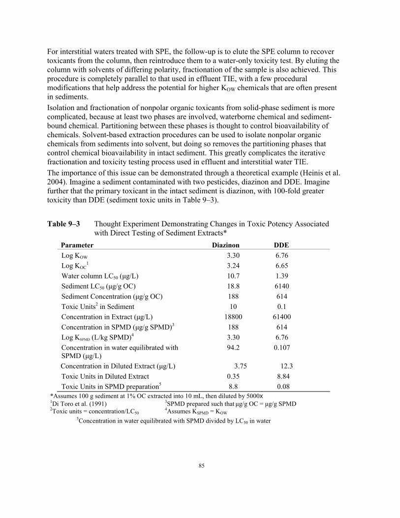
85

For interstitial waters treated with SPE, the follow-up is to elute the SPE column to recover toxicants from the column, then reintroduce them to a water-only toxicity test. By eluting the column with solvents of differing polarity, fractionation of the sample is also achieved. This procedure is completely parallel to that used in effluent TIE, with a few procedural modifications that help address the potential for higher KOW chemicals that are often present in sediments. Isolation and fractionation of nonpolar organic toxicants from solid-phase sediment is more complicated, because at least two phases are involved, waterborne chemical and sediment-bound chemical. Partitioning between these phases is thought to control bioavailability of chemicals. Solvent-based extraction procedures can be used to isolate nonpolar organic chemicals from sediments into solvent, but doing so removes the partitioning phases that control chemical bioavailability in intact sediment. This greatly complicates the iterative fractionation and toxicity testing process used in effluent and interstitial water TIE. The importance of this issue can be demonstrated through a theoretical example (Heinis et al. 2004). Imagine a sediment contaminated with two pesticides, diazinon and DDE. Imagine further that the primary toxicant in the intact sediment is diazinon, with 100-fold greater toxicity than DDE (sediment toxic units in Table 9–3).

Table 9–3 Thought Experiment Demonstrating Changes in Toxic Potency Associated with Direct Testing of Sediment Extracts*

Parameter Diazinon DDE Log KOW 3.30 6.76 Log KOC

1 3.24 6.65 Water column LC50 (μg/L) 10.7 1.39 Sediment LC50 (μg/g OC) 18.8 6140 Sediment Concentration (μg/g OC) 188 614 Toxic Units2 in Sediment 10 0.1 Concentration in Extract (μg/L) 18800 61400 Concentration in SPMD (μg/g SPMD)3 188 614 Log KSPMD (L/kg SPMD)4 3.30 6.76 Concentration in water equilibrated with SPMD (μg/L)

94.2 0.107

Concentration in Diluted Extract (μg/L) 3.75 12.3 Toxic Units in Diluted Extract Toxic Units in SPMD preparation5

0.35 8.8

8.84 0.08

*Assumes 100 g sediment at 1% OC extracted into 10 mL, then diluted by 5000x

1Di Toro et al. (1991) 3SPMD prepared such that μg/g OC = μg/g SPMD 2Toxic units = concentration/LC50

4Assumes KSPMD = KOW 5Concentration in water equilibrated with SPMD divided by LC50 in water

86

Assume that we then prepare a solvent extracted from this sediment, and then tested the extract for toxicity by adding a small amount to clean water. Because DDE has a higher (sediment organic carbon) KOC, the concentration ratio of DDE to diazinon in the sediment extract (and therefore in the water spiked with this extract) would be much higher than in the interstitial water. This change in relative concentration would then change the relative toxicity of the two chemicals in the fraction test; in fact, the fraction test would show toxicity due to DDE, with 25-fold greater potency than diazinon (extract toxic units in Table 9–3). The exact opposite situation existed in the intact sediment. So if one conducted a TIE on the extract spiked back into water, the conclusion would be that DDE was the primary toxicant in the sediment, which is wrong. To avoid this problem, one needs a method for testing sediment extract that preserves the differential partitioning behavior that controls bioavailability in the intact sediment. Such a method has been proposed by Heinis et al. (2004), wherein sediment extracts or fractions thereof are tested using a semipermeable membrane device (SPMD). SPMDs were originally developed for use as passive sampling devices for monitoring water column concentrations of bioaccumulative chemicals in the environment (Huckins et al. 1993). An SPMD is a length of polyethylene tubing containing triolein. In its deployment as a sampling device, chemicals from the water column partition into the SPMD in a ratio that is similar to the octanol-water partition coefficient (KOW). However, one can also drive this partitioning in reverse, by placing chemicals into the SPMD, then allowing those chemicals to partition out into the surrounding water. Because KOW is very similar to typical partition coefficients between water and sediment organic carbon (KOC), this partitioning is very similar to the partitioning that governs bioavailability in sediments. As shown by Heinis et al., one can therefore use the SPMD for sediment TIE by loading a sediment extract into an SPMD and placing it in water to equilibrate. In doing so, one essentially creates an exposure and bioavailability similar to that expected in sediment, and thereby overcomes the bioavailability problem. Table 9–3 shows how the same example would play out using an SPMD to expose organisms to the extract, and how it preserves the relative potency found in the intact sediment. The details for the SPMD method are provided in subsequent sections and by Heinis et al. (2004).

9.3.1 SPMD Method for Solid-Phase Sediments The SPMD method should be considered more as a general approach than a strictly defined method; it is likely that there are many variations of this approach that would yield useful results. To facilitate the implementation of this procedure in laboratories new to the method, the following sections give some specific parameters (e.g., SPMD size, etc.), but these should only be considered as methods that have been shown to work, not as the only methods that will work. The first step in the method is to prepare a solvent extract from the test sediment. Because in the context of a TIE the analytes of interest are not known and vary from sediment to sediment, it is not possible to have a single extraction procedure that is highly effective for every sediment and toxicant. In order to cover a variety of chemicals with a range in properties, we have used a mixed solvent system of hexane:acetone:dichloromethane in a 60:20:20 (v/v/v) mixture (referred to as “solvent mix” from now on). We have extracted sediment in batches of 40 to 100 g (air dry). The specific amount of sediment needed depends on the organic carbon content and the study design. It is best to consider the entire

87

procedure and back-calculate the amount of sediment that should be extracted. When larger amounts are needed, multiple aliquots of sediment are extracted and the extracts combined. Air-dried sediment is ground to a powder using a mortar and pestle, combined with an equal mass of anhydrous sodium sulfate, and extracted three times with 75 mL of solvent mix in a sonicating bath at 35°C. The combined extract is then dried by passing it through a funnel containing a plug of glass wool covered with a layer of anhydrous sodium sulfate. The extract is concentrated to a final volume of 40 mL in a 50°C water bath with a stream of dry nitrogen. SPMDs can be prepared in any length desired. In our work, we found that SPMDs as short as 10 cm long containing 0.1 g of triolein were effective; smaller SPMDs require less sediment extract, so we have adopted this size. Experiments conducted with different configurations suggested that maintaining a ratio of 0.1 g triolein for each 10 cm of polyethylene tubing yields partitioning behavior that best emulates KOW for the chemicals we have examined (Heinis et al. 2004). The next step is to solvent-exchange an aliquot of the extract into an aliquot of triolein, to be loaded into the polyethylene tubing. The calculation of how much extract to place in each SPMD depends on the characteristics of the sediment and the desired exposure. Different exposure concentrations can be achieved by loading the SPMDs with differing amounts of extract. Experimentally, we have found for several non-ionic organic chemicals that the partition coefficient between water and SPMDs (KSPMD) approximates KOW, a finding that is consistent with other literature data. Since the partition coefficient between organic carbon and water is also approximately equal to KOW, it follows that KSPMD is approximately equal to KOC. On that basis, the expected chemical exposure in sediment and in an SPMD preparation can be expressed relative to the mass of organic carbon in the sediment and the mass of the SPMD. For example, assume a test sediment with 1% organic carbon. Extracting 100 g of this sediment is the equivalent of extracting 1 g of sediment organic carbon. If one transfers this extract into an SPMD weighing 1 g (total, triolein + tubing), then the expected exposure in both preparations is the same (assuming KOC = KSPMD and 100% extraction efficiency from the sediment). We refer to this as a 1 x SPMD treatment. Placing the extract from 200 g of this sediment is equivalent to 2 g organic carbon (e.g., 200 g of sediment with 1% organic carbon); placing this extract in a 1 g SPMD would represent a 2 x SPMD treatment, or an exposure twice that expected in intact sediment. Using a volume of extract equivalent to 50 g sediment (0.5 g organic carbon into a 1 g SPMD would yield a treatment of 0.5 x SPMD (0.5 g organic carbon/1.0 g SPMD). The specific concentration to test depends in part on how toxic the test sediment is. If it is only marginally toxic, then it might be wise to test it at 2 x or more, to insure that it is still toxic even if there are some procedural losses. Alternatively, if a sediment is very highly toxic, it may be desirable to test it at lower concentrations. Since lower concentrations require increasingly small amounts of extract, conducting a series of decreasing concentrations of highly toxic sediments may be useful. One advantage of the SPMD method is that it allows the calculation of toxic units like those calculated for effluent TIE, because the organism response should be directly proportional to the concentration of chemical in the

88

SPMD. This is not necessarily the case for the dilution of contaminated sediment with clean sediment. To solvent-exchange the desired aliquot of sediment extract into triolein, combine the desired mass of triolein (e.g., 0.1 g for a 10 cm SPMD) with the appropriate aliquot of sediment extract, then reducing the mixture to a constant mass in a 50°C water bath under a stream of dry nitrogen. Determine the final mass of the triolein/extract mixture. Low-density polyethylene (LDPE) tubing, 2.5 cm wide with 100 μm thick walls (CIA Labs, St. Joseph, MO, USA), is initially cleaned by soaking it in a solution of hexane:dichloromethane (80:20, v/v) for 3 hours, air drying, and then drying under vacuum at room temperature for 18 hours. The exact procedure for loading and sealing the SPMD can vary, depending on the techniques and prior experience of the analyst. What follows is the method we have used successfully, but other methods that achieve the same end product could be used. The appropriate length of tubing (e.g., 10 cm) is cut off, flattened, then one end is heat sealed about 1 cm from the end (previous experimentation is required to determine the appropriate conditions for heat sealing such that a complete seal is achieved without burning a hole in the tubing). To provide a point of attachment to a support structure, we create loops of tubing at the ends of the tubing. This is done by doubling the 1 cm “tail” back on itself and heat sealing the end to form a loop. Any excess material can be trimmed off. The next step is to transfer a quantified mass of triolein/extract mixture into the SPMD. We accomplish this using a clean, empty beaker as a holder. Tare the beaker, then place the tubing in the beaker such that the open end of the tubing faces upward and about 1 cm above the beaker’s lip. Weigh the beaker and tubing to obtain the mass of the tubing. Open the end of the tubing by squeezing the sides together; the goal is to form an open, vertical column with the end of the tubing. Using a clean pipette or syringe, transfer the appropriate aliquot of triolein/extract mixture into the tubing, placing it as far down into the tubing as possible. It is important to keep the last 1.5 cm or so of the tubing clean and free of extract so that it can be heat sealed without loss. After the extract is transferred, weigh the beaker again to determine the exact mass of extract added. Remove the SPMD from the beaker and place it flat on clean aluminum foil. Using a glass rod, move the triolein/extract around in the tubing to obtain a reasonably uniform layer along the length of the tubing, being careful to exclude air and to keep extract away from the open end of the tubing. Heat seal the tubing about 1 cm from the end, then double it over and heat seal that end into another loop. The SPMDs are then placed in the test beaker. In our experiments, we have used a 600-mL beaker containing 300 mL clean water of a chemistry appropriate for the test organisms to be used. The SPMDs need to be situated in the test beaker to maximize the contact between the test water and the SPMD. We have accomplished this by creating a small rack out of stainless steel wire onto which the SPMD is placed in a zig-zag pattern (Figure 9–1a). The ends of the wire are left long enough to serve as handles for placing and removing the SPMD easily. For marine tests, bent glass tubing in approximately the same configuration is used to suspend the SPMD in the water column (Figure 9–1b).

89

Figure 9–1 Racks for Working with SPMDs. (a) Freshwater Stainless Steel Rack, and (b) Marine Glass Rack

a

b

The test beakers containing the SPMDs are then placed into a test system capable of maintaining the appropriate test temperature. In addition to treatments containing sediment extracts, control treatments should include a negative control with no SPMD, and a procedural control with an SPMD loaded with triolein only. The SPMD test is a water-column exposure; if the test organism requires a substrate, place a layer of clean, non-sorptive material such as clean silica sand on the bottom of the beaker. For H. azteca and C. dilutus, a 1 mm layer is sufficient; no substrate is necessary for L. variegatus. Commonly tested marine organisms (A. abdita, A. bahia, M. mercenaria, and C. volutar) require no substrate. We do, however, put a piece of black plastic under the test beakers to encourage A. abdita to stay at the test beaker bottom and not swim to the surface where they can be trapped by the water surface tension. To speed equilibration, each test chamber should have a small amount of aeration to very gently move the test solution in the beaker. We use a fritted glass dispersion tube, or small-bore tapered glass pipette delivering a very low flow of clean filtered air (e.g., 70 mL/min). The goal is to provide some movement of the water column without creating currents that would unnecessarily disturb the test organisms. Covers are placed over the chambers to reduce evaporation. Small water losses to evaporation or sampling can be replaced with clean water as needed during the exposure. Time required for equilibration depends on the chemical and the specifics of the chamber geometry and mixing. In most cases we have found that 24 to 48 hours of equilibration is sufficient to obtain at least 50% of the steady-state concentration, and typically much higher (Heinis et al. 2004). Unless the target analyte is known, there is no way to verify the degree of equilibration. After equilibration, test organisms are added and testing and observation proceeds according to standard procedures. Food can be added for those organisms and/or test durations

90

requiring it. Because the SPMD is a partitioning-driven system, chemical losses to volatilization, sorption, or uptake by test organisms are compensated for by additional chemical release from the SPMD. To date, we have successfully used H. azteca, C. dilutus, L. variegatus, fathead minnows, Japanese medaka, A. abdita, A. bahia, and M. mercenaria in this test system. Daphnia magna have also been used, but we have encountered sporadic difficulties with blank toxicity. These include longer-term (7- to 10-day) exposures sufficient to measure sublethal endpoints (growth) as well as survival (Heinis et al. 2004) When applying the SPMD method to evaluate nonpolar organic chemicals, a typical first step would be simply to extract the whole sediment and test the unfractionated extract at an appropriate concentration to verify that the toxicity can be removed from the extract and reintroduced via the SPMD. If so, this is strong evidence that the nonpolar organic toxicants are present at toxic concentrations in the sediment. However, because most sediments contain a very complex mixture of organic chemicals, gas chromatography-mass spectroscopy (GC/MS) analysis of an unfractionated extract is likely to produce an enormous number of chromatographic peaks, many of which overlap to a degree that confident identifications and quantifications are not possible. To address this problem, the initial extract can be fractionated, and the resulting fractions tested just as described. Because the analytes of interest are unknown, it is difficult to derive one specific fractionation procedure that is appropriate for all samples, and we do not yet have sufficient experience to recommend anything specific. In effluent fractionation, the fractions themselves are diluted into water for toxicity testing, which requires that the solvents used must be compatible with the test organisms. In the SPMD approach, the fractionation solvents are removed, so it is not necessary to restrict the range of solvents used for fractionation. As a first step, a separation based on polarity is a logical approach, such as an alumina column eluted with hexane, then a hexane-methylene chloride mixture (e.g., 50:50), then a methylene chloride-acetone mixture. This is only a suggestion; any number of other fractionations proposed in the literature could be used. We suggest that the initial fractionation consist of a relatively small number of fractions (e.g., 3 to 6) to help insure that the toxicants are not diluted beyond detection in the fractionation. In addition, the fractionation procedure should be amenable to processing the relatively large amounts of extract involved. Several procedures for fractionating sediment extracts can be found in the literature (Beg et al. 2001; Brack 2003; Maltby and Betton 1995; Marvin et al. 1999). Regardless of the procedure used, SPMD tests conducted on fractions should probably use relatively high concentrations to avoid losing detectable toxicity due to procedural losses and/or splitting of toxicants among multiple fractions. It is also essential to test procedural blanks for toxicity to insure that toxic artifacts are not being introduced.

9.3.2 Alternate Phase II Solid-phase Methods for Organic Compounds Large mesh resins such as Ambersorb 563 can be sieved from the sediments and eluted with organic solvents. Anderson et al. (2006a) reported using this method with field sediments and successfully recovering the toxicity in acetone fractions tested as indicated by both marine and freshwater amphipods. Chemical analyzes of those fractions showed the eluates to contain hydrophobic constituents including pyrethroid pesticides.

91

9.3.3 C18 Solid Phase Chromatography and Fractionation for Interstitial Water The solid phase extraction and elution procedures for interstitial water are parallel to those developed for effluent samples. In that method, the C18 SPE column is used to remove nonpolar organic toxicants from the effluent sample, which then is eluted with a series of methanol:water solutions with increasing polarity. This series culminates in a 100% methanol solution, which is the most nonpolar solution used. While this approach proved effective for effluent samples, sediments tend to accumulate even more nonpolar chemicals, such that 100% methanol is not sufficient to elute these chemicals from the SPE column. As a result, the major change in adapting the effluent SPE procedure for interstitial water TIE is to amend the elution sequence to include additional solutions that are less polar. Specifically, the 100% methanol fraction is replaced by 50% methanol/50% methylene chloride, and three additional 100% methylene chloride fractions follow. In addition, we removed some of the more polar solvent mixtures. This modified method generates a total of nine fractions (Table 9–4). While we have chosen this particular scheme, other combinations of solvent mixtures and columns may perform equally well (Anderson et al. 2006a). When choosing solvent mixtures, biological compatibility and/or the ability to exchange solvent mixtures for biologically compatible solvents should be kept in mind. Section 9.8.2 presents further considerations for choosing solvent mixtures and extraction schemes. Table 9–4 Composition of Nine Recommended Solvents and Water Combinations for

Eluting the C18 Column in Phase II Sediment TIE Composition of Eluting Solutions (% by volume)

Fraction Water Methanol Methylene Chloride

1 50 50 0 2 20 80 0 3 10 90 0 4 0 100 0 5 0 100 0 6 0 50 50 7 0 0 100 8 0 0 100 9 0 0 100

In order to recover sufficient masses of chemical for fractionation, testing, and chemical analysis, it is best to process a large volume (i.e., 1 L) of interstitial water. While this may be logistically daunting, it is better to invest the effort to obtain a sufficient volume of water than to not have enough water and fail late in the extraction process. In effluent TIEs, the SPE procedure is performed on a filtered sample. However for interstitial water TIEs, we don’t recommend the filtration of the interstitial water, because we have often found that this results in a nonspecific reduction in toxicity. The original purpose of filtration was to prevent plugging of the SPE column by particles. However, this same objective can be met through double centrifugation of interstitial water (Section 8), avoiding any effects of filtration on toxicity.

92

As in the original effluent procedure, we recommend that one 6 mL high-capacity C18 column be used for every 1000 mL of sample fractionated. Throughout this procedure we recommend a flow rate of 7 to 10 mL/min. The column is preconditioned by pumping 25 mL of 100% methanol through the column, followed by 25 mL of high-purity distilled water. At this point, 25 mL of dilution water is passed over the column, the last 10 mL of which is collected for a column blank toxicity test. Special care must be taken not to allow the column to become dry at any time during the conditioning procedure. One solvent must be added after another in such a way that precludes air passing through the column. After the column is conditioned, the elution blanks are collected (Table 9–4). Three mL (in two 1.5 mL aliquots) of fractions 1 through 9 (i.e., 50% methanol:water to 100% methylene chloride) is passed over the column and each fraction collected in separate analytically clean labeled vials. Each eluting solution is allowed to pass completely through the column before the next solution is added to the column. The column may go to dryness during this procedure. After the elution blanks have been collected, the column should be reconditioned with methanol and water; again, it is important not to allow the column to become dry during reconditioning. To extract the IW, 1000 mL of double centrifuged interstitial water is pumped through the column at a rate of 5 mL/min. Three 20 mL samples of the post-SPE column effluent are collected after 25 mL, 500 mL, and 950 mL of the sample pass through the column. These aliquots can be tested to monitor for the breakthrough of toxicity in the post C18 sample (USEPA 1991a; 1992b). After the entire sample has passed the column, it is allowed to go to dryness. If the column plugs and the entire 1000 mL cannot be processed, collect a 20-mL sample of the last interstitial water to pass the column and record the total amount passed through the column. If needed, the remainder of the sample can be processed using another column, prepared and blanked. The loaded column is now ready for elution. The column is eluted exactly as described for the collection of elution blanks. If more than 1000 mL of sample is being fractionated, and therefore more than one column is being used (or if more than one column was needed to process 1000 mL), then the complete procedure from preconditioning, collection of the elution blanks, reconditioning, and column elution is repeated for each column. Corresponding fractions from several columns may be combined at this stage, but dilution water blanks should be kept separate. The vials containing the fractions are sealed with perfluorocarbon or foil-lined caps and stored under refrigeration. Because methylene chloride has higher toxicity than methanol, the methylene chloride must be eliminated from fractions before toxicity testing of the fractions can take place. Because concentrations of the high log KOW toxicants may be diluted over several fractions, it is best to combine those fractions that contain 100% methylene chloride (fractions 7 through 9). Then, one can eliminate methylene chloride from this one combined fraction, and reduce the volume to 3 mL, as would be the case if a toxicant had eluted in only a single fraction (i.e., in an ideal situation). Eliminating methylene chloride from methanol or exchanging it into methanol is relatively easy because methylene chloride is more volatile than methanol and can therefore be removed from a mixture of these two solvents by evaporation under a stream of nitrogen. We

93

have found that this step is readily accomplished by combining fractions 7 through 9 for a total of 12 mL in a 50 mL glass centrifuge tube. To this is added another 12 mL of methanol and a perfluorocarbon-coated magnetic micro stir bar. The centrifuge tube is placed in a water bath at 50°C and stirred magnetically with a stream of nitrogen gently flowing over the surface of the solution. Alternatively, the sample can be placed in a Turbo-Vap™ evaporator (Zymark Corp., Hopkinton, MA, USA) set at 50°C. The Turbo-Vap system automatically blows a gentle stream of nitrogen over the surface of the sample, resulting in both evaporation and mixing, until it reaches a specified volume. After the volume of the solution is reduced to 3 mL, the sides of the tube are carefully rinsed with 3 additional mL of methanol and the volume is again reduced by evaporation to 3 mL. These repeated evaporations and additions of methanol ensure that the methylene chloride is eliminated from the fraction. If only a single fraction containing methylene chloride is to be tested for toxicity, then exchange into methanol can be easily achieved by using this procedure. In this case, however, 3 mL of methanol are added to the fraction, the volume is reduced to 3 mL, and sides of tube rinsed with another 3 mL methanol followed by a final volume reduction to 3 mL. Because organic toxicants in sediments tend to be more nonpolar than those in effluents, sediment nonpolar compounds may not be very miscible in methanol or aqueous solutions. Sometimes, if we try to force a high concentration of nonpolar compounds into a polar solvent, a biphasic solution or undissolvable material in the test fraction has resulted. One way to counteract this is not to bring the test solution down to a small volume; however, this may decrease the ability to concentrate the test extract. Another method is to choose a biologically compatible, yet more nonpolar, solvent. Both acetone and DMSO have been used in this way. Any procedure that involves combining fractions or exchanging methylene chloride with methanol or other carriers also must be performed with the corresponding elution blanks. In that way, any artifactual toxicity that is inadvertently introduced by these procedures can be detected in the blank. Toxicity testing of SPE fractions is performed as described in the general Phase II effluent method (USEPA 1992b). When concentrating toxic fractions for further chemical analysis by GC-MS, samples need to be transferred to a nonpolar solvent such as hexane or heptane. Samples to be analyzed by GC-MS will need to be dried with sodium sulfate to remove water before analysis. Fractions to be analyzed by HPLC need to be solvent exchanged to a polar solvent such as methanol, acetonitrile, or water. The above methods used for solvent exchange for toxicity testing can also be used here. Further reverse phase fractionation of SPE fractions by HPLC, including fractions 8 through 11 (combined or individually), can be carried out exactly as described in the general method (USEPA 1992a). Compounds that require methylene chloride for elution from C18 SPE columns can often be fractionated by HPLC using a water:methanol solvent gradient. We have found that high log KOW compounds elute in the 90 to 100% methanol portion of such an HPLC gradient and therefore would be found in the 90 to 100% methanol HPLC fractions. The 100% fractions, therefore, can be concentrated for GC-MS analysis by evaporative volume reduction. However, we have been unable to determine whether useful separations of high log KOW compounds can be achieved by reverse-phase HPLC fractionation.

94

GC-MS analysis of concentrated SPE and HPLC fractions is performed in the same manner as described elsewhere (USEPA 1992b).

9.3.4 C18 Fractionation Considerations As discussed in the previous section, many types of nonpolar organic compounds that accumulate in sediments are less polar than those typically found to be toxic in effluents. For example, we have identified toxic C18 SPE fractions containing benzenes, PCBs, PAHs, and long-chain aliphatic hydrocarbons from sediment interstitial water samples from the Illinois and Saginaw Rivers (Ankley et al. 1991; Schubauer-Berigan and Ankley 1991; Schubauer-Berigan et al. 1990). The recovery of these more nonpolar compounds is often not predictable from the C18 column. At times, these nonpolar compounds (e.g., PCBs) can be eluted in the 90:10 and 95:5 methanol:water solvent mixtures and further elution of the column with 100% methanol, 100% methylene chloride, and 100% acetone did not produce any additional toxicity (Ho et al. 1997). In other studies, we were unsuccessful in recovering nonpolar organics from the C18 SPE column using the methanol:water scheme recommended in the Phase II TIE manual (USEPA 1992b). Instead, we used an increasingly nonpolar methylene chloride:methanol elution series to extract the more nonpolar compounds that appeared to be causing the sample toxicity. A series of experiments performed with standards containing compounds with log KOW values ranging from 3 to 8 confirmed that C18 SPE fractionation techniques do not provide predictable recoveries or separations for more nonpolar compounds. We have observed that for compounds with log KOW values of greater than 5, the same chemicals may be recovered in both the 100% methanol fractions, and in the more nonpolar methylene chloride:methanol fractions. However, the same standard fractionated by HPLC shows that increasingly nonpolar compounds are sequentially recovered, and more predictably, in the more nonpolar fractions. HPLC methods have far greater separation ability than simple column chromatography. Differences in column packing and elution conditions most likely also influence the elution of nonpolar compounds. Alternatively, a normal-phase silica gel column fractionation may be used. Normal-phase packings generally do not sorb organic compounds to the same degree as reverse-phase packings. However, normal-phase fractionation generally requires elutions with solvents that are not biologically compatible (e.g., hexane, methylene chloride). These nonpolar solvents need to be exchanged into carriers that are more biologically compatible (e.g., methanol) before testing. Scrupulous use of operational blanks is critical for work with less biologically compatible solvents in order to detect any toxicity resulting from the use of these solvents.

9.4 Sulfide Sulfide is produced naturally in anoxic sediments by sulfate-reducing bacteria, but the amount of sulfide produced may be increased by anthropogenic additions that enhance microbial activity (e.g., nutrients). Sulfide is present in anoxic sediments in many forms, both dissolved forms in interstitial water and mineral forms such as sulfides of iron and other metals. While solid forms such as metal sulfides are not thought to be toxic to benthic organisms, free sulfide in the water column is quite toxic to many aquatic organisms (Broderius et al. 1977). Most benthic organisms used for sediment toxicity testing are naturally adapted to living in the oxic layer overlying anoxic sediments, or actually within

95

the anoxic layer using adaptations such as irrigated burrows to obtain the oxygen necessary to sustain life. In whole sediment flow-thorough test systems, sulfide toxicity is likely to be minimized due to volatilization and dilution. However, we have documented sulfide toxicity in whole sediment static, aerated test systems. Although some sulfide is dissipated through the mixing and handling of sediments during test preparation, enough can remain to cause toxicity if initial concentrations are high. Sulfide toxicity is also quite possible in interstitial water tests, where the interstitial water is isolated from previously anoxic sediment and the nature of the subsequent exposure does not allow test organisms to avoid exposure by the normal mechanisms (e.g., irrigation of a burrow with overlying water with low sulfide concentrations). While sulfide is typically oxidized over time when oxygen is available, it can persist for some time in isolated interstitial water even after it is oxygenated enough to allow toxicity testing. Sulfide toxicity in the water column increases with decreasing pH, and sulfide itself is fairly volatile, increasingly so at lower pH. If a graduated pH test has not already been conducted, it should be, with the expectation of increased toxicity with decreased pH and/or reduced toxicity with increasing pH. However, many of the conditions that produce high sulfide concentrations in interstitial water (anoxic sediments) may also lead to increased ammonia; therefore, it is also important measure ammonia and factor its concentration into the interpretation of the graduated pH test. It would be theoretically possible for the graduated pH test to show relatively little change in toxicity if toxicity were caused primarily by ammonia at higher pH and by sulfide at lower pH. Chemical analysis to confirm the presence and concentration of dissolved sulfide is both straightforward and an important piece of evidence for sulfide toxicity. Hydrogen sulfide can be measured using either a modified colorimetric method (American Public Health Association (APHA) 1992; Knezovich et al. 1996), which has a detection limit of 3 μg/L for total sulfides, or an ion selective probe (Orion Research, Cambridge, MA, USA) which has a detection limit of 20 μg/L. It is obviously important that the analytical method have sufficient sensitivity to detect concentrations of sulfide toxic to the test species. Although some toxicity data for sulfide are available in the literature, the ease with which sulfide is lost from test solutions can make sulfide toxicity specific not only to the organism, but also to the specific test system used to (e.g., beaker size and geometry, temperature, airflow). For this reason, when sulfide is suspected it is prudent to conduct a toxicity test with sulfide-spiked dilution water to confirm the concentrations of sulfide that are associated with toxicity. Sodium sulfide (Na2S) is an appropriate form of sulfide for spiking experiments. Sulfide concentrations should be measured at the start of the exposure and at relevant times during the exposure to document the rate of sulfide loss. The volatility of sulfide at reduced pH can also be used effectively to implicate sulfide as a causative toxicant in interstitial waters. As sulfide becomes more volatile with decreasing pH, toxicity caused by sulfide should be readily lost under aeration at low pH (see USEPA 1991b for detail on pH-adjusted aeration tests). One can also use high pH aeration tests to show that volatility is retarded at high pH. If high pH aeration is used, it is important that nitrogen be used as the sparging gas instead of air. Sparging with air can induce sulfide loss by both oxidation and volatilization. If reduction in toxicity is intended, then it doesn’t really matter the degree to which loss occurs by either mechanism. However, if retardation of

96

volatilization is the goal, then it is important that oxidation be minimized so that toxicity is not lost by that mechanism, with misleading results. While loss of toxicity with low pH aeration is consistent with sulfide toxicity, more definitive evidence can be obtained by using a toxicant transfer or “purge and trap” approach. This is described in detail in previous TIE documentation (USEPA 1991b). In brief, the interstitial water sample is acidified to pH 3 and then sparged with nitrogen. Again, it is important to use nitrogen for this procedure to avoid oxidation of sulfide. Gas from the sparging vessel is then passed through a liquid trap of dilution water adjusted to pH 9. Sulfide liberated from the interstitial water at low pH should be retained in solution with higher pH. Volumes of the sample purged should be established so that there is no dilution of the toxicity to below toxic levels even after accounting for the possibility of less than 100% recovery. Following sparging, the pH of the trapping solution is readjusted to the initial pH of the sample and tested for toxicity. Even better, a graduated pH test can be conducted on the trapping solution to demonstrate that the recovered toxicant has the same pH dependence as in the original sample. Sulfide concentrations should be measured in both the sample purged and in the trapping solution. A procedural blank should also be included. Because sulfide is both volatile and easily oxidized, it is also common for sulfide toxicity in interstitial waters to be transient (e.g., toxic when tested immediately after isolation, but not toxic when tested again one or two days later). In whole sediments where pH adjustments are difficult, the volatility of sulfide from test systems can be used as an additional line of evidence to identify the toxicant. We have found that with normal aeration (approximately 2 bubbles/sec) for 72 hours in our whole sediment small volume static tests, total sulfide levels decreased from about 10 mg/L to about 0.4 mg/L. The total sulfide LC50 for two amphipod species, R. abronius and E. estuarius are 1.60 and 3.32 mg/L, respectively (Knezovich et al. 1996). The benthic burrowing shrimp, C. crangon, has a total sulfide LC50 of 0.6 mg/L (Vismann 1996). Fish and epibenthic organisms tend to be more sensitive to sulfides; the mussel M. edulis and the sea urchin S. purpuratus have total sulfide EC50 of 0.1 and 0.19 mg/L (Knezovich et al. 1996). While this simple aeration method may remove sulfides to a level at which they do not cause toxicity to benthic organisms, the sensitivity of the specific test organisms should be confirmed.

9.5 Toxicity Caused by Major Cations and Anions In one instance, we studied a sediment that contained unusually high concentrations of calcium, sufficient to cause toxicity to mysids. Although this was a marine sediment, it is possible that something similar could occur in freshwater sediments as well, and in either case it could involve other common cations and anions such as sodium, potassium, magnesium, and chloride. Toxicity of freshwater effluents caused by high concentrations of cations and anions is not uncommon (Tietge et al. 1997). Although marine organisms are naturally adapted to saline waters, they too are sensitive to waters with cations and/or anions in ratios sufficiently different from those in natural seawater (Douglas and Horne 1997; Pillard et al. 2000). None of the solid phase sediment manipulations should be expected to remove cation imbalance toxicity. While it seems logical that cation exchange resin might affect major cations, the resin recommended for use in bulk sediment TIE procedures for metals was

97

specifically selected for having higher affinity for common heavy metal cationic metals as compared to major ions like calcium and magnesium. Moreover, the much greater concentrations required to cause toxicity from major cations are such that they would likely overwhelm the capacity of the cation exchange resin. And finally, cation exchange resin does not only remove cations; it exchanges them, so any sorption of one cation must be countered by release of another (sodium in the case of SIR-300 used as described in Section 7.2.4.1), which may cause problems of its own. In effluent or interstitial water TIE, toxicity due to major cations or anions will result in none of the typical Phase I manipulations reducing toxicity. The next step is generally to measure the concentrations of sodium, potassium, calcium, magnesium, chloride, sulfate, and alkalinity in the sample. For freshwater samples, conductivity alone may give some indication of elevated concentrations of major cations and anions, but this is not very diagnostic, as the toxicity of these ions is determined by the specific concentrations of individual ions, not by the more general property measured by conductivity (Mount et al. 1997). As an example, H. azteca can easily tolerate seawater at 20% salinity, but is still sensitive to toxicity from major ions in waters with different ion ratios (Ingersoll et al. 1992). In marine waters, ionic imbalance toxicity may or may not be accompanied by changes in salinity. If the imbalance is due to an excess of an ion, the salinity may change; if toxicity results from a change in the ion balance, no salinity change may be noted. If major ion analysis indicates something suspicious, the most straightforward approach is to create a mock sample by spiking dilution water (or DI water if necessary) with common salts (e.g., NaCl, Na2SO4, CaCl2) to create a sample with major ion chemistry matching that in the interstitial water under study. This sample is then tested for toxicity using parallel methods. In addition to a baseline test with interstitial water and the usual negative (dilution water) controls, one might also consider a treatment using another mock sample that has had any unusual characteristics adjusted. For example, in testing a marine sample with excessive calcium, create another spiked sample of comparable composition except for a more proportional calcium concentration. This provides some assurance that artifactual toxicity is not introduced in the process of creating the mock sample itself, which is a concern for marine organisms in particular.

9.6 Manipulations Addressing Selected Anionic Metals: Chromium and Arsenic

Chromium and arsenic are two metals/metalloids that can be of concern in sediments and occur (or can occur) as oxyanions. These metals are known to contaminate sediments around the United States (Becker and Long 2006; USEPA 2004) and world (Aboul Dahab and Al-Madfa 1997; Becker and Long 2006; Mirlean et al. 2003; Neff 1997; Stronkhorst and van Hattum 2003). Although chromium and arsenic are known sediment contaminants, the frequency with which they cause toxicity to benthic organisms is not well understood. In the aquatic environment, arsenic and chromium assume anionic form resulting from oxidation/reduction and pH conditions (Bodek 1988). Arsenic has four oxidation states (-III, 0, III, V) and occurs in water as anionic arsenates V (H2AsO4

- and HAsO4-2) and arsenites III

(H3AsO30 and H2AsO3

-) (Bodek 1988). Chromium has three oxidation states (II, III, VI) and occurs as anionic chromates VI (CrO4

-2, HCrO4, and Cr2O7-2) and in trivalent forms

98

(Cr(OH)30 and Cr(OH)4

-) (Bodek 1988). Among these different forms, the trivalent (III) forms of arsenic and hexavalent (VI) form of chromium are considered to be the most toxic (Berry et al. 2004; Neff 1997). For example, LC50s for hexavalent chromium for the marine amphipod A. abdita are reported to be 1,980 µg/L, and the LC50 to the mysid A. bahia is 2,030 µg/L (Berry et al. 2004; USEPA 1985b), while LC50 values for trivalent chromium are generally an order of magnitude greater (Berry et al. 2004; USEPA 1985b). For aquatic organisms, LC50s for arsenic do not demonstrate the large differences between forms as observed between chromium III and VI (Neff 1997). The LC50 for arsenite (III) is reported as 1,740 and 8,000 µg/L for the mysid and amphipod, respectively (USEPA 1985c) while the LC50 for arsenate (V) is 2,319 and 4,160 µg/L for mysids and amphipods, respectively. In sediments, because of changes in oxidation/reduction conditions, arsenic and chromium shift oxidation states and therefore toxicity. Under reduced sedimentary conditions, arsenic is present primarily in the III form (Neff 1997) and may be expected to demonstrate greater toxicity. However, arsenic will react with sulfur to form relatively insoluble and (possibly) nonbioavailable compounds (e.g., AsS, FeAsS, As2S3) (Neff 1997). Recently, Berry et al. (2004) and Besser (2004) reported on the environmental factors controlling chromium bioavailability and toxicity. Under reduced sedimentary conditions, chromium assumes the III oxidation state and correspondingly demonstrates less toxicity (Berry et al. 2004). For both arsenic and chromium, it is likely that at sufficiently elevated concentrations, and despite changes in oxidation state and presence of binding phases, toxicity to benthic organisms will occur. Because anionic metal toxicity in sediment is thought to be associated with concentrations of metals dissolved in the interstitial waters, TIE methods for these metals seek to reduce these concentrations. In an effluent TIE, Mount and Hockett (2000) used anion exchange resin columns (Amberlite IRA410, Continental Water System, Denver, CO, USA) to identify chromium as the cause of observed toxicity to freshwater species. Exchange columns can be prepared by placing 40 mL of resin in a 60-mL syringe. The resin packed column should be rinsed with 1 L of control water and then 1 L of test water at a rate of 25 mL/min. Ion exchange would also be likely to remove ions essential for freshwater test organism survival, so blank and effluent samples should be spiked with 10% (v/v) of mineral water (Perrier®) after ion exchange. Detailed procedures are described (Mount and Hockett 2000). Interstitial water TIEs involving chromium or arsenic have not been reported. For whole sediment TIEs, Burgess et al. (2007) recently reported on the use of anion exchange resins added directly to sediment as an approach for conducting TIEs for chromium and arsenic. Although these methods were developed for saltwaters and marine species (i.e., A. abdita and A. bahia), it is likely they will function in freshwater systems once tolerance data has been generated for freshwater species. Additions of anion exchange resins to whole sediments have been effective in reducing toxicity and dissolved concentrations of anionic chromium and arsenic. These resins consist of some type of silica or polymer structure coated with a specific functional group including positively charged dimethyl-, trimethyl- and proprietary amines (Burgess et al. 2007). Binding of the dissolved negatively charged metals to an anion exchange resin reduces the bioavailable concentration of metal. We have used SIR-700 for chromium and ASM-10-HP for arsenic (ResinTech, West Berlin, NJ, USA). These resins were found most effective among a small group of resins evaluated

99

by Burgess et al. (2007) including weak base (WBMP-HP) and strong base (SBMP1-TR) resins. Features of the resins that make them useful for this application include a very high affinity for metal anions of concern (e.g., chromium or arsenic) and low toxicity to sediment test organisms. Other resins, not yet evaluated, may also be effective for use in whole sediment TIEs. As noted above, the following method was developed for saltwater systems, however, the resins should also function in freshwater systems. Both resins, SIR-700 and ASM-10-HP, should be rinsed before use by combining resin with deionized DI water (approximately 1:4 v/v) in a beaker, swirling the mixture to thoroughly mix and resuspend the resin, allowing the mixture to settle (e.g., 1 min.), then decanting the water. This procedure is repeated two times for a total of three DI rinses. Next, the decanted resin is combined with four volumes of saline water (e.g., 30‰ natural seawater or 30‰ reconstituted natural seawater prepared from brine), and mixed as above two more times for a total of three saline rinses. We store the resin in saline solution from the last rinse for 24 hours at 4ºC in the dark before use. Prior to use, each resin is removed from the storage container (taking care to allow any excess liquid to drain via gravity), measured into aliquots appropriate to bring the test sediment to 20% resin (24 g resin-sediment mix/replicate), then transferred to the test sediments, and mixed thoroughly. This can be performed in batch mode by treatment or on each individual replicate. We prepare the sediment-resin mixture in batches and then add aliquots of the mixture to the individual replicates followed by overlying water. Sediments are then equilibrated for at least 24 hours before organisms are added. Both the test sediment and a procedural blank (using control sediment) are prepared and tested. The resins described by Burgess et al. (2007), SIR-700 for chromium and ASM-10-HP for arsenic, were shown to significantly reduce the overlying and interstitial water concentrations of arsenic and chromium, as well as several cationic metals including cadmium, lead and zinc and to a lesser degree, ammonia. Concentrations of a representative organic pesticide, endosulfan, were not significantly affected by the presence of the two anionic resins. Together, these results reinforce the need to conduct structured TIEs involving the different manipulations performed simultaneously. Using this structure reduces the possibility of misinterpreting results caused by a manipulation unexpectedly altering the bioavailability of an unintended sediment contaminant. Thus, reduction in toxicity by the anion exchange resin additions should be viewed as consistent with toxicity caused by either chromium or arsenic, but not conclusive evidence by itself. As with most tests, conclusions from individual tests should be viewed in the context of the results from the entire Phase I TIE. Like the cation exchange resin addition, the anion exchange addition involves a substantial physical dilution of the sediment; therefore, results of a sand dilution blank test should be considered. Although recovery of the sorbed metal from the resin has not been evaluated, it may be possible to sieve the resin(s) from the sediment at the end of the TIE using a 0.5 mm screen and then elute the resin with a strong basic solution to extract sorbed metals for later chemical analysis and testing. As noted, this aspect of the manipulation has not been evaluated but would be similar to the approach taken in Phase II with cationic metals (Section 9.2.7).

100 1

9.7 Phase II Approaches When No Phase I Manipulations Affect Toxicity As was found in effluent TIE, there are instances when no Phase I manipulations alter toxicity of the interstitial water or bulk sediment. Although initially frustrating, there are options for pursuing toxicant identification in such situations.

In general, there are three primary reasons why toxicity might not be affected by any Phase I manipulations:

• The concentration of toxicant is too great and overwhelms the toxicity reduction capacity of the otherwise applicable manipulations.

• The properties of the toxicant are such that no Phase I manipulations are effective. • There are multiple toxicants at work, such that reduction of one toxicant by a

manipulation is masked by the presence of another toxicant. Although which of these (or others) is responsible may not be known until after the toxicant(s) is ultimately identified, it is useful to keep these possibilities in mind while evaluating data and designing next steps. The order in which the suggestions are discussed does not reflect a particular priority for implementation, which would be sample specific. Instead, we encourage investigators to consider all of the suggestions and implement those that make the most sense in light of the particular circumstances. If high toxicant concentrations overwhelm a manipulation, this might sometimes be avoided by insuring that the sample being tested is close to its threshold for toxicity. Section 7 describes the pros and cons of sediment dilution; however, regardless of the disadvantages one often needs to dilute very toxic sediments in order to make any progress in identifying sediment toxicants. If no Phase I manipulations affect toxicity, the investigator might consider further diluting the sample and trying again. Of course, there is no point in conducting Phase I testing on a sample that is so marginally toxic that typical variations from random variability alone are sufficient to obscure a characterization pattern. Another possibility is to change the matrix of the test used in Phase I. Even though the Phase I methods for both bulk sediment and interstitial water contain manipulations targeting similar groups of toxicants, they are based on different approaches and use different amendments. As such, it is possible that a more interpretable characterization pattern might be obtained by using the approach not used initially (e.g., if whole sediment testing was used initially for Phase I, try an interstitial water Phase I, assuming the interstitial water is toxic). Some toxicants are such that no Phase I manipulation would be expected to affect their toxicity. Examples include toxicity from major ions and hexavalent chromium. While it can be nonproductive to begin chasing after isolated possibilities without a specific reason to suspect a particular toxicant, directly measuring concentrations of such toxicants may be warranted if there is reason to believe they may be present. It should also be kept in mind that some toxicants targeted by Phase I manipulations may not respond to those manipulations because of a matrix interference or other difficulty. Accordingly, it may be worth verifying that such toxicants are not the culprits. Examples that come immediately to mind are ammonia and common cationic metals (e.g., zinc, cadmium, lead, nickel, copper). Ammonia should be measured in interstitial water (see Section 8).

101 1

Cationic metals can be measured in bulk sediment, interstitial water, or via peepers (Berry et al. 1996; Serbst et al. 2003). If measured in bulk sediment, analysis should include AVS, and metals should be quantified as part of that extraction as “simultaneously extracted metals” (Di Toro et al. 1990; Hansen et al. 1996). Measuring sulfide may be warranted, particularly if the sediment sample or isolated interstitial water has a sulfide odor. Ruling out many of these “common” toxicants can narrow the universe of possible toxicants. There is some circumstantial evidence for polar organic compounds causing toxicity of field-collected sediments; however, no Phase I manipulations are targeted toward such compounds. Research with various column sorbents may be useful to remove and to isolate polar organics (la Farre et al. 2001). Effluent TIE work has identified various surfactants as suspected toxicants in water samples (Ankley and Burkhard 1992; Ankley et al. 1990a; la Farre et al. 2001). The behavior of surfactants or other polar organic compounds in sediment TIE has not been studied, but one might suspect that the toxicity of surface active compounds would be ameliorated considerably by sediment particles. We have conducted several bulk sediment TIEs on harbor sediments that are generally thought to be primarily contaminated with PAHs from petroleum, coal tar, or other oily wastes. In these studies, we have often observed that the coconut charcoal and carbonaceous resin treatments did not appreciably reduce or remove toxicity as might be expected for a nonpolar organic contamination such as PAHs. Our investigations into this phenomenon are ongoing, but we have strong circumstantial evidence that the reason may be that toxicity to H. azteca and C. dilutus was caused by the presence of a non-aqueous phase (an “oil”) rather than from direct toxicity caused by specific components, such as PAHs. One piece of evidence is that, when such sediments are treated with coconut charcoal, concentrations of PAHs in IW are greatly reduced, as are concentrations of PAHs in tissues of exposed organisms. These measurements indicate that PAH exposure is in fact being reduced by the manipulation, but it is just not reducing toxicity as one would expect. In separate experiments, we have spiked mineral oil (a refined oil containing alkane hydrocarbons, but not PAHs, and generally thought to be non-toxic) into sediments and have shown toxicity to H. azteca and C. dilutus at concentrations similar to the concentrations of solvent-extractable material (“oil and grease”) found in the harbor sediments. At the time of this writing, we are working on, but have not yet developed, a TIE manipulation to address the toxicity of non-aqueous phases, so we cannot offer specific guidance about how to demonstrate experimentally that non-aqueous phases are a cause of toxicity. In general, it appears that sediments with two or more grams of solvent extractable material per liter of sediment tend to have toxicity to H. azteca and C. dilutus with the characteristics described above. Note that we are normalizing the solvent extractable material to sediment volume rather than sediment weight, because we have found that this normalization correlates better with observed toxicity. As indicated above, we are continuing to work on this problem and will publish our findings as they become available. The majority of the solid-phase TIE manipulations have been developed using the premise that reducing chemical activity (concentration) in the interstitial water will reduce toxicity. While toxicity via sediment particles is indirectly addressed because chemical sorption to particles is influenced by chemical concentration in interstitial water, toxicity due to particle ingestion (of either metals or organics) is not overtly addressed by the solid-phase TIE

102 1

methods presented here. Therefore, it is conceivable that organisms susceptible to toxicity via ingestion of sediment might not be addressed by these methods. The extent of this potential shortcoming is not clear, as one of the organisms used successfully with these methods (C. dilutus) feeds by ingesting sediment, particularly in fine grained sediments (Sibley et al. 1998). An approach that we have not yet explored may be to increase the equilibration time of the sorbent used in whole sediment exposures. While this may have limited success for cation resins designed to sorb metals due to relatively fast equilibration times, it may increase the effectiveness for organic sorbents such as PCC and carbon-based resins which have slower equilibration times with organic toxicants. Another approach to identify toxicants when traditional methods have not succeeded may be to conduct interstitial water manipulations in conjunction with pH adjustments. The original Phase I TIE methods for effluents included several manipulations using pH-adjusted (acidic and basic) samples. With the exception of the graduated pH test, these pH-adjusted manipulations were not included in the initial Phase I methods for either chronic TIE on aqueous samples or the interstitial water methods described in this document. This change was based on two factors:

• Experience gained since the original development of the aqueous Phase 1 methods, which suggested than many toxicants could be characterized without the additional pH-adjusted tests; and

• The logistical constraints of conducting additional tests with chronic test methods or, in the case of sediments, the substantial effort required to isolate sufficient additional interstitial water to perform the additional tests

While we stand by this reasoning in general, there are toxicants that respond to altered pH alone or in combination with aeration, filtration, or SPE manipulations, suggesting that these might be considered when the manipulations conducted at ambient pH do not yield sufficient information. The methods for these pH adjusted manipulations are described Section 9.8. The presence of multiple toxicants can confound attempts to characterize toxicity, particularly if the toxicants have different physical or chemical properties and therefore respond differently to Phase I manipulations. For example, consider a hypothetical interstitial water with 10 toxic units of zinc and 2 toxic units of ammonia. In this scenario, an EDTA test performed at a 100% or 50% interstitial water concentration would not be expected to remove sample toxicity because even with the zinc chelated and detoxified, there would still be a toxic amount of ammonia present. If, however, this sample were diluted sufficiently to reduce the ammonia concentration below its toxicity threshold (e.g., 25%), the remaining toxicity would be attributable to zinc only, and would be removed by EDTA treatment. This is another reason why diluting the sample to near its threshold for toxicity can be important in identifying the causes of toxicity (or one of them, in this case). It’s worth noting that diluting a sample to eliminate the effect of one toxicant does not solve the entire problem. That is, even though one of the sediment toxicants is identified, there is another toxicant that remains unknown. However, it is generally far easier to identify a second toxicant once the first is known. For example, in our hypothetical case, once zinc was

103 1

identified, we might be able to do a Phase I characterization on a sample that had EDTA added (to eliminate the zinc toxicity) in order to characterize the second source of toxicity. If the multiple toxicants are present at a more equal potency, then dilution will not solve the problem. In this instance, use of multiple and/or sequential manipulations may be useful (Ho et al. 1999a; Phillips et al. 2003; Science Applications International Corporation 2003). For example, if both ammonia and nonpolar organic toxicants were present at roughly equal potency, it is likely that no one manipulation would remove toxicity. However, testing SPE-treated interstitial water in a graduated pH test might reveal the roles of both toxicants. Sequential manipulations can also be useful when the manipulations are not entirely toxicant specific; for example, U. lactuca in aqueous solutions removes both ammonia and some nonpolar organic chemicals. To distinguish between the two and determine the contribution of each of these to overall toxicity, we passed the sample through a C18 column and divided the treated sample into two aliquots. One of these was tested for toxicity without further manipulation, while the other was treated using U. lactuca and then tested. Any difference between the baseline and the post-C18 toxicity is most likely due to organics, while the difference between the post-C18 and the Ulva treatment toxicity is likely due to ammonia (Ho et al. 1999a). Another example is discrimination between the effects of lead, zinc, copper, and ammonia by comparing the results of the graduated pH, sodium thiosulfate, and EDTA tests (Schubauer-Berigan et al. 1990). Such distinctions are possible because these compounds behave uniquely when exposed to combinations of these tests. These responses are summarized in Table 9–5.

Table 9–5 The Effect of Graduated pH, Sodium Thiosulfate, and EDTA on Ammonia, Copper, Lead, and Zinc Toxicity

Toxicity Response Under

Toxicant Reduced pH EDTA Addition Thiosulfate Addition Ammonia Decreases No change No change

Copper Increases Decreases Decreases Lead Increases Decreases Little/no change Zinc Decreases Decreases Little/no change

9.8 Manipulations Under Acidic and Basic Conditions We recommend that, for interstitial water TIE, initial Phase I testing omit the pH-adjusted manipulations that are included in the acute TIE methods for aqueous samples. While we believe these additional tests are often unnecessary, they may provide important clues in cases where the initial Phase I characterization does not yield a clear pattern. Some toxicants undergo irreversible changes under acidic or basic conditions. For example, malathion degrades under basic conditions and its toxicity is therefore reduced or removed simply by temporary adjustment of the sample to basic pH. In addition, some toxicants undergo reversible changes that alter their response to aeration or SPE. Examples here include sulfide

104 1

(more volatile at reduced pH) or an ionizable organic chemical that becomes more nonpolar (and therefore amenable to SPE) under acidic or basic conditions. Extreme pH manipulations are applicable only to interstitial water TIE; attempts to dramatically change the pH of whole sediments cause dramatic changes in sediment properties and associated artifactual toxicity. Acidifying sediments will likely mobilize large amounts of metals from otherwise nontoxic mineral forms, reactions that will not be reversed when the sediment is neutralized. Even within interstitial water TIEs, extreme pH manipulations are generally used for freshwater samples, as comparable manipulation of seawater can lead to precipitation of native ions and subsequent artifactual toxicity. Even if pH-adjusted manipulations do not directly lead to the identification of the causative toxicant(s), they can be very useful in ruling out toxicants and/or identifying characteristics that can be used in later confirmation studies. For example, if aeration at low pH does not affect toxicity, then it is unlikely that sulfide is a cause. On the other hand, if low pH aeration does reduce toxicity of the interstitial water, then one can expect that the true toxicant will show the same behavior when spiked into clean water and subjected to this manipulation. In freshwater samples, pH 3 and pH 11 adjustments are made by adding either 1.0, 0.1, or 0.01 N concentrations of HCl and NaOH to the interstitial water or elutriate sample. Follow the procedures and precautions noted elsewhere (USEPA 1991a). In general, it is desirable to use the most concentrated acid or base that one can while still maintaining control of the pH adjustment so as to minimize dilution of the sample. Table 8-2 gives the sodium chloride tolerances of H. azteca and L. variegatus, which may be used to determine whether the amount of sodium chloride resulting from the acid/base adjustments is sufficient to cause toxicity. Comparable tolerance values for C. dubia and fathead minnows are given (USEPA 1991a). As described for effluent TIE, when performing manipulations under acidic and basic conditions, it is important that there be an aliquot of sample that is pH-adjusted but not manipulated further in order to understand the effect of pH alone. If this is not done, one cannot know whether it was the pH adjustment alone, or the combination of pH adjustment with additional manipulation that affected toxicity. Accordingly, after the pH adjustments have been made, aliquots of pH-adjusted solutions are set aside for testing that involves pH adjustment alone, pH adjustment plus SPE, and pH adjustment plus aeration.

9.8.1 Aeration After pH adjustment, the aeration test is performed as described in Section 8.3.2 and in the effluent TIE guidance (USEPA 1996). Briefly, 30 mL of pH-adjusted sample and the corresponding blank are placed into separate 100 mL graduated cylinders and aerated for one hour. The rate of aeration should be vigorous (e.g., 500 mL/min) and equal among all treatments. The pH of each cylinder should be checked and readjusted with 0.01 to 1 N HCl or NaOH to the desired pH midway through the aeration procedure. After one hour of aeration, the sample should be removed from the aeration vessel and transferred to a clean beaker using a siphon or pipette to prevent any dissolving of sublated compounds into the sample. The different pHs not only affect the ionization state of polar toxicants, thus making them more-or-less volatile, but also affect the redox potential of the system. If toxicity is reduced by air sparging at any of the pHs, the presence of volatile, sublatable, or oxidizable

105 1

compounds is suggested. The role of oxidation can be evaluated by conducting an aeration test using nitrogen instead of air.

9.8.2 C18 Reverse-phase Solid-phase Chromatography By shifting ionization equilibria at the low and high pHs, the SPE column also can be used to extract organic acids and bases that are too polar to be extracted at the initial pH (pHi). The procedures for the pH-adjusted C18 extractions are identical to those for the pHi C18 manipulation described in Section 8. The C18 column packing is not stable at pH 11, so the pH 11 sample and its corresponding blank should be adjusted to a pH of 9 before passage through the SPE column. Some columns are designed to be stable at pHs up to 12 (Agilent Zorbax Extend-C18, Agilent Technologies) but we have not evaluated these columns for their efficacy or compatibility with biological testing. After conditioning and blanking the column, the pH adjusted samples are extracted as described previously. The post-column samples and blanks are then tested for toxicity as described in Section 8.3.3. If SPE removes toxicity, the resulting fractions and corresponding blanks are tested for toxicity. Fractions can be screened for toxicity initially by testing at a high concentration only; subsequent tests can evaluate dilutions of toxic fractions to quantify toxicity as necessary. If SPE removes toxicity under acidic or basic conditions, but not at pHi, involvement of an ionizable organic toxicant may be suspected. Since ionizable toxicants often show pH-dependent toxicity, it is important to keep this behavior in mind when conducting TIE testing. For example, if the pH of the dilution water is very different from the unaltered interstitial water, it is very possible that the toxicity of the causative toxicants may be different. Accordingly, be certain that the pH is carefully monitored and controlled to the extent possible when assessing ionizable toxicants. It is common for the pH of samples previously subject to pH manipulation to drift during testing in a manner different from the unaltered interstitial water. Again, great care must be taken to monitor these changes so their potential effects can be factored into data interpretation.

9.9 Phase II Summary The overall objective of Phase II is to develop enough evidence to be confident in identification of a toxicant (or group of toxicants). Certainly, methods other than those covered here can be used to develop that evidence. These may include manipulations for specific toxicants such as

• Methods that enhance or decrease the toxicity of pesticides such as temperature manipulation, addition of piperonyl butoxide and addition of esterases (Amweg et al. 2006; Ankley et al. 1991; Bailey et al. 1996; Phillips et al. 2004; Wheelock et al. 2004; Wheelock et al. 2006)

• Other sorbents that may separate toxicants using different properties (Anderson et al. 2006a; Cornelissen et al. 2001; la Farre et al. 2001; Petrovic et al. 2003; Phillips et al. 2004; Thomas et al. 1999; Waller et al. 2005)

• Novel extraction methods (Campbell et al. 1992; Deacon et al. 1991; Dumont and Fritz 1995; Hennion and Pichon 1994; Pichon et al. 1996; Waller et al. 2005)

• Enzymatic or protein assays for specific compounds (Moshe and Auslander 2005)

106 1

• Use of novel experimental protocols for distinguishing between toxic stressors (Anderson et al. 2006b)

Other references containing examples of TIEs include the Water Research Federation Report (Anderson et al. 2006a), the Naval Facilities Engineering Service Center guide (Science Applications International Corporation 2003), and the summary of the workshop held by the Society of Environmental Toxicology and Chemistry (Norberg-King et al. 2005). After completion of Phase II and if the objectives of the research require further confirmation, the investigator should feel confident with information from Phase II to move to Phase III confirmation.

107 1

10 Phase III Sediment TIE Methods As in effluent TIE, the purpose of sediment Phase III testing is to confirm that the suspected toxicant(s) identified in Phase II is(are) in fact the causative toxicant(s), and that all of the toxicity is accounted for. In addition, Phase III methods for sediment TIE may also involve demonstrating that the causative toxicant identified using interstitial water TIE is in fact the causative toxicant in bulk sediment tests. Failure to conduct adequate confirmation could be potentially disastrous, particularly if important decisions concerning remediation are to be made based on TIE results. Phase III is not a cookbook exercise wherein a standard set of tests is conducted and the results interpreted in a routine manner. Rather, it is a weight-of-evidence analysis, the extent of which depends on the consistency of the information obtained, and its sufficiency to support follow-on actions. In cases where important environmental and social decisions are contingent solely on TIE results (e.g., extensive remediation), evidence approaching certainty should be achieved. If, however, TIE results are themselves only one line of evidence in a larger risk assessment, then a lower degree of certainty may be appropriate. It is important to reiterate a point made in the Phase II discussion (Section 9), that the nature of TIE is such that one cannot “prove” that a particular toxicant is in fact the true toxicant. Instead, one simply collects enough supporting evidence (and, presumably, a lack of contrary evidence) sufficient to support the decisions to be made. Many of the approaches and issues involved in toxicant confirmation are already discussed in Phase III documents for effluent TIE (USEPA 1993a). Analysts conducting Phase III for sediments should already be familiar with those discussions. The text that follows focuses primarily on special considerations for conducting Phase III on sediments.

10.1 Defining the Objectives of Phase III Confirming the identity of a causative toxicant can be thought of as having two elements:

• Was the identification of the causative toxicant in the study sediment itself correct? • If so, is it appropriate to extrapolate that finding to a larger body of samples, either

spatially or temporally variable? The first of these is always important, while the importance of the second is situation-specific. As described throughout this document, sediment TIE may be performed using either solid-phase or interstitial water techniques. Because there are known differences in how toxicants and/or organisms may react in solid-phase versus interstitial water testing, it is important to insure that the TIE results are applicable to the actual management question. In most assessment situations, management of contaminated sediments will be based on the expected effects of bedded sediments. And, in general, an investigator might presume that solid-phase sediment toxicity tests might correspond better with the expected toxicity in situ, since the nature of the exposure is more comparable to field conditions. Thus, particularly when sediment toxicants were identified using interstitial water methods, it can be very important to verify that those same toxicants are responsible for the toxicity measured in solid-phase tests. This will not always be the case; for example, ammonia is apparently much

108 1

more toxic to Hyalella in water column tests (as in interstitial water) than in solid phase tests due to differences in exposure (Whiteman et al. 1996). In effluent TIE, an important component of Phase III is to determine whether the cause of toxicity identified in one sample is the ongoing source of toxicity in samples collected over time. There are cases in which sediment toxicants might be temporally variable, such as pesticide contamination associated with episodic applications or runoff events, or seasonal variation in sulfide or ammonia production from changes in microbial activity. However, most sediment contamination problems are the result of historical or ongoing pollution events, and tend not to be temporally variable. Nonetheless, a question of interest in sediment TIE might be whether the same toxicant is causing toxicity over a broader assessment area—particularly true in complex settings such as industrialized harbors, where there may be many different sources of contamination that vary in spatial intensity. While Phase III is distinct from other phases in concept, it may not be as distinct in terms of data collection and/or temporal sequencing of experiments. For example, in Phase II, we discuss many different approaches and manipulations that might be used to evaluate different types of toxicants. Depending on the path chosen, the amount of data generated in Phase II may vary. However, the body of data collected is part of the evidence that will inform Phase III in regard to the likelihood that the candidate toxicant is in fact the true toxicant. Moreover, it may be appropriate in Phase III to conduct additional Phase II manipulations relevant to the suspected toxicant in order to bolster the evidence for a particular toxicant.

10.2 Solid-Phase Versus Interstitial Water Testing Understanding the relationship between toxicity in solid-phase and interstitial water tests can be an important part of confirmation. As discussed in Section 6 on TIE study design, if the methods used in the toxicity test that determines the need for the TIE are different from those used in the actual TIE (e.g., solid-phase versus elutriate, or use of different test species), it is important that confirmation studies be conducted to connect the TIE findings with the endpoints of interest to the assessment issue at hand. As an example, if an interstitial water TIE implicated cadmium as a causative toxicant, then it might be prudent to conduct solid-phase manipulations using sulfide addition and cation exchange resin addition, to demonstrate a consistency of the solid-phase response with the interstitial water response. Even if the endpoint of interest is solid-phase toxicity and the TIE was conducted using solid-phase methods, conducting experiments with interstitial water can provide valuable information and the additional weight of evidence necessary to support confirmation. Using the example in the previous paragraph, where sulfide addition and cation-exchange resin removed toxicity, we might conduct an EDTA test on interstitial water to help reinforce a diagnosis of metal toxicity. The results of such experiments must be considered carefully. In this example, if EDTA also removed toxicity, it reinforces (but does not prove) that metals are the cause of toxicity. If EDTA does not remove toxicity, it could mean that metals are not the cause of toxicity, though not necessarily. Suppose this sediment had both ammonia and cadmium contamination and was toxic to H. azteca in the solid phase, and toxicity was removed by sulfide addition and cation-exchange resin. If we tested the interstitial water using the EDTA procedure, we might find that toxicity was not removed, not because cadmium was not the toxicant in the solid phase, but because the ammonia had greater effect

109 1

on the amphipods in the interstitial water test. These odd outcomes may not be the rule, but the investigator must keep them in mind as data are interpreted. For this example with cadmium and ammonia, additional TIE manipulations could quickly establish the role of ammonia in producing the seemingly anomalous result. This also emphasizes the importance of always measuring ammonia in interstitial water, because it is commonly elevated in anthropogenically influenced sediments, and because it is known to cause differing toxicity to some species in solid-phase versus interstitial water tests.

10.3 Predicting Chemical Toxicity in Sediments Somewhere in the process of toxicant identification or confirmation, it is generally necessary to estimate the toxicity of a candidate toxicant in sediment. This is an element of both determining whether a particular toxicant is a plausible cause of toxicity, as well as forming the basis for toxicity correlations as described later on (see Section 10.4). In effluent TIE, the potency of candidate toxicants is usually determined via literature data for water column toxicity tests, or by direct toxicity testing in dilution water and/or the effluent matrix. For sediments, the prediction of chemical concentrations that cause toxicity is more complicated. For interstitial water studies, the same general approach as is used for other water samples can be used. The primary concern is that the composition of interstitial waters is often very different from typical surface waters; specifically, dissolved organic matter tends to be much greater, as does water hardness (for freshwater sediments). These differences in the test matrix can have significant effects on the toxicity of both organic and inorganic toxicants. Ideally, we prefer to test candidate toxicants in the same matrix, less the native chemical. For nonpolar organic chemicals, this can be approximated by testing SPE-treated samples (i.e., spike neat chemical back into interstitial water after treatment with SPE). For metal toxicants, this approach has greater uncertainties, as ion-exchange columns might alter the general ionic composition of a sample, which would in turn alter the toxicity of the spiked metals. Another possibility is to spike chemical into interstitial water extracted from a site sediment with similar characteristics, but with much lower concentrations of the candidate toxicant and no intrinsic toxicity. Several sources have published sediment quality guidelines, giving chemical concentrations that are correlated to the presence of biological effects (Becker et al. 1990; Long et al. 1995; Swartz 1999; Wenning et al. 2005). Many of these, such as the ERL/ERM, TEL/PEL, PEC/NEC, AET, and others are developed from empirical correlations between measured concentrations of chemicals in sediments and observed toxic effects. While these guidelines have utility in sediment assessment, they are not based on cause-effect relationships between individual chemicals and should not be used in TIEs as a basis for predicting toxicity or calculating toxic units. For nonionic organic chemicals, the equilibrium partitioning (EqP) theory offers an approach for estimating the concentration of chemicals in sediment that would cause toxicity. This approach assumes that organic carbon in the sediment is the primary phase controlling bioavailability of nonionic organic chemicals to benthic organisms, and that the potency of sediment exposure is proportional to the concentration of chemical in the interstitial water.

110 1

Note: This does not mean that interstitial water is the only route of exposure, only that the aggregate toxicity of exposure to the sediment is indicated by the chemical concentration in interstitial water.

The concentration in interstitial water can be predicted from the organic carbon partition coefficient (KOC). Although specific characteristics of a sediment can cause KOC to vary, the default assumption is that KOC will be very close to the octanol-water partition coefficient (KOW). A general relationship of KOC to KOW has been proposed (Di Toro et al. 1991): log (KOC) = 0.00028 + 0.983 log (KOW) The units of KOC and KOW are L/kg. The relationship between chemical concentration in the solid phase and interstitial water (at equilibrium) is Csed dwt / fOC = Ciw * KOC where Csed dwt is the dry-weight normalized chemical concentration, fOC is the fraction of the sediment dry weight composed of carbon (e.g., 5% organic carbon is fOC = 0.05), and Ciw is the chemical concentration in interstitial water. By setting Ciw equal to the concentration that causes toxicity in a water column test, we can calculate the sediment concentration that would be predicted to cause equivalent toxicity to the same species in a sediment exposure. For example, assume we are evaluating the potency of DDE, with a log KOC of 6.65 and an LC50 for H. azteca of 1.66 μg/L (Holm-Hansen and Booth 1967). Inserting these values into equation 11-2 yields a sediment concentration of about 7400 μg/g organic carbon, or 74 μg/g dwt at an organic carbon content of 1%, as the sediment concentration expected to cause 50% mortality for H. azteca. While this calculation makes a number of assumptions, it can serve as a starting point for addressing the likelihood that a given chemical concentration could be responsible for toxicity in a given sediment. The partitioning part of this calculation can be spot checked by measuring chemical concentration in both bulk sediment and interstitial water in the sample of interest. The applicability of EqP for predicting toxicological response for a given species and chemical can be evaluated by conducting tests with spiked sediments in the same test system as is used for the TIE. For cationic metals such as cadmium, zinc, copper, lead, nickel, and silver, it is believed that partitioning is also a significant influence on toxicity, but the primary partitioning phase in anoxic sediments is acid-volatile sulfide (AVS) with additional influence exerted by organic carbon (see Section 9 and (USEPA 2005) for additional details). We would generally not expect to find acute metal toxicity exerted in sediments where either the summed concentrations of simultaneously extracted metal do not exceed that of AVS, or the concentrations of metals measured in interstitial water are below toxic concentrations. Because AVS and total organic carbon (TOC) vary widely in sediments, and because total metal concentrations can be influenced by relatively non-labile mineral forms, the dry weight metal concentrations that would be associated with toxicity can vary widely, and are therefore a poor basis for deciding whether a particular metal is a causative toxicant.

10.4 Correlation Correlation is one of the most commonly used confirmation approaches, wherein observed toxicity in a series of samples is regressed against expected toxicity due to measured concentrations of the suspect toxicants. Correlation is a very powerful Phase III procedure;

111 1

however, for this approach to be successful, there must be a range of samples with sufficiently different toxicities to develop a meaningful relationship among them. With effluents, correlation is often achieved by sampling over time; for sediments, temporal sampling will probably not give the variability desired, except in certain cases where seasonal variation in contamination occurs—e.g., seasonal agricultural runoff of relatively nonpersistent pesticides (Chandler and Scott 1991), biologically generated ammonia, or sulfide. For the majority of sediment assessments, the best strategy for maximizing variability is not by sampling over time, but by collecting sediment samples over a gradient of contamination. We have usually used horizontal distribution to generate such a gradient, but it is possible that vertical gradients in contamination might also be used. Depending on the characteristics of the study site, covariation of sediment contaminants may be an important influence on correlation analyses. For example, in some cases sediment contamination is the result of contaminant release from a single discharge or activity, decreasing in intensity with distance from that source. While this can provide a concentration gradient with respect to the candidate toxicant, it is often the case that many contaminants associated with that source follow the same gradient. As such, a correlation between the candidate toxicant and actual measured toxicity may occur, even if the identified toxicant is not the true cause of toxicity. On the other hand, complex sites with many sources of contamination can create the opposite problem. If a harbor contains many sources of contamination at levels sufficient to cause toxicity, then a gradient in concentration of the candidate toxicant may overlap with areas having toxicity caused by other chemicals. This could result in a poor correlation between observed and predicted toxicity across the gradient, even if the initial identification was correct. This is not intended to discourage investigators from using correlation approaches, but to emphasize that the interpretation of such correlations (or lack thereof) can be complex. The existence of a correlation does not, by itself, imply a correct identification, nor does a poor correlation necessarily imply an incorrect one. The general application of the correlation approach to interstitial water or elutriate samples is essentially the same as described for effluents; several examples are available in the literature (Figure 10–1; Amato et al. 1992; Ankley et al. 1990c; USEPA 1989b). Applying correlation to whole sediments has the additional wrinkle that the testing of sample dilutions to determine toxic units in the sample is not straightforward. While sediments can be diluted to reduce toxicity in general, the rate at which toxicity is diluted is not necessarily proportional to the mass or volumetric dilution; in other words, combining a toxic sediment with an equal volume of a control sediment does not necessarily (or even typically) yield a sediment with half the toxicity of the original. Alternatively, one may have two sediments with equal toxicity from the same chemical, but have different toxicity when each is diluted by 50% by the same sediment.

112 1

Figure 10–1 Correlation of Concentrations of Ammonia in Sediment Interstitial Waters from the Lower Fox River/Green Bay Watershed, with Toxicity of the Samples to Fathead Minnows and C. dubia*

Source: (Ankley et al. 1990c) *Toxicity expressed as TU (100/LC50 or 100/EC50) for (a) 96-hour fathead minnow mortality, and (b) 48-hour C. dubia mortality. When no mortality was observed, a value of 0 toxic units was assigned. In the two instances in the C. dubia test in which less than 50% mortality occurred at an interstitial water concentration of 100, a value of 0.5 TU was assigned.

For this reason, toxicity correlation plots are generally restricted to plotting survival on the y-axis (instead of toxic units, which are normally used in effluents). This greatly limits the dynamic range of contamination that can be effectively evaluated, since once 100% effect is reached, all samples with higher contamination are expected to yield the same result. Another complication lies in the x-axis of the correlation plot, which typically displays either toxic units or chemical concentration. Because bioavailability of chemicals can vary among sediment samples, the expression of contamination used for the x-axis must reflect contaminant bioavailability, not only concentration. For this reason, the x-axis should generally be expressed as organic-carbon normalized concentration for nonpolar organic chemicals, SEM-AVS for cationic metals (with a possible additional correction for organic carbon). See USEPA (2005) for chemical concentration in interstitial water–applicable to both organic and inorganic toxicants. For both sediment and effluent TIE, the degree of correlation that constitutes confirming evidence is debatable. Typical statistical expressions such as correlation coefficients are often calculated, but they are of limited use in defining adequacy, because their values are determined not only by the relative agreement between predicted and observed toxicity, but also by the magnitude of the contamination gradient studied. In addition, linear models of correlation may not be appropriate for graphs of contamination versus biological effect (e.g., survival), which can be expected to assume a sigmoidal shape and may require nonlinear regression techniques. Also important to consider is the weight of supplementary evidence.

113 1

For example, if there is a comparatively poor toxicity correlation over a limited contamination gradient, but there is other strong evidence from other experimental approaches that the identification is correct, then we might still conclude that the toxicant has been confirmed. No simple rules can substitute for appropriate professional judgment and sound scientific argument in evaluating the adequacy of confirmation data.

10.5 Spiking Confirmatory evidence can also be obtained through a number of approaches involving spiking samples with the suspect toxicant(s). In general, if the investigator notes an increase in the toxicity of a sample in the same proportion as the increase in concentration of the suspected causative toxicant, the candidate toxicant can be confirmed as the true toxicant. To get a proportional increase in toxicity from the addition of a suspect toxicant when in fact it is not the true toxicant, both the true and the suspect toxicants would need to have very similar toxicity levels and would presumably have to be additive. Like correlation, this can be a powerful approach, but must be conducted and interpreted carefully, with consideration of possible interferences and confounding factors. While spiking studies in interstitial water and in solid-phase sediment tests have some similarities, there are important differences as well, and are therefore discussed separately. For interstitial waters, one approach is to double (or increase by some other multiple) the concentration of the suspect toxicant in the sample, and then test both spiked and unspiked solutions in a dilution series. This is similar to a method of standard additions as is sometimes employed in analytical chemistry. If the correct toxicant was identified, there should be a corresponding doubling in toxicity (USEPA 1989b), but there are some potential complications such as interference or sorption by carbon in a solid matrix, or solubility problems in interstitial waters. Another use of spiking in the confirmation phase is to spike the suspect toxicant into a sample with a matrix similar to that of the test sample (e.g., nontoxic interstitial water from a nearby site). If the suspect toxicant was correctly identified, spiking similar concentrations as those observed in the test sample should result in similar toxicity. To help account for matrix effects on toxicity, a useful confirmation technique is spiking a sample from which the suspect toxicant has been removed (e.g., via aeration, SPE, cation exchange resin, zeolite, etc.) with similar concentrations of the suspect toxicant. The effectiveness of this approach depends on the degree to which the manipulation used to remove the suspect toxicant alters the matrix of the text sample (e.g., pH, ion composition, organic carbon content, etc.), thereby potentially altering the toxicity of the spiked toxicant. Also, there exists the potential for manipulations to remove multiple classes of toxicants (e.g., SPE removes nonpolar organic compounds and metals; zeolite removes both ammonia and some metals). Accordingly this, like most confirmation approaches, is not definitive, but a piece of a larger body of evidence. Another issue that must be considered when using spiking as a confirmation tool is one that is more or less pervasive throughout Phase III of the TIE. In our experience, when multiple toxicants that don’t share a common mode of action (e.g., ammonia and zinc, copper and diazinon, diazinon and ammonia) (Bailey et al. 2000) are present in a sample, their toxic effects are independent (or at least less than additive); that is, the toxicity of the mixture is

114 1

determined by the toxicity of the toxicant present in greatest potency. Thus, when a sample in a dilution series is tested, the compound with the greatest number of TUs in the sample determines the toxicity of the mixture, and there may be no indication that another toxicant is present. If the suspect toxicant at the highest concentration is removed from the sample, the sample will still be toxic (albeit at a higher sample concentration) due to the second toxicant. If the two toxicants are not affected by the same manipulations, this situation can be spotted through differing behavior in different manipulations in Phases I and II (see Section 9.7 on multiple toxicants). This is more difficult to detect in cases where both toxicants are affected by the same manipulation (e.g., SPE removing both metals and nonpolar organic chemicals). There is no comprehensively effective means to determine if this problem of a “masked” second toxicant exists. The best chance is probably through using as many manipulations as possible that are effective for the suspect toxicant in hopes that the second toxicant will not be affected by one of them and thereby open to detection. The second toxicant may also be detected through testing a range of samples with differing concentrations of the suspect toxicant; if the suspect toxicant and the secondary toxicant do not always vary in the same proportion, the issue may be revealed by a sample in which the suspect toxicant is at a lower toxicity than the second. From a practical perspective, if both toxicants co-vary closely, then attempting to separate them may be of limited practical significance in determining appropriate risk management strategies. When working with solid-phase toxicity tests, several additional considerations come into play. The first involves the greater technical challenges in spiking a solid-phase sediment compared to an aqueous sample, in which an aliquot of toxicant can just be added directly and tested. Because the bioavailability of toxicants in solid-phase sediment tests is governed by the interaction of the toxicant with the solid and aqueous phases of a sediment, chemicals must be added in a way that does not inappropriately change the physical/chemical characteristics of the sediment and, even more importantly, must be given time to interact with various chemical compartments within the sediment to reach a distribution similar to that for the chemicals in bedded sediment. Relatively little consensus guidance exists for the spiking or equilibration of sediments. What is provided here is our best judgment based on our experience. Metals can be spiked into sediments by dissolving metal salts into a minimum of water and adding them directly into sediment. Sediment should be thoroughly mixed. We often do this by hand and then place the well-capped jar (Teflon tape on the internal threads and electrical tape on the exterior) on a roller (4°C in the dark). Mixing may be performed by hand, by using a power mixer, and/or by placing the sediments in jars on a roller mill at a slow speed (e.g., <5 rpm). Continuous rolling of sediment for long periods of time can lead to a loss of sediment structure (sediments become “soupy”). Accordingly, we don’t generally roll sediments for longer than four days. Rates of equilibration for spiked metals have not been broadly determined to our knowledge, but are thought to be relatively short. We recommend a week as a minimum equilibration time. Refrigeration of sediment during equilibration is generally necessary to prevent excessive microbial activity.

115 1

A problem with spiking of many metals is that the metal ions scavenge hydroxide ions in the sediment and cause it to become acidic. This can not only change bioavailability of metals in the sediment, but also can cause toxicity via reduced pH. This phenomenon may occur in marine waters, but it is more common in fresh waters where there is less buffering capacity in the sediment and overlying water. The intensity of this problem increases with the concentration of metal spiked. The only solution we are aware of is direct neutralization using a strong base, such as NaOH. We have neutralized metal spikes by neutralizing the spiking solution before adding it to the sediment. This generally precipitates the metal in the spiking solution (as a metal hydroxide), but we believe the metal is resolubilized after it is mixed into the sediment. Simpson et al. (2004) have published an alternate approach in which the base is added to the sediment after spiking. Most nonpolar organic toxicants common to sediments are too insoluble to spike using this same approach. As for metals, there are no standard approaches and we have used several methods to spike nonpolar compounds into sediments. One approach involves coating chemical onto silica sand, then mixing this sand into the sediment. Specifically, the chemical of interest is dissolved into an appropriate, volatile solvent. In a jar of appropriate size for the amount of sediment to be spiked, we add a small amount of clean quartz (e.g., 2 to 5% of the dry mass of the sediment to be spiked). The chemical/solvent mixture is then poured onto the sand, mixed with a glass rod to wet the sand, then placed on a jar roller. The cap of the jar is fitted with a swivel fitting to which a vacuum hose is attached, which is connected in turn to an appropriate (solvent-safe) vacuum pump. The jar is then rotated under vacuum until all solvent has been removed, at which time the spiked chemical is crystallized on the sand particles and to some degree on the side of the jar. The sediment to be spiked is then added to the jar and mixed well, insuring that the sand is well distributed in the sediment. The jar is then placed on a roller mill, rolled for 48 hours, then stored upright under refrigeration. Once or twice a week, the jars are manually stirred. The sand increases the surface area over which chemical dissolution takes place and better distributes chemical throughout the sediment. Alternatively, we have used a jar coating technique (Ditsworth et al. 1990). The desired amount of chemical is added to the wall of a clean glass jar in acetone. The acetone is allowed to evaporate while slowly rotating the jar to provide a coating of contaminant on the jar’s internal surface. Sediment is then added. The jar is capped with Teflon tape on the internal threads and electrical tape on the exterior. The jar is then slowly rolled (~5 rpm) on a roller mill for 96 hours at 4°C in the dark. Either method prevents residual solvent from being introduced to the sediment as there would be if the chemical/solvent mixture was added directly. Time required to equilibrate the sediments varies according to the properties of the compound (e.g., water solubility and KOW) and the concentration of chemical spiked. We have found that a comparatively low concentration spike of phenanthrene (log KOW = 4.5) took only 7 to 10 days to reach an apparent steady state, while a higher concentration of DDT (log KOW about 6.5) took on the order of a month (USEPA, unpublished). Equilibration of a spiked sediment can be monitored by measuring chemical concentration in the interstitial water; a stable value over time suggests that equilibration has been achieved. In lieu of actual monitoring, an equilibration period of 28 days at 4°C in the dark should be sufficient for most cases.

116 1

In most cases, it is desirable to spike test chemicals over a range of concentrations to understand the toxicity of the chemical in relation to the concentration in the test sediment. In general, we believe spiking different aliquots of sediment at different concentrations is probably more desirable than creating one spike at high concentration, then diluting aliquots of that high spike with differing amounts of clean sediment. If the latter method is used, it is important to wait to make the dilutions until the chemical is uniformly distributed in the initial spiked sediment, then allow additional time for re-equilibration after dilutions are made. In effluent or interstitial water TIE, samples that have had the suspect toxicant removed (e.g., by SPE) can be spiked. Because there aren’t solid phase manipulations that actually remove toxicants from the sediment (they may be sequestered, but not removed) without destroying the sediment matrix, the matrix spiking approach is not straightforward for solid-phase TIE. However, an approach that can be used for organic toxicants is to spike a reference sediment with a sediment extract from the toxic sediment and compare its toxicity with another aliquot of reference sediment spiked only with the suspect toxicant at the same concentration. Although the bioavailability of the spiked chemicals in the extract may not be exactly what would have been in the original sediment, this approach should allow the toxicity of the sediment extract and candidate toxicant alone to be compared on an equal basis. If one can produce equivalent toxicity by spiking only the candidate toxicant (as compared to the sediment extract), then this is strong evidence that the candidate toxicant is sufficient to explain the observed toxicity.

Note: This conclusion is not quite the same as saying that the suspected toxicant is the only causative toxicant, as there could be other chemicals with lesser toxicity that are “hidden” by the effects of the suspect toxicant (if the other toxicant is acting independently and therefore does not increase the potency of the suspect toxicant). The amount of toxicity represented by both the sediment extract and the spiked toxicant can be quantified by spiking each over a range of concentration as already discussed.

A related experiment can be conducted using the SPMD approach described in Section 9.3.1. This approach is conceptually similar to the one just described, except that the sediment extract and the spiked toxicant are prepared in SPMDs for toxicity testing, rather than being spiked into sediments. An example of this approach has been provided (Heinis et al. 2004). One of the important assumptions of both of these spiking approaches is that the relative bioavailability of chemicals extracted from the sediment is comparable between the intact sediment and the spiked preparation, be it sediment or SPMD. This could be of concern, since sediment contaminants can exist in less bioavailable forms, such as PAHs associated with soot particles; these PAHs can be extracted with solvent, but appear to have a relatively low bioavailability in the original sediment. As such, spiking the extract into clean sediment may artificially increase the bioavailability of soot-associated PAHs relative to other chemicals that are not associated with soot. The most direct way to evaluate this issue is to analyze the concentration of known toxicants in the interstitial water of both the intact sediment and the spiked sediment or SPMD. If the concentration of the chemical measured in the spiked preparation is much larger than that in the intact sediment (after normalizing to organic carbon content), it may raise concerns about artifacts stemming from chemical extraction of sediment compartments with low bioavailability.

117 1

10.6 Species Sensitivity The relative sensitivity of different test species can be used to provide weight of evidence for suspect toxicants. If two or more species exhibit markedly different sensitivities to a suspect toxicant in pure chemical toxicity tests, and the same patterns in sensitivity are seen with the test sample, there is additional weight of evidence that the suspect is the true toxicant. The main prerequisite for using the species sensitivity approach as a confirmation tool is, of course, the ability to identify test species with differing sensitivities to the suspect toxicants. Differences in sensitivity among test organisms should be determined in single chemical tests performed under conditions similar to the TIE tests, bearing in mind that relative toxicant sensitivity may vary between solid-phase and interstitial water exposures (Section 9). Generalizations about the relative sensitivity of different species cannot easily be made without actually performing the appropriate tests. For example, although oligochaetes have traditionally been considered to be relatively insensitive to toxic compounds, we have found L. variegatus to be among the most sensitive of our test species to ammonia at pH 8 to 8.5 (Table 8–4). For example, if ammonia and some metal more toxic at high pH (e.g., zinc for freshwater species) are both present in a sample at potentially toxic concentrations, it would be prudent to test, in tandem, several species possessing differing responses to these types of contaminants. Fathead minnows, for instance, are more sensitive to ammonia and hydrogen sulfide than is C. dubia and are comparatively insensitive to some metals (Table 8–4). L. variegatus is another species very sensitive to ammonia, but not to metals or certain nonpolar organic compounds, while H. azteca is sensitive to both ammonia and metals. On the marine side, A. bahia and A. abdita have the same general ammonia sensitivity (within a factor of two), but A. bahia is generally more sensitive to metals than is A. abdita except to copper (Burgess et al. 2000 and Table 8–4). We have also noted that A. bahia is much more sensitive to hydrogen sulfide than A. abdita. A. bahia has a much shorter time to death (minutes) than does A. abdita when exposed to hydrogen sulfide concentrations. These types of comparisons may be useful throughout all stages of the TIE to determine whether more than one toxicant may be present in an interstitial water sample, or to ascertain whether a manipulation designed to remove one toxicant, for example, zeolite removal of ammonia, actually removed another toxicant (zinc). The use of relative species sensitivity as a confirmation test with the lower Fox River/Green Bay interstitial water samples has been demonstrated (Table 10–1). Fathead minnows were the most sensitive test organisms, followed by C. dubia and then a bacterial species (P. phosphoreum), both to the interstitial water samples and to the suspect toxicant, ammonia, providing confirmatory evidence for its role in sample toxicity.

118 1

Table 10–1 Comparison of the Sensitivities of C. dubia, P. promelas, and P. phosphoreum to Interstitial Water at Green Bay/Fox River*

P. promelas C. dubia P. phosphoreum Site 96-hour LC50 48-hour LC50 15-min EC20

1

1 40.6 (34.1-48.4) >100 >100 2 30.9 (25.3-37.8) 63.0 (51.0-77.8) >100 3 35.4 (NC)2 >100 >100 4 35.4 (NC) 84.1 (NC) >100 5 18.0 (NC) 56.1 (43.0-73.3) >100 6 21.8 (17.8-26.6) 39.7 (32.1-49.0) >100 7 35.4 (NC) 84.1 (NC) >100 8 37.9 (30.4-47.2) 75.8 (NC) >100 9 17.4 (NC) 44.5 (34.1-58.2) >100 10 21.1 (16.8-26.5) 39.7 (32.1-49.0) >100 11 NM3 NM >100 12 NM NM >100 13 NM NM >100 Source: Ankley et al. (1990a) *The LC50 and EC20 values are expressed in percent interstitial water. The 95% confidence intervals are indicated in parentheses.

1Concentration resulting in 20% inhibition of light production 2NC, reliable confidence limits could not be calculated due to lack of partial mortality 3NM, no mortality A second example of the use of relative species sensitivity is from a TIE on sediment interstitial water from Turkey Creek, MO (Table 10–2).

Table 10–2 Comparison of the Sensitivities of C. dubia, P. promelas, and H. azteca to Sediment Interstitial Water from Five Sites Along Turkey Creek, Joplin, MO*

Percent LC50s Site C. dubia P. promelas H. azteca 1 35 (NC1) >100 >100 2 <3 (NC) 47 (34-63) 4.5 (NC) 32 >100 89 (NC) 84 (47-100) 42 >100 71 (NC) >100 (NC) 5 3 (NC) 77 (NC) 13 (10-18)

*LC50 expressed in percent interstitial water. Test lengths were 48 hours for C. dubia and 96 hours for fathead minnows and H. azteca. The 95% confidence intervals are indicated in parentheses.

1NC, confidence intervals not calculable due to lack of partial mortality in test concentrations

2Toxicity at these sites determined to be due to ammonia

119 1

In this case, the suspect toxicant in the sediment sample was zinc; the sample was most toxic to C. dubia, followed by H. azteca, and finally fathead minnow. This trend closely paralleled the sensitivity of the three species to zinc in single chemical tests (Table 8–4), thereby lending support to the identification of zinc as responsible for sample toxicity.

10.7 Symptoms Another Phase III procedure is observation of symptoms in test animals. This is most easily applied in interstitial water testing, because organism behavior and time to death can be more directly observed. Although this approach does not necessarily provide support for a given suspect, it can be used to provide evidence against a suspect toxicant. If the symptoms observed in a pure chemical toxicity test with a suspect toxicant are much different from those observed with the test sample (which contains similar concentrations of the suspect toxicant), there is strong evidence for a misidentification. This approach was proposed as a useful confirmation technique for effluent TIE work (Ankley et al. 1990a), and this approach should be of equal usefulness in sediment TIE. Examples of symptoms include agitated behavior, or time to mortality. In particular, time to mortality is a quantifiable symptom that can be monitored relatively easily in toxicity tests. It has been noted that A. bahia has a relatively fast time to death compared to A. abdita when both are exposed to toxic hydrogen sulfide concentrations.

10.8 Matrix Changes There are two types of matrix changes that can be useful Phase III evidence:

• Concurrence in identification between interstitial water and whole sediment matrices, and

• Toxicant behavior in response to specific environmental changes in the matrix Changing the sample matrix in a manner designed to alter the toxicity of specific compounds can be a very useful confirmation technique. The most obvious matrix change is moving from a whole sediment TIE to an interstitial water TIE. Identification of the same toxicant in both the interstitial water and the bulk sediments using different sets of TIE manipulations is strong evidence that the suspect toxicant is the correct one. Section 6 discusses some of the similarities and differences one can expect between whole sediment and interstitial water testing. Changing the environmental matrix of the test organism is another piece of evidence that can be used for confirmation. The pH of a matrix may be altered in the TIE confirmation step with interstitial water or elutriate samples. Because of the common occurrence of pH-dependent toxicants, such as ammonia, hydrogen sulfide, or metals in sediments, the graduated pH test can be an invaluable tool (Section 8.3.5). In order to use alterations in pH as a confirmation technique, it is essential that the behavior of the suspect compounds has been well defined at the various test pHs. A positive result in the test (i.e., sample toxicity behaves as predicted) can be a powerful piece of evidence for the confirmation. Any deviation from expected behavior, over time or among samples, can help provide evidence that either the wrong toxicants, or not all toxicants, were identified. Some caution should be taken, however, when extrapolating the effects of pH on toxicants tested in clean laboratory

120 1

water to the potential effects of pH on suspect toxicants in a complex matrix such as interstitial water or elutriate. The pH-dependent behavior of a toxicant in one matrix may not exactly mirror behavior observed in a very different matrix.

10.9 Phase III Summary After Phase III, the investigator should have a preponderance of evidence that confirms or denies that the identified compound is truly the compound responsible for sediment toxicity. If the information is contrary to the suspect toxicant, further Phase I and II research must be performed. Future research with diagnostic tools, such as specific enzymatic assays, diagnostic biomarkers, and other assays identified in Phase II that can be used to identify specific compounds, may be useful as evidence in confirming the identity of a toxicant.

121 1

Literature Cited Aboul Dahab, O. and H. Al-Madfa (1997). Chromium Distribution in Waters and Sediments

of the Eastern Side of the Qatari Peninsula. Sci. Total. Environ. 196: 1-11. Adams, W., R. M. Burgess, G. Gold-Bouchot, L. LeBlanc, K. Liber and B. Williamson

(2001). Porewater Chemistry: Effects of sampling, storage, handling and toxicity testing. Summary of a SETAC technical workshop: Porewater toxicity testing: Biological, chemical and ecological considerations with a review of methods and applications, and recommendations for future areas of research.18-22 March 2000, Pensacola, FL: Society of Environmental Toxicology and Chemistry (SETAC).

Adams, W. J., R. A. Kimerle and R. G. Mosher, Eds. (1985). Aquatic safety assessment of chemicals sorbed to sediments. Aquatic Toxicology and Hazard Assessment:Seventh Symposium. STP 854. Philadelphia, PA: American Society for Testing Materials.

Amato, J. R., D. I. Mount, E. J. Durhan, M. T. Lukasewycz, G. T. Ankley and E. D. Robert (1992). An example of the identification of diazinon as a primary toxicant in an effluent. Environ. Toxicol. Chem. 11: 209-216.

American Public Health Association (APHA) (1992). Sulfide Analysis. Standard methods for the examination of waste and wastewater. A. E. Greenberg, L. S. Clesceri and A. D. Eaton. Washington, DC: American Public Health Association, American Waterworks Association, Water Environment Federation.

Amweg, E. L., D. P. Weston, C. S. Johnson, J. You and M. J. Lydy (2006). Effect of piperonyl butoxide on permethrin toxicity in the amphipod Hyalella azteca. Environ. Toxicol. Chem. 25(7): 1817-1825.

Anderson, B. S., J. W. Hunt, B. M. Phillips and R. S. Tjeerdema (2006a). Navigating the TMDL Process: Sediment Toxicity. Alexandria, VA.: Water Environment Research Foundation (WERF). 02-WSM-2.

Anderson, B. S., B. M. Phillips, J. W. Hunt, V. Connor, N. Richard and R. S. Tjeerdema (2006b). Identifying primary stressors impacting macroinvertebrates in the Salinas River (California, USA): Relative effects of pesticides and suspended particles. Environmental Pollution 141(3): 402-408.

Anderson, J., W. Birge, J. Gentile, J. Lake and J. J. Rodgers (1987). Biological effects. Bioaccumulation and ecotoxicology of sediment associated chemicals. Fate and Effects of Sediment-Bound Chemicals in Aquatic Systems. K. L. Dickson, A. W. Maki and W. A. Brungs. New York, NY: Pergamon Press: 267-296.

Anderson, M. A. (2000). Removal of MTBE and other organic contaminants from water by sorption to high silica zeolites. Environ. Sci. Technol. 34: 725-727.

Ankley, G. T., G. S. Peterson, M. T. Lukasewycz and D. A. Jensen (1990a). Characteristics of surfactants in toxicity identification evaluations. Chemosphere 21: 3-12.

Ankley, G. T., G. S. Peterson, J. R. Amato and J. J. Jenson (1990b). Evaluation of sucrose as an alternative to sodium chloride in the Microtox™ Assay: Comparison to fish and cladoceran tests with freshwater effluents. Environ. Toxicol. Chem. 9: 1305-1310.

122 1

Ankley, G. T., A. Katko and J. Arthur (1990c). Identification of ammonia as an important sediment-associated toxicant in the lower Fox River and Green Bay, Wisconsin. Environ. Toxicol. Chem. 9: 312-322.

Ankley, G. T., J. R. Dierkes, D. A. Jenson and G. S. Peterson (1991). Piperonyl butoxide as a tool in aquatic toxicological research with organophosphate insecticides. Ecotox. Environ. Safety 21: 266-274.

Ankley, G. T., M. K. Schubauer-Berigan and J. R. Dierkes (1991). Predicting the toxicity of bulk sediment to aquatic organisms with aqueous test fractions: Pore water vs. elutriate. Environmental Toxicology and Chemistry 10: 1359-1366.

Ankley, G. T. and L. P. Burkhard (1992). Identification of surfactants as toxicants in a primary effluent. Environ. Toxicol. Chem. 11(9): 1235-1248.

Ankley, G. T., M.K.Schubauer-Berigan and P.D.Monson (1995). Influence of pH and hardness on toxicity of ammonia to the amphipod Hyalella azteca. Can. J. Fish Aquat. Sci. 52: 2078-2083.

Ankley, G. T. and M. K. Schubauer-Berigan (1995). Background and overview of current sediment toxicity identification evaluation procedures. J. Aqua. Ecosys. Health 4: 133-149.

Ankley, G. T., D. M. Di Toro, D. J. Hansen and W. J. Berry (1996). Technical basis and proposal for deriving sediment quality criteria for metals. Environ. Toxicol. Chem. 15(12): 2056-2066.

ASTM (1996). Annual Book of ASTM Standards 11.05 Standard Guide for conducting static acute toxicity tests using embryos of four species of saltwater bivalve molluscs. E724. Philadelphia, PA: American Society for Testing and Materials.

--- (2000a). Annual Book of ASTM Standards. Section 11 Water and Environmental Technology E1191. West Conshohocken, PA: American Society for Testing and Materials.

--- (2000b). Annual Book of ASTM Standards. Section 11 Water and Environmental Technology E1367. West Conshohocken, PA: American Society for Testing and Materials.

--- (2000c). Annual Book of ASTM Standards. Section 11 Water and Environmental Technology E1706-00. West Conshohocken, PA: American Society for Testing and Materials.

--- (2001). Annual Book of ASTM Standards. Section 11.05 Water and Environmental Technology. West Conshohocken, PA: American Society of Testing Materials.

--- (2005). Annual Book of ASTM Standards. Section 11.06 Water and Environmental Technology, Biological Effects and Environmental Fate; Biotechnology; Pesticides. West Conshohocken, PA: American Society for Testing and Materials.

Bailey, H. C., C. Digiorgio, K. Kroll, J. L. Miller, D. E. Hinton and G. Starrett (1996). Development of procedures for identifying pesticide toxicity in ambient waters: Carbofuran, diazinon, chlorphyrifos. Environ. Toxicol. Chem. 15: 837-845.

123 1

Bailey, H. C., L. Deanovic, E. Reyes, T. Kimball, K. Larson, K. Cortright, V. Connor and D. E. Hinton (2000). Diazinon and chlorphyrifos in urban waterways in Northern California, USA. Environ. Toxicol. Chem. 19: 82-87.

Bailey, R. C., K. E. Day, R. H. Norris and T. B. Reynoldson (1995). Macroinvertebrate community structure and sediment bioassay results from nearshore areas of North American Great Lakes. J. Great Lakes Res. 21(1): 42-52.

Becker, D. and E. R. Long (2006). Evaluation of potential toxicity and bioavailability of chromium in sediments associated with chromate ore processing residue. Environ. Toxicol. Chem. 25: 2576-2583.

Becker, D. S., R. C. Barrick and L. B. Read (1990). Evaluation of the AET approach for assessing contamination of marine sediments in California. Bellevue, WA: PTI Environmental Services. 90-3WQ.

Beg, M. U., T. Saeed, S. Al-Muzaini, K. R. Beg, T. Al-Obaid and A. Kurian (2001). Extraction, fractionation, and toxicity determination of organic contaminants in sediment from coastal area receiving industrial effluents in Kuwait. Bull. Environ. Contam. Toxicol. 67: 881-888.

Beiras, R., E. His and M. N. L. Seaman (1998). Effects of storage temperature and duration on toxicity of sediments assessed by Crassostrea gigas oyster embryo bioassay. Environ. Toxicol. Chem. 17(10): 2100-2105.

Benoit, D. A., G.L. Phipps and G.T. Ankley (1993). A sediment testing intermittent renewal system for the automated renewal of overlying water in toxicity tests with contaminated sediments. Water Res. 27: 1403-12.

Berry, W. J., D. J. Hansen, J. D. Mahoney, D. L. Robson, D. M. Di Toro, B. P. Shipley, B. Rogers, J. M. Corbin and W. S. Boothman (1996). Predicting the toxicity of metal-spiked laboratory sediments using acid-volatile sulfide and interstitial water normalizations. Environ. Toxicol. Chem. 15(12): 2067-2079.

Berry, W. J., W. S. Boothman, J. R. Serbst and P. A. Edwards (2004). Predicting the Toxicity of Chromium in Sediments. Environ. Toxicol. Chem 23(12): 2981-2992.

Besser, J. M., C. G. Ingersoll, E. N. Leonard and D. R. Mount (1998). Effect of zeolite on toxicity of ammonia in freshwater sediments: Implications for toxicity identification evaluation procedures. Environ. Toxicol. Chem. 17(11): 2310-2317.

Besser, J. M., W.G. Brumbaugh, et al. (2004). Effects of sediment characteristics on the toxicity of chromium (III) and chromium (VI) to the amphipod, Hyalella azteca. Environ. Sci. Technol. 38: 6210-6216.

Bodek, I. W. J. L., et al. (1988). Environmental Inorganic Chemistry. New York, NY: Pergamon.

Borgmann, U. and A. Borgmann (1997). Control of ammonia toxicity to Hyalella azteca by sodium, potassium and pH. Environ. Poll. 95(3): 325-331.

Borgmann, U., Y. Couillard, P. Doyle and D. G. Dixon (2005). Toxicity of sixty-three metals and metalloids to Hyalella azteca at two levels of water hardness. Environ. Toxicol. Chem. 24(3): 641-652.

124 1

Brack, W. (2003). Effect-directed analysis: A promising tool for the identification of organic toxicants in complex mixtures? Analy. Bioanalyt. Chem. 377: 397-407.

Broderius, S. J., L. L. Smith and D. T. Lind (1977). Relative toxicity of free cyanide and dissolved sulfide forms to the fathead minnow (Pimephales promelas). J. Fish. Res. Board Can 341: 2323-2332.

Broderius, S. J. and L. L. J. Smith (1977). Direct determination and calculation of aqueous hydrogen sulfide. Anal. Chem. 49: 424-428.

Burgess, R. M., K. A. Schweitzer, R. A. McKinney and D. K. Phelps (1993). Contaminated marine sediments: Water column and interstitial toxic effects. Environ. Toxicol. Chem. 12: 127-138.

Burgess, R. M., J. B. Charles, A. Kuhn, K. T. Ho, L. E. Patton and D. G. McGovern (1997). Development of a cation exchange methodology for marine toxicity identification (TIE) application. Environ. Toxicol. Chem. 16(6): 1203-1211.

Burgess, R. M. (2000). Characterizing and identifying toxicants in marine waters: A review of marine Toxicity Identification Evaluations (TIEs). Int. J. Environment and Pollution 13(1-6): 2-33.

Burgess, R. M., M. G. Cantwell, M. C. Pelletier, K. T. Ho, J. R. Serbst, H. F. Cook and A. Kuhn (2000). Development of a toxicity identification evaluation (TIE) procedure for characterizing metal toxicity in marine sediments. Environ. Toxicol. Chem. 19(4): 982-991.

Burgess, R. M., M. C. Pelletier, K. T. Ho, J. R. Serbst, S. A. Ryba, A. Kuhn, M. M. Perron, P. Raczelowski and M. G. Cantwell (2003). Removal of ammonia toxicity in marine sediment TIEs: A comparison of Ulva lactuca, zeolite and aeration methods. Mar. Poll. Bull. 46: 607-618.

Burgess, R. M., M. M. Perron, M. G. Cantwell, H. K. T., M. C. Pelletier, J. R. Serbst and S. A. Ryba (2007). Marine sediment toxicity identification evaluation methods for the anionic metals arsenic and chromium. Environ. Toxicol.Chem. 26: 61-67.

Burton, G. A., D. Denton, K.T. Ho, S. Ireland S (2003). Sediment Toxicity Testing, Issues and Methods in Quantifying and Measuring Ecotoxicological Effects. Boca Raton, FL: CRC Press, Lewis Publishers.

Campbell, M., G. Bitton, B. Koopman and J. J. Delfino (1992). Preliminary comparison of sediment extraction procedures and exchange solvents for hydrophobic compounds based on inhibition of bioluminescene. Environ. Toxicol. Water Qual. 7: 329-338.

Carr, R. S. and D. C. Chapman (1995). Comparison of methods for conducting marine and estuarine sediment porewater toxicity tests-extraction, storage and handling techniques. Arch. Environ. Contam. Toxicol. 28: 69-77.

Chandler, G. T. and G. I. Scott (1991). Effects of sediment-bound endosulfan on survival, reproduction and larval settlement of meiobenthic polychaetes and copepods. Environ. Toxicol. Chem. 10: 375–382.

Cohen, I. and A. Neori (1991). Ulva lactuca biofilters for marine fishpond effluents. I. Ammonia uptake kinetics and nitrogen content. Botanica Marina 34: 475-482.

125 1

Cornelissen, G., H. Rigterink, D. ten Hulscher, B. Vrind and P. van Noort (2001). A simple Tenax® extraction method to determine the availability of sediment-sorbed organic compounds. Environ. Toxicol. Chem. 20(4): 706–711.

Deacon, M., M. R. Smyth and R. G. Leonard (1991). Simultaneous determination of seven divalent metal cations in some anaerobic sealant formulations following solid-phase extraction and separation on a dynamically coated C18- high-performance liquid chromatography column. Analyst 116: 897-900.

DeFoe, D. L. and G. T. Ankley (1998). Influence of storage time on the toxicity of freshwater sediments to benthic macroinvertebrates. Environmental Pollution 99: 123-131.

Di Toro, D., M. D. Toro, J. D. Mahony, D. J. Hansen, K. J. Scott, M. B. Hicks, S. M. Mayr and a. M. S. Redmond (1990). Toxicity of cadmium in sediments: The role of acid volatile sulfide. Environ. Toxicol. Chem. 9: 1487-1502.

Di Toro, D. M., C. S. Zarba, D. J. Hansen, W. J. Berry, R. C. Swartz, C. E. Cowan, S. P. Pavlou, H. E. Allen, N. A. Thomas and P. R. Paquin (1991). Technical basis for establishing sediment quality criteria using equilibrium partitioning. Environ. Toxicol. Chem. 10(12): 1541-1583.

Dillon, T. M., D. W. Moore and A. S. Jarvis (1994). The effects of storage temperature and time on sediment toxicity. Arch. Environ. Contam. Toxicol. 27: 51-53.

Ditsworth, G. R., D. W. Schults and J. K. P. Jones (1990). Preparation of benthic substrates for sediment toxicity testing. Environ. Toxicol. Chem. 9: 1523-1529.

Douglas, W. S. and M. T. Horne (1997). The interactive effects of essential ions and salinity on the survival of Mysidopsis bahia in 96-h acute toxicity tests of effluents discharged to marine and estuarine receiving waters. Environ. Toxicol. Chem. 16(10): 1996 - 2001.

Dumont, P. J. and J. S. Fritz (1995). Effect of resin sulfonation on the retention of polar organic compounds in solid-phase extraction. J. Chromatog. A 691(1-2): 123-131.

Environment Canada (1994). Guidance document on collection and preparation of sediments for physicochemical characterization and biological testing. Environmental Protection Series. Environment Canada, Method Development and Application Section, Environmental Technology Series. EPS 1/RM/29.

Erickson, R. J. (1985). An evaluation of mathematical models for the effects of pH and temperature on ammonia toxicity to aquatic organisms. Water Res. 19: 1047-58.

Ferretti, J. A., D. F. Calesso, J. M. Lazorchak and C. O. Durham (2002). Evaluation of reduced sediment volume toxicity test procedures using the marine amphipod Ampelisca abdita. Environ. Toxicol. Chem. 21(11): 2372-2377.

Field, L. J., D. D. MacDonald, S. B. Norton, C. G. Severn and C. G. Ingersoll (1999). Evaluating sediment chemistry and toxicity data using logistic regression modeling. Environ. Toxicol. Chem. 18: 1311-1322.

Gonzalez, A. M. (1996). A laboratory-formulated sediment incorporating synthetic acid-volatile sulfide. Environ Toxicol Chem 15: 2209-2220.

Gupta, G. and M. Karuppiah (1996a). Toxicity identification of Pocomoke river porewater. Chemosphere 33(5): 939-960.

126 1

--- (1996b). Toxicity study of a Chesapeake Bay tributary - Wicomico River. Chemosphere 32(6): 1193-1215.

Guzzella, L., C. Bartone, P. Ross, G. Tartari and H. Muntau (1996). Toxicity identification evaluation of Lake Orta (Northern Italy) sediments using the Microtox system. Ecotoxicol. Environ. Safety 35: 231-235.

Hampson, B. L. (1977a). The analysis of ammonia in polluted seawater. Water Res. 11: 305-308.

--- (1977b). Relationship between total ammonia and free ammonia in terrestrial and ocean waters. Cons. Int. Explor. Mer. 37(2): 117-122.

Hansen, D. J., W. J. Berry, J. D. Mahony, W. S. Boothman, D. M. Di Toro, D. L. Robson, G. T. Ankley, D. Ma, Q. Yan and C. E. Pesch (1996). Predicting the toxicity of metal-contaminated field sediments using interstitial concentration of metals and acid-volatile sulfide normalizations. Environ. Toxicol. Chem. 15(12): 2080-2094.

Harlin, M. M., B. Thorne-Miller and G. B. Thursby (1978). Ammonium uptake by Gracilaria sp. (Florideophyceae) and Ulva lactuca (Chlorophyceae) in closed system fish culture. Proc. Intl. Seaweed Symp. 9: 303-308.

Harrahy, E. A. and W. H. Clements (1997). Toxicity and bioaccumulation of a mixture of heavy metals in Chironomus tentans in synthetic sediment. Environ. Toxicol. Chem. 16:: 317-327.

Hartwell, S. I., C. E. Dawson, E. Q. Durell, R. W. Alden, P. C. Adolphson, D. Wright, G. M. Coelho, J. A. Magee, S. Ailstock and M. Norman (1997). Correlation of measures of ambient toxicity and fish community diversity in Chesapeake Bay, USA, tributaries--urbanizing watersheds. Environ. Toxicol. Chem. 16(12): 2556-2567.

Hatakeyama, S. and N. Yokoyama (1997). Correlation between overall pesticide effects monitored by shrimp mortality test and change in macrobenthic fauna in a river. Ecotox. Environ. Safety 36: 148-161.

Heinis, L. J., T. L. Highland and D. R. Mount (2004). Method for testing the aquatic toxicity of sediment extracts for use in identifying organic toxicants in sediments. Environ. Sci. Technol. 38(23): 6256-6262.

Hennion, M.-C. and V. Pichon (1994). Solid-phase extraction of polar organic pollutants from water. Environ. Sci. and Technol. 28(13): 576a.

Ho, K. T., K. Mitchell, M. Zappala and R. M. Burgess (1995). Effects of brine addition on effluent toxicity and marine toxicity identification evaluation (TIE) manipulations. Environ. Toxicol. Chem. 14(2): 244-249.

Ho, K. T., R. A. McKinney, A. Kuhn, M. C. Pelletier and R. M. Burgess (1997). Identification of acute toxicants in New Bedford Harbor sediments. Environ. Toxicol. Chem. 16(3): 551-558.

Ho, K. T., A. Kuhn, M. C. Pelletier, R. M. Burgess and A. Helmstetter (1999a). Use of Ulva lactuca to distinguish pH dependent toxicants in marine waters and sediments. Environ. Toxicol. Chem. 18: 207-212.

127 1

Ho, K. T., A. Kuhn, M. C. Pelletier, T. L. Hendricks and A. Helmstetter (1999b). pH dependent toxicity of five metals to three marine organisms. Environ. Toxicol. 14: 235-240.

Ho, K. T., A. Kuhn, M. Pelletier, F. Mc Gee, R. M. Burgess and J. Serbst (2000). Sediment toxicity assessment: Comparison of standard and new testing designs. Arch. Environ. Cont. Toxicol. 39: 462-468.

Ho, K. T., R. M. Burgess, M. C. Pelletier, J. R. Serbst, H. Cook, M. G. Cantwell, S. A. Ryba, M. M. Perron, J. A. Lebo, J. N. Huckins and J. D. Petty (2004). Use of powdered coconut charcoal as a TIE manipulation for organic toxicants. Environ. Toxicol. Chem. 23(9): 2124-2131.

Ho, K. T. Y. and J. G. Quinn (1993). Physical and chemical parameters of sediment extraction and fractionation that influence toxicity, as evaluated by Microtox™. Environ. Toxicol. Chem. 12(4): 615-625.

Hockett, J. R. and D. R. Mount (1996). Use of metal chelating agents to differentiate among sources of acute aquatic toxicity. Environ. Toxicol. Chem. 15: 1687-1693.

Hoke, R. A., J. P. Giesy and R. G. J. Kreis (1992). Sediment pore water toxicity identification in the lower Fox River and Green Bay, Wiscosin, using the Microtox assay. Ecotoxicol. and Environ. Safety 23: 343-354.

Holm-Hansen, O. and C. R. Booth (1967). The measurement of adenosine triphosphate in the ocean and its ecological significance. Limnol. Oceanogr. 12: 319-324.

Huckins, J. N., G. K. Manuweera, J. D. Petty, D. Mackay and J. A. Lebo (1993). Lipid containing semipermeable membrane devices for monitoring organic contaminants in water. Environ. Sci. Technol. 27: 2489-2496.

Hyland, J. F., R. F. V. Dolah and T. R. Snoots (1999). Predicting stress in benthic communities of southeastern U.S. estuaries in relation to chemical contamination of sediments. Environ. Toxicol. Chem. 18(11): 2557-2564.

Ingersoll, C. G., F. J. Dwyer, S. A. Burch, M. K. Nelson, D. R. Buckler and J. B. Hunn (1992). The use of freshwater and saltwater animals to distinguish between the toxic effects of salinity and contaminants in irrigation drain water. Environ. Toxicol. Chem. 11: 503-511.

Junk, G. A., M.J. Avery, and J.J. Richard (1988). Interferences in solid-phase extraction using C-18 bonded porous silica cartridges. Anal. Chem. 60: 1347-1350.

Karuppiah, M. and G. Gupta (1996). Impact of point and nonpoint source pollution on pore waters of two Chesapeake Bay tributaries. Ecotoxicol. Environ. Safety 35: 81-85.

Kesraoui-Ouki, S., C. R. Cheeseman and R. Perry (1994). Natural zeolite utilization in pollution control: A review of applications to metals' effluents. J. Chem. Technol. Biotechnol. 59: 121-126.

Knezovich, J. P., D. J. Steichen, J. A. Jelinshi and S. L. Anderson (1996). Sulfide tolerance of four marine species used to evaluate sediment and pore-water toxicity. Bull. Environ. Contamin. Toxicol. 57: 450-457.

Kohn, N. P., J. Q. Word and D. K. Niyogi (1994). Acute toxicity of ammonia to four species of marine amphipod. Mar. Environ. Res. 38: 1-15.

128 1

Kosian, P. A., C. W. West, M. S. Pasha, J. S. Cox, D. R. Mount, R. J. Huggett and G. T. Ankley (1999). Use of nonpolar resin for reduction of fluoranthene bioavailability in sediment. Environ. Toxicol. Chem. 18(2): 201-206.

Kosian, P. A., E.A. Makynen, P.D. Monson, D.R. Mount, A. Spacie, O.G. Mekenyan, and G.T. Ankley (1998). Application of toxicity-based fractionation techniques and structure-activity relationship models for the identificaton of phototoxic polycyclic armoatic hydrocarbons in sediment pore water. Environ. Toxicol. Chem. 17: 1021-1033.

la Farre, M., M. J. Garcia, M. Castillo, J. Riu and D. Barcelo (2001). Identification of surfactant degradation products as toxic organic compounds present in sewage sludge. J. Environ. Monit. 3(2): 232-237.

Lee, B. G., S. B. Griscom, J. S. Lee, H. J. Choi, C. H. Koh, S. N. Luoma and N. S. Fisher (2000). Influences of dietary uptake and reactive sulfides on metal bioavilability from aquatic sediments. Science 287: 282-284.

Leonard, E. N., D. R. Mount and G. T. Ankley (1999). Modification of metal partitioning by addition of synthetic AVS to freshwater sediments. Environ. Toxicol. Chem. 18: 858-864.

Long, E. R. and L. G. Morgan (1991). The potential for biological effects of sediment-sorbed contaminants tested in the National Status and Trends Program. USDOC/NOAA/NOS. NOS OMA 52.

Long, E. R., D. D. MacDonald, S. L. Smith and F. D. Calder (1995). Incidence of adverse biological effects with ranges of chemical concentrations in marine and estuarine sediments. Environmental Management 19: 81-97.

Long, E. R., C. B. Hong and C. S. Severn (2001). Relationships between acute sediment toxicity in laboratory tests and abundance and diversity of benthic infauna in marine sediments: A review. Environ. Toxicol. Chem. 20(1): 46-60.

Luoma, S. N. and K. T. Ho (1993). Appropriate uses of sediment bioassays. Handbook of Ecotoxicology. P. Calow. Oxford: Blackwell Scientific Publications. 1: 193-226.

Mahoney, J. D., D. M. Di Toro, A. M. Gonzalez, M. Curto, M. Dilg, L. D. De Rosa and L. A. Sparrow (1996). Partitioning of metal to sediment organic carbon. Environ. Toxicol. Chem. 15(12): 2187-2197.

Maltby, L., A B.A. Boxall, D. M. Forrow, P. Calow, and C. I. Betton (1995). The effects of motorway runoff on freshwater ecosystems: 2. Identifying major toxicants. Environ. Toxicol. Chem. 14(6): 1093-1101.

Malueg, K. W., G. S. Schuytema and D. F. Krawczyk (1986). Effects of sample storage on a copper-spiked freshwater sediment. Environ. Toxicol. Chem. 5: 245-253.

Marvin, C. H., B. E. McCarry, J. A. Lundrigan, K. Roberts and D. W. Bryant (1999). Bioassay-directed fractionation of PAH of molecular mass 302 in coal tar-contaminated sediment. Sci. Tot. Environ. 231: 135-144.

McDonald, D. D., R. S. Carr, F. D. Calder, E. R. Long and C. G. Ingersoll (1996). Development and evaluation of sediment quality guidelines for Florida coastal waters. Ecotoxicology 5: 253-278.

129 1

Miller, D. C., S. Poucher, J. A. Cardin and D. Hansen (1990). The acute and chronic toxicity of ammonia to marine fish and a mysid. Arch. Environ. Contam. Toxicol. 19: 40-48.

Mirlean, N., V. E. Andrus, P. Baisch, G. Griep and M. R. Casartelli (2003). Arsenic pollution in Patos Lagoon estuarine sediments, Brazil. Mar. Pollut. Bull. 46: 1480-1484.

Morrison, G., E. Torello, R. Comeleo, R. Walsh, A. Kuhn, R. Burgess, M. Tagliabue and W. Greene (1989). Intralaboratory precision of saltwater short-term chronic toxicity tests. Res. J. Water Poll. Control Fed. 61(11/12): 1707-1710.

Moshe, T. and M. Auslander (2005). Transcript and protein environmental biomarkers in fish. A review. Chemosphere 59: 155-162.

Mount, D. R., D. D. Gulley, J. R. Hockett, T. D. Garrison and J. M. Evans (1997). Statistical models to predict the toxicity of major ions to Ceriodaphnia dubia, Daphnia magna and Pimephales promelas (fathead minnows). Environ. Toxicol. Chem. 16(10): 2009 - 2019.

Mount, D. R. and J. R. Hockett (2000). Use of toxicity identificaton evaluation methods to characterize, identify, and confirm hexavalent chromium toxicity in an industrial effluent. Wat. Res. 34: 1379-1385.

Neff, J. M. (1997). Ecotoxicology of arsenic in the marine environment. Environ. Toxicol. Chem. 16: 917-927.

Neori, A., I. Cohen and H. Gordin (1991). Ulva lactuca biofilters for marine fishpond effluents. II. Growth rate, yield and C:N ratio. Botanica Marina 34: 483-489.

Norberg-King, T. J., L. W. Ausley, D. T. Burton, W. L. Goodfellow, J. L. Miller and W. T. Waller (2005). Toxicity reduction and toxicity identification evaluations for effluents, ambient waters, and other aqueous media. Pensacola FL: Society of Environmental Toxicology and Chemistry (SETAC). 496 p.

Occupational Safety and Health Administration (1976). OSHA Safety and Health Standards, General Industry. 29 CFR 1910. OSHA 2206 (Revised).

Organisation for Economic Cooperation and Development (2004). OECD Guidelines for the Testing of Chemicals. Section 2: Effects on Biotic Systems Test No. 218: Sediment-Water Chironomid Toxicity Test Using Spiked Sediment. (OECD E-book: www.oecdbookshop.org). ISBN: 9264070264.

Othoudt, R. A., J. P. Giesy, K. R. Grzyb, D. A. Verbrugge, R. A. Hoke, J. B. Drake and D. Anderson (1991). Evaluation of the effects of storage time on the toxicity of sediments. Chemosphere 22(9-10): 801-807.

Ouki, S. K. and M. Kavannagh (1999). Treatment of metal-contaminated wastewaters by use of natural zeolites. Water Sci. Technol. 39: 115 - 122.

Pelletier, M., K. T. Ho, M. G. Cantwell, A. Kuhn-Hines, S. Jayaraman and R. M. Burgess (2001). Use of Ulva lactuca to identify ammonia toxicity in marine and estuarine sediments. Environ. Toxicol. Chem. 20(12): 2852-2859.

Petrovic, M., S. Gonzalez and D. Barcelo (2003). Analysis and removal of emerging contaminants in wastewater and drinking water. TrAC 22(10): 685-696.

130 1

Phillips, B. M., B. S. Anderson, J. W. Hunt, B. Thompson, S. Lowe, R. Hoenicke and R. Tjeerdma (2003). Causes of sediment toxicity to Mytilus galloprovincialis in San Francisco Bay. Arch. Environ. Contam. Toxicol. 45: 492-497.

Phillips, B. M., B. S. Anderson, J. W. Hunt, P. A. Nicely, R. A. Kosaka and R. Tjeerdema (2004). In situ water and sediment toxicity in an agricultural watershed. Environ. Toxicol. Chem. 23(2): 435-442.

Pichon, V., C. Cau Dit Coumes, L. Chen, S. Guenu and M.-C. Hennion (1996). Simple removal of humic and fulvic acid interferences using polymeric sorbents for the simultaneous solid-phase extraction of polar acidic, neutral and basic pesticides. J. Chromatogr. A 737(1): 25-33.

Pillard, D. A., D. L. DuFresne, D. D. Caudle, J. E. Tietge and J. M. Evans (2000). Predicting the toxicity of major ions in seawater to mysid shrimp (Mysidopsis bahia), sheepshead minnow (Cyprinodon variegatus) and inland silverside minnow (Menidia beryllina). Environ. Toxicol. Chem. 19(1): 183-191.

Price, W. W., R.W. Heard, L. Stuck (1994). Observations on the genus Mysidopsis sars, 1864 with the designation of a new genus Americamysis and the descriptions of Americamysis alleni and A. stucki (Peracarida: Mysidacea Mysidae), from the Gulf of Mexico. Proc. Biol. Soc. Wash. 107: 680-698.

Ringwood, A. H. and C. J. Keppler (1998). Seed Clam Growth: An alternative sediment bioassay developed during EMAP in the Carolinian Province. Environ.Monitor. Assess. 51: 247-257.

Rotteveel, S. J. and J. Bakker (2005). Bioassay assisted identification of apolar toxic organic compounds in sediments. Oral presentation at the workshop Application of Toxicity Identification and Evaluation in the Dutch Chemistry-Toxicity-Test of Harbour Sludge, The Hague, the Netherlands: Dutch National Institute for Coastal and Marine Management/RIKZ.

Rozic, M., S. Cerjan-Stefanovic, S. Kurajica, V. Vancina and E. Hodzic (2000). Ammoniacal nitrogen removal from water by treatment with clays and zeolites. Water Res. 34: 3675-3681.

Russo, R. C. (1985). Ammonia, nitrite and nitrate. Fundamentals of Aquatic Toxicology. G. M. Rand and S. R. Petrocelli. New York, NY: Hemisphere Publishing Corporation: 455-471.

Schlekat, C. E., K. J. Scott, R. C. Swartz, B. Albrecht, L. Antrim, K. Doe, S. Douglas, J. Ferretti, D. J. Hansen, D. W. Moore, C. Mueller and A. Tang (1995). Interlaboratory comparison of a 10-day sediment toxicity test method using Ampelisca abdita, Eohaustorius estuarius, and Leptocheirus plumulosus. Environ. Toxicol. Chem. 14(12): 2163-2174.

Schubauer-Berigan, M. K., J. R. Dierkes and G. T. Ankley. (1990). Toxicity identification evaluation of contaminated sediments in Buffalo River, NY, and Saginaw River, MI. National Effluent Toxicity Assessment Center Technical Report 20-90. 107 pp.

Schubauer-Berigan, M. K. and G. T. Ankley (1991). The contribution of ammonia, metals and nonpolar organic compounds to the toxicity of sediment interstitial water from an Illinois River tributary. Environ. Toxicol. Chem. 10(7): 925-939.

131 1

Schubauer-Berigan, M. K., J. R. Amato, G. T. Ankley, S. E. Baker, L. P. Burkhard, J. R. Dierkes, J. J. Jenson, M. T. Lukasewycz and T. J. Norberg-King (1993). The behavior and identification of toxic metals in complex mixtures: Examples from effluent and sediment pore water toxicity identification evaluations. Arch. Environ. Contam. Toxicol. 24: 298-306.

Science Applications International Corporation (2003). Guide for planning and conducting sediment porewater toxicity identification evaluations (TIE) to determine causes of acute toxicity. Naval Facilites Engineering Service Center, Port Hueneme, CA. UG-2052-ENV.

Serbst, J., R. M. Burgess, A. Kuhn, P. A. Edwards, M. G. Cantwell, M. C. Pelletier and W. J. Berry (2003). Precision of dialysis (peeper) sampling of cadmium in marine sediment interstitial water. Arch. Environ. Contam. Toxicol. 45: 297-305.

Sibley, P. K., P. D. Monson and G. T. Ankley (1997). The effect of gut contents on dry weight estimates of Chironomas tentans larvae: Implications for interpreting toxicity in freshwater sediment toxicity tests. Environ. Toxicol. Chem. 16:: 1721-26.

Sibley, P. K., D. A. Benoit and G. T. Ankley (1998). Life cycle and behavioural assessments of the influence of substrate particle size on Chironomas tentans (Diptera:Chironomidae) in laboratory assays. Hydrobiologia 361: 1-9.

Simpson, S. L., B. M. Angel and D. F. Jolley (2004). Metal equilibration in laboratory-contaminated (spiked) sediments used for the development of whole-sediment toxicity tests. Chemosphere 54(5): 597-609.

Stronkhorst, J. and B. van Hattum (2003). Contaminants of Concern in Dutch marine harbor sediments. Arch. Environ. Contam. Toxicol. 45: 306-316.

Stumm, W. and J. J. Morgan (1981). Aquatic Chemistry. Chichester, NY: John Wiley and Sons. Inc.

Swartz, R. C., W. A. DeBen, K. A. Sercu and J. O. Lamberson (1982). Sediment toxicity and the distribution of amphipods in Commencement Bay, Washington, USA. Mar. Poll. Bull. 13: 359-364.

Swartz, R. C., F. A. Cole, J. O. Lamberson, S. P. Ferraro, D. W. Schults, W. A. DeBen, H. I. Lee and R. J. Ozretich (1994). Sediment toxicity, contamination and amphipod abundance at a DDT and dieldrin contaminated site in San Francisco Bay. Environ. Toxicol. Chem 13(6): 949-962.

Swartz, R. C. (1999). Consensus sediment quality guidelines for polycyclic aromatic hydrocarbon mixtures. Environ. Toxicol. Chem. 18(4): 780-787.

Tessier, A., Y. Couillard, P. G. C. Campbell and J. C. Auclair (1993). Modeling Cd partitioning in toxic lake sediments and Cd concentrations in the freshwater bivalve Anodonta grandis. Limnol. Oceanogr. 38: 1-17.

Thomas, K. V., J. E. Thain and M. J. Waldock (1999). Identification of toxic substances in United Kingdom estuaries. Environ. Toxicol. Chem. 18(3): 401-411.

Thompson, E. A., S. N. Luoma, D. J. Cain and C. Johnson (1980). The effect of sample storage on the extraction of Cu, Zn, Fe, Mn and organic matter from oxidized estuarine sediments. Water, Air, Soil, Pollut. 14: 215-233.

132 1

Tietge, J. E., J. R. Hockett and J. M. Evans (1997). Major ion toxicity of six produced waters to three freshwater species: Application of ion toxicity models and TIE procedures. Environ. Toxicol. Chem. 16(10): 2002 - 2008.

U. S. Department of HEW (1977). Carcinogens: Working with carcinogens. Cincinnati, OH: Public Health Service, Centers for Disease Control, National Institute of Occupational Safety and Health. NIOSH/77-206.

USEPA (1979). Aqueous ammonia equilibration: Tabulation of percent un-ionized ammonia. Duluth, MN: Environmental Research Laboratory. EPA/600/3-79/091.

--- (1985a). Ambient water quality criteria for ammonia. Duluth, MN and Washington, DC: Environmental Research Laboratory and Criteria and Standards Division. EPA/440/5-085/001.

--- (1985b). Ambient water quality criteria for chromium - 1984. Washington, DC: EPA/440/5-84/029.

--- (1985c). Ambient water quality for arsenic - 1984. Washington, DC: EPA/440/5-84/033. --- (1989a). Toxicity reduction evaluation protocol for municipal wastewater treatment

plants. Cincinnati, OH: Risk Reduction Engineering Laboratory. EPA/600/2-88/062. --- (1989b). Generalized Methodology for Conducting Industrial Toxicity Reduction

Evaluations (TREs). Cincinnati, OH: EPA/600/2-88/070. --- (1991a). Toxicity identification evaluation: Characterization of chronically toxic effluents,

Phase I. Duluth, MN: Environmental Research Laboratory. EPA/600/6-91/005. --- (1991b). Methods for aquatic toxicity identification evaluations: Phase I. Toxicity

characterization procedures. Second edition. Final Report. Duluth, MN: Environmental Research Laboratory. EPA/600/6-91/003.

--- (1992a). Sediment toxicity identification evaluation: Phase I (characterization), Phase II (identification) and Phase III (confirmation) modifications of effluent procedures. Duluth, MN: Environmental Research Laboratory. EPA/08-91.

--- (1992b). Methods for aquatic toxicity identification evaluations: Phase II. Toxicity identification procedures for samples exhibiting acute and chronic toxicity. Duluth, MN: Environmental Research Laboratory. EPA/600/6-92/080.

--- (1993a). Methods for aquatic toxicity identification evaluations: Phase III. Toxicity confirmation procedures for samples exhibiting acute and chronic toxicity. Duluth, MN: EPA/600/R-92/081.

--- (1993b). A linear interpolation method for sublethal toxicity: The inhibition concentration (ICp) approach. Duluth, MN: National Effluent Toxicity Assessment Center EPA/03-93.

USEPA and U. S. Army Corps of Engineers (1994). Evaluation of dredged material proposed for discharge in waters of the U.S. Washington, DC: Office of Water. EPA/823/B-94/002.

USEPA (1994a). Methods for asssessing the toxicity of sediment-associated contaminants with estuarine and marine amphipods. Washington, DC: Office of Research and Development. EPA/600/R-94/025.

133 1

--- (1994b). Short-term methods for estimating the chronic toxicity of effluents and receiving waters to marine and estuarine organisms. Second edition. Washington, DC: Office of Research and Development. EPA/600/4-91/003.

--- (1995). Short-term methods for estimating the chronic toxicity of effluents and receiving waters to West Coast marine and estuarine organisms. Cincinati, OH: National Exposure Research Laboratory. EPA-600-4-91-003.

--- (1996). Marine toxicity identification evaluation (TIE) procedures manual: Phase I guidance document. Washington, DC: Office of Research and Development. EPA/600/R-96/054.

--- (2000). Methods for measuring the toxicity and bioaccumulation of sediment associated contaminants with freshwater invertebrates. Second edition. Duluth, MN: Office of Research and Development. EPA/600/R-99/064.

--- (2001). Method for assessing the chronic toxicity of marine and estuarine sediment associated contaminants with the amphipod Leptocheirus plumulosus. First edition. Washington, DC: Office of Water. EPA/600/R- 01/020.

--- (2002a). Methods for measuring the acute toxicity of effluents and receiving waters to freshwater and marine organisms. Fifth edition. Washington, DC: Office of Water. EPA/821/R-02/012.

--- (2002b). Short-term methods for estimating the chronic toxicity of effluents and receiving waters to freshwater organisms. Fourth edition. Washington, DC: Office of Water. EPA/821/R-02/013.

--- (2004). The incidence and severity of sediment contamination in surface waters of the United States. National Sediment Quality Survey. Second edition. Washington, DC: Office of Science and Technology. EPA/823/R-04/007.

--- (2005). Procedures for the derivation of equilibrium partitioning sediment benchmarks (ESBs) for the protection of benthic organisms: Metal mixtures. Washington, DC: Office of Research and Development. EPA/600/R-02/011.

Vismann, B. (1996). Sulfide species and total sulfide toxicity in the shrimp Crangon crangon. J. Exp. Marine Biol. Ecol. 204(1-2): 141-154.

Waller, T. W., H. C. Bailey, J. W. Hunt, K. Ho, J. L. Miller, C. Rowland, D. Pillard and V. DE Vlaming (2005). Ambient water, porewater and sediment. Toxicity reduction evaluation (TRE) and toxicity identification evaluation (TIE) for effluents, ambient waters and other aqueous media. Pensacola, FL: SETAC Press.

Walters, C. I. and C. W. Jameson (1984). Health and Safety for Toxicity Testing. Woburn, MA: Butterworth.

Wenning, R. J., G. E. Bately, C. G. Ingersoll and D. W. Moore, Eds. (2005). Use of Sediment Quality Guidelines and Related Tools for the Assessment of Contaminated Sediments. Pensacola, FL: SETAC Press.

Wheelock, C. E., J. L. Miller, M. J. Miller, S. J. Gee, G. Shan and B. Hammock (2004). Development of toxicity identification evaluation procedures for pyrethroid detection using esterase activity. Environ. Toxicol. Chem. 23: 2699-2708.

134 1

Wheelock, C. E., J. L. Miller, M. J. Miller, B. M. Phillips, S. A. Huntley, S. J. Gee, R. S. Tjeerdema and B. D. Hammock (2006). Use of carboxylesterase activity to remove pyrethroid-associated toxicity to Ceriodaphia dubia and Hyalella azteca in toxicity identification evaluations. Environ. Toxicol. Chem. 25(4): 973-984.

Whiteman, F. W., G. T. Ankley, M. D. Kahl, D. M. Rau and M. D. Balcer (1996). Evaluation of interstitial water as a route of exposure for ammonia in sediment tests with benthic macroinvertebrates. Environ. Toxicol. Chem. 15: 794-801.

Zumwalt, D. C., F. J. Dwyer, I. E. Greer and C. G. Ingersoll (1994). A water-renewal system that accurately delivers small volumes of water to exposure chambers. Environ. Toxicol. Chem. 13(8): 1311-1314.

Sediment TIE Guidance Document - Solutions Project · sediments could prove to be very useful to...

Documents

Transcript of Sediment TIE Guidance Document - Solutions Project · sediments could prove to be very useful to...