SECX1061 SPREAD SPECTRUM COMMUNICATION

UNIT I INTRODUCTION 10 hrs.

Spread spectrum signal - Spread spectrum digital communication system model

-Positive Performance features - Processing gain and other fundamental

parameters – Jamming methods - Pseudo Noise sequences-generation of PN

codes-PN code properties - Correlation properties - classification of SS.

A Short History

Spread-spectrum communications technology was first described on

paper in 1941 Hollywood actress Hedy Lamarr and pianist George Antheil

described a secure radio link to control torpedos. They received U.S. Patent

#2.292.387. The technology was not taken seriously at that time by

the U.S. Army and was forgotten until the 1980s, when it became active. Since

then the technology has become increasingly popular for applications that

involve radio links in hostile environments.

Theoretical Justification for Spread Spectrum

Spread-spectrum is apparent in the Shannon and Hartley channel-capacity

theorem:

C = B × log2 (1 + S/N)

In this equation,

C is the channel capacity in bits per second (bps), which is the maximum data

rate for a theoretical bit-error rate (BER).

B the required channel bandwidth in Hz.

S/N the signal-to-noise power ratio.

To be more explicit, one assumes that C, which represents the amount of

information allowed by the communication channel, also represents the desired

performance. Bandwidth (B) is the price to be paid, because frequency is a

limited resource. The S/N ratio expresses the environmental conditions or the

physical characteristics (i.e., obstacles, presence of jammers, interferences, etc.).

Definitions

Different spread-spectrum techniques are available, but all have one idea

in common: the key (also called the code or sequence) attached to the

communication channel. The manner of inserting this code defines precisely the

spread-spectrum technique. The term "spread spectrum" refers to the expansion

of signal bandwidth, by several orders of magnitude in some cases, which

occurs when a key is attached to the communication channel.

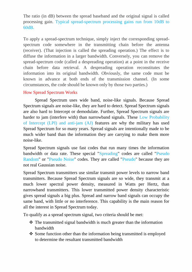
The ratio (in dB) between the spread baseband and the original signal is called

processing gain. Typical spread-spectrum processing gains run from 10dB to

60dB.

To apply a spread-spectrum technique, simply inject the corresponding spread-

spectrum code somewhere in the transmitting chain before the antenna

(receiver). (That injection is called the spreading operation.) The effect is to

diffuse the information in a larger bandwidth. Conversely, you can remove the

spread-spectrum code (called a despreading operation) at a point in the receive

chain before data retrieval. A despreading operation reconstitutes the

information into its original bandwidth. Obviously, the same code must be

known in advance at both ends of the transmission channel. (In some

circumstances, the code should be known only by those two parties.)

How Spread Spectrum Works

Spread Spectrum uses wide band, noise-like signals. Because Spread

Spectrum signals are noise-like, they are hard to detect. Spread Spectrum signals

are also hard to Intercept or demodulate. Further, Spread Spectrum signals are

harder to jam (interfere with) than narrowband signals. These Low Probability

of Intercept (LPI) and anti-jam (AJ) features are why the military has used

Spread Spectrum for so many years. Spread signals are intentionally made to be

much wider band than the information they are carrying to make them more

noise-like.

Spread Spectrum signals use fast codes that run many times the information

bandwidth or data rate. These special "Spreading" codes are called "Pseudo

Random" or "Pseudo Noise" codes. They are called "Pseudo" because they are

not real Gaussian noise.

Spread Spectrum transmitters use similar transmit power levels to narrow band

transmitters. Because Spread Spectrum signals are so wide, they transmit at a

much lower spectral power density, measured in Watts per Hertz, than

narrowband transmitters. This lower transmitted power density characteristic

gives spread signals a big plus. Spread and narrow band signals can occupy the

same band, with little or no interference. This capability is the main reason for

all the interest in Spread Spectrum today.

To qualify as a spread spectrum signal, two criteria should be met:

The transmitted signal bandwidth is much greater than the information

bandwidth

Some function other than the information being transmitted is employed

to determine the resultant transmitted bandwidth

What Spread Spectrum Does?

The use of these special pseudo noise codes in spread spectrum (SS)

communications makes signals appear wide band and noise-like. It is this very

characteristic that makes SS signals possess the quality of Low Probability of

Intercept. SS signals are hard to detect on narrow band equipment because the

signal's energy is spread over a bandwidth of maybe 100 times the information

bandwidth.

The spread of energy over a wide band, or lower spectral power density,

makes SS signals less likely to interfere with narrowband communications.

Narrow band communications, conversely, cause little to no interference to SS

systems because the correlation receiver effectively integrates over a very wide

bandwidth to recover an SS signal. The correlator then "spreads" out a narrow

band interferer over the receiver's total detection bandwidth. Since the total

integrated signal density or SNR at the correlator's input determines whether

there will be interference or not. All SS systems have a threshold or tolerance

level of interference beyond which useful communication ceases. This tolerance

or threshold is related to the SS processing gain. Processing gain is essentially

the ratio of the RF bandwidth to the information bandwidth.

A typical commercial direct sequence radio, might have a processing gain

of from 11 to 16 dB, depending on data rate. It can tolerate total jammer power

levels of from 0 to 5 dB stronger than the desired signal. Yes, the system can

work at negative SNR in the RF bandwidth. Because of the processing gain of

the receiver's correlator, the system functions at positive SNR on the baseband

data.

CHIP: The time it takes to transmit a bit or single symbol of a PN code.

CODE: A digital bit stream with noise-like characteristics.

CORRELATOR: The SS receiver component that demodulates a Spread

Spectrum signal.

DE-SPREADING: The process used by a correlator to recover

narrowband information from a spread spectrum signal.

PN: Pseudo Noise - a digital signal with noise-like properties.

Modulator

Input Data Output Data

Spreading code Spreading code

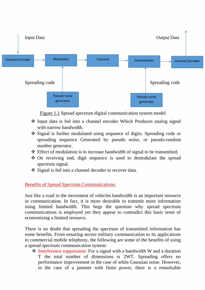
Figure 1.1 Spread spectrum digital communication system model

Input data is fed into a channel encoder Which Produces analog signal

with narrow bandwidth.

Signal is further modulated using sequence of digits. Spreading code or

spreading sequence Generated by pseudo noise, or pseudo-random

number generator.

Effect of modulation is to increase bandwidth of signal to be transmitted.

On receiving end, digit sequence is used to demodulate the spread

spectrum signal.

Signal is fed into a channel decoder to recover data.

Benefits of Spread Spectrum Communications:

Just like a road in the movement of vehicles bandwidth is an important resource

in communication. In fact, it is more desirable to transmit more information

using limited bandwidth. This begs the question why spread spectrum

communications is employed yet they appear to contradict this basic tenet of

economizing a limited resource.

There is no doubt that spreading the spectrum of transmitted information has

some benefits. From ensuring secure military communication to its applications

in commercial mobile telephony, the following are some of the benefits of using

a spread spectrum communication system:

Interference suppression: For a signal with a bandwidth W and a duration

T the total number of dimensions is 2WT. Spreading offers no

performance improvement in the case of white Gaussian noise. However,

in the case of a jammer with finite power, there is a remarkable

Channel Demodulator Channel Decoder

Pseudo noise

generator Pseudo noise

generator

Channel Encoder

improvement in the performance. The jammer may either decide to jam

all available coordinates effectively reducing the jamming intensity per

coordinate or jam a few of the probable coordinates with more power. In

either of the above options the power spectral density of the jammer

interference is effectively reduced after spreading.

Low power spectral density: This makes it possible to achieve hiding of

the signal and is the basis for low probability of intercept (LPI)

communications. It also makes it possible to conform to acceptable

regulator transmission power spectral density levels.

High resolution time of arrival measurements for precise ranging: Delay

measurements can be used to take position measurements. Theoretically,

uncertainty in delay has an inverse relationship with the bandwidth of a

transmitted pulse. As a consequence, spread spectrum communication

systems, which have a large bandwidth, provide a suitable way of

determining position location.

Multiple access: Spread spectrum techniques offer a platform for

simultaneous system access by several users in a coordinated manner

thus allowing channel sharing.

Alleviation of multipath propagation: The good performance of spread

spectrum systems in multipath channels enables them to be useful in

fading channels. Both transmit as well as receive antenna diversity is

possible with spread spectrum communication systems.

Processing Gain

An important characteristic of a spread spectrum system is the processing

gain (Gp). It is defined as the ratio of the spread bandwidth (BW) to the

bandwidth of the information (R), which can be written as follows:

Gp = Bandwidth of SpreadSignal (BW )

Bandwidth of digital information signal (R)

It‟s a measure of difference between the system performance when using

Spread Spectrum techniques & the system performance when not using Spread

Spectrum techniques.

Processing gain of Spread Spectrum is also known as Bandwidth

Expansion Factor. This is because it gives the factor, by which the bandwidth of

digital message signal is expanded.

Channel Capacity:

The basis for using a wide band system for transmission is based on

Shannon‟s limit of information capacity.

The capacity of a channel is

C=B𝑙𝑜𝑔2 1 +𝑆

𝑁

Where,

C Capacity (bits/sec)

B Bandwidth(Hz)

NNoise Power

S Signal Power

This equation means that the channel capacity is directly proportional to channel

bandwidth for a given SNR.

In Spread Spectrum it takes wide bandwidth to provide high information rates as

given by Shannon‟s limit.

Pseudo noise (PN) Sequences:

PN sequences are codes that appear to be random but are not, strictly

speaking, random since they are generated using predetermined circuit

connections. Nevertheless, they meet a number of randomness criteria.

A discussion of PN sequences is necessary in the context of synchronization

since one reason as to why PN sequences are chosen for FHSS systems are that

they have specific correlation properties that make alignment of the PN

sequences used at the transmitter and the receiver easier.

PN sequences are usually generated using Linear Feedback Shift Registers

(LFSR) based on Galois Field arithmetic. The length of the PN sequence

depends on the number of shift register stages. If there are m shift registers used,

the maximum possible PN sequence length, p is given as in below equation:

p=2n−1

Such a sequence is referred to as a maximal length sequence and they are

obtained from standard Galois Field Tables for the generation of maximal length

sequences.

As an example consider the case of a 4-stage LFSR used to generate PN

sequences. The generator polynomial that yields the maximal length sequence in

such a case is given by equation below. For other n-stage LFSRs, the generator

polynomials for maximal length sequences can be obtained from standard

generator polynomial tables.

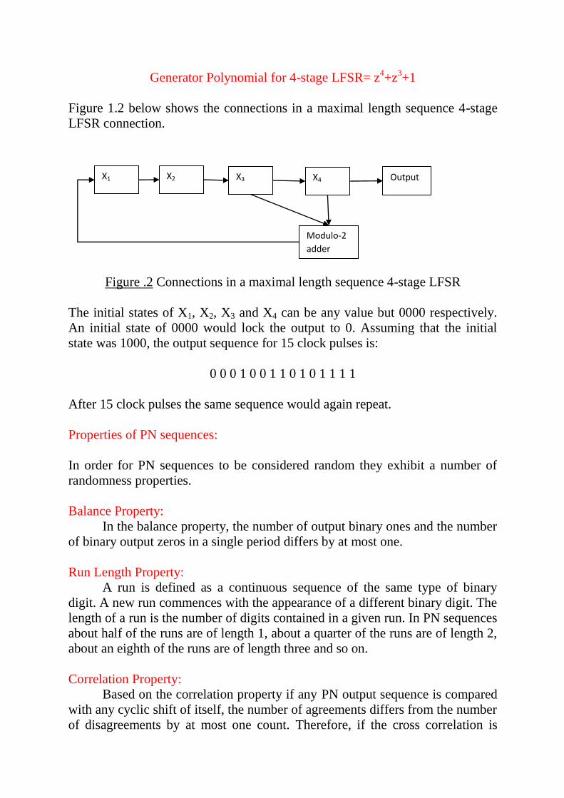
Generator Polynomial for 4-stage LFSR= z4+z

3+1

Figure 1.2 below shows the connections in a maximal length sequence 4-stage

LFSR connection.

Figure .2 Connections in a maximal length sequence 4-stage LFSR

The initial states of X1, X2, X3 and X4 can be any value but 0000 respectively.

An initial state of 0000 would lock the output to 0. Assuming that the initial

state was 1000, the output sequence for 15 clock pulses is:

0 0 0 1 0 0 1 1 0 1 0 1 1 1 1

After 15 clock pulses the same sequence would again repeat.

Properties of PN sequences:

In order for PN sequences to be considered random they exhibit a number of

randomness properties.

Balance Property:

In the balance property, the number of output binary ones and the number

of binary output zeros in a single period differs by at most one.

Run Length Property:

A run is defined as a continuous sequence of the same type of binary

digit. A new run commences with the appearance of a different binary digit. The

length of a run is the number of digits contained in a given run. In PN sequences

about half of the runs are of length 1, about a quarter of the runs are of length 2,

about an eighth of the runs are of length three and so on.

Correlation Property:

Based on the correlation property if any PN output sequence is compared

with any cyclic shift of itself, the number of agreements differs from the number

of disagreements by at most one count. Therefore, if the cross correlation is

X1 X2 X3 X4

Modulo-2

adder

Output

done for different shifts, there will be maximum correlation when there is no

shift and minimum correlation when the cyclic shift is one or more.

The correlation property makes synchronization easier since during

synchronization, by correlating the transmitter PN sequence with the receiver

PN sequence the receiver PN sequence can be continuously delayed until a set

threshold of the correlation under which acquisition can be declared is attained.

Based on the above fact it is evident that for a large stage PN sequence

the acquisition time may be larger since the maximum possible number of cyclic

shifts is also large. For shorter PN sequence lengths, the acquisition time lasts

shorter time durations. However, the length of the PN sequence that is used is

not the only factor that determines the acquisition time. The nature of the

communication channel also plays a part in determining the acquisition time.

Classifications of Spread Spectrum Systems:

There are two major classes of spread spectrum systems. These are:

Pure spread spectrum systems

Hybrid spread spectrum systems

Under pure spread spectrum systems, the following three spread spectrum

systems are obtained:

Direct Sequence Spread Spectrum (DSSS)

Frequency Hopping Spread Spectrum (FHSS)

Time Hopping Spread Spectrum (THSS)

Hybrid systems are obtained by combining two or more of the pure spread

spectrum systems. The primary goal of hybrid systems is to tap into and exploit

the unique advantages of each of the pure spread spectrum systems used.

While doing this, hybrid systems combat each of the individual shortcomings of

each of the spread spectrum systems.

Consider a hybrid Direct Sequence- Frequency Hopping Spread Spectrum

(DS/FH) system. When employed in a channel with interference in specific

bands, a frequency hopping algorithm can be employed to effect hops only into

suitable bands. After hopping into the desirable bands, a direct sequence spread

can be effected. This improves the spreading gain of the hybrid system and as a

result improves the system performance in channels where most of the noise

occurs in few frequency bands which can be predicted.

The main hybrid spread spectrum systems are as follows:

DS/FH

DS/TH

FH/TH

DS/FH/TH

As earlier mentioned, spread spectrum systems use pseudo random signals to

effect the spreading. These spreading sequences are referred to as pseudo noise

(PN) sequences or PN codes. For the purposes of the project, PN sequences will

be generated using linear feedback shift registers. PN sequences have a number

of properties that make them reliable as compared to other codes during

acquisition.

Direct Sequence Spread Spectrum Systems:

In DSSS spreading is achieved by representing each bit of the original

message sequence using several bits. This process is achieved by using a

spreading code in this case a PN sequence.

The PN sequence is XOR-ed with the message sequence. As a case in point,

consider a case where the PN sequences are produced at a frequency that is 10

times higher than the message frequency. In this case, the message frequency

will be spread by a factor of 10 after the XOR process. This step details the

transmission process in a DSSS system.

At the receiver, the transmitted signal is again XOR-ed using a PN sequence

that is similar to the one originally used at the transmitter. In this way the

original message sequence can be recovered.

However, channel imperfections bring in the need for synchronization of the

spreading sequence used at the transmitter, and the one employed at the

receiver. This makes the code synchronization steps of code acquisition and

code tracking important. These steps are also important in FHSS systems

In code acquisition, the PN sequence employed at the transmitter and the one

employed at the receiver are brought to within one-time period of the original

spreading sequence. In code tracking, the PN sequence at the receiver that has

already been brought to within one-time period of that used at the transmitter by

code acquisition is further refined and its accuracy is brought to within less than

half of the time period of the code employed at the transmitter.

In practice code acquisition takes place before code tracking after which code

tracking is initiated. The basis for code acquisition is correlating both the PN

sequences used at the transmitter and the receiver and setting a threshold which

once attained, acquisition is declared to have occurred. PN sequences are the

most effective spreading sequences since as will be highlighted later they have

maximum correlation when both PN sequences are in sync and minimum

correlation which remains constant when the signals are out of sync.

The code acquisition process takes place over a finite amount of time. When

longer PN sequences are used the acquisition time may be longer. In order to

appreciate this fact, a brief description of what acquisition involves is necessary.

During acquisition, the PN sequence received from the receiver is compared

with the one that is to be employed at the transmitter. If the correlation is below

a set threshold, the PN sequence at the receiver is delayed by a single time

period of the PN sequence. This process goes on and on recursively until a set

threshold is attained. Once this threshold is attained acquisition is said to have

occurred.

If PN sequence has 15 output sequence orders while another one has 7 output

sequence orders, the maximum amount of acquisition for the 15 sequence PN

sequence will be 15 time durations on the one hand. On the other hand, for the 7

sequence PN sequence, the maximum acquisition time will be 7 time periods.

This shows the effect of the length of the PN sequence on acquisition time.

However, this is the worst case scenario and typical acquisition times may

actually last a shorter time period. However, making use of a longer spreading

sequence increases the spreading gain but in light of the fact that a longer

spreading sequence increases the acquisition time, a trade off definitely exists.

The choice is between having a greater spreading gain and longer acquisition

times and vice versa.

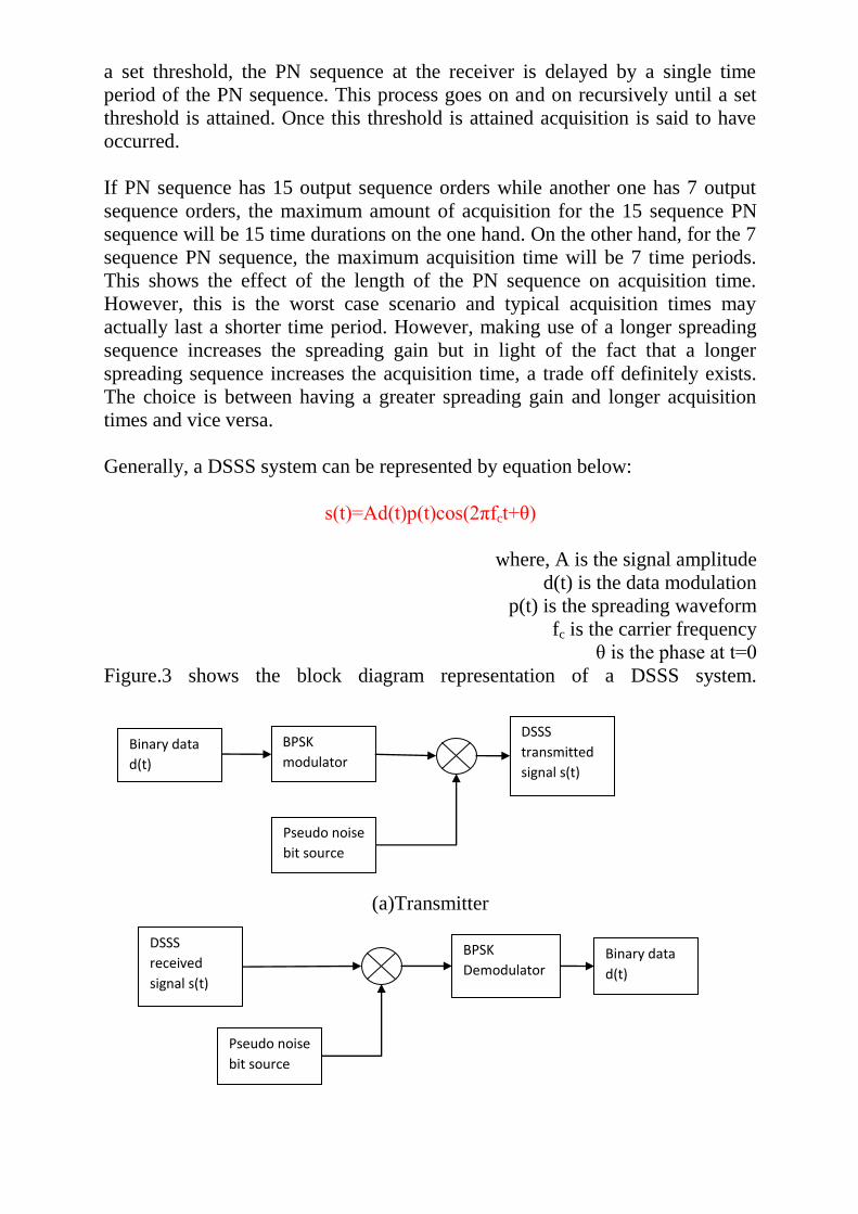
Generally, a DSSS system can be represented by equation below:

s(t)=Ad(t)p(t)cos(2πfct+θ)

where, A is the signal amplitude

d(t) is the data modulation

p(t) is the spreading waveform

fc is the carrier frequency

θ is the phase at t=0

Figure.3 shows the block diagram representation of a DSSS system.

(a)Transmitter

BPSK

modulator

Binary data

d(t)

Pseudo noise

bit source

DSSS

transmitted

signal s(t)

DSSS

received

signal s(t)

Pseudo noise

bit source

BPSK

Demodulator

Binary data

d(t)

(b) Receiver

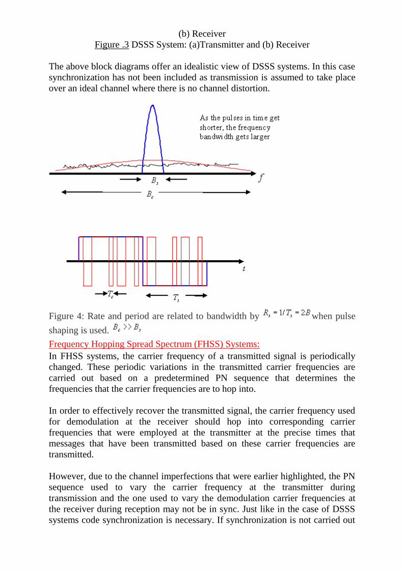
Figure .3 DSSS System: (a)Transmitter and (b) Receiver

The above block diagrams offer an idealistic view of DSSS systems. In this case

synchronization has not been included as transmission is assumed to take place

over an ideal channel where there is no channel distortion.

Figure 4: Rate and period are related to bandwidth by when pulse

shaping is used.

Frequency Hopping Spread Spectrum (FHSS) Systems:

In FHSS systems, the carrier frequency of a transmitted signal is periodically

changed. These periodic variations in the transmitted carrier frequencies are

carried out based on a predetermined PN sequence that determines the

frequencies that the carrier frequencies are to hop into.

In order to effectively recover the transmitted signal, the carrier frequency used

for demodulation at the receiver should hop into corresponding carrier

frequencies that were employed at the transmitter at the precise times that

messages that have been transmitted based on these carrier frequencies are

transmitted.

However, due to the channel imperfections that were earlier highlighted, the PN

sequence used to vary the carrier frequency at the transmitter during

transmission and the one used to vary the demodulation carrier frequencies at

the receiver during reception may not be in sync. Just like in the case of DSSS

systems code synchronization is necessary. If synchronization is not carried out

the transmitted signal will be wrongly demodulated yielding an incorrect signal

at the receiver.

In FHSS, code synchronization involves two steps namely: code acquisition and

code tracking. Just like the situation in DSSS the code acquisition phase

involves bringing the PN sequence to at least within a time period of the PN

sequence used to generate the carrier frequency at the receiver. Code tracking

involves further refining the acquired PN sequence improving its accuracy to

less than half the time period of the transmitted signal.

Spreading and Despreading

The rapid phase transition (chip rate ) signal has a larger bandwidth given that

the rate is greater (without changing the power of the original signal) and

behaves similar to noise in such a way that their spectrums are similar for

bandwidth in scope. In fact, the power density amplitude of the spread spectrum

output signal is similar to the noise floor. The signal is “hidden” under the noise.

To get the signal back, the exact same high bandwidth signal is needed. This is

like a key, only the demodulator that “knows” such a key will be able to

demodulate and get the message back. This “key” is in fact a pseudo random

sequence (rapid phase transition) also known as pseudo noise (PN). These

sequences are generated by m-sequences.

m-Sequences

These codes (DSSS codes) will all be treated as pseudo noise (PN) sequences

because resembles random sequences of bits with a flat noise like spectrum.

This sequence appears to have random pattern but in fact can be recreated by

using the shift register structure in Figure 4 with M=4,

polynomial and initial state „1 1 0 0‟.

Figure 5: Shift register structure for m-sequence

Where „ ‟ represent modulo 2 addition.

Using this scheme, the initial state is only needed to generate exactly the same

sequence of length (the only forbidden state is all zeros since the register

will lock in this state).

Take for example:

The final sequence will look like this,

1 1 -1 -1 -1 1 -1 -1 1 1 -1 1 -1 1 1

After the fifteenth shift, the values on the registers will be again the starting

seed.

Properties of m-Sequences

Period:

After this number of „1‟ and „-1‟ the sequence will start to repeat since the

starting symbols will be the same.

Autocorrelation:

The formal definition of discrete autocorrelation is:

Consider the previous sequence

1 1 -1 -1 -1 1 -1 -1 1 1 -1 1 -1 1 1

If we perform the following operation:

= 15 which is multiply each value by itself and add them all ( ).

Now take ,

Performing the same operation:

= -1 =

This is the autocorrelation for each shift point. If we take them all and plot them

so that there are 15 points before 0 and 15 after:

a)

b)

Figure 6: Correlation of a) example sequence and b) other sequence with

polynomial created with LabVIEW and MathScript

As seen, only if the end user having the exact sequence is able to demodulate

the message when the sequence is synchronized (peak at correlation = 1). Other

users will have very little amplitude of the original signal. This is the principle

of Code Division Multiple Access (CDMA) cellular systems, in other words,

share the same frequency and time with multiple users with different codes.

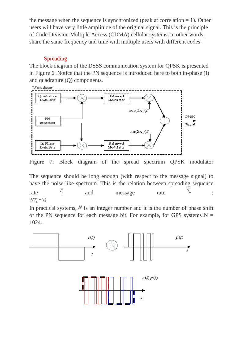
Spreading

The block diagram of the DSSS communication system for QPSK is presented

in Figure 6. Notice that the PN sequence is introduced here to both in-phase (I)

and quadrature (Q) components.

Figure 7: Block diagram of the spread spectrum QPSK modulator

The sequence should be long enough (with respect to the message signal) to

have the noise-like spectrum. This is the relation between spreading sequence

rate and message rate :

In practical systems, is an integer number and it is the number of phase shift

of the PN sequence for each message bit. For example, for GPS systems N =

1024.

Figure 8: Spreading the message, each bit of the message will contain

the entire PN sequence

The new message has now and therefore

The output combined baseband sequence is:

Where is the sent baseband waveform, is the PN waveform and is

the bit sequence.

Despreading

Received baseband waveform is the combination of the transmitted waveform

and noise in the channel.

Figure 9: Simple additive white Gaussian noise (AWDG) channel model.

The received signal will be combined again with the spreading sequence. Notice

that the noise is also going to be processed on the same procedure but

correlation properties will not increase the noise power.

The received signal will be the combination of the transmitted signal plus

noise:

We can substitute the sent waveform by the combination of the PN sequence

and the bit sequence.

The modulator will multiply it by the PN sequence :

If is synchronized, and is like multiplying noise times

noise which gives other kind of noise (similar in amplitude).

Consider the ideal example from Figure 10.

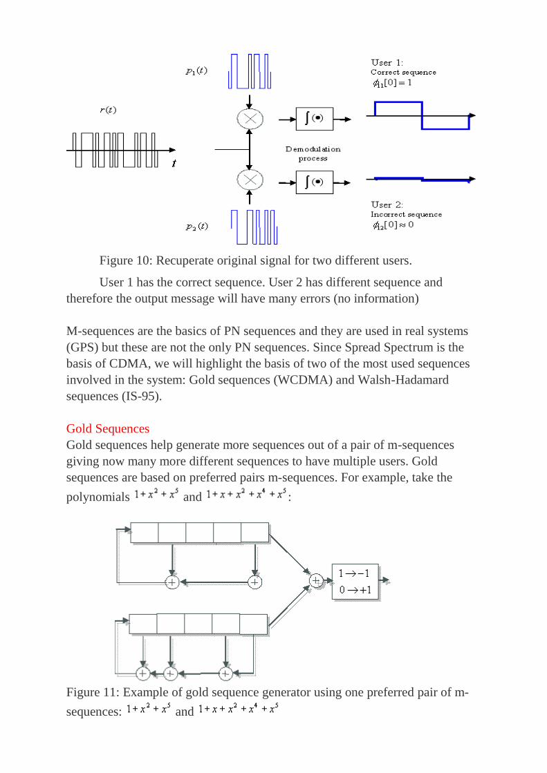
Figure 10: Recuperate original signal for two different users.

User 1 has the correct sequence. User 2 has different sequence and

therefore the output message will have many errors (no information)

M-sequences are the basics of PN sequences and they are used in real systems

(GPS) but these are not the only PN sequences. Since Spread Spectrum is the

basis of CDMA, we will highlight the basis of two of the most used sequences

involved in the system: Gold sequences (WCDMA) and Walsh-Hadamard

sequences (IS-95).

Gold Sequences

Gold sequences help generate more sequences out of a pair of m-sequences

giving now many more different sequences to have multiple users. Gold

sequences are based on preferred pairs m-sequences. For example, take the

polynomials and :

Figure 11: Example of gold sequence generator using one preferred pair of m-

sequences: and

Remember m-sequences gave only one sequence of length . By combining

two of these sequences, we can obtain up to 31 ( ) plus the two m-sequences

themselves, generate 33 sequences (each one length ) that can be used to

spread different input messages (different users CDMA).

The m-sequence pair plus the Gold sequences form the available

sequences to use in DSSS. The wanted property about Gold codes is that they

are balanced (i.e. same number of 1 and -1s).

Walsh-Hadamard Sequences

Other common sequences are Walsh-Hadamard sequences currently used in

CDMA systems. These sequences are orthogonal (i.e. where is a

row of the matrix), convenient properties for multiple users. The sequences are

the rows of the Hadamard matrix defined for as:

For larger matrices use the recursion:

Example for

Orthogonal codes have perfect properties of cross correlation (if no shift is

implemented).

Positive Performance features of SS technique

These are the techniques which help in the digital communication

scenario.

The techniques are

Interference Rejection

Energy Density Reduction

High Resolution Ranging

Multiple Access

Interference Rejection

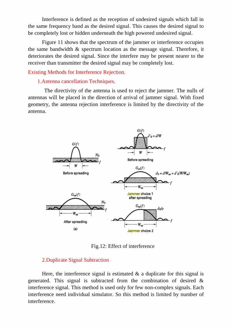
Interference is defined as the reception of undesired signals which fall in

the same frequency band as the desired signal. This causes the desired signal to

be completely lost or hidden underneath the high powered undesired signal.

Figure 11 shows that the spectrum of the jammer or interference occupies

the same bandwidth & spectrum location as the message signal. Therefore, it

deteriorates the desired signal. Since the interfere may be present nearer to the

receiver than transmitter the desired signal may be completely lost.

Existing Methods for Interference Rejection.

1.Antenna cancellation Techniques.

The directivity of the antenna is used to reject the jammer. The nulls of

antennas will be placed in the direction of arrival of jammer signal. With fixed

geometry, the antenna rejection interference is limited by the directivity of the

antenna.

Fig.12: Effect of interference

2.Duplicate Signal Subtraction

Here, the interference signal is estimated & a duplicate for this signal is

generated. This signal is subtracted from the combination of desired &

interference signal. This method is used only for few non-complex signals. Each

interference need individual simulator. So this method is limited by number of

interference.

3. Selective Rejecters

Selective Rejecters such as Notch filters are used for interference

rejection. This method is effective when used for narrowband interferers. In case

of wideband interferers, some of the desired signal may be rejected along with

interference signal.

Spread Spectrum Interference Rejection model

The following figure shows the basic principle in the interference cababilities of

SS technique.

m(t)s(t)+n(t)

m(t)

m(t)s(t)

s(t)

Fig.13: Model for SS Transmitter

m(t)s(t)+n(t)

From Channel

m(t)s2(t)

+n(t)s(t)

m(t)

s(t)

Spread Spectrum Code

Signal

Data Generator

Spread Spectrum Code

Signal

Band Pass Filter

Fig.14: Model for SS Receiver

Let

m(t)Message signal with data rate R bits/sec

s(t) SS Spreading code signal with chip rate

R Transmission bandwidth of message signal

Rss Transmission bandwidth of Spreading code signal

m(t)s(t) M(w)*S(w)

The Bandwidth of data signal is narrow compared to spreading code.

Bandwidth of SS or product signal is approximately equal to bandwidth of

spreading code.

Energy Density Reduction

Energy Density Reduction offers the following advantages.

1. Low probability of detection

2. High power levels for the message signal for satellite communication

Radiometer is used to decide whether the transmitted signal is present or not.

Fig.15: block diagram of radiometer

The receiver antenna scans the channel for transmitted signal. The received

signal is passed through the BPF, which is cantered at central frequency of

transmitted signal.

The signal is passed to squarer & it gives it output to integrator which integrates

that output(energy). This energy is sampled by the switch, which gives the value

accumulated in the integrator during a period.

Now comparator gets 2 inputs, one from switch & another form threshold

generator which gives threshold values. By comparing these 2 values,

comparator gives the decision like whether the transmitted signal in present or

not.

The bandwidth of spread spectrum signal is high & having low power level than

message signal. Therefore, the application of SS also reduces the probability

that the signal is perceived to be present by such radiometers.

SS offers low probability detection by using its property of energy density

function.

High resolution Ranging:

In RADAR, the time delay between the transmitter & the reception of pulse

provides the distance of location of the target. One of the disadvantages of using

single pulse for this purpose is that one shot pulse is not reliable over a Gaussian

channel. This can be avoided by using SS techniques

1. Due to correlation properties of SS, the SS signal can be accurately

detected even when it is buried deep in noise. This will increase the target

detection in RADAR applications

2. Due to high bandwidths used in SS, the time resolution of pulse will be

less. Therefore, the distance of location of target can be found precisely

with better resolution.

Multiple Access:

SS techniques also provides multiple access & are different from other

techniques.

For example, in TDMA, the time is sliced between different users, where each

user can use the entire bandwidth during that time slice.

In FDMA, each user is allocated a narrow bandwidth channel with low data

rates, but continuous transmission all the time.

In SS all the users use the entire Bandwidth all the time. So high data rates &

high speed of data transmission is possible due to availability of continuous

transmission. But there are some possibilities for huge interference due to

overlap in both time & channel bandwidths.

This can be avoided by using high different spreading code for different users.

The high autocorrelation property of spreading code helps receive the desired

signal.

Limitations of Spread Spectrum:

1. No performance improvement in AWGN channels

2. Complex Implementation

3. Bandwidth Inefficiency:

The bandwidth used for SS communication is very high compared to

bandwidth of data signal. But the bandwidth is not efficiently used in SS.

The initial concentration of SS has been on ant jam & interference

rejection.

Jamming Methods:

Jammer:

An intentional or unintentional coherent, unwanted disturbances

to the desired signal, usually in the same frequency band of desired signal.

Jamming:

Electromagnetic jamming is defined as the deliberate radiation, re-

radiation or reflection of electromagnetic energy to prevent or reduce the

enemy‟s effective use of electromagnetic spectrum. Also used to degrade or

neutralize the enemy‟s combat compatibility.

The goal of jammer is to disturb the communication. The goals of

communicator are to develop a jam-resistant communication system under the

following assumptions.

1. Compute invulnerability is not possible

2. The jammer has a prior knowledge of most system parameters,

frequency bands, timings, traffic……

3. The jammer has no prior knowledge of PN spreading code.

Protection against jamming waveforms is provided purposely making the

information-beating signal occupy a Bandwidth far in excess of minimum

Bandwidth necessary to transmit it. This has the effect of making the transmitted

signal assume noise like appearance. So as to blend into background. Thus the

signal is enabled to propagate through the channel.

Jamming Types:

Based on communication channels where jamming occurs,the

jamming is classified as follows.

Radio Jamming

RADAR Jamming

Pulse Noise Jamming in coherent BPSK System

Radio Jamming

Radio jamming is the intentional jamming caused near the central

frequency of receiver. So receiver receives unwanted signal rather than actual

message signal. This is achieved by high power jammer signal. Since message

signal having less power, it is lost as noise & receiver receives only the jammer

signal.

Two types of Radio Jamming are there

1.Obvious Jamming

2.Subtle jamming

1.Obvious Jamming

Here the receiver can immediately detect the presence of a

jammer.

It sends out noise tone like stepped tones & random keying

codes in the frequency range of operation of the receiver.

The receiver can hear those sounds on its devices. This

overrides the message signal. Since this type of noise is

detected, the receiver can take action to avoid effects of the

jammer.

It may jump to another frequency band of operation to

avoid the jammer effects.

2.Subtle Jamming

This type of jamming remains undetected at the receiver.

The receiver has no knowledge that the information-bearing

signal is lost.

The receiver doesn‟t recognize the problem & continue

with its normal operation.

This type of jamming is very dangerous as it is very

difficult to detect & resist.

RADAR Jamming

RADAR Jamming is the transmission of signals in the frequency

band of operation of RADAR with the intention of either blocking the

information or manipulating the information.

Two types of RADAR jamming are there.

1.Noise Jammers

2.Deception Jammers

1.Noise Jammers

The purpose of this jammer is to either delay the detection

of target or to avoid it.

This is achieved by transmitting a high powered signal

within the frequency band of operation of RADAR.

This appears as thermal noise received by RADAR & the

target goes undetected.

2.Deception Jammers

The purpose of this jammer is to send out false information

regarding the location, direction of travel & velocity of

target to the RADAR.

This can be done by intercepting the original RADAR

signal. They modify the information & retransmit the false

information to the RADAR receiver.

Pulse Noise Jamming in Coherent BPSK System

Pulse Noise jammer transmits pulse of band limited white

Gaussian noise with the total average power of J. The effect of jammer is more

if it is successful in modelling its central frequency & bandwidth to be identical

with the communication channel.

The probability of bit error is given by

PB=Q((2Eb/N0)1/2

)

Where,

Eb

Energy per bit

N0

Receiver front end thermal noise

While transmitting the noise pulse within the receiver bandwidth, the noise

spectral density increases.

New thermal noise is N0‟ = N0 + NJ/ρ

Where,

NJ Jammer power spectral density

ρ duty factor

Now the new increased average probability of error is

P B‟= (1- ρ) Q((2Eb/N0)1/2

) + ρQ ((2Eb/ N0‟)1/2

)

Compared to noise introduced by jammer, the thermal noise of RADAR, the

first term in above equation is negligible.

So

P B‟= ρQ ((2Ebρ/ N0‟)1/2

)