SECTION THREE Introduction to Descriptive Statistics and ... · Statistics and Discrete Probability...
172
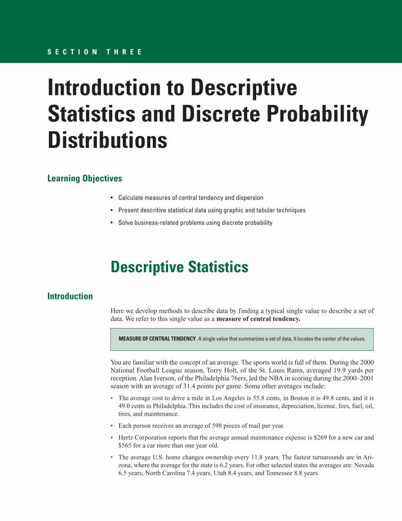
SECTION THREE Introduction to Descriptive Statistics and Discrete Probability Distributions Learning Objectives • Calculate measures of central tendency and dispersion • Present descritive statistical data using graphic and tabular techniques • Solve business-related problems using discrete probability Descriptive Statistics Introduction Here we develop methods to describe data by finding a typical single value to describe a set of data. We refer to this single value as a measure of central tendency. You are familiar with the concept of an average. The sports world is full of them. During the 2000 National Football League season, Torry Holt, of the St. Louis Rams, averaged 19.9 yards per reception. Alan Iverson, of the Philadelphia 76ers, led the NBA in scoring during the 2000–2001 season with an average of 31.4 points per game. Some other averages include: • The average cost to drive a mile in Los Angeles is 55.8 cents, in Boston it is 49.8 cents, and it is 49.0 cents in Philadelphia. This includes the cost of insurance, depreciation, license, fees, fuel, oil, tires, and maintenance. • Each person receives an average of 598 pieces of mail per year. • Hertz Corporation reports that the average annual maintenance expense is $269 for a new car and $565 for a car more than one year old. • The average U.S. home changes ownership every 11.8 years. The fastest turnarounds are in Ari- zona, where the average for the state is 6.2 years. For other selected states the averages are: Nevada 6.5 years, North Carolina 7.4 years, Utah 8.4 years, and Tennessee 8.8 years. MEASURE OF CENTRAL TENDENCY A single value that summarizes a set of data. It locates the center of the values.
-
Upload
vuongthien -
Category
Documents
-
view
225 -
download
0
Transcript of SECTION THREE Introduction to Descriptive Statistics and ... · Statistics and Discrete Probability...
S E C T I O N T H R E E
Introduction to DescriptiveStatistics and Discrete ProbabilityDistributionsLearning Objectives
• Calculate measures of central tendency and dispersion
• Present descritive statistical data using graphic and tabular techniques
• Solve business-related problems using discrete probability
Descriptive Statistics
IntroductionHere we develop methods to describe data by finding a typical single value to describe a set ofdata. We refer to this single value as a measure of central tendency.
You are familiar with the concept of an average. The sports world is full of them. During the 2000National Football League season, Torry Holt, of the St. Louis Rams, averaged 19.9 yards perreception. Alan Iverson, of the Philadelphia 76ers, led the NBA in scoring during the 2000–2001season with an average of 31.4 points per game. Some other averages include:
• The average cost to drive a mile in Los Angeles is 55.8 cents, in Boston it is 49.8 cents, and it is49.0 cents in Philadelphia. This includes the cost of insurance, depreciation, license, fees, fuel, oil,tires, and maintenance.
• Each person receives an average of 598 pieces of mail per year.
• Hertz Corporation reports that the average annual maintenance expense is $269 for a new car and$565 for a car more than one year old.
• The average U.S. home changes ownership every 11.8 years. The fastest turnarounds are in Ari-zona, where the average for the state is 6.2 years. For other selected states the averages are: Nevada6.5 years, North Carolina 7.4 years, Utah 8.4 years, and Tennessee 8.8 years.
MEASURE OF CENTRAL TENDENCY A single value that summarizes a set of data. It locates the center of the values.

There is not just one measure of central tendency; in fact, there are many. We will considerfive: the arithmetic mean, the weighted mean, the median, the mode, and the geometric mean. Wewill begin by discussing the most widely used and widely reported measure of central tendency,the arithmetic mean.
The Population MeanMany studies involve all the values in a population. If we report that the mean ACT score of allstudents entering the University of Toledo in the Fall of 2000 is 19.6, this is an example of a pop-ulation mean because we have a score for all students who entered in the fall of 2000. There are12 sales associates employed at the Reynolds Road outlet of Carpets by Otto. The mean amountof commission they earned last month was $1,345. We consider this a population value becausewe considered all the sales associates. Other examples of a population mean would be: the meanclosing price for Johnson and Johnson stock for the last five days is $98.75; the mean annual rateof return for the last 10 years for Berger Funds is 8.67 percent; and the mean number of hours ofovertime worked last week by the six welders in the welding department of the Struthers WellsCorp. is 6.45 hours.
For raw data, that is, data that has not been grouped in a frequency distribution or a stem-and-leaf display, the population mean is the sum of all the values in the population divided by thenumber of values in the population. To find the population mean, we use the following formula.
Population mean �
Instead of writing out in words the full directions for computing the population mean (or anyother measure), it is more convenient to use the shorthand symbols of mathematics. The mean ofa population using mathematical symbols is:
POPULATION MEAN � � [3–1]
where:
� represents the population mean. It is the Greek lowercase letter “mu.”
N is the number of items in the population.
X represents any particular value.
� is the Greek capital letter “sigma” and indicates the operation of adding.
�� is the sum of the X values.Any measurable characteristic of a population is called a parameter. The mean of a popula-
tion is a parameter.
Snapshot 3–1Did you ever meet the “average” American man? Well, his name is Robert (that is the nominal level of measurement), he is 31 years old (that is theratio level), he is 69.5 inches tall (again the ratio level of measurement), weighs 172 pounds, wears a size 91⁄2 shoe, has a 34-inch waist, and wears asize 40 suit. In addition, the average man eats 4 pounds of potato chips, watches 2,567 hours of TV, receives 598 pieces of mail, and eats 26 poundsof bananas each year. Also, he sleeps 7.7 hours per night. Is this really an “average” man or would it be better to refer to him as a “typical” man?Would you expect to find a man with all these characteristics?
�XN
Sum of all the values in the populationNumber of values in the population
270 Section Three
Example
Solution
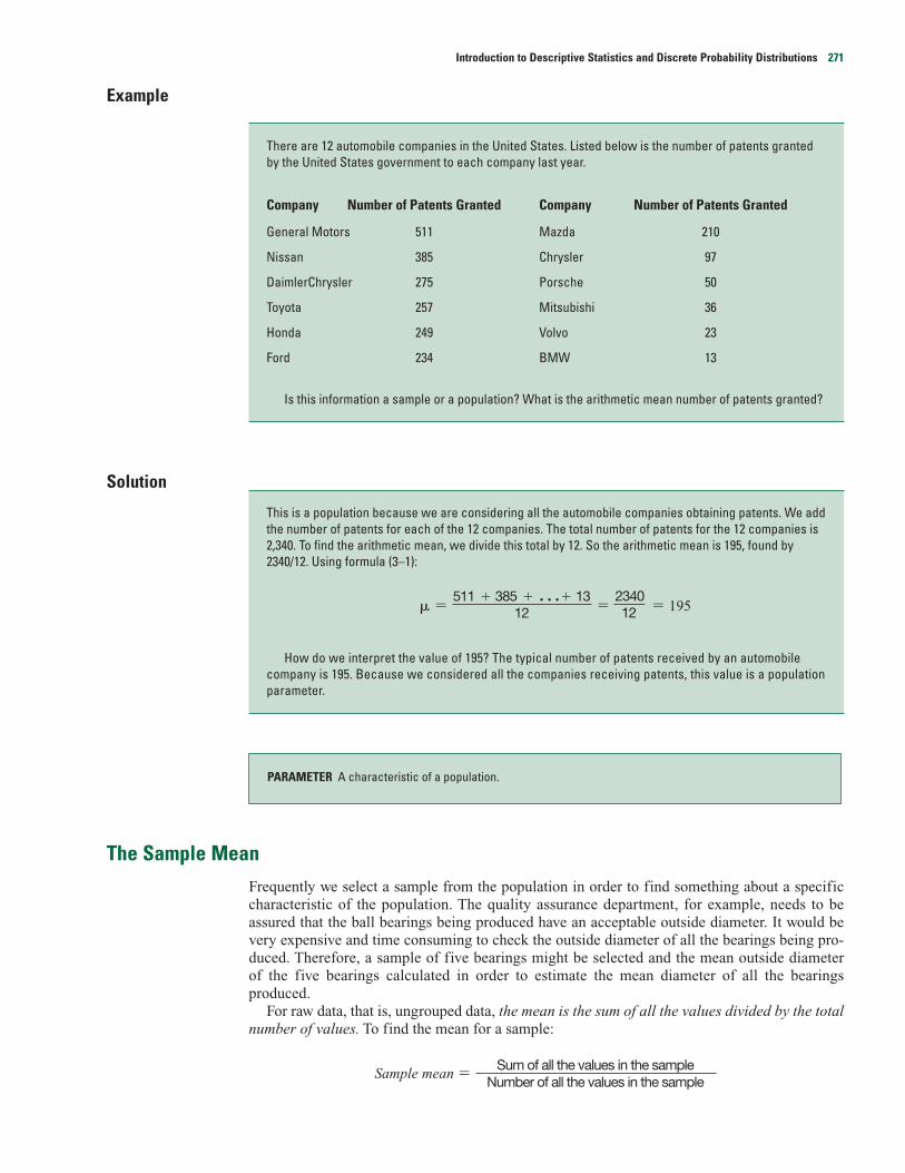
This is a population because we are considering all the automobile companies obtaining patents. We addthe number of patents for each of the 12 companies. The total number of patents for the 12 companies is2,340. To find the arithmetic mean, we divide this total by 12. So the arithmetic mean is 195, found by2340/12. Using formula (3–1):
� � � � 195
How do we interpret the value of 195? The typical number of patents received by an automobilecompany is 195. Because we considered all the companies receiving patents, this value is a populationparameter.
The Sample MeanFrequently we select a sample from the population in order to find something about a specificcharacteristic of the population. The quality assurance department, for example, needs to beassured that the ball bearings being produced have an acceptable outside diameter. It would bevery expensive and time consuming to check the outside diameter of all the bearings being pro-duced. Therefore, a sample of five bearings might be selected and the mean outside diameterof the five bearings calculated in order to estimate the mean diameter of all the bearingsproduced.
For raw data, that is, ungrouped data, the mean is the sum of all the values divided by the totalnumber of values. To find the mean for a sample:
Sample mean �Sum of all the values in the sample
Number of all the values in the sample
PARAMETER A characteristic of a population.
234012
511 � 385 � · · ·� 1312
There are 12 automobile companies in the United States. Listed below is the number of patents grantedby the United States government to each company last year.
Company Number of Patents Granted Company Number of Patents Granted
General Motors 511 Mazda 210
Nissan 385 Chrysler 97
DaimlerChrysler 275 Porsche 50
Toyota 257 Mitsubishi 36
Honda 249 Volvo 23
Ford 234 BMW 13
Is this information a sample or a population? What is the arithmetic mean number of patents granted?
Introduction to Descriptive Statistics and Discrete Probability Distributions 271
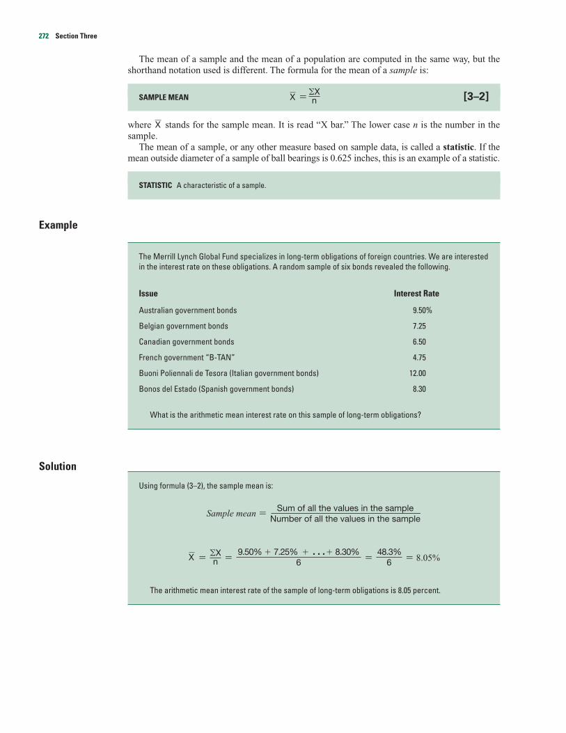
The mean of a sample and the mean of a population are computed in the same way, but theshorthand notation used is different. The formula for the mean of a sample is:
SAMPLE MEAN � [3–2]
where stands for the sample mean. It is read “X bar.” The lower case n is the number in thesample.
The mean of a sample, or any other measure based on sample data, is called a statistic. If themean outside diameter of a sample of ball bearings is 0.625 inches, this is an example of a statistic.
STATISTIC A characteristic of a sample.
Example
Solution
Using formula (3–2), the sample mean is:
Sample mean �
� � � � 8.05%
The arithmetic mean interest rate of the sample of long-term obligations is 8.05 percent.
48.3%6
9.50% � 7.25% � · · ·� 8.30%6
�XnX
Sum of all the values in the sampleNumber of all the values in the sample
The Merrill Lynch Global Fund specializes in long-term obligations of foreign countries. We are interestedin the interest rate on these obligations. A random sample of six bonds revealed the following.
Issue Interest Rate
Australian government bonds 9.50%
Belgian government bonds 7.25
Canadian government bonds 6.50
French government “B-TAN” 4.75
Buoni Poliennali de Tesora (Italian government bonds) 12.00
Bonos del Estado (Spanish government bonds) 8.30
What is the arithmetic mean interest rate on this sample of long-term obligations?
X
�XnX
272 Section Three
The Properties of the Arithmetic MeanThe arithmetic mean is a widely used measure of central tendency. It has several importantproperties:
1. Every set of interval-level data has a mean. (Recall that interval-level data include such data asages, incomes, and weights, with the distance between numbers being constant.)
2. All the values are included in computing the mean.
3. A set of data has only one mean. The mean is unique. (Later we will discover an average that mightappear twice, or more than twice, in a set of data.)
4. The mean is a useful measure for comparing two or more populations. It can, for example, be usedto compare the performance of the production employees on the first shift at the Chrysler trans-mission plant with the performance of those on the second shift.
5. The arithmetic mean is the only measure of central tendency where the sum of the deviations ofeach value from the mean will always be zero. Expressed symbolically:
�( X � ) � 0
As an example, the mean of 3, 8, and 4 is 5. Then:
�(X � ) � (3 � 5) � (8 � 5) � (4 � 5)
� �2 � 3 �1
� 0
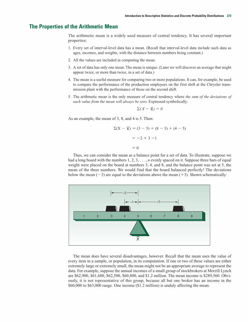
Thus, we can consider the mean as a balance point for a set of data. To illustrate, suppose wehad a long board with the numbers 1, 2, 3, . . . , n evenly spaced on it. Suppose three bars of equalweight were placed on the board at numbers 3, 4, and 8, and the balance point was set at 5, themean of the three numbers. We would find that the board balanced perfectly! The deviationsbelow the mean (�3) are equal to the deviations above the mean (�3). Shown schematically:
The mean does have several disadvantages, however. Recall that the mean uses the value ofevery item in a sample, or population, in its computation. If one or two of these values are eitherextremely large or extremely small, the mean might not be an appropriate average to represent thedata. For example, suppose the annual incomes of a small group of stockbrokers at Merrill Lynchare $62,900, $61,600, $62,500, $60,800, and $1.2 million. The mean income is $289,560. Obvi-ously, it is not representative of this group, because all but one broker has an income in the$60,000 to $63,000 range. One income ($1.2 million) is unduly affecting the mean.
–1
–2
+3
1 2 3 4 5 6 7 8 9
X
X
Introduction to Descriptive Statistics and Discrete Probability Distributions 273
The mean is also inappropriate if there is an open-ended class for data tallied into a frequencydistribution. If a frequency distribution has the open-ended class “$100,000 and more,” and thereare 10 persons in that class, we really do not know whether their incomes are close to $100,000,$500,000, or $16 million. Since we lack information about their incomes, the arithmetic meanincome for this distribution cannot be determined.
Self-Review 3–1
Exercises
1. Compute the mean of the following population values: 6, 3, 5, 7, 6.
2. Compute the mean of the following population values: 7, 5, 7, 3, 7, 4.
3. a. Compute the mean of the following sample values: 5, 9, 4, 10.
b. Show that �(X � ) � 0.
4. a. Compute the mean of the following sample values: 1.3, 7.0, 3.6, 4.1, 5.0.
b. Show that �(X � ) � 0.
5. Compute the mean of the following sample values: 16.25, 12.91, 14.58.
6. Compute the mean hourly wage paid to carpenters who earned the following wages: $15.40,$20.10, $18.75, $22.76, $30.67, $18.00.
For questions 7–10, (a) compute the arithmetic mean and (b) indicate whether it is a statisticor a parameter.
7. There are 10 salespeople employed by Midtown Ford. The numbers of new cars sold last month bythe respective salespeople were: 15, 23, 4, 19, 18, 10, 10, 8, 28, 19.
8. The accounting department at a mail-order company counted the following numbers of incomingcalls per day to the company’s toll-free number during the first seven days in May 2001: 14, 24, 19,31, 36, 26, 17.
9. The Cambridge Power and Light Company selected 20 residential customers at random. Followingare the amounts to the nearest dollar, the customers were charged for electrical service last month:
54 48 58 50 25 47 75 46 60 70
67 68 39 35 56 66 33 62 65 67
X
X
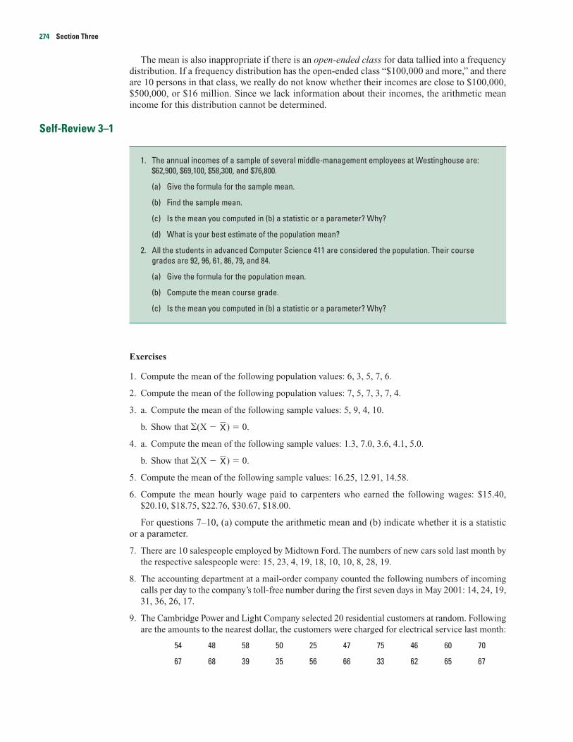
1. The annual incomes of a sample of several middle-management employees at Westinghouse are:$62,900, $69,100, $58,300, and $76,800.
(a) Give the formula for the sample mean.
(b) Find the sample mean.
(c) Is the mean you computed in (b) a statistic or a parameter? Why?
(d) What is your best estimate of the population mean?
2. All the students in advanced Computer Science 411 are considered the population. Their coursegrades are 92, 96, 61, 86, 79, and 84.
(a) Give the formula for the population mean.
(b) Compute the mean course grade.
(c) Is the mean you computed in (b) a statistic or a parameter? Why?
274 Section Three

10. The personnel director of Mercy Hospital began a study of the overtime hours of the registerednurses. Fifteen RNs were selected at random, and these overtime hours during June were noted:
13 13 12 15 7 15 5 12
6 7 12 10 9 13 12
The Weighted MeanThe weighted mean is a special case of the arithmetic mean. It occurs when there are severalobservations of the same value which might occur if the data have been grouped into a frequencydistribution. To explain, suppose the nearby Wendy’s Restaurant sold medium, large, and Biggie-sized soft drinks for $.90, $1.25, and $1.50, respectively. Of the last ten drinks sold, 3 weremedium, 4 were large, and 3 were Biggie-sized. To find the mean amount of the last ten drinkssold, we could use formula (3–2).
�
� � $1.22
The mean selling price of the last ten drinks is $1.22.An easier way to find the mean selling price is to determine the weighted mean. That is, we
multiply each observation by the number of times it happens. We will refer to the weighted meanas w. This is read “X bar sub w.”
w � � � $1.22
In general the weighted mean of a set of numbers designated X1, X2, X3, . . . , Xn with the corre-sponding weights w1, w2, w3, . . . , wn is computed by:
WEIGHTED MEAN W � [3–3]
This may be shortened to:
w �
Example
Solution
To find the mean hourly rate, we multiply each of the hourly rates by the number of employees earningthat rate. Using formula (3–3), the mean hourly rate is
w � � � $7.038
The weighted mean hourly wage is rounded to $7.04.
26$183.0014($6.50) 10($7.50) 2($8.50)� �
14 � 10 � 2X
The Carter Construction Company pays its hourly employees $6.50, $7.50, or $8.50 per hour. There are 26hourly employees, 14 are paid at the $6.50 rate, 10 at the $7.50 rate, and 2 at the $8.50 rate. What is themean hourly rate paid the 26 employees?
�(w X)
�wX
w1
w1 w2 w3 wn
X1 � w2 X2 � w3 X3 � · · ·� wn Xn
� � � ···�X
$12.2010
3 ($0.90) 4 ($1.25) 3 ($1.50)� �
10X
X
$12.2010
$.90 $.90 $.90� � � � $1.25 $1.25 $1.25 $1.50 $1.50 $1.50$1.25 � � � � �
10X
Introduction to Descriptive Statistics and Discrete Probability Distributions 275
Self-Review 3–2
Exercises
11. In June an investor purchased 300 shares of Oracle stock at $20 per share. In August she purchasedan additional 400 shares at $25 per share. In November she purchased an additional 400 shares, butthe stock declined to $23 per share. What is the weighted mean price per share?
12. A specialty bookstore concentrates mainly on used books. Paperbacks are $1.00 each, and hard-cover books are $3.50. Of the 50 books sold last Tuesday morning, 40 were paperback and the restwere hardcover. What was the weighted mean price of a book?
13. Metropolitan Hospital employs 200 persons on the nursing staff. Fifty are nurse’s aides, 50 are prac-tical nurses, and 100 are registered nurses. Nurse’s aides receive $8 an hour, practical nurses $10an hour, and registered nurses $14 an hour. What is the weighted mean hourly wage?
14. Andrews and Associates specialize in corporate law. They charge $100 an hour for researching acase, $75 an hour for consultations, and $200 an hour for writing a brief. Last week one of the asso-ciates spent 10 hours consulting with her client, 10 hours researching the case, and 20 hours writ-ing the brief. What was the weighted mean hourly charge for her legal services?
The MedianIt has been pointed out that for data containing one or two very large or very small values, thearithmetic mean may not be representative. The center point for such data can be better describedusing a measure of central tendency called the median.
To illustrate the need for a measure of central tendency other than the arithmetic mean, supposeyou are seeking to buy a condominium in Palm Aire. Your real estate agent says that the averageprice of the units currently available is $110,000. Would you still want to look? If you had budgetedyour maximum purchase price between $60,000 and $75,000, you might think they are out of yourprice range. However, checking the individual prices of the units might change your mind. Theyare $60,000, $65,000, $70,000, $80,000, and a superdeluxe penthouse costs $275,000. The arith-metic mean price is $110,000, as the real estate agent reported, but one price ($275,000) is pullingthe arithmetic mean upward, causing it to be an unrepresentative average. It does seem that a pricebetween $65,000 and $75,000 is a more typical or representative average, and it is. In cases suchas this, the median provides a more accurate measure of central tendency.
MEDIAN The midpoint of the values after they have been ordered from the smallest to the largest, or the largestto the smallest. Fifty percent of the observations are above the median and 50 percent below the median. Thedata must be at least ordinal level of measurement.
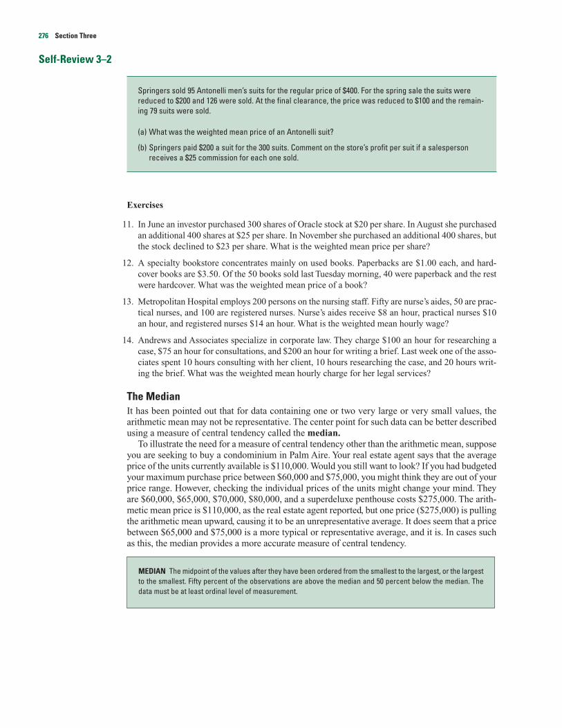
Springers sold 95 Antonelli men’s suits for the regular price of $400. For the spring sale the suits werereduced to $200 and 126 were sold. At the final clearance, the price was reduced to $100 and the remain-ing 79 suits were sold.
(a) What was the weighted mean price of an Antonelli suit?
(b) Springers paid $200 a suit for the 300 suits. Comment on the store’s profit per suit if a salespersonreceives a $25 commission for each one sold.
276 Section Three
The median price of the units available is $70,000. To determine this, we ordered the pricesfrom low ($60,000) to high ($275,000) and selected the middle value ($70,000).
Prices Ordered Prices Orderedfrom Low to High from High to Low
$ 60,000 $275,000
65,000 80,000
70,000 ← Median → 70,000
80,000 65,000
275,000 60,000
Note that there are the same number of prices below the median of $70,000 as above it. Themedian is, therefore, unaffected by extremely low or high observations. Had the highest pricebeen $90,000, or $300,000, or even $1 million, the median price would still be $70,000. Likewise,had the lowest price been $20,000 or $50,000, the median price would still be $70,000.
In the previous illustration there is an odd number of observations (five). How is the mediandetermined for an even number of observations? As before, the observations are ordered. Then theusual practice is to find the arithmetic mean of the two middle observations. Note that for an evennumber of observations, the median may not be one of the given values.
Example
Solution
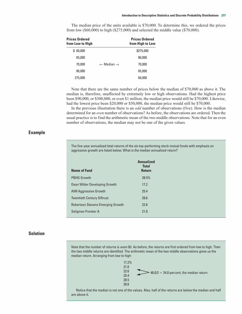
Note that the number of returns is even (6). As before, the returns are first ordered from low to high. Thenthe two middle returns are identified. The arithmetic mean of the two middle observations gives us themedian return. Arranging from low to high:
17.2%21.022.625.4
48.0/2 � 24.0 percent, the median return
28.528.6
Notice that the median is not one of the values. Also, half of the returns are below the median and halfare above it.
The five-year annualized total returns of the six top-performing stock mutual funds with emphasis onaggressive growth are listed below. What is the median annualized return?
Annualized Total
Name of Fund Return
PBHG Growth 28.5%
Dean Witter Developing Growth 17.2
AIM Aggressive Growth 25.4
Twentieth Century Giftrust 28.6
Robertson Stevens Emerging Growth 22.6
Seligman Frontier A 21.0
Introduction to Descriptive Statistics and Discrete Probability Distributions 277
The major properties of the median are:
1. The median is unique; that is, like the mean, there is only one median for a set of data.
2. It is not affected by extremely large or small values and is therefore a valuable measure of centraltendency when such values do occur.
3. It can be computed for a frequency distribution with an open-ended class if the median does not liein an open-ended class. (We will show the computations for the median of data grouped in a fre-quency distribution shortly.)
4. It can be computed for ratio-level, interval-level, and ordinal-level data. (Recall that ordinal-leveldata can be ranked from low to high — such as the responses “excellent,” “very good,” “good,”“fair,” and “poor” to a question on a marketing survey.) To use a simple illustration, suppose fivepeople rated a new fudge bar. One person thought it was excellent, one rated it very good, onecalled it good, one rated it fair, and one considered it poor. The median response is “good.” Half ofthe responses are above “good”; the other half are below it.
The ModeThe mode is another measure of central tendency.
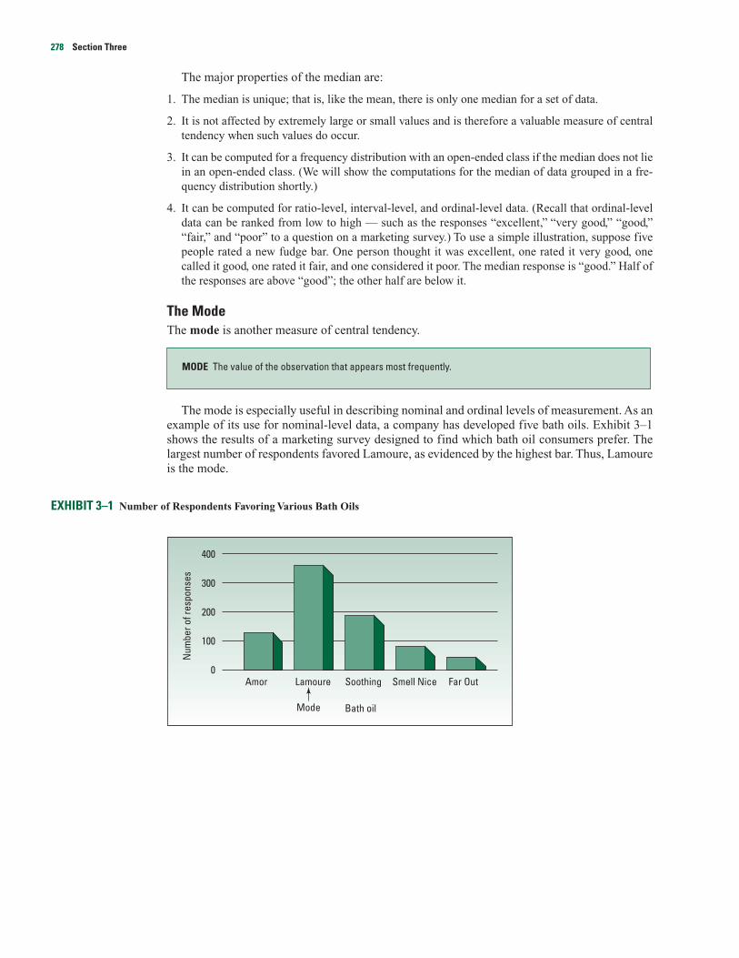
The mode is especially useful in describing nominal and ordinal levels of measurement. As anexample of its use for nominal-level data, a company has developed five bath oils. Exhibit 3–1shows the results of a marketing survey designed to find which bath oil consumers prefer. Thelargest number of respondents favored Lamoure, as evidenced by the highest bar. Thus, Lamoureis the mode.
EXHIBIT 3–1 Number of Respondents Favoring Various Bath Oils
Num
ber o
f res
pons
es
Bath oil
Amor Lamoure Soothing
300
200
100
0
400
Smell Nice Far Out
Mode
MODE The value of the observation that appears most frequently.
278 Section Three

Example
Solution
In summary, we can determine the mode for all levels of data—nominal, ordinal, interval, andratio. The mode also has the advantage of not being affected by extremely high or low values.Like the median, it can be used as a measure of central tendency for distributions with open-ended classes.
The mode does have a number of disadvantages, however, that cause it to be used less fre-quently than the mean or median. For many sets of data, there is no mode because no valueappears more than once. For example, there is no mode for this set of price data: $19, $21, $23,$20, and $18. Since every value is different, however, it could be argued that every value is themode. Conversely, for some data sets there is more than one mode. Suppose the ages of a groupare 22, 26, 27, 27, 31, 35, and 35. Both the ages 27 and 35 are modes. Thus, this grouping of agesis referred to as bimodal (having two modes). One would question the use of two modes to rep-resent the central tendency of this set of age data.
Self-Review 3–3
1. A sample of single persons in Towson, Texas, receiving Social Security payments revealed thesemonthly benefits: $426, $299, $290, $687, $480, $439, and $565.
(a) What is the median monthly benefit?
(b) How many observations are below the median? Above it?
2. The numbers of work stoppages in the automobile industry for selected months are 6, 0, 10, 14, 8, and 0.
(a) What is the median number of stoppages?
(b) How many observations are below the median? Above it?
(c) What is the modal number of work stoppages?
A perusal of the salaries reveals that the annual salary of $60,000 appears more often (six times) than anyother salary. The mode is, therefore, $60,000.
The annual salaries of quality-control managers in selected states are shown below. What is the modalannual salary?
State Salary State Salary State Salary
Arizona $35,000 Illinois $58,000 Ohio $50,000
California 49,100 Louisiana 60,000 Tennessee 60,000
Colorado 60,000 Maryland 60,000 Texas 71,400
Florida 60,000 Massachusetts 40,000 West Virginia 60,000
Idaho 40,000 New Jersey 65,000 Wyoming 55,000
Introduction to Descriptive Statistics and Discrete Probability Distributions 279
Exercises
15. What would you report as the modal value for a set of observations if there were a total of:
a. 10 observations and no two values were the same?
b. 6 observations and they were all the same?
c. 6 observations and the values were 1, 2, 3, 3, 4, and 4?
For exercises 16–19, (a) determine the median and (b) the mode.
16. The following is the number of oil changes for the last seven days at the Jiffy Lube located at thecorner of Elm Street and Pennsylvania Ave.
41 15 39 54 31 15 33
17. The following is the percent change in net income from 2000 to 2001 for a sample of 12 construc-tion companies in Denver.
5 1 �10 �6 5 12 7 8 2 5 �1 11
18. The following are the ages of the 10 people in the video arcade at the Southwyck Shopping Mallat 10 A.M. this morning.
12 8 17 6 11 14 8 17 10 8
19. Listed below are several indicators of long-term economic growth in the United States. The pro-jections are through the year 2005.
Economic Indicator Percent Change Economic Indicator Percent Change
Inflation 4.5 Real GNP 2.9
Exports 4.7 Investment (residential) 3.6
Imports 2.3 Investment (nonresidential) 2.1
Real disposable income 2.9 Productivity (total) 1.4
Consumption 2.7 Productivity (manufacturing) 5.2
a. What is the median percent change?
b. What is the modal percent change?
20. Listed below are the total automobile sales (in millions) in the United States for the last 14 years.During this period, what was the median number of automobiles sold? What is the mode?
9 . 0 8 . 5 8 . 0 9 . 1 1 0 . 3 1 1 . 0 1 1 . 5 1 0 . 3 1 0 . 5 9 . 8 9 . 3 8 . 2 8 . 2 8 . 5
Computer SolutionWe can use a computer software package to find many measures of central tendency.
280 Section Three

Example
Solution
The mean and the median selling prices are reported in the following Excel output. (Remember: Theinstructions to create the output appear in the Computer Commands section to follow.) There are 80 vehi-cles in the study, so the calculations with a calculator would be tedious and prone to error.
The mean selling price is $20,218 and the median is $19,831. These two values are less than $400apart. So either value is reasonable. We can also see from the Excel output that there were 80 vehiclessold and their total price is $1,617,453.
What can we conclude? The typical vehicle sold for about $20,000. Mr. Whitner might use this value inhis revenue projections. For example, if the dealership could increase the number sold in a month from 80to 90, this would result in an additional $200,000 of revenue, found by 10 � $20,000.
Exhibit 3–2 shows the prices of the 80 vehicles sold last month at Whitner Pontiac. Determine the mean and the median sellingprice.
EXHIBIT 3–2 Prices of Vehicles Sold Last Month at Whitner Pontiac
$20,197 $20,372 $17,454 $20,591 $23,651 $24,453 $14,266 $15,021 $25,683 $27,872
16,587 20,169 32,851 16,251 17,047 21,285 21,324 21,609 25,670 12,546
12,935 16,873 22,251 22,277 25,034 21,533 24,443 16,889 17,004 14,357
17,155 16,688 20,657 23,613 17,895 17,203 20,765 22,783 23,661 29,277Lowest
17,642 18,981 21,052 22,799 12,794 15,263 32,925 14,399 14,968 17,356
18,442 18,722 16,331 19,817 16,766 17,633 17,962 19,845 23,285 24,896
26,076 29,492 15,890 18,740 19,374 21,571 22,449 25,337 17,642 20,613
21,220 27,655 19,442 14,891 17,818 23,237 17,445 18,556 18,639 21,296
Highest
Introduction to Descriptive Statistics and Discrete Probability Distributions 281

The Geometric MeanThe geometric mean is useful in finding the average of percentages, ratios, indexes, or growth
rates. It has a wide application in business and economics because we are often interested in find-ing the percentage changes in sales, salaries, or economic figures, such as the Gross NationalProduct, which compound or build on each other. The geometric mean of a set of n positive num-bers is defined as the nth root of the product of n values. The formula for the geometric mean iswritten:
GEOMETRIC MEAN GM � [3–4]
The geometric mean will always be less than or equal to (never more than) the arithmetic mean.Note also that all the data values must be positive to determine the geometric mean.
As a brief example of the interpretation of the geometric mean, suppose you receive a 5 per-cent increase in salary this year and a 15 percent increase next year. The average percent increaseis 9.886, not 10.0. Why is this so? We begin by calculating the geometric mean. Recall, for exam-ple, that a 5 percent increase in salary is 105 or 1.05. We will write it as 1.05.
GM � � 1.09886
This can be verified by assuming that your monthly earning was $3,000 to start and you receivedtwo increases of 5 percent and 15 percent.
Your total salary raise is $622.50. This is equivalent to:
The following example shows the geometric mean of several percentages.
Example
Solution
The geometric mean is 3.46 percent, found by
GM � � �
The geometric mean is the fourth root of 144 or 3.46.1 The geometric mean profit is 3.46 percent.
The arithmetic mean profit is 3.75 percent, found by (3 � 2 � 4 � 6)/4. Although the profit of 6 per-cent is not extremely large, it draws the arithmetic mean upward. The geometric mean of 3.46 gives amore conservative profit figure because it is not being drawn by the large value. It will always, in fact, beless than or equal to the arithmetic mean.
�4 144�4 (3)(2)(4)(6)�n (X1)(X2) · · · (Xn)
The profits earned by Atkins Construction Company on four recent projects were 3 percent, 2 percent, 4percent, and 6 percent. What is the geometric mean profit?
$3,000.00 (.09886) � $296.58$3,296.58 (.09886) � 325.90
$622.48 is about $622.50
Raise 1 � $3,000 (.05) � $150.00Raise 2 � $3,150 (.15) � 472.50
Total $622.50
�(1.05)(1.15)
�n (X1) ) )(X2 ···(Xn
282 Section Three

A second application of the geometric mean is to find an average percent increase over aperiod of time. For example, if you earned $30,000 in 1990 and $50,000 in the year 2000, whatis your annual rate of increase over the period? The rate of increase is determined from the fol-lowing formula.
GM � � 1 [3–5]
In the above box n is the number of periods. An example will show the details of finding the aver-age annual percent increase.
Example
Solution
There are 10 years between 1990 and 2000 so n � 10. The formula (3–5) for the geometric mean asapplied to this type of problem is:
GM � � 1
� � 1 � 1.271 � 1 � 0.271
The final value is .271. So the annual rate of increase is 27.1 percent. This means that the rate of popu-lation growth in Haarlan is 27.1 percent per year.2
Self-Review 3–4
Exercises
21. Compute the geometric mean of the following values: 8, 12, 14, 26, and 5.
22. Compute the geometric mean of the following values: 2, 8, 6, 4, 10, 6, 8, and 4.
1. The annual dividends, in percent, of four oil stocks are: 4.91, 5.75, 8.12, and 21.60.
(a) Find the geometric mean dividend.
(b) Find the arithmetic mean dividend.
(c) Is the arithmetic mean equal to or greater than the geometric mean?
2. Production of Cablos trucks increased from 23,000 units in 1980 to 120,520 units in 2000. Find the geo-metric mean annual percent increase.
�10 222
� n Value at end of periodValue at beginning of period
The population of Haarlan, Alaska, in 1990 was 2 persons, by 2000 it was 22. What is the average annualrate of percentage increase during the period?
� n Value at end of periodValue at beginning of period
Introduction to Descriptive Statistics and Discrete Probability Distributions 283
AVERAGE PERCENT INCREASE OVER TIME

23. Listed below is the percent increase in sales for the MG Corporation over the last 5 years. Deter-mine the geometric mean increase in sales over the period.
9.4 13.8 11.7 11.9 14.7
24. In 1998 revenue from gambling was $651 million. In 2001 the revenue increased to $2.4 billion.What is the geometric mean annual increase for the period?
25. In 1988 hospitals spent 3.9 billion on computer systems. In 2001 this amount increased to $14.0billion. What is the geometric mean annual increase for the period?
26. In 1990 there were 9.19 million cable TV subscribers. By 2000 the number of subscribers increasedto 54.87 million. What is the geometric mean annual increase for the period?
27. In 1996 there were 42.0 million pager subscribers. By 2001 the number of subscribers increased to70.0 million. What is the geometric mean annual increase for the period?
28. The information below shows the cost for a year of college in public and private colleges in 1990and 1998. What is the geometric mean annual increase for the period for the two types of colleges?Compare the rates of increase.
Type of College 1990 1998
Public $ 4,975 $ 7,628
Private 12,284 19,143
Frequency DistributionWe can use descriptive statistics to organize data in various ways to point out where the data val-ues tend to concentrate and help distinguish the largest and the smallest values. One procedure wemight use to describe a set of data is a frequency distribution.
Graphic Presentation of a Frequency DistributionSales managers, stock analysts, hospital administrators, and other busy executives often need aquick picture of the trends in sales, stock prices, or hospital costs. These trends can often bedepicted by the use of charts and graphs. Three charts that will help portray a frequency distribu-tion graphically are the histogram, the frequency polygon, and the cumulative frequency polygon.
Histogram
One of the most common ways to portray a frequency distribution is a histogram.
Thus, a histogram describes a frequency distribution using a series of adjacent rectangles, wherethe height of each rectangle is proportional to the frequency the class represents. The construc-tion of a histogram is best illustrated by reintroducing the prices of the 80 vehicles sold last monthat Whitner Pontiac.
HISTOGRAM A graph in which the classes are marked on the horizontal axis and the class frequencies on thevertical axis. The class frequencies are represented by the heights of the bars, and the bars are drawn adjacentto each other.
FREQUENCY DISTRIBUTION A grouping of data into mutually exclusive classes showing the number of obser-vations in each.
284 Section Three
Example
Solution
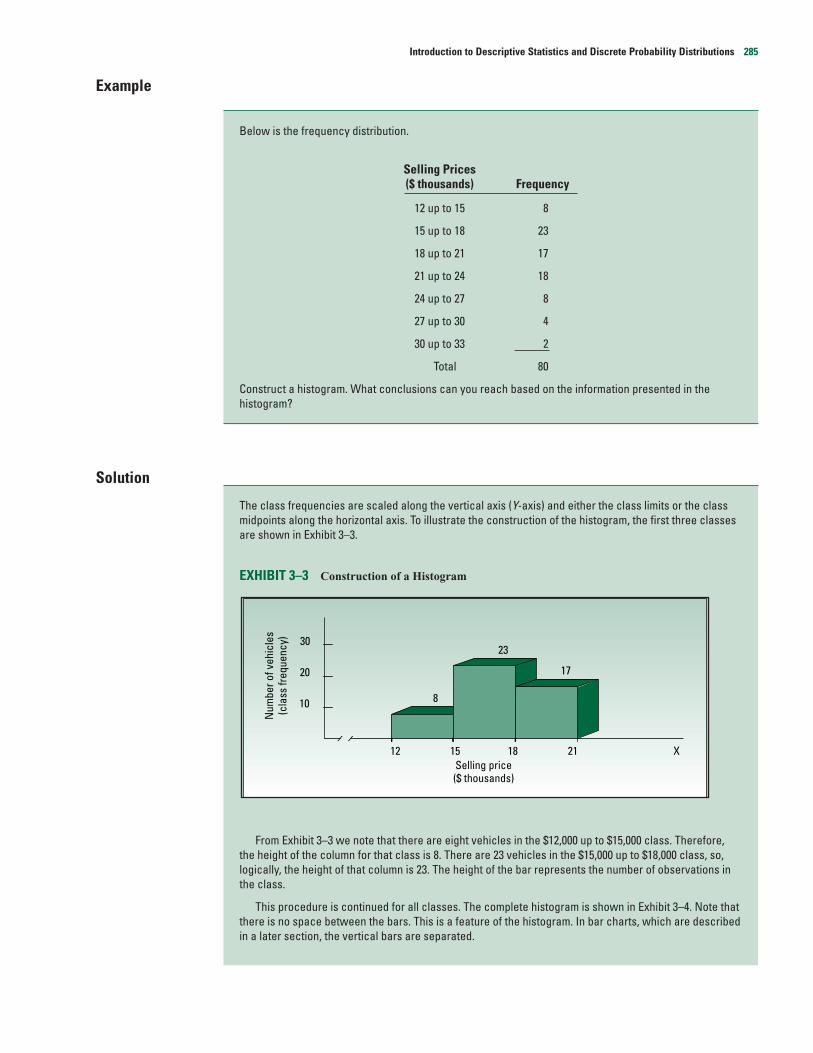
The class frequencies are scaled along the vertical axis (Y-axis) and either the class limits or the classmidpoints along the horizontal axis. To illustrate the construction of the histogram, the first three classesare shown in Exhibit 3–3.
EXHIBIT 3–3 Construction of a Histogram
From Exhibit 3–3 we note that there are eight vehicles in the $12,000 up to $15,000 class. Therefore,the height of the column for that class is 8. There are 23 vehicles in the $15,000 up to $18,000 class, so,logically, the height of that column is 23. The height of the bar represents the number of observations inthe class.
This procedure is continued for all classes. The complete histogram is shown in Exhibit 3–4. Note thatthere is no space between the bars. This is a feature of the histogram. In bar charts, which are describedin a later section, the vertical bars are separated.
12 15 18 21 X
Num
ber o
f veh
icle
s(c
lass
freq
uenc
y)
10
20
30
Selling price($ thousands)
23
17
8
Below is the frequency distribution.
Selling Prices($ thousands) Frequency
12 up to 15 8
15 up to 18 23
18 up to 21 17
21 up to 24 18
24 up to 27 8
27 up to 30 4
30 up to 33 2
Total 80
Construct a histogram. What conclusions can you reach based on the information presented in the histogram?
Introduction to Descriptive Statistics and Discrete Probability Distributions 285
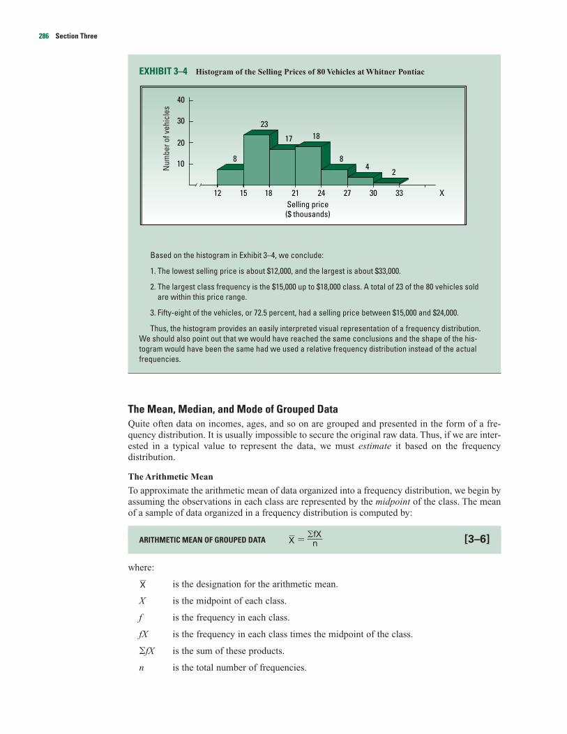
EXHIBIT 3–4 Histogram of the Selling Prices of 80 Vehicles at Whitner Pontiac
Based on the histogram in Exhibit 3–4, we conclude:
1. The lowest selling price is about $12,000, and the largest is about $33,000.
2. The largest class frequency is the $15,000 up to $18,000 class. A total of 23 of the 80 vehicles soldare within this price range.
3. Fifty-eight of the vehicles, or 72.5 percent, had a selling price between $15,000 and $24,000.
Thus, the histogram provides an easily interpreted visual representation of a frequency distribution.We should also point out that we would have reached the same conclusions and the shape of the his-togram would have been the same had we used a relative frequency distribution instead of the actualfrequencies.
The Mean, Median, and Mode of Grouped DataQuite often data on incomes, ages, and so on are grouped and presented in the form of a fre-quency distribution. It is usually impossible to secure the original raw data. Thus, if we are inter-ested in a typical value to represent the data, we must estimate it based on the frequencydistribution.
The Arithmetic Mean
To approximate the arithmetic mean of data organized into a frequency distribution, we begin byassuming the observations in each class are represented by the midpoint of the class. The meanof a sample of data organized in a frequency distribution is computed by:
ARITHMETIC MEAN OF GROUPED DATA � [3–6]
where:
is the designation for the arithmetic mean.
X is the midpoint of each class.
f is the frequency in each class.
fX is the frequency in each class times the midpoint of the class.
�fX is the sum of these products.
n is the total number of frequencies.
X
�fXnX
12 15 18 21
10
30
20
Selling price($ thousands)
23
17 18
84
2
8
24 27 30 33 X
40
Num
ber o
f veh
icle
s
286 Section Three
Example
Solution
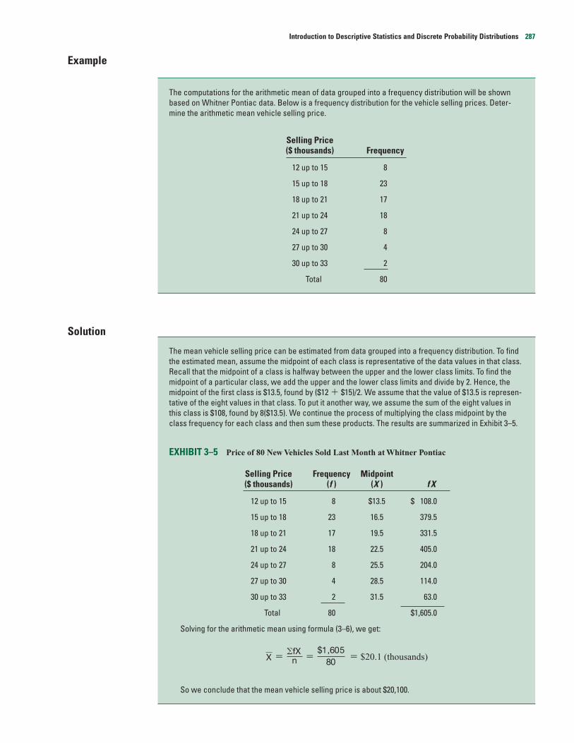
The mean vehicle selling price can be estimated from data grouped into a frequency distribution. To findthe estimated mean, assume the midpoint of each class is representative of the data values in that class.Recall that the midpoint of a class is halfway between the upper and the lower class limits. To find themidpoint of a particular class, we add the upper and the lower class limits and divide by 2. Hence, themidpoint of the first class is $13.5, found by ($12 � $15)/2. We assume that the value of $13.5 is represen-tative of the eight values in that class. To put it another way, we assume the sum of the eight values inthis class is $108, found by 8($13.5). We continue the process of multiplying the class midpoint by theclass frequency for each class and then sum these products. The results are summarized in Exhibit 3–5.
EXHIBIT 3–5 Price of 80 New Vehicles Sold Last Month at Whitner Pontiac
Selling Price Frequency Midpoint($ thousands) (f ) (X ) f X
12 up to 15 8 $13.5 $ 108.0
15 up to 18 23 16.5 379.5
18 up to 21 17 19.5 331.5
21 up to 24 18 22.5 405.0
24 up to 27 8 25.5 204.0
27 up to 30 4 28.5 114.0
30 up to 33 2 31.5 63.0
Total 80 $1,605.0
Solving for the arithmetic mean using formula (3–6), we get:
� � � $20.1 (thousands)
So we conclude that the mean vehicle selling price is about $20,100.
$1,60580
�fXnX
The computations for the arithmetic mean of data grouped into a frequency distribution will be shownbased on Whitner Pontiac data. Below is a frequency distribution for the vehicle selling prices. Deter-mine the arithmetic mean vehicle selling price.
Selling Price($ thousands) Frequency
12 up to 15 8
15 up to 18 23
18 up to 21 17
21 up to 24 18
24 up to 27 8
27 up to 30 4
30 up to 33 2
Total 80
Introduction to Descriptive Statistics and Discrete Probability Distributions 287
The mean of data grouped into a frequency distribution may be different from that of raw data.The grouping results in some loss of information. In the vehicle selling price problem, the meanof the raw data, reported in the previous Excel output is $20,218. This value is quite close to thatestimated mean just computed. The difference is $118 or about 0.58 percent.
Self-Review 3–5
Exercises
29. When we compute the mean of a frequency distribution, why do we refer to this as an estimatedmean?
30. Determine the estimated mean of the following frequency distribution.
Class Frequency
0 up to 5 2
5 up to 10 7
10 up to 15 12
15 up to 20 6
20 up to 25 3
31. Determine the estimated mean of the following frequency distribution.
Class Frequency
20 up to 30 7
30 up to 40 12
40 up to 50 21
50 up to 60 18
60 up to 70 12
32. The selling prices of a sample of 60 antiques sold in Erie, Pennsylvania, last month were organizedinto the following frequency distribution. Estimate the mean selling price.
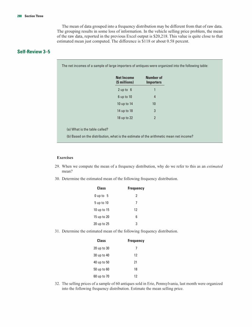
The net incomes of a sample of large importers of antiques were organized into the following table:
Net Income Number of($ millions) Importers
2 up to 6 1
6 up to 10 4
10 up to 14 10
14 up to 18 3
18 up to 22 2
(a) What is the table called?
(b) Based on the distribution, what is the estimate of the arithmetic mean net income?
288 Section Three

Selling Price($ thousands) Frequency
70 up to 80 3
80 up to 90 7
90 up to 100 18
100 up to 110 20
110 up to 120 12
33. FM radio station WLQR recently changed its format from easy listening to contemporary. A recentsample of 50 listeners revealed the following age distribution. Estimate the mean age of the listeners.
Age Frequency
20 up to 30 1
30 up to 40 15
40 up to 50 22
50 up to 60 8
60 up to 70 4
34. Advertising expenses are a significant component of the cost of goods sold. Listed below is a fre-quency distribution showing the advertising expenditures for 60 manufacturing companies locatedin the Southwest. Estimate the mean advertising expense.
AdvertisingExpenditure Number of($ millions) Companies
25 up to 35 5
35 up to 45 10
45 up to 55 21
55 up to 65 16
65 up to 75 8
Total 60
The Median
Recall that the median is defined as the value below which half of the values lie and above whichthe other half of the values lie. Since the raw data have been organized into a frequency distribu-tion, some of the information is not identifiable. As a result we cannot determine the exact median.It can be estimated, however, by (1) locating the class in which the median lies and then (2) inter-polating within that class to arrive at the median. The rationale for this approach is that the mem-bers of the median class are assumed to be evenly spaced throughout the class. The formula is:
MEDIAN OF GROUPED DATA Median � L � (i ) [3–7]n2
� CF
f
Introduction to Descriptive Statistics and Discrete Probability Distributions 289
where:
L is the lower limit of the class containing the median.
n is the total number of frequencies.
f is the frequency in the median class.
CF is the cumulative number of frequencies in all the classes preceding the classcontaining the median.
i is the width of the class in which the median lies.
First, we shall estimate the median by locating the class in which it falls and interpolating.Then the formula for the median will be applied to check our answer.
Example
Solution
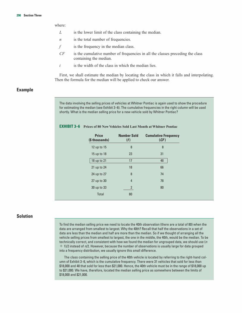
To find the median selling price we need to locate the 40th observation (there are a total of 80) when thedata are arranged from smallest to largest. Why the 40th? Recall that half the observations in a set ofdata are less than the median and half are more than the median. So if we thought of arranging all thevehicle selling prices from smallest to largest, the one in the middle, the 40th, would be the median. To betechnically correct, and consistent with how we found the median for ungrouped data, we should use (n� 1)/2 instead of n/2. However, because the number of observations is usually large for data groupedinto a frequency distribution, we usually ignore this small difference.
The class containing the selling price of the 40th vehicle is located by referring to the right-hand col-umn of Exhibit 3–6, which is the cumulative frequency. There were 31 vehicles that sold for less than$18,000 and 48 that sold for less than $21,000. Hence, the 40th vehicle must be in the range of $18,000 upto $21,000. We have, therefore, located the median selling price as somewhere between the limits of$18,000 and $21,000.
The data involving the selling prices of vehicles at Whitner Pontiac is again used to show the procedurefor estimating the median (see Exhibit 3–6). The cumulative frequencies in the right column will be usedshortly. What is the median selling price for a new vehicle sold by Whitner Pontiac?
EXHIBIT 3–6 Prices of 80 New Vehicles Sold Last Month at Whitner Pontiac
Price Number Sold Cumulative Frequency($ thousands) (f ) (CF )
12 up to 15 8 8
15 up to 18 23 31
18 up to 21 17 48
21 up to 24 18 66
24 up to 27 8 74
27 up to 30 4 78
30 up to 33 2 80
Total 80
290 Section Three

To locate the median more precisely, we need to interpolate in this class containing the median. Recallthat there are 17 vehicles in the “$18,000 up to $21,000” class. Assume the selling prices are evenly distrib-uted between the lower ($18,000) and the upper ($21,000) class limits. There are nine vehicle selling pricesbetween the 31st and the 40th vehicle, found by 40 � 31. The median is, therefore, 9/17 of the distancebetween $18,000 and $21,000. See Exhibit 3–7. The class width is $3,000 and 9/17 of $3,000 is $1,588. Weadd $1,588 to the lower class limit of $18,000, so the estimated median vehicle selling price is $19,588.
EXHIBIT 3–7 Location of the Median
We could also use formula (3–7) to determine the median of data grouped into a frequency distribu-tion, where L is the lower limit of the class containing the median, which is $18,000. There are 80 vehiclessold, so n � 80. CF is the cumulative number of vehicles sold preceding the median class (31), f is the fre-quency of the number of observations in the median class (17), and i is the interval of the class containingthe median ($3,000). Substituting these values:
Median � L � ( i )
� $18,000 � ($3,000)
� $18,000 � $1,588 � $19,588
The assumption underlying the approximation of the median, that the frequencies in the median classare evenly distributed between $18,000 and $21,000, may not be exactly correct. Therefore, it is safer tosay that about half of the selling prices are less than $19,588 and about half are more. The median esti-mated from grouped data and the median determined from raw data are usually not exactly equal. In thiscase, the median computed from raw data using Excel is $19,831 and the median estimated from the fre-quency distribution is $19,588. The difference in the two estimates is $243 or about 1 percent.
A final note: The median is based only on the frequencies and the class limits of the medianclass. The open-ended classes that occur at the extremes are rarely needed. Therefore, the medianof a frequency distribution having open ends can be determined. The arithmetic mean of a fre-quency distribution with an open-ended class cannot be accurately computed — unless, of course,the midpoints of the open-ended classes are estimated. Further, the median can be determined ifpercentage frequencies are given instead of the actual frequencies. This is because the median isthe value with 50 percent of the distribution above it and 50 percent below it and does not dependon actual counts. The percents are considered substitutes for the actual frequencies. In a sense,they are actual frequencies whose total is 100.0.
The Mode
Recall that the mode is defined as the value that occurs most often. For data grouped into a fre-quency distribution, the mode can be approximated by the midpoint of the class containing thelargest number of class frequencies. For Exercise 2 in Self-Review 3–6, the modal net salesare found by first locating the class containing the greatest number of percents. It is the $7 mil-lion up to $10 million class because it has the largest percentage (40). The midpoint of that
802
� 31
17
n2
� CF
f
484031 Vehicles
$21,000 Selling price? Median$18,000
Introduction to Descriptive Statistics and Discrete Probability Distributions 291

class ($8.5 million) is the estimated mode. This indicates that more stamping plants had netsales of $8.5 million than any other amount.
Two values may occur a large number of times. The distribution is then called bimodal. Sup-pose the ages of a sample of workers are 22, 27, 30, 30, 30, 30, 34, 58, 60, 60, 60, 60, and 65. Thetwo modes are 30 years and 60 years. Often two points of concentration develop because the pop-ulation being sampled is probably not homogeneous. In this illustration, the population might becomposed of two distinct groups—one a group of relatively young employees who have beenrecently hired to meet the increased demand for a product, and the other a group of older employ-ees who have been with the company a long time.
If the set of data has more than two modes, the distribution is referred to as being multimodal.In such cases we would probably not consider any of the modes as being representative of the cen-tral value of the data.
Self-Review 3–6
Exercises
35. Refer to Exercise 30. Compute the median. What is the modal value?
36. Refer to Exercise 31. Compute the median. What is the modal value?
37. The chief accountant at Betts Machine, Inc. wants to prepare a report on the company’s accountsreceivable. Below is a frequency distribution showing the amounts outstanding.
1. A sample of the daily production of transceivers at Scott Electronics was organized into the followingdistribution. Estimate the median daily production.
DailyProduction Frequency
80 up to 90 5
90 up to 100 9
100 up to 110 20
110 up to 120 8
120 up to 130 6
130 up to 140 2
2. The net sales of a sample of small stamping plants were organized into the following percentage fre-quency distribution. What is the estimated median net sales?
Net Sales Percent of($ millions) Total
1 up to 4 13
4 up to 7 14
7 up to 10 40
10 up to 13 23
13 and greater 10
292 Section Three
Amount Frequency
$ 0 up to $ 2,000 4
$ 2,000 up to $ 4,000 15
$ 4,000 up to $ 6,000 18
$ 6,000 up to $ 8,000 10
$ 8,000 up to $10,000 4
$10,000 up to $12,000 3
a. Determine the median amount.
b. What is the modal amount owed?
38. At the present time there are about 1.2 million enlisted men and women on active duty in the UnitedStates Army, Navy, Marines, and Air Force. Shown below is a percent breakdown by age. Deter-mine the median age of enlisted personnel on active duty. What is the mode?
Age (years) Percent
Up to 20 15
20 up to 25 33
25 up to 30 19
30 up to 35 17
35 up to 40 11
40 up to 45 4
45 or more 1
39. The following graphic appeared in USA Today and is available at the Website: http://www.usatoday.com/snapshot/news/snapmdex.htm. It reports the number of pages printed per day by office work-ers. Based on this information, what is the median number of pages printed per day per employee?
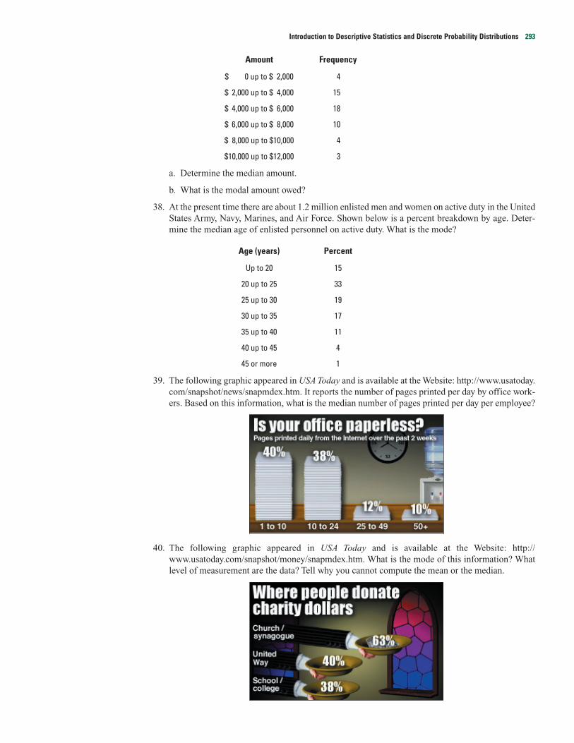
40. The following graphic appeared in USA Today and is available at the Website: http://www.usatoday.com/snapshot/money/snapmdex.htm. What is the mode of this information? Whatlevel of measurement are the data? Tell why you cannot compute the mean or the median.
Introduction to Descriptive Statistics and Discrete Probability Distributions 293
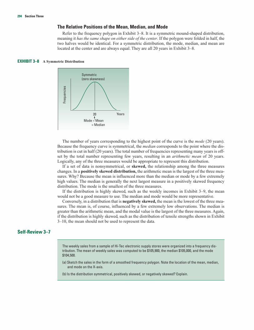
The Relative Positions of the Mean, Median, and ModeRefer to the frequency polygon in Exhibit 3–8. It is a symmetric mound-shaped distribution,
meaning it has the same shape on either side of the center. If the polygon were folded in half, thetwo halves would be identical. For a symmetric distribution, the mode, median, and mean arelocated at the center and are always equal. They are all 20 years in Exhibit 3–8.
EXHIBIT 3–8 A Symmetric Distribution
The number of years corresponding to the highest point of the curve is the mode (20 years).Because the frequency curve is symmetrical, the median corresponds to the point where the dis-tribution is cut in half (20 years). The total number of frequencies representing many years is off-set by the total number representing few years, resulting in an arithmetic mean of 20 years.Logically, any of the three measures would be appropriate to represent this distribution.
If a set of data is nonsymmetrical, or skewed, the relationship among the three measureschanges. In a positively skewed distribution, the arithmetic mean is the largest of the three mea-sures. Why? Because the mean is influenced more than the median or mode by a few extremelyhigh values. The median is generally the next largest measure in a positively skewed frequencydistribution. The mode is the smallest of the three measures.
If the distribution is highly skewed, such as the weekly incomes in Exhibit 3–9, the meanwould not be a good measure to use. The median and mode would be more representative.
Conversely, in a distribution that is negatively skewed, the mean is the lowest of the three mea-sures. The mean is, of course, influenced by a few extremely low observations. The median isgreater than the arithmetic mean, and the modal value is the largest of the three measures. Again,if the distribution is highly skewed, such as the distribution of tensile strengths shown in Exhibit3–10, the mean should not be used to represent the data.
Self-Review 3–7
The weekly sales from a sample of Hi-Tec electronic supply stores were organized into a frequency dis-tribution. The mean of weekly sales was computed to be $105,900, the median $105,000, and the mode$104,500.
(a) Sketch the sales in the form of a smoothed frequency polygon. Note the location of the mean, median,and mode on the X-axis.
(b) Is the distribution symmetrical, positively skewed, or negatively skewed? Explain.
20
Mode = Mean = Median
Symmetric(zero skewness)
Years
Freq
uenc
ies
294 Section Three

Summary
I. A measure of location is a value used to describe the center of a set of data.
A. The arithmetic mean is the most widely reported measure of location.
1. It is calculated by adding the values of the observations and dividing by the total number ofobservations.
a. The formula for a population mean of ungrouped or raw data is:
� � [3–1]
b. The formula for the mean of a sample is
� [3–2]
c. For data grouped into a frequency distribution, the formula is:
� [3–6]
2. The major characteristics of the arithmetic mean are:
a. At least the interval scale of measurement is required.
b. All the data values are used in the calculation.
c. A set of data has only one mean. That is, it is unique.
d. The sum of the deviations from the mean equals 0.
B. The weighted mean is found by multiplying each observation by its corresponding weight.
1. The formula for determining the weighted mean is:
w � [3–3]
2. It is a special case of the arithmetic mean.
C. The geometric mean is the nth root of the product of n values.
w1
w1 w2 w3 wn
X1 � w2 X2 � w3 X3 � · · ·� wn Xn
� � � ···�X
�fXnX
�XN
X
�XN
EXHIBIT 3–10 A Negatively Skewed DistributionEXHIBIT 3–9 A Positively Skewed Distribution
Mode 3,000
Tensile strength
Freq
uenc
y
Median 1,800
Mean 1,200
Skewed to the left(negatively skewed)
Mode$300
Weekly income
Freq
uenc
y
Median $500
Mean $600
Skewed to the right(positively skewed)
Introduction to Descriptive Statistics and Discrete Probability Distributions 295

1. The formula for the geometric mean is:
GM � [3–4]
2. The geometric mean is also used to find the rate of change from one period to another.
GM � � 1 [3–5]
3. The geometric mean is always equal to or less than the arithmetic mean.
D. The median is the value in the middle of a set of ordered data.
1. To find the median, sort the observations from smallest to largest and identify the middle value.
2. The formula for estimating the median from grouped data is:
Median � L � (i ) [3–7]
3. The major characteristics of the median are:
a. At least the ordinal scale of measurement is required.
b. It is not influenced by extreme values.
c. Fifty percent of the observations are larger than the median.
d. It is unique to a set of data.
E. The mode is the value that occurs most often in a set of data.
1. The mode can be found for nominal level data.
2. A set of data can have more than one mode.
Pronunciation Key
SYMBOL MEANING PRONUNCIATION
� Population mean mu
� Operation of adding sigma
�X Adding a group of values sigma X
Sample mean X bar
w Weighted mean X bar sub w
GM Geometric mean G M
�f X Adding the product of the sigma f Xfrequencies and the classmidpoints
X
X
n2
� CF
f
� n Value at end of periodValue at beginning of period
�n (X1) ) )(X2 · · · (Xn
296 Section Three

Snapshot 3–2Most colleges report the “average class size.” This information can be misleading because average class size can be found several ways. If we findthe number of students in each class at a particular university, the result is the mean number of students per class. If we compiled a list of the classsizes for each student and find the mean class size, we might find the mean to be quite different. One school found the mean number of students ineach of their 747 classes to be 40. But when they found the mean from a list of the class sizes of each student it was 147. Why the disparity? Becausethere are few students in the small classes and a larger number of students in the larger class, which has the effect of increasing the mean classsize when it is calculated this way. A school could reduce this mean class size for each student by reducing the number of students in each class.That is, cut out the large freshman lecture classes.
Exercises
41. The accounting firm of Crawford and Associates has five senior partners. Yesterday the senior part-ners saw six, four, three, seven, and five clients, respectively.
a. Compute the mean number and median number of clients seen by a partner.
b. Is the mean a sample mean or a population mean?
c. Verify that �(X � �) � 0.
42. Owens Orchards sells apples in a large bag by weight. A sample of seven bags contained the fol-lowing numbers of apples: 23, 19, 26, 17, 21, 24, 22.
a. Compute the mean number and median number of apples in a bag.
b. Verify that �(X � ) � 0.
43. A sample of households that subscribe to the United Bell Phone Company revealed the followingnumbers of calls received last week. Determine the mean and the median number of calls received.
52 43 30 38 30 42 12 46 39 37
34 46 32 18 41 5
44. The Citizens Banking Company is studying the number of times the ATM, located in a LoblawsSupermarket, is used per day. Following are the numbers of times the machine was used over eachof the last 30 days. Determine the mean number of times the machine was used per day.
83 64 84 76 84 54 75 59 70 61
63 80 84 73 68 52 65 90 52 77
95 36 78 61 59 84 95 47 87 60
45. Listed below is the number of lampshades produced during the last 50 days at the American Lamp-shade Company in Rockville, GA. Compute the mean.
348 371 360 369 376 397 368 361 374
410 374 377 335 356 322 344 399 362
384 365 380 349 358 343 432 376 347
385 399 400 359 329 370 398 352 396
366 392 375 379 389 390 386 341 351
354 395 338 390 333
X
Introduction to Descriptive Statistics and Discrete Probability Distributions 297

46. Trudy Green works for the True-Green Lawn Company. Her job is to solicit lawn-care business viathe telephone. Listed below are the number of appointments she made in each of the last 25 hoursof calling. What is the arithmetic mean number of appointments she made per hour? What is themedian number of appointments per hour? Write a brief report summarizing the findings.
9 5 2 6 5 6 4 4 7 2 3 6 3
4 4 7 8 4 4 5 5 4 8 3 3
47. The Split-A-Rail Fence Company sells three types of fence to homeowners in suburban Seattle,Washington. Grade A costs $5.00 per running foot to install, Grade B costs $6.50 per running foot,and Grade C, the premium quality, costs $8.00 per running foot. Yesterday, Split-A-Rail installed270 feet of Grade A, 300 feet of Grade B, and 100 feet of Grade C. What was the mean cost per footof fence installed?
48. Rolland Poust is a sophomore in the College of Business at Scandia Tech. Last semester he tookcourses in statistics and accounting, 3 hours each, and earned an A in both. He earned a B in a five-hour history course and a B in a two-hour history of jazz course. In addition, he took a one-hourcourse dealing with the rules of basketball so he could get his license to officiate high school basket-ball games. He got an A in this course. What was his GPA for the semester? Assume that he receives4 points for an A, 3 for a B, and so on. What measure of central tendency did you just calculate?
49. The table below shows the percent of the labor force that is unemployed and the size of the laborforce for three counties in Northwest Ohio. Jon Elsas is the Regional Director of Economic Devel-opment. He must present a report to several companies that are considering locating in NorthwestOhio. What would be an appropriate unemployment rate to show for the entire region?
County Percent Unemployed Size of Workforce
Wood 4.5 15,300
Ottawa 3.0 10,400
Lucas 10.2 150,600
50. Modern Healthcare reported the average patient revenues (in $ millions) for five types of hospitals.What is the median patient revenue?
Patient RevenueHospital Type (millions)
Catholic $46.6
Other church 59.1
Nonprofit 71.7
Public 93.1
For profit 32.4
51. The Bank Rate Monitor reported the following savings rates. What is the median savings rate?
Instrument Savings Rate (percent) Instrument Savings Rate (percent)
Money market mutual fund 3.01 1-year CD 3.51
Bank money market account 2.96 2.5-year CD 4.25
6-month CD 3.25 5-year CD 5.46
298 Section Three

52. The American Automobile Association checks the prices of gasoline before many holiday week-ends. Listed below are the self-service prices for a sample of 15 retail outlets during the May 2000Memorial Day weekend in the Detroit, Michigan, area.
1.44 1.42 1.35 1.39 1.49 1.49 1.41 1.46
1.41 1.49 1.45 1.48 1.39 1.46 1.44
a. What is the arithmetic mean selling price?
b. What is the median selling price?
c. What is the modal selling price?
53. The following table shows major earthquakes by country between 1983 and 1995. Also reported isthe size of the earthquake, as measured on the Richter Scale, and the number of deaths reported.Compute the mean and the median for both the size of the earthquake as measured on the Richterscale and the number of deaths. Which measure of central tendency would you report for each ofthe variables? Tell why.
Country Richter Deaths Country Richter Deaths
Colombia 5.5 250 Iran 7.7 40,000
Japan 7.7 81 Philippines 7.7 1,621
Turkey 7.1 1,300 Pakistan 6.8 1,200
Chile 7.8 146 Turkey 6.2 4,000
Mexico 8.1 4,200 USA 7.5 1
Ecuador 7.3 4,000 Indonesia 7.5 2,000
India 6.5 1,000 India 6.4 9,748
China 7.3 1,000 Indonesia 7.0 215
Armenia 6.8 55,000 Colombia 6.8 1,000
USA 6.9 62 Algeria 6.0 164
Peru 6.3 114 Japan 7.2 5,477
Romania 6.5 8 Russia 7.6 2,000
54. The metropolitan area of Los Angeles–Long Beach, California, is the area expected to show thelargest increase in the number of jobs between 1989 and 2010. The number of jobs is expected toincrease from 5,164,900 to 6,286,800. What is the geometric mean expected yearly rate ofincrease?
55. Wells Fargo Mortgage and Equity Trust gave these occupancy rates in their annual report for vari-ous office income properties the company owns. What is the geometric mean occupancy rate?
Pleasant Hills, California 100%
Lakewood, Colorado 90
Riverside, California 80
Scottsdale, Arizona 20
San Antonio, Texas 62
56. A recent article suggested that if you earn $25,000 a year today and the inflation rate continues at3 percent per year, you’ll need to make $33,598 in 10 years to have the same buying power. Youwould need to make $44,771 if the inflation rate jumped to 6 percent. Confirm that these state-ments are accurate by finding the geometric mean rate of increase.
Introduction to Descriptive Statistics and Discrete Probability Distributions 299
57. Wells Fargo Mortgage and Equity Trust also reported these occupancy rates for some of its indus-trial income properties. What is the geometric mean occupancy rate?
Tucson, Arizona 81%
Irvine, California 100
Carlsbad, California 74
Dallas, Texas 80
58. The 12-month returns on five aggressive-growth mutual funds were 32.2 percent, 35.5 percent,80.0 percent, 60.9 percent, and 92.1 percent. Determine the arithmetic mean and the geometricmean rates of return.
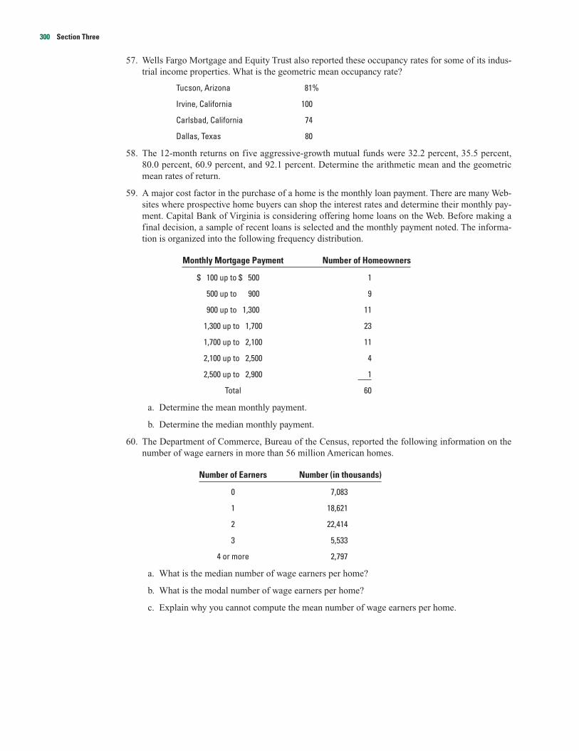
59. A major cost factor in the purchase of a home is the monthly loan payment. There are many Web-sites where prospective home buyers can shop the interest rates and determine their monthly pay-ment. Capital Bank of Virginia is considering offering home loans on the Web. Before making afinal decision, a sample of recent loans is selected and the monthly payment noted. The informa-tion is organized into the following frequency distribution.
Monthly Mortgage Payment Number of Homeowners
$ 100 up to $ 500 1
500 up to 900 9
900 up to 1,300 11
1,300 up to 1,700 23
1,700 up to 2,100 11
2,100 up to 2,500 4
2,500 up to 2,900 1
Total 60
a. Determine the mean monthly payment.
b. Determine the median monthly payment.
60. The Department of Commerce, Bureau of the Census, reported the following information on thenumber of wage earners in more than 56 million American homes.
Number of Earners Number (in thousands)
0 7,083
1 18,621
2 22,414
3 5,533
4 or more 2,797
a. What is the median number of wage earners per home?
b. What is the modal number of wage earners per home?
c. Explain why you cannot compute the mean number of wage earners per home.
300 Section Three

61. ARS Services, Inc. employs 40 electricians, providing service to both residential and commercialaccounts. ARS has been in business since the early 60s and has always advertised prompt and reli-able service. Of concern in recent years is the number of days employees are absent. Below is a fre-quency distribution of the number of days missed by the 40 electricians last year.
Number of Days Missed Number of Electricians
0 up to 3 17
3 up to 6 13
6 up to 9 7
9 up to 12 3
Total 40
a. Determine the mean number of days missed.
b. Determine the median number of days missed.
62. In recent years there has been intense competition for the long distance phone service of residen-tial customers. In an effort to study the actual phone usage of residential customers, an independentconsultant gathered the following data on the number of long distance phone calls per householdfor a sample of 70 households.
Number of Phone Calls Frequency
3 up to 6 5
6 up to 9 19
9 up to 12 20
12 up to 15 20
15 up to 18 4
18 up to 21 2
Total 70
a. Determine the mean number of phone calls per household.
b. Determine the median number of phone calls per household.
63. A sample of 50 American cities with a population between 100,000 and 1,000,000 revealed the fol-lowing frequency distribution for the cost per day for a double occupancy hospital room.
Cost of Hospital Room Frequency
$100 up to $200 1
200 up to 300 9
300 up to 400 20
400 up to 500 15
500 up to 600 5
Total 50
a. Determine the mean cost per day.
b. Determine the median cost per day.
Introduction to Descriptive Statistics and Discrete Probability Distributions 301
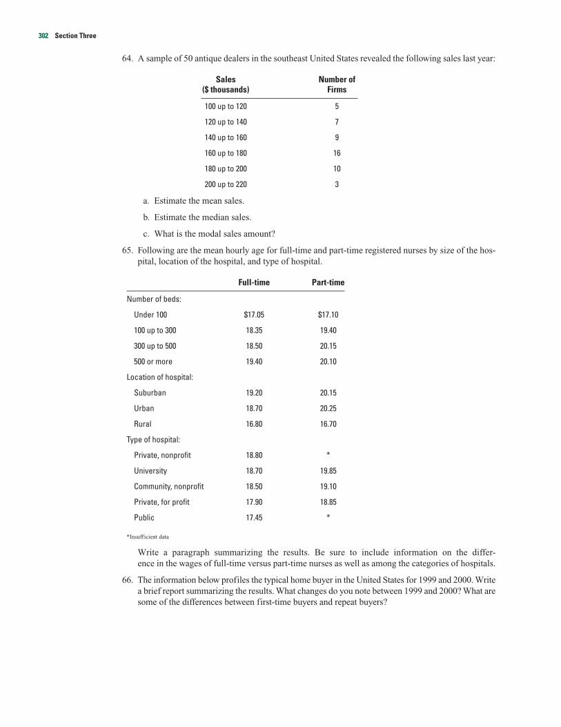
64. A sample of 50 antique dealers in the southeast United States revealed the following sales last year:
Sales Number of($ thousands) Firms
100 up to 120 5
120 up to 140 7
140 up to 160 9
160 up to 180 16
180 up to 200 10
200 up to 220 3
a. Estimate the mean sales.
b. Estimate the median sales.
c. What is the modal sales amount?
65. Following are the mean hourly age for full-time and part-time registered nurses by size of the hos-pital, location of the hospital, and type of hospital.
Full-time Part-time
Number of beds:
Under 100 $17.05 $17.10
100 up to 300 18.35 19.40
300 up to 500 18.50 20.15
500 or more 19.40 20.10
Location of hospital:
Suburban 19.20 20.15
Urban 18.70 20.25
Rural 16.80 16.70
Type of hospital:
Private, nonprofit 18.80 *
University 18.70 19.85
Community, nonprofit 18.50 19.10
Private, for profit 17.90 18.85
Public 17.45 *
*Insufficient data
Write a paragraph summarizing the results. Be sure to include information on the differ-ence in the wages of full-time versus part-time nurses as well as among the categories of hospitals.
66. The information below profiles the typical home buyer in the United States for 1999 and 2000. Writea brief report summarizing the results. What changes do you note between 1999 and 2000? What aresome of the differences between first-time buyers and repeat buyers?
302 Section Three

First-Time Buyers Repeat Buyers
1999 2000 1999 2000
Mean cost of single-family home $156,400 $147,400 $195,300 $212,700
Homes visited before buying 12.9 12.5 15.6 15.7
Mean monthly mortgage payment $950 $945 $1,076 $1,114
Mean age 31.6 31.6 41.0 41.7
exercises.com
67. John Hardy is an investment advisor to several individuals in the Richmond, Virginia, area. He hasbeen asked to compare the profitability of banks in the northeast to those in the southeast. TheYahoo Website allows him to do quick research on the entire industry. Go tohttp://www.yahoo.com, click on Stock Quotes, under Research select By Industry, select Banks,and again under Banks select the Northeast Region. Obtain the earnings per share for the mostrecent quarter for banks in the northeast. Compute the mean earnings per share for the region.Repeat the process for the southeast. That is, in the last step select Southeast as the region. Com-pute the mean earnings per share for banks in this region. Compare the two regions. Which regionseems to be more profitable?
68. One of the most famous averages, the Dow Jones Industrial Average (DJIA), is not really an aver-age. Following is a listing of the 30 stocks that make up the DJIA and their selling prices on July 11,2000. Compute the mean of the 30 stocks. Compare this to the closing price on July 11, 2000 of10,727.19. Then go to the Dow Jones Website and read about the history of this average and thestocks that are currently included in its calculation. To obtain this information go to:http://www.dowjones.com, in the bottom left corner click on About Dow Jones, click on Dow JonesIndustrial Average, and finally click on Stocks. The output is below. Compute the mean of the 30stocks included in the DJIA today and the DJIA with that of July 11, 2000. Has there been a change?
Company Name Symbol Price Weighting %
Alcoa Inc. (AA) 31.6875 1.677
American Express Co. (AXP) 53.5625 2.835
AT & T Corp. (T) 31.8750 1.687
Boeing Co. (BA) 44.1250 2.335
Caterpillar Inc. (CAT) 35.9375 1.902
Citigroup Inc. (C) 65.8750 3.487
Coca-Cola Co. (KO) 56.0000 2.964
DuPont Co. (DD) 46.5625 2.464
Eastman Kodak Co. (EK) 60.6250 3.209
Exxon Mobil Corp. (XOM) 80.4375 4.258
General Electric Co. (GE) 52.7500 2.792
General Motors Corp. (GM) 62.0625 3.285
Home Depot Inc. (HD) 57.1875 3.027
Honeywell International Inc. (HON) 35.8125 1.895
Hewlett-Packard Co. (HWP) 124.8125 6.607
International Business Machines Corp. (IBM) 101.3750 5.366
Introduction to Descriptive Statistics and Discrete Probability Distributions 303
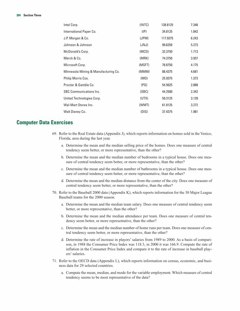
Intel Corp. (INTC) 138.8125 7.348
International Paper Co. (IP) 34.8125 1.842
J.P. Morgan & Co. (JPM) 117.9375 6.243
Johnson & Johnson (JNJ) 99.6250 5.273
McDonald’s Corp. (MCD) 32.3750 1.713
Merck & Co. (MRK) 74.3750 3.937
Microsoft Corp. (MSFT) 78.8750 4.175
Minnesota Mining & Manufacturing Co. (MMM) 88.4375 4.681
Philip Morris Cos. (MO) 25.9375 1.373
Procter & Gamble Co. (PG) 54.5625 2.888
SBC Communications Inc. (SBC) 44.2500 2.342
United Technologies Corp. (UTX) 59.3125 3.139
Wal-Mart Stores Inc. (WMT) 61.8125 3.272
Walt Disney Co. (DIS) 37.4375 1.981
Computer Data Exercises
69. Refer to the Real Estate data (Appendix J), which reports information on homes sold in the Venice,Florida, area during the last year.
a. Determine the mean and the median selling price of the homes. Does one measure of centraltendency seem better, or more representative, than the other?
b. Determine the mean and the median number of bedrooms in a typical house. Does one mea-sure of central tendency seem better, or more representative, than the other?
c. Determine the mean and the median number of bathrooms in a typical house. Does one mea-sure of central tendency seem better, or more representative, than the other?
d. Determine the mean and the median distance from the center of the city. Does one measure ofcentral tendency seem better, or more representative, than the other?
70. Refer to the Baseball 2000 data (Appendix K), which reports information for the 30 Major LeagueBaseball teams for the 2000 season.
a. Determine the mean and the median team salary. Does one measure of central tendency seembetter, or more representative, than the other?
b. Determine the mean and the median attendance per team. Does one measure of central ten-dency seem better, or more representative, than the other?
c. Determine the mean and the median number of home runs per team. Does one measure of cen-tral tendency seem better, or more representative, than the other?
d. Determine the rate of increase in players’ salaries from 1989 to 2000. As a basis of compari-son, in 1988 the Consumer Price Index was 118.3, in 2000 it was 166.9. Compute the rate ofinflation in the Consumer Price Index and compare it to the rate of increase in baseball play-ers’ salaries.
71. Refer to the OECD data (Appendix L), which reports information on census, economic, and busi-ness data for 29 selected countries.
a. Compute the mean, median, and mode for the variable employment. Which measure of centraltendency seems to be most representative of the data?
304 Section Three
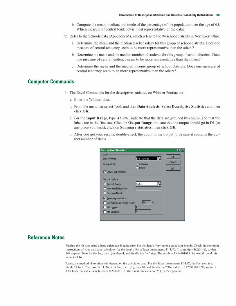
b. Compute the mean, median, and mode of the percentage of the population over the age of 65.Which measure of central tendency is most representative of the data?
72. Refer to the Schools data (Appendix M), which refers to the 94 school districts in Northwest Ohio.
a. Determine the mean and the median teacher salary for this group of school districts. Does onemeasure of central tendency seem to be more representative than the others?
b. Determine the mean and the median number of students for this group of school districts. Doesone measure of central tendency seem to be more representative than the others?
c. Determine the mean and the median income group of school districts. Does one measure ofcentral tendency seem to be more representative than the others?
Computer Commands
1. The Excel Commands for the descriptive statistics on Whitner Pontiac are:
a. Enter the Whitner data.
b. From the menu bar select Tools and then Data Analysis. Select Descriptive Statistics and thenclick OK.
c. For the Input Range, type A1:A81, indicate that the data are grouped by column and that thelabels are in the first row. Click on Output Range, indicate that the output should go in D1 (orany place you wish), click on Summary statistics, then click OK.
d. After you get your results, double-check the count in the output to be sure it contains the cor-rect number of items.
Reference Notes1Finding the nth root using a hand calculator is quite easy, but the details vary among calculator brands. Check the operatinginstructions of your particular calculator for the details. For a Texas Instruments TI-35X, first multiply 3(2)(4)(6), so that144 appears. Next hit the 2nd, then , then 4, and finally the “�” sign. The result is 3.464101615. We would round thisvalue to 3.46.
2Again, the method of solution will depend on the calculator used. For the Texas Instruments TI-35X, the first step is todivide 22 by 2. The result is 11. Next hit 2nd, then , then 10, and finally “�.” The value is 1.270981615. We subtract1.00 from this value, which leaves 0.270981615. We round this value to .271, or 27.1 percent.
�x y
�x y
Introduction to Descriptive Statistics and Discrete Probability Distributions 305

306 Section Three
Answers to Self-Review
3–1 1. (a) �
(b) � � $66,775.
(c) Statistic, because it is a sample value.(d) $66,775. The sample mean is our best estimate
of the population mean.
2. (a) � �
(b) � � � 83
(c) Parameter, because it was computed using allthe population values.
3–2 (a) $237, found by:
� 237
(b) The profit per suit is $12, found by $237 � $200cost � $25 commission. The total profit for the 300suits is $3,600, found by 300 � $12.
3–3 1. (a) $439.(b) 3, 3.
2. (a) 7, found by (6 � 8)/2 � 7.(b) 3, 3.(c) 0.
3–4 1. (a) About 8.39 percent.(b) About 10.095 percent.(c) Greater than, because 10.095 � 8.39.
2. 8.63 percent found by, � 1 � 1.0863 �
1.
3–5 1. (a) Frequency distribution.(b) f X f X
1 4 44 8 32
10 12 1203 16 482 20 40
20 244
� � � $12.2
3–6 1. Production Frequency CF
80 up to 90 5 590 up to 100 9 14
100 up to 110 20 34110 up to 120 8 42120 up to 130 6 48130 up to 140 2 50
50
Median � 100 � (10)
� 100 � 5.5 � 105.5
2. Net Sales Cumulative($ Millions) Percent
$ 1 up to $ 4 134 up to 7 277 up to 10 67
10 up to 13 9013 or greater 100
Median � $7 � ($3)
� $8.725
3–7 (a)
(b) Positively skewed, because the mean is the largestaverage and the mode is the smallest.
Freq
uenc
y
Mod
eM
edia
nM
ean
Weekly sales ($000)
50 � 2740
25 � 1420
$24420
�fXnX
20�120,52023,000
(95 � $400) � (126 � $200 ) � (79 � $100)95 � 126 � 79
4986
�XN
$267, 1004X
�XN
X
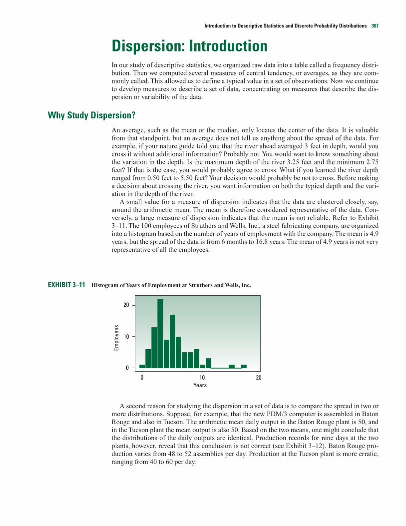
Dispersion: IntroductionIn our study of descriptive statistics, we organized raw data into a table called a frequency distri-bution. Then we computed several measures of central tendency, or averages, as they are com-monly called. This allowed us to define a typical value in a set of observations. Now we continueto develop measures to describe a set of data, concentrating on measures that describe the dis-persion or variability of the data.
Why Study Dispersion?An average, such as the mean or the median, only locates the center of the data. It is valuablefrom that standpoint, but an average does not tell us anything about the spread of the data. Forexample, if your nature guide told you that the river ahead averaged 3 feet in depth, would youcross it without additional information? Probably not. You would want to know something aboutthe variation in the depth. Is the maximum depth of the river 3.25 feet and the minimum 2.75feet? If that is the case, you would probably agree to cross. What if you learned the river depthranged from 0.50 feet to 5.50 feet? Your decision would probably be not to cross. Before makinga decision about crossing the river, you want information on both the typical depth and the vari-ation in the depth of the river.
A small value for a measure of dispersion indicates that the data are clustered closely, say,around the arithmetic mean. The mean is therefore considered representative of the data. Con-versely, a large measure of dispersion indicates that the mean is not reliable. Refer to Exhibit3–11. The 100 employees of Struthers and Wells, Inc., a steel fabricating company, are organizedinto a histogram based on the number of years of employment with the company. The mean is 4.9years, but the spread of the data is from 6 months to 16.8 years. The mean of 4.9 years is not veryrepresentative of all the employees.
44
EXHIBIT 3–11 Histogram of Years of Employment at Struthers and Wells, Inc.
A second reason for studying the dispersion in a set of data is to compare the spread in two ormore distributions. Suppose, for example, that the new PDM/3 computer is assembled in BatonRouge and also in Tucson. The arithmetic mean daily output in the Baton Rouge plant is 50, andin the Tucson plant the mean output is also 50. Based on the two means, one might conclude thatthe distributions of the daily outputs are identical. Production records for nine days at the twoplants, however, reveal that this conclusion is not correct (see Exhibit 3–12). Baton Rouge pro-duction varies from 48 to 52 assemblies per day. Production at the Tucson plant is more erratic,ranging from 40 to 60 per day.
0
0
10
Years
20
Empl
oyee
s
10 20
Introduction to Descriptive Statistics and Discrete Probability Distributions 307

EXHIBIT 3–12 Daily Production of Computers at the Baton Rouge and Tucson Plants
Measures of DispersionWe will consider several measures of dispersion. The range is based on the location of the largestand the smallest values in the data set. The mean deviation, the variance, and the standard devia-tion are all based on deviations from the mean.
Range
The simplest measure of dispersion is the range. It is the difference between the highest and thelowest values in a data set. In the form of an equation:
The range is widely used in statistical process control (SPC) applications.
Example
Solution
The range of the daily production of computers at the Baton Rouge plant is 4, found by the differencebetween the largest daily production of 52 and the smallest of 48. The range in the daily production forthe Tucson plant is 20 computers, found by 60 � 40. We therefore conclude that (1) there is less disper-sion in the daily production in the Baton Rouge plant than in the Tucson plant because the rangeof 4 computers is less than a range of 20 computers, and (2) the production is clustered more closelyaround the mean of 50 at the Baton Rouge plant than at the Tucson plant (because a range of 4 is lessthan a range of 20). Thus, the mean production in the Baton Rouge plant (50 computers) is a more repre-sentative average than the mean of 50 computers for the Tucson plant.
Refer to Exhibit 3–12. Find the range in the number of computers produced for the Baton Rouge and theTucson plants. Interpret the two ranges.
RANGE Range � Highest value � Lowest value [3–8]
48 49 50 51 52 _ X
Baton Rouge
48 49 50 51 52 _ X
Tucson
53 54 55 56 57 58 59 604746454443424140
Daily production
308 Section Three
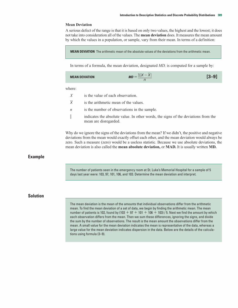
Mean Deviation
A serious defect of the range is that it is based on only two values, the highest and the lowest; it doesnot take into consideration all of the values. The mean deviation does. It measures the mean amountby which the values in a population, or sample, vary from their mean. In terms of a definition:
In terms of a formula, the mean deviation, designated MD, is computed for a sample by:
MEAN DEVIATION MD � [3–9]
where:
X is the value of each observation.
is the arithmetic mean of the values.
n is the number of observations in the sample.
� indicates the absolute value. In other words, the signs of the deviations from themean are disregarded.
Why do we ignore the signs of the deviations from the mean? If we didn’t, the positive and negativedeviations from the mean would exactly offset each other, and the mean deviation would always bezero. Such a measure (zero) would be a useless statistic. Because we use absolute deviations, themean deviation is also called the mean absolute deviation, or MAD. It is usually written MD.
Example
Solution
The mean deviation is the mean of the amounts that individual observations differ from the arithmeticmean. To find the mean deviation of a set of data, we begin by finding the arithmetic mean. The meannumber of patients is 102, found by (103 � 97 � 101 � 106 � 103) / 5. Next we find the amount by whicheach observation differs from the mean. Then we sum these differences, ignoring the signs, and dividethe sum by the number of observations. The result is the mean amount the observations differ from themean. A small value for the mean deviation indicates the mean is representative of the data, whereas alarge value for the mean deviation indicates dispersion in the data. Below are the details of the calcula-tions using formula (3–9).
The number of patients seen in the emergency room at St. Luke’s Memorial Hospital for a sample of 5days last year were: 103, 97, 101, 106, and 103. Determine the mean deviation and interpret.
X
��X � X �n
MEAN DEVIATION The arithmetic mean of the absolute values of the deviations from the arithmetic mean.
Introduction to Descriptive Statistics and Discrete Probability Distributions 309
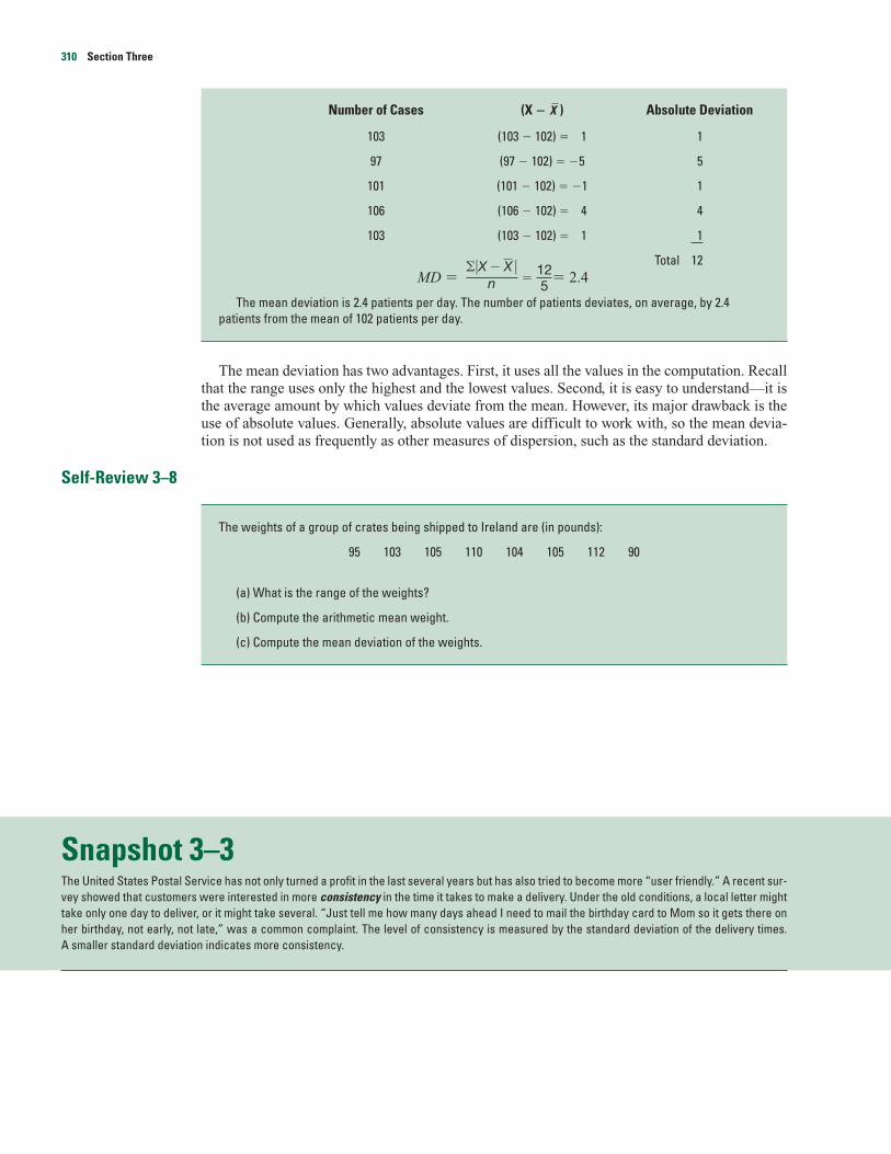
Number of Cases (X � ) Absolute Deviation
103 (103 � 102) � 1 1
97 (97 � 102) � �5 5
101 (101 � 102) � �1 1
106 (106 � 102) � 4 4
103 (103 � 102) � 1 1
Total 12MD � � � 2.4
The mean deviation is 2.4 patients per day. The number of patients deviates, on average, by 2.4patients from the mean of 102 patients per day.
The mean deviation has two advantages. First, it uses all the values in the computation. Recallthat the range uses only the highest and the lowest values. Second, it is easy to understand—it isthe average amount by which values deviate from the mean. However, its major drawback is theuse of absolute values. Generally, absolute values are difficult to work with, so the mean devia-tion is not used as frequently as other measures of dispersion, such as the standard deviation.
Self-Review 3–8
Snapshot 3–3The United States Postal Service has not only turned a profit in the last several years but has also tried to become more “user friendly.” A recent sur-vey showed that customers were interested in more consistency in the time it takes to make a delivery. Under the old conditions, a local letter mighttake only one day to deliver, or it might take several. “Just tell me how many days ahead I need to mail the birthday card to Mom so it gets there onher birthday, not early, not late,” was a common complaint. The level of consistency is measured by the standard deviation of the delivery times.A smaller standard deviation indicates more consistency.
The weights of a group of crates being shipped to Ireland are (in pounds):
95 103 105 110 104 105 112 90
(a) What is the range of the weights?
(b) Compute the arithmetic mean weight.
(c) Compute the mean deviation of the weights.
125
��X � X �n
X
310 Section Three
Exercises
For questions 73 through 78 calculate the (a) range, (b) arithmetic mean, and (c) mean deviation,and (d) interpret the range and the mean deviation.
73. There were five customer service representatives on duty at the Electronic Super Store during lastFriday’s sale. The numbers of VCRs these representatives sold are: 5, 8, 4, 10, and 3.
74. The Department of Statistics at Western State University offers eight sections of basic statistics.Following are the numbers of students enrolled in these sections: 34, 46, 52, 29, 41, 38, 36, and 28.
75. Dave’s Automatic Door installs automatic garage door openers. The following list indicates the num-ber of minutes needed to install a sample of 10 doors: 28, 32, 24, 46, 44, 40, 54, 38, 32, and 42.
76. A sample of eight companies in the aerospace industry was surveyed as to their return on invest-ment last year. The results are (in percent): 10.6, 12.6, 14.8, 18.2, 12.0, 14.8, 12.2, and 15.6.
77. Ten experts rated a newly developed pizza on a scale of 1 to 50. The ratings were: 34, 35, 41, 28,26, 29, 32, 36, 38, and 40.
78. A sample of the personnel files of eight male employees employed by Acme Carpet revealed that,during a six-month period, they lost the following numbers of days due to illness: 2, 0, 6, 3, 10, 4,1, and 2.
Variance and Standard Deviation
The variance and standard deviation are also based on the deviations from the mean.
Note that the variance is non-negative, and it is zero only if all observations are the same.
Population Variance The formulas for the population variance and the sample variance areslightly different. The population variance is considered first. (Recall that a population is thetotality of all observations being studied.) The population variance for ungrouped data, that is,data not tabulated into a frequency distribution, is found by:
POPULATION VARIANCE �2 � [3–10]
where:
�2 is the symbol for the population variance (� is the lower-case Greek lettersigma). It is usually referred to as “sigma squared.”
X is the value of an observation in the population.
� is the arithmetic mean of the population.
N is the number of observations in the population.
�(X � �)2
N
STANDARD DEVIATION The square root of the variance.
VARIANCE The arithmetic mean of the squared deviations from the mean.
Introduction to Descriptive Statistics and Discrete Probability Distributions 311
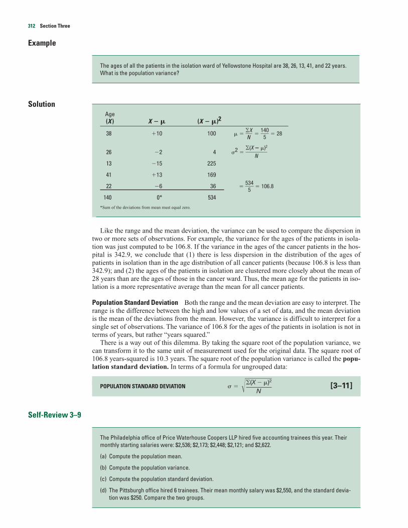
Example
SolutionAge(X ) X � � (X � �)2
38 �10 100 � � � � 28
26 �2 4 �2 �
13 �15 225
41 �13 169
22 �6 36 � � 106.8
140 0* 534
*Sum of the deviations from mean must equal zero.
Like the range and the mean deviation, the variance can be used to compare the dispersion intwo or more sets of observations. For example, the variance for the ages of the patients in isola-tion was just computed to be 106.8. If the variance in the ages of the cancer patients in the hos-pital is 342.9, we conclude that (1) there is less dispersion in the distribution of the ages ofpatients in isolation than in the age distribution of all cancer patients (because 106.8 is less than342.9); and (2) the ages of the patients in isolation are clustered more closely about the mean of28 years than are the ages of those in the cancer ward. Thus, the mean age for the patients in iso-lation is a more representative average than the mean for all cancer patients.
Population Standard Deviation Both the range and the mean deviation are easy to interpret. Therange is the difference between the high and low values of a set of data, and the mean deviationis the mean of the deviations from the mean. However, the variance is difficult to interpret for asingle set of observations. The variance of 106.8 for the ages of the patients in isolation is not interms of years, but rather “years squared.”
There is a way out of this dilemma. By taking the square root of the population variance, wecan transform it to the same unit of measurement used for the original data. The square root of106.8 years-squared is 10.3 years. The square root of the population variance is called the popu-lation standard deviation. In terms of a formula for ungrouped data:
POPULATION STANDARD DEVIATION � � [3–11]
Self-Review 3–9
The Philadelphia office of Price Waterhouse Coopers LLP hired five accounting trainees this year. Theirmonthly starting salaries were: $2,536; $2,173; $2,448; $2,121; and $2,622.
(a) Compute the population mean.
(b) Compute the population variance.
(c) Compute the population standard deviation.
(d) The Pittsburgh office hired 6 trainees. Their mean monthly salary was $2,550, and the standard devia-tion was $250. Compare the two groups.
��(X � �)2
N
5345
�(X � �)2
N
1405
�XN
The ages of all the patients in the isolation ward of Yellowstone Hospital are 38, 26, 13, 41, and 22 years.What is the population variance?
312 Section Three

Exercises
79. Consider these five values a population: 8, 3, 7, 3, and 4.
a. Determine the mean of the population.
b. Determine the variance.
80. Consider these six values a population: 13, 3, 8, 10, 8, and 6.
a. Determine the mean of the population.
b. Determine the variance.
81. The annual report of Dennis Industries cited these primary earnings per common share for the pastfive years: $2.68, $1.03, $2.26, $4.30, and $3.58. If we assume these are population values, what is:
a. The arithmetic mean primary earnings per share of common stock?
b. The variance?
82. Referring to Exercise 81, the annual report of Dennis Industries also gave these returns on stock-holder equity for the same five-year period (in percent): 13.2, 5.0, 10.2, 17.5, and 12.9.
a. What is the arithmetic mean return?
b. What is the variance?
83. Plywood, Inc. reported these returns on stockholder equity for the past five years: 4.3, 4.9, 7.2, 6.7,and 11.6. Consider these as population values.
a. Compute the range, the arithmetic mean, the variance, and the standard deviation.
b. Compare the return on stockholder equity for Plywood, Inc. with that for Dennis Industriescited in Exercise 82.
84. The annual incomes of the five vice presidents of TMV Industries are: $75,000; $78,000; $72,000;$83,000; and $90,000. Consider this a population.
a. What is the range?
b. What is the arithmetic mean income?
c. What is the population variance? The standard deviation?
d. The annual incomes of officers of another firm similar to TMV Industries were also studied.The mean was $79,000 and the standard deviation $8,612. Compare the means and dispersionsin the two firms.
Sample Variance The formula for the population mean is � � �X/N. We just changed the sym-bols for the sample mean, that is � �X/N. Unfortunately, the conversion from the populationvariance to the sample variance is not as direct. It requires a change in the denominator. Insteadof substituting n (number in the sample) for N (number in the population), the denominator is n � 1. Thus the formula for the sample variance is:
SAMPLE VARIANCE, DEVIATION FORMULA S2
� [3-12]
where:
s2 is the sample variance.
X is the value of each observation in the sample.
is the mean of the sample.
n is the number of observations in the sample.
X
�(X � X )2
n � 1
X
Introduction to Descriptive Statistics and Discrete Probability Distributions 313

Why is this seemingly insignificant change made in the denominator? Although the use of n is log-ical, it tends to underestimate the population variance, �2. The use of (n � 1) in the denominatorprovides the appropriate correction for this tendency. Because the primary use of sample statisticslike s2 is to estimate population parameters like �2, (n � 1) is preferred to n when defining the sam-ple variance. We will also use this convention when computing the sample standard deviation.
We can show that
�(X � )2 � �X 2 �
The second term is much easier to use, even with a hand calculator, because it avoids all but onesubtraction. Hence, we recommend formula (3–13) for calculating a sample variance.
SAMPLE VARIANCE, DIRECT FORMULA s2 � [3–13]
Example
Solution
The sample variance is computed using two methods. On the left is the deviation method, using formula(3–12). On the right is the direct method, using formula (3–13).
� � � $7
Using squared deviations from the mean: Using the direct formula:
Hourly HourlyWage Wage
(X ) X � (X � )2 (X ) X 2
$ 2 �$5 25 $ 2 4
10 3 9 10 100
6 �1 1 6 36
8 1 1 8 64
9 2 4 9 81
$35 0 40 $35 285
s 2 � � s 2 �
� 10 in dollars squared
� �
� 10 in dollars squared
405 � 1
285 �(35)2
55 � 1
�X 2 �(�X )2
nn � 1
405 � 1
�(X � X )2
n � 1
X X
$355
�XnX
The hourly wages for a sample of part-time employees at Fruit Packers, Inc. are: $2, $10, $6, $8, and $9.What is the sample variance?
�X 2 �(�X )2
nn � 1
(�X )2
nX
314 Section Three
Sample Standard Deviation The sample standard deviation is used as an estimator of the popu-lation standard deviation. As noted previously, the population standard deviation is the square rootof the population variance. Likewise, the sample standard deviation is the square root of the sam-ple variance. The sample standard deviation for ungrouped data is most easily determined by:
STANDARD DEVIATION, DIRECT FORMULA s � [3–14]
Example
SolutionThe sample standard deviation is $3.16, found by . Note again that the sample variance is in termsof dollars squared, but taking the square root of 10 gives us $3.16, which is in the same units (dollars) asthe original data.
Self-Review 3–10
ExercisesFor questions 85–89, do the following:
a. Compute the variance using the deviation formula.
b. Compute the variance using the direct formula.
c. Determine the sample standard deviation.
85. Consider these values a sample: 7, 2, 6, 2, and 3.
86. The following five values are a sample: 11, 6, 10, 6, and 7.
87. Dave’s Automatic Door, referred to in Exercise 75, installs automatic garage door openers. Basedon a sample, following are the times, in minutes, required to install 10 doors: 28, 32, 24, 46, 44, 40,54, 38, 32, and 42.
88. The sample of eight companies in the aerospace industry, referred to in Exercise 76, was surveyed asto their return on investment last year. The results are: 10.6, 12.6, 14.8, 18.2, 12.0, 14.8, 12.2, and 15.6.
89. Trout, Inc. feeds fingerling trout in special ponds and markets them when they attain a certainweight. A sample of 10 trout were isolated in a pond and fed a special food mixture, designated RT-10. At the end of the experimental period, the weights of the trout were (in grams): 124, 125, 125,123, 120, 124, 127, 125, 126, and 121.
90. Refer to Exercise 89. Another special mixture, AB-4, was used in another pond. The mean of asample was computed to be 126.9 grams, and the standard deviation 1.2 grams. Which food resultsin a more uniform weight?
The weights of the contents of several small aspirin bottles are (in grams): 4, 2, 5, 4, 5, 2, and 6. What isthe sample variance? Compute the sample standard deviation.
�10
The sample variance in the previous example involving hourly wages was computed to be 10. What is thesample standard deviation?
��X 2 �(�X )2
nn � 1
Introduction to Descriptive Statistics and Discrete Probability Distributions 315
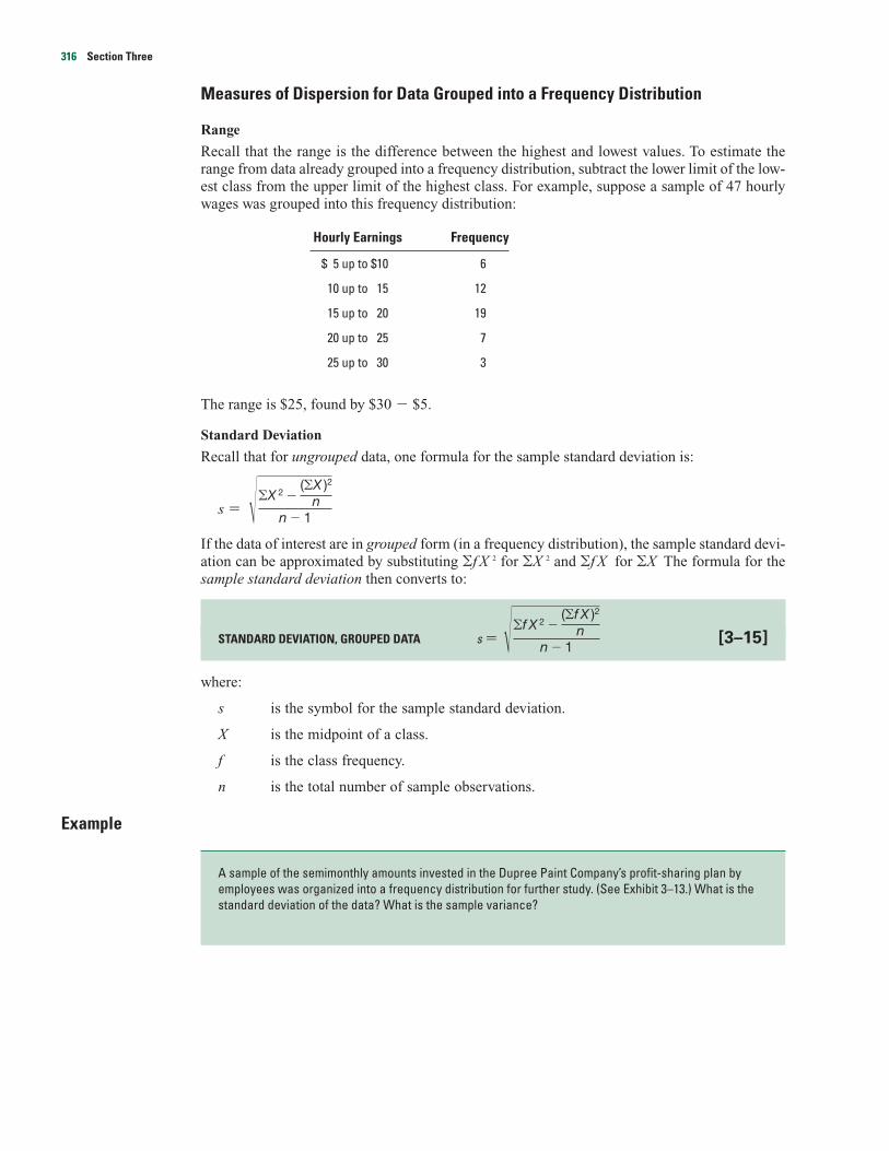
Measures of Dispersion for Data Grouped into a Frequency Distribution
Range
Recall that the range is the difference between the highest and lowest values. To estimate therange from data already grouped into a frequency distribution, subtract the lower limit of the low-est class from the upper limit of the highest class. For example, suppose a sample of 47 hourlywages was grouped into this frequency distribution:
Hourly Earnings Frequency
$ 5 up to $10 6
10 up to 15 12
15 up to 20 19
20 up to 25 7
25 up to 30 3
The range is $25, found by $30 � $5.
Standard Deviation
Recall that for ungrouped data, one formula for the sample standard deviation is:
s �
If the data of interest are in grouped form (in a frequency distribution), the sample standard devi-ation can be approximated by substituting �f X 2 for �X 2 and �f X for �X The formula for thesample standard deviation then converts to:
STANDARD DEVIATION, GROUPED DATA s � [3–15]
where:
s is the symbol for the sample standard deviation.
X is the midpoint of a class.
f is the class frequency.
n is the total number of sample observations.
Example
A sample of the semimonthly amounts invested in the Dupree Paint Company’s profit-sharing plan byemployees was organized into a frequency distribution for further study. (See Exhibit 3–13.) What is thestandard deviation of the data? What is the sample variance?
��f X 2 �(�f X )2
nn � 1
��X 2 �(�X )2
nn � 1
316 Section Three

Solution
Following the same practice used earlier for computing the arithmetic mean of data grouped into a fre-quency distribution, X represents the midpoint of each class. For example, the midpoint of the “$30 up to$35” class is $32.50. (See Exhibit 3–14.) It is assumed that the amounts invested in the “$30 up to $35”class average about $32.50. Similarly, the seven amounts in the “$35 up to $40” class are assumed toaverage about $37.50, and so on.
EXHIBIT 3–14 Calculations Needed for the Sample Standard Deviation
Amount Number, Midpoint, f X � X orInvested f X f X f X 2
$30 up to $35 3 $32.50 $ 97.50 3,168.75
35 up to 40 7 37.50 262.50 9,843.75
40 up to 45 11 42.50 467.50 19,868.75
45 up to 50 22 47.50 1,045.00 49,637.50
50 up to 55 40 52.50 2,100.00 110,250.00
55 up to 60 24 57.50 1,380.00 79,350.00
60 up to 65 9 62.50 562.50 35,156.25
65 up to 70 4 67.50 270.00 18,225.00
Total 120 $6,185.00 325,500.00
To find the standard deviation of these data grouped into a frequency distribution:
STEP 1: Each class frequency is multiplied by its class midpoint. That is, multiply f times X. Thus, for thefirst class 3 � $32.50 � $97.50, for the second class f X � 7 � $37.50 � $262.50, and so on.
STEP 2: Calculate f X 2. This could be written f X � X. For the first class it would be $97.50 � $32.50 �3,168.75, for the second class $262.50 � $37.50 � 9,843.75, and so on.
STEP 3: Sum the f X and the f X 2 columns. The totals are $6,185 and 325,500, respectively.
EXHIBIT 3–13 A Sample of Semimonthly Amounts Invested by Employees in the
Profit-Sharing Plan
Amount Number ofInvested Employees
$30 up to $35 3
35 up to 40 7
40 up to 45 11
45 up to 50 22
50 up to 55 40
55 up to 60 24
60 up to 65 9
65 up to 70 4
Introduction to Descriptive Statistics and Discrete Probability Distributions 317

Inserting these sums in formula (3–15) and solving for the sample standard deviation:
s � � � $7.51
The sample standard deviation is $7.51. The sample variance is ($7.51)2, or about 56.40 (in dollarssquared).
Self-Review 3–11
Exercises
For exercises 91–94 compute the range, the standard deviation, and the variance.
91. Refer to the following frequency distribution.
Class Frequency
0 up to 5 2
5 up to 10 7
10 up to 15 12
15 up to 20 6
20 up to 25 3
The ages of a sample of quarter-inch drills available for rental at Tool Rental, Inc. were organized into thefollowing frequency distribution.
Age (months) Frequency
2 up to 4 2
4 up to 6 5
6 up to 8 10
8 up to 10 4
10 up to 12 2
(a) Estimate the range.
(b) Estimate the sample standard deviation.
(c) Estimate the sample variance.
�325,500 � 318,785.2119
��f X 2 �(�f X )2
nn � 1
318 Section Three

92. Refer to the following frequency distribution.
Class Frequency
20 up to 30 7
30 up to 40 12
40 up to 50 21
50 up to 60 18
60 up to 70 12
93. Each person who applies for an assembly job at Carolina Furniture, Inc. is given a mechanical apti-tude test. One part of the test involves assembling a dresser based on numbered instructions. A sam-ple of the lengths of time it took 42 persons to assemble the dresser was organized into thefollowing frequency distribution.
Length of Time(minutes) Frequency
2 up to 4 4
4 up to 6 8
6 up to 8 14
8 up to 10 9
10 up to 12 5
12 up to 14 2
94. A sample of the amounts paid for parking on Saturday at the Downtown Parking Garage in Torontowas organized into the following frequency distribution.
Amount Paid Frequency
$0.50 up to $0.75 2
0.75 up to 1.00 7
1.00 up to 1.25 15
1.25 up to 1.50 28
1.50 up to 1.75 14
1.75 up to 2.00 9
2.00 up to 2.25 3
2.25 up to 2.50 2
Snapshot 3–4Todd Helton of the Colorado Rockies and Nomar Garciaparra of the Boston Red Sox tied for the highest batting average during the 2000 Major LeagueBaseball season. Each had a batting average of .372. The highest batting average in recent times was by Tony Gwynn, .394 in 1994, but this was duringa strike-shortened season. Ted Williams batted .406 in 1941, and nobody has hit over .400 since. It is interesting to note that the mean batting averagefor all players has remained constant at about .260 for more than 100 years. The standard deviation of that average, however, has declined from .049to .031. This indicates that there is less dispersion in the batting averages today and helps explain the lack of any .400 hitters in recent times.
Introduction to Descriptive Statistics and Discrete Probability Distributions 319
Interpretation and Uses of the Standard DeviationThe standard deviation is commonly used as a measure to compare the spread in two or more setsof observations. For example, the standard deviation of the semimonthly amounts invested in theDupree Paint Company profit-sharing plan was just computed to be $7.51. Suppose theseemployees are located in Georgia. If the standard deviation for a group of employees in Texas is$10.47, and the means are about the same, it indicates that the amounts invested by the Georgiaemployees are not dispersed as much as those in Texas (because $7.51 � $10.47). Since theamounts invested by the Georgia employees are clustered more closely about the mean, the meanfor the Georgia employees is a more reliable measure than the mean for the Texas group.
Chebyshev’s Theorem
We have stressed that a small standard deviation for a set of values indicates that these values arelocated close to the mean. Conversely, a large standard deviation reveals that the observations arewidely scattered about the mean. The Russian mathematician P. L. Chebyshev (1821–1894)developed a theorem that allows us to determine the minimum proportion of the values that liewithin a specified number of standard deviations of the mean. For example, based on Cheby-shev’s theorem, at least three of four values, or 75 percent, must lie between the mean plus twostandard deviations and the mean minus two standard deviations. This relationship appliesregardless of the shape of the distribution. Further, at least eight of nine values, or 88.9 percent,will lie between plus three standard deviations and minus three standard deviations of the mean.At least 24 of 25 values, or 96 percent, will lie between plus and minus five standard deviationsof the mean.
Chebyshev’s theorem states:
Example
Solution
About 92 percent, found by
1 � � 1 � � 1 � � 0.92
Snaphot 3–5Previously, we found that the average is a value used to represent all the data. However, often an average does not give the full picture. Stockbro-kers are often faced with this problem when they are considering two investments, where the mean rate of return is the same. They usually calcu-late the standard deviation of the rates of return to assess the risk associated with the two investments. The investment with the larger standarddeviation is considered to have the greater risk. In this context the standard deviation plays a vital part in making critical decisions regarding the com-position of an investor’s portfolio.
112.25
1(3.5)2
1k2
In the previous example and solution, the arithmetic mean semimonthly amount contributed by theDupree Paint employees to the company’s profit-sharing plan was $51.54, and the standard deviation wascomputed to be $7.51. At least what percent of the contributions lie within plus 3.5 standard deviationsand minus 3.5 standard deviations of the mean?
CHEBYSHEV’S THEOREM For any set of observations (sample or population), the proportion of the values thatlie within k standard deviations of the mean is at least 1 � 1/k 2, where k is any constant greater than 1.
320 Section Three
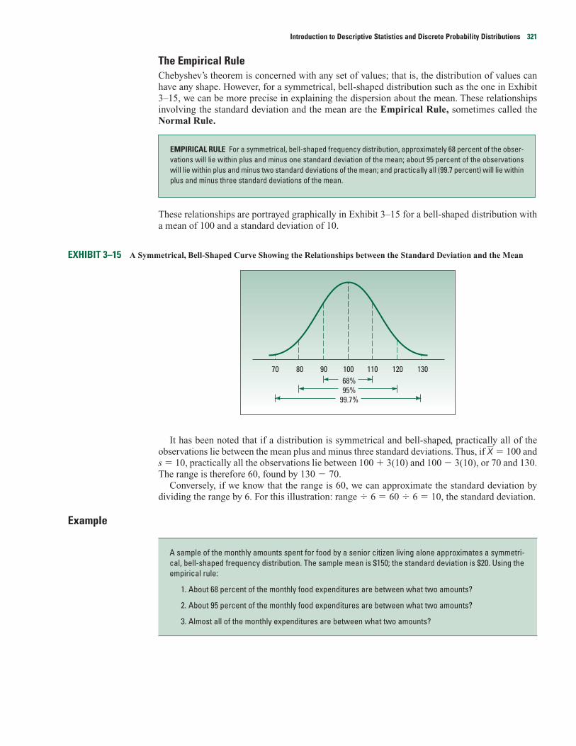
The Empirical RuleChebyshev’s theorem is concerned with any set of values; that is, the distribution of values canhave any shape. However, for a symmetrical, bell-shaped distribution such as the one in Exhibit3–15, we can be more precise in explaining the dispersion about the mean. These relationshipsinvolving the standard deviation and the mean are the Empirical Rule, sometimes called theNormal Rule.
These relationships are portrayed graphically in Exhibit 3–15 for a bell-shaped distribution witha mean of 100 and a standard deviation of 10.
EXHIBIT 3–15 A Symmetrical, Bell-Shaped Curve Showing the Relationships between the Standard Deviation and the Mean
It has been noted that if a distribution is symmetrical and bell-shaped, practically all of theobservations lie between the mean plus and minus three standard deviations. Thus, if � 100 ands � 10, practically all the observations lie between 100 � 3(10) and 100 � 3(10), or 70 and 130.The range is therefore 60, found by 130 � 70.
Conversely, if we know that the range is 60, we can approximate the standard deviation bydividing the range by 6. For this illustration: range � 6 � 60 � 6 � 10, the standard deviation.
Example
A sample of the monthly amounts spent for food by a senior citizen living alone approximates a symmetri-cal, bell-shaped frequency distribution. The sample mean is $150; the standard deviation is $20. Using theempirical rule:
1. About 68 percent of the monthly food expenditures are between what two amounts?
2. About 95 percent of the monthly food expenditures are between what two amounts?
3. Almost all of the monthly expenditures are between what two amounts?
X
908070 110 120 13010068% 95%
99.7%
EMPIRICAL RULE For a symmetrical, bell-shaped frequency distribution, approximately 68 percent of the obser-vations will lie within plus and minus one standard deviation of the mean; about 95 percent of the observationswill lie within plus and minus two standard deviations of the mean; and practically all (99.7 percent) will lie withinplus and minus three standard deviations of the mean.
Introduction to Descriptive Statistics and Discrete Probability Distributions 321
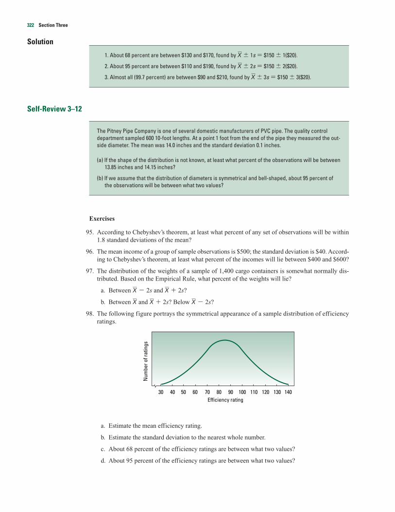
Solution
1. About 68 percent are between $130 and $170, found by 1s � $150 1($20).
2. About 95 percent are between $110 and $190, found by 2s � $150 2($20).
3. Almost all (99.7 percent) are between $90 and $210, found by 3s � $150 3($20).
Self-Review 3–12
Exercises
95. According to Chebyshev’s theorem, at least what percent of any set of observations will be within1.8 standard deviations of the mean?
96. The mean income of a group of sample observations is $500; the standard deviation is $40. Accord-ing to Chebyshev’s theorem, at least what percent of the incomes will lie between $400 and $600?
97. The distribution of the weights of a sample of 1,400 cargo containers is somewhat normally dis-tributed. Based on the Empirical Rule, what percent of the weights will lie?
a. Between � 2s and � 2s?
b. Between and � 2s? Below � 2s?
98. The following figure portrays the symmetrical appearance of a sample distribution of efficiencyratings.
a. Estimate the mean efficiency rating.
b. Estimate the standard deviation to the nearest whole number.
c. About 68 percent of the efficiency ratings are between what two values?
d. About 95 percent of the efficiency ratings are between what two values?
Efficiency rating
Num
ber o
f rat
ings
30 40 50 60 70 80 90 100 110 120 130 140
XXX
XX
The Pitney Pipe Company is one of several domestic manufacturers of PVC pipe. The quality controldepartment sampled 600 10-foot lengths. At a point 1 foot from the end of the pipe they measured the out-side diameter. The mean was 14.0 inches and the standard deviation 0.1 inches.
(a) If the shape of the distribution is not known, at least what percent of the observations will be between13.85 inches and 14.15 inches?
(b) If we assume that the distribution of diameters is symmetrical and bell-shaped, about 95 percent ofthe observations will be between what two values?
X
X
X
322 Section Three
Relative Dispersion
Coefficient of Variation
A direct comparison of two or more measures of dispersion—say, the standard deviation for adistribution of annual incomes and the standard deviation of a distribution of absenteeism for thissame group of employees—is impossible. Can we say that the standard deviation of $1,200 forthe income distribution is greater than the standard deviation of 4.5 days for the distribution ofabsenteeism? Obviously not, because we cannot directly compare dollars and days absent fromwork. In order to make a meaningful comparison of the dispersion in incomes and absenteeism,we need to convert each of these measures to a relative value—that is, a percent. Karl Pearson(1857–1936), who contributed significantly to the science of statistics, developed a relative mea-sure called the coefficient of variation (CV). It is a very useful measure when:
1. The data are in different units (such as dollars and days absent).
2. The data are in the same units, but the means are far apart (such as the incomes of the top execu-tives and the incomes of the unskilled employees).
In terms of a formula for a sample:
COEFFICIENT OF VARIATION CV � (100) ←→ [3–16]
Example
Solution
The distributions are in different units (dollars and years of service). Therefore, they are converted tocoefficients of variation.
For the bonus paid: For years of service:
CV � (100) CV � (100)
� (100) � (100)
� 20 percent � 10 percent
Interpreting, there is more dispersion relative to the mean in the distribution of bonus paid comparedwith the distribution of years of service (because 20 percent 10 percent).
220
$40200
sX
sX
A study of the amount of bonus paid and the years of service of employee resulted in these statistics: Themean bonus paid was $200; the standard deviation was 40. The mean number of years of service was 20years; the standard deviation was 2 years. Compare the relative dispersion in the two distributions usingthe coefficient of variation.
Multiplying by 100converts the decimalto a percent
sX
COEFFICIENT OF VARIATION The ratio of the standard deviation to the arithmetic mean, expressed as a percent.
Introduction to Descriptive Statistics and Discrete Probability Distributions 323
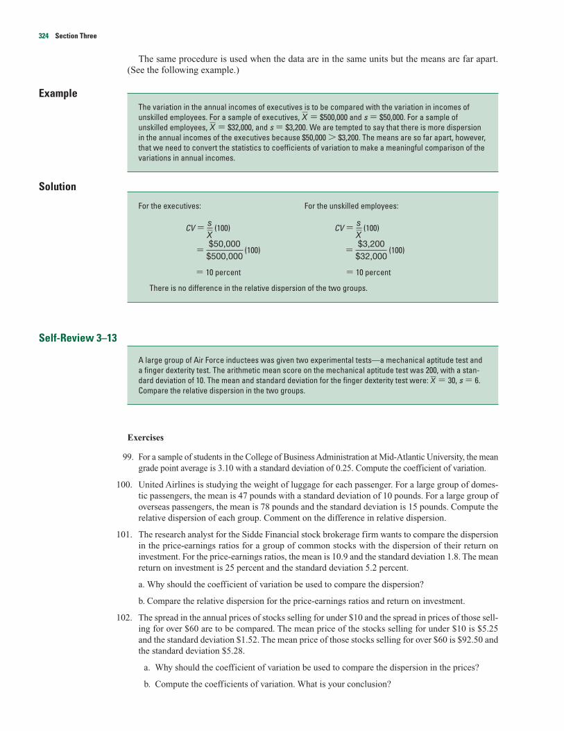
The same procedure is used when the data are in the same units but the means are far apart.(See the following example.)
ExampleThe variation in the annual incomes of executives is to be compared with the variation in incomes ofunskilled employees. For a sample of executives, � $500,000 and s � $50,000. For a sample ofunskilled employees, � $32,000, and s � $3,200. We are tempted to say that there is more dispersionin the annual incomes of the executives because $50,000 $3,200. The means are so far apart, however,that we need to convert the statistics to coefficients of variation to make a meaningful comparison of thevariations in annual incomes.
Solution
For the executives: For the unskilled employees:
CV � (100) CV � (100)
� (100) � (100)
� 10 percent � 10 percent
There is no difference in the relative dispersion of the two groups.
Self-Review 3–13
A large group of Air Force inductees was given two experimental tests—a mechanical aptitude test anda finger dexterity test. The arithmetic mean score on the mechanical aptitude test was 200, with a stan-dard deviation of 10. The mean and standard deviation for the finger dexterity test were: � 30, s � 6.Compare the relative dispersion in the two groups.
Exercises
99. For a sample of students in the College of Business Administration at Mid-Atlantic University, the meangrade point average is 3.10 with a standard deviation of 0.25. Compute the coefficient of variation.
100. United Airlines is studying the weight of luggage for each passenger. For a large group of domes-tic passengers, the mean is 47 pounds with a standard deviation of 10 pounds. For a large group ofoverseas passengers, the mean is 78 pounds and the standard deviation is 15 pounds. Compute therelative dispersion of each group. Comment on the difference in relative dispersion.
101. The research analyst for the Sidde Financial stock brokerage firm wants to compare the dispersionin the price-earnings ratios for a group of common stocks with the dispersion of their return oninvestment. For the price-earnings ratios, the mean is 10.9 and the standard deviation 1.8. The meanreturn on investment is 25 percent and the standard deviation 5.2 percent.
a. Why should the coefficient of variation be used to compare the dispersion?
b. Compare the relative dispersion for the price-earnings ratios and return on investment.
102. The spread in the annual prices of stocks selling for under $10 and the spread in prices of those sell-ing for over $60 are to be compared. The mean price of the stocks selling for under $10 is $5.25and the standard deviation $1.52. The mean price of those stocks selling for over $60 is $92.50 andthe standard deviation $5.28.
a. Why should the coefficient of variation be used to compare the dispersion in the prices?
b. Compute the coefficients of variation. What is your conclusion?
X
$3,200$32,000
$50,000$500,000
sX
sX
XX
324 Section Three
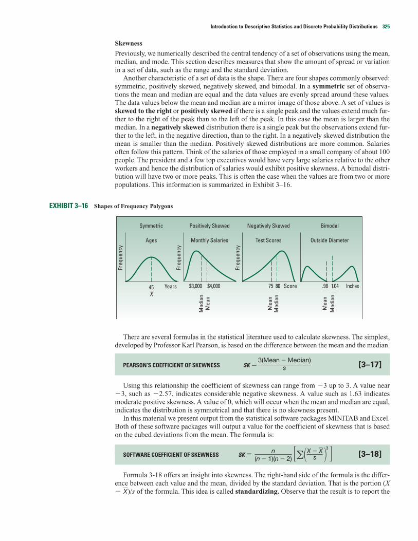
Skewness
Previously, we numerically described the central tendency of a set of observations using the mean,median, and mode. This section describes measures that show the amount of spread or variationin a set of data, such as the range and the standard deviation.
Another characteristic of a set of data is the shape. There are four shapes commonly observed:symmetric, positively skewed, negatively skewed, and bimodal. In a symmetric set of observa-tions the mean and median are equal and the data values are evenly spread around these values.The data values below the mean and median are a mirror image of those above. A set of values isskewed to the right or positively skewed if there is a single peak and the values extend much fur-ther to the right of the peak than to the left of the peak. In this case the mean is larger than themedian. In a negatively skewed distribution there is a single peak but the observations extend fur-ther to the left, in the negative direction, than to the right. In a negatively skewed distribution themean is smaller than the median. Positively skewed distributions are more common. Salariesoften follow this pattern. Think of the salaries of those employed in a small company of about 100people. The president and a few top executives would have very large salaries relative to the otherworkers and hence the distribution of salaries would exhibit positive skewness. A bimodal distri-bution will have two or more peaks. This is often the case when the values are from two or morepopulations. This information is summarized in Exhibit 3–16.
EXHIBIT 3–16 Shapes of Frequency Polygons
There are several formulas in the statistical literature used to calculate skewness. The simplest,developed by Professor Karl Pearson, is based on the difference between the mean and the median.
PEARSON’S COEFFICIENT OF SKEWNESS SK � [3–17]
Using this relationship the coefficient of skewness can range from �3 up to 3. A value near�3, such as �2.57, indicates considerable negative skewness. A value such as 1.63 indicatesmoderate positive skewness. A value of 0, which will occur when the mean and median are equal,indicates the distribution is symmetrical and that there is no skewness present.
In this material we present output from the statistical software packages MINITAB and Excel.Both of these software packages will output a value for the coefficient of skewness that is basedon the cubed deviations from the mean. The formula is:
SOFTWARE COEFFICIENT OF SKEWNESS SK � [3–18]
Formula 3-18 offers an insight into skewness. The right-hand side of the formula is the differ-ence between each value and the mean, divided by the standard deviation. That is the portion (X� )/s of the formula. This idea is called standardizing. Observe that the result is to report theX
���X � Xs �
3
n(n � 1)(n � 2)
3(Mean � Median)s
Med
ian
Mea
n
45X
Freq
uenc
y
Years
Ages
Symmetric
Freq
uenc
y
Monthly Salaries
Positively Skewed
$3,000 $4,000
Med
ian
Mea
n
Freq
uenc
yTest Scores
Negatively Skewed
75 80 Score
Med
ian
Mea
n
Outside Diameter
Bimodal
.98 1.04 Inches
Introduction to Descriptive Statistics and Discrete Probability Distributions 325

difference between each value and the mean in units of the standard deviation. If this differenceis positive, the particular value is larger than the mean; if it is negative, it is smaller than the mean.When we cube these values, we retain the information on the direction of the difference. Recallthat in the formula for the standard deviation (see formula 3–14) we squared the differencebetween each value and the mean, so that result was all positive values.
If the set of data values under consideration is symmetric, when we cube the standardized val-ues and sum over all the values the result would be near zero. If there are several large values,clearly separate from the others, the sum of the cubed differences would be a large positive value.Several values much smaller will result in a negative cubed sum.
An example will illustrate the idea of skewness.
Example
Solution
These are ungrouped sample data, so we use formula 3–2 to determine the mean
� � � $4.95
The median is the middle value in a set of data, arranged from smallest to largest. In this case themiddle value is $3.18, so the median earnings per share is $3.18.
We use formula 3–14 to determine the sample standard deviation.
s � � 5.22
Pearson’s coefficient of skewness is 1.017, found by
sk � � � 1.017
This indicates there is moderate positive skewness in the earnings per share data.
We obtain a similar, but not exactly the same, value from the software method. The details of the calcu-lations are shown in Exhibit 3–17. To begin we find the difference between each earnings per share valueand the mean and divide this result by the standard deviation. Recall that we referred to this as standard-izing. Next, we cube, that is, raise it to the third power, the result of the first step. Finally, we sum thecubed values. The details of the first row, that is, the company with an earnings per share of $0.09, are:
� � (�0.9310)3 � �0.8070�0.09 � 4.955.22 �
3
�X � Xs �
3
3($4.95 � $3.18)
$5.22
3(Mean � Median)s
�749.372 �(74.26)2
1515 � 1
��X 2 �(�X )
nn � 1
$74.2615
�XnX
Following are the earning per share for a sample of 15 software companies for the year 2000. The earn-ings per share are arranged from smallest to largest.
$0.09 $0.13 $0.41 $0.51 $ 1.12 $ 1.20 $ 1.49 $3.18
3.50 6.36 7.83 8.92 10.13 12.99 16.40
Compute the mean, median, and standard deviation. Find the coefficient of skewness using Pearson’sestimate and the software methods. What is your conclusion regarding the shape of the distribution?
326 Section Three

When we sum the 15 cubed values the result is 11.8274. That is, the term �[(X � )/s]3 � 11.8274. Tofind the coefficient of skewness, we use formula 3–18, with n � 15.
sk � � (11.8274) � 0.975
EXHIBIT 3–17 Calculation of the Coefficient of Skewness.
Earnings per Share
0.09 �0.9310 �0.8070
0.13 �0.9234 �0.7873
0.41 �0.8697 �0.6579
0.51 �0.8506 �0.6154
1.12 �0.7337 �0.3950
1.20 �0.7184 �0.3708
1.49 �0.6628 �0.2912
3.18 �0.3391 �0.0390
3.50 �0.2778 �0.0214
6.36 0.2701 0.0197
7.83 0.5517 0.1679
8.92 0.7605 0.4399
10.13 0.9923 0.9772
12.99 1.5402 3.6539
16.40 2.1935 10.5537
11.8274
We conclude that the earnings per share values are somewhat positively skewed. The followingchart, from MINITAB, reports the descriptive measures, such as the mean, median, and standard devia-tion of the earnings per share data. Also included are the coefficient of skewness and a histogram with abell-shaped curve superimposed.
�X � Xs �
3(X � X )s
15(15 � 1)(15 � 2)��X � X
s �3n
(n � 1)(n � 2)
X
Introduction to Descriptive Statistics and Discrete Probability Distributions 327
Self-Review 3–14
Exercises
For exercises 103–106, do the following:
a. Determine the mean, median, and the standard deviation.
b. Determine the coefficient of skewness using Pearson’s method.
c. Determine the coefficient of skewness using the software method.
103. The following values are the starting salaries, in $000, for a sample of five accounting graduateswho accepted positions in public accounting last year.
36.0 26.0 33.0 28.0 31.0
104. Listed below are the salaries, in $000, for a sample of 15 executives in the electronics industry.
$516.0 $548.0 $566.0 $534.0 $586.0 $529.0
546.0 523.0 538.0 523.0 551.0 552.0
486.0 558.0 574.0
105. Listed below are the commissions earned ($000) last year by the sales representatives at the Fur-niture Patch.
$ 3.9 $ 5.7 $ 7.3 $10.6 $13.0 $13.6 $15.1 $15.8 $17.1
17.4 17.6 22.3 38.6 43.2 87.7
106. Listed below are the salaries for the New York Yankees for the year 2000. The salary informationis reported in millions of dollars.
$9.86 $9.50 $8.25 $6.25 $6.00 $5.95
5.25 5.00 4.33 4.30 4.25 3.40
3.13 2.02 2.00 1.90 1.85 1.82
0.80 0.38 0.35 0.35 0.20 0.20
0.20 0.20 0.20 0.20 0.20
Other Measures of DispersionThe standard deviation is the most widely used measure of dispersion. However, there are otherways of describing the variation or spread in a set of data. One method is to determine the loca-tion of values that divide a set of observations into equal parts. These measures include quartiles,deciles, and percentiles.
Quartiles divide a set of observations into four equal parts. To explain further, think of any setof values arranged from smallest to largest. We called the middle value of a set of data arrangedfrom smallest to largest the median. That is, 50 percent of the observations are larger than themedian and 50 percent are smaller. The median is a measure of location because it pinpoints the
A sample of 5 data entry clerks employed in the Horry County Tax Office revised the following number oftax records last hour: 73, 98, 60, 92, and 84.
(a) Find the mean, median, and the standard deviation.
(b) Compute the coefficient of skewness using Pearson’s method.
(c) Calculate the coefficient of skewness using the software method.
(d) What is your conclusion regarding the skewness of the data?
328 Section Three

center of the data. In a similar fashion quartiles divide a set of observations into four equal parts.The first quartile, usually labeled Q1, is the value below which 25 percent of the observationsoccur and the third quartile, usually labeled Q3, is the value below which 75 percent of the obser-vations occur. Logically, Q2 is the median. The values corresponding to Q1, Q2, and Q3 divide a setof data into four equal parts. Q1 can be thought of as the “median” of the lower half of the dataand Q3 the “median” of the upper half of the data.
In a similar fashion deciles divide a set of observations into 10 equal parts and percentiles into100 equal parts. So if you found that your GPA was in the 8th decile at your university, you couldconclude that 80 percent of the students had a GPA lower than yours and 20 percent had a higherGPA. A GPA in the 33rd percentile means that 33 percent of the students have a lower GPA and67 percent have a higher GPA. Percentile scores are frequently used to report results on suchnational standardized tests as the SAT, ACT, GMAT (used to judge entry into many Master ofBusiness Administration programs), and LSAT (used to judge entry into law school).
Quartiles, Deciles, and Percentiles
To formalize the computational procedure, let Lp refer to the location of a desired percentile. Soif we wanted to find the 33rd percentile we would use L33 and if we wanted the median, the 50thpercentile, then L50. The number of observations is n, so if we want to locate the middle observa-tion, its position is at (n � 1)/2, or we could write this as (n � 1)(P/100), where P is the desiredpercentile.
LOCATION OF A PERCENTILE Lp � (n � 1) [3–19]
An example will help to explain further.
Example
Solution
The first step is to organize the data from the smallest commission to the largest.
$1,460 $1,471 $1,637 $1,721 $1,758 $1,787 $1,940 $2,038
2,047 2,054 2,097 2,205 2,287 2,311 2,406
The median value is the observation in the center. The center value or L50 is located at (n � 1)/2,where n is the number of observations. In this case that is position number 8, found by (15 � 1)/2. Theeighth largest commission is $2,038. So we conclude this is the median and that half the brokers earnedcommissions more than $2,038 and half earned less than $2,038.
Listed below are the commissions earned last month by a sample of 15 brokers at Salomon Smith Bar-ney’s Oakland, California, office. Salomon Smith Barney is an investment company with offices locatedthroughout the United States.
$2,038 $1,758 $1,721 $1,637 $2,097 $2,047 $2,205 $1,787 $2,287
1,940 2,311 2,054 2,406 1,471 1,460
Locate the median, the first quartile, and the third quartile for the commissions earned.
P100
Introduction to Descriptive Statistics and Discrete Probability Distributions 329
Recall the definition of a quartile. Quartiles divide a set of observations into four equal parts. Hence 25 percent of the observations will be less than the first quartile. Seventy-five percent of the observationswill be less than the third quartile. To locate the first quartile, we use formula (3–19), where n � 15 and P � 25:
L25 � (n � 1) � (15 � 1) � 4
and to locate the third quartile, n � 15 and P � 75:
L75 � (n � 1) � (15 � 1) � 12
Therefore, the first and third quartile values are located at positions 4 and 12. The fourth value in theordered array is $1,721 and the twelfth is $2,205. These are the first and third quartiles, respectively.
In the above example the location formula yielded a whole number result. That is, we werelooking to find the first quartile and there were 15 observations, so the location formula indi-cated we should look to the fourth ordered value. What if there were 20 observations in the sam-ple, that is n � 20, and we wanted to locate the first quartile? From the location formula (3–19):
L25 � (n � 1) � (20 � 1) � 5.25
We would locate the fifth value in the ordered array and then move .25 of the distance betweenthe 5th and 6th values and report that as the first quartile. Like the median, the quartile does notneed to be one of the actual values in the data set.
To explain further, suppose a data set contained the six values: 91, 75, 61, 101, 43, and 104.We want to locate the first quartile. We order the values from smallest to largest: 43, 61, 75, 91,101, and 104. The first quartile is located at
L25 � (n � 1) � (6 � 1) � 1.75
The position formula tells us that the first quartile is located between the first and the secondvalue and that it is .75 of the distance between the first and the second values. The first value is43 and the second is 61. So the distance between these two values is 18. To locate the first quar-tile, we need to move .75 of the distance between the first and second values, so .75(18) � 13.5.To complete the procedure, we add 13.5 to the first value and report that the first quartile islocated at 56.5.
We can extend the idea to include both deciles and percentiles. If we wanted to locate the 23rdpercentile in a sample of 80 observations, we would look for the 18.63 position.
L23 � (n � 1) � (80 � 1) � 18.63
To find the value corresponding to the 23rd percentile, we would locate the 18th value and the19th value and determine the distance between the two values. Next, we would multiply this dif-ference by 0.63 and add the result to the smaller value. The result would be the 23rd percentile.
With a computer software package, it is quite easy to sort the data from smallest to largest andto locate percentiles and deciles. Both MINITAB and Excel output summary statistics. Listed
23100
P100
25100
P100
25100
P100
75100
P100
25100
P100
330 Section Three

below is the MINITAB output. It includes the first and third quartiles, as well as the mean,median, standard deviation, and coefficient of skewness for the Whitner Pontiac data (seeExhibit 3–2). We conclude that 25 percent of the vehicles sold for less than $17,074 and that 75percent sold for less than $22,795.
The Excel output following includes the same information regarding the mean, median, standarddeviation, and coefficient of skewness. It will also output the quartiles, but the method of calcula-tion is not as precise. To find the quartiles, we multiply the sample size by the desired percentile andreport the integer of that value. To explain, in the Whitner Pontiac data there are 80 observations, andwe wish to locate the 25th percentile. We multiply 80 by .25; the result is 20.25. Excel will not allowus to enter a fractional value, so we use 20 and request the location of the largest 20 values and thesmallest 20 values. The result is a good approximation of the 25th and 75th percentiles.
Introduction to Descriptive Statistics and Discrete Probability Distributions 331

Self-Review 3–15
Exercises
107. Determine the median and the values corresponding to the first and third quartiles in thefollowing data.
46 47 49 49 51 53 54 54 55 55 59
108. Determine the median and the values corresponding to the first and third quartiles in thefollowing data.
5.24 6.02 6.67 7.30 7.59 7.99 8.03 8.35 8.81 9.45
9.61 10.37 10.39 11.86 12.22 12.71 13.07 13.59 13.89 15.42
109. Anderson, Inc., is a distributor of small electrical motors. As with any business, the length of timecustomers take to pay their invoices is important. Listed below, arranged from smallest to largest,is the time, in days, for a sample of Anderson, Inc., invoices.
13 13 13 20 26 27 31 34 34 34 35 35 36 37 38
41 41 41 45 47 47 47 50 51 53 54 56 62 67 82
a. Determine the first and third quartiles.
b. Determine the 2nd decile and the 8th decile.
c. Determine the 67th percentile.
110. Wendy Hagel is the national sales manager for National Textbooks, Inc. She has a sales staff of 40who visit college professors all over the United States. Each Saturday morning she requires hersales staff to send her a report. This report includes, among other things, the number of professorsvisited during the previous week. Listed below, ordered from smallest to largest, are the number ofvisits last week.
38 40 41 45 48 48 50 50 51 51 52 52 53 54 55 55 55 56 56 57
59 59 59 62 62 62 63 64 65 66 66 67 67 69 69 71 77 78 79 79
a. Determine the median number of calls.
b. Determine the first and third quartiles.
c. Determine the 1st decile and the 9th decile.
d. Determine the 33rd percentile.
Box Plots
A box plot is a graphical display, based on quartiles, that helps us picture a set of data. To con-struct a box plot, we need only five statistics: the minimum value, Q1 (the first quartile), themedian, Q3 (the third quartile), and the maximum value. An example will help to explain.
The quality control department of the Plainsville Peanut Company is responsible for checking the weightof the 8-ounce jar of peanut butter. The weights of a sample of 9 jars produced last hour are:
7.69 7.72 7.8 7.86 7.90 7.94 7.97 8.06 8.09
(a) What is the median weight?
(b) Determine the weights corresponding to the first and third quartiles.
332 Section Three
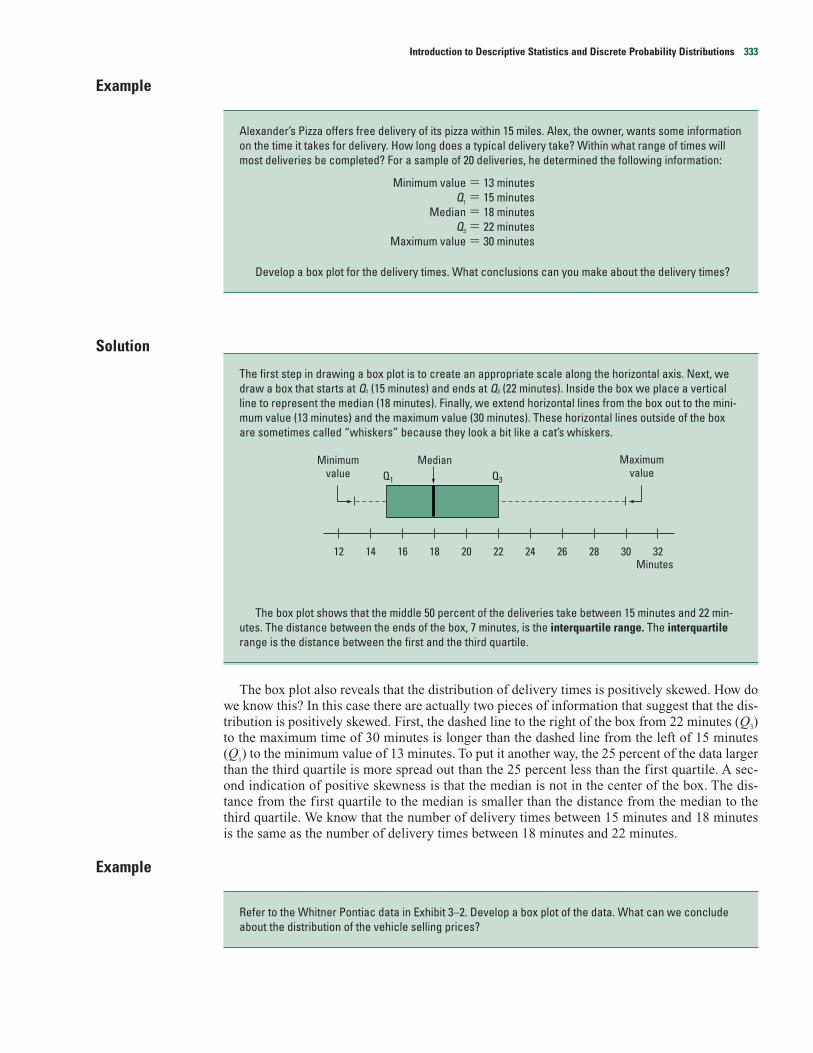
Example
Solution
The first step in drawing a box plot is to create an appropriate scale along the horizontal axis. Next, wedraw a box that starts at Q1 (15 minutes) and ends at Q3 (22 minutes). Inside the box we place a verticalline to represent the median (18 minutes). Finally, we extend horizontal lines from the box out to the mini-mum value (13 minutes) and the maximum value (30 minutes). These horizontal lines outside of the boxare sometimes called “whiskers” because they look a bit like a cat’s whiskers.
The box plot shows that the middle 50 percent of the deliveries take between 15 minutes and 22 min-utes. The distance between the ends of the box, 7 minutes, is the interquartile range. The interquartilerange is the distance between the first and the third quartile.
The box plot also reveals that the distribution of delivery times is positively skewed. How dowe know this? In this case there are actually two pieces of information that suggest that the dis-tribution is positively skewed. First, the dashed line to the right of the box from 22 minutes (Q3)to the maximum time of 30 minutes is longer than the dashed line from the left of 15 minutes(Q
1) to the minimum value of 13 minutes. To put it another way, the 25 percent of the data larger
than the third quartile is more spread out than the 25 percent less than the first quartile. A sec-ond indication of positive skewness is that the median is not in the center of the box. The dis-tance from the first quartile to the median is smaller than the distance from the median to thethird quartile. We know that the number of delivery times between 15 minutes and 18 minutesis the same as the number of delivery times between 18 minutes and 22 minutes.
Example
Refer to the Whitner Pontiac data in Exhibit 3–2. Develop a box plot of the data. What can we concludeabout the distribution of the vehicle selling prices?
12 14 16 18 20 22 24 26 28 30 32
Q1
MedianQ3
Minimumvalue
Maximumvalue
Minutes
Alexander’s Pizza offers free delivery of its pizza within 15 miles. Alex, the owner, wants some informationon the time it takes for delivery. How long does a typical delivery take? Within what range of times willmost deliveries be completed? For a sample of 20 deliveries, he determined the following information:
Minimum value � 13 minutesQ1 � 15 minutes
Median � 18 minutesQ3 � 22 minutes
Maximum value � 30 minutes
Develop a box plot for the delivery times. What conclusions can you make about the delivery times?
Introduction to Descriptive Statistics and Discrete Probability Distributions 333

Solution
The MINITAB statistical software system was used to develop the following chart.
We conclude that the median vehicle selling price is about $20,000, that about 25 percent of the vehi-cles sell for less than $17,000, and that about 25 percent sell for more than $23,000. About 50 percent ofthe vehicles sell for between $17,000 and $23,000. The distribution is positively skewed because the solidline above $23,000 is somewhat longer than the line below $17,000.
There is an asterisk (*) above the $30,000 selling price. An asterisk indicates an outlier. An outlier is avalue that is inconsistent with the rest of the data. The standard definition of an outlier is a value that ismore than 1.5 times the interquartile range smaller than Q1 or larger than Q3. In this example, an outlierwould be a value larger than $32,000, found by
Outlier Q3 � 1.5(Q3 � Q1) � $23,000 � 1.5($23,000 � $17,000) � $32,000
A value less than $8,000 is also an outlier.
Outlier Q1 � 1.5(Q3 � Q1) � $23,000 � 1.5($23,000 � $17,000) � $8,000
The MINITAB box plot indicates that there is only one value larger than $32,000. However, if you lookat the actual data in Exhibit 3–2 you will notice that there are actually two values ($32,851 and $32,925).The software was not able to graph two data points so close together, so it shows only one asterisk.
Self-Review 3–16
The following box plot is given.
What are the median, the largest and smallest values, and the first and third quartiles? Would youagree that the distribution is symmetrical?
0 10 20 30 40 50 60 70 80 90 100
334 Section Three
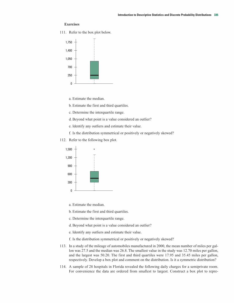
Exercises
111. Refer to the box plot below.
a. Estimate the median.
b. Estimate the first and third quartiles.
c. Determine the interquartile range.
d. Beyond what point is a value considered an outlier?
e. Identify any outliers and estimate their value.
f. Is the distribution symmetrical or positively or negatively skewed?
112. Refer to the following box plot.
a. Estimate the median.
b. Estimate the first and third quartiles.
c. Determine the interquartile range.
d. Beyond what point is a value considered an outlier?
e. Identify any outliers and estimate their value.
f. Is the distribution symmetrical or positively or negatively skewed?
113. In a study of the mileage of automobiles manufactured in 2000, the mean number of miles per gal-lon was 27.5 and the median was 26.8. The smallest value in the study was 12.70 miles per gallon,and the largest was 50.20. The first and third quartiles were 17.95 and 35.45 miles per gallon,respectively. Develop a box plot and comment on the distribution. Is it a symmetric distribution?
114. A sample of 28 hospitals in Florida revealed the following daily charges for a semiprivate room. For convenience the data are ordered from smallest to largest. Construct a box plot to repre-
1,500
1,200
900
600
300
0
*
1,750
1,400
1,050
700
350
0
Introduction to Descriptive Statistics and Discrete Probability Distributions 335
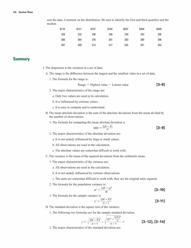
sent the data. Comment on the distribution. Be sure to identify the first and third quartiles and themedian.
$116 $121 $157 $192 $207 $209 $209
229 232 236 236 239 243 246
260 264 276 281 283 289 296
307 309 312 317 324 341 353
Summary
I. The dispersion is the variation in a set of data.
A. The range is the difference between the largest and the smallest value in a set of data.
1. The formula for the range is:
Range � Highest value � Lowest value [3–8]
2. The major characteristics of the range are:
a. Only two values are used in its calculation.
b. It is influenced by extreme values.
c. It is easy to compute and to understand.
B. The mean absolute deviation is the sum of the absolute deviations from the mean divided bythe number of observations.
1. The formula for computing the mean absolute deviation is
MD � [3–9]
2. The major characteristics of the absolute deviation are:
a. It is not unduly influenced by large or small values.
b. All observations are used in the calculation.
c. The absolute values are somewhat difficult to work with.
C. The variance is the mean of the squared deviations from the arithmetic mean.
1. The major characteristics of the variance are:
a. All observations are used in the calculation.
b. It is not unduly influenced by extreme observations.
c. The units are somewhat difficult to work with; they are the original units squared.
2. The formula for the population variance is:
�2 � [3–10]
3. The formula for the sample variance is
s2 � [3-11]
D. The standard deviation is the square root of the variance.
1. The following two formulas are for the sample standard deviation.
s � � � [3–12], [3–14]
2. The major characteristics of the standard deviation are:
��X 2 �(�X )2
nn � 1
��(X � X )2
n � 1
�(X � X )2
n � 1
�(X � �)2
N
��X � X �n
336 Section Three
a. It is in the same units as the original data.
b. It is the square root of the average squared distance from the mean.
c. It cannot be negative.
d. It is the most widely reported measure of dispersion.
II. Chebyshev’s theorem states that regardless of the shape of the distribution, at least 1 – 1/k2 of theobservations will be within k standard deviations of the mean.
III. The coefficient of variation is a measure of relative dispersion.
A. The formula for the coefficient of variation is:
CV � (100) [3–16]
B. It reports the variation relative to the mean.
C. It is useful for comparing distributions with different units.
IV. The coefficient of skewness measures the symmetry of a distribution.
A. In a positively skewed set of data the long tail is to the right.
B. In a negatively skewed distribution the long tail is to the left.
V. Measures of location also describe the spread in a set of observations.
A. A quartile divides a set of observations into four equal parts.
1. Twenty-five percent of the observations are less than the first quartile, 50 percent are lessthan the second quartile (the median), and 75 percent are less than the third quartile.
2. The interquartile range is the difference between the third and the first quartile.
B. Deciles divide a set of observations into 10 equal parts.
C. Percentiles divide a set of observations into 100 equal parts.
D. A box plot is a graphic display of a set of data.
1. A box is drawn enclosing the first and third quartiles.
a. A line through the inside of the box shows the median.
b. Dotted line segments from the third quartile to the largest value and from the first quartileto the smallest value show the range of the largest 25 percent of the observations and thesmallest 25 percent.
2. A box plot is based on five statistics: the largest and smallest observation, the first and thirdquartiles, and the median.
Pronunciation Key
SYMBOL MEANING PRONUNCIATION
�2 Population variance sigma squared
� Population standard deviation sigma
�f X2 Sum of the product of the class sigma f X squaredmidpoints squared and the classfrequency
Lp Location of percentile L sub p
Q1 First quartile Q sub 1
Q3 Third quartile Q sub 3
sX
Introduction to Descriptive Statistics and Discrete Probability Distributions 337
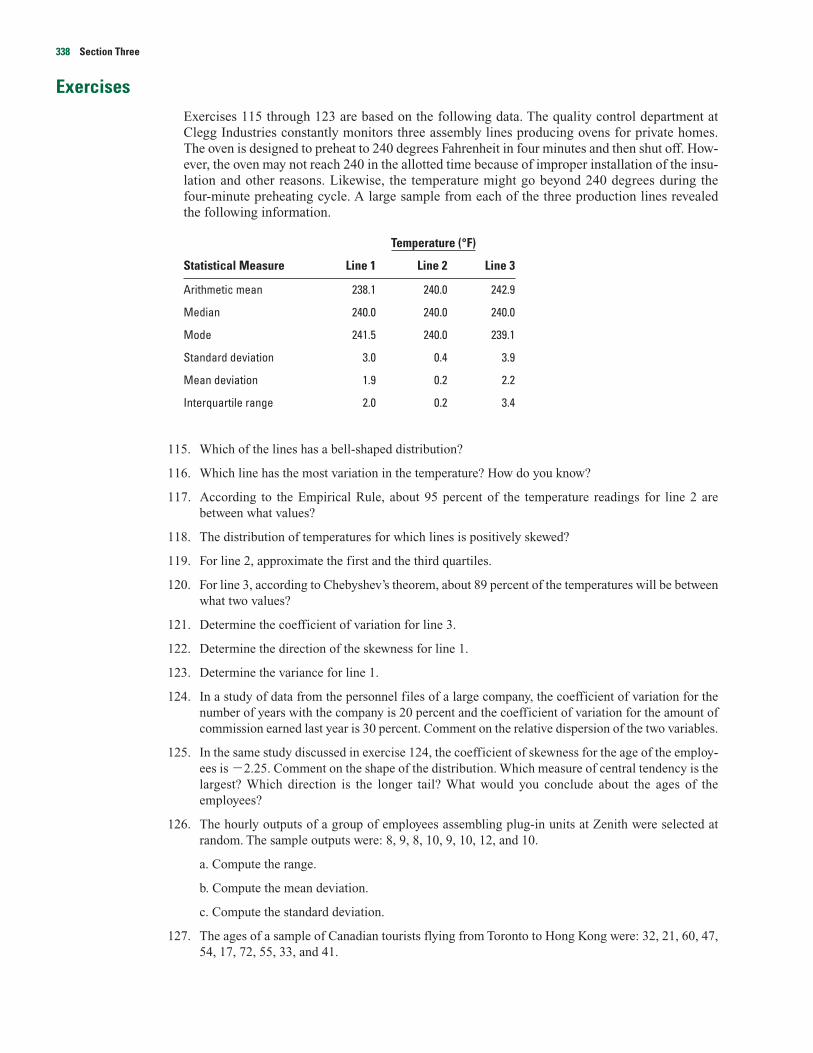
ExercisesExercises 115 through 123 are based on the following data. The quality control department atClegg Industries constantly monitors three assembly lines producing ovens for private homes.The oven is designed to preheat to 240 degrees Fahrenheit in four minutes and then shut off. How-ever, the oven may not reach 240 in the allotted time because of improper installation of the insu-lation and other reasons. Likewise, the temperature might go beyond 240 degrees during thefour-minute preheating cycle. A large sample from each of the three production lines revealedthe following information.
Temperature (°F)
Statistical Measure Line 1 Line 2 Line 3
Arithmetic mean 238.1 240.0 242.9
Median 240.0 240.0 240.0
Mode 241.5 240.0 239.1
Standard deviation 3.0 0.4 3.9
Mean deviation 1.9 0.2 2.2
Interquartile range 2.0 0.2 3.4
115. Which of the lines has a bell-shaped distribution?
116. Which line has the most variation in the temperature? How do you know?
117. According to the Empirical Rule, about 95 percent of the temperature readings for line 2 arebetween what values?
118. The distribution of temperatures for which lines is positively skewed?
119. For line 2, approximate the first and the third quartiles.
120. For line 3, according to Chebyshev’s theorem, about 89 percent of the temperatures will be betweenwhat two values?
121. Determine the coefficient of variation for line 3.
122. Determine the direction of the skewness for line 1.
123. Determine the variance for line 1.
124. In a study of data from the personnel files of a large company, the coefficient of variation for thenumber of years with the company is 20 percent and the coefficient of variation for the amount ofcommission earned last year is 30 percent. Comment on the relative dispersion of the two variables.
125. In the same study discussed in exercise 124, the coefficient of skewness for the age of the employ-ees is �2.25. Comment on the shape of the distribution. Which measure of central tendency is thelargest? Which direction is the longer tail? What would you conclude about the ages of theemployees?
126. The hourly outputs of a group of employees assembling plug-in units at Zenith were selected atrandom. The sample outputs were: 8, 9, 8, 10, 9, 10, 12, and 10.
a. Compute the range.
b. Compute the mean deviation.
c. Compute the standard deviation.
127. The ages of a sample of Canadian tourists flying from Toronto to Hong Kong were: 32, 21, 60, 47,54, 17, 72, 55, 33, and 41.
338 Section Three

a. Compute the range.
b. Compute the mean deviation.
c. Compute the standard deviation.
128. The weights (in pounds) of a sample of five boxes being sent by UPS are: 12, 6, 7, 3, and 10.
a. Compute the range.
b. Compute the mean deviation.
c. Compute the standard deviation.
129. A southern state has seven state universities in its system. The numbers of volumes (in thousands)held in their libraries are 83, 510, 33, 256, 401, 47, and 23.
a. Is this a sample or a population?
b. Compute the standard deviation.
c. Compute the coefficient of variation. Interpret.
130. A recent report in Woman’s World magazine suggested that the typical family of four with an inter-mediate budget spends about $96 per week on food. The following frequency distribution wasincluded in the report. Compute (a) the range and (b) the standard deviation.
Amount Spent Frequency
$ 80 up to $ 85 6
85 up to 90 12
90 up to 95 23
95 up to 100 35
100 up to 105 24
105 up to 110 10
131. Bidwell Electronics, Inc., recently surveyed a sample of employees to determine how far they livedfrom corporate headquarters. The results are shown below. Compute the range and the standarddeviation.
Distance(miles) Frequency
0 up to 5 4
5 up to 10 15
10 up to 15 27
15 up to 20 18
20 up to 25 6
Introduction to Descriptive Statistics and Discrete Probability Distributions 339

132. Health issues are a concern of managers, especially as they evaluate the cost of medical insurance.In a recent survey of 150 executives at Elvers Industries, a large insurance and financial firmlocated in the Southwest, the number of pounds by which the executives were overweight wasreported. Compute the range and the standard deviation.
PoundsOverweight Frequency
0 up to 6 14
6 up to 12 42
12 up to 18 58
18 up to 24 28
24 up to 30 8
133. A major airline wanted some information on those enrolled in their “frequent flyer” program. Asample of 48 members resulted in the following number of miles flown, to the near-est 1,000 miles, by each participant. Develop a box plot of the data and comment on theinformation.
22 29 32 38 39 41 42 43 43 43 44 44
45 45 46 46 46 47 50 51 52 54 54 55
56 57 58 59 60 61 61 63 63 64 64 67
69 70 70 70 71 71 72 73 74 76 78 88
134. The National Muffler Company claims they will change your muffler in less than 30 minutes. Anundercover consumer reporter for WTOL Channel 11 monitored 30 consecutive muffler changes atthe National outlet on Liberty Street. The number of minutes to perform changes is reported below.
44 12 22 31 26 22 30 26 18 28 12
40 17 13 14 17 25 29 15 30 10 28
16 33 24 20 29 34 23 13
a. Develop a box plot for the time to change a muffler.
b. Does the distribution show any outliers?
c. Summarize your findings in a brief report.
135. The Walter Gogel Company is an industrial supplier of fasteners, tools, and springs. The amountsof their invoices vary widely, from less than $20.00 to over $400.00. During the month of Januarythey sent out 80 invoices. Here is a box plot of these invoices. Write a brief report summarizing theamounts of their invoices. Be sure to include information on the values of the first and third quar-tile, the median, and whether there is any skewness. If there are any outliers, approximate the valueof these invoices.
0 50 100
150
200
250
*
Invoice amount
340 Section Three

136. The following box plot shows the number of daily newspapers published in each state and the Dis-trict of Columbia. Write a brief report summarizing the number published. Be sure to include infor-mation on the values of the first and third quartiles, the median, and whether there is any skewness.If there are any outliers, estimate their value.
137. The previous problem presented a box plot of the number of daily newspapers by state and the Dis-trict of Columbia. Listed below is a summary from Excel showing statistics for the same data set.
Number of Papers
Mean 30.05882Standard Error 3.409837Median 23Mode 22Standard Deviation 24.35111Sample Variance 592.9765
Kurtosis 0.933851Skewness 1.271859Range 96Minimum 2Maximum 98Sum 1533Count 51
a. Chebyshev’s theorem states that at least 75 percent of the observations will be within two stan-dard deviations of the mean. What are these limits?
b. Determine the coefficient of variation. Interpret.
c. Do the values tend to show a positive or a negative skewness? How do you know?
138. Danfoss Electronics, Inc., has 150 suppliers throughout the United States and Canada. Listed beloware MINITAB summary statistics on the sales volume to its suppliers.
Variable N Mean Median Tr Mean StDev SE Mean
Sales 150 128.1 81.0 102.2 162.7 13.3
Variable Min Max Q1 Q3
Sales 2.0 1019.0 38.7 138.2
a. What is the range?
b. Determine the interquartile range.
c. Determine the coefficient of variation.
d. Determine the direction of the skewness.
e. Draw a box plot.
139. The following data are the estimated market values (in $ millions) of 50 companies in the auto partsbusiness.
26.8 8.6 6.5 30.6 15.4 18.0 7.6 21.5 11.0 10.2
28.3 15.5 31.4 23.4 4.3 20.2 33.5 7.9 11.2 1.0
0 20 40 60 80 100
****
Number of newspapers
Introduction to Descriptive Statistics and Discrete Probability Distributions 341
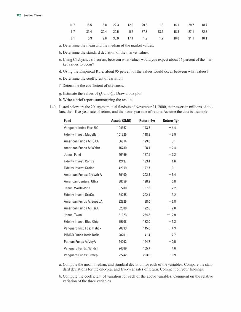
11.7 18.5 6.8 22.3 12.9 29.8 1.3 14.1 29.7 18.7
6.7 31.4 30.4 20.6 5.2 37.8 13.4 18.3 27.1 32.7
6.1 0.9 9.6 35.0 17.1 1.9 1.2 16.6 31.1 16.1
a. Determine the mean and the median of the market values.
b. Determine the standard deviation of the market values.
c. Using Chebyshev’s theorem, between what values would you expect about 56 percent of the mar-ket values to occur?
d. Using the Empirical Rule, about 95 percent of the values would occur between what values?
e. Determine the coefficient of variation.
f. Determine the coefficient of skewness.
g. Estimate the values of Q1 and Q3. Draw a box plot.
h. Write a brief report summarizing the results.
140. Listed below are the 20 largest mutual funds as of November 21, 2000, their assets in millions of dol-lars, their five-year rate of return, and their one-year rate of return. Assume the data is a sample.
Fund Assets ($Mil) Return-5yr Return-1yr
Vanguard Index Fds: 500 104357 143.5 �4.4
Fidelity Invest: Magellan 101625 118.8 �3.9
American Funds A: ICAA 56614 129.8 3.1
American Funds A: WshA 46780 108.1 �2.4
Janus: Fund 46499 177.5 �2.2
Fidelity Invest: Contra 42437 133.4 1.6
Fidelity Invest: Grolnc 42059 127.7 0.1
American Funds: Growth A 39400 202.8 �6.4
American Century: Ultra 38559 128.2 �5.8
Janus: WorldWide 37780 187.3 2.2
Fidelity Invest: GroCo 34255 202.1 13.2
American Funds A: EupacA 32826 98.0 �2.8
American Funds A: PerA 32308 122.8 �2.0
Janus: Twen 31023 264.3 �12.9
Fidelity Invest: Blue Chip 29708 132.0 �1.2
Vanguard Instl Fds: Instidx 28893 145.0 �4.3
PIMCO Funds Instl: TotRt 28201 41.4 7.7
Putman Funds A: VoyA 24262 144.7 �0.5
Vanguard Funds: Wndsll 24069 105.7 4.6
Vanguard Funds: Prmcp 22742 203.0 10.9
a. Compute the mean, median, and standard deviation for each of the variables. Compare the stan-dard deviations for the one-year and five-year rates of return. Comment on your findings.
b. Compute the coefficient of variation for each of the above variables. Comment on the relativevariation of the three variables.
342 Section Three

c. Compute the coefficient of skewness for each of the above variables. Comment on the skewnessof the three variables.
d. Compute the first and third quartiles for the one-year and five-year rates of return.
e. Draw a box plot for the one-year and five-year rates of return. Comment on the results. Are thereany outliers?
141. The Apollo space program lasted from 1967 until 1972 and included 13 missions. The missionslasted from as little as 7 hours to as long as 301 hours. The duration of each flight is listed below.
9 195 241 301 216 260 7 244 192 147
10 295 142
a. Find the mean, median, and standard deviation of the duration for the Apollo flights.
b. Compute the coefficient of variation and the coefficient of skewness. Comment on your findings.
c. Find the 45th and 82nd percentiles.
d. Draw a box plot and comment on your findings.
142. Listed below is the average daily circulation for the 50 U.S. newspapers with the largest circulation.
a. Find the mean, median, Q1, and Q3.
b. Find the 15th and the 90th percentiles.
c. Find the coefficient of skewness and interpret the result.
d. Develop a box plot and interpret the result.
Newspaper Circulation
Wall Street Journal (New York, N.Y.) 1,740,450USA Today (Arlington, Va.) 1,653,428Times (Los Angeles) 1,067,540Times (New York, N.Y.) 1,066,658Post (Washington, D.C.) 759,122Daily News (New York, N.Y.) 723,143Tribune (Chicago) 673,508Newsday (Long Island, N.Y.) 572,444Chronicle (Houston) 550,763Sun-Times (Chicago) 485,666Morning News (Dallas) 479,863Chronicle (San Francisco) 475,324Globe (Boston) 470,825Post (New York, N.Y.) 437,467Arizona Republic (Phoenix) 435,330Inquirer (Philadelphia) 428,895Star-Ledger (Newark, N.J.) 407,026Plain Dealer (Cleveland) 382,933Free Press (Detroit) 378,256Union-Tribune (San Diego) 378,112Register (Orange County, Calif.) 356,953Herald (Miami) 349,114Oregonian (Portland) 346,593Times (St. Petersburg, Fla.) 344,784Post (Denver) 341,554
Newspaper Circulation
Star Tribune (Minneapolis) 334,751Rocky Mountain News (Denver) 331,978Post-Dispatch (St. Louis) 329,582Sun (Baltimore) 314,033Constitution (Atlanta) 303,698Mercury News (San Jose, Calif.) 290,885Journal Sentinel (Milwaukee) 285,776Bee (Sacramento, Calif.) 283,589Star (Kansas City, Mo.) 281,596Herald (Boston) 271,425Times-Picayune (New Orleans) 259,317Sun-Sentinel (Fort Lauderdale, Fla.) 258,726Sentinel (Orlando, Fla.) 258,726Investor’s Business Daily (Los Angeles) 251,172Dispatch (Columbus, Ohio) 246,528News (Detroit) 245,351Observer (Charlotte, N.C.) 243,818Post-Gazette (Pittsburgh, Pa.) 243,453News (Buffalo, N.Y.) 237,229Tribune (Tampa, Fla.) 235,786Star-Telegram (Fort Worth, Tex.) 232,112Star (Indianapolis) 230,223Courier-Journal (Louisville, Ky.) 228,144Times (Seattle) 227,715World-Herald (Omaha, Neb.) 219,891
Introduction to Descriptive Statistics and Discrete Probability Distributions 343
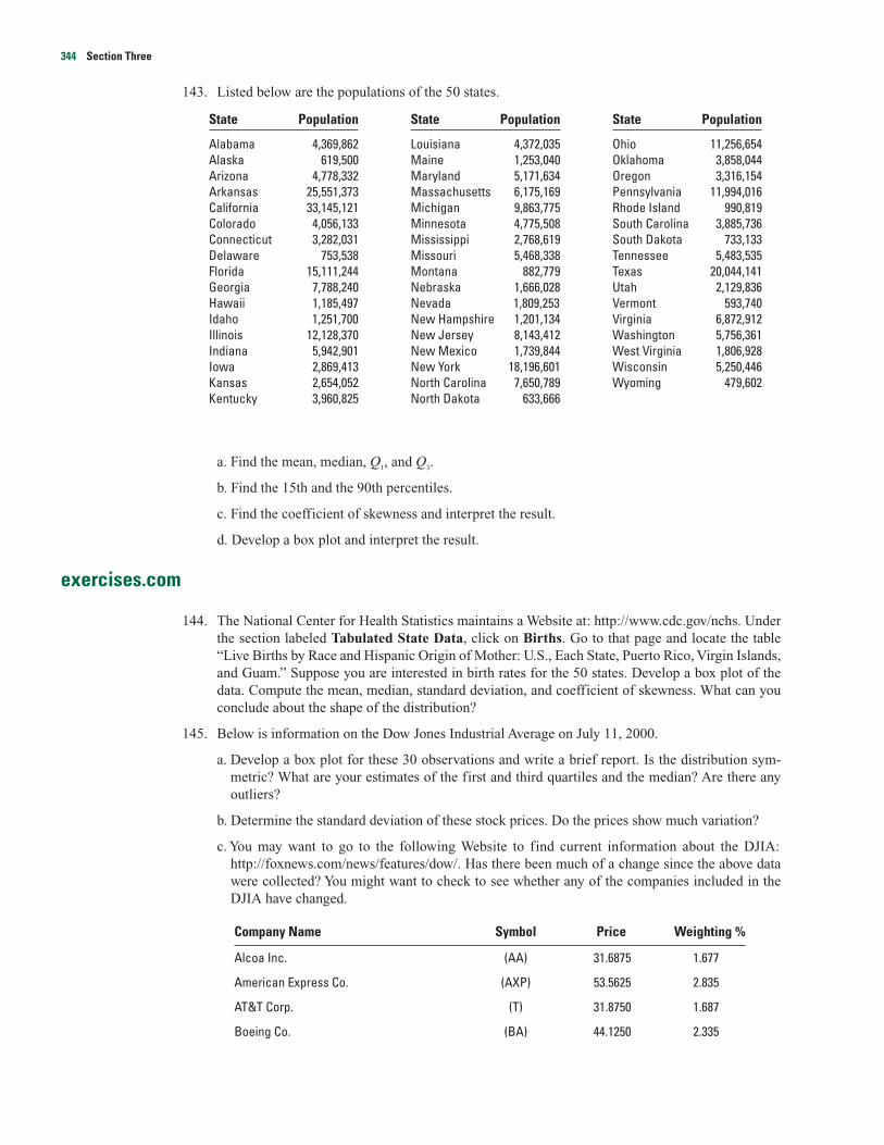
143. Listed below are the populations of the 50 states.
a. Find the mean, median, Q1, and Q3.
b. Find the 15th and the 90th percentiles.
c. Find the coefficient of skewness and interpret the result.
d. Develop a box plot and interpret the result.
exercises.com
144. The National Center for Health Statistics maintains a Website at: http://www.cdc.gov/nchs. Underthe section labeled Tabulated State Data, click on Births. Go to that page and locate the table“Live Births by Race and Hispanic Origin of Mother: U.S., Each State, Puerto Rico, Virgin Islands,and Guam.” Suppose you are interested in birth rates for the 50 states. Develop a box plot of thedata. Compute the mean, median, standard deviation, and coefficient of skewness. What can youconclude about the shape of the distribution?
145. Below is information on the Dow Jones Industrial Average on July 11, 2000.
a. Develop a box plot for these 30 observations and write a brief report. Is the distribution sym-metric? What are your estimates of the first and third quartiles and the median? Are there anyoutliers?
b. Determine the standard deviation of these stock prices. Do the prices show much variation?
c. You may want to go to the following Website to find current information about the DJIA:http://foxnews.com/news/features/dow/. Has there been much of a change since the above datawere collected? You might want to check to see whether any of the companies included in theDJIA have changed.
Company Name Symbol Price Weighting %
Alcoa Inc. (AA) 31.6875 1.677
American Express Co. (AXP) 53.5625 2.835
AT&T Corp. (T) 31.8750 1.687
Boeing Co. (BA) 44.1250 2.335
State Population
Alabama 4,369,862Alaska 619,500Arizona 4,778,332Arkansas 25,551,373California 33,145,121Colorado 4,056,133Connecticut 3,282,031Delaware 753,538Florida 15,111,244Georgia 7,788,240Hawaii 1,185,497Idaho 1,251,700Illinois 12,128,370Indiana 5,942,901Iowa 2,869,413Kansas 2,654,052Kentucky 3,960,825
State Population
Louisiana 4,372,035Maine 1,253,040Maryland 5,171,634Massachusetts 6,175,169Michigan 9,863,775Minnesota 4,775,508Mississippi 2,768,619Missouri 5,468,338Montana 882,779Nebraska 1,666,028Nevada 1,809,253New Hampshire 1,201,134New Jersey 8,143,412New Mexico 1,739,844New York 18,196,601North Carolina 7,650,789North Dakota 633,666
State Population
Ohio 11,256,654Oklahoma 3,858,044Oregon 3,316,154Pennsylvania 11,994,016Rhode Island 990,819South Carolina 3,885,736South Dakota 733,133Tennessee 5,483,535Texas 20,044,141Utah 2,129,836Vermont 593,740Virginia 6,872,912Washington 5,756,361West Virginia 1,806,928Wisconsin 5,250,446Wyoming 479,602
344 Section Three
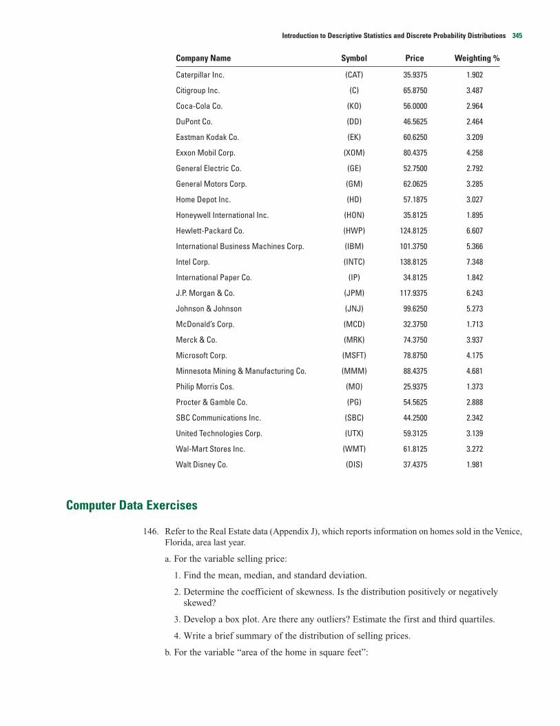
Company Name Symbol Price Weighting %
Caterpillar Inc. (CAT) 35.9375 1.902
Citigroup Inc. (C) 65.8750 3.487
Coca-Cola Co. (KO) 56.0000 2.964
DuPont Co. (DD) 46.5625 2.464
Eastman Kodak Co. (EK) 60.6250 3.209
Exxon Mobil Corp. (XOM) 80.4375 4.258
General Electric Co. (GE) 52.7500 2.792
General Motors Corp. (GM) 62.0625 3.285
Home Depot Inc. (HD) 57.1875 3.027
Honeywell International Inc. (HON) 35.8125 1.895
Hewlett-Packard Co. (HWP) 124.8125 6.607
International Business Machines Corp. (IBM) 101.3750 5.366
Intel Corp. (INTC) 138.8125 7.348
International Paper Co. (IP) 34.8125 1.842
J.P. Morgan & Co. (JPM) 117.9375 6.243
Johnson & Johnson (JNJ) 99.6250 5.273
McDonald’s Corp. (MCD) 32.3750 1.713
Merck & Co. (MRK) 74.3750 3.937
Microsoft Corp. (MSFT) 78.8750 4.175
Minnesota Mining & Manufacturing Co. (MMM) 88.4375 4.681
Philip Morris Cos. (MO) 25.9375 1.373
Procter & Gamble Co. (PG) 54.5625 2.888
SBC Communications Inc. (SBC) 44.2500 2.342
United Technologies Corp. (UTX) 59.3125 3.139
Wal-Mart Stores Inc. (WMT) 61.8125 3.272
Walt Disney Co. (DIS) 37.4375 1.981
Computer Data Exercises
146. Refer to the Real Estate data (Appendix J), which reports information on homes sold in the Venice,Florida, area last year.
a. For the variable selling price:
1. Find the mean, median, and standard deviation.
2. Determine the coefficient of skewness. Is the distribution positively or negativelyskewed?
3. Develop a box plot. Are there any outliers? Estimate the first and third quartiles.
4. Write a brief summary of the distribution of selling prices.
b. For the variable “area of the home in square feet”:
Introduction to Descriptive Statistics and Discrete Probability Distributions 345

1. Find the mean, median, and the standard deviation.
2. Determine the coefficient of skewness. Is the distribution positively or negativelyskewed?
3. Develop a box plot. Are there any outliers? Estimate the first and third quartiles.
4. Write a brief summary of the distribution of the area of homes.
147. Refer to the Baseball 2000 data (Appendix K), which reports information on the 30 Major LeagueBaseball teams for the 2000 baseball season.
a. For the variable team salary:
1. Find the mean, median, and standard deviation.
2. Determine the coefficient of skewness. Is the distribution positively or negativelyskewed?
3. Develop a box plot. Are there any outliers? Estimate the first and third quartiles.
4. Write a brief summary of the distribution of team salaries.
b. For the variable that refers to the year in which the stadium was built (Hint: Subtractthe current year from the year in which the stadium was built to find the stadium ageand work with that variable):
1. Find the mean, median, and standard deviation.
2. Determine the coefficient of skewness. Is the distribution positively or negativelyskewed?
3. Develop a box plot. Are there any outliers? Estimate the first and third quartiles.
4. Write a brief summary of the distribution of the age of the stadium.
148. Refer to the OECD data (Appendix L), which reports information on the census, economic, andbusiness data for 29 countries.
a. For the variable employment:
1. Find the mean, median, and standard deviation.
2. Determine the coefficient of skewness. Is the distribution positively or negativelyskewed?
3. Develop a box plot. Are there any outliers? Estimate the first and third quartiles.
4. Write a brief summary of the distribution of employment.
b. For the variable percent of the population over the age of 65:
1. Find the mean, median, and standard deviation.
2. Determine the coefficient of skewness. Is the distribution positively or negativelyskewed?
3. Develop a box plot. Are there any outliers? Estimate the first and third quartiles.
4. Write a brief summary of the distribution of percent of population over 65.
149. Refer to the Schools data (Appendix M), which reports information on 94 school districts in North-west Ohio.
a. For the variable teacher salary:
1. Find the mean, median, and standard deviation.
2. Determine the coefficient of skewness. Is the distribution positively or negativelyskewed?
3. Develop a box plot. Are there any outliers? Estimate the first and third quartiles.
346 Section Three

4. Write a brief summary of the distribution.
b. For the variable number of students in the school district:
1. Find the mean, median, and standard deviation.
2. Determine the coefficient of skewness. Is the distribution positively or negativelyskewed?
3. Develop a box plot. Are there any outliers? Estimate the first and third quartiles.
4. Write a brief summary of the distribution.
Computer Commands
2. The MINITAB commands for the descriptive summary about software company earnings are:
a. Enter the earnings reported in the Example column C1 of the spreadsheet. Name the variableEarnings.
b. Select Stat, Basic Statistics, and then Display Descriptive Statistics. In the dialog box selectEarnings as the variable and then click on Graphs in the lower right corner. Within this dialogbox select Graphic summary and click OK. Click OK in the next dialog box.
Introduction to Descriptive Statistics and Discrete Probability Distributions 347
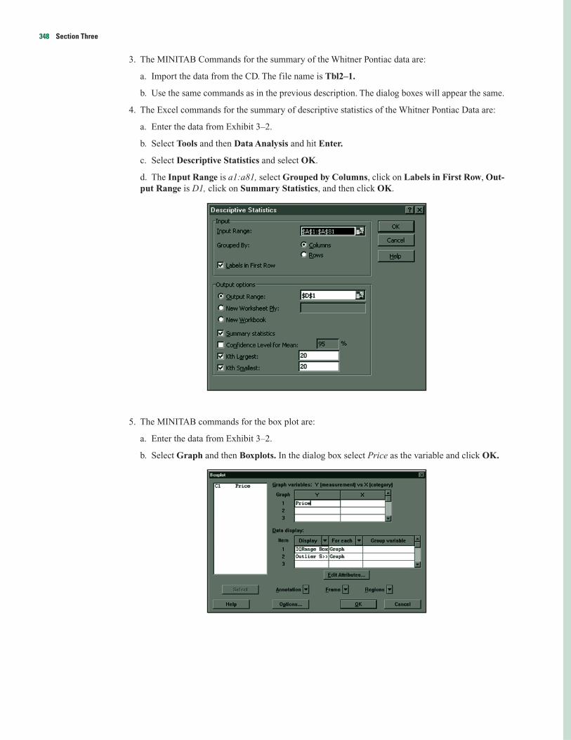
3. The MINITAB Commands for the summary of the Whitner Pontiac data are:
a. Import the data from the CD. The file name is Tbl2–1.
b. Use the same commands as in the previous description. The dialog boxes will appear the same.
4. The Excel commands for the summary of descriptive statistics of the Whitner Pontiac Data are:
a. Enter the data from Exhibit 3–2.
b. Select Tools and then Data Analysis and hit Enter.
c. Select Descriptive Statistics and select OK.
d. The Input Range is a1:a81, select Grouped by Columns, click on Labels in First Row, Out-put Range is D1, click on Summary Statistics, and then click OK.
5. The MINITAB commands for the box plot are:
a. Enter the data from Exhibit 3–2.
b. Select Graph and then Boxplots. In the dialog box select Price as the variable and click OK.
348 Section Three
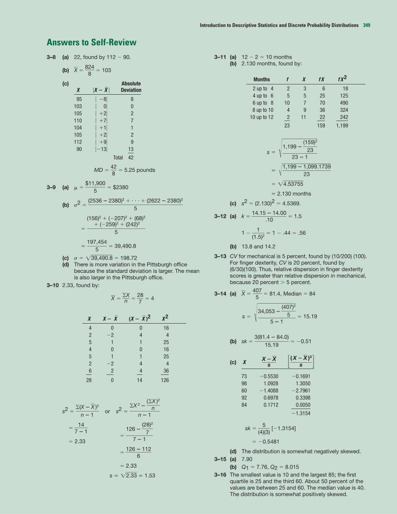
Answers to Self-Review3–8 (a) 22, found by 112 � 90.
(b) � � 103
(c) AbsoluteX �X � � Deviation
95 � �8� 8103 � 0� 0105 � �2� 2110 � �7� 7104 � �1� 1105 � �2� 2112 � �9� 990 ��13� 13
Total 42
MD � � 5.25 pounds
3–9 (a) � � � $2380
(b) �2 �
�
� � 39,490.8
(c) � � � 198.72(d) There is more variation in the Pittsburgh office
because the standard deviation is larger. The meanis also larger in the Pittsburgh office.
3–10 2.33, found by:
� � � 4
X X � (X � )2 X 2
4 0 0 162 �2 4 45 1 1 254 0 0 165 1 1 252 �2 4 46 2 4 36
28 0 14 126
s2 � or s2 �
�
�� 2.33
�
� 2.33
s � � 1.53
3–11 (a) 12 � 2 � 10 months(b) 2.130 months, found by:
Months f X f X f X 2
2 up to 4 2 3 6 184 up to 6 5 5 25 1256 up to 8 10 7 70 4908 up to 10 4 9 36 324
10 up to 12 2 11 22 242
23 159 1,199
s �
�
�
� 2.130 months
(c) s2 � (2.130)2 � 4.5369.
3–12 (a) k � � 1.5
1 � � 1 � .44 � .56
(b) 13.8 and 14.2
3–13 CV for mechanical is 5 percent, found by (10/200) (100).For finger dexterity, CV is 20 percent, found by(6/30)(100). Thus, relative dispersion in finger dexterityscores is greater than relative dispersion in mechanical,because 20 percent 5 percent.
3–14 (a) � � 81.4, Median � 84
s � � 15.19
(b) sk � � �0.51
(c) X
73 �0.5530 �0.169198 1.0928 1.305060 �1.4088 �2.796192 0.6978 0.339884 0.1712 0.0050
�1.3154
sk � [�1.3154]
� �0.5481
(d) The distribution is somewhat negatively skewed.3–15 (a) 7.90
(b) Q1 � 7.76, Q2 � 8.0153–16 The smallest value is 10 and the largest 85; the first
quartile is 25 and the third 60. About 50 percent of thevalues are between 25 and 60. The median value is 40.The distribution is somewhat positively skewed.
5(4)(3)
�( X � X )3
s X � Xs
3(81.4 � 84.0)15.19
�34,053 �(407)2
55 � 1
4075
X
1(1.5)2
14.15 � 14.00.10
�4.53755
�1,199 � 1,099.173923
�1,199 �(159)2
2323 � 1
�2.33
126 � 1126
126 �(28)2
77 � 1
147 � 1
�X 2 �(�X )2
nn � 1
�(X � X )2
n � 1
XX
287
�XnX
�39,490.8
197,4545
(156)2 � (�207)2 � (68)2� (�259)2 � (242)2
5
(2536 � 2380)2 � · · · � (2622 � 2380)2
5
$11,9005
428
X
8248
X
Introduction to Descriptive Statistics and Discrete Probability Distributions 349
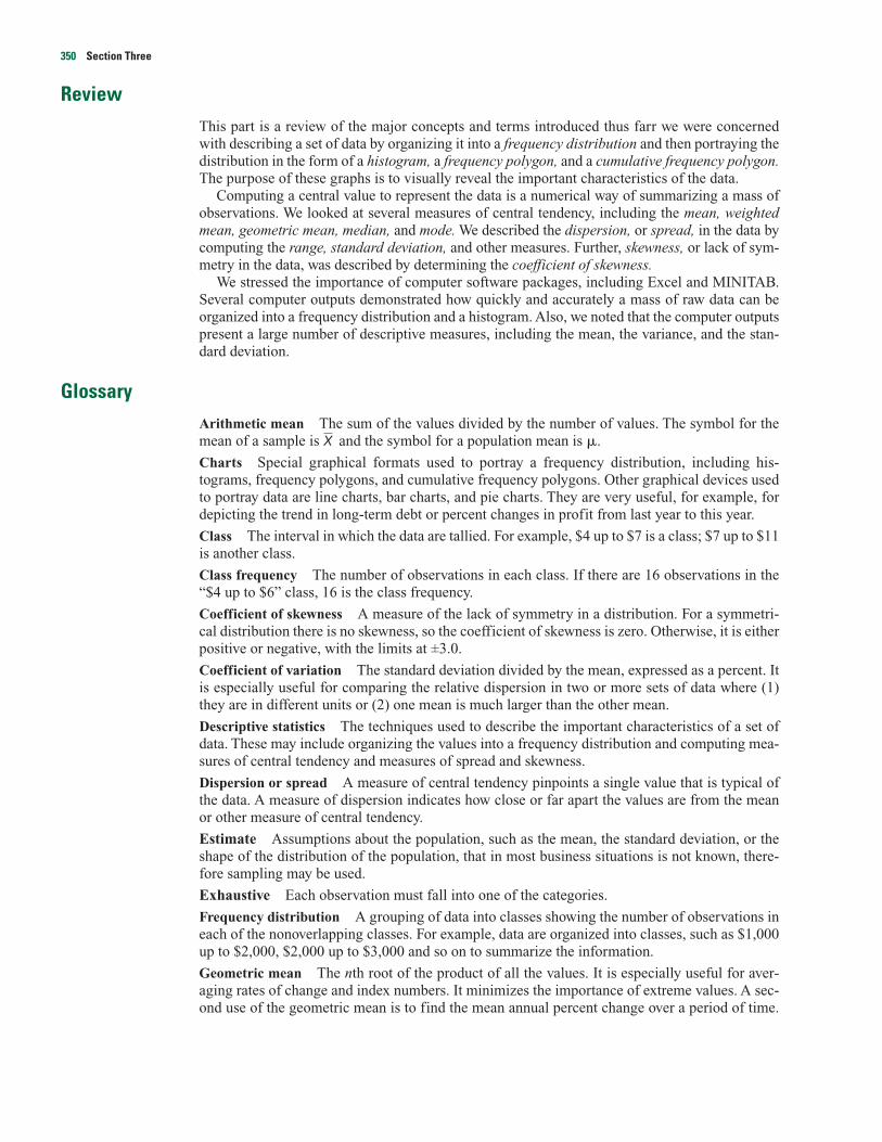
ReviewThis part is a review of the major concepts and terms introduced thus farr we were concernedwith describing a set of data by organizing it into a frequency distribution and then portraying thedistribution in the form of a histogram, a frequency polygon, and a cumulative frequency polygon.The purpose of these graphs is to visually reveal the important characteristics of the data.
Computing a central value to represent the data is a numerical way of summarizing a mass ofobservations. We looked at several measures of central tendency, including the mean, weightedmean, geometric mean, median, and mode. We described the dispersion, or spread, in the data bycomputing the range, standard deviation, and other measures. Further, skewness, or lack of sym-metry in the data, was described by determining the coefficient of skewness.
We stressed the importance of computer software packages, including Excel and MINITAB.Several computer outputs demonstrated how quickly and accurately a mass of raw data can beorganized into a frequency distribution and a histogram. Also, we noted that the computer outputspresent a large number of descriptive measures, including the mean, the variance, and the stan-dard deviation.
GlossaryArithmetic mean The sum of the values divided by the number of values. The symbol for themean of a sample is and the symbol for a population mean is �.
Charts Special graphical formats used to portray a frequency distribution, including his-tograms, frequency polygons, and cumulative frequency polygons. Other graphical devices usedto portray data are line charts, bar charts, and pie charts. They are very useful, for example, fordepicting the trend in long-term debt or percent changes in profit from last year to this year.
Class The interval in which the data are tallied. For example, $4 up to $7 is a class; $7 up to $11is another class.
Class frequency The number of observations in each class. If there are 16 observations in the“$4 up to $6” class, 16 is the class frequency.
Coefficient of skewness A measure of the lack of symmetry in a distribution. For a symmetri-cal distribution there is no skewness, so the coefficient of skewness is zero. Otherwise, it is eitherpositive or negative, with the limits at ±3.0.
Coefficient of variation The standard deviation divided by the mean, expressed as a percent. Itis especially useful for comparing the relative dispersion in two or more sets of data where (1)they are in different units or (2) one mean is much larger than the other mean.
Descriptive statistics The techniques used to describe the important characteristics of a set ofdata. These may include organizing the values into a frequency distribution and computing mea-sures of central tendency and measures of spread and skewness.
Dispersion or spread A measure of central tendency pinpoints a single value that is typical ofthe data. A measure of dispersion indicates how close or far apart the values are from the meanor other measure of central tendency.
Estimate Assumptions about the population, such as the mean, the standard deviation, or theshape of the distribution of the population, that in most business situations is not known, there-fore sampling may be used.
Exhaustive Each observation must fall into one of the categories.
Frequency distribution A grouping of data into classes showing the number of observations ineach of the nonoverlapping classes. For example, data are organized into classes, such as $1,000up to $2,000, $2,000 up to $3,000 and so on to summarize the information.
Geometric mean The nth root of the product of all the values. It is especially useful for aver-aging rates of change and index numbers. It minimizes the importance of extreme values. A sec-ond use of the geometric mean is to find the mean annual percent change over a period of time.
X
350 Section Three

For example, if gross sales were $245 million in 1985 and $692 million in 2000, what is the aver-age annual percent increase?
Groups May also be called classes
Hypothesis A statement about the value of a population developed for the purpose of testing.
Interquartile range The distance between the third quartile and the first quartile.
Inferential statistics, also called statistical inference or inductive statistics This facet of statis-tics deals with estimating a population parameter based on a sample statistic. For example, if 2out of the 10 hand calculators sampled are defective, we might infer that 20 percent of the pro-duction is defective.
Interval measurement If one observation is greater than another by a certain amount, and thezero point is arbitrary, the measurement is on an interval scale. For example, the differencebetween temperatures of 70 degrees and 80 degrees is 10 degrees. Likewise, a temperature of 90degrees is 10 degrees more than a temperature of 80 degrees, and so on.
Mean deviation The mean of the deviations from the mean, disregarding signs. It is abbreviatedas MD.
Measure of central tendency A number that describes the central tendency of the data. Thereare several such measures, including the arithmetic mean, weighted mean, median, mode, andgeometric mean.
Median The value of the middle observation after all the observations have been arranged fromlow to high. For example, if observations 6, 9, 4 are rearranged to read 4, 6, 9, the middle valueis 6, the median.
Mode The value that appears most frequently in a set of data. For grouped data, it is the mid-point of the class containing the largest number of values.
Mutually exclusive A property of a set of categories such that an individual, object, or mea-surement is included in only one category.
Midpoint The value that divides the class into two equal parts. For the classes $10 up to $20 and$20 up to $30, the midpoints are $15 and $25, respectively.
Nominal measurement The “lowest” level of measurement. If data are classified into categoriesand the order of those categories is not important, it is the nominal level of measurement. Exam-ples are gender (male, female) and political affiliation (Republican, Democrat, Independent, allothers). If it makes no difference whether male or female is listed first, the data are nominal level.
Ordinal measurement Data that can be logically ranked are referred to as ordinal measures.For example, consumer response to the sound of a new speaker might be excellent, very good,fair, or poor.
Parameter A characteristic of a population.
Population The collection, or set, of all individuals, objects, or measurements whose propertiesare being studied.
Quartiles Values that divide a set of data into four equal parts.
Quantitative variable A variable being studied that can be reported numerically.
Qualitative variable A variable that has the characteristic of being nonnumeric.
Random variable A quantity resulting from an experiment that, by chance, can assume differ-ent values.
Range Difference between the highest and lowest values.
Ratio measurement If the distances between numbers are of a known constant size and there isa true zero point, and the ratio of two values is meaningful, the measurement is ratio scale. Forexample, the distance between $200 and $300 is $100, and in the case of money there is a truezero point. If you have zero dollars, there is an absence of money (you have none). Also the ratiobetween $200 and $300 is meaningful.
Sample A portion, or subset, of the population being studied.
Standard deviation Square root of the variance.
Introduction to Descriptive Statistics and Discrete Probability Distributions 351

Statistics The science of collecting, organizing, analyzing, and interpreting numerical data forthe purpose of making more effective decisions.
Unbiased Sample selected so that each item or person in the population has the same chanceof being included. A sample based on the judgment of the person selecting the sample may bebiased, meaning that the sample results may not be representative of the population.
Ungrouped data Also referred to as raw data.
Variance Mean of the squared deviations from the mean.
Weighted mean Each value is weighted according to its relative importance. For example, if 5shirts cost $10 each and 20 shirts cost $8 each, the weighted mean price is $8.40: [(5 � $10) �(20 � $8)]/25 � $210/25 � $8.40.
∑ indicates the operation of adding all the values. It is pronounced “sigma.”
µ stands for the population mean
Standard deviation (σ)
(π) is the probability of success on each trial in a binomial probability distribution.
E maximum allowable error.
Chi-square designated x2, is used as the test statistic. Chi-square is based on squared devia-tions between an observed frequency and an expected frequency and, therefore, it is always pos-itive.
Null hypothesis designated H0, and read H sub zero. The letter H stands for hypothesis, and thesubscript zero implies “no difference”.
Alternate hypothesis written H1. A statement that is accepted if the sample data provides evi-dence that the null hypothesis is false.
Exercises
1. A small number of employees were selected from all the employees at NED Electronics and theirhourly rates recorded. The rates were: $9.50, $9.00, $11.70, $14.80, and $13.00.
a. Are the hourly rates a sample or a population?
b. What is the level of measurement?
c. What is the arithmetic mean hourly rate?
d. What is the median hourly rate? Interpret.
e. What is the variance?
f. What is the coefficient of skewness? Interpret.
2. The weekly overtime hours worked by all the employees at the Publix Market are: 1, 4, 6, 12, 5,and 2.
a. Is this a sample or a population?
b. What is the mean number of overtime hours worked?
c. What is the median? Interpret.
d. What is the mode?
e. What is the mean deviation?
f. What is the standard deviation?
g. What is the coefficient of variation?
352 Section Three

3. The Tourist Bureau of St. Thomas surveyed a sample of tourists as they left to return to the UnitedStates. One of the questions was: How many rolls of film did you expose when visiting our island?The responses were:
8 6 3 11 14 8 9 16 9 10
5 11 7 8 8 10 9 12 13 9
a. Using five classes, organize the sample data into a frequency distribution.
b. Portray the distribution in the form of a frequency polygon.
c. What is the mean number of rolls exposed? Use the actual raw data.
d. What is the median? Use the actual raw data.
e. What is the mode? Use the actual raw data.
f. What is the range? Use the actual raw data.
g. What is the sample variance? Use the actual raw data.
h. What is the sample standard deviation? Use the actual raw data.
i. Assuming that the distribution is symmetrical and bell-shaped, about 95 percent of the touristsexposed between _______ and _______ rolls.
4. The annual amounts spent on research and development for a sample of electronic component man-ufacturers are (in $ millions):
8 34 15 24 15 28 12 20 22 23
14 26 18 23 10 21 16 17 22 31
13 25 20 28 6 20 19 27 16 22
a. What is the level of measurement?
b. Using six classes, organize the expenditures into a frequency distribution.
c. Portray the distribution in the form of a histogram.
d. What is the mean amount spent on research and development?
5. The rates of growth of Bardeen Chemicals for the past five years are 5.2 percent, 8.7 percent, 3.9percent, 6.8 percent, and 19.5 percent.
a. What is the arithmetic mean annual growth rate?
b. What is the geometric mean annual growth rate?
c. Should the arithmetic mean or geometric mean be used to represent the average annual growthrate? Why?
6. The Currin Manufacturing Co. noted in its 2000 second-quarter report that as of June 30, 2000,notes payable amounted to $284.0 million. For the same date in 1990, they were $113.0 million.What is the geometric mean yearly percent increase (June to June) from June 1990 to June 2000?
7. BFI in its annual report revealed that working capital was (in billions) $4.4, $3.4, $3.0, $4.8, $7.8,and $8.3 consecutively for the years 1995–2000. Present these figures in either a simple line chartor a simple bar chart.
8. Refer to the following diagram.
a. What is the graph called?
0 40 80 120 160 200
* *
Introduction to Descriptive Statistics and Discrete Probability Distributions 353
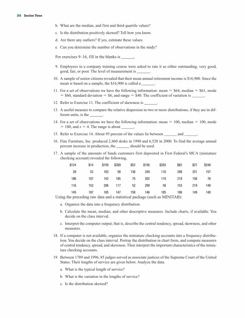
b. What are the median, and first and third quartile values?
c. Is the distribution positively skewed? Tell how you know.
d. Are there any outliers? If yes, estimate these values.
e. Can you determine the number of observations in the study?
For exercises 9–16, fill in the blanks is _______.
9. Employees in a company training course were asked to rate it as either outstanding, very good,good, fair, or poor. The level of measurement is _______.
10. A sample of senior citizens revealed that their mean annual retirement income is $16,900. Since themean is based on a sample, the $16,900 is called a _______.
11. For a set of observations we have the following information: mean � $64, median � $61, mode� $60, standard deviation � $6, and range � $40. The coefficient of variation is _______.
12. Refer to Exercise 11. The coefficient of skewness is _______.
13. A useful measure to compare the relative dispersion in two or more distributions, if they are in dif-ferent units, is the _______.
14. For a set of observations we have the following information: mean � 100, median � 100, mode� 100, and s � 4. The range is about _______.
15. Refer to Exercise 14. About 95 percent of the values lie between _______ and _______.
16. Fine Furniture, Inc. produced 2,460 desks in 1990 and 6,520 in 2000. To find the average annualpercent increase in production, the _______ should be used.
17. A sample of the amounts of funds customers first deposited in First Federal’s MCA (miniaturechecking account) revealed the following.
$124 $14 $150 $289 $52 $156 $203 $82 $27 $248
39 52 103 58 136 249 110 298 251 157
186 107 142 185 75 202 119 219 156 78
116 152 206 117 52 299 58 153 219 148
145 187 165 147 158 146 185 186 149 140Using the preceding raw data and a statistical package (such as MINITAB):
a. Organize the data into a frequency distribution.
b. Calculate the mean, median, and other descriptive measures. Include charts, if available. Youdecide on the class interval.
c. Interpret the computer output; that is, describe the central tendency, spread, skewness, and othermeasures.
18. If a computer is not available, organize the miniature checking accounts into a frequency distribu-tion. You decide on the class interval. Portray the distribution in chart form, and compute measuresof central tendency, spread, and skewness. Then interpret the important characteristics of the minia-ture checking accounts.
19. Between 1789 and 1996, 85 judges served as associate justices of the Supreme Court of the UnitedStates. Their lengths of service are given below. Analyze the data.
a. What is the typical length of service?
b. What is the variation in the lengths of service?
c. Is the distribution skewed?
354 Section Three
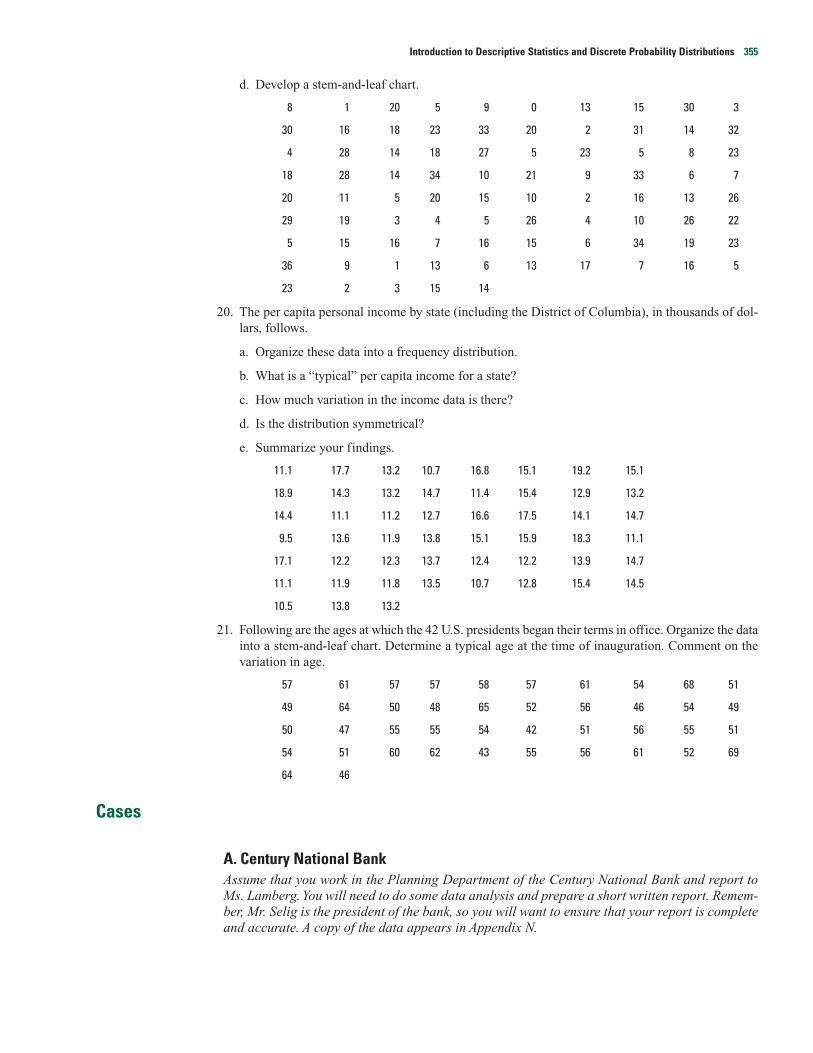
d. Develop a stem-and-leaf chart.
8 1 20 5 9 0 13 15 30 3
30 16 18 23 33 20 2 31 14 32
4 28 14 18 27 5 23 5 8 23
18 28 14 34 10 21 9 33 6 7
20 11 5 20 15 10 2 16 13 26
29 19 3 4 5 26 4 10 26 22
5 15 16 7 16 15 6 34 19 23
36 9 1 13 6 13 17 7 16 5
23 2 3 15 14
20. The per capita personal income by state (including the District of Columbia), in thousands of dol-lars, follows.
a. Organize these data into a frequency distribution.
b. What is a “typical” per capita income for a state?
c. How much variation in the income data is there?
d. Is the distribution symmetrical?
e. Summarize your findings.
11.1 17.7 13.2 10.7 16.8 15.1 19.2 15.1
18.9 14.3 13.2 14.7 11.4 15.4 12.9 13.2
14.4 11.1 11.2 12.7 16.6 17.5 14.1 14.7
9.5 13.6 11.9 13.8 15.1 15.9 18.3 11.1
17.1 12.2 12.3 13.7 12.4 12.2 13.9 14.7
11.1 11.9 11.8 13.5 10.7 12.8 15.4 14.5
10.5 13.8 13.2
21. Following are the ages at which the 42 U.S. presidents began their terms in office. Organize the datainto a stem-and-leaf chart. Determine a typical age at the time of inauguration. Comment on thevariation in age.
57 61 57 57 58 57 61 54 68 51
49 64 50 48 65 52 56 46 54 49
50 47 55 55 54 42 51 56 55 51
54 51 60 62 43 55 56 61 52 69
64 46
Cases
A. Century National BankAssume that you work in the Planning Department of the Century National Bank and report toMs. Lamberg. You will need to do some data analysis and prepare a short written report. Remem-ber, Mr. Selig is the president of the bank, so you will want to ensure that your report is completeand accurate. A copy of the data appears in Appendix N.
Introduction to Descriptive Statistics and Discrete Probability Distributions 355
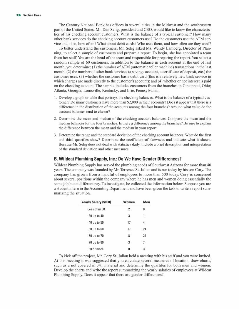
The Century National Bank has offices in several cities in the Midwest and the southeasternpart of the United States. Mr. Dan Selig, president and CEO, would like to know the characteris-tics of his checking account customers. What is the balance of a typical customer? How manyother bank services do the checking account customers use? Do the customers use the ATM ser-vice and, if so, how often? What about debit cards? Who uses them, and how often are they used?
To better understand the customers, Mr. Selig asked Ms. Wendy Lamberg, Director of Plan-ning, to select a sample of customers and prepare a report. To begin, she has appointed a teamfrom her staff. You are the head of the team and responsible for preparing the report. You select arandom sample of 60 customers. In addition to the balance in each account at the end of lastmonth, you determine: (1) the number of ATM (automatic teller machine) transactions in the lastmonth; (2) the number of other bank services (a savings account, a certificate of deposit, etc.) thecustomer uses; (3) whether the customer has a debit card (this is a relatively new bank service inwhich charges are made directly to the customer’s account); and (4) whether or not interest is paidon the checking account. The sample includes customers from the branches in Cincinnati, Ohio;Atlanta, Georgia; Louisville, Kentucky; and Erie, Pennsylvania.
1. Develop a graph or table that portrays the checking balances. What is the balance of a typical cus-tomer? Do many customers have more than $2,000 in their accounts? Does it appear that there is adifference in the distribution of the accounts among the four branches? Around what value do theaccount balances tend to cluster?
2. Determine the mean and median of the checking account balances. Compare the mean and themedian balances for the four branches. Is there a difference among the branches? Be sure to explainthe difference between the mean and the median in your report.
3. Determine the range and the standard deviation of the checking account balances. What do the firstand third quartiles show? Determine the coefficient of skewness and indicate what it shows.Because Mr. Selig does not deal with statistics daily, include a brief description and interpretationof the standard deviation and other measures.
B. Wildcat Plumbing Supply, Inc.: Do We Have Gender Differences?Wildcat Plumbing Supply has served the plumbing needs of Southwest Arizona for more than 40years. The company was founded by Mr. Terrence St. Julian and is run today by his son Cory. Thecompany has grown from a handful of employees to more than 500 today. Cory is concernedabout several positions within the company where he has men and women doing essentially thesame job but at different pay. To investigate, he collected the information below. Suppose you area student intern in the Accounting Department and have been given the task to write a report sum-marizing the situation.
Yearly Salary ($000) Women Men
Less than 30 2 0
30 up to 40 3 1
40 up to 50 17 4
50 up to 60 17 24
60 up to 70 8 21
70 up to 80 3 7
80 or more 0 3
To kick off the project, Mr. Cory St. Julian held a meeting with his staff and you were invited.At this meeting it was suggested that you calculate several measures of location, draw charts,such as a not covered in 341 material and determine the quartiles for both men and women.Develop the charts and write the report summarizing the yearly salaries of employees at WildcatPlumbing Supply. Does it appear that there are gender differences?
356 Section Three
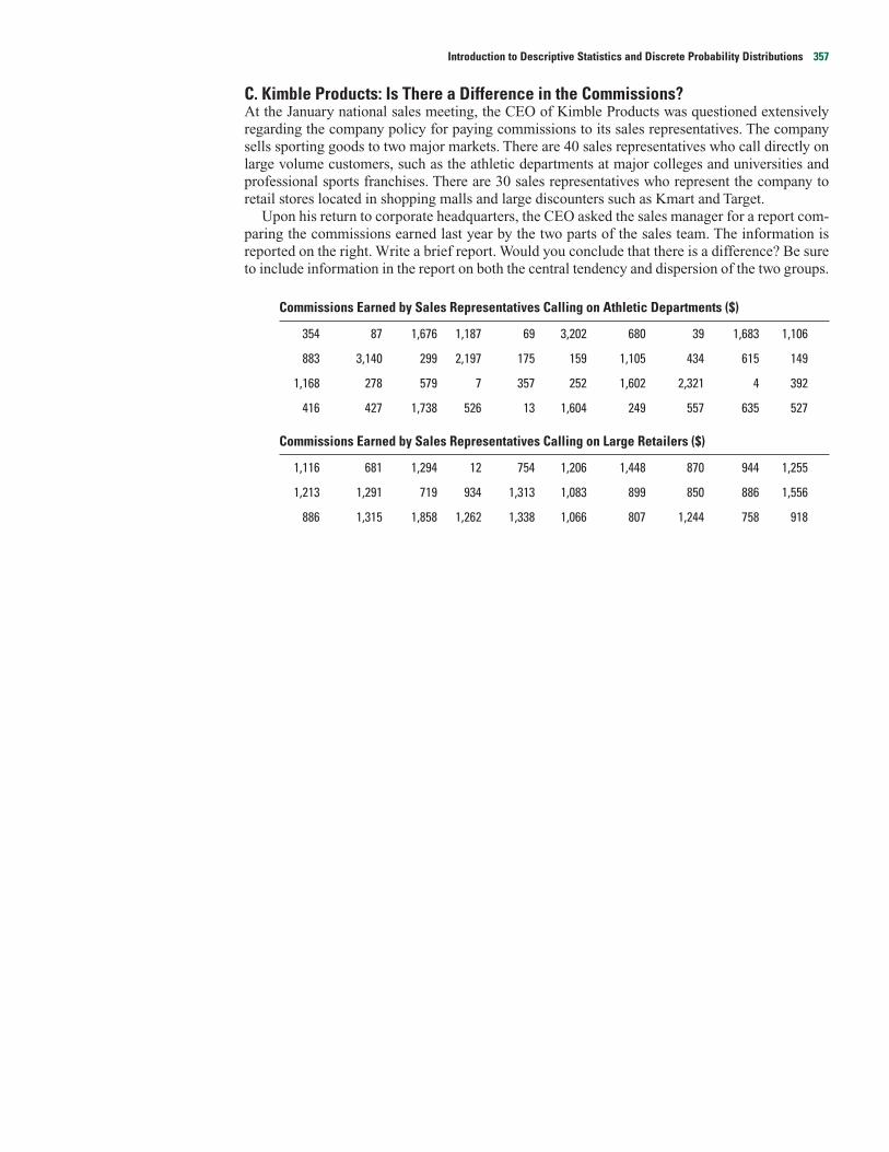
C. Kimble Products: Is There a Difference in the Commissions?At the January national sales meeting, the CEO of Kimble Products was questioned extensivelyregarding the company policy for paying commissions to its sales representatives. The companysells sporting goods to two major markets. There are 40 sales representatives who call directly onlarge volume customers, such as the athletic departments at major colleges and universities andprofessional sports franchises. There are 30 sales representatives who represent the company toretail stores located in shopping malls and large discounters such as Kmart and Target.
Upon his return to corporate headquarters, the CEO asked the sales manager for a report com-paring the commissions earned last year by the two parts of the sales team. The information isreported on the right. Write a brief report. Would you conclude that there is a difference? Be sureto include information in the report on both the central tendency and dispersion of the two groups.
Commissions Earned by Sales Representatives Calling on Athletic Departments ($)
354 87 1,676 1,187 69 3,202 680 39 1,683 1,106
883 3,140 299 2,197 175 159 1,105 434 615 149
1,168 278 579 7 357 252 1,602 2,321 4 392
416 427 1,738 526 13 1,604 249 557 635 527
Commissions Earned by Sales Representatives Calling on Large Retailers ($)
1,116 681 1,294 12 754 1,206 1,448 870 944 1,255
1,213 1,291 719 934 1,313 1,083 899 850 886 1,556
886 1,315 1,858 1,262 1,338 1,066 807 1,244 758 918
Introduction to Descriptive Statistics and Discrete Probability Distributions 357
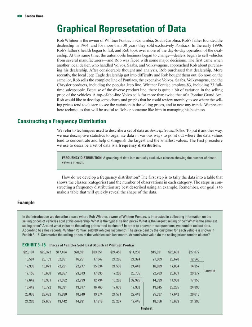
358 Section Three
Graphical Represetation of DataRob Whitner is the owner of Whitner Pontiac in Columbia, South Carolina. Rob’s father founded thedealership in 1964, and for more than 30 years they sold exclusively Pontiacs. In the early 1990sRob’s father’s health began to fail, and Rob took over more of the day-to-day operation of the deal-ership. At this same time, the automobile business began to change—dealers began to sell vehiclesfrom several manufacturers—and Rob was faced with some major decisions. The first came whenanother local dealer, who handled Volvos, Saabs, and Volkswagens, approached Rob about purchas-ing his dealership. After considerable thought and analysis, Rob purchased that dealership. Morerecently, the local Jeep Eagle dealership got into difficulty and Rob bought them out. So now, on thesame lot, Rob sells the complete line of Pontiacs, the expensive Volvos, Saabs, Volkswagens, and theChrysler products, including the popular Jeep line. Whitner Pontiac employs 83, including 23 full-time salespeople. Because of the diverse product line, there is quite a bit of variation in the sellingprice of the vehicles. A top-of-the-line Volvo sells for more than twice that of a Pontiac Grand Am.Rob would like to develop some charts and graphs that he could review monthly to see where the sell-ing prices tend to cluster, to see the variation in the selling prices, and to note any trends. We presenthere techniques that will be useful to Rob or someone like him in managing his business.
Constructing a Frequency DistributionWe refer to techniques used to describe a set of data as descriptive statistics. To put it another way,we use descriptive statistics to organize data in various ways to point out where the data valuestend to concentrate and help distinguish the largest and the smallest values. The first procedurewe use to describe a set of data is a frequency distribution.
How do we develop a frequency distribution? The first step is to tally the data into a table thatshows the classes (categories) and the number of observations in each category. The steps in con-structing a frequency distribution are best described using an example. Remember, our goal is tomake a table that will quickly reveal the shape of the data.
Example
In the Introduction we describe a case where Rob Whitner, owner of Whitner Pontiac, is interested in collecting information on theselling prices of vehicles sold at his dealership. What is the typical selling price? What is the largest selling price? What is the smallestselling price? Around what value do the selling prices tend to cluster? In order to answer these questions, we need to collect data.According to sales records, Whitner Pontiac sold 80 vehicles last month. The price paid by the customer for each vehicle is shown inExhibit 3–18. Summarize the selling prices of the vehicles sold last month. Around what value do the selling prices tend to cluster?
EXHIBIT 3–18 Prices of Vehicles Sold Last Month at Whitner Pontiac
$20,197 $20,372 $17,454 $20,591 $23,651 $24,453 $14,266 $15,021 $25,683 $27,872
16,587 20,169 32,851 16,251 17,047 21,285 21,324 21,609 25,670 12,546
12,935 16,873 22,251 22,277 25,034 21,533 24,443 16,889 17,004 14,357
17,155 16,688 20,657 23,613 17,895 17,203 20,765 22,783 23,661 29,277Lowest
17,642 18,981 21,052 22,799 12,794 15,263 32,925 14,399 14,968 17,356
18,442 18,722 16,331 19,817 16,766 17,633 17,962 19,845 23,285 24,896
26,076 29,492 15,890 18,740 19,374 21,571 22,449 25,337 17,642 20,613
21,220 27,655 19,442 14,891 17,818 23,237 17,445 18,556 18,639 21,296
Highest
FREQUENCY DISTRIBUTION A grouping of data into mutually exclusive classes showing the number of obser-vations in each.
358 Section Three358 Section Three

Introduction to Descriptive Statistics and Discrete Probability Distributions 359
Solution
We refer to the unorganized information in Exhibit 3–18 as raw data or ungrouped data. With a littlesearching, we can find the lowest selling price ($12,546) and the highest selling price ($32,925), but that isabout all. It is difficult to determine a typical selling price. It is also difficult to visualize where the sellingprices tend to occur. The raw data are more easily interpreted if organized into a frequency distribution.
STEP 1: Decide on the number of classes. The goal is to use just enough groupings or classes to reveal theshape of the distribution. Some judgment is needed here. Too many classes or too few classesmight not reveal the basic shape of the set of data. In the vehicle selling price problem, for exam-ple, three classes would not give much insight into the pattern of the data (see Exhibit 3–19).
EXHIBIT 3–19 An Example of Too Few Classes
Number ofVehicle Selling Price ($) Vehicles
12,000 up to 21,000 48
21,000 up to 30,000 30
30,000 up to 39,000 2
Total 80
A useful recipe to determine the number of classes is the “2 to the k rule.” This guide suggests youselect the smallest number (k) for the number of classes such that 2k (in words, 2 raised to the power ofk) is greater than the number of observations (n).
In the Whitner Pontiac example, there were 80 vehicles sold. So n � 80. If we try k � 6, which meanswe would use 6 classes, then 26 � 64, somewhat less than 80. Hence, 6 is not enough classes. If we let k� 7, then 27 � 128, which is greater than 80. So the recommended number of classes is 7.
STEP 2: Determine the class interval or width. Generally the class interval or width should be the samefor all classes. The classes all taken together must cover at least the distance from the lowestvalue in the raw data up to the highest value. Expressing these words in a formula:
i �H � L
k
where i is the class interval, H is the highest observed value, L is the lowest observed value, and k is thenumber of classes.
In the Whitner Pontiac case, the lowest value is $12,546 and the highest value is $32,925. If we need 7classes, the interval should be at least ($32,925�$12,546)/7 � $2,911. In practice this interval size is usu-ally rounded up to some convenient number, such as a multiple of 10 or 100. The value of $3,000 mightreadily be used in this case.
Unequal class intervals present problems in graphically portraying the distribution and in doing someof the computations. Unequal class intervals, however, may be necessary in certain situations to avoid alarge number of empty, or almost empty, classes. Such is the case in Exhibit 3–20. The Internal RevenueService used unequal-sized class intervals to report the adjusted gross income on individual tax returns.Had they used an equal-sized interval of, say, $1,000, more than 1,000 classes would have been requiredto describe all the incomes. A frequency distribution with 1,000 classes would be difficult to interpret. Inthis case the distribution is easier to understand in spite of the unequal classes. Note also that the num-ber of income tax returns or “frequencies” is reported in thousands in this particular table. This alsomakes the information easier to understand.
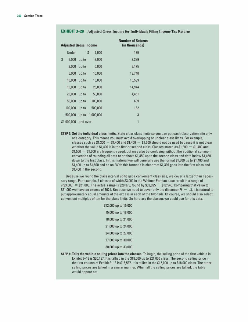
360 Section Three
EXHIBIT 3–20 Adjusted Gross Income for Individuals Filing Income Tax Returns
Number of ReturnsAdjusted Gross Income (in thousands)
Under $ 2,000 135
$ 2,000 up to 3,000 3,399
3,000 up to 5,000 8,175
5,000 up to 10,000 19,740
10,000 up to 15,000 15,539
15,000 up to 25,000 14,944
25,000 up to 50,000 4,451
50,000 up to 100,000 699
100,000 up to 500,000 162
500,000 up to 1,000,000 3
$1,000,000 and over 1
STEP 3: Set the individual class limits. State clear class limits so you can put each observation into onlyone category. This means you must avoid overlapping or unclear class limits. For example,classes such as $1,300 � $1,400 and $1,400 � $1,500 should not be used because it is not clearwhether the value $1,400 is in the first or second class. Classes stated as $1,300 � $1,400 and$1,500 � $1,600 are frequently used, but may also be confusing without the additional commonconvention of rounding all data at or above $1,450 up to the second class and data below $1,450down to the first class. In this material we will generally use the format $1,300 up to $1,400 and$1,400 up to $1,500 and so on. With this format it is clear that $1,399 goes into the first class and$1,400 in the second.
Because we round the class interval up to get a convenient class size, we cover a larger than neces-sary range. For example, 7 classes of width $3,000 in the Whitner Pontiac case result in a range of7($3,000) � $21,000. The actual range is $20,379, found by $32,925 � $12,546. Comparing that value to$21,000 we have an excess of $621. Because we need to cover only the distance (H � L), it is natural toput approximately equal amounts of the excess in each of the two tails. Of course, we should also selectconvenient multiples of ten for the class limits. So here are the classes we could use for this data.
$12,000 up to 15,000
15,000 up to 18,000
18,000 up to 21,000
21,000 up to 24,000
24,000 up to 27,000
27,000 up to 30,000
30,000 up to 33,000
STEP 4: Tally the vehicle selling prices into the classes. To begin, the selling price of the first vehicle inExhibit 3–18 is $20,197. It is tallied in the $18,000 up to $21,000 class. The second selling price inthe first column of Exhibit 3–18 is $16,587. It is tallied in the $15,000 up to $18,000 class. The otherselling prices are tallied in a similar manner. When all the selling prices are tallied, the tablewould appear as:
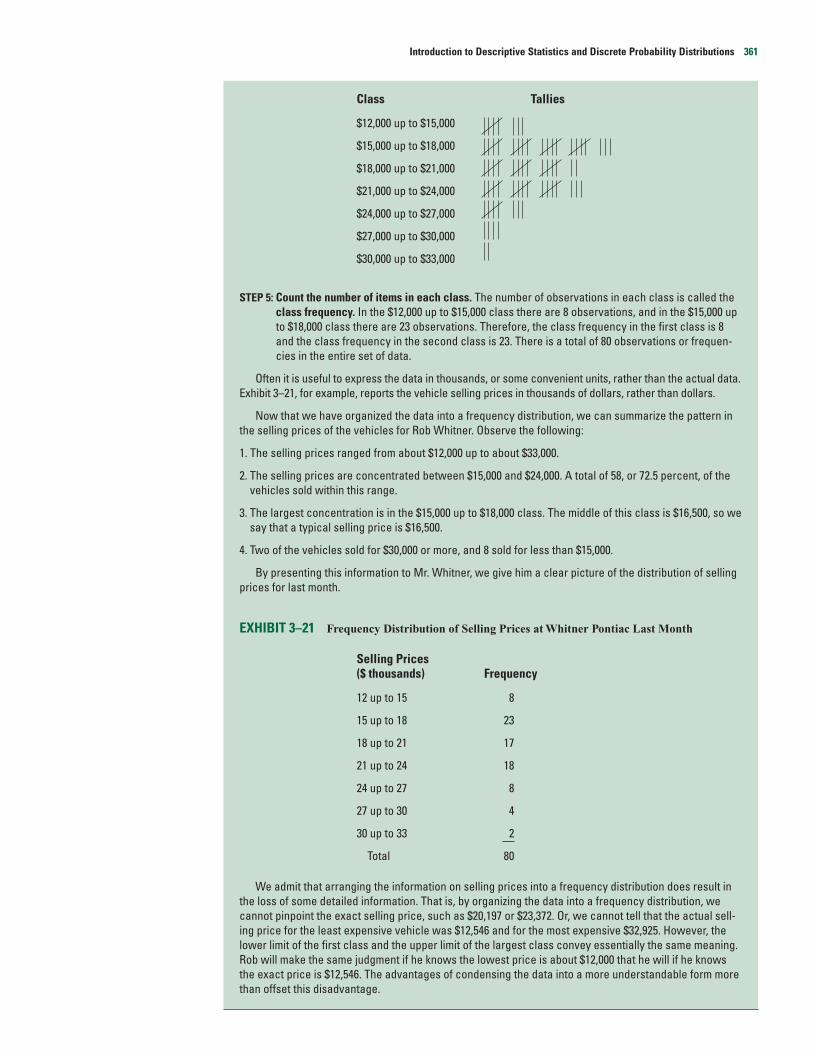
Introduction to Descriptive Statistics and Discrete Probability Distributions 361
Class Tallies
$12,000 up to $15,000
$15,000 up to $18,000
$18,000 up to $21,000
$21,000 up to $24,000
$24,000 up to $27,000
$27,000 up to $30,000
$30,000 up to $33,000
STEP 5: Count the number of items in each class. The number of observations in each class is called theclass frequency. In the $12,000 up to $15,000 class there are 8 observations, and in the $15,000 upto $18,000 class there are 23 observations. Therefore, the class frequency in the first class is 8and the class frequency in the second class is 23. There is a total of 80 observations or frequen-cies in the entire set of data.
Often it is useful to express the data in thousands, or some convenient units, rather than the actual data.Exhibit 3–21, for example, reports the vehicle selling prices in thousands of dollars, rather than dollars.
Now that we have organized the data into a frequency distribution, we can summarize the pattern inthe selling prices of the vehicles for Rob Whitner. Observe the following:
1. The selling prices ranged from about $12,000 up to about $33,000.
2. The selling prices are concentrated between $15,000 and $24,000. A total of 58, or 72.5 percent, of thevehicles sold within this range.
3. The largest concentration is in the $15,000 up to $18,000 class. The middle of this class is $16,500, so wesay that a typical selling price is $16,500.
4. Two of the vehicles sold for $30,000 or more, and 8 sold for less than $15,000.
By presenting this information to Mr. Whitner, we give him a clear picture of the distribution of sellingprices for last month.
EXHIBIT 3–21 Frequency Distribution of Selling Prices at Whitner Pontiac Last Month
Selling Prices($ thousands) Frequency
12 up to 15 8
15 up to 18 23
18 up to 21 17
21 up to 24 18
24 up to 27 8
27 up to 30 4
30 up to 33 2
Total 80
We admit that arranging the information on selling prices into a frequency distribution does result inthe loss of some detailed information. That is, by organizing the data into a frequency distribution, wecannot pinpoint the exact selling price, such as $20,197 or $23,372. Or, we cannot tell that the actual sell-ing price for the least expensive vehicle was $12,546 and for the most expensive $32,925. However, thelower limit of the first class and the upper limit of the largest class convey essentially the same meaning.Rob will make the same judgment if he knows the lowest price is about $12,000 that he will if he knowsthe exact price is $12,546. The advantages of condensing the data into a more understandable form morethan offset this disadvantage.

Snapshot 3–6In 1788, James Madison, John Jay, and Alexander Hamilton anonymously published a series of essays entitled The Federalist. These Federalistpapers were an attempt to convince the people of New York that they should ratify the Constitution. In the course of history, the authorship of mostof these papers became known, but 12 remained contested. Through the use of statistical analysis, and particularly the study of the frequency of theuse of various words, we can now conclude that James Madison is the likely author of the 12 papers. In fact, the statistical evidence that Madisonis the author is overwhelming.
Self-Review 3–17
Class Intervals and Class Midpoints
We will use two other terms frequently: class midpoint and class interval. The midpoint, alsocalled the class mark, is halfway between the lower limits of two consecutive classes. It can becomputed by adding the lower class limit to the upper class limit and dividing by 2. Referring toExhibit 3–21, for the first class the lower class limit is $12,000 and the next limit is $15,000. Theclass midpoint is $13,500, found by ($12,000 � $15,000)/2. The midpoint of $13,500 best rep-resents, or is typical of, the selling price of the vehicles in that class.
To determine the class interval, subtract the lower limit of the class from the lower limit of thenext class. The class interval of the vehicle selling price data is $3,000, which we find by sub-tracting the lower limit of the first class, $12,000, from the lower limit of the next class; that is,$15,000 � $12,000 � $3,000. You can also determine the class interval by finding the differencebetween consecutive midpoints. The midpoint of the first class is $13,500 and the midpoint of thesecond class is $16,500. The difference is $3,000.
A Computer Example
There are many software packages that perform statistical calculations and output the results.Throughout this material we will show the output from Microsoft Excel; from MegaStat, whichis an add-in to Microsoft Excel; and from MINITAB. The commands necessary to generate theoutputs are given in the Computer Commands section’s.
The commissions earned for the first quarter of last year by the eleven members of the sales staff atMaster Chemical Company are:
$1,650 $1,475 $1,510 $1,670 $1,595 $1,760 $1,540 $1,495 $1,590 $1,625 $1,510
(a) What are the values such as $1,650 and $1,475 called?
(b) Using $1,400 up to $1,500 as the first class, $1,500 up to $1,600 as the sec-ond class, and so forth, organize the quarterly commissions into a frequency distribution.
(c) What are the numbers in the right column of your frequency distribution called?
(d) Describe the distribution of monthly commissions, based on the frequency distribution. What is thelargest amount of commission earned? What is the smallest? What is the typical amount earned?
362 Section Three

Introduction to Descriptive Statistics and Discrete Probability Distributions 363
The following is a frequency distribution, produced by MegaStat, showing the prices of the 80vehicles sold last month at Whitner Pontiac. The form of the output is somewhat different than thefrequency distribution of Exhibit 3–20, but the overall conclusions are the same.
Self-Review 3–18
Relative Frequency DistributionIt may be desirable to convert class frequencies to relative class frequencies to show the fractionof the total number of observations in each class. In our vehicle sales example, we may want toknow what percent of the vehicle prices are in the $18,000 up to $21,000 class. In another study,we may want to know what percent of the employees are absent between one and three days peryear due to illness.
To convert a frequency distribution to a relative frequency distribution, each of the class fre-quencies is divided by the total number of observations. Using the distribution of vehicle salesagain (Exhibit 3–21, where the selling price is reported in thousands of dollars), the relative fre-quency for the $12,000 up to $15,000 class is 0.10, found by dividing 8 by 80. That is, the priceof 10 percent of the vehicles sold at Whitner Pontiac is between $12,000 and $15,000. The rela-tive frequencies for the remaining classes are shown in Exhibit 3–22.
During the 1998 baseball season, Mark McGuire broke the home run record by hitting 70 home runs. Thelongest was 550 feet and the shortest was 340 feet. It may also be interesting to note that the home runthat actually broke the record was “only” 341 feet. You need to construct a frequency distribution forthese home run lengths.
(a) How many classes would you use?
(b) How wide would you make the classes?
(c) What are the actual classes you would use?
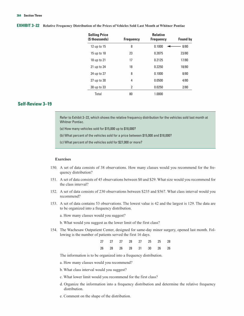
364 Section Three
EXHIBIT 3–22 Relative Frequency Distribution of the Prices of Vehicles Sold Last Month at Whitner Pontiac
Selling Price Relative($ thousands) Frequency Frequency Found by
12 up to 15 8 0.1000 8/80
15 up to 18 23 0.2875 23/80
18 up to 21 17 0.2125 17/80
21 up to 24 18 0.2250 18/80
24 up to 27 8 0.1000 8/80
27 up to 30 4 0.0500 4/80
30 up to 33 2 0.0250 2/80
Total 80 1.0000
Self-Review 3–19
Exercises
150. A set of data consists of 38 observations. How many classes would you recommend for the fre-quency distribution?
151. A set of data consists of 45 observations between $0 and $29. What size would you recommend forthe class interval?
152. A set of data consists of 230 observations between $235 and $567. What class interval would yourecommend?
153. A set of data contains 53 observations. The lowest value is 42 and the largest is 129. The data areto be organized into a frequency distribution.
a. How many classes would you suggest?
b. What would you suggest as the lower limit of the first class?
154. The Wachesaw Outpatient Center, designed for same-day minor surgery, opened last month. Fol-lowing is the number of patients served the first 16 days.
27 27 27 28 27 25 25 28
26 28 26 28 31 30 26 26
The information is to be organized into a frequency distribution.
a. How many classes would you recommend?
b. What class interval would you suggest?
c. What lower limit would you recommend for the first class?
d. Organize the information into a frequency distribution and determine the relative frequency distribution.
e. Comment on the shape of the distribution.
Refer to Exhibit 3–22, which shows the relative frequency distribution for the vehicles sold last month atWhitner Pontiac.
(a) How many vehicles sold for $15,000 up to $18,000?
(b) What percent of the vehicles sold for a price between $15,000 and $18,000?
(c) What percent of the vehicles sold for $27,000 or more?
155. The Quick Change Oil Company has a number of outlets in the metropolitan Seattle area. The num-bers of oil changes at the Oak Street outlet in the past 20 days are:
65 98 55 62 79 59 51 90 72 56
70 62 66 80 94 79 63 73 71 85
The data are to be organized into a frequency distribution.
a. How many classes would you recommend?
b. What class interval would you suggest?
c. What lower limit would you recommend for the first class?
d. Organize the number of oil changes into a frequency distribution.
e. Comment on the shape of the frequency distribution. Also determine the relative frequency dis-tribution.
156. The local manager of Food Queen is interested in the number of times a customer shops at her storeduring a two-week period. The responses of 51 customers were:
5 3 3 1 4 4 5 6 4 2 6 6 6 7 1
1 14 1 2 4 4 4 5 6 3 5 3 4 5 6
8 4 7 6 5 9 11 3 12 4 7 6 5 15 1
1 10 8 9 2 12
a. Starting with 0 as the lower limit of the first class and using a class interval of 3, organize the datainto a frequency distribution.
b. Describe the distribution. Where do the data tend to cluster?
c. Convert the distribution to a relative frequency distribution.
157. Moore Travel Agency, a nationwide travel agency, offers special rates on certain Caribbean cruises tosenior citizens. The president of Moore Travel wants additional information on the ages of those peo-ple taking cruises. A random sample of 40 customers taking a cruise last year revealed these ages.
77 18 63 84 38 54 50 59 54 56 36 26 50 34 44
41 58 58 53 51 62 43 52 53 63 62 62 65 61 52
60 60 45 66 83 71 63 58 61 71
a. Organize the data into a frequency distribution, using seven classes and 15 as the lower limit ofthe first class. What class interval did you select?
b. Where do the data tend to cluster?
c. Describe the distribution.
d. Determine the relative frequency distribution.
Stem-and-Leaf DisplaysWe showed how to organize data into a frequency distribution so we could summarize the rawdata into a meaningful form. The major advantage to organizing the data into a frequency distri-bution is that we get a quick visual picture of the shape of the distribution without doing any fur-ther calculation. That is, we can see where the data are concentrated and also determine whether
Introduction to Descriptive Statistics and Discrete Probability Distributions 365
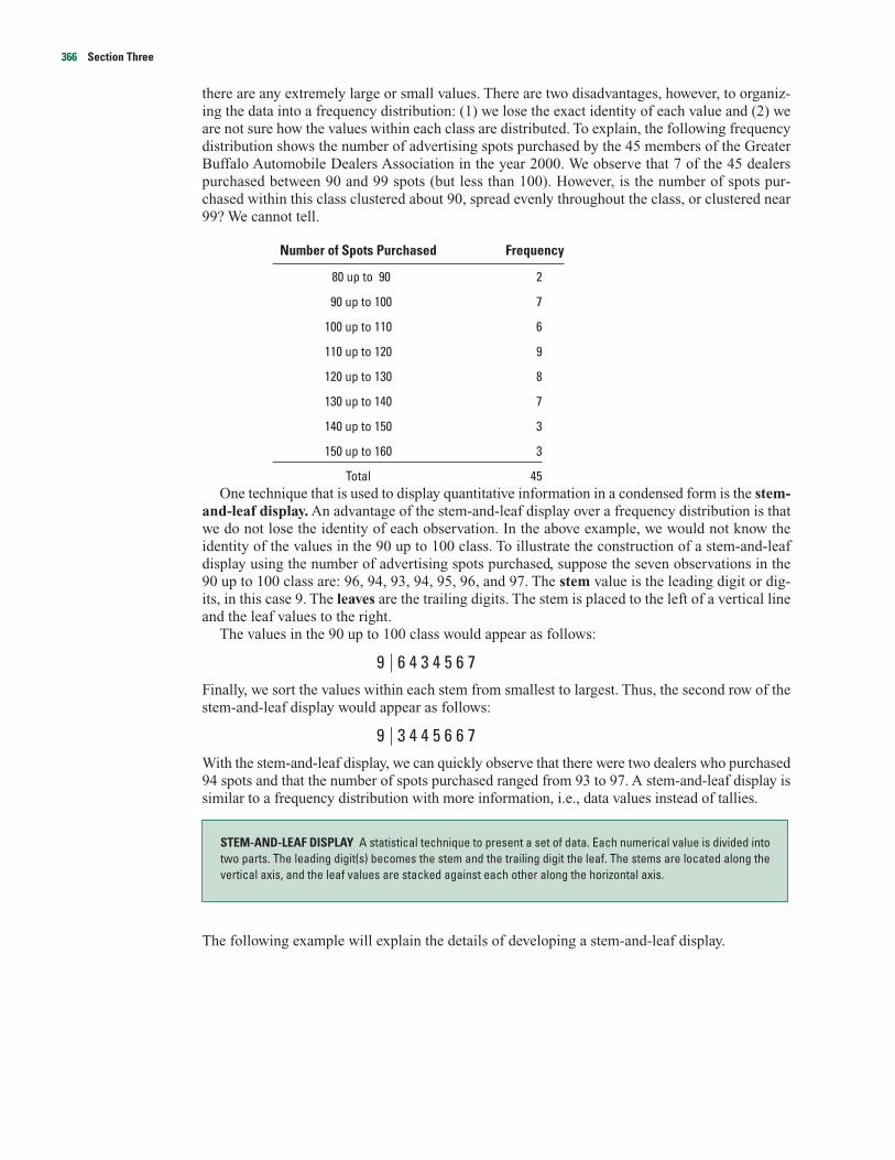
there are any extremely large or small values. There are two disadvantages, however, to organiz-ing the data into a frequency distribution: (1) we lose the exact identity of each value and (2) weare not sure how the values within each class are distributed. To explain, the following frequencydistribution shows the number of advertising spots purchased by the 45 members of the GreaterBuffalo Automobile Dealers Association in the year 2000. We observe that 7 of the 45 dealerspurchased between 90 and 99 spots (but less than 100). However, is the number of spots pur-chased within this class clustered about 90, spread evenly throughout the class, or clustered near99? We cannot tell.
Number of Spots Purchased Frequency
80 up to 90 2
90 up to 100 7
100 up to 110 6
110 up to 120 9
120 up to 130 8
130 up to 140 7
140 up to 150 3
150 up to 160 3
Total 45One technique that is used to display quantitative information in a condensed form is the stem-
and-leaf display. An advantage of the stem-and-leaf display over a frequency distribution is thatwe do not lose the identity of each observation. In the above example, we would not know theidentity of the values in the 90 up to 100 class. To illustrate the construction of a stem-and-leafdisplay using the number of advertising spots purchased, suppose the seven observations in the90 up to 100 class are: 96, 94, 93, 94, 95, 96, and 97. The stem value is the leading digit or dig-its, in this case 9. The leaves are the trailing digits. The stem is placed to the left of a vertical lineand the leaf values to the right.
The values in the 90 up to 100 class would appear as follows:
9 � 6 4 3 4 5 6 7Finally, we sort the values within each stem from smallest to largest. Thus, the second row of thestem-and-leaf display would appear as follows:
9 � 3 4 4 5 6 6 7With the stem-and-leaf display, we can quickly observe that there were two dealers who purchased94 spots and that the number of spots purchased ranged from 93 to 97. A stem-and-leaf display issimilar to a frequency distribution with more information, i.e., data values instead of tallies.
The following example will explain the details of developing a stem-and-leaf display.
STEM-AND-LEAF DISPLAY A statistical technique to present a set of data. Each numerical value is divided intotwo parts. The leading digit(s) becomes the stem and the trailing digit the leaf. The stems are located along thevertical axis, and the leaf values are stacked against each other along the horizontal axis.
366 Section Three

Introduction to Descriptive Statistics and Discrete Probability Distributions 367
Example
Solution
From the data in Exhibit 3–23 we note that the smallest number of spots purchased is 88. So we will makethe first stem value 8. The largest number is 156, so we will have the stem values begin at 8 and continueto 15. The first number in Exhibit 3–23 is 96, which will have a stem value of 9 and a leaf value of 6. Mov-ing across the top row, the second value is 93 and the third is 88. After the first 3 data values are consid-ered, your chart is as follows.
Stem Leaf
8 8
9 6 3
10
11
12
13
14
15
Organizing all the data, the stem-and-leaf chart looks as follows.
Stem Leaf
8 8 9
9 6 3 5 6 4 4 7
10 8 7 3 4 6 3
11 7 3 2 7 2 1 9 8 3
12 7 5 7 0 5 5 0 4
13 9 5 2 9 4 6 8
14 8 2 3
15 6 5 5
Listed in Exhibit 3–23 is the number of 30-second radio advertising spots purchased by each of the 45members of the Greater Buffalo Automobile Dealers Association last year. Organize the data into a stem-and-leaf display. Around what values do the number of advertising spots tend to cluster? What is thefewest number of spots purchased by a dealer? The largest number purchased?
EXHIBIT 3–23 Number of Advertising Spots Purchased by Members of the Greater Buffalo
Automobile Dealers Association
96 93 88 117 127 95 113 96 108 94 148 156139 142 94 107 125 155 155 103 112 127 117 120112 135 132 111 125 104 106 139 134 119 97 89118 136 125 143 120 103 113 124 138
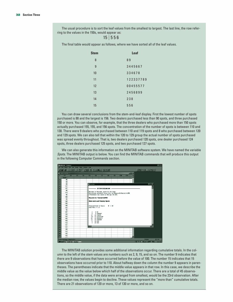
368 Section Three
The usual procedure is to sort the leaf values from the smallest to largest. The last line, the row refer-ring to the values in the 150s, would appear as:
15 � 5 5 6The final table would appear as follows, where we have sorted all of the leaf values.
Stem Leaf
8 8 9
9 3 4 4 5 6 6 7
10 3 3 4 6 7 8
11 1 2 2 3 3 7 7 8 9
12 0 0 4 5 5 5 7 7
13 2 4 5 6 8 9 9
14 2 3 8
15 5 5 6
You can draw several conclusions from the stem-and-leaf display. First the lowest number of spotspurchased is 88 and the largest is 156. Two dealers purchased less than 90 spots, and three purchased150 or more. You can observe, for example, that the three dealers who purchased more than 150 spotsactually purchased 155, 155, and 156 spots. The concentration of the number of spots is between 110 and130. There were 9 dealers who purchased between 110 and 119 spots and 8 who purchased between 120and 129 spots. We can also tell that within the 120 to 129 group the actual number of spots purchasedwas spread evenly throughout. That is, two dealers purchased 120 spots, one dealer purchased 124spots, three dealers purchased 125 spots, and two purchased 127 spots.
We can also generate this information on the MINITAB software system. We have named the variableSpots. The MINITAB output is below. You can find the MINITAB commands that will produce this outputin the following Computer Commands section.
The MINITAB solution provides some additional information regarding cumulative totals. In the col-umn to the left of the stem values are numbers such as 2, 9, 15, and so on. The number 9 indicates thatthere are 9 observations that have occurred before the value of 100. The number 15 indicates that 15observations have occurred prior to 110. About halfway down the column the number 9 appears in paren-theses. The parentheses indicate that the middle value appears in that row. In this case, we describe themiddle value as the value below which half of the observations occur. There are a total of 45 observa-tions, so the middle value, if the data were arranged from smallest, would be the 23rd observation. Afterthe median row, the values begin to decline. These values represent the “more than” cumulative totals.There are 21 observations of 120 or more, 13 of 130 or more, and so on.
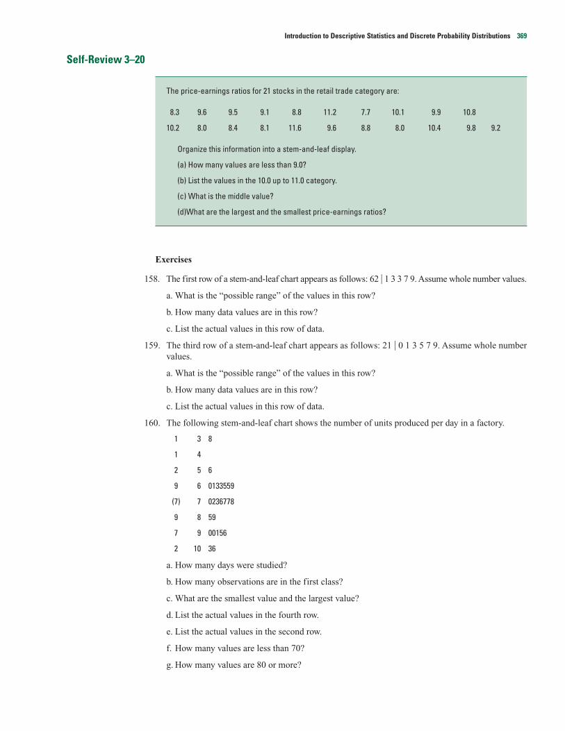
Self-Review 3–20
Exercises
158. The first row of a stem-and-leaf chart appears as follows: 62 � 1 3 3 7 9. Assume whole number values.
a. What is the “possible range” of the values in this row?
b. How many data values are in this row?
c. List the actual values in this row of data.
159. The third row of a stem-and-leaf chart appears as follows: 21 � 0 1 3 5 7 9. Assume whole numbervalues.
a. What is the “possible range” of the values in this row?
b. How many data values are in this row?
c. List the actual values in this row of data.
160. The following stem-and-leaf chart shows the number of units produced per day in a factory.
1 3 8
1 4
2 5 6
9 6 0133559
(7) 7 0236778
9 8 59
7 9 00156
2 10 36
a. How many days were studied?
b. How many observations are in the first class?
c. What are the smallest value and the largest value?
d. List the actual values in the fourth row.
e. List the actual values in the second row.
f. How many values are less than 70?
g. How many values are 80 or more?
The price-earnings ratios for 21 stocks in the retail trade category are:
8.3 9.6 9.5 9.1 8.8 11.2 7.7 10.1 9.9 10.8
10.2 8.0 8.4 8.1 11.6 9.6 8.8 8.0 10.4 9.8 9.2
Organize this information into a stem-and-leaf display.
(a) How many values are less than 9.0?
(b) List the values in the 10.0 up to 11.0 category.
(c) What is the middle value?
(d)What are the largest and the smallest price-earnings ratios?
Introduction to Descriptive Statistics and Discrete Probability Distributions 369

370 Section Three
h. What is the middle value?
i. How many values are between 60 and 89, inclusive?
161. The following stem-and-leaf chart reports the number of movies rented per day at Video Connection.
3 12 689
6 13 123
10 14 6889
13 15 589
15 16 35
20 17 24568
23 18 268
(5) 19 13456
22 20 034679
16 21 2239
12 22 789
9 23 00179
4 24 8
3 25 13
1 26
1 27 0
a. How many days were studied?
b. How many observations are in the last class?
c. What are the largest and the smallest values in the entire set of data?
d. List the actual values in the fourth row.
e. List the actual values in the next to the last row.
f. On how many days were less than 160 movies rented?
g. On how many days were 220 or more movies rented?
h. What is the middle value?
i. On how many days were between 170 and 210 movies rented?
162. A survey of the number of calls received by a sample of Southern Phone Company subscribers lastweek revealed the following information. Develop a stem-and-leaf chart. How many calls did atypical subscriber receive? What were the largest and the smallest number of calls received?
52 43 30 38 30 42 12 46 39
37 34 46 32 18 41 5
163. Aloha Banking Co. is studying the number of times their automatic teller, located in LoblawsSupermarket, is used each day. The following is the number of times it was used during each of thelast 30 days. Develop a stem-and-leaf chart. Summarize the data on the number of times the auto-matic teller was used: How many times was the teller used on a typical day? What were the largestand the smallest number of times the teller was used? Around what values did the number of timesthe teller was used tend to cluster?
83 64 84 76 84 54 75 59 70 61
63 80 84 73 68 52 65 90 52 77
95 36 78 61 59 84 95 47 87 60
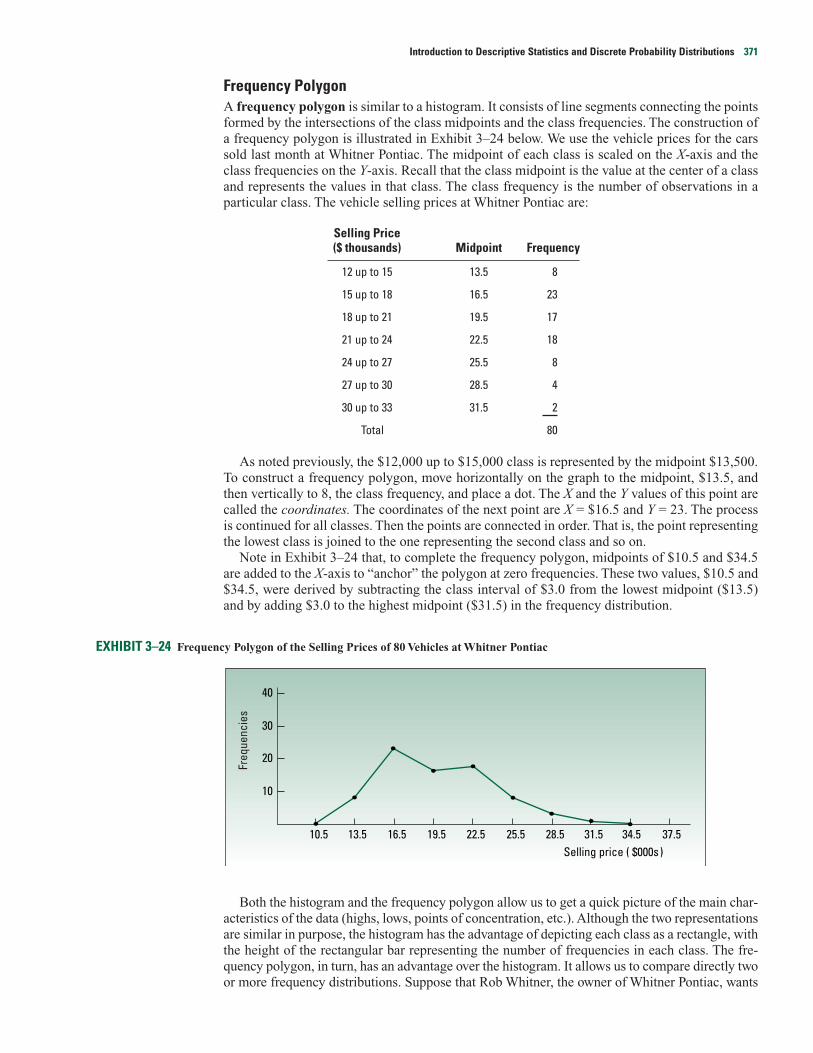
Introduction to Descriptive Statistics and Discrete Probability Distributions 371
Frequency PolygonA frequency polygon is similar to a histogram. It consists of line segments connecting the pointsformed by the intersections of the class midpoints and the class frequencies. The construction ofa frequency polygon is illustrated in Exhibit 3–24 below. We use the vehicle prices for the carssold last month at Whitner Pontiac. The midpoint of each class is scaled on the X-axis and theclass frequencies on the Y-axis. Recall that the class midpoint is the value at the center of a classand represents the values in that class. The class frequency is the number of observations in aparticular class. The vehicle selling prices at Whitner Pontiac are:
Selling Price($ thousands) Midpoint Frequency
12 up to 15 13.5 8
15 up to 18 16.5 23
18 up to 21 19.5 17
21 up to 24 22.5 18
24 up to 27 25.5 8
27 up to 30 28.5 4
30 up to 33 31.5 2
Total 80
As noted previously, the $12,000 up to $15,000 class is represented by the midpoint $13,500.To construct a frequency polygon, move horizontally on the graph to the midpoint, $13.5, andthen vertically to 8, the class frequency, and place a dot. The X and the Y values of this point arecalled the coordinates. The coordinates of the next point are X = $16.5 and Y = 23. The processis continued for all classes. Then the points are connected in order. That is, the point representingthe lowest class is joined to the one representing the second class and so on.
Note in Exhibit 3–24 that, to complete the frequency polygon, midpoints of $10.5 and $34.5are added to the X-axis to “anchor” the polygon at zero frequencies. These two values, $10.5 and$34.5, were derived by subtracting the class interval of $3.0 from the lowest midpoint ($13.5)and by adding $3.0 to the highest midpoint ($31.5) in the frequency distribution.
EXHIBIT 3–24 Frequency Polygon of the Selling Prices of 80 Vehicles at Whitner Pontiac
Both the histogram and the frequency polygon allow us to get a quick picture of the main char-acteristics of the data (highs, lows, points of concentration, etc.). Although the two representationsare similar in purpose, the histogram has the advantage of depicting each class as a rectangle, withthe height of the rectangular bar representing the number of frequencies in each class. The fre-quency polygon, in turn, has an advantage over the histogram. It allows us to compare directly twoor more frequency distributions. Suppose that Rob Whitner, the owner of Whitner Pontiac, wants
10
10.5
20
30
40
13.5 16.5 19.5 22.5 25.5 28.5 31.5Selling price ( $000s)
34.5 37.5
Freq
uenc
ies
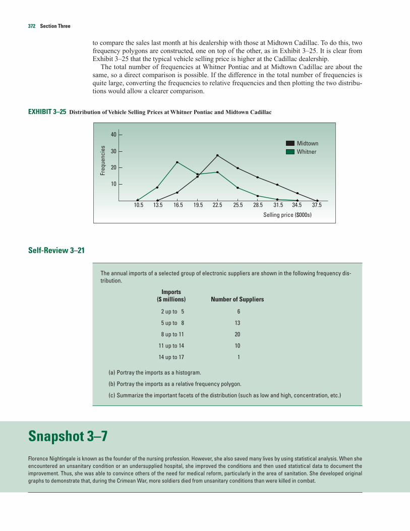
372 Section Three
to compare the sales last month at his dealership with those at Midtown Cadillac. To do this, twofrequency polygons are constructed, one on top of the other, as in Exhibit 3–25. It is clear fromExhibit 3–25 that the typical vehicle selling price is higher at the Cadillac dealership.
The total number of frequencies at Whitner Pontiac and at Midtown Cadillac are about thesame, so a direct comparison is possible. If the difference in the total number of frequencies isquite large, converting the frequencies to relative frequencies and then plotting the two distribu-tions would allow a clearer comparison.
EXHIBIT 3–25 Distribution of Vehicle Selling Prices at Whitner Pontiac and Midtown Cadillac
Self-Review 3–21
Snapshot 3–7Florence Nightingale is known as the founder of the nursing profession. However, she also saved many lives by using statistical analysis. When sheencountered an unsanitary condition or an undersupplied hospital, she improved the conditions and then used statistical data to document theimprovement. Thus, she was able to convince others of the need for medical reform, particularly in the area of sanitation. She developed originalgraphs to demonstrate that, during the Crimean War, more soldiers died from unsanitary conditions than were killed in combat.
The annual imports of a selected group of electronic suppliers are shown in the following frequency dis-tribution.
Imports($ millions) Number of Suppliers
2 up to 5 6
5 up to 8 13
8 up to 11 20
11 up to 14 10
14 up to 17 1
(a) Portray the imports as a histogram.
(b) Portray the imports as a relative frequency polygon.
(c) Summarize the important facets of the distribution (such as low and high, concentration, etc.)
40
30
20
10
10.5 13.5 16.5 19.5 22.5 25.5
Selling price ($000s)
Freq
uenc
ies
28.5 31.5
Midtown
34.5 37.5
Whitner
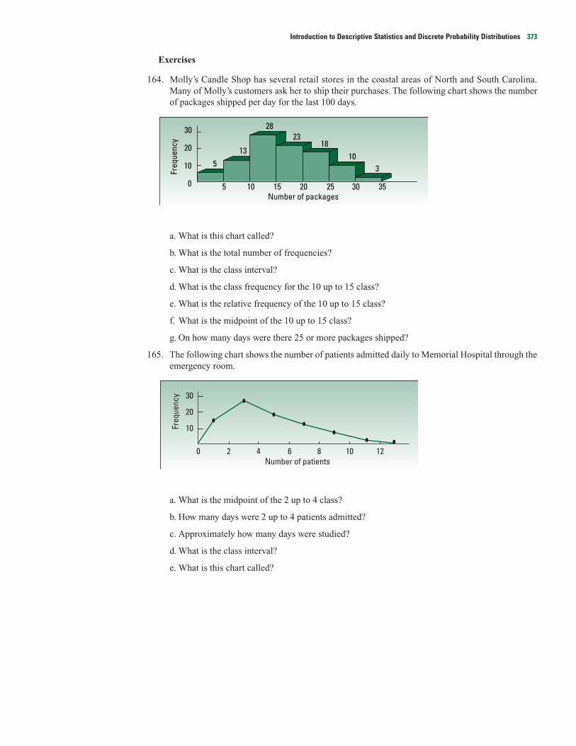
Introduction to Descriptive Statistics and Discrete Probability Distributions 373
Exercises
164. Molly’s Candle Shop has several retail stores in the coastal areas of North and South Carolina.Many of Molly’s customers ask her to ship their purchases. The following chart shows the numberof packages shipped per day for the last 100 days.
a. What is this chart called?
b. What is the total number of frequencies?
c. What is the class interval?
d. What is the class frequency for the 10 up to 15 class?
e. What is the relative frequency of the 10 up to 15 class?
f. What is the midpoint of the 10 up to 15 class?
g. On how many days were there 25 or more packages shipped?
165. The following chart shows the number of patients admitted daily to Memorial Hospital through theemergency room.
a. What is the midpoint of the 2 up to 4 class?
b. How many days were 2 up to 4 patients admitted?
c. Approximately how many days were studied?
d. What is the class interval?
e. What is this chart called?
0
10
20
30
2 4 6 8 10 12
Freq
uenc
y
Number of patients
Freq
uenc
y
Number of packages
10
0 5 10 15 20 25 30 35
20
30
13
2823
1810
35
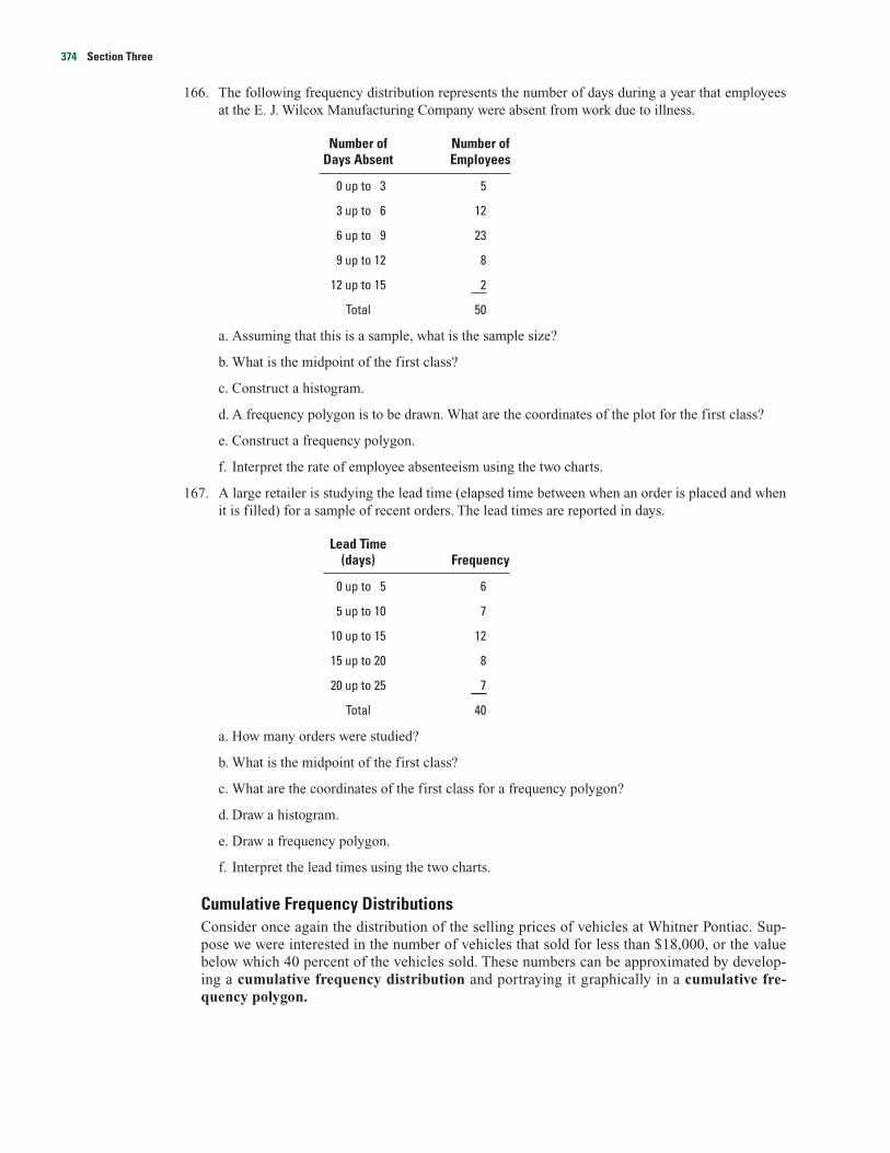
374 Section Three
166. The following frequency distribution represents the number of days during a year that employeesat the E. J. Wilcox Manufacturing Company were absent from work due to illness.
Number of Number ofDays Absent Employees
0 up to 3 5
3 up to 6 12
6 up to 9 23
9 up to 12 8
12 up to 15 2
Total 50
a. Assuming that this is a sample, what is the sample size?
b. What is the midpoint of the first class?
c. Construct a histogram.
d. A frequency polygon is to be drawn. What are the coordinates of the plot for the first class?
e. Construct a frequency polygon.
f. Interpret the rate of employee absenteeism using the two charts.
167. A large retailer is studying the lead time (elapsed time between when an order is placed and whenit is filled) for a sample of recent orders. The lead times are reported in days.
Lead Time(days) Frequency
0 up to 5 6
5 up to 10 7
10 up to 15 12
15 up to 20 8
20 up to 25 7
Total 40
a. How many orders were studied?
b. What is the midpoint of the first class?
c. What are the coordinates of the first class for a frequency polygon?
d. Draw a histogram.
e. Draw a frequency polygon.
f. Interpret the lead times using the two charts.
Cumulative Frequency DistributionsConsider once again the distribution of the selling prices of vehicles at Whitner Pontiac. Sup-pose we were interested in the number of vehicles that sold for less than $18,000, or the valuebelow which 40 percent of the vehicles sold. These numbers can be approximated by develop-ing a cumulative frequency distribution and portraying it graphically in a cumulative fre-quency polygon.

Introduction to Descriptive Statistics and Discrete Probability Distributions 375
Example
Solution
As the name implies, a cumulative frequency distribution and a cumulative frequency polygon requirecumulative frequencies. To construct a cumulative frequency distribution, refer to the preceding tableand note that there were eight vehicles sold for less than $15,000. Those 8 vehicles, plus the 23 in thenext higher class, for a total of 31, were sold for less than $18,000. The cumulative frequency for the nexthigher class is 48, found by 8 � 23 � 17. This process is continued for all the classes. All the vehicleswere sold for less than $33,000. (See Exhibit 3–26.)
EXHIBIT 3–26 Cumulative Frequency Distribution for Vehicle Selling Price
Selling Price($ thousands) Frequency Cumulative Frequency Found by
12 up to 15 8 8
15 up to 18 23 31 8 � 23
18 up to 21 17 48 8 � 23 � 17
21 up to 24 18 66 8 � 23 � 17 � 18
24 up to 27 8 74
27 up to 30 4 78
30 up to 33 2 80
Total 80
To plot a cumulative frequency distribution, scale the upper limit of each class along the X-axis andthe corresponding cumulative frequencies along the Y-axis. To provide additional information, you canlabel the vertical axis on the left in units and the vertical axis on the right in percent. In the Whitner Pon-tiac example, the vertical axis on the left is labeled from 0 to 80 and on the right from 0 to 100 percent.The value of 50 percent corresponds to 40 vehicles sold.
To begin the plotting, 8 vehicles sold for less than $15,000, so the first plot is at X � 15 and Y � 8. Thecoordinates for the next plot are X � 18 and Y � 31. The rest of the points are plotted and then the dotsconnected to form the chart (see Exhibit 3–27). To find the selling price below which half the cars sold,we draw a line from the 50 percent mark on the right-hand vertical axis over to the polygon, then drop
The frequency distribution of the vehicle selling prices at Whitner Pontiac is repeated from Exhibit 3–21.
Selling Price ($ thousands) Frequency
12 up to 15 8
15 up to 18 23
18 up to 21 17
21 up to 24 18
24 up to 27 8
27 up to 30 4
30 up to 33 2
Total 80
Construct a cumulative frequency polygon. Fifty percent of the vehicles were sold for less than whatamount? Twenty-five of the vehicles were sold for less than what amount?

376 Section Three
down to the X-axis and read the selling price. The value on the X-axis is about 19.5, so we estimate that50 percent of the vehicles sold for less than $19,500.
EXHIBIT 3–27 Cumulative Frequency Distribution for Vehicle Selling Price
To find the price below which 25 of the vehicles sold, we locate the value of 25 on the left-hand verti-cal axis. Next, we draw a horizontal line from the value of 25 to the polygon, and then drop down to the X-axis and read the price. It is about 17.5, so we estimate that 25 of the vehicles sold for less than $17,500.We can also make estimates of the percent of vehicles that sold for less than a particular amount.To explain, suppose we want to estimate the percent of vehicles that sold for less than $25,500. We beginby locating the value of 25.5 on the X-axis, move vertically to the polygon, and then horizontally to the ver-tical axis on the right. The value is about 87 percent, so we conclude that 87 percent of the vehicles soldfor less than $25,500.
Self-Review 3–22
A sample of the hourly wages of 15 employees at Food City Supermarkets was organized into the follow-ing table.
Hourly Wages Number of Employees
$ 6 up to $ 8 3
8 up to 10 7
10 up to 12 4
12 up to 14 1
(a) What is the table called?
(b) Develop a cumulative frequency distribution and portray the distribution in a cumulative fre-quency polygon.
(c) Based on the cumulative frequency polygon, how many employees earn $9 an hour or less? Half ofthe employees earn an hourly wage of how much more? Four employees earn how much less?
12 15 18 21 24 27 30 33
Num
ber o
f veh
icle
s so
ld
Perc
ent o
f veh
icle
s so
ld
Selling price ($000)
80
70
60
50
40
30
20
10
100
75
50
25
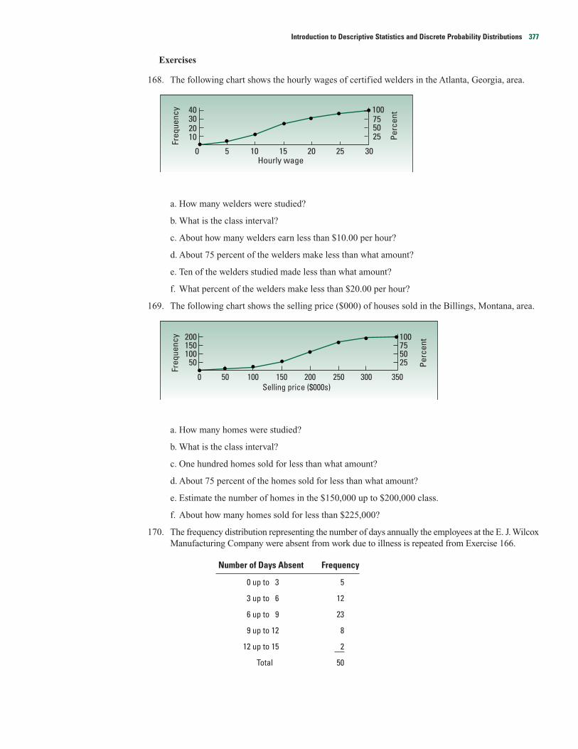
Exercises
168. The following chart shows the hourly wages of certified welders in the Atlanta, Georgia, area.
a. How many welders were studied?
b. What is the class interval?
c. About how many welders earn less than $10.00 per hour?
d. About 75 percent of the welders make less than what amount?
e. Ten of the welders studied made less than what amount?
f. What percent of the welders make less than $20.00 per hour?
169. The following chart shows the selling price ($000) of houses sold in the Billings, Montana, area.
a. How many homes were studied?
b. What is the class interval?
c. One hundred homes sold for less than what amount?
d. About 75 percent of the homes sold for less than what amount?
e. Estimate the number of homes in the $150,000 up to $200,000 class.
f. About how many homes sold for less than $225,000?
170. The frequency distribution representing the number of days annually the employees at the E. J. WilcoxManufacturing Company were absent from work due to illness is repeated from Exercise 166.
Number of Days Absent Frequency
0 up to 3 5
3 up to 6 12
6 up to 9 23
9 up to 12 8
12 up to 15 2
Total 50
Freq
uenc
y
Perc
ent200
150100
50
100 75 50 25
Selling price ($000s)500 100 150 200 250 350300
Freq
uenc
y
Hourly wage
Perc
ent
0 5 10 15 20 25 30
100755025
40302010
Introduction to Descriptive Statistics and Discrete Probability Distributions 377

378 Section Three
a. How many employees were absent less than three days annually? How many were absent lessthan six days due to illness?
b. Convert the frequency distribution to a cumulative frequency distribution.
c. Portray the cumulative distribution in the form of a cumulative frequency polygon.
d. Based on the cumulative frequency polygon, about three out of four employees were absent forhow many days or less due to illness?
171. The frequency distribution of the lead time to fill an order from Exercise 167 is repeated below.
Lead Time (days) Frequency
0 up to 5 6
5 up to 10 7
10 up to 15 12
15 up to 20 8
20 up to 25 7
Total 40
a. How many orders were filled in less than 10 days? In less than 15 days?
b. Convert the frequency distribution to a cumulative frequency distribution.
c. Develop a cumulative frequency polygon.
d. About 60 percent of the orders were filled in less than how many days?
Other Graphic Presentations of DataThe histogram, the frequency polygon, and the cumulative frequency polygon all have strongvisual appeal. That is, they are designed to capture the attention of the reader. In this section wewill examine some other graphical forms, namely the line chart, the bar chart, and the pie chart.These charts are seen extensively in USA Today, U.S. News and World Report, Business Week, andother newspapers, magazines, and government reports.
Exhibits 3–28 and 3–29 are examples of line charts. Line charts are particularly effective forbusiness because we can show the change in a variable over time. The variable, such as the num-ber of units sold or the total value of sales, is scaled along the vertical axis and time along the hor-izontal axis. Exhibit 3–28 shows the Dow Jones Industrial Average and the Nasdaq, the two mostwidely reported measures of business activity, on Tuesday, June 6, 2000. Both measures weredown for the day. The Dow closed at 10,735.57, down 79.73, and the Nasdaq at 3,756.39, down65.37, for the day.
EXHIBIT 3–28 Market Summary on June 6, 2000
10
DJIA
10,735.574:31 PM EST
The world’s coolest investment charting and research site.
major market indexes Launch RefreshIndexWatchWWW.BigCharts.com
@BigCharts.com
11 12 1 2 3
10,850
–79.73–0.74%
10,800
10,750
10,70010 11 12 1 2 3
3,900
3,850
3,800
3,750
3,700
NASDAQ
3,756.394:48 PM EST @BigCharts.com
–65.37–1.71%

Introduction to Descriptive Statistics and Discrete Probability Distributions 379
Exhibit 3–29 is also a line chart. It shows the circulation of the Sun Times newspaper begin-ning with 1995 through the year 2000. It shows the newspaper’s sales are increasing, but thegrowth rate of sales since 1997 seems to be slowing down.
EXHIBIT 3–29 The Sun Times Circulation from 1995 to 2000
Quite often two or more series of figures are plotted on the same line chart. Thus, one chart canshow the trend of several series. This allows for a comparison of several series over a period of time.Exhibit 3–30 shows the domestic and international sales (in millions of dollars) of Johnson andJohnson, Inc., for the years 1990 through 2000. We can easily see that the sales in both segments aregrowing, with the domestic component staying ahead of international sales in most years.
A bar chart can be used to depict any of the levels of measurement—nominal, ordinal, inter-val, or ratio. Suppose we want to show the difference in earnings based on the level of education.From the Census Bureau Current Population Reports, the average earnings for someone over theage of 18 are $22,895 if a high school diploma is the highest degree earned. With a bachelor’sdegree the average earnings increase to $40,478 and with a professional or master’s degree theamount increases to $73,165. This information is summarized in Exhibit 3–31. We call this charta horizontal bar chart because the bars are horizontal. With the chart it is easy to see that a per-son with a bachelor’s degree can expect to earn almost twice as much as someone with a highschool diploma. The expected earnings of someone with a master’s or professional degree isnearly twice that of a bachelor’s degree and more than three times that of high school.
EXHIBIT 3–30 Domestic and International Sales for Johnson and Johnson, Inc.
15,000
12,000
9,000
6,000
3,000'00
Year'97 '98'96'95'94'93'92'90 '91
International Domestic
Sale
s in
$ m
illio
ns
'99
800,000
600,000
400,000
200,000
0
Circ
ulat
ion
1998 1999 2000Year
199719961995
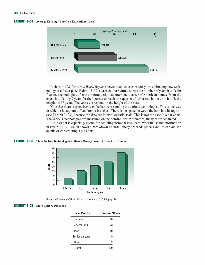
380 Section Three
EXHIBIT 3–31 Average Earnings Based on Educational Level
A chart in U.S. News and World Report showed that Americans today are embracing new tech-nology at a faster pace. Exhibit 3–32, a vertical bar chart, shows the number of years it took forfive key technologies, after their introduction, to enter one-quarter of American homes. From thechart, it took only 7 years for the Internet to reach one-quarter of American homes, but it took thetelephone 35 years. The years correspond to the height of the bars.
Note that there is space between the bars representing the various technologies. This is one wayin which a histogram differs from a bar chart. There is no space between the bars in a histogram(see Exhibit 3–23), because the data are interval or ratio scale. This is not the case in a bar chart.The various technologies are measured on the nominal scale; therefore, the bars are separated.
A pie chart is especially useful for depicting nominal level data. We will use the informationin Exhibit 3–33, which shows a breakdown of state lottery proceeds since 1964, to explain thedetails of constructing a pie chart.
EXHIBIT 3–32 Time for Key Technologies to Reach One-Quarter of American Homes
Source: US News and World Report. November 13, 2000, page 16.
EXHIBIT 3–33 State Lottery Proceeds
Use of Profits Percent Share
Education 56
General fund 23
Cities 10
Senior citizens 9
Other 2
Total 100
40
35
30
25
20
15
10
5
0Internet PCs Radio TV Phone
Technologies
Year
sH.S. Diploma
Bachelor's
Master's/Prof.
0 20 40 60 80Earnings ($ in thousands)
$73,165
$40,478
$22,895
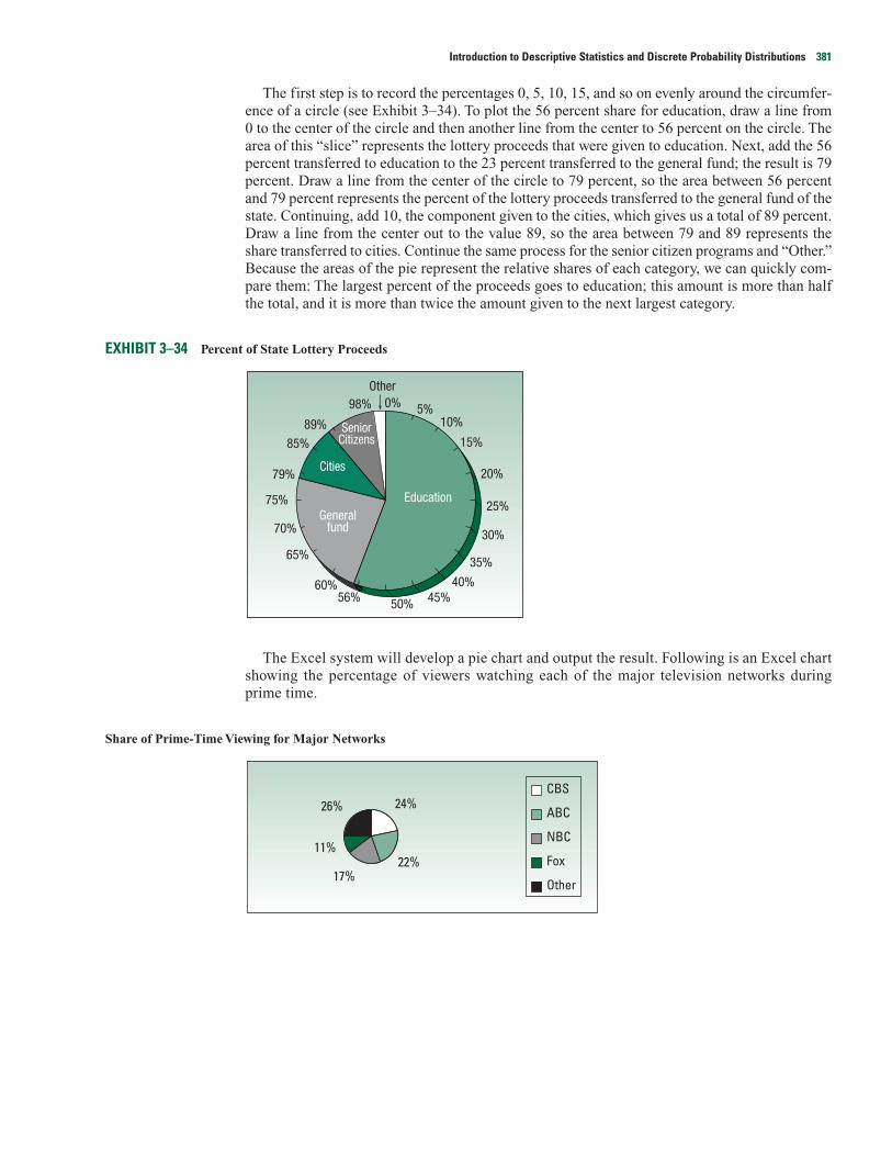
The first step is to record the percentages 0, 5, 10, 15, and so on evenly around the circumfer-ence of a circle (see Exhibit 3–34). To plot the 56 percent share for education, draw a line from0 to the center of the circle and then another line from the center to 56 percent on the circle. Thearea of this “slice” represents the lottery proceeds that were given to education. Next, add the 56percent transferred to education to the 23 percent transferred to the general fund; the result is 79percent. Draw a line from the center of the circle to 79 percent, so the area between 56 percentand 79 percent represents the percent of the lottery proceeds transferred to the general fund of thestate. Continuing, add 10, the component given to the cities, which gives us a total of 89 percent.Draw a line from the center out to the value 89, so the area between 79 and 89 represents theshare transferred to cities. Continue the same process for the senior citizen programs and “Other.”Because the areas of the pie represent the relative shares of each category, we can quickly com-pare them: The largest percent of the proceeds goes to education; this amount is more than halfthe total, and it is more than twice the amount given to the next largest category.
EXHIBIT 3–34 Percent of State Lottery Proceeds
The Excel system will develop a pie chart and output the result. Following is an Excel chartshowing the percentage of viewers watching each of the major television networks duringprime time.
Share of Prime-Time Viewing for Major Networks
CBS24%
22%17%
11%
26% ABC
NBC
Fox
Other
5%10%
15%
20%
25%
30%
35%
40%45%50%56%
60%
65%
70%
75%
79%
85%
89%
98% 0%
Generalfund
Cities
SeniorCitizens
Education
Other
Introduction to Descriptive Statistics and Discrete Probability Distributions 381
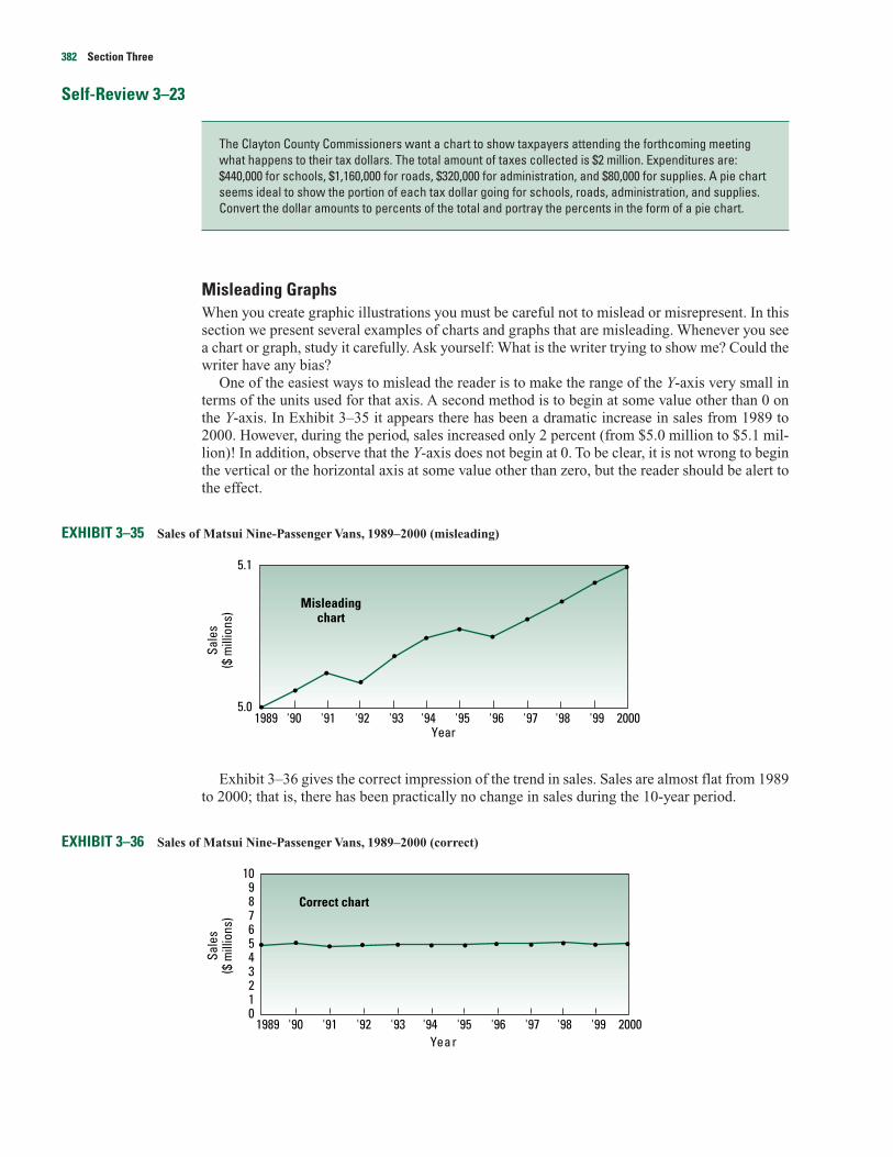
Self-Review 3–23
Misleading GraphsWhen you create graphic illustrations you must be careful not to mislead or misrepresent. In thissection we present several examples of charts and graphs that are misleading. Whenever you seea chart or graph, study it carefully. Ask yourself: What is the writer trying to show me? Could thewriter have any bias?
One of the easiest ways to mislead the reader is to make the range of the Y-axis very small interms of the units used for that axis. A second method is to begin at some value other than 0 onthe Y-axis. In Exhibit 3–35 it appears there has been a dramatic increase in sales from 1989 to2000. However, during the period, sales increased only 2 percent (from $5.0 million to $5.1 mil-lion)! In addition, observe that the Y-axis does not begin at 0. To be clear, it is not wrong to beginthe vertical or the horizontal axis at some value other than zero, but the reader should be alert tothe effect.
EXHIBIT 3–35 Sales of Matsui Nine-Passenger Vans, 1989–2000 (misleading)
Exhibit 3–36 gives the correct impression of the trend in sales. Sales are almost flat from 1989to 2000; that is, there has been practically no change in sales during the 10-year period.
EXHIBIT 3–36 Sales of Matsui Nine-Passenger Vans, 1989–2000 (correct)
109876543210 1989 2000 '90 '91 '92 '93 '94 '95 '96 '97 '98 '99
Sale
s($
mill
ions
)
Year
Correct chart
5.1
5.0
Misleadingchart
Sale
s($
mill
ions
)
Year 1989 2000 '90 '91 '92 '93 '94 '95 '96 '97 '98 '99
The Clayton County Commissioners want a chart to show taxpayers attending the forthcoming meetingwhat happens to their tax dollars. The total amount of taxes collected is $2 million. Expenditures are:$440,000 for schools, $1,160,000 for roads, $320,000 for administration, and $80,000 for supplies. A pie chartseems ideal to show the portion of each tax dollar going for schools, roads, administration, and supplies.Convert the dollar amounts to percents of the total and portray the percents in the form of a pie chart.
382 Section Three
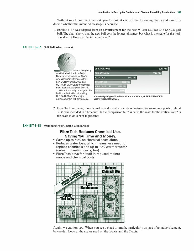
Introduction to Descriptive Statistics and Discrete Probability Distributions 383
Without much comment, we ask you to look at each of the following charts and carefullydecide whether the intended message is accurate.
1. Exhibit 3–37 was adapted from an advertisement for the new Wilson ULTRA DISTANCE golfball. The chart shows that the new ball gets the longest distance, but what is the scale for the hori-zontal axis? How was the test conducted?
EXHIBIT 3–37 Golf Ball Advertisement
2. Fibre Tech, in Largo, Florida, makes and installs fiberglass coatings for swimming pools. Exhibit3–38 was included in a brochure. Is the comparison fair? What is the scale for the vertical axis? Isthe scale in dollars or in percent?
EXHIBIT 3–38 Swimming Pool Coating Comparison
Fibre Tech Reduces Chemical Use,
Saving You Time and Money.• Saves up to 60% on chemical costs alone.• Reduces water loss, which means less need to
replace chemicals and up to 10% warmer water(reducing heating costs, too).
• Fibre Tech pays for itself in reduced mainte-nance and chemical costs.
Again, we caution you. When you see a chart or graph, particularly as part of an advertisement,be careful. Look at the scales used on the X-axis and the Y-axis.
ULTRA© DISTANCE
DUNLOP© DDH IV
MAXFLI MD©
TITLEIST© HVC
TOP-FLITE© Tour 90
TOP-FLITE© MAGNA
Combined yardage with a driver, #5 iron and #9 iron, ULTRA DISTANCE is clearly measurably longer.
Maybe everybody can't hit a ball like John Daly.But everybody wants to. That'swhy Wilson© is introducing the new ULTRA© DISTANCE ball.ULTRA DISTANCE is the longest,most accurate ball you'll ever hit. Wilson has totally redesigned this ball from the inside out, making ULTRA DISTANCE a major advancement in golf technology.
591.2 Yds.
584.6 Yds.
571.2 Yds.
569.3 Yds.
565.9 Yds.
564.3 Yds.
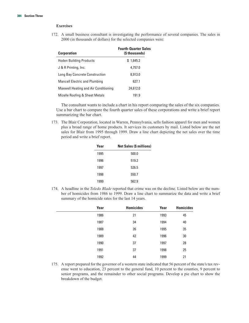
384 Section Three
Exercises
172. A small business consultant is investigating the performance of several companies. The sales in2000 (in thousands of dollars) for the selected companies were:
Fourth-Quarter SalesCorporation ($ thousands)
Hoden Building Products $ 1,645.2
J & R Printing, Inc. 4,757.0
Long Bay Concrete Construction 8,913.0
Mancell Electric and Plumbing 627.1
Maxwell Heating and Air Conditioning 24,612.0
Mizelle Roofing & Sheet Metals 191.9
The consultant wants to include a chart in his report comparing the sales of the six companies.Use a bar chart to compare the fourth quarter sales of these corporations and write a brief reportsummarizing the bar chart.
173. The Blair Corporation, located in Warren, Pennsylvania, sells fashion apparel for men and womenplus a broad range of home products. It services its customers by mail. Listed below are the netsales for Blair from 1995 through 1999. Draw a line chart depicting the net sales over the timeperiod and write a brief report.
Year Net Sales ($ millions)
1995 500.0
1996 519.2
1997 526.5
1998 550.7
1999 562.9
174. A headline in the Toledo Blade reported that crime was on the decline. Listed below are the num-ber of homicides from 1986 to 1999. Draw a line chart to summarize the data and write a briefsummary of the homicide rates for the last 14 years.
Year Homicides Year Homicides
1986 21 1993 45
1987 34 1994 40
1988 26 1995 35
1989 42 1996 30
1990 37 1997 28
1991 37 1998 25
1992 44 1999 21
175. A report prepared for the governor of a western state indicated that 56 percent of the state’s tax rev-enue went to education, 23 percent to the general fund, 10 percent to the counties, 9 percent tosenior programs, and the remainder to other social programs. Develop a pie chart to show thebreakdown of the budget.
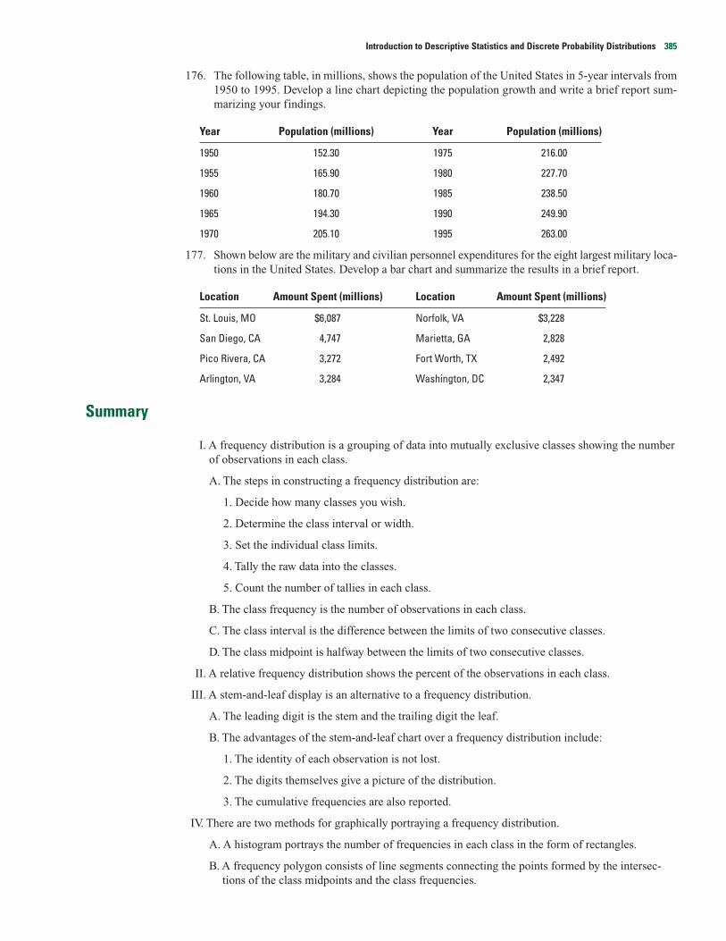
176. The following table, in millions, shows the population of the United States in 5-year intervals from1950 to 1995. Develop a line chart depicting the population growth and write a brief report sum-marizing your findings.
Year Population (millions) Year Population (millions)
1950 152.30 1975 216.00
1955 165.90 1980 227.70
1960 180.70 1985 238.50
1965 194.30 1990 249.90
1970 205.10 1995 263.00
177. Shown below are the military and civilian personnel expenditures for the eight largest military loca-tions in the United States. Develop a bar chart and summarize the results in a brief report.
Location Amount Spent (millions) Location Amount Spent (millions)
St. Louis, MO $6,087 Norfolk, VA $3,228
San Diego, CA 4,747 Marietta, GA 2,828
Pico Rivera, CA 3,272 Fort Worth, TX 2,492
Arlington, VA 3,284 Washington, DC 2,347
Summary
I. A frequency distribution is a grouping of data into mutually exclusive classes showing the numberof observations in each class.
A. The steps in constructing a frequency distribution are:
1. Decide how many classes you wish.
2. Determine the class interval or width.
3. Set the individual class limits.
4. Tally the raw data into the classes.
5. Count the number of tallies in each class.
B. The class frequency is the number of observations in each class.
C. The class interval is the difference between the limits of two consecutive classes.
D. The class midpoint is halfway between the limits of two consecutive classes.
II. A relative frequency distribution shows the percent of the observations in each class.
III. A stem-and-leaf display is an alternative to a frequency distribution.
A. The leading digit is the stem and the trailing digit the leaf.
B. The advantages of the stem-and-leaf chart over a frequency distribution include:
1. The identity of each observation is not lost.
2. The digits themselves give a picture of the distribution.
3. The cumulative frequencies are also reported.
IV. There are two methods for graphically portraying a frequency distribution.
A. A histogram portrays the number of frequencies in each class in the form of rectangles.
B. A frequency polygon consists of line segments connecting the points formed by the intersec-tions of the class midpoints and the class frequencies.
Introduction to Descriptive Statistics and Discrete Probability Distributions 385
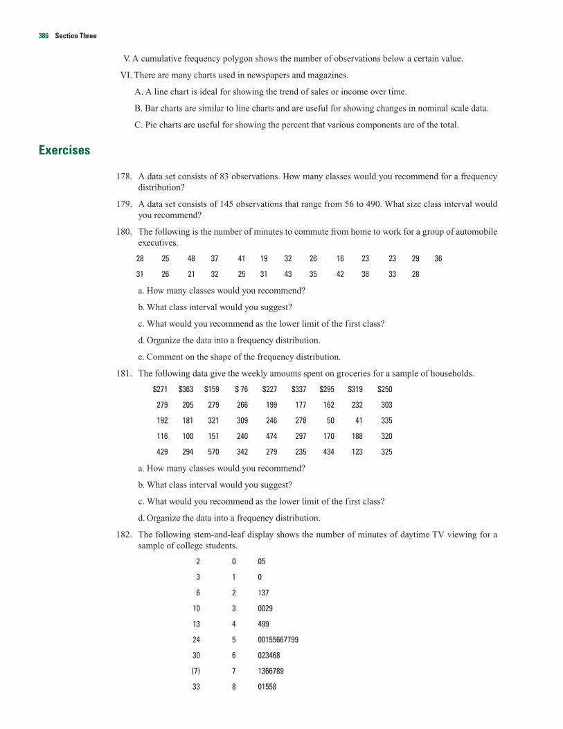
V. A cumulative frequency polygon shows the number of observations below a certain value.
VI. There are many charts used in newspapers and magazines.
A. A line chart is ideal for showing the trend of sales or income over time.
B. Bar charts are similar to line charts and are useful for showing changes in nominal scale data.
C. Pie charts are useful for showing the percent that various components are of the total.
Exercises
178. A data set consists of 83 observations. How many classes would you recommend for a frequencydistribution?
179. A data set consists of 145 observations that range from 56 to 490. What size class interval wouldyou recommend?
180. The following is the number of minutes to commute from home to work for a group of automobileexecutives.
28 25 48 37 41 19 32 26 16 23 23 29 36
31 26 21 32 25 31 43 35 42 38 33 28
a. How many classes would you recommend?
b. What class interval would you suggest?
c. What would you recommend as the lower limit of the first class?
d. Organize the data into a frequency distribution.
e. Comment on the shape of the frequency distribution.
181. The following data give the weekly amounts spent on groceries for a sample of households.
$271 $363 $159 $ 76 $227 $337 $295 $319 $250
279 205 279 266 199 177 162 232 303
192 181 321 309 246 278 50 41 335
116 100 151 240 474 297 170 188 320
429 294 570 342 279 235 434 123 325
a. How many classes would you recommend?
b. What class interval would you suggest?
c. What would you recommend as the lower limit of the first class?
d. Organize the data into a frequency distribution.
182. The following stem-and-leaf display shows the number of minutes of daytime TV viewing for asample of college students.
2 0 05
3 1 0
6 2 137
10 3 0029
13 4 499
24 5 00155667799
30 6 023468
(7) 7 1366789
33 8 01558
386 Section Three
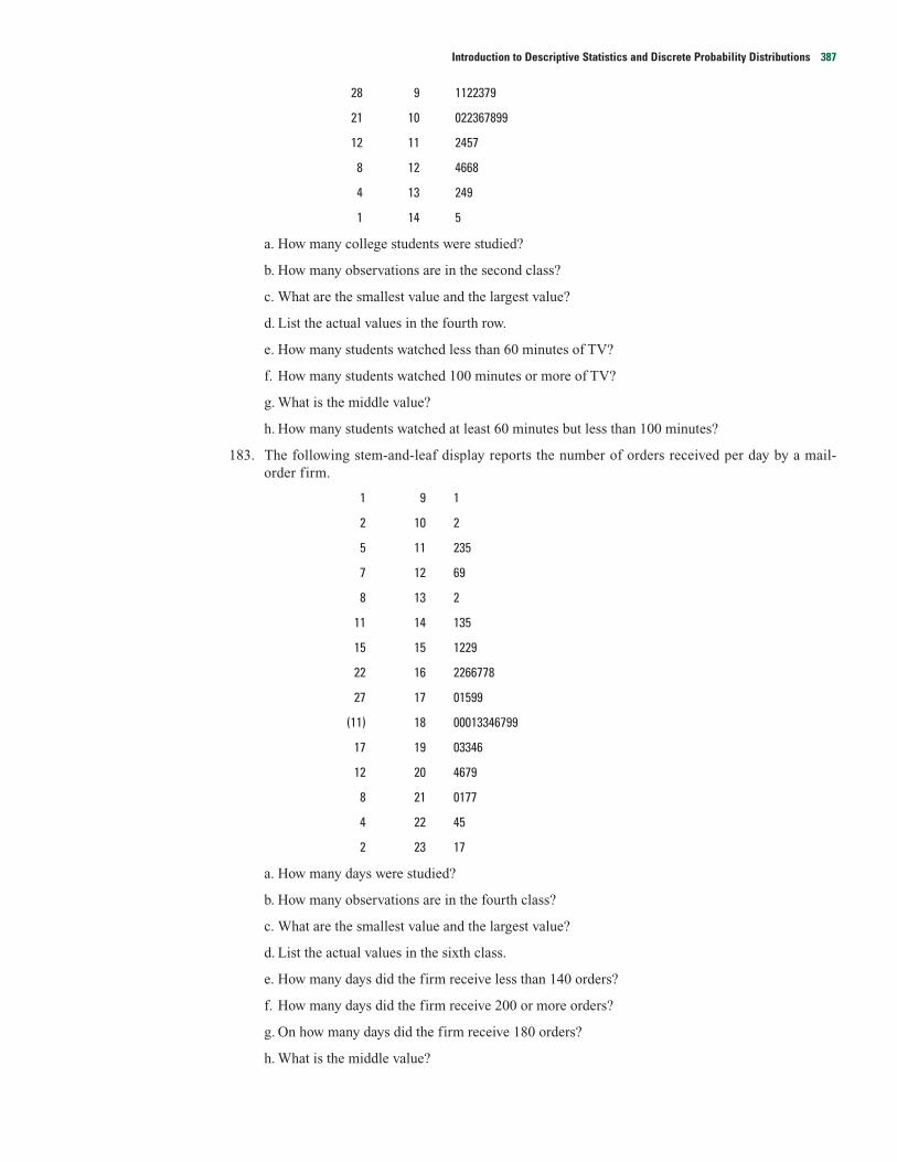
Introduction to Descriptive Statistics and Discrete Probability Distributions 387
28 9 1122379
21 10 022367899
12 11 2457
8 12 4668
4 13 249
1 14 5
a. How many college students were studied?
b. How many observations are in the second class?
c. What are the smallest value and the largest value?
d. List the actual values in the fourth row.
e. How many students watched less than 60 minutes of TV?
f. How many students watched 100 minutes or more of TV?
g. What is the middle value?
h. How many students watched at least 60 minutes but less than 100 minutes?
183. The following stem-and-leaf display reports the number of orders received per day by a mail-order firm.
1 9 1
2 10 2
5 11 235
7 12 69
8 13 2
11 14 135
15 15 1229
22 16 2266778
27 17 01599
(11) 18 00013346799
17 19 03346
12 20 4679
8 21 0177
4 22 45
2 23 17
a. How many days were studied?
b. How many observations are in the fourth class?
c. What are the smallest value and the largest value?
d. List the actual values in the sixth class.
e. How many days did the firm receive less than 140 orders?
f. How many days did the firm receive 200 or more orders?
g. On how many days did the firm receive 180 orders?
h. What is the middle value?

388 Section Three
184. The following histogram shows the scores on the first statistics exam.
a. How many students took the exam?
b. What is the class interval?
c. What is the class midpoint for the first class?
d. How many students earned a score of less than 70?
185. The following chart summarizes the selling price of homes sold last month in the Sarasota,Florida, area.
a. What is the chart called?
b. How many homes were sold during the last month?
c. What is the class interval?
d. About 75 percent of the houses sold for less than what amount?
e. One hundred seventy-five of the homes sold for less than what amount?
186. A chain of sport shops catering to beginning skiers, headquartered in Aspen, Colorado, plans toconduct a study of how much a beginning skier spends on his or her initial purchase of equipmentand supplies. Based on these figures, they want to explore the possibility of offering combinations,such as a pair of boots and a pair of skis, to induce customers to buy more. A sample of their cashregister receipts revealed these initial purchases:
$140 $ 82 $265 $168 $ 90 $114 $172 $230 $142
86 125 235 212 171 149 156 162 118
139 149 132 105 162 126 216 195 127
161 135 172 220 229 129 87 128 126
175 127 149 126 121 118 172 126
a. Arrive at a suggested class interval. Use five classes, and let the lower limit of the first classbe $80.
b. What would be a better class interval?
c. Organize the data into a frequency distribution using a lower limit of $80.
d. Interpret your findings.
100
75
50
25
250200150100 50
0 50 100 150Selling price ($000)
200 250 300 350
Freq
uenc
y
Perc
ent
50 60 70 80 90 100
2520151050
Score
Freq
uenc
y
3
14
21
12
6

187. The numbers of shareholders for a selected group of large companies (in thousands) are:
Number of Number ofShareholders Shareholders
Company (thousands) Company (thousands)
Pan American World Airways 144 Northeast Utilities 200
General Public Utilities 177 Standard Oil (Indiana) 173
Occidental Petroleum 266 Home Depot 195
Middle South Utilities 133 Detroit Edison 220
DaimlerChrysler 209 Eastman Kodak 251
Standard Oil of California 264 Dow Chemical 137
Bethlehem Steel 160 Pennsylvania Power 150
Long Island Lighting 143 American Electric Power 262
RCA 246 Ohio Edison 158
Greyhound Corporation 151 Transamerica Corporation 162
Pacific Gas & Electric 239 Columbia Gas System 165
Niagara Mohawk Power 204 International Telephone &
E. I. du Pont de Nemours 204 Telegraph 223
Westinghouse Electric 195 Union Electric 158
Union Carbide 176 Virginia Electric and Power 162
BankAmerica 175 Public Service Electric & Gas 225
Consumers Power 161
The numbers of shareholders are to be organized into a frequency distribution and severalgraphs drawn to portray the distribution.
a. Using seven classes and a lower limit of 130, construct a frequency distribution.
b. Portray the distribution as a frequency polygon.
c. Portray the distribution in a cumulative frequency polygon.
d. Based on the polygon, three out of four (75 percent) of the companies have how many share-holders or less?
e. Write a brief analysis of the number of shareholders based on the frequency distribution andgraphs.
188. A recent survey showed that the typical American car owner spends $2,950 per year on operatingexpenses. Below is a breakdown of the various expenditure items. Draw an appropriate chart toportray the data and summarize your findings in a brief report.
Expenditure Item Amount
Fuel $ 603
Interest on car loan 279
Repairs 930
Insurance and license 646
Depreciation 492
Total $2,950
Introduction to Descriptive Statistics and Discrete Probability Distributions 389

189. The Midland National Bank selected a sample of 40 student checking accounts. Below are theirend-of-the-month balances.
$404 $ 74 $234 $149 $279 $215 $123 $ 55 $ 43 $321
87 234 68 489 57 185 141 758 72 863
703 125 350 440 37 252 27 521 302 127
968 712 503 489 327 608 358 425 303 203
a. Tally the data into a frequency distribution using $100 as a class interval and $0 as the startingpoint.
b. Draw a cumulative frequency polygon.
c. The bank considers any student with an ending balance of $400 or more a “preferred customer.”Estimate the percentage of preferred customers.
d. The bank is also considering a service charge to the lowest 10 percent of the ending balances.What would you recommend as the cutoff point between those who have to pay a service chargeand those who do not?
190. The United States Department of Transportation keeps track of the percentage of flights that arrivewithin 15 minutes of the scheduled time, by airline. Below is the latest information. Construct astem-and-leaf chart from these data. Summarize your conclusion.
Airline Percent on Time Airline Percent on Time
Pan Am 82.7 American 78.1
America West 82.7 United 76.4
Northwest 81.0 Delta 76.1
USAir 80.1 Continental 76.9
Southwest 79.7 British Airways 80.4
Alaska 79.7 Japan Airlines 81.4
191. A recent study of home technologies reported the number of hours of personal computer usage perweek for a sample of 60 persons. Excluded from the study were people who worked out of theirhome and used the computer as a part of their work.
9.3 5.3 6.3 8.8 6.5 0.6 5.2 6.6 9.3 4.3
6.3 2.1 2.7 0.4 3.7 3.3 1.1 2.7 6.7 6.5
4.3 9.7 7.7 5.2 1.7 8.5 4.2 5.5 5.1 5.6
5.4 4.8 2.1 10.1 1.3 5.6 2.4 2.4 4.7 1.7
2.0 6.7 1.1 6.7 2.2 2.6 9.8 6.4 4.9 5.2
4.5 9.3 7.9 4.6 4.3 4.5 9.2 8.5 6.0 8.1
a. Organize the data into a frequency distribution. How many classes would you suggest? Whatvalue would you suggest for a class interval?
b. Draw a histogram. Interpret your result.
192. Merrill Lynch recently completed a study regarding the size of investment portfolios (stocks,bonds, mutual funds, and certificates of deposit) for a sample of clients in the 40 to 50 age group.Listed below is the value of all the investments for the 70 participants in the study.
669.9 7.5 77.2 7.5 125.7 516.9 219.9 645.2
301.9 235.4 716.4 145.3 26.6 187.2 315.5 89.2
136.4 616.9 440.6 408.2 34.4 296.1 185.4 526.3
390 Section Three
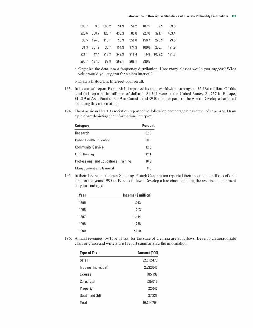
Introduction to Descriptive Statistics and Discrete Probability Distributions 391
380.7 3.3 363.2 51.9 52.2 107.5 82.9 63.0
228.6 308.7 126.7 430.3 82.0 227.0 321.1 403.4
39.5 124.3 118.1 23.9 352.8 156.7 276.3 23.5
31.3 301.2 35.7 154.9 174.3 100.6 236.7 171.9
221.1 43.4 212.3 243.3 315.4 5.9 1002.2 171.7
295.7 437.0 87.8 302.1 268.1 899.5
a. Organize the data into a frequency distribution. How many classes would you suggest? Whatvalue would you suggest for a class interval?
b. Draw a histogram. Interpret your result.
193. In its annual report ExxonMobil reported its total worldwide earnings as $5,886 million. Of thistotal (all reported in millions of dollars), $1,541 were in the United States, $1,757 in Europe,$1,219 in Asia-Pacific, $439 in Canada, and $930 in other parts of the world. Develop a bar chartdepicting this information.
194. The American Heart Association reported the following percentage breakdown of expenses. Drawa pie chart depicting the information. Interpret.
Category Percent
Research 32.3
Public Health Education 23.5
Community Service 12.6
Fund Raising 12.1
Professional and Educational Training 10.9
Management and General 8.6
195. In their 1999 annual report Schering-Plough Corporation reported their income, in millions of dol-lars, for the years 1995 to 1999 as follows. Develop a line chart depicting the results and commenton your findings.
Year Income ($ million)
1995 1,053
1996 1,213
1997 1,444
1998 1,756
1999 2,110
196. Annual revenues, by type of tax, for the state of Georgia are as follows. Develop an appropriatechart or graph and write a brief report summarizing the information.
Type of Tax Amount (000)
Sales $2,812,473
Income (Individual) 2,732,045
License 185,198
Corporate 525,015
Property 22,647
Death and Gift 37,326
Total $6,314,704

197. Annual imports from selected Canadian trading partners are listed below. Develop an appropriatechart or graph and write a brief report summarizing the information.
Partner Annual Imports (million)
Japan $9,550
United Kingdom 4,556
South Korea 2,441
China 1,182
Australia 618
198. Farming has changed from the early 1900s. In the early 20th century, machinery gradually replacedanimal power. For example, in 1910 U.S. farms used 24.2 million horses and mules and only about1,000 tractors. By 1960, 4.6 million tractors were used and only 3.2 million horses and mules. In1920 there were over 6 million farms in the United States. Today there are less than 2 million.Listed below is the number of farms, in thousands, for each of the 50 states. Write a paragraphsummarizing your findings.
47 1 8 46 76 26 4 3 39 45
4 21 80 63 100 65 91 29 7 15
7 52 87 39 106 25 55 2 3 8
14 38 59 33 76 71 37 51 1 24
35 86 185 13 7 43 36 20 79 9
199. One of the most popular candies in the United States is M&M’s, which is produced by the MarsCompany. For many years the M&M’s plain candies were produced in six colors: red, green,orange, tan, brown, and yellow. Recently, tan was replaced by blue. Did you ever wonder how manycandies were in a bag, or how many of each color? Are there about the same number of each color,or are there more of some colors than others? Here is some information for a one-pound bag ofM&M’s plain candies. It contained a total of 544 candies. There were 135 brown, 156 yellow, 128red, 22 green, 50 blue, and 53 orange. Develop a chart depicting this information and a brief reportsummarizing the information.
200. The following graph compares the average selling prices of the Ford Taurus and the Toyota Camryfrom 1993 to 2000. Write a brief report summarizing the information in the graph. Be sure toinclude the selling price of the two cars, the change in the selling price, and the direction of thechange in the eight-year period.
exercises.com
201. Monthly and year-to-date truck sales are available at the website: http://www.pickuptruck.com.Go to this site and under Features click on News to obtain the most recent information. Make apie chart or a bar chart showing the most recent information. What is the best selling truck? Whatare the four or five best selling trucks? What is their market share? You may wish to group some
22.0
18.0
14.0
10.0
93 94 95 96 97 98 99 00Year
Camry
Taurus
Pric
e($
000)
392 Section Three

of the trucks into a category called “Other” to get a better picture of market share. Comment onyour findings.
202. Go to an employment website such as http://jobsearch.monster.com. Click on Jobs and select a geo-graphic region and an area of specialization of interest to you. For example, you might select theOrlando, Florida region and Banking as your area of interest. Make a stem-and-leaf display of thesalaries offered for the various jobs. To make valid comparisons convert all wages to a yearly basis(assume 40 hours per week and 50 weeks in a year). Where a range is given for salaries, use the cen-ter of the range. Then write a brief summary describing the typical salary and the shape of the dis-tribution.
Computer Data Exercises
203. Refer to the Real Estate data, which reports information on homes sold in the Venice, Florida areaduring the last year (Appendix J).
a. Select an appropriate class interval and organize the selling prices into a frequencydistribution.
1. Around what values do the data tend to cluster?
2. What is the largest selling price? What is the smallest selling price?
b. Draw a cumulative frequency distribution based on the frequency distributiondeveloped in Part a.
1. How many homes sold for less than $200,000?
2. Estimate the percent of the homes that sold for more than $220,000.
3. What percent of the homes sold for less than $125,000?
c. Write a report summarizing the selling prices of the homes.
204. Refer to the Baseball 2000 data, which reports information on the 30 Major League Baseball teamsfor the 2000 season (Appendix K).
a. Organize the information on the team salaries into a frequency distribution. Select anappropriate class interval.
1. What is a typical team salary? What is the range of salaries?
2. Comment on the shape of the distribution. Does it appear that any of the team salaries are outof line with the others?
b. Draw a cumulative frequency distribution based on the frequency distributiondeveloped in Part a.
1. Forty percent of the teams are paying less than what amount in total team salary?
2. About how many teams have total salaries of less than $50,000,000?
3.Below what amount do the lowest five teams pay in total salary?
c. Organize the information on the size of the various stadiums into a frequencydistribution.
1. What is a typical stadium size? Where do the stadium sizes tend to cluster?
2. Comment on the shape of the distribution. Does it appear that any of the stadium sizes are outof line with the others?
Introduction to Descriptive Statistics and Discrete Probability Distributions 393
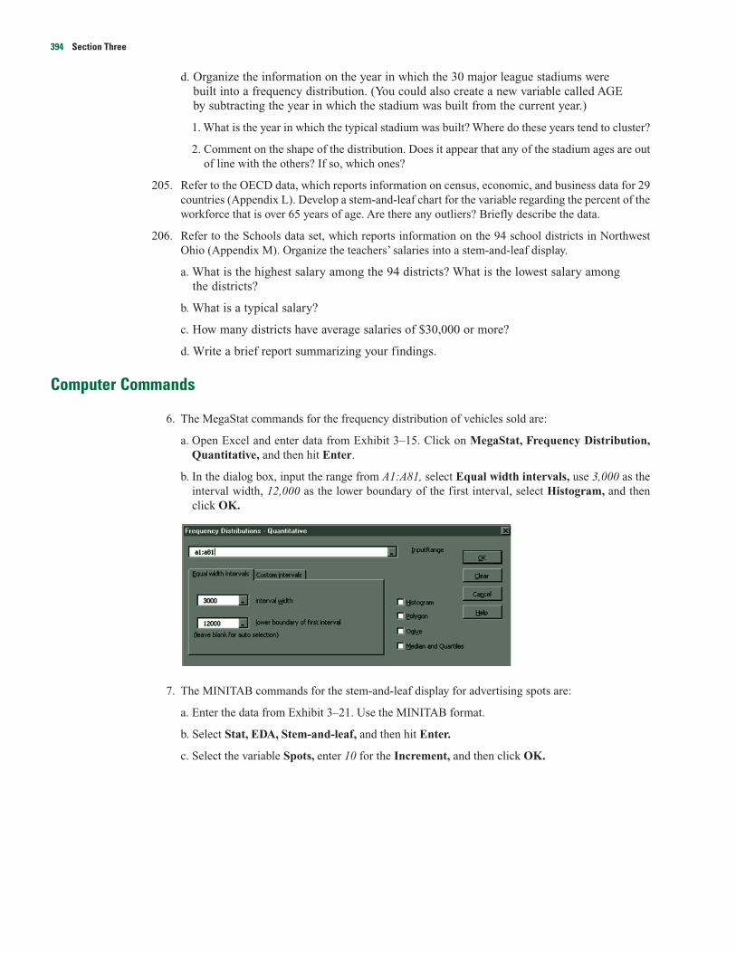
d. Organize the information on the year in which the 30 major league stadiums werebuilt into a frequency distribution. (You could also create a new variable called AGEby subtracting the year in which the stadium was built from the current year.)
1. What is the year in which the typical stadium was built? Where do these years tend to cluster?
2. Comment on the shape of the distribution. Does it appear that any of the stadium ages are outof line with the others? If so, which ones?
205. Refer to the OECD data, which reports information on census, economic, and business data for 29countries (Appendix L). Develop a stem-and-leaf chart for the variable regarding the percent of theworkforce that is over 65 years of age. Are there any outliers? Briefly describe the data.
206. Refer to the Schools data set, which reports information on the 94 school districts in NorthwestOhio (Appendix M). Organize the teachers’ salaries into a stem-and-leaf display.
a. What is the highest salary among the 94 districts? What is the lowest salary amongthe districts?
b. What is a typical salary?
c. How many districts have average salaries of $30,000 or more?
d. Write a brief report summarizing your findings.
Computer Commands
6. The MegaStat commands for the frequency distribution of vehicles sold are:
a. Open Excel and enter data from Exhibit 3–15. Click on MegaStat, Frequency Distribution,Quantitative, and then hit Enter.
b. In the dialog box, input the range from A1:A81, select Equal width intervals, use 3,000 as theinterval width, 12,000 as the lower boundary of the first interval, select Histogram, and thenclick OK.
7. The MINITAB commands for the stem-and-leaf display for advertising spots are:
a. Enter the data from Exhibit 3–21. Use the MINITAB format.
b. Select Stat, EDA, Stem-and-leaf, and then hit Enter.
c. Select the variable Spots, enter 10 for the Increment, and then click OK.
394 Section Three
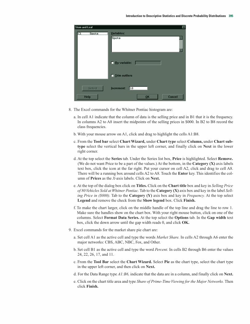
8. The Excel commands for the Whitner Pontiac histogram are:
a. In cell A1 indicate that the column of data is the selling price and in B1 that it is the frequency.In columns A2 to A8 insert the midpoints of the selling prices in $000. In B2 to B8 record theclass frequencies.
b. With your mouse arrow on A1, click and drag to highlight the cells A1:B8.
c. From the Tool bar select Chart Wizard, under Chart type select Column, under Chart sub-type select the vertical bars in the upper left corner, and finally click on Next in the lowerright corner.
d. At the top select the Series tab. Under the Series list box, Price is highlighted. Select Remove.(We do not want Price to be a part of the values.) At the bottom, in the Category (X) axis labelstext box, click the icon at the far right. Put your cursor on cell A2, click and drag to cell A8.There will be a running box around cells A2 to A8. Touch the Enter key. This identifies the col-umn of Prices as the X-axis labels. Click on Next.
e. At the top of the dialog box click on Titles. Click on the Chart title box and key in Selling Priceof 80 Vehicles Sold at Whitner Pontiac. Tab to the Category (X) axis box and key in the label Sell-ing Price in ($000). Tab to the Category (Y) axis box and key in Frequency. At the top selectLegend and remove the check from the Show legend box. Click Finish.
f. To make the chart larger, click on the middle handle of the top line and drag the line to row 1.Make sure the handles show on the chart box. With your right mouse button, click on one of thecolumns. Select Format Data Series. At the top select the Options tab. In the Gap width textbox, click the down arrow until the gap width reads 0, and click OK.
9. Excel commands for the market share pie chart are:
a. Set cell A1 as the active cell and type the words Market Share. In cells A2 through A6 enter themajor networks: CBS, ABC, NBC, Fox, and Other.
b. Set cell B1 as the active cell and type the word Percent. In cells B2 through B6 enter the values24, 22, 26, 17, and 11.
c. From the Tool Bar select the Chart Wizard. Select Pie as the chart type, select the chart typein the upper left corner, and then click on Next.
d. For the Data Range type A1:B6, indicate that the data are in a column, and finally click on Next.
e. Click on the chart title area and type Share of Prime-Time Viewing for the Major Networks. Thenclick Finish.
Introduction to Descriptive Statistics and Discrete Probability Distributions 395

396 Section Three
Answers to Self-Review3–17 a. The raw data.
b.Number of
Commission Salespeople
$1,400 up to $1,500 21,500 up to 1,600 51,600 up to 1,700 31,700 up to 1,800 1
Total 11
c. Class frequencies.d. The largest concentration of commissions is $1,500
up to $1,600. The smallest commission is about$1,400 and the largest is about $1,800.
3–18 a. 26 � 64 � 70 � 128 � 27. So 7 classes arerecommended.
b. The interval width should be at least (550 � 340)/7 �30. So 35 feet would be a reasonable interval width.
c. Classes: 325 up to 360 feet, 360 up to 395 feet, 395up to 430 feet, 430 up to 465 feet, 465 up to 500 feet,500 up to 535 feet, and 535 up to 570 feet.
3–19 a. 23b. 28.75%, found by (23/80) � 100c. 7.5%, found by (6/80) � 100.
3–207 78 00134889 1256689
10 124811 26
a. 8b. 10.1, 10.2, 10.4, 10.8c. 9.5d. 7.7, 11.6
3–21 a.
b.
c. The smallest annual sales volume of imports by asupplier is about $2 million, the highest about $17million. The concentration is between $8 million and$11 million.
3–22 a. A frequency distribution.b.
Hourly Wages Cumulative Number
Less than $6 0Less than $8 3Less than $10 10Less than $12 14Less than $14 15
c. About 7 employees earn $9.00 or less. About half theemployees earn $9.25 or more. About 4 employeesearn $8.25 or less.
3–23
4% Supplies
90%95% 0% 5%
10%
15%
20%
25%
30%
35%
40%45%50%55%
60%
85%
80%
75%
70%
65%
16% Administration
58%Roads
22%Schools
6 8 10 12 14
Cum
ulat
ive
frequ
enci
es
Hourly wages (in dollars)
X = 10Y = 10
15
12
8
4
0
X = 12Y = 14
40
30
20
10
02 5 8 11 14 17
Imports ($ millions)
Perc
ent o
f tot
al
20
15
10
5
02 5 8 11 14 17
Imports ($ millions)
Num
ber o
fsu
pplie
rs
6
13
20
10
1

Discrete Probability
Introduction: What is a Probability?Earlier we organized the prices of 80 vehicles sold last month at Whitner Pontiac into a frequencydistribution. This frequency distribution shows the lowest and the highest selling prices and wherethe largest concentration of data occur. We also used a number of measures of central tendency anddispersion to locate a typical selling price (about $20,000) and to examine the spread in the data.We describe the spread in the selling prices with such measures of dispersion as the range and thestandard deviation. Descriptive statistics is concerned with summarizing that which has alreadyhappened. For example, we described the vehicle selling prices last month at Whitner Pontiac.
We now turn to the second facet of statistics, namely, computing the chance that something willoccur in the future. This facet of statistics is called statistical inference or inferential statistics.
Seldom does a decision maker have complete information from which to make a decision. Forexample:
• Toys and Things, a toy and puzzle manufacturer, recently developed a new game based on sportstrivia. They want to know whether sports buffs will purchase the game. “Slam Dunk” and “HomeRun” are two of the names under consideration. One way to minimize the risk of making a wrongdecision is to hire pollsters to take a sample of, say, 2,000 from the population and ask each respon-dent for a reaction to the new game and its proposed titles.
• The quality assurance department of a Bethlehem Steel mill must assure management that the quar-ter-inch wire being produced has an acceptable tensile strength. Obviously, not all the wire pro-duced can be tested for tensile strength because testing requires the wire to be stretched until itbreaks—thus destroying it. So a random sample of 10 pieces is selected and tested. Based on thetest results, all the wire produced is deemed to be either satisfactory or unsatisfactory.
• Other questions involving uncertainty are: Should the daytime drama Days of Our Lives be dis-continued immediately? Should the New York Giants select Sammy Uwea or Clint Murray in thefirst round of the college draft? Will a newly developed mint-flavoredcereal be profitable if mar-keted? Should I marry Jean? Should I buy a new Rolls Royce? Should I vote for Charles Lindenfor town commissioner?
Statistical inference deals with conclusions about a population based on a sample taken fromthat population. (The populations for the preceding illustrations are: all consumers who likesports trivia games, all the quarter-inch steel wire produced, all television viewers who watchsoaps, all the college football players to be drafted by the professional teams, and so on.)
Because there is uncertainty in decision making, it is important that all the known risksinvolved be scientifically evaluated. Helpful in this evaluation is probability theory, which hasoften been referred to as the science of uncertainty. The use of probability theory allows the deci-sion maker with only limited information to analyze the risks and minimize the gamble inherent,for example, in marketing a new product or accepting an incoming shipment possibly containingdefective parts.
Because probability concepts are so important in the field of statistical inference, this sectionintroduces the basic language of probability, including such terms as experiment, event, subjec-tive probability, and addition and multiplication rules.
No doubt you are familiar with terms such as probability, chance, and likelihood. They areoften used interchangeably. The weather forecaster announces that there is a 70 percent chance ofrain for Super Bowl Sunday. Based on a survey of consumers who tested a newly developedpickle with a banana taste, the probability is .03 that, if marketed, it will be a financial success.(This means that the chance of the banana-tasting pickle being accepted by the public is ratherremote.) What is a probability? In general, it is a number that describes the chance that somethingwill happen.
Introduction to Descriptive Statistics and Discrete Probability Distributions 397
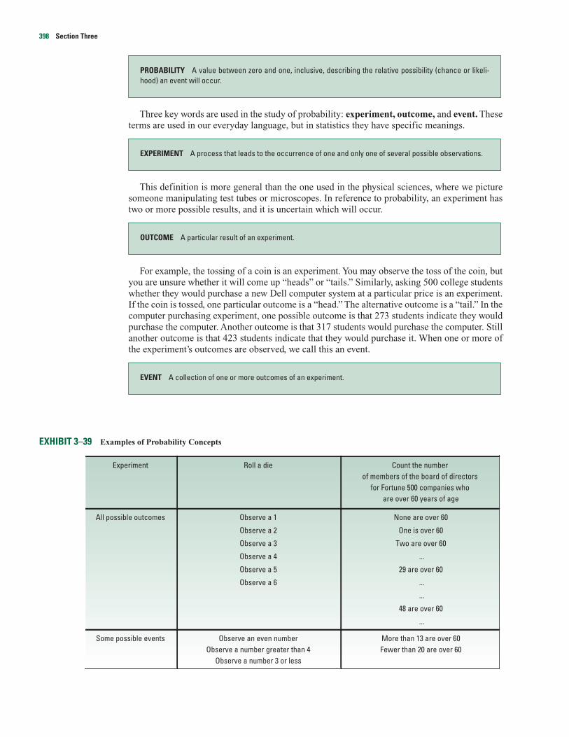
Three key words are used in the study of probability: experiment, outcome, and event. Theseterms are used in our everyday language, but in statistics they have specific meanings.
This definition is more general than the one used in the physical sciences, where we picturesomeone manipulating test tubes or microscopes. In reference to probability, an experiment hastwo or more possible results, and it is uncertain which will occur.
For example, the tossing of a coin is an experiment. You may observe the toss of the coin, butyou are unsure whether it will come up “heads” or “tails.” Similarly, asking 500 college studentswhether they would purchase a new Dell computer system at a particular price is an experiment.If the coin is tossed, one particular outcome is a “head.” The alternative outcome is a “tail.” In thecomputer purchasing experiment, one possible outcome is that 273 students indicate they wouldpurchase the computer. Another outcome is that 317 students would purchase the computer. Stillanother outcome is that 423 students indicate that they would purchase it. When one or more ofthe experiment’s outcomes are observed, we call this an event.
EXHIBIT 3–39 Examples of Probability Concepts
Experiment
All possible outcomes
Some possible events
Roll a die
Observe a 1
Observe a 2
Observe a 3
Observe a 4
Observe a 5
Observe a 6
Observe an even numberObserve a number greater than 4
Observe a number 3 or less
Count the number of members of the board of directors
for Fortune 500 companies who are over 60 years of age
None are over 60
One is over 60
Two are over 60
...
29 are over 60
...
...
48 are over 60
...
More than 13 are over 60Fewer than 20 are over 60
EVENT A collection of one or more outcomes of an experiment.
OUTCOME A particular result of an experiment.
EXPERIMENT A process that leads to the occurrence of one and only one of several possible observations.
PROBABILITY A value between zero and one, inclusive, describing the relative possibility (chance or likeli-hood) an event will occur.
398 Section Three

Examples to clarify the definitions of the terms experiment, outcome, and event are given inExhibit 3–39.
In the die-rolling experiment there are six possible outcomes, but there are many possibleevents. When counting the number of members of the board of directors for Fortune 500 compa-nies over 60 years of age, the number of possible outcomes can be anywhere from zero to thetotal number of members. There are an even larger number of possible events in this experiment.
A probability is frequently expressed as a decimal, such as .70, .27, or .50. However, it may begiven as a fraction such as 7/10, 27/100, or 1/2. It can assume any number from 0 to 1, inclusive.If a company has only five sales regions, and each region’s name or number is written on a slipof paper and the slips put in a hat, the probability of selecting one of the five regions is 1. Theprobability of selecting from the hat a slip of paper that reads “Pittsburgh Steelers” is 0. Thus, theprobability of 1 represents something that is certain to happen, and the probability of 0 repre-sents something that cannot happen.
The closer a probability is to 0, the more improbable it is the event will happen. The closer theprobability is to 1, the more sure we are it will happen. The relationship is shown in Exhibit 3–40along with a few of our personal beliefs. You might, however, select a different probability for SloPoke’s chances to win the Kentucky Derby or for an increase in federal taxes.
EXHIBIT 3–40 Ranges of Probability
Self-Review 3–24
Approaches to ProbabilityTwo approaches to probability will be discussed, namely, the objective and the subjective view-points. Objective probability is subdivided into (1) classical probability and (2) empiricalprobability.
Video Games, Inc. recently developed a new video game. Its market potential is to be tested by 80 vet-eran game players.
(a) What is the experiment?
(b) What is one possible outcome?
(c) Suppose 65 players tried the new game and said they liked it. Is 65 a probability?
(d) The probability that the new game will be a success is computed to be �1. Comment.
(e) Specify one possible event.
Cannot Sure tohappen happen
0.00 0.10 0.20 0.30 0.40 0.50 0.60 0.70 0.80 0.90 1.00
Probabilityour sun willdisappear this year
Chance SloPoke willwin the
KentuckyDerby
Chance of ahead in
single tossof a coin
Chanceof an
increasein federal
taxes
Chance of rain inFlorida
this year
Introduction to Descriptive Statistics and Discrete Probability Distributions 399
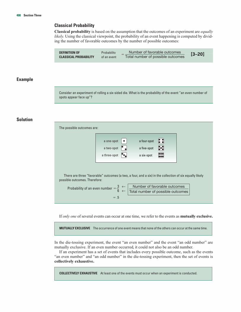
Classical ProbabilityClassical probability is based on the assumption that the outcomes of an experiment are equallylikely. Using the classical viewpoint, the probability of an event happening is computed by divid-ing the number of favorable outcomes by the number of possible outcomes:
DEFINITION OF ProbabilityCLASSICAL PROBABILITY of an event
[3–20]
Example
Solution
The possible outcomes are:
There are three “favorable” outcomes (a two, a four, and a six) in the collection of six equally likelypossible outcomes. Therefore:
Probability of an even number �3 ←6 ←
� .5
If only one of several events can occur at one time, we refer to the events as mutually exclusive.
In the die-tossing experiment, the event “an even number” and the event “an odd number” aremutually exclusive. If an even number occurred, it could not also be an odd number.
If an experiment has a set of events that includes every possible outcome, such as the events“an even number” and “an odd number” in the die-tossing experiment, then the set of events iscollectively exhaustive.
COLLECTIVELY EXHAUSTIVE At least one of the events must occur when an experiment is conducted.
MUTUALLY EXCLUSIVE The occurrence of one event means that none of the others can occur at the same time.
Number of favorable outcomesTotal number of possible outcomes
a one-spot
a two-spot
a three-spot
a four-spot
a five-spot
a six-spot
Consider an experiment of rolling a six-sided die. What is the probability of the event “an even number ofspots appear face up”?
�Number of favorable outcomes
Total number of possible outcomes
400 Section Three

For the die-tossing experiment, every outcome will be either even or odd. So the set is collectivelyexhaustive.
If the set of events is collectively exhaustive and the events are mutually exclusive, the sum ofthe probabilities equals 1. For a coin-tossing experiment:
Probability
Event: Head .5
Event: Tail .5
Total 1.0
For the classical approach to be applied, the events must have the same chance of occurring(called equally likely events). Also, the set of events must be mutually exclusive and collectivelyexhaustive.
Historically, the classical approach to probability was developed and applied in the 17th and18th centuries to games of chance, such as cards and dice. Note that it is unnecessary to do anexperiment to determine the probability of an event occurring using the classical approach; wecan logically arrive, for example, at the probability of getting a tail on the toss of one coin orthree heads on the toss of three coins. Nor do we have to conduct an experiment to determine theprobability that your income tax return will be audited if there are 2 million returns mailed toyour district office and 2,400 are to be audited. Assuming that each return has an equal chance ofbeing audited, your probability is .0012—found by 2,400 divided by 2 million. Obviously, thechance of your return being audited is rather remote.
Empirical ConceptAnother way to define probability is based on relative frequencies. The probability of an eventhappening is determined by observing what fraction of the time similar events happened in thepast. In terms of a formula:
Probability of event happening �
Example
Solution
Probability of event happening �
P(A) �
� .51
To simplify, letters or numbers may be used. P stands for probability, and in this case P(A) stands forthe probability a graduate is not employed in his or her major area of college study.
Since 383 out of 751, or .51 in terms of a probability, are in a different field of employment from theirmajor in college, we can use this as an estimate of the probability. In other words, based on past experi-ence, the probability is .51 that a new business graduate will be employed in a field other than his or hercollege major.
383751
Number of times event occurred in pastTotal number of observations
A study of 751 business administration graduates of the University of Toledo revealed 383 of the 751 werenot employed in their major area of study in college. For illustration, a person who majored in accountingis now the marketing manager of a tomato-processing firm. What is the probability that a particular busi-ness graduate will be employed in an area other than his or her college major?
Number of times event occurred in pastTotal number of observations
Introduction to Descriptive Statistics and Discrete Probability Distributions 401
Subjective ProbabilityIf there is little or no past experience on which to base a probability, it may be arrived at subjec-tively. Essentially, this means evaluating the available opinions and other information and thenestimating or assigning the probability. This probability is aptly called a subjective probability.
Illustrations of subjective probability are:
1. Estimating the likelihood the New England Patriots will play in the Super Bowl next year.
2. Estimating the probability General Motors Corp. will lose its number 1 ranking in total units soldto Ford Motor Co. or DaimlerChrysler within two years.
3. Estimating the likelihood you will earn an A in this course.
In summary, there are two viewpoints regarding probability—the objective and the subjectiveviewpoints. We noted that a probability statement always constitutes an estimate of an unknownvalue that will govern an event that has not yet occurred. There is, of course, a considerable lati-tude in the degree of uncertainty that surrounds this estimate, based primarily on the knowledgepossessed by the individual concerning the underlying process. The individual possesses a greatdeal of knowledge about the toss of a die and can state that the probability that a one-spot willappear face up on the toss of a true die is one-sixth. But we know very little concerning the accep-tance in the marketplace of a new and untested product. For example, even though a marketresearch director tests a newly developed product in 40 retail stores and states that there is a 70percent chance that the product will have sales of more than 1 million units, she still has littleknowledge of how consumers will react when it is marketed nationally. In both cases (the case ofthe person rolling a die and the testing of a new product) the individual is assigning a probabilityvalue to an event of interest, and a difference exists only in the predictor’s confidence in the pre-cision of the estimate. However, regardless of the viewpoint, the same laws of probability (pre-sented in the following sections) will be applied.
Self-Review 3–25
Exercises
207. Some people are in favor of reducing Social Security benefits in order to achieve a balanced bud-get and others are against it. Two persons are selected and their opinions are recorded. List the pos-sible outcomes.
1. One card will be randomly selected from a standard 52-card deck. What is the probability the cardwill be a queen? Which approach to probability did you use to answer this question?
2. The National Center for Health Statistics reports that of 883 deaths, 24 resulted from an automobileaccident, 182 from cancer, and 333 from heart disease. What is the probability that a particular deathis due to an automobile accident? Which approach to probability did you use to answer this question?
3. What is the probability that the Dow Jones Industrial Average will exceed 12,000? Which approach toprobability did you use to answer this question?
SUBJECTIVE CONCEPT OF PROBABILITY The likelihood (probability) of a particular event happening that isassigned by an individual based on whatever information is available.
402 Section Three
208. A quality control inspector selects a part to be tested. The part is then declared acceptable,repairable, or scrapped. Then another part is tested. List the possible outcomes of this experimentregarding two parts.
209. A survey of 34 students at the Wall College of Business showed the following majors:
Accounting 10
Finance 5
Info. Systems 3
Management 6
Marketing 10
Suppose you select a student and observe his or her major.
a. What is the probability he or she is a management major?
b. Which concept of probability did you use to make this estimate?
210. A large company that must hire a new president prepares a final list of five candidates, all of whomare equally qualified. Two of these candidates are members of a minority group. The companydecides to select the president by lottery.
a. What is the probability one of the minority is hired?
b. Which concept of probability did you use to make this estimate?
211. The Streets Department in Whitehouse, Illinois, is considering widening Indiana Avenue to threelanes. Before a final decision is made, 500 citizens are asked if they support the widening.
a. What is the experiment?
b. What are some of the possible events?
c. List two possible outcomes.
212. The chairman of the board of Rudd Industries is delivering a speech to the company stockholderstomorrow explaining his position that the company should merge with Zimmerman Plastics. Hehas received six pieces of mail on the issue and is interested in the number of writers who agreewith him.
a. What is the experiment?
b. What are some of the possible events?
c. List two possible outcomes.
213. In each of the following cases, indicate whether classical, empirical, or subjective probability isused.
a. A basketball player makes 30 out of 50 foul shots. The probability is .6 that she makes the nextfoul shot attempted.
b. A seven-member committee of students is formed to study environmental issues. What is thelikelihood that any one of the seven is chosen as the spokesperson?
c. You purchase one of 5 million tickets sold for Lotto Canada. What is the likelihood you win the$1 million jackpot?
d. The probability of an earthquake in northern California in the next 10 years is .80.
214. A firm will promote two employees out of a group of six men and three women.
a. List the outcomes of this experiment if there is particular concern about gender equity.
b. Which concept of probability would you use to estimate these probabilities?
Introduction to Descriptive Statistics and Discrete Probability Distributions 403

215. There are 52 cards in a standard deck.
a. What is the probability that the first card selected is a spade?
b. What is the probability that the first card selected is the jack of spades?
c. What concept of probability do a. and b. illustrate?
216. A single die is rolled.
a. What is the probability that a two-spot will show face up?
b. What concept of probability does this illustrate?
c. Are the outcomes for the numbers 1 through 6 equally likely and mutually exclusive? Explain.
217. A sample of forty minority executives were selected to test a questionnaire. One question aboutenvironmental issues required a yes or no answer.
a. What is the experiment?
b. List one possible event.
c. Ten of the 40 executives responded “yes.” Based on these sample responses, what is the proba-bility an executive responded “yes”?
d. What concept of probability does this illustrate?
e. Are each of the possible outcomes equally likely and mutually exclusive?
218. A sample of 2000 licensed drivers revealed the following number of violations.
Number of Violations Number of Drivers
0 1,910
1 46
2 18
3 12
4 9
5 or more 5
Total 2,000
a. What is the experiment?
b. List one possible event.
c. What is the probability that a particular driver had exactly two violations?
d. What concept of probability does this illustrate?
219. Bank of America customers select their own three-digit personal identification number (PIN) foruse at ATMs.
a. Think of this as an experiment and list four possible outcomes.
b. What is the probability Mr. Jones and Mrs. Smith select the same PIN?
c. Which concept of probability did you use to answer the question above?
220. An investor buys 100 shares of AT&T stock and records its price change daily.
a. List several possible events for this experiment.
b. Estimate the probability for each event you described in a.
c. Which concept of probability did you use in b.?
404 Section Three
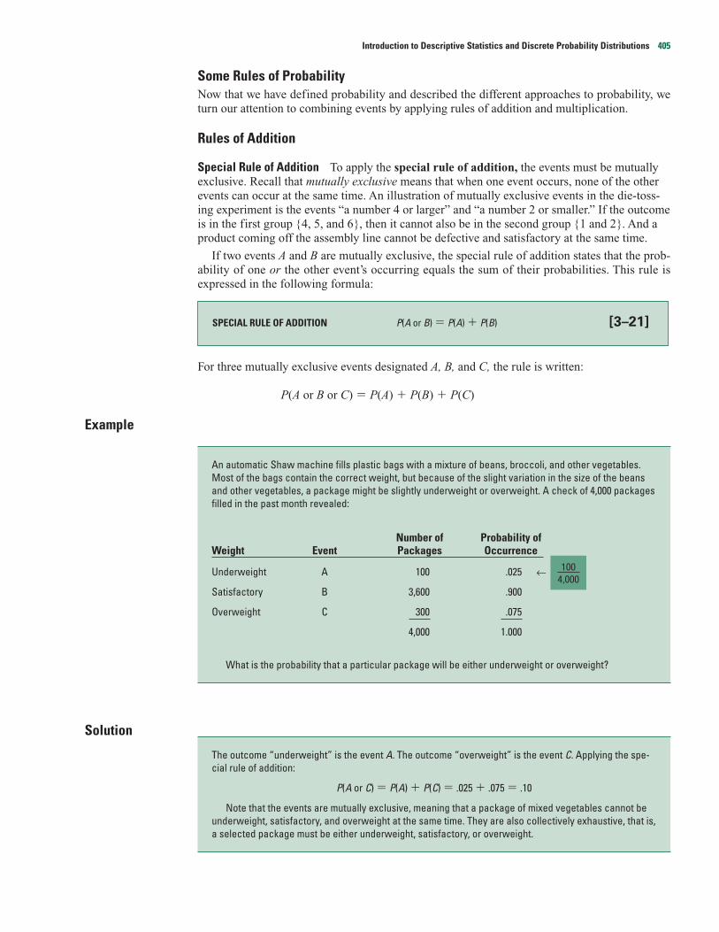
Some Rules of ProbabilityNow that we have defined probability and described the different approaches to probability, weturn our attention to combining events by applying rules of addition and multiplication.
Rules of Addition
Special Rule of Addition To apply the special rule of addition, the events must be mutuallyexclusive. Recall that mutually exclusive means that when one event occurs, none of the otherevents can occur at the same time. An illustration of mutually exclusive events in the die-toss-ing experiment is the events “a number 4 or larger” and “a number 2 or smaller.” If the outcomeis in the first group {4, 5, and 6}, then it cannot also be in the second group {1 and 2}. And aproduct coming off the assembly line cannot be defective and satisfactory at the same time.
If two events A and B are mutually exclusive, the special rule of addition states that the prob-ability of one or the other event’s occurring equals the sum of their probabilities. This rule isexpressed in the following formula:
For three mutually exclusive events designated A, B, and C, the rule is written:
P(A or B or C) � P(A) � P(B) � P(C)
Example
Solution
The outcome “underweight” is the event A. The outcome “overweight” is the event C. Applying the spe-cial rule of addition:
P(A or C) � P(A) � P(C) � .025 � .075 � .10
Note that the events are mutually exclusive, meaning that a package of mixed vegetables cannot beunderweight, satisfactory, and overweight at the same time. They are also collectively exhaustive, that is,a selected package must be either underweight, satisfactory, or overweight.
An automatic Shaw machine fills plastic bags with a mixture of beans, broccoli, and other vegetables.Most of the bags contain the correct weight, but because of the slight variation in the size of the beansand other vegetables, a package might be slightly underweight or overweight. A check of 4,000 packagesfilled in the past month revealed:
Number of Probability ofWeight Event Packages Occurrence
Underweight A 100 .025 ←
Satisfactory B 3,600 .900
Overweight C 300 .075
4,000 1.000
What is the probability that a particular package will be either underweight or overweight?
SPECIAL RULE OF ADDITION P(A or B) � P(A) � P(B) [3–21]
Introduction to Descriptive Statistics and Discrete Probability Distributions 405
1004,000
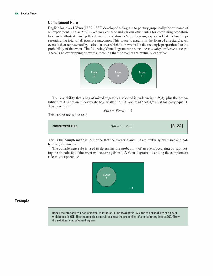
Complement RuleEnglish logician J. Venn (1835–1888) developed a diagram to portray graphically the outcome ofan experiment. The mutually exclusive concept and various other rules for combining probabili-ties can be illustrated using this device. To construct a Venn diagram, a space is first enclosed rep-resenting the total of all possible outcomes. This space is usually in the form of a rectangle. Anevent is then represented by a circular area which is drawn inside the rectangle proportional to theprobability of the event. The following Venn diagram represents the mutually exclusive concept.There is no overlapping of events, meaning that the events are mutually exclusive.
The probability that a bag of mixed vegetables selected is underweight, P(A), plus the proba-bility that it is not an underweight bag, written P(�A) and read “not A,” must logically equal 1.This is written:
P(A) � P(�A) � 1This can be revised to read:
This is the complement rule. Notice that the events A and �A are mutually exclusive and col-lectively exhaustive.
The complement rule is used to determine the probability of an event occurring by subtract-ing the probability of the event not occurring from 1. A Venn diagram illustrating the complementrule might appear as:
Example
Recall the probability a bag of mixed vegetables is underweight is .025 and the probability of an over-weight bag is .075. Use the complement rule to show the probability of a satisfactory bag is .900. Showthe solution using a Venn diagram.
EventA
�A
COMPLEMENT RULE P(A) � 1 � P(��) [3–22]
EventA
EventB
EventC
406 Section Three
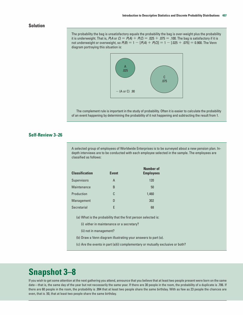
Solution
The probability the bag is unsatisfactory equals the probability the bag is over-weight plus the probabilityit is underweight. That is, P(A or C) � P(A) � P(C) � .025 � .075 � .100. The bag is satisfactory if it isnot underweight or overweight, so P(B) � 1 � [P(A) � P(C)] � 1 � [.025 � .075] � 0.900. The Venndiagram portraying this situation is:
The complement rule is important in the study of probability. Often it is easier to calculate the probabilityof an event happening by determining the probability of it not happening and subtracting the result from 1.
Self-Review 3–26
Snapshot 3–8If you wish to get some attention at the next gathering you attend, announce that you believe that at least two people present were born on the samedate—that is, the same day of the year but not necessarily the same year. If there are 30 people in the room, the probability of a duplicate is .706. Ifthere are 60 people in the room, the probability is .994 that at least two people share the same birthday. With as few as 23 people the chances areeven, that is .50, that at least two people share the same birthday.
A selected group of employees of Worldwide Enterprises is to be surveyed about a new pension plan. In-depth interviews are to be conducted with each employee selected in the sample. The employees areclassified as follows:
Number ofClassification Event Employees
Supervisors A 120
Maintenance B 50
Production C 1,460
Management D 302
Secretarial E 68
(a) What is the probability that the first person selected is:
(i) either in maintenance or a secretary?
(ii) not in management?
(b) Draw a Venn diagram illustrating your answers to part (a).
(c) Are the events in part (a)(i) complementary or mutually exclusive or both?
A.025
� (A or C) .90
C.075
Introduction to Descriptive Statistics and Discrete Probability Distributions 407
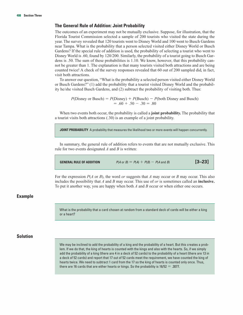
The General Rule of Addition: Joint ProbabilityThe outcomes of an experiment may not be mutually exclusive. Suppose, for illustration, that theFlorida Tourist Commission selected a sample of 200 tourists who visited the state during theyear. The survey revealed that 120 tourists went to Disney World and 100 went to Busch Gardensnear Tampa. What is the probability that a person selected visited either Disney World or BuschGardens? If the special rule of addition is used, the probability of selecting a tourist who went toDisney World is .60, found by 120/200. Similarly, the probability of a tourist going to Busch Gar-dens is .50. The sum of these probabilities is 1.10. We know, however, that this probability can-not be greater than 1. The explanation is that many tourists visited both attractions and are beingcounted twice! A check of the survey responses revealed that 60 out of 200 sampled did, in fact,visit both attractions.
To answer our question, “What is the probability a selected person visited either Disney Worldor Busch Gardens?” (1) add the probability that a tourist visited Disney World and the probabil-ity he/she visited Busch Gardens, and (2) subtract the probability of visiting both. Thus:
P(Disney or Busch) � P(Disney) � P(Busch) � P(both Disney and Busch)� .60 � .50 � .30 � .80
When two events both occur, the probability is called a joint probability. The probability thata tourist visits both attractions (.30) is an example of a joint probability.
In summary, the general rule of addition refers to events that are not mutually exclusive. Thisrule for two events designated A and B is written:
For the expression P(A or B), the word or suggests that A may occur or B may occur. This alsoincludes the possibility that A and B may occur. This use of or is sometimes called an inclusive.To put it another way, you are happy when both A and B occur or when either one occurs.
Example
Solution
We may be inclined to add the probability of a king and the probability of a heart. But this creates a prob-lem. If we do that, the king of hearts is counted with the kings and also with the hearts. So, if we simplyadd the probability of a king (there are 4 in a deck of 52 cards) to the probability of a heart (there are 13 ina deck of 52 cards) and report that 17 out of 52 cards meet the requirement, we have counted the king ofhearts twice. We need to subtract 1 card from the 17 so the king of hearts is counted only once. Thus,there are 16 cards that are either hearts or kings. So the probability is 16/52 � .3077.
What is the probability that a card chosen at random from a standard deck of cards will be either a kingor a heart?
GENERAL RULE OF ADDITION P(A or B) � P(A) � P(B) � P(A and B) [3–23]
JOINT PROBABILITY A probability that measures the likelihood two or more events will happen concurrently.
408 Section Three
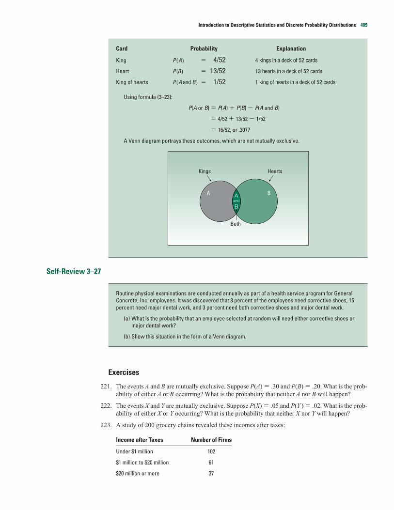
Card Probability Explanation
King P ( A ) � 4/52 4 kings in a deck of 52 cards
Heart P (B ) � 13/52 13 hearts in a deck of 52 cards
King of hearts P ( A and B ) � 1/52 1 king of hearts in a deck of 52 cards
Using formula (3–23):
P(A or B) � P(A) � P(B) � P(A and B)
� 4/52 � 13/52 � 1/52
� 16/52, or .3077
A Venn diagram portrays these outcomes, which are not mutually exclusive.
Self-Review 3–27
Exercises
221. The events A and B are mutually exclusive. Suppose P(A) � .30 and P(B) � .20. What is the prob-ability of either A or B occurring? What is the probability that neither A nor B will happen?
222. The events X and Y are mutually exclusive. Suppose P(X) � .05 and P(Y ) � .02. What is the prob-ability of either X or Y occurring? What is the probability that neither X nor Y will happen?
223. A study of 200 grocery chains revealed these incomes after taxes:
Income after Taxes Number of Firms
Under $1 million 102
$1 million to $20 million 61
$20 million or more 37
Routine physical examinations are conducted annually as part of a health service program for GeneralConcrete, Inc. employees. It was discovered that 8 percent of the employees need corrective shoes, 15percent need major dental work, and 3 percent need both corrective shoes and major dental work.
(a) What is the probability that an employee selected at random will need either corrective shoes ormajor dental work?
(b) Show this situation in the form of a Venn diagram.
Kings Hearts
Both
A B Aand
B
Introduction to Descriptive Statistics and Discrete Probability Distributions 409

a. What is the probability a particular chain has under $1 million in income after taxes?
b. What is the probability a grocery chain selected at random has either an income between $1 mil-lion and $20 million, or an income of $20 million or more? What rule of probability was applied?
224. A study of the opinions of designers with respect to the primary color most desirable for use inexecutive offices showed:
Primary Color Number of Opinions Primary Color Number of Opinions
Red 92 Blue 37
Orange 86 Indigo 46
Yellow 46 Violet 2
Green 91
a. What is the experiment?
b. What is one possible event?
c. What is the probability of selecting a particular response and discovering that the designerprefers red or green?
d. What is the probability that a designer does not prefer yellow?
225. The chair of the board of directors says, “There is a 50% chance this company will earn a profit, a30% chance it will break even, and a 20% chance it will lose money next quarter.”
a. Use an addition rule to find the probability they will not lose money next quarter.
b. Use the complement rule to find the probability they will not lose money next quarter.
226. Suppose the probability you will get a grade of A in this class is .25 and the probability you willget a B is .50. What is the probability your grade will be above C?
227. A single die is rolled. Let A be the event “the die shows 4,” B be the event “the die shows an evennumber,” and C be the event “the die shows an odd number.” Consider each pair of these events anddescribe whether they are mutually exclusive. Then identify whether they are complementary.
228. Two coins are tossed. If A is the event “two heads” and B is the event “two tails,” are A and B mutu-ally exclusive? Are they complements?
229. The probabilities of the events A and B are .20 and .30, respectively. The probability that both A andB occur is .15. What is the probability of either A or B occurring?
230. Let P(X) � .55 and P(Y ) � .35. Assume the probability that they both occur is .20. What is theprobability of either X or Y occurring?
231. Suppose the two events A and B are mutually exclusive. What is the probability of their jointoccurrence?
232. A student is taking two courses, history and math. The probability the student will pass the historycourse is .60, and the probability of passing the math course is .70. The probability of passing bothis .50. What is the probability of passing at least one?
233. A survey of top executives revealed that 35 percent of them regularly read Time magazine, 20 per-cent read Newsweek, and 40 percent read U.S. News and World Report. Ten percent read both Timeand U.S. News and World Report.
a. What is the probability that a particular top executive reads either Time or U.S. News and WorldReport regularly?
b. What is the probability .10 called?
c. Are the events mutually exclusive? Explain.
410 Section Three
234. A study by the National Park Service revealed that 50 percent of vacationers going to the RockyMountain region visit Yellowstone Park, 40 percent visit the Tetons, and 35 percent visit both.
a. What is the probability a vacationer will visit at least one of these attractions?
b. What is the probability .35 called?
c. Are the events mutually exclusive? Explain.
Rules of MultiplicationSpecial Rule of Multiplication The special rule of multiplication requires that two events A andB be independent. Two events are independent if the occurrence of one does not alter the prob-ability of the other. So if the events A and B are independent, the occurrence of A does not alterthe probability of B.
For two independent events A and B, the probability that A and B will both occur is found bymultiplying the two probabilities. This is the special rule of multiplication and is written sym-bolically as:
This rule for combining probabilities presumes that a second event is not affected by the firstevent. To illustrate what is meant by independence of events, suppose two coins are tossed. Theoutcome of one coin (head or tail) is unaffected by the outcome of the other coin (head or tail).To put it another way, two events are independent if the outcome of the second event does notdepend on the outcome of the first event.
For three independent events A, B, and C, the special rule of multiplication used to determinethe probability that all three events will occur is:
P(A and B and C) � P(A)P(B)P(C)
Example
Solution
The probability the first member made an airline reservation last year is .60, written P(R1) � .60, where R1
refers to the fact that the first member made a reservation. The probability that the second memberselected made a reservation is also .60, so P(R2) � .60. Since the number of AAA members is very large,you may assume that R1 and R2 are independent. Consequently, using formula 3–24, the probability theyboth make a reservation is .36, found by:
P(R1 and R2) � P(R1)P(R2) � (.60)(.60) � .36
A survey by the American Automobile Association (AAA) revealed 60 percent of its members made air-line reservations last year. Two members are selected at random. What is the probability both made air-line reservations last year?
SPECIAL RULE OF MULTIPLICATION P(A and B) � P(A)P(B) [3–24]
INDEPENDENT The occurrence of one event has no effect on the probability of the occurrence of any other event.
Introduction to Descriptive Statistics and Discrete Probability Distributions 411

All possible outcomes can be shown as follows. R means a reservation is made, and NR means noreservation was made.
R R
or R NR
or NR R
or NR NR
Self-Review 3–28
If two events are not independent, they are referred to as dependent. To illustrate dependency,suppose there are 10 rolls of film in a box, and it is known that 3 are defective. A roll of film isselected from the box. Obviously, the probability of selecting a defective roll is 3⁄10, and the proba-bility of selecting a good roll is 7⁄10. Then a second roll is selected from the box without the first onebeing returned to the box. The probability this second roll is defective depends on whether the firstroll selected was defective or good. The probability that the second roll is defective is:
2⁄9, if the first roll was defective. (Only two defective rolls remain in the box containingnine rolls.)
3⁄9, if the first roll selected was good. (All three defective rolls are still in the boxcontaining nine rolls.)
The fraction 2⁄9 (or 3⁄9) is aptly called a conditional probability because its value is conditionalon (dependent on) whether a defective or a good roll of film is chosen in the first selection fromthe box.
General Rule of Multiplication We use the general rule of multiplication to find the joint prob-ability that two events will occur, such as selecting 2 defective rolls from the box of 10 rolls, oneafter the other. In general, the rule states that for two events A and B, the joint probability that bothevents will happen is found by multiplying the probability event A will happen by the conditionalprobability of event B occurring. Symbolically, the joint probability P(A and B) is found by:
CONDITIONAL PROBABILITY The probability of a particular event occurring, given that another event has occurred.
1. From long experience, Teton Tire knows the probability is .80 that their XB-70 will last 60,000 milesbefore it becomes bald or fails. An adjustment is made on any tire that does not last 60,000 miles. Youpurchase four XB-70s. What is the probability all four tires will last at least 60,000 miles?
2. As cited in an earlier example, an automatic Shaw machine inserts mixed vegetables into a plasticbag. Past experience revealed some packages were underweight and some overweight, but most ofthem had satisfactory weight.
Weight Probability
Underweight .025
Satisfactory .900
Overweight .075
(a) What is the probability of selecting three packages from the food processing line today and findingall three of them are underweight?
(b) What does this probability mean?
412 Section Three

where P(B � A) stands for the probability B will occur given that A has already occurred. The ver-tical line means “given that.”
Example
Solution
The first roll of film selected from the box being found defective is event A. P(A) � 3⁄10 because 3 out ofthe 10 are defective. The second roll selected being found defective is event B. Therefore, P(B � A) � 2⁄9,because after the first selection was found to be defective, only 2 defective rolls of film remained in thebox containing 9 rolls. Determining the probability of two defectives [see formula (3–25 )]:
P(A and B) � P(A)P(B � A) � � or about .07
Incidentally, it is assumed that this experiment was conducted without replacement—that is, the firstdefective roll of film was not thrown back in the box before the next roll was selected. It should also benoted that the general rule of multiplication can be extended to more than two events. For three events,A, B, and C, the formula would be:
P(A and B and C) � P(A)P(B � A)P(C � A and B)
For illustration, the probability the first three rolls chosen from the box will all be defective is .00833,found by:
P(A and B and C) � P(A)P(B � A)P(C � A and B)
� � � .00833
Self-Review 3–29
Another application of the general rule of multiplication follows. A survey of executives dealtwith their loyalty to the company. One of the questions was, “If you were given an offer byanother company equal to or slightly better than your present position, would you remain with thecompany or take the other position?” The responses of the 200 executives in the survey werecross-classified with their length of service with the company. (See Exhibit 3–41.) The type oftable that resulted is usually referred to as a contingency table.
The board of directors of Tarbell Industries consists of eight men and four women. A four-member searchcommittee is to be chosen at random to recommend a new company president.
(a) What is the probability all four members of the search committee will be women?
(b) What is the probability all four members will be men?
(c) Does the sum of the probabilities for the events described in parts (a) and ( b) equal 1? Explain.
6720� 3
10��29��18�
690� 3
10��29�
To illustrate the formula, let’s use the problem with 10 rolls of film in a box, 3 of which are defective. Tworolls are to be selected, one after the other. What is the probability of selecting a defective roll followedby another defective roll?
GENERAL RULE OF MULTIPLICATION P(A and B) � P(A)P(B � A) [3–25]
Introduction to Descriptive Statistics and Discrete Probability Distributions 413

EXHIBIT 3–41 Loyalty of Executives and Length of Service with Company
Length of ServiceLess than 1–5 6–10 More than
Loyalty 1 Year Years Years 10 Years Total
Would remain 10 30 5 75 120
Would not remain 25 15 10 30 80
200
Example
Solution
Note that two events occur at the same time—the executive would remain with the company, and he orshe has more than 10 years of service.
1. Event A happens if a randomly selected executive will remain with the company despite an equal orslightly better offer from another company. To find the probability that event A will happen, refer toExhibit 3–41. Note that there are 120 executives out of the 200 in the survey who would remain with thecompany, so P(A) � 120/200, or .60.
2. Event B4 happens if a randomly selected executive has more than 10 years of service with the com-pany. Thus, P(B4 � A) is the conditional probability that an executive with more than 10 years of servicewould remain with the company despite an equal or slightly better offer from another company. Refer-ring to the contingency table, Exhibit 3–41, 75 of the 120 executives who would remain have more than10 years of service, so P(B4 � A) � 75/120.
Solving for the probability that an executive randomly selected will be one who would remain with thecompany and who has more than 10 years of service with the company, using the general rule of multipli-cation in formula (3–25):
P(A and B4) � P(A)P(B4 � A) � � � .375
Self-Review 3–30
Tree DiagramsThe tree diagram is a graph that is helpful in organizing calculations that involve several stages.Each segment in the tree is one stage of the problem. The branches of a tree diagram are weightedby probabilities. We will use the data in Exhibit 3–42 to show the construction of a tree diagram.
1. To construct a tree diagram, we begin by drawing a heavy dot on the left to represent the root of thetree (see Exhibit 3–42).
Refer to Exhibit 3–41. Using the general rule of multiplication, what is the probability of selecting at ran-dom an executive who would not remain with the company and has less than one year of service?
9,00024,000�120
200�� 75120�
What is the probability of randomly selecting an executive who is loyal to the company (would remain)and who has more than 10 years of service?
414 Section Three
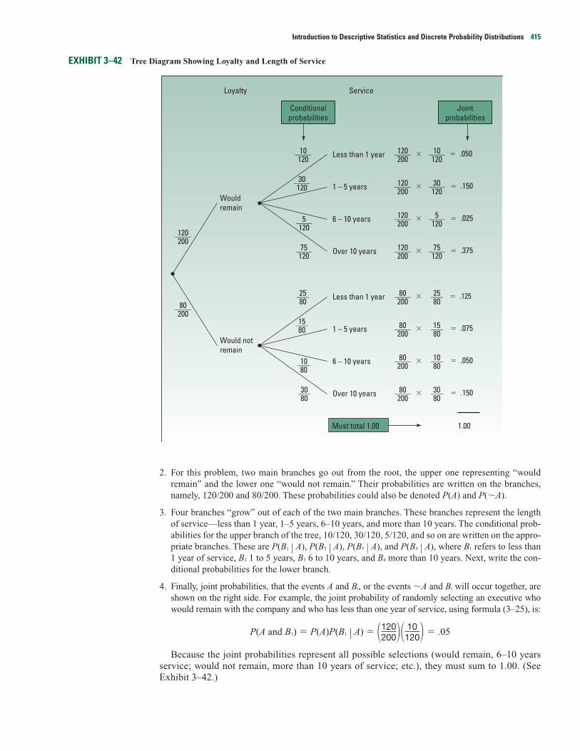
EXHIBIT 3–42 Tree Diagram Showing Loyalty and Length of Service
2. For this problem, two main branches go out from the root, the upper one representing “wouldremain” and the lower one “would not remain.” Their probabilities are written on the branches,namely, 120/200 and 80/200. These probabilities could also be denoted P(A) and P(�A).
3. Four branches “grow” out of each of the two main branches. These branches represent the lengthof service—less than 1 year, 1–5 years, 6–10 years, and more than 10 years. The conditional prob-abilities for the upper branch of the tree, 10/120, 30/120, 5/120, and so on are written on the appro-priate branches. These are P(B1 � A), P(B2 � A), P(B3 � A), and P(B4 � A), where B1 refers to less than1 year of service, B2 1 to 5 years, B3 6 to 10 years, and B4 more than 10 years. Next, write the con-ditional probabilities for the lower branch.
4. Finally, joint probabilities, that the events A and Bi, or the events �A and Bi will occur together, areshown on the right side. For example, the joint probability of randomly selecting an executive whowould remain with the company and who has less than one year of service, using formula (3–25), is:
P(A and B1) � P(A)P(B1 � A) � � .05
Because the joint probabilities represent all possible selections (would remain, 6–10 yearsservice; would not remain, more than 10 years of service; etc.), they must sum to 1.00. (SeeExhibit 3–42.)
�120200�� 10
120�
10 ____ 120 Less than 1 year
1 – 5 years
6 – 10 years
Over 10 years
120 ____ 200
� � .050
� � .150
� � .025
� � .375
10 ____ 120
30 ____ 120 120 ____
20030 ____
120
5 ____ 120
120 ____ 200
5 ____ 120
75 ____ 120
120 ____ 200
75 ____ 120
25 ___ 80 Less than 1 year
1 – 5 years
6 – 10 years
Over 10 years
80 ____ 200
� � .125
� � .075
� � .050
� � .150
25 ___ 80
15 ___ 80 80 ____
20015 ___ 80
10 ___ 80
80 ____ 200
10 ___ 80
30 ___ 80
80 ____ 200
30 ___ 80
1.00Must total 1.00
Joint probabilities
Conditionalprobabilities
ServiceLoyalty
Would remain
Would not remain
120 ____ 200
80 ____ 200
Introduction to Descriptive Statistics and Discrete Probability Distributions 415
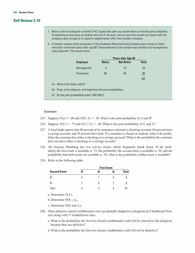
Self-Review 3–31
Exercises
235. Suppose P(A) � .40 and P(B � A) � .30. What is the joint probability of A and B?
236. Suppose P(X1) � .75 and P(Y2 � X1) � .40. What is the joint probability of X1 and Y2?
237. A local bank reports that 80 percent of its customers maintain a checking account, 60 percent havea savings account, and 50 percent have both. If a customer is chosen at random, what is the proba-bility the customer has either a checking or a savings account? What is the probability the customerdoes not have either a checking or a savings account?
238. All Seasons Plumbing has two service trucks which frequently break down. If the prob-ability the first truck is available is .75, the probability the second truck is available is .50, and theprobability that both trucks are available is .30, what is the probability neither truck is available?
239. Refer to the following table.
First EventSecond Event A1 A2 A3 Total
B1 2 1 3 6
B2 1 2 1 4
Total 3 3 4 10
a. Determine P(A1).
b. Determine P(B1 � A2).
c. Determine P(B2 and A3).
240. Three defective electric toothbrushes were accidentally shipped to a drugstore by Cleanbrush Prod-ucts along with 17 nondefective ones.
a. What is the probability the first two electric toothbrushes sold will be returned to the drugstorebecause they are defective?
b. What is the probability the first two electric toothbrushes sold will not be defective?
1. Refer to the tree diagram in Exhibit 3–42. Explain the path you would follow to find the joint probabilityof selecting an executive at random who has 6–10 years’ service and who would not remain with thecompany upon receipt of an equal or slightly better offer from another company.
2. A random sample of the employees of the Hardware Manufacturing Company was chosen to deter-mine their retirement plans after age 65. Those selected in the sample were divided into managementand production. The results were:
Plans after Age 65Employee Retire Not Retire Total
Management 5 15 20
Production 30 50 80
100
(a) What is the table called?
(b) Draw a tree diagram, and determine the joint probabilities.
(c) Do the joint probabilities total 1.00? Why?
416 Section Three
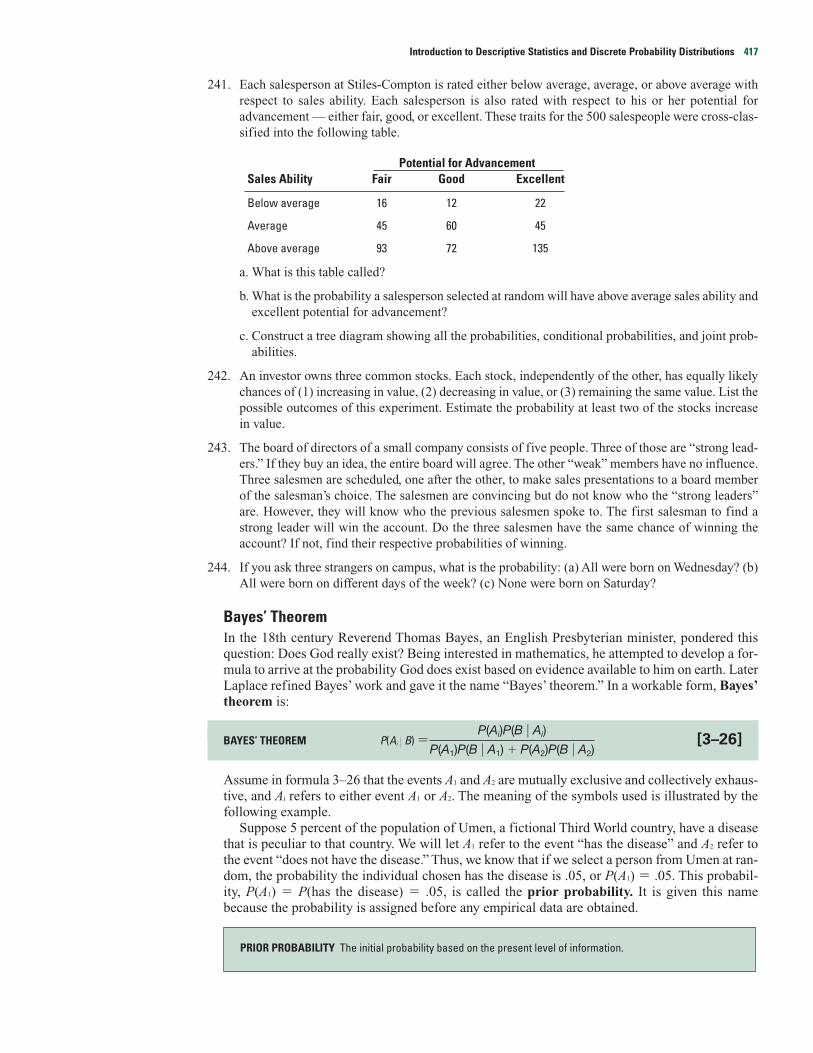
241. Each salesperson at Stiles-Compton is rated either below average, average, or above average withrespect to sales ability. Each salesperson is also rated with respect to his or her potential foradvancement — either fair, good, or excellent. These traits for the 500 salespeople were cross-clas-sified into the following table.
Potential for AdvancementSales Ability Fair Good Excellent
Below average 16 12 22
Average 45 60 45
Above average 93 72 135
a. What is this table called?
b. What is the probability a salesperson selected at random will have above average sales ability andexcellent potential for advancement?
c. Construct a tree diagram showing all the probabilities, conditional probabilities, and joint prob-abilities.
242. An investor owns three common stocks. Each stock, independently of the other, has equally likelychances of (1) increasing in value, (2) decreasing in value, or (3) remaining the same value. List thepossible outcomes of this experiment. Estimate the probability at least two of the stocks increasein value.
243. The board of directors of a small company consists of five people. Three of those are “strong lead-ers.” If they buy an idea, the entire board will agree. The other “weak” members have no influence.Three salesmen are scheduled, one after the other, to make sales presentations to a board memberof the salesman’s choice. The salesmen are convincing but do not know who the “strong leaders”are. However, they will know who the previous salesmen spoke to. The first salesman to find astrong leader will win the account. Do the three salesmen have the same chance of winning theaccount? If not, find their respective probabilities of winning.
244. If you ask three strangers on campus, what is the probability: (a) All were born on Wednesday? (b)All were born on different days of the week? (c) None were born on Saturday?
Bayes’ TheoremIn the 18th century Reverend Thomas Bayes, an English Presbyterian minister, pondered thisquestion: Does God really exist? Being interested in mathematics, he attempted to develop a for-mula to arrive at the probability God does exist based on evidence available to him on earth. LaterLaplace refined Bayes’ work and gave it the name “Bayes’ theorem.” In a workable form, Bayes’theorem is:
BAYES’ THEOREM P(Ai � B) � [3–26]
Assume in formula 3–26 that the events A1 and A2 are mutually exclusive and collectively exhaus-tive, and Ai refers to either event A1 or A2. The meaning of the symbols used is illustrated by thefollowing example.
Suppose 5 percent of the population of Umen, a fictional Third World country, have a diseasethat is peculiar to that country. We will let A1 refer to the event “has the disease” and A2 refer tothe event “does not have the disease.” Thus, we know that if we select a person from Umen at ran-dom, the probability the individual chosen has the disease is .05, or P(A1) � .05. This probabil-ity, P(A1) � P(has the disease) � .05, is called the prior probability. It is given this namebecause the probability is assigned before any empirical data are obtained.
PRIOR PROBABILITY The initial probability based on the present level of information.
P(Ai)P(B � Ai)
P(A1)P(B � A1) � P(A2)P(B � A2)
Introduction to Descriptive Statistics and Discrete Probability Distributions 417
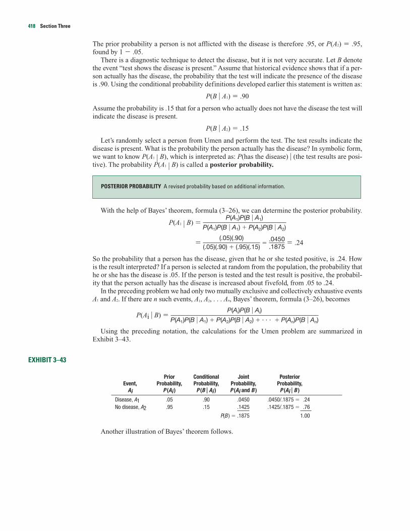
The prior probability a person is not afflicted with the disease is therefore .95, or P(A2) � .95,found by 1 � .05.
There is a diagnostic technique to detect the disease, but it is not very accurate. Let B denotethe event “test shows the disease is present.” Assume that historical evidence shows that if a per-son actually has the disease, the probability that the test will indicate the presence of the diseaseis .90. Using the conditional probability definitions developed earlier this statement is written as:
P(B � A1) � .90
Assume the probability is .15 that for a person who actually does not have the disease the test willindicate the disease is present.
P(B � A2) � .15
Let’s randomly select a person from Umen and perform the test. The test results indicate thedisease is present. What is the probability the person actually has the disease? In symbolic form,we want to know P(A1 � B), which is interpreted as: P(has the disease) � (the test results are posi-tive). The probability P(A1 � B) is called a posterior probability.
With the help of Bayes’ theorem, formula (3–26), we can determine the posterior probability.
P(A1 � B) �
� � � .24
So the probability that a person has the disease, given that he or she tested positive, is .24. Howis the result interpreted? If a person is selected at random from the population, the probability thathe or she has the disease is .05. If the person is tested and the test result is positive, the probabil-ity that the person actually has the disease is increased about fivefold, from .05 to .24.
In the preceding problem we had only two mutually exclusive and collectively exhaustive eventsA1 and A2. If there are n such events, A1, A2, . . . An, Bayes’ theorem, formula (3–26), becomes
P(Ai � B) �
Using the preceding notation, the calculations for the Umen problem are summarized inExhibit 3–43.
EXHIBIT 3–43
Prior Conditional Joint PosteriorEvent, Probability, Probability, Probability, Probability,
Ai P (Ai ) P (B � Ai ) P (Ai and B ) P (Ai � B )
Disease, A1 .05 .90 .0450 .0450/.1875 � .24No disease, A2 .95 .15 .1425 .1425/.1875 � .76
P(B ) � .1875 1.00
Another illustration of Bayes’ theorem follows.
P(Ai)P(B � Ai)
P(A1)P(B � A1) � P(A2)P(B � A2) � · · · � P(An)P(B � An)
.0450
.1875(.05)(.90)
(.05)(.90) � (.95)(.15)
P(A1)P(B � A1)
P(A1)P(B � A1) � P(A2)P(B � A2)
POSTERIOR PROBABILITY A revised probability based on additional information.
418 Section Three
Snapshot 3–9A recent study by the National Collegiate Athletic Association (NCAA) reported that of 150,000 senior boys playing on their high school basketballteam, 64 would make a professional team. To put it another way, the odds of a high school senior basketball player making a professional team are1 in 2,344. From the same study:
1. The odds of a high school senior playing some college basketball are about 1 in 40.
2. The odds of a high school senior playing college basketball as a senior in college are about 1 in 60.
3. If you play as a senior in college, the odds of making a professional team are about 1 in 37.5.
Example
Solution
As a first step, let’s summarize some of the information given in the problem statement.
• There are three mutually exclusive and collectively exhaustive events, that is, three suppliers.
A1 The LS-24 was purchased from Hall Electronics
A2 The LS-24 was purchased from Schuller Sales
A3 The LS-24 was purchased from Crawford Components
• The prior probabilities are:
P(A1) � .30 The probability the LS-24 was manufactured by Hall Electronics
P(A2) � .20 The probability the LS-24 was manufactured by Schuller Sales
P(A3) � .50 The probability the LS-24 was manufactured by Crawford Components
• The additional information can be either:
B1 The LS-24 appears defective, or
B2 The LS-24 appears not to be defective.
• The following conditional probabilities are given.
P(B1 � A1) � .03 The probability that an LS-24 chip produced by Hall Electronics is defective
P(B1 � A2) � .05 The probability that an LS-24 chip produced by Schuller Sales is defective
P(B1 � A3) � .04 The probability that an LS-24 chip produced by Crawford Components is defective
A manufacturer of VCRs purchases a particular microchip, called the LS-24, from three suppliers: HallElectronics, Schuller Sales, and Crawford Components. Thirty percent of the LS-24 chips are purchasedfrom Hall Electronics, 20 percent from Schuller Sales, and the remaining 50 percent from Crawford Com-ponents. The manufacturer has extensive histories on the three suppliers and knows that 3 percent of theLS-24 chips from Hall Electronics are defective, 5 percent of chips from Schuller Sales are defective, and4 percent of the chips purchased from Crawford Components are defective.
When the LS-24 chips arrive at the manufacturer, they are placed directly in a bin and not inspectedor otherwise identified by supplier. A worker selects a chip for installation in a VCR and finds it defective.What is the probability that it was manufactured by Schuller Sales?
Introduction to Descriptive Statistics and Discrete Probability Distributions 419
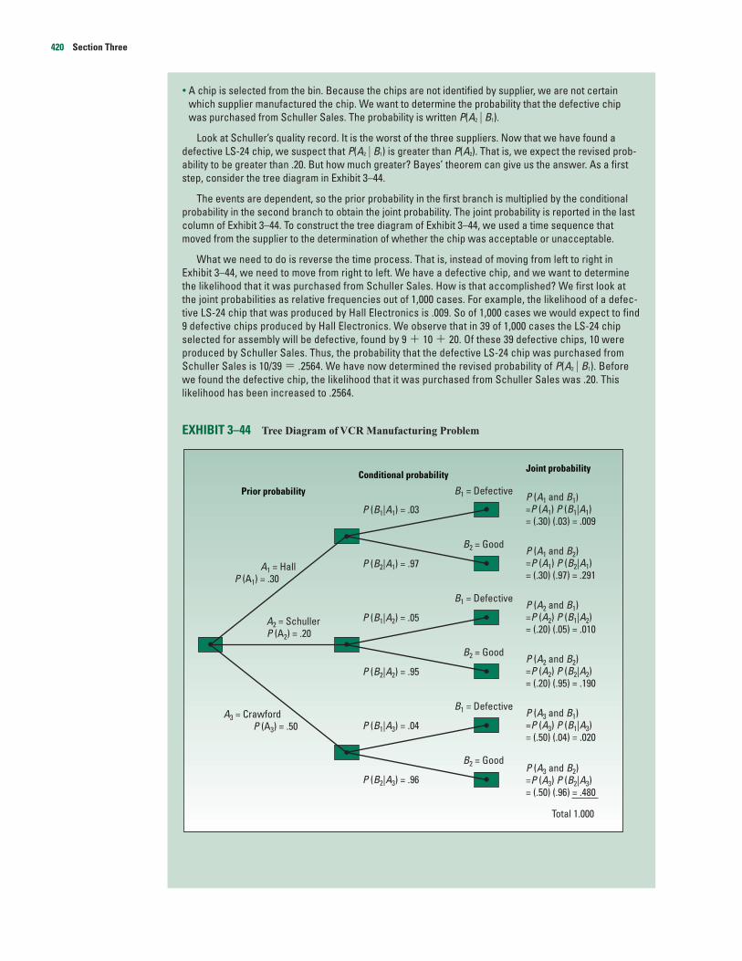
• A chip is selected from the bin. Because the chips are not identified by supplier, we are not certainwhich supplier manufactured the chip. We want to determine the probability that the defective chipwas purchased from Schuller Sales. The probability is written P(A2 � B1).
Look at Schuller’s quality record. It is the worst of the three suppliers. Now that we have found adefective LS-24 chip, we suspect that P(A2 � B1) is greater than P(A2). That is, we expect the revised prob-ability to be greater than .20. But how much greater? Bayes’ theorem can give us the answer. As a firststep, consider the tree diagram in Exhibit 3–44.
The events are dependent, so the prior probability in the first branch is multiplied by the conditionalprobability in the second branch to obtain the joint probability. The joint probability is reported in the lastcolumn of Exhibit 3–44. To construct the tree diagram of Exhibit 3–44, we used a time sequence thatmoved from the supplier to the determination of whether the chip was acceptable or unacceptable.
What we need to do is reverse the time process. That is, instead of moving from left to right inExhibit 3–44, we need to move from right to left. We have a defective chip, and we want to determinethe likelihood that it was purchased from Schuller Sales. How is that accomplished? We first look atthe joint probabilities as relative frequencies out of 1,000 cases. For example, the likelihood of a defec-tive LS-24 chip that was produced by Hall Electronics is .009. So of 1,000 cases we would expect to find9 defective chips produced by Hall Electronics. We observe that in 39 of 1,000 cases the LS-24 chipselected for assembly will be defective, found by 9 � 10 � 20. Of these 39 defective chips, 10 wereproduced by Schuller Sales. Thus, the probability that the defective LS-24 chip was purchased fromSchuller Sales is 10/39 � .2564. We have now determined the revised probability of P(A2 � B1). Beforewe found the defective chip, the likelihood that it was purchased from Schuller Sales was .20. Thislikelihood has been increased to .2564.
EXHIBIT 3–44 Tree Diagram of VCR Manufacturing Problem
P (A1 and B1)=P (A1) P (B1|A1)= (.30) (.03) = .009
P (A1 and B2)=P (A1) P (B2|A1)= (.30) (.97) = .291
P (A2 and B1)=P (A2) P (B1|A2)= (.20) (.05) = .010
P (A2 and B2)=P (A2) P (B2|A2)= (.20) (.95) = .190
P (A3 and B1)=P (A3) P (B1|A3)= (.50) (.04) = .020
P (A3 and B2)=P (A3) P (B2|A3)= (.50) (.96) = .480
Total 1.000
B1 = Defective
B2 = Good
B1 = Defective
B2 = Good
B1 = Defective
B2 = Good
P (B1|A1) = .03
P (B2|A1) = .97
P (B1|A2) = .05
P (B2|A2) = .95
P (B1|A3) = .04
P (B2|A3) = .96
A2 = SchullerP (A2) = .20
A1 = HallP (A1) = .30
A3 = CrawfordP (A3) = .50
Joint probabilityConditional probability
Prior probability
420 Section Three
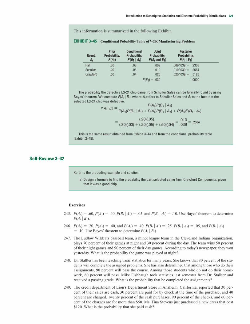
This information is summarized in the following Exhibit.
EXHIBIT 3–45 Conditional Pobability Table of VCR Manfacturing Problem
Prior Conditional Joint PosteriorEvent, Probability, Probability, Probability, Probability,
Ai P (Ai ) P (B1 � Ai ) P (Ai and B1) P(Ai � B1)
Hall .30 .03 .009 .009/.039 � .2308Schuller .20 .05 .010 .010/.039 � .2564Crawford .50 .04 .020 .020/.039 � .5128
P (B1) � .039 1.0000
The probability the defective LS-24 chip came from Schuller Sales can be formally found by usingBayes’ theorem. We compute P(A2 � B1), where A2 refers to Schuller Sales and B1 to the fact that theselected LS-24 chip was defective.
P(A2 � B1) �
� � � .2564
This is the same result obtained from Exhibit 3–44 and from the conditional probability table (Exhibit 3–45).
Self-Review 3–32
Exercises
245. P(A1) � .60, P(A2) � .40, P(B1 � A1) � .05, and P(B1 � A2) � .10. Use Bayes’ theorem to determineP(A1 � B1).
246. P(A1) � .20, P(A2) � .40, and P(A3) � .40. P(B1 � A1) � .25. P(B1 � A2) � .05, and P(B1 � A3) � .10. Use Bayes’ theorem to determine P(A3 � B1).
247. The Ludlow Wildcats baseball team, a minor league team in the Cleveland Indians organization,plays 70 percent of their games at night and 30 percent during the day. The team wins 50 percentof their night games and 90 percent of their day games. According to today’s newspaper, they wonyesterday. What is the probability the game was played at night?
248. Dr. Stallter has been teaching basic statistics for many years. She knows that 80 percent of the stu-dents will complete the assigned problems. She has also determined that among those who do theirassignments, 90 percent will pass the course. Among those students who do not do their home-work, 60 percent will pass. Mike Fishbaugh took statistics last semester from Dr. Stallter andreceived a passing grade. What is the probability that he completed the assignments?
249. The credit department of Lion’s Department Store in Anaheim, California, reported that 30 per-cent of their sales are cash, 30 percent are paid for by check at the time of the purchase, and 40percent are charged. Twenty percent of the cash purchases, 90 percent of the checks, and 60 per-cent of the charges are for more than $50. Ms. Tina Stevens just purchased a new dress that cost$120. What is the probability that she paid cash?
Refer to the preceding example and solution.
(a) Design a formula to find the probability the part selected came from Crawford Components, giventhat it was a good chip.
.010
.039(.20)(.05)
(.30)(.03) � (.20)(.05) � (.50)(.04)
P(A2)P(B1 � A2)
P(A1)P(B1 � A1) � P(A2)P(B1 � A2) � P(A3)P(B1 � A3)
Introduction to Descriptive Statistics and Discrete Probability Distributions 421
250. One-fourth of the residents of the Burning Ridge Estates leave their garage doors open when theyare away from home. The local chief of police estimates that 5 percent of the garages with opendoors will have something stolen, but only 1 percent of those closed will have something stolen. Ifa garage is robbed, what is the probability the doors were left open?
Principles of CountingIf the number of possible outcomes in an experiment is small, it is relatively easy to count them.There are six possible outcomes, for example, resulting from the roll of a die, namely:
If, however, there are a large number of possible outcomes, such as the number of boys and girlsfor families with 10 children, it would be tedious to count all the possibilities. They could haveall boys, one boy and nine girls, two boys and eight girls, and so on. To facilitate counting, threecounting formulas will be examined: the multiplication formula (not to be confused with themultiplication rule described earlier), the permutation formula, and the combination formula.
The Multiplication Formula
In terms of a formula:
This can be extended to more than two events. For three events m, n, and o:
Total number of arrangements � (m)(n)(o)
Example
Solution
Of course the dealer could determine the total number of arrangements by picturing and counting them.There are six.
We can employ the multiplication formula as a check (where m is the number of models and n thewheel cover type). Using formula (3–27):
Total possible arrangements � (m)(n) � (3)(2) � 6
An automobile dealer wants to advertise that for $29,999 you can buy a convertible, a two-door, or a four-door model with your choice of either wire wheel covers or solid wheel covers. How many differentarrangements of models and wheel covers can the dealer offer?
MULTIPLICATION FORMULA Total number of arrangements � (m)(n) [3–27]
MULTIPLICATION FORMULA If there are m ways of doing one thing and n ways of doing another thing, there arem � n ways of doing both.
422 Section Three
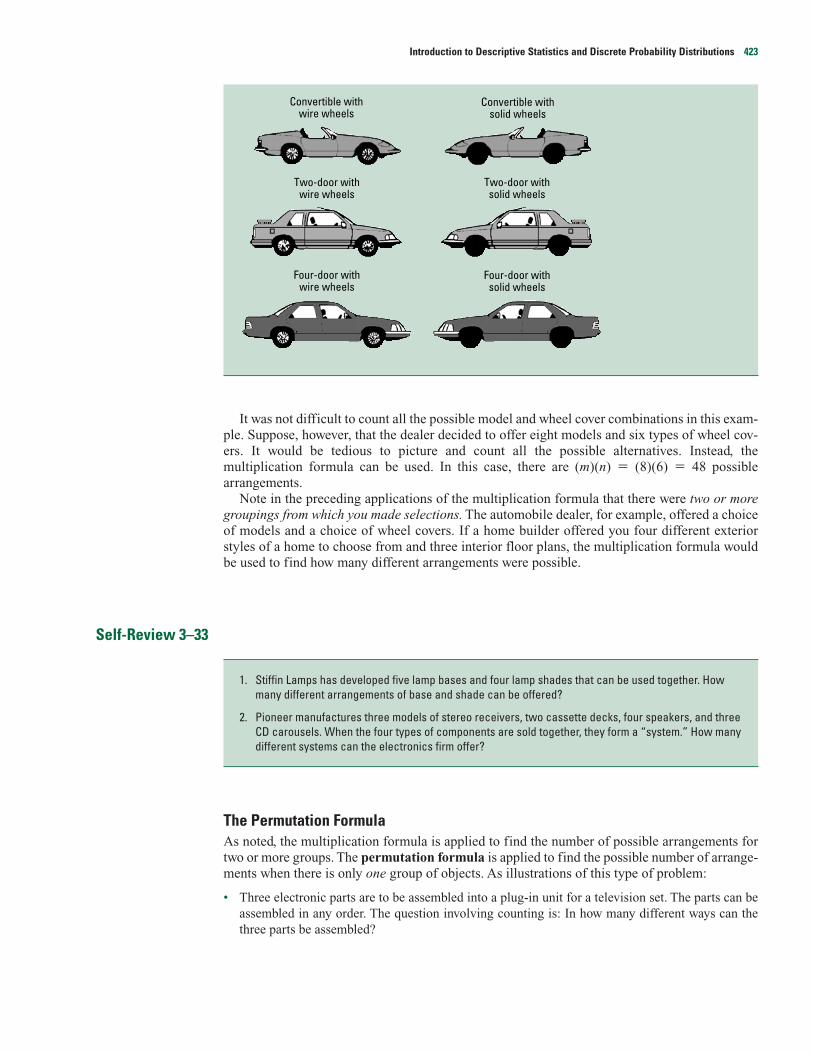
It was not difficult to count all the possible model and wheel cover combinations in this exam-ple. Suppose, however, that the dealer decided to offer eight models and six types of wheel cov-ers. It would be tedious to picture and count all the possible alternatives. Instead, themultiplication formula can be used. In this case, there are (m)(n) � (8)(6) � 48 possiblearrangements.
Note in the preceding applications of the multiplication formula that there were two or moregroupings from which you made selections. The automobile dealer, for example, offered a choiceof models and a choice of wheel covers. If a home builder offered you four different exteriorstyles of a home to choose from and three interior floor plans, the multiplication formula wouldbe used to find how many different arrangements were possible.
Self-Review 3–33
The Permutation FormulaAs noted, the multiplication formula is applied to find the number of possible arrangements fortwo or more groups. The permutation formula is applied to find the possible number of arrange-ments when there is only one group of objects. As illustrations of this type of problem:
• Three electronic parts are to be assembled into a plug-in unit for a television set. The parts can beassembled in any order. The question involving counting is: In how many different ways can thethree parts be assembled?
1. Stiffin Lamps has developed five lamp bases and four lamp shades that can be used together. Howmany different arrangements of base and shade can be offered?
2. Pioneer manufactures three models of stereo receivers, two cassette decks, four speakers, and threeCD carousels. When the four types of components are sold together, they form a “system.” How manydifferent systems can the electronics firm offer?
Convertible withwire wheels
Two-door withwire wheels
Convertible withsolid wheels
Four-door withwire wheels
Two-door withsolid wheels
Four-door withsolid wheels
Introduction to Descriptive Statistics and Discrete Probability Distributions 423

• A machine operator must make four safety checks before starting his machine. It does not matterin which order the checks are made. In how many different ways can the operator make the checks?
One order for the first illustration might be: the transistor first, the LEDs second, and the syn-thesizer third. This arrangement is called a permutation.
Note that the arrangements a b c and b a c are different permutations. The formula to count thetotal number of different permutations is:
PERMUTATION FORMULA n Pr � [3–28]
where:
n is the total number of objects.
r is the number of objects selected.
Before we solve the two problems illustrated, note that permutations and combinations (to bediscussed shortly) use a notation called n factorial. It is written n! and means the product of n(n� 1)(n � 2)(n � 3) . . . (1). For instance, 5! � 5 � 4 � 3 � 2 � 1 � 120.
As shown below, numbers can be canceled when the same numbers are included in the numer-ator and denominator.
� � 180
By definition, zero factorial, written 0!, is 1. That is, 0! � 1.
Example
Solution
n � 3 because there are three electronic parts to be assembled. r � 3 because all three are to beinserted in the plug-in unit. Solving using formula (3–28):
nPr � � � � � 6
A check can be made to the number of permutations arrived at using the permutation formula. Tocheck, we merely determine how many “spaces” have to be filled and the possibilities for each “space”and apply the multiplication formula. In the problem involving three electronic parts, there are three loca-tions in the plug-in unit for the three parts. There are three possibilities for the first place, two for the sec-ond (one has been used up), and one for the third, as follows:
(3)(2)(1) � 6 permutations
The six ways in which the three electronic parts, lettered A, B, C, can be arranged are:
ABC BAC CAB ACB BCA CBA
3!1
3!0!
3!(3 � 3)!
n!(n � r)!
Referring to the group of three electronic parts that are to be assembled in any order, in how many differ-ent ways can they be assembled?
6 · 5 · 4� · 3� · 2� · 1�(3 · 2 · 1)4� · 3� · 2� ·1�
6!3!4!
n!(n � r)!
PERMUTATION Any arrangement of r objects selected from a single group of n possible objects.
424 Section Three

In the previous example we selected and arranged all the objects, that is n � r. In many cases,only some objects are selected and arranged from the n possible objects. We explain the detailsof this application in the following example.
Example
Solution
There are eight possibilities for the first available space in the production area, seven for the secondspace (one has been used up), and six for the third space. Thus:
(8)(7)(6) � 336, that is,
there are a total of 336 different possible arrangements. This could also be found using formula 3–28. If n� 8 machines, and r � 3 spaces available, the formula leads to
nPr � � � � � 336
The Combination FormulaIf the order of the selected objects is not important, any selection is called a combination. The for-mula to count the number of r object combinations from a set of n objects is:
COMBINATION FORMULA nCr � [3–29]
For example, if executives Able, Baker, and Chauncy are to be chosen as a committee to negoti-ate a merger, there is only one possible combination of these three; the committee of Able, Baker,and Chauncy is the same as the committee of Baker, Chauncy, and Able. Using the combinationformula:
nCr � � � 1
Example
The marketing department has been given the assignment of designing color codes for the 42 differentlines of compact discs sold by Goody Records. Three colors are to be used on each CD, but a combina-tion of three colors used for one CD cannot be rearranged and used to identify a different CD. This meansthat if green, yellow, and violet were used to identify one line, then yellow, green, and violet (or any othercombination of these three colors) cannot be used to identify another line. Would seven colors takenthree at a time be adequate to color code the 42 lines?
3 · 2 ·13 · 2 · 1(1)
n!r !(n � r)!
n!r !(n � r)!
(8)(7)(6)5!5!
8!5!
8!(8 � 3)!
n!(n � r)!
The Betts Machine Shop, Inc., has eight screw machines but only three spaces available in the produc-tion area for the machines. In how many different ways can the eight machines be arranged in the threespaces available?
Introduction to Descriptive Statistics and Discrete Probability Distributions 425
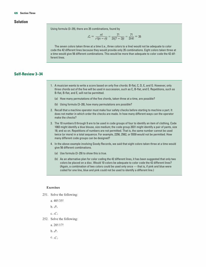
Solution
Using formula (3–29), there are 35 combinations, found by
7C3 � � � � 35
The seven colors taken three at a time (i.e., three colors to a line) would not be adequate to colorcode the 42 different lines because they would provide only 35 combinations. Eight colors taken three ata time would give 56 different combinations. This would be more than adequate to color code the 42 dif-ferent lines.
Self-Review 3–34
Exercises
251. Solve the following:
a. 40!/35!
b. 7P4
c. 5C2
252. Solve the following:
a. 20!/17!
b. 9P3
c. 7C2
1. A musician wants to write a score based on only five chords: B-flat, C, D, E, and G. However, onlythree chords out of the five will be used in succession, such as C, B-flat, and E. Repetitions, such asB-flat, B-flat, and E, will not be permitted.
(a) How many permutations of the five chords, taken three at a time, are possible?
(b) Using formula (3–28), how many permutations are possible?
2. Recall that a machine operator must make four safety checks before starting to machine a part. Itdoes not matter in which order the checks are made. In how many different ways can the operatormake the checks?
3. The 10 numbers 0 through 9 are to be used in code groups of four to identify an item of clothing. Code1083 might identify a blue blouse, size medium; the code group 2031 might identify a pair of pants, size18; and so on. Repetitions of numbers are not permitted. That is, the same number cannot be usedtwice (or more) in a total sequence. For example, 2256, 2562, or 5559 would not be permitted. Howmany different code groups can be designed?
4. In the above example involving Goody Records, we said that eight colors taken three at a time wouldgive 56 different combinations.
(a) Use formula (3–29) to show this is true.
(b) As an alternative plan for color coding the 42 different lines, it has been suggested that only twocolors be placed on a disc. Would 10 colors be adequate to color code the 42 different lines?(Again, a combination of two colors could be used only once — that is, if pink and blue werecoded for one line, blue and pink could not be used to identify a different line.)
7!3!4!
7!3!(7 � 3)!
n!r !(n � r)!
426 Section Three

253.A pollster randomly selected 4 of 10 available people. How many different groups of 4 are possible?
254. A telephone number consists of seven digits, the first three representing the exchange. How manydifferent telephone numbers are possible within the 537 exchange?
255. An overnight express company must include five cities on its route. How many different routes arepossible, assuming that it does not matter in which order the cities are included in the routing?
256. A representative of the Environmental Protection Agency (EPA) wants to select samples from 10landfills. The director has 15 landfills from which she can collect samples. How many differentsamples are possible?
257. A national pollster has developed 15 questions designed to rate the performance of the Presidentof the United States. The pollster will select 10 of these questions. How many different arrange-ments are there for the order of the 10 selected questions?
258. A company is creating three new divisions and seven managers are eligible to be appointed headof a division. How many different ways could the three new heads be appointed?
Summary
I. A probability is a value between 0 and 1 inclusive that represents the likelihood a particular eventwill happen.
A. An experiment is the observation of some activity or the act of taking some measurement.
B. An outcome is a particular result of an experiment.
C. An event is the collection of one or more outcomes of an experiment.
II. There are three definitions of probability.
A. The classical definition applies when there are n equally likely outcomes to an experiment.
B. The empirical definition occurs when the number of times an event happens is divided by thenumber of observations.
C. A subjective probability is based on whatever information is available.
III. Two events are mutually exclusive if by virtue of one event happening the other cannot happen.
IV. Events are independent if the occurrence of one event does not affect the occurrence of another event.
V. The rules of addition refer to the union of events.
A. The special rule of addition is used when events are mutually exclusive.
P(A or B) � P(A) � P(B) [3–21]
B. The general rule of addition is
P(A or B) � P(A) � P(B) � P(A and B) [3–23]
C. The complement rule is used to determine the probability of an event happening by subtracting theprobability of the event not happening from 1.
P(A) � 1 � P(�A) [3–22]
VI. The rules of multiplication refer to the product of events.
A. The special rule of multiplication refers to events that are independent.
P(A and B) � P(A)P(B) [3–24]
B. The general rule of multiplication refers to events that are not independent.
P(A and B) � P(A)P(B � A) [3–25]
Introduction to Descriptive Statistics and Discrete Probability Distributions 427
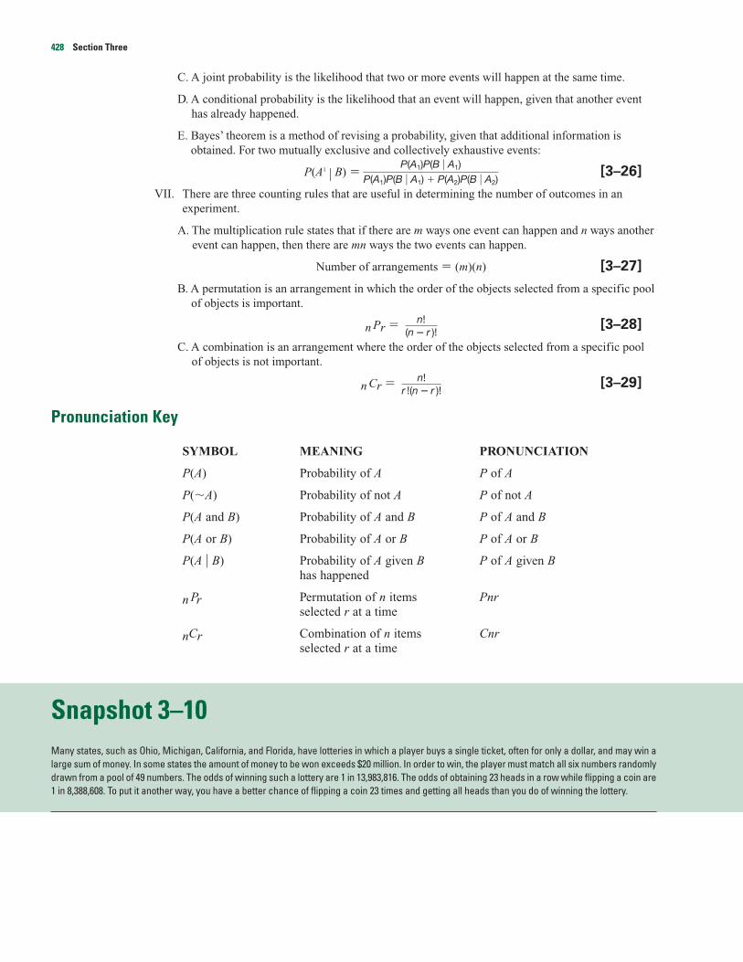
C. A joint probability is the likelihood that two or more events will happen at the same time.
D. A conditional probability is the likelihood that an event will happen, given that another eventhas already happened.
E. Bayes’ theorem is a method of revising a probability, given that additional information isobtained. For two mutually exclusive and collectively exhaustive events:
P(A1 � B) � [3–26]
VII. There are three counting rules that are useful in determining the number of outcomes in anexperiment.
A. The multiplication rule states that if there are m ways one event can happen and n ways anotherevent can happen, then there are mn ways the two events can happen.
Number of arrangements � (m)(n) [3–27]
B. A permutation is an arrangement in which the order of the objects selected from a specific poolof objects is important.
n Pr � [3–28]
C. A combination is an arrangement where the order of the objects selected from a specific poolof objects is not important.
n Cr � [3–29]
Pronunciation Key
SYMBOL MEANING PRONUNCIATION
P(A) Probability of A P of A
P(�A) Probability of not A P of not A
P(A and B) Probability of A and B P of A and B
P(A or B) Probability of A or B P of A or B
P(A � B) Probability of A given B P of A given Bhas happened
n Pr Permutation of n items Pnrselected r at a time
nCr Combination of n items Cnrselected r at a time
Snapshot 3–10Many states, such as Ohio, Michigan, California, and Florida, have lotteries in which a player buys a single ticket, often for only a dollar, and may win alarge sum of money. In some states the amount of money to be won exceeds $20 million. In order to win, the player must match all six numbers randomlydrawn from a pool of 49 numbers. The odds of winning such a lottery are 1 in 13,983,816. The odds of obtaining 23 heads in a row while flipping a coin are1 in 8,388,608. To put it another way, you have a better chance of flipping a coin 23 times and getting all heads than you do of winning the lottery.
n!r !(n � r )!
n!(n � r )!
P(A1)P(B � A1)P(A1)P(B � A1) � P(A2)P(B � A2)
428 Section Three
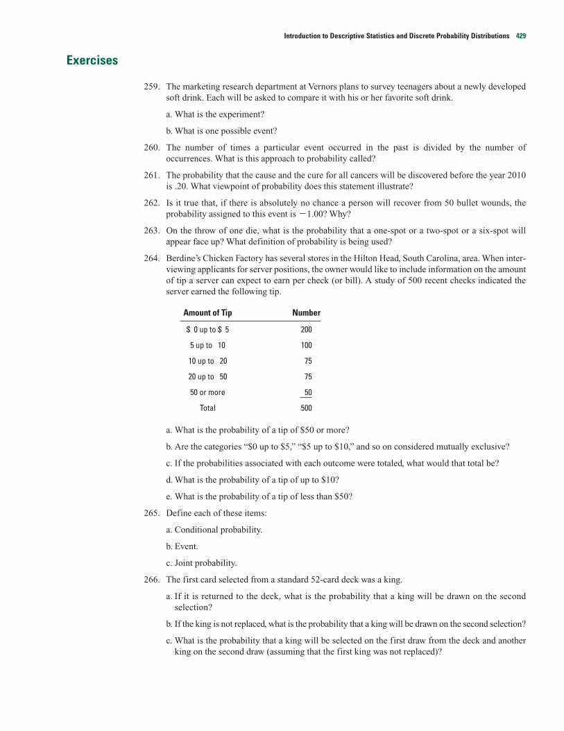
Exercises
259. The marketing research department at Vernors plans to survey teenagers about a newly developedsoft drink. Each will be asked to compare it with his or her favorite soft drink.
a. What is the experiment?
b. What is one possible event?
260. The number of times a particular event occurred in the past is divided by the number ofoccurrences. What is this approach to probability called?
261. The probability that the cause and the cure for all cancers will be discovered before the year 2010is .20. What viewpoint of probability does this statement illustrate?
262. Is it true that, if there is absolutely no chance a person will recover from 50 bullet wounds, theprobability assigned to this event is �1.00? Why?
263. On the throw of one die, what is the probability that a one-spot or a two-spot or a six-spot willappear face up? What definition of probability is being used?
264. Berdine’s Chicken Factory has several stores in the Hilton Head, South Carolina, area. When inter-viewing applicants for server positions, the owner would like to include information on the amountof tip a server can expect to earn per check (or bill). A study of 500 recent checks indicated theserver earned the following tip.
Amount of Tip Number
$ 0 up to $ 5 200
5 up to 10 100
10 up to 20 75
20 up to 50 75
50 or more 50
Total 500
a. What is the probability of a tip of $50 or more?
b. Are the categories “$0 up to $5,” “$5 up to $10,” and so on considered mutually exclusive?
c. If the probabilities associated with each outcome were totaled, what would that total be?
d. What is the probability of a tip of up to $10?
e. What is the probability of a tip of less than $50?
265. Define each of these items:
a. Conditional probability.
b. Event.
c. Joint probability.
266. The first card selected from a standard 52-card deck was a king.
a. If it is returned to the deck, what is the probability that a king will be drawn on the secondselection?
b. If the king is not replaced, what is the probability that a king will be drawn on the second selection?
c. What is the probability that a king will be selected on the first draw from the deck and anotherking on the second draw (assuming that the first king was not replaced)?
Introduction to Descriptive Statistics and Discrete Probability Distributions 429
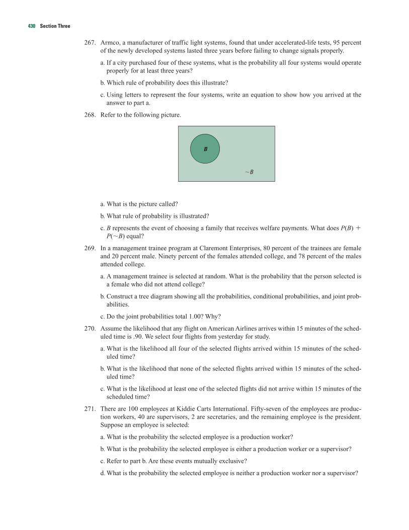
267. Armco, a manufacturer of traffic light systems, found that under accelerated-life tests, 95 percentof the newly developed systems lasted three years before failing to change signals properly.
a. If a city purchased four of these systems, what is the probability all four systems would operateproperly for at least three years?
b. Which rule of probability does this illustrate?
c. Using letters to represent the four systems, write an equation to show how you arrived at theanswer to part a.
268. Refer to the following picture.
a. What is the picture called?
b. What rule of probability is illustrated?
c. B represents the event of choosing a family that receives welfare payments. What does P(B) �P(�B) equal?
269. In a management trainee program at Claremont Enterprises, 80 percent of the trainees are femaleand 20 percent male. Ninety percent of the females attended college, and 78 percent of the malesattended college.
a. A management trainee is selected at random. What is the probability that the person selected isa female who did not attend college?
b. Construct a tree diagram showing all the probabilities, conditional probabilities, and joint prob-abilities.
c. Do the joint probabilities total 1.00? Why?
270. Assume the likelihood that any flight on American Airlines arrives within 15 minutes of the sched-uled time is .90. We select four flights from yesterday for study.
a. What is the likelihood all four of the selected flights arrived within 15 minutes of the sched-uled time?
b. What is the likelihood that none of the selected flights arrived within 15 minutes of the sched-uled time?
c. What is the likelihood at least one of the selected flights did not arrive within 15 minutes of thescheduled time?
271. There are 100 employees at Kiddie Carts International. Fifty-seven of the employees are produc-tion workers, 40 are supervisors, 2 are secretaries, and the remaining employee is the president.Suppose an employee is selected:
a. What is the probability the selected employee is a production worker?
b. What is the probability the selected employee is either a production worker or a supervisor?
c. Refer to part b. Are these events mutually exclusive?
d. What is the probability the selected employee is neither a production worker nor a supervisor?
B
�B
430 Section Three
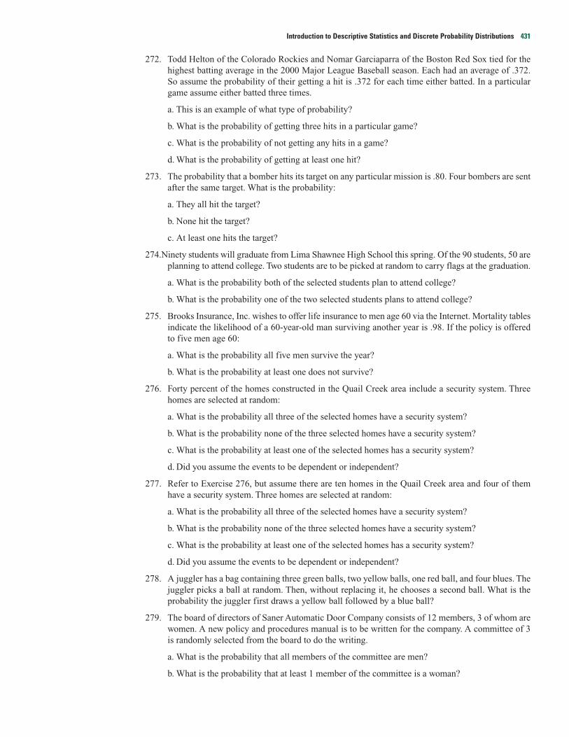
272. Todd Helton of the Colorado Rockies and Nomar Garciaparra of the Boston Red Sox tied for thehighest batting average in the 2000 Major League Baseball season. Each had an average of .372.So assume the probability of their getting a hit is .372 for each time either batted. In a particulargame assume either batted three times.
a. This is an example of what type of probability?
b. What is the probability of getting three hits in a particular game?
c. What is the probability of not getting any hits in a game?
d. What is the probability of getting at least one hit?
273. The probability that a bomber hits its target on any particular mission is .80. Four bombers are sentafter the same target. What is the probability:
a. They all hit the target?
b. None hit the target?
c. At least one hits the target?
274.Ninety students will graduate from Lima Shawnee High School this spring. Of the 90 students, 50 areplanning to attend college. Two students are to be picked at random to carry flags at the graduation.
a. What is the probability both of the selected students plan to attend college?
b. What is the probability one of the two selected students plans to attend college?
275. Brooks Insurance, Inc. wishes to offer life insurance to men age 60 via the Internet. Mortality tablesindicate the likelihood of a 60-year-old man surviving another year is .98. If the policy is offeredto five men age 60:
a. What is the probability all five men survive the year?
b. What is the probability at least one does not survive?
276. Forty percent of the homes constructed in the Quail Creek area include a security system. Threehomes are selected at random:
a. What is the probability all three of the selected homes have a security system?
b. What is the probability none of the three selected homes have a security system?
c. What is the probability at least one of the selected homes has a security system?
d. Did you assume the events to be dependent or independent?
277. Refer to Exercise 276, but assume there are ten homes in the Quail Creek area and four of themhave a security system. Three homes are selected at random:
a. What is the probability all three of the selected homes have a security system?
b. What is the probability none of the three selected homes have a security system?
c. What is the probability at least one of the selected homes has a security system?
d. Did you assume the events to be dependent or independent?
278. A juggler has a bag containing three green balls, two yellow balls, one red ball, and four blues. Thejuggler picks a ball at random. Then, without replacing it, he chooses a second ball. What is theprobability the juggler first draws a yellow ball followed by a blue ball?
279. The board of directors of Saner Automatic Door Company consists of 12 members, 3 of whom arewomen. A new policy and procedures manual is to be written for the company. A committee of 3is randomly selected from the board to do the writing.
a. What is the probability that all members of the committee are men?
b. What is the probability that at least 1 member of the committee is a woman?
Introduction to Descriptive Statistics and Discrete Probability Distributions 431

280. A survey of undergraduate students in the School of Business at Northern University revealed thefollowing regarding the gender and majors of the students:
MajorGender Accounting Management Finance Total
Male 100 150 50 300
Female 100 50 50 200
Total 200 200 100 500
a. What is the probability of selecting a female student?
b. What is the probability of selecting a finance or accounting major?
c. What is the probability of selecting a female or an accounting major? Which rule of addition didyou apply?
d. What is the probability of selecting an accounting major, given that the person selected is a male?
e. Suppose two students are selected randomly to attend a lunch with the president of the univer-sity. What is the probability that both of those selected are accounting majors?
281. The Wood County sheriff classifies crimes by age (in years) of the criminal and whether thecrime is violent or nonviolent. As shown below, a total of 150 crimes were reported by the sher-iff last year.
Age (in years)Type of Crime Under 20 20 to 40 Over 40 Total
Violent 27 41 14 82
NonViolent 12 34 22 68
Total 39 75 36 150
a. What is the probability of selecting a case to analyze and finding it involved a violent crime?
b. What is the probability of selecting a case to analyze and finding the crime was committed bysomeone less than 40 years old?
c. What is the probability of selecting a case that involved a violent crime or an offender less than20 years old? Which rule of addition did you apply?
d. Given that a violent crime is selected for analysis, what is the probability the crime was com-mitted by a person under 20 years old?
e. Two crimes are selected for review by Judge Tybo. What is the probability that both are violentcrimes?
282. Mr. and Mrs. Wilhelms are both retired and living in a retirement community in Arizona. Supposethe probability that a retired man will live another 10 years is .60. The probability that a retiredwoman will live another 10 years is .70.
a. What is the probability that both Mr. and Mrs. Wilhelms will be alive 10 years from now?
b. What is the probability that in 10 years Mr. Wilhelms is not living and Mrs. Wilhelms is living?
c. What is the probability that in 10 years at least one is living?
283. Flashner Marketing Research, Inc. specializes in providing assessments of the prospects forwomen’s apparel shops in shopping malls. Al Flashner, president, reports that he assesses theprospects as good, fair, or poor. Records from previous assessments show that 60 percent of thetime the prospects were rated as good, 30 percent of the time fair, and 10 percent of the time poor.Of those rated good, 80 percent made a profit the first year; of those rated fair, 60 percent made a
432 Section Three

profit the first year; and of those rated poor, 20 percent made a profit the first year. Connie’sApparel was one of Flashner’s clients. Connie’s Apparel made a profit last year. What is the prob-ability that it was given an original rating of poor?
284. There are 400 employees at G. G. Greene Manufacturing Co., and 100 of them smoke. There are250 males working for the company, and 75 of them smoke. What is the probability that anemployee selected at random:
a. Is a male?
b. Smokes?
c. Is male and smokes?
d. Is male or smokes?
285. With each purchase of a large pizza at Tony’s Pizza, the customer receives a coupon that can bescratched to see if a prize will be awarded. The odds of winning a free soft drink are 1 in 10, andthe odds of winning a free large pizza are 1 in 50. You plan to eat lunch tomorrow at Tony’s. Whatis the probability:
a. That you will win either a large pizza or a soft drink?
b. That you will not win a prize?
c. That you will not win a prize on three consecutive visits to Tony’s?
d. That you will win at least one prize on one of your next three visits to Tony’s?
286. For the daily lottery game in Illinois, participants select three numbers between 0 and 9. A numbercannot be selected more than once, so a winning ticket could be, say, 307. Purchasing one ticketallows you to select one set of numbers. The winning numbers are announced on TV each night.
a. How many different outcomes (three-digit numbers) are possible?
b. If you purchase a ticket for the game tonight, what is the likelihood you will win?
c. Suppose you purchase three tickets for tonight’s drawing and select a different number for eachticket. What is the probability that you will not win with any of the tickets?
287. A new job consists of assembling four different parts. All four have different color codes, and theycan be assembled in any order. The production department wants to determine the most efficientway to assemble the four parts. The supervisors are going to conduct some experiments to solve theproblem. First, they plan to assemble the parts in this order — green, black, yellow, and blue — andrecord the time. Then the assembly will be accomplished in a different order. In how many differ-ent ways can the four parts be assembled?
288. It was found that 60 percent of the tourists to China visited the Forbidden City, the Temple ofHeaven, the Great Wall, and other historical sites in or near Beijing. Forty percent visited Xi’anwith its magnificent terracotta soldiers, horses, and chariots, which lay buried for over 2,000 years.Thirty percent of the tourists went to both Beijing and Xi’an. What is the probability that a touristvisited at least one of these places?
289. Two boxes of men’s Old Navy shirts were received from the factory. Box 1 contained 25 mesh poloshirts and 15 Super-T shirts. Box 2 contained 30 mesh polo shirts and 10 Super-T shirts. One of theboxes was selected at random, and a shirt was chosen at random from that box to be inspected. Theshirt was a mesh polo shirt. Given this information, what is the probability that the mesh polo shirtcame from box 1?
290. The operators of Riccardo’s Restaurant want to advertise that they have a large number of differentmeals. They offer 4 soups, 3 salads, 12 entrees, 6 vegetables, and 5 desserts. How many differentmeals do they offer? In addition, Riccardo’s has an “early bird” special: You may omit any part ofthe meal except the entrees for a reduced price. How many different meals do they have for the“early birds”?
Introduction to Descriptive Statistics and Discrete Probability Distributions 433

291. Several years ago Wendy’s Hamburgers advertised that there are 256 different ways to order yourhamburger. You may choose to have, or omit, any combination of the following on your hamburger:mustard, ketchup, onion, pickle, tomato, relish, mayonnaise, and lettuce. Is the advertisement cor-rect? Show how you arrive at your answer.
292. Reynolds Construction Company has agreed not to erect all “look-alike” homes in a new subdivi-sion. Five exterior designs are offered to potential home buyers. The builder has standardized threeinterior plans that can be incorporated in any of the five exteriors. How many different ways canthe exterior and interior plans be offered to potential home buyers?
293. A small rug weaver has decided to use seven compatible colors in her new line of rugs. However,in weaving a rug, only five spindles can be used. In her advertising she wants to indicate the num-ber of different color groupings for sale. How many color groupings using the seven colors takenfive at a time are there? (This assumes that five different colors will go into each rug — i.e., thereare no repetitions of color.)
294. Consideration is being given to forming a Super Ten football conference. The top 10 football teamsin the country, based on past records, would be members of the Super Ten conference. Each teamwould play every other team in the conference during the season. The team winning the most gameswould be declared the national champion. How many games would the conference commissionerhave to schedule each year? (Remember, Oklahoma versus Michigan is the same as Michigan ver-sus Oklahoma.)
295. A new chewing gum has been developed that is helpful to those who want to stop smoking. If 60percent of those people chewing the gum are successful in stopping smoking, what is the proba-bility that in a group of four smokers using the gum at least one quits smoking?
296. The state of Maryland has license plates with three numbers followed by three letters. How manydifferent license plates are possible?
297. A new sports car model has defective brakes 15 percent of the time and a defective steering mech-anism 5 percent of the time. Let’s assume (and hope) that these problems occur independently. Ifone or the other of these problems is present, the car is called a “lemon.” If both of these problemsare present, the car is a “hazard.” Your instructor purchased one of these cars yesterday. What is theprobability it is:
a. A lemon?
b. A hazard?
298. Tim Bleckie is the owner of Bleckie Investment and Real Estate Company. The company recentlypurchased four tracts of land in Holly Farms Estates and six tracts in Newburg Woods. The tractsare all equally desirable and sell for about the same amount.
a. What is the probability that the next two tracts sold will be in Newburg Woods?
b. What is the probability that of the next four sold at least one will be in Holly Farms?
c. Are these events independent or dependent?
299. There are four people being considered for the position of chief executive officer of Dalton Enter-prises. Three of the applicants are over 60 years of age. Two are female, of which only one is over 60.
a. What is the probability that a candidate is over 60 and female?
b. Given that the candidate is male, what is the probability he is less than 60?
c. Given that the person is over 60, what is the probability the person is female?
300. A case of 24 cans contains 1 can that is contaminated. Three cans are to be chosen randomly fortesting.
a. How many different combinations of 3 cans could be selected?
b. What is the probability that the contaminated can is selected for testing?
434 Section Three
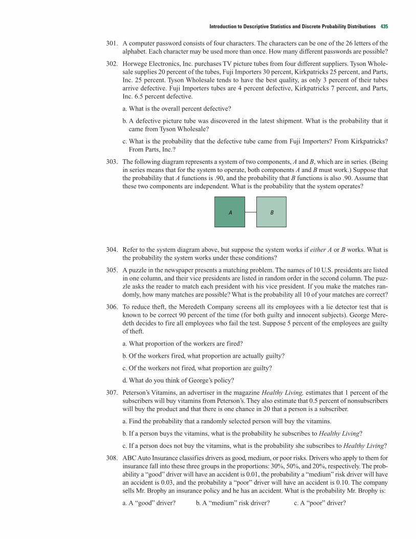
301. A computer password consists of four characters. The characters can be one of the 26 letters of thealphabet. Each character may be used more than once. How many different passwords are possible?
302. Horwege Electronics, Inc. purchases TV picture tubes from four different suppliers. Tyson Whole-sale supplies 20 percent of the tubes, Fuji Importers 30 percent, Kirkpatricks 25 percent, and Parts,Inc. 25 percent. Tyson Wholesale tends to have the best quality, as only 3 percent of their tubesarrive defective. Fuji Importers tubes are 4 percent defective, Kirkpatricks 7 percent, and Parts,Inc. 6.5 percent defective.
a. What is the overall percent defective?
b. A defective picture tube was discovered in the latest shipment. What is the probability that itcame from Tyson Wholesale?
c. What is the probability that the defective tube came from Fuji Importers? From Kirkpatricks?From Parts, Inc.?
303. The following diagram represents a system of two components, A and B, which are in series. (Beingin series means that for the system to operate, both components A and B must work.) Suppose thatthe probability that A functions is .90, and the probability that B functions is also .90. Assume thatthese two components are independent. What is the probability that the system operates?
304. Refer to the system diagram above, but suppose the system works if either A or B works. What isthe probability the system works under these conditions?
305. A puzzle in the newspaper presents a matching problem. The names of 10 U.S. presidents are listedin one column, and their vice presidents are listed in random order in the second column. The puz-zle asks the reader to match each president with his vice president. If you make the matches ran-domly, how many matches are possible? What is the probability all 10 of your matches are correct?
306. To reduce theft, the Meredeth Company screens all its employees with a lie detector test that isknown to be correct 90 percent of the time (for both guilty and innocent subjects). George Mere-deth decides to fire all employees who fail the test. Suppose 5 percent of the employees are guiltyof theft.
a. What proportion of the workers are fired?
b. Of the workers fired, what proportion are actually guilty?
c. Of the workers not fired, what proportion are guilty?
d. What do you think of George’s policy?
307. Peterson’s Vitamins, an advertiser in the magazine Healthy Living, estimates that 1 percent of thesubscribers will buy vitamins from Peterson’s. They also estimate that 0.5 percent of nonsubscriberswill buy the product and that there is one chance in 20 that a person is a subscriber.
a. Find the probability that a randomly selected person will buy the vitamins.
b. If a person buys the vitamins, what is the probability he subscribes to Healthy Living?
c. If a person does not buy the vitamins, what is the probability she subscribes to Healthy Living?
308. ABC Auto Insurance classifies drivers as good, medium, or poor risks. Drivers who apply to them forinsurance fall into these three groups in the proportions: 30%, 50%, and 20%, respectively. The prob-ability a “good” driver will have an accident is 0.01, the probability a “medium” risk driver will havean accident is 0.03, and the probability a “poor” driver will have an accident is 0.10. The companysells Mr. Brophy an insurance policy and he has an accident. What is the probability Mr. Brophy is:
a. A “good” driver? b. A “medium” risk driver? c. A “poor” driver?
A B
Introduction to Descriptive Statistics and Discrete Probability Distributions 435
exercises.com
309. During the 1970s the game show Let’s Make a Deal had a long run on TV. In the show a contestantwas given a choice of three doors, behind one of which was a prize. The other two doors containeda gag gift of some type. After the contestant selected a door, the host of the show then revealed tothem one of the doors from among the two not selected. The host asked the contestant if theywished to switch doors to one of those not chosen. Should the contestant switch? Are the odds ofwinning increased by switching doors?
Go to the following Website, which is administered by the Department of Statistics at theUniversity of South Carolina, and try your strategy: http://www.stat.sc.edu/~west/applets/LetsMakeaDeal.html. Go to the following Website and read about the odds forthe game: http://www.stat.sc.edu/~west/javahtml/LetsMakeaDeal.html. Was yourstrategy correct?
Computer Data Exercises
310. Refer to the Real Estate data (Appendix J), which reports information on homes sold in the Venice,Florida, area during the last year.
a. Sort the data into a table that shows the number of homes that have a pool versus the number thatdon’t have a pool in each of the five townships. If a home is selected at random, compute the fol-lowing probabilities.
(1) The home is in Township 1 or has a pool.
(2) Given that it is in Township 3, that it has a pool.
(3) Has a pool and is in Township 3.
b. Sort the data into a table that shows the number of homes that have a garage versus those thatdon’t have a garage in each of the five townships. If a home is selected at random, compute thefollowing probabilities:
(1) The home has a garage.
(2) Given that it is in Township 5, that it does not have a garage.
(3) The home has a garage and is in Township 3.
(4) Does not have a garage or is in Township 2.
311. Refer to the Baseball 2000 data (Appendix K), which reports information on the 30 Major LeagueBaseball teams for the 2000 season. Set up a variable that divides the teams into two groups, thosethat had a winning season and those that did not. That is, create a variable to count the teams thatwon 81 games or more, and those that won 80 or less. Next create a new variable for attendance,using three categories: attendance less than 1,500,000, attendance of 1,500,000 up to 2,500,000,and attendance of 2,500,000 or more.
a. Create a table that shows the number of teams with a winning season versus those with a losingseason by the three categories of attendance. If a team is selected at random, compute the fol-lowing probabilities:
(1) Having a winning season.
(2) Having a winning season or attendance of more than 2.5 million.
(3) Given attendance of more than 2.5 million, having a winning season.
(4) Having a losing season and drawing less than 1.5 million.
436 Section Three

b. Create a table that shows the number of teams that play on artificial surfaces and natural sur-faces by winning and losing records. If a team is selected at random, compute the followingprobabilities:
(1) Selecting a team with a home field that has a natural surface.
(2) Is the likelihood of selecting a team with a winning record larger for teams withnatural or artificial surfaces?
(3) Having a winning record or playing on an artificial surface.
312. Refer to the Schools data (Appendix M), which refers to 94 school districts in Northwest Ohio.
a. Group the districts based on the percent of students on welfare: “low” (less than 5 percent), “moderate” (between 5 and 10 percent, inclusive), and “high” (more than 10 percent).
(1) A school district is randomly selected. Then a student within that district is chosen.What is the probability the student passed the proficiency exam? Hint: Find themean percent passing and use that value as the probability of passing the exam.
(2) If it is a “low” welfare district, what is the probability the student passed the exam?
(3) What is the probability the student is from a “high” welfare district and passesthe exam?
(4) Find the probability the student is either from a “moderate” welfare district or failedthe exam.
b. Now arrange the districts by size: “small” (less than 1,000 students), “medium” (between 1,000and 3,000 students), or “large” (more than 3,000 students).
(1) What percent of the districts are “small”?
(2) If a district is “small,” estimate the probability it is a “low” welfare district.
(3) What percent of the districts are both “small” and “low” welfare?
(4) What percent are either “small” or “low” welfare?
(5) If three districts are randomly chosen, what is the probability they are all“medium” sized?
Introduction to Descriptive Statistics and Discrete Probability Distributions 437
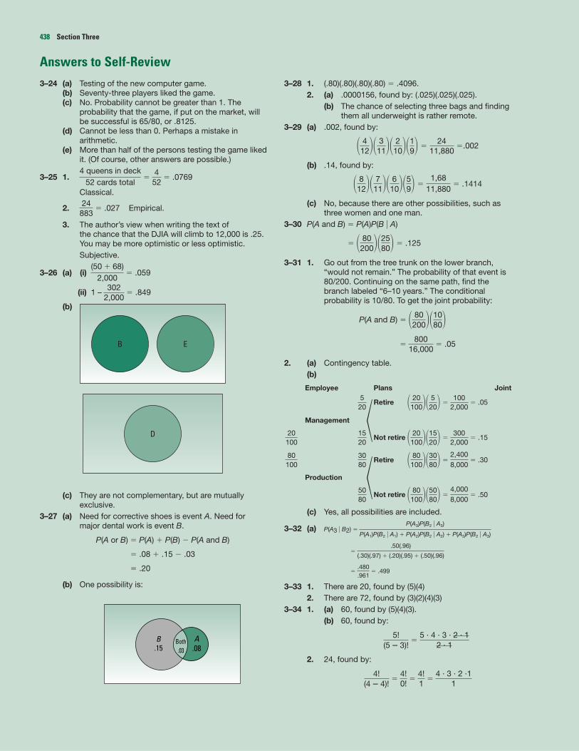
Answers to Self-Review3–24 (a) Testing of the new computer game.
(b) Seventy-three players liked the game.(c) No. Probability cannot be greater than 1. The
probability that the game, if put on the market, willbe successful is 65/80, or .8125.
(d) Cannot be less than 0. Perhaps a mistake inarithmetic.
(e) More than half of the persons testing the game likedit. (Of course, other answers are possible.)
3–25 1. � � .0769
Classical.
2. � .027 Empirical.
3. The author’s view when writing the text ofthe chance that the DJIA will climb to 12,000 is .25.You may be more optimistic or less optimistic.Subjective.
3–26 (a) (i) � .059
(ii) 1 – � .849
(b)
(c) They are not complementary, but are mutuallyexclusive.
3–27 (a) Need for corrective shoes is event A. Need formajor dental work is event B.
P(A or B) � P(A) � P(B) � P(A and B)
� .08 � .15 � .03
� .20
(b) One possibility is:
3–28 1. (.80)(.80)(.80)(.80) � .4096.2. (a) .0000156, found by: (.025)(.025)(.025).
(b) The chance of selecting three bags and findingthem all underweight is rather remote.
3–29 (a) .002, found by:
� �.002
(b) .14, found by:
� � .1414
(c) No, because there are other possibilities, such asthree women and one man.
3–30 P(A and B) � P(A)P(B � A)
� � .125
3–31 1. Go out from the tree trunk on the lower branch,“would not remain.” The probability of that event is80/200. Continuing on the same path, find thebranch labeled “6–10 years.” The conditionalprobability is 10/80. To get the joint probability:
P(A and B) �
� � .05
2. (a) Contingency table.(b)
Employee Plans Joint
Retire � � .05
Management
Not retire � � .15
Retire � � .30
Production
Not retire � � .50
(c) Yes, all possibilities are included.
3–32 (a) P(A3 � B2) �
�
� � .499
3–33 1. There are 20, found by (5)(4)2. There are 72, found by (3)(2)(4)(3)
3–34 1. (a) 60, found by (5)(4)(3).(b) 60, found by:
�
2. 24, found by:
� � �4 · 3 · 2 ·1
14!1
4!0!
4!(4 � 4)!
5 · 4 · 3 · 2 · 12 · 1
5!(5 � 3)!
.480
.961
.50(.96)
(.30)(.97) � (.20)(.95) � (.50)(.96)
P(A3)P(B2 � A3)
P(A1)P(B2 � A1) � P(A2)P(B2 � A2) � P(A3)P(B2 � A3)
4,0008,000� 80
100��5080�
5080
2,4008,000� 80
100��3080�
3080
80100
3002,000� 20
100��1520�
1520
20100
1002,000� 20
100��520�
520
80016,000
� 80200��10
80�
� 80200��25
80�
1,6811,880� 8
12�� 711�� 6
10��59�
2411,880� 4
12�� 311�� 2
10��19�
B.15
A.08
Both.03
D
B E
3022,000
(50 � 68)2,000
24883
452
4 queens in deck52 cards total
438 Section Three

3. 5,040, found by:
�
4. (a) 56 is correct, found by:
8C3 � � � 56
(b) Yes. There are 45 combinations, found by:
10C2 � � � 4510!
2!(10 � 2)!n!
r !(n � r )!
8!3!(8 � 3)!
n!r !(n � r )!
10 · 9 · 8 · 7 · 6 · 5 · 4 · 3 · 2 · 16 · 5 · 4 · 3 · 2 · 1
10!(10 � 4)!
Introduction to Descriptive Statistics and Discrete Probability Distributions 439