Section 4.1: Introduction to Rational Functions, from College … … · · 2017-11-01Chapter 4....

Section 4.1: Introduction to Rational Functions, from College Algebra: Corrected Edition by Carl Stitz, Ph.D. and Jeff Zeager, Ph.D. is available under a Creative Commons Attribution-NonCommercial-ShareAlike 3.0 license. © 2013, Carl Stitz.

http://www.stitz-zeager.com/szca07042013.pdf

http://www.stitz-zeager.com/szca07042013.pdf

http://creativecommons.org/licenses/by-nc-sa/3.0/deed.en_US

http://creativecommons.org/licenses/by-nc-sa/3.0/deed.en_US

Chapter 4

Rational Functions

4.1 Introduction to Rational Functions

If we add, subtract or multiply polynomial functions according to the function arithmetic rulesdefined in Section 1.5, we will produce another polynomial function. If, on the other hand, wedivide two polynomial functions, the result may not be a polynomial. In this chapter we studyrational functions - functions which are ratios of polynomials.

Definition 4.1. A rational function is a function which is the ratio of polynomial functions.Said differently, r is a rational function if it is of the form

r(x) =p(x)

q(x),

where p and q are polynomial functions.a

aAccording to this definition, all polynomial functions are also rational functions. (Take q(x) = 1).

As we recall from Section 1.4, we have domain issues anytime the denominator of a fraction iszero. In the example below, we review this concept as well as some of the arithmetic of rationalexpressions.

Example 4.1.1. Find the domain of the following rational functions. Write them in the form p(x)q(x)

for polynomial functions p and q and simplify.

1. f(x) =2x− 1

x+ 12. g(x) = 2− 3

x+ 1

3. h(x) =2x2 − 1

x2 − 1− 3x− 2

x2 − 14. r(x) =

2x2 − 1

x2 − 1÷ 3x− 2

x2 − 1

Solution.

1. To find the domain of f , we proceed as we did in Section 1.4: we find the zeros of thedenominator and exclude them from the domain. Setting x+1 = 0 results in x = −1. Hence,

302 Rational Functions

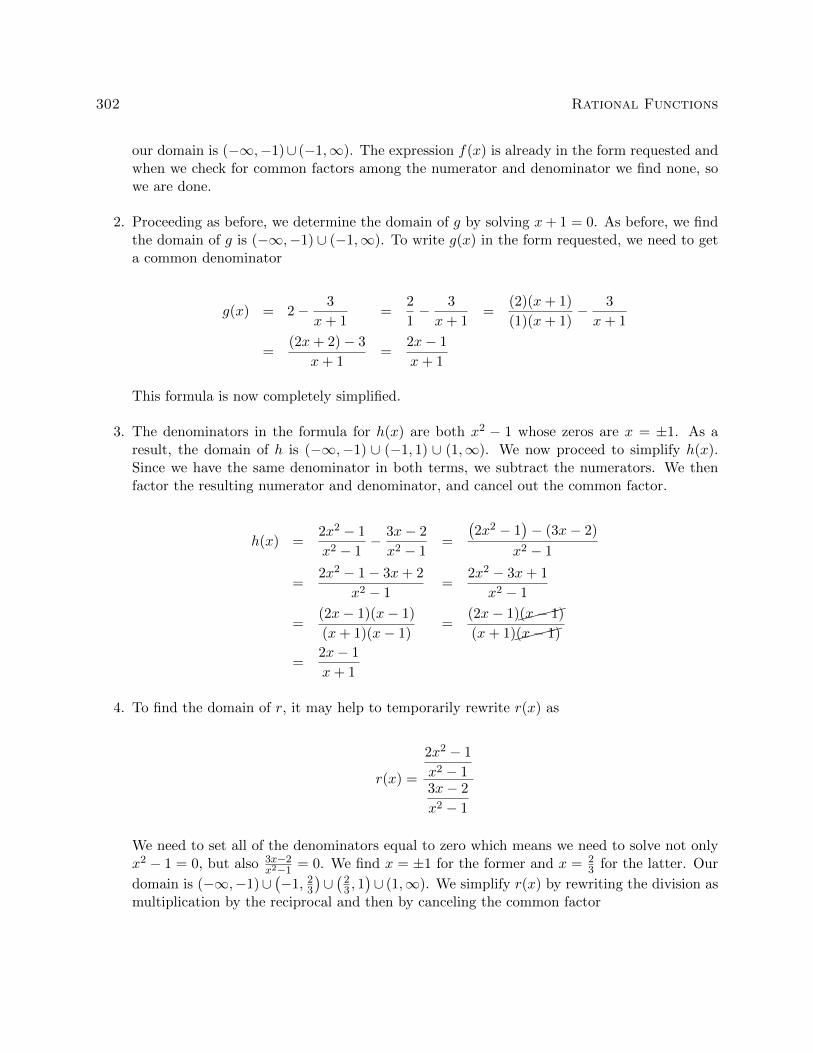
our domain is (−∞,−1)∪ (−1,∞). The expression f(x) is already in the form requested andwhen we check for common factors among the numerator and denominator we find none, sowe are done.

2. Proceeding as before, we determine the domain of g by solving x+ 1 = 0. As before, we findthe domain of g is (−∞,−1) ∪ (−1,∞). To write g(x) in the form requested, we need to geta common denominator

g(x) = 2− 3

x+ 1=

2

1− 3

x+ 1=

(2)(x+ 1)

(1)(x+ 1)− 3

x+ 1

=(2x+ 2)− 3

x+ 1=

2x− 1

x+ 1

This formula is now completely simplified.

3. The denominators in the formula for h(x) are both x2 − 1 whose zeros are x = ±1. As aresult, the domain of h is (−∞,−1) ∪ (−1, 1) ∪ (1,∞). We now proceed to simplify h(x).Since we have the same denominator in both terms, we subtract the numerators. We thenfactor the resulting numerator and denominator, and cancel out the common factor.

h(x) =2x2 − 1

x2 − 1− 3x− 2

x2 − 1=

(2x2 − 1

)− (3x− 2)

x2 − 1

=2x2 − 1− 3x+ 2

x2 − 1=

2x2 − 3x+ 1

x2 − 1

=(2x− 1)(x− 1)

(x+ 1)(x− 1)=

(2x− 1)(x− 1)

(x+ 1)(x− 1)

=2x− 1

x+ 1

4. To find the domain of r, it may help to temporarily rewrite r(x) as

r(x) =

2x2 − 1

x2 − 13x− 2

x2 − 1

We need to set all of the denominators equal to zero which means we need to solve not onlyx2 − 1 = 0, but also 3x−2

x2−1= 0. We find x = ±1 for the former and x = 2

3 for the latter. Our

domain is (−∞,−1)∪(−1, 2

3

)∪(

23 , 1)∪ (1,∞). We simplify r(x) by rewriting the division as

multiplication by the reciprocal and then by canceling the common factor

4.1 Introduction to Rational Functions 303

r(x) =2x2 − 1

x2 − 1÷ 3x− 2

x2 − 1=

2x2 − 1

x2 − 1· x

2 − 1

3x− 2=

(2x2 − 1

) (x2 − 1

)(x2 − 1) (3x− 2)

=

(2x2 − 1

)

(x2 − 1

)

(x2 − 1

)(3x− 2)

=2x2 − 1

3x− 2

A few remarks about Example 4.1.1 are in order. Note that the expressions for f(x), g(x) andh(x) work out to be the same. However, only two of these functions are actually equal. Recall thatfunctions are ultimately sets of ordered pairs,1 so for two functions to be equal, they need, amongother things, to have the same domain. Since f(x) = g(x) and f and g have the same domain, theyare equal functions. Even though the formula h(x) is the same as f(x), the domain of h is differentthan the domain of f , and thus they are different functions.

We now turn our attention to the graphs of rational functions. Consider the function f(x) = 2x−1x+1

from Example 4.1.1. Using a graphing calculator, we obtain

Two behaviors of the graph are worthy of further discussion. First, note that the graph appearsto ‘break’ at x = −1. We know from our last example that x = −1 is not in the domain of fwhich means f(−1) is undefined. When we make a table of values to study the behavior of f nearx = −1 we see that we can get ‘near’ x = −1 from two directions. We can choose values a littleless than −1, for example x = −1.1, x = −1.01, x = −1.001, and so on. These values are said to‘approach −1 from the left.’ Similarly, the values x = −0.9, x = −0.99, x = −0.999, etc., are saidto ‘approach −1 from the right.’ If we make two tables, we find that the numerical results confirmwhat we see graphically.

x f(x) (x, f(x))

−1.1 32 (−1.1, 32)

−1.01 302 (−1.01, 302)

−1.001 3002 (−1.001, 3002)

−1.0001 30002 (−1.001, 30002)

x f(x) (x, f(x))

−0.9 −28 (−0.9,−28)

−0.99 −298 (−0.99,−298)

−0.999 −2998 (−0.999,−2998)

−0.9999 −29998 (−0.9999,−29998)

As the x values approach −1 from the left, the function values become larger and larger positivenumbers.2 We express this symbolically by stating as x → −1−, f(x) → ∞. Similarly, usinganalogous notation, we conclude from the table that as x → −1+, f(x) → −∞. For this type of

1You should review Sections 1.2 and 1.3 if this statement caught you off guard.2We would need Calculus to confirm this analytically.


unbounded behavior, we say the graph of y = f(x) has a vertical asymptote of x = −1. Roughlyspeaking, this means that near x = −1, the graph looks very much like the vertical line x = −1.

The other feature worthy of note about the graph of y = f(x) is that it seems to ‘level off’ on theleft and right hand sides of the screen. This is a statement about the end behavior of the function.As we discussed in Section 3.1, the end behavior of a function is its behavior as x attains larger3 andlarger negative values without bound, x → −∞, and as x becomes large without bound, x → ∞.Making tables of values, we find

x f(x) (x, f(x))

−10 ≈ 2.3333 ≈ (−10, 2.3333)

−100 ≈ 2.0303 ≈ (−100, 2.0303)

−1000 ≈ 2.0030 ≈ (−1000, 2.0030)

−10000 ≈ 2.0003 ≈ (−10000, 2.0003)

x f(x) (x, f(x))

10 ≈ 1.7273 ≈ (10, 1.7273)

100 ≈ 1.9703 ≈ (100, 1.9703)

1000 ≈ 1.9970 ≈ (1000, 1.9970)

10000 ≈ 1.9997 ≈ (10000, 1.9997)

From the tables, we see that as x → −∞, f(x) → 2+ and as x → ∞, f(x) → 2−. Here the ‘+’means ‘from above’ and the ‘−’ means ‘from below’. In this case, we say the graph of y = f(x) hasa horizontal asymptote of y = 2. This means that the end behavior of f resembles the horizontalline y = 2, which explains the ‘leveling off’ behavior we see in the calculator’s graph. We formalizethe concepts of vertical and horizontal asymptotes in the following definitions.

Definition 4.2. The line x = c is called a vertical asymptote of the graph of a functiony = f(x) if as x→ c− or as x→ c+, either f(x)→∞ or f(x)→ −∞.

Definition 4.3. The line y = c is called a horizontal asymptote of the graph of a functiony = f(x) if as x→ −∞ or as x→∞, f(x)→ c.

Note that in Definition 4.3, we write f(x) → c (not f(x) → c+ or f(x) → c−) because we areunconcerned from which direction the values f(x) approach the value c, just as long as they do so.4

In our discussion following Example 4.1.1, we determined that, despite the fact that the formula forh(x) reduced to the same formula as f(x), the functions f and h are different, since x = 1 is in the

domain of f , but x = 1 is not in the domain of h. If we graph h(x) = 2x2−1x2−1

− 3x−2x2−1

using a graphingcalculator, we are surprised to find that the graph looks identical to the graph of y = f(x). Thereis a vertical asymptote at x = −1, but near x = 1, everything seem fine. Tables of values providenumerical evidence which supports the graphical observation.

3Here, the word ‘larger’ means larger in absolute value.4As we shall see in the next section, the graphs of rational functions may, in fact, cross their horizontal asymptotes.

If this happens, however, it does so only a finite number of times, and so for each choice of x → −∞ and x → ∞,f(x) will approach c from either below (in the case f(x)→ c−) or above (in the case f(x)→ c+.) We leave f(x)→ cgeneric in our definition, however, to allow this concept to apply to less tame specimens in the Precalculus zoo, suchas Exercise 50 in Section 10.5.


x h(x) (x, h(x))

0.9 ≈ 0.4210 ≈ (0.9, 0.4210)

0.99 ≈ 0.4925 ≈ (0.99, 0.4925)

0.999 ≈ 0.4992 ≈ (0.999, 0.4992)

0.9999 ≈ 0.4999 ≈ (0.9999, 0.4999)

x h(x) (x, h(x))

1.1 ≈ 0.5714 ≈ (1.1, 0.5714)

1.01 ≈ 0.5075 ≈ (1.01, 0.5075)

1.001 ≈ 0.5007 ≈ (1.001, 0.5007)

1.0001 ≈ 0.5001 ≈ (1.0001, 0.5001)

We see that as x → 1−, h(x) → 0.5− and as x → 1+, h(x) → 0.5+. In other words, the points onthe graph of y = h(x) are approaching (1, 0.5), but since x = 1 is not in the domain of h, it wouldbe inaccurate to fill in a point at (1, 0.5). As we’ve done in past sections when something like thisoccurs,5 we put an open circle (also called a hole in this case6) at (1, 0.5). Below is a detailedgraph of y = h(x), with the vertical and horizontal asymptotes as dashed lines.

x

y

−4 −3 −2 1 2 3 4−1

−2

−3

−4

−5

−6

1

3

4

5

6

7

8

Neither x = −1 nor x = 1 are in the domain of h, yet the behavior of the graph of y = h(x) isdrastically different near these x-values. The reason for this lies in the second to last step whenwe simplified the formula for h(x) in Example 4.1.1, where we had h(x) = (2x−1)(x−1)

(x+1)(x−1) . The reason

x = −1 is not in the domain of h is because the factor (x + 1) appears in the denominator ofh(x); similarly, x = 1 is not in the domain of h because of the factor (x − 1) in the denominatorof h(x). The major difference between these two factors is that (x − 1) cancels with a factor inthe numerator whereas (x + 1) does not. Loosely speaking, the trouble caused by (x − 1) in thedenominator is canceled away while the factor (x + 1) remains to cause mischief. This is why thegraph of y = h(x) has a vertical asymptote at x = −1 but only a hole at x = 1. These observationsare generalized and summarized in the theorem below, whose proof is found in Calculus.

5For instance, graphing piecewise defined functions in Section 1.6.6In Calculus, we will see how these ‘holes’ can be ‘plugged’ when embarking on a more advanced study of continuity.


Theorem 4.1. Location of Vertical Asymptotes and Holes:a Suppose r is a rationalfunction which can be written as r(x) = p(x)

q(x) where p and q have no common zeros.b Let c be areal number which is not in the domain of r.

If q(c) 6= 0, then the graph of y = r(x) has a hole at(c, p(c)q(c)

).

If q(c) = 0, then the line x = c is a vertical asymptote of the graph of y = r(x).

aOr, ‘How to tell your asymptote from a hole in the graph.’bIn other words, r(x) is in lowest terms.

In English, Theorem 4.1 says that if x = c is not in the domain of r but, when we simplify r(x), itno longer makes the denominator 0, then we have a hole at x = c. Otherwise, the line x = c is avertical asymptote of the graph of y = r(x).

Example 4.1.2. Find the vertical asymptotes of, and/or holes in, the graphs of the followingrational functions. Verify your answers using a graphing calculator, and describe the behavior ofthe graph near them using proper notation.

1. f(x) =2x

x2 − 3 2. g(x) =x2 − x− 6

x2 − 9

3. h(x) =x2 − x− 6

x2 + 94. r(x) =

x2 − x− 6

x2 + 4x+ 4

Solution.

1. To use Theorem 4.1, we first find all of the real numbers which aren’t in the domain of f . Todo so, we solve x2 − 3 = 0 and get x = ±

√3. Since the expression f(x) is in lowest terms,

there is no cancellation possible, and we conclude that the lines x = −√

3 and x =√

3 arevertical asymptotes to the graph of y = f(x). The calculator verifies this claim, and from the

graph, we see that as x → −√

3−

, f(x) → −∞, as x → −√

3+

, f(x) → ∞, as x →√

3−

,

f(x)→ −∞, and finally as x→√

3+

, f(x)→∞.

2. Solving x2 − 9 = 0 gives x = ±3. In lowest terms g(x) = x2−x−6x2−9

= (x−3)(x+2)(x−3)(x+3) = x+2

x+3 . Sincex = −3 continues to make trouble in the denominator, we know the line x = −3 is a verticalasymptote of the graph of y = g(x). Since x = 3 no longer produces a 0 in the denominator,we have a hole at x = 3. To find the y-coordinate of the hole, we substitute x = 3 into x+2

x+3

and find the hole is at(3, 5

6

). When we graph y = g(x) using a calculator, we clearly see the

vertical asymptote at x = −3, but everything seems calm near x = 3. Hence, as x → −3−,g(x)→∞, as x→ −3+, g(x)→ −∞, as x→ 3−, g(x)→ 5

6

−, and as x→ 3+, g(x)→ 5

6

+.


The graph of y = f(x) The graph of y = g(x)

3. The domain of h is all real numbers, since x2 + 9 = 0 has no real solutions. Accordingly, thegraph of y = h(x) is devoid of both vertical asymptotes and holes.

4. Setting x2 + 4x + 4 = 0 gives us x = −2 as the only real number of concern. Simplifying,we see r(x) = x2−x−6

x2+4x+4= (x−3)(x+2)

(x+2)2 = x−3x+2 . Since x = −2 continues to produce a 0 in the

denominator of the reduced function, we know x = −2 is a vertical asymptote to the graph.The calculator bears this out, and, moreover, we see that as x → −2−, r(x) → ∞ and asx→ −2+, r(x)→ −∞.

The graph of y = h(x) The graph of y = r(x)

Our next example gives us a physical interpretation of a vertical asymptote. This type of modelarises from a family of equations cheerily named ‘doomsday’ equations.7

Example 4.1.3. A mathematical model for the population P , in thousands, of a certain speciesof bacteria, t days after it is introduced to an environment is given by P (t) = 100

(5−t)2 , 0 ≤ t < 5.

1. Find and interpret P (0).

2. When will the population reach 100,000?

3. Determine the behavior of P as t → 5−. Interpret this result graphically and within thecontext of the problem.

7These functions arise in Differential Equations. The unfortunate name will make sense shortly.


Solution.

1. Substituting t = 0 gives P (0) = 100(5−0)2 = 4, which means 4000 bacteria are initially introduced

into the environment.

2. To find when the population reaches 100,000, we first need to remember that P (t) is measuredin thousands. In other words, 100,000 bacteria corresponds to P (t) = 100. Substituting forP (t) gives the equation 100

(5−t)2 = 100. Clearing denominators and dividing by 100 gives

(5 − t)2 = 1, which, after extracting square roots, produces t = 4 or t = 6. Of these twosolutions, only t = 4 in our domain, so this is the solution we keep. Hence, it takes 4 days forthe population of bacteria to reach 100,000.

3. To determine the behavior of P as t→ 5−, we can make a table

t P (t)

4.9 10000

4.99 1000000

4.999 100000000

4.9999 10000000000

In other words, as t → 5−, P (t) → ∞. Graphically, the line t = 5 is a vertical asymptote ofthe graph of y = P (t). Physically, this means that the population of bacteria is increasingwithout bound as we near 5 days, which cannot actually happen. For this reason, t = 5 iscalled the ‘doomsday’ for this population. There is no way any environment can supportinfinitely many bacteria, so shortly before t = 5 the environment would collapse.

Now that we have thoroughly investigated vertical asymptotes, we can turn our attention to hori-zontal asymptotes. The next theorem tells us when to expect horizontal asymptotes.

Theorem 4.2. Location of Horizontal Asymptotes: Suppose r is a rational function andr(x) = p(x)

q(x) , where p and q are polynomial functions with leading coefficients a and b, respectively.

If the degree of p(x) is the same as the degree of q(x), then y = ab is thea horizontal

asymptote of the graph of y = r(x).

If the degree of p(x) is less than the degree of q(x), then y = 0 is the horizontal asymptoteof the graph of y = r(x).

If the degree of p(x) is greater than the degree of q(x), then the graph of y = r(x) has nohorizontal asymptotes.

aThe use of the definite article will be justified momentarily.

Like Theorem 4.1, Theorem 4.2 is proved using Calculus. Nevertheless, we can understand the ideabehind it using our example f(x) = 2x−1

x+1 . If we interpret f(x) as a division problem, (2x−1)÷(x+1),


we find that the quotient is 2 with a remainder of −3. Using what we know about polynomialdivision, specifically Theorem 3.4, we get 2x − 1 = 2(x + 1) − 3. Dividing both sides by (x + 1)gives 2x−1

x+1 = 2 − 3x+1 . (You may remember this as the formula for g(x) in Example 4.1.1.) As x

becomes unbounded in either direction, the quantity 3x+1 gets closer and closer to 0 so that the

values of f(x) become closer and closer8 to 2. In symbols, as x→ ±∞, f(x)→ 2, and we have theresult.9 Notice that the graph gets close to the same y value as x → −∞ or x → ∞. This meansthat the graph can have only one horizontal asymptote if it is going to have one at all. Thus wewere justified in using ‘the’ in the previous theorem.

Alternatively, we can use what we know about end behavior of polynomials to help us understandthis theorem. From Theorem 3.2, we know the end behavior of a polynomial is determined by itsleading term. Applying this to the numerator and denominator of f(x), we get that as x → ±∞,f(x) = 2x−1

x+1 ≈2xx = 2. This last approach is useful in Calculus, and, indeed, is made rigorous there.

(Keep this in mind for the remainder of this paragraph.) Applying this reasoning to the general

case, suppose r(x) = p(x)q(x) where a is the leading coefficient of p(x) and b is the leading coefficient

of q(x). As x → ±∞, r(x) ≈ axn

bxm , where n and m are the degrees of p(x) and q(x), respectively.If the degree of p(x) and the degree of q(x) are the same, then n = m so that r(x) ≈ a

b , whichmeans y = a

b is the horizontal asymptote in this case. If the degree of p(x) is less than the degreeof q(x), then n < m, so m− n is a positive number, and hence, r(x) ≈ a

bxm−n → 0 as x→ ±∞. Ifthe degree of p(x) is greater than the degree of q(x), then n > m, and hence n −m is a positive

number and r(x) ≈ axn−m

b , which becomes unbounded as x→ ±∞. As we said before, if a rationalfunction has a horizontal asymptote, then it will have only one. (This is not true for other typesof functions we shall see in later chapters.)

Example 4.1.4. List the horizontal asymptotes, if any, of the graphs of the following functions.Verify your answers using a graphing calculator, and describe the behavior of the graph near themusing proper notation.

1. f(x) =5x

x2 + 1 2. g(x) =x2 − 4

x+ 13. h(x) =

6x3 − 3x+ 1

5− 2x3

Solution.

1. The numerator of f(x) is 5x, which has degree 1. The denominator of f(x) is x2 + 1, whichhas degree 2. Applying Theorem 4.2, y = 0 is the horizontal asymptote. Sure enough, we seefrom the graph that as x→ −∞, f(x)→ 0− and as x→∞, f(x)→ 0+.

2. The numerator of g(x), x2 − 4, has degree 2, but the degree of the denominator, x + 1, hasdegree 1. By Theorem 4.2, there is no horizontal asymptote. From the graph, we see thatthe graph of y = g(x) doesn’t appear to level off to a constant value, so there is no horizontalasymptote.10

8As seen in the tables immediately preceding Definition 4.2.9More specifically, as x→ −∞, f(x)→ 2+, and as x→∞, f(x)→ 2−.

10Sit tight! We’ll revisit this function and its end behavior shortly.


3. The degrees of the numerator and denominator of h(x) are both three, so Theorem 4.2 tellsus y = 6

−2 = −3 is the horizontal asymptote. We see from the calculator’s graph that asx→ −∞, h(x)→ −3+, and as x→∞, h(x)→ −3−.

The graph of y = f(x) The graph of y = g(x) The graph of y = h(x)

Our next example of the section gives us a real-world application of a horizontal asymptote.11

Example 4.1.5. The number of students N at local college who have had the flu t months afterthe semester begins can be modeled by the formula N(t) = 500− 450

1+3t for t ≥ 0.

1. Find and interpret N(0).

2. How long will it take until 300 students will have had the flu?

3. Determine the behavior of N as t → ∞. Interpret this result graphically and within thecontext of the problem.

Solution.

1. N(0) = 500 − 4501+3(0) = 50. This means that at the beginning of the semester, 50 students

have had the flu.

2. We set N(t) = 300 to get 500− 4501+3t = 300 and solve. Isolating the fraction gives 450

1+3t = 200.

Clearing denominators gives 450 = 200(1 + 3t). Finally, we get t = 512 . This means it will

take 512 months, or about 13 days, for 300 students to have had the flu.

3. To determine the behavior of N as t→∞, we can use a table.

t N(t)

10 ≈ 485.48

100 ≈ 498.50

1000 ≈ 499.85

10000 ≈ 499.98

The table suggests that as t → ∞, N(t) → 500. (More specifically, 500−.) This means astime goes by, only a total of 500 students will have ever had the flu.

11Though the population below is more accurately modeled with the functions in Chapter 6, we approximate it(using Calculus, of course!) using a rational function.


We close this section with a discussion of the third (and final!) kind of asymptote which can be

associated with the graphs of rational functions. Let us return to the function g(x) = x2−4x+1 in

Example 4.1.4. Performing long division,12 we get g(x) = x2−4x+1 = x − 1 − 3

x+1 . Since the term3

x+1 → 0 as x → ±∞, it stands to reason that as x becomes unbounded, the function values

g(x) = x− 1− 3x+1 ≈ x− 1. Geometrically, this means that the graph of y = g(x) should resemble

the line y = x− 1 as x→ ±∞. We see this play out both numerically and graphically below.

x g(x) x− 1

−10 ≈ −10.6667 −11

−100 ≈ −100.9697 −101

−1000 ≈ −1000.9970 −1001

−10000 ≈ −10000.9997 −10001

x g(x) x− 1

10 ≈ 8.7273 9

100 ≈ 98.9703 99

1000 ≈ 998.9970 999

10000 ≈ 9998.9997 9999

y = g(x) and y = x− 1 y = g(x) and y = x− 1as x→ −∞ as x→∞

The way we symbolize the relationship between the end behavior of y = g(x) with that of the liney = x − 1 is to write ‘as x → ±∞, g(x) → x − 1.’ In this case, we say the line y = x − 1 is aslant asymptote13 to the graph of y = g(x). Informally, the graph of a rational function has aslant asymptote if, as x → ∞ or as x → −∞, the graph resembles a non-horizontal, or ‘slanted’line. Formally, we define a slant asymptote as follows.

Definition 4.4. The line y = mx + b where m 6= 0 is called a slant asymptote of the graphof a function y = f(x) if as x→ −∞ or as x→∞, f(x)→ mx+ b.

A few remarks are in order. First, note that the stipulation m 6= 0 in Definition 4.4 is whatmakes the ‘slant’ asymptote ‘slanted’ as opposed to the case when m = 0 in which case we’d have ahorizontal asymptote. Secondly, while we have motivated what me mean intuitively by the notation‘f(x)→ mx+b,’ like so many ideas in this section, the formal definition requires Calculus. Anotherway to express this sentiment, however, is to rephrase ‘f(x) → mx + b’ as ‘f(x)− (mx + b) → 0.’In other words, the graph of y = f(x) has the slant asymptote y = mx+ b if and only if the graphof y = f(x)− (mx+ b) has a horizontal asymptote y = 0.

12See the remarks following Theorem 4.2.13Also called an ‘oblique’ asymptote in some, ostensibly higher class (and more expensive), texts.


Our next task is to determine the conditions under which the graph of a rational function hasa slant asymptote, and if it does, how to find it. In the case of g(x) = x2−4

x+1 , the degree of the

numerator x2 − 4 is 2, which is exactly one more than the degree if its denominator x + 1 whichis 1. This results in a linear quotient polynomial, and it is this quotient polynomial which is theslant asymptote. Generalizing this situation gives us the following theorem.14

Theorem 4.3. Determination of Slant Asymptotes: Suppose r is a rational function andr(x) = p(x)

q(x) , where the degree of p is exactly one more than the degree of q. Then the graph of

y = r(x) has the slant asymptote y = L(x) where L(x) is the quotient obtained by dividingp(x) by q(x).

In the same way that Theorem 4.2 gives us an easy way to see if the graph of a rational functionr(x) = p(x)

q(x) has a horizontal asymptote by comparing the degrees of the numerator and denominator,Theorem 4.3 gives us an easy way to check for slant asymptotes. Unlike Theorem 4.2, which givesus a quick way to find the horizontal asymptotes (if any exist), Theorem 4.3 gives us no such‘short-cut’. If a slant asymptote exists, we have no recourse but to use long division to find it.15

Example 4.1.6. Find the slant asymptotes of the graphs of the following functions if they exist.Verify your answers using a graphing calculator and describe the behavior of the graph near themusing proper notation.

1. f(x) =x2 − 4x+ 2

1− x2. g(x) =

x2 − 4

x− 23. h(x) =

x3 + 1

x2 − 4

Solution.

1. The degree of the numerator is 2 and the degree of the denominator is 1, so Theorem 4.3guarantees us a slant asymptote. To find it, we divide 1 − x = −x + 1 into x2 − 4x + 2 andget a quotient of −x+ 3, so our slant asymptote is y = −x+ 3. We confirm this graphically,and we see that as x → −∞, the graph of y = f(x) approaches the asymptote from below,and as x→∞, the graph of y = f(x) approaches the asymptote from above.16

2. As with the previous example, the degree of the numerator g(x) = x2−4x−2 is 2 and the degree

of the denominator is 1, so Theorem 4.3 applies. In this case,

g(x) =x2 − 4

x− 2=

(x+ 2)(x− 2)

(x− 2)=

(x+ 2)(x− 2)

: 1

(x− 2)= x+ 2, x 6= 2

14Once again, this theorem is brought to you courtesy of Theorem 3.4 and Calculus.15That’s OK, though. In the next section, we’ll use long division to analyze end behavior and it’s worth the effort!16Note that we are purposefully avoiding notation like ‘as x→∞, f(x)→ (−x+ 3)+. While it is possible to define

these notions formally with Calculus, it is not standard to do so. Besides, with the introduction of the symbol ‘’ inthe next section, the authors feel we are in enough trouble already.


so we have that the slant asymptote y = x+ 2 is identical to the graph of y = g(x) except atx = 2 (where the latter has a ‘hole’ at (2, 4).) The calculator supports this claim.17

3. For h(x) = x3+1x2−4

, the degree of the numerator is 3 and the degree of the denominator is 2 so

again, we are guaranteed the existence of a slant asymptote. The long division(x3 + 1

)÷(

x2 − 4)

gives a quotient of just x, so our slant asymptote is the line y = x. The calculatorconfirms this, and we find that as x→ −∞, the graph of y = h(x) approaches the asymptotefrom below, and as x→∞, the graph of y = h(x) approaches the asymptote from above.

The graph of y = f(x) The graph of y = g(x) The graph of y = h(x)

The reader may be a bit disappointed with the authors at this point owing to the fact that in Exam-ples 4.1.2, 4.1.4, and 4.1.6, we used the calculator to determine function behavior near asymptotes.We rectify that in the next section where we, in excruciating detail, demonstrate the usefulness of‘number sense’ to reveal this behavior analytically.

17While the word ‘asymptote’ has the connotation of ‘approaching but not equaling,’ Definitions 4.3 and 4.4 invitethe same kind of pathologies we saw with Definitions 1.11 in Section 1.6.


4.1.1 Exercises

In Exercises 1 - 18, for the given rational function f :

Find the domain of f .

Identify any vertical asymptotes of the graph of y = f(x).

Identify any holes in the graph.

Find the horizontal asymptote, if it exists.

Find the slant asymptote, if it exists.

Graph the function using a graphing utility and describe the behavior near the asymptotes.

1. f(x) =x

3x− 6 2. f(x) =3 + 7x

5− 2x3. f(x) =

x

x2 + x− 12

4. f(x) =x

x2 + 1 5. f(x) =x+ 7

(x+ 3)2 6. f(x) =x3 + 1

x2 − 1

7. f(x) =4x

x2 + 48. f(x) =

4x

x2 − 4 9. f(x) =x2 − x− 12

x2 + x− 6

10. f(x) =3x2 − 5x− 2

x2 − 911. f(x) =

x3 + 2x2 + x

x2 − x− 212. f(x) =

x3 − 3x+ 1

x2 + 1

13. f(x) =2x2 + 5x− 3

3x+ 214. f(x) =

−x3 + 4x

x2 − 915. f(x) =

−5x4 − 3x3 + x2 − 10

x3 − 3x2 + 3x− 1

16. f(x) =x3

1− x17. f(x) =

18− 2x2

x2 − 918. f(x) =

x3 − 4x2 − 4x− 5

x2 + x+ 1

19. The cost C in dollars to remove p% of the invasive species of Ippizuti fish from SasquatchPond is given by

C(p) =1770p

100− p, 0 ≤ p < 100

(a) Find and interpret C(25) and C(95).

(b) What does the vertical asymptote at x = 100 mean within the context of the problem?

(c) What percentage of the Ippizuti fish can you remove for $40000?

20. In Exercise 71 in Section 1.4, the population of Sasquatch in Portage County was modeledby the function

P (t) =150t

t+ 15,

where t = 0 represents the year 1803. Find the horizontal asymptote of the graph of y = P (t)and explain what it means.


21. Recall from Example 1.5.3 that the cost C (in dollars) to make x dOpi media players isC(x) = 100x+ 2000, x ≥ 0.

(a) Find a formula for the average cost C(x). Recall: C(x) = C(x)x .

(b) Find and interpret C(1) and C(100).

(c) How many dOpis need to be produced so that the average cost per dOpi is $200?

(d) Interpret the behavior of C(x) as x→ 0+. (HINT: You may want to find the fixed costC(0) to help in your interpretation.)

(e) Interpret the behavior of C(x) as x → ∞. (HINT: You may want to find the variablecost (defined in Example 2.1.5 in Section 2.1) to help in your interpretation.)

22. In Exercise 35 in Section 3.1, we fit a few polynomial models to the following electric circuitdata. (The circuit was built with a variable resistor. For each of the following resistance values(measured in kilo-ohms, kΩ), the corresponding power to the load (measured in milliwatts,mW ) is given in the table below.)18

Resistance: (kΩ) 1.012 2.199 3.275 4.676 6.805 9.975

Power: (mW ) 1.063 1.496 1.610 1.613 1.505 1.314

Using some fundamental laws of circuit analysis mixed with a healthy dose of algebra, we canderive the actual formula relating power to resistance. For this circuit, it is P (x) = 25x

(x+3.9)2 ,

where x is the resistance value, x ≥ 0.

(a) Graph the data along with the function y = P (x) on your calculator.

(b) Use your calculator to approximate the maximum power that can be delivered to theload. What is the corresponding resistance value?

(c) Find and interpret the end behavior of P (x) as x→∞.

23. In his now famous 1919 dissertation The Learning Curve Equation, Louis Leon Thurstonepresents a rational function which models the number of words a person can type in fourminutes as a function of the number of pages of practice one has completed. (This paper,which is now in the public domain and can be found here, is from a bygone era when studentsat business schools took typing classes on manual typewriters.) Using his original notation

and original language, we have Y = L(X+P )(X+P )+R where L is the predicted practice limit in terms

of speed units, X is pages written, Y is writing speed in terms of words in four minutes, P isequivalent previous practice in terms of pages and R is the rate of learning. In Figure 5 of thepaper, he graphs a scatter plot and the curve Y = 216(X+19)

X+148 . Discuss this equation with yourclassmates. How would you update the notation? Explain what the horizontal asymptote ofthe graph means. You should take some time to look at the original paper. Skip over thecomputations you don’t understand yet and try to get a sense of the time and place in whichthe study was conducted.

18The authors wish to thank Don Anthan and Ken White of Lakeland Community College for devising this problemand generating the accompanying data set.


4.1.2 Answers

1. f(x) =x

3x− 6Domain: (−∞, 2) ∪ (2,∞)Vertical asymptote: x = 2As x→ 2−, f(x)→ −∞As x→ 2+, f(x)→∞No holes in the graphHorizontal asymptote: y = 1

3

As x→ −∞, f(x)→ 13

−

As x→∞, f(x)→ 13

+

2. f(x) =3 + 7x

5− 2xDomain: (−∞, 5

2) ∪ (52 ,∞)

Vertical asymptote: x = 52

As x→ 52

−, f(x)→∞

As x→ 52

+, f(x)→ −∞

No holes in the graphHorizontal asymptote: y = −7

2

As x→ −∞, f(x)→ −72

+

As x→∞, f(x)→ −72

−

3. f(x) =x

x2 + x− 12=

x

(x+ 4)(x− 3)Domain: (−∞,−4) ∪ (−4, 3) ∪ (3,∞)Vertical asymptotes: x = −4, x = 3As x→ −4−, f(x)→ −∞As x→ −4+, f(x)→∞As x→ 3−, f(x)→ −∞As x→ 3+, f(x)→∞No holes in the graphHorizontal asymptote: y = 0As x→ −∞, f(x)→ 0−

As x→∞, f(x)→ 0+

4. f(x) =x

x2 + 1Domain: (−∞,∞)No vertical asymptotesNo holes in the graphHorizontal asymptote: y = 0As x→ −∞, f(x)→ 0−

As x→∞, f(x)→ 0+

5. f(x) =x+ 7

(x+ 3)2

Domain: (−∞,−3) ∪ (−3,∞)Vertical asymptote: x = −3As x→ −3−, f(x)→∞As x→ −3+, f(x)→∞No holes in the graphHorizontal asymptote: y = 019As x→ −∞, f(x)→ 0−

As x→∞, f(x)→ 0+

6. f(x) =x3 + 1

x2 − 1=x2 − x+ 1

x− 1Domain: (−∞,−1) ∪ (−1, 1) ∪ (1,∞)Vertical asymptote: x = 1As x→ 1−, f(x)→ −∞As x→ 1+, f(x)→∞Hole at (−1,−3

2)Slant asymptote: y = xAs x→ −∞, the graph is below y = xAs x→∞, the graph is above y = x

19This is hard to see on the calculator, but trust me, the graph is below the x-axis to the left of x = −7.


7. f(x) =4x

x2 + 4Domain: (−∞,∞)No vertical asymptotesNo holes in the graphHorizontal asymptote: y = 0As x→ −∞, f(x)→ 0−

As x→∞, f(x)→ 0+

8. f(x) =4x

x2 − 4=

4x

(x+ 2)(x− 2)Domain: (−∞,−2) ∪ (−2, 2) ∪ (2,∞)Vertical asymptotes: x = −2, x = 2As x→ −2−, f(x)→ −∞As x→ −2+, f(x)→∞As x→ 2−, f(x)→ −∞As x→ 2+, f(x)→∞No holes in the graphHorizontal asymptote: y = 0As x→ −∞, f(x)→ 0−

As x→∞, f(x)→ 0+

9. f(x) =x2 − x− 12

x2 + x− 6=x− 4

x− 2Domain: (−∞,−3) ∪ (−3, 2) ∪ (2,∞)Vertical asymptote: x = 2As x→ 2−, f(x)→∞As x→ 2+, f(x)→ −∞Hole at

(−3, 7

5

)Horizontal asymptote: y = 1As x→ −∞, f(x)→ 1+

As x→∞, f(x)→ 1−

10. f(x) =3x2 − 5x− 2

x2 − 9=

(3x+ 1)(x− 2)

(x+ 3)(x− 3)Domain: (−∞,−3) ∪ (−3, 3) ∪ (3,∞)Vertical asymptotes: x = −3, x = 3As x→ −3−, f(x)→∞As x→ −3+, f(x)→ −∞As x→ 3−, f(x)→ −∞As x→ 3+, f(x)→∞No holes in the graphHorizontal asymptote: y = 3As x→ −∞, f(x)→ 3+

As x→∞, f(x)→ 3−

11. f(x) =x3 + 2x2 + x

x2 − x− 2=x(x+ 1)

x− 2Domain: (−∞,−1) ∪ (−1, 2) ∪ (2,∞)Vertical asymptote: x = 2As x→ 2−, f(x)→ −∞As x→ 2+, f(x)→∞Hole at (−1, 0)Slant asymptote: y = x+ 3As x→ −∞, the graph is below y = x+ 3As x→∞, the graph is above y = x+ 3

12. f(x) =x3 − 3x+ 1

x2 + 1Domain: (−∞,∞)No vertical asymptotesNo holes in the graphSlant asymptote: y = xAs x→ −∞, the graph is above y = xAs x→∞, the graph is below y = x


13. f(x) =2x2 + 5x− 3

3x+ 2Domain:

(−∞,−2

3

)∪(−2

3 ,∞)

Vertical asymptote: x = −23

As x→ −23

−, f(x)→∞

As x→ −23

+, f(x)→ −∞

No holes in the graphSlant asymptote: y = 2

3x+ 119

As x→ −∞, the graph is above y = 23x+ 11

9

As x→∞, the graph is below y = 23x+ 11

9

14. f(x) =−x3 + 4x

x2 − 9=

−x3 + 4x

(x− 3)(x+ 3)Domain: (−∞,−3) ∪ (−3, 3) ∪ (3,∞)Vertical asymptotes: x = −3, x = 3As x→ −3−, f(x)→∞As x→ −3+, f(x)→ −∞As x→ 3−, f(x)→∞As x→ 3+, f(x)→ −∞No holes in the graphSlant asymptote: y = −xAs x→ −∞, the graph is above y = −xAs x→∞, the graph is below y = −x

15. f(x) =−5x4 − 3x3 + x2 − 10

x3 − 3x2 + 3x− 1

=−5x4 − 3x3 + x2 − 10

(x− 1)3

Domain: (−∞, 1) ∪ (1,∞)Vertical asymptotes: x = 1As x→ 1−, f(x)→∞As x→ 1+, f(x)→ −∞No holes in the graphSlant asymptote: y = −5x− 18As x→ −∞, the graph is above y = −5x− 18

As x→∞, the graph is below y = −5x− 18

16. f(x) =x3

1− xDomain: (−∞, 1) ∪ (1,∞)Vertical asymptote: x = 1As x→ 1−, f(x)→∞As x→ 1+, f(x)→ −∞No holes in the graphNo horizontal or slant asymptoteAs x→ −∞, f(x)→ −∞As x→∞, f(x)→ −∞

17. f(x) =18− 2x2

x2 − 9= −2

Domain: (−∞,−3) ∪ (−3, 3) ∪ (3,∞)No vertical asymptotesHoles in the graph at (−3,−2) and (3,−2)Horizontal asymptote y = −2As x→ ±∞, f(x) = −2

18. f(x) =x3 − 4x2 − 4x− 5

x2 + x+ 1= x− 5

Domain: (−∞,∞)No vertical asymptotesNo holes in the graphSlant asymptote: y = x− 5f(x) = x− 5 everywhere.

19. (a) C(25) = 590 means it costs $590 to remove 25% of the fish and and C(95) = 33630means it would cost $33630 to remove 95% of the fish from the pond.

(b) The vertical asymptote at x = 100 means that as we try to remove 100% of the fish fromthe pond, the cost increases without bound; i.e., it’s impossible to remove all of the fish.

(c) For $40000 you could remove about 95.76% of the fish.


20. The horizontal asymptote of the graph of P (t) = 150tt+15 is y = 150 and it means that the model

predicts the population of Sasquatch in Portage County will never exceed 150.

21. (a) C(x) = 100x+2000x , x > 0.

(b) C(1) = 2100 and C(100) = 120. When just 1 dOpi is produced, the cost per dOpi is$2100, but when 100 dOpis are produced, the cost per dOpi is $120.

(c) C(x) = 200 when x = 20. So to get the cost per dOpi to $200, 20 dOpis need to beproduced.

(d) As x → 0+, C(x) → ∞. This means that as fewer and fewer dOpis are produced,the cost per dOpi becomes unbounded. In this situation, there is a fixed cost of $2000(C(0) = 2000), we are trying to spread that $2000 over fewer and fewer dOpis.

(e) As x→∞, C(x)→ 100+. This means that as more and more dOpis are produced, thecost per dOpi approaches $100, but is always a little more than $100. Since $100 is thevariable cost per dOpi (C(x) = 100x+ 2000), it means that no matter how many dOpisare produced, the average cost per dOpi will always be a bit higher than the variablecost to produce a dOpi. As before, we can attribute this to the $2000 fixed cost, whichfactors into the average cost per dOpi no matter how many dOpis are produced.

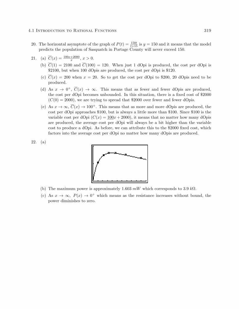
22. (a)

(b) The maximum power is approximately 1.603 mW which corresponds to 3.9 kΩ.

(c) As x → ∞, P (x) → 0+ which means as the resistance increases without bound, thepower diminishes to zero.

Section 4.1: Introduction to Rational Functions, from College … … · · 2017-11-01Chapter 4....

Documents

Transcript of Section 4.1: Introduction to Rational Functions, from College … … · · 2017-11-01Chapter 4....