1

Section 14: Electrical Energy ManagementBill Brown, P.E., Square D Engineering Services

IntroductionElectricity is a powerful form of energy that is essential to the operation of virtually every facility in the world. It is also an expensive form of energy that can represent a significant portion of a manufacturing facility’s cost of production.

This energy management primer is intended to introduce some electricity billing fundamentals, especially focusingon the two major aspects of the electric bill, demand and energy. This section also highlights key aspects ofidentifying energy-saving opportunities among major industrial processes and equipment.

Electricity billing basicsMost electric utilities serve a designated geographic territory, largely without other competitors having access to their customers. As such, utility prices have often been set by local, state, or federal regulators, entities that review electric utility costs, revenues, investment decisions, fuel prices, and other factors to arrive at a target rate of return. This approved rate of return, coupled with the utility’s cost structure, determine pricescustomers will pay.

These prices are established in electric utility tariffs, or rate schedules. Rate tariffs are usually established for different classes or sizes of customers. Common class types may include industrial, commercial, residential,municipal, and agricultural. Each customer class may have one or more rate schedules available, and it iscommon for the electric utility to allow a facility to choose the rate schedule within its class that offers the lowest price.

� Electricity metering: Electric utilities meter both the real and reactive power consumption of a facility. The realpower consumption, and its integral – energy, usually comprise the largest portion of the electric bill. Reactivepower requirements, usually expressed in power factor, can also be a significant cost and will be discussed later.

� Demand: Real power consumption, typically expressed in kilowatts or megawatts, varies instantaneously overthe course of a day as facility loads change. While instantaneous power fluctuations can be significant, electricutilities have found that average power consumption over a time interval of 15, 30, or 60 minutes is a betterindicator of the “demand” on electrical distribution equipment.

Transformers, for example, can be selected based on average power requirements of the load. Short-durationfluctuations in load current may cause corresponding drops in load voltage, but these drops are within thenormal operating tolerances of typical machines and within the design parameters of the transformer.

The demand rate, in $/kW, may also be referred to as a capacity charge, since it has historically been related tothe necessary construction of new generating stations, transmission lines, and other utility capital projects.Demand charges often represent 40% or more of an industrial customer’s monthly bill.

2

� Energy: The other major component of an electric bill is energy. The same metering equipment that measurespower demand also records customer energy consumption. Energy consumption is reported in kilowatt-hours ormegawatt-hours. Unlike power demand with its capacity relationship, customer energy consumption issometimes related to fuel requirements in electric utility generating stations. The cost per kilowatt-hour in a given electric utility rate structure, therefore, is often influenced by the mix of generating plant types in the utility system. Coal, fuel oil, natural gas, hydroelectric, and nuclear are typical fuel sources on which powergeneration is based.

� Load factor – Demand/energy relationship: One useful parameter to calculate each month is the ratio ofthe average demand to the peak demand. This unit-less number is a useful parameter that tracks theeffectiveness of demand management techniques. A load factor of 100% means that the facility operated at the same demand the entire month, a so-called “flat” profile. This type of usage results in the lowest unit cost of electricity.

Few facilities operate at a load factor of 100%, and that is not likely to represent an economical goal for mostfacilities. But a facility can calculate its historical load factor, and seek to improve it by reducing usage at peaktimes, moving batch processes to times of lower demand, and so forth. Load factor can be calculated fromvalues reported on practically every electric bill:

LF = kWh/(kW * days * 24);

Where LF is Load Factor, kWh is the total energy consumption for the billing period, kW is the peak demand setduring the billing period, and days is the number of billing days in the month (typically 28-32). “24,” of course isthe number of hours in a day.

Time-of-Use customers may prefer to track load factor only during on-peak time periods. In that case, the kWh,kW, days, and hours/day in the formula are changed to reflect the parameters established only during the on-peak periods.

Typical load factor for an industrial facility depends to a great degree on the number of shifts the plant operates.One shift, five-day operations typical record a load factor of 20-30%, while two-shifts yield 40-50%, and threeshift, 24/7 facilities may reach load factors of 70-90%.

“Demand” is the average instantaneous power consumption over a set time interval, usually 15, 30, or 60 minutes.

TIME

DEMAND

Area under curve = ENERGY (KWh)Area under line = ENERGY (KWh)

DEMAND

(For the interval defined)

Demand for each interval = Average Power over that interval

DEMANDINTERVAL

DEMANDINTERVAL

DEMANDINTERVAL

DEMANDINTERVAL

PO

WE

R (K

ILO

WA

TTS

)

INSTANTANEOUSPOWER

3

� Power factor: The relationship of real, reactive, and total power has been introduced previously, and describedas the “power triangle.” For effective electricity cost reduction, it is important to understand how the customer’selectric utility recoups its costs associated with reactive power requirements of its system. Many utilities includepower factor billing provisions in rate schedules, either directly in the form of penalties, or indirectly in the form ofreal-power billing demand that is higher than the actual measured peak.

Even if a utility does not charge directly for poor power factor, there are at least three other reasons that acustomer may find it economical to install equipment to improve power factor within its facility, thereby reducingthe reactive power requirements of the utility. PowerLogic® Solutions, volume 1, issue 4 (www.powerlogic.com)describes each of these cost-reduction opportunities in considerable detail.� Reduce power factor penalties

� Release capacity of an existing circuit

� Reduce heating losses associated with power distribution (often called I2R losses)

� Improve voltage regulation

Graphical comparison of facilities with dramatically different load factors. The three shift facility pro-duces an average demand that is nearly equal to its peak demand, while the average and peakdemand for the one shift facility is much less than one.

Dem

and,

kW

Dem

and,

kW

Equal EnergyUnequal Demand

T hree S hifts One S hift

Load Factor: 30% 50% 70%

Peak Demand, kW 1142 685 489

Energy Usage, kWh 250,000 250,000 250,000

Demand Cost $11,420 $6,850 $4,890

Energy Cost $10,000 $10,000 $10,000

Total Monthly Bill $21,420 $16,850 $14,890

Average Cost/kWh 8.57 6.74 5.96

Demand Cost AsPercent of Total

53% 41% 33%

4

� Typical energy auditing process:� Evaluate the current rate schedule

� Determine if other rate schedules are available

� Complete the Facility Energy Profile

� Assess no-cost/low-cost energy saving options

� Complete feasibility analysis of energy management project options

� Recommend Energy Action Plan

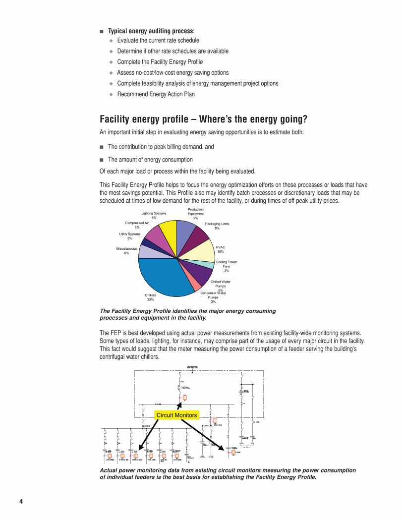
Facility energy profile – Where’s the energy going?An important initial step in evaluating energy saving opportunities is to estimate both:

� The contribution to peak billing demand, and

� The amount of energy consumption

Of each major load or process within the facility being evaluated.

This Facility Energy Profile helps to focus the energy optimization efforts on those processes or loads that havethe most savings potential. This Profile also may identify batch processes or discretionary loads that may bescheduled at times of low demand for the rest of the facility, or during times of off-peak utility prices.

The FEP is best developed using actual power measurements from existing facility-wide monitoring systems.Some types of loads, lighting, for instance, may comprise part of the usage of every major circuit in the facility.This fact would suggest that the meter measuring the power consumption of a feeder serving the building’scentrifugal water chillers.

The Facility Energy Profile identifies the major energy consuming processes and equipment in the facility.

Circuit Monitors

Actual power monitoring data from existing circuit monitors measuring the power consumptionof individual feeders is the best basis for establishing the Facility Energy Profile.

Production Equipment

9%

Packaging Lines8%

HVAC10%

Cooling Tower Fans3%

Chilled Water Pumps

9%Condenser Water

Pumps3%

Chillers33%

Miscellaneous6%

Utility Systems3%

Compressed Air8%

Lighting Systems8%

5

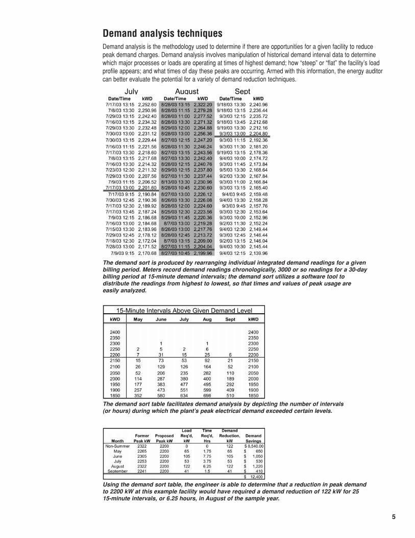
Demand analysis techniquesDemand analysis is the methodology used to determine if there are opportunities for a given facility to reducepeak demand charges. Demand analysis involves manipulation of historical demand interval data to determinewhich major processes or loads are operating at times of highest demand; how “steep” or “flat” the facility’s loadprofile appears; and what times of day these peaks are occurring. Armed with this information, the energy auditorcan better evaluate the potential for a variety of demand reduction techniques.

The demand sort is produced by rearranging individual integrated demand readings for a givenbilling period. Meters record demand readings chronologically, 3000 or so readings for a 30-daybilling period at 15-minute demand intervals; the demand sort utilizes a software tool to distribute the readings from highest to lowest, so that times and values of peak usage are easily analyzed.

The demand sort table facilitates demand analysis by depicting the number of intervals (or hours) during which the plant’s peak electrical demand exceeded certain levels.

Using the demand sort table, the engineer is able to determine that a reduction in peak demandto 2200 kW at this example facility would have required a demand reduction of 122 kW for 2515-minute intervals, or 6.25 hours, in August of the sample year.

6

Demand controlDemand controls systems are available that perform these basic functions:

� Measure power consumption (demand) in real time

� Predict demand level based on rate of instantaneous usage

� Compare predicted value to target setpoint

� Transmit signals to pre-determined equipment to turn off or curtail power usage if demand is predicted toexceed target kW

These demand controls systems are intended to reduce peak demand for a facility to some predetermined level.

The design engineer’s foremost demand control system challenge is to identify loads in the facility that can be controlled effectively. Ideal load candidates includes those machines or processes that are (1) currently contributing to the facility’s load at peak times, and (2) whose function can be delayed or curtailed at times of peak.

Most facilities lack equipment or processes that fit this ideal description, despite the numerous machines andprocesses that may be operating at peak times. In fact, successful demand control is usually the exception rather than the rule.

One common candidate for the demand control system is the air conditioning system. Buildings equipped withmultiple packaged direct-expansion air conditioning systems are typical targets of demand control sales efforts.Unfortunately, demand control of air conditioning compressors usually leads to loss of temperature or humiditycontrol within the conditioned space, or lack of demand savings.

The reason for this paradox is twofold. One, natural diversity among multiple air conditioning compressorsensures that all compressors are not operating at full load at the same time. Strangely, this fact is oftenhighlighted in the demand control system sales pitch: “Not all compressors are running at the same time, so youshould turn some off for short periods of time.”

Secondly, basic thermodynamic principles of moist air and vapor-compression refrigeration systems requirecompressor power consumption to reduce air temperature and condense moisture. This process is controlled bythermostats and humidistats within the facility. When cooling or dehumidification is removed or reduced at timeswhen these devices are “calling for” them, temperature and humidity will rise in the conditioned space.

So, if not air conditioning equipment, what loads have been successful demand control candidates? An electrolysis process providing chemicals for a paper mill was able to reduce peak demand and flatten thedemand profile for the overall facility. A battery-charging system for forklift vehicles in an automotive facility was

8000

9000

10000

11000

12000

13000

14000

15000

16000

17000

15 100

145

230

315

400

445

530

615

700

745

830

915

1000

1045

1130

1215

1300

1345

1430

1515

1600

1645

1730

1815

1900

1945

2030

2115

2200

2245

2330

Interval Ending Time (Pacific Standard Time)

Dem

and,

kW

Shoulder-Peak

Off-Peak

On-Peak

Shoulder-Peak

Off-Peak

Peak-Day load profiles from actual power monitoring data can show consistency, or, as in this case, a single-day aberration in peak demand that set the demand minimum billing level (ratchet) for the remainder of the year.

7

capable of producing real demand savings during peak times. Finally, a large induction furnace melting scrapmetal proved to be an effective candidate for the rolling mill at a steel plant.

Peak shaving with onsite generators How, the engineer might ask, can a facility save money by burning fossil fuel in an onsite generator at a unit costof 12 ¢/kWh, when the average unit cost of utility purchased power is 8 ¢/kWh? Very carefully, is the expected –and accurate – response.

The key to economical peak shaving is to understand and optimize the demand savings associated with generatoroperation. That is, the onsite generator must be operated the absolute minimum time necessary to reduce peakdemand the maximum amount. Because the overall average unit price of electricity is not necessarily equivalentto the effective price of electricity at the plant’s peak.

For example, the facility that pays an overall average unit price of 8 ¢/kWh probably pays only about 3-4 ¢/kWhfor actual energy consumption, yet an additional $10-$20/kW for demand. At the end of the month, the total billingamount divided by the total kWh usage might yield 8 ¢/kWh average, but the actual cost of power at its peak –when demand charges are included – may equate to an effective unit price of 20 ¢/kWh or higher. For the facilitywith a sharp demand peak, when the peak for the month is set in a few hours or less and the remainder of thetime demand is low, peak-shaving at 12 ¢/kWh can be preferable to paying 20 ¢/kWh.

� Costs of generated power: Onsite generators typically utilize natural gas, wood, fuel oil, or steam derivedfrom a fossil fuel or as a part of a production process. Unit fuel costs for fossil fuels are usually calculated basedon the fuel’s heating value, an estimated efficiency of the generator system, and the fuel cost.

Cost/kWh = fuel price/gal * 3413/HV/efficiency,

In this equation, HV is the heating value of fuel oil in BTU/gal, and 3413 is the conversion from BTU to kWh.Internal combustion diesel generators typically range in efficiency from 25-30%.

For a typical example, #2 fuel oil may be burned in an IC engine. For a fuel-oil price of $2.00/gal, and agenerator efficiency of 25%, the fuel cost/kWh is:

Cost/kWh = $2.00 * 3413/108,000 BTU/gal/0.25Cost/kWh = 25 ¢/kWh.

Obviously, peak-shaving is much less attractive at a fuel cost of $2.00/gal, unless required generator operationcan be predicted accurately and electricity charges are comparably high as well.

� Utility rates affecting peak-shaving generation: Electric utility rates must be analyzed carefully prior toimplementing peak shaving or cogeneration opportunities. Some utilities have special interconnection andprotective relaying requirements to ensure that onsite generation does not pose a safety hazard for utilityworkers. In addition, many utility rate schedules impose standby charges for onsite generation.

Chilled water supply and return temperatures increase over the course of a day due to demand control of inlet guide vanes on a centrifugal water chiller. Space conditions could not be maintained as a result of the demand control.

8

These charges are intended to recoup the utility’s investment in transformers and other equipment necessary toserve the facility’s entire load when the onsite generation equipment is not operating. Without this standbyequipment, utilities often reserve the right to replace service equipment with smaller facilities, at risk to thefacility of overloading the smaller equipment when onsite generation is not operating.

5 0 5 0 5 0 5 0 5 0 5 0 5 0 5 0 5 0 5 0 5 0 5 0 5 0 5 0 5 0 5 0

Plan

t Dem

and,

kW On-Peak

Period

Plant Total Power Requirement

Purchased Power

Facilities with onsite generation may be able to operate this equipment to reduce purchased powerrequirements during periods of high demand, or high utility prices.

-18%

-16%

-14%

-12%

-10%

-8%

-6%

-4%

-2%

0%

2%

4%

6000 5800 5600 5400 5200 5000 4800

Generator Setpoint, kW

$0.60/gal$0.80/gal$1.00/gal

Savings – or losses – associated with operation of peak-shaving generators is dependent on fuelprices, on-peak electricity prices, the amount of time the generator has to operate for a given peak-reduction target, and, most importantly, the accuracy with which plant personnel can predict these variables.

ProcessSteam

CondensateReturn

Turbines Electricity

Condenser

Boilers

Electricity generation and peak shaving can also be accomplished with steam cogeneration systems typical of paper mills, refineries, and other large industrial processes.

9

Lighting controlLighting systems in industrial facilities can represent an attractive savings opportunity, especially if lightingsystems have not been upgraded or maintained in the past five years. The most cost-effective approach forlighting energy savings is to address the following three issues, in order:

� Turn off lights during times when they are not needed

� Reduce light levels to match the requirements for the tasks being performed in the area

� Replace less efficient lamps, ballasts, or fixtures with more efficient sources

The second priority in lighting conservation involves light level reductions. The Illuminating Engineering Society ofNorth America (www.iesna.org) has established recommended light levels for different types of work tasks andarea usage types. In addition, it offers design guidance in laying out lighting systems, estimating light levels byzonal cavity and point-by-point lighting design methodologies.

These light level recommendations are typically described as ranges of footcandles, the footcandle being aquantity of light measured at a horizontal or vertical surface. Light output of a fixture is usually published inlumens. Many manufacturers of lamps and lighting systems offer software tools to aid in designing new systems,or in evaluating changes to existing systems.

� Some lighting essentials� Lighting controls work better than people

While “turn-off-the-light” programs have been widely utilized in all types of facilities, sophisticated lightingcontrol systems have proven to be much more cost-effective. Certainly, it’s cheaper to have a worker turn offa light, but workers forget, workers may not have access to circuit breakers controlling large banks ofindustrial lighting fixtures, those same circuit breakers are not designed for daily operation as light switches,and so on.

Lighting system controls that utilize microprocessors and specially-designed remote-operated circuitbreakers are much more effective. These devices can be programmed to accommodate complicated shiftconfigurations, including nights, weekends, and holidays. They also include simple over-ride features fortemporary or unusual work schedules. In addition, these systems can be monitored and controlled remotelyusing standard web-browser software packages, and they can interface with other control devices such asmotion sensors or photocells.

� Light levels decline with age of the lighting system.Several factors contribute to this decline. Lamps, including fluorescent and high-intensity discharge sourceslike high-pressure sodium and metal halide, experience Lamp Lumen Depreciation, or LLD. The LLD istypically less than 1.0, indicating that average lamp light output at some point in the future is less than lightoutput of a new lamp.

Power Supply

Microprocessor

Remote-OperatedCircuit Breakers

Control Bus Strips

Square D® PowerLink® lighting control panelboard utilizes patented technology to control lighting circuits, and offers Transparent Ready web-based monitoring and control. See www.powerlogic.com.

10

Light levels are also adversely affect by dirt and the accumulation of dust on the light fixture. Luminaire DirtDepreciation, or LDD, also a factor less than 1.0, is a function of the type of light fixture as well as theenvironment in which the fixture operates.

Ballast Factor, or BF, is yet another commonly used factor. BF is also a published value that is a function ofthe type of ballast used to control the arc characteristics of fluorescent and HID lighting systems.

The designer usually applies these factors to the rated light level output of a lighting system, in order toestimate the number of fixtures required to provide the desired light level – not at initial installation, rather atsome designated point in the future. For example,

# fixtures = total required lumens/initial lumens/fixture/(LLD * LDD * BF).

� Lighting designers need to know the facility’s lamp replacement practicesManufacturers publish the “rated life” expectancy of a given lamp. This value, usually given in thousands ofhours, is not a guarantee that every lamp will extinguish at the same rated-life time. In fact, the “rated life” isa statistical value indicating the point at which half of the lamps of a representative sample will burn out.Some lamps will fail well shy of the rated life; others may last beyond the rated life.

The facility’s lamp replacement practices usually fall into one of two categories:

1. Replace individual lamps as they fail (“spot replacement”)

2. Replace all lamps at a predetermined point in time, even though many of those lamps are still burning (“group replacement”)

Group replacement runs counter to common sense for most people – if it ain’t broke, don’t fix it. That’s whyspot replacement is the most common practice by far. There is, however, a sound reason for considering thegroup-replacement strategy: Economics.

If the lighting designer knows, for example, that a facility will adopt the practice of group replacement, thedesigner can utilize fewer light fixtures at the outset. That’s because the lamps replaced before their end oflife produce considerably more lumens than those allowed to burn to failure. The designer can use a higherLLD in the initial light fixture calculations to achieve the same target footcandle level.

Fewer light fixtures means lower energy costs attributable to lighting, and less heat for the building’s airconditioning system. Labor costs have also been shown to be lower for group replacement as compared tospot replacement. Group replacement can be scheduled to occur during unoccupied times; set up and takedown costs are reduced; the cost per lamp itself can be lower with large-quantity purchases.

Electric motorsThree-phase squirrel-cage induction motors comprise a considerable percentage of the electrical load in theUnited States. Design, operation, and maintenance of these machines is well described in other references; thisdocument focuses on their energy efficiency aspects.

Induction motors typically range in full load efficiency from about 87% to 94%. This efficiency is very difficult tomeasure accurately in the field, requiring a dynamometer and other specialized equipment. Fortunately, energysaving projects associated with electric motors do not require actual efficiency of a given motor to be established.

One of the foremost opportunities for energy savings is to implement a program of replacing – rather thanrewinding – induction motors at failure. Rewinding a damaged induction motor is a common practice in industry,but studies have proven that rewinding an induction motor drops its efficiency by a couple percentage points.Multiple rewinds can further reduce the efficiency of the rewound motor.

While a drop in efficiency from 89% to 88% seems insignificant, a quick estimate reveals that this reduction canbe costly. A standard efficiency 20 hp motor operating 8000 hours annually, for example, costs about $7000 per

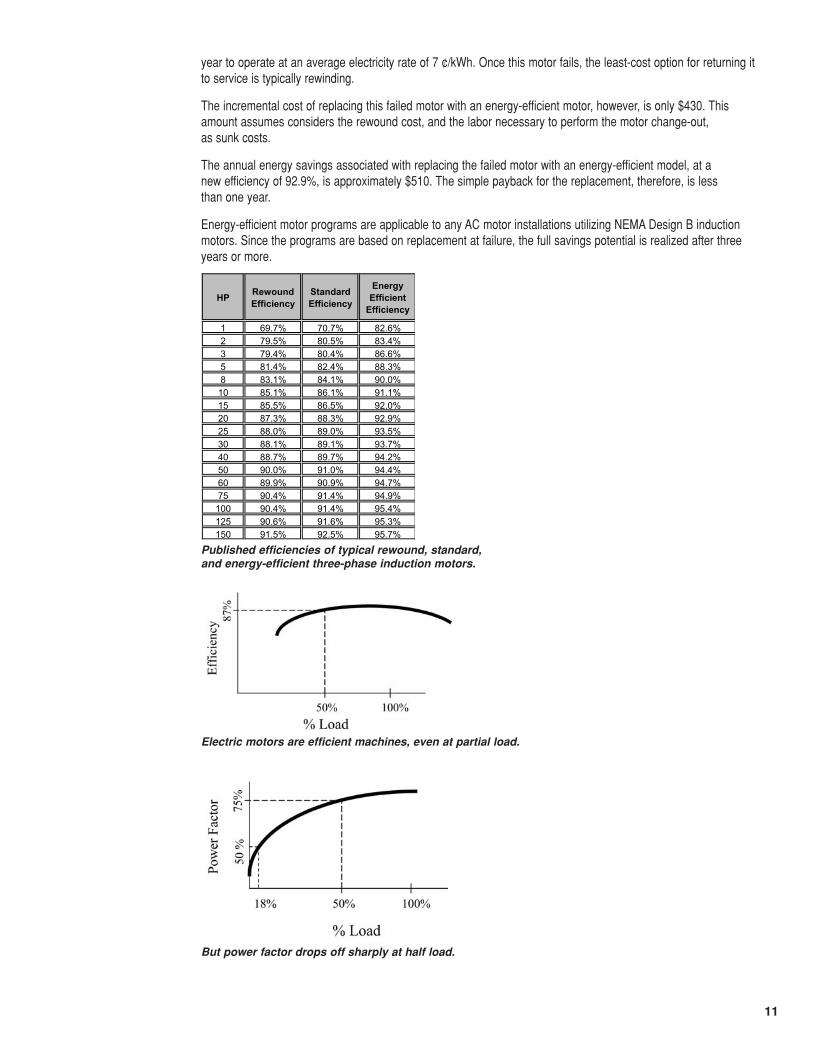
11

year to operate at an average electricity rate of 7 ¢/kWh. Once this motor fails, the least-cost option for returning itto service is typically rewinding.

The incremental cost of replacing this failed motor with an energy-efficient motor, however, is only $430. Thisamount assumes considers the rewound cost, and the labor necessary to perform the motor change-out, as sunk costs.

The annual energy savings associated with replacing the failed motor with an energy-efficient model, at a new efficiency of 92.9%, is approximately $510. The simple payback for the replacement, therefore, is less than one year.

Energy-efficient motor programs are applicable to any AC motor installations utilizing NEMA Design B inductionmotors. Since the programs are based on replacement at failure, the full savings potential is realized after threeyears or more.

HP Rewound

EfficiencyStandard Efficiency

Energy Efficient

Efficiency

1 69.7% 70.7% 82.6%2 79.5% 80.5% 83.4%3 79.4% 80.4% 86.6%5 81.4% 82.4% 88.3%8 83.1% 84.1% 90.0%10 85.1% 86.1% 91.1%15 85.5% 86.5% 92.0%20 87.3% 88.3% 92.9%25 88.0% 89.0% 93.5%30 88.1% 89.1% 93.7%40 88.7% 89.7% 94.2%50 90.0% 91.0% 94.4%60 89.9% 90.9% 94.7%75 90.4% 91.4% 94.9%100 90.4% 91.4% 95.4%125 90.6% 91.6% 95.3%150 91.5% 92.5% 95.7%

Published efficiencies of typical rewound, standard, and energy-efficient three-phase induction motors.

Electric motors are efficient machines, even at partial load.

But power factor drops off sharply at half load.

12

Variable-speed drivesThere are many devices used to provide AC motor control – starting, stopping, changing speed, varying torque,providing protection from voltage and current anomalies. This section will focus, however, on variable-frequencycontrol devices designed to reduce energy consumption and improve operation of three-phase AC inductionmotors. See www.squared.com for technical publications that describe these devices in greater detail.

AC motor loads are typically grouped in four major categories:

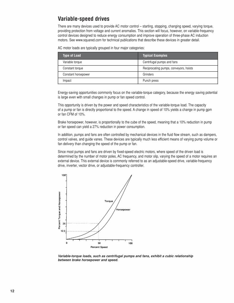
Energy-saving opportunities commonly focus on the variable-torque category, because the energy saving potentialis large even with small changes in pump or fan speed control.

This opportunity is driven by the power and speed characteristics of the variable-torque load. The capacity of a pump or fan is directly proportional to the speed. A change in speed of 10% yields a change in pump gpm or fan CFM of 10%.

Brake horsepower, however, is proportionally to the cube of the speed, meaning that a 10% reduction in pump or fan speed can yield a 27% reduction in power consumption.

In addition, pumps and fans are often controlled by mechanical devices in the fluid flow stream, such as dampers,control valves, and guide vanes. These devices are typically much less efficient means of varying pump volume orfan delivery than changing the speed of the pump or fan.

Since most pumps and fans are driven by fixed-speed electric motors, where speed of the driven load isdetermined by the number of motor poles, AC frequency, and motor slip, varying the speed of a motor requires anexternal device. This external device is commonly referred to as an adjustable-speed drive, variable-frequencydrive, inverter, vector drive, or adjustable-frequency controller.

Type of Load Typical Examples

Variable torque Centrifugal pumps and fans

Constant torque Reciprocating pumps, conveyors, hoists

Constant horsepower Grinders

Impact Punch press

Variable-torque loads, such as centrifugal pumps and fans, exhibit a cubic relationship between brake horsepower and speed.

13

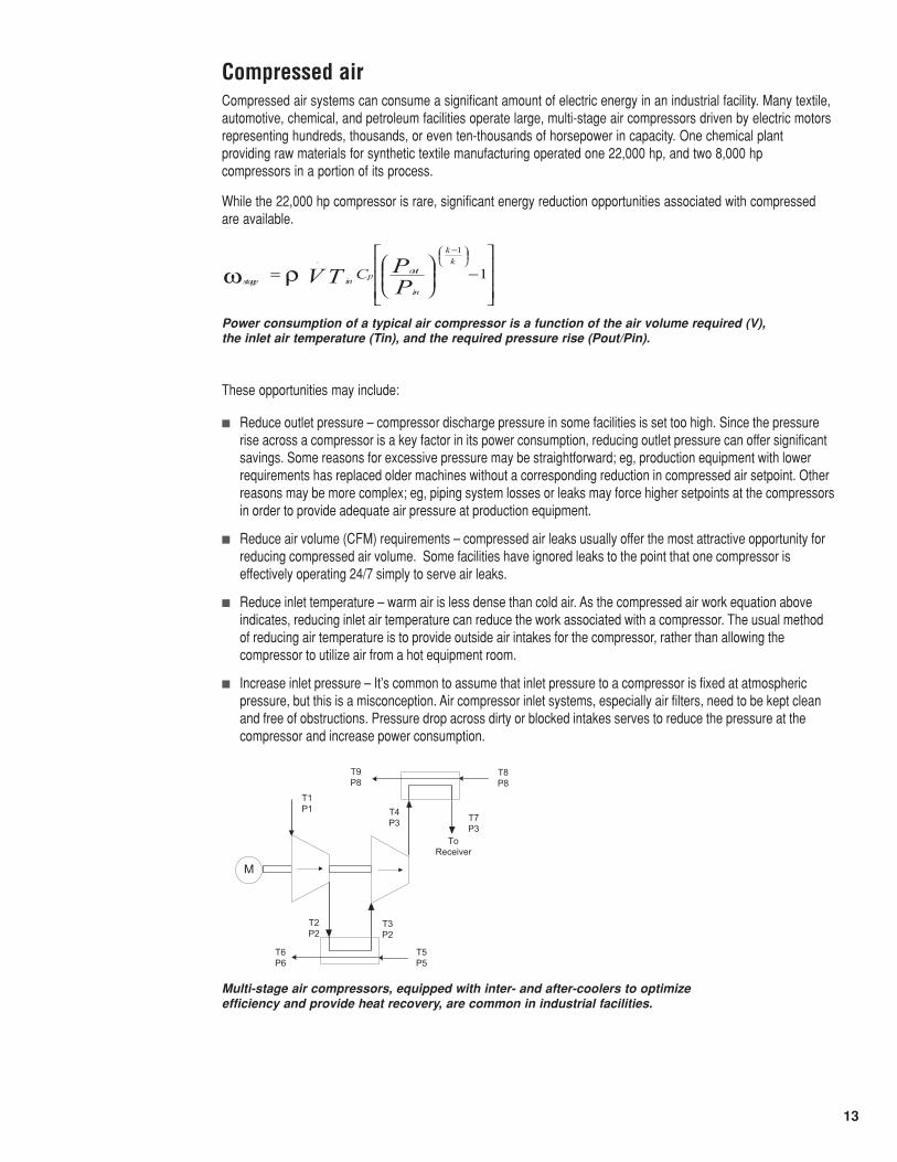
Compressed airCompressed air systems can consume a significant amount of electric energy in an industrial facility. Many textile,automotive, chemical, and petroleum facilities operate large, multi-stage air compressors driven by electric motorsrepresenting hundreds, thousands, or even ten-thousands of horsepower in capacity. One chemical plantproviding raw materials for synthetic textile manufacturing operated one 22,000 hp, and two 8,000 hpcompressors in a portion of its process.

While the 22,000 hp compressor is rare, significant energy reduction opportunities associated with compressedare available.

These opportunities may include:

� Reduce outlet pressure – compressor discharge pressure in some facilities is set too high. Since the pressurerise across a compressor is a key factor in its power consumption, reducing outlet pressure can offer significantsavings. Some reasons for excessive pressure may be straightforward; eg, production equipment with lowerrequirements has replaced older machines without a corresponding reduction in compressed air setpoint. Otherreasons may be more complex; eg, piping system losses or leaks may force higher setpoints at the compressorsin order to provide adequate air pressure at production equipment.

� Reduce air volume (CFM) requirements – compressed air leaks usually offer the most attractive opportunity forreducing compressed air volume. Some facilities have ignored leaks to the point that one compressor iseffectively operating 24/7 simply to serve air leaks.

� Reduce inlet temperature – warm air is less dense than cold air. As the compressed air work equation aboveindicates, reducing inlet air temperature can reduce the work associated with a compressor. The usual methodof reducing air temperature is to provide outside air intakes for the compressor, rather than allowing thecompressor to utilize air from a hot equipment room.

� Increase inlet pressure – It’s common to assume that inlet pressure to a compressor is fixed at atmosphericpressure, but this is a misconception. Air compressor inlet systems, especially air filters, need to be kept cleanand free of obstructions. Pressure drop across dirty or blocked intakes serves to reduce the pressure at thecompressor and increase power consumption.

Power consumption of a typical air compressor is a function of the air volume required (V), the inlet air temperature (Tin), and the required pressure rise (Pout/Pin).

Multi-stage air compressors, equipped with inter- and after-coolers to optimize efficiency and provide heat recovery, are common in industrial facilities.

14

Centrifugal water chillersCentrifugal water chillers comprise a significant portion of industrial and large commercial electrical load. These machines are efficient, typically producing a cooling effect two-to-three times greater than the requiredenergy input. Centrifugal water systems were the focus of cholorfluorocarbon (CFC) legislation in the 1980 thatdrove the replacement or reconditioning of many of these machines. Opportunities still exist, however, for chilleroptimization.

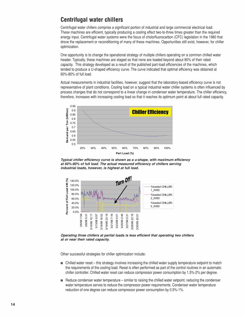
One opportunity is to change the operational strategy of multiple chillers operating on a common chilled waterheader. Typically, these machines are staged so that none are loaded beyond about 80% of their rated capacity. This strategy developed as a result of the published part-load efficiencies of the machines, which tended to produce a U-shaped efficiency curve. The curve indicated that optimal efficiency was obtained at 60%-80% of full load.

Actual measurements in industrial facilities, however, suggest that the laboratory-based efficiency curve is notrepresentative of plant conditions. Cooling load on a typical industrial water chiller systems is often influenced byprocess changes that do not correspond to a linear change in condenser water temperature. The chiller efficiency,therefore, increases with increasing cooling load so that it reaches its optimum point at about full rated capacity.

Other successful strategies for chiller optimization include:

� Chilled water reset – this strategy involves increasing the chilled water supply temperature setpoint to match the requirements of the cooling load. Reset is often performed as part of the control routines in an automaticchiller controller. Chilled water reset can reduce compressor power consumption by 1.5%-2% per degree.

� Reduce condenser water temperature – similar to raising the chilled water setpoint, reducing the condenserwater temperature serves to reduce the compressor power requirements. Condenser water temperaturereduction of one degree can reduce compressor power consumption by 0.5%-1%.

0.5

0.550.6

0.650.7

0.750.8

0.850.9

0.95

20% 30% 40% 50% 60% 70% 80% 90% 100%

Part Load (%)

Dem

and

per

Ton

(kW

/ton)

Chiller Efficiency

Typical chiller efficiency curve is shown as a u-shape, with maximum efficiency at 60%-80% of full load. The actual measured efficiency of chillers serving industrial loads, however, is highest at full load.

0.0%

20.0%40.0%60.0%

80.0%100.0%120.0%140.0%

3/6/

98 7

:58

3/8/

98 5

:31

3/10

/98

15:1

7

3/13

/98

9:57

3/16

/98

16:5

2

3/19

/98

23:1

9

3/21

/98

7:16

3/23

/98

5:01

3/25

/98

2:46

3/27

/98

0:31

3/28

/98

22:1

6

3/30

/98

20:0

1Perc

ent o

f Ful

l Loa

d kW

(%)

%loaded CHILLER-1_KWD

%loaded CHILLER-2_KWD

%loaded CHILLER-5_KWD

Operating three chillers at partial loads is less efficient that operating two chillers at or near their rated capacity.

15

� Monitor and maintain chiller approach temperatures – chiller condensers and evaporators are shell-and-tubeheat exchangers that require periodic maintenance to maintain optimum heat transfer characteristics. Sincewater travels through the condenser and evaporator tubes, solids have a tendency to accumulate on internaltube surfaces, requiring annual “rodding” to remove the scale and restore heat transfer coefficients.

Heating, ventilating, and air conditioning systemsHVAC systems should be the focus of a targeted energy study, with similar objectives as the lighting analysis:

� Turn off unnecessary HVAC equipment during unoccupied times� Match HVAC operation, including temperature and humidity, to minimum occupancy requirements� Replace inefficient HVAC systems and equipment with energy-saving alternatives

WAGESWAGES is the acronym for the complete power and energy monitoring system in a typical industrial facility.Industrials are concerned about the costs of Water, Air (compressed), Gas (natural gas), Electricity, and Steam.These systems are often interrelated to the degree that reductions in one utility can increase usage in another.The power monitoring system used by industrials has to have the capability of monitoring each of theseparameters accurately, and of posting this information in a common, preferably web-based, format for use by thelocal site and by remote engineers and managers.

Annual average readings of condenser approach temperature (difference in temperature between condenser water and refrigerant in shell-and-tube heat exchanger) gradually crept up from the initial design value of 6 F to nearly 15 F over three years.

Effect of Scale on Compressor Horsepower

100%

105%

110%

115%

120%

125%

130%

135%

140%

145%

Clean 0.001 0.002 0.003 0.004

Condenser Fouling Factor

Rela

tive

HP p

er T

on

Source: Carrier System Design Manual, Carrier Air Conditioning Co, 1963.

137% Additional Power Required!

Est'd FF = 0.0034

Increase in condenser tube fouling can have a significant adverse effect on compressor power consumption.

Web-based power monitoring systems allows energy managers to monitor the results of their demand and energy reduction techniques through the internet, and facilitate identification of new opportunities.

16

Energy survey checklist

Lighting1. Lighting operating more hours than needed?

� Reduce operating hours with lighting control system.

2. Areas over lit for task performed?� Reduce light levels by disconnecting or replacing lamps or fixtures.

3. Incandescent or quartz lamps operating more than 2,000 hours per year?� Convert to fluorescent or other energy efficient source.

4. Mercury vapor lamps.� Convert to energy saving fluorescent, metal halide, or high-pressure sodium.

5. Standard fluorescent lamps operating one shift.� Convert to energy saving fluorescent lamps and ballasts.

6. Standard fluorescent lamps operating two or three shifts.� Convert to energy saving fluorescent lamps and ballasts.

7. Fluorescent at 18-feet or higher mounting heights.� Convert to high pressure sodium.

8. VHO fluorescent fixtures.� Convert to energy saving fluorescent, metal halide, or high pressure sodium.

9. Standard fluorescent ballasts.� Replace with energy savings electronic ballasts at failure.

Induction motors1. Motors operating 75%+ full load, more than 6,000 hours per year.

� Replace with energy efficient motors at failure.

2. Standard V-belts on pumps or fans.� Convert to cog V-belts.

3. Fans or pumps that are throttled with dampers or control valves.� Consider variable speed drives.

Demand management1. Sharp demand peaks of short duration (low load factor)?

� Identify loads to shed or reschedule to off-peak.

2. Batch processes? � Shift to off-peak.

3. Consider Time-of-Use savings opportunities.

Exhaust, ventilation, and pneumatic conveying1. Transport velocities or exhaust flows higher than minimum required?

� Consider changing belts and sheaves to reduce air velocity.

2. Consider variable speed or inlet vane control.

17

3. Consider exhaust air heat recovery.

4. Make-up air properly provided for all exhaust?

5. Fume hoods designed to minimize exhaust?

6. Properly designed stack heads (no Chinese hats or caps on outlets)

Fan-coil unit air handling units1. Consider air side economizers.

2. Considered chilled water reset.

3. Consider water side economizer.

Centrifugal water chillers1. Multiple chillers operating on a common header.

� Fully load one chiller before starting another.

2. Consider chilled water reset.

3. Consider water side economizer.

4. Consider variable speed chiller control (long hours at light loads).

5. Excessive approach temperatures – Check trends or design data.� Clean condenser and evaporator tubes.

6. Adding cooling load or chillers?� Consider thermal energy storage.

Cooling towers1. Consider variable speed drives for fan motors.

2. Consider PVC fill to replace wood fill material.

3. Consider velocity recovery stacks.

Boilers1. Stack gas temperature > 400 F? (Ideal temperature: 100 degrees plus saturation temperature of the steam)

� Consider economizer to preheat feedwater or combustion air.

2. Manual or intermittent blowdown?� Consider automatic blowdown system.

3. Continuous blowdown?� Consider blowdown heat recovery system.

4. Excess air high or unburned combustibles?� Consider boiling tuning.

5. Large amounts of high pressure condensate?� Consider high pressure condensate receiver.

6. Increase amount of condensate returned.

7. Improve boiler chemical treatment.

8. Maintain steam traps.

18

Heat recovery1. Waste water streams > 100 F?

� Consider heat exchanger and/or heat pump.

2. Waste air or gas stream > 300 F?� Consider heat exchanger.

Cogeneration1. Boiler rated pressure 100 psi greater than pressure required by process?

2. Concurrent steam and electrical demands?� Consider back-pressure turbine.

Refrigeration1. Consider hot gas heat recovery.

2. Consider thermal storage.

Compressed air1. Provide additional small air compressor for loads.

2. Provide outside air intake.

3. Eliminate air leaks.