Section 1: Introduction, Probability Concepts and Decisions

Section 1: Introduction,Probability Concepts and Decisions

Carlos M. Carvalho and Robert McCulloch

Readings:OpenIntro Statistics, Chapters 2 and 3

1

Course Overview

Section 1: Introduction, Probability Concepts and Decisions

Section 2: Learning from Data: Estimation, Confidence Intervals and

Testing Hypothesis

Section 3: Simple Linear Regression

Section 4: Multiple Linear Regression

Section 5: Topics in Regression

Section 6: Naive Bayes

2

Let’s start with a question...

My entire portfolio is in U.S. equities. How would you describe the

potential outcomes for my returns by the end of the year?

3

Another question... (Target Marketing)

Suppose you are deciding whether or not to target a customer with

a promotion(or an add)...

It will cost you $.80 (eighty cents) to run the promotion and a

customer spends $40 if they respond to the promotion.

Should you do it ???

4

Introduction

Probability and statistics let us talk about things we are unsure

about.

I How much will Amazon sell next quarter?

I What will the return of my retirement portfolio be next year?

I How often will users click on a particular Facebook ad?

I If I give a patient a certain drug, how long are they likely to

live?

I Will the Leafs win the Stanley Cup any time soon?

All of these involve inferring or predicting unknown quantities!!

5

Random Variables

I Random Variables are numbers that we are NOT sure about

but we might have some idea of how to describe its potential

outcomes.

I Example: Suppose we are about to toss two coins.

Let X denote the number of heads.

We say that X , is the random variable that stands for the

number we are not sure about.

6

Probability Distribution

I We describe the behavior of random variables with a


I Example: If X is the random variable denoting the number of

heads in two coin tosses, we can describe its behavior through

the following probability distribution:

x P(X = x)

0 .25

1 .5

2 .25

x : a possible outcome

P(X = x): the probability X turns out to be x .

7


I X is called a Discrete Random Variable as we are able to list

all the possible outcomes

I Question: What is P(X = 0)? How about P(X ≥ 1)?

8

The Bernoulli Distribution

A very common situation is that we are wondering whether

something will happen or not.

Heads or tails, respond or don’t respond, .....

It turns out to be very convenient to code up one possibility as a 0,

and the other possibility as a 1.

The gives us the Bernoulli distribution.

X ∼ Bernoulli(p) means:

x P(X = x)

0 1-p

1 p

9

Example:

I am about to toss a single coin. X is the random variable which is

1 if the coin turns out to be heads and 0, if it is tails.

X ∼ Bernoulli(.5)

Example:

L is the random variable which is 1 if the Leafs win the Stanley

Cup and 0, if not.

L ∼ Bernoulli(?????)

10

Conditional, Joint and Marginal Distributions

In general we want to use probability to address problems involving

more than one variable at the time.

Let’s suppose you are thinking about your sales next quarter.

Let S denote your sales (in thousands of units sold).

S is a number you are not sure about !!

In thinking about what S , you find you are thinking about what

will happen next quarter for the overall economy.

We need to think about two things we are uncertain about, the

economy and sales!

11

Let E denote the performance of the economy next quarter.

Let E = 1 if the economy is expanding and E = 0 if the economy

is contracting (what kind of random variable is this?).

Let’s assume P(E = 1) = 0.7.

12

Let S denote my sales next quarter... and let’s suppose the

following probability statements:

S P(S |E = 1) S P(S |E = 0)

1 0.05 1 0.20

2 0.20 2 0.30

3 0.50 3 0.30

4 0.25 4 0.20

These are called Conditional Distributions, they describe our beliefs

about S conditional on knowing what happens for E .

13

S P(S |E = 1) S P(S |E = 0)

1 0.05 1 0.20

2 0.20 2 0.30

3 0.50 3 0.30

4 0.25 4 0.20

I In blue is the conditional distribution of S given E = 1

I In red is the conditional distribution of S given E = 0

I We read: the probability of Sales of 4 (S = 4) given(or

conditional on) the economy is growing (E = 1) is 0.25

14

The conditional distributions tell us about about what can happen

to S for a given value of E ... but what about S and E jointly?

P(S = 4 and E = 1) = P(E = 1)× P(S = 4|E = 1)

= 0.70× 0.25 = 0.175

In english, 70% of the times the economy grows and 1/4 of those

times sales equals 4... 25% of 70% is 17.5%

15

>IJP37Q

>IKP&$6%Q

AIX

AI

AIW

AIJ

AIX

AI

AIW

AIJ

/0

/1

/2

/2

/1

/1

/23

/3

/2

/43

5"#$%&'()&*$+,&$&/0-/23&$&/+03&

5"#$1&'()&*$+,&$&/0-/3&$&/13

5"#$2&'()&*$+,&$&/0-/2&$&/+%&

5"#$+&'()&*$+,&$&/0-/43&$&/413&

5"#$%&'()&*$4,&$&/1-/2&$&/46

5"#$1&'()&*$4,&$&/1-/1 $&/47

5"#$2&'()&*$4,&$&/1-/1 $&/47

5"#$+&'()&*$4,&$&/1-/2&$&/46

49)("'1"(95"'()*"#(% ]PAIXQ"M

95.5"'1")"&'17*)8$B"(95"69$*57.$<511@

N95.5").5"^"7$11'2*5$3(<$=51"B$."PA+>Q

!JRV_!K`

16

We can specify the distribution of the pair of random variables

(S ,E ) by listing all possible pairs and the corresponding probability.

(s, e) p(S = s,E = e)

(1,1) .035

(2,1) .14

(3,1) .35

(4,1) .175

(1,0) .06

(2,0) .09

(3,0) .09

(4,0) .06

Question: What is P(S = 1) ?

17

We call the probabilities of E and S together the joint distribution

of E and S .

In general the notation is...

I P(Y = y ,X = x) is the joint probability of the random

variable Y equal y AND the random variable X equal x .

I P(Y = y |X = x) is the conditional probability of the random

variable Y takes the value y GIVEN that X equals x .

I P(Y = y) and P(X = x) are the marginal probabilities of

Y = y and X = x

18

Warning:

The notation can get tricky.

Sometimes rather than writing

P(X = x ,Y = y)

someone might write just,

p(x , y)

for the same thing!!

Usually, but not always, capitals are used for random variables and

small case is used for possible values.19

Conditional, Joint and Marginal Distributions and

Two-way TablesWhy we call marginals marginals... the table represents the joint

and at the margins, we get the marginals.

>?)=7*5"A")%&">")/)'%

45"<)%"&'17*)8"(95"a$'%("&'1(.'23('$%"$B"A")%&">"31'%/)"(6$"6)8"()2*5!

N95"5%(.8"'%"(95"1"<$*3=%")%&"5".$6"/';51"]PAI1")%&">I5Q!

A

J"""""""W""""""" """""""X

>K"""!K`""""!Kb""""!Kb !K`

J"""!K V""!JX""""! V""""!JRV

!

!R

!KbV"""!W """!XX""""!W V J

T$6"8$3"<)%155"698"(95=)./'%)*1).5"<)**5&(95"=)./'%)*1!

20

Conditionals from Joints

We derived the joint distribution of (E , S) from the marginal for E

and the conditional S | E .

You can also calculate the conditional from the joint by doing it

the other way

P(Y = y ,X = x) = P(X = x) P(Y = y | X = x)

⇒

P(Y = y | X = x) =P(Y = y ,X = x)

P(X = x)

21

Example... Given E = 1 what is the probability of S = 4?

A

J"""""""W""""""" """""""X

>K"""!K`""""!Kb""""!Kb !K`

J"""!K V""!JX""""! V""""!JRV

!

!R

!KbV"""!W """!XX""""!W V J

>?)=7*5

! !"# ! $#! "

7PA +> Q !7PA U> Q !

7P> Q !

i';5%">"3769)("'1"(957.$2 A)*51IXM

PB.$="(95"a$'%(&'1(.'23('$%Q

P(S = 4|E = 1) =P(S = 4,E = 1)

P(E = 1)=

0.175

0.7= 0.25

22

Example... Given S = 4 what is the probability of E = 1?

A

J"""""""W""""""" """""""X

>K"""!K`""""!Kb""""!Kb !K`

J"""!K V""!JX""""! V""""!JRV

!

!R

!KbV"""!W """!XX""""!W V J

! !"#! " # $%#

7PA +> Q !7P> U A Q !

7PA Q !

i';5%"1)*51IX+69)("'1"(957.$2)2'*'(8(95%">"'1"37M

P(E = 1|S = 4) =P(S = 4,E = 1)

P(S = 4)=

0.175

0.235= 0.745

23

Independence

Two random variable X and Y are independent if

P(Y = y |X = x) = P(Y = y)

for all possible x and y .

In other words,

knowing X tells you nothing about Y !

e.g.,tossing a coin 2 times... what is the probability of getting H in

the second toss given we saw a T in the first one?

24

Example:

You are about to toss two coins.

Let X1 be 1 if the first coin is a head and 0 if tails.

Let X2 be 1 if the second coin is a head and 0 if tails.

X1 ∼ Bernoulli(.5), X2 ∼ Bernoulli(.5)

25

What is the probability of getting two heads in a row?

P(X1 = 1,X2 = 1) = P(X1 = 1) P(X2 = 1 | X1 = 1)

= P(X1 = 1) P(X2 = 1)

= (.5)× (.5)

= .25

26

IID

Our two coins X1 and X2 both have the same distribution and they

are independent.

We say they are IID:

I I: independent

I ID: identically distributed

This terminology gets used a lot in statistics.

27

Example:

We say the two coins are IID Bernoulli with p = .5.

Suppose I am about to toss two dice.

Y1 is the number on the face of the first die.

Y2 is the number on the face of the second die.

Are Y1, Y2 IID?

Are Y1, Y2 IID Bernoulli?

28

Bayes Theorem

Disease Testing Example

Let D = 1 indicate you have a disease

Let T = 1 indicate that you test positive for it

>?)=7*5

0'15)15"(51('%/!

H5("0"IJ"'%&'<)(5"8$3"9);5"(95"&'15)15!H5("NIJ"'%&'<)(5"(9)("8$3"(51("7$1'(';5"B$."'(!

-$1("&$<($.1"(9'%:"'%"(5.=1"$B"7P&Q")%&"7P(U&Q!

/42

/7G

0IJ

0IK

NIJ

NIK

/73

/43

NIJ

NIK

/4+

/77

"

0

K""""""""""""""""""""""""J

NK"""!bRKWI!b^Z!bb"""""!KKJ

J"""!KKb^""""""""""""""""""!KJb

If you take the test and the result is positive, you are really

interested in the question: Given that you tested positive, what is

the chance you have the disease?29

F3("'B"8$3").5"(95"7)('5%("69$"(51(1"7$1'(';5"B$.)"&'15)15"8$3"<).5")2$3("]P0IJUNIJQ"P7P&U(QQ!

0K""""""""""""""""""""""""J

NK"""!bRKW""""""""""""""""""!KKJ

J"""!KKb^""""""""""""""""""!KJb

]P0IJUNIJQ"I"!KJb¥P!KJb_!KKb^Q"I"K!``

+,"-.#/&!0/$.1$/2!1"$"-.3/45($61/$5./75(#7./&!05(-./$5./8"1.(1.9+

P(D = 1|T = 1) =0.019

(0.019 + 0.0098)= 0.66

30

Note:

In this example the sensitivity is .95.

The probability of a true postitive.

In this example the specificity is .99.

The probability of a true negative.

31

Bayes Theorem:

In the disease testing problem we formulated our understand of the

variable T and D using

p(t, d) = p(d)p(t|d).

Then we use probability theory to compute the quantity we really

want which is

p(d | t).

This process of getting the probability “the other way” from how

the modeling describes things is called Bayes Theorem.

32

We can develop of more formal statement of Bayes Theorem by

writing things out using our basic properties of probability.

Suppose we have p(y) and p(x | y).

p(y |x) =p(y , x)

p(x)=

p(y , x)∑y p(y , x)

=p(y)p(x |y)∑y p(y)p(x |y)

For binary y (y is 0 or 1, as in our Disease testing problem), we

have:

p(Y = 1|x) =p(Y = 1) p(x |Y = 1)

p(Y = 0) p(x |Y = 0) + p(Y = 1) p(x |Y = 1)

33

More Than Two Random Variables

Of course, we may want to think about more than two uncertain

quantities at a time!!

Our ideas extend nicely to any number of variables.

For example with three random variables X1, X2, and X3 we might

want to think about:

P(X1 = x1,X2 = x2,X3 = x3)

The probability that X1 turns out to be x1 and X2 turns out to be

x2 and X3 turns out to be x3.

35

We can immediately extend our basic inutitive ideas:

P(X1 = x1,X2 = x2,X3 = x3) =

P(X1 = x1) P(X2 = x2 | X1 = x1) P(X3 = x3 | X1 = x1,X2 = x2).

36

Example:

Suppose we have 10 voters.

4 are republican and 6 are democratic.

We “randomly” choose 3.

Let Yi be 1 if the i th voter is a democrat and 0 otherwise,

i = 1, 2, 3.

What is

P(Y1 = 1,Y2 = 1,Y3 = 1)

What is the probability of getting three democrats in a row ??

37

P(Y1 = 1,Y2 = 1,Y3 = 1) =

P(Y1 = 1) p(Y2 = 1 | Y1 = 1) P(Y3 = 1 | Y1 = 1,Y2 = 1)

= (6/10)(5/9)(4/8)

= (1/6) = .167.

38

When we randomly pick a person from a population of people, and

then randomly pick a second from the ones left, and so on, we call

it sampling without replacement.

If we put the person back each time and randomly choose from the

whole group each time, then we call it sampling with replacement.

39

Random Sampling in R

> set.seed(99)

> sample(1:10,5)

[1] 6 2 10 7 4

> sample(1:10,5)

[1] 10 7 3 8 2

> set.seed(99)

> sample(1:10,5)

[1] 6 2 10 7 4

> sample(1:10000,20)

[1] 9667 6714 2946 3583 1753 5486 5052 1938 6364 6872 6396 3575 1025 977 1827

[16] 2276 804 8203 5901 7720

> sample(1:10,5,replace=TRUE)

[1] 4 1 9 1 3

40

Example:

Suppose we are tossing 100 coins.

Let Xi be 1 if the ith coin is a head and 0 otherwise.

What is the probability of 100 heads in a row?

P(X1 = 1,X2 = 1, . . . ,X100 = 1) =

P(X1 = 1)P(X2 = 1 | X1 = 1) . . .P(Xj = 1 | X1 = 1,X2 = 1, . . . ,Xj−1 = 1)

. . .P(X100 = 1 | X1 = 1, . . . ,X99 = 1)

= .5100 = 7.888609e − 31.

The 100 Xi are IID Bernoulli, with p = .5.

41

Question:

Suppose I get 100 heads in a row.

What is the probability the next one is a head?

42

Example:

Suppose I toss 100 dice.

Let Yi be number on the ith die.

Are the Yi IID?

Are the Yi IID Bernoulli?

43

Probability and Decisions

Suppose you are presented with an investment opportunity in the

development of a drug... probabilities are a vehicle to help us build

scenarios and make decisions.

You make a 1 million invest-

ment to develop the drug.

If “no cure” (drug does not

work) you get 250,000 back

you don’t spend.

If you do find a cure you have

to worry about whether it is ap-

proved and whether a competi-

tor beats you out.

44

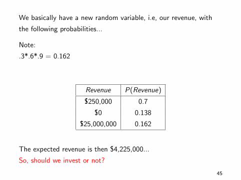
We basically have a new random variable, i.e, our revenue, with

the following probabilities...

Note:

.3*.6*.9 = 0.162

Revenue P(Revenue)

$250,000 0.7

$0 0.138

$25,000,000 0.162

The expected revenue is then $4,225,000...

So, should we invest or not?

45

Back to Target Marketing

Should we send the promotion ???

Well, it depends on how likely it is that the customer will respond!!

If they respond, you get 40-0.8=$39.20.

If they do not respond, you lose $0.80.

Let’s assume your “predictive analytics” team has studied the

conditional probability of customer responses given customer

characteristics... (say, previous purchase behavior, demographics,

etc)

46

Suppose that for a particular customer, the probability of a

response is 0.05.

Profit P(Profit)

$-0.8 0.95

$39.20 0.05

Should you do the promotion?

.95*(-.8) + .05*39.20 = 1.2.

Homework question: How low can the probability of a response be

so that it is still a good idea to send out the promotion?

47

Let’s get back to the drug investment example...

What if you could choose this investment instead?

Revenue P(Revenue)

$3,721,428 0.7

$0 0.138

$10,000,000 0.162

The expected revenue is still $4,225,000...

What is the difference?

48

Here is a plot of the two distribution for the two drug discovery

scenarios.

0.0e+00 5.0e+06 1.0e+07 1.5e+07 2.0e+07 2.5e+07

0.2

0.3

0.4

0.5

0.6

0.7

Revenue

prob

abili

ty

First scenario

Second scenario

49

Mean and Variance of a Random Variable

The Mean or Expected Value is defined as (for a discrete X ):

E (X ) =n∑

i=1

P(xi )× xi

We weight each possible value by how likely they are... this

provides us with a measure of centrality of the distribution... a

“good” prediction for X !

50

Suppose

X =

{1 with prob. p

0 with prob. 1− p

E (X ) =n∑

i=1

P(xi )× xi

= 0× (1− p) + 1× p

E (X ) = p

51

The Variance is defined as (for a discrete X ):

Var(X ) =n∑

i=1

P(xi )× [xi − E (X )]2

Weighted average of squared prediction errors... This is a measure

of spread of a distribution. More risky distributions have larger

variance.

52

Suppose

X =

{1 with prob. p

0 with prob. 1− p

Var(X ) =n∑

i=1

P(xi )× [xi − E (X )]2

= (0− p)2 × (1− p) + (1− p)2 × p

= p(1− p)× [(1− p) + p]

Var(X ) = p(1− p)

Question: For which value of p is the variance the largest?

53

The Standard Deviation

I What are the units of E (X )? What are the units of Var(X )?

I A more intuitive way to understand the spread of a

distribution is to look at the standard deviation:

sd(X ) =√

Var(X )

I What are the units of sd(X )?

54

Mean and Variance for Drug Development Example

Previously we computed the expected value for the drug

development examples.

Let’s review those calculations and compute the variances as well.

Same mean,

Different

standard deviations!!

> pv = c(.7,.138,.162)

>

> d1 = c(250000,0,25000000)

> d2 = c(3721428,0, 10000000)

>

> cat("E1:",sum(pv*d1),"\n")

E1: 4225000

> cat("E2:",sum(pv*d2),"\n")

E2: 4225000

>

> M = sum(pv*d1)

>

> v1 = sum(pv*(d1-M)^2)

> v2 = sum(pv*(d2-M)^2)

> s1 = sqrt(v1)

> s2 = sqrt(v2)

>

> cat("s1,s2: ",s1,", ",s2,"\n")

s1,s2: 9134721 , 2836141

55

Covariance

I A measure of dependence between two random variables...

I It tells us how two unknown quantities tend to move together

The Covariance is defined as (for discrete X and Y ):

Cov(X ,Y ) =n∑

i=1

m∑j=1

P(xi , yj)× [xi − E (X )]× [yj − E (Y )]

I What are the units of Cov(X ,Y ) ?

56

Example:

µX = .1, µY = .1.

σX = .05, σY = .05.

X

.05 .15

.05 .4 .1

Y

.15 .1 .4

x y prob x-E(X) y-E(Y) prod

0.05 0.05 0.4 -0.05 -0.05 0.0025

0.15 0.05 0.1 0.05 -0.05 -0.0025

0.05 0.15 0.1 -0.05 0.05 -0.0025

0.15 0.15 0.4 0.05 0.05 0.0025

Cov(X ,Y ) = σXY

= .4 ∗ .0025 + .1 ∗ (−.0025) + .1 ∗ (−.0025) + .4 ∗ .0025 = .0015.

Intuition: There is an 80% chance X and Y move in the same direction.57

Example:

µX = .1, µY = .1.

σX = .05, σY = .05.

X

.05 .15

.05 .1 .4

Y

.15 .4 .1

x y prob x-E(X) y-E(Y) prod

0.05 0.05 0.1 -0.05 -0.05 0.0025

0.15 0.05 0.4 0.05 -0.05 -0.0025

0.05 0.15 0.4 -0.05 0.05 -0.0025

0.15 0.15 0.1 0.05 0.05 0.0025

Cov(X ,Y ) = σXY

= .1 ∗ .0025 + .4 ∗ (−.0025) + .4 ∗ (−.0025) + .1 ∗ .0025 = −.0015.

Intuition: There is an 80% chance X and Y move in opposite directions.58

Ford vs. Tesla

I Assume a very simple joint distribution of monthly returns for

Ford (F ) and Tesla (T ):

t=-7% t=0% t=7% P(F=f)

f=-4% 0.06 0.07 0.02 0.15

f=0% 0.03 0.62 0.02 0.67

f=4% 0.00 0.11 0.07 0.18

P(T=t) 0.09 0.80 0.11 1

Let’s summarize this table with some numbers...

59

t=-7% t=0% t=7% P(F=f)

f=-4% 0.06 0.07 0.02 0.15

f=0% 0.03 0.62 0.02 0.67

f=4% 0.00 0.11 0.07 0.18

P(T=t) 0.09 0.80 0.11 1

I E (F ) = 0.12, E (T ) = 0.14

I Var(F ) = 5.25, sd(F ) = 2.29, Var(T ) = 9.76, sd(T ) = 3.12

I What is the better stock?

60

t=-7% t=0% t=7% P(F=f)

f=-4% 0.06 0.07 0.02 0.15

f=0% 0.03 0.62 0.02 0.67

f=4% 0.00 0.11 0.07 0.18

P(T=t) 0.09 0.80 0.11 1

Cov(F ,T ) =(−7− 0.14)(−4− 0.12)0.06 + (−7− 0.14)(0− 0.12)0.03+

(−7− 0.14)(4− 0.12)0.00+(0− 0.14)(−4− 0.12)0.07+

(0− 0.14)(0− 0.12)0.62 + (0− 0.14)(4− 0.12)0.11+

(7− 0.14)(−4− 0.12)0.02 + (7− 0.14)(0− 0.12)0.02+

(7− 0.14)(4− 0.12)0.07 = 3.063

Okay, the covariance in positive... makes sense, but can we get a

more intuitive number?61

Correlation

Corr(X ,Y ) =Cov(X ,Y )

sd(X )sd(Y )

I What are the units of Corr(X ,Y )? It doesn’t depend on the

units of X or Y !

I −1 ≤ Corr(X ,Y ) ≤ 1

In our first example:

Corr(X,Y) = .0015/(.05*.05) = 0.6

In our second example:

Corr(X,Y) = -.0015/(.05*.05) = -0.6

62

In our Ford vs. Tesla example:

Corr(F ,T ) =3.063

2.29× 3.12= 0.428 (not too strong!)

63

Linear Combination of Random Variables

Is it better to hold Ford or Tesla? How about half and half?

What do we mean by “half and half”?

We mean the portfolio where we put half of our money into Ford

and half into Tesla.

Return On a Portfolio:

Suppose we form a portfolio in which we put fraction w1 of our

wealth into an asset with return R1 and fraction w2 of our wealth

into an asset with return R2. Let P be the return on the portfolio.

P = w1 R1 + w2 R2

64

In our Ford/Tesla use use R1 = Ford, R2 = Tesla, and

w1 = w2 = .5.

Since the return on Ford and Tesla are random variables, so of

course is the return on the portfolio!

Here is the joint distribution of (R1,R2) = (F ,T ) and

P = .5 F + .5 T .

Ford Tesla P prob

1 -4 -7 -5.5 0.06

2 0 -7 -3.5 0.03

3 4 -7 -1.5 0.00

4 -4 0 -2.0 0.07

5 0 0 0.0 0.62

6 4 0 2.0 0.11

7 -4 7 1.5 0.02

8 0 7 3.5 0.02

9 4 7 5.5 0.07

65

Is it better to hold Ford or Tesla? How about half and

half?

We can compare the random returns based on the means and

variances:

big mean: good, big variance: bad.

We could could compute the mean and variance of P directly from

its distribution, but there are some very handy formulas for the

mean and variance of a linear combination of random variables.

Let X and Y be two random variables, a, b, and c are known

constants:

I E (c + aX + bY ) = c + aE (X ) + bE (Y )

I Var(c +aX +bY ) = a2Var(X )+b2Var(Y )+2ab×Cov(X ,Y )66

Applying this to the Ford vs. Tesla example...

I E (0.5F + 0.5T ) = 0.5E (F ) + 0.5E (T ) =

0.5× 0.12 + 0.5× 0.14 = 0.13

I Var(0.5F + 0.5T ) =

(0.5)2Var(F ) + (0.5)2Var(T ) + 2(0.5)(0.5)× Cov(F ,T ) =

(0.5)2(5.25) + (0.5)2(9.76) + 2(0.5)(0.5)× 3.063 = 5.28

I sd(0.5F + 0.5T ) =√

5.28 = 2.297

so, what is better? Holding Ford, Tesla or the combination?

asset: Ford, Tesla, Portfolio

mean: .12, .14, .13

sd: 2.29, 3.12, 2.297

67

Let’s check the mean and variance of P from our basic formulas bycomputing them in R.

> head(ddf)

Ford Tesla P prob

1 -4 -7 -5.5 0.06

2 0 -7 -3.5 0.03

3 4 -7 -1.5 0.00

4 -4 0 -2.0 0.07

5 0 0 0.0 0.62

6 4 0 2.0 0.11

> EP = sum(ddf$prob * ddf$P)

> cat("Expected value of port: ",EP,"\n")

Expected value of port: 0.13

> VP = sum(ddf$prob * (ddf$P-EP)^2)

> cat("Variance of port: ",VP,"\n")

Variance of port: 5.2931

Same numbers!!

68

Let’s see what is going on graphically!I plot the three distributions for Ford, Tesla, and the portfolio

I possible values on the x axis, probabilities on the y axis

I easy to see that Tesla has a higher variance than Ford.

I not so easy to see the difference in the means, this is realistic

I you can see you the diversification killed the tails

−6 −4 −2 0 2 4 6

0.0

0.2

0.4

0.6

0.8

outcomes

prob

abili

ty

● PortfolioFordTesla

●●

●

●

●

●

●

●●

69

Note:

If X and Y are independent, then Cov(X ,Y ) = 0.

Covariance measures linear dependence.

If they have nothing to do with each other (independence), then

they certainly have nothing to do with each other linearly.

70

More generally...

I E (w0 + w1X1 + w2X2 + ...wpXp) =

w0+w1E (X1)+w2E (X2)+...+wpE (Xp) = w0 +∑p

i=1 wiE (Xi )

I Var(w0+w1X1+w2X2+...wpXp) = w 21 Var(X1)+w 2

2 Var(X2)+

...+w 2pVar(Xp)+2w1w2×Cov(X1,X2)+2w1w3Cov(X1,X3)+

... =∑p

i=1 w 2i Var(Xi ) +

∑pi=1

∑j 6=i wiwjCov(Xi ,Xj)

71

Example:

Ford, Tesla, GM.

P = w1F + w2T + w3G

E (P) = w1E (F ) + w2E (T ) + w3E (G )

Var(P) = w 21 Var(F ) + w 2

2 Var(T ) + w 23 Var(G )

+ 2w1w2Cov(F ,T ) + 2w1w3Cov(F ,G ) + 2w2w3Cov(T ,G ).

72

With lots of assests this gets complicated!! There many possible

pairs of assests and corresponding covariance pairs representing the

high dimensional dependence of the many input assets.

In practice you have to estimate all the covariances from data,

another good reason to index!!

73

Example, Sum and Mean of IID

Suppose you play a game n times and the winning from the ith

play is represented by the random variable Xi , i = 1, 2, . . . , n.

We assume the each play of the game is indepedent of the others

and it is the same game each time.

So, the Xi are IID.

What are the mean and variance of the total winnings?

T = X1 + X2 + X3 + . . .+ Xn.

Let E (Xi ) = µ and Var(Xi ) = σ2.

74

T = X1 + X2 + X3 + . . .+ Xn.

The Mean:

E (T ) = E (X1) + E (X2) + . . .+ E (Xn)

= µ+ µ+ . . .+ µ

= n µ

The variance:

For the variance note that Because all the Xi are independent, the

covariances are all 0 !!!!!

Var(T ) = Var(X1) + Var(X2) + . . .+ Var(Xn)

= σ2 + σ2 + . . .+ σ2

= n σ2

75

And the average:

X̄ =1

nX1 +

1

nX2 +

1

nX3 + . . .+

1

nXn.

The Mean:

E (X̄ ) =1

nE (X1) +

1

nE (X2) + . . .+

1

nE (Xn)

=1

nµ+

1

nµ+ . . .+

1

nµ

= n (1

n)µ = µ

76

X̄ =1

nX1 +

1

nX2 +

1

nX3 + . . .+

1

nXn.

The variance:

Var(X̄ ) =1

n2Var(X1) +

1

n2Var(X2) + . . .+

1

n2Var(Xn)

=1

n2σ2 +

1

n2σ2 + . . .+

1

n2σ2

= n (1

n2)σ2

=σ2

n.

77

Note:

We have, for Xi , IID, E (Xi ) = µ, Var(Xi ) = σ2,

E (X̄ ) = µ, Var(X̄ ) =σ2

n.

Intuitively this says the average of a lot of IID draws tends to be

closer to the mean µ than an individual draw.

We do a lot of averaging in statistics !!

This will turn out to be important !!

78

Portfolio vs. Single Project (from Misbehaving)

In a meeting with 23 executives plus the CEO of a major company

economist Richard Thaler poses the following question:

Suppose you were offered an investment opportunity for your

division (each executive headed a separate/independent division)

that will yield one of two payoffs. After the investment is made,

there is a 50% chance it will make a profit of $2 million, and a

50% chance it will lose $1 million. Thaler then asked by a show of

hands who of the executives would take on this project. Of the

twenty-three executives, only three said they would do it.

79

Then Thaler asked the CEO a question. If these projects were

independent, that is, the success of one was unrelated to the

success of another, how many of the projects would he want to

undertake? His answer: all of them!

What ?????!!!!

How can we understand this?

80

for an individual executive:

Xi , i = 1, 2, . . . , 23.

x P(X = x)

-1 .5

2 .5

µ: .5 ∗ (−1) + .5 ∗ 2 = 0.5

σ2: .5 ∗ (−1− .5)2 + .5 ∗ (2− .5)2 = 2.25

σ: 1.5

µ/σ: .5/1.5 = 0.3333333

81

for CEO:

T = X1 + X2 + X3 + . . .+ Xn.

E (T ): 23*.5 = 11.5

Var(T ) : 23*2.25 = 51.75

sd(T ): sqrt(51.75) = 7.193747

E (T )/sd(T ): 11.5/7.193747 = 1.598611

For the CEO, the mean is much bigger relative to the standard

deviation that is it for the individual managers !!!

82

Companies, CEO’s, managers have to be careful in setting

incentives that avoid what psychologist and behavior economists

call “narrow framing”... otherwise, what can be perceived to be

bad for one manager may be very good for the entire company!

83

Continuous Random Variables

I Suppose we are trying to predict tomorrow’s return on the

S&P500...

I Question: What is the random variable of interest?

I Question: How can we describe our uncertainty about

tomorrow’s outcome?

I Listing all possible values seems like a crazy task... we’ll work

with intervals instead.

I These are called continuous random variables.

I The probability of an interval is defined by the area under the

probability density function, the “pdf”.

84

The Normal Distribution

I A random variable is a number we are NOT sure about but

we might have some idea of how to describe its potential

outcomes.

I The probability the number ends up in an interval is given by

the area under the curve (pdf)

This is the pdf

for the

standard normal

distribution.

−4 −2 0 2 4

0.0

0.1

0.2

0.3

0.4

z

stan

dard

nor

mal

pdf

85

Notation: We often use Z , to denote a standard normal random

variable.

P(−1 < Z < 1) = 0.68

P(−1.96 < Z < 1.96) = 0.95

−4 −2 0 2 4

0.0

0.1

0.2

0.3

0.4

z

stan

dard

nor

mal

pdf

−4 −2 0 2 4

0.0

0.1

0.2

0.3

0.4

z

stan

dard

nor

mal

pdf

86

Note:

For simplicity we will often use P(−2 < Z < 2) ≈ 0.95

Questions:

I What is P(Z < 2) ? How about P(Z ≤ 2)?

I What is P(Z < 0)?

87

I The standard normal is not that useful by itself. When we say

“the normal distribution”, we really mean a family of

distributions.

I We obtain pdfs in the normal family by shifting the bell curve

around and spreading it out (or tightening it up).

88

I We write X ∼ N(µ, σ2).

I The parameter µ determines where the curve is. The center of

the curve is µ.

I The parameter σ determines how spread out the curve is. The

area under the curve in the interval (µ− 2σ, µ+ 2σ) is 95%.

P(µ− 2σ < X < µ+ 2σ) ≈ 0.95

x

µµ µµ ++ σσ µµ ++ 2σσµµ −− σσµµ −− 2σσ

89

I For the normal family of distributions we can see that the

parameter µ talks about “where” the distribution is located or

centered.

I We often use µ as our best guess for a prediction.

I The parameter σ talks about how spread out the distribution

is. This gives us and indication about how uncertain or how

risky our prediction is.

I Z ∼ N(0, 1).

90

Example:

I Below are the pdfs of

X1 ∼ N(0, 1), X2 ∼ N(3, 1), and X3 ∼ N(0, 16).

I Which pdf goes with which X ?

−8 −6 −4 −2 0 2 4 6 8

91

Mean and Variance of a Continuous Random Variable

Continuous random variables have expected values and variances

analogous to what we have defined for discrete random variables.

But, the definition requires calculus and we don’t want to have to

remember all that stuff.

Fortunately, our intuition is the same!!!

I The expected value of a random variable is the probability

weighted average value.

I The variance of a random variable is the probability weighted

average squared distance to the expected value.

92

Mean and Variance for a Normal

For

X ∼ N(µ, σ2),

E (X ) = µ, Var(X ) = σ2

µ is the mean and σ2 is the variance !!

Note:

E (Z ) = 0, Var(Z ) = 1.

93

The Normal Distribution – Example

I Assume the annual returns on the SP500 are normally

distributed with mean 6% and standard deviation 15%.

SP500 ∼ N(6, 225). (Notice: 152 = 225).

I Two questions: (i) What is the chance of losing money on a

given year? (ii) What is the value that there’s only a 2%

chance of losing that or more?

I Lloyd Blankfein: “I spend 98% of my time thinking about 2%

probability events!”

I (i) P(SP500 < 0) and (ii) P(SP500 <?) = 0.02

94

The Normal Distribution – Example

−40 −20 0 20 40 60

0.00

00.

010

0.02

0

sp500

prob less than 0

−40 −20 0 20 40 60

0.00

00.

010

0.02

0

sp500

prob is 2%

(i) P(SP500 < 0) = 0.35 and (ii) P(SP500 < −25) = 0.02

95

In R:

For X ∼ N(µ, σ2), pnorm(c,...) gives P(X < c), which is the

CDF (cumulative distribution function) evaluated at c .

qnorm(q,...) gives the value c such that P(X < c) = q.

> 1-2*pnorm(-1.96,mean=0,sd=1)

[1] 0.9500042

> 1-2*pnorm(-1.00,mean=0,sd=1)

[1] 0.6826895

> pnorm(0,mean=6,sd=15)

[1] 0.3445783

> pnorm(-25,mean=6,sd=15)

[1] 0.01938279

>

> qnorm(.02,mean=6,sd=15)

[1] -24.80623

In Excel see: NORMDIST and NORMINV 96

The Probability of an Interval:

What is P(0 < SP500 < 20) ?

That is, what is the probability that the return value ends up being

in the interval (0, 20)?

> pnorm(0,6,15)

[1] 0.3445783

> pnorm(20,6,15)

[1] 0.8246761

> 0.8246761 - 0.3445783

[1] 0.4800978

The probability of the interval (a, b) is CDF (b)− CDF (a).

97

Standardization

X ∼ N(µ, σ2)

µ is the mean and σ2 is the variance.

Standardization: if X ∼ N(µ, σ2) then

Z =X − µσ

∼ N(0, 1)

X−µσ should look like a Z !!

The number of standard deviations, X is away from the mean.

98

Example:

Prior to the 1987 crash, monthly S&P500 returns (R) followed

(approximately) a normal with mean 0.012 and standard deviation

equal to 0.043. How extreme was the crash of -0.2176? The

standardization helps us interpret these numbers...

R ∼ N(0.012, 0.0432)

The month of the crash, R turned out to be r = −0.2176.

Correspondingly, for the crash,

z =−0.2176− 0.012

0.043= −5.27

which is pretty wild for a standard normal!!

5 standard deviations away from the mean!! 99

The Normal Distribution – Approximating Combinations of RVs

Recall the Thaler example (Portfolios of projects vs. single project).

A linear combination of independent random variables is

approximately normal (the CLT: Central Limit Theorm), so

T ∼ N(11.5, 7.22) approximately> .5 * 23

[1] 11.5

> 2.25*23

[1] 51.75

> sqrt(51.75)

[1] 7.193747

> 1 - pnorm(0,11.5,7.2)

[1] 0.9448919−10 0 10 20 30 40

0.00

0.01

0.02

0.03

0.04

0.05

Total

much more compelling than the simple Sharpe ratio we looked at before !!

100

In summary, in many situations, if you can figure out the mean and

variance of the random variable of interest, you can use a normal

distribution to approximate the calculation of probabilities.

101

Portfolios, once again...

I As before, let’s assume that the annual returns on the SP500

are normally distributed with mean 6% and standard deviation

of 15%, i.e., SP500 ∼ N(6, 152)

I Let’s also assume that annual returns on bonds are normally

distributed with mean 2% and standard deviation 5%, i.e.,

Bonds ∼ N(2, 52)

I What is the best investment?

I What else do I need to know if I want to consider a portfolio

of SP500 and bonds?

102

I Additionally, let’s assume the correlation between the returns

on SP500 and the returns on bonds is -0.2.

I How does this information impact our evaluation of the best

available investment?

Recall that for two random variables X and Y :

I E (aX + bY ) = aE (X ) + bE (Y )

I Var(aX + bY ) = a2Var(X ) + b2Var(Y ) + 2ab × Cov(X ,Y )

I One more very useful property... sum of normal random

variables is a new normal random variable!

103

I What is the behavior of the returns of a portfolio with 70% in

the SP500 and 30% in Bonds?

I E (0.7SP500 + 0.3Bonds) = 0.7E (SP500) + 0.3E (Bonds) =

0.7× 6 + 0.3× 2 = 4.8

I Var(0.7SP500 + 0.3Bonds) =

(0.7)2Var(SP500) + (0.3)2Var(Bonds) + 2(0.7)(0.3)×Corr(SP500,Bonds)× sd(SP500)× sd(Bonds) =

(0.7)2(152) + (0.3)2(52) + 2(0.7)(0.3)×−0.2×15×5 = 106.2

I Portfolio ∼ N(4.8, 10.32)

104

Here are the normal pdfs for our three assets, SP500, Bonds, and

the portfolio.

−40 −20 0 20 40

0.00

0.02

0.04

0.06

0.08

return

pdf

SP500

Bonds

Portfolio

105

The Uniform Distribution

Suppose we think a random variable X can turn out to be any

number between -.25 and .25 and the numbers in (-.25,25) are

equally likely?

How would we describe this??

Suppose we think a random variable X can turn out to be any

number between 0 and 1 and the numbers are equally likely?

How would we describe this?

106

If X can be any number in (a, b) and the numbers are equally

likely, then we say X ∼ Uniform(a, b)

−0.5 0.0 0.5 1.0

0.0

0.5

1.0

1.5

2.0

x

f(x)

X~Uniform(−.25,.25)

X~Uniform(0,1)

The density is 1b−a inside (a, b) and 0 elswhere.

107

Section 1: Introduction, Probability Concepts and Decisions

Documents

Transcript of Section 1: Introduction, Probability Concepts and Decisions