SecondEdition - Technical University of Denmark · October 14, 2015 14:45 WSPC/Book Trim Size for...
192
October 14, 2015 14:45 WSPC/Book Trim Size for 9in x 6in newFAEntHilbSpace Second Edition FUNCTIONAL ANALYSIS: Entering Hilbert Space Vagn Lundsgaard Hansen Publishers’ page i
Transcript of SecondEdition - Technical University of Denmark · October 14, 2015 14:45 WSPC/Book Trim Size for...
October 14, 2015 14:45 WSPC/Book Trim Size for 9in x 6in newFAEntHilbSpace
Second Edition
FUNCTIONAL ANALYSIS:
Entering Hilbert Space
Vagn Lundsgaard Hansen
Publishers’ page
i

October 14, 2015 14:45 WSPC/Book Trim Size for 9in x 6in newFAEntHilbSpace
Publishers’ page
ii

October 14, 2015 14:45 WSPC/Book Trim Size for 9in x 6in newFAEntHilbSpace
Publishers’ page
iii

October 14, 2015 14:45 WSPC/Book Trim Size for 9in x 6in newFAEntHilbSpace
Publishers’ page
iv

October 14, 2015 14:45 WSPC/Book Trim Size for 9in x 6in newFAEntHilbSpace
To my students
v

October 14, 2015 14:45 WSPC/Book Trim Size for 9in x 6in newFAEntHilbSpace
vi
October 14, 2015 14:45 WSPC/Book Trim Size for 9in x 6in newFAEntHilbSpace
Preface
Second Edition
In the second edition, I have expanded the material on normed vector spaces
and their operators presented in Chapter 1 to include proofs of the Open Map-
ping Theorem, the Closed Graph Theorem and the Hahn-Banach Theorem.
The material on operators between normed vector spaces is further ex-
panded in a new chapter on Fredholm theory (Chapter 6). Fredholm theory
originates in pioneering work of the Swedish mathematician Erik Ivar Fred-
holm on integral equations, which inspired the study of a new class of bounded
linear operators, known as Fredholm operators. Chapter 6 presents the basic
elements of the theory of Fredholm operators on general Banach spaces, not
only on Hilbert spaces, since this is important for applications of the theory.
The more general setting with Banach spaces requires that we develop the
theory of dual operators between Banach spaces to replace the use of adjoint
operators between Hilbert spaces.
Fredholm operators are of interest far beyond mathematical analysis, they
also play a significant role in theoretical physics, differential geometry and
topology with the famous Index Theorem proved by Michael Atiyah and
Isadore Singer in 1963 as a highlight.
With the addition of the new material on normed vector spaces and their
operators, the book can hopefully serve as a general introduction to functional
analysis viewed as a theory of infinite dimensional linear spaces and linear
operators acting on them.
Technical University of Denmark, 2015
Vagn Lundsgaard Hansen
vii

October 14, 2015 14:45 WSPC/Book Trim Size for 9in x 6in newFAEntHilbSpace
viii Functional Analysis: Entering Hilbert Space

October 14, 2015 14:45 WSPC/Book Trim Size for 9in x 6in newFAEntHilbSpace
Preface ix
First Edition
Functional analysis is one of the important new mathematical fields from the
twentieth century. It originates from the calculus of variations in the study of
operators on function spaces defined by differentiation and integration. The
name functional analysis was coined by the French mathematician Paul Levy
(1886–1971). Early pioneers were Italian Vito Volterra (1860–1940), Swedish
Erik Ivar Fredholm (1866–1927), German David Hilbert (1862–1943) and Hun-
garian Frigyes Riesz (1880–1956). The Polish mathematician Stefan Banach
(1892–1945) was influential in bringing the notions of topology into functional
analysis, and he is known for the seminal book Theorie des operations lineaires
of 1932. Fundamental contributions to the study of operators on Hilbert spaces
were made by the Hungarian mathematician John von Neumann (1903–57).
Inspiration to this work came from many sides, not least from the develop-
ment of quantum mechanics in physics in the 1920s by physicists such as Niels
Bohr (1885–1962), Paul Dirac (1902–84), Werner K. Heisenberg (1901–76) and
Erwin Schrodinger (1887–1961).
The present book supplements my earlier book Fundamental Concepts
in Modern Analysis, World Scientific, 1999, with an introduction to Hilbert
spaces. The new book can be read independently of the first book by readers
with a basic knowledge in general topology and normed vector spaces, including
the operator norm of a bounded linear operator. To set the stage properly we
review briefly the necessary elements of metric topology in Chapter 1. Together
the two books are used for a course at the advanced undergraduate/beginning
graduate level offered to engineering students at the Technical University of
Denmark. It is my hope that the books will also appeal to university students
in mathematics and in the physical sciences.
A fundamental problem in applications of functional analysis is connected
with the construction of suitable spaces to handle a given application. Often the
spaces needed are complete normed vector spaces (Banach spaces) constructed
from spaces of continuous functions. In this spirit, Chapter 2 opens with a
slightly novel construction of the Lp-spaces together with proofs of the basic
inequalities of Holder and Minkowski in these spaces. Other important Banach
spaces arising from function spaces and sequence spaces are also treated.
The main bulk of the book presents the basic elements of the theory of
Hilbert spaces (Chapter 3) and operators on Hilbert spaces (Chapter 4), cul-
minating in a proof of the spectral theorem for compact, self-adjoint operators
on separable Hilbert spaces (Chapter 5).
The presentation of material has been greatly influenced by ideas of my

October 14, 2015 14:45 WSPC/Book Trim Size for 9in x 6in newFAEntHilbSpace
x Functional Analysis: Entering Hilbert Space
good colleague Michael Pedersen presented in his book Functional Analysis in
Applied Mathematics and Engineering, Chapman & Hall/CRC, 2000. I appre-
ciate many joyful conversations with Michael about functional analysis and
thank him for several valuable comments to my exposition. I also like to point
out that his book contains a wealth of applications of methods from func-
tional analysis in the engineering sciences, in particular applications based on
the abstract formulations of partial differential equations in a Hilbert space
setting.
I am extremely grateful to my colleagues Preben Alsholm and Ole Jørsboe
for a very careful reading of the entire manuscript and for many valuable
suggestions.
Notions from general topology and basic elements of the theory of normed
vector spaces are in general used throughout this book without further notice.
To ease the reading of the book, a short summary of the necessary elements of
metric topology is given in Chapter 1.
Technical University of Denmark, 2006
Vagn Lundsgaard Hansen

October 14, 2015 14:45 WSPC/Book Trim Size for 9in x 6in newFAEntHilbSpace
Contents
Preface vii
Preliminary Notions 1
1. Basic Elements of Metric Topology 5
1.1 Metric spaces . . . . . . . . . . . . . . . . . . . . . . . . . . . . 5
1.2 The topology of a metric space . . . . . . . . . . . . . . . . . . 9
1.3 Completeness and compactness of metric spaces . . . . . . . . . 11
1.4 The Banach Fixed Point Theorem . . . . . . . . . . . . . . . . 15
1.5 The Baire Category Theorem . . . . . . . . . . . . . . . . . . . 17
1.6 Normed vector spaces . . . . . . . . . . . . . . . . . . . . . . . 19
1.7 Bounded linear operators . . . . . . . . . . . . . . . . . . . . . 21
1.8 The Open Mapping Theorem . . . . . . . . . . . . . . . . . . . 25
1.9 The Hahn-Banach Theorem . . . . . . . . . . . . . . . . . . . . 28
2. New Types of Function Spaces 33
2.1 Completion of metric spaces and normed vector spaces . . . . . 33
2.2 The Weierstrass Approximation Theorem . . . . . . . . . . . . 38
2.3 Important inequalities for p-norms in spaces of continuous func-
tions . . . . . . . . . . . . . . . . . . . . . . . . . . . . . . . . . 42
2.4 Construction of Lp-spaces . . . . . . . . . . . . . . . . . . . . . 46
2.4.1 The Lp-spaces and some basic inequalities . . . . . . . . 46
2.4.2 Lebesgue measurable subsets in R . . . . . . . . . . . . . 49
2.4.3 Smooth functions with compact support . . . . . . . . . 52
2.4.4 Riemann integrable functions . . . . . . . . . . . . . . . 53
2.5 The sequence spaces lp . . . . . . . . . . . . . . . . . . . . . . . 55
xi

October 14, 2015 14:45 WSPC/Book Trim Size for 9in x 6in newFAEntHilbSpace
xii Functional Analysis: Entering Hilbert Space
3. Theory of Hilbert Spaces 59
3.1 Inner product spaces . . . . . . . . . . . . . . . . . . . . . . . . 59
3.2 Hilbert spaces . . . . . . . . . . . . . . . . . . . . . . . . . . . . 64
3.3 Basis in a normed vector space and separability . . . . . . . . . 65
3.3.1 Infinite series in normed vector spaces . . . . . . . . . . 65
3.3.2 Separability of a normed vector space . . . . . . . . . . . 66
3.4 Basis in a separable Hilbert space . . . . . . . . . . . . . . . . . 68
3.5 Orthogonal projection and complement . . . . . . . . . . . . . 76
3.6 Weak convergence . . . . . . . . . . . . . . . . . . . . . . . . . 81
4. Operators on Hilbert Spaces 85
4.1 The adjoint of a bounded linear operator . . . . . . . . . . . . 85
4.2 Compact operators . . . . . . . . . . . . . . . . . . . . . . . . . 92
5. Spectral Theory 99
5.1 The spectrum and the resolvent . . . . . . . . . . . . . . . . . . 99
5.2 Spectral theorem for compact self-adjoint operators . . . . . . . 103
6. Fredholm Theory 111
6.1 Dual spaces and operators . . . . . . . . . . . . . . . . . . . . . 111
6.2 A duality theorem for operators with closed image . . . . . . . 117
6.3 Fredholm Operators . . . . . . . . . . . . . . . . . . . . . . . . 122
6.4 Topology of spaces of operators . . . . . . . . . . . . . . . . . . 130
6.5 Integral operators and integral equations . . . . . . . . . . . . . 136
6.6 Operator equations of Fredholm Type . . . . . . . . . . . . . . 141
Exercises 145
Bibliography 173
List of Symbols 175
Index 177

October 14, 2015 14:45 WSPC/Book Trim Size for 9in x 6in newFAEntHilbSpace
Preliminary Notions
There are certain standard notations and terminologies used throughout math-
ematics. In this explanatory note we list some of these.
Logical symbols
∀ for all
∃ there exists
=⇒ implies
⇐⇒ if and only if
∈ belongs to
/∈ does not belong to
⊂ proper subset
⊆ subset
∧ and
∨ or
: such that
Sets of numbers
N the set of natural numbers
Z the set of integers
Q the set of rational numbers
I the set of irrational numbers
R the set of real numbers
R+ the set of positive real numbers
R+0 the set of non-negative real numbers
C the set of complex numbers
1
October 14, 2015 14:45 WSPC/Book Trim Size for 9in x 6in newFAEntHilbSpace
2 Functional Analysis: Entering Hilbert Space
Notions from set theory
A set can be declared by listing the elements. For example,
{x | x has property P}
denotes the set of elements x with a given property P . Often the property Pwill be expressed in logical symbols as below.
∅ the empty set
A ∪B the union of sets A and B, i.e. {x | x ∈ A ∨ x ∈ B}A ∩B the intersection of sets A and B, i.e. {x | x ∈ A ∧ x ∈ B}A ⊔B the union of disjoint sets A and B,
i.e. {x | x ∈ A ∨ x ∈ B} and A ∩B = ∅⋃
α∈I
Aα the union of sets Aα indexed by
the elements α in an index set I
⋂
α∈I
Aα the intersection of sets Aα indexed by
the elements α in an index set I
A×B the product set of the sets A and B,
i.e. {(x, y) | x ∈ A, y ∈ B}
S \A the set difference, i.e. {x ∈ S | x /∈ A}
Notions related to mappings
f : A→ B a mapping of A into B
f(A) the image of f , i.e. f(A) = {b ∈ B | ∃a ∈ A : f(a) = b}
f−1(C) the preimage of subset C ⊆ B under mapping f : A→ B,
i.e. f−1(C) = {a ∈ A | f(a) ∈ C}
Relations and equivalence classes
A relation ∼ in a set S is a subset R ⊆ S × S, or in other words, a
distinguished set of ordered pairs of points x, y ∈ S. We write x ∼ y if
(x, y) ∈ R.
October 14, 2015 14:45 WSPC/Book Trim Size for 9in x 6in newFAEntHilbSpace
Preliminary Notions 3
The relation ∼ is called an equivalence relation if
(i) x ∼ x (∼ is reflexive)
(ii) x ∼ y =⇒ y ∼ x (∼ is symmetric)
(iii) (x ∼ y) ∧ (y ∼ z) =⇒ x ∼ z (∼ is transitive) .
If ∼ is an equivalence relation in S, then S can be partitioned into a corre-
sponding system of disjoint subsets, so-called equivalence classes Sα, indexed
by α ∈ I, and defined by
x, y ∈ Sα ⇐⇒ x ∼ y .
If on the other hand,
S =⊔
α∈I
Sα ,
then we can define a relation ∼ in S by
x ∼ y ⇐⇒ x, y ∈ Sα for some α ∈ I .
Clearly ∼ is an equivalence relation in S.
An equivalence relation in a set S and a partition of S into a disjoint union
of equivalence classes amounts in other words to the same thing.
If ∼ is an equivalence relation in S, the set of equivalence classes is denoted
by S = S/∼ and π : S → S denotes the mapping which associates to an
element x ∈ S its equivalence class π(x) ∈ S.
Notions related to orderings
A (partial) ordering ≤ in a set S is a relation R ⊆ S × S, where we write
x ≤ y if (x, y) ∈ R, that satisfies the following conditions:
(i) x ≤ x (≤ is reflexive)
(ii) (x ≤ y) ∧ (y ≤ x) =⇒ x = y (≤ is anti-symmetric)
(iii) (x ≤ y) ∧ (y ≤ z) =⇒ x ≤ z (≤ is transitive).
A set S together with an ordering relation is called an ordered set. In this
book, the only ordering relation we shall consider is the usual ordering ≤ in
the set of real numbers R.
Let A be a subset in the ordered set S with ordering relation ≤.
An element xmax ∈ A is called a maximal element in A if x ≤ xmax for
all x ∈ A. Similarly, an element xmin ∈ A is called a minimal element in A if
xmin ≤ x for all x ∈ A.

October 14, 2015 14:45 WSPC/Book Trim Size for 9in x 6in newFAEntHilbSpace
4 Functional Analysis: Entering Hilbert Space
An element s ∈ S is called an upper bound for A if x ≤ s for all x ∈ A. If
A is bounded from above, then an upper bound s∗ ∈ S is called a least upper
bound, or a supremum, of A, if s∗ ≤ s for all other upper bounds s ∈ S of A.
An element t ∈ S is called a lower bound for A if t ≤ x for all x ∈ A. If
A is bounded from below, then a lower bound t∗ ∈ S is called a greatest lower
bound, or an infimum, of A, if t ≤ t∗ for all other lower bounds t ∈ S of A.
October 14, 2015 14:45 WSPC/Book Trim Size for 9in x 6in newFAEntHilbSpace
Chapter 1
Basic Elements of Metric Topology
A major step forward in the development of functional analysis was taken
around 1900 when mathematicians in their search for solutions to variational
problems began to consider functions with specified properties as elements in
spaces of functions of similar type. This was enhanced by the creation of new
mathematical structures, such as metric spaces and more generally, topological
spaces, which came to be known as general, or pointset, topology. Using these
new structures a firm basis could be established for fundamental notions from
analysis such as convergence of sequences and continuity of functions.
In this introductory chapter we review briefly some basic elements of general
topology of spaces involving a metric structure. Readers already familiar with
this material may proceed immediately to Chapter 2.
1.1 Metric spaces
A distance function (or a metric) on a set M is a function d : M ×M → R
which to any pair of points x, y ∈ M associates a real number d(x, y), called
the distance from x to y. Furthermore, to get a reasonable notion of distance, it
has proved fruitful to require that the following three conditions are satisfied:
MET 1 (positive definite)
d(x, y) ≥ 0, for all x, y ∈M , = 0 ⇐⇒ x = y.
MET 2 (symmetry)
d(x, y) = d(y, x), for all x, y ∈M.
MET 3 (the triangle inequality)
d(x, z) ≤ d(x, y) + d(y, z), for all x, y, z ∈M.
5

October 14, 2015 14:45 WSPC/Book Trim Size for 9in x 6in newFAEntHilbSpace
6 Functional Analysis: Entering Hilbert Space
Definition 1.1.1. A metric on a setM is a function d :M×M → R satisfying
the conditions MET 1, MET 2, MET 3.
A pair (M,d) consisting of a set M together with a specific metric d on M
is called a metric space.
Remark 1.1.2. The same setM can be equipped with several different metrics,
in which case the corresponding metric spaces are counted as different.
When the context leaves no doubt as to which metric is being considered,
usually the metric is not mentioned explicitly.
The idea of metric spaces was introduced by the French mathematician
Maurice Frechet (1878–1973) in his doctoral thesis of 1906.
A few examples of metric spaces are in order.
Example 1.1.3. Consider the set of real n-tuples M = Rn.
For points x = (x1, . . . , xn) and y = (y1, . . . , yn) in Rn we set
d(x, y) =
√√√√n∑
i=1
(xi − yi)2 .
Clearly MET 1 and MET 2 are satisfied. To prove that MET 3 is satisfied we
need some preparations.
The space Rn is an n-dimensional real vector space with the usual coordi-
natewise definition of addition and multiplication by scalars. The points in Rn
are then identified with vectors. We define the inner product by
(x, y ) =
n∑
i=1
xiyi ,
and the associated norm by
||x || =
√√√√n∑
i=1
xi2 .
Then we have the Cauchy-Schwarz inequality:
|(x, y ) | ≤ ||x || ||y || for all x, y ∈ Rn .
Proof. Let x, y ∈ Rn be arbitrarily chosen, but fixed vectors in Rn. For
every real number t ∈ R we have the inequality
0 ≤ (x+ ty , x+ ty ) = ||y ||2t2 + 2(x, y )t+ ||x ||2 .

October 14, 2015 14:45 WSPC/Book Trim Size for 9in x 6in newFAEntHilbSpace
Chapter 1: Basic Elements of Metric Topology 7
For y 6= 0, this describes a polynomial of degree 2 in t (a parabola) with at
most one zero. Therefore, the discriminant of the polynomial must satisfy
4(x, y )2 − 4||x ||2||y ||2 ≤ 0 .
From this we get the inequality |(x, y ) | ≤ ||x || ||y || as asserted.For y = 0, the inequality is trivially satisfied. �
The Cauchy-Schwarz inequality implies the triangle inequality:
||x+ y || ≤ ||x ||+ ||y ||.
Proof. Using the Cauchy-Schwarz inequality, the small computation
||x+ y ||2 = (x + y , x+ y ) = ||x ||2 + ||y ||2 + 2(x, y )
≤ ||x ||2 + ||y ||2 + 2||x || · ||y ||= (||x ||+ ||y ||)2
reveals the triangle inequality. �
By noting that
d(x, y) = ||x− y ||,
the condition MET 3 now follows immediately:
d(x, z) = ||x − z || = ||x − y + y − z ||≤ ||x − y ||+ ||y − z || = d(x, y) + d(y, z).
Thereby we have verified that Rn equipped with the distance function d is
a metric space. This metric space is called n-dimensional Euclidean space, and
the metric d, the Euclidean metric on Rn.
For n = 1 we get the usual concept of distance on a line by identification
with R along a coordinate axis. For n = 2, 3 we rediscover the usual concept of
distance in a plane, respectively 3-dimensional space, when these are identified
with R2, respectively R3, by choosing an orthogonal coordinate system.
Before the next example, we recall a fundamental property of the system
of real numbers, namely the existence of a supremum (and infimum). Together
with the well-known algebraic properties, the existence of a supremum char-
acterizes the system of real numbers.
Property (Supremum). Every non-empty subset A of R which is bounded
from above has a smallest upper bound, which is called the least upper bound
of A, or supremum of A, and is denoted by supA.
October 14, 2015 14:45 WSPC/Book Trim Size for 9in x 6in newFAEntHilbSpace
8 Functional Analysis: Entering Hilbert Space
From the existence of a supremum we easily get:
Property (Infimum). Every non-empty subset A of R which is bounded from
below has a largest lower bound, which is called the greatest lower bound of A,
or infimum of A, and is denoted by inf A.
Example 1.1.4. For K a non-empty, but otherwise arbitrary, fixed set, letM
be the set of all bounded real-valued functions f : K → R defined on K.
For f, g ∈M put
d(f, g) = supx∈K
|f(x) − g(x) |
= sup{|f(x)− g(x) |
∣∣ x ∈ K}.
Note that since
A ={|f(x)− g(x) |
∣∣ x ∈ K}
is bounded from above, the number d(f, g) = supA exists. Note also that we
have used different ways of writing supA in the present example.
MET 1 follows since 0 ≤ |f(x) − g(x) | ≤ supA for all x ∈ K. MET 2 is
also easily seen, since |f(x)− g(x) | = |g(x)− f(x) | for all x ∈ K.
To prove that MET 3 is satisfied we proceed as follows.
Let f, g, h be three functions in M . For every x ∈ K, we then have
|f(x)− h(x) | = |f(x)− g(x) + g(x)− h(x) |≤ |f(x)− g(x) |+ |g(x) − h(x) |≤ sup
x∈K|f(x)− g(x) |+ sup
x∈K|g(x)− h(x) |
= d(f, g) + d(g, h).
From this we see that d(f, g) + d(g, h) is an upper bound for{|f(x) − h(x) |
∣∣ x ∈ K}.
Since any upper bound is greater than or equal to the least upper bound, we
conclude that
d(f, h) = supx∈K
|f(x)− h(x) | ≤ d(f, g) + d(g, h).
Hence d is a metric on M .
If we define addition of functions in M and multiplication of functions
by real numbers using the obvious pointwise defined operations, M gets the
structure of a real vector space. This vector space has finite dimension if K
October 14, 2015 14:45 WSPC/Book Trim Size for 9in x 6in newFAEntHilbSpace
Chapter 1: Basic Elements of Metric Topology 9
contains only a finite number of points. If K contains infinitely many points
there will be no system of finitely many functions spanning M and hence the
vector space M is infinite dimensional in this case.
Example 1.1.5. Let M be any set. Set
d(x, y) =
{1 for x 6= y
0 for x = y.
It is easy to see that d is a metric onM . This metric onM is called the discrete
metric.
Example 1.1.6. Let (M,d) be a metric space, and let A ⊆ M be a subset
of M . Then A inherits a metric from (M,d) called the induced metric. More
formally: If d : M ×M → R is the metric on M , we get the induced metric
on A by taking the restriction of d to A×A.
We finish this section with the definition of the notion of continuity of a
mapping in the setting of metric spaces.
Definition 1.1.7. Let (X, dX) and (Y, dY ) be metric spaces. We say that the
mapping f : X → Y is continuous at a point x0 ∈ X , if
∀ε > 0 ∃δ > 0 ∀x ∈ X : dX(x, x0) < δ ⇒ dY (f(x), f(x0)) < ε.
We say that the mapping f : X → Y is continuous if f is continuous at
every point x0 ∈ X .
1.2 The topology of a metric space
A closer study of continuity of mappings in the setting of metric spaces reveals
that it is not the specific metrics as such that are decisive for continuity to
make sense but rather a class of subsets defined by the metrics leading to the
concept of the underlying topology in a metric space.
First some definitions. Let (M,d) be an arbitrary metric space, let x0 be a
point in M , and let r ∈ R+ be a positive real number. Then the set
Br(x0) ={x ∈ S
∣∣ d(x0, x) < r}
is called the open ball or the open sphere in M with center x0 and radius r.
Definition 1.2.1. Let (M,d) be a metric space. A subset W of M is called
an open set in the metric space (M,d), if for every x ∈W there exists a δ > 0
such that Bδ(x) ⊆W .
October 14, 2015 14:45 WSPC/Book Trim Size for 9in x 6in newFAEntHilbSpace
10 Functional Analysis: Entering Hilbert Space
Remark 1.2.2. An open ball Br(x0) in the metric space (M,d) is an open set
in M , since for x ∈ Br(x0) the triangle inequality shows that Bδ(x) ⊆ Br(x0),
if 0 < δ ≤ r − d(x0, x).
Continuity of a mapping can be described in a very simple way using open
sets. The proof of the following theorem is left to the reader.
Theorem 1.2.3. Let f : X → Y be a mapping between metric spaces (X, dX)
and (Y, dY ). Then f is continuous if and only if for every open set V in Y ,
the set f−1(V ) is an open set in X.
Theorem 1.2.3 shows that the family of open sets in a metric space plays
a decisive role in the study of continuity of mappings between metric spaces.
The main features of the family of open sets are captured by three fundamental
properties, the proofs of which are left to the reader.
Theorem 1.2.4. The family of open sets T in a metric space (M,d) has the
following fundamental properties.
TOP 1 If {Ui ∈ T | i ∈ I} is an arbitrary system of subsets in M
from T , then the union ∪{Ui ∈ T | i ∈ I} of these subsets
also belongs to T .
TOP 2 If U1, . . . , Uk is an arbitrary finite system of subsets in M
from T , then the intersection ∩ki=1Ui of these subsets also
belongs to T .
TOP 3 The empty set ∅, and the set M itself belong to T .
A family of subsets T in an arbitrary set M with the properties TOP 1,
TOP 2, TOP 3 is called a topology in M . In this general context, the pair
(M, T ) is called a topological space and the subsets of M belonging to the
family T is referred to as the family of open sets in the topological space. The
family of open sets in a metric space is called the topology in the metric space.
Complementary to the family of open sets we have the family of closed sets.
Definition 1.2.5. A subset A of a metric space (M,d), or more generally a
topological space (M, T ), is said to be closed if the complementary set M \Aof A is an open set in M .
The main reason for introducing the family of closed sets in a topological
space is that it is easier to use in certain situations. The family of closed sets
has properties complementary to the properties TOP 1, TOP 2, TOP 3, and
continuity of mappings can be expressed using closed sets in complete analogy

October 14, 2015 14:45 WSPC/Book Trim Size for 9in x 6in newFAEntHilbSpace
Chapter 1: Basic Elements of Metric Topology 11
with using open sets.
For an arbitrary subset W in a metric space (M,d), or more generally a
topological space (M, T ), there is an interior intW and a closure W , which is
respectively the largest open set contained in W and the smallest closed set
containing W .
More precisely, the interior intW of a subset W in a metric space (M,d)
consists of all the points x ∈ W for which sufficiently small open balls centered
at x are completely contained in W , so-called interior points. Similarly, the
closure W consists of all points x ∈ S for which every ball centered at x
contains points from W , so-called contact points.
The important property of a subset being dense in a metric space can be
expressed using the closure operation.
Definition 1.2.6. A subset W of a metric space (M,d), or more generally
a topological space (M, T ), is said to be dense in M if all points in M are
contact points for W , in other words if the closure of W satisfies W =M .
1.3 Completeness and compactness of metric spaces
This section is devoted to some fundamental notions associated with sequences
in a metric space M with metric d.
Definition 1.3.1. Let (xn), or more explicitly x1, x2, . . . , xn, . . . , be a se-
quence of points in the metric space (M,d), and let y0 ∈M . We say that
xn has the limit point y0 for n going to ∞ ,
or that
xn converges to y0 for n going to ∞ ,
if
∀ε > 0 ∃n0 ∈ N ∀n ∈ N : n ≥ n0 ⇒ d(xn, y0) < ε .
A sequence (xn) in a metric space (M,d) has at most one limit point. This
is easily seen by using the triangle inequality.
The French mathematician Augustin-Louis Cauchy (1789–1857), who is one
of the pioneers in mathematical analysis, has formulated a convergence princi-
ple for sequences of real numbers, which has inspired the following definition.
October 14, 2015 14:45 WSPC/Book Trim Size for 9in x 6in newFAEntHilbSpace
12 Functional Analysis: Entering Hilbert Space
Definition 1.3.2. A sequence (xn) of points in (M,d) is called a Cauchy
sequence, or a fundamental sequence, if for every ε > 0, there exists an n0 ∈ N
such that d(xn, xm) < ε for all n,m ≥ n0. Or, using quantifiers:
∀ε > 0 ∃n0 ∈ N ∀n,m ∈ N : n,m ≥ n0 ⇒ d(xn, xm) < ε.
An equivalent, though in certain contexts more convenient, formulation of
the concept of a Cauchy sequence can be expressed as follows using quantifiers:
∀ε > 0 ∃n0 ∈ N ∀n, k ∈ N : n ≥ n0 ⇒ d(xn, xn+k) < ε.
It is easy to prove that every convergent sequence (xn) in a metric space
(M,d) is a Cauchy sequence. But the converse is not true. It depends on the
metric space, whether all Cauchy sequences in the space are convergent.
Example 1.3.3. Consider an arbitrary metric space (M ′, d′) containing a
convergent sequence (xn) of pairwise different elements with limit point y0.
Remove the point y0 from M ′ to form the subspace M = M ′ \ {y0}. EquipM with the metric d induced from d′. Then the sequence (xn) is a Cauchy
sequence in the metric space (M,d), which is not convergent to a point in M .
Metric spaces in which all Cauchy sequences are convergent are, however,
sufficiently abundant and interesting that we introduce the following definition.
Definition 1.3.4. A metric space (M,d) is said to be complete if every Cauchy
sequence in (M,d) is convergent.
An important result from classical analysis can then be expressed as follows.
Theorem 1.3.5 (The Cauchy condition for sequences). The set R of real
numbers with the usual metric is a complete metric space.
Although Example 1.3.3 may seem artificial, it is the typical way that a
metric space can fail to be complete. We shall return to this in Theorem 2.1.6.
It is easy to prove that completeness is inherited by closed subsets.
Theorem 1.3.6. Let (M,d) be a complete metric space, and let A be a closed
subset in (M,d). Then A with the metric induced from (M,d) is a complete
metric space.
Another important concept in topology is the notion of compactness. In
functional analysis, where most spaces considered carry metrics, compactness
is normally introduced using sequences.
October 14, 2015 14:45 WSPC/Book Trim Size for 9in x 6in newFAEntHilbSpace
Chapter 1: Basic Elements of Metric Topology 13
Definition 1.3.7. A subsetK in a metric space (M,d) is said to be sequentially
compact, or just compact, if every sequence (xn) of elements in K contains a
convergent subsequence (xnk) with limit point x ∈ K.
Remark 1.3.8. The whole basic set M in a metric space (M,d) can, of course,
in itself be compact.
Definition 1.3.9. A subset K in a metric space (M,d) is said to be bounded
if it is contained in an open ball, i.e. if there exist a point x ∈M and a radius
r > 0 such that K ⊆ Br(x).
There are many important connections between the concepts just intro-
duced. The following two results are not particularly difficult to prove.
Theorem 1.3.10. Every compact metric space (M,d) is complete.
Theorem 1.3.11. Every compact subset K in a metric space (M,d) is closed
and bounded.
In Rn with the Euclidean metric, the converse to Theorem 1.3.11 is also
true. This is the main content of the famous Heine-Borel Theorem, which we
state without proof.
Theorem 1.3.12 (Heine-Borel). A subset K in Rn is compact if and only if
it is closed and bounded.
In infinite dimensional function spaces, compactness is more subtle than in
finite dimensional spaces.
For a family of functions to form a compact subset in a function space, we
can, however, formulate a useful sufficient condition in the spirit of Theorem
1.3.12 in which closed subsets of functions are substituted with equicontinuous
subsets of functions. Loosely speaking, a family of mappings between metric
spaces is called equicontinuous, if each map in the family is uniformly con-
tinuous and if for every given tolerance ε > 0 in the output, we can choose
the same tolerance δ > 0 in the input for all maps in the family. Expressed
formally using quantifies, the definition is as follows.
Definition 1.3.13. Let (X, dX) and (Y, dY ) be metric spaces, and let E be an
arbitrary family of maps f : X → Y . Then E is said to be equicontinuous if
∀ε > 0 ∃δ > 0 ∀f ∈ E ∀x, y ∈ X : dX(x, y) < δ ⇒ dY (f(x), f(y)) < ε.
October 14, 2015 14:45 WSPC/Book Trim Size for 9in x 6in newFAEntHilbSpace
14 Functional Analysis: Entering Hilbert Space
Theorem 1.3.14 (Ascoli-Arzela Theorem). Let K be a compact subset in a
metric space (M,d) and let C(K) denote the space of continuous, complex-
valued functions f : K → C, equipped with the uniform metric D(f, g) =
supx∈K |f(x)− g(x) |. Then a subset K in (C(K), D) is compact if it is equicon-
tinuous and bounded.
Proof. Suppose K is an equicontinuous and bounded subset in (C(K), D),
and let (fn) be an arbitrary sequence in K.
Since (fn) is bounded in the uniform metric, the closure of the set of el-
ements in the sequence (fn(x)) is a closed and bounded subset of complex
numbers for each x ∈ K, and hence a compact subset of C by Theorem 1.3.12.
Consequently the sequence (fn(x)) contains a convergent subsequence for each
x ∈ K.
Since K is compact, we can for any given radius r > 0, choose a finite set of
points x1, . . . , xk ∈ K, such that K ⊆ Br(x1)∪· · ·∪Br(xk). This follows easily
since the existence of an infinite sequence (xn) of elements in K for which
d(xi, xj) ≥ r for i 6= j would contradict that K is compact.
For each m ∈ N, we can therefore choose a finite set of points
Wm = {xm1, . . . , xmjm} ⊆ K ,
such that K ⊆ B1/m(xm1) ∪ · · · ∪B1/m(xmjm ) .
By the construction, it is clear that the unionW = ∪∞m=1Wm of the subsets
Wm is a countable dense subset in K, i.e. K =W .
Let I = {(m, j) |m ∈ N, j = 1, . . . , jm} be the index set for the points in
W equipped with the lexicographical ordering relation, and let τ : N → I be
the unique bijective, order preserving (counting) map for I with τ(1) = (1, 1).
For k = 1 we can choose a subsequence (f1n) of (fn) for which the sequence
of complex numbers (f1n(xτ(1))) is a convergent subsequence of the sequence
(fn(xτ(1))). By induction we can then successively choose a subsequence (fkn)
of (fk−1n ) for each k > 1, where the sequence of complex numbers (fk
n(xτ(k)))
is a convergent subsequence of the sequence (fn(xτ(k))). In this way we obtain
that the subsequences (fkn(xmj)) of (fn(xmj)) converges at any point xmj ∈W
for k sufficiently large, since convergence of a sequence only depends on the
‘tail’ of the sequence.
Now let (f∞n ) be the subsequence of (fn) in which the kth function is the
kth function in the subsequence (fkn), i.e. (f
∞n ) is the diagonal sequence of the
subsequences (fkn). By the construction it follows that the sequence of complex
numbers (f∞n (xmj)) converges at any point xmj ∈W .
We shall now prove that the subsequence (f∞n ) of the original sequence (fn)

October 14, 2015 14:45 WSPC/Book Trim Size for 9in x 6in newFAEntHilbSpace
Chapter 1: Basic Elements of Metric Topology 15
converges in (C(K), D). It is easy to prove that (C(K), D) is a complete metric
space by substituting the interval [a, b] in Example 2.1.1 by the compact set
K. Hence we need only to show that (f∞n ) is a Cauchy sequence in (C(K), D).
Let ε > 0 be given. By the equicontinuity of the family of functions K, we
can choose δ > 0 such that
∀f ∈ K ∀x, y ∈ X : dX(x, y) < δ ⇒ |f(x)− f(y) | ≤ ε
3.
Next choose m > 1/δ. Since Wm contains only finitely many points, and all
the complex sequences (f∞n (xmj)) converges, we may choose the integer n0 so
large that
|f∞n+p(xmj)− f∞
n (xmj) | ≤ε
3for all xmj ∈Wm and n ≥ n0 .
Then for an arbitrary point x ∈ K, there exists a point xmj ∈ Wm with
d(x, xmj) < 1/m < δ such that whenever n ≥ n0
|f∞n+p(x)− f∞
n (x) | ≤ |f∞n+p(x)− f∞
n+p(xmj) |+|f∞
n+p(xmj)− f∞n (xmj) |
+|f∞n (xmj)− f∞
n (x) | ≤ ε.
From this we get that D(f∞n+p, f
∞n ) ≤ ε for n ≥ n0, proving that the
sequence (f∞n ) is a Cauchy sequence in (C(K), D), and hence, as mentioned,
that the subsequence (f∞n ) of (fn) is convergent in (C(K), D).
This completes the proof that K is a compact subset of (C(K), D). �
1.4 The Banach Fixed Point Theorem
As an illustration of the use of completeness we prove in this section an impor-
tant fixed point theorem for contracting mappings in complete metric spaces.
In its final form, the theorem was formulated by Banach.
Definition 1.4.1. Let (M,d) be a metric space. A mapping T : M → M is
called a contraction if there exists a real number λ with 0 ≤ λ < 1, such that
d(Tx, T y) ≤ λd(x, y) for all x, y ∈M.
The number λ is called a contraction factor.
Remark 1.4.2. To simplify notation one often writes Tx for the image of a
point x ∈M under a contraction T :M →M instead of the usual T (x).

October 14, 2015 14:45 WSPC/Book Trim Size for 9in x 6in newFAEntHilbSpace
16 Functional Analysis: Entering Hilbert Space
Clearly a contraction T : M →M is continuous.
Together with the contraction T : M →M we shall consider its iterates. By
this we understand the family of mappings T n : M → M defined inductively
by setting T 2 = T ◦ T , and in general T n = T ◦ T n−1. Note that if T is a
contraction with contraction factor λ ∈ [0, 1[, then T n is a contraction with
contraction factor λn ∈ [0, 1[, since for all x, y ∈M we have the inequalities
d (T nx, T ny) = d(T (T n−1x), T (T n−1y)
)
≤ λd(T n−1x, T n−1y)
...
≤ λnd(x, y).
A fixed point for T :M →M is a point x0 ∈M satisfying Tx0 = x0.
Now we are ready to prove the fixed point theorem for contractions in
complete metric spaces.
Theorem 1.4.3 (The Banach Fixed Point Theorem). In a complete metric
space (M,d), any contraction T :M →M has exactly one fixed point x0 ∈M .
If x ∈M is any point in M , then
T nx→ x0 for n→ ∞.
Proof. First we prove uniqueness. Assume for that purpose that x0 and x1are fixed points for T . Then we have
0 ≤ d(x0, x1) = d(Tx0, T x1) ≤ λd(x0, x1).
Since λ ∈ [0, 1[, this can only be satisfied when d(x0, x1) = 0, and hence
x0 = x1. Therefore the contraction T has at most one fixed point.
Now to existence. Let x ∈ M be an arbitrarily chosen point in M and
consider the sequence (T nx) in M .
For any n ∈ N, we have
d(T nx, T n+1x) = d (T nx, T n(Tx)) ≤ λnd(x, Tx),
since T n is a contraction with contraction factor λn ∈ [0, 1[.
Making repeated use of the triangle inequality followed by the above in-

October 14, 2015 14:45 WSPC/Book Trim Size for 9in x 6in newFAEntHilbSpace
Chapter 1: Basic Elements of Metric Topology 17
equality, we then get, for arbitrary n, k ∈ N:
d(T nx, T n+kx) ≤ d(T nx, T n+1x) + d(T n+1x, T n+kx)
...
≤ d(T nx, T n+1x) + d(T n+1x, T n+2x) + . . .
+ d(T n+k−1x, T n+kx)
≤ (λn + λn+1 + · · ·+ λn+k−1)d(x, Tx)
= λn1− λk
1− λd(x, Tx)
≤ λn
1− λd(x, Tx).
Since λ ∈ [0, 1[, clearly
λn
1− λd(x, Tx) → 0 for n→ ∞.
Hence the above inequality for d(T nx, T n+kx) shows that (T nx) is a Cauchy
sequence in (M,d). Since (M,d) is a complete metric space, there exists there-
fore a point x0 ∈M such that
T nx→ x0 for n→ ∞.
By the continuity of T it follows that
T n+1x→ Tx0 for n→ ∞.
This shows that both x0 and Tx0 are limit points for the sequence (T nx).
In a metric space, a sequence can have at most one limit point and therefore
Tx0 = x0. Hence the point x0 ∈M is indeed a fixed point for T , and thus the
contraction T has at least one fixed point.
From the above it follows that the contraction T has exactly one fixed point
x0 ∈ M . Furthermore, it follows that x0 ∈ M can be determined as the limit
point for the sequence (T nx) generated by an arbitrary point x ∈ S. This
completes the proof of Theorem 1.4.3. �
1.5 The Baire Category Theorem
The following theorem is an important tool in applications of completeness
in functional analysis. It was proved in 1899 by the French mathematician
October 14, 2015 14:45 WSPC/Book Trim Size for 9in x 6in newFAEntHilbSpace
18 Functional Analysis: Entering Hilbert Space
Rene-Louis Baire (1874–1932), and is known as the Baire Category Theorem,
or simply, as Baire’s Theorem.
Theorem 1.5.1 (Baire’s Theorem). If (M,d) is a complete metric space, then
the intersection of every countable collection of dense open subsets of M is
dense in M .
Proof. Suppose U1, U2, U3, . . . is an arbitrary countable collection of dense
open subsets in M .
Let W 6= ∅ be an arbitrary non-empty, open set in M . To prove that the
intersection ∩∞i=1Ui is dense in M , we only have to show that ∩∞
i=1Ui∩W 6= ∅.Let {Br(x)} and {Br(x)} be respectively the system of open balls and the
system of the closures of the open balls in (M,d).
Since U1 is dense inM , the intersection U1∩W is a non-empty, open subset
of M , and hence we can choose x1 ∈M and r1 ∈ R+ such that
Br1(x1) ⊆ U1 ∩W and 0 < r1 < 1.
Since Br1(x1) is also a non-empty, open set and U2 is dense in M , the subset
U2∩Br1(x1) is a non-empty, open subset ofM and hence we can choose x2 ∈M
and r2 ∈ R+ such that
Br2(x2) ⊆ U2 ∩Br1(x1) and 0 < r2 <1
2.
Proceeding by induction we can for each n ≥ 2 choose xn ∈ M and rn ∈ R+
such that
Brn(xn) ⊆ Un ∩Brn−1(xn−1) and 0 < rn <
1
n.
The sequence (xn) we obtain in this way is easily seen to be a Cauchy se-
quence in (M,d), since by construction of the sequence we have for an arbitrary
n0 ≥ 1,
d(xn, xm) ≤ d(xn, xn0) + d(xn0
, xm) <1
n0+
1
n0<
2
n0,
for all n,m ≥ n0.
Since (M,d) is a complete metric space, the Cauchy sequence (xn) has a
limit point x ∈M . The limit point x must lie in all of the closed sets Brn(xn) ,
and hence in all of the open sets Un, since points xi in the sequence lies in the
closed set Brn(xn) if i > n. It follows that the limit point x ∈ ∩∞i=1Ui ∩W ,
which therefore is non-empty. This completes the proof. �
October 14, 2015 14:45 WSPC/Book Trim Size for 9in x 6in newFAEntHilbSpace
Chapter 1: Basic Elements of Metric Topology 19
1.6 Normed vector spaces
We assume that the reader has basic knowledge of the theory of vector spaces
with the set of real numbers R, or the set of complex numbers C, as scalar field.
We shall be working with vector spaces over these scalar fields as appropriate.
In general we take the complex numbers as scalar field.
If the complex vector space V has dimension n, and {e1, . . . , en} is a basis
for V , then any vector v ∈ V can be written in a unique way as a linear
combination
v = α1e1 + · · ·+ αnen, for α1, . . . , αn ∈ C.
The complex numbers α1, . . . , αn are called the coordinates of the vector in the
given basis for V .
The linear mapping that associates the set of coordinates (α1, . . . , αn) ∈ Cn
to the vector v ∈ V , defines an isomorphism of V onto Cn. From this we
conclude: Two finite dimensional complex vector spaces of the same dimension
n are isomorphic, and Cn is a model for the isomorphism class.
Functional analysis is mostly concerned with normed vector spaces.
A norm on a complex vector space V is first of all a real-valued function
|| · || : V → R which to any vector x ∈ V associates a real number ||x ||. Ithas proved fruitful to require that the quantity || · || has the following three
properties enjoyed by the Euclidean norm introduced on p. 6:
NORM 1 (positive definite)
||x || ≥ 0, for all x ∈ V , = 0 ⇐⇒ x = 0.
NORM 2 (uniform scaling)
||αx || = |α | ||x || for all x ∈ V , and α ∈ C.
NORM 3 (the triangle inequality)
||x+ y || ≤ ||x ||+ ||y || for all x, y ∈ V .
Definition 1.6.1. Let V be a complex vector space. A function || · || : V → R
with the properties NORM 1, NORM 2 and NORM 3 is called a norm in the
vector space.
The pair (V, || · ||) consisting of a vector space V together with a specific
norm || · || is called a normed vector space.
In a canonical way every norm in a complex vector space induces a metric
in the vector space. This is emphasized in the following theorem.

October 14, 2015 14:45 WSPC/Book Trim Size for 9in x 6in newFAEntHilbSpace
20 Functional Analysis: Entering Hilbert Space
Theorem 1.6.2. Let V be a normed vector space with norm || · ||. Then V has
a canonical structure as a metric space with the metric d given by
d(x, y) = ||x− y || for all x, y ∈ V.
Proof. According to NORM 1 we have ||x− y || ≥ 0, and ||x− y || = 0 if
and only if x = y, proving that d satisfies MET 1. Using NORM 2 we get:
d(x, y) = ||x− y || = ||(−1)(y − x) ||= |−1 | ||y − x || = ||y − x || = d(y, x),
proving that d satisfies MET 2. Finally, MET 3 follows from NORM 3:
d(x, z) = ||x− z || = ||(x− y) + (y − z) ||≤ ||x− y ||+ ||y − z ||= d(x, y) + d(y, z).
This proves Theorem 1.6.2. �
When a normed vector space is considered as a metric space, it is with the
metric structure defined in Theorem 1.6.2.
In a finite dimensional normed vector space, the topology induced by the
metric structure associated with the norm is independent of the norm. In other
words, two norms || · || and || · ||′ in a finite dimensional vector space V define
the same system of open sets. We state this surprising result, which is not true
in infinite dimensions, without proof.
Theorem 1.6.3. In a finite dimensional vector space all norms induce the
same topology.
In the following chapters we shall meet several normed vector spaces defined
by spaces of real-valued or complex-valued functions. Here is a basic example.
Example 1.6.4. Let [a, b] be a closed and bounded interval in R, and let
C([a, b]) be the set of continuous, complex-valued functions f : [a, b] → C.
For f, g ∈ C([a, b]) and α ∈ C define sum and multiplication by scalar of
functions by the usual pointwise defined operations
(f + g)(x) = f(x) + g(x) and (α · f)(x) = α · f(x)
for x ∈ [a, b]. It is easy to prove that f +g and α ·f are continuous functions in
[a, b]. Hence C([a, b]) gets the structure of a complex vector space (of infinite
dimension) by these operations.
October 14, 2015 14:45 WSPC/Book Trim Size for 9in x 6in newFAEntHilbSpace
Chapter 1: Basic Elements of Metric Topology 21
Since every continuous function f : [a, b] → C is bounded we can define
||f || = sup{|f(x) |
∣∣ x ∈ [a, b]}.
It is easy to prove that || · || is a norm in C([a, b]).
The normed vector space in Example 1.6.4 (see also Example 2.1.1) is a
complete metric space when equipped with the metric structure associated
with the norm. Such normed vector spaces were discovered to be of central
importance in functional analysis by Banach and now carry his name.
Definition 1.6.5. A normed vector space which is complete as a metric space
is called a Banach space.
In finite dimensions there are no problems with completeness. Making ap-
propriate use of compactness one can prove the following theorem.
Theorem 1.6.6. Every finite dimensional normed vector space is a Banach
space.
1.7 Bounded linear operators
Applications of functional analysis often involve operations by linear mappings
on elements in normed vector spaces with values in other normed vector spaces.
In such contexts, a linear mapping is usually termed a linear operator, or
sometimes just an operator.
The basic facts about continuity of linear operators between normed vector
spaces are collected in the following theorem.
Theorem 1.7.1. Let T : V → W be a linear operator between normed vector
spaces (V, || · ||V ) and (W, || · ||W ). Then the following statements are equivalent:
(1) T is continuous.
(2) T is continuous at 0 ∈ V .
(3) There is a constant k, such that ||T (x) ||W ≤ k
for all unit vectors x ∈ V , i.e. for ||x ||V = 1.
(4) There is a constant k, such that ||T (x) ||W ≤ k||x ||V for all x ∈ V .
Proof. We prove the closed cycle of implications (1)⇒(2)⇒(3)⇒(4)⇒(1).
(1)⇒(2). Trivial.
(2)⇒(3). Suppose that T is continuous at 0 ∈ V . Corresponding to ε = 1,
choose a δ > 0, such that ||T (x) ||W ≤ 1 for ||x ||V ≤ δ.

October 14, 2015 14:45 WSPC/Book Trim Size for 9in x 6in newFAEntHilbSpace
22 Functional Analysis: Entering Hilbert Space
For any unit vector x ∈ V , i.e. ||x ||V = 1, clearly ||δx ||V = δ, and hence
||T (δx) ||W ≤ 1 by the choice of δ. Since T is linear we then get δ||T (x) ||W ≤ 1,
and consequently ||T (x) ||W ≤ k with k = 1/δ.
(3)⇒(4). An arbitrary vector x ∈ V can be written in the form x = ||x ||V x0with ||x0 ||V = 1. For a constant k satisfying (3), we then have:
||T (x) ||W = ||T ( ||x ||V x0 ) ||W = || ||x ||V T (x0) ||W= ||x ||V ||T (x0) ||W ≤ k||x ||V .
(4)⇒(1). If there exists a constant k satisfying (4), then for an arbitrary
pair of vectors x, y ∈ V we have:
||T (x)− T (y) ||W = ||T (x− y) ||W ≤ k||x− y ||V .
This inequality immediately shows that T is continuous. �
The equivalent properties (3) and (4) of a continuous linear operator be-
tween normed vector spaces stated in Theorem 1.7.1 inspire the definition of
the important notion of a bounded linear operator.
For any normed vector space (V, || · ||V ) denote by
C(V ) = {x ∈ V | ||x ||V ≤ 1}
the closed unit ball in V . Then the definition of boundedness of an operator
can be formulated as follows.
Definition 1.7.2. A linear operator T : V → W between normed vector
spaces (V, || · ||V ) and (W, || · ||W ) is called a bounded linear operator if it maps
the closed unit ball C(V ) in V into a bounded set (a ball) in W .
The main result recorded in Theorem 1.7.1 can then be stated as follows.
Corollary 1.7.3. A linear operator T : V →W between normed vector spaces
(V, || · ||V ) and (W, || · ||W ) is continuous if and only if it is bounded.
Many applications of functional analysis depend on finding suitable esti-
mates of quantities defined by bounded linear operators T : V → W between
normed vector spaces in terms of a norm associated with such operators.
The norm of a bounded linear operator T : V → W measures, informally
speaking, how much T distorts the unit sphere in V . The distortion of the unit
sphere can be measured in several equivalent ways of which the most important
are listed in the following lemma.

October 14, 2015 14:45 WSPC/Book Trim Size for 9in x 6in newFAEntHilbSpace
Chapter 1: Basic Elements of Metric Topology 23
Lemma 1.7.4. Let T : V → W be a bounded linear operator between normed
vector spaces (V, || · ||V ) and (W, || · ||W ). Then each of the real numbers defined
below exists:
r = inf{k ∈ R
∣∣ ||T (x) ||W ≤ k for all vectors x ∈ V with ||x ||V = 1}
s = inf{k ∈ R
∣∣ ||T (x) ||W ≤ k||x ||V for all x ∈ V}
t = sup{||T (x) ||W
∣∣ x ∈ V, ||x ||V = 1}
u = sup{||T (x) ||W
∣∣ x ∈ V, ||x ||V ≤ 1},
and r = s = t = u.
Proof. Since T : V →W is bounded it follows by Theorem 1.7.1 that there
exists a constant k ∈ R, such that ||T (x) ||W ≤ k for all x ∈ V with ||x ||V = 1.
Thus the set of real numbers
A ={k ∈ R
∣∣ ||T (x) ||W ≤ k for all x ∈ V with ||x ||V = 1},
is non-empty. Furthermore, it is bounded below by 0. Hence the number r =
inf A exists. The inequality ||T (x) ||W ≤ k for all x ∈ V with ||x ||V = 1
immediately shows the existence of the number t.
An arbitrary vector x ∈ V can be written in the form x = ||x ||V x0with ||x0 ||V = 1. When x is represented in this form, we get ||T (x) ||W =
||x ||V ||T (x0) ||W . This shows that ||T (x0) ||W ≤ k for all x0 ∈ V with
||x0 ||V = 1 if and only if ||T (x) ||W ≤ k||x ||V for all x ∈ V . From this, it
follows that
A ={k ∈ R
∣∣ ||T (x) ||W ≤ k||x ||V for all x ∈ V}.
This shows that the number s exists, and furthermore, that r = s. The ex-
pression ||T (x) ||W = ||x ||V ||T (x0) ||W also shows immediately that, since the
number t exists, the number u exists, and that t = u.
What is left to prove is that r = t. Indeed, since ||T (x) ||W ≤ t for all x ∈ E
with ||x ||V = 1, the number t belongs to the set A over which the infimum is
taken when determining r. Hence we have r ≤ t. At the same time t ≤ k for
all k ∈ A, from which it follows that t ≤ r. All in all r = t.
This completes the proof of Lemma 1.7.4. �
Based on Lemma 1.7.4 we introduce the following definition.
Definition 1.7.5. By the operator norm, or simply the norm, of a bounded
linear operator T : V → W between normed vector spaces (V, || · ||V ) and

October 14, 2015 14:45 WSPC/Book Trim Size for 9in x 6in newFAEntHilbSpace
24 Functional Analysis: Entering Hilbert Space
(W, || · ||W ), we understand the real number ||T || determined in one of the
following equivalent ways:
||T || = inf{k ∈ R
∣∣ ||T (x) ||W ≤ k for all x ∈ V with ||x ||V = 1}
= inf{k ∈ R
∣∣ ||T (x) ||W ≤ k||x ||V for all x ∈ V}
= sup{||T (x) ||W
∣∣ x ∈ V, ||x ||V = 1}
= sup{||T (x) ||W
∣∣ x ∈ V, ||x ||V ≤ 1}.
The following estimate involving the operator norm of a bounded linear
operator is crucial in many situations.
Lemma 1.7.6. Let T : V →W be a bounded linear operator between normed
vector spaces (V, || · ||V ) and (W, || · ||W ). Then
||T (x) ||W ≤ ||T || ||x ||V for all x ∈ V.
Proof. An arbitrary vector x ∈ V can be written in the form x = ||x ||V x0with ||x0 ||V = 1. From the definition of the operator norm it follows immedi-
ately that ||T (x0) ||W ≤ ||T ||. Then we get
||T (x) ||W = ||x ||V ||T (x0) ||W ≤ ||T || ||x ||V ,
as claimed. �
For an arbitrary pair of normed vector spaces V and W , we denote by
B(V,W ) the space of bounded linear operators T : V →W .
For T, T1, T2 ∈ B(V,W ) and α ∈ C we define T1 + T2 and αT by the usual
pointwise defined operations
(T1 + T2)(x) = T1(x) + T2(x)
(αT )(x) = αT (x)
for x ∈ V .
The mappings T1 + T2 and αT are bounded linear operators and hence
belong to B(V,W ), which thereby gets the structure of a complex vector space.
But B(V,W ) has a richer structure. The following theorem, which is left to
the reader as an exercise, justifies in particular the name operator norm.
Theorem 1.7.7. For arbitrary bounded linear operators T, T1, T2 ∈ B(V,W )
and an arbitrary scalar α ∈ C we have that
NORM 1 ||T || ≥ 0, and ||T || = 0 ⇐⇒ T = 0.
October 14, 2015 14:45 WSPC/Book Trim Size for 9in x 6in newFAEntHilbSpace
Chapter 1: Basic Elements of Metric Topology 25
NORM 2 ||αT || = |α | ||T ||.NORM 3 ||T1 + T2 || ≤ ||T1 ||+ ||T2 ||.In other words: The operator norm is a norm in the vector space B(V,W )
and induces the structure of a normed vector space in this space.
If U, V , and W are normed vector spaces, and S : U → V and T : V →W
are bounded linear operators, it furthermore holds that
||T ◦ S || ≤ ||T || ||S ||.
1.8 The Open Mapping Theorem
If a bounded linear operator between Banach spaces has an inverse defined on
the full image space, then the inverse linear operator is automatically bounded.
This is a consequence of a famous theorem proved by Banach.
For good reasons the theorem is known as the Open Mapping Theorem.
First a definition.
Definition 1.8.1. A mapping f : X → Y between metric spaces, or more
generally topological spaces, is said to be an open mapping if every open subset
U in X is mapped into an open subset f(U) in Y .
Theorem 1.8.2 (Open Mapping Theorem). Let (V, || · ||V ) and (W, || · ||W ) be
Banach spaces. Then every surjective, bounded linear operator T : V → W is
an open mapping.
Proof. Due to linearity of T : V → W and continuity of the vector space
operations, the theorem amounts to proving the following
Assertion: There is an open ball BWr (0) in W such that BW
r (0) ⊆ T (BV1 (0)).
Since T is surjective it follows that W = ∪∞k=1T (B
Vk (0)) = ∪∞
k=1T (BVk (0)) ,
and hence that ∩∞k=1(W \ T (BV
k (0))) = ∅.Since (W, || · ||W ) is a complete metric space, Baire’s Theorem 1.5.1 shows
that for some k, the open set W \ T (BVk (0)) is not dense in W . This implies
that the closed set T (BVk (0)) must contain interior points, i.e. there exists a
point y0 ∈ T (BVk (0)) and a radius s > 0 such that BW
s (y0) ⊆ T (BVk (0)) .
For every z ∈ BW1 (0), the vectors y0, y0 + sz ∈ BW
s (y0) ⊆ T (BVk (0)) .
By continuity of the vector space operations and linearity, the difference
vector sz ∈ BWs (0) satisfies
sz ∈ T (BVk (0)) − T (BV
k (0)) ⊆ T (BVk (0))− T (BV
k (0)) ⊆ T (BV2k(0)) .

October 14, 2015 14:45 WSPC/Book Trim Size for 9in x 6in newFAEntHilbSpace
26 Functional Analysis: Entering Hilbert Space
From this follows by linearity that
∀z ∈ BW1 (0) : z ∈ T ((2k/s)||z ||WBV
1 (0)) ,
which proves
(∗) ∀z ∈ BW1 (0) ∀η > 0 ∃x ∈ V : ||x ||V ≤ (2k/s)||z ||W and ||z − T (x) ||W < η.
Put r = s/2k. Fix an arbitrary point y ∈ BWr (0) and let ε > 0.
Using (∗) with z = y and η = 2−1rε we can choose an element x1 ∈ V for
which
||y − T (x1) ||W < 2−1rε and ||x1 ||V < 1.
Taking z = y − T (x1) and η = 2−2rε in (∗) we can then choose an element
x2 ∈ V such that
||y − T (x1)− T (x2) ||W < 2−2rε and ||x2 ||V < 2−1ε.
In this manner, using (∗) we can proceed by induction and choose elements
xn ∈ V for all n ≥ 2 such that
||y − T (x1)− · · · − T (xn) ||W < 2−nrε and ||xn ||V < 2−(n−1)ε.
The sequence (σn = x1+ · · ·+xn) is a Cauchy sequence in (V, || · ||V ), whichfollows by noticing that
||σm − σn ||V ≤∞∑
i=n+1
2−iε = 2−nε for 1 ≤ n < m.
Since (V, || · ||V ) is complete, there exists an x ∈ V such that σn → x for
n→ ∞. The element x has norm ||x ||V < 1 + ε, since∑∞
i=1 2−i = 1.
Since T is continuous, we get T (σn) → T (x) for n → ∞, and by construc-
tion of the sequence (σn), we have T (σn) → y for n → ∞. We conclude that
T (x) = y.
Since y ∈ BWr (0) was arbitrarily chosen, we have now proved that
rBW1 (0) ⊆ T ((1 + ε)BV
1 (0))
or
(1 + ε)−1rBW1 (0) ⊆ T (BV
1 (0)).
By letting ε → 0 and taking the union of the balls on the left-hand side of
the inclusion, we get in the limit that BWr (0) ⊆ T (BV
1 (0)). This completes the
proof of the assertion and hence the proof of the theorem. �
October 14, 2015 14:45 WSPC/Book Trim Size for 9in x 6in newFAEntHilbSpace
Chapter 1: Basic Elements of Metric Topology 27
The Open Mapping Theorem has the following important corollary which
is generally known as Banach’s Theorem.
Theorem 1.8.3 (Banach’s Theorem). Let (V, || · ||V ) and (W, || · ||W ) be Ba-
nach spaces. Then the inverse linear mapping T−1 : W → V to a bijective,
bounded linear mapping T : V →W is also bounded.
Proof. Let U be an arbitrary open set in (V, || · ||V ). Then (T−1)−1(U) =
T (U) is an open set in (W, || · ||W ) by the Open Mapping Theorem 1.8.2. By
Theorem 1.2.3 this shows that T−1 is continuous and hence a bounded linear
mapping by Corollary 1.7.3. �
Another important corollary of the Open Mapping Theorem is known as
the Closed Graph Theorem. We prepare the statement of the theorem by some
definitions.
If (V, || · ||V ) and (W, || · ||W ) is a pair of normed vector spaces, we define the
product V ⊗W of normed vector spaces as the product set
V ⊗W = {(x, y) |x ∈ V, y ∈W} ,
equipped with the coordinatewise defined vector space structure and the norm
||(x, y) ||1 = ||x ||V + ||y ||W for x ∈ V, y ∈W .
It is easy to prove that (V ⊗ W, || · ||1) is a Banach space if (V, || · ||V ) and
(W, || · ||W ) are Banach spaces.
If T : V → W is a linear operator, the graph G(T ) of T is the linear
subspace in (V ⊗W, || · ||1) defined by
G(T ) = {(x, T (x)) |x ∈ V } .
Theorem 1.8.4 (Closed Graph Theorem). A linear mapping T : V → W
between Banach spaces (V, || · ||V ) and (W, || · ||W ) is bounded if and only if the
graph G(T ) of T is a closed linear subspace in (V ⊗W, || · ||1).
Proof. First suppose that T : V →W is a bounded linear mapping. Since T
is bounded, a convergent sequence (xn) in V with limit point x ∈ V , is mapped
into a convergent sequence (T (xn)) inW with limit point T (x) ∈ W . Therefore,
if (xn, T (xn)) is a sequence in G(T ) that converges to a point (x, y) ∈ V ⊗W ,
it follows that (xn) converges to x and hence that (T (xn)) converges to T (x),
proving that (x, y) = (x, T (x)) ∈ G(T ). This shows that G(T ) contains all of its
contact points, and hence that it is a closed linear subspace in (V ⊗W, || · ||1).Next suppose that G(T ) is a closed linear subspace of (V ⊗W, || · ||1). Then
G(T ) is a Banach space, since V ⊗W is a Banach space. Let P1 : G(T ) → V

October 14, 2015 14:45 WSPC/Book Trim Size for 9in x 6in newFAEntHilbSpace
28 Functional Analysis: Entering Hilbert Space
be the projection of G(T ) onto V , i.e. P1(x, T (x)) = x for all x ∈ V , and
P2 : G(T ) → W the projection of G(T ) into W , i.e. P2(x, T (x)) = T (x)
for all x ∈ V . Clearly, P1 is a bijective, bounded linear mapping between
Banach spaces, and hence the inverse linear mapping P−11 : V → G(T ) is
bounded according to Banach’s Theorem 1.8.3. Since P2 is also a bounded
linear mapping, and since T = P2P−11 , it follows that T : V →W is a bounded
linear mapping. �
1.9 The Hahn-Banach Theorem
In this section we shall state and prove the Hahn-Banach Theorem, which
together with the Open Mapping Theorem and the Closed Graph Theorem
are the three fundamental theorems in functional analysis of linear operators.
The proof of the Hahn-Banach Theorem is more delicate than the proofs of the
other two theorems, since it needs the Axiom of Choice. Mathematicians most
often accept the Axiom of Choice straightaway, and thereby they also accept
the equivalent statement known as
Zorn’s Lemma If P is an ordered set with the partial ordering ≺ , and if
every totally ordered subset T of P has an upper bound in P , then P has a
maximal element.
(A subset T of P is called totally ordered, if each two elements A,B ∈ T satisfy
either A ≺ B or B ≺ A.)
The proof of the Hahn-Banach Theorem requires separate treatments of the
real and the complex case. The general theorem was proved with an appeal
to Zorn’s Lemma by the Austrian mathematician Hans Hahn (1879–1934) in
1927 and Stefan Banach in 1929.
Theorem 1.9.1 (Hahn-Banach Theorem). Let (V, || · ||V ) be a normed vector
space over K = R,C, and let U be an arbitrary subspace of V .
Then every bounded linear functional f : U → K admits an extension to a
bounded linear functional F : V → K so that ||F || = ||f ||.
Proof. A bounded linear functional F : V → K is called an extension of
the bounded linear functional f : U → K, if F (x) = f(x) for all x ∈ U . The
operator norms of the functionals are given by
||F || = supx∈V
{|F (x) |
∣∣ ||x ||V = 1}
||f || = supx∈U
{|f(x) |
∣∣ ||x ||V = 1}.

October 14, 2015 14:45 WSPC/Book Trim Size for 9in x 6in newFAEntHilbSpace
Chapter 1: Basic Elements of Metric Topology 29
First we consider the case K = R, i.e. the vector spaces are real vector
spaces, and the bounded linear functionals are real-valued.
If U = V , there is nothing to prove. Hence suppose V \ U 6= ∅, and let
x0 ∈ V \ U be an arbitrary element.
Let V1 be the subspace of V spanned by U and x0, i.e.
V1 = {x = u+ tx0 |u ∈ U, t ∈ R} .
It is easy to prove that the expansion x = u+tx0 of an element x ∈ V1 is unique.
For any real number c ∈ R, we can therefore define a function f1 : V1 → R by
f1(u+ tx0) = f(u) + ct, u ∈ U, t ∈ R .
Clearly f1 : V1 → R is a linear functional for which f1(x) = f(x) for all x ∈ U .
We shall now prove that we can choose c ∈ R such that f1 is a bounded
linear functional with ||f1 || ≤ ||f ||. This will imply that ||f1 || = ||f ||, sinceobviously ||f || ≤ ||f1 ||.
For arbitrary elements u, v ∈ U , we have the following estimates
f(u)− f(v) = f(u− v) ≤ ||f || ||u− v || ≤ ||f ||(||u+ x0 ||+ ||x0 + v ||
),
from which we get
−f(v)− ||f || ||x0 + v || ≤ −f(u) + ||f || ||u + x0 || .
Since supremum of the left-hand side over v ∈ U is less than infimum of the
right-hand side over u ∈ U , we can choose c ∈ R such that
supv∈U
(− f(v)− ||f || ||x0 + v ||
)≤ c ≤ inf
u∈U
(− f(u) + ||f || ||u+ x0 ||
).
For t > 0, put v = tu. Multiplying by t on both sides of the right inequality,
then adding f(v) on both sides, and finally replacing v by u, we get
f1(u+ tx0) = f(u) + ct ≤ ||f || ||u + tx0 || .
For t < 0, put u = tv. Multiplying by t on both sides of the left inequality,
then adding f(u) on both sides, we get again
f1(u+ tx0) = f(u) + ct ≤ ||f || ||u + tx0 || .
Therefore f1(x) ≤ ||f || ||x || for all x = u+tx0 ∈ V1. Replacing x by−x, we alsoget −f1(x) ≤ ||f || ||x ||, which implies that |f1(x) | ≤ ||f || ||x || for all x ∈ V1.
This proves that ||f1 || ≤ ||f ||, and hence as remarked, that ||f1 || = ||f ||.Now consider the set P of all extensions of (U, f), i.e. all pairs (V , fV)
consisting of a linear subspace V of V with U ⊆ V ⊆ V , and a bounded linear
October 14, 2015 14:45 WSPC/Book Trim Size for 9in x 6in newFAEntHilbSpace
30 Functional Analysis: Entering Hilbert Space
functional fV : V → R, such that fV is an extension of f with ||fV || = ||f ||.Introduce a partial ordering ≺ in P by (V ′, fV ′) ≺ (V ′′, fV ′′) if V ′ ⊆ V ′′ and
fV ′′ is an extension of fV ′ .
If T is an arbitrary totally ordered subset of P , i.e. each two extensions in
T satisfy either (V ′, fV ′) ≺ (V ′′, fV ′′) or (V ′′, fV ′′) ≺ (V ′, fV ′), then T has
an upper bound in P , namely the pair (VT , fVT), where VT is the union of
the vector spaces in T and fVTis the unique linear functional which restricts
to the linear functional in every extension of (U, f) belonging to T . Hence by
Zorn’s Lemma, there exists a maximal extension (Vmax, fV max) for the set Pof extensions of (U, f). We assert that Vmax = V . For suppose this was not
the case. Then we could pick an element x0 ∈ V \ Vmax and argue as before
with Vmax replacing U and construct an extension (V1, f1) of (Vmax, fV max),
contradicting that (Vmax, fV max) was maximal in P . Therefore F = fV max is
the desired extension of f : U → R to F : V → R. This completes the proof of
the Hahn-Banach Theorem in the real case.
Next we turn to the complex case K = C. Note here, that if we restrict
multiplication with scalars to real numbers, then any complex vector space can
also be considered as a real vector space.
Let f : U → C be a bounded complex linear functional. If i denotes the
imaginary unit, we can write f : U → C as f(x) = g(x) + ih(x) for x ∈ U ,
where g, h : U → R is the real and the imaginary part of f , respectively. Clearly,
g, h : U → R are then bounded, real linear functionals with |g(x) | ≤ |f(x) | and|h(x) | ≤ |f(x) | for all x ∈ U , which implies that ||g || ≤ ||f || and ||h || ≤ ||f ||.
For each x ∈ U , we have
g(ix) + ih(ix) = f(ix) = if(x) = i(g(x) + ih(x)) = −h(x) + ig(x) ,
which implies that h(x) = −g(ix) for all x ∈ U . Consequently,
f(x) = g(x)− ig(ix) for all x ∈ U .
From the real case we know that there exists a bounded, real linear func-
tional G : V → R, which is an extension of g : U → R and for which
||G || = ||g || ≤ ||f ||.Now define F : V → C by
F (x) = G(x)− iG(ix) for all x ∈ V .
It is easy to prove that F : V → C is a bounded, complex linear functional.
Complex linearity follows by noticing that F (ix) = iF (x) for all x ∈ V , as

October 14, 2015 14:45 WSPC/Book Trim Size for 9in x 6in newFAEntHilbSpace
Chapter 1: Basic Elements of Metric Topology 31
shown by the following computation
F (ix) = G(ix)− iG(−x) = G(ix) + iG(x) = iF (x) .
For all x ∈ U , we have
F (x) = G(x) − iG(ix) = g(x)− ig(ix) = f(x) ,
showing that F is an extension of f .
For every x ∈ V , we can choose a complex root of unity eiθ ∈ C such that
eiθF (x) = F (eiθx) is a real number. Hence F (eiθx) = G(eiθx), and we get
|F (x) | = F (eiθx) = G(eiθx) ≤ ||G || ||eiθx || = ||g || ||x || ≤ ||f || ||x || ,
for all x ∈ V , proving that F is a bounded, complex linear functional with
||F || ≤ ||f ||. Since trivially ||f || ≤ ||F ||, we get ||F || = ||f ||, completing the
proof of the Hahn-Banach Theorem in the complex case. �
The Hahn-Banach Theorem has the following immediate corollary. Again
let K = R,C.
Corollary 1.9.2. For each element x0 6= 0 in a normed vector space (V, || · ||V )over K, there exists a bounded linear functional F : V → K such that
F (x0) = ||x0 || and ||F || = 1 .
Proof. Consider the 1-dimensional linear subspace U ⊆ V spanned by x0,
and let f : U → K be the unique linear functional such that f(x0) = ||x0 ||.Then ||f || = 1. By the Hahn-Banach Theorem, there exists a bounded linear
functional F : V → K such that F (x0) = f(x0) = ||x0 || and ||F || = ||f || = 1.
This completes the proof. �

October 14, 2015 14:45 WSPC/Book Trim Size for 9in x 6in newFAEntHilbSpace
32 Functional Analysis: Entering Hilbert Space
October 14, 2015 14:45 WSPC/Book Trim Size for 9in x 6in newFAEntHilbSpace
Chapter 2
New Types of Function Spaces
2.1 Completion of metric spaces and normed vector spaces
A Banach space is a normed vector space in which every Cauchy sequence is
convergent. We like our spaces to have this fundamental property.
Example 2.1.1. Let V = C([a, b]) denote the space of continuous functions
f : [a, b] → R (or, f : [a, b] → C) defined in a closed interval [a, b].
Then V is a vector space and
||f ||∞ = supx∈[a,b]
|f(x)| ,
is a norm in V , the so-called uniform norm, or supremum norm in V .
Proposition 2.1.2. (V, || · ||∞) is a Banach space.
Proof. Let (fn) be a Cauchy sequence in (V, || · ||∞). Then
∀ε > 0 ∃n0 ∈ N ∀n,m ∈ N : n,m ≥ n0 ⇒ ||fn − fm ||∞ ≤ ε.
This is equivalent to
∀ε > 0 ∃n0 ∈ N ∀n,m ∈ N : n,m ≥ n0 ⇒ ∀x ∈ [a, b] : |fn(x)− fm(x) | ≤ ε.
The second formulation shows that (fn(x)) is a Cauchy sequence in R (or C)
for all x ∈ [a, b].
Since (R, | · |) (or (C, | · |)) is a complete metric space it follows that
∀x ∈ [a, b] ∃y ∈ R : fn(x) → y for n→ ∞ .
The limit y is unique for every x, and hence we can define the function
f : [a, b] → R by f(x) = limn→∞
fn(x) for x ∈ [a, b] .
33

October 14, 2015 14:45 WSPC/Book Trim Size for 9in x 6in newFAEntHilbSpace
34 Functional Analysis: Entering Hilbert Space
If we let m→ ∞ in the second formulation of the Cauchy condition we get
∀ε > 0 ∃n0 ∈ N ∀n ∈ N : n ≥ n0 ⇒ ∀x ∈ [a, b] : |fn(x) − f(x) | ≤ ε.
Assertion 2.1.3. The function f : [a, b] → R is continuous.
Proof. Observe that
|f(x)− f(x0) | ≤ |f(x)− fn(x) |+ |fn(x)− fn(x0) |+ |fn(x0)− f(x0) | .
Given ε > 0. Choose n0 ∈ N:
n ≥ n0 ⇒ ∀x ∈ [a, b] : |fn(x) − f(x) | ≤ ε
3.
Then:
n ≥ n0 ⇒ |f(x)− f(x0) | ≤ε
3+ |fn(x)− fn(x0) |+
ε
3.
Now, since fn0: [a, b] → R is continuous, we can (and do) choose δ > 0 such
that
|x− x0 | ≤ δ ⇒ |fn0(x)− fn0
(x0) | ≤ε
3.
Altogether we can conclude that
|x− x0 | ≤ δ ⇒ |f(x) − f(x0) | ≤ ε .
This proves that f : [a, b] → R is continuous as asserted. �
Now that we know f : [a, b] → R is continuous, we can use the earlier
proved statement
∀ε > 0 ∃n0 ∈ N ∀n ∈ N : n ≥ n0 ⇒ ∀x ∈ [a, b] : |fn(x) − f(x) | ≤ ε ,
to conclude that
∀ε > 0 ∃n0 ∈ N ∀n ∈ N : n ≥ n0 ⇒ ||fn − f ||∞ ≤ ε.
In other words:
fn → f for n→ ∞ in (V, || · ||∞) .
This completes the proof that (V, || · ||∞) is a Banach space. �
Example 2.1.4. Let V = C([−1, 1]) denote the space of continuous functions
f : [−1, 1] → R.

October 14, 2015 14:45 WSPC/Book Trim Size for 9in x 6in newFAEntHilbSpace
Chapter 2: New Types of Function Spaces 35
Then V is a vector space and
||f ||1 =
∫ 1
−1
|f(x)|dx ,
is a norm in V , the so-called 1-norm in V .
Define a sequence (fn) of functions fn : [−1, 1] → R by
fn(x) =
1 for −1 ≤ x ≤ 0
1− nx for 0 ≤ x ≤ 1/n
0 for 1/n ≤ x ≤ 1 .
By considering areas of suitable triangles defined by the graphs of the functions,
we get
||fn − fn+k ||1 =
∫ 1
−1
|fn(x)− fn+k(x)|dx
≤∫ 1
n
0
fn(x)dx
=1
2· 1n
→ 0 for n→ ∞ .
This shows that (fn) is a Cauchy sequence in (V, || · ||1).
1−1 1/n
1
Fig. 2.1 Graph of fn
Assertion 2.1.5. The sequence of functions (fn) is not convergent in (V, || · ||1)to any continuous function.
Proof. The proof is by contradiction. Suppose that (fn) is convergent to
a continuous function f0 : [−1, 1] → R in (V, || · ||1). Then by necessity the

October 14, 2015 14:45 WSPC/Book Trim Size for 9in x 6in newFAEntHilbSpace
36 Functional Analysis: Entering Hilbert Space
function f0 must satisfy
f0(x) =
{1 for −1 ≤ x < 0
0 for 0 < x ≤ 1 .
This is easy to prove by consideration of areas under graphs of continuous
functions, since otherwise for large n, the 1-norm ||fn − f0 ||1 ≥ ε0 > 0 for a
suitably small ε0 > 0. Such a function cannot be continuous at x = 0 and we
have obtained a contradiction. �
Since (fn) is a Cauchy sequence without a limit in (V, || · ||1) we conclude
that (V, || · ||1) is not a Banach space.
To remedy the situation in Example 2.1.4, we have to add functions to
the vector space V , in this case the so-called Lebesgue integrable functions. In
particular, we have to add functions exhibiting discontinuities such as the limit
function for the sequence (fn) in the example.
If we add these functions to the vector space V in Example 2.1.4, we obtain
the space of so-called L1-functions, L1([−1, 1]). The 1-norm can be extended
to this larger space such that we get a Banach space (L1([−1, 1]), || · ||1).There is a general principle by which we can complete metric spaces and
normed vector spaces such that Cauchy sequences become convergent. The
idea is simply to build a new space out of the set of Cauchy sequences, in
other words, to let the Cauchy sequences represent new ‘points’, which will
then serve as the limit points of the Cauchy sequences in the larger space.
Theorem 2.1.6 (The Completion Theorem).
(1) Let (M,d) be a metric space. Then there exists a complete metric space
(M ′, d′) and a dense subset M ⊆ M ′ (M = M ′) such that (M,d) and (M, d′)
are isometric, i.e. there exists a bijective mapping T : M → M such that
d′(Tx, T y) = d(x, y) for all x, y ∈M .
All completions of the metric space (M,d) are isometric.
(2) Let (V, || · ||) be a normed vector space. Then there exists a complete
normed vector space (Banach space) (V ′, || · ||′) and a dense subspace V ⊆ V ′
(V = V ′) such that (V, || · ||) and (V , || · ||′) are isometric, i.e. there exists a
bijective linear mapping (an isomorphism) T : V → V such that ||T (x) ||′ =||x || for all x ∈ V .
All completions of the normed vector space (V, || · ||) are isometric.
Proof. We do the proof of (2), which is the result that will be used in the
following. The proof of (1) is similar and is left to the reader.

October 14, 2015 14:45 WSPC/Book Trim Size for 9in x 6in newFAEntHilbSpace
Chapter 2: New Types of Function Spaces 37
Define V ′ to be the set of equivalence classes of Cauchy sequences (xn) in
(V, || · ||), where we identify two Cauchy sequences (xn) and (yn) according to
the equivalence relation ∼ :
(xn) ∼ (yn) ⇐⇒ ||xn − yn || → 0 for n→ ∞ .
Let [(xn)] denote the equivalence class of the Cauchy sequence (xn).
Define a vector space structure and a norm || · ||′ in V ′ by the following
definitions
[(xn)] + [(yn)] = [(xn + yn)]
α[(xn)] = [(αxn)]
|| [(xn)] ||′ = limn→∞
||xn || .
Some remarks on these definitions are appropriate.
The inequality
||(xn + yn)− (xm + ym) || ≤ ||xn − xm ||+ ||yn − ym ||
shows that (xn + yn) is a Cauchy sequence in (V, || · ||).The inequality
∣∣ ||xn || − ||xm ||∣∣ ≤ ||xn − xm ||
shows that (||xn ||) is a Cauchy sequence in (R, | · |), which is a complete space.
Hence limn→∞ ||xn || does exist.Define the mapping
T : V → V ′ by T (x) = [(xn = x)] for all x ∈ V .
Note that a sequence (xn) in which an element x ∈ V is just repeated, trivially
is a Cauchy sequence in (V, || · ||).It is easy to prove that the mapping T is linear, injective and that it satisfies
||T (x) ||′ = limn→∞
||x || = ||x || .
Finally, we put
V = T (V ) .
Then V is a linear subspace of V ′ isomorphic (by the mapping T ) to V .
The constructions made also ensure that V is dense in V ′. In fact, the
element [(xn)] ∈ V ′ is the limit in (V ′, || · ||′) of the sequence (T (xn)) ∈ V ; it

October 14, 2015 14:45 WSPC/Book Trim Size for 9in x 6in newFAEntHilbSpace
38 Functional Analysis: Entering Hilbert Space
boils down to the double limit limm→∞(limn→∞ ||xn − xm ||) = 0, which is an
easy consequence of the Cauchy property for the sequence (xn).
This completes the constructions involved in (2). It only remains to prove
that (V ′, || · ||′) is a complete normed vector space.
For that purpose, let (vn) be an arbitrary Cauchy sequence in (V ′, || · ||′).Since T (V ) = V is dense in V ′, we can choose a sequence (xn) in V such
that ||vn − T (xn) ||′ ≤ 1/n for every n ∈ N. Then (T (xn)) is also a Cauchy
sequence in (V ′, || · ||′). Since T preserves norms, it follows that (xn) is a Cauchy
sequence in (V, || · ||), and hence that it defines an element v = [(xn)] ∈ V ′. Since
T (xn) → [(xn)] for n → ∞, it follows immediately that vn → v for n → ∞.
This proves that (V ′, || · ||′) is a complete normed vector space.
Finally, assume that (V ′, || · ||′) and (V ′′, || · ||′′) are two completions of the
normed vector space (V, || · ||). Then there is an isometric, linear isomorphism
from a dense subspace V in (V ′, || · ||′) onto a dense subspace ˜V in (V ′′, || · ||′′).This isometric, linear isomorphism extends by continuity to an isometric, linear
isomorphism of (V ′, || · ||′) onto (V ′′, || · ||′′).This completes the proof of (2). �
Remark 2.1.7. If the rational numbers Q are completed following the procedure
in Theorem 2.1.6, we get the set of real numbers R. In other words: One can
think of the real numbers as equivalence classes of Cauchy sequences of rational
numbers.
The elements of V ′ in the completion (V ′, || · ||′) of (V, || · ||) bear a corre-
sponding relation to the elements of V as the elements of R (the real numbers)
bear to those of Q (the rational numbers). After all, the real numbers are
also abstract mathematical constructs when we get down to the mathematical
details about their nature.
2.2 The Weierstrass Approximation Theorem
The Completion Theorem sends a clear message that dense subspaces are im-
portant. The following theorem of Weierstrass is a spectacular result in this
context.
Theorem 2.2.1 (The Weierstrass Approximation Theorem). Let P denote
the set of polynomials on a closed and bounded interval [a, b]. Then P is dense
in (C([a, b]), || · ||∞).
For the proof of this theorem we need a formula known from probability
theory; it occurs in connection with computing the mean value and the variance

October 14, 2015 14:45 WSPC/Book Trim Size for 9in x 6in newFAEntHilbSpace
Chapter 2: New Types of Function Spaces 39
of the binomial distribution.
Lemma 2.2.2. Let n be an arbitrary positive integer and let t be a real pa-
rameter. Then
n∑
k=0
(t− k
n)2(n
k
)tk(1− t)n−k =
1
nt(1− t) .
Proof. Define the function G(s) in the real variable s, using the binomial
formula for the rewriting of the function:
G(s) =(st+ (1 − t)
)n
=
n∑
k=0
(n
k
)tk(1 − t)n−ksk .
By differentiation with respect to the parameter s, we get the formulas:
G′(s) = nt(st+ (1 − t)
)n−1
=
n∑
k=1
k
(n
k
)tk(1 − t)n−ksk−1 .
G′′(s) = n(n− 1)t2(st+ (1− t)
)n−2
=
n∑
k=2
k(k − 1)
(n
k
)tk(1− t)n−ksk−2 .
Then we get the function values
G(1) = 1 =
n∑
k=0
(n
k
)tk(1− t)n−k .
G′(1) = nt =
n∑
k=0
k
(n
k
)tk(1− t)n−k .
G′′(1) = n(n− 1)t2 =
n∑
k=0
k(k − 1)
(n
k
)tk(1− t)n−k .
October 14, 2015 14:45 WSPC/Book Trim Size for 9in x 6in newFAEntHilbSpace
40 Functional Analysis: Entering Hilbert Space
The formula in the Lemma now follows by the computations:
Variance/n2 =n∑
k=0
(t− k
n)2(n
k
)tk(1− t)n−k
= t2G(1)− 2
ntG′(1) +
n∑
k=0
k2
n2
(n
k
)tk(1− t)n−k
= t2G(1)− 2
ntG′(1) +
1
n2G′′(1) +
1
n2G′(1)
= t2 − 2
ntnt+
1
n2n(n− 1)t2 +
1
n2nt
= t2 − 2t2 + t2 − 1
nt2 +
1
nt =
1
nt(1− t) .
This completes the proof of Lemma 2.2.2. �
Now we are ready for the proof of Theorem 2.2.1.
Proof. (The Weierstrass Approximation Theorem) After a possible rescaling
of the interval, it suffices to consider [a, b] = [0, 1].
For an arbitrary continuous function f : [0, 1] → R, we define the so-called
Bernstein polynomial pn(f) : [0, 1] → R for f :
pn(f)(t) =
n∑
k=0
f(k
n)
(n
k
)tk(1− t)n−k .
Observe that
1 =(t+ (1 − t)
)n=
n∑
k=0
(n
k
)tk(1 − t)n−k .
The quantities(nk
)tk(1 − t)n−k are the densities in the binomial distribution
for the number n, and in some sense one can consider pn(f)(t) as the ‘weight’
of f in the binomial distribution.
Since the function f : [0, 1] → R is continuous in a closed and bounded
interval [0, 1], it is uniformly continuous. Hence
∀ε > 0 ∃δ > 0 ∀t′, t′′ ∈ [0, 1] : | t′ − t′′ | ≤ δ ⇒ |f(t′)− f(t′′) | ≤ ε .
The function f : [0, 1] → R is also bounded and we put
M = supt∈[0,1]
|f(t) | .

October 14, 2015 14:45 WSPC/Book Trim Size for 9in x 6in newFAEntHilbSpace
Chapter 2: New Types of Function Spaces 41
Given ε > 0. Choose δ > 0 according to uniform continuity of f . Then we
have the estimates, using the formula in Lemma 2.2.2 for the final summation:
|f(t)− pn(f)(t) | =∣∣∣
n∑
k=0
(f(t)− f(
k
n))(nk
)tk(1− t)n−k
∣∣∣
≤∑
| t− kn| < δ
∣∣f(t)− f(k
n)∣∣(n
k
)tk(1 − t)n−k
+∑
| t− kn| ≥ δ
∣∣f(t)− f(k
n)∣∣(n
k
)tk(1− t)n−k
≤n∑
k=0
ε
(n
k
)tk(1− t)n−k
+∑
(t− kn)2 ≥ δ2
2M
(n
k
)tk(1− t)n−k
≤ ε+2M
δ2
n∑
k=0
(t− k
n)2(n
k
)tk(1− t)n−k
= ε+2M
δ2· 1n· t(1− t) ≤ ε+
2M
δ2· 1n· 14.
Altogether we conclude that
|f(t)− pn(f)(t) | ≤ ε+2M
δ2· 1n· 14, for all t ∈ [0, 1] ,
which implies that
||f − pn(f) ||∞ ≤ 2ε for n >M
2δ2ε,
and consequently that
pn(f) → f for n→ ∞ in (C([0, 1]), || · ||∞) .
It follows that P = C([0, 1]). This completes the proof of the Weierstrass
Approximation Theorem. �
In relation to completion, Theorem 2.2.1 can be reformulated as follows.
Theorem 2.2.3. The normed vector space (C([a, b]), || · ||∞) is the completion
of the normed vector space (P, || · ||∞).
October 14, 2015 14:45 WSPC/Book Trim Size for 9in x 6in newFAEntHilbSpace
42 Functional Analysis: Entering Hilbert Space
2.3 Important inequalities for p-norms in spaces of continuous
functions
Definition 2.3.1. The support of a function f : R → C is the closure of the
set of points x ∈ R where f(x) 6= 0, i.e.
support(f) = {x ∈ R | f(x) 6= 0} .
If support(f) is compact, we say that f has compact support.
Denote by C0(R) the set of continuous functions f : R → C with compact
support.
It is easy to prove that C0(R) is a complex vector space with the obvious
pointwise defined operations.
We shall now equip C0(R) with the so-called p-norms for p ≥ 1. In this
context, p is not necessarily an integer.
Definition 2.3.2. For an arbitrary p ≥ 1, we define
|| · ||p : C0(R) → R by ||f ||p = (∫
R
|f(x) |pdx)1/p
,
for all functions f : R → C in C0(R).
Remark 2.3.3. Note that there are no problems in the above with the existence
of the (Riemann) integral, since f is continuous and has compact support.
If support(f) ⊆ [a, b], we have in fact
∫
R
|f(x) |pdx =
∫ b
a
|f(x) |pdx .
All constructions and conclusions in the following will also make sense for the
vector space C([a, b]) of continuous functions f : [a, b] → C defined in an
arbitrary closed and bounded interval [a, b].
Theorem 2.3.4. The function || · ||p : C0(R) → R, p ≥ 1, is a norm in C0(R),
known as the p-norm in C0(R).
Proof. NORM 1: ||f ||p ≥ 0, = 0 ⇐⇒ f = 0 is clear by continuity of f .
NORM 2 follows by the computation
(||αf ||p)p =
∫
R
|(αf)(x) |pdx = |α |p∫
R
|f(x) |pdx =(|α | ||f ||p
)p.

October 14, 2015 14:45 WSPC/Book Trim Size for 9in x 6in newFAEntHilbSpace
Chapter 2: New Types of Function Spaces 43
The problem is NORM 3: the triangle inequality. The triangle inequality for
the p-norm is known as the Minkowski inequality, which we shall prove below
in Theorem 2.3.8. �
For the proof of Minkowski’s inequality we need some inequalities of inde-
pendent interest.
Theorem 2.3.5 (Young’s inequality). Let p > 1, q > 1 be a pair of real
numbers satisfying 1/p + 1/q = 1 (conjugate numbers). Then the following
inequality holds for any pair of non-negative real numbers a ≥ 0, b ≥ 0,
ab ≤ 1
pap +
1
qbq .
Proof. Consider the graph of the function y = xp−1, which is also the graph
of the function x = y1/(p−1) = yq−1, since
p− 1 =p
qand q − 1 =
q
p.
By comparison of areas in Figure 2.2, we get
ab ≤ area(I) + area(II) =
∫ a
0
xp−1dx+
∫ b
0
yq−1dy =ap
p+bq
q.
�
������������
������������
x
y
b
a
II I
0
Fig. 2.2 Young’s inequality
October 14, 2015 14:45 WSPC/Book Trim Size for 9in x 6in newFAEntHilbSpace
44 Functional Analysis: Entering Hilbert Space
The following inequality established by the German mathematician Otto
Holder (1859–1937) is the fundamental key to most of the important inequal-
ities involving norms in function spaces.
Theorem 2.3.6 (Holder’s inequality). Let p > 1, q > 1 be a pair of real
numbers satisfying 1/p+ 1/q = 1. For any pair of continuous functions f, g ∈C0(R), the following inequality holds
||fg ||1 ≤ ||f ||p||g ||q .
Proof. The inequality is clearly satisfied if either f or g is the constant
function with value 0. Hence we can assume that ||f ||p > 0 and ||g ||q > 0.
By Young’s inequality we first get,
|f(x)g(x) |||f ||p ||g ||q
=|f(x) |||f ||p
|g(x) |||g ||q
≤ 1
p
|f(x) |p||f ||pp
+1
q
|g(x) |q||g ||qq
,
and then by integration,∫
R
|f(x)g(x) |||f ||p ||g ||q
dx ≤ 1
p
∫
R
|f(x) |p||f ||pp
dx+1
q
∫
R
|g(x) |q||g ||qq
dx
=1
p
||f ||pp||f ||pp
+1
q
||g ||qq||g ||qq
=1
p+
1
q= 1 ,
from which follows that ||fg ||1 ≤ ||f ||p||g ||q. �
For p = q = 2, we get the Cauchy-Schwarz inequality.
Corollary 2.3.7 (Cauchy-Schwarz’ inequality). For any pair of continuous
functions f, g ∈ C0(R), the following inequality holds
||fg ||1 ≤ ||f ||2||g ||2 .
In detail:
|∫R
f(x)g(x)dx| ≤∫
R
|f(x)g(x) |dx ≤ (∫
R
f(x)2dx)1/2
(∫
R
g(x)2dx)1/2
.
Now we can prove the triangle inequality for the p-norm. The inequality is
due to the Russian-German mathematician Hermann Minkowski (1864–1909).
Theorem 2.3.8 (Minkowski’s inequality). For any real number p ≥ 1, and
any pair of continuous functions f, g ∈ C0(R), the following inequality holds
||f + g ||p ≤ ||f ||p + ||g ||p .

October 14, 2015 14:45 WSPC/Book Trim Size for 9in x 6in newFAEntHilbSpace
Chapter 2: New Types of Function Spaces 45
Proof. For p = 1, the proof follows by an easy computation:
||f + g ||1 =
∫
R
|f(x) + g(x) |dx ≤∫
R
|f(x) |dx+∫
R
|g(x) |dx = ||f ||1 + ||g ||1 .
For p > 1, put 1/q = 1− 1/p. Then we have a pair of real numbers p > 1,
q > 1, satisfying 1/p+ 1/q = 1.
First an elementary rewriting:
I =
∫
R
|f(x) + g(x) |pdx =
∫
R
|f(x) + g(x) | |f(x) + g(x) |p−1dx .
Applying the triangle inequality for numerical values, we then get
I ≤∫
R
|f(x) | |f(x) + g(x) |p−1dx+
∫
R
|g(x) | |f(x) + g(x) |p−1dx ,
and by rewriting to 1-norms and applying Holder’s inequality,
∫
R
|f(x) + g(x) |pdx ≤ ||f (f + g)p−1 ||1 + ||g (f + g)p−1 ||1
≤ ||f ||p ||(f + g)p−1 ||q + ||g ||p ||(f + g)p−1 ||q
= (||f ||p + ||g ||p)(∫
R
|f(x) + g(x) |(p−1)qdx)1/q
= (||f ||p + ||g ||p)(∫
R
|f(x) + g(x) |pdx)1−1/p
.
If∫R|f(x) + g(x) |pdx = 0, we have ||f + g ||p = 0, and the inequality is
trivially true.
If∫R|f(x) + g(x) |pdx 6= 0, we can divide by
( ∫R|f(x) + g(x) |pdx
)1−1/p
and get to the inequality
(∫
R
|f(x) + g(x) |pdx)1−(1−1/p)
≤ ||f ||p + ||g ||p ,
which reduces to
||f + g ||p ≤ ||f ||p + ||g ||p .
This completes the proof. �
October 14, 2015 14:45 WSPC/Book Trim Size for 9in x 6in newFAEntHilbSpace
46 Functional Analysis: Entering Hilbert Space
2.4 Construction of Lp-spaces
The theory of Lp-spaces plays a fundamental role in applications of functional
analysis, for example in the theory of differential and integral equations. It is a
delicate subject involving a considerable amount of mathematical abstraction.
The notation ‘Lp-space’ signals a normed vector space of ‘pth power (ab-
solute) Lebesgue integrable functions’ on a measure space. The name honors
the French mathematician Henri Lebesgue (1875–1941) who introduced a more
general notion of integral than the Riemann integral, which allows many more
functions in an interval to be integrable than the continuous functions. The
vector space of all the pth power Lebesgue integrable functions is complete in
the p-norm, in other words, it is a Banach space in the p-norm.
In this book we use an approach to the construction of Lp-spaces on the real
line avoiding the theory of Lebesgue integration. We construct the Lp-spaces
directly using the completion process developed in Theorem 2.1.6.
2.4.1 The Lp-spaces and some basic inequalities
Definition 2.4.1. The vector space Lp(R), p ≥ 1, is the completion of C0(R)
with respect to the p-norm in C0(R).
The norm in Lp(R) induced by the p-norm in C0(R) is also denoted by
|| · ||p. The pair (Lp(R), || · ||p) is then a Banach space.
Remark 2.4.2. By construction, the vector space C0(R) is a subspace of the
Banach space Lp(R) for all p ≥ 1. But even more, C0(R) is a dense subspace
of Lp(R) for all p ≥ 1.
Remark 2.4.3. It is not necessary to know the exact nature of the elements
in Lp(R). It is sufficient to work with them as limits of Cauchy sequences of
functions in C0(R) with respect to the p-norm || · ||p. The elements of Lp(R) are
called Lp-functions, or functions of class Lp, and we use notation as that known
from the theory of functions. An Lp-function f is then a (possibly added) limit
of a Cauchy sequence (fn) of ordinary continuous functions fn : R → C with
compact support. In other words, every Lp-function f : R → C is the limit
(in the p-norm) of a Cauchy sequence (fn) in (C0(R), || · ||p), i.e. fn → f for
n→ ∞.
Remark 2.4.4. Some of the Lp-functions are ordinary continuous functions, in
fact, a dense subset of them are continuous functions, namely the functions in
C0(R). But there are many more Lp-functions than the continuous functions;
exactly as in the relation between the set of real numbers R and the set of

October 14, 2015 14:45 WSPC/Book Trim Size for 9in x 6in newFAEntHilbSpace
Chapter 2: New Types of Function Spaces 47
rational numbers Q. The completion entails among others that if we have a
function f ∈ C0(R) and change it arbitrarily in a countable set of points in R,
or, more generally in a set with Lebesgue measure zero (cf. Definition 2.4.11),
then we get a function of class Lp; in this particular case the new function is
actually identical to f in Lp(R).
Remark 2.4.5. In addition to the Lp-spaces, p ≥ 1, we also have the space
L∞(R). This space is more delicate to define. It can be constructed by a com-
pletion process using a variant of the uniform norm from the space of complex-
valued functions in R that are of class L1 in every bounded interval of R and
are essentially bounded, i.e. bounded except in a set of Lebesgue measure zero.
If we consider the space of continuous functions C([a, b]) in a fixed closed
and bounded interval [a, b], Proposition 2.1.2 shows that C([a, b]) is complete
in the uniform norm. Hence C([a, b]) is a closed subspace of L∞([a, b]).
The vector space structure in the normed vector space (C0(R), || · ||p) can
be enriched with a further structure, namely a multiplication. For any pair
of functions f, g ∈ C0(R), the function fg ∈ C0(R), given by the obvious
pointwise defined operation, is again a function in C0(R), just as in the case
of the functions f + g and αf for an arbitrary scalar α ∈ C. Altogether, C0(R)
has algebraic structure as a so-called function algebra.
For the Banach spaces (Lp(R), || · ||p), p ≥ 1, the situation is more compli-
cated with respect to multiplication; the Lp-class may drop under the multi-
plication. We do, however, have the following result.
Lemma 2.4.6. Let p > 1, q > 1 be a conjugate pair of real numbers, i.e.
1/p+ 1/q = 1. For any pair of functions f ∈ Lp(R), g ∈ Lq(R), we can then
define a product function fg ∈ L1(R).
Proof. Suppose that f = [(fn)] for a Cauchy sequence (fn) in (C0(R), || · ||p),and that g = [(gn)] for a Cauchy sequence (gn) in (C0(R), || · ||q). In the termi-
nology introduced for Lp-spaces, we have that
fn → f for n→ ∞(in (Lp(R), || · ||p)
)
gn → g for n→ ∞(in (Lq(R), || · ||q)
).
Assertion 2.4.7. The sequence of continuous functions (fngn) is a Cauchy
sequence in (C0(R), || · ||1).
Proof. For Cauchy sequences, the norms are bounded, and hence we can
choose positive real constants k1, k2 such that
||fn ||p ≤ k1 and ||gn ||q ≤ k2 for all n ≥ 1 .

October 14, 2015 14:45 WSPC/Book Trim Size for 9in x 6in newFAEntHilbSpace
48 Functional Analysis: Entering Hilbert Space
Making use first of the triangle inequality and next of Holder’s inequality for
continuous functions, Theorem 2.3.6, we get the following estimates,
||fngn − fmgm ||1 = ||(fn − fm)gn + fm(gn − gm) ||1≤ ||(fn − fm)gn ||1 + ||fm(gn − gm) ||1≤ ||(fn − fm) ||p||gn ||q + ||fm ||p||(gn − gm) ||q≤ ||(fn − fm) ||pk2 + k1||(gn − gm) ||q ,
from which follows that (fngn) is a Cauchy sequence in (C0(R), || · ||1). �
Since (fngn) is a Cauchy sequence in (C0(R), || · ||1), it defines a function of class
L1. For obvious reasons we denote this function by fg. With this definition of
fg we have
fngn → fg for n→ ∞ in (L1(R), || · ||1) .
This completes the proof of Lemma 2.4.6 including the definition of product
functions for certain pairs of Lp-functions. �
The inequalities of Holder, Cauchy-Schwarz and Minkowski can be ex-
tended to Lp-spaces by limit arguments in which Lp-functions are represented
by Cauchy sequences of continuous functions with compact support. We get
the following results.
Theorem 2.4.8 (Holder’s inequality). Let p > 1, q > 1 be a pair of real
numbers satisfying 1/p + 1/q = 1. For any pair of functions f ∈ Lp(R), g ∈Lq(R), the product function fg ∈ L1(R), and the following inequality holds
||fg ||1 ≤ ||f ||p||g ||q .
Corollary 2.4.9 (Cauchy-Schwarz’ inequality). For any pair of L2-functions
f, g ∈ L2(R), the product function fg ∈ L1(R), and the following inequality
holds
||fg ||1 ≤ ||f ||2||g ||2 .
Theorem 2.4.10 (Minkowski’s inequality). For any real number p ≥ 1, and
any pair of Lp-functions f, g ∈ Lp(R), the following inequality holds
||f + g ||p ≤ ||f ||p + ||g ||p .
October 14, 2015 14:45 WSPC/Book Trim Size for 9in x 6in newFAEntHilbSpace
Chapter 2: New Types of Function Spaces 49
2.4.2 Lebesgue measurable subsets in R
The notion of L1-functions can be used to introduce the notion of Lebesgue
measure in R. We present a few details in such an approach.
For any subset A ⊆ R of the real line, define the indicator function fA for
A by
fA(x) =
{1 for x ∈ A
0 otherwise.
Definition 2.4.11. A subset A ⊆ R is said to be Lebesgue measurable with
finite measure if the indicator function fA for A is of class L1, i.e. if fA ∈ L1(R).
More generally, a subset A ⊆ R is said to be Lebesgue measurable if the
intersection of A and the closed interval [−n, n] is Lebesgue measurable with
finite measure for each n ∈ N.
In case A is Lebesgue measurable with finite measure, the Lebesgue measure
of A is the number µ(A) given by
µ(A) = ||fA ||1 =
∫
R
fA(x)dx .
In the general case, the Lebesgue measure of a Lebesgue measurable set A
is the limit
µ(A) = limn→∞
µ(A ∩ [−n, n]
)(possibly ∞) .
Example 2.4.12. Let A be an arbitrary bounded interval in R with endpoints
a < b. The interval can be open, closed, or half open as appropriate.
In the spirit of Example 2.1.4, we can construct a Cauchy sequence (fn) in
(C0(R), || · ||1) such that fn → fA for n→ ∞ in (L1(R), || · ||1), by defining
fn(x) =
0 for x ≤ a− 1/n
n(x − a+ 1/n) for a− 1/n ≤ x ≤ a
1 for a ≤ x ≤ b
1− n(x− b) for b ≤ x ≤ b+ 1/n
0 for b+ 1/n ≤ x .
This proves that fA ∈ L1(R) and that the Lebesgue measure of the interval A
is given by
µ(A) = ||fA ||1 = limn→∞
||fn ||1 =
∫ b
a
1dx = b− a .
The system of bounded intervals in R has a number of useful properties
with respect to Lebesgue measure.
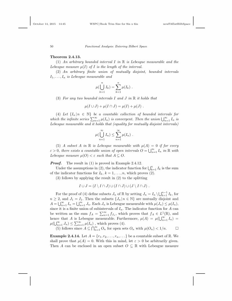
October 14, 2015 14:45 WSPC/Book Trim Size for 9in x 6in newFAEntHilbSpace
50 Functional Analysis: Entering Hilbert Space
Theorem 2.4.13.
(1) An arbitrary bounded interval I in R is Lebesgue measurable and the
Lebesgue measure µ(I) of I is the length of the interval.
(2) An arbitrary finite union of mutually disjoint, bounded intervals
I1, . . . , In is Lebesgue measurable and
µ(
n⋃
k=1
Ik) =
n∑
k=1
µ(Ik) .
(3) For any two bounded intervals I and J in R it holds that
µ(I ∪ J) + µ(I ∩ J) = µ(I) + µ(J) .
(4) Let {In |n ∈ N} be a countable collection of bounded intervals for
which the infinite series∑∞
n=1 µ(In) is convergent. Then the union⋃∞
n=1 In is
Lebesgue measurable and it holds that (equality for mutually disjoint intervals)
µ(
∞⋃
n=1
In) ≤∞∑
n=1
µ(In) .
(5) A subset A in R is Lebesgue measurable with µ(A) = 0 if for every
ε > 0, there exists a countable union of open intervals O =⋃∞
n=1 In in R with
Lebesgue measure µ(O) < ε such that A ⊆ O.
Proof. The result in (1) is proved in Example 2.4.12.
Under the assumptions in (2), the indicator function for⋃n
k=1 Ik is the sum
of the indicator functions for Ik, k = 1, . . . , n, which proves (2).
(3) follows by applying the result in (2) to the splitting
I ∪ J = (I \ I ∩ J) ∪ (I ∩ J) ∪ (J \ I ∩ J) .
For the proof of (4) define subsets Jn of R by setting Jn = In \⋃n−1
k=1 Ik, for
n ≥ 2, and J1 = I1. Then the subsets {Jn |n ∈ N} are mutually disjoint and
A =⋃∞
n=1 In =⋃∞
n=1 Jn. Each Jn is Lebesgue measurable with µ(Jn) ≤ µ(In),
since it is a finite union of subintervals of In. The indicator function for A can
be written as the sum fA =∑∞
n=1 fJn, which proves that fA ∈ L1(R), and
hence that A is Lebesgue measurable. Furthermore, µ(A) = µ(⋃∞
n=1 In) =
µ(⋃∞
n=1 Jn) ≤∑∞
n=1 µ(In) , which proves (4).
(5) follows since A ⊆ ⋂∞n=1On for open sets On with µ(On) < 1/n. �
Example 2.4.14. Let A = {r1, r2, . . . , rn, . . . } be a countable subset of R. We
shall prove that µ(A) = 0. With this in mind, let ε > 0 be arbitrarily given.
Then A can be enclosed in an open subset O ⊆ R with Lebesgue measure

October 14, 2015 14:45 WSPC/Book Trim Size for 9in x 6in newFAEntHilbSpace
Chapter 2: New Types of Function Spaces 51
µ(O) < ε by choosing an open interval In of length ε/2n containing rn for all
n ∈ N and letting O =⋃∞
n=1 In. By property (5) in Theorem 2.4.13 it follows
that A is Lebesgue measurable with µ(A) = 0.
Example 2.4.15. We shall construct the Cantor set C, introduced by and
named after the German mathematician Georg Cantor (1845–1918).
In the first step of the construction, we subdivide the unit interval [0, 1]
into three subintervals of equal lengths and then exclude the open middle
interval (13 ,23 ). In the second step, we divide each of the two intervals [0, 13 ]
and [ 23 , 1] into three equal parts and exclude (19 ,29 ), respectively (79 ,
89 ), from
those. Continue this way ad infinitum, in step n dividing each of the remaining
closed intervals from step n− 1 into three equal parts and excluding the open
middle intervals. In the limit we get the Cantor set C.
We can view C as the complement C = [0, 1] \ S, where S is the union of
the recursively defined open sets,
S1 =(13,2
3
)
S2 =(19,2
9
)∪(79,8
9
)
S3 =( 1
27,2
27
)∪( 7
27,8
27
)∪(1927,20
27
)∪(2527,26
27
)
...
Arguing as in Example 2.4.12, it can be proved that S is Lebesgue measur-
able and with Lebesgue measure,
µ(S) =
∫ 1
0
fS(x)dx =
∫ 1
0
1dx = 1 .
Since fC = 1 − fS , it follows that fC ∈ L1(R), and hence that the Cantor
set C is Lebesgue measurable. We also get that the Cantor set has Lebesgue
measure 0, since
µ(C) =
∫
R
fC(x)dx =
∫ 1
0
(1− fS(x))dx = 1− 1 = 0 .
If we write the numbers in [0, 1] as power series∑∞
1 an(1/3)n, with an =
0, 1, 2 (triadic expansion), then the numbers in C are represented by triadic
expansions with coefficients an either 0 or 2. We can then prove that the set
C is uncountable by an indirect argument. For suppose r1, r2, . . . , rn, . . . is
the complete list of numbers in C. Then construct a number r with triadic
expansion r =∑∞
1 an(1/3)n by choosing the coefficient an to be either 0 or

October 14, 2015 14:45 WSPC/Book Trim Size for 9in x 6in newFAEntHilbSpace
52 Functional Analysis: Entering Hilbert Space
2 but different from the nth coefficient in rn for each n ∈ N. Now r is a
new number in C contradicting that r1, r2, . . . , rn, . . . is the complete list of
numbers in C.
The Cantor set C provides an example of an uncountable subset of [0, 1]
with Lebesgue measure 0, thus proving that Lebesgue measure 0 is not re-
stricted to countable sets as in Example 2.4.14.
2.4.3 Smooth functions with compact support
There are other nice subspaces that are dense in the Lp-spaces than the space
C0(R) of continuous functions with compact support.
Definition 2.4.16. Denote by C∞0 (R) the set of functions f : R → C that are
infinitely often differentiable (smooth) and have compact support.
Example 2.4.17. One may wonder if such functions do exist. Here is one with
compact support in the closed and bounded interval [a, b]:
ϕa,b(x) =
{exp
(−1
(x−a)(b−x)
)for x ∈ ]a, b[
0 otherwise.
Differentiability at x = a and x = b is ensured by the fact that exponential
functions grow faster than polynomial functions. For good reasons, the function
ϕa,b is called a bump function.
x
y
ba
Fig. 2.3 Graph of ϕa,b
We state the following useful result without proof.

October 14, 2015 14:45 WSPC/Book Trim Size for 9in x 6in newFAEntHilbSpace
Chapter 2: New Types of Function Spaces 53
Theorem 2.4.18.
(1) The space C∞0 (R) is dense in C0(R) both with respect to the uniform
norm (supremum norm) and to the p-norm, p ≥ 1.
(2) The space C∞0 (R) is dense in all the spaces Lp(R), p ≥ 1.
2.4.4 Riemann integrable functions
The space of Riemann integrable functions is the classical space of func-
tions considered in connection with integration theory. In this section we shall
demonstrate that the space of absolute pth power Riemann integrable functions
can be identified with a dense subspace of the corresponding Lp-space.
First we recall the definition of Riemann integrability.
Let f : [a, b] → C be a bounded function defined in a closed and bounded
interval [a, b] in R. For any partition D of the interval [a, b] into a finite number
of subintervals [ti−1, ti], 1 ≤ i ≤ n, marked by the points
D : a = t0 < t1 < · · · < tn−1 < tn = b ,
and for any selection τ1, τ2, . . . , τn of points in [a, b] such that τi ∈ [ti−1, ti] for
1 ≤ i ≤ n, define the Riemann sum
S(f,D) =
n∑
i=1
f(τi)(ti − ti−1) .
The norm of the partition is the number
µ(D) = max{| ti − ti−1 |
∣∣ i = 1, . . . , n}.
The function f : [a, b] → C is said to be Riemann integrable if the collection
of Riemann sums S(f,D) has a limit for µ(D) → 0. In case of integrability,
the limit is called the Riemann integral of f and it is denoted by∫ b
a f(x)dx. In
short, the Riemann integral is given by
∫ b
a
f(x)dx = limµ(D)→0
S(f,D) .
Now consider a bounded function f : R → C with compact support. By
choosing a closed and bounded interval containing the support of f we can
define the notion of Riemann integrability also for such functions. Let R0(R)
denote the space of bounded, Riemann integrable functions with compact sup-
port. We can introduce a vector space structure in R0(R) by the obvious point-
wise defined operations. Then C0(R) is a linear subspace in R0(R).

October 14, 2015 14:45 WSPC/Book Trim Size for 9in x 6in newFAEntHilbSpace
54 Functional Analysis: Entering Hilbert Space
For any real number p ≥ 1, a bounded function f : R → C with compact
support is said to be absolute pth power Riemann integrable if the following
integral exists in the sense of Riemann,∫
R
|f(x) |pdx .
Denote by Rp0(R) the space of all such functions.
For every function f ∈ Rp0(R), we can define the p-norm
||f ||p =( ∫
R
|f(x) |pdx)1/p
.
The inequalities of Holder, Cauchy-Schwarz and Minkowski can be proved
for the spaces Rp0(R) by limit arguments with Riemann sums. In particular,
we get the (semi) normed vector space (Rp0(R), || · ||p) containing the normed
vector space (C0(R), || · ||p) as a dense subspace.
Remark 2.4.19. The p-norm || · ||p is only a so-called seminorm in Rp0(R) since
it can happen that ||f ||p = 0 for a nonzero f ∈ Rp0(R). This will be of no
importance for the validity of the proof of Theorem 2.4.20.
The pth power Riemann integrable functions with compact support can be
considered as Lp-functions. This is the message of the following theorem.
Theorem 2.4.20. For any p ≥ 1, the space (Rp0(R), || · ||p) can be identified
with a dense subspace in (Lp(R), || · ||p). With this identification, we have the
linear and isometric (with respect to p-norm) inclusions
C0(R) ⊂ Rp0(R) ⊂ Lp(R)
and
C0(R) = Rp0(R) = Lp(R) .
Proof. The only thing to be proved is that a Cauchy sequence in
(Rp0(R), || · ||p) is equivalent to a Cauchy sequence in (C0(R), || · ||p). This follows
by observing that if (fn) is a Cauchy sequence in (Rp0(R), || · ||p), then we can
construct a Cauchy sequence (gn) in (C0(R), || · ||p) such that ||fn − gn ||p → 0
for n→ ∞. This is left to the reader as an exercise. �
We finish this section by stating (without proof) a result that characterizes
the Riemann integrable functions among the Lebesgue integrable functions.
Theorem 2.4.21. Let f : [a, b] → R be a bounded, real-valued function defined
in the closed and bounded interval [a, b]. Suppose that f is Lebesgue integrable,

October 14, 2015 14:45 WSPC/Book Trim Size for 9in x 6in newFAEntHilbSpace
Chapter 2: New Types of Function Spaces 55
i.e. f ∈ L1([a, b]). Then f : [a, b] → R is a Riemann integrable function if and
only if the set of points where f is not continuous is contained in a set of
Lebesgue measure zero.
Example 2.4.22. Let A be the subset of rational numbers in the closed unit
interval [0, 1] and let fA : [0, 1] → R be the indicator function for A. Since the
set of rational numbers is countable, the function fA is Lebesgue integrable
with Lebesgue integral ||fA ||1 =∫ 1
0fA(x)dx = 0.
On the other hand, the function fA is not Riemann integrable since its
Riemann sums fluctuate between 0 and 1. Note that there is no conflict with
Theorem 2.4.21, even though the Lebesgue measure µ(A) = 0, since fA is not
continuous at any point of [0, 1].
2.5 The sequence spaces lp
Corresponding to the function spaces Lp(R), there are similar notions for spaces
of sequences (xn) in R (or C).
This is not surprising since a sequence (xn) can actually be viewed as a
function f : N → R (or C) by the identification xn = f(n), n ∈ N. To transfer
results from the continuous case to the discrete case, we just have to substitute∫Rdx by
∑∞n=1; for example
∫R|f(x) |pdx should be substituted by
∑∞n=1 |xn |p.
This leads to the so-called lp-spaces, p ≥ 1.
Definition 2.5.1. For any real number p ≥ 1, a (real or complex) sequence
(xn) is said to be absolute p-summable, if the infinite series of pth-powers of
absolute values of the elements in the sequence is convergent, i.e.
∞∑
n=1
|xn |p <∞ .
(i) Denote by lp, p ≥ 1, the space of all absolute p-summable sequences.
The norm in lp is defined by
||(xn) ||p =( ∞∑
n=1
|xn |p)1/p
.
(ii) Denote by l∞ the sequence space of all bounded sequences (xn). The
norm in l∞ is defined by
||(xn) ||∞ = supn∈N
|xn | .

October 14, 2015 14:45 WSPC/Book Trim Size for 9in x 6in newFAEntHilbSpace
56 Functional Analysis: Entering Hilbert Space
To justify the terminology used in Definition 2.5.1, we need to prove that
lp is indeed a normed vector space with the norm || · ||p. This will follow by
Minkowski’s inequality for sequences, which we shall prove below.
First we prove Holder’s inequality for sequences.
Theorem 2.5.2 (Holder’s inequality). Let p > 1, q > 1 be a pair of real
numbers satisfying 1/p+1/q = 1. For any pair of sequences (xn) ∈ lp, (yn) ∈ lq,
the product sequence (xnyn) ∈ l1, and the following inequality holds
||(xnyn) ||1 ≤ ||(xn) ||p||(yn) ||q .
In detail:∞∑
n=1
|xnyn | ≤( ∞∑
n=1
|xn |p)1/p( ∞∑
n=1
|yn |q)1/q
.
Proof. The inequality is clearly satisfied if either (xn) or (yn) is the constant
sequence with all elements 0. Hence we can assume that ||(xn) ||p > 0 and
||(yn) ||q > 0.
By Young’s inequality, Theorem 2.3.5, we first get,
|xnyn |||(xn) ||p ||(yn) ||q
=|xn |
||(xn) ||p|yn |
||(yn) ||q≤ 1
p
|xn |p||(xn) ||pp
+1
q
|yn |q||(yn) ||qq
,
and then by summation,
N∑
n=1
|xnyn |||(xn) ||p ||(yn) ||q
≤ 1
p
N∑
n=1
|xn |p||(xn) ||pp
+1
q
N∑
n=1
|yn |q||(yn) ||qq
≤ 1
p
||(xn) ||pp||(xn) ||pp
+1
q
||(yn) ||qq||(yn) ||qq
=1
p+
1
q= 1 ,
from which follows that ||(xnyn) ||1 ≤ ||(xn) ||p||(yn) ||q by letting N → ∞. �
As a special case, we get Cauchy-Schwarz’ inequality.
Corollary 2.5.3 (Cauchy-Schwarz’ inequality). For any pair of square-
summable sequences (xn), (yn) ∈ l2, the product sequence (xnyn) ∈ l1, and
the following inequality holds
||(xnyn) ||1 ≤ ||(xn) ||2||(yn) ||2 .
In detail:∞∑
n=1
|xnyn | ≤( ∞∑
n=1
|xn |2)1/2( ∞∑
n=1
|yn |2)1/2
.

October 14, 2015 14:45 WSPC/Book Trim Size for 9in x 6in newFAEntHilbSpace
Chapter 2: New Types of Function Spaces 57
As the following theorem will show, the sum of two sequences in lp is again
a sequence in lp, thereby proving (the difficult part of the argument) that lp
is a vector space. Furthermore, the inequality in the theorem is exactly the
triangle inequality for || · ||p.
Theorem 2.5.4 (Minkowski’s inequality). For any real number p ≥ 1, and
any pair of p-summable sequences (xn), (yn) ∈ lp, the sum sequence (xn + yn)
is p-summable, i.e. (xn + yn) ∈ lp, and the following inequality holds
||(xn + yn) ||p ≤ ||(xn) ||p + ||(yn) ||p .
In detail:
( ∞∑
n=1
|xn + yn |p)1/p
≤( ∞∑
n=1
|xn |p)1/p
+( ∞∑
n=1
|yn |p)1/p
.
Proof. For p = 1, the proof follows by using the triangle inequality for the
numerical value to obtain the estimates
N∑
n=1
|xn + yn | ≤N∑
n=1
|xn |+N∑
n=1
|yn | ≤∞∑
n=1
|xn |+∞∑
n=1
|yn | ,
and then letting N → ∞.
For p > 1, put 1/q = 1− 1/p. Then we have a pair of real numbers p > 1,
q > 1, satisfying 1/p+ 1/q = 1.
First an elementary rewriting,
SN =
N∑
n=1
|xn + yn |p =
N∑
n=1
|xn + yn | |xn + yn |p−1 .
Applying the triangle inequality for the numerical value, we then get
SN ≤N∑
n=1
|xn | |xn + yn |p−1 +
N∑
n=1
|yn | |xn + yn |p−1 .
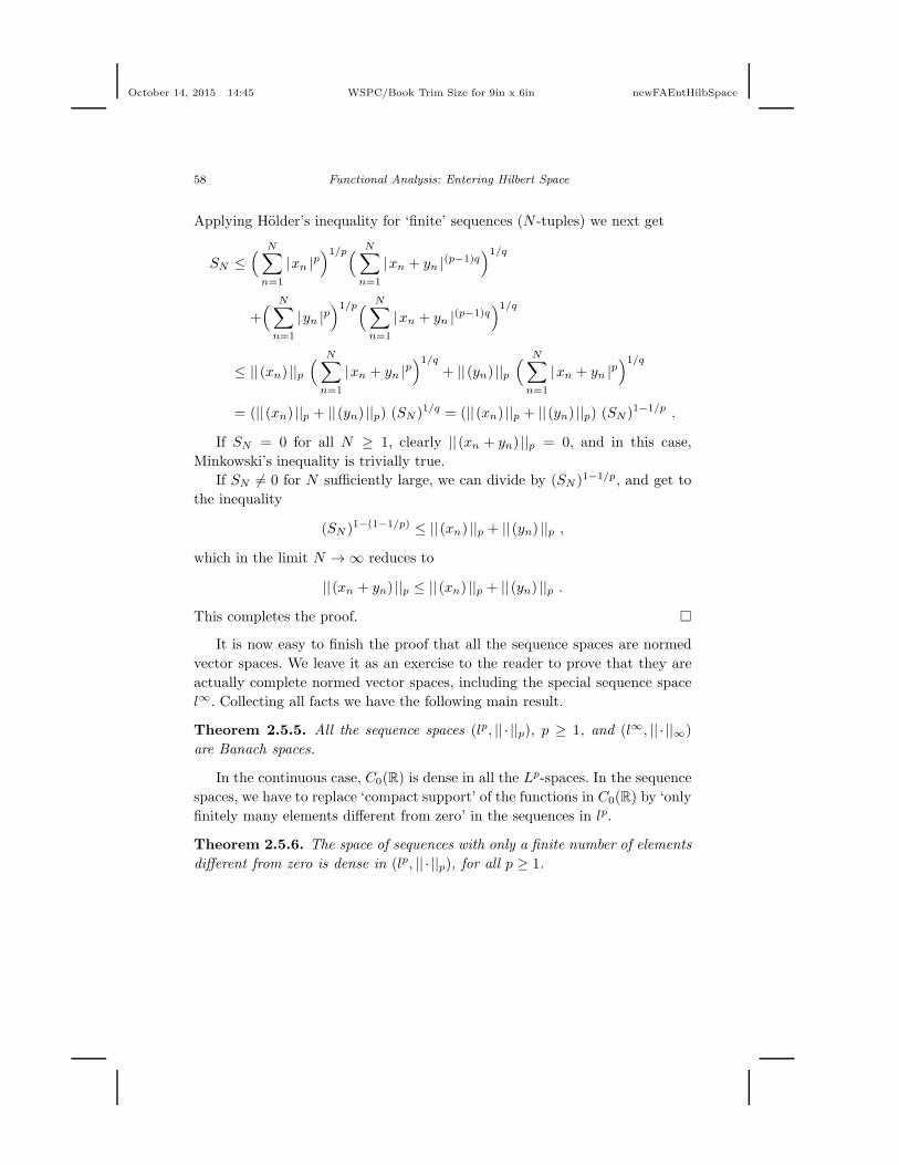
October 14, 2015 14:45 WSPC/Book Trim Size for 9in x 6in newFAEntHilbSpace
58 Functional Analysis: Entering Hilbert Space
Applying Holder’s inequality for ‘finite’ sequences (N -tuples) we next get
SN ≤( N∑
n=1
|xn |p)1/p( N∑
n=1
|xn + yn |(p−1)q)1/q
+( N∑
n=1
|yn |p)1/p( N∑
n=1
|xn + yn |(p−1)q)1/q
≤ ||(xn) ||p( N∑
n=1
|xn + yn |p)1/q
+ ||(yn) ||p( N∑
n=1
|xn + yn |p)1/q
= (||(xn) ||p + ||(yn) ||p) (SN )1/q = (||(xn) ||p + ||(yn) ||p) (SN )1−1/p .
If SN = 0 for all N ≥ 1, clearly ||(xn + yn) ||p = 0, and in this case,
Minkowski’s inequality is trivially true.
If SN 6= 0 for N sufficiently large, we can divide by (SN )1−1/p, and get to
the inequality
(SN )1−(1−1/p) ≤ ||(xn) ||p + ||(yn) ||p ,
which in the limit N → ∞ reduces to
||(xn + yn) ||p ≤ ||(xn) ||p + ||(yn) ||p .
This completes the proof. �
It is now easy to finish the proof that all the sequence spaces are normed
vector spaces. We leave it as an exercise to the reader to prove that they are
actually complete normed vector spaces, including the special sequence space
l∞. Collecting all facts we have the following main result.
Theorem 2.5.5. All the sequence spaces (lp, || · ||p), p ≥ 1, and (l∞, || · ||∞)
are Banach spaces.
In the continuous case, C0(R) is dense in all the Lp-spaces. In the sequence
spaces, we have to replace ‘compact support’ of the functions in C0(R) by ‘only
finitely many elements different from zero’ in the sequences in lp.
Theorem 2.5.6. The space of sequences with only a finite number of elements
different from zero is dense in (lp, || · ||p), for all p ≥ 1.
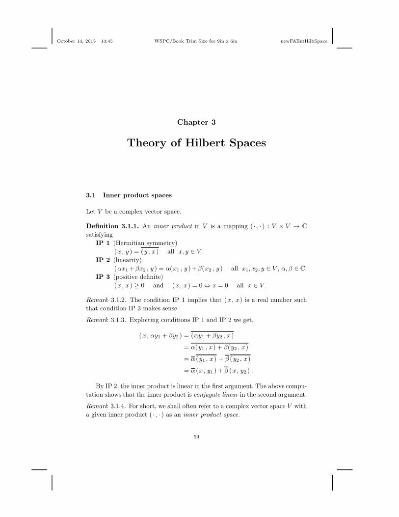
October 14, 2015 14:45 WSPC/Book Trim Size for 9in x 6in newFAEntHilbSpace
Chapter 3
Theory of Hilbert Spaces
3.1 Inner product spaces
Let V be a complex vector space.
Definition 3.1.1. An inner product in V is a mapping ( · , ·) : V × V → C
satisfying
IP 1 (Hermitian symmetry)
(x, y ) = (y , x) all x, y ∈ V .
IP 2 (linearity)
(αx1 +βx2 , y ) = α(x1 , y )+β(x2 , y ) all x1, x2, y ∈ V , α, β ∈ C.
IP 3 (positive definite)
(x, x) ≥ 0 and (x, x) = 0 ⇔ x = 0 all x ∈ V .
Remark 3.1.2. The condition IP 1 implies that (x, x) is a real number such
that condition IP 3 makes sense.
Remark 3.1.3. Exploiting conditions IP 1 and IP 2 we get,
(x, αy1 + βy2 ) = (αy1 + βy2 , x)
= α(y1 , x) + β(y2 , x)
= α (y1 , x) + β (y2 , x)
= α (x, y1 ) + β (x, y2 ) .
By IP 2, the inner product is linear in the first argument. The above compu-
tation shows that the inner product is conjugate linear in the second argument.
Remark 3.1.4. For short, we shall often refer to a complex vector space V with
a given inner product ( · , ·) as an inner product space.
59
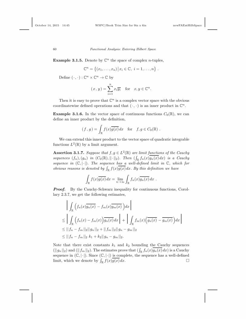
October 14, 2015 14:45 WSPC/Book Trim Size for 9in x 6in newFAEntHilbSpace
60 Functional Analysis: Entering Hilbert Space
Example 3.1.5. Denote by Cn the space of complex n-tuples,
Cn ={(x1, . . . , xn)
∣∣xi ∈ C, i = 1, . . . , n}.
Define ( · , ·) : Cn × Cn → C by
(x, y ) =n∑
i=1
xiyi for x, y ∈ Cn.
Then it is easy to prove that Cn is a complex vector space with the obvious
coordinatewise defined operations and that ( · , ·) is an inner product in Cn.
Example 3.1.6. In the vector space of continuous functions C0(R), we can
define an inner product by the definition,
(f , g ) =
∫
R
f(x)g(x)dx for f, g ∈ C0(R) .
We can extend this inner product to the vector space of quadratic integrable
functions L2(R) by a limit argument.
Assertion 3.1.7. Suppose that f, g ∈ L2(R) are limit functions of the Cauchy
sequences (fn), (gn) in (C0(R), || · ||2). Then (∫Rfn(x)gn(x)dx) is a Cauchy
sequence in (C, | · |). The sequence has a well-defined limit in C, which for
obvious reasons is denoted by∫Rf(x)g(x)dx. By this definition we have
∫
R
f(x)g(x)dx = limn→∞
∫
R
fn(x)gn(x)dx .
Proof. By the Cauchy-Schwarz inequality for continuous functions, Corol-
lary 2.3.7, we get the following estimates,
|∫R
(fn(x)gn(x) − fm(x)gm(x)
)dx|
≤|∫R
(fn(x)− fm(x)
)gn(x)dx|+ |∫
R
fm(x)(gn(x) − gm(x)
)dx|
≤ ||fn − fm ||2||gn ||2 + ||fm ||2||gn − gm ||2≤ ||fn − fm ||2 k1 + k2||gn − gm ||2.
Note that there exist constants k1 and k2 bounding the Cauchy sequences
(||gn ||2) and (||fm ||2). The estimates prove that (∫Rfn(x)gn(x)dx) is a Cauchy
sequence in (C, | · |). Since (C, | · |) is complete, the sequence has a well-defined
limit, which we denote by∫Rf(x)g(x)dx. �

October 14, 2015 14:45 WSPC/Book Trim Size for 9in x 6in newFAEntHilbSpace
Chapter 3: Theory of Hilbert Spaces 61
We can now immediately extend the inner product in C0(R) to L2(R) by
the definition
(f , g ) =
∫
R
f(x)g(x)dx for f, g ∈ L2(R) .
The norm || · ||2 in L2(R) is given by
||f ||2 = (∫
R
|f(x) |2dx)1/2
= (∫
R
f(x)f(x)dx)1/2
=√(f , f ) .
Unless otherwise specified, we shall always assume that L2(R) is equipped
with the above inner product ( · , ·) and the related norm || · ||2.
Lemma 3.1.8. Let ( · , ·) be an inner product in the complex vector space V .
Then we have the following inequality
|(x, y ) |2 ≤ (x, x)(y , y ) for all x, y ∈ V .
Proof. If (y , y ) = 0, then y = 0, and the inequality is trivially true. Suppose
therefore that (y , y ) 6= 0.
For any α ∈ C we get
0 ≤ (x− αy , x− αy ) = (x, x)− α(y , x)− α (x, y ) + αα (y , y ) .
Put α = (x, y )/(y , y ) and we get
0 ≤ (x, x) − (x, y )
(y , y )(y , x)− (x, y )
(y , y )(x, y ) +
(x, y )
(y , y )
(x, y )
(y , y )(y , y )
= (x, x) − (x, y )(x, y )
(y , y ).
The inequality now follows immediately. �
In Example 3.1.6 it was shown how the 2-norm || · ||2 in L2(R) can be derived
from the inner product ( · , ·) in L2(R). A similar construction can be applied
to derive a norm from an inner product in an arbitrary vector space.
Theorem 3.1.9. Let V be a complex vector space with an inner product ( · , ·).Then the inner product induces a norm || · || in V by the definition
||x || =√(x, x) for x ∈ V .

October 14, 2015 14:45 WSPC/Book Trim Size for 9in x 6in newFAEntHilbSpace
62 Functional Analysis: Entering Hilbert Space
Proof. We have to prove that || · || satisfies the three conditions for a norm.
NORM 1 follows by IP 3:
||x || =√(x, x) ≥ 0, = 0 ⇔ x = 0 ,
for all x ∈ V .
NORM 2 follows by using the linearity properties of the inner product:
||αx || =√(αx, αx) =
√αα (x, x) =
√|α |2(x, x) = |α |||x || ,
for all α ∈ C, and all x ∈ V .
NORM 3, the triangle inequality, follows by a computation using in turn
the linearity properties of the inner product, IP 1, and Lemma 3.1.8:
||x + y ||2 = (x+ y , x+ y )
= ||x ||2 + ||y ||2 + (x, y ) + (y , x)
= ||x ||2 + ||y ||2 + (x, y ) + (x, y )
= ||x ||2 + ||y ||2 + 2Re[(x, y )]
≤ ||x ||2 + ||y ||2 + 2 |(x, y ) |≤ ||x ||2 + ||y ||2 + 2 ||x || ||y ||=
(||x ||+ ||y ||
)2,
for all x, y ∈ V . �
Remark 3.1.10. The norm || · || defined by the procedure in Theorem 3.1.9 is
called the induced norm given by the inner product ( · , ·).Having proved that the construction in Theorem 3.1.9 actually defines a
norm, Lemma 3.1.8 can be reformulated as Cauchy-Schwarz’ inequality for a
general vector space with an inner product.
Theorem 3.1.11 (Cauchy-Schwarz’ inequality). Let V be a complex vector
space with an inner product ( · , ·) and induced norm || · ||. Then we have the
inequality
|(x, y ) | ≤ ||x || ||y || for all x, y ∈ V .
The inner product is continuous in both variables. This is the message in
the following result.
Proposition 3.1.12. Let ( · , ·) be an inner product in the complex vector space
V and let || · || be the induced norm.

October 14, 2015 14:45 WSPC/Book Trim Size for 9in x 6in newFAEntHilbSpace
Chapter 3: Theory of Hilbert Spaces 63
If the sequences (xn) and (yn) in V are convergent to x ∈ V , respectively
y ∈ V , then the sequence of inner products ((xn , yn )) converges to (x, y ), i.e.
xn → x
yn → y
}for n→ ∞ =⇒ (xn , yn ) → (x, y ) for n→ ∞ .
Proof. First observe that
(xn , yn )− (x, y ) = (xn , yn )− (x, yn ) + (x, yn )− (x, y )
= (xn − x, yn ) + (x, yn − y )
= (xn − x, yn − y ) + (xn − x, y ) + (x, yn − y ) .
From this we get by the Cauchy-Schwarz inequality:
|(xn , yn )− (x, y ) | = |(xn − x, yn − y ) + (xn − x, y ) + (x, yn − y ) |≤ |(xn − x, yn − y ) |+ |(xn − x, y ) |+ |(x, yn − y ) |≤ ||xn − x || ||yn − y ||+ ||xn − x || ||y ||+ ||x || ||yn − y || .
The proposition now follows easily. �
xy
(x,y)v
Fig. 3.1 Inner product of vectors in R3
In 3-dimensional Euclidean space R3 with the canonical inner product
(x, y ) =∑3
i=1 xiyi, it is well known that two vectors x, y ∈ R3 are orthogo-
nal in the usual geometrical sense of the word, written x ⊥ y, if and only if
(x, y ) = 0. This follows from the alternative formula for the inner product of
two vectors x, y ∈ R3 forming an angle of v:
(x, y ) = ||x || ||y || cos v .
Up to sign, the inner product (x, y ) of vectors x, y ∈ R3 is the length of the
orthogonal projection of y onto x multiplied by the length of x; cf. Figure 3.1.

October 14, 2015 14:45 WSPC/Book Trim Size for 9in x 6in newFAEntHilbSpace
64 Functional Analysis: Entering Hilbert Space
We use the 3-dimensional Euclidean case to motivate the definition of or-
thogonality of vectors in arbitrary inner product spaces.
Definition 3.1.13. In a complex vector space V with inner product ( · , ·),two vectors x, y ∈ V are said to be orthogonal, written x ⊥ y, if (x, y ) = 0.
For orthogonal vectors we have an abstract version of Pythagoras’ theorem.
Theorem 3.1.14 (Pythagoras’ theorem). Suppose that x and y is an arbitrary
pair of orthogonal vectors in the inner product space V , i.e. suppose x ⊥ y.
Then we have Pythagoras’ formula
||x+ y ||2 = ||x ||2 + ||y ||2 .
Proof. The proof follows by the easy computation
||x+ y ||2 = (x+ y , x+ y ) = ||x ||2 + ||y ||2 +(x, y )+ (y , x) = ||x ||2+ ||y ||2 ,
since (x, y ) = (y , x) = 0. �
3.2 Hilbert spaces
Let V be a complex vector space with an inner product ( · , ·) and the induced
norm || · ||. If V is a Banach space, in other words a complete normed vector
space, with respect to the induced norm || · ||, it is called a Hilbert space.
Definition 3.2.1. A Hilbert space is an inner product space V which is a
Banach space with respect to the induced norm.
Example 3.2.2. Here are some main examples of Hilbert spaces.
1. Cn with the standard inner product is a Hilbert space. It boils down to
the fact that R2n with Euclidean norm is a complete space.
2. L2(R) with the inner product
(f , g ) =
∫
R
f(x)g(x)dx ,
inducing the 2-norm || · ||2, is by construction a complete space and hence a
Hilbert space.
3. l2, the space of square summable complex sequences (xn), i.e. sequences
for which∑∞
n=1 |xn |2 <∞, is a Hilbert space with the inner product
((xn) , (yn)) =
∞∑
n=1
xnyn .

October 14, 2015 14:45 WSPC/Book Trim Size for 9in x 6in newFAEntHilbSpace
Chapter 3: Theory of Hilbert Spaces 65
Note that the series∑∞
n=1 xnyn is convergent, so that the inner product is
defined. This is an immediate consequence of the Cauchy-Schwarz inequality:
∞∑
n=1
|xnyn | ≤ ||(xn) ||2||(yn) ||2 .
The properties required for an inner product are easily established. And so is
completeness of the space.
3.3 Basis in a normed vector space and separability
Several constructions in functional analysis involve objects defined as sums of
infinite series in normed vector spaces. Fortunately the basic theory of such in-
finite series is completely parallel to the theory of series with complex numbers
as terms.
3.3.1 Infinite series in normed vector spaces
Let V be a normed vector space with norm || · ||.By a series
∑∞n=1 xn in V , we understand a sequence x1, x2, . . . , xn, . . . of
elements of V which we, to begin with, just formally sum. To the series there
corresponds a sequence of partial sums s1, s2, . . . , sn, . . . defined by
sn =
n∑
k=1
xk = x1 + · · ·+ xn.
We say that the series is convergent with sum s ∈ V if the sequence of partial
sums (sn) is convergent with limit point s. In case of convergence we write
s =
∞∑
n=1
xn.
The nth term xn in a series∑∞
n=1 xn can be written in the form xn = sn−sn−1,
which gives the following necessary condition for convergence of a series.
Theorem 3.3.1. In a convergent series∑∞
n=1 xn in the normed vector space
V , the nth term xn converges to 0 ∈ V for n going to ∞.
Since a Banach space considered as a metric space is complete, we also have
the following important result.

October 14, 2015 14:45 WSPC/Book Trim Size for 9in x 6in newFAEntHilbSpace
66 Functional Analysis: Entering Hilbert Space
Theorem 3.3.2 (The Cauchy condition for series). A series∑∞
n=1 xn in a
Banach space V is convergent if and only if
∀ε > 0 ∃n0 ∈ N ∀n, k ∈ N : n ≥ n0 ⇒ ||sn+k − sn || < ε,
or equivalently,
∀ε > 0 ∃n0 ∈ N ∀n, k ∈ N : n ≥ n0 ⇒ ||n+k∑
i=n+1
xi || < ε.
From the Cauchy condition we deduce a very useful test for convergence.
Theorem 3.3.3 (The comparison test). Let∑∞
n=1 xn be a series in a Ba-
nach space V . If there exists a convergent series of non-negative real numbers∑∞n=1 an such that ||xn || ≤ an for n ≥ n0 from a certain step n0, then the
series∑∞
n=1 xn is convergent.
Proof. For n ≥ n0, the triangle inequality gives the inequality
||n+k∑
i=n+1
xi || ≤n+k∑
i=n+1
ai.
Since the Cauchy condition is satisfied in both V and R, the result follows
immediately. �
A series∑∞
n=1 xn is said to be divergent, if it is not convergent.
3.3.2 Separability of a normed vector space
Let V be a normed vector space with norm || · ||.If there exists a finite set {x1, . . . , xn} of elements in V with the property
that every element x ∈ V can be written in a unique manner as a linear
combination,
x = α1x1 + · · ·+ αnxn , αi ∈ C ,
then it is well known from basic linear algebra that the number n is uniquely
determined. We say that V is finite dimensional of dimension n and that
{x1, . . . , xn} is a basis for V .
If there exists a countable set {x1, . . . , xn, . . . } of elements in V , in other
words a sequence (xn) in V , then we say that the sequence (xn) is a Schauder
basis in V , if every element x ∈ V admits a unique decomposition as the sum

October 14, 2015 14:45 WSPC/Book Trim Size for 9in x 6in newFAEntHilbSpace
Chapter 3: Theory of Hilbert Spaces 67
of a convergent series
x =
∞∑
n=1
αnxn , αn ∈ C, ∀n ∈ N .
If (xn) is a Schauder basis in V it follows in particular that
x =
∞∑
n=1
αnxn = 0 ⇐⇒ αn = 0, ∀n ∈ N .
This implies that every finite subset of elements in the basis (xn) is a linearly
independent set of elements in V . Hence a normed vector space V with a
Schauder basis is necessarily of infinite dimension since it contains subspaces
of an arbitrary finite dimension.
Definition 3.3.4. We call a normed vector space V separable by a basis if V
admits a finite basis (finite dimension) or a Schauder basis (infinite dimension).
For topological spaces, there is a more general notion of separability.
Definition 3.3.5. A topological space S is called separable if it admits a
countable dense subset W .
Definition 3.3.5 applies in particular to metric spaces and hence also to
normed vector spaces. For normed vector spaces we then have two notions
of separability. As the following theorem shows, separability by a basis is a
stronger notion than just separability.
Theorem 3.3.6. If a normed vector space V is separable by a basis, then it
is separable.
Proof. If V is a finite dimensional normed vector space, we consider the set
of points W in V defined by all linear combinations of a finite set of basis
vectors for V , using only such complex numbers as coefficients for which both
the real part and the imaginary part are rational numbers. This set of points
W is countable, since the set of rational numbers is countable. The set W is
furthermore dense in V , since the set of rational numbers is dense in the set
of real numbers.
If V admits a Schauder basis, we consider by analogy the set of points W
in V defined by all finite linear combinations of the set of vectors in a Schauder
basis for V , using only such complex numbers as coefficients for which both
the real part and the imaginary part are rational numbers. Also in this case,
the set of points W is countable and dense in V . This completes the proof. �

October 14, 2015 14:45 WSPC/Book Trim Size for 9in x 6in newFAEntHilbSpace
68 Functional Analysis: Entering Hilbert Space
Remark 3.3.7. In the case of Hilbert spaces, separability by a basis coincides
with the general notion of separability; cf. Theorem 3.3.6 and Theorem 3.4.9.
For Banach spaces, the two notions of separability do not agree. After it had
been an open problem for 40 years, the Swedish mathematician Per Enflo in
1973 gave examples of Banach spaces that contain a countable dense subset
of points but do not admit a Schauder basis. In this context, further remark-
able new discoveries about Banach spaces were made towards the end of the
20th century by the British mathematician William Timothy Gowers, who was
awarded a Fields medal for his work in 1998.
All normed vector spaces considered in this book will in practice be finite
dimensional, or, at least separable, infinite dimensional. This will be sufficient
to cover most applications.
Example 3.3.8. Let l2 be the space of square summable sequences. Then l2
is an infinite dimensional, separable Hilbert space, and the sequence (en) in
l2, where en = (. . . , 1, . . . ) is the sequence in C with 1 at the nth place and 0
otherwise, is a Schauder basis for l2.
3.4 Basis in a separable Hilbert space
The basis (en) in l2 in Example 3.3.8 is of a particular convenient type. It is
an orthonormal basis.
Definition 3.4.1. A set of vectors {xk} in an inner product space is called
an orthogonal set if (xi , xj ) = 0 for i 6= j, and xj 6= 0 for all j. If furthermore
(xj , xj ) = 1 for all j, in other words, if all the vectors are unit vectors, then
the set is called an orthonormal set. A sequence (xn), which as a set {xn} is
orthonormal, is called an orthonormal sequence.
If an orthonormal set of vectors in an inner product space is a basis for
the vector space, then we call the set an orthonormal basis - a terminology
that applies both in the finite dimensional case and in the separable, infinite
dimensional case.
Proposition 3.4.2. An arbitrary finite orthogonal set in an inner product
space is linearly independent.
Proof. Suppose that {e1, . . . , en} is an orthogonal set in an inner product
space and that we are given a vanishing linear combination
α1e1 + · · ·+ αnen = 0 .

October 14, 2015 14:45 WSPC/Book Trim Size for 9in x 6in newFAEntHilbSpace
Chapter 3: Theory of Hilbert Spaces 69
Then
αj(ej , ej ) = (α1e1 + · · ·+ αnen , ej ) = 0 ,
and hence αj = 0, for each j = 1, . . . , n. This proves that the set {e1, . . . , en}is linearly independent. �
Orthonormal sets are very convenient to use as a basis and hence it is
fortunate that we have an algorithm by which to orthonormalize a given set of
linearly independent vectors.
Theorem 3.4.3 (The Gram-Schmidt procedure). Let {yk} be a (finite, or
countable) set of linearly independent vectors in a Hilbert space H. Then there
is an orthonormal set {xk} in H, such that for any n ∈ N we have
span{xk}nk=1 = span{yk}nk=1 .
Proof. Define recursively
x1 =y1
||y1 ||, x2 =
y2 − (y2 , x1 )x1||y2 − (y2 , x1 )x1 ||
,
and if we assume that x1, x2, . . . , xj are defined,
xj+1 =yj+1 −
∑jk=1(yj+1 , xk )xk
||yj+1 −∑j
k=1(yj+1 , xk )xk ||.
Then the set (xk) is orthonormal by construction and it satisfies the require-
ment about span. �
We shall now investigate the possibilities for expansion of the vectors in
an infinite dimensional, separable Hilbert space into infinite series using a se-
quence of basis vectors. As a culmination we shall prove that by choosing an
orthonormal basis in an infinite dimensional, separable Hilbert spaceH , we can
map H onto l2 by an isomorphism preserving the inner products in the two
spaces (an isometry), whereby H is in fact identified with l2. The expansion
of a vector in H using an orthonormal basis is a generalization of the classical
Fourier expansion of L2-functions.
Proposition 3.4.4. Let (xn) be an orthonormal sequence in the Hilbert space
H, and let (αn) be a sequence of real, or complex, numbers. Then the series∑∞n=1 αnxn is convergent in H if and only if
∑∞n=1 |αn |2 is convergent in R.
October 14, 2015 14:45 WSPC/Book Trim Size for 9in x 6in newFAEntHilbSpace
70 Functional Analysis: Entering Hilbert Space
In case of convergence, it holds that
||∞∑
n=1
αnxn ||2 =∞∑
n=1
|αn |2 .
Proof. Consider the sequence of partial sums (sn),
sn =
n∑
i=1
αixi .
Since H is a Hilbert space, the series∑∞
n=1 αnxn is convergent in H if and
only if (sn) is a Cauchy sequence in H . Now
||sn+k − sn ||2 = (
n+k∑
i=n+1
αixi ,
n+k∑
i=n+1
αixi ) =
n+k∑
i=n+1
|αi |2 .
Since the Cauchy condition is satisfied for series of real numbers it follows
that (sn) is a Cauchy sequence in H if and only if the series∑∞
n=1 |αn |2 is
convergent in R.
Moreover, in case of convergence, we get using Proposition 3.1.12,
||∞∑
n=1
αnxn ||2 = || limn→∞
sn ||2 = limn→∞
||sn ||2 =
∞∑
n=1
|αn |2 .�
The following important result is abstracted from work of the German
mathematician Friedrich Wilhelm Bessel (1784–1846).
Theorem 3.4.5 (Bessel’s equation and inequality). Let (xn) be an arbitrary
orthonormal sequence in the Hilbert space H. Then for all x ∈ H and n ∈ N
we have the equation,
||x−n∑
k=1
(x, xk )xk ||2 = ||x ||2 −n∑
k=1
|(x, xk ) |2 .
From the equation we get the inequality∑n
k=1 |(x, xk ) |2 ≤ ||x ||2 , and∞∑
k=1
|(x, xk ) |2 ≤ ||x ||2 .
Conclusion: The series∑∞
k=1(x, xk )xk is convergent for all x ∈ H.
Proof. Put x0 =∑n
k=1(x, xk )xk and y0 = x− x0.
October 14, 2015 14:45 WSPC/Book Trim Size for 9in x 6in newFAEntHilbSpace
Chapter 3: Theory of Hilbert Spaces 71
A small computation shows that (x0 , y0 ) = 0, since
(xk , y0 ) = (xk , x) − (xk , x0 )
= (xk , x) − (x, xk )
= (xk , x) − (xk , x) = 0 ,
for all k = 1, . . . , n.
By Pythagoras’ theorem, Theorem 3.1.14, we then get
||x ||2 = ||x0 + y0 ||2
= ||x0 ||2 + ||y0 ||2
=
n∑
k=1
|(x, xk ) |2 + ||x−n∑
k=1
(x, xk ) ||2 ,
which proves Bessel’s equation.
The remaining part of the theorem now follows easily. For the final conclu-
sion we use Proposition 3.4.4. �
Using the same idea of proof we get the following useful result.
Theorem 3.4.6 (Best Approximation Theorem). Let (xn) be an arbitrary
orthonormal sequence in the Hilbert space H, and let α1, . . . , αn be a set of
real, or complex, numbers. Then
||x−n∑
k=1
αkxk || ≥ ||x−n∑
k=1
(x, xk )xk || .
Proof. As before, put x0 =∑n
k=1(x, xk )xk and y0 = x−x0. Furthermore,
put z0 =∑n
k=1 αkxk.
Proceeding as before we see that also (x0 − z0 , y0 ) = 0.
Then we get by Pythagoras’ theorem,
||x − z0 ||2 = ||x − x0 + x0 − z0 ||2
= ||y0 + x0 − z0 ||2
= ||y0 ||2 + ||x0 − z0 ||2 ≥ ||y0 ||2 ,
which proves the inequality. �
An important consequence of the Best Approximation Theorem is that
an orthonormal basis for a dense subspace of a Hilbert space is actually an
orthonomal basis in the full Hilbert space. This is a very useful result for the

October 14, 2015 14:45 WSPC/Book Trim Size for 9in x 6in newFAEntHilbSpace
72 Functional Analysis: Entering Hilbert Space
construction of specific orthonormal basis in separable Hilbert spaces. The
precise result is as follows.
Theorem 3.4.7. Let V be a dense subspace of the Hilbert space H, and assume
that {en} is an orthonormal basis for V (finite, or countable). Then {en} is
also an orthonormal basis for H.
Proof. The finite dimensional case is easy. A linear subspace V in H of finite
dimension is a complete space, thus a closed set in H and hence V = V = H .
Then to the infinite dimensional case. Since (en) is now a Schauder ba-
sis for V , any vector v ∈ V admits a unique expansion as an infinite series
v =∑∞
n=1 αnen. In fact, v =∑∞
n=1(v , en )en. This follows by the short com-
putation
(v , ei ) = limn→∞
(
n∑
k=1
αkek , ei ) = αi ,
valid for all i ∈ N.
Let x ∈ H be an arbitrary vector in H . We have to prove that x admits a
similar expansion as an infinite series in terms of (en).
Assertion 3.4.8. An arbitrary vector x ∈ H admits the expansion
x =∞∑
n=1
(x, en )en .
To prove the assertion, let an arbitrary ε > 0 be given. Since V is dense in H ,
we can (and do) choose v ∈ V , such that ||x− v || < ε/2.
Now write v =∑∞
n=1(v , en )en, and choose n0 ∈ N such that
n ≥ n0 ⇒ ||v −n∑
k=1
(v , ek )ek || < ε/2 .
By the Best Approximation Theorem we then get for all n ≥ n0,
||x−n∑
k=1
(x, ek )ek || ≤ ||x −n∑
k=1
(v , ek )ek ||
≤ ||x − v ||+ ||v −n∑
k=1
(v , ek )ek ||
< ε/2 + ε/2 = ε .

October 14, 2015 14:45 WSPC/Book Trim Size for 9in x 6in newFAEntHilbSpace
Chapter 3: Theory of Hilbert Spaces 73
This proves that
x = limn→∞
n∑
k=1
(x, ek )ek =
∞∑
n=1
(x, en )en ,
which is exactly the statement in the assertion.
This completes the proof of the theorem. �
We can now prove the following basic result for separable Hilbert spaces.
Theorem 3.4.9. Every separable Hilbert space H has an orthonormal basis.
Proof. The finite dimensional case is immediate. Just apply the Gram-
Schmidt procedure, Theorem 3.4.3, to an arbitrary finite set of basis vectors
for H .
Then to the infinite dimensional, separable case.
By the definition of separability, H contains a countable, dense subset W
of vectors in H . Consider the linear subspace U in H consisting of all finite
linear combinations of vectors in W - the linear span of W . Clearly, U is a
dense subspace in H . By the construction of U we can eliminate vectors from
the countable set W one after the other to get a linearly independent set {xn}(finite, or countable) of vectors in U that spans U .
If the set {xn} is finite we get back to the finite dimensional case.
If the set {xn} is infinite, we use the Gram-Schmidt procedure, to turn the
sequence (xn) into an orthonormal sequence (yn) with the property that for
all n ∈ N,
span{xk}nk=1 = span{yk}nk=1 .
Now use (yn) as a Schauder basis to generate a linear subspace V in H . Then
V is a dense linear subspace of H , since U is a dense linear subspace of V .
The latter follows since any vector y ∈ V can be expanded into a series y =∑∞k=1 αkyk, showing that y = limn→∞
∑nk=1 αkyk, and hence that y is the
limit of a sequence of vectors in U .
By construction, (yn) is an orthonormal basis for V and hence by Theorem
3.4.7 also for H . �
We have the following convenient characterization of an orthonormal basis.
Theorem 3.4.10. For an orthonormal sequence (xn) in a Hilbert space H,
the following conditions are equivalent:
(1) (xn) is an orthonormal basis in H.
October 14, 2015 14:45 WSPC/Book Trim Size for 9in x 6in newFAEntHilbSpace
74 Functional Analysis: Entering Hilbert Space
(2) For all x, y ∈ H, the inner product (x, y ) satisfies
(x, y ) =
∞∑
n=1
(x, xn )(xn , y ) .
(3) For all x ∈ H, the norm ||x || satisfies Parseval’s equation,
||x ||2 =
∞∑
n=1
|(x, xn ) |2 .
(4) The sequence (xn) is a total set, i.e.
(x, xn ) = 0, ∀n ∈ N ⇒ x = 0 .
Proof. We prove the theorem by proving the following closed cycle of impli-
cations: (1) ⇒ (2) ⇒ (3) ⇒ (4) ⇒ (1).
(1) ⇒ (2). If (xn) is an orthonormal basis in H , arbitrary vectors x, y ∈ H
admit expansions
x =
∞∑
n=1
(x, xn )xn and y =
∞∑
n=1
(y , xn )xn .
By continuity of the inner product, we then get
(x, y ) = limn→∞
(n∑
k=1
(x, xk )xk ,n∑
k=1
(y , xk )xk )
= limn→∞
n∑
k=1
(x, xk )(y , xk )
=∞∑
n=1
(x, xn )(xn , y ) ,
which proves (2).
(2) ⇒ (3). Put y = x in (2).
(3) ⇒ (4). If (x, xn ) = 0, all n ∈ N, we get from (3) that ||x || = 0 and
hence that x = 0.
(4) ⇒ (1). Let x ∈ H be an arbitrary vector in H . By Bessel’s inequality,
Theorem 3.4.5, it follows that the series∑∞
n=1(x, xn )xn is convergent in H
and thus defines the vector
y =
∞∑
n=1
(x, xn )xn in H .

October 14, 2015 14:45 WSPC/Book Trim Size for 9in x 6in newFAEntHilbSpace
Chapter 3: Theory of Hilbert Spaces 75
Since
(x− y , xn ) = (x, xn )− (y , xn ) = (x, xn )− (x, xn ) = 0
for all n ∈ N, it follows by (4) that x − y = 0, i.e. x = y. This proves that
x =∑∞
n=1(x, xn )xn. Since x ∈ H was arbitrarily chosen this proves that (xn)
is an orthonormal basis in H .
This completes the proof of the theorem. �
We are now ready for the proof of a main result on the structure of infinite
dimensional, separable Hilbert spaces: The space of square summable sequences
l2 is the canonical model space!
Theorem 3.4.11 (Riesz-Fischer). Every separable Hilbert space H of infinite
dimension is isometric isomorphic to the Hilbert space l2 of square summable
sequences.
Proof. Let (en) be an orthonormal basis in H . Then every vector x ∈ H
admits the unique expansion x =∑∞
k=1(x, ek )ek. By Parseval’s equation,
Theorem 3.4.10, the sequence((x, en )
)is square summable, in other words
an element of l2. We can therefore define a map
T : H → l2 by T (x) =((x, en )
).
Clearly T is linear.
T is injective, since T (x) = 0 implies (x, en ) = 0 for all n ∈ N, and hence
x = 0 by Theorem 3.4.10.
T is surjective, since for any vector (αn) ∈ l2, the series∑∞
k=1 αkek is
convergent (Proposition 3.4.4), thus defining a vector x =∑∞
k=1 αkek in H for
which
T (x) =((x, en )
)= (αn) .
From Parseval’s equation we have
||T (x) ||2 =
∞∑
n=1
|(x, en ) |2 = ||x ||2 ,
such that ||T (x) || = ||x || for all x ∈ H . This proves that T is an isometry. It
also proves that T is a bounded linear isomorphism.
October 14, 2015 14:45 WSPC/Book Trim Size for 9in x 6in newFAEntHilbSpace
76 Functional Analysis: Entering Hilbert Space
Also the inner product is preserved. This follows by the computation
(T (x) , T (y)) =((
(x, en )),((y , en )
))=
∞∑
n=1
(x, en )(y , en )
=∞∑
n=1
(x, en )(en , y ) = (x, y ) ,
using property (2) in Theorem 3.4.10. �
3.5 Orthogonal projection and complement
Let (en) be an orthonormal basis in a Hilbert space H and define for each
n ∈ N the subspace
En = span{e1, . . . , en} .
For an arbitrary vector x ∈ H , consider the vector sn =∑n
k=1(x, ek )ek ∈ En.
The vector sn is the orthogonal projection of x onto En, since (x − sn) ⊥ ekfor each k = 1, . . . , n. The vector sn is also the vector in En closest to x. As
the proof of the Best Approximation Theorem shows, the vector y = sn is,
in fact, the unique solution to the problem of minimizing the norm ||x− y ||for y ∈ En. As we shall now prove, there is a corresponding result when En is
substituted by a closed convex subset K of H , in particular an arbitrary closed
linear subspace of H . To establish this, we need the so-called Parallelogram
law.
Proposition 3.5.1 (The Parallelogram law). In a normed vector space V ,
where the norm || · || is induced by an inner product ( · , ·), it holds that
||x+ y ||2 + ||x− y ||2 = 2(||x ||2 + ||y ||2) ,
for all x, y ∈ V .
Proof. The formula follows immediately by adding the results of the follow-
ing computations
||x+ y ||2 = (x + y , x+ y ) = ||x ||2 + (x, y ) + (y , x) + ||y ||2,||x− y ||2 = (x − y , x− y ) = ||x ||2 − (x, y )− (y , x) + ||y ||2.
�
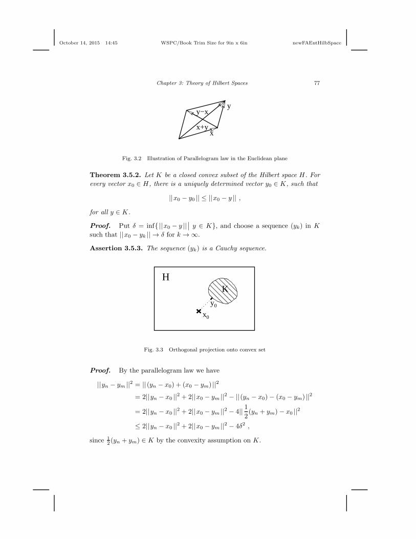
October 14, 2015 14:45 WSPC/Book Trim Size for 9in x 6in newFAEntHilbSpace
Chapter 3: Theory of Hilbert Spaces 77
x
y
x+y
y−x
Fig. 3.2 Illustration of Parallelogram law in the Euclidean plane
Theorem 3.5.2. Let K be a closed convex subset of the Hilbert space H. For
every vector x0 ∈ H, there is a uniquely determined vector y0 ∈ K, such that
||x0 − y0 || ≤ ||x0 − y || ,
for all y ∈ K.
Proof. Put δ = inf{||x0 − y ||∣∣ y ∈ K}, and choose a sequence (yk) in K
such that ||x0 − yk || → δ for k → ∞.
Assertion 3.5.3. The sequence (yk) is a Cauchy sequence.
����������������
����������������
y0
KH
0x
Fig. 3.3 Orthogonal projection onto convex set
Proof. By the parallelogram law we have
||yn − ym ||2 = ||(yn − x0) + (x0 − ym) ||2
= 2||yn − x0 ||2 + 2||x0 − ym ||2 − ||(yn − x0)− (x0 − ym) ||2
= 2||yn − x0 ||2 + 2||x0 − ym ||2 − 4|| 12(yn + ym)− x0 ||2
≤ 2||yn − x0 ||2 + 2||x0 − ym ||2 − 4δ2 ,
since 12 (yn + ym) ∈ K by the convexity assumption on K.
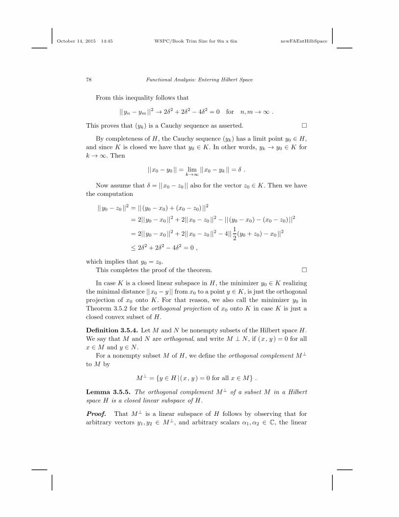
October 14, 2015 14:45 WSPC/Book Trim Size for 9in x 6in newFAEntHilbSpace
78 Functional Analysis: Entering Hilbert Space
From this inequality follows that
||yn − ym ||2 → 2δ2 + 2δ2 − 4δ2 = 0 for n,m→ ∞ .
This proves that (yk) is a Cauchy sequence as asserted. �
By completeness of H , the Cauchy sequence (yk) has a limit point y0 ∈ H ,
and since K is closed we have that y0 ∈ K. In other words, yk → y0 ∈ K for
k → ∞. Then
||x0 − y0 || = limk→∞
||x0 − yk || = δ .
Now assume that δ = ||x0 − z0 || also for the vector z0 ∈ K. Then we have
the computation
||y0 − z0 ||2 = ||(y0 − x0) + (x0 − z0) ||2
= 2||y0 − x0 ||2 + 2||x0 − z0 ||2 − ||(y0 − x0)− (x0 − z0) ||2
= 2||y0 − x0 ||2 + 2||x0 − z0 ||2 − 4|| 12(y0 + z0)− x0 ||2
≤ 2δ2 + 2δ2 − 4δ2 = 0 ,
which implies that y0 = z0.
This completes the proof of the theorem. �
In case K is a closed linear subspace in H , the minimizer y0 ∈ K realizing
the minimal distance ||x0 − y || from x0 to a point y ∈ K, is just the orthogonal
projection of x0 onto K. For that reason, we also call the minimizer y0 in
Theorem 3.5.2 for the orthogonal projection of x0 onto K in case K is just a
closed convex subset of H .
Definition 3.5.4. LetM and N be nonempty subsets of the Hilbert space H .
We say that M and N are orthogonal, and write M ⊥ N , if (x, y ) = 0 for all
x ∈M and y ∈ N .
For a nonempty subset M of H , we define the orthogonal complement M⊥
to M by
M⊥ = {y ∈ H |(x, y ) = 0 for all x ∈M} .
Lemma 3.5.5. The orthogonal complement M⊥ of a subset M in a Hilbert
space H is a closed linear subspace of H.
Proof. That M⊥ is a linear subspace of H follows by observing that for
arbitrary vectors y1, y2 ∈ M⊥, and arbitrary scalars α1, α2 ∈ C, the linear

October 14, 2015 14:45 WSPC/Book Trim Size for 9in x 6in newFAEntHilbSpace
Chapter 3: Theory of Hilbert Spaces 79
combination α1y1 + α2y2 belongs to M⊥, since
(x, α1y1 + α2y2 ) = α1 (x, y1 ) + α2 (x, y2 ) = 0 ,
for all x ∈M .
That M⊥ is a closed set follows by observing that if yn → y for n → ∞and yn ∈M⊥ for all n ∈ N, then y ∈M⊥, since
(x, y ) = limn→∞
(x, yn ) = 0 ,
for all x ∈M . �
Example 3.5.6. Let (en) be an orthonormal basis for the separable Hilbert
space H , and let I ⊆ N be an arbitrary subset of indexes. Then
M = span{ek |k ∈ I}
is a closed linear subspace of H . It is easy to prove that
M⊥ = {y ∈ H |(ek , y ) = 0 for all k ∈ I} .
Definition 3.5.7. Let M and N be closed linear subspaces of the Hilbert
space H , with M ⊥ N . Then we define the orthogonal sum M ⊕N of M and
N by
M ⊕N = {z ∈ H |z = x+ y, x ∈M, y ∈ N} .
Lemma 3.5.8. For the orthogonal sum M⊕N of two closed, orthogonal linear
subspaces M and N of the Hilbert space H it holds that
(a) The representation z = x+ y in M ⊕N is unique.
(b) M ⊕N is a closed linear subspace of H.
Proof. To prove (a), suppose that z = x1 + y1 = x2 + y2, where x1, x2 ∈M ,
y1, y2 ∈ N . Then x1 − x2 = y2 − y1 is a vector that belongs to both M and N .
Since M ⊥ N , it now follows that (x1 − x2 , x1 − x2 ) = (y1 − y2 , y1 − y2 ) = 0
and therefore that x1 = x2 and y1 = y2.
Next we prove (b). Clearly M ⊕ N is a linear subspace of H . To prove
that M ⊕N is a closed subspace, let (zn) be a convergent sequence of vectors
zn = xn + yn ∈ M ⊕ N with limit point z0 ∈ H . We have to prove that
z0 ∈M ⊕N . By Pythagoras’ theorem
||zn − zm ||2 = ||(xn − xm) + (yn − ym) ||2 = ||xn − xm ||2 + ||yn − ym ||2 .
From this follows easily that the sequences (xn) in M and (yn) in N are both
Cauchy sequences. Hence they are convergent in the Hilbert space H , say

October 14, 2015 14:45 WSPC/Book Trim Size for 9in x 6in newFAEntHilbSpace
80 Functional Analysis: Entering Hilbert Space
xn → x0 for n→ ∞ and yn → y0 for n→ ∞. Since both M and N are closed
subspaces in H it follows that x0 ∈M and y0 ∈ N . Furthermore,
z0 = limn→∞
zn = limn→∞
(xn + yn) = limn→∞
xn + limn→∞
yn = x0 + y0 .
This completes the proof of the lemma. �
In finite dimensions we have the well-known splitting Rn = Rn−k ⊕Rk, for
0 < k < n, obtained by identifying Rn−k with the subspace of Rn, where the
last k coordinates are zero, and Rk with the subspace of Rn, where the first
n−k coordinates are zero. In the Hilbert space setting we have a similar result,
known as the projection theorem.
Theorem 3.5.9 (The Projection Theorem). If M is a closed linear subspace
of the Hilbert space H, then H =M ⊕M⊥.
Proof. Let z ∈ H . According to the general orthogonal projection result for
closed convex subsets of H , Theorem 3.5.2, there exists a unique x ∈M , such
that ||z − x || ≤ ||z − x || for all x ∈ M . Put y = z − x. We now only have to
prove that y ∈M⊥.
If M = {0} this is obvious. If M 6= {0}, we consider the following compu-
tation valid for all λ ∈ C and x′ ∈M ,
||y ||2 = ||z − x ||2
≤ ||z − x− λx′ ||2
= ||y − λx′ ||2 = (y − λx′ , y − λx′ )
= ||y ||2 − λ(y , x′ )− λ(x′ , y ) + |λ |2||x′ ||2 .
By taking λ = (y , x′ ) and choosing x′ with ||x′ || = 1, we get
||y ||2 ≤ ||y ||2 − |λ |2 − |λ |2 + |λ |2 = ||y ||2 − |λ |2 .
This shows that necessarily (y , x′ ) = λ = 0 for all x′ ∈M with ||x′ || = 1, and
hence that (y , x′ ) = 0 for all x′ ∈M . In other words, y ∈M⊥, and the proof
is complete. �
We can now prove one of the most remarkable results in Hilbert space
theory, namely that for an arbitrary Hilbert space H , the dual space H∗ of
continuous linear functionals on H can be identified with H via the inner
product ( · , ·) in H . The theorem is due to the Hungarian mathematician
Frigyes Riesz (1880–1956), one of the pioneers in functional analysis.
October 14, 2015 14:45 WSPC/Book Trim Size for 9in x 6in newFAEntHilbSpace
Chapter 3: Theory of Hilbert Spaces 81
Theorem 3.5.10 (Riesz’ Representation Theorem). Let φ : H → C be a
continuous linear functional on a Hilbert space H. Then there is a unique
vector z ∈ H such that φ(x) = (x, z ) for all x ∈ H.
Proof. Let N = kerφ = {x ∈ H |φ(x) = 0} be the kernel of φ. Then N is a
linear subspace of H , and since φ is continuous, N is closed in H .
If N = H , the vector z = 0, and only this vector, will do.
If N 6= H , we can write H = N⊕N⊥ acoording to Theorem 3.5.9. Choose a
vector y0 ∈ N⊥ with ||y0 || = 1. Then surely φ(y0) 6= 0. For any vector x ∈ H ,
we can then write
φ(x) =φ(x)
φ(y0)φ(y0) = φ
( φ(x)φ(y0)
y0
).
This implies that
φ(x− φ(x)
φ(y0)y0
)= 0 ,
which shows that
x− φ(x)
φ(y0)y0 ∈ N .
Hence
0 = (x− φ(x)
φ(y0)y0 , y0 ) = (x, y0 )−
φ(x)
φ(y0).
It follows that
φ(x) = φ(y0)(x, y0 ) = (x, φ(y0) y0 ) .
Put z = φ(y0) y0. Then we have φ(x) = (x, z ) for all x ∈ H .
To prove uniqueness, assume that we have two representations φ(x) =
(x, v ) = (x, w ) for all x ∈ H . For x = v − w we then have the computation
0 = (x, v )− (x, w ) = (x, v − w ) = (v − w, v − w ) ,
which implies that v − w = 0, and hence v = w.
This completes the proof of Riesz’ Representation Theorem. �
3.6 Weak convergence
Definition 3.6.1. A sequence (xn) in a Hilbert space H is said to be weakly
convergent with weak limit x, if for all y ∈ H , the sequence of complex numbers

October 14, 2015 14:45 WSPC/Book Trim Size for 9in x 6in newFAEntHilbSpace
82 Functional Analysis: Entering Hilbert Space
((xn , y )
)has the limit (x, y ), in other words, if (xn , y ) → (x, y ) for n→ ∞,
for all y ∈ H .
If a sequence (xn) in H converges weakly to x ∈ H , we write xn ⇀ x for
n → ∞. In this context, ordinary convergence xn → x for n → ∞ is often
called strong convergence.
Remark 3.6.2. Using Riesz’ Representation Theorem, xn ⇀ x for n → ∞ if
and only if φ(xn) → φ(x) for n→ ∞ for every bounded linear functional φ on
H . In this formulation, the notion of weak convergence can also be introduced
in the more general setting of Banach spaces.
Lemma 3.6.3. If xn ⇀ x for n→ ∞, then the weak limit x ∈ H is unique.
Proof. Suppose xn ⇀ x and xn ⇀ z for n → ∞. Then (xn , y ) → (x, y )
and (xn , y ) → (z , y ) for n → ∞, for all y ∈ H . Since limits are unique in C,
it follows that (x, y ) = (z , y ) for all y ∈ H , and hence x− z ∈ H⊥ = {0}. �
Example 3.6.4. Let (en) be an orthonormal sequence in the Hilbert space
H . For y ∈ H , we have by Bessel’s inequality, Theorem 3.4.5, that the series∑∞n=1 |(y , en ) |2 is convergent and hence (en , y ) → 0 = (0 , y ) for n → ∞,
for all y ∈ H . This shows that en ⇀ 0 for n→ ∞.
On the other hand,
||en − em ||2 = ||en ||2 + ||em ||2 = 2 ,
for all n 6= m, so that (en) is not a Cauchy sequence, in particular, it is not
strongly convergent. This justifies the name weak convergence.
Proposition 3.6.5. Let (xn) be a sequence in the Hilbert space H. If (xn)
converges strongly to x for n→ ∞, then (xn) converges weakly to x for n→ ∞,
in other words, if xn → x for n→ ∞, then xn ⇀ x for n→ ∞.
Proof. If xn → x for n→ ∞, we have ||xn − x || → 0 for n→ ∞. From the
Cauchy-Schwarz inequality follows
|(xn , y )− (x, y ) | = |(xn − x, y ) | ≤ ||xn − x || ||y || for all y ∈ H .
This implies that (xn , y ) → (x, y ) for n → ∞, for all y ∈ H , proving that
xn ⇀ x for n→ ∞. �
The difference between strong convergence and weak convergence is a gen-
uine infinite dimensional phenomenon; if the Hilbert space is finite dimensional,
weak convergence will imply strong convergence.

October 14, 2015 14:45 WSPC/Book Trim Size for 9in x 6in newFAEntHilbSpace
Chapter 3: Theory of Hilbert Spaces 83
Theorem 3.6.6. Let H be a finite dimensional Hilbert space. Then every
weakly convergent sequence (xn) in H is strongly convergent.
Proof. Let {e1, . . . , ek} be an orthonormal basis for H . Then any vector
z ∈ H admits a unique decomposition
z = (z , e1 )e1 + · · ·+ (z , ek )ek .
Weak convergence of the sequence (xn) to x ∈ H implies (xn , ei ) → (x, ei )
for n→ ∞, for all i = 1, . . . , k. Hence
||x − xn ||2 =
k∑
i=1
|(x, ei )− (xn , ei ) |2 → 0 for n→ ∞ .
This proves that xn → x for n→ ∞ and hence completes the proof. �
Theorem 3.6.7. Every weakly convergent sequence in a Hilbert space H is
bounded.
Proof. Let (xn) be a weakly convergent sequence in the Hilbert space H
with weak limit x ∈ H . We have to prove that the sequence (xn) is bounded,
in other words, that the set of elements {xn} is a bounded subset of H .
We shall argue by contradiction. Hence we assume that the sequence (xn)
is unbounded. Clearly, the sequence (xn − x) is then also unbounded.
Let K ∈ R be a real number K > 1, which we shall specify later. We can
then extract a subsequence (yn) from the unbounded sequence (xn − x) such
that ||yn || ≥ Kn for each n ∈ N.
Now define the sequence (zn) in H by a recursive procedure. For n = 1 put
z1 = y1, and then for n ≥ 2,
zn = zn−1 +
K−n+1 (zn−1 , yn )| (zn−1 , yn ) |
yn
||yn || if (zn−1 , yn ) 6= 0
K−n+1 yn
||yn || if (zn−1 , yn ) = 0
.
Clearly, ||zn − zn−1 || = K−n+1 for each n ≥ 2. By the sum formula for a
geometric series, it then follows that
||zm − zn || <K−n
1−K−1
for all m > n ≥ 2. This proves that (zn) is a Cauchy sequence in the Hilbert
space H . Consequently, (zn) is convergent, say with limit z ∈ H .
First we consider the inner products (zn , yn ) for n ≥ 2.

October 14, 2015 14:45 WSPC/Book Trim Size for 9in x 6in newFAEntHilbSpace
84 Functional Analysis: Entering Hilbert Space
If on the one hand (zn−1 , yn ) 6= 0, we have
∣∣(zn , yn )∣∣ =
∣∣(zn−1 +K−n+1 (zn−1 , yn )
|(zn−1 , yn ) |yn
||yn ||, yn )
∣∣
=∣∣(zn−1 , yn ) + (zn−1 , yn )K
−n+1 (yn , yn )
|(zn−1 , yn ) |||yn ||∣∣
≥ K−n+1 |(zn−1 , yn ) |||yn ||2|(zn−1 , yn ) |||yn ||
=||yn ||Kn−1
.
If on the other hand (zn−1 , yn ) = 0, trivially
|(zn , yn ) | =||yn ||Kn−1
for each n ≥ 2 .
Next we consider the inner products (z , yn ) for n ≥ 2.
|(z , yn ) | = |(zn + z − zn , yn ) | = |(zn , yn ) + (z − zn , yn ) |≥ |(zn , yn ) | − |(z − zn , yn ) |≥ |(zn , yn ) | − ||z − zn || ||yn ||
≥ ||yn ||Kn−1
− K−n
1−K−1||yn ||
=K(1−K−1)− 1
(1−K−1)
||yn ||Kn
≥ K(1−K−1)− 1 = 1 if we put K = 3.
Now recall that (yn) is a subsequence of (xn−x). Hence the above argument
proves that there is a subsequence of ((z , xn − x)) that does not converge to
0, contradicting that the sequence (xn) converges weakly to x.
This completes the proof of the theorem. �
October 14, 2015 14:45 WSPC/Book Trim Size for 9in x 6in newFAEntHilbSpace
Chapter 4
Operators on Hilbert Spaces
Applications of functional analysis often involve operations by continuous lin-
ear mappings on the elements in a normed vector space, in particular, a Hilbert
space. The terminology used in this connection for such an operation is mostly
that of a bounded linear operator rather than a continuous linear mapping.
For a normed vector space V , we denote by
B(V ) the space of bounded linear operators T : V → V ,
in other words, the space of continuous linear mappings T : V → V .
4.1 The adjoint of a bounded linear operator
We open right away with the definition of the adjoint operator of a bounded
linear operator on a Hilbert space and its operator norm properties.
Theorem 4.1.1. Let H be a Hilbert space and T ∈ B(H) a bounded linear
operator on H. Then there is a unique bounded linear operator T ∗ ∈ B(H) on
H, called the adjoint operator of T , satisfying
(Tx, y ) = (x, T ∗y ) for all x, y ∈ H.
For the operator norms of T and T ∗, it holds that
||T ∗ || = ||T || and ||T ∗T || = ||T ||2.
Furthermore, it holds that
(T ∗)∗ = T and (ST )∗ = T ∗S∗,
for all bounded linear operators S, T ∈ B(H).
85

October 14, 2015 14:45 WSPC/Book Trim Size for 9in x 6in newFAEntHilbSpace
86 Functional Analysis: Entering Hilbert Space
Proof. For every vector y ∈ H , we can define a bounded linear functional
φy : H → C by φy(x) = (Tx, y ) for x ∈ H .
The functional φy is indeed linear, since T is linear and the inner product is
linear in the first argument. That φy is bounded follows by the computation,
using Cauchy-Schwarz’ inequality,
|φy(x) | = |(Tx, y ) | ≤ ||Tx || ||y || ≤ (||T || ||x ||) ||y || = (||T || ||y ||) ||x || .
By Riesz’ Representation Theorem, there is a unique z ∈ H such that
φy(x) = (x, z ) for all x ∈ H .
To every y ∈ H , there is in other words a uniquely determined z ∈ H for which
(Tx, y ) = (x, z ) for all x ∈ H .
We can therefore define a map T ∗ : H → H by letting T ∗(y) = z. The map
T ∗ is characterized by the equation
(Tx, y ) = (x, T ∗y ) for all x, y ∈ H .
Assertion 4.1.2. T ∗ is a linear operator.
Proof. For arbitrary vectors y1, y2 ∈ H and scalars α1, α2 ∈ C, we have the
following computation for every x ∈ H ,
(x, T ∗(α1y1 + α2y2)) = (Tx, α1y1 + α2y2 )
= α1 (Tx, y1 ) + α2 (Tx, y2 )
= α1 (x, T∗y1 ) + α2 (x, T
∗y2 )
= (x, α1T∗y1 + α2T
∗y2 ) .
Since this holds for all x ∈ H , we conclude that
T ∗(α1y1 + α2y2) = α1T∗y1 + α2T
∗y2 ,
completing the proof that T ∗ is linear. �
Assertion 4.1.3. T ∗ is bounded.
Proof. For y ∈ H , we have the computation
||T ∗y ||2 = (T ∗y , T ∗y ) = (T (T ∗y) , y )
≤ ||T (T ∗y) || ||y || ≤ ||T || ||T ∗y || ||y || .
October 14, 2015 14:45 WSPC/Book Trim Size for 9in x 6in newFAEntHilbSpace
Chapter 4: Operators on Hilbert Spaces 87
From this follows that
||T ∗y || ≤ ||T || ||y || for all y ∈ H .
[Trivial, if ||T ∗y || = 0; by division, if ||T ∗y || 6= 0.]
This proves that T ∗ is bounded, and furthermore, that ||T ∗ || ≤ ||T ||. �
Assertion 4.1.4. ||T ∗ || = ||T || and ||T ∗T || = ||T ||2.
Proof. Interchanging the roles of T and T ∗ in the argument showing that
||T ∗ || ≤ ||T ||, we get
||Tx ||2 = (Tx, Tx) = (x, T ∗(Tx))
≤ ||x || ||T ∗(Tx) || ≤ ||x || ||T ∗ || ||Tx || ,
from which follows,
||Tx || ≤ ||T ∗ || ||x || for all x ∈ H ,
proving that ||T || ≤ ||T ∗ ||. Altogether, we conclude that ||T || = ||T ∗ ||.For ||x || = 1, we have the computation
||Tx ||2 = (Tx, Tx) = (x, T ∗Tx) ≤ ||x || ||T ∗T || ||x || = ||T ∗T || ,
proving that ||T ||2 ≤ ||T ∗T ||.Since
||T ∗T || ≤ ||T ∗ || ||T || = ||T || ||T || = ||T ||2 ,
we get altogether ||T ∗T || = ||T ||2, completing the proof of the assertion. �
Assertion 4.1.5. (T ∗)∗ = T and (ST )∗ = T ∗S∗ for any pair of bounded linear
operators S, T ∈ B(H).
Proof. For all pairs of vectors x, y ∈ H , we have the computation
(Tx, y ) = (x, T ∗y ) = (T ∗y , x) = (y , (T ∗)∗x) = ((T ∗)∗x, y ) ,
from which follows that Tx = (T ∗)∗x for all x ∈ H , proving that (T ∗)∗ = T .
The computation
(x, (ST )∗y ) = (STx, y ) = (Tx, S∗y ) = (x, T ∗S∗y ) ,
valid for all x, y ∈ H , proves that
(ST )∗y = T ∗S∗y for all y ∈ H ,
or, in other words, that (ST )∗ = T ∗S∗. �
October 14, 2015 14:45 WSPC/Book Trim Size for 9in x 6in newFAEntHilbSpace
88 Functional Analysis: Entering Hilbert Space
This completes the proof of Theorem 4.1.1. �
Using Theorem 3.5.9 we can prove the following theorem.
Theorem 4.1.6. Every bounded linear operator T ∈ B(H) on a Hilbert space
H induces the orthogonal splitting
H = ker(T ∗)⊕ T (H) ,
where ker(T ∗) denotes the kernel of T ∗ and T (H) is the closure of the image
T (H) for T .
Proof. By the Projection Theorem,
H = T (H)⊥ ⊕ T (H) ,
valid for every closed linear subspace in H , in particular T (H) .
Assertion 4.1.7. T (H)⊥ = T (H)⊥ = ker(T ∗).
Proof. Let y ∈ T (H)⊥. Then
(x, T ∗y ) = (Tx, y ) = 0 for all x ∈ H ,
proving that T ∗y = 0, i.e. y ∈ ker(T ∗).
On the other hand, let y ∈ ker(T ∗). Then
(Tx, y ) = (x, T ∗y ) = (x, 0) = 0 for all x ∈ H ,
proving that y ∈ T (H)⊥.
Altogether, T (H)⊥ = ker(T ∗). It is easy to prove that T (H)⊥ = T (H)⊥.
This completes the proof of the assertion and hence of the theorem. �
Example 4.1.8. A bounded linear operator T : Ck → Ck is represented by
a k × k-matrix [Tij ] with respect to the canonical basis {e1, . . . , ek} in Ck.
In terms of the inner product in Ck, the matrix elements are determined by
Tij = (Tej , ei ).
Let [T ∗ij ] be the matrix representing the adjoint operator T ∗ : Ck → Ck.
Then
T ∗ij = (T ∗ej , ei ) = (ei , T ∗ej ) = (Tei , ej ) = Tji .
Conclusion: The matrix representation for the adjoint linear operator T ∗ is the
conjugate transpose of the matrix representation for T .

October 14, 2015 14:45 WSPC/Book Trim Size for 9in x 6in newFAEntHilbSpace
Chapter 4: Operators on Hilbert Spaces 89
In the case of real vector spaces, the adjoint operator T ∗ : Rk → Rk for a
bounded linear operator T : Rk → Rk is represented by the transposed matrix
to the matrix representing T .
Definition 4.1.9. Let H be a Hilbert space. A bounded linear operator T on
H is called self-adjoint if T = T ∗.
Lemma 4.1.10. Let T be a bounded, self-adjoint linear operator on a Hilbert
space H. Then (Tx, x) is a real number for all x ∈ H.
Proof. For every x ∈ H , we have the computation
(Tx, x) = (x, T ∗x) = (x, Tx) = (Tx, x) ,
proving that (Tx, x) is a real number. �
For self-adjoint operators, there is an alternative method to determine the
operator norm.
Theorem 4.1.11. Let T be a bounded, self-adjoint linear operator on a Hilbert
space H. Then
||T || = sup{|(Tx, x) |∣∣ x ∈ H, ||x || = 1} .
Proof. For each vector x ∈ H with ||x || = 1, we get by the Cauchy-Schwarz
inequality,
|(Tx, x) | ≤ ||Tx || ||x || ≤ ||T || ||x ||2 = ||T || .
This proves that the number
MT = sup{|(Tx, x) |∣∣ x ∈ H, ||x || = 1}
exists, and that MT ≤ ||T ||.A simple calculation shows that
(T (x+ y) , x+ y )− (T (x− y) , x− y ) = 2(Tx, y ) + 2(Ty , x) ,
where each term on the left-hand side is a real number since T is self-adjoint.
From the definition of MT follows that
(T (x+ y) , x+ y ) ≤ MT ||x+ y ||2 ,−(T (x− y) , x− y ) ≤ MT ||x− y ||2 .
To prove these inequalities, write x+ y = ||x+ y ||u and x− y = ||x− y ||vfor unit vectors u, v ∈ H .

October 14, 2015 14:45 WSPC/Book Trim Size for 9in x 6in newFAEntHilbSpace
90 Functional Analysis: Entering Hilbert Space
Using the parallelogram law, Proposition 3.5.1, for the second inequality
we get,
(Tx, y ) + (Ty , x) =1
2
((T (x+ y) , x+ y )− (T (x− y) , x− y )
)
≤ 1
2MT
(||x+ y ||2 + ||x− y ||2
)
≤ MT
(||x ||2 + ||y ||2
).
Assertion 4.1.12. ||Tx || ≤MT ||x || for all x ∈ H.
Proof. The assertion is trivial for Tx = 0. So assume that Tx 6= 0. Put
y =||x ||||Tx || Tx .
Then we have the computations,
(Tx, y ) + (Ty , x) =||x ||||Tx || (Tx, Tx) +
||x ||||Tx || (T (Tx) , x)
= ||x || ||Tx ||+ ||x ||||Tx || (Tx, T
∗x)
= ||x || ||Tx ||+ ||x ||||Tx || (Tx, Tx) (T ∗ = T )
= 2 ||x || ||Tx || .
MT
(||x ||2 + ||y ||2
)= MT
(||x ||2 + ||x ||2
||Tx ||2 ||Tx ||2)= 2MT ||x ||2 .
By the inequality preceding the assertion we conclude that
||Tx || ≤MT ||x || for all x ∈ H ,
as asserted. �
From the assertion we infer that ||T || ≤ MT . Together with the already
established inequality MT ≤ ||T || this proves that ||T || = MT , and the proof
of the theorem is complete. �
In finite dimensions we know that a linear operator T : Ck → Ck is injec-
tive if and only if it is surjective. For self-adjoint linear operators we have a
corresponding result in the Hilbert space case, valid also in infinite dimensions.

October 14, 2015 14:45 WSPC/Book Trim Size for 9in x 6in newFAEntHilbSpace
Chapter 4: Operators on Hilbert Spaces 91
Theorem 4.1.13. Let T be a bounded, self-adjoint linear operator on a Hilbert
space H. If T (H) is dense in H, then T has an inverse operator defined on the
image T (H) of T .
Proof. By Theorem 4.1.6 we get the splitting H = ker(T ∗) ⊕ T (H) from
which follows that ker(T ∗) = {0}, since T (H) is dense in H . But then ker(T ) =
{0}, since T ∗ = T , proving that T is injective. Altogether, we have a well-
defined inverse linear operator T−1 : T (H) → H as stated in the theorem. �
Remark 4.1.14. The inverse linear operator T−1 in Theorem 4.1.13 is not
necessarily bounded; in fact, most often in applications it is not! If T−1 is
unbounded, its domain of definition cannot be extended to all of H , since it is
equivalent for T−1 to be bounded and to admit an extension from the dense
subspace T (H) to all of H . That these statements are equivalent follows since
the inverse mapping for a bijective, bounded linear mapping between Banach
spaces is always bounded. The latter fact is a corollary to the famous Open
Mapping Theorem known as Banach’s Theorem 1.8.3.
Theorem 4.1.15. Let P be a bounded, self-adjoint linear operator on the
Hilbert space H, and assume that P is an idempotent operator, i.e. P 2 = P .
Then P is the orthogonal projection onto the closed linear subspace
M = {z ∈ H∣∣Pz = z} (fixed space for P ).
Proof. Let I : H → H denote the identity operator on H , i.e. I(z) = z for
all z ∈ H . Then
M = {z ∈ H∣∣Pz = z} = {z ∈ H
∣∣(P − I)z = 0} = ker(P − I) .
Since P−I is a continuous linear operator on H , it follows from the description
of M as the kernel of P − I that M is a closed linear subspace in H .
By Theorem 3.5.9, we then have the orthogonal splitting
H =M ⊕M⊥ .
Hence every vector z ∈ H admits a unique decomposition,
z = x+ y, x ∈M, y ∈M⊥ .
From the decomposition z = x + y with x ∈ M and y ∈ M⊥, we get
Pz = Px + Py = x + Py. Since P (Py) = P 2y = Py, we have Py ∈ M .
But Py also belongs to M⊥. This follows from the computation (x, Py ) =
(Px, y ) = (x, y ) = 0, valid for all x ∈M . Since M ∩M⊥ = {0}, we conclude
that Py = 0.

October 14, 2015 14:45 WSPC/Book Trim Size for 9in x 6in newFAEntHilbSpace
92 Functional Analysis: Entering Hilbert Space
For z = x+ y, x ∈M, y ∈M⊥, it follows altogether that Pz = x. In other
words, P is exactly the orthogonal projection onto the fixed space M for P ,
and the proof is complete. �
For obvious reasons, a bounded, self-adjoint, idempotent linear operator
P on a Hilbert space H is called a projection operator. As we have seen in
Theorem 4.1.15, a projection operator is exactly the orthogonal projection
onto the corresponding fixed space.
Proposition 4.1.16. For a projection operator P on a Hilbert space H, the
operator norm satisfies ||P || ≤ 1. If P 6= 0, the operator norm ||P || = 1.
Proof. For all x ∈ H we have the computation
||Px ||2 = (Px, Px) = (P 2x, x) = (Px, x) ≤ ||Px || ||x || ,
proving that ||Px || ≤ 1 for all x ∈ H with ||x || = 1. It follows that ||P || ≤ 1.
If P 6= 0, the fixed space M = {z ∈ H∣∣Pz = z} for P contains nonzero
vectors [with z = Pu, we have Pz = P (Pu) = P 2u = Pu = z]. For a unit
vector x ∈ M , we have ||Px || = ||x || = 1, and consequently, the operator
norm must be ||P || = 1. �
4.2 Compact operators
In a metric space, in particular in a normed vector space, the notions of com-
pactness (defined by the covering property) and sequential compactness (every
sequence contains a convergent subsequence) are equivalent notions. When the
notion of compactness is used in normed vector spaces, we are therefore free
to use the definition most suitable for our purposes. In functional analysis it
is often convenient to use the definition: A subset K in a normed vector space
V is compact, if every sequence (xn) of elements in K contains a convergent
subsequence (xnk) with limit point x ∈ K.
In a finite dimensional normed vector space V we know by the Heine-Borel
Theorem that a subset K ⊆ V is compact if and only if it is a closed and
bounded subset.
It is always true that a compact subset K ⊆ V of a normed vector space V
is closed and bounded. In general, the converse is only true in finite dimensions.
Example 4.2.1. Let H be a separable Hilbert space. Consider the unit ball
C = {x ∈ H∣∣ ||x || ≤ 1} .
October 14, 2015 14:45 WSPC/Book Trim Size for 9in x 6in newFAEntHilbSpace
Chapter 4: Operators on Hilbert Spaces 93
Clearly, C is a closed and bounded subset of H . But C is not compact if H is
infinite dimensional. This follows since an arbitrary orthonormal sequence (xn)
in H is contained in C and has no convergent subsequence (xnk); a subsequence
is not even a Cauchy sequence, since ||xni− xnj
||2 = 2 for all i 6= j.
The result in Example 4.2.1 holds in complete generality in a normed vector
space. To prove this we need a famous result known as Riesz’ Lemma.
Lemma 4.2.2 (Riesz’ Lemma). Let V be a normed vector space and let U
be a closed subspace of V with U 6= V . Let α be a real number in the interval
0 < α < 1. Then there exists a vector v ∈ V such that
||v || = 1 and ||v − u || ≥ α for all u ∈ U .
Proof. Choose an arbitrary vector v0 ∈ V \U . Since U is a closed subspace
of V , the distance of v0 to U is strictly positive, i.e.
inf{||v0 − u || |u ∈ U} = r0 > 0 .
Since r0 < r0/α, when 0 < α < 1, we can choose u0 ∈ U such that
||v0 − u0 || ≤r0α.
Put v = (v0 − u0)/||v0 − u0 ||. Then ||v || = 1 and
||v − u || = ||v0 − u0 − ||v0 − u0 || u ||||v0 − u0 ||
≥ r0||v0 − u0 ||
≥ α ,
for all u ∈ U . This completes the proof. �
Theorem 4.2.3. Let V be an arbitrary normed vector space, and let
C = {x ∈ V∣∣ ||x || ≤ 1}
be the closed unit ball in V .
Then C is compact if and only if V has finite dimension.
Proof. First assume that C is compact and that V is not finite dimen-
sional. Choose an arbitrary element x1 ∈ V with ||x1 || = 1. Let U1 be the 1-
dimensional, and hence closed, subspace of V spanned by x1. By Riesz’ Lemma
4.2.2, there exists x2 ∈ V \U1 with ||x2 || = 1 and ||x2 − x1 || ≥ 1/2. Let U2 be
the 2-dimensional, and hence closed, subspace of V spanned by {x1, x2}. Againby Riesz’ Lemma, there exists x3 ∈ V \U2 with ||x3 || = 1 and ||x3 − x1 || ≥ 1/2,
||x3 − x2 || ≥ 1/2. Continuing by induction, we find a sequence (xn) of linearly
independent vectors in V with the properties ||xn || = 1 and ||xn − xm || ≥ 1/2,
October 14, 2015 14:45 WSPC/Book Trim Size for 9in x 6in newFAEntHilbSpace
94 Functional Analysis: Entering Hilbert Space
for n 6= m. By construction, the sequence (xn) in C does not contain a conver-
gent subsequence. This contradicts that C is compact. Therefore necessarily V
has finite dimension if C is compact.
Conversely, if V is finite dimensional, then C is compact by the Heine-Borel
Theorem 1.3.12, since it is a closed and bounded subset in V . �
A linear operator between normed vector spaces is by definition a bounded,
or, continuous, operator if it maps bounded subsets in the domain vector space
into bounded subsets in the image vector space. A compact, or, completely
continuous, operator has a stronger property.
Definition 4.2.4. Let V and W be normed vector spaces. A bounded linear
operator T : V →W is said to be a compact, or completely continuous, operator
if it maps every bounded subset A in V into a subset T (A) in W with compact
closure T (A) in W .
By Example 4.2.1, the unit ball in a Hilbert space H is not compact in infi-
nite dimension. Hence the identity operator I on H is not compact. Somehow,
compactness of an operator is related to finite dimensionality of its image.
Definition 4.2.5. A bounded linear operator T : V → W between normed
vector spaces V and W is said to have finite rank if dimT (V ) is finite, where
dimT (V ) is the dimension of the linear subspace in W formed by the image
for T in W .
Proposition 4.2.6. A bounded linear operator of finite rank is a compact
operator.
Proof. Let T : V →W be a bounded linear operator between normed vector
spaces V and W for which dimT (V ) is finite. Since T is bounded, it maps a
bounded subset A ⊆ V into a bounded subset T (A) ⊆ T (V ) ⊆ W . Also the
closure T (A) is contained in T (V ), since T (V ) is finite dimensional and hence
a closed linear subspace in W . Consequently, T (A) is bounded and closed in
a finite dimensional vector space and therefore compact. �
In finite dimensions, weak convergence coincides with convergence in norm
and hence it is to be expected that compact linear operators behave well with
respect to weak convergence. This is indeed true, and the following result
motivates why compact linear operators are also called completely continuous
operators.
Theorem 4.2.7. Let H be a Hilbert space and let (xn) be a weakly convergent
sequence with weak limit x. Then for every compact linear operator T on H,
October 14, 2015 14:45 WSPC/Book Trim Size for 9in x 6in newFAEntHilbSpace
Chapter 4: Operators on Hilbert Spaces 95
the image sequence (Txn) converges strongly (in norm) to Tx. In other words:
For a compact linear operator T ∈ B(H) it holds that
xn ⇀ x for n→ ∞ ⇒ Txn → Tx for n→ ∞ .
Proof. If xn ⇀ x for n→ ∞ we have for all y ∈ H ,
(Txn , y ) = (xn , T∗y ) → (x, T ∗y ) = (Tx, y ) for n→ ∞ .
This proves that Txn ⇀ Tx for n → ∞. Since weak limits are unique and
strong convergence implies weak convergence, the only possible strong limit
for (Txn) is Tx.
Assertion 4.2.8. Txn → Tx for n→ ∞.
Proof. The proof is indirect. Suppose (Txn) does not converge in norm to
Tx. Then we can extract a subsequence (Txnk) of (Txn) such that
||Txnk− Tx || ≥ δ for all k ∈ N and some δ > 0 .
Since (xn) is bounded by Theorem 3.6.7 and T is a compact linear operator,
we can extract a subsequence (Txnkl) of (Txnk
) for which Txnkl→ y ∈ H for
l → ∞. Since Txnkl⇀ Tx for l → ∞, we must have y = Tx, which is not
possible by the construction of Txnk. Thereby we have obtained a contradiction
and hence Txn → Tx for n→ ∞. �
This completes the proof of the theorem. �
Example 4.2.9. Let (en) be an orthonormal sequence in the Hilbert space
H . From Example 3.6.4 we know that en ⇀ 0 for n→ ∞. Hence by Theorem
4.2.7 we conclude that Ten → 0 for n→ ∞ for every compact linear operator
T ∈ B(H).
From the example we infer that the inverse operator (if it exists) of a
compact linear operator on a separable Hilbert space is always unbounded.
Proposition 4.2.10. Let H be an infinite dimensional, separable Hilbert
space. Suppose T ∈ B(H) is a compact linear operator on H, which has an
inverse T−1 on T (H). Then T−1 is always an unbounded linear operator.
Proof. Let (en) be an orthonormal sequence in H ; for example an or-
thonormal basis in H . Then Ten → 0 for n → ∞, but on the other hand,
||T−1(Ten) || = ||en || = 1 for all n ∈ N, and hence T−1 cannot be continuous.
In other words, the linear operator T−1 is unbounded. �
October 14, 2015 14:45 WSPC/Book Trim Size for 9in x 6in newFAEntHilbSpace
96 Functional Analysis: Entering Hilbert Space
The set of compact linear operators on a Hilbert space H is a closed subset
in the Banach space (operator norm) of bounded linear operators B(H) on H .
This is a consequence of the following theorem.
Theorem 4.2.11. Let H be a Hilbert space and suppose that (Tn) is a sequence
of compact linear operators in B(H) converging (in operator norm) to the
bounded linear operator T ∈ B(H). Then T is a compact linear operator.
Proof. It is sufficient to prove that if (xn) is a bounded sequence in H , then
it is possible to extract a subsequence (xnk) such that (Txnk
) is convergent.
Let (xn) be a bounded sequence in H . Since T1 is compact, (xn) has a
subsequence (x1n) such that (T1x1n) is convergent. Since T2 is compact, (x1n) has
a subsequence (x2n) such that (T2x2n) is convergent. Continuing this way we get
for every k ∈ N, a subsequence (xkn) of (xn) such that (Tkxkn) is convergent. Now
consider the diagonal sequence (xnn). It is obvious that (Tkxnn) is convergent for
every k ∈ N.
Assertion 4.2.12. (Txnn) is a Cauchy sequence in H.
Proof. Given ε > 0.
Since the original sequence (xn) is bounded, there exists a positive constant
C such that ||xnn || ≤ C for all n ∈ N.
Since Tn → T for n → ∞ (in operator norm), we can choose a number
k ∈ N, which we then keep fixed, such that
||T − Tk || ≤ε
3C.
Since (Tkxnn) is convergent, there exists a number n0 ∈ N, such that
||Tkxnn − Tkxmm || ≤ ε
3for all n,m ≥ n0 .
For n,m ≥ n0 we now have the computation
||Txnn − Txmm || ≤ ||Txnn − Tkxnn ||+ ||Tkxnn − Tkx
mm ||+ ||Tkxmm − Txmm ||
≤ ||T − Tk || ||xnn ||+ε
3+ ||Tk − T || ||xmm ||
≤ ε
3CC +
ε
3+
ε
3CC = ε .
This proves that (Txnn) is indeed a Cauchy sequence in H . �
By completeness of H , the Cauchy sequence (Txnn) is convergent in H .
Since (xnn) is a subsequence of (xn), this proves that T is a compact linear
operator. �
October 14, 2015 14:45 WSPC/Book Trim Size for 9in x 6in newFAEntHilbSpace
Chapter 4: Operators on Hilbert Spaces 97
The following theorem provides among others a method for constructing
compact linear operators.
Theorem 4.2.13. Let (en) be an orthonormal basis for the infinite dimen-
sional, separable Hilbert space H and let (λn) be an arbitrary sequence of com-
plex numbers. For every x ∈ H, consider the infinite series
Tx =
∞∑
n=1
λn(x, en )en .
(1) The infinite series is convergent and the sum defines a linear operator
T on H if the sequence (λn) is bounded.
(2) T exists and is bounded if and only if the sequence (λn) is bounded.
(3) T exists and is a compact linear operator if and only if λn → 0 for
n→ ∞.
Proof. The series∑∞
n=1(x, en )en is convergent for all x ∈ H by Theorem
3.4.5 (Bessel’s inequality). Then by the comparison test, the infinite series
Tx =∑∞
n=1 λn(x, en )en is also convergent for all x ∈ H if the sequence (λn)
is bounded, in particular, if λn → 0 for n→ ∞. In case of existence, clearly T
is a linear operator. This proves (1).
Since
||Tx ||2 =
∞∑
n=1
|λn |2|(x, en ) |2 and ||x ||2 =
∞∑
n=1
|(x, en ) |2 ,
and since ||Ten || = |λn | for all n ∈ N, it follows immediately that T exists
and is bounded if and only if the sequence (λn) is bounded. This proves (2).
In order to prove (3), we define the sequence of operators (Tk) by
Tkx =k∑
n=1
λn(x, en )en for all x ∈ H .
Since Tk has finite rank, all the operators Tk are compact linear operators by
Proposition 4.2.6.
When the sequence (λn) is bounded, we can define the bounds
Kk = supn>k
{|λn |2} for all k ∈ N .
Then for all k ∈ N, we get the estimate
||Tx− Tkx ||2 =
∞∑
n=k+1
|λn |2|(x, en ) |2 ≤ Kk||x ||2 .

October 14, 2015 14:45 WSPC/Book Trim Size for 9in x 6in newFAEntHilbSpace
98 Functional Analysis: Entering Hilbert Space
From this estimate follows that ||T − Tk || ≤√Kk and hence that
||T − Tk || → 0 for k → ∞, if λn → 0 for n→ ∞ .
This proves that Tk → T for k → ∞, and hence by Theorem 4.2.11 that T is
a compact linear operator, if λn → 0 for n→ ∞.
Now assume that the sequence (λn) does not converge to 0 for n → ∞.
Then there exist an ε > 0 and a subsequence (λnk) of (λn) such that |λnk
| ≥ ε
for all k ∈ N. Consider the corresponding subsequence (enk) of (en). Being an
orthonormal sequence, (enk) is weakly convergent to 0. Since
||Teni− Tenj
||2 = ||λnieni
− λnjenj
||2 = |λni|2 + |λnj
|2 ≥ 2ε2 ,
for all i 6= j, the sequence (Tenk) can have no subsequences that are Cauchy
sequences, and hence in particular, (Tenk) does not converge to 0. From this
we conclude by Theorem 4.2.7 that T is not a compact linear operator.
This completes the proof of the theorem. �
Example 4.2.14. Let (en) be an orthonormal basis in the infinite dimensional,
separable Hilbert space H . Define
Tx =
∞∑
n=1
1
n(x, en )en for all x ∈ H .
Then T is a compact linear operator on H by Theorem 4.2.13. The following
computation shows that the operator T is self-adjoint,
(Tx, y ) =∞∑
n=1
1
n(x, en )(y , en ) = (x, T y ) for all x, y ∈ H .
Since T (kek) = ek for all k ∈ N, it follows that T (H) is dense inH . Hence T has
an inverse operator T−1 : T (H) → H by Theorem 4.1.13. Since T−1(ek) = kekfor all k ∈ N, clearly T−1 is unbounded.

October 14, 2015 14:45 WSPC/Book Trim Size for 9in x 6in newFAEntHilbSpace
Chapter 5
Spectral Theory
A linear map T : Ck → Ck is represented by a complex k × k-matrix with
respect to the canonical basis in Ck. If the linear map T is self-adjoint, we
know from Example 4.1.8 that it is represented by a conjugate symmetric
matrix. From basic linear algebra, it is then well known that there exists an
orthonormal basis {ej}kj=1 for Ck in which the matrix for T can be diagonalized,
or, which amounts to the same thing, that the linear map itself is given by
Tx =
k∑
j=1
λj(x, ej )ej , for all x ∈ Ck .
Here (x, ej ) is the jth coordinate of x in an orthonormal basis {ej}kj=1 of
eigenvectors for T corresponding to the eigenvalues {λj}kj=1 for T .
The eigenvalues for T are the complex numbers λ, for which the equation
Tx = λx has nontrivial solutions x ∈ Ck, or, by an equivalent formulation, for
which the linear operator T − λI is not injective, where I denotes the identity
operator on Ck.
In infinite dimensions, the situation is much more complicated, but for self-
adjoint, compact linear operators a corresponding theory can be developed. It
culminates in the famous spectral theorem - the main goal of this chapter.
5.1 The spectrum and the resolvent
Let H be a Hilbert space and let T : H → H be a linear operator. Often in
the following, a linear operator T may not be defined on all of H but only on
a linear subspace of H called the domain of definition and denoted by D(T ).
Let T : H → H be a linear operator with domain of definition D(T ) ⊆ H .
99

October 14, 2015 14:45 WSPC/Book Trim Size for 9in x 6in newFAEntHilbSpace
100 Functional Analysis: Entering Hilbert Space
For λ ∈ C, we define the linear operator
Tλ = T − λI with D(Tλ) = D(T ) ,
where I denotes the identity operator on H .
Remark 5.1.1. Integral equations of the form
(T − λI)u = f for u, f ∈ L2([a, b]), λ ∈ C ,
defined in the Hilbert space H = L2([a, b]), are known under the name of
Fredholm integral equations of the second kind. They occur frequently in ap-
plications in the physical sciences.
In the general setting presented above, we consider the equation
Tλx = y for each y ∈ H .
If Tλ is injective, we can solve the equation to get
x = T−1λ y for all y ∈ Tλ(H) = D(T−1
λ ) .
If T−1λ is also bounded, and Tλ(H) = D(T−1
λ ) is dense in H , then T−1λ admits
a unique extension to all of H , such that the equation Tλx = y can be solved
for all y ∈ H . This is the ideal situation from the point of view of the equation.
However, it will not always be the case.
The operator
Rλ(T ) = T−1λ = (T − λI)−1 ,
defined for those λ ∈ C where Tλ is injective, is called the resolvent of T . We
are particularly interested in the situation where D(Rλ(T )) = Tλ(H) is dense
in H and Rλ(T ) is a bounded linear operator.
Definition 5.1.2. The resolvent set for T , denoted by ρ(T ), is the set of λ ∈ C
for which Rλ(T ) exists as a densely defined and bounded linear operator on
H . The complement σ(T ) = C \ ρ(T ) is called the spectrum for T .
For λ ∈ σ(T ) various things can happen. First of all, maybe the linear map
Tλ is not injective so that the resolvent Rλ(T ) is not defined. This is the case
if and only if the equation
(T − λI)x = 0 has a nontrivial solution x ∈ H ,
or equivalently,
Tx = λx for a nontrivial vector x ∈ H .

October 14, 2015 14:45 WSPC/Book Trim Size for 9in x 6in newFAEntHilbSpace
Chapter 5: Spectral Theory 101
If this is the case, we say that λ is an eigenvalue of T , with corresponding
eigenvector x ∈ H . The equation Tx = λx is always satisfied for x = 0 and
hence we emphasize that in order for λ to be an eigenvalue for T , the equation
shall be satisfied for an eigenvector x 6= 0. Furthermore, we notice that the
collection of all eigenvectors, belonging to an eigenvalue λ, form a linear sub-
space Hλ of H , called the eigenspace corresponding to λ. The linear subspace
Hλ can be of finite or infinite dimension depending on the case in question.
Definition 5.1.3. The subset σP (T ) of the spectrum σ(T ) for T consisting of
the eigenvalues for T is called the point spectrum for T .
The subset σC(T ) of the spectrum σ(T ) for T consisting of the complex
numbers λ ∈ C for which Rλ(T ) exists as a densely defined but unbounded
operator on H , is called the continuous spectrum for T .
Finally, the subset σr(T ) of the spectrum σ(T ) for T , where Rλ(T ) exists
but is not densely defined, is called the residual spectrum for T .
All possibilities for λ ∈ σ(T ) are covered by Definition 5.1.3, and hence the
spectrum σ(T ) for T is the disjoint union of the point spectrum, the continuous
spectrum and the residual spectrum for T . In concrete cases, the resolvent set
ρ(T ) and/or parts of the spectrum for T may be empty.
Example 5.1.4. Let T : Ck → Ck be a linear map with corresponding matrix
T = [Tij ]. Then it is well known that T has k eigenvalues λ1, . . . , λk (counted
with multiplicity) and that the eigenvalues are the roots of the characteristic
polynomial P (λ) = det(T−λI) for T . Since Rλ(T ) ∈ B(Ck), when λ is not an
eigenvalue, it follows that the spectrum σ(T ) is a pure point spectrum, namely
σ(T ) = {λj}kj=1, and that the resolvent set is the complex plane except finitely
many points, namely ρ(T ) = C \ {λj}kj=1.
Example 5.1.5. Let ∂ = d/dx be the differentiation operator with domain of
definition D(∂) = C1([0, 1]) in the Hilbert space H = L2([0, 1]). Then
(∂ − λI)eλx = 0 for all λ ∈ C .
It follows that the spectrum σ(∂) is a pure point spectrum, namely σ(∂) = C,
and consequently, that the resolvent set ρ(∂) = C \ σ(∂) = ∅.
The unbounded linear operator ∂ in Example 5.1.5 has an empty resolvent
set. On the other hand, this is never the case for a bounded linear operator.
This will be an immediate consequence of interesting topological properties of
the spectrum for a bounded linear operator. For the proof of these properties,
we need a general result on existence of bounded inverse operators for small
October 14, 2015 14:45 WSPC/Book Trim Size for 9in x 6in newFAEntHilbSpace
102 Functional Analysis: Entering Hilbert Space
perturbations of an identity operator proved by the German mathematician
Carl Gottfried Neumann (1832–1925).
Lemma 5.1.6 (Neumann’s Lemma). Let V be an arbitrary Banach space, and
let T ∈ B(V ) be a bounded linear operator with operator norm ||T || < 1. Then
the operator I − T has a bounded inverse operator (I − T )−1 on V .
Proof. Consider the infinite series,
S = I +
∞∑
n=1
T n = I + T + T 2 + · · ·+ T n + . . . ,
in the Banach space B(V ). The series is convergent in B(V ) by the comparison
test, since
||T n || ≤ ||T ||n for all n ∈ N ,
and the geometric series∑∞
n=0 ||T ||n is convergent, since ||T || < 1.
Elementary computations show that
S(I − T ) = I = (I − T )S .
This proves that I − T is invertible with inverse operator (I − T )−1 = S. �
Then we are ready to study the topological properties of the resolvent set
ρ(T ) and the spectrum σ(T ) for a bounded linear operator T on a Hilbert
space H .
Theorem 5.1.7. Let H be a Hilbert space and let T ∈ B(H) be a bounded
linear operator on H. Then the resolvent set ρ(T ) for T is an open set in C
and the spectrum σ(T ) for T is a closed set in C.
Proof. If ρ(T ) = ∅, the theorem is trivially true.
Assume therefore that ρ(T ) 6= ∅. Let µ ∈ ρ(T ) be an arbitrary point in
ρ(T ). Then Rµ(T ) = (T −µI)−1 is a densely defined, bounded linear operator.
For λ ∈ C, we have
T − λI = (T − µI)− (λ − µ)I = (T − µI)(I − (λ− µ)Rµ(T )
).
By Neumann’s Lemma, this rewriting shows that T−λI is an invertible, densely
defined (namely on Tµ(H)) operator with bounded inverse, when
||(λ− µ)Rµ(T ) || = |λ− µ | ||Rµ(T ) || < 1 ,
in other words, for |λ− µ | < ||Rµ(T ) ||−1. This describes a circle in C with
center µ, thereby proving that ρ(T ) is an open set in C.
October 14, 2015 14:45 WSPC/Book Trim Size for 9in x 6in newFAEntHilbSpace
Chapter 5: Spectral Theory 103
Since σ(T ) = C \ ρ(T ), the spectrum σ(T ) is a closed set in C. �
Theorem 5.1.8. Let H be a Hilbert space and let T ∈ B(H) be a bounded
linear operator on H. Then the spectrum σ(T ) for T is a compact set in C,
contained in the circle with radius ||T || and center 0.
Proof. Assume that |λ | > ||T ||. Then
T − λI = −λ(I − 1
λT)
has a bounded inverse, since ||(1/λ)T || < 1, and hence λ ∈ ρ(T ). Consequently,
λ ∈ σ(T ) implies that |λ | ≤ ||T ||, proving that σ(T ) is a bounded set in C.
But σ(T ) is also a closed set in C, and hence σ(T ) is a compact set in C. �
Remark 5.1.9. For a bounded linear operator T ∈ B(H) it follows in particular
that λ ∈ ρ(T ) for |λ | > ||T ||. Hence ρ(T ) 6= ∅ for a bounded linear operator.
5.2 Spectral theorem for compact self-adjoint operators
We now turn our attention to bounded, self-adjoint linear operators T on a
Hilbert space H . For such an operator T , we have the alternative formula for
the operator norm ||T || proved in Theorem 4.1.11,
||T || = sup{|(Tx, x) |∣∣ x ∈ H, ||x || = 1} .
Hence we get the following corollary from Theorem 5.1.8.
Corollary 5.2.1. Let T be a bounded, self-adjoint linear operator on a Hilbert
space H. Then for all λ ∈ σ(T ) in the spectrum for T it holds that
|λ | ≤ sup{|(Tx, x) |∣∣ x ∈ H, ||x || = 1} .
Example 5.2.2. Let (en) be an orthonormal basis for the infinite dimensional,
separable Hilbert space H . Then the one-sided shift operator T on H with
respect to this basis is defined by
T (x) = T( ∞∑
n=1
(x, en )en
)=
∞∑
n=2
(x, en )en−1 for all x ∈ H .
We shall determine the spectrum σ(T ) for T . For that purpose, suppose
x =
∞∑
n=1
(x, en )en is an eigenvector for T ,

October 14, 2015 14:45 WSPC/Book Trim Size for 9in x 6in newFAEntHilbSpace
104 Functional Analysis: Entering Hilbert Space
with corresponding eigenvalue λ. Then we get recursively,
(x, e2 ) = λ(x, e1 )
(x, e3 ) = λ(x, e2 ) = λ2(x, e1 )
(x, e4 ) = λ(x, e3 ) = λ3(x, e1 )
...
(x, en ) = λn−1(x, e1 )
...
Now further suppose that (x, e1 ) = 1. Then we get (x, en ) = λn−1 for all
n ∈ N, and hence x =∑∞
n=1(x, en )en is an eigenvector corresponding to
λ ∈ C if and only if the sum defines a vector x ∈ H , which by Proposition
3.4.4 amounts to∑∞
n=1 |λn−1 |2 < ∞. The latter is certainly the case if and
only if |λ | < 1. Hence the open unit disc is contained in the spectrum σ(T ).
On the other hand, for all x ∈ H , we have,
||Tx ||2 =
∞∑
n=2
|(x, en ) |2 ≤∞∑
n=1
|(x, en ) |2 = ||x ||2 ,
and since ||Ten || = 1 for n ≥ 2, we get ||T || = 1.
By Theorem 5.1.8, it follows that the spectrum σ(T ) for the shift operator
T must be contained in the closed unit disc. Since σ(T ) is a closed set in C
containing the open unit disc, the spectrum σ(T ) for the shift operator T must
be exactly the closed unit disc in C.
The following theorem generalizes a well-known theorem from classical lin-
ear algebra in finite dimensions.
Theorem 5.2.3. If T is a self-adjoint linear operator on the Hilbert space H,
then all of its eigenvalues are real numbers. Furthermore, any pair of eigen-
vectors corresponding to different eigenvalues are orthogonal.
Proof. Since T is self-adjoint (not necessarily bounded) we have,
(Tx, y ) = (x, T y ) for all x, y ∈ H .
If Tx = λx for λ ∈ C and a vector x 6= 0, we get
λ(x, x) = (λx, x) = (Tx, x) = (x, Tx) = (x, λx) = λ(x, x) .
Since (x, x) = ||x ||2 6= 0, we conclude that λ = λ , proving that λ is real.

October 14, 2015 14:45 WSPC/Book Trim Size for 9in x 6in newFAEntHilbSpace
Chapter 5: Spectral Theory 105
If now also Ty = µy for µ ∈ C and a vector y 6= 0, we get
λ(x, y ) = (λx, y ) = (Tx, y ) = (x, T y ) = (x, µy ) = µ(x, y ) = µ(x, y ) .
From this we conclude that (x, y ) = 0 if λ 6= µ.
This completes the proof of the theorem. �
We are now heading for a proof that a self-adjoint, compact linear operator
on a Hilbert space actually has an eigenvalue. We begin with the following
result showing that at least asymptotically there is an eigenvalue.
Theorem 5.2.4. Let T be a bounded, self-adjoint linear operator on a Hilbert
space H. Then there exist a real number λ and a sequence (xn) of unit vectors
in H ( ||xn || = 1 for all n ∈ N), such that
(T − λI)xn → 0 for n→ ∞ .
Furthermore, either λ = ||T || or λ = −||T || has this property.
Proof. Since
||T || = sup{|(Tx, x) |∣∣ x ∈ H, ||x || = 1} ,
there is a sequence (yn) with ||yn || = 1 in H such that
|(Tyn , yn ) | → ||T || for n→ ∞ .
Now, since (Tyn , yn ) is a real number, there is a subsequence (xn) of (yn) for
which either (Txn , xn ) → ||T ||, or, (Txn , xn ) → −||T ||, for n→ ∞. Choose
λ = ±||T || such that (Txn , xn ) → λ for n→ ∞.
Then we have
||(T − λI)xn ||2 = (Txn − λxn , T xn − λxn )
= ||Txn ||2 + λ2||xn ||2 − 2λ(Txn , xn )
≤ ||T ||2 + λ2 − 2λ(Txn , xn )
= 2λ2 − 2λ(Txn , xn ) → 2λ2 − 2λ2 = 0 ,
for n → ∞. This proves that ||(T − λI)xn || → 0 for n → ∞, and hence that
(T − λI)xn → 0 for n→ ∞. �
Theorem 5.2.4 states that a bounded, self-adjoint linear operator T on a
Hilbert space H has either ||T || or −||T || as an approximate eigenvalue. In
the limit, the sequence (xn) functions as an eigenvector. The only problem is
that the sequence (xn) does not necessarily converge. When the operator T

October 14, 2015 14:45 WSPC/Book Trim Size for 9in x 6in newFAEntHilbSpace
106 Functional Analysis: Entering Hilbert Space
is compact and self-adjoint, the sequence does converge and we get a proper
eigenvalue as stated in the following theorem.
Theorem 5.2.5. Let T be a compact, self-adjoint linear operator on a Hilbert
space H. Then at least one of the numbers ||T || and −||T || is an eigenvalue
for T .
Proof. The case T = 0 is trivial, and hence we assume that T 6= 0.
Consider a sequence (xn) inH chosen in accordance with Theorem 5.2.4 and
related to λ = ±||T ||. Since T is compact, the sequence (xn) has a subsequence
(xnk) such that (Txnk
) is convergent. From the way (xn) was chosen, it follows
that Txnk− λxnk
→ 0 for k → ∞. Since λxnk= Txnk
− (Txnk− λxnk
) for
all k ∈ N, also the sequence (λxnk) must be convergent, and hence xnk
→ x0for k → ∞ for some x0 ∈ H . By continuity of the norm || · ||, it follows that
||x0 || = 1, since ||xnk|| = 1 for each k ∈ N.
By the construction of x0 ∈ H , it follows that Tx0 = λx0. Since x0 6= 0,
this proves that λ = ±||T || is an eigenvalue for T . �
During the proof of Theorem 5.2.5, we have produced a unit vector x0 ∈ H ,
such that Tx0 = λx0, with λ = ±||T ||. From this we get,
||Tx0 || = ||λx0 || = |λ | ||x0 || = ||T ||= sup{|(Tx, x) |
∣∣ x ∈ H, ||x || = 1} ,
showing that the supremum is attained for x = x0 and hence is actually a
maximum value. We get therefore the following corollary to Theorem 5.2.5.
Corollary 5.2.6. Let T be a compact, self-adjoint linear operator on a Hilbert
space H. Then the operator norm of T can be determined as a maximum value,
||T || = max{|(Tx, x) |∣∣ x ∈ H, ||x || = 1} .
Moreover, the maximum value is attained for a nonzero eigenvector correspond-
ing to the eigenvalue ||T || or −||T ||.
Proposition 5.2.7. Let T be a compact linear operator on the Hilbert space
H, and assume that T has a nonzero eigenvalue λ. Then the corresponding
eigenspace
Hλ = {x ∈ H∣∣ Tx = λx} is finite dimensional.
Proof. We proceed by an indirect proof. Assume therefore that Hλ is infinite
dimensional. Then we can choose an orthonormal sequence (xn) in Hλ, such
October 14, 2015 14:45 WSPC/Book Trim Size for 9in x 6in newFAEntHilbSpace
Chapter 5: Spectral Theory 107
that
||Txn − Txm ||2 = |λ |2||xn − xm ||2 = 2|λ |2 > 0, for n 6= m ,
proving that (Txn) contains no convergent subsequences. Hence T cannot be
compact and we have a contradiction.
This proves that Hλ is finite dimensional. �
Then we are ready for the main theorem in this chapter.
Theorem 5.2.8 (Spectral Theorem - Compact Operators). Let T be a com-
pact, self-adjoint linear operator on a Hilbert space H of finite dimension, or
of separable, infinite dimension. Then H admits an orthonormal basis (en)
consisting of eigenvectors for T .
In the finite dimensional case, the numbering of the finite sequence of basis
vectors (e1, . . . , ek) can be chosen such that the corresponding finite sequence
of eigenvalues (λ1, . . . , λk) decreases numerically,
|λ1 | ≥ |λ2 | ≥ . . . |λk | .
In the basis of eigenvectors, the operator T is described by,
Tx =
k∑
n=1
λn(x, en )en for x =
k∑
n=1
(x, en )en .
In the separable, infinite dimensional case, possible eigenvalues λn = 0
must be admitted anywhere in the sequence. With this tacitly understood, the
numbering of the infinite sequence of basis vectors (en) can be chosen such that
the sequence of corresponding eigenvalues (λn) decreases numerically,
|λ1 | ≥ |λ2 | ≥ . . . |λn | ≥ . . . and λn → 0 for n→ ∞ .
In the basis of eigenvectors, the operator T is described by,
Tx =
∞∑
n=1
λn(x, en )en for x =
∞∑
n=1
(x, en )en .
Proof. By Corollary 5.2.6, the compact, self-adjoint linear operator T admits
at least one eigenvalue, namely
λ1 = ± max{|(Tx, x) |∣∣ x ∈ H, ||x || = 1} .
Choose a corresponding normalized eigenvector e1 ∈ H .
Let Q1 = {e1}⊥ be the orthogonal complement to the 1-dimensional sub-
space spanned by the vector e1. Being an orthogonal complement, Q1 is a
October 14, 2015 14:45 WSPC/Book Trim Size for 9in x 6in newFAEntHilbSpace
108 Functional Analysis: Entering Hilbert Space
closed subspace of the Hilbert space H and hence Q1 is itself a Hilbert space.
For x ∈ Q1, we have the following computation
(Tx, e1 ) = (x, T e1 ) = λ1(x, e1 ) = 0 ,
showing that Q1 is invariant under T in the sense that Tx ∈ Q1 if x ∈ Q1.
Hence T can be considered as a compact, self-adjoint linear operator on the
Hilbert space Q1. Working inside Q1, we then get a second eigenvalue for T ,
λ2 = ± max{|(Tx, x) |∣∣ x ∈ Q1, ||x || = 1} ,
and a normalized eigenvector e2 ∈ Q1 for λ2. Clearly, |λ1 | ≥ |λ2 | and e1 ⊥ e2.
Next consider the orthogonal complementQ2 to the 2-dimensional subspace
spanned by the vectors e1 and e2. Working inside Q2, we find a third eigenvalue
λ3 for T corresponding to a normalized eigenvector e3 ∈ Q2. Proceeding in this
manner, we get an orthonormal sequence of eigenvectors (en) and a decreasing
sequence,
|λ1 | ≥ |λ2 | ≥ . . . |λn | ≥ . . . ,
defined by eigenvalues for T and associated with a sequence of subspaces
· · · ⊆ Qn ⊆ Qn−1 ⊆ · · · ⊆ Q1 ⊆ H,
such that each eigenvalue satisfies,
|λn | = max{|(Tx, x) |∣∣ x ∈ Qn−1, ||x || = 1} .
If H is finite dimensional, say of dimension k, then this procedure ter-
minates after k steps, and we have an orthonormal basis consisting of the k
eigenvectors for T . If H is infinite dimensional, the orthonormal sequence (en)
converges weakly to 0, and hence (Ten) converges to 0 in norm since T is
compact, thereby proving that |λn | = ||Ten || → 0 for n→ ∞.
In the infinite dimensional case, letM be the linear subspace ofH consisting
of all convergent series∑∞
n=1 αnen. Then (en) is an orthonormal basis for M
and via this basis, M can be identified with the complete space l2. Hence
M is a complete subspace, and therefore a closed subspace, in H . By the
Projection Theorem 3.5.10, we can then decompose H as the orthogonal sum
H =M ⊕M⊥. Hence every vector x ∈ H can be written uniquely in the form
x = z + y, for vectors z ∈ M and y ∈ M⊥. Since every element y ∈ M⊥ is
orthogonal to all the eigenvectors en, the subspace M⊥ of H is contained in
all the subspaces Qn of H .

October 14, 2015 14:45 WSPC/Book Trim Size for 9in x 6in newFAEntHilbSpace
Chapter 5: Spectral Theory 109
Assertion 5.2.9. Restricted to M⊥, the operator T is the zero operator, i.e.
Ty = 0 for all y ∈M⊥.
Proof. The assertion is trivially true for y = 0. For an arbitrary nonzero
vector y ∈ M⊥ (if such a vector exists), we write y in the form y = ||y ||y1,where y1 = y/||y ||. Then we get (Ty , y ) = ||y ||2 (Ty1 , y1 ) . Since y1 ∈ Qn for
all n ∈ N, it follows that |(Ty1 , y1 ) | ≤ |λn | for all n ∈ N, and consequently,
that
|(Ty , y ) | ≤ ||y ||2 |λn | → 0 for n→ ∞ ,
since |λn | → 0 for n → ∞. We conclude that (Ty , y ) = 0 for all y ∈ M⊥,
from which follows (Exercise 56) that T is the zero operator on M⊥. �
Now choose an orthonormal basis for M⊥ supplementing the basis in M
to an orthonomal basis for H =M ⊕M⊥. Since the restriction of T to M⊥ is
the zero operator, each of the basis vectors from M⊥ is an eigenvector for T
corresponding to the eigenvalue 0. Finally, we assign numbers to the eigenvec-
tors in the combined basis for H , for example by sticking the eigenvectors from
M⊥ in between the sequence of eigenvectors from M on the even numbers as
long as needed to include all eigenvectors from M⊥. In this way we obtain an
orthonormal basis of eigenvectors for T with the properties in the theorem. In
particular, we still have that λn → 0 for n→ ∞, since all the new eigenvalues
added to the sequence of eigenvalues from M are 0.
In the finite dimensional case, every vector x ∈ H admits the (unique)
expansion in the orthonormal basis of eigenvectors,
x =k∑
n=1
(x, en )en .
Then we have
Tx = T( k∑
n=1
(x, en )en
)=
k∑
n=1
(x, en )Ten =k∑
n=1
λn (x, en )en .
In the separable, infinite dimensional case, every vector x ∈ H admits the
(unique) expansion in the orthonormal basis of eigenvectors,
x =
∞∑
n=1
(x, en )en .

October 14, 2015 14:45 WSPC/Book Trim Size for 9in x 6in newFAEntHilbSpace
110 Functional Analysis: Entering Hilbert Space
By continuity of T we then have
Tx = T(
limk→∞
k∑
n=1
(x, en )en
)= lim
k→∞T( k∑
n=1
(x, en )en
)
= limk→∞
k∑
n=1
(x, en )Ten =∞∑
n=1
λn (x, en )en .
This completes the proof of the Spectral Theorem. �

October 14, 2015 14:45 WSPC/Book Trim Size for 9in x 6in newFAEntHilbSpace
Chapter 6
Fredholm Theory
In the late 19th century, the Italian Vito Volterra (1860–1940) and the Swede
Erik Ivar Fredholm (1866–1927) pushed the subject of integral equations for-
ward in pioneering work that stimulated the development of functional analysis
as a theory of infinite dimensional function spaces and linear operators acting
on them. Fredholm introduced two types of integral equations that now carry
his name, and also lent his name to Fredholm operators.
In this chapter we present basic elements of the theory of Fredholm oper-
ators. We shall work within the framework of bounded operators on Banach
spaces, which is important for applications of Fredholm theory. This requires
that we develop the theory of dual spaces and dual operators between Banach
spaces to replace the use of adjoint operators between Hilbert spaces.
Fredholm operators are not only important in mathematical analysis, they
also play a significant role in theoretical physics, differential geometry and
topology with the famous Index Theorem proved by Michael Atiyah and
Isadore Singer in 1963 as a highlight. The magic of the Index Theorem lies
in the fact that it identifies an analytical index (related to the Fredholm index)
for an elliptic differential operator on a compact manifold with a topological
index of the manifold depending only on topological data of the manifold.
6.1 Dual spaces and operators
Throughout this chapter, X and Y is a pair of normed vector spaces over
K = R,C, mostly Banach spaces or Hilbert spaces. If it is clear from the
context in which space we operate, we shall use the symbol || · || for a norm
and ( · , ·) for an inner product without any label for the space.
For any bounded linear operator T : X → Y between Hilbert spaces X and
Y , we can define a unique bounded linear operator T ∗ : Y → X , called the
111

October 14, 2015 14:45 WSPC/Book Trim Size for 9in x 6in newFAEntHilbSpace
112 Functional Analysis: Entering Hilbert Space
adjoint operator of T , which satisfies the equation
(Tx, y )Y = (x, T ∗y )X for all x ∈ X, y ∈ Y .
The adjoint operator shares all the properties of the adjoint operator intro-
duced earlier for the case of a single Hilbert space H in Theorem 4.1.1, and
all proofs go through verbatim. Also the useful Theorem 4.1.6 remains valid.
We shall make use of this more general notion of an adjoint operator without
further comments.
In the setting of Banach spaces there is a tool, which for many purposes
can replace the use of adjoint operators between Hilbert spaces, namely the
tool of dual operators.
The dual space of a normed vector space X is defined as the vector space
X∗ of all bounded linear functionals φ : X → K on X equipped with the
operator norm
||φ || = supx∈X
{|φ(x) |
∣∣ ||x || = 1}.
It is easy to prove that if X is a Banach space, then X∗ with the operator
norm is also a Banach space.
The dual operator of a linear operator T : X → Y between normed vector
spaces is the linear operator T ∗ : Y ∗ → X∗ defined by
(T ∗ψ)(x) = ψ(Tx) for all ψ ∈ Y ∗, x ∈ X .
It is easy to prove that if T is a bounded linear operator, then T ∗ is also a
bounded linear operator.
Remark 6.1.1. If X and Y are Hilbert spaces, the dual operator T ∗ : Y ∗ → X∗
of a bounded linear operator T : X → Y can be identified with the adjoint
operator of T , using the Riesz’ Representation Theorem 3.5.10.
There is a natural bilinear pairing
〈 · , · 〉 : X ×X∗ → K
of a normed vector space X and its dual space X∗, defined by
〈x, φ〉 = φ(x) for all x ∈ X, φ ∈ X∗ .
The bilinear pairing 〈 · , · 〉 has many properties in common with an inner
product, and satisfies among others an inequality like the Cauchy-Schwartz’ in-
equality 3.1.11 for inner product spaces. Furthermore, the norms in the normed
vector space and the dual space exhibit interesting dual expressions.

October 14, 2015 14:45 WSPC/Book Trim Size for 9in x 6in newFAEntHilbSpace
Chapter 6: Fredholm Theory 113
Lemma 6.1.2. For the bilinear pairing 〈 · , · 〉 of a normed vector space X and
its dual space X∗ we have the inequality
| 〈x, φ〉 | ≤ ||x || ||φ || for all x ∈ X, φ ∈ X∗ .
The norms in X and X∗ have the dual expressions
||φ || = supx∈X
{|φ(x) |
∣∣ ||x || = 1}
||x || = supφ∈X∗
{|φ(x) |
∣∣ ||φ || = 1}.
Proof. For arbitrary elements x ∈ X and φ ∈ X∗, we have
| 〈x, φ〉 | = |φ(x) | ≤ supx∈X
|φ(x) | ≤ ||φ || ||x || ,
proving the inequality involving 〈 · , · 〉.The given expression for ||φ || is just the definition of the operator norm of
φ. It therefore only remains to prove the expression for ||x ||.Fix an arbitrary x 6= 0 ∈ X . Then we have
|φ(x) | ≤ ||φ || ||x || for all φ ∈ X∗ ,
from which follows that
supφ∈X∗
{|φ(x) |
∣∣ ||φ || = 1}≤ ||x || .
Next, let U be the subspace ofX spanned by x, and let λ : U → K be the unique
linear functional with λ(x) = ||x ||. Clearly ||λ || = 1. By applying Corollary
1.9.2 we can extend λ to a linear functional ρ : X → K, with ||ρ || = 1 and
ρ(x) = ||x ||. Then
||x || = ρ(x) ≤ supφ∈X∗
{|φ(x) |
∣∣ ||φ || = 1},
and we can conclude that
||x || = supφ∈X∗
{|φ(x) |
∣∣ ||φ || = 1}.
�
For any bounded linear operator T : X → Y between normed vector spaces
X and Y , the dual operator can by its very definition be characterized as the
unique bounded linear operator T ∗ : Y ∗ → X∗ satisfying the equation
〈Tx, ψ 〉 = 〈x, T ∗ψ 〉 for all x ∈ X,ψ ∈ Y ∗ .

October 14, 2015 14:45 WSPC/Book Trim Size for 9in x 6in newFAEntHilbSpace
114 Functional Analysis: Entering Hilbert Space
Similar to an adjoint operator in Hilbert spaces, the operator norm of a
dual operator in normed vector spaces also satisfies ||T ∗ || = ||T ||.
Theorem 6.1.3. Let T : X → Y be a bounded linear operator between normed
vector spaces. Then the dual operator T ∗ : Y ∗ → X∗ is also bounded and
||T ∗ || = ||T ||.
Proof. From the definition of the dual operator, it follows that
||T ∗ψ || = supx∈X
{|ψ(Tx) |
∣∣ ||x || = 1}≤ ||ψ || ||T || ,
for all ψ ∈ Y ∗, proving that T ∗ is bounded with ||T ∗ || ≤ ||T ||.By Corollary 1.9.2, we can for every x0 ∈ X , choose ψ0 ∈ Y ∗ such that
||ψ0 || = 1 and ψ0(Tx0) = ||Tx0 ||. Then
||Tx0 || = 〈Tx0 , ψ0 〉 = 〈x0 , T ∗ψ0 〉 ≤ ||T ∗ || ||ψ0 || ||x0 || = ||T ∗ || ||x0 || ,
proving that ||T || ≤ ||T ∗ ||.In conclusion we get ||T ∗ || = ||T ||. �
The following properties of dual operators are useful in many computations.
Theorem 6.1.4. Let X,Y, Z be normed vector spaces.
The dual operator of the composition ST : X → Z of bounded linear oper-
ators T : X → Y and S : Y → Z satisfies (ST )∗ = T ∗S∗.
The dual operator of the identity operator IX on the normed vector space
X satisfies (IX)∗ = IX∗ .
Proof. The computation
〈x, (ST )∗ψ 〉 = 〈STx, ψ 〉 = 〈Tx, S∗ψ 〉 = 〈x, T ∗S∗ψ 〉 ,
for x ∈ X and ψ ∈ Z∗, shows that (ST )∗ = T ∗S∗.
The computation
〈x, φ〉 = 〈(IX)x, φ〉 = 〈x, (IX)∗φ〉 ,
for x ∈ X and φ ∈ X∗, shows that (IX)∗ = IX∗ . �
Many results formulated (or proved) using adjoint operators in the setting
of Hilbert spaces, remain valid in the setting of Banach spaces with almost
identical proofs using dual operators.
In this connection double duals of Banach spaces and double duals of
bounded linear operators play an important role. The constructions proceed as
follows. For a bounded linear operator T : X → Y , we can first construct the

October 14, 2015 14:45 WSPC/Book Trim Size for 9in x 6in newFAEntHilbSpace
Chapter 6: Fredholm Theory 115
dual operator T ∗ : Y ∗ → X∗, and then by repeating the process, the double
dual operator (T ∗)∗ : (X∗)∗ → (Y ∗)∗.
The norm in X∗ is given by
||φ || = supx∈X
{|φ(x) |
∣∣ ||x || = 1}
for all φ ∈ X∗ .
The norm in (X∗)∗ is given by
||ξ || = supφ∈X∗
{|ξ(φ) |
∣∣ ||φ || = 1}
for all ξ ∈ (X∗)∗ .
There is a canonical map J : X → (X∗)∗ defined by
〈φ, J(x)〉X∗ = 〈x, φ〉X for x ∈ X,φ ∈ X∗ .
The canonical map establishes a fruitful link from a Banach space to its double
dual as described in the following theorem.
Theorem 6.1.5. For any Banach space X, the map J : X → (X∗)∗ is an
injective, isometric, bounded linear operator, which maps X isomorphically
onto the closed subspace J(X) of the Banach space (X∗)∗.
For every bounded linear operator T : X → Y between Banach spaces, the
operator (T ∗)∗ : (X∗)∗ → (Y ∗)∗ maps the closed subspace J(X) of (X∗)∗ into
the closed subspace J(Y ) of (Y ∗)∗ such that (T ∗)∗J(x) = J(Tx) for all x ∈ X.
Proof. It is easy to prove that J : X → (X∗)∗ is a linear operator. If
J(x) = 0 for an element x ∈ X , then φ(x) = 0 for all linear functionals
φ ∈ X∗, and hence x = 0 by Corollary 1.9.2, proving that J is injective.
The following computation proves that J : X → (X∗)∗ is isometric and
hence also a bounded linear operator. The computation use Lemma 6.1.2 in
the final step:
||J(x) || = supφ∈X∗
{|J(x)(φ) |
∣∣ ||φ || = 1}
= supφ∈X∗
{|φ(x) |
∣∣ ||φ || = 1}
= ||x || .
Since J : X → (X∗)∗ is an injective, isometric, bounded linear operator,
it maps the Banach space X linearly isomorphic onto a complete, and hence
closed, subspace J(X) of the Banach space (X∗)∗. Then J(X) is itself a Banach
space, and the isomorphism is therefore not only a linear equivalence but also
a topological equivalence (homeomorphism) by Banach’s Theorem 1.8.3.
October 14, 2015 14:45 WSPC/Book Trim Size for 9in x 6in newFAEntHilbSpace
116 Functional Analysis: Entering Hilbert Space
Now let T : X → Y be a bounded linear operator between Banach spaces.
Then for all x ∈ X and ψ ∈ Y ∗ we have the computation
〈J(x) , (T ∗)∗ψ 〉X∗ = 〈T ∗ψ , J(x)〉X∗
= 〈x, T ∗ψ 〉X= 〈Tx, ψ 〉Y = 〈ψ , J(Tx)〉Y ∗ ,
which shows that the operator (T ∗)∗ : (X∗)∗ → (Y ∗)∗ maps the closed
subspace J(X) of (X∗)∗ into the closed subspace J(Y ) of (Y ∗)∗ such that
(T ∗)∗J(x) = J(Tx) for all x ∈ X .
This completes the proof of the theorem. �
Compact operators play a key role in the study of operator equations. In
this connection it is useful to know that the property of being compact is
common for an operator and its dual operator.
Theorem 6.1.6. Let T : X → Y be a bounded linear operator between Banach
spaces, and let T ∗ : Y ∗ → X∗ be the dual operator. Then T is a compact
operator if and only if T ∗ is a compact operator.
Proof. First assume that T is a compact operator.
Let (ψn) be an arbitrary sequence in the open unit ball in Y ∗, i.e. ||ψn || < 1
for all n ∈ N. In order to prove that T ∗ is a compact operator, it suffices to
prove that the sequence (T ∗(ψn)) contains a convergent subsequence with limit
point in X∗.
Define the linear functional φn : X → K by φn(x) = 〈x, T ∗(ψn)〉 for all
x ∈ X . By Lemma 6.1.2 and Theorem 6.1.3, we get
|φn(x)− φn(y) | ≤ ||T ∗(ψn)(x − y) || ≤ ||T || ||x− y || ,
proving that the sequence of functionals (φn) is equicontinuous.
Since T is a compact operator, the image of the open unit ball B ⊂ X
by T has compact closure T (B) in Y . By the Ascoli-Arzela Theorem 1.3.14,
the sequence of continuous linear functionals (φn) contains therefore a subse-
quence (φni) that converges uniformly to a continuous function on B . Since
〈Tx, ψni〉 = 〈x, T ∗(ψni
)〉, this implies that the sequence of continuous linear
functionals on X formed by the elements T ∗(ψni) ∈ X∗ converges in norm to a
continuous linear functional φ ∈ X∗. This proves that the sequence (T ∗(ψni))
is convergent with the limit point φ ∈ X∗. Hence T ∗ is a compact operator.
Next assume that T ∗ is a compact operator. Then from the first part of
the proof, (T ∗)∗ must be compact. By Theorem 6.1.5, the operator T can be
isometrically and linearly identified with the restriction of (T ∗)∗ to the closed

October 14, 2015 14:45 WSPC/Book Trim Size for 9in x 6in newFAEntHilbSpace
Chapter 6: Fredholm Theory 117
subspaces J(X) of (X∗)∗ and J(Y ) of (Y ∗)∗, which proves that T must also
be a compact operator.
This completes the proof of the theorem. �
6.2 A duality theorem for operators with closed image
The main goal of this section is to prove a useful duality theorem for certain
characteristic Banach spaces associated with a bounded linear operator (with
closed image space) and its dual operator. As preparation for formulating and
proving this duality theorem, we need to construct norms on quotient spaces
of Banach spaces.
Recall that for an arbitrary subspace U of a vector space V , one can de-
fine a quotient vector space by identifying vectors x, y ∈ V according to the
equivalence relation
x ∼ y ⇐⇒ x− y ∈ U .
Since U is a subspace of V , it is easy to see that the vector space structure in
V can be transferred to the set of equivalence classes defined by ∼. The vector
space obtained by this construction is called the quotient space of V modulo U ,
and is denoted by [V/U ]. The elements in [V/U ] are by construction equivalence
classes [x] = x+ U of elements x ∈ V , and [x] = [y] if and only if x− y ∈ U .
The surjective mapping q : V → [V/U ], which maps a vector x ∈ V onto
its equivalence class [x] ∈ [V/U ], is called the quotient mapping. The quotient
mapping is clearly linear in the vector space structure imposed on [V/U ].
In order to construct a positive definite norm for the quotient space [V/U ]
induced by a norm in the vector space V , the subspace U has to be closed.
Lemma 6.2.1. Let V be a normed vector space with norm || · ||, and let U be
a closed linear subspace in V .
Then the quotient space [V/U ] has an induced norm given by
|| [x] || = infu∈U
{||x− u ||} for x ∈ V.
With this norm on [V/U ], the quotient mapping q : V → [V/U ] is a surjec-
tive, bounded linear mapping with ||q(x) || ≤ ||x || for all x ∈ V .
If V is a Banach space, then the quotient space [V/U ] with the induced
norm is also a Banach space.
Proof. The quantity || [x] || = infu∈U{||x− u ||}, is the distance of x ∈ V to
the closed subspace U . To prove that || [·] || defines a norm in [V/U ], we need

October 14, 2015 14:45 WSPC/Book Trim Size for 9in x 6in newFAEntHilbSpace
118 Functional Analysis: Entering Hilbert Space
to prove that it has the three properties NORM 1, NORM 2, NORM 3.
NORM 1. It is clear that || [x] || ≥ 0, so it only remains to prove that
|| [x] || = 0 implies that [x] = 0, i.e. x ∈ U . This follows since || [x] || = 0 implies
that there exists a sequence (un) in U for which ||x− un || → 0 for n → ∞,
which on the other hand implies that x ∈ U , since U is closed.
NORM 2. Follows since αU = U for every α ∈ K with α 6= 0.
NORM 3. The triangle inequality in [V/U ] follows from the triangle in-
equality in V by observing that for all u, v ∈ U we have
|| [x] + [y] || = || [x+ y] ||≤ ||x+ y − u− v ||≤ ||x− u ||+ ||y − v || ,
which by definition of infimum implies that
|| [x] + [y] || − ||x− u || ≤ || [y] || ,
for all u ∈ U . And then finally again by definition of infimum that
|| [x] + [y] || ≤ || [x] ||+ || [y] || ,
which is the triangle inequality in [V/U ].
With the induced norm on [V/U ], the quotient mapping q : V → [V/U ]
clearly satisfies ||q(x) || ≤ ||x || for all x ∈ V , and it is therefore a bounded,
surjective linear mapping.
Now suppose that V is a Banach space. In order to prove that [V/U ] is
a Banach space with the induced norm we have to prove that an arbitrary
Cauchy sequence in [V/U ] is convergent.
Let ([xn]) be a Cauchy sequence in [V/U ]. Using the Cauchy property,
we can first by induction select a subsequence ([xnk]) in ([xn]) such that
|| [xnk+1]− [xnk
] || ≤ 2−k−1 for all k ≥ 1. Next we can, by definition of the
induced norm in [V/U ], for all k ≥ 1 choose yk ∈ [xnk+1− xnk
] such that
||yk || ≤ || [xnk+1]− [xnk
] ||+ 2−k−1 ≤ 2−k .
Let sm = xn1+y1+· · ·+ym be a partial sum in the series xn1
+∑∞
k=1 yk, which
is convergent in the Banach space V , since it is majorized by the convergent
series ||xn1||+∑∞
k=1 2−k of real numbers. Hence the sequence of partial sums
(sm) converges to an element x ∈ V . We shall prove that the sequence ([xn])
is convergent with limit point [x] ∈ [V/U ].
October 14, 2015 14:45 WSPC/Book Trim Size for 9in x 6in newFAEntHilbSpace
Chapter 6: Fredholm Theory 119
From the relations xn1∈ [xn1
] and yk ∈ [xnk+1− xnk
], it follows by calcu-
lations with equivalence classes that sm ∈ [xnm+1], and therefore that
|| [x]− [xnm+1] || = || [x] − [sm] || ≤ ||x− sm || .
For all choices of elements xn and xnm+1above, we also have the inequality
|| [x] − [xn] || ≤ || [x] − [xnm+1] ||+ || [xnm+1
]− [xn] || .
Using the Cauchy property of the sequence ([xn]) and that sm → x for n→ ∞,
it follows from these inequalities, that for any given ε > 0 we can find n0 ∈ N
such that || [x] − [xn] || < ε for all n ≥ n0. This proves that ([xn]) is convergent
with limit point [x] ∈ [V/U ].
This completes the proof of the Lemma. �
Before proceeding, we remind the reader about some terminology in con-
nection with vector spaces associated with a linear operator T : X → Y :
1. ker(T ) is the kernel of T , i.e. the preimage T−1({0}) of {0} ∈ Y .
2. T (X) is the image of T : X → Y .
3. coker(T ) is the cokernel of T , i.e. the quotient vector space [Y/T (X)].
We also recall the definition of a direct sum of vector spaces.
Definition 6.2.2. Let V1 and V2 be linear subspaces of the vector space V .
We say that V is the direct sum of V1 and V2, and write
V = V1 ⊕ V2, if V = V1 + V2 and V1 ∩ V2 = {0} .
Equivalently, V = V1 ⊕ V2 if and only if every vector v ∈ V admits a unique
decomposition v = v1 + v2 for vectors v1 ∈ V1, v2 ∈ V2.
We also say that the subspaces V1 and V2 complement each other in the
direct sum decomposition V = V1 ⊕ V2.
It is often important to know whether a subspace admits a closed comple-
ment or not. As the following proposition shows, a finite dimensional subspace
of a normed vector space always admits a closed complement.
Proposition 6.2.3. Every finite dimensional subspace U of a normed vector
space V with norm || · || can be complemented by a closed subspace (V |U) of V
in a direct sum decomposition
V = (V |U)⊕ U .

October 14, 2015 14:45 WSPC/Book Trim Size for 9in x 6in newFAEntHilbSpace
120 Functional Analysis: Entering Hilbert Space
The closed subspace (V |U) of V can be identified linearly and topologically
with the quotient space [V/U ] with the induced norm || [·] ||. In fact, the lin-
ear mapping, which maps x ∈ (V |U) to [x] ∈ [V/U ], defines an equivalence
(isomorphism and homeomorphism) of normed vector spaces (V |U) ≡ [V/U ].
Proof. Since U is a finite dimensional subspace of V , it is complete in the
norm from V , and therefore a closed subspace of V .
Choose a finite basis {e1, . . . , en} for U . We can define a dual basis for U∗
consisting of n bounded linear functionals {φ1, . . . , φn} on U , which satisfies
〈ej , φi 〉 ={0 for i 6= j
1 for i = j.
By the Hahn-Banach Theorem 1.9.1, we can extend the bounded linear func-
tionals {φ1, . . . , φn} to V .
Define the bounded linear mapping P : V → V by
P (x) =
n∑
i=1
〈x, φi 〉ei for x ∈ V .
Clearly P (V ) = U . By duality of the basis vectors, it follows that P (x) = x
for x ∈ U , and that P is idempotent, i.e. P 2 = P .
Every vector x ∈ V can be written in the form
x = (IV − P )(x) + P (x) ,
where IV denotes the identity operator in V . Using that P 2 = P , it is now
easy to prove that
V = ker(P )⊕ U .
Let (V |U) = ker(P ). Then (V |U) is a closed subspace of V and we have
V = (V |U)⊕ U .
The linear mapping q : (V |U) → [V/U ] defined by q(x) = [x] for x ∈ (V |U),
is a bijective, bounded linear mapping between Banach spaces, and hence by
Banach’s Theorem 1.8.3, the inverse mapping q−1 is also bounded. This proves
that q defines an equivalence (isomorphism and homeomorphism) of normed
vector spaces (V |U) ≡ [V/U ].
This completes the proof. �
In infinite dimensional normed vector spaces, linear subspaces are not neces-
sarily closed, not even image spaces of bounded linear operators. The following
proposition is therefore useful.
October 14, 2015 14:45 WSPC/Book Trim Size for 9in x 6in newFAEntHilbSpace
Chapter 6: Fredholm Theory 121
Proposition 6.2.4. Let T : X → Y be a bounded linear operator between
Banach spaces for which coker(T ) is finite dimensional.
Then the image space T (X) of T : X → Y is a closed, linear subspace of Y ,
which can be complemented in Y by a closed subspace (Y |T (X)) ≡ [Y/T (X)]
in a direct sum decomposition
Y = T (X)⊕ (Y |T (X)) .
Proof. Since coker(T ) = [Y/T (X)] is finite dimensional, Y admits alge-
braically a direct sum decomposition Y = T (X)⊕ C for a finite dimensional,
and hence closed, linear subspace C in Y . Note that C is a Banach space
in the norm induced from Y . The quotient vector space [X/ker(T )] can be
turned into a Banach space with norm || [x] || = inf{||x− x0 || |x0 ∈ ker(T )}by Lemma 6.2.1. Note that T induces an injective, bounded, linear operator
T : [X/ker(T )] → Y . Now, define the linear mapping S : [X/ker(T )]⊗C → Y
by S([x], c) = T (x) + c. By construction, S is a bijective, bounded linear map-
ping of the product Banach space [X/ker(T )]⊗ C onto the Banach space Y .
Hence by Banach’s Theorem 1.8.3, the linear mapping S is a topological equiv-
alence (a homeomorphism) and therefore maps closed sets into closed sets. This
proves that T (X) = S([X/ker(T )]⊗ {0}) is a closed, linear subspace of Y .
The restriction of the quotient mapping q : Y → [Y/T (X)] to the
subspace C in Y , is a bijective, bounded linear mapping between Banach
spaces and hence defines an equivalence (isomorphism and homeomorphism)
C ≡ [Y/T (X)]. Therefore C = (Y |T (X)) is a closed subspace in Y that com-
plements T (X) as described. �
We are now ready to prove a fundamental duality between the cokernel for
a bounded operator with closed image and the kernel of its dual operator.
Theorem 6.2.5. Let T : X → Y be a bounded linear operator between Banach
spaces for which the image T (X) is a closed, linear subspace of Y . Then there
is an equivalence (isomorphism and homeomorphism) of Banach spaces
ker(T ∗) ≡ coker(T )∗ .
Proof. The elements in the quotient vector space coker(T ) = [Y/T (X)]
are equivalence classes [y] of elements in Y modulo T (X). Since T (X) is
closed in Y , we can according to Lemma 6.2.1 equip [Y/T (X)] with the norm
|| [y] || = inf{||y − T (x) || |x ∈ X} induced from the norm in Y . With this norm,
coker(T ) is a Banach space.
Every functional ρ ∈ ker(T ∗) ⊆ Y ∗ induces a functional λ ∈ coker(T )∗ by
setting λ([y]) = ρ(y) for each equivalence class [y] ∈ coker(T ). The functional

October 14, 2015 14:45 WSPC/Book Trim Size for 9in x 6in newFAEntHilbSpace
122 Functional Analysis: Entering Hilbert Space
λ is well defined since ρ(Tx) = T ∗(ρ)(x) = 0 for all x ∈ X .
These considerations show that we get a well-defined mapping
Φ : ker(T ∗) → coker(T )∗
by sending ρ ∈ ker(T ∗) to the linear functional λ ∈ coker(T )∗. It is easy to
prove that Φ is a bounded linear mapping between Banach spaces.
We shall now define a mapping
Ψ : coker(T )∗ → ker(T ∗)
which turns out to be inverse to Φ. The definition goes as follows.
Given a linear functional λ : [Y/T (X)] → K in coker(T )∗, we can follow the
quotient mapping q : Y → [Y/T (X)] by λ to get a bounded linear functional
ρ = λ◦q : Y → K. Since (T ∗ρ)(x) = ρ(T (x)) = λ([T (x)]) = 0 for all x ∈ X , the
functional ρ ∈ ker(T ∗). It is easy to prove that Ψ is a bounded linear mapping
between Banach spaces, and that Ψ is inverse to Φ.
This completes the proof. �
6.3 Fredholm Operators
For a linear operator T : X → Y between finite dimensional vector spaces X
and Y , we have the following classical dimension formula
dim(ker(T ))− dim(coker(T )) = dim(X)− dim(Y ) .
In infinite dimensions, the right-hand side of this formula does not make
any sense. But what about the left-hand side? For an important class of linear
operators, which we are about to define, the left-hand side of the formula makes
sense also in infinite dimensions. These operators were introduced by Fredholm
and now carry his name.
Definition 6.3.1. A bounded, linear operator T : X → Y between Banach
spaces is said to be a Fredholm operator if it satisfies the conditions:
(1) The kernel of T is a finite dimensional linear subspace of X .
(2) The cokernel of T is a finite dimensional quotient vector space of Y .
If T : X → Y is a Fredholm operator, the index of T is the integer
index(T ) = dim(ker(T ))− dim(coker(T )) .
October 14, 2015 14:45 WSPC/Book Trim Size for 9in x 6in newFAEntHilbSpace
Chapter 6: Fredholm Theory 123
Remark 6.3.2. It is often included in the definition of a Fredholm operator
T : X → Y that the image T (X) of the operator shall be a closed subspace of
Y . According to Proposition 6.2.4 this is redundant since it follows from the
finite dimensionality of coker(T ).
Example 6.3.3. Let T : X → X be an equivalence (isomorphism and homeo-
morphism) in an arbitrary normed vector space X , e.g. the identity operator I
in X . Then ker(T ) = coker(T ) = {0} showing that T is a Fredholm operator
with index(T ) = 0.
Typical examples of Fredholm operators occur as perturbations of identity
operators by compact operators.
Theorem 6.3.4. Let X be an arbitrary Banach space, and let K be a compact
linear operator on X. Then the bounded linear operator T = I −K on X is a
Fredholm operator with index(T ) = 0.
Proof. By direct computation one checks that K = I − T maps the closed
unit ball in the closed subspace ker(T ) of X identically onto itself. Since K is
a compact operator, this proves that the closed unit ball in ker(T ) is compact
and hence ker(T ) is finite dimensional by Theorem 4.2.3.
By Theorem 6.1.6, the dual operator K∗ is also a compact operator, and
hence we can argue with the dual operator T ∗ = IX∗ −K∗ exactly as with T
and conclude that ker(T ∗) is finite dimensional.
To prepare the way for making use of Theorem 6.2.5, we shall now prove
that the image T (X) is a closed linear subspace of X .
Consider the quotient vector space [X/ker(T )], which is a Banach space
with the norm || [x] || = inf{||x− x0 || |x0 ∈ ker(T )}, introduced in Lemma
6.2.1. The bounded linear operator T induces a bijective, bounded linear opera-
tor T : [X/ker(T )] → T (X). The inverse linear mapping T−1 is also a bounded
linear operator, or equivalently a linear mapping continuous at 0 = T (0). We
prove this indirectly. Suppose T−1 is not continuous at 0 = T (0). Then there
exist an ε0 > 0 and a sequence (xn) in X such that ||T (xn) || < 1/n and
0 < ε0 ≤ || [xn] || ≤ ||xn || ≤ 2ε0 for all n ∈ N. Since the sequence (xn) is
bounded and K is a compact operator, we can assume by passage to a subse-
quence, that the sequence (K(xn)) converges to an element x ∈ X . Since the
sequence (T (xn)) converges to 0 and xn = T (xn)+K(xn) for all n ∈ N, the se-
quence (xn) converges to the element x ∈ X . By continuity of T , the sequence
(T (xn)) converges to T (x), and by construction to 0. Hence T (x) = 0, showing
that x ∈ ker(T ). But then [x] = 0. This contradicts that || [xn] || ≥ ε0 > 0
and that || [xn] || → || [x] || = 0 for n → ∞. Consequently, the inverse linear

October 14, 2015 14:45 WSPC/Book Trim Size for 9in x 6in newFAEntHilbSpace
124 Functional Analysis: Entering Hilbert Space
mapping T−1 is continuous at 0 = T (0), and hence a bounded linear operator.
Therefore T is an equivalence of normed vector spaces, and since [X/ker(T )]
is complete, the image T (X) of T must also be complete and therefore a closed
linear subspace of X .
Since T (X) is closed in Y and ker(T ∗) is finite dimensional, coker(T ) is
finite dimensional by Theorem 6.2.5. This completes the proof that T is a
Fredholm operator.
Then to the index of T = I − K. By Neumann’s Lemma 5.1.6, it follows
that if the compact operator K has operator norm ||K || < 1, then T = I −K
has a bounded inverse and is an equivalence of normed vector spaces. Therefore
ker(T ) = coker(T ) = {0} and index(T ) = 0 for ||K || < 1. For K an arbitrary
compact operator, consider the operator Tt = I− tK, where t is a real number
in the interval 0 ≤ t ≤ 1. From what we have already proved, we know that
{Tt} is a parametrized family of Fredholm operators. Since || tK || = t||K || wehave index(Tt) = 0 for 0 ≤ t||K || < 1. Making appropriate use of Neumann’s
Lemma 5.1.6, it will be proved in Theorem 6.3.8 that the index function is
locally constant and depends continuously on t. Therefore all the operators
{Tt} have the same index, and hence index(T ) = index(T1) = index(T0) = 0,
as asserted in the theorem. �
Fredholm operators can also be defined as bounded linear operators that
are invertible modulo compact operators. This is the content of the following
theorem, in which IX and IY denote the identity operators in X and Y .
Theorem 6.3.5. Let T : X → Y be a bounded, linear operator between Banach
spaces. Then T : X → Y is a Fredholm operator if and only if there is a bounded
linear operator S : Y → X such that the linear operators
ST − IX and TS − IY
are compact operators.
Proof. First suppose that T : X → Y is a Fredholm operator.
From Propositions 6.2.3 and 6.2.4 we get that we can write
X = (X |ker(T ))⊕ ker(T ) and Y = T (X)⊕ (Y |T (X))
for closed subspaces (X |ker(T )) ⊆ X and (Y |T (X)) ⊆ Y . Since (X |ker(T ))can be identified with [X/ker(T )], we gleen from the proof of Theorem 6.3.4
that T by restriction to (X |ker(T )) induces a bijective, bounded linear operator
T : (X |ker(T )) → T (X) for which the inverse mapping T−1 is also a bounded
linear operator. This inverse can be extended to a bounded linear operator

October 14, 2015 14:45 WSPC/Book Trim Size for 9in x 6in newFAEntHilbSpace
Chapter 6: Fredholm Theory 125
S : Y → X using the direct sum decompositions of X and Y . The operator
ST − IX maps X = (X |ker(T ))⊕ ker(T ) into {0}⊕ ker(T ) and therefore has
finite rank. Similarly, the operator TS − IY maps Y = T (X)⊕ (Y |T (X)) into
{0} ⊕ (Y |T (X)) and has finite rank. The bounded linear operator S : Y → X
therefore satisfies the requirements in the theorem, since finite rank operators
are compact operators by Proposition 4.2.6.
Next suppose that there exists a bounded linear operator S : Y → X such
that ST − IX and TS − IY are compact operators.
By direct computation one checks that the bounded linear operator ST−IXmaps the closed unit ball in the Banach space ker(T ) isometrically onto itself.
Since ST − IX is a compact operator, it follows that the closed unit ball in
ker(T ) is compact, and hence ker(T ) is finite dimensional by Theorem 4.2.3.
It now only remains to prove that coker(T ) is finite dimensional.
Consider the nested triple of subspaces T (S(Y )) ⊆ T (X) ⊆ Y . Since
the operator TS − IY is compact, it follows by Theorem 6.3.4, that TS
is a Fredholm operator and that the quotient space [Y/T (S(Y ))] is finite
dimensional. Hence [T (X)/T (S(Y ))] is finite dimensional and therefore a
closed subspace in [Y/T (S(Y ))], which implies that T (X) is a closed sub-
space in Y , since T (X) = q−1([T (X)/T (S(Y ))]) is the preimage of the closed
set [T (X)/T (S(Y ))] ⊆ [Y/T (S(Y ))] for the (continuous) quotient mapping
q : Y → [Y/T (S(Y ))]. According to Theorem 6.2.5, we then have the isomor-
phism ker(T ∗) ≡ coker(T )∗.
By Theorem 6.1.6 and Theorem 6.3.4, we get that ker((TS)∗) = ker(S∗T ∗)
is finite dimensional. And since ker(T ∗) ⊆ ker(S∗T ∗) it follows that ker(T ∗)
is finite dimensional. Hence coker(T ) is finite dimensional. This completes the
proof that T : X → Y is a Fredholm operator. �
Fredholm operators are closely linked to compact operators and finite rank
operators. In the following theorem we show how to write a Fredholm operator
as an operator matrix involving finite rank operators.
Theorem 6.3.6. Let T : X → Y be a bounded, linear operator between Banach
spaces. Then T : X → Y is a Fredholm operator if and only if
(1) The Banach spaces X and Y admit direct sum decompositions
X = X1 ⊕X2 and Y = Y1 ⊕ Y2
into closed linear subspaces, where X2 and Y2 are finite dimensional.
(2) With respect to the decompositions X = X1⊕X2 and Y = Y1 ⊕Y2 the

October 14, 2015 14:45 WSPC/Book Trim Size for 9in x 6in newFAEntHilbSpace
126 Functional Analysis: Entering Hilbert Space
operator T admits a matrix description
T =
[T11T21
T12T22
]:
[X1
X2
]→
[Y1Y2
]
where Tij : Xj → Yi, i, j = 1, 2, are bounded linear operators and
(a) T11 is bijective and has a bounded inverse operator
(b) T12 and T22 are finite rank operators.
In such a decomposition of a Fredholm operator T we have
index(T ) = dim(X2)− dim(Y2) .
Proof. First suppose that T : X → Y is a Fredholm operator.
In the proof of Theorem 6.3.5 we noticed that we can write
X = (X |ker(T ))⊕ ker(T ) and Y = T (X)⊕ (Y |T (X))
for closed subspaces (X |ker(T )) ⊆ X and (Y |T (X)) ⊆ Y , where ker(T ) and
(Y |T (X)) ≡ coker(T ) are finite dimensional. We also noticed that restricting
T to (X |ker(T )) induces a bijective, linear operator T : (X |ker(T )) → T (X)
for which the inverse operator is bounded.
Put X1 = (X |ker(T )), X2 = ker(T ), Y1 = T (X) and Y2 = (Y |T (X)).
Then the direct sum decompositions
X = X1 ⊕X2 and Y = Y1 ⊕ Y2
satisfies the conditions in (1). By restricting T to Xj and composing with the
projection of Y = Y1⊕Y2 onto Yi, we get a matrix of bounded linear operators
Tij : Xj → Yi, i, j = 1, 2, which satisfies the conditions in (2).
Next suppose that T : X → Y admits a matrix description satisfying
conditions (1) and (2).
Let S : Y → X be the bounded linear operator with the matrix description
S =
[T−111
0
0
0
]
with respect to the decompositions X = X1 ⊕X2 and Y = Y1 ⊕ Y2. Then we
have the following computations, in which I throughout denotes an identity

October 14, 2015 14:45 WSPC/Book Trim Size for 9in x 6in newFAEntHilbSpace
Chapter 6: Fredholm Theory 127
operator in an appropriate subspace of X or Y :
ST =
[T−111
0
0
0
] [T11T21
T12T22
]=
[I
0
T−111 T120
]=
[I
0
0
I
]+
[0
0
T−111 T12−I
]
TS =
[T11T21
T12T22
] [T−111
0
0
0
]=
[I
T21T−111
0
0
]=
[I
0
0
I
]+
[0
T21T−111
0
−I
].
The computations show that the operators ST −I and TS−I have finite rank.By Proposition 4.2.6 finite rank operators are compact and hence it follows by
Theorem 6.3.5 that T is a Fredholm operator.
Finally, we turn to determine the index of T .
Let F : X2 → Y2 denote the operator F = T22 − T21T−111 T12. Simple com-
putations show that
ker(T ) ={x1 + x2 ∈ X1 ⊕X2
∣∣ x1 = −T−111 T12(x2), x2 ∈ ker(F )
}.
It is then easy to prove that the linear mapping L = IX2− T−1
11 T12 defines an
equivalence of normed vector spaces ker(F ) ≡ ker(T ).
For the dual operator T ∗ of T , we have the matrix description
T =
[T ∗11
T ∗12
T ∗21
T ∗22
]:
[Y ∗1
Y ∗2
]→
[X∗
1
X∗2
]
which satisfies conditions corresponding to conditions (1) and (2) for T . Sub-
stituting T by T ∗ we can therefore conclude that ker(F ∗) ≡ ker(T ∗). By
Theorem 6.2.5 this implies that coker(F ) ≡ coker(T ).
Since F : X2 → Y2 is a linear mapping between finite dimensional vector
spaces, we get now by a classical dimension formula in finite dimensions that
index(T ) = dim(ker(F ))− dim(coker(F )) = dim(X2)− dim(Y2) .
This completes the proof of the theorem. �
We finish this section with proofs of some fundamental properties of Fred-
holm operators.
Proposition 6.3.7. If T : X → Y is a Fredholm operator between Banach
spaces X and Y , then the dual operator T ∗ : Y ∗ → X∗ is also a Fredholm
operator, and
index(T ∗) = −index(T ) .
Proof. In the proof of Theorem 6.3.6 we made use of the matrix description
of the dual operator T ∗ corresponding to the matrix description of T , and
October 14, 2015 14:45 WSPC/Book Trim Size for 9in x 6in newFAEntHilbSpace
128 Functional Analysis: Entering Hilbert Space
remarked that it satisfies the conditions (1) and (2) for being the matrix of
a Fredholm operator. Therefore T ∗ is a Fredholm operator. From the matrix
description of T ∗ we can determine the index of T ∗ by the computation
index(T ∗) = dim(Y ∗2 )− dim(X∗
2 ) = dim(Y2)− dim(X2) = −index(T ) .�
Proposition 6.3.8. Let T : X → Y and K : X → Y be bounded linear
operators between Banach spaces X and Y .
(1) If T is a Fredholm operator and if the operator norm ||K || of K is
sufficiently small, then the operator T +K is a Fredholm operator and
index(T +K) = index(T ).
(2) If T is a Fredholm operator and if K is compact, then T +K : X → Y
is a Fredholm operator, and index(T +K) = index(T ).
Proof. Assertion (1) By Theorem 6.3.6 we know that T can be given a
matrix description
T =
[T11T21
T12T22
]:
[X1
X2
]→
[Y1Y2
],
with respect to direct sum decompositions X = X1 ⊕ X2 and Y = Y1 ⊕ Y2of the Banach spaces X and Y into closed linear subspaces. Here X2 and Y2are finite dimensional, and T11 : X1 → Y1 is bijective with a bounded inverse
operator.
With respect to the decompositions X = X1 ⊕ X2 and Y = Y1 ⊕ Y2, we
can give K the matrix description
K =
[K11
K21
K12
K22
]:
[X1
X2
]→
[Y1Y2
].
By choosing ||K || sufficiently small, Neumann’s Lemma 5.1.6 ensures that
T11 + K11 is still bijective with bounded inverse. [In fact, ||T−111 || ||K || < 1
suffices; see proof of Theorem 6.4.4.] But then T +K has a matrix description
T +K =
[T11 +K11
T21 +K21
T12 +K12
T22 +K22
]:
[X1
X2
]→
[Y1Y2
],
which by Theorem 6.3.6 is characteristic for a Fredholm operator, and
index(T +K) = dim(X2)− dim(Y2) = index(T ) .
Assertion (2) Making use of Theorem 6.3.5 it follows easily that T +K is a
Fredholm operator.

October 14, 2015 14:45 WSPC/Book Trim Size for 9in x 6in newFAEntHilbSpace
Chapter 6: Fredholm Theory 129
For the index, consider the family of Fredholm operators Tt = T + tK, for
0 ≤ t ≤ 1. Arguing again with a matrix description of the Fredholm operator
Tt0 = T + t0K for a fixed, but arbitrarily chosen, 0 ≤ t0 ≤ 1, it follows that
the index function is constant in a neighborhood of t0. This proves that the
index function is locally constant and depends continuously on t. Therefore all
the operators {Tt} have the same index, and
index(T +K) = index(T1) = index(T0) = index(T ) .
This completes the proof of the theorem. �
Proposition 6.3.9. Let X,Y, Z be Banach spaces, and let T : X → Y and
S : Y → Z be bounded linear operators.
(1) If at least one of the operators T and S is compact, then the composi-
tion ST : X → Z is a compact operator.
(2) If both of the operators T and S are Fredholm operators, then the
composition ST : X → Z is a Fredholm operator, and
index(ST ) = index(T ) + index(S) .
Proof. Assertion (1) is an immediate consequence of the fact that the
image of a compact set under a continuous mapping is compact.
Assertion (2) Let T : X → Y and S : Y → Z be Fredholm operators. Using
that kernels of operators are preimages of {0}, we have the computation
ker(ST ) = (ST )−1({0}) = T−1(S−1({0})) = T−1(ker(S)) ,
showing that we have an identification of quotient spaces
[ker(ST )/ker(T )] ≡ [T−1(ker(S))/ker(T )] .
Since T and S are Fredholm operators, we get that [T−1(ker(S))/ker(T )]
is a finite dimensional vector space. From this follows that ker(ST ) is finite
dimensional, and that dim(ker(ST )) ≤ dim(ker(T )) + dim(ker(S)).
By Proposition 6.3.7, the dual operators T ∗ and S∗ are also Fredholm
operators, and therefore by similar arguments ker((ST )∗) = ker(T ∗S∗) is
finite dimensional. Hence by Theorem 6.2.5, coker(ST ) is finite dimensional.
This proves that the composition ST is a Fredholm operator.
To prove the formula for the index, we consider a family of linear operators
Lt : Y ⊕X → Z ⊕ Y , parametrized by t in the interval 0 ≤ t ≤ 1, and defined
October 14, 2015 14:45 WSPC/Book Trim Size for 9in x 6in newFAEntHilbSpace
130 Functional Analysis: Entering Hilbert Space
by the matrix desciption
Lt =
[cos(π2 t)S
sin(π2 t)I
− sin(π2 t)ST
cos(π2 t)T
]:
[Y
X
]→
[Z
Y
].
The matrix description of Lt can be factored as follows
Lt =
[S
0
0
I
] [cos(π2 t)I
sin(π2 t)I
− sin(π2 t)I
cos(π2 t)I
] [I
0
0
T
].
Now that we know a composition of Fredholm operators is again a Fredholm
operator, it is easy to prove that {Lt} is a family of Fredholm operators. From
the proof of Theorem 6.3.8 we know that the index function is locally constant
and depends continuously on t. Hence all the operators in the family {Lt} have
the same index, and we get
index(T ) + index(S) = index(L0) = index(L1) = index(ST ) .�
Example 6.3.10. Let H be an infinite dimensional, separable Hilbert space
with orthonormal basis (en).
Define the unilateral shift S : H → H by S(en) = en+1 for all n ∈ N.
Clearly, S is a bounded linear operator with ker(S) = {0} and coker(S) the
1-dimensional subspace spanned by e1. Therefore S is a Fredholm operator
with index(S) = −1. By Proposition 6.3.9, it follows that the n-fold iteration
Sn of S is a Fredholm operator with index(Sn) = −n for all n ∈ N.
The dual operator S∗ of S is the one-sided shift operator T defined in
Example 5.2.2. By Proposition 6.3.7, we get that S∗ is a Fredholm operator
with index(S∗) = 1, and further by Proposition 6.3.9, that (S∗)n is a Fredholm
operator with index((S∗)n) = n for all n ∈ N.
6.4 Topology of spaces of operators
In this section we shall discuss topological properties of some of the spaces of
operators we have introduced in the previous sections.
For Banach spaces X and Y and bounded linear operators T : X → Y , we
shall use the following notations for spaces of operators.
B(X,Y ) is the space of all bounded operators.
C(X,Y ) is the subset of compact operators.
F(X,Y ) is the subset of Fredholm operators.
I(X,Y ) is the subset of invertible operators.
October 14, 2015 14:45 WSPC/Book Trim Size for 9in x 6in newFAEntHilbSpace
Chapter 6: Fredholm Theory 131
If X = Y , we just write B(X), C(X), F(X) and I(X) for the spaces.
All subsets of a space of bounded operators have metric structure induced from
the operator norm in B(X,Y ).
Theorem 6.4.1. For any pair of Banach spaces X and Y, the space of bounded
operators B(X,Y ) is a Banach space, when equipped with the operator norm.
Proof. From Theorem 1.7.7 we know that B(X,Y ) is a normed vector space,
when equipped with the operator norm.
To prove that B(X,Y ) is a Banach space, we need to prove that an arbi-
trarily given Cauchy sequence (Tn) of bounded operators is convergent in the
operator norm. With this in mind, first note that for all x ∈ X
||Tn(x) − Tm(x) || = ||(Tn − Tm)(x) || ≤ ||Tn − Tm || ||x || .
This shows that the sequence (Tn(x)) is a Cauchy sequence in Y for all x ∈ X .
Since Y is a Banach space, the sequence (Tn(x)) is convergent in Y with a
unique limit point, and hence we can define a mapping T : X → Y by
T (x) = limn→∞
Tn(x) for all x ∈ X .
Since all the operators Tn are linear it follows that the limit mapping T is
also a linear operator. The inequality
| ||Tn || − ||Tm || | ≤ ||Tn − Tm ||
shows that the sequence of real numbers (||Tn ||) is a Cauchy sequence in R,
and hence convergent to c ∈ R. From the inequality ||Tn(x) || ≤ ||Tn || ||x ||,we get by taking limits that ||T (x) || ≤ c||x ||, showing that T is bounded and
that
||T || = limn→∞
||Tn || .
We shall now prove that (Tn) converges to T .
Let x ∈ X be an arbitrary element in X with ||x || = 1. For all n, k ∈ N,
we get by the triangle inequality
||(T − Tn)(x) || ≤ ||T (x)− Tn+k(x) ||+ ||Tn+k(x)− Tn(x) ||≤ ||T (x)− Tn+k(x) ||+ ||Tn+k − Tn || .
Given ε > 0, choose n0 ∈ N such that ||Tn+k − Tn || ≤ ε for n ≥ n0. Taking
the limit k → ∞ it follows that ||(T − Tn)(x) || ≤ ε for n ≥ n0. From this we
conclude that ||T − Tn || ≤ ε for n ≥ n0, proving that (Tn) converges to T . �

October 14, 2015 14:45 WSPC/Book Trim Size for 9in x 6in newFAEntHilbSpace
132 Functional Analysis: Entering Hilbert Space
We have earlier in the text used the word equivalence for a correspondence
between normed vector spaces established by a bijective, bounded linear oper-
ator with a bounded inverse operator. Such operators are said to be invertible.
Definition 6.4.2. A bounded linear operator T : X → Y between normed
vector spaces X and Y is said to be invertible if it is bijective and if it has a
bounded inverse operator T−1 : Y → X .
Remark 6.4.3. A bounded linear operator T : X → Y between Banach spaces
X and Y is invertible if and only if it is bijective; see Banach’s Theorem 1.8.3.
Theorem 6.4.4. The set of invertible operators I(X,Y ) is an open set in
B(X,Y ) for any pair of Banach spaces X and Y .
Proof. If I(X,Y ) = ∅, the theorem is trivially true. Suppose therefore that
I(X,Y ) 6= ∅, and let T : X → Y be an invertible operator.
For an arbitrary bounded operator K : X → Y we can write
T +K = T (T−1T + T−1K) = T (IX + T−1K) .
By Neumann’s Lemma 5.1.6 it follows that T +K is invertible if
||T−1K || ≤ ||T−1 || ||K || < 1 .
Hence the open ball with center T and radius r > 0 is contained in I(X,Y ) if
0 < r||T−1 || < 1, proving that I(X,Y ) is an open set in B(X,Y ). �
Remark 6.4.5. For a finite dimensional Banach space X over K, the space of
invertible operators I(X) is connected if K = C. For K = R it has two con-
nected components, classified by the sign of the determinant. If X is infinite
dimensional, the French mathematician Adrian Douady gave in 1965 exam-
ples that I(X) may have infinitely many components. However, for a large
class of Banach spaces, including infinite dimensional Hilbert spaces H , it was
proved the same year by the Dutch mathematician N.H. Kuiper that I(H) is
contractible to the identity, in particular that it is connected.
The following result about spaces of invertible operators is due to Putnam
and Wintner [Proc. Nat. Acad. Sci., Wash. 37(1951), 110-112], and was proved
using spectral resolutions of operators. We state the theorem without proof.
Theorem 6.4.6. The space of invertible operators I(H) on an infinite dimen-
sional, separable Hilbert space H is connected.
We now turn to spaces of compact operators.
October 14, 2015 14:45 WSPC/Book Trim Size for 9in x 6in newFAEntHilbSpace
Chapter 6: Fredholm Theory 133
Lemma 6.4.7. A linear combination of compact operators between normed
vector spaces is again a compact operator.
Proof. LetX and Y be normed vector spaces. Consider a linear combination
αS + βT of compact operators S, T : X → Y , where α, β ∈ K. Let (xn) be an
arbitrary bounded sequence in X . Since S and T are compact, we can select
a subsequence (xnk) of (xn), such that both of the sequences (S(xnk
)) and
(T (xnk)) are convergent. But then the sequence ((αS+βT )(xnk
)) is convergent,
proving that αS + βT is a compact operator. �
Theorem 6.4.8. The set of compact operators C(X,Y ) is a closed linear sub-
space in B(X,Y ) for any pair of Banach spaces X and Y .
Proof. That C(X,Y ) is a subspace of B(X,Y ) follows by Lemma 6.4.7.
To prove that C(X,Y ) is a closed subspace of B(X,Y ) we proceed as in the
proof of Theorem 4.2.11.
Let (Tn) be a sequence of operators in C(X,Y ) which converges (in operator
norm) to the operator T ∈ B(X,Y ). To prove that C(X,Y ) is closed, we just
need to prove that T is a compact linear operator. This amounts to proving
that if (xn) is an arbitrary bounded sequence in X , then we can extract a
subsequence (xnk) such that the sequence (Txnk
) is convergent in Y .
Let (xn) be an arbitrary bounded sequence in X . Since T1 is compact, we
can extract a subsequence (x1n) of (xn) such that (T1x1n) is convergent. Since
T2 is compact, we can extract a subsequence (x2n) of (x1n) such that (T2x
2n) is
convergent. By induction, we get for every k ≥ 2 a subsequence (xkn) of (xk−1n )
such that (Tkxkn) is convergent. The diagonal sequence (x
nn) is a subsequence of
(xn), and it is obvious that the sequence (Tkxnn) is convergent for every k ≥ 1.
If we can prove that the sequence (Txnn) is convergent in Y , it follows that
T is a compact operator. Since Y is a Banach space, it is sufficient to prove
that (Txnn) is a Cauchy sequence in Y .
With this in mind, let ε > 0 be given. Since the original sequence (xn) is
bounded, there exists a positive constant C such that ||xnn || ≤ C for all n ∈ N.
Since Tn → T for n→ ∞ (in operator norm), we can choose a number k0 ∈ N,
which we then keep fixed, such that
||T − Tk0|| ≤ ε
3C.
Since (Tk0xnn) is convergent, there exists a number n0 ∈ N, such that
||Tk0xnn − Tk0
xmm || ≤ ε
3for all n,m ≥ n0 .

October 14, 2015 14:45 WSPC/Book Trim Size for 9in x 6in newFAEntHilbSpace
134 Functional Analysis: Entering Hilbert Space
For n,m ≥ n0 we now have the computation
||Txnn − Txmm || ≤ ||Txnn − Tk0xnn ||+ ||Tk0
xnn − Tk0xmm ||+ ||Tk0
xmm − Txmm ||
≤ ||T − Tk0|| ||xnn ||+
ε
3+ ||Tk0
− T || ||xmm ||
≤ ε
3CC +
ε
3+
ε
3CC = ε .
This proves that (Txnn) is indeed a Cauchy sequence in Y , and hence that the
sequence (Txnn) is convergent in Y , proving that T is a compact linear operator.
This completes the proof of the theorem. �
Theorem 6.4.9. For any Banach space X, the set of compact operators C(X)
is a closed, bilateral ideal in the Banach algebra B(X).
Proof. B(X) is an algebra with the vector space structure defined by addi-
tion and scalar multiplication of bounded operators, and product defined by
composition of bounded operators. C(X) is a closed, bilateral ideal in B(X),
since by Theorem 6.4.8, it is a closed subspace in B(X), and since by Propo-
sition 6.3.9, the product of a compact operator with an arbitrary bounded
operator from either side is again a compact operator. �
Corollary 6.4.10. For any Banach space X, the quotient space [B(X)/C(X)]
is a Banach algebra, the Calkin algebra, and the quotient mapping
q : B(X) → [B(X)/C(X)]
is a surjective, bounded Banach algebra homomorphism.
A bounded operator T ∈ B(X) is a Fredholm operator if and only if the
element q(T ) is invertible in [B(X)/C(X)].
Proof. The first part of the corollary is an immediate consequence of Lemma
6.2.1 and Theorem 6.4.9. The second part is a rephrasing of Theorem 6.3.5.�
Finally, we turn the attention to spaces of Fredholm operators.
Theorem 6.4.11. For any pair of Banach spaces X and Y , the set of Fredholm
operators F(X,Y ) is an open set in B(X,Y ), and the function
index : F(X,Y ) → Z ,
that assigns the index to every Fredholm operator, is locally constant and con-
tinuous, and therefore constant in every connected component of F(X,Y ).
Proof. Let T : X → Y be a Fredholm operator. For an arbitrary bounded
linear operator K : X → Y , we know by Proposition 6.3.8 that if the operator

October 14, 2015 14:45 WSPC/Book Trim Size for 9in x 6in newFAEntHilbSpace
Chapter 6: Fredholm Theory 135
norm of K is sufficiently small, then the operator T+K is a Fredholm operator
and index(T +K) = index(T ).
This shows that for a sufficiently small radius r > 0, the open ball with
center T and radius r > 0 in B(X,Y ) is contained in F(X,Y ), proving that
F(X,Y ) is an open set in B(X,Y ), and that the index function is locally
constant and continuous in F(X,Y ). The latter implies in particular, that the
index function is constant in every connected component of F(X,Y ). �
Proposition 6.4.12. For a bounded operator T : X → Y between Banach
spaces X and Y the following statements are equivalent:
(1) T is a Fredholm operator with index(T ) = 0.
(2) T is a compact perturbation of an invertible operator,
i.e. T can be written as the sum T = S +K of an invertible
operator S : X → Y and a compact operator K : X → Y .
Proof. (1) ⇒ (2) Let T be a Fredholm operator with index(T ) = 0.
By Theorem 6.3.6 we know that T can be given a matrix description
T =
[T11T21
T12T22
]:
[X1
X2
]→
[Y1Y2
],
with respect to direct sum decompositions X = X1 ⊕ X2 and Y = Y1 ⊕ Y2of the Banach spaces X and Y into closed linear subspaces, where X2 and
Y2 are finite dimensional. Furthermore, T11 : X1 → Y1 is a bijective operator
with a bounded inverse operator, T12 and T22 are finite rank operators, and
index(T ) = dim(X2)− dim(Y2).
Since index(T ) = 0, the finite dimensional spaces X2 and Y2 have the same
dimension, and hence we can choose an isomorphism K22 : X2 → Y2.
With respect to the decompositions X = X1 ⊕ X2 and Y = Y1 ⊕ Y2, we
now define the compact operator K by the matrix description
K =
[0
T21
T12T22 −K22
]:
[X1
X2
]→
[Y1Y2
].
And the invertible operator S by the matrix description
S =
[T110
0
K22
]:
[X1
X2
]→
[Y1Y2
].
Then we have T = S +K as should be proved.
(2) ⇒ (1) Next suppose that T = S +K for an invertible operator S and
a compact operator K. Since an invertible operator S is a Fredholm operator

October 14, 2015 14:45 WSPC/Book Trim Size for 9in x 6in newFAEntHilbSpace
136 Functional Analysis: Entering Hilbert Space
with index(S) = 0 and since K is compact, we get by Proposition 6.3.8 that
T is a Fredholm operator with index(T ) = 0, as should be proved. �
For any pair of Banach spaces X and Y , we denote by Fk(X,Y ) the open
subset of F(X,Y ) containing the Fredholm operators of index k ∈ Z. The
subset Fk(X,Y ) is not necessarily connected and may for some Banach spaces
have infinitely many connectedness components. The ’trouble’ is caused by the
subset F0(X,Y ), which is closely related to the space of invertible operators
I(X,Y ), that may have infinitely many components; see Remark 6.4.5.
There are, however, important classes of Banach spaces where the con-
nected components in the set of Fredholm operators are classified by the index.
We finish this section with the primary example of this situation.
Theorem 6.4.13. Let H be an infinite dimensional, separable Hilbert space.
Then the set of Fredholm operators on H has the following properties:
(1) The set of Fredholm operators F0(H) of index zero is connected.
(2) The set of Fredholm operators F(H) can be given the structure of a
monoid with composition of operators as the (associative) product.
(3) The index function F(H) → Z is a surjective homomorphism of F(H),
with monoid structure, onto the integers Z, with additive structure.
(4) The index function induces a bijective correspondence between the set
of connected components of F(H) and Z.
Proof. Assertion (1) Follows by Proposition 6.4.12 and Theorem 6.4.6,
since the linear space C(H) is connected.
Assertion (2) Follows immediately from Proposition 6.3.9.
Assertion (3) The homomorphism part follows from Proposition 6.3.9. That
the index function is surjective follows from Example 6.3.10.
Assertion (4) Follows since the index function is surjective and since it has
kernel F0(H). �
6.5 Integral operators and integral equations
Let Rn = [a1, b1] × · · · × [an, bn] be a (generalized) closed interval in the real
number space Rn, given as the product of n ≥ 1 closed intervals in R. The
Riemann integral of a continuous function in n real variables over a closed
interval Rn can be introduced in complete analogy to the Riemann integral of
a continuous function in one variable given in § 2.4.4.
Denote by C(Rn) the Banach space of continuous K-valued (K = R,C)
October 14, 2015 14:45 WSPC/Book Trim Size for 9in x 6in newFAEntHilbSpace
Chapter 6: Fredholm Theory 137
functions f : Rn → K equipped with the uniform norm
||f ||∞ = supx∈Rn
|f(x) | .
Let Φ = Φ(x, y) : Rn ×Rm → K be a continuous function in two variables
(x, y) ∈ Rn ×Rm ⊂ Rn+m.
For f ∈ C(Rn) we define the function fΦ = fΦ(y) : Rm → K by
fΦ(y) =
∫
Rn
Φ(x, y)f(x)dx .
Then we have
|fΦ(y1)− fΦ(y2) | ≤(∫
Rn
|Φ(x, y1)− Φ(x, y2) | dx)||f ||∞ ,
for all y1, y2 ∈ Rm. Using that Φ = Φ(x, y) : Rn × Rm → K is uniformly
continuous in the compact set Rn × Rm, it is easy to prove that the function
fΦ = fΦ(y) : Rm → K is continuous, such that fΦ ∈ C(Rm).
Hence we can define the mapping
T : C(Rn) → C(Rm) by T (f) = fΦ .
Clearly T is a linear operator, since integration is linear. For obvious reasons,
the linear operator T is called an integral operator with continuous kernel Φ.
We shall now prove that T is a bounded linear operator.
First observe that the function φ = φ(y) : Rm → R defined by
φ(y) =
∫
Rn
|Φ(x, y) |dx ,
is continuous in the compact set Rm. Therefore φ has a maximum value φ(y0)
attained in a point y0 ∈ Rm, i.e.
φ(y0) =
∫
Rn
|Φ(x, y0) |dx = supy∈Rm
∫
Rn
|Φ(x, y |dx .
That T is a bounded linear operator now follows by the computations
|fΦ(y) | ≤∫
Rn
|Φ(x, y)f(x) |dx ≤(∫
Rn
|Φ(x, y) |dx)||f ||∞
≤(
supy∈Rm
∫
Rn
|Φ(x, y) |dx)||f ||∞ = φ(y0)||f ||∞ ,
which shows that
||T (f) ||∞ = ||fΦ ||∞ ≤ φ(y0)||f ||∞ .
October 14, 2015 14:45 WSPC/Book Trim Size for 9in x 6in newFAEntHilbSpace
138 Functional Analysis: Entering Hilbert Space
We also get that the operator norm of T satisfies
||T || ≤ φ(y0) = supy∈Rm
∫
Rn
|Φ(x, y) |dx .
With the intention to prove φ(y0) ≤ ||T ||, we consider for every ε > 0 the
function fε defined by
fε(x) =Φ(x, y0)
|Φ(x, y0) |+ εfor x ∈ Rn .
Conjugation is needed when K = C.
Then ||fε ||∞ ≤ 1 and we have the computation
||T || ≥ ||T (fε) ||∞ ≥ |T (fε)(y0) |
=
∫
Rn
|Φ(x, y0) |2|Φ(x, y0) |+ ε
dx ≥∫
Rn
|Φ(x, y0) |2 − ε2
|Φ(x, y0) |+ εdx
=
∫
Rn
|Φ(x, y0) |dx− εµ(Rn) = φ(y0)− εµ(Rn) ,
where µ(Rn) is the Lebesgue measure of Rn, i.e. µ(Rn) =∏n
i=1(bi − ai).
Now φ(y0) ≤ ||T ||, since ||T || ≥ φ(y0)−εµ(Rn) for all ε > 0, and therefore
||T || = φ(y0) = supy∈Rm
∫
Rn
|Φ(x, y |dx .
The definition and main properties of integral operators with continuous
kernel are listed in the following theorem.
Theorem 6.5.1. Let Rn ⊂ Rn and Rm ⊂ Rm be (generalized) closed intervals
in the real number spaces Rn and Rm. Let Φ = Φ(x, y) : Rn × Rm → K be
a continuous function in two variables (x, y) ∈ Rn × Rm ⊂ Rn+m. Then the
operator T : C(Rn) → C(Rm) defined by
T (f)(y) =
∫
Rn
Φ(x, y)f(x)dx for f ∈ C(Rn), y ∈ Rm,
is a linear operator, called an integral operator with continuous kernel Φ.
Integral operators have the following main properties:
i) An integral operator T with continuous kernel is bounded with norm
||T || = supy∈Rm
∫
Rn
|Φ(x, y |dx .
ii) An integral operator T with continuous kernel is compact.

October 14, 2015 14:45 WSPC/Book Trim Size for 9in x 6in newFAEntHilbSpace
Chapter 6: Fredholm Theory 139
Proof. Everything has been proved except ii).
Let A be a family of maps forming a bounded subset in C(Rn), i.e. there is
a constant c1 > 0 such that ||f ||∞ ≤ c1 for all f ∈ A. We have to prove that
the family of maps T (A) is a compact subset in C(Rm).
The continuous function |Φ | = |Φ(x, y) | is bounded by a constant c2 > 0
in the compact set Rn ×Rm. Hence we have
|T (f)(y) | ≤∫
Rn
|Φ(x, y) | |f(x) |dx ≤ c1 c2µ(Rn) ,
for all f ∈ A and all y ∈ Rm. This proves that ||T (f) ||∞ ≤ c1 c2µ(Rn) for all
f ∈ A, and hence that T (A) is a bounded subset in C(Rm).
From earlier we have the computation
|T (f)(y1)− T (f)(y2) | ≤(∫
Rn
|Φ(x, y1)− Φ(x, y2) | dx)||f ||∞
for all y1, y2 ∈ Rm.
Using that Φ = Φ(x, y) : Rn × Rm → K is uniformly continuous in the
compact set Rn ×Rm, we can for any given ε > 0 choose a δ > 0, such that
|Φ(x, y1)− Φ(x, y2) | ≤ε
c1µ(Rn)
for all x ∈ Rn and ||y1 − y2 || ≤ δ.
Combining the above we get for all f ∈ A,
|T (f)(y1)− T (f)(y2) | ≤ ε for ||y1 − y2 || ≤ δ ,
proving that the family of maps T (A) is equicontinuous.
Since the family of maps T (A) is bounded and equicontinuous, we get by
the Ascoli-Arzela Theorem 1.3.14 that T (A) is a compact subset in C(Rm),
which should be proved. �
For each p ≥ 1, we can define the space Lp(Rn) of pth power (absolute)
Lebesgue integrable functions on Rn as the completion of the space of contin-
uous functions C(Rn) with respect to the p-norm
||f ||p =(∫
Rn
|f(x) |p dx)1/p
for f ∈ C(Rn) .
The construction proceeds in complete analogy with the construction of the
Lp-spaces in § 2.4, and all results are valid also in this more general setting.
Theorem 6.5.1 can be extended to all Lp-spaces on (generalized) closed
intervals Rn ⊂ Rn and Rm ⊂ Rm.
October 14, 2015 14:45 WSPC/Book Trim Size for 9in x 6in newFAEntHilbSpace
140 Functional Analysis: Entering Hilbert Space
Theorem 6.5.2. Let Rn ⊂ Rn and Rm ⊂ Rm be (generalized) closed intervals
in the real number spaces Rn and Rm. Let Φ = Φ(x, y) : Rn × Rm → K be
a continuous function in two variables (x, y) ∈ Rn × Rm ⊂ Rn+m. Then the
operator T : Lp(Rn) → Lp(Rm) defined by
T (f)(y) =
∫
Rn
Φ(x, y)f(x)dx for f ∈ Lp(Rn), y ∈ Rm,
is a compact, bounded linear operator with operator norm
||T || = supy∈Rm
∫
Rn
|Φ(x, y |dx .
The version of an integral operator with continuous kernel in Theorem 6.5.2,
follows easily from Theorem 6.5.1 by approximating the elements in Lp(Rn)
with continuous functions. The proof that the operator is compact exploits
that the Lp-norm in C(Rn) is dominated by the uniform norm.
The case p = 2 is of course of special interest. Proceeding in complete anal-
ogy with Example 3.1.6, we can define an inner product in L2(Rn), which turns
this space into a separable Hilbert space, making all the machinery developed
for separable Hilbert spaces in earlier chapters available.
The operator T : L2(Rn) → L2(Rm) defined in Theorem 6.5.2 is the classi-
cal example of a Hilbert-Schmidt operator with continuous kernel Φ = Φ(x, y).
Theorem 6.5.2 remains true also in case the kernel Φ ∈ L2(Rn ×Rm).
We turn now to integral equations. In the most general terms, an inte-
gral equation is an equation in which an unknown function appears under
an integral sign. There is a close connection between differential and integral
equations, and some problems may be formulated either way as it is the case
for example for the famous Maxwell’s equations for electromagnetism.
Most of the classical integral equations studied in the physical sciences
carry linearity in their formulations and are therefore closely related to linear
integral operators.
The term integral equation was first used by the German mathematician
Paul du Bois-Reymond (1831–1889) in a paper of 1888. However, it was the pi-
oneering work of Volterra and not least the paper by Fredholm “Sur une classe
d’equations fonctionelles”, published in final form 1903 in Acta Mathematica,
that pushed the subject forward and stimulated the development of functional
analysis. In his work, Fredholm introduced two types of integral equations that
now carry his name.
We formulate the two types of Fredholm integral equations for the Ba-
nach space C(Rn) in the notation from Theorem 6.5.1, assuming the closed

October 14, 2015 14:45 WSPC/Book Trim Size for 9in x 6in newFAEntHilbSpace
Chapter 6: Fredholm Theory 141
intervals Rn = Rm are identical, in particular that n = m. There are similar
formulations for the Banach space Lp(Rn) in the notation from Theorem 6.5.2.
(1) A Fredholm integral equation of the first kind has the form
∫
Rn
Φ(x, y)f(x)dx = g(y),
for f, g ∈ C(Rn) and x, y ∈ Rn. As operator equation
T (f) = g for f, g ∈ C(Rn).
(2) A Fredholm integral equation of the second kind has the form
∫
Rn
Φ(x, y)f(x)dx − λf(y) = g(y),
for f, g ∈ C(Rn), x, y ∈ Rn and λ ∈ K, λ 6= 0. As operator equation
(T − λI)(f) = g for f, g ∈ C(Rn), λ 6= 0,
where I denotes the identity operator in C(Rn).
6.6 Operator equations of Fredholm Type
For any type of equation in mathematics, the main problems concern existence,
uniqueness, and number of solutions to the equation, referred to as questions
about solvability of the equation.
In the study of solvability of the Fredholm integral equations of first and
second kind, introduced in the previous section, it turns out that we can sub-
stitute the integral operator in the equations with a compact linear operator
T : X → X on an arbitrary Banach space X over K = R,C. Since this requires
no more work, we shall do this in the following.
If I denotes the identity operator in the Banach space X , and λ ∈ K is a
non-zero number, we shall in other words examine the solvability of the two
types of operator equations defined as follows.
(1) A Fredholm equation of the first kind in a Banach space is given by
T (f) = g for f, g ∈ X,
where T is a compact linear operator on a Banach space X .

October 14, 2015 14:45 WSPC/Book Trim Size for 9in x 6in newFAEntHilbSpace
142 Functional Analysis: Entering Hilbert Space
(2) A Fredholm equation of the second kind in a Banach space is given by
(T − λI)(f) = g for f, g ∈ X, λ 6= 0,
where T is a compact linear operator on a Banach space X .
The optimal situation in relation to solvability of an equation with fixed
left-hand side is that it has a unique solution for every right-hand side of the
equation. For Fredholm equations of the first kind this situation is rarely the
case, and it is only a possibility for finite dimensional Banach spaces.
Theorem 6.6.1. For the Fredholm equation T (f) = g of the first kind, defined
by a compact linear operator T on a Banach space X, it holds that if the
equation has a unique solution f ∈ X for every g ∈ X, then the Banach space
X must be finite dimensional.
Proof. If the equation T (f) = g has a unique solution f ∈ X for every
g ∈ X , then T : X → X is a bijective, bounded linear operator between
Banach spaces, and hence T is invertible by Banach’s Theorem 1.8.3. Since T
is compact, it maps the closed unit ball C in X into a compact subset T (C) of
X , which is next mapped into a compact set by the continuous inverse operator
T−1. Hence the closed unit ball C = T−1(T (C)) in X is compact, and therefore
X has finite dimension by Theorem 4.2.3. �
For Fredholm equations of the second kind there are better possibilities
for existence and uniqueness of solutions, since the operator in the equation in
many cases is invertible. It all depends on the parameter λ 6= 0 in the equation.
We finish this chapter with the following main theorem on Fredholm equa-
tions of the second kind, which has become known as the Fredholm alternative.
Theorem 6.6.2 (The Fredholm Alternative). Let T be a compact linear op-
erator on the Banach space X, and let λ ∈ K be a non-zero number.
For the Fredholm equation of the second kind
(T − λI)(f) = g for f, g ∈ X, λ 6= 0,
one and only one of the following two statements is true.
(1) The inhomogeneous equation
(T − λI)(f) = g
has a unique solution f ∈ X for each g ∈ X.

October 14, 2015 14:45 WSPC/Book Trim Size for 9in x 6in newFAEntHilbSpace
Chapter 6: Fredholm Theory 143
(2) The homogeneous equation
(T − λI)(f) = 0
has non-zero solutions (hence λ is an eigenvalue of T ), and the set
of solutions to the homogeneous equation span a finite dimensional
subspace of X (the eigenspace for λ).
Proof. Since T is a compact operator, it follows from Proposition 6.3.8 that
T − λI is a Fredholm operator with index(T − λI) = index(λI) = 0. This
gives the equality dim(ker(T − λI)) = dim(coker(T − λI)).
From this follows that the operator T − λI is surjective (equivalently
coker(T −λI) = 0) if and only if it is injective (equivalently ker(T −λI) = 0).
This implies that T − λI is surjective if and only if it is bijective, and hence
by Banach’s Theorem 1.8.3, if and only if it is invertible.
The theorem now follows by observing that statement (1) is equivalent
to the operator T − λI being surjective, and statement (2) to the operator
T − λI being not surjective/injective. For (2) we use also that the dimension
of ker(T − λI) is finite. �

October 14, 2015 14:45 WSPC/Book Trim Size for 9in x 6in newFAEntHilbSpace
144 Functional Analysis: Entering Hilbert Space

October 14, 2015 14:45 WSPC/Book Trim Size for 9in x 6in newFAEntHilbSpace
Exercises
Basic prerequisites for the exercises from topology, including completeness of
metric spaces (Banach fixed point theorem), and the theory of normed vector
spaces, including the operator norm of a bounded linear mapping, can all be
found in the general reference V.L. Hansen: Fundamental Concepts in Modern
Analysis, World Scientific, 1999. A short summary of the necessary results from
metric topology is given in Chapter 1.
Chapter 1
Exercise 1. Consider the metric space (M,d) where M = [1,∞) and d is the
usual distance in R. Define the mapping T :M → M by
Tx =x
2+
1
xfor x ∈M .
Show that T is a contraction and determine the minimal contraction factor λ.
Determine the fixed point for T .
Exercise 2. A mapping T of a metric space (M,d) into itself is called a weak
contraction if
d(Tx, T y) < d(x, y) for all x, y ∈M,x 6= y .
1) Show that T has at most one fixed point.
2) Show that T does not necessarily have a fixed point.
Hint: Consider the function Tx = x+ 1x for x ≥ 1.
Exercise 3. Let T be a mapping from a complete metric space (M,d) into
itself, and assume that there is a natural number m such that Tm is a contrac-
145

October 14, 2015 14:45 WSPC/Book Trim Size for 9in x 6in newFAEntHilbSpace
146 Functional Analysis: Entering Hilbert Space
tion. Show that T has one and only one fixed point.
Exercise 4. In mathematics one often considers iteration schemes of the form
xn = g(xn−1)
for a real-valued, differentiable function g of class C1.
Show that the sequence (xn) is convergent for any choice of x0 if there is a
real number α in the interval 0 < α < 1, such that
|g′(x) | ≤ α for all x ∈ R .
Exercise 5. A general method to approximate the solution to an equation is
to try to bring the equation into the form x = g(x), and then choose an x0,
and use the iteration scheme xn = g(xn−1). Assume that g is a C1-function in
the interval [x0 − δ, x0 + δ], and that |g′(x) | ≤ α < 1 for x ∈ [x0 − δ, x0 + δ],
and moreover
|g(x0)− x0 | ≤ (1− α)δ .
Show that there is one and only one solution x ∈ [x0 − δ, x0 + δ] to the
equation, and that xn → x.
Exercise 6. Solve by iteration the equation f(x) = 0 for f ∈ C1([a, b]), where
f(a) < 0 < f(b) and f ′ is bounded and strictly positive in [a, b].
Hint: Take g(x) = x− λf(x) for a suitable choice of λ.
Exercise 7. Show that the equation f(x) = x3 + x− 1 = 0 can be solved by
the iteration
xn = g(xn−1) = 1/(1 + x2n−1) .
Find x1, x2, x3 for x0 = 1, and find an estimate for |x− xn |.
Exercise 8. Show that any finite dimensional linear subspace U in a normed
vector space V is a closed set in V .
Exercise 9. Let f : X → Y be an arbitrary mapping between topological
spaces X and Y . In the product space X × Y equipped with the product
topology, consider the graph G(f) of f , i.e. the subset
G(f) = {(x, f(x)) |x ∈ X} .

October 14, 2015 14:45 WSPC/Book Trim Size for 9in x 6in newFAEntHilbSpace
Exercises 147
1) Suppose that Y is a Hausdorff space. Prove that the graph G(f) of f is
a closed subset in X × Y if f : X → Y is a continuous mapping.
(A topological space Y is called a Hausdorff space if, for every pair of points
y1, y2 ∈ Y with y1 6= y2, there exists a corresponding pair of mutually disjoint,
open sets U1 and U2 in Y , such that y1 ∈ U1 and y2 ∈ U2.)
2) Is it necessary that Y is a Hausdorff space for 1) to hold?
Hint: Consider the graph of the identity mapping 1X : X → X .
Exercise 10. Show that a closed linear subspace of a Banach space is itself a
Banach space.
Exercise 11. Let (V, || · ||V ) and (W, || · ||W ) be normed vector spaces. Define
the product V ⊗W of normed vector spaces by giving the set
V ⊗W = {(x, y) |x ∈ V, y ∈W} ,
the obvious entrywise defined vector space structure and the norm
||(x, y) ||1 = ||x ||V + ||y ||W for x ∈ V, y ∈W .
Now assume that (V, || · ||V ) and (W, || · ||W ) are Banach spaces.
1) Prove that (V ⊗W, || · ||1) is a Banach space.
2) Prove that the graph G(f) of a continuous, linear mapping f : V → W
is a closed linear subspace of (V ⊗W, || · ||1).3) Prove that the graph G(f) of a continuous, linear mapping f : V → W
is a Banach space.
Exercise 12. Let (V, || · ||V ) and (W, || · ||W ) be normed vector spaces, and let
E be an equicontinuous family of linear operators T : V →W .
Prove that for any bounded subset E ⊂ V , there exists a bounded subset
F ⊂W such that T (E) ⊂ F for every T ∈ E .
Exercise 13. (The Banach-Steinhaus Theorem) Let (V, || · ||V ) and (W, || · ||W )
be normed vector spaces with V a Banach space. Suppose that E is a family
of bounded linear operators T : V →W for which the set
E(x) = {T (x) |T ∈ E}
is a bounded subset in W for all x ∈ V .
Prove that E is an equicontinuous family of maps.
October 14, 2015 14:45 WSPC/Book Trim Size for 9in x 6in newFAEntHilbSpace
148 Functional Analysis: Entering Hilbert Space
Exercise 14. Let (V, || · ||) be an infinite dimensional normed vector space,
which is the union of countably many finite dimensional subspaces.
Prove that V cannot be a Banach space in the norm || · ||.
Definition. Let T : D(T ) ⊂ V → W be a linear operator between normed
vector spaces (V, || · ||V ) and (W, || · ||W ) defined in the linear subspace D(T ) of
V . Then T is called a closed linear operator if the graph G(T ) of T is a closed
linear subspace of the product space (V ⊕W, || · ||1); cf. Exercise 14.
Exercise 15. Prove that a linear operator T : D(T ) ⊂ V → W between
normed vector spaces (V, || · ||V ) and (W, || · ||W ) is a closed linear operator if
and only if for each sequence (xn) in the domain of definition D(T ) of T that
converges to a point x ∈ V , and for which the image sequence (Txn) converges
to a point y ∈ W , the limit point x actually belongs to D(T ) and Tx = y.
Exercise 16. Prove that a linear operator T : V →W between Banach spaces
(V, || · ||V ) and (W, || · ||W ) is bounded if and only if it is closed.
Exercise 17. Let T : D(T ) ⊂ V → W be a closed linear operator between
two normed vector spaces defined in the linear subspace D(T ) of V . Show that
ker(T ) is a closed subspace of V .
Exercise 18. Let V be a Banach space and let T be a closed linear operator
T : D(T ) ⊂ V → V defined in the linear subspace D(T ) of V .
Prove that A+T and TA are closed linear operators for any bounded linear
operator A : V → V .
Chapter 2
Exercise 19. Let ϕ be a real-valued continuous function defined for x ≥ 0,
and assume that limx→∞ ϕ(x) exists (and is finite). Show that for every ǫ > 0
there exists an integer n ∈ N and real constants ak, k = 0, 1, ..., n, such that
|ϕ(x) −n∑
k=0
ake−kx| ≤ ǫ for all x ≥ 0 .
Exercise 20. Prove the inequalities of Holder, Cauchy-Schwarz and Minkowski
for the spaces of absolute pth-power Riemann integrable functions with com-
pact support Rp0(R).
October 14, 2015 14:45 WSPC/Book Trim Size for 9in x 6in newFAEntHilbSpace
Exercises 149
Exercise 21. Prove that if (fn) is a Cauchy sequence in (Rp0(R), || · ||p), then
there exists a Cauchy sequence (gn) in (C0(R), || · ||p) such that ||fn − gn ||p → 0
for n→ ∞.
Exercise 22. For an arbitrary real number h ∈ R, define the operator τh on
L2(R) by
τhf(x) = f(x− h) for f ∈ L2(R) .
Show that τh is bounded.
Exercise 23. Let c denote the set of convergent complex sequences (xn). Show
that c is a Banach space when equipped with the norm
||(xn) ||∞ = supn∈N
|xn | .
Hint: Show that (c, || · ||∞) is a closed linear subspace in the Banach space of
bounded complex sequences (l∞, || · ||∞).
Exercise 24. In the Banach space of bounded complex sequences (l∞, || · ||∞),
we consider the subset c0 consisting of the sequences converging to 0 and the
subset c00 consisting of the sequences with only a finite number of elements
different from 0.
1) Show that c0 and c00 are linear subspaces of l∞.
2) Investigate if c0 and/or c00 are Banach spaces.
Exercise 25. Consider the Volterra integral equation:
x(t) − µ
∫ t
a
k(t, s)x(s)ds = v(t), t ∈ [a, b] ,
where v ∈ C([a, b]), k ∈ C([a, b]2) and µ ∈ C.
Show that the equation has a unique solution x ∈ C([a, b]) for any µ ∈ C.
Hint: Write the Volterra integral equation in the form x = Tx where
Tx = v(t) + µ
∫ t
a
k(t, s)x(s)ds .
Take x0 ∈ C([a, b]) and define by iteration xn+1 = Txn. Show by induction
that
|Tmx(t)− Tmy(t) | ≤ |µ|mcm (t− a)m
m!d∞(x, y) ,

October 14, 2015 14:45 WSPC/Book Trim Size for 9in x 6in newFAEntHilbSpace
150 Functional Analysis: Entering Hilbert Space
where c = max |k | and d∞(x, y) = supt∈[a,b] |x(t) − y(t) |. Then show (by
looking at d∞(Tmx, Tmy)) that Tm is a contraction for some m and argue
that T must then have a unique fixed point in the metric space (C([a, b]), d∞).
Exercise 26. Let f ∈ L1(R).
1) Can we conclude that f(x) → 0 for |x | → ∞ ?
2) Can we find a, b ∈ R such that |f(x) | ≤ b for |x | ≥ a ?
Exercise 27. In the vector space C([a, b]) of real-valued, continuous functions
in the interval [a, b], consider the functions e0(t), e1(t), ..., en(t), where ej(t) is
a polynomial of degree j, for each j = 0, 1, ..., n.
Show that e0, e1, ..., en are linearly independent in C([a, b]).
Exercise 28. Let U1 and U2 be subspaces of the vector space V . Show that
U1∩U2 is a subspace in V . Is U1∪U2 always a subspace? If not, state conditions
such that U1 ∪ U2 is a subspace in V .
Exercise 29. Let V denote the set of all real n× n-matrices.
Show that V is a vector space, when equipped with the obvious entrywise
defined operations.
Is the set of all regular n× n-matrices a subspace of V ?
Is the set of all symmetric n× n-matrices a subspace of V ?
Exercise 30. In the space C([a, b]) of real-valued, continuous functions in the
interval [a, b], consider the sets
U1= the set of polynomials defined on [a, b].
U2= the set of polynomials defined on [a, b] of degree ≤ n.
U3= the set of polynomials defined on [a, b] of degree = n.
U4= the set of all f ∈ C([a, b]) with f(a) = f(b) = 0.
U5= C1([a, b]).
Which ones of the sets Ui, i = 1, 2, ..., 5 are subspaces of C([a, b])?
Exercise 31. In C([−1, 1]) we consider the sets U1 and U2 consisting of the
odd and the even functions in C([−1, 1]), respectively.
Show that U1 and U2 are subspaces and that U1 ∩ U2 = {0}.Show that every f ∈ C([−1, 1]) can be written in the form f = f1 + f2,
where f1 ∈ U1 and f2 ∈ U2, and that this decomposition is unique.
Exercise 32. Consider the space C1([a, b]) of real-valued, differentiable func-

October 14, 2015 14:45 WSPC/Book Trim Size for 9in x 6in newFAEntHilbSpace
Exercises 151
tions of class C1 in the interval [a, b] with the uniform norm
||f ||∞ = supt∈[a,b]
|f(t) | .
1) Prove that
||f ||∞ = supt∈(a,b)
|f(t) | .
2) Show that (C1([a, b]), || · ||∞) is not a Banach space.
3) Show that
||f ||∗∞ = supt∈[a,b]
|f(t) |+ supt∈[a,b]
|f ′(t) |
is also a norm in C1([a, b]) and that C1([a, b]) is a Banach space with this
norm.
Exercise 33. Let f ∈ C([a, b]) and consider the p-norms
||f ||p = (
∫ b
a
|f(t) |pdt) 1p , p ≥ 1 ,
and the uniform norm
||f ||∞ = supt∈[a,b]
|f(t) | .
Show that ||f ||p → ||f ||∞ for p→ ∞.
Exercise 34. Let V be a normed vector space and let x1, . . . , xk be k linearly
independent vectors from V . Show that there exists a positive constantm such
that for all scalars αi ∈ C, i = 1, . . . , k, we have
||α1x1 + · · ·+ αkxk || ≥ m(|α1 |+ · · ·+ |αk |).
Exercise 35. Let T be a linear operator from a finite dimensional vector space
into itself. Prove that T is injective if and only if T is surjective.
Exercise 36. Let T : C∞(R) → C∞(R) be the linear mapping defined by
Tf = f ′.
1) Show that T is surjective.
2) Is T injective?
October 14, 2015 14:45 WSPC/Book Trim Size for 9in x 6in newFAEntHilbSpace
152 Functional Analysis: Entering Hilbert Space
Exercise 37. Consider the Lebesgue spaces L1([0, 1]) and L2([0, 1]) on the
unit interval [0, 1].
1) Define an inclusion mapping I : L2([0, 1]) → L1([0, 1]) by I(f) = fe,
where e ∈ L2([0, 1]) is the constant function with value 1. Show that I is a
continuous linear mapping.
2) For each n ∈ N consider the subset
Mn = {f ∈ L2([0, 1]) | ||f ||21 ≤ n} in L2([0, 1]) .
Prove that I(Mn) is a closed subset in L1([0, 1]) with empty interior.
3) For each n ∈ N define the function
gn(x) =
{n for 0 ≤ x ≤ n−3
0 for n−3 < x ≤ 1 .
Show that for every f ∈ L2([0, 1]), but not for every f ∈ L1([0, 1]), it holds
limn→∞
||fgn ||1 = 0 .
4) Show that the inclusion mapping I : L2([0, 1]) → L1([0, 1]) is continuous,
but not surjective.
Exercise 38. In l∞, the vector space of bounded sequences, we consider the
sets U1 and U2, where U1 denotes the set of sequences with only a finite number
of elements different from 0, and U2 the set of sequences with all but the N
first elements different from 0.
Are U1 and/or U2 closed subspaces in l∞?
Are U1 and/or U2 finite dimensional?
Exercise 39. Let T : V → W be a linear operator between normed vector
spaces V and W .
Show that the image T (V ) is a subspace of W .
Show that the kernel (or nullspace) ker(T ) is a subspace of V .
If T is bounded, is it true that T (V ) and/or ker(T ) are closed?
Exercise 40. In the Banach space lp, for 1 ≤ p ≤ ∞, we are given a sequence
(xn) converging to an element x, where
xn = (xn1, xn2, . . . ) and x = (x1, x2, . . . ) .
Show that if xn → x in lp, then xnk → xk for all k ∈ N.
If xnk → xk for all k ∈ N, is it true that xn → x in lp?
October 14, 2015 14:45 WSPC/Book Trim Size for 9in x 6in newFAEntHilbSpace
Exercises 153
Exercise 41. Prove that the vector space of finitely non-zero sequences is
isomorphic to the vector space of all polynomial functions defined in a closed
and bounded interval [a, b] with a < b.
Exercise 42. Let T be a linear mapping from Rm to Rn, both equipped with
the 2-norm. Let (aij) denote a real n ×m matrix corresponding to T . Show
that T is a bounded linear operator with ||T ||2 ≤ ∑mi=1
∑nj=1 a
2ij .
Exercise 43. Let [a, b] be an arbitrary closed and bounded interval. Show that
L2([a, b]) ⊂ L1([a, b]).
Chapter 3
Exercise 44. Let T : V → W be an injective linear mapping of the vector
space V into the vector space W . Let ( · , ·)W be an inner product in W .
1) Show that we define an inner product ( · , ·)V in V by the definition
(x, y )V = (Tx, T y )W for x, y ∈ V .
2) Show that T is a bounded linear operator, when V is equipped with the
inner product ( · , ·)V and W with the inner product ( · , ·)W . Determine the
operator norm ||T || of T .
Exercise 45. Let H be a Hilbert space of infinite dimension. Show that H is
separable by a basis if and only if it contains a countable dense subset.
Does part of this result hold in greater generality than for Hilbert spaces?
Exercise 46. This exercise examines separability of the sequence spaces.
1) Prove that the sequence spaces lp, p ≥ 1, are separable.
2) Prove that the space l∞ of bounded complex sequences is not separable.
Hint: First prove that the subset B of sequences (xn) with all elements xneither 0 or 1 is uncountable. Next prove (indirectly) that l∞ does not contain a
countable dense subset by exploiting that any two mutually different sequences
in B have norm distance 1 and hence cannot both be contained in an open ball
of radius 1/3 in l∞.
Exercise 47. Let I = [a, b] be a bounded interval and consider the linear

October 14, 2015 14:45 WSPC/Book Trim Size for 9in x 6in newFAEntHilbSpace
154 Functional Analysis: Entering Hilbert Space
mapping T from C([a, b]) into itself, given by
Tf(t) =
∫ t
a
f(s)ds.
We assume that C([a, b]) is equipped with the uniform norm.
Show that T is bounded and find ||T ||.Show that T is injective and find T−1 : T (C([a, b])) → C([a, b]).
Is T−1 bounded?
Exercise 48. Let T be a bounded linear operator from a normed vector space
V into a normed vector space W , and assume that T is surjective. Assume
that there is a c > 0 such that
||Tx || ≥ c||x || for all x ∈ V .
Show that T−1 exists and that T−1 is bounded.
Exercise 49. Prove that in a real vector space with inner product we have
(x, y) =1
4(‖x+ y‖2 − ‖x− y‖2),
and in a complex vector space with inner product we have
(x, y) =1
4(‖x+ y‖2 − ‖x− y‖2 + i‖x+ iy‖2 − i‖x− iy‖2).
These are the so-called Polarization identities. They show that, in a Hilbert
space, the inner product is determined by the norm.
Exercise 50. Let V be a real normed vector space, and assume that the norm
satisfies
‖x+ y‖2 + ‖x− y‖2 = 2(‖x‖2 + ‖y‖2)
for all x, y ∈ V .
Show that
(x, y) =1
4(‖x+ y‖2 − ‖x− y‖2)
defines an inner product in V and that the norm is induced by this inner
product.
Exercise 51. Prove that the uniform norm on the space of continuous functions
C([a, b]) is not induced by an inner product.

October 14, 2015 14:45 WSPC/Book Trim Size for 9in x 6in newFAEntHilbSpace
Exercises 155
Exercise 52. Prove that in a real vector space with inner product we have
that (x+ y, x− y) = 0 if ||x || = ||y ||.In the case V = R2, this corresponds to a well-known geometric statement.
Which statement?
Exercise 53. Let Vi, i = 1, . . . , k, be vector spaces equipped with inner prod-
ucts ( · , ·)i, respectively. We define the product space⊗k
i=1 Vi, in analogy with
Exercise 11.
Show that we can define an inner product in⊗n
i=1 Vi by
((x1, x2, . . . , xk) , (y1, y2, . . . , yk)) =
k∑
i=1
(xi , yi )i,
and that⊗n
i=1 Vi with this inner product is a Hilbert space if all the inner
product spaces Vi, i = 1, . . . , k, are Hilbert spaces.
Exercise 54. Let x and y be vectors in a vector space with an inner product.
Show that (x, y) = 0 if and only if
||x+ αy || = ||x − αy ||
for all scalars α.
Moreover, show that (x, y) = 0 if and only if
||x + αy || ≥ ||x ||
for all scalars α.
Exercise 55. Let x and y be vectors in a complex vector space with an inner
product, and assume that
||x+ y ||2 = ||x ||2 + ||y ||2.
Does this imply that (x, y) = 0?
Exercise 56. Let V be a complex vector space with an inner product and
assume that T ∈ B(V ).
Show that (Tx, y) = 0 for all x, y ∈ V if and only if T is the zero operator.
Show next that (Tx, x) = 0 for all x ∈ V if and only if T is the zero
operator.
Are these results true if the vector space is a real vector space?
October 14, 2015 14:45 WSPC/Book Trim Size for 9in x 6in newFAEntHilbSpace
156 Functional Analysis: Entering Hilbert Space
Exercise 57. Let T be a linear operator T : L2(R) → L2(R) satisfying that
f ≥ 0 implies that Tf ≥ 0.
Show that
||T (|f |) || ≥ ||Tf ||
for all f ∈ L2(R).
Show that T is bounded.
Exercise 58. Consider the Hilbert space H = L2([−π, π]). Using classical
Fourier theory we can define an orthonormal basis (en) in H by
en(t) =1√2πeint, n ∈ Z.
[This follows, since it is known that (en) is an orthonormal basis in the space
of smooth functions in [−π, π], which is dense in H .]
For f ∈ H we define the Fourier transform f by
f(x) =1
2π
∫ π
−π
f(t)e−ixtdt .
1) Show that f exists for all x ∈ R.
2) Use the function f to express the Fourier expansion of f ∈ H in terms
of the orthogonal basis (√2πen).
3) Let γ ∈ R and f ∈ H be given and define the function g by
g(t) = f(t)e−iγt .
Find g(x).
4) Show that for any γ ∈ R and f ∈ H we have
∞∑
n=−∞
|f(n+ γ)|2 =1
2π||f ||22 .
5) Take f = 1 and γ = θπ , θ 6∈ {pπ | p ∈ Z} and show that
1
sin2(θ)=
∞∑
n=−∞
1
(nπ + θ)2.
Exercise 59. Let H = L2([0, 1]), and consider the operator
Tf(x) =√3xf(x3) .

October 14, 2015 14:45 WSPC/Book Trim Size for 9in x 6in newFAEntHilbSpace
Exercises 157
1) Show that T ∈ B(H) and find ||T ||.2) Show that T−1 exists and that T−1 ∈ B(H). Determine T−1g(y) for
g ∈ H , and find ||T−1 ||.
Exercise 60. Let M be a subset of a Hilbert space H . Show that M⊥ is a
closed subspace of H .
Show that M ⊆ (M⊥)⊥, and show that (M⊥)⊥ is the smallest closed
subspace containing M .
Exercise 61. Let (xn) be an orthogonal sequence in a Hilbert space H , satis-
fying that
∞∑
n=1
||xn ||2 <∞ .
Show that the series∑∞
n=1 xn is convergent in H .
Is this still true if we drop the orthogonality assumption?
Exercise 62. Let H be an infinite dimensional, separable Hilbert space. Show
that there is a sequence of vectors (xn) such that ||xn || = 1 for all n, and such
that (xn, x) → 0 for all x ∈ H .
Exercise 63. Let H be a Hilbert space. Show that
||x− z || = ||x− y ||+ ||y − z ||
if and only if y = αx + (1− α)z for some α ∈ [0, 1].
Exercise 64. Let (en) be an orthonormal basis for L2([0, 1]). Construct an
orthonormal basis for L2([a, b]), where [a, b] is an arbitrary closed and bounded
interval.
Exercise 65. Let (en) be an orthonormal sequence in the space of square
integrable functions L2([a, b]) in a closed and bounded interval [a, b], with the
property that for any continuous function f ∈ L2([a, b]) and any ǫ > 0 we can
find an integer N ∈ N and constants a1, a2, . . . , aN such that
||f −N∑
k=1
akek ||2 < ǫ .
Show that (en) is an orthonormal basis for L2([a, b]).

October 14, 2015 14:45 WSPC/Book Trim Size for 9in x 6in newFAEntHilbSpace
158 Functional Analysis: Entering Hilbert Space
Exercise 66. Construct the sequence of Haar-functions (hn) in L2([0, 1]) by
defining h1(t) = 1, for t ∈ [0, 1], and hn for n ≥ 2 by
h2m+k(t) =
√2m for k−1
2m ≤ t ≤ 2k−12m+1
−√2m for 2k−1
2m+1 ≤ t ≤ k2m
0 else,
for k = 1, 2, . . . , 2m and m = 0, 1, 2, . . . .
1) Sketch the graphs of h1, h2, . . . , h8.
2) Show that (hn) is an orthonormal sequence in L2([0, 1]).
3) Show that (hn) is an orthonormal basis in L2([0, 1]).
Exercise 67. Let H be a Hilbert space and let P and Q denote the orthogonal
projections onto the closed subspaces M and N , respectively. Show that if
M ⊥ N , then P +Q is the orthogonal projection onto M⊕N .
Exercise 68. Let P and Q denote orthogonal projections in a Hilbert space,
and assume that PQ = QP . Show that P+Q−PQ is an orthogonal projection
and find the image of P +Q− PQ.
Exercise 69. Let ϕ denote a linear functional on a vector space V , and assume
that ker(ϕ) 6= V . Let x0 ∈ V \ ker(ϕ). Show that any vector x ∈ V can be
written in the form x = ax0 + y, where y ∈ ker(ϕ). Is this expansion unique?
Exercise 70. Let ϕ and ψ denote linear functionals on a vector space V , and
assume that ker(ϕ) = ker(ψ).
Show that there is a constant α ∈ C such that αϕ = ψ.
Exercise 71. Let V andW be Hilbert spaces and let T : V →W be a bounded
linear operator. Show that the image of a weakly convergent sequence in V is
a weakly convergent sequence in W .
Exercise 72. Let V be a normed vector space. Show that no pair of operators
S, T ∈ B(V ) satisfies the canonical commutator relation:
[S, T ] = ST − TS = I .
Hint: Show by induction that ST n − T nS = nT n−1, n ∈ N, and use this to
estimate ‖S‖ and ‖T ‖.

October 14, 2015 14:45 WSPC/Book Trim Size for 9in x 6in newFAEntHilbSpace
Exercises 159
Exercise 73. Let (en) denote an orthonormal basis in a Hilbert space H , and
define the operator T by
T (
∞∑
k=1
xkek) =
∞∑
k=1
xkek+1.
Show that T ∈ B(H) and find ‖T ‖.Show that T is injective and find T−1.
Exercise 74. In the Hilbert space of square summable sequences l2, define the
operator
T ((xn)) = (yn) ,
by setting
y1 = x1 and yn =1
2n−1(x1 + x2 + · · ·+ xn) for n ≥ 2 .
Show that the operator T is bounded and not surjective.
Exercise 75. Let (ek) be an orthonormal basis in a Hilbert space H , and let
T ∈ B(H). Define for j, k ∈ N the numbers
tjk = (Tej, ek) .
Show that
Tej =
∞∑
k=1
tjkek ,
and that∑∞
k=1 |tjk|2 <∞ for j ∈ N.
The matrix (tjk) is called the matrix form for T with respect to the or-
thonormal basis (ek).
Let A,B ∈ B(H) have the forms (ajk) and (bjk), respectively. Find the
forms for A+B and AB.
Chapter 4
Exercise 76. Let V denote a normed vector space with norm || · ||. The vectorspace of bounded linear functionals ϕ : V → C on V is called the dual space of
V and is denoted by V ∗. Introduce the dual norm || · ||∗ in V ∗ by taking ||ϕ ||∗to be the operator norm of the bounded linear functional ϕ : V → C.

October 14, 2015 14:45 WSPC/Book Trim Size for 9in x 6in newFAEntHilbSpace
160 Functional Analysis: Entering Hilbert Space
Let x ∈ V . Show that
gx(ϕ) = ϕ(x), ϕ ∈ V ∗ ,
defines an element gx ∈ V ∗∗ in the double dual V ∗∗.
Show that the mapping x → gx is a linear and injective mapping from V
to V ∗∗, and that ||gx ||∗∗ = ||x ||.If x→ gx is also surjective, V is said to be reflexive.
Show that a Hilbert space is reflexive.
Exercise 77. We consider the space of sequences lp, where p ≥ 1. Let y ∈ lq
where 1/p+ 1/q = 1. (If p = 1 then y ∈ l∞, the space of bounded sequences.)
Show that
x→∞∑
i=1
xiyi
defines an element y∗ ∈ (lp)∗ with dual norm ||y∗ ||∗ = ||y ||q.
Exercise 78. Let ϕ denote a bounded linear functional on a Hilbert space H ,
and assume that the domain D(ϕ) is a proper subspace of H . Show that there
is exactly one extension ϕ1 of ϕ to H with the property that ||ϕ1 || = ||ϕ ||.
Exercise 79. Let H be a Hilbert space. A mapping h : H ×H → C is called
sesquilinear if, for all x, x1, x2 ∈ H and α ∈ C, it holds that
h(x1 + x2, x) = h(x1, x) + h(x2, x) ,
h(x, x1 + x2) = h(x, x1) + h(x, x2) ,
h(αx1, x2) = αh(x1, x2) ,
h(x1, αx2) = αh(x1, x2) .
We say that h is bounded if there is a constant c ≥ 0 such that
|h(x1, x2) | ≤ c||x1 ||||x2 ||
for all x1, x2 ∈ H . The norm ||h || is defined as the smallest possible c.
Show that there is a S ∈ B(H) such that
h(x1, x2) = (Sx1, x2) ,
and that this representation is unique. Show also that ‖h‖ = ‖S‖.A sesquilinear form is called Hermitian if
h(x, y) = h(y, x)

October 14, 2015 14:45 WSPC/Book Trim Size for 9in x 6in newFAEntHilbSpace
Exercises 161
for all x, y ∈ H . If, moreover, h(x, x) ≥ 0, the form is called positive semidefi-
nite.
Show that in this case we have Schwarz’ inequality:
|h(x, y)|2 ≤ h(x, x)h(y, y)
for all x, y ∈ H .
Exercise 80. In the Hilbert space l2, we define an operator T : D(T ) → l2 by
T ((xn)) = (anxn) ,
where (an) is a complex sequence.
Find the maximal possibleD(T ) and show that T is linear. Show that D(T )
is dense in l2.
Show that if (an) is bounded, then D(T ) = l2 and T is bounded.
Exercise 81. Consider in L2(R) the operator Q defined by
Qf(x) = xf(x) ,
with
D(Q) = {f ∈ L2(R) | Qf ∈ L2(R)} .
Show that Q is linear but not bounded. Show that D(Q) is dense in L2(R).
In quantum mechanics, Q is called the position operator.
Exercise 82. Consider in L2(R) the operator P defined by
Pf = −i∂f∂x
,
with
D(P ) = {f ∈ L2(R) | Pf ∈ L2(R)} .
Show that P is linear but not bounded. Show that D(P ) is dense in L2(R).
In quantum mechanics, P is called the momentum operator.
Exercise 83. Let V be a normed space and assume that T ∈ B(V ) is bijective.
Show that if T−1 is bounded, then
||T−1 || ≥ ||T ||−1 .
October 14, 2015 14:45 WSPC/Book Trim Size for 9in x 6in newFAEntHilbSpace
162 Functional Analysis: Entering Hilbert Space
Exercise 84. Let (ek) be an orthonormal basis in a Hilbert space H , and let
T : D(T ) → K be a linear operator from H into the Hilbert space K. Show
that if ek ∈ D(T ) for all k ∈ N, then D(T ) is dense in H .
Exercise 85. Let T : X → Y be a bounded linear operator between two
normed spaces, and let A ⊂ X be compact. Show that T (A) is closed.
Exercise 86. Let T be a self-adjoint operator in a Hilbert space H . Show that
if D(T ) = H , then T is bounded.
Exercise 87. Let T be a bounded linear operator on a Hilbert space H , and
assume that M and N are closed subspaces of H .
Show that
T (M) ⊂ N
if and only if
T ∗(N⊥) ⊂M⊥ .
Show, moreover, that
ker(T ) = T ∗(H)⊥
and
ker(T )⊥ = T ∗(H).
Exercise 88. Let T be a bounded linear operator on a Hilbert space H with
||T || = 1, and assume that we can find x0 ∈ H such that Tx0 = x0. Show that
also T ∗x0 = x0.
Exercise 89. Let (en) denote an orthonormal basis in a Hilbert space H , and
consider the operator
T (
∞∑
k=1
akek) =
∞∑
k=1
akek+1 .
Find the adjoint T ∗ and show that T ∗ is an extension of T−1.
Exercise 90. Let (en) denote an orthonormal basis in a Hilbert space H , and

October 14, 2015 14:45 WSPC/Book Trim Size for 9in x 6in newFAEntHilbSpace
Exercises 163
consider the operator
T (
∞∑
k=1
akek) =
∞∑
k=2
√k − 1akek−1 .
Show that T is a densely defined, unbounded operator, and find T ∗.
Exercise 91. Let T ∈ B(H). Show that we can write T as
T = A+ iB
where A and B are uniquely determined, bounded, self-adjoint operators.
Exercise 92. Show that T ∈ B(H) is self-adjoint if and only if one of the
following conditions is satisfied:
(Tx, x) = (x, Tx) for all x ∈ H
or
(Tx, x) ∈ R for all x ∈ H.
Exercise 93. Let S and T be bounded, self-adjoint operators on a Hilbert
space. Show that ST + TS and i(ST − TS) are self-adjoint.
Exercise 94. Let T be a bounded self-adjoint operator. Define the numbers
m = inf{(Tx, x) | ‖x‖ = 1}
and
M = sup{(Tx, x) | ‖x‖ = 1}.
Show that σ(T ) ⊂ [m,M ], and show that both m and M belong to σ(T ).
Show that ‖T ‖ = max{|m|, |M |}.
Exercise 95. Consider in L2(R) the operator Q defined by
Qf(x) = xf(x) ,
with
D(Q) = {f ∈ L2(R) | Qf ∈ L2(R)} .
Show that Q is self-adjoint.
October 14, 2015 14:45 WSPC/Book Trim Size for 9in x 6in newFAEntHilbSpace
164 Functional Analysis: Entering Hilbert Space
Exercise 96. Show that the set of self-adjoint operators is closed in B(H).
Exercise 97. Let T ∈ B(H). An operator is isometric if ‖Tx‖ = ‖x‖ for all
x ∈ H . Show that the following conditions are equivalent for T ∈ B(H):
a) T is isometric.
b) T ∗T = I.
c) (Tx, T y) = (x, y) for all x, y ∈ H .
Exercise 98. Let T ∈ B(H) be an isometric operator. Show that T (H) is
a closed subspace. Show that T (H) = H if H is finite dimensional. Give an
example of an isometric operator with T (H) 6= H .
Exercise 99. Let T ∈ B(H) be an isometric operator, and letM andN denote
closed subspaces of the Hilbert space H . Show that
T (M) = N ⇒ T (M⊥) ⊆ N⊥.
Show that T is isometric if and only if, for any orthonormal basis (ek), the
sequence (Tek) is an orthonormal sequence.
Exercise 100. Let M be a closed linear subspace in the Hilbert space H .
Suppose that T : H → H is a mapping satisfying the following conditions: (i)
(Tx, y ) = (x, T y ) for all x, y ∈ H ; (ii) Tx = x when x ∈M ; and (iii) Ty = 0
when y ∈M⊥.
Prove that T is the projection operator with fixed space M .
Exercise 101. Let T ∈ B(H) be an isometric operator. Show that TT ∗ is a
projection operator and determine the range.
Exercise 102. Consider the Hilbert space L2([0,∞)). Let h > 0 and define
the operator T by
Tf(x) = 0 for 0 ≤ x < h ,
Tf(x) = f(x− h) for h ≤ x .
Show that T is isometric and determine T ∗. Find TT ∗ and T ∗T .
Exercise 103. An operator T ∈ B(H) is called unitary if it is isometric and
surjective. Show that the following conditions are equivalent for an operator
T ∈ B(H):
a) T is unitary.

October 14, 2015 14:45 WSPC/Book Trim Size for 9in x 6in newFAEntHilbSpace
Exercises 165
b) T is bijective and T−1 = T ∗.
c) T ∗T = TT ∗ = I.
d) T and T ∗ are isometric.
e) T is isometric and T ∗ is injective.
f) T ∗ is unitary.
Exercise 104. Let (ek) denote an orthonormal basis in a Hilbert space H ,
and let T ∈ B(H) be given by
T (∞∑
k=1
akek) =∞∑
k=1
λkakek .
Show that T is unitary if and only if |λk| = 1 for all k.
Exercise 105. An operator T ∈ B(H) is normal if
TT ∗ = T ∗T.
Show that T is normal if and only if ‖T ∗x‖ = ‖Tx‖ for all x ∈ H .
Exercise 106. An operator T ∈ B(H) is called positive if (Tx, x) ≥ 0 for all
x ∈ H , and we write T ≥ 0.
Prove the following:
a) T ≥ 0 implies that T is self-adjoint.
b) If S, T ≥ 0, α ≥ 0, then S + αT ≥ 0.
c) If T ≥ 0 and S ∈ B(H), then S∗TS ≥ 0.
d) If T ∈ B(H), then T ∗T ≥ 0.
e) If T is an orthogonal projection, then T ≥ 0.
Exercise 107. Let PM and PN denote the orthogonal projections onto the
closed subspaces M and N of a Hilbert space H . Show that M ⊂ N implies
that the operator PN − PM is positive, and we write PM ≤ PN .
Exercise 108. An operator T ∈ B(H) is called a contraction if
‖Tx‖ ≤ ‖x‖ for all x ∈ H .
Show that the following conditions are equivalent for an operator T ∈ B(H):
a) T is a contraction.
b) ‖T ‖ ≤ 1.
c) T ∗T ≤ I (I − T ∗T is a positive operator).
d) TT ∗ ≤ I (I − TT ∗ is a positive operator).

October 14, 2015 14:45 WSPC/Book Trim Size for 9in x 6in newFAEntHilbSpace
166 Functional Analysis: Entering Hilbert Space
e) T ∗ is a contraction.
f) T ∗T is a contraction.
Exercise 109. Let S and T be linear and bounded operators, and assume that
S is compact. Show that ST and TS are compact.
Exercise 110. Let S and T be compact operators in B(H), and let α ∈ C.
Show that S + αT is compact.
Exercise 111. Let T be a bounded operator on a Hilbert space H . Show that:
a) If T is compact, then T ∗ is also compact.
b) If T ∗T is compact, then T is compact.
c) If T is self-adjoint and T n is compact for some n, then T is compact.
Chapter 5
Exercise 112. Consider the linear operator T : l2 → l2 on the space l2 of
absolute square summable complex sequences defined by
T (x1, x2, . . . , xn, . . . ) =(12x2,
2
3x3, . . . ,
n
n+ 1xn, . . .
).
1) Determine the operator norm ||T || of T .2) Find all eigenvalues σP (T ) of T and the corresponding eigenvectors.
3) Determine the resolvent set ρ(T ) for T .
4) Determine the adjoint operator T ∗ and its set of eigenvalues σP (T∗).
Exercise 113. Consider in L2(R) the operator Q defined by
Qf(x) = xf(x) ,
with
D(Q) = {f ∈ L2(R) | Qf ∈ L2(R)} .
1) Determine the set of eigenvalues for Q.
2) Determine the resolvent set ρ(Q) for Q.
Exercise 114. Let (en) denote an orthonormal basis in a Hilbert space H ,
and consider the operator
T (
∞∑
k=1
akek) =
∞∑
k=1
akek+1 .
October 14, 2015 14:45 WSPC/Book Trim Size for 9in x 6in newFAEntHilbSpace
Exercises 167
Determine ‖T ‖ and σ(T ).
Exercise 115. Let (en) denote an orthonormal basis in a Hilbert space H ,
and consider the operator
T (
∞∑
k=1
akek) =
∞∑
k=2
√kakek−1 .
Determine the spectrum σ(T ), and find for each eigenvalue the corresponding
eigenvectors.
Exercise 116. Let (en) denote an orthonormal basis in a Hilbert space H . We
define the sequence (fk)k∈Z by
fk =
e1 for k = 0
e2k+1 for k > 0
e−2k for k < 0 .
In this way (fk)k∈Z is an orthonormal basis. We define the double-sided
shift operator S by
S(∞∑
k=−∞
akfk) =∞∑
k=−∞
akfk+1 .
Show that S is a bounded operator, and show that S has no eigenvalues.
Exercise 117. For a real number h 6= 0, define the operator τh on L2(R) by
τhf(x) = f(x− h) for x ∈ R.
1) Show that τh has no eigenvalues.
2) Show that all complex numbers λ with |λ | 6= 1 belong to the resolvent
set ρ(τh).
(It is, in fact, true that σ(τh) = {λ ∈ C | |λ | = 1}.)
Exercise 118. Let T ∈ B(H) where H is a Hilbert (or just Banach) space.
Show that ‖Rλ(T )‖ → 0 for |λ| → ∞.
Exercise 119. Let (en) denote an orthonormal basis in a Hilbert space H , and
let (rk) be all the rational numbers in ]0, 1[ arranged as a sequence. Consider

October 14, 2015 14:45 WSPC/Book Trim Size for 9in x 6in newFAEntHilbSpace
168 Functional Analysis: Entering Hilbert Space
the operator
T (
∞∑
k=1
akek) =
∞∑
k=1
rkakek .
Show that T is self-adjoint and that ||T || = 1. Find ρ(T ) and determine the
point spectrum and the continuous spectrum for T .
Exercise 120. Let T ∈ B(H) be unitary. Show that
σ(T ) ⊂ {z ∈ C | |z | = 1} .
Exercise 121. Let T ∈ B(H) be normal. Show that
||(T − λI)x || = ||(T ∗ − λI)x ||
for all x ∈ H . Show that σr(T ) is empty.
Exercise 122. Let (ek) denote an orthonormal basis in a Hilbert space H ,
and define the operator T by
T (
∞∑
k=1
akek) =
∞∑
k=2
1
kakek−1 .
Show that T is compact and find T ∗. Find σp(T ) and σp(T∗).
Exercise 123. Let (ek) denote an orthonormal basis in a Hilbert space H , and
assume that the operator T has the matrix representation (tjk) with respect
to the basis (ek). Show that
∞∑
j=1
∞∑
k=1
|tjk|2 <∞
implies that T is compact.
Let (fk) denote another orthonormal basis in H , and let sjk = (Tfj, fk) so
that (sjk) is the matrix representation of T with respect to the basis (fk).
Show that
∞∑
j=1
∞∑
k=1
|tjk|2 =
∞∑
j=1
∞∑
k=1
|sjk|2 .
An operator satisfying∑∞
j=1
∑∞k=1 |tjk|2 < ∞ is called a general Hilbert-
Schmidt operator.

October 14, 2015 14:45 WSPC/Book Trim Size for 9in x 6in newFAEntHilbSpace
Exercises 169
Exercise 124. For a general Hilbert-Schmidt operator, we define the Hilbert-
Schmidt norm || · ||HS by
‖T ‖HS = (
∞∑
j=1
∞∑
k=1
|tjk|2)12 .
Show that this is a norm, and show that
||T || ≤ ||T ||HS
for a general Hilbert-Schmidt operator T .
Exercise 125. Define for f ∈ L2(R) the operator K by
Kf(x) =
∫ ∞
−∞
1
2e−|x−t|f(t)dt .
Show that Kf ∈ L2(R), and that K is linear and bounded with norm ≤ 1.
Show that the function 12e
−|x−t| does not belong to L2(R2), so that K is
not a Hilbert-Schmidt operator.
Chapter 6
Exercise 126. Let X be an arbitrary vector space, and let S, T : X → X be
linear operators satisfying ST = TS (commuting operators). Suppose further,
that ST has an inverse operator (ST )−1 : X → X .
Prove that the linear operators S and T both have inverse operators, re-
spectively S−1 = T (ST )−1 and T−1 = S(ST )−1.
Exercise 127. Let T : X → Y be a bounded linear operator between Hilbert
spaces X and Y . Denote by T ∗a : Y → X the adjoint operator of T , and by
T ∗d : Y ∗ → X∗ the dual operator of T .
Let RX : X → X∗ and RY : Y → Y ∗ be the equivalences of normed
vector spaces defined by the Riesz’ Representation Theorem 3.5.10. Precisely,
(RX(z))(x) = (x, z )X for x, z ∈ X , and (RY (z))(y) = (y , z )Y for y, z ∈ Y .
Prove that T ∗d RY = RX T
∗a , implying that T ∗
d = RX T∗a R
−1Y .
Exercise 128. Let X be an arbitrary Banach space with norm || · ||.Prove that the dual space X∗ of all bounded linear functionals φ : X → K,
is a Banach space when equipped with the operator norm
||φ || = supx∈X
{|φ(x) |
∣∣ ||x || = 1}.

October 14, 2015 14:45 WSPC/Book Trim Size for 9in x 6in newFAEntHilbSpace
170 Functional Analysis: Entering Hilbert Space
Exercise 129. Let P : X → X be a compact, idempotent (i.e. P 2 = P ) linear
operator on the Banach space X . Show that P has finite rank.
Exercise 130. Let T : X → Y be a compact linear operator between Banach
spaces. If T (X) is a closed subspace in Y , show that it has finite dimension.
Exercise 131. LetM be a closed subspace andN a finite dimensional subspace
of the normed vector space X . Suppose M ∩N = {0}, and consider the direct
sum M ⊕N of M and N . Prove that M ⊕N is a closed linear subspace of X .
Hint: You can exploit that closed balls in N are compact.
Exercise 132. Let T be a bounded linear operator on a Banach space X .
Suppose there exists a constant c ∈ R such that
||x || ≤ c ||Tx || for all x ∈ X.
Prove that the image T (X) of T is a closed linear subspace of X .
Exercise 133. Let T1 : X1 → Y1 and T2 : X2 → Y2 be bounded linear
operators between Banach spaces.
1) Define the linear mapping T1⊗T2 : X1⊗X2 → Y1⊗Y2 between product
vector spaces by
T1 ⊗ T2(x1, x2) = (T1(x1), T2(x2)) for (x1, x2) ∈ X1 ⊗X2.
Show that T1 ⊗ T2 is a bounded linear operator with operator norm
||T1 ⊗ T2 || = ||T1 ||+ ||T2 ||.
2) Show that if T1 and T2 are Fredholm operators, then T1⊗T2 is a Fredholmoperator and
index(T1 ⊗ T2) = index(T1) + index(T2).
Exercise 134. Consider the Banach spaces lp, p ≥ 1, of absolute p-summable
sequences. Let F(lp) be the set of Fredholm operators on lp, and equip F(lp)
with the product structure defined by composition of operators.
Show that index : F(lp) → Z defines a surjective homomorphism of F(lp)
(with product structure) onto the integers Z (with additive structure).
Show that the result holds more generally for all Banach spaces X which
are separable by a basis.
October 14, 2015 14:45 WSPC/Book Trim Size for 9in x 6in newFAEntHilbSpace
Exercises 171
Exercise 135. Let T be an arbitrary non-trivial bounded linear operator on
a Banach space X . Show that the Fredholm equation T (f)−λf = g on X has
a unique solution f ∈ X for every g ∈ X , if 0 < ||T || < |λ |.
Exercise 136. Consider the integral operator T on the Banach space of con-
tinuous functions C([0, 2π]) determined by the continuous kernel
Φ(x, y) =
∞∑
k=0
1
(k + 1)2
(cos
((k + 1)x
)sin
(ky
)− sin
((k + 1)x
)cos
(ky
))
for x, y ∈ [0, 2π].
The operator T : C([0, 2π]) → C([0, 2π]) is then defined by
T (f)(y) =
∫ 2π
0
Φ(x, y)f(x)dx for f ∈ C([0, 2π]), y ∈ [0, 2π].
Show that T has no eigenvalues.
Exercise 137. Let T denote the Hilbert-Schmidt operator on L2[0, 2π] with
continuous kernel
Φ(x, y) = sin(x) cos(y) for 0 ≤ x, y ≤ 2π .
Show that 0 is the only eigenvalue for T .
Find an orthonormal basis for ker(T ).
Exercise 138. Let T denote the Hilbert-Schmidt operator on L2[0, 1] with
continuous kernel
Φ(x, y) = x+ y for 0 ≤ x, y ≤ 1 .
Find all eigenvalues and eigenfunctions for T .
Solve the equation Tf = µf + g, for a given g ∈ L2([0, 1]), when µ is not
in the spectrum for T .
Exercise 139. Let T denote the Hilbert-Schmidt operator on L2([−π2 ,
π2 ]) with
continuous kernel
Φ(x, y) = cos(x− y) for − π
2≤ x, y ≤ π
2.
Find all eigenvalues and eigenfunctions for T .
Solve the equation Tf = µf + g, for a given g ∈ L2([−π2 ,
π2 ]), when µ is not
in the spectrum for T .
October 14, 2015 14:45 WSPC/Book Trim Size for 9in x 6in newFAEntHilbSpace
172 Functional Analysis: Entering Hilbert Space
Exercise 140. Let T denote the Hilbert-Schmidt operator on L2([−π, π]) withcontinuous kernel
Φ(x, y) =(cos(x) + cos(y)
)2for − π ≤ x, y ≤ π .
Find all eigenvalues and eigenfunctions for T , and find an orthonormal basis
for ker(T ).
Exercise 141. Let T denote a self-adjoint Hilbert-Schmidt operator on
L2([0, 1]) with continuous kernel Φ. Denote by ||T || and ||Φ ||2 respectively
the operator norm of T and the 2-norm of Φ.
Show that ||T || = ||Φ ||2 if and only if the spectrum for T consists of only
two points.
October 14, 2015 14:45 WSPC/Book Trim Size for 9in x 6in newFAEntHilbSpace
Bibliography
Main sources:
V.L. Hansen: Fundamental Concepts in Modern Analysis, World Scientific,
1999.
M. Pedersen: Functional Analysis in Applied Mathematics and Engineering,
Chapman & Hall/CRC, 2000.
Other sources:
S.K. Berberian: Introduction to Hilbert Space, Oxford University Press, 1961.
Y. Choquet-Bruhat, C. de Witt-Morette, M. Dillard-Bleick: Analysis, Mani-
folds and Physics, North-Holland Publishing Company, 1977.
D. Gilbarg, N.S. Trudinger: Elliptic Partial Differential Equations of Second
Order, Springer-Verlag, 2nd ed. 1983.
L. Hormander: The Analysis of Linear Partial Differential Operators III,
Springer-Verlag, 1985.
R. Kress: Linear Integral Equations, Applied Mathematical Sciences 82,
Springer-Verlag, 2014.
M.E. Munroe: Introduction to Measure and Integration, Addison-Wesley Pub-
lishing Company Inc., 1953.
R.S. Palais: Seminar on the Atiyah-Singer Index Theorem, Annals of Mathe-
matics Studies 57, Princeton University Press, 1965.
W. Rudin: Functional Analysis, McGraw-Hill Inc., 1973.
K. Yosida: Functional Analysis, Springer-Verlag, 1965.
173
October 14, 2015 14:45 WSPC/Book Trim Size for 9in x 6in newFAEntHilbSpace
174 Functional Analysis: Entering Hilbert Space
Suggestions for further reading:
D.D. Bleecker, B. Booss-Bavnbek: Index Theory with Applications to Mathe-
matics and Physics, International Press of Boston, Inc., 2013.
J.B. Conway: A Course in Functional Analysis, Springer-Verlag, 2nd ed. 1990.
P.D. Lax: Functional Analysis, John Wiley & Sons Inc., 2002.
G.K. Pedersen: Analysis Now, Springer-Verlag, 1989.
W. Rudin: Real and Complex Analysis, McGraw-Hill Book Co., 1966.

October 14, 2015 14:45 WSPC/Book Trim Size for 9in x 6in newFAEntHilbSpace
List of Symbols
Symbol Explanation Page
T ∗ adjoint operator in Hilbert spaces 85
〈 · , · 〉 bilinear pairing of vector space and its dual 113
B(V ) the space of bounded linear operators on V 85
coker(T ) cokernel of linear operator T 119
[S, T ] commutator of operators 158
C([a, b]) the space of continuous functions in [a, b] 33
C0(R) the space of continuous functions with compact support 42
C∞0 (R) the space of smooth functions with compact support 52
D(T ) domain of definition for linear operator 99
X∗ dual space of normed vector vector space X 112
T ∗ dual operator in normed vector spaces 112
V ∗ dual space of vector space V 159
|| · ||∗ dual norm 159
Hλ eigenspace for eigenvalue λ 101
[(xn)] equivalence class of Cauchy sequence 37
≡ equivalence of normed vector spaces 120
∼ equivalence relation 37
I identity operator 91
( · , ·) inner product 59
T−1 inverse operator 90
175

October 14, 2015 14:45 WSPC/Book Trim Size for 9in x 6in newFAEntHilbSpace
176 Functional Analysis: Entering Hilbert Space
Symbol Explanation Page
ker(φ) kernel of linear functional φ 81
µ(A) Lebesgue measure of set A 49
Lp space of pth power Lebesgue integrable functions 46
lp the space of absolute p-summable sequences 55
M⊥ the orthogonal complement to subset M 78
V1 ⊕ V2 direct sum of vector spaces 119
V ⊗W product vector space 27
|| · ||p p-norm 42
P projection operator 92
[V/U ] quotient space of vector space V modulo subspace U 117
ρ(T ) resolvent set for linear operator T 100
R0(R) the space of Riemann integrable functions 53
σ(T ) spectrum for linear operator T 100
σC(T ) continuous spectrum for linear operator T 101
σP (T ) point spectrum for linear operator T 101
σr(T ) residual spectrum for linear operator T 101
B(X,Y ) space of bounded operators between Banach spaces 130
C(X,Y ) space of compact operators between Banach spaces 130
F(X,Y ) space of Fredholm operators between Banach spaces 130
I(X,Y ) space of invertible operators between Banach spaces 130∑∞
n=1 xn sum of series 65
support(f) support of function 42
|| · ||∞ uniform norm 33
xn ⇀ x weak convergence of sequence (xn) to x 81

October 14, 2015 14:45 WSPC/Book Trim Size for 9in x 6in newFAEntHilbSpace
Index
adjoint operator, 85, 112Ascoli-Arzela Theorem 13
Baire, Rene-Louis, 18Baire’s Theorem, 18Banach, Stefan, ixBanach algebra, 134Banach space, 21, 33Banach
Fixed Point Theorem, 16Banach’s Theorem, 27basis in vector space
finite dimension, 66infinite dimension, 66
Bernstein polynomial, 40Bessel, Friedrich Wilhelm, 70Bessel’s
equation, 70inequality, 70
BestApproximation Theorem, 71
boundedoperator, 22, 85set, 13
bump function, 52
Calkin algebra, 134Cantor, Georg, 51Cantor set, 51Cauchy, Augustin-Louis, 11Cauchy condition
for sequences, 12for series, 66
Cauchy-Schwarz inequalityin Rn, 6for continuous functions, 44for L2-functions, 48for l2 sequences, 56in inner product spaces, 62
Cauchy sequence, 12, 33Closed Graph Theorem, 27closed
operator, 148set, 10
closure of set, 11cokernel of operator, 119commutator relation, 158compactness, 13, 92compact operator, 94compact support, 42comparison test, 66completely
continuous operator, 94complete metric space, 12Completion Theorem, 36contact point, 11continuity of mapping, 9, 10continuous spectrum, 101contraction
factor, 15in metric space, 15operator, 165weak, 145
convergence of sequence, 11coordinates of vector, 19
177
October 14, 2015 14:45 WSPC/Book Trim Size for 9in x 6in newFAEntHilbSpace
178 Functional Analysis: Entering Hilbert Space
dense subspace, 11, 36direct sum of vector spaces, 119discrete metric, 9distance, 5divergent series, 66domain of definition, 99dual space, 112, 159dual norm, 159dual operator, 112du Bois-Reymond, Paul, 140
eigenvalue, 101eigenvector, 101eigenspace, 101equicontinuous
family of maps, 13equivalence class, 3, 37equivalence
normed vector spaces, 120equivalence relation, 3, 37essentially bounded, 47Euclidean space, 7
finite rank operator, 94fixed
point, 16space, 91
Fourier expansion 69Fourier transform, 156Frechet, Maurice, 6Fredholm, Erik Ivar, ixFredholm Alternative, 142Fredholm integral equation
of the first kind, 141of the second kind, 100, 141
Fredholm operator, 122function algebra, 47fundamental sequence, 12
Gram-Schmidt procedure, 69greatest lower bound, 4, 8
Haar-functions, 158Hahn, Hans, 28Hahn-Banach Theorem, 28Hausdorff space, 147Hermitian symmetry, 59
Hilbert, David, ixHilbert-Schmidt operator, 140Hilbert space, 64Holder, Otto, 44Holder’s inequality
for continuous functions, 44in L
p-spaces, 48in l
p-spaces, 56
idempotent operator, 91identity operator, 91image, 2index Fredholm operator, 122indicator function, 49induced
metric, 9norm, 62
infimum, 4, 8inner product, 6, 59integral (Riemann), 53integral equation, 100, 149integral operator, 137interior
of set, 11point, 11
inverse operator, 90invertible operator, 132isometric
mapping, 36operator, 164
iteration of mapping, 16
kernelof linear functional, 81of linear operator, 88of integral operator, 137
least upper bound, 4, 7Lebesgue, Henri, 46Lebesgue measurable set, 49Lebesgue measure, 49Levy, Paul, ixL
p-spaces, 46lp-spaces, 55limit point, 11
matrix Fredholm operator, 125
October 14, 2015 14:45 WSPC/Book Trim Size for 9in x 6in newFAEntHilbSpace
Index 179
maximal element, 3metric, 6
Euclidean, 7metric space, 6minimal element, 3Minkowski, Hermann, 44Minkowski inequality
for continuous functions, 44for L
p-functions, 48for l
p sequences, 57momentum operator, 161
Neumann, Carl Gottfried, 102Neumann, John von, ixNeumann’s Lemma, 102norm, 19
Euclidean, 6operator, 89supremum, 33uniform, 33
normal operator, 165normed vector space, 19
openball, 9set, 9mapping, 25
Open Mapping Theorem, 25operator, 21
closed, 148compact, 94completely continuous, 94finite rank, 94Hilbert-Schmidt, 140, 168idempotent, 91isometric, 164normal, 165positive, 165projection, 92self-adjoint, 89unitary, 164
operator normbounded operator, 23self-adjoint operator, 89
ordered set, 3ordering relation, 3
orthogonalcomplement, 78projection, 76, 78set, 68subsets, 78sum, 79vectors, 64
orthonormalbasis, 68sequence, 68set, 68
Parallelogram Law, 76Parceval’s equation, 74partial sum, 65point spectrum, 101polarization identities, 154position operator, 161positive definite, 5, 19, 59positive operator, 165preimage, 2product vector space, 27, 147projection operator, 92Projection Theorem, 80Pythagoras’ theorem, 64
Quotient vector space, 117
reflexive space, 160relation, 2residual spectrum, 101resolvent, 100Riemann integral, 53Riesz, Frigyes, 80Riesz’ Lemma, 93Riesz-Fischer Theorem, 75Riesz’
Representation Theorem, 81
Schauder basis, 66self-adjoint operator, 89separability, 66
by a basis, 67topological space, 67
sequentially compact, 13, 92series, 65sesquilinear mapping, 160
October 14, 2015 14:45 WSPC/Book Trim Size for 9in x 6in newFAEntHilbSpace
180 Functional Analysis: Entering Hilbert Space
shift operator, 103double-sided, 167
spaceBanach, 33complete metric, 12, 36dual, 159Euclidean, 7Hilbert, 64inner product, 59L
p, 46lp, 55reflexive, 160
Spectral Theorem, 107spectrum, 100strong convergence, 82sum of series, 65support of function, 42supremum, 4, 7supremum norm, 33symmetry, 5
term in series, 65total set, 74topology, 10triangle inequality, 5, 19, 43
uniform norm, 33uniform scaling, 19unit ball
in Hilbert space, 92in normed vector space, 22, 93
vector spacefinite dimension, 19, 66infinite dimension, 66
Volterra, Vito, ixVolterra integral equation, 149
weak convergence, 81weak limit, 81Weierstrass
Approximation Theorem, 38
Young’s inequality, 43
Zorn’s Lemma, 28