SECONDARY FLOW IN SEMI-CIRCULAR DUCTS

Larsson I.A.S.,*1 Lindmark E.M.1, Lundström, T.S.1 and Nathan, G.J.2

1Division of Fluid Mechanics, Luleå University of Technology, Sweden 2School of Mechanical Engineering, University of Adelaide, Australia

*Author for correspondence Division of Fluid Mechanics,

Luleå University of Technology, SE-97187 Luleå,

Sweden E-mail: sofia.larsson@ltu.se

ABSTRACT

Turbulent secondary flows are motions in the transverse plane, perpendicular to a main, axial flow. They are encountered in non-circular ducts and, although the velocity is only of the order of 1-3% of the streamwise bulk velocity, can still affect the characteristics of the mean flow and the turbulent structure. In this work the focus is on secondary flow in semi-circular ducts. Both numerical and experimental analyses are reported. It is found that the secondary flow in semi-circular ducts consists of two pairs of counter rotating corner vortices, with a velocity in the range reported previously for related configurations. Agreement between simulation and experimental results are good when using a second moment closure turbulence model.

INTRODUCTION

Secondary flows are a mean flow in the transverse plane superimposed upon the axial mean flow and it is generated and maintained by one of two fundamentally different mechanisms. The first is pressure driven and found in curved passages, and the second is turbulence driven and found in non-circular straight ducts. Prandtl formally separated these two categories into what is now know as secondary motions of Prandtl’s first and second kind, respectively [1].

The first kind that originates from bent ducts can also for laminar flow have quite large velocities, of the order of 20-30% of the bulk streamwise velocity. This kind of secondary flow is dissipated within a straight circular duct. The second kind, encountered in non-circular ducts, is present also under fully developed conditions, and is caused by turbulence. The velocity is, in this case, only of the order of 1-3% of the streamwise bulk velocity, but may nevertheless profoundly affect the

characteristics of the mean flow field as well as the turbulent structure. High momentum fluid is transported towards the corners, resulting in bulging of the velocity contours and an increase of wall shear stress towards the corners, an important effect for sediment transport and erosion problems. Similarly it also affects the heat transfer and friction coefficient at duct walls [2].

This article focuses on the turbulence driven secondary flow of Prandtl’s second kind in general, and on the secondary flow in semi-circular ducts in particular. The motivation for this is an ongoing study of the aerodynamics of a rotary kiln, and especially the kiln hood. A large part of the combustion air is recirculated and reintroduced to the kiln through ducts with complex geometries. This results in a non-parallel and disordered flow which affects the mixing, and hence the combustion process. The details of the aerodynamics vary significantly from kiln to kiln and can have a significant impact on combustion performance [3].

One of the inlet ducts to the pellet kilns of interest here are semi-circular in cross section, hence the focus of this work. An extensive literature search revealed no work on turbulent flow in semi-circular geometries, in contrast to the considerable research on turbulent flows in square, rectangular and triangular ducts. Both simulations and experiments have been performed in order to map the features of secondary flows. A review of turbulent secondary flow can be found in Bradshaw [4]. Square ducts have been investigated by Rung et al. [5], Petterson Reif and Andersson [1] and Hyon Kook Myong [6] to mention a few. Common for [1, 5-6] are that they consider limiting modelling constraints, while in [5-6] the effect from wall functions on the secondary flow is also scrutinized. Rectangular ducts, in conjunction with square ducts, have been investigated by Rapley [7], Demuren and Rodi [2], Brundrett and Baines

8th International Conference on Heat Transfer, Fluid Mechanics and Thermodynamics

725

[8], Nakayama et al. [9] and Gessner and Jones [10]. Brundrett and Baines, and Gessner and Jones performed experiments to validate their simulations and analytical solutions, while the other ones used previously performed experiments as validation. Melling and Whitelaw [11] performed thorough measurements of the secondary flow in a rectangular duct to provide experimental data for validation of simulations. Speziale [12], Fife [13] and Hague et al. [14] analytically examined the origin of secondary flow, the production and main mechanisms of it. Speziale also proved why ordinary two-equation turbulence models cannot show secondary flow, while second-order closure models can. Hurst and Rapley [15], Demuren [16] and Aly et al. [17] experimentally examined turbulent flow in triangular geometries. Aly et al. also performed simulations which they validated with their own experimental results. Other geometries that have also been investigated in some of the above articles include trapezoidal, elliptical and rod bundle geometries. Hence the aim of the present investigation is to map the turbulent secondary flow in a duct with semi-circular cross section.

METHOD

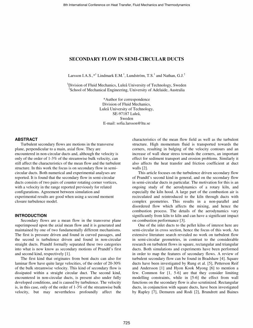
Computational Fluid Dynamic (CFD) simulations of the fully developed flow through a virtual model of a duct with an almost semi-circular cross section are performed with the commercial code ANSYS CFX 12.1. The simulations are then validated with Laser Doppler Velocimetry (LDV) measurements on the flow through a physical model built from Plexiglas with an identical geometry. The geometry, with the mesh structure, can be seen in Figure 1. Note that the mesh used for the simulations is much finer than that presented in Figure 1.

Figure 1 Geometry with mesh structure.

To achieve a fully developed velocity field, the duct has a length of 4.0 m or 95 hydraulic diameters of the semi-circular pipe both in the virtual and physical model. Dean and Bradshaw [18] obtained fully developed flow in a rectangular

duct after 93.6 hydraulic diameters for Re = 1·105 (based on the height of the duct).

Experimental setup

Secondary flows are present in the mean flow and amenable for investigation with either LDV or PIV. The advantage of PIV is the planar measurement providing directly an understanding of two dimensional flow structures [19]. The dynamic velocity range and the spatial resolution, however, are poorer than for LDV. In conjunction with a large dynamic velocity range, a large dynamic spatial range is necessary to measure small scale variation embedded in large scale motion, such as flow in boundary layers and small scale turbulence or the flow in the transverse plane in a duct. Dynamic spatial range is related to spatial resolution, and dynamic velocity range is related to the fundamental velocity resolution and accuracy of PIV [20]. Velocities yielding a displacement under 0.1 pixels between exposures are tricky to capture [21]. Raffel [22] recommends a particle displacement of ¼ of the intrerrogation area between exposures to avoid loss of particle pairs. In Larsson et al. [23] the authors studied the same setup as focused on in this work and used an interrogation area of 32

× 32 pixels with a pixel displacement of 8 pixels between exposures. This means that with a transversal velocity with the magnitude of 1-3% of the main axial velocity, the particles move 0.08-0.32 pixels in the transversal direction between exposures. It is possible to measure velocities down to 0.02 pixels with reasonable PIV algorithms. The algorithm error is fixed in pixels which means that if a maximum tolerable error is 10%, then the minimum resolvable displacement is 0.2 pixels [24]. Hence to obtain a good enough resolution of the small transversal velocity field LDV was chosen in this study.

Another main reason for using LDV instead of PIV is the optical limitation of the experimental setup. The setup is optimized to investigate the main flow in the axial direction and hence it is difficult to directly perform PIV measurements in the transversal plane.

To control the flow rate in the half circular pipe the flow was monitored with a magnetic flow meter (Krohne Optiflux DN50, error 0.1%). The temperature was monitored with a Pt100 yielding that the temperature of the water in the setup

was controlled to 22 ± 0.4 °C with a cooling system in the tank. The LDV-system used was a commercially available system

from Dantec. It is a two component setup with an 85 mm optical fibre probe and a front lens with 310 mm focal length. The system consists of a 20 W continuous wave Argon-Ion laser, transmitting optics including a beam splitter Bragg-cell, photodetectors and signal processors. The system was used in backscatter mode in combination with two Burst Spectrum Analyzers (BSA). The dimension of the measurement volume was approximately 0.074 x 0.074 x 0.63 mm for both colours when measured in air. The water was seeded with polyamide particles with a diameter of 5 µm (Dantec’s PSP-5). Dantec’s BSA Flow software with the burst mode spectrum analysis method was used for the data acquisition. The 2D-LDV probe was placed on a traversing mechanism controlled by the software, with a possible smallest step of 0.01 mm. The sampling time was set to 240 s or 900 s in each measuring point

X

Y

Z

726

for different directions of the measurements. The measurement time corresponded to at least 10000 samples depending on the location of the measuring point.

Two mass flows were investigated, 3.95 kg/s and 0.395 kg/s corresponding to Reynolds number of 8·104 and 8·103 respectively based on the hydraulic diameter. The turbulence intensity in the inlet pipe was approximately 8%.

Due to the optical limitations of the measuring section, the two secondary flow components were measured from two different directions. First, the probe was mounted facing the plane surface and the y-direction and measuring the main, axial component and the velocity in the x-direction. After that the probe was mounted beside the channel, facing the x-direction and measuring once again the main, axial velocity component and the component in the y-direction. When measuring from the side of the channel, the measurements are distorted by the optical refraction due to the curved surface of the pipe. To minimize this problem the pipe was placed in an optical measuring box filled with water.

Generally the measurement condition continuously deteriorates as the depth of the measurement volume in the test fluid increases. The worsening of the optical condition is related to the optical aberration and the dislocation of laser beam waists. This optical aberration implies that the larger the depth of the measurement volume in the flow, the fewer are the effective elementary segments on the receiving lens. This results in a deterioration of the velocity signals and thus in the decrease of the signal rate. For this reason it is unrealistic to obtain velocity signals of sufficiently high quality for depths beyond two-thirds of the pipe diameter. An entire flow distribution on a pipe diameter could only be achieved if an additional measurement is completed from the opposite side by rotating the LDV system 180° around the pipe axis [25]. Also, when traversing the laser beams towards the circular part one can exhibit “blind regions” due to the total reflection of the laser beams at the inner walls of the circular pipe. The only way to remove the blind regions, where LDV measurements cannot be performed, is to match the refractive index of the fluid to that of the tube which was judged not to be necessary in this study. In addition to the blind regions, both laser beams will have different intensities away from the pipe centre, resulting in a lower depth of modulation of the interference field, and therefore in lower values of the signal-to-noise ratio [26]. Since the four beams do not intersect in a single point due to the optical aberration of the circular surface, velocity measurements in coincidence mode were not performed when the LDV probe was mounted beside the pipe. Measurements from above the pipe were straightforward and performed in coincidence mode since the optical surface was plane.

The total uncertainty in the measurements is a combination of systematic (bias) and random (precision) errors [27]. The bias errors in LDV measurements consists of a variety of errors, such as error of the calibration factor, probe alignment/configuration bias, velocity bias and system noise. The system was carefully set up to minimize bias errors therefore the main contributors to bias errors considered in this paper are velocity bias and system noise.

In LDV measurements, the sample rate of the velocity increases with velocity. For a given observation time, higher velocities will be sampled more frequently than lower velocities. Taking a simple arithmetic mean of all samples leads to a positively biased mean compared to a true time mean of the velocity [28]. This was compensated for by weighting each velocity sample with its residence time in the measuring volume.

The system noise originates from vibrations of the test setup, leading to a small movement of the pipe wall. The system noise was estimated by a velocity measurement of the pipe wall in the measuring section, with the same hardware settings as for the flow measurements. The measured noise contribution to the velocities was subtracted from the velocity data.

The precision error was estimated by a repeatability test. Measurements at five different points were performed ten times in a randomized order. The estimated precision error (P) of the mean values, at the probability of 95% confidence interval, was calculated with the following relationship P = t · s, where t is the coefficient of the t-distribution with the corresponding degree of freedom and s is the standard deviation of the sample data [27]. The overall estimated error of the secondary velocity measurements was between 1-5%, with the higher values occurring close to the walls.

CFD setup

The geometry was imported into ANSYS ICEM and a mesh built from hexahedral elements was created. An o-grid was designed in order to get a good mesh adaptation around the curved edges. The mesh was also designed to meet the good quality mesh criterion provided by the code [29]. The overall mesh structure can be seen in Figure 1. To resolve the boundary layer, prism elements are placed close to the wall. This results in better modelling of the near-wall physics.

The turbulent flow field was solved by three dimensional, steady state, Reynolds averaged Navier-Stokes equations, closed by either the two-equation turbulence model SST or the Reynolds stress turbulence model BSL.

The SST turbulence model originates from the k-ω formulation by Wilcox [30]. The Wilcox model has the disadvantage of a strong sensitivity to free stream conditions. This can be avoided by combining the k-ω model near the surface with the k-ε model in the outer region, which is the base for the SST model. Another advantage of the SST model (compared to other hybrid models) is its capability of properly predicting the onset and amount of flow separation from smooth surfaces under adverse pressure gradients. This is due to the fact that the model accounts for transport of turbulent shear stress by introducing an eddy viscosity limiter [31].

The BSL Reynolds stress model is a turbulence model which uses the ω-equation instead of the ε-equation as the scale-determining equation. One of the advantages of the k-ω formulation is the near wall treatment for low-Reynolds number computations, where it is more accurate and more robust. As the free stream sensitivity of the standard k-ω model does carry over to the Reynolds stress model, the BSL Reynolds stress model is based on the ω-equation used in the

727

BSL two-equation model (which is basically the SST model without the eddy viscosity limiter needed in order to account for the transport of the turbulent shear stress). A separate transport equation must be solved for each of the six Reynolds stress components [29].

Turbulence-induced secondary flows are driven by the difference of the normal Reynolds stresses perpendicular to the principal velocity [5]. Because of Boussinesq’s linear (isotropic) eddy-viscosity hypothesis, which does not account for turbulence anisotropy, standard two-equation models cannot reveal secondary flow [1]. This is also shown in the present study. Due to this fact the results are taken from simulations using the Reynolds stress turbulence model. Since regions close to the wall and the corners are known to influence the characteristics of secondary flow significantly, wall function formulations should be avoided [16]. This explains the choice of turbulence models used in the present study.

A plug profile is set at the inlet and at the outlet an average static pressure is employed with a relative pressure of zero Pa, averaged over the whole outlet. A second order discretization scheme is used for the advection term. The convergence criterion is RMS residuals below 10-6 [29] and therefore double precision is used. Isothermal conditions are assumed so the energy equations are not applied. The simulations are partly carried out on a 150-node PC-cluster. It has been demonstrated that the CFD-code applied on this cluster parallelize excellently [32].

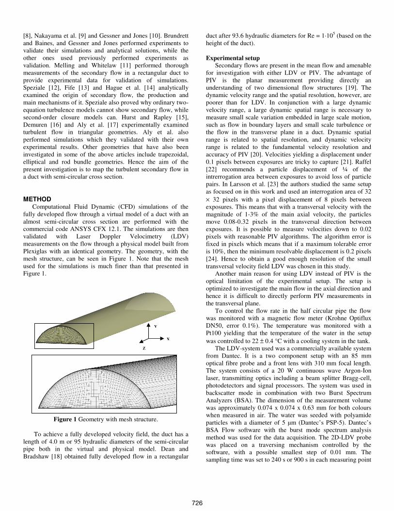
A mesh study was performed to estimate the discretization error. The dependent variable chosen to study was the efficiency factor, defined as the ratio of mass averaged total pressure at the inlet to that at the outlet [33]. Six grids were chosen where the coarsest mesh consisted of approximately 600 000 nodes while the finest mesh was built from approximately 9.6 million nodes. The Richardson extrapolation [34] was performed with a grid refinement factor of approximately 1.2. All meshes showed monotonic convergence. The calculated apparent order was 1.6 and, since a second order discretization scheme was used, the apparent order was in the right range. Agreement between the calculated apparent order and the formal order of the scheme can be taken as a good indication of the grids being in the asymptotic range. This can be seen in Figure 2. Discrepancies between the calculated apparent order and the formal order of the scheme may be due to grid quality, numerical models and boundary conditions. These things, among others, affect the calculated apparent order resulting in a lower order compared to the formal scheme. After the extrapolation was done simulations on a finer mesh consisting of approximately 16 million nodes were performed in order to confirm the extrapolated value. This point is marked with a circle instead of a star and as can be seen in Figure 2 it fits in the asymptotic region.

Figure 2 Richardson extrapolation of the efficiency factor. The circle indicates the mesh used for the simulations.

The approximate relative error for the two finest meshes

used in the extrapolation was 0.2%, the extrapolated relative error was 0.05% and the fine-grid convergence index was 0.25%. The extrapolated value of the efficiency factor, corresponding to a mesh with an infinite number of nodes, was 2.602.

The simulation results reported below are from the mesh consisting of 16 million nodes. The y+ values are in the range of 0.005 to 1.3, with an area averaged maximum value of 0.38. The maximum y+ value of 1.3 is only located just in the inlet region so the boundary layer is fully resolved everywhere throughout the geometry according to the requirements of low-Re wall formulations for an ω-based turbulence model [29]. This means that there are no wall functions to impair the prediction of the secondary flow.

RESULTS AND DISCUSSION

Due to the complexity of the measurements through the curved surface of the pipe, the errors in measuring the y-component of the secondary flow are greater than those in the x-direction. The focus is therefore on comparing the x-component of the simulation and experimental results. If not stated otherwise the simulation results are presented for the BSL Reynolds stress turbulence model.

The first indication of the existence of secondary flow is distortion of the axial flow contours, flow in the z-direction. If secondary flows are present, the axial contours will bulge out towards the corners, as can be seen in Figure 3 for the simulation result and in Figure 4 for the experimental result.

Helical streamlines of the axial flow is another indication of secondary flow. Figure 3 also shows the streamlines along the duct for the simulation results. Notice that for the SST turbulence model the streamlines are straight.

728

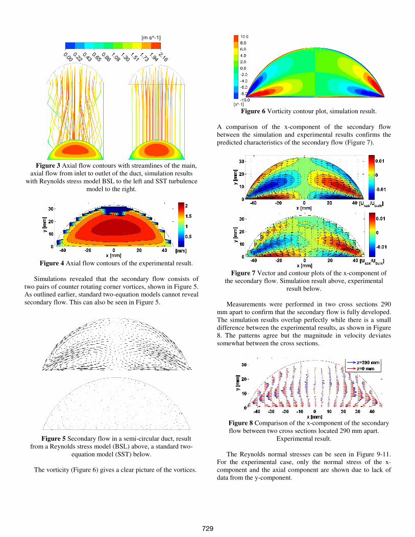
Figure 3 Axial flow contours with streamlines of the main,

axial flow from inlet to outlet of the duct, simulation results with Reynolds stress model BSL to the left and SST turbulence

model to the right.

Figure 4 Axial flow contours of the experimental result.

Simulations revealed that the secondary flow consists of

two pairs of counter rotating corner vortices, shown in Figure 5. As outlined earlier, standard two-equation models cannot reveal secondary flow. This can also be seen in Figure 5.

Figure 5 Secondary flow in a semi-circular duct, result

from a Reynolds stress model (BSL) above, a standard two-equation model (SST) below.

The vorticity (Figure 6) gives a clear picture of the vortices.

Figure 6 Vorticity contour plot, simulation result.

A comparison of the x-component of the secondary flow between the simulation and experimental results confirms the predicted characteristics of the secondary flow (Figure 7).

Figure 7 Vector and contour plots of the x-component of

the secondary flow. Simulation result above, experimental result below.

Measurements were performed in two cross sections 290

mm apart to confirm that the secondary flow is fully developed. The simulation results overlap perfectly while there is a small difference between the experimental results, as shown in Figure 8. The patterns agree but the magnitude in velocity deviates somewhat between the cross sections.

Figure 8 Comparison of the x-component of the secondary flow between two cross sections located 290 mm apart.

Experimental result.

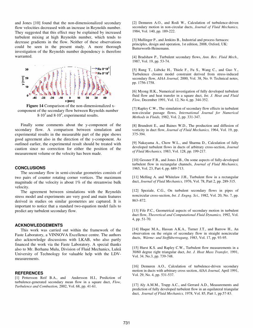
The Reynolds normal stresses can be seen in Figure 9-11. For the experimental case, only the normal stress of the x- component and the axial component are shown due to lack of data from the y-component.

729

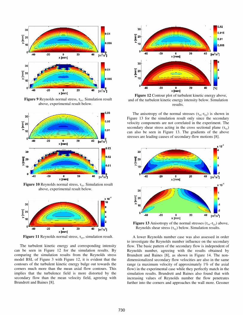
Figure 9 Reynolds normal stress, τxx. Simulation result

above, experimental result below.

Figure 10 Reynolds normal stress, τzz. Simulation result

above, experimental result below.

Figure 11 Reynolds normal stress, τyy, simulation result.

The turbulent kinetic energy and corresponding intensity

can be seen in Figure 12 for the simulation results. By comparing the simulation results from the Reynolds stress model BSL of Figure 3 with Figure 12, it is evident that the contours of the turbulent kinetic energy bulge out towards the corners much more than the mean axial flow contours. This implies that the turbulence field is more distorted by the secondary flow than the mean velocity field, agreeing with Brundrett and Baines [8].

Figure 12 Contour plot of turbulent kinetic energy above,

and of the turbulent kinetic energy intensity below. Simulation results.

The anisotropy of the normal stresses (τxx-τyy) is shown in

Figure 13 for the simulation result only since the secondary velocity components are not correlated in the experiment. The secondary shear stress acting in the cross sectional plane (τxy) can also be seen in Figure 13. The gradients of the above stresses are leading causes of secondary-flow motions [8].

Figure 13 Anisotropy of the normal stresses (τxx-τyy) above,

Reynolds shear stress (τxy) below. Simulation results. A lower Reynolds number case was also assessed in order

to investigate the Reynolds number influence on the secondary flow. The basic pattern of the secondary flow is independent of Reynolds number, agreeing with the results obtained by Brundrett and Baines [8], as shown in Figure 14. The non-dimensionalized secondary flow velocities are also in the same range (a maximum velocity of approximately 1% of the axial flow) in the experimental case while they perfectly match in the simulation results. Brundrett and Baines also found that with increasing values of Reynolds number the flow penetrates further into the corners and approaches the wall more. Gessner

730

and Jones [10] found that the non-dimensionalized secondary flow velocities decreased with an increase in Reynolds number. They suggested that this effect may be explained by increased turbulent mixing at high Reynolds number, which tends to decrease gradients in the flow. Neither of these observations could be seen in the present study. A more thorough investigation of the Reynolds number dependency is therefore warranted.

Figure 14 Comparison of the non-dimensionalized x-

component of the secondary flow between Reynolds number 8·103 and 8·104, experimental results.

Finally some comments about the y-component of the

secondary flow. A comparison between simulation and experimental results in the measurable part of the pipe shows good agreement also in the direction of the y-component. As outlined earlier, the experimental result should be treated with caution since no correction for either the position of the measurement volume or the velocity has been made.

CONCLUSIONS

The secondary flow in semi-circular geometries consists of two pairs of counter rotating corner vortices. The maximum magnitude of the velocity is about 1% of the streamwise bulk velocity.

The agreement between simulations with the Reynolds stress model and experiments are very good and main features derived in studies on similar geometries are captured. It is important to notice that a standard two-equation model fails to predict any turbulent secondary flow.

ACKNOWLEDGEMENTS

This work was carried out within the framework of the Faste Laboratory, a VINNOVA Excellence centre. The authors also acknowledge discussions with LKAB, who also partly financed the work via the Faste Laboratory. A special thanks also to Mr. Berhanu Mulu, Division of Fluid Mechanics, Luleå University of Technology for valuable help with the LDV- measurements.

REFERENCES

[1] Pettersson Reif B.A., and Andersson H.I., Prediction of turbulence-generated secondary mean flow in a square duct, Flow,

Turbulence and Combustion, 2002, Vol. 68, pp. 41-61.

[2] Demuren A.O., and Rodi W., Calculation of turbulence-driven secondary motion in non-circular ducts, Journal of Fluid Mechanics, 1984, Vol. 140, pp. 189-222. [3] Mullinger P., and Jenkins B., Industrial and process furnaces: principles, design and operation, 1st edition, 2008, Oxford, UK: Butterworth-Heinemann. [4] Bradshaw P., Turbulent secondary flows, Ann. Rev. Fluid Mech., 1987, Vol. 19, pp. 53-74. [5] Rung T., Lübcke H., Thiele F., Fu S., Wang C., and Guo Y., Turbulence closure model constraint derived from stress-induced secondary flow, AIAA Journal, 2000, Vol. 38, No. 9: Technical notes, pp. 1756-1758. [6] Myong H.K., Numerical investigation of fully developed turbulent fluid flow and heat transfer in a square duct, Int. J. Heat and Fluid

Flow, December 1991, Vol. 12, No 4, pp. 344-352. [7] Rapley C.W., The simulation of secondary flow effects in turbulent non-circular passage flows, International Journal for Numerical

Methods in Fluids, 1982, Vol. 2, pp. 331-347. [8] Brundrett E., and Baines W.D., The production and diffusion of vorticity in duct flow, Journal of Fluid Mechanics, 1964, Vol. 19, pp. 375-394. [9] Nakayama A., Chow W.L., and Sharma D., Calculation of fully developed turbulent flows in ducts of arbitrary cross-section, Journal

of Fluid Mechanics, 1983, Vol. 128, pp. 199-217. [10] Gessner F.B., and Jones J.B., On some aspects of fully-developed turbulent flow in rectangular channels, Journal of Fluid Mechanics, 1965, Vol. 23, Part 4, pp. 689-713. [11] Melling A. and Whitelaw J.H., Turbulent flow in a rectangular duct, Journal of Fluid Mechanics, 1976, Vol. 78, Part 2, pp. 289-315.

[12] Speziale, C.G., On turbulent secondary flows in pipes of

noncircular cross-section, Int. J. Engng. Sci., 1982, Vol. 20, No. 7, pp.

863–872.

[13] Fife P.C., Geometrical aspects of secondary motion in turbulent duct flow, Theoretical and Computational Fluid Dynamics, 1992, Vol. 4, pp. 51-70.

[14] Haque M.A., Hassan A.K.A., Turner J.T., and Barrow H., An observation on the origin of secondary flow in straight noncircular ducts, Wärme- und Stoffübertragung, 1983, Vol. 17, pp. 93-95.

[15] Hurst K.S. and Rapley C.W., Turbulent flow measurements in a 30/60 degree right triangular duct, Int. J. Heat Mass Transfer, 1991, Vol. 34. No.3, pp. 739-748.

[16] Demuren A.O., Calculation of turbulence-driven secondary motion in ducts with arbitrary cross section, AIAA Journal, April 1991, Vol. 29, No. 4, pp. 531-537.

[17] Aly A.M.M., Trupp A.C., and Gerrard A.D., Measurements and prediction of fully developed turbulent flow in an equilateral triangular duct, Journal of Fluid Mechanics, 1978, Vol. 85, Part 1, pp.57-83.

731

[18] Dean R.B., and Bradshaw P., (1976). Measurements of interacting

turbulent shear layers in a duct, Journal of Fluid Mechanics, 1976,

Vol. 78, Part 4, pp. 641-676.

[19] Hyun B.S., Balachandar R., Yu K., and Patel V.C., Assessment of PIV to measure mean velocity and turbulence in open-channel flow, Experiments in Fluids, 2003, Vol. 35, pp. 262–267. DOI: 10.1007/s00348-003-0652-7.

[20] Adrian R. J., Dynamic ranges of velocity and spatial resolution of particle image velocimetry, Meas. Sci. Technol., 1997, Vol. 8, 1393–1398.

[21] Lavoie P., Avallone G., De Gregorio F., Romano G.P., and Antonia, R.A., Spatial resolution of PIV for the measurement of turbulence. Experiments in Fluids, 2007, Vol. 43, pp. 39-51. DOI: 10.1007/s00348-007-0319-x. [22] Raffel M., Willert C., Wereley S., and Kompenhans, J., Particle image velocimetry: A practical guide, 2nd edition, 2007, Springer-Verlag, Berlin Heidelberg.

[23] Larsson I.A.S., Lindmark E.M., Lundström, T.S., Marjavaara D., and Töyrä S., Visualization of Merging Flow by Usage of PIV and CFD with Application to Grate-Kiln Induration Machines, Journal of

Applied Fluid Mechanics, Conditional acceptance, 2011

[24] Spedding G. R., and Hedenström A., PIV-based investigations of animal flight, Exp Fluids, 2009, Vol. 46, pp. 749-763. DOI: 10.1007/s00348-008-0597-y.

[25] Zhang Z., Optical guidelines and signal quality for LDA applications in circular pipes, Experiments in Fluids, 2004, Vol. 37, pp. 29-39. DOI: 10.1007/S00348-004-0781-7.

[26] Gardavský J., Hrbek J., Chára Z., and Severa M., Refraction corrections for LDA measurements in circular tubes within rectangular optical boxes, Laser Anemometry, Dantec Information No. 8, November 1989.

[27] Coleman H.W., and Steele W.G., Experimentation and uncertainty analysis for engineers, 2nd edition, 1999, John Wiley & Sons, New York.

[28] Albrecht H.-E., Borys M., Damaschke N., and Tropea C., Laser Doppler and Phase Doppler measurement techniques, 2003, Springer-Verlag, Berlin Heidelberg.

[29] Ansys CFX-Solver Theory Guide, 2009, Release 12.1, Elsevier

Academic Press.

[30] Wilcox D.C., Multiscale model for turbulent flows, In AIAA 24th

Aerospace Sciences Meeting, American Institute of Aeronautics and Astronautics, 1986.

[31] Menter F.R., Multiscale model for turbulent flows, In 24th Fluid

Dynamics Conference, American Institute of Aeronautics and Astronautics, 1993.

[32] Hellström G., Marjavaara B.D., Lundström T.S., (2007).

Redesign of a Hydraulic Turbine Draft Tube with aid of High

Performance Computing, Advances in Engineering Software, 2007,

Vol. 38 Part 5, pp. 338-344.

[33] Casey M., and Wintergerste T., Best Practice Guidelines. Special

Interest Group on “Quality and Trust in Industrial CFD”, 2000, 1st

edition.

[34] Celik, I.B., Ghia U., Roache P.J., and Freitas C.J., Procedure for estimation and reporting of uncertainty due to discretization in CFD, Journal of Fluids Engineering, 2008, Vol. 130, pp. 338-344.

732