Second kind integral equations for the ﬁrst kind ...€¦ · Second kind integral equations for...

Second kind integral equations for the first

kind Dirichlet problem of the biharmonic

equation in three dimensions

Shidong Jiang ∗, Bo Ren ∗, Paul Tsuji ∗∗, and Lexing Ying ∗ ∗ ∗

Abstract

A Fredholm second kind integral equation (SKIE) formulation is constructed for theDirichlet problem of the biharmonic equation in three dimensions. A fast numericalalgorithm is developed based on the constructed SKIE. Its performance is illustratedvia several numerical examples.

Key words: Second kind integral equation, Dirichlet problem, biharmonicequation.

1 Introduction

The biharmonic equations are an important class of equations in both physicsand engineering. In fluid dynamics, the so-called stream function satisfies thebiharmonic equation. Many problems in elasticity can also be formulated interms of the biharmonic equation where the fundamental physical quantitiessuch as displacement, stress, and strain all satisfy the biharmonic equation(see, for example, [30]). There have been extensive research activities on thebiharmonic equation both theoretically and computationally (see, for exam-ple, [1,9,31,32,35]). Solving the biharmonic equation numerically is a nontriv-

∗ Department of Mathematical Sciences, New Jersey Institute of TechnologyNewark, New Jersey 07102.∗∗ICES, University of Texas at Austin, Austin, TX 78712∗ ∗ ∗Department of Mathematics and ICES, University of Texas at Austin, Austin,TX 78712

Email addresses: [email protected] (Shidong Jiang), [email protected](Bo Ren), [email protected] (Paul Tsuji), [email protected](Lexing Ying).

Preprint submitted to Elsevier Science 28 March 2011

ial task. Since the biharmonic equation is a fourth order differential equa-tion, standard finite difference approximation results in a linear system withcondition number proportional to O(N4), where N is the number of the dis-cretization point in each dimension. Thus even a relatively small N causes acatastrophic loss of precision, rendering the numerical computation meaning-less. For three dimensional problems, the computational cost is prohibitive forfinite difference schemes since one has to discretize the whole domain and thestencil for the 4th order differential operator requires more than twenty pointsto achieve a good accuracy (see, for example, [2]).

In this paper, we consider the first kind Dirichlet problem of the biharmonicequation as follows. Given continuous functions f1, f2 on a sufficiently smoothsurface S in R3, find a function u ∈ C4(D) ∩ C(D) such that

∆2u = 0 on D,

u = f1 on S,

∂u∂n

= f2 on S,

(1)

where D is the domain enclosed by S. We construct a Fredholm second kindintegral equation formulation for this problem. The advantages of the SKIEformulation are obvious. First, it reduces the dimension of the problem byone since we now only need to solve integral equations with unknowns onthe boundary. Second, being a boundary integral equation formulation, it caneasily handle problems involving complex geometry. Third, for second kind in-tegral equations the condition number of the resulting linear system remainsbounded when the number of unknowns increases. Finally, there are fast nu-merical algorithms for this kind of boundary integral equations such as treecodes and fast multipole algorithms (see [6,17,18]) where the computationalcost isO(N) orO(N logN) for problems withN the total number of discretiza-tion points on the boundary. We would like to remark here that the currentlyexisting fast multipole algorithms (see for example, [6,13,14,17,18,27,36–38])either are not directly applicable to the kernels in our SKIE formulation orinvolve a large prefactor. Hence, we have developed a fast matrix-vecotr mul-tiplcation scheme based on randomized factorization for low rank matrices.The scheme is easy to implement and applicable to a broad of kernels.

There has been a great amount of work in developing numerical methods forbiharmonic equations in two dimensions. In [15], the two dimensional problemis solved by a decomposition into two Poisson problems with an iteration forthe trace of the right hand side. Since one needs to solve second order ellipticPDEs in the whole domain, the approach is not as efficient as the boundaryintegral equation method complexity-wise. The two dimensional problem hasbeen reduced to second kind integral equations by many researchers (see forexample [1,7,8,22–24,26,28,29,34]). There are also several attempts to reduce

2

the three dimensional problem to integral equations. For example in [35], the3D problem is reduced to an integral operator that is a sum of an invertibleoperator and a compact one. However, it assumes the knowledge of the LaplaceGreen’s function of a general compact domain, thus making it less convenientfor the purpose of numerical computation.

The paper is organized as follows. First, we summarize our main result inSection 2. We then present the detailed derivation of the SKIE formulation inSection 3. A numerical algorithm based on the SKIE formulation is followedin Section 4. In Section 5, we illustrate the performance (accuracy, efficiency,and robustness) of the numerical algorithm via several numerical examples.Finally, we conclude our paper with a short discussion on the extension andapplications of our method.

2 The Main Result

We use D to denote a bounded domain in R3. Its boundary, denoted by S, isassumed to be a sufficiently smooth regular surface. We use x and y to denotepoints in R3. The outward unit normal vector at a point x on S is denotedby nx. However, when the point is y, we will simply denote it by n. We user to denote the vector x− y and r to denote its length |x− y|. We use r · nto denote the dot product between r and n (note that n is boldfaced in thedot product). Finally, with a slight abuse of notation, we always use the samesymbol to denote both the kernel of an integral operator and the operatoritself.

We now summarize our main result in the following theorem.

Theorem 1 Let u be defined by the formula

u(x) =∫

S[K1(x, y)σ1(y) +K2(x, y)σ2(y)]dsy, (2)

where K1 and K2 are defined by the formulas

K1(x, y) = −2Gnnn(x, y) + 3(∆G)n(x, y) = −3(r · n)3

4πr5, (3)

K2(x, y) = −∆G(x, y) =1

4πr, (4)

with G(x, y) = − 18πr the fundamental solution of the biharmonic equation

in R3. Then u is a solution of the first (interior) Dirichlet problem of thebiharmonic equation (1) if the density σ satisfies the following system of second

3

kind integral equations:

D(x)σ(x) +∫

SK(x, y)σ(y)dsy = f(x), (5)

where

D(x) =

12

0

−H(x) 12

, σ(x) =

σ1(x)

σ2(x)

, f(x) =

f1(x)

f2(x)

, (6)

K(x, y) =

K11(x, y) K12(x, y)

K21(x, y) K22(x, y)

=

−3(r·n)3

4πr51

4πr

−9(r·n)2(n·nx)4πr5 + 15(r·n)3(r·nx)

4πr7 −r·nx

4πr3

,(7)

and H(x) is the sum of principal curvatures of S at x.

Remark 2 For exterior problems, the diagonal part D will change sign.

Remark 3 The discretized matrix D is block diagonal but non-symmetric.For certain problems, it may be advantageous that we precondition the whole

system by D−1 =

2I 0

4H 2I

.

3 Construction of the SKIE formulation

3.1 A heuristic reasoning

To reduce the first Dirichlet problem (1) to SKIEs, our strategy follows theline along Peter Farkas’ thesis [12] (we would like to remark here that [12]deals only with the two dimensional case). We try to represent the solutionvia a sum of two multiple layer potentials

u(x) =∫

S[K1(x, y)σ1(y) +K2(x, y)σ2(y)]dsy, (8)

whereKi and σi (i = 1, 2) are integral kernels (to be determined) and unknowndensities, respectively. Since u has to satisfy the biharmonic equation for x ∈D, the kernels Ki (i = 1, 2) have to be a linear combination of G and its partialderivatives. u also needs to satisfy two boundary conditions. It is well knownthat layer potentials may experience certain jumps across the boundary. Thus,

4

we denoteK11(x, y) = K1(x, y)

K12(x, y) = K2(x, y)

K21(x, y) =∂K1(x, y)

∂nx

K22(x, y) =∂K2(x, y)

∂nx

(9)

and assume that the jump relation for each associated layer potential is asfollows:

limε→0+

∫SKij(x− εnx, y)σj(y)dsy = Dijσj(x)

+∫

SKij(x, y)σj(y)dsy, x ∈ S, i, j = 1, 2,

(10)where Dij are to be determined. With this assumption, the boundary condi-tions lead to the following system of integral equations in σi (i = 1, 2)D11 D12

D21 D22

σ1(x)

σ2(x)

+

∫S

K11(x, y) K12(x, y)

K21(x, y) K22(x, y)

σ1(y)

σ2(y)

dsy =

f1(x)

f2(x)

.(11)

To make the above system second kind, we must require that the diagonal

matrix D =

D11 D12

D21 D22

has nonzero determinant and the integral operators

Kij are all compact.

3.2 Choices of K1 and K2

To simplify the discussion and fix the notation, we require further that D12 =0. Note that this can always be achieved without really changing the systemby exchanging K1 and K2 and/or forming proper linear combinations of them.Now it is easy to choose K2 such that D12 = 0, D22 6= 0 and K12, K22 areboth compact. Indeed, we may simply choose

K2(x, y) = −∆G(x, y) =1

4πr. (12)

That is, K2 is the single layer potential operator for the Laplace equation.It is well known (see, for example, [21]) that the single layer potential of theLaplace equation is continuous across the boundary (i.e., D12 = 0); its normal

5

derivative has the following jump relation:

limε→0+

∫S

∂

∂nx

1

4π|x± εnx − y|σ(y)dsy =

∫S

∂

∂nx

1

4π|x− y|σ(y)dsy∓

1

2σ(x), x ∈ S,

(13)i.e., D22 = 1

2; 1

ris only weakly singular; and ∂

∂nx

1r

is in fact continuous forsufficiently smooth boundary. Thus both K12, K22 are compact.

Remark 4 ∆G is not the only choice for K2. In fact, Gnn is another perfectlyreasonable choice which satisfies all the requirements on K2. A straightforwardcalculation shows that Gnn satisfies exactly the same jump relations as ∆G(one may also obtain this result via the standard decomposition of the Lapla-cian ∆ = ∆S +H ∂

∂n+ ∂2

∂n2 with ∆S the surface Laplacian). Indeed, one mayset K2 = −α∆G − (1 − α)Gnn for any real number α without changing thediagonal matrix D or the singular properties of K12 and K22.

Let us now try to chooseK1. SinceD12 = 0 and detD 6= 0, we must haveD11 6=0. We also require that K11 and K21 be both compact. This is a nontrivialtask. In fact, it can never be done for the Laplace equation where its doublelayer potential has a jump (i.e., D11 6= 0) and the double layer potentialoperator itself is compact (i.e., K11 is compact), but the normal derivative ofthe double layer potential is hypersingular (i.e., K21 is NOT compact). Thesituation becomes worse if one tries to use higher order layer potentials forthe Laplace equation.

Fortunately, this is not the case for the biharmonic equation. We claim thatthe following choice

K1(x, y) = −2Gnnn(x, y) + 3(∆G)n(x, y) (14)

would meet all requirements. The key is that K21 is also compact due to acancellation of the hypersingular parts. Before we continue, let us write downthe exact expressions for these kernels. We first note that by normal derivativeswe really mean that ∂f

∂n= ∇f ·n. Straightforward calculation then shows that

∂r2

∂n= −2r · n, ∂r2

∂nx

= 2r · nx,

∂r · n∂n

= −1,∂r · n∂nx

= n · nx.

(15)

6

We readily have

Gn(x, y) =r · n8πr

, Gnn(x, y) = − 1

8πr+

(r · n)2

8πr3,

Gnnn(x, y) = −3(r · n)

8πr3+

3(r · n)3

8πr5,

Gnnnnx(x, y) = −9(r · n)(r · nx)

8πr5− 3(n · nx)

8πr3

+9(r · n)2(n · nx)

8πr5− 15(r · n)3(r · nx)

8πr7,

(16)

and

∆G(x, y) = − 1

4πr, (∆G)n(x, y) = −r · n

4πr3,

(∆G)nnx(x, y) = −3(r · n)(r · nx)

4πr5− (n · nx)

4πr3.

(17)

Thus

K1(x, y) = −3(r · n)3

4πr5,

K11(x, y) = K1(x, y) = −3(r · n)3

4πr5,

K21(x, y) =∂K1(x, y)

∂nx

= −9(r · n)2(n · nx)

4πr5+

15(r · n)3(r · nx)

4πr7,

(18)

and

K2(x, y) =1

4πr,

K12(x, y) = K2(x, y) =1

4πr,

K22(x, y) =∂K2(x, y)

∂nx

= −r · nx

4πr3.

(19)

We have the following lemma.

Lemma 5 All functions Kij (i, j = 1, 2) are at most weakly singular. Henceall four associated integral operators are of order −1 and thus compact as mapsfrom Hs(S) to itself for any real number s.

PROOF. This simply follows from the well-known fact in potential theory(see, for example, [21]) that

|r · n| ≤Mr2, |r · nx| ≤Mr2, x, y ∈ S, (20)

and thus

|Kij(x, y)| ≤M

r, i, j = 1, 2 x, y ∈ S. (21)

7

3.3 Derivation of the jump relations and diagonal terms

We now derive the jump relations of layer potentials associated with K11 andK21. We assume that the density is at least twice continuously differentiable.The conventional method for deriving such jump relations relies on the globalintegral formulas like Gauss’ formula (see, for example, [21]). Here we willapply a local analysis to obtain the jump relations. The basic idea is that wewill study the asymptotic expansion of the given kernel as one point, say x,approaches the boundary. The asymptotic expansion will single out the hyper-singular terms, singular terms, terms that are approximation to the identity,and weakly singular terms. Terms that are approximation to the identity, ormore intuitively approximation to the delta function, will induce jumps acrossthe boundary. We think this local analysis approach is more natural sincethe jump relation is actually a local property. We remark here that similartechniques have already been used in [20].

For a fixed point x ∈ S, by translation and rotation of the coordinate system,we can assume that x = (0, 0, 0) and nx = (0, 0,−1). It is well known thatlocally S is the graph of a smooth function defined on the tangent space TxS.Moreover, at a small neighborhood of x, the points on S have the followingparameterization:

y = (u, φ(u)) =

(u1, u2,

1

2

n∑i=1

kiu2i +O

(|u|3

)), (22)

where k1, k2 are the principle curvatures of S at x = 0. We now consider theasymptotic expansions of K11(x+ εnx, y) and K21(x+ εnx, y) as ε→ 0 and y

is close to x = 0. We denote r = x+ εnx − y, r = |r|, and d =√u2

1 + u22 + ε2.

We have

r2 = |x+ εnx − y|2 = |u|2 + (φ+ ε)2

= d2

[1 +

ε∑2

i=1 kiu2i

d2+O

(d2)],

1

rj=

1

dj

[1− j

2

ε∑2

i=1 kiu2i

d2+O

(d2)],

n = ny =(∇φ,−1)√1 + |∇φ|2

= (k1u1, k2u2,−1)(1 +O(d2)),

(r · n)j = εj − j

2εj−1

2∑i=1

kiu2i +O(dj+2),

r · nx = ε+1

2

2∑i=1

kiu2i +O(d3),

n · nx = 1 +O(d2).

(23)

8

Using these formulas, we obtain

K11(x+ εnx, y) =3ε3

4πd5+O(

1

d), (24)

and

K21(x+ εnx, y) = − 9ε2

4πd5+

15ε4

4πd7+

9ε∑2

i=1 kiu2i

4πd5

+15ε3∑2

i=1 kiu2i

8πd7− 105ε5∑2

i=1 kiu2i

8πd9+O(

1

d).

(25)

A simple calculation using polar coordinates shows that

∫R2

1

(u21 + u2

2 + 1)5/2du1du2 =

2π

3,∫

R2

1

(u21 + u2

2 + 1)7/2du1du2 =

2π

5,∫

R2

u2i

(u21 + u2

2 + 1)5/2du1du2 =

2π

3, i = 1, 2,∫

R2

u2i

(u21 + u2

2 + 1)7/2du1du2 =

2π

15, i = 1, 2,∫

R2

u2i

(u21 + u2

2 + 1)9/2du1du2 =

2π

35, i = 1, 2.

(26)

We observe now that the kernels 3ε3

2πd5 ,3εu2

i

2πd5 , ,15ε3u2

i

2πd7 , and35ε5u2

i

2πd9 on the right sides

of (24) and (25) are all functions of the form 1ε2ψ

(uε

)with ψ a positive inte-

grable function which integrates to 1 in the parameter plane. By Theorem 1.25on page 13 of [33], the corresponding integral operators are all approximationsto the identity operator (see p.13 in [33]). Thus, we have

limε→0+

∫S∩Bδ(x)

3ε3

4πd5σ(y)dsy =

1

2σ(x),

limε→0+

∫S∩Bδ(x)

9εu2i

4πd5σ(y)dsy =

3

2σ(x),

limε→0+

∫S∩Bδ(x)

15ε3u2i

8πd7σ(y)dsy =

1

4σ(x),

limε→0+

∫S∩Bδ(x)

−105ε5u2i

8πd9σ(y)dsy = −3

4σ(x),

(27)

where Bδ(x) is a ball centered around x of sufficiently small radius δ.

Second, the first two terms on the right side of (25) are hypersingular. Using

9

(26) again we see that

limε→0

∫S∩Bδ(x)

(− 9ε2

4πd5+

15ε4

4πd7

)σ0du = 0, (28)

that is, the two terms cancel out for a constant density when taking the limit ofε→ 0. Now for a twice continuously differentiable density, we may use Taylor’stheorem to expand the density (multiplying with the Jacobian) as the sum ofa constant term, a linear term, and a second order term. The constant termvanishes in the limit process due to cancellation. The linear term vanishesdue to symmetry. And the second order term vanishes in the limit process bythe dominated convergence theorem since the whole integrand is only weaklysingular and thus integrable. Hence, the first two hypersingular terms exactlycancel out in the limit process, and we have

limε→0

∫S∩Bδ(x)

(− 9ε2

4πd5+

15ε4

4πd7

)σ(y)dsy = 0. (29)

Finally, combining (24)-(29), we obtain the following jump relations:

limε→0+

∫SK11(x± εnx, y)σ(y)dsy =

∫SK11(x, y)σ(y)dsy ∓

1

2σ(x),

limε→0+

∫SK21(x± εnx, y)σ(y)dsy =

∫SK21(x, y)σ(y)dsy ±H(x)σ(x),

(30)

where H = k1 + k2 is the mean curvature at x ∈ S.

4 Numerical Algorithm

4.1 Discretization

For a given mesh size h, we assume that the surface S is discretized with acurvilinear triangle mesh with patches Pj with diameters of order O(h), i.e.S =

⋃j∈J Pj where J serves as the index set of the patches. Each patch Pj is

parameterized by a C2 function mj : T → Pj from the standard flat triangleT . Let us define the three vertices of T by t0, t1 and t2. We denote the verticesof the mesh by xii∈I where I is the index set of vertices and write xi ∈ Pj

when xi is a vertex of the patch Pj. The value of h controls the resolution ofthis mesh of S.

The approximation space for σ1(y) and σ2(y) is the span of the basis functionsφi(x)i∈I that are local, continuous, and piecewise linear. More precisely,the function φi(x) : S → R satisfies the following conditions: (1) φi(x) iscontinuous on S, (2) the support of φi(x) is contained in

⋃j:xi∈Pj

Pj, i.e., the

10

union of the patches that contain xi, (3) φi(xi′) = δii′ , and (4) for any jsuch that xi ∈ Pj, φi(mj(t)) : T → R is linear in T . It is clear from theserequirements that the support of each φi(x) on S has a diameter of orderO(h).

A standard collocation method looks for approximations

σ1(x) =∑i∈I

σ1,iφi(x) σ2(x) =∑i∈I

σ2,iφi(x) (31)

so that when we plug them into (5) the integral equation is satisfied exactlyat the vertices xii∈I : 1

20

−H(xi)12

σ1,i

σ2,i

+∫

S

K11(xi, y) K12(xi, y)

K21(xi, y) K22(xi, y)

∑j σ1,jφj(y)∑

j σ2,jφj(y)

dsy =

f1,i

f2,i

(32)

with f1,i = f1(xi) and f2,i = f2(xi). Since the mesh size is O(h) and piecewiselinear basis functions are used in the collocation scheme, we expect formallya quadratic convergence rate O(h2). The integrals in the collocation equation(32) cannot be evaluated explicitly in general and numerical quadrature isrequired for their calculation. As the kernels K11(x, y), K12(x, y), K21(x, y),and K22(x, y) have similar behavior at the singularity, we treat them in thesame way by considering a general form∫

SK(x, y)σ(y)dsy, (33)

with K(x, y) = K11(x, y), K12(x, y), K21(x, y), or K22(x, y), and σ(y) =∑j σ1,jφj(y) or

∑j σ2,jφj(y).

The definition of the surface mesh gives∫SK(xi, y)σ(y)dsy =

∑j∈J

∫Pj

K(xi, y)σ(y)dsy =∑j∈J

∫TK(xi,mj(t))Jj(t)σ(t)dt,

(34)where Jj(t) is the Jacobian factor of the map mj : T → Pj at t. The lastintegral can decomposed into two parts:∑

j:xi 6∈Pj

∫TK(xi,mj(t))Jj(t)σ(t)dt+

∑j:xi∈Pj

∫TK(xi,mj(t))Jj(t)σ(t)dt. (35)

In the first sum of (35), since xi 6∈ Pj, the kernel K(xi,mj(t)) is never singular.These integrals over T are discretized using the standard symmetric Gaussianquadrature weights over the triangle T . Denote tα and wα to be thequadrature points and weights, respectively. The first non-singular integralthen becomes ∑

j:xi 6∈Pj

∑α

K(xi,mj(tα))Jj(tα)σ(tα)wα. (36)

11

Next, let us consider next the second sum in (35) and fix a j with xi ∈ Pj. Sincexi ∈ Pj, there exists cij with value 0, 1,or 2 such that xi = mj(t

cij). As a result,the integral

∫T K(mj(t

cij),mj(t))Jj(t)σ(t)dt can have a 1/r type singularity attcij . The Duffy quadrature [10] is used to integrate this singularity accurately.Suppose that tcβ and wc

β are the Duffy quadrature points and weights,respectively, for the vertex tc. Then the numerical quadrature form of thesecond sum in (35) is∑

j:xi∈Pj

∑β

K(mj(tcij),mj(t

cij

β ))Jj(tcij

β )σ(tcij

β )wcij

β . (37)

Once the numerical quadrature is ready, we can solve the integral equation(32). The standard method is the GMRES algorithm, which requires evaluat-ing the integral at each iteration. Therefore, from a computational viewpoint,the main task is to evaluate the two sums (36) and (37) efficiently. Let N bethe number of vertices xii∈I . For the sum (37), since xi ∈ Pj for a smallnumber of patches Pj and the number of quadrature points tcβ in the Duffyquadrature is constant, the cost of computing the second sum is proportionalto O(N). On the other hand, for the sum (36), one needs to iterate over allPj such that xi 6∈ Pj for each xi. Since there are O(N) such Pj, the directevaluation takes O(N2) steps. In order to speed up this calculation, we writeit (36) as∑

j

∑α

K(xi,mj(tα))Jj(tα)σ(tα)wα −∑

j:xi∈Pj

∑α

K(xi,mj(tα))Jj(tα)σ(tα)wα.

(38)The first sum in (38) is in fact anN -body problem with sources Jj(tα)σ(tα)wαj,α

at mj(tα)j,α, targets at xii∈I , and kernel K(x, y). An algorithm for eval-uating this N -body problem rapidly will be given in Section 4.2. As to thesecond sum in (38), since it is over j : xi ∈ Pj for each xi, the overall costis again proportional to O(N). Therefore, the algorithm for evaluating theintegral

∫S K(xi, y)σ(y)dy takes the following form:

Algorithm 1 Numerical quadrature for ui =∫K(xi, y)σ(y)dsy

1: Apply Algorithms 3 and 4 in Section 4.2 to compute

u1i =

∑j

∑α


2: For each xi, compute

u2i =

∑j:xi∈Pj

∑α


3: For each xi, compute

u3i =

∑j:xi∈Pj

∑β

K(mj(tcij),mj(t

cij

β ))Jj(tcij

β )σ(tcij

β )wcij

β .

12

4: Finally, for each xi,

ui = u1i − u2

i + u3i .

This algorithm should be repeated for four different cases for our integralequation

∫SK11(xi, y)

∑j

σ1,jφj(y)

dsy,∫

SK12(xi, y)

∑j

σ2,jφj(y)

dsy, (39)

∫SK21(xi, y)

∑j

σ1,jφj(y)

dsy,∫

SK22(xi, y)

∑j

σ2,jφj(y)

dsy. (40)

Our discretization is not optimal in terms of convergence rate. A spectrallyaccurate scheme for discretizing surface integrals can be found in [4]. However,the reason for adopting the current collocation scheme is its simplicity andflexibility to work with surfaces with singularities with edges and corners.

4.2 Fast matrix-vector multiplication

In this section, we describe the algorithm of evaluating the first integral in theprevious algorithm. In a slightly more general form, given the points pi, thenormal directions ni at pi, and the weights fi, the goal is to computefor each i

ui =∑j

K(pi, ni; pj, nj)fj. (41)

The normal directions ni are assume to depend smoothly on the points pi, i.e.,pi ≈ pj implies ni ≈ nj. Here we use K to denote the four kernels K11, K12,K21, and K22, and make their dependence on the normal direction explicit.Also, there is no distinction between the source points and target points. Inorder to compute the summations in (39) and (40), we take the point setsto be the union of the sources mj(tα)j,α and the targets xii∈I , set thefj associated to the targets to be zero, and extract the potentials ui only attargets.

We define the ε-rank rε of a matrix A of size m× n to be the number of thesingular values that are greater than ε. The matrix A is called numericallylow-rank if the ε-rank rε is much smaller compared to the dimensions of thematrix A and grows extremely slowly when ε decreases. The essential ideaof the algorithm for evaluating (41) rapidly is that, given two sets B1 andB2 well-separated ( the precise definition of well-separatedness will be given

13

later), the matrix that represents the interaction restricted to B1 and B2,

(K(pi, ni; pj, nj))pi∈B1,pj∈B2(42)

is numerically low-rank. The following randomized algorithm, first introducedin [11], constructs a low rank approximation of such a matrix in a cost that isessentially linear to the dimension of the matrix.

Algorithm 2 Randomized factorization of a numerical low-rank matrix A.

1: Select randomly a set Ω1 of γ · rε rows from the matrix A. Perform thepivoted QR factorization to A(Ω1, :). Define Π1 to be the index set thatcontains the first rε pivoted columns of A(Ω1, :). The columns of the sub-matrix A(:,Π1) then serve as a stable approximate basis for the columnspace of A.

2: Select randomly a set Ω2 of γ · rε columns from the matrix A. Performthe pivoted QR factorization to A(:,Ω2)

T . Define Π2 to be the index setthat contains the first rε pivoted columns of A(:,Ω2)

T . The rows of thesubmatrix A(Π2, :) then serve as a stable approximate basis for the rowspace of A.

3: Define the matrix M = (A(Π2,Π1))+ where (·)+ stands for the pseudo-

inverse. ThenA(:,Π1) ·M · A(Π2, :) (43)

is a rank-rε approximation of the matrix A.

This method works quite well in practice. Typically the constant γ is chosento be 3 or 4. Since rε is typically a small constant, it is not difficult to see thatthe overall cost of this algorithm is of order O(r2

ε · (m+n)) = O(m+n). Oncethis factorization is constructed, the product of A with any vector f can becomputed with

A(:,Π1) (M (A(Π2, :)f)) (44)

in O(m+ n) steps.

The algorithm for evaluating (41) consists of two stages: setup and evaluation.In the setup step, Algorithm 2 is invoked to generate the low rank factorizationfor each submatrix of form (42).

Algorithm 3 Setup stage for ui =∑

j K(pi, ni; pj, nj)fj.

1: Construct the octree structure. Starting from a square box that contains allpoints pi, we subdivided the boxes recursively into eight children boxesuntil the number of points in each leaf box is bounded by a prescribedconstant.

2: Let B be the top level box of the octree. Insert the pair (B,B) into aqueue Q.

3: Let L be an empty list.4: while Q is not empty do

14

5: Pop the top entry from Q, say (B1, B2).6: if both B1 and B2 contain points then7: if none of B1 and B2 are leaf boxes then8: if B1 and B2 are well-separated then9: Compress the matrix (K(pi, ni; pj, nj))pi∈B1,pj∈B2

using the ran-

domized procedure. Insert the triple (B1, B2, ”compressed”) intothe list L.

10: else11: Let B1,α be the children of B1 and B2,β be the children of B2.

Insert all pairs (B1,α, B2,β) into Q.12: end if13: else14: Insert the triple (B1, B2, ”dense”) into the list L.15: end if16: end if17: end while

A missing piece of the above algorithm is the definition of well-separated. Inour implementation, B1 and B2 are well-separated if the intersection of B1

and B2 is either empty or a single vertex. This criteria works quite well inpractice.

Once the setup stage is done, the evaluation stage speeds up to the matrixvector multiplication by using the constructed factorizations whenever possi-ble.

Algorithm 4 Evaluation stage for ui =∑

j K(pi, ni; pj, nj)fj.

1: for each triple of the list L do2: if the triple is of form (B1, B2, ”compressed”) then3: Evaluate the interaction between boxes B1 and B2 using the com-

pressed form4: else5: Evaluate the interaction between boxes B1 and B2 densely.6: end if7: end for

Obviously, the kernels K12 and K22 can be directly handled with the adaptivenew version FMM in [6]. It is also possible that with some modificationsthe FMM for the biharmonic equations [19] can be used for kernels K11 andK21. Furthermore, there have been many kernel-independent FMMs developedrecently (see, for example, [13,14,27,36–38]). The algorithm outlined above isessentially a tree algorithm (see, for example, [3]) with multipole expansionreplaced by randomized skeletonization (see, for example, [5]). We have chosento implement our algorithm because the algorithm is easier to implement ascompared with the FMMs, and the algorithm is directly applicable to a broader

15

class of kernels.

5 Numerical Examples

A C++ code has been written implementing the algorithm described in thepreceding section. In this section, we demonstrate the performance of thescheme with several numerical examples. We test the accuracy of our procedureby constructing a function which is biharmonic in D and setting the boundarydata equal to the function value and its normal derivative on S. Since Green’sfunction and its partial derivatives satisfy the biharmonic equation in D whenthe source is outside D, such function can be constructed, say, by forminga linear combination of Green’s functions (and its partial derivatives) withthe sources randomly distributed outside the computational domain D. Theaccuracy and speed of our algorithm depend on several parameters. In thetables below, we set the precision of the fast matrix-vector algorithm to 1e−6,the error tolerance of GMRES to 1e − 6. We choose the degree of Gaussianquadrature for smooth integrals to be 5 and the degree of the Duffy quadraturefor the weakly singular integral to be 5, so that the quadrature error from thetriangular Gaussian quadrature and the Duffy quadrature is always smallerthan the discretization error of the collocation method (32) in the followingtests.

In each of those tables, the first column contains the total number of unknownsN of the whole linear system, which is twice the total number of vertices inthe triangulation of the boundary surface. The second column contains thesetup time of the randomized matrix compression. The third column containsthe total time for solving the linear system. The fourth column contains thenumber of iterations of GMRES. The last column contains the relative L2

error of the numerical solution as compared with the analytic solution of theoriginal BVP where the checking points lie on a smaller surface inside theboundary S.

The purpose of the numerical tests is two-fold. Firstly, the numerical dis-cretization scheme presented in Section 4.1 is formally second order sincepiecewise linear basis functions are used. Therefore, if the size of the trianglesis halved (or equivalently the number of unknowns N roughly quadruples),the accuracy should decrease by a factor of four. Secondly, the fast algorithmdescribed in Section 4.2 has essentially a linear complexity. Hence, each timeN quadruples, the solution time should roughly grows by the same factor. Ineach example, we start from a fairly coarse discretization to a fairly denseone. We would like to point out that, for the coarsest discretization, standarddense solvers are often faster than the iterative solvers used here. However,since the goal is to demonstrate the two scaling behaviors mentioned above,

16

all linear systems are solved using the iterative method.

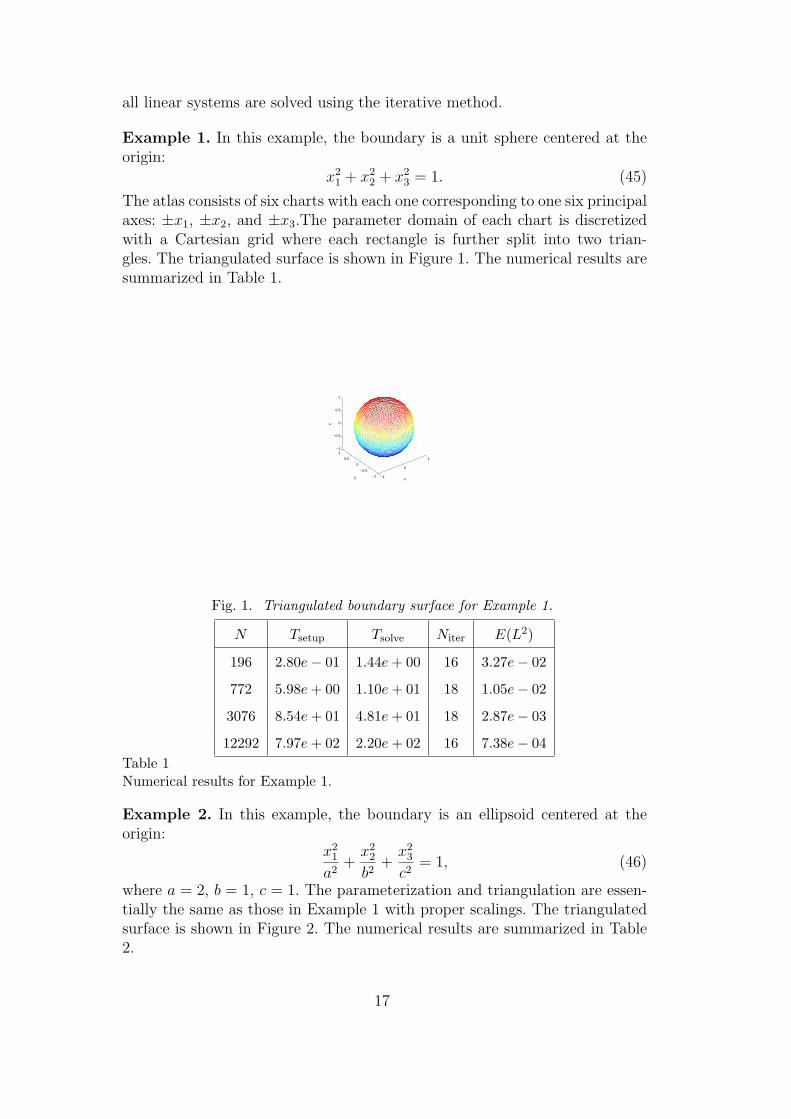
Example 1. In this example, the boundary is a unit sphere centered at theorigin:

x21 + x2

2 + x23 = 1. (45)

The atlas consists of six charts with each one corresponding to one six principalaxes: ±x1, ±x2, and ±x3.The parameter domain of each chart is discretizedwith a Cartesian grid where each rectangle is further split into two trian-gles. The triangulated surface is shown in Figure 1. The numerical results aresummarized in Table 1.

−1

0

1

−1

−0.5

0

0.5

1−1

−0.5

0

0.5

1

xy

z

Fig. 1. Triangulated boundary surface for Example 1.

N Tsetup Tsolve Niter E(L2)

196 2.80e− 01 1.44e + 00 16 3.27e− 02

772 5.98e + 00 1.10e + 01 18 1.05e− 02

3076 8.54e + 01 4.81e + 01 18 2.87e− 03

12292 7.97e + 02 2.20e + 02 16 7.38e− 04Table 1Numerical results for Example 1.

Example 2. In this example, the boundary is an ellipsoid centered at theorigin:

x21

a2+x2

2

b2+x2

3

c2= 1, (46)

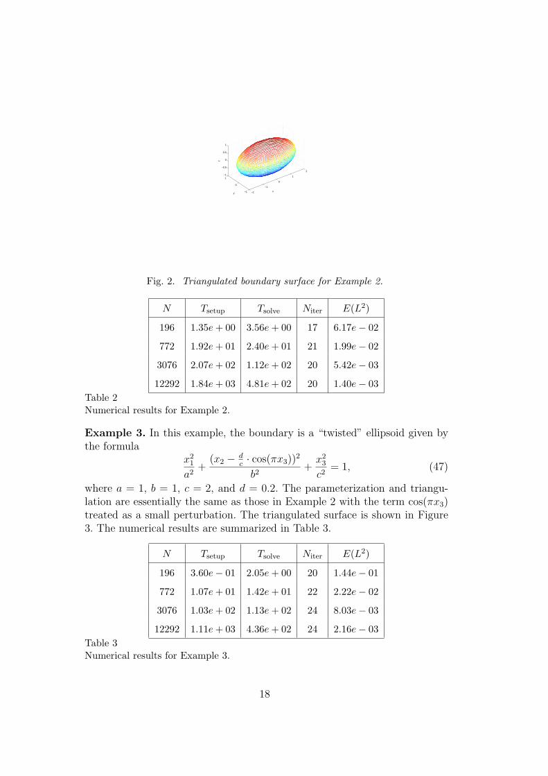
where a = 2, b = 1, c = 1. The parameterization and triangulation are essen-tially the same as those in Example 1 with proper scalings. The triangulatedsurface is shown in Figure 2. The numerical results are summarized in Table2.

17

−2

−1

0

1

2

−1

0

1−1

−0.5

0

0.5

1

xy

z



196 1.35e + 00 3.56e + 00 17 6.17e− 02

772 1.92e + 01 2.40e + 01 21 1.99e− 02

3076 2.07e + 02 1.12e + 02 20 5.42e− 03


Example 3. In this example, the boundary is a “twisted” ellipsoid given bythe formula

x21

a2+

(x2 − dc· cos(πx3))

2

b2+x2

3

c2= 1, (47)

where a = 1, b = 1, c = 2, and d = 0.2. The parameterization and triangu-lation are essentially the same as those in Example 2 with the term cos(πx3)treated as a small perturbation. The triangulated surface is shown in Figure3. The numerical results are summarized in Table 3.


196 3.60e− 01 2.05e + 00 20 1.44e− 01

772 1.07e + 01 1.42e + 01 22 2.22e− 02

3076 1.03e + 02 1.13e + 02 24 8.03e− 03


18

−1

−0.5

0

0.5

1

−0.50

0.51

−2

−1.5

−1

−0.5

0

0.5

1

1.5

2

x

y

z


Example 4. In this example, the boundary is a torus given by the formula

(√x2

1 + x22 −R)2 + x2

3 = r2, (48)

whereR = 3, r = 1. The atlas consists of a single chart with a parameterizationgiven by the formulas

x1 = (R+r·cos(θ)) cos(ψ), x2 = (R+r·cos(θ)) sin(ψ), x3 = r·sin(θ), (49)

with (θ, ψ) ∈ [−π, π)2. We then use a rectangular grid to discretize (θ, ψ)and each small rectangle is further split into two triangles. The triangulatedsurface is shown in Figure 4. The numerical results are summarized in Table4.


216 3.70e− 01 1.59e + 00 18 2.67e− 01

864 1.11e + 01 1.61e + 01 26 6.40e− 02

3456 1.40e + 02 8.78e + 01 26 2.20e− 02


In the above examples, we observe that the convergence rate is roughly equalto 2 on average, which is consistent with the convergence order of our dis-cretization scheme. The solution time Tsolve grows by a factor of 4 to 7 eachtime N quadruples. This is roughly consistent with the N logN theoreticalestimate. The fluctuations in the growth factor of Tsolve are due to various

19

−4

−2

0

2

4

−4

−2

0

2

4−1

0

1

xy

z


factors, such as the sudden change in the depth of the octree and the changesin the number of iterations of the GMRES algorithm. Most importantly, weobserve that the number of iterations is very low and roughly indepedentof total number of unknowns, which indicates that our SKIE formulation iswell-conditioned.

In our numerical examples, we triangulate the surfaces in a straightforwardmanner and compute the mean curvature at each vertex analytically. Obvi-ously, the quality of triangulation affects the accuracy greatly and in generalthe triangulation and the computation of the mean curvature should be han-dled via more general and robust algorithms available in the community offinite (or boundary) elements.

6 Conclusions and Further Discussions

We have constructed a second kind integral equation formulation for the firstDirichlet problem for the biharmonic equation in three dimensions. A fastalgorithm and a second order discretization scheme have also been developedfor solving the boundary integral equations. One may try to use this approachto construct SKIEs for other boundary value problems for the biharmonicequation. For example, the problem of finding u which satisfies

∆2u = 0 on D

∂u

∂n= f1 on S

20

∂2u

∂n2= f2 on S

for given f1 and f2, can be solved by looking for u as

u(x) =∫

S[(−2Gnn + 3∆G)(x, y)σ1(y) +Gn(x, y)σ2(y)]dsy

for which the matrix of diagonal terms is

12

0

32H(x) 1

2

.

Our construction can also be easily extended to the first Dirichlet problem forthe biharmonic equation in higher dimensions (≥ 4) and may be applicablefor solving certain boundary value problems for polyharmonic equations.

The biharmonic equation has many applications in mathematical physics.Some direct applications of the first Dirichlet problem include solving theCahn-Hillard equations for phase-transition in material science, and the phase-field models in two-phase flows (see, for example, [25]). These problems involvetime-dependent nonlinear PDEs whose principal part is a biharmonic opera-tor. The first Dirichlet conditions arise naturally in such problems since theyare the natural conditions from variational principles. We would also like to re-mark that our method can be adapted to construct the SKIEs for the modifiedbiharmonic equation, which is the governing equation of the stream functionfor unsteady Stokes flow. And an efficient numerical algorithm based on theSKIE formulation for the modified biharmonic equation will eventually lead toa numerical scheme for solving the Navier-Stokes equation (see, for example,[16]). These problems are currently under investigation and the results will bereported in a later date.

Acknowledgements

S.J. was supported in part by NSF under grant CCF-0905395 and would like tothank Prof. Leslie Greengard at Courant Institute for stimulating discussions.L.Y. was supported in part by the Sloan Foundation under a Sloan ResearchFellowship and by NSF under grant DMS-0708014 and CAREER grant DMS-0846501.

21

References

[1] S. Agmon, Multiple layer potentials and the Dirichlet problem for higher orderelliptic equations in the plane, Comm. Pure & Appl. Math. 10 (1957), 179-239.

[2] I. Altas, J. Erhel, and M. M. Gupta, High accuracy solution of three-dimensionalbiharmonic equations, Matrix iterative analysis and biorthogonality (Luminy,2000). Numer. Algorithms 29 (2002), no. 1-3, 1–19.

[3] J. Barnes and P. Hut, A hierarchical O(NlogN) force-calculation algorithm,Nature, 324 (4), December 1986.

[4] O. P. Bruno and L. A. Kunyansky, A fast, high-order algorithm for the solutionof surface scattering problems: basic implementation, tests, and applications, J.Comput. Phys. 169 (2001), no. 1, 80–110.

[5] H. Cheng, Z. Gimbutas, P. G. Martinsson, and V. Rokhlin, On the compressionof low rank matrices, SIAM J. Sci. Comput. 26 (2005), no. 4, 1389–1404.

[6] H. Cheng, L. Greengard, and V. Rokhlin, A fast adaptive multipole algorithmin three dimensions, J. Comput. Phys. 155 (1999), no. 2, 468–498.

[7] J. Cohen and J. Gosselin, The Dirichelt problem for the biharmonic equation ina C1 domain in the plane, Indiana Univ. Math. J. 32 (1983), no. 5, 635-685.

[8] J. Cohen and J. Gosselin, Adjoint boundary value problems for the biharmonicequation on C1 domains in the plane, Arkiv for Matematik 23 (1985), no. 2,217-240.

[9] M. Costabel, I. Lusikka, J. Saranen, Comparison of three boundary elementapproaches for the solution of the clamped plate problem, Boundary ElementsIX 2 (1987), 19-34.

[10] M.G. Duffy, Quadrature over a pyramid or cube of integrands with a singularityat a vertex, SIAM J. Numer. Analysis 19 (1982), 1260-1262.

[11] B. Engquist and L. Ying, A fast directional algorithm for high frequency acousticscattering in two dimensions, Communications in Mathematical Sciences, 7(2009), no. 2, 327–345.

[12] P. Farkas, Mathematical foundations for fast algorithms for the biharmonicequations, Ph.D. Thesis, University of Chicago, 1989.

[13] W. Fong, E. Darve, The black-box fast multipole method, J. Comput. Phys. 228(2009), no. 23, 8712–8725.

[14] Z. Gimbutas and V. Rokhlin, A generalized fast multipole method fornonoscillatory kernels, SIAM J. Sci. Comput. 24 (2002), no. 3, 796–817.

[15] R. Glowinski and O. Pironneau, Numerical methods for the first biharmonicequation and the two-dimensional Stokes problem, SIAM Rev. 21 (1979), no. 2,167-212.

22

[16] L. Greengard and M. C. Kropinski, An integral equation approach to theincompressible Navier-Stokes equations in two dimensions, SIAM J. Sci.Comput., 20 (1998), no. 1, 318–336.

[17] L. Greengard, V. Rokhlin, A Fast Algorithm for Particle Simulations, J. Comp.Phys. 73 (1987), no. 2, 325-348.

[18] L. Greengard and V. Rokhlin, A New Version of the Fast Multipole Method forthe Laplace Equation in Three Dimensions, Acta Numerica 6 (1997), 229–269.

[19] N. A. Gumerov and R. Duraiswami, Fast multipole method for the biharmonicequation in three dimensions, J. Comput. Phys. bf 215 (2006), no. 1, 363–383.

[20] S. Jiang, Jump Relations of the Quadruple Layer Potential on a Regular Surfacein Three Dimensions, Appl. Comput. Harmon. Anal., 21: 395-403, 2006.

[21] R. Kress, Linear Integral Equations, Second Edition, Springer, 1999.

[22] G. Lauricella, Sull’integrazione dell’equazione ∆2U = 0, Rendiconti Lincei, SerieV, Vol. XVI, 2 sem. (1907), 373-383.

[23] G. Lauricella, Sur l’integration de l’equation relative a l’equilibre des plaqueselastiques encastrees, Acta Mathematica, Vol. XXXII (1909), 201-256.

[24] G. Lauricella, Sull’integrazione dell’equazione ∆2iU = 0 per le aree piane,Rendiconti Lincei, Serie V, Vol. XVIII, 2 sem. (1909), 5-15.

[25] C. Liu and J. Shen, A phase field model for the mixture of two incompressiblefluids and its approximation by a Fourier-spectral method, Physica D 179(2003), 211–228.

[26] R. Marcolongo, La teoria delle equazioni integrali e le sue appliquazioni allaFisica-matematica, Rendiconti Lincei, Serie V, Vol. XVI, 1 sem. (1907), 742-749.

[27] P. G. Martinsson and V. Rokhlin, An accelerated kernel-independent fastmultipole method in one dimension, SIAM J. Sci. Comput. 29 (2007), no. 3,1160–1178.

[28] S. G. Mikhlin, Integral equations, Pergamon Press, New York, 1957.

[29] M. Nicolesco, Les Fonctions Polyharmoniques, Hermann et Co, Paris, 1936.

[30] A. P. S. Selvadurai, Partial differential equations in mechanics 2, Springer, 2000.

[31] J. Shen, Efficient spectral-Galerkin method. I. Direct solvers of second- andfourth-order equations using Legendre polynomials, SIAM J. Sci. Comput. 15(1994), no. 6, 1489–1505.

[32] J. Shen, Efficient spectral-Galerkin method. II. Direct solvers of second- andfourth-order equations using Chebyshev polynomials, SIAM J. Sci. Comput. 16(1995), no. 1, 74–87.

[33] E. M. Stein and G. Weiss, Introduction to Fourier analysis on Euclidean spaces,Princeton University Press, New Jersey, 1971.

23

[34] I. N. Vekua, New Methods for solving elliptic equations, John Wiley and Sons,Inc., New York, 1967.

[35] G. Verchota, The Dirichlet problem for the biharmonic equation in C1 domains,Indiana Univ. Math. J. 36 (1987), 867-895.

[36] L. Ying, A kernel independent fast multipole algorithm for radial basis functions,J. of Comput. Phys. 213 (2006), no. 2, 451-457.

[37] L. Ying, G. Biros, and D. Zorin, A kernel-independent adaptive fast multipolealgorithm in two and three dimensions, J. Comput. Phys. 196 (2004), no. 2,591–626.

[38] B. Zhang, Integral-Equation-Based Fast Algorithms and Graph-TheoreticMethods for Large-Scale Simulations, PhD thesis, University of North Carolina,Chapel Hill, 2010.

24

Second kind integral equations for the ﬁrst kind ...€¦ · Second kind integral equations for...

Documents

Transcript of Second kind integral equations for the ﬁrst kind ...€¦ · Second kind integral equations for...