Second Annual Report for Perception for Outdoor Navigation · Second Annual Report for Perception...
95
AD-A245 715 IIIl111f111iIIMIll 11l1l11l Second Annual Report for Perception for Outdoor Navigation Charles Thorpe and Takeo Kanade Principal Investigators CMU-RI-TR-91-28 DTIC ELECTE FEB11 1992' D• The Robotics Institute Carnegie Mellon University a Pittsburgh, Pennsylvania 15213 kruTh.i n sc; ~ ~uiczen -s e, _ .Pproved dit iunliited December 1991 DEENSE T C NICFI IFORMTON CNTR 9203340 © 1991 Carnegie Mellon University This report reviews progress at Carnegie Mellon from August 16, 1990 to August 15, 1991 on research sponsored by DARPA, DOD, monitored by the US Army Engineer Topographic Laboratories under contract DACA 76-89- C-0014, tided "Perception for Outdoor Navigation". Parts of this work were also supported by a Hughes Fellowship, by a grant from NSF titled "Annotated Maps for Autonomous Underwater Vehicles," and by a grant from Fujitsu Corporation. _ 2 10 092
Transcript of Second Annual Report for Perception for Outdoor Navigation · Second Annual Report for Perception...

AD-A245 715IIIl111f111iIIMIll 11l1l11l
Second Annual Report forPerception for Outdoor Navigation
Charles Thorpe and Takeo KanadePrincipal Investigators
CMU-RI-TR-91-28
DTICELECTEFEB11 1992'D•
The Robotics InstituteCarnegie Mellon University a
Pittsburgh, Pennsylvania 15213kruTh.i n sc; ~~uiczen -s e, _ .Pproveddit iunliited December 1991
DEENSE T C NICFI IFORMTON CNTR
9203340
© 1991 Carnegie Mellon University
This report reviews progress at Carnegie Mellon from August 16, 1990 to August 15, 1991 on research sponsored byDARPA, DOD, monitored by the US Army Engineer Topographic Laboratories under contract DACA 76-89-C-0014, tided "Perception for Outdoor Navigation". Parts of this work were also supported by a HughesFellowship, by a grant from NSF titled "Annotated Maps for Autonomous Underwater Vehicles," and by a grantfrom Fujitsu Corporation.
_ 2 10 092

REPORT DOCUMENTATION PAGE oM mo rove8
Public reporting burden for this -oIlectio of InformatiOn is estimated to aveae I nour per response including the time for revoewing structions, searching existing ata osorcesati..nq and maintaining the data nled, and completing and reviewing the Collection of information Send comments regarding this burden estimate or any other aspect of thiso1leti, - of information, including suggestions for reducing this Ourden to Washmqton Heaaouarters Services. Directorate for Information Oerat ns and R, orts. l 5 Jefferon
Davis High... Suite 1204. Arlington. vA 22202.4302. and to the Office of Management and Budget. Paperwork Reduction Project (0704-01U), Washington. DC 20503
1. AGENCY USE ONLY (Leave ink) PRT DATE 3. REPORT TYPE AND DATES COVERED
I Decemher 1991 I technical4. TITLE AND SUBTITLE 5. FUNDING NUMBERS
Second Annual Report for Perception for Outdoor Navigation DACA 76-89-C-0014
6. AUTHOR(S)
"/ Charles Thorpe and Takeo Kanade
7. PERFORMING ORGANIZATION NAME(S) AND ADDRESS(ES) .. PERFORMING ORGANIZATION
REPORT NUMBER
The Robotics InstituteCarnegie Mellon University CMU-RI-TR-91-28Pittsburgh, PA 15213
0. SPONSORING/ MONITORING AGENCY NAME(S) AND ADDRESS(ES) 10. SPONSORING/ MONITORINGAGENCY REPORT NUMBER
DARPA, DoD
11. SUPPLEMENTARY NOTES
12a. OISTRIBUTIONJ AVAILABILITY STATEMENT 12b. DISTRIBUTION CODE
Approved for public release;Distribution unlimited
13. ABSTRACT (Maximum 'O0worcs)
This report reviews progress at Carnegie Mellon from August 16, 1990 to August 15, 1991 on research sponsored byDARPA, DoD, monitored by the U.S. Army Engineer Topographic Laboratories under contract DACA 76-89-C-0014,tided "Perception for Outdoor Navigation."
Research supported by this contract includes perception for road following, terrain mapping for off-road navigation, andssytems software for building intcgrated mobile robots. We overview our efforts for the year, and list our publicationsand personnel, then provide further detail on several of our subprojects.
14 SUBJECT TERMS 15. NUMBER O PAGES
R'7 pp16. PRICE CODE
17. SECURITY CLASS;FICATION 18 SECURITY CLASSIFICATION 19 SECURITY CLASSIFICATION 20 LIMITATION OF ASSTRAC!iOF REPORT OF THIS PAGE OF ABSTRACT !
unlimited unlimited unlimited unlimitca

Table of Contents
1. Introduction1.1 Introduction. .. .. ... ... .... ....... .. .. .. .. .. .. .. .. ....1.2 Algorithms and Modules ..... ............ .. .........1.3 Program 4.. .. . .
1.4 Personnel. .. .. ..... .. .. ... ... .... ... .... ... ..... .. .. 51.5 Ppblications .. .. .. ... ..... . .... ... .... ... .... ... .. 5
2. 3D1 Landmark Recognition from Range Images2.1 Introduction . . . .. . . .. . . .. . . . .. . .. . .. . . . . .72. 1,1 A Scenario for Map-Based Navigation. .. .. .. ....... ... .... ...... .... 72.1.2 Sensing .. . . . . . . . . . . . . . . . . . . . . . . . . . . .2.2 Building Object Models.............. . . .... .. .. .. ... 82.2.1 Surface Models.... . .... ............. . . ., . . 92.2.2 Implementation Issues......... 92.2.3 Refining Surface Models by Merging Observations. . . . . . 122.2.4 Performance and Systems Issues..... ... . .... .. .. .. .. .. .. .. .. . ... 152.3 Finding Landmarks in Range Images. ... .. .. ... ... .... ... .... ... .. 152.3.1 Overview . .. .. . . . . . ,. . ,.,.,... . .. . .... .. 162.3.2 Initial Pose Determination. .. ... ... .... ... .... ... ... ..... 172.3.3 Pose Refinement...........................182.3.4 Performance and Extensions . ... . . . . . .. .. .. .. .. .. .. .. ... 192.4 Conclusion. . .e. .... ... .... ... .... ............. 192.5 References . 20
3. Representation and Recovery of Road Geometry In YARF3.1 Introduction .e. . .. .. .. .. .. .. .. .. .. .. .. .. .. 233.2 Techniques for recovery of road model parameters .. .. ... .... .......... 233.2.1 Methods for recovering model parameters . .......... 233.2.2 Methods for modeling road structure .*, ..- 243.3 Road model and parimeter fitting used in YARF .. . . .. .. .. .. .. .. .. .. 253.4 Errors introduced by linear approximations in YARF . .. .. .... . .~ . ., 273.4.1 Approximating a circular arc by a parabola. . ....... .: . -, 273.4.2 Translating data points perpendicular to the Y-axis 273.4.3 Evaluation of error introduced by linear approximations ., . . . . . 273.5 Parameter estimation by Least Median of Squares fitting.............. 313.5.1 Robust estimation: terminology and the LMS algorithm .. .. .. .... ... ........ 313.5.2 Examples showing the effects of contaminants on road shape estimation k. ' .. . .. "3.6 Conclusion.,. ... .. . .. ....... .. .. ........ I.I . . .,", 32
4. A Computatirrial Model of Driving for Autonomoui Vehicles*4.1 Introduction . ,. ,, , . . . . k . ,. 35
4.2 Related Work.. .. .............. . ,...36
4.2.1 Robots and Planners .. . . . ... ~. 364.2.2 Human Driving Models. ..... ,, . *.* 374.2.3 Ulysses . . . . . . .. . . . . ... . . .. ... 38
4.3 The Ulysses Driving Model. ..... . ., . . . . . . . . .39
4.3.1 Tactical Driving Knowledge .~ . . . . . .~* . . . . . . . 40
CONTENTS
4.3.1.1 A Two-Lane Highway ....... ... .. . ...... ... ...... . ..... 404.3.1.2 An Intersection Without Traffic .......................... . . 444.3.1.3 An Intersection with Traffic ....... ............................ . 484 3.i.4 A Multi-lane Intersection Approach . .. .... ........................ .... 544.3.1.5 A Multi-lane Road with Traffic .................. .... ..... . . . . 564.3.1.6 Traffic on Multi-lane Intersection Approaches ......... . . . 584.3.1.7 Closely spaced intersections .... ....... ...... ... .. .... ... . 604.3.2 Tactical Perception ......... ................................... 604.3.3 Other Levels ....... .............. ....................... . 624.3.3.1 Strategic Level ....................... . .. .. ........ 624.3.3.2 Operational Level ...... ........................................ 634.3.4 Summary ........ ...................... ................ 654.4 The PHAROS Traffic Simulator ............ . . . , 654.4.1 The Street Environment . ...... 664.4.2 PHAROS Driving Model e., . . 684.4.3 Simulator Features . . . .. . .. . .I . .. . .. .... ... .. .. . 694.5 Conclusions ., ... ........................... 71
5. Combining artificial neural networks and symbolic processing for autonomousrobot guidance5.1 Introduction . .. . . . , . , . . . . . . 775.2 Driving Module Architecture ...... .. . . .................. . ......... 775.3 Individual Driving Module Training And Performance ........... . .... . ...... 785.4 Symbolic Knowledge And Reasoning ..... .................... ......... 805.5 Rule-Based Driving Module Integration.,................. .. . 825.6 Analysis And Discussion .. ., 845.7 Acknowledgements . ................ ............. . 865.8 References............................, . ... , ... 86
Accesioi F'o. .
NTIS CRA,&
DIIC TABU";arinournied L. jJustification
!ByD),tD .ibi ,,) n j
A YV ,
A~
List of Figures
Figure 2.1: Range Image .... ....................................... .. . 9Figure 2.2: (a) Features Extracted from the Image of Figure 2.1; (b) Feature and Data Cluster,(c) Overhead View ............................ . ........... ..... 10Figure 2.3: Initializing Model Fitting from Feature Clusters ... ......................... 11Figure 2.4: Computation of Closest Data Point ....... .......................... 12Figure 2.5: Sequence of range images (left); Tracking of objects between images (right) .......... 13Figure 2.6: Merging Line Segments ........... 14Figure 2.7: Models Built frL . the Sequence of Figure 2.5 ............ .. :. ...... 15Figure 2.8: Geometry of 'le Pose Determination Problem . .. .. ................ . ... ,. 16Figure 2.9: Initial Pose Determination ,..., ., ,. ..................... . . . 18Figure 2.10: Pose Determination for a Single Object . . ..... ... . . 19Figure 2.11: Pose Determination for Two Objects . ,. .. . . . . 20Figure 3.1: Road representations and parameter recovery techniques used in various systems. ........ 25Figure 3.2: Road image with trackers on lane markings . ,. , .. .......... 26Figure 3.3: Reconstructed road model......................................... 26Figure 3.4: Error introduced by translating points to roar' spine parallel to the X axis ............. 28Figure 3.5: Fit error, fits done in vehicle coordinate system ,,, . . .. 29Figure 3.6: Fit error, virtual panning of data before fit ,. ,., ...... ........... 30Figure 3.7: Example LMS fit .. . . .... ... ...... . ....... . 31Figure 3.8: Led astray by the exit ramp ..... .... ............ . . .. ... 33Figure 3.9:, Comparison of least squares fit (left) and least median squares fit (ight) of data with outliers 33Figure 4.1: Example of tactical driving task: driver approaching crossroad.. e.. ... ........... 37Figure 4.2: Schematic of the Ulysses driver model ..... ,,., .: . ,. 40Figure 4.3:1 The two-lane highway scenario . ....... ............... .. . ... 41Figure 4.4: Deceleration options plotted on speed-distance graph .,. ... , . . ,., . . 42Figure 4.5: Robot speed profile (solid line) as it adjusts to a rolling road horizon. Maximum deceleration is -15.0fpsA2 , decision time interval 1.0 sec, horizon at 150 feet. The four dashed lines show, for the first four decisiontimes, the maximum-deceleration profile to the current horizon .. ,, . ...... 43Figure 4.6: Combining acceleration constraints ............................. . .. 44Figure 4.7:, An intersection without traffic; detection by tracking lanes . ............... 45Figure 4.8: Finding the corridor for a left turn..................... ......... 46Figure 4.9, Examples of acceleration constraints from road features at an intersection .. ....... 46Figure 4.10: Looking for possible traffic control devices at an intersection .. 47Figure 4.11: Traffic signal logic for intersection without traffic .. . . 47Figure 4.12: State transitions in Stop sign logic. . ... . .".,,.. . .... . . . . 48Figure 4.13:' Potential car following conditions at an intersection........ .. :.,.. . ......... 49Figure 4.14. Cars blocking an intersection. . , ., . . .. . . .. . . . 49Figure 4.15: Generation of constraints from traffic and traffic control., . ............ 50Figure 4.16: Right of Way decision process. 'R' is the robot, 'C' is the other car. . . b2Figure 4.17: Right of Way deadlock resc lution schemes . ........ .... ...... . 53Figure 4.18: Changes in the Wait state at an intersection .,. ........... .54
Figure 4.19: Robot observation of lane positions and markings at a multiple lane intersection approach. 55Figure 4.20: Channelization acceleration constraints......., . . .. .. . 55Figure 4.21: State changes during lane changing. . , ,, .. .... ........ 56Figure 4.22: Multiple lane highway scenario ........... .. . ,.,. ,. . ... . 57

FIGURE CONTENTS
Figure 4.23' Traffic objects that affect lane changing decisions ......................... .58Figure 4.24: Decisions at a multiple lane intersection approach with traffic..................60Figure 4.25: Visual search through multiple intersections. ......................... 62Figure 4.26: Searching for a car approaching a downstream intersection from the right. ... ........ 63Figure 4.27: Ulysses control of a vehicle in PHAROS ................. ............ 66Figure 4.28: Examples of traffic object encodings.., . . ,, . , . .......... . , , . . 67Figure 4.29: Structure of street objects ....... ............................ .. 68Figure 4.30: Example of signal head encoding in PHAROS data file................. . .,., . 69Figure 4.31: The output display of PHAROS ................ .. .. ........... 70Figure 5.1: The architecture for an individual ALVINN driving module ... ............ . ,. 78Figure 5.2: The single original video image is shifted and rotated to create multiple training exemplars in which thevehicle appears to be at a different locations relative to the road .... ...................... 78Figure 5.3: Video images taken on three of the roads ALVINN modules have been trained to handle. They are,from left to right, a single-lane dirt access road, a single-lane paved bicycle path, and a lined two-lanehighway . . ,. , . .. ... ... . -, , ............ , , , . , 79Figure 5.4.- Images taken of a scene using the three sensor modalities the system employs as input. From left toright they are a video image, a laser range finder image and a laser reflectance image. Obstacles like trees appear asdiscontinuities in laser range images. The road and the grass reflect different amounts of laser light, making themdistinguishable in laser reflectance images. ., ........ , ........... ,-, ., , - 80Figure 5.5: The components of the annotated map system and the interaction between them. The annotated mapsystem keeps track of the vehicle's position on a map. It provides the arbitrator with symbolic informationconcerning the direction to steer to follow the preplanned route and the terrain the vehicle is currently encountering.'he neural network driving modules are condensed for simplicity into a single block labeled perceptual neuralnetworks .................... . ,. ...... ......... .. . . . . .. . . 82Figure 5.6: A section of a map created and maintained by the annotated map system. The map shows the vehicletraversing an intersection between a single- and a two-lane road. The lines across the roads are alarms which aretriggered when crossed by the vehicle. Triggering an alarm results in a message being passed from the mapmanager to the arbitrator indicating a change in terrain type. The circles on the map represent the positions oflandmarks, such as trees and mailboxes. The annotated map system uses the locations of known landmarks tocorrect for vehicle positioning errors which accumulate over time ....... . ............. .. 83Figure 5.7: The integrated ALVINN architecture. The arbitrator uses the terrain information provided by theannotated map system as well as symbolic models of the driving networks' capabilities and priorities to determinethe appropriate module for controlling the vehicle in the current situation ...... ... .... 84
ANNUAL REPORT 1991
List of Tables
Table 4.1: Characteristics of three levels of driving ...... .......................... 35Table 4.2: Ulysses state variables ....... ................................ 41Table 4.3: Actions required by four classes of Traffic Control Devices . ......... . . ... . 51Table 4.4: Lane action preferences for a highway with traffic. ... . 59Table 4.5: Lane action constraints and preferences at an intersection with traffic................ 61Table 4.6: Perceptual routines in Ulysses ..... ................................ 64

ABSTRACT
AbstractThis report reviews progress at Carnegie Mellon from August 16, 1990 to August 15, 1991 on research sponsored byDARPA, DOD, monitored by the US Army Engineer Topographic Laboratories under contract DACA 76-89.C-0014, titled "Perception for Outdoor Navigation".
Research supported by this contract includes perception for road following, terrain mapping for off-road navigation,and systems software for building integrated mobile robots. We overview our efforts for the year, and list ourpublications and personnel, then provide further detail on several of our subprojects.

INTRODUCTION 1
1. Introduction
1.1 IntroductionThis report reviews progress at Carnegie Mellon from August 16, 1990 to August 15, 1991 on research sponsored
by DARPA, DOD, monitored by the US Army Engineer Topographic Laboratories under contract DACA 76-89-C-0014, titled "Perception for Outdoor Navigation".
During this second year of the contract we have made significant progress across a broad front on the problems ofcomputer vision for outdoor mobile robots. We have built new algorithms (in neural networks, range data analysis,object recognition and road finding); we have integrated our perception modules into new systems (including onroadand off road, notably on the new Navlab 11 vehicle); and we have participated in notable programmatic events,ranging from generating two new thesis proposals to playing a major role in the "Tiger Team", shaping thearchitecture for the new DARPA program in Unmanned Ground Vehicles.
This report begins with a summary of the year's activities and accomplishments, in this chapter. Chapter 2, "3-DLandmark Recognition from Range Images", provides more detail on object recognition from multiple sensorlocations. Chapter 3, "Representation and Recovery of Road Geometry in YARF", discusses geometry issues inYARF, our symbolic road tracking system. The last two chapters discuss systems issues that are important inproviding cues and constraints for an active vision approach to robot driving. "A Computational Model of Drivingfor Autonomous Vehicles", Chapter 4, introduces the complexities of reasoning for driving in traffic. The fifth andfinal chapter, "Combining artificial neural networks and symbolic processing for autonomous robot guidance",shows how we combine neural nets with map data in a complete system.
1.2 Algorithms and ModulesYARF (Yet Another Road Follower) tracks roads in color images, using specialized feature detectors to find
white lines, yellow lines, and other road markings. Individually detected features are used to update a model of roadlocation and curvature. There are several new ideas implemented in YARF this year. First, the SHIVA system nowautomatically initializes YARF by finding consistent candidate lines and edges in the first image processed.Thereafter, YARF can use known vehicle motion between frames to position feature trackers in subsequent images.
Secondly, YARF now uses robust statistics to reduce its sensitivity to errors in individual trackers. Robuststatistics methods look for consistent subsets of data, rather than always using all the data as is typical of least-squares curve fitting. Thus, a few outliers (mistakes in reported feature location) will be ignored, rather thanpossibly skewing the estimated road location. More details on the geometric reasoning of YARF, and its use ofrobust statistics, are given in Chapter 3.
Finally, YARF now has the capability to group features detected or noted as missing in multiple images. Findinga consistent gap in, for instance, a double yellow center line, is a first step in intersection detection.
SCARF, or Supervised Classification Applied to Road Following, has been reimplemented and extended.SCARF uses color clustering to derive typical colors of on- and off-road pixels in a labeled image, then uses thoseclusters to classify pixels in an unknown image as "most likely road" or "most likely non-road". The classifiedimages must them be searched to find the most probable location of the road in the image. Previousimplementations of SCARF ran in about 4 seconds per image on a Sun-4, or 2 second per image on a 10-cell Wr J.By making some simplifying assumptions, our current version runs in 0.5 seconds on a Sun-4, or 0.1 second(without I/O) on a 4 thousand processor MASSPAR. The simplifications come partly from not collecting new colorclasses for each new image, but instead using one set for as long as they are valid. The trick is to determine when

2 ANNUAL REPORT 1991
mad and off-road colors change enough that new color statistics need to be computed. We have investigated severalmethods, with promising but not yet conclusive results.
ALVINN, the Autonomous Land Vehicle In a Neural Net, continues to expand its capabilities for road following.The highlights of its performance this year include new top speed of 20 mph (which is the top speed mechanically ofthe Navlab); runs on new types of road (dirt and 4-lane paved); and driving a new vehicle (the Navlab 11, aconverted HMMWV). Technically, the biggest new thrust for ALVINN is using multiple nets to handle differentsituations. An individual network, uained for a particular type of road (say a single-lane paved road), will not beable to handle different scenes (such as a multi-lane road). Furthermore, a neural net will not usually give a goodindication of failure; instead, it will cheerfully suggest a steering direction, even if incorrect. Recent work withALVINN shows that it is possible to derive confidences for individual nets on individual scenes, and thus to selectwhich network is best for each scene. The intuition behind the approach is to use the output of a network to recreatethe expected input, and to compare the recreated input with the actual image. If the recreated input is a single-laneroad, while the actual scene is multi-lane, the images will have a large mismatch, and that network may be ignored.The subtleties of making this work have to do with appropriate weighting of each pixel.
The other continuing effort with ALVINN, detailed in Chapter 5, involves building large systems that includeboth connectionist and symbolic processing. Our approach uses a combination of cues, including map information,for vehicle positioning and guidance.
Obstacle Detection
The Navlab has been used to demonstrate computationally efficient obstacle detection using sonar and giga-hertzradar. Using an array of sonars mounted on the Navlab, the system has demonstrated stopping for obstacles;steering around obstacles; and tracking guard rails and parked cars. Each of these applications uses the sameunderlying data structure, a grid of cells in vehicle coordinates containing the location of detected objects. At eachtime step, the object locations stored in the grid are updated to account for vehicle motion. New sonar or radarreturns are then entered into the grid. A confidence is stored with each entry. If the same grid cell contains anobject for more than one time steps, its confidence increases. If an occupied grid cell does not get a new return, itsconfidence is diminished. After a user-specified interval, the confidence goes to zero, and the object is considered tohave disappeared. This gives us a primitive mechanism for handling moving objects.
Starting with the grid data structure, there are several additional processing steps used by particilar applications.The obstacle detection module calculates which grid cells the vehicle will sweep as it drives along its intendedcourse. If any of those cells are marked occupied, it decelerates the vehicle to a smooth stop before hitting theobject. Obstacle avoidance uses the same algorithm as obstacle detection, but examines several arcs, and chooses anarc that misses the obstacles. This module has been integrated with road following, to track arcs that stay near thecenter of the road while avoiding obstacles. Tracking linear objects, such as guard rails, starts by fi.ting a line to theoccupied cells that are near the vehicle's path. If the line fits the data well, and is in approxim'.tely the predictedlocation, the module has high confidence that it has correctly tracked the linear feature. It calculates the correct arcalong which to steer in order to keep the vehicle at the desired distance from the feature.
Sign Recognition
We have begun a new effort in recognizing road signs. Our first task was to hand-craft a Stop sign recognizer.We use the red color as a cue to sign location, then look for color edges, then use a variety of techniques to fit theoctagonal shape. A verification step tries to check for an appropriate number of red pixels in the detected shape,making allowance for the white lettering. The results are excellent on our small number of test samples. We will try

INTRODUCTION 3
to generalize this work to detect a variety of traffic control and caution signs. Our intent is to build a more generalprogram, rather than to hand-craft individual recognizers.
3-D Object Recognition
We have been working of building maps of the environment of a mobile robot using an laser range finder. Ourprevious work involved building maps of simple objects represented by their location and the uncertainty on theirlocation, and using the map information for navigation. We have extended the map building to build explicitthree-dimensional models of the landmarks and to use those models for navigation by matching the models withobserved object models. Including explicit shape models allows for selective landmark identification and for a moredetailed map of the environment.
The object models are built by gathering range data from several closely-spaced images. The features and datacollected on each object are used to fit a discrete surface, represented by a mesh of points, which constitutes theobject model stored in the map. This approach does not involve an explicit segmentation of the observed scene.Instead, features extracted from individual range and reflectance images are grouped in clusters corresponding toobjects in the scene. The features are range and reflectance edges and near-vertical regions. Data points that arewithin a given distance of the cluster are included as well as features. Each cluster is assumed to correspond to oneobject. Clusters are tracked from image to image using a previously developed matching algorithm. For eachobject, the surface fitting process is iterated using data and features from the previous images and from thecorresponding cluster in the new image. This leads to a refined model of each object in the scene that takes intoaccount the new data. This approach to building object models has many attractive features. Fiist, it incorporates thenatural idea of object refinement since the model is progressively refined as more data is acquired. Second, it avoidsthe problem of segmentation by going directly from only low-level features and data points to object model. Finally,it is applicable to a wide class of object shapes since it is not restricted to particular surfaces such as planar surfaces.The initial selection of objects in the image may be done automatically by identifying clusters of features, ormanually by pointing to the approximate locations of the objects. The latter may be appropriate when building a mapfor robot navigation in which only a few landmarks are relevant.
Once stored in a map, the object models can be used for navigation by using a matching algorithm. The algorithmassumes that the approximate position of the vehicle in the map is known so that the approximate location of thepredicted models in sensor space can be computed. A search through the pose space based on correlation betweenstored model and observed data gives an refined approximation of object position with respect to vehicle. Using thisapproximation as a starting point, a gradient descent yields the final estimate of the transformation between mapmodel and observed object.
We have implemented and tested those algorithms using either Navlab or Navlab II as testbed vehicles, and theErim laser range finder as sensor. The Perceptron range finder, which has better spatial resolution, was also used foroff-line experimentation only. Models of natural and man-made objects were successfully built. The models werematched with observations during vehicle travel yielding correct vehicle position. In those experiments, theperception system was tested in isolation, gathering image and position data, building and matching models withoutactually sending driving commands or position corrections to the vehicle. Our goal is now to incorporate thealgorithms in the existing Navlab navigation environment to eventually demonstrate improved mission capabilities.Sev: ,'al issues have to be addressed toward this goal. First, model building has to be performed off-line since it iscurrently very computationally demanding. Similarly, even though the time required for matching models is smallenough that t can be used while the vehicle is in continuous motion, it is currently limited to low vehicle speeds.Second, we need to identify a class of objects for which the algorithms performs best so that they can be used aslandmarks for navigition. Theoretically, the algorithms are applicable to objects representable by a single closed

4 ANNUAL REPORT 1991
surface. However, their performance vary widely depending on the characteristics of the objects. Third, we need todevelop ways to automate map building since the initial object selection is currently done manually in order to retainonly a small number of objects in the map.
Further information on 3-D data processing is found in Chapter 2.
Active Vision. We are studying active vision (control of sensors and focus of attention) in the context of "drivingmodels", used to describe perceptual behavior for driving in traffic. Driving models are needed by many researchersto improve traffic safety and to advance autonomous vehicle design. To be most useful, a driving model must statespecifically what information is needed and how it is processed. Such models am called computational because theytell exactly what computations the driving system must carry out. To date, detailed computational models haveprimarily been developed for research in robot vehicles. Other driving models are generally too vague or abstract toshow the driving processin full detail. However, the existing computational models do not address the problem ofselecting maneuvers in a dynamic traffic environment.
In our Pharos / Ulysses work we study dynamic task analysis and use it to develop a computational model ofdriving in traffic. This model has been implemented in a driving program called Ulysses as part of our researchprogram in robot vehi'le davelopmen. Ulysses shows how traffic and safety rules constrain the vehicle'sacceleration and lane ust, and shows exactly where the driver needs to look at each moment as driving decisions arebeing made. Ulysses works in a simulated environment provided by our new traffic simulator called PHAROS,which is similar in spirit to previous simulators (such as NETSIM) but far more detailed. Our new driving model isa key component for developing autonomous vehicles and intelligent driver aids that operate in traffic, and providesa new tool bc.h for traffic research and for active vision.
Details of Pharos and Ulysses are given in Chapter 4.
1.3 ProgramTheses and Proposals
During the past year, we have had two new thesis proposals, both of which should be complete within the nextyear: "Neural Network Based Perception for Mobile Robot Guidance", by Dean Pomerleau, and "YARF: A Systemfor Adaptive Navigation of Structured City Roads", by Karl Kluge. In addition, we expect the completion within thenext year of the thesis "A Tactical Control System for Robot Driving", by Douglas Reece.
Connections with other CMU programs
The work done on this contract has influenced, and been influenced by, other projects at CMU. The most obviousconnection is with the related contract "Unmanned Ground Vehicle Systems", which provides the vehicles,operations, systems architectures, and some high-speed navigation support. During the past year, the UGV contracthas built a new vehicle, the Navlab II. The Navlab II is a converted HMMWV. It has been equipped for high-speednavigation, both on and off roads. The design includes high-protection occupant seats with 4-point harnesses;suspended equipment racks for rough terrain; hard-mounted monitors; and other features for safe high-speed driving.It has driven autonomously at speeds greater than 50 mph on highways, 15 mph on dirt roads, and 6 mph onmoderate off-road terrain. Other work under that contract involves integrating perception results with a planner andcontroller that understand vehicle dynamics, for high-speed cross-country runs.
Other related projects include the NASA-sponsored AMBLER and NSF work in underwater vehicles. TheAMBLER is a 6-legged walking machine for planetary exploration. Much of the 3-D terrain mapping work is

INTRODUCTION 5
shared between AMBLER and Navlab. In addition, the AMBLER researcheis have done important work oncalibrating range scanners, which will be very useful in evaluating future sensors for Navlab. Under NSF support,we are working on two projects involving cooperation with Florida Atlantic University on underwater vehicles. Themost direct connection is in the area of underwater map building. The side-scan sonar data available underwater hassomewhat different characteristics than the 3-D data from the Navlab's scanning laser rangefinder. In particular,side-scan data is reflectance as a function of time, in a narrow vertical plane. Measuring time of reflectance givesrange in a series of concentric rings, but does not localize position along one of those rings. So converting rangedata to x, y, z points requires reasoning about surface normals from reflectance, as well as merging multiple scans.Some of these techniques are closely related to techniques and insights gained from working with laser data on theNavlab.
Finally, there continue to be strong connections with our basic Image Understanding work. In particular, newwork this past year in stereo vision and in motion analysis appear to be promising for future Navlab application.The stereo work involves multi-baseline stereo, using as many as five images on the same axis to get redundantinformation about depth. The calculations are simple and regular, so this method has good potential for parallelimplementation. The motion work, which is Carlo Tomasi's thesis, starts by finding differential motion betweendifferent points. The difference in motion between adjacent points is algebraically related to the difference in theirdepths. This method directly calculates shape (difference in depth) without first calculating depth, which givesmuch more accurate results.
Connections with other programs
The new DARPA program on Unmanned Ground Vehicles will be the framework for this Perception work. Wehave participated in the UGV workshops, including hosting the May 1991 workshop at CMU. In addition, we(Thorpe) have been involved in the Tiger Team, created by Erik Mettala to define the architecture of the UGV. TheTiger Team met during the summer of 1991 in Denver, in Monterey, again in Denver before the August UGVworkshop, and numerous times by telephone, email, and FAX.
In addition, we (Thorpe) organized the DARPA ISAT Summer Study on Autonomous Agents. This studyinvestigated the challenges and opportunities in building both physical agents, such as mobile robots, and syntheticagents, such as simulated forces in SIMNET.
1.4 PersonnelSupported by this contract or doing closely related research:
Faculty: Martial Hebert, Takeo Kanade, Chuck Thorpe
Staff: Mike Blackwell, Thad Druffel, Jim Frazier, Eric Hoffman, Ralph Hyre, Jim Moody, Bill Ross, HansThomas
Graduate students: Omead Amidi, Jill Crisman, Jennie Kay, Karl Kluge, InSo Kweon, Dean Pomerleau, DougReece, Tony Stentz
1.5 PublicationsSelected publications by members of our research group, supported by or of diroct interest to this contract.
Autonomous Navigation of Structured City Roads. D. Aubert, K. Kluge, and C. Thorpe. In Proceedings of SPIE
6 ANNUAL REPORT 1991
Mobile Robots V, 1990.
Building Object and Terrain Representation for an Autonomous Vehicle. M. Hebert. American ControlConference, June 1991.
3-D Measurements from Imaging Laser Radars. M. Hebert and E. Krotkov. IROS'91 (also accepted forpublications in IJIVC).
Neural network-based vision processing for autonomous robot guidance. D. Pomerleau. In Proceedings of SPIEConference on Aerospace Sensing, Orlando, Fl.
Rapidly Adapting Artificial Neural Networks for Autonomous Navigation. D. Pomerleau. In Advances in NeuralInformation Processing Systems 3, R.P. Lippmann, J.E. Moody, and D.S. Touretzky (ed.), Morgan Kaufmann, pp.429-435.
Combining artificial neural networks and symbolic processing for autonomous robot guidance. D. Pomerleau,J. Gowdy, and C. Thorpe. To appear in Journal of Engineering Applications of Artificial Intelligence, Chris Harris,(Ed.).
A Computational Model of Driving for Autonomous Vehicles, CMU-CS-91-122, D. Reece & S. Shafer, April1991.
Toward Autonomous Driving: The CMU Navlab. Part I: Perception. C. Thorpe, M. Hebert, T. Kanade, andS. Shafer. IEEE Expert, V 6# 4 August 1991.
Toward Autonomous Driving: The CMU Navlab. Part II: System and Architecture. C. Thorpe, M. Hebert,T. Kanade, and S. Shafer. IEEE Expert, V 6 # 4 August 1991.
Annotated Maps for Autonomous Land Vehicles. C. Thorpe and J. Gowdy. In Proceedings of DARPA ImageUnderstanding Workshop, 1990. "
UNSCARF, A Color Vision System for the Detection of Unstructured Roads. C. Thorpe and J., Crisman. InProceedings of IEEE International Conference on Robotics and Automation, 1991.
Outdoor visual navigation for autonomous robots. C. Thorpe. In Robotics and Autonomous Systems 7 (1991).

3-D LANDMARK RECOGNITION 7
2. 3-D Landmark Recognition from Range Images
2.1 IntroductionLandmark recognition is an important component of a mobile robot system. It is used to compute vehicle position
with respect to a map and to carry out a complex mission. The definition of what is a landmark varies depending onthe application, ranging from visual features, to simple objects described by their locations, to complex objects. Inthis chapter, landmarks are objects that can be represented by a closed surface. To restrict the definition, the objectsare assumed to be entirely visible in one sensor frame. This is to rule out cases in which only a small part of theobject can be visible in one sensor frame. Two issues that have to be addressed in this context. First, therepresentation of the objects must be general enough to allow for a large set of landmarks. Object models are builtfrom sequences of images. Second, finding landmark in images must be fast enough to be used while !he vehicle istraveling in continuous motion at moderate speeds.
Many different techniques may be used for modeling and recognizing landmarks. The techniques described in thischapter are based on a general map-based navigation scenario. In the remainder of this Section, the scenario isdescribed in detail in Section 2.1.1.: The sensing used in those experiments in briefly described in Secuon 2.1.2. Therest of the chapter is divided in two parts, an algorithm for building object models from sequences of range images isintroduced in Section 2.2, and an algorithm for finding landmarks in range images is described in Section 2.3..
2.1.1 A Scenario for Map-Based NavigationIn this chapter, landmark recognition is addressed in the context of map-based navigation defined as follows: A
vehicle navigates autonomously through a partially mapped environment. The map has been built through previoustraversal of the same environment. The map contains a set of landmarks, that is object models and their location inthe map. The vehicle has internal sensors that measure its approximate location and orientation. Knowing the fieldof view of the sensor, it is possible to predict which map objects may be visible from the current vehicle position.,By comparing the models with the image of the current, the position of the landmarks with respect to the vehiclemay be computed. Equivalently, the pose of the vehicle with respect to the map coordinate system may becomputed. Recognizing map landmarks as the vehicle travels can be used in two ways in this scenario: First, theestimated pose of the vehicle may be updated based on the landmarks, thus correcting for errors in the internalpositioning system of the vehicle. Second, it can be used to raise an alann when a specific landmark is reached andto take some action defined in the mission description. An example of the first case is a vehicle travelingautonomously on a road. As the distance traveled increases, the accuracy of the vehicle's internal estimate of itsposition decreases. The estimate can be reinitialized to a more accurate value, the uncertainty of which does noidepend on distance traveled. This is an example of the use of landmarks as positioning beacons. As aia example ofthe second case, let us consider a vehicle traveling through a network of roads using a road following algorithm.Assuming that the road follower is optimized for a particular type of road, it cannot handle intersections and musttherefore be turned off as it traverses an intersection. The problem is to accurately predict when the vision systemshould be turned off. This may be achieved by finding a landmark close to the intersection, correcting vehicleposition accordingly, and turning off vision as the vehicle turns in the intersection. In this example, it is critical tohave a very accurate position estimate so that the vehicle can go through the intersection relying only on deadrecloning. In general a variety of actions such as switching perception modules, adjusting vehicle speed, or stoppingmay be triggered whenever the vehicle encounters a specific landmark.
As part of the Navlab project, an initial system was built [10] in which landmarks are stored as (x,y) positions in a2-D map. The map is built through an initial traverse of the terrain. In this system, the user can specify "alarms" thatinstruct the perception system to start matching the observed objects with the stored landmarks. The matching may

8 ANNUAL REPORT 1991
be used to update the position of the vehicle by combining the current position estimate and the position estimatedfrom landmark matching [11], or to take some other action defined in the mission [11]. This first systemdemonstrated the use of landmarks extracted from range images for map-based navigation. This system used asimple representation of the objects, their (xy) location, and therefore could handle only relatively simple objectssuch as trees, mailboxes, etc. This chapter addresses the next step, that is to store a more complete description of theobjects, and to use those models for landmark recognition, so that the system can handle a larger set of objects. Thescenario and the infrastructure of the system remain the same, but it will be able to handle general environments.The next two sections describe the type of models and the techniques used for landmark recognition in this scenario,respectively.
2.1.2 SensingIn this work, object models are built using the Erim laser range finder [5)., The sensor acquires 64x256 range
images at a rate of 2 Hz. Its range resolution is 3 in from 0 to 64 ft. In addition to range, the sensor measures theintensity, generating what is sometimes called the "reflectance" image. Pixels in the range image may converted topoints in 3-D space by converting (o,0,0), p is the range, 0 the horizontal scanning angle, and 0 the vertical scanningangle, to Cartesian coordinates (xy,z) in some arbitrary reference frame fixed with respect to the sensor. In theremainder of this chapter, there is no distinction between the two representations in that a pixel in the range image isequivalent to a point in space. all the 3-D coordinates are assumed to be defined in a standard reference frameattached to the vehicle. Also, the sensor is assumed to be fixed with respect to the vehicle. Coordinates that aredescribed as being "with respert to the vehicle", "with respect to the sensor", or "with respect to the current vehicleposition" are expressed with respect to this standard reference frame.
2.2 Building Object ModelsMany object representations are possible, from parametric patches such as planes and quadrics, to complex
par.metric shapes such as superquadrics. All those representations approximate objects by a limited set ofparametric shapes. Expanding the class of allowable shapes typically requires the use of a larger number ofparameters, which yields to representations that are computationally expensive and unstable. An interesting attemptto circumvent this limitation was introduced in the TraX system in which multiple shape representations are used.Possible representations include 2-D blobs, 3-D blobs, superquadrics, generalized cylinders. The appropriaterepresentation is selected based on the amount of data available for a given object. The system switches from acoarse representation to a more detailed one whenever enough data is accumulated from consecutive images. Wealso use this idea of representation refinement but, instead of using parametric shapes, we represent objects bydiscrete surfaces that can have arbitrary shapes. Specifically, an object is represenated by a discrete mesh of nodesconnected by links. The surfaces are "free-form" in that they can theoretically represent any closed surface. The nextthree sections describe the model building algorithms and implementation in detail. First, the basic model fittingalgorithm is described in Section 2.2.1. Then, details of the actual implementation are given in Section 2.2.2. Theextension of the algorithm to building models from multiple observations is discussed in Section 2.2.3., Finally,performance and systems issues are discussed in Section 2.2.4. Thorough those sections, the emphasis is on thespecifics of the use of free-form surface models for bailding landmark models for a mobile robot. In particular,Section 2.2.2. describes the implementation issues that 'ave to be addressed in order to tailor the general approach tothis application.

3-D LANDMARK RECOGNITION 9
2.2.1 Surface ModelsGiven a set of features and data points, a surface model is built by deforming a discrete surface until it satisfies
the best compromise between three criteria: the surface should fit the data closely, it should agree with the featuresin the cluster, and it should be smooth except at a small number of discrete locations (e.g., comers)., Thiscompromise is achieved by representing the influence of features, data points, and surface smoothness by a set offorces acting on the nodes of the mesh. Forces generated by features use a spring model, i.e., proportional todistance between node and feature, so that features have an effect only when the model is far from the features.Forces generated by the data points follow a gravity model, i.e., inversely proportional to the square of the distancebetween node and data points, so that data points affect model shape only when it is close to the data. Additionalinternal forces are included to ensure overall smoothness of the resulting model. Those forces are independent offeature and data. Given those forces, the model behaves as a mechanical system composed of a set of nodes withnominal masses. The mechanical analogy gives a relation between the motion of each node and the set of forcesapplied to the node. The shape of the model is computed iteratively by moving each node at each time stepaccording to the mechanical model., The final shape is obtained after a maximum number of iterations is reached, orafter the shape does not change significantly.. The model is initialized as sphere placed near the center of the object.This approach to model fitting has many desirable properties. In particular, this definition of feature and data forcesleads to a natural model fitting sequence: Features define the overall shape during the initial iterations, while themodel is still far from the data, then data controls the local shape as the iterations proceed and the model comescloser to the data. Another important feature is that the algorithm uses directly three-dimensional data that may beexpressed relative to any arbitrary reference frame. In particular, the algorithm is not dependent on the existence of a2-D reference image coordinate system, or on a 2.1/2D surface model of the form z = f(xy). This becomes animportant consideration when data from multiple images is used, in which case there is no natural mapping between3-D data points and 2-D image points. Deformable surfaces have been used in the past to build models of curvedobject from range or intensity image data [8][12]. A complete presentation of the theory and implementation ofdeformable surfaces on which this chapter is based can be found in [3].
2.2.2 Implementation IssuesSeveral implementation issues have to be solved in order to use such a technique in this application. First, features
have to be extracted from the range and reflectance images to control the model fitting. Second, the position andradius of the sphere used to initialize the surface must be computed from image data. Such a surface should beinitialized "near" every object in the scene. Third, only part of the surface model is reliable since only part of theobject is visible. It is therefore necessary to quantify the reliability of each node on the surface model., Finally,model fitting as described in the previous section may be very expensive computationally because of the largenumber of points and featies. Solutions to each of those problems are discussed in the remainder of this section.The model fitting algorithm is illustrated by computing a model from the range image shown in Figure 2.1, This is arelatively simple case since there is a single isolated object in the scene. A more complex example involvingmultiple objects is discussed in the next section.
Figure 2.1:. Range Image
The features are currently edges in the range and reflectance images. Edges in range image are extracted using a

10 ANNUAL REPORT 1991
Canny edge detector modified to take into account the typical pattern of pixel values in a range image. Specifically,
the variation of range between adjacent pixels is greater at the top of the image than at the bottom. Therefore, thesensitivity of the edge detector varies from top to bottom of the image. Edges in the reflectance image may be due to
surface markings or to shape changes. They are also extracted using a Canny edge detector. The edges are
re ,resented by line segments. It is important to note that a complete set of edges is not needed for the model fittingto work. Only the major features of the object are needed so that the model can converge to the right shape. As a
result, conservative thresholds are used to extract edges in order to retain only the major discontinuities. In addition,
a detailed description of the graph of features is not needed, the list of line segments is sufficient. Figure 2.2 (a)show the features extracted from the image of Figure 2.1.
Figure 2.2: (a) Features Extracted from the Image of Figure 2.1; (b) Feature and Data Cluster;(c) Overhead View
To initialize the model fitting, sets of features and data points that correspond to individual objects must beextracted from the image. This is essentially a segmentation problem in that the range image must be segmented intoregions such that each region corresponds to one object. In practice, it may be hard to reliably compute an exactsegmentation. To avoid the segmentation problem, nearby features are grouped into clusters and each feature clusteris assumed to correspond to a single object. To facilitate the clustering operation, regions that correspond to slantedsurfaces are used as well as edges. The regions are extracted by grouping pixels with similar surface normals intoconnected regions. As in the case of edge features, an accurate and complete region segmentation is not needed aslong as the largest regions composing each object are found. The regions provide additional information on thelocation of potential objects since those surface are normally found on objects. They are used to facilitate thedetection of feature clusters but they are not used in the actual model fitting. A sphere of radius R. is initialized atthe center of each feature cluster and is used to start the model fitting. The data points used in the model fitting arethose within a fixed radius Rd of the center of the cluster. The geometry of model fitting initialization is summarizedin Figure 2.3. The radii R,, and Rd are nominal values determined from the average size of the objects expected in theenvironment. In the examples presented in this chapter, Rs is one meter, and Rd is three meters. Those values neednot be very accurate as long as all the data points are included in the model fitting for a typical object and as long asthe initial sphere lies within the object. Here, the only assumption is that the average size of typical objects is knownin advance. Although somewhat restrictive, this is a reasonable assumption for the current application. Thistechnique for initial object identification may generate initial clusters that do not correspond to actual objects, or itmay merge two objects into a single cluster if they are close enough. Those errors are corrected by merging multiple

3-D LANDMARK RECOGNITION 11
observations as described below. This approach to finding potential objects of interest in a range/reflectancealleviates the need for an accurate segmentation by relying on a few, easy to find, features. Figure 2.2 (b) and (c)show the region that is used for fitting a model to the object of Figure 2.1. In Figure 2.2(b), the white pixels are thedata points used in the model fitting. Figure 2.2 (c) is an overhead view of the same scene with the gey points beingthe data points used in the fitting, along with the features of Figure 2.2 (a),
'~ i tial sphere
RS RdRegion of active data points
Figure 2.3: Initializing Model Fitting from Feature Clusters
Given a cluster and the initial sphere, the model fitting proceeds as described in Section 2.2.1, The forcegenerated by an edge segment at a node of the model is computed by integrating the forces generated by the pointsof the segments over the entire segment. The 3-D coordinates of the end- points of the segment are used in thiscomputation. Similarly, the 3-D coordinates of the data points are used to compute the data force at a node of themodel surface. This involves finding the data point closest to the node, computing the distance, and thecorresponding force. The coordinates of both edge segments and data points may be expressed in any arbitraryreference frame. In the results presented in this chapter, the model surface is based on 500-point tessellation. Thisnumber of nodes is sufficient for this set of experiments, although additional work is needed to determine the bestmesh resolution for this application. The number of iterations is limited to 200.
The model fitting may be quite expensive because the distance between each node and the data points andbetween each node and the features have to be computed at each iteration in order to evaluate the external forces. Toreduce the computation time, I use the fact that the distances do not change significantly from one iteratio, to thenext if the node moves by a very small amount. In particular, the forces need not be recomputed if the position of anode differs from its previous position by an amount that is small compared to the resolution of the sensor. Inpractice, the forces, and thus the distances between node, data, and features, are recomputed only if the node hasmoved by more than 1 cm since the previous iteration. This reduces the computation time drastically towards theend of the iterations since most nodes are very close to their final positions. This test has little effect at thebeginning of the iterations since the surface tends to move faster subject to the influence of the features. During thisphase, however, most nodes are too far from the data points for the data forces to have any influence.
The next issue is that only part of the object is visible, even after merging multiple images as described in the nextSection, As a result, parts of the model correspond to region where no data is available. Clearly, those parts are lessreliable since they are smooth interpolations between parts of the model where data is available instead of beinggood approximations of the object. Therefore, model nodes in those regions should be given a smaller confidencethan in other regions. This is computed by finding the data point from the original data set that is the closest to eachnode. If such a data point exists and its distance is smaller than a threshold, the node is considered reliable,otherwise it is considered unreliable and a lower weight will be used for this node in the landmark recognitionalgorithm.

12 ANNUAL REPORT 1991
Finding the distance between dam points and model nodes can also be time consuming. The brute force approachwould consist in traversing the list of all data points for every node and find the closest ones which is obviouslyunacceptable. A more efficient approach is based on the observation that the data point closest to a node should beclose to the line L defined by the node and its surface normal. Therefore, only the set data points that are close to thisline is searched for the closest point. To minimize the amount of search, all the data points are first projected on a2-D discrete grid, then, for each model node, the line L is also projected. Finally, only the data points whoseprojection lies within a cone around the line are taken into consideration (Figure 2.4). The projection of the data setonto the grid has to be computed only once because the data is static and does change during the model fitting. Inthis application, there is a natural plane for the grid, the ground plane on which the vehicle travels. The resolutionshould be chosen so that the grid cells are small enough so that only the data within the cone of interest are searched,and Lrge enough so that the grid does not contain too many empty cells which would slow down the search. A cellotze of 20 cm realizes a good compromise in the current implementation. This implementation reduces the set ofI ta points to a small subset which makes the computation of the closest data point efficient. Instead of projectingthe data set onto a 2-D plane, it could be stored as a three-dimensional array., Theoretically, this would give betterperformance since only the data points that are inside the 3-D cone around L are taken into consideration, whereaspoints that are close in 2-D but far in 3-D may be taken into consideration in the current approach. In practice,however, a 3-D grid would be mostly empty and most of the time would be spent exploring empty space inside thecone of interest yielding worst performance than using the 2-D projection.
data points 0, 0S -- surface normal
search region
reference grid
Figure 2.4: Computation of Closest Data Point
2.2.3 Refining Surface Models by Merging ObservationsUsing data from multiple images to build a model is necessary for several reasons. First, as pointed out in the
previous section, the feature cluster approach to extracting objects from images may make occasional errors. Those
errors can be corrected only by checking the consistency of the feature clusters across images taken at differentlocations. Second, only a partial view of an object is obtained from a given viewpoint, thus yielding a partial model.
A more complete model may be obtained by merging data acquired from other locations around the object. Finally,as pointed out in [2], an initial model can and should be refined by accumulating data to yield the most accuratemodel. In this application, multiple observations are obtained by acquiring range images from vehicle positionsseparated by small distances, typically 50 cm. The requirement of small displacement is necessary to ensure that anobject is visible in a large enough number of images, and to ensure that the estimate of the displacements betweenvehicle positions are accurate enough. The merging of observations is a three-step process: identify common clusters
between images, remove incorrect clusters, and merge data and features from matched clustery

3-D LANDMARK RECOGNITION 13
Given a current set of clu.;ters, corresponding clusters in the next image are searched to find candidates formatches. The set of possible matches is traversed to find the best set of matches between the two sets of clusters.Common clusters are matctied by predicting where an existing cluster should appear in the next image. In th,3application, this can be done by using the estimate of vehicle displacement between the position for the new imageand the reference position. This estimate is quite accurate for small displacements of the vehicle from image toimage. As a result, there are typically very few possible matches, and most often only one, for each cluster, thusreducing the search fror potentially combinatorial to close to linear in most casrs. Incorrect clusters are removed bymaintaining a confidence number defined as the ratio of the number of time a cluster is matched versus the numberof time it is predicted to appear in the images. The confidence is low if the cluster does not correspond to an actualobject and therefore appears in only one, or a few, of the images of a sequence. Therefore, clusters with lowconfidence are removed while clusters with high confidence are retained.
For each cluster, the features from all the images in which it appears are grouped into a single list. Similarly, allthe data points from all the images in which the cluster appears are grouped into a single list. Once this matchingand merging of c'usters is completed, a sphere is initialized at the center of each cluster and used as a starting pointto the model fitting as described above. Figure 2.5 (left) shows a sequence of range images taken in parking lot, theobjects on the left are parked cars, Figure 2.5 (right) shows h )w the clusters conesponding to the objects are trackedbetween images. In this display, the extremities of the black and white line segments are at the center. of the clustersand join matching clusters. Three sets of clusters are correctly merged into three objects on the right side of theimages. An erroneous cluster is detected on the left side but is discarded since it is not matched consistently in thissequence. This example shows that extracting, matching, and merging clusters of features yields a good initial list efobjects from the range image even in the absence of actual segmentation of the image.
Figure 2.5: Sequence of range image (left); Tracking of objects between images (right)
One implementation issue is that simply grouping the features from several images in one list is very inefficientsince several slightly different copies of a feature may be present in the list. In addition, this would effectively give a

14 ANNUAL REPORT 1991
higher weight to duplicated features, thus introducing a bias toward this feature in the deformation process used inmodel fitting. The obvious solution is to identify common features between observations within each cluster. Sinceall the coordinates of all the features are expressed in the same coordinate frame, edge segments corresponding tothe same physical feature should be close to each other in this reference frame. A natural way to merge redundantfeatures is therefore to search the set of overlapping features to find groups of segments that are nearly collinear andthat have large overlap with each other. Segments within a group are merged into a single segment by firstcomputing the least-squares line fit to all the vertices and by projecting the vertices onto this line. The two extremaof the projections along with the line describe the resulting segment (Figure 2.6). This algorithm is based onheuristics for defining the "best" combination of features, which is sufficient for the current application. However,more rigorous algorithms based on optimal estimation should be used in the future.
segments from multiple images new endpoint
Figure 2.6: Merging Line Segments
A similar issue is that merging the sets of data points from several images into one list may lead to grosslyoversampled surfaces. For example, a surface patch that has a thousand data points measured on it would end upwith ten times that number if it is fully visible in ten successive images. Clearly, such a large amount of data isunnecessary. It slows down the model fitting dtastically, and it does not improve the resulting model. It is thereforeimportant to have a strategy to add data from new observations only when it might improve the model. One possiblestrategy is to add a data point from a new observation only if the density of existing data points in its vicinity issmall enough. The threshold on data density is relative to the resolution of the sensor, in this case three inches,because adding points in a region where the average distance between data points is much smaller than sensorresolution does not add any information. Although th3 results presented in this chapter were obtained using thisstrategy, it is not optimal because it would be better to keep the most recent measurements and discard the old onesif the density becomes igh enough, or better yet to combine data points using an optimal estimation techniquebased on the uncertainty on the measurements.
As an example, Figure 2.7 shows the set of models computed from the image sequence of Figure 2.5., The displayshows an overhead view of the set of data points and of the tessellation associated with each object. The linesegments correspond to features from the images. Only the data in the right part of the images in displayed. Sinceonly part of each object is visible, only the model nodes that are close to the data are taken into consideration lateron in the matching.
This is a "batch" approach to merging observations in that all the images in a sequence are processed first, andthen the model fitting is applied to clusters that contain data and features from all the images. A recursive approachwould be more natural: Each time a new image is available, the current object model for each cluster is mod.tiedaccording to the features and data from the new image. The recursive approach is a natural implementation of theidea of model refinement which is more efficient than the batch approach since only a few additional iterations ofmodel fitting are needed each time a new image is taken. However, it is not clear that the gain is significant sinceredundant features and data cannot be eliminated as easily using a recursive approach. Also, some of the

3.D LANDMARK RECOGNITION 15
-'..
Figure 2.7: Models Built from the Sequence of Figure 2.5
optimizations described in Section 2.2. require that all the data be available at the beginning of the model fitting.The current approach demonstrates the use of multiple observations and the model building capabilities but morework is needed to find the optimal strategy for combining multiple observations and model fitting.
2.2.4 Performance and Systems IssuesUsing free-form discrete surface has several advantages. First, it is very general since it does not rely on a
particular set of geometric primitives. Second, a given model can be refined in a natural way by simply adding newdata and iterating the surface fitting process. Third, it does not require an exact segmentation objec/background asan input, thus being able to use a crude segmentations as input. In addition, it does not take into account spuriousfeatures and data that may be included in a cluster. The main drawback of this approach is that the surface modelprovides a good approximation of the overall shape of an object but may not yield as good a local approximation asother techniques. For example, sharp surface discontinuities such as corners may be recovered best by local surfaceanalysis, whereas the method described here will tend to smooth those features.
Another issue is the computation time required by the model fitting algorithms. Building a model of a typicalobject from a sequence of ten images may take several minutes on a Sun4 workstation. This includes convertingrange pixels to 3-D coordinates, extracting features, grouping feature into clusters, merging clusters from multipleimages and doing the actual iterative model fitting. As a result, this technique can be used in a scenario in which asequence of images is first collected and then processed off-line to produce the object models, but it cannot be usedto generate models in real time as the vehicle travels, even at low speed. Currently, this is not a major limitationsinc( nost scenarios can accommodate off-line model building.
2.3 Finding Landmarks in Range ImagesIn the scenario introduced in Section 2.1.1, the object models stored in the map are i,'atch(d with observations to
correct vehicle position and to identify locations at which the vehicle must take specific actin. This problem can bestated as a pose determination problem: Find the pose of a model that is most consistent with the data in a rangeimage taken at the current vehicle position. The geometry of the problem is illustrated in Figure 2.8. A modelrepresented by a discrete surface as described in Section 2. is predicted by the navigation syst?'- to be within the

16 ANNUAL REPORT 1991
field of view of the vehicle at its current location. The problem is to find the pose -if the landmark with respect to thevehicle coordinate system defined by the six parameters P = (xy,z,9,O,,). Knowing P, the vehicle pose with respectto the map coordinate can be easily derived. If several models are predicted at once, the algorithm must be able tocompute the correct mapping between image regions and landmarks. Unlike model building which is an off-lineactivity, landmark finding must be executed on-line as the vehicle is traveling. This implies that computationalefficiency is critical in landmark finding. This is a hard problem in general but the navigation scenario of Section2.1.1. introduces constraints that make pose determination possible. In this Section, I describe the approach to posedetermination and discuss some implementation issues. Section 2.3.1 gives an overview of the algorithm in thecontext of the map-based navigation scenario. The Agorithm is divided into two parts: initial pose estimation andpose refinement which are discussed in sections 2.3.2 and 2.3.3. Performance and possible extensions of thealgorithm are discussed in Section 2.3.4.
Z cene eo"
Yscene ZapYma
Xscene iiapoestimate SXmap
Figure 2.8: Geometry of the Pose Determination Problem
2.3.1 OverviewThis recognition problem is very hard in general if there is no apriori information. In particular, it is very hard if
there is no information on the expected pose of the model in the image. Fortunately, the navigation scenariointroduces strong constraints on the problem that render the landmark recognition problem manageable. There arebasically three constraints that can be exploited. First, the objects are known to be on the same terrain on which thevehicle is traveling. Second, the position and orientation of the vehicle with respect to the reference frame in whichthe map is represented is known within some small uncertainty.. Third, the objects are static and their locations in themap is assumed to remain constant. The first constraint implies that the elevation z, and the angles 0 and y, of theobject with respect to the vehicle are very close to their values in the map. The second constraint implies that the xylocation and q orientation of the model with respect to the vehicle can be predicted within a small uncertainty. Thisis a reasonable assumption since the vehicle pose can always be estimated from other sources, such as deadreckoning and road tracking, for example. The third constraint guarantees that there is a rigid transformationbetween object in vehicle reference frame and model in map reference frame. As a result of those three constraints,only a small subset of the pose space has to be searched in order to find the best model pose. The size of pose space
is defined by the expected variation in terrain for the z, 0, and W degrees of freedom, and by the expected maximum
uncertainty in vehicle pose for the x, y, and 0 degrees of freedom. The numbers currently used are plus or minus 5degrees for 0 and xV, plus or minus 1 meter for the z component, plus or minus 3 meters for the x and y components,and plus or minus 20 degrees for the 0 coi..ponent. Those numbers are overestimates of the expected uncertainty onvehicle pose that were chosen to demonstrate the system. A detailed analysis of the actual uncertainty in the current
system is described in [10]. In the future, the actual uncertainty on vehicle pose should be used directly instead ofthose arbitrary values to make the system more efficient.

3-D LANDMARK RECOGNITION 17
Having defined the possible poses of the model with respect to the vehicle, the next step is to find the best modelpose within this space by matching the model representation with the image data. A natural way of doing thematching would be to extract object models from the image as described above, and compare them with the storedmodel. Another approach is to directly compare the stored model with the image data directly. Although the firstapproach is closer to the traditional object recognition approach, in which the same representations are used forobserved and stored models, it is more computationally expensive because of the time required to extract and buildmodels from the image. Furthermore, the pose constraints make the second approach feasible even though it wouldbe Lnpractical in the general case. Another advantage is that does not require any preprocessing of the image exceptfor some initial filtering. In particular, it does not require an exact segmentation of the scene. In this approach, thepose determination is a two.stage process. First, the pose space is discretized and a measure of similarity isevaluated for each possible pose Pi in the discretized pose space. The pose P 1""' that corresponds to maximumsimilarity is retained. This first step gives a coarse approximation of model pose. In the second step, the minimum ofthe similarity measure is found through a gradient descent in pose space, taking PImni as a starting point.
Similar approaches to pose determination have been used in other perception systems for navigation. As anexample of the initial pose determination step, in [7] landmark pose is determined by comparing the predictedappearaiice of a superquadrics model surface with a range image of a scene. As an example of the pose refinementstep, a gradient descent technique is used in [6] to minimize the distance between a stored terrain map and the terrainmap observ'ed by a laser range finder at the current vehicle position. Although based on different models and slightlydifferent scenario, those two systems contain the two major building blocks of our approach: initial posedetermination through search of pose space, and gradient descent through estimation of the derivatives of asimilarity measure with respect to pose paremeters.
2.3.2 Initial Pose DeterminationThere are two components that affect the performance of this algorithm: the resolution of the discretized pose
space, and the similarity measure. The resolution of the pose space should be coarse enough so that not too manyposes are evaluated, but it should also be fine enough so that P!
M" is close enough to the actual minimum for thesecond step to converge properly. The resolution depends also on the average size of the objects and on theresolution of the sensor. For the objects used in the currant experiments, resolutions of 0.5 m for the translationaldegrees of freedom, and 5o for the rotational degrees of freedom realize a good compromise. This involvescomputing the similarity measure at about 1800 different poses in the worst case. The similarity measure is definedas the sum of mean square distances between each node of the model and the corresponding point from the imageweighted by the surface area represented by that node. The sum is taken over the set of nodes that is predicted to bevisible in the image for a given pose. There two problems with this initial definition of the similarity measure. First,if a few image points are far from the surface the similarity measure becomes very high even though the pose maybe correct. This can happen because of occasional erroneous range measurements, or, more commonly, because panof the predicted model intersects the background in the image. This problem is solved by not including distancesthat are greater than a threshold in the summation. The threshold is again related to the expected size of the objects,or, more precisely, to the minimum distance between object point and baricground at an occluding edge. A pose isretained for further consideration if more than 50% of the expected visible area of the model is included in thesummation according to the threshold. The complete algorithm for initial pose determination is illustrated in Figure2.9.
The 50% threshold is used to reduce the computation time of the similarity measure. More precisely, thecomputation of the similarity is stopped as soon as the percentage of surface area that remains to be evaluated plusthe percentage that has already been included in the summation is lower than 50%. This stopping condition meansthat even if the computation were carried through, it would be impossible to include the minimum 50% of visible

18 ANNUAL REPORT 1991
Predicted subset
P' Jsimilarity poMi
PnK > measuremodel transformed models images current range
image
Figure 2.9: Initial Pose Determination
area, and therefore the pose would be rejected. This optimization of similarity computation speeds up the search ofpose space by a factor of two on average.
The computation of similarity for all poses would still be very expensive if model nodes had to be converted topixel pnsitions in image for every possible pose. In the actual implementation, the positions o; "' iodel nodes inthe range image are computed off-line for every pose in the discretized pose space. They are computed only onceand stored along with the model. To facilitate the computation of similarity, the expected model appearance for agiven pose is stored as an image, that is an array of points registered with the range image, by interpolating betweennodes, Similarity can then be evaluated by adding up the distances between individual points in the range .nage andpoints in the predicted image of the model. Precomputing and storing the model appearance for all the poses isclearly an improvement in terms of computation time but it may require a large amount of storage space. In practice,however, a typical model requires a thousand points per pose on average for a total size of two to three Megabyteson average. This model size is acceptable in the navigation scenario since only a small number of models may beactive and loaded in the system at a given time.
2.3.3 Pose RefinementThe initial pose P- is only a coarse approximation of the best pose since its estimation is limited by the
resolution of the pose space. A natural way of refining the pose estimate is to use a gradient descent technique tooptimize similarity, taking Pi"'im as a starting value. Since both data and model are based on a discreterepresentation, the gradient must be estimated numerically. This is done by computing the difference between thesimilarity measure at the current pose and similarity at poses obtained by varying the parameters by a small amount.Those differences are estimates of the derivatives of similarity with respect to pose parameters. The pose is updatedby moving in the direction of the gradient by a small amount. The steps used for computing the gradient and forupdating the pose are 10 cm and 0.5 degree in translation and rotation, respectively. Those two values also definethe accuracy of the resulting pose. Those numbers are larger than in other recognition systems but they reflect theresolution of the sensor and based on estimates of the best accuracy that can be reasonably expected from thissensor.
A known problem with this type of techniques is that there is a cross-talk between the translational and rotationalparts of the pose parameters. Specifically, a small AO may have the same effect on the similarity measure as a smallvariation in translation Ax. To minimize this effect, (x,y,z) and (0,0,y) are updated separately at alternatingiterations. Also, this approach could lead to local extrema in general. In this case, the starting pose p,,n is closeenough to the best pose that the algorithm converges rapidly toward the optimum., The iterations stop when thesimilarity does not improve significantly by changing the pose. In practice, only two or three iterations are necessary

3-D LANDMARK RECOGNITION 19
to find the best pose.
23.4 Performance and ExtensionsThe entire pose determination procedure takes between 100 and 500 ms on a Sparc2 workstation depending on the
model. This computation time makes it possible to use this technique to accurately locate landmarks in theenvironment while the vehicle is traveling in continuous motion at moderate speeds. The basic operations used inpose determination may be easily distributed over multiple processors since most of them are point-by-pointoperations. This would yield real-time operation of the system. Figure 2.10 shows where one of the models of Figure2.7 is found in a range image. The top image shows the superimposition of the outline of the visible part of themodel, shown as a black contour. The visible part is defined as the portion of the model that is used to evaluate thesimilarity at this pose. The bottom image show only the predicted appearance of the model. Only the part that isclose enough to the data, that is the part that contributes to the similarity measure, is shown. In this example, anartificial error of one meter in translation was introduced in the initial estimate of pose, which is corrected by thepose determination algorithm.,
Figure 2.10: Pose Determination for a Single Object
The pose determination described so far assumes that a single model is to be found in the image. In practice,however, several landmarks may be predicted to appear in the field of view of the sensor leading to ambiguousinterpretations of the scene. This situation is addressed by computing Pi/ad for, each of the predicted models, andverifying that the resulting set of poses is consistent with the relative positions of the models in the map. Figure 2.11shows the identification of two models in a range image. The format of the display is the same as in Figure 2.10except that the bottom image shows the predicted appearance from both models. An additional problem withmultiple model is that the map objects may occlude each other if they are close enough to each other. As mentionedbefore, the amount of occlusion can be predicted and used to compute a more accurate similarity measure, althoughthis is not yet implemented.
2.4 ConclusionModeling objects based on free-form surfaces is a promising approach to modeling and identifying landmarks for
map-based navigation. It makes few assumptions about the shapes of the objects, it can model refinement based onmerging multiple images, and the resulting models can be identified in range images using the algorithms of Section2.3. However, a number of issues remain to be addressed before this becomes part of a complete navigation system.Most importantly, the current implementation is based on assumptions that could be relaxed. For example, theaverage size of the objects is assumed to be known and is used to compute cluster and initial surface radii. Thisassumption is acceptable when only few objects are expected in the environment. However, to be able to deal withricher environments, the algorithms should be able to estimate those radii from the feature cluster itself. Another
20 ANNUAL REPORT 1991
Figure 2.11: Pose Determination for Two Objects
improvement is that the models should include more explicit information about their expected accuracy. Currently,they include a measure of confidence at each node based on how far the node is from the original data. This measureshould be defined more carefully and should take into account data uncertainty., In addition, it should be taken intoaccount explicitly in the landmark finding algorithm. Currently, nodes that have a low confidence are simplydiscarded. The implementation and the experiments have focused on single object identification withoutrepresenting the interaction between objects form the map. In particular, the expected occlusions between objectsgiven a pose should be explicitly computed and used in the landmark finding algorithm. Finally, the computationtime required for finding landmarks in images must be reduced so that landmarks may be identified while thevehicle travels in continuous motion at normal speeds.
2.5 References(1] P. Besl and R. Jain, "Segmentation Through Symbolic Surface Descriptions", Proc., CVPR Miami, pp 77-85,
1986.
[21 B. Bolles and A. F. Bobick, "Representation Space: An Approach to the Integration of Visual Information",Proc. Image Understanding Workshop, 1989.
(3] H. Delingette, M. Hebert, K. Ikeuchi, "Shape Representation and Image Segmentation Using DeformableSurfaces", Proc. Computer Vision and Pattern Recognition, June 1991.
[4] M. Hebert, "Building Object and Terrain Representations for an Autonomous Vehicle", Proc. American
Control Conference, June 1991.
[51 M. Hebert, E. Krotkov, "Imaging Laser Radars", Proc. IROS Workshop, Osaka, November 1991.
[611. Kweon, "Modeling Rugged Terrain with Multiple Sensors", PhD. Thesis, The Robotics Institute, CarnegieMellon University, July 1990.
[7] A. Pentland, R. Bolles, "Learning and Recognition in Natural Environments", in Robotics Science, Ed.M. Brady, MIT Press, 1989.
[8] D. Terzopoulos, D. Metaxas, "Dynamic 3D Models with Local and Global Deformations: DeformableSuperquadrics", Proc. ICCV, 606-615, 1990.
[9] C. E. Thorpe, "Vision and Navigation, The Carnegie Mellon Navlab", Kluwer Academic Publishers, 1990.

3-D LANDMARK RECOGNITION 21
[10] C. E. Thorpe, 0. Amidi, J. Gowdy, M. Hebert, "Integrating Position Measurement and Image Understandingfor Autonomous Vehicle Navigation", Second International Workshop on High Precision Navigation, University ofStuttgart, Stuttgart, Germany, November 1991.
[11] C. E. Thorpe, J. Gowdy, "Annotated Maps for Autonomous Land Vehicles", Proc. Image UnderstandingWorkshop, 1990.
[12] A. Witkin, M. Kass, D. Terzopoulos, "Physically Based Modeling for Vision and Graphics", Int. Journ. ofComputer Vision, pp321-331, 1988.

22 ANNUAL REPORT 1991

ROAD GEOMETRY 23
3. Representation and Recovery of Road Geometry in YARF
3.1 IntroductionRecovery of road structure from segmentation data poses two issues which must be addressed in designing a road
following system: the nature of the representation of road structure and the nature of the process which dctcnnincsthe model parameters given a particular set of segmentation data.t Selection of an appropriate road representationand data fitting scheme requires balancing a nurrner of conflicting criteria:
* The accuracy with which the class of models selected reflects the actual structure of the road;
e The computational cost of extracting the model parameters from segmentation results; and
* The robustness and stability of the fitting process in the presence of noise in the segmentation.
YARF adopts a representation scheme in which the ground is assumed to be locally flat, and the road is modelledas a one dimensional set of features swept perpendicular to a spine curve. The spine curve is approximated locally asa circular arc for computational efficiency. Examination of alternative methods of representation in use suggests thatthis type of road model is the best currently available for balancing the above criteria.
YARF incorporates two methods for extracting the spine arc parameters given a set of feature positions on theground plane: standard least squares fitting and least median of squares fitting. Least median squares is a robustestimation technique [12] which attempts to eliminate the influence of contaminating data points on the estimate ofthe model parameters. Such a technique is useful in cases where false positive responses from segmentationalgorithms result in outlying data points which would otherwise corrupt the fit of the model parameters.
This chapter begins with an examination of the various road representation schemes and parame cr recoverymethods that have been used in previous systems. We argue that low order parametric models are the bestrepresentational scheme currently available based on a comparison of existing systems. In particular, representingthe road as a circular arc has proven very effective.
We then present an analysis of the errors introduced in linearizing the circular arc model and describe how theseerrors are dependant on the coordinate system chosen for the data fit. Simulation results are presented to show thatthe magnitude of the errors introduced by linearizing the circular arc model are small in the range of curvatuwes ofinterest when the data is rotated into a "natural" coordinate system before fitting.
The chapter closes with a description of Least Median of Squares fitting., Examples are shown to illt1strai1c thk'need for outlier detection for road following and to show the ability of LMS to eliminate discordant observationswhich would otherwise corrupt the estimate of road shape.
3.2 Techniques for recovery of road model parameters ani methods of road representation
3.2.1 Methods for recovering model parametersThree main methods have been used to recover road model parameters given image segmentation data- b tndary
backprojection, voting in the model parameter space, and statistical fitting techniques.
In boundary backprojection, features detected by the segmentation are backprojected onto the (assumied) ground
'Thus chapter is a version of a chapter from Karl Kluge's thesis, "YARF: A System for Adaptive Navigation of Structured City Roads"

24 ANNUAL REPORT 1991
plane, and consistency constraints are applied to determine which features are part of the road. This is the methodused in the VITS [14], FMC [7], and U.. Bristol [13] systems. Algorithms which recover three dimensional roadstructure using assumptions of constant road width and zero road bank [3] [4] backproject feature points usingassumed image projection geometry. The backprojection process doesn't enforce any higher level constraints onrelative feature location, and as a result errors in the image segmentation can produce arbitrary errors in therecovered road shape.
In parameter space voting techniques, dewcted feature locations vote for all possible roads they are consistentwith. This method is used in the SCARF t2], ALVINN [11], and U. Michigan [8] [10] algorithms, and in some ofthe LANELOK [5] [6] algorithms. The .nain advantage of these techniques is their robustness in the face of largeamounts of noise in the segmentation results. The main disadvantage is the difficulty of using voting for modelswhich have more than two or three parameters, resulting in large multidimensional Hough spaces. Also, peakdetection 'in the accumulator space can be difficult.
In statistical fitting procedures, road model parameters are fit using the observed data points and the cquations olthe road model. Standard techniques such as least squares or robust techniques which are less sensitivc to outlying
data observations can be used, VaMoRs [9], YARF, and other of the LANELOK algorithms use this type ol'technique. Of the available techniques for model parameter recovery, statistical fitting methods have a number otadvantages. They are computationally efficient and they have a vast literature of theory, techniques, and toolsassociated with them.
3.2.2 Methods for modeling road structureA variety of schemes has been proposed for representing roads. In order of increasing number of paramcters in the
model, they are: by steering direction; by linear road segments; by circular arc road segments; by flat road segmentswith locally parallel edges; and by three dimensional roads constrained to have constant width and no banking.
The simplest road representation is to summarize the segmentation data by a steering direction, independent o theactual road geometry. This is the approach taken in the ALVINN neural net road follower, In principle, ALVINNcould learn appropriate steering commands for roads which change slope, bank, etc. In practice, to expand the rangeof training images, images are backprojected onto a flat ground plane and reprojected from different points ol view.In order to generate synthetic training data from images with significant variations in ground slope ALVINN wouldhave to recover the road geometry explicitly, in which case the system could drive without the neural net. This mayprove to be a limiting factor on hilly roads.
The next simplest road representation is to model the road as linear on a locally flat ground plane (or equivalCntly,
as a triangle in the image plane). The road has three parameters, the road width and two parameters describing theorientation and offset of the vehicle with respect to the centerline of the road. LANELjK and SCARF utke thisapproach. Tests with YARF fitting a linear road model to detected feature points suggest that the steering behaviorobserved is similar to that produced by modeling the road centerline as a circular arc, the main deficiency of a linearroad model being inaccuracy in predicted feature locations on roads with noticeable curvature. The main limit of thistype of scheme is the need to move a sufficiently small distance between fits so that the straight path being drivenalong does not diverge too much from the actual road.
Modeling the road as a cross-section swept along a circular arc explicitly models road curvature but retains dhe
flat earth assumption used in linear models. VaMoRs, YARF, and the U. Bristol system use this approach. Theequations describing feature locations can be linearized to allow closed form least squares solutions for the roadheading, offset, and curvature, as well as the relative feature offsets.

ROAD GEOMETRY 25
A more general model of road geometry retains the flat earth assumption, but requires only that road edges belocally parallel, allowing the road to bend arbitrarily., This can be done by projection onto the ground plane (VITSand the FMC system), or in the image plane (work at U. Michigan cited above). The lack of higher order constrainton the road shape can lead to serious errors in the recovered road shape when there are errors in the results of theunderlying image segmentation techniques.
Several algorithms have been developed to recover three dimensional variations in road shape under theassumption that the road does not bank [3] [4]. These current algorithms use information from a left and right roadedge, which precludes integrating information from multiple road markings. Evaluation of an early zero-bankalgorithm by the VITS group as part of the ALV project suggested that such algorithms may be very Sensitive toerrors in feature location by the segmentation processes. This is due to the assumption of constant road width, whichleads to errors in road edge location being interpreted as the result of changes in the terrain shape.
Circular arc models would appear to be the technique of choices in the absence of algonthms for the recovery ol
three dimensional road structure which are robust in the presence of noise in the segmentation data. They have asmall number of parameters, they impose reasonable constraints on the overall road shape, and statistical mcthodscan be used for estimating the shape parameters, with all the statistical theory and tools that use of such methodsallows the system to apply to the problem.
Figure 3.1 summarizes the position of existing road following systems in the space of road representation schemesand parameter recovery mechanisms.
statistical fit Hough space backproject
steering direction ALVINN
SCARFlinear centerline L LOK
arc centerline VaMoRs, YARF U. Bristol
parallel edges VITS, FMC
vanishing point U. of M, SHIVA
zero bank U. Md., et al.
Figure 3.1-: Road representations and parameter recovery techniques used in various systems.
3.3 Road model and parameter fitting used in YARFYARF models the road as a one-dimensional feature cross-section swept on a flat ground plane perpendicular to a
spine curve (hereafter referred to as a generalized stripe model). Such a model lends itself to parameter estimation
using statistical fitting techniques and seems to work reasonably well even in the presence of mild variations inground plane orientation (gentle hills, for instance). Figure 3.2 shows an image of a two lane divided road. Featurepoints have been detected along both white lines and the double yellow line in the center, Figure 3.3 shows therecovered road shape on the ground plane.

26 ANNUAL REPORT 1991
Figure 3.2: Road image with trackers on lane markings
3 5
3 5
3 5
3
3
Figure 3.3: Reconstructed road model
YARF assumes that the spine curve can be approximated by a circular arc. In order to have a systemi which ilinear in its parameters a parabolic approximation is made to a circular arc. This parabola represents thc binomialseries expansion of the circular arc equation. The term representing the displacement of a detected feature point1from the spine is also linearized. The final linear model that results from these approximations isx=O0.5 xcurvature Xy2 +heaing xy -i spinetrans -offset, where (xy) is the position on the ground plane ol a

ROAD GEOMETRY 27
detected feature point, offset is the offset of the feature from the road spine, curvature is the curvature of the spinearc, heading is related to the tangent of the spine arc at the x-intercept, and spinetrans is the x-intercept of the spinearc.
Given a set of data points lying on different features is the road model, standard statistical fitting techniques canbe used to recover the spine arc parameters of curvature, heading, and spinetrans., YARF uses either standard leastsquares fitting or least median of squares fitting. The next section discuss the errors introduced by making theapproximations used to derive a linear system, giving an analysis of the magnitude of the errors introduced. Afterthat fitting techniques are discussed, with an explanation of least median of squares fitting and why it is preferable insome cases to standard least squares.
3.4 Errors introduced by linear approximations in YARFThere are two sources of error introduced by the linearizations. The first arises from the approximation of a
circular arc by a parabola. The second arises from translating points parallel to the x-axis to move them onto thespine. These sources of error are discussed below.,
3.4.1 Approximating a circular arc by a parabolaConsider the equation of a half circle centered at the origin, x=','r 2-y 2. This can be expressed as a scries,
x= c0 +ct xy+c 2xy 2+.... Performing the binomial series expansion to solve for the coefficients results in thesolution co r, c1=0, c2 --0.5xr 1, and in general c =(c _2x(n-3))/(nxr 2). Ignoring terms beyond y2 yields theparabola x=r+O.5xy2xr - 1. Introducing translation in x simply changes the interpretation of the constant term of'the series from co=r to cO=r+xcntr. Translation in y makes the coefficient of the y term in the series nonzero bysubstituting y', y - YcnEer into the parabola equation above.
The y value about which the series approximation of the spine arc is implicitly being expanded is the axis ol theparabola. The further from that axis data points lie, the greater the divergence between the estimated arc parametersand the actual arc parameters. Since the fit constrains the axis of the parabola to be parallel to the x axis, rotating tlhedata so that the x axis passes through the mean y value of the data points reduces the fracti,. of the arccircumference spanned by the fit, and increases the accuracy of the estimate of the spine arc parameters
3.4.2 Translating data points perpendicular to the Y-axis rather than perpendicular to the arcData points from features offset from the spine have to be translated to lie on the spine in order to fit the spine
parameters. The translation is made parallel to the x axis rather than perpendicular to the (unknown) spine arc inorder to keep the problem linear (see Figure 3.4). The error introduced by this approximation iserror = (x- xcme,) - offset + V(x- XCa,,") 2
- offset 2 - (2 x offset x radius)
The magnitude of this error is also dependant on the coordinate system chosen lor the fit. Again, rotating the dataso that the x axis is roughly perpendicular to the predicted road at the mean y value of' the data spreads the errormore evenly among the points and reduces the size of the error for the points with larger y values.
3.4.3 Evaluation of error introduced by linear approximations to circular arc model: Simulationresults
Simulations were performed in order to provide quantitative estimates of the errors introduced by thelinearizations described above, and to show the importance of fitting the data in a "natural" coordinate system inwhich the x axis is perpendicular to the road at the mean y value of the data points. We call such rotation of the data

28 ANNUAL REPORT 1991
Y error data point correctedto lie on spine curve
data point
Figure 3.4: Error introduced by translating points to road spine parallel to the X axis
before model fitting virtual panning. The camera and road geometry models from an actual Navlab run were used togenerate synthetic road images of specified curvature, and YARF was run on the synthetic images to gather data onthe difference between the estimated road shape and the actual road shape.
The simulated vehicle drove 2 meters between images, keeping centered in the lane with the rear axleperpendicular to the spine curve. The simulator was set up to use the same road and camera models to generate theimages and to backproject and fit the data, and the image data is idealized. This eliminates sources of error otherthan the approximations described above. After allowing the simulation to run for 10 frames to allow the system tosettle into a steady state, the fits from the eleventh to twentieth frames were averaged and compared to the knownmmodel.
The error measure chosen was distance from the true lane center to the estimated lane center at a given distancealong the estimated lane center arc. The error was plotted for distances along the estimated lane center starting at therear axle of the vehicle and extending out to 40 meters. The front end of the vehicle is about 3.5 meters in front ofthe rear axle.
Figure 3.5 shows the results for the first set of simulations, in which the parameter fits were done in the vehiclecoordinate frame. Note that in all cases the error in the range of 5 to 15 meters from the rear axle is very small. Theasymmetry of the results is due to the pan of the camera and the offset of the camera from the center line ol thevehicle.
Figure 3.6 shows the results for the second set of simulations In this set of simulations the data was rotated sothat the x axis was perpendicular to the predicted road at the mean y data value. The vertical scale of these plots isnot the sanie as in Figure 3.5 in order to improve readability. Notice that the magnitude of the error is kept under 80cm. at all distances out to 40 meters along the estimated lane center, and for all radii of curvature down to +/- 30meters. This shows the improvement in fit accuracy achieved by rotating the data into a "natural" coordinate system.

ROAD GEOMETRY 29
0.00 -.10 15
.0.5 :: Distance along fit lane center frq l ax (Mee)
30motor radius 4
.1.50 .. -40 meter radius--- 50 meter radius
-2.00 -.- 60 meter radius 0..... 70 meter radius* ~.250 - 80 meter radius
'300
7:- D-;Ttance along fit 18'4 gvcpI r.ttm
-1.00. - 30 meter radius-40 motorradius .
---- 50 meter radius-2.00. - -60 meter radius *
.....-70 moterradius................0 meter radius
Figure 3.5: Fit error, fits done in vehicle coordinate system

30 ANNUAL REPORT 1991
~0.80.__ __
-..- 30 meter radius0.6011%40 meter radius
50 meter radius60 motorradius
0.40 - 80 meter radius
0.20 'N
I N. * \ I
DlatanCe~4iong.1, tfl Ow oo e,4.nrfar axle (meters
~.0.40 *. * .
-30 motor radiusS0.60. -. 40 meter radius- 50 meter radiusZ OJSO -* -60 meter radius... ........ -70 meter radiusj 0.40 - -80 meter radius
0.10 100,
-~- -g. W*"-. 404a10 DMtncOMM gfR ene
Figure 3.6: Fit error, virtual panning of data before lit
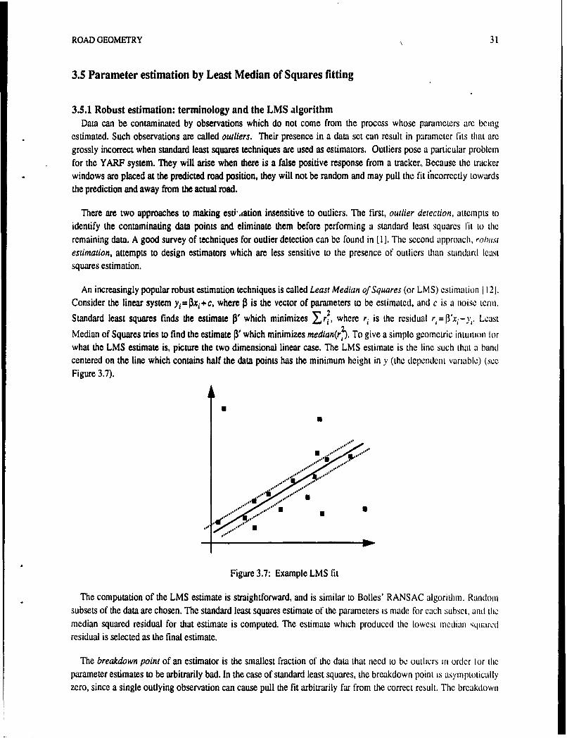
ROAD GEOMETRY 31
3.5 Parameter estimation by Least Median of Squares fitting
3.5.1 Robust estimation: terminology and the LMS algorithmData can be contaminated by observations which do not come from the process whose parameters arc being
estimated. Such observations are called outliers. Their presence in a data set can result in parameter fits that aregrossly incorrect when standard least squares techniques are used as estimators. Outliers pose a particular problemfor the YARF system. They will arise when there is a false positive response from a tracker, Because the trackerwindows are placed at the predicted road position, they will not be random and may pull the fit ihcorrectly towardsthe prediction and away from the actual road.
There are two approaches to making esti',ation insensitive to outliers. The first, outlier detection, attempts toidentify the contaminating data points and eliminate them before performing a standard least squares fit to theremaining data. A good survey of techniques for outlier detection can be found in [I]. The second approach, robustestimation, attempts to design estimators which are less sensitive to the presence of outliers than standard leastsquares estimation.
An increasingly popular robust estimation techniques is called Least Median of Squares (or LMS) cstimation 1I 21.Consider the linear system y1=I0xi+c, where 3 is the vector of parameters to be estimated, and c is a noise term.Standard least squares finds the estimate P3' which minimizes 7r?, where ri is the residual r,=P'x1-y,. Least
Median of Squares tries to find the estimate [' which minimizes median(r,'. To give a simple geometric intuition lorwhat the LMS estimate is, picture the two dimensional linear case. The LMS estimate is the line such that a bandcentered on the line which contains half the data points has the minimum height in y (the dependent variable) (seeFigure 3.7).
d
Figure 3.7: Example LMS fit
The computation of the LMS estimate is straightforward, and is similar to Bolles' RANSAC algorithm. Randomsubsets of the data are chosen. The standard least squares estimate of the parameters is made for each subset, and themedian squared residual for that estimate is computed. The estimate which produced the lowest median squaredresidual is selected as the final estimate.
The breakdown point of an estimator is the smallest fraction of the data that need to be outlicrs in order lor theparameter estimates to be arbitrarily bad. In the case of standard least squares, the breakdown point is asymptoticallyzero, since a single outlying observation can cause pull the fit arbitrarily far from the correct result. The breakdown

32 ANNUAL REPORT 1991
point of LMS estimation is 50%, the maximum achievable.
The relative efficiency of an estimator is the ratio of the lowest achievable variance for the estimated parameters(given by the Cramer-Rao bound) and the variance achieved by the given estimator. In the case of LMS estiationthe relative efficiency is 2/r=0.637. In practice, the variance in the parameter estimates can be reduced by usingthe value of the median squared residual to estimate the variance of the noise in the data, eliminating data pointsmore than three standard deviations away from the initial LMS fit, and refitting the remaining data points usingstandard least squares.
Two phenomena complicate the task of identifying outlying observations. The first, masking, occurs when thereare multiple ouliers in the data which jointly influence the fit in such a way that their residuals do not look unusual.,The second, swamping, occurs when outliers influence the fit in such a way that valid data points have suspiciouslylarge residuals which make them appear to be outliers. Selecting a robust estimation technique which shows lowsensitivity to masking is important in the YARF domain because outliers will occur near the predicted road location,and will therefore tend to influence the fit in a consistent way. LMS estimation shows little sensitivity to masking,another factor in its favor.
3.S.2 Examples showing the effects of contaminants on road shape estimationContaminating data points can arise from a number of sources. False positive responses from the low level image
segmentation techniques are the most obvious source, but changes in road appearance present another source.Figure 3.8 shows an example of this. In this experiment a human drove Navlab 11 on a local highway at a speed of45 miles per hour while YARF attempted to track the lane. Three successive fit results are shown from left to right.At the top of the first frame the right white stripe begins to curve off to the right for the exit ramp. The road isactually straight, but the fit curves off slightly. This error results in incorrect predictions for the feature locations inthe middle frame. The white stripe on the right is located as it veers off on the exit ramp, but the white str:)C on theleft has been lost (the asterisks represent the predicted feature locations where the tracker returned lailurc). In thethird frame on the right YARF is now tracking the exit lane while the vehicle continues in its lane, resulting in theleft edge of the reconstructed lane passing through the vehicle. While the data in this example is not dense enoughfor LMS to detect the error, it shows the way in which the contaminants can be highly structured.
The second example (Figure 3.9) shows a case in which the outliers are the result of errors in the segmentation.The lane being followed has a double yellow line on the left side and a single solid white line on the right side. Dueto error in the predicted road location some of the tracker. for the double yellow line are off the road on grass andreturn false feature locations. The road actually curves off to the right, explaining the tendency of the points from theleft lane edge to fall to the right of the fit in the middle of the diagram, and the failure of the white stripe tracker tolocate the right lane edge in that same area (the points marked with asterisks). The LMS fit on the right shows thecorrect road fit, with the erroneous feature points at top far off to the left of the lane.
3.6 ConclusionIn this chapter we have explained the motivation behind YARF's selection of road representation and model
fitting algorithms. We have shown how an analysis of the errors introduced by linearizing the circular arc roadmodel leads to the idea of performing virtual panning on the data to reduce the errors in the model paramcterestimates, and presented quantitative results from simulation runs to show the improvement from virtual panning.Also, we have explained the motivation for using least median squares estimation to avoid errors causcd by outlyingdata points
Future work would involve an attempt to characterize the errors induced in the parameter estimates in cases where
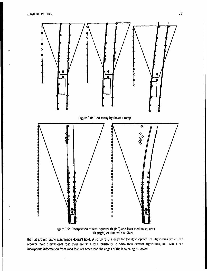
ROAD GEOMETRY 33
Figure 3.8: Led astray by the exit ramp
Figure 3.9:, Comparison of least squares fit (left) and least median squaresfit (right) of data with outliers
the flat ground plane assumption doesn't hold. Also there is a need for the development of algorithms which canrecover three dimensional road structure with less sensitivity to noise than current algorithmns, and which canincorporate information from road features other than the edges of the lane being followed.

34 ANNUAL REPORT 1991
References
[1] Beckman, R. J., and Cook, R. D.Outlier ......... s.Technometrics 25(2): 119-149, May, 1983.,
[2] Crisman, Jill.Color Vision for the Detection of Unstructured Roads and Intersections.PhD thesis, Carnegie-Mellon University, 1990.
[31 DeMenthon, Daniel, and Davis, Larry.Reconstruction of a Road by Local Image Matches and Global 3D Optimization.In Proceedings 1990 IEEE International Conference on Robotics and Automation., May, 1990.
[4] Kanatani, Kenichi, and Watanabe, Kazunari.Reconstruction of 3-D Road Geometry from Images for Autonomous Land Vehicles.IEEE Transactions on Robotics and Automation 6(1): 127-132, February, 1990.
[5] Kenue, Surender K.LANELOK: Detection of Lane boundaries and Vehicle Tracking Using Image-Processing Techniques -- Part
I: Hough-Transform, Region Tracing and Correlation Algorithms.In SPIE Mobile Robots IV. 1989.,
[6] Kenue, Surender K.LANELOK: Detection of Lane boundaries and Vehicle Tracking Using Image-Processing Techniques -. Part
II: Template Matching Algorithms.In SPIE Mobile Robots IV., 1989.
[7] Kuan, Darwin; Phipps, Gary; and Hsueh, A.-Chuan.Autonomous Land Vehicle Road Following.In Proceedings First International Conference on Computer Vision. June, 1987.
[8] Liou, Shih-Ping, and Jain, Ramesh.Road Following Using Vanishing Points.Computer Vision, Graphics, and Image Processing 39:116-130, 1987.
[9] Mysliwetz, Birger D., and Dickmanns, E. D.Distributed Scene Analysis for Autonomous Road Vehicle Guidance.In Proceedings SPIE Conference on Mobile Robots.. November, 1987,
[10] Polk, Amy, and Jain, Ramesh.A Parallel Architecture for Curvature-Based Road Scene Classification.In Roundtable Discussion on Vision-Based Vehicle Guidance '90 (in conjunction with IR OS). July, 1990.
[11] Pomerleau, Dean A.Neural Network Based Autonomous Navigation.Vision and Navigation; The Carnegie Mellon Navlab.In Charles E. Thorpe,Kluwer Academic Publishers, 1990, Chapter 5.
[121 Rousseeuw, Peter J. and Leroy, Annick M.Robust Regression and Outlier Detection.John Wiley & Sons, Inc., 1987.
[131 Schaaser, L. T., and Thomas, B. T.Finding Road Lane Boundaries for Vision Guided Vehicle Navigation.In Roundtable Discussion on Vision-Based Vehicle Guidance '90 (in conjunction with IROS). July, 1990.
[14] Turk, Matthew A., Morgenthaler, David G.; Gremban, Keith D.; and Marra, Martin.VITS -- A Vision System for Autonomous Land Vehicle Navigation.IEEE Transactions on Pattern Analysis and Machine Intelligence 10(3), May, 1988.

COMPUTATIONAL MODEL OF DRIVING 35
4. A Computational Model of Driving for Autonomous Vehicles
4.1 IntroductionDriving models are needed by many researchers.1 Intelligent vehicle designers need them to make driver aids that
work in dynamic traffic situations. Robot vehicle builders need them to drive vehicles autonomously in traffic.Traffic engineers need them to improve the safety of highways. To be most useful, a driving model must be detailedand complete. A detailed model must state specifically what decisions must be made, what information is needed,and how it will be used. Such models are called computational because they tell exactly what computations thedriving system must carry ouL A complete driving model must address all aspects of driving. In the course of ourresearch in robotics, we have developed a computational model that addresses a level of driving which has not beenpreviously addressed. We have implemented this model in a system called Ulysses.
The driving task has been characterized as having three levels: strategic, tactical and operational [27]., Theselevels are illustrated in Table 4.1. The highest level is the strategic level, which develops behavioral goals for the
Level Characteristic Example Existing model
Strategic Static; abstract Planning a route; Planning programsEstimating time for trip (Artificial Intelligence)
Tactical Dynamic; physical Determining Right of Way; Human drivingPassing another cai models
Operational Feadback control Tracking a lane; Robot control
Following a car systems
Table 4.1., Characteristics of three levels of driving.
vehicle. These goals may be based on route selection and driving time calculations, for example. The strategicgoals are achieved by activities at the middle, tactical, level, which involves choosing vehicle maneuvers within thedynamic world of traffic and traffic control devices (TCD's). The maneuvers selected at the tactical level are carriedout by the operational level of speed and steering control.
Substantial progress has been made in automating various parts of the driving task, particularly at the strategicand operational levels, but no system has yet implemented the tactical level. At the strategic level, planningprograms in the Artificial Intellig,'nce community are quite good at planning errands, finding routes, and performingother abstract tasks. However, they do not solve the problems of vehicle maneuver selection because they are notdesigned to work in a dynami. domain and without complete knowledge of the problem. At the operationl level.several robot projects have demonstrated the ability to drive a vehicle on roads that are essentially devoid ol trathIcand TCD's. These systems can track lanes, but have no real knowledge of driving laws and general \'chiclebehavior. Thus, they too avoid the problems of maneuver selection that form the tactical level of driving.
Traffic engineers and psychologists have long studied the driving task, including tactical driving, and have
'An earher version of thu report appeared as techmcam report CMU-CS-91-122, authored by Douglas Reece and Steven Shafer

36 ANNUAL REPORT 1991
developed many good theories and insights about how people drive. Unfortunately, these models of human drivingdo not explain exactly what and how information is processed-what features of the world must be observed, whatdriving knowledge is needed and how it should be encoded, and how knowledge is applied to produce actions. Amodel must answer these questions before it can be used to compute what actions a robot should take.
Our driving program, Ulysses, is a computational model of tactical driving. The program encodes knowledge ofspeed limits, headways, turn restrictions, and TCD's as constraints on acceleration and lane choice. The constraintsare derived from a general .desire to avoid collisions and a strategic driving goal of obeying traffic laws. Ulyssesevaluates the current traffic situation by deliberately looking for important traffic objects. The observations,combined with the driving knowledge and a strategic route plan, determine what accelerations and lane changes arepermitted in this situation. The program then selects the one action that allows the robot to go as fast as possible.While this model has limitations, it drives competently in many situations. Since it is a computational model,Ulysses shows exactly what information a driver needs at each moment as driving decisions are made. Furthermore,the program can be tested objectively on a real vehicle.
Our eventual goal is to use Ulysses to drive a real vehicle. At this time, however, the model has only beenimplemented in computer simulation. We have constructed a microscopic traffic simulator called PHAROS (forPublic Highway and ROad Simulator) [301 for our driving research. PHAROS represents the street environment indetail, including the shape and location of roads, intersections, lines, markings, signs, and signals. The cars inPHAROS are driven using a simplified version of the driving model. The simulator generates an animated displayof traffic that can be used to observe driving behavior. PHAROS performs the perception and control functions forUlysses so that Ulysses can drive a robot through a road network in simulation.
This chapter describes our driving model for robcts in detail. The next section reviews existing driving models,including both robot driving systems and human driving models. We then present Ulysses, and describe theimportant features of PHAROS. The chapter concludes with a discussion of possible extensions to the model andother future research.
4.2 Related Work
4.2.1 Robots and PlannersComputers have been used to automate several aspects of the driving task. Various research groups have been
investigating vehicle steering and speed control ,or it least 30 years [5, 13, 15, 24, 28, 34]. This work generallyassumes that special guides are placed in the roads, so the vehicles are not completely autonomous. In the 1980's,robots began driving on roads autonomously [9, 20, 22, 29, 36, 37, 38, 39,42]. The different robots have strengthsin different areas; some are fast (60 mph), while others are very reliable in difficult lighting or terrain conditions.Autonomous vehicles can also follow other vehicles, with or without a special guide device on the leadvehicle [4, 7, 14, 19, 21, 36].
These existing robot systems address only the operational level. Consider the driver approaching the intersectionin Figure 4.1 from the bottom. A robot with current operational capabilities could track the lane to the intersection,.find a path across the intersection, and then start following a new lane. The robot could also perhaps detect the caron the right and stop or swerve if a collision were imminent. However, in this situation a driver is required] tointerpret the intersection configuration and signs and decide whether it should pass in front of the other car. Currentrobot driving programs cannot perform this tactical task. Nevertheless, it is the success of automonous vchicles atthe operational level that motivates us to study the tactical level.,

COMPUTATIONAL MODEL OF DRIVING 37
... ...............
Figure 4.1: Example of tactical driving task: driver approaching crossroad.
Computers have also been used to automate strategic driving functions. Map-based navigation systems haveadvanced from research projects to commercial products in the last decade [3, 11, 18, 32, 35,411.. ArtificialIntelligence programs have been applied to many abstract problems, including the planning of driving errands 117 1.These planners work on static problems using information conveniently encoded in a database ahcad of time. Let u-Sconsider again the driver of Figure 4.1. A strategic planner may have already determined that this drivcr is going toa pizza store, and that he must turn left at this intersection, and that he should drive quickly because he is hungry.However, the planner (probably) does not know ahead of time what TCD's are present at this intersection, andccrtainly camot predict the arrival of cross traffic. Since the situation is unknown ahead of time, the driver must getdata by looking for signs and cars when he gets to the intersection. This data must be interpreted to form abstractconcepts such as "the other car is stopping." In general, the world is uncertain and dynamic at this level, and thedriver must continually use perception to assess the situation. Strategic planners are not designed to deal with thesetactical problems.
4.2.2 Human Driving ModelsPsychologists, traffic engineers and automotive engineers have studied human driving a great dal. Their goal is
to make cars and roads safer and more efficient for people. The result of this work is a multitude of driving modelsspanning all levels of driving. Michon identified seven types of models [27]:, task analysis, inforination flowcontrol, motivational, cognitive process, control, trait, and mechanistic.. Each has different characteristics andaddressed different aspects of driving.
Task analysis models. A task analysis model lists all of the tasks and subtasks involved in driving Theo pragiof these models is McKnight and Adam's analysis [26]. Their work provides an exhaustive breakdown ol allactivities on the tactical and orvrational levels. We have found this listing very useful for determining whether ourmodel performs all of the necessary su tasks in various situqtions. However, a list of tasks alone is not sufl icient hor
describing a driving model. This is because a task list does not address the dynamic relations between tasks The

38 ANNUAL REPORT 1991
list does not specify how the driver chooses a task in a given situation, or whether one task can interrupt another, orhow two tasks might be performed simultaneously (especially if they require conflicting actions). The McKnightwork also leaves situation interpretation vague. For example, two tasks require a driver to "observe pedestrians andplaying children" and "ignore activity on the sidewalk that has no impact on driving." However, there are nocomputational details about how to discriminate between these situations.
Informationflow control models. Information flow control models are computer simulations of driving behavior.Early computer models of drivers were essentially implementations of task analysis models [27]., As such, they havethe same weaknesses as the task analysis models. More recent microscopic traffic simulators such as SIMRO [6j,TEXAS [16], and NETSIM [12,43] do not have these weaknesses because they perform multiple taskssimultaneously. They also have the ability to start and stop tasks at any time in response to traffic. For example,NETSIM evaluates the traffic situation frequently (every second) and makes a fresh selection of appropriatesubtasks. NETSIM is not intended to be an accurate description of human cognitive processing, but it producesreawonable driver behavior in many situations. NETSIM is a direct ancestor of our system, PHAROS, which wedescribe later in this chapter.
NETSIM cannot be used as a complete driver model because it lacks several necessary components. There arcgaps in its behavior; for example, cars are discharged from intersection queues into downstream streets withouthaving to accelerate and drive normally to and through the intersecion. Neither does NETSIM contain knowledgeof how to interpra traffic conditions from observable objects. We also found unmodified NETSIM inadequate as asimulator testbed for robotics research because it cannot represent physical information such as road geometry,accurate vehicle location, or the 1oation and appearance of TCD's.
Motivational models. Motivational models are theories of human cognitive activity during driving. Van derMolen and Botticher recently reviewed several of these models [40]. The models generally describe mental statessuch as "intentions," "expectancy," "perceived risk," "target level of risk," "need to hurry" or "distractions." Thesestates are combined with perceptions in various ways to produce actions. Since motivational models attempt todescribe the general thought processes required for driving, one would hope that they would form a basis lor avehicle driving program. However, the models do not concretely show how to represent driving knowledge, how toperceive traffic situations, or how to process information to obtain actions. Van der Molen and Botticher attemptedto compare the operations of various models objectively on the same task [33, 40], but the mxlels could beimplemented only in the minds of the model designers. Some researchers are addressing this problem by describingcognitive process models of driving (for example, Aasman [1]). These models are specified in an appropriatesymbolic programming language such as Soar [23].
The remaining types of models have limited relevance to tactical driving. Control models attempt to desci ibe thedriver and vehicle as a feedback control system (e.g., [31]). These models are mainly useful for lane keeping andother operational tasks. Trait models show correlations between driver characteristics and driving actions. Forexample, drivers with faster reaction times may have a lower accident rate. This correlation does not describe themechanism by which the two factors are related. Finally, mechanistic models describe the behavior of traffic as anaggregate whole. These models express the movement of traffic on a road mathematically as a flow of fluid [10].This type of model cannot be used to specify the actions of individual drivers.
4.2.3 UlyssesIn this chapter we present a new computational model of driving called Ulysses. It is computational because it
explains how to compute driving actions from sensed data. Ulysses encodes knowledge for performing a variety oltactical driving tasks, including maneuvering in traffic on multilane highways and negotiating intcrsection.. Like

COMPUTATIONAL MODEL OF DRIVING 39
the information flow control models, Ulysses performs all appropriate tasks simultaneously., Ulysses goes beyondmodels such as NETSIM because it describes how to drive in the transitions between states (e.g. between free flowand enqueued). Unlike existing models, Ulysses makes decisions based on observable phenomena. The perceptualpart of driving is therefore described in terms of looking in specific areas for specific objects. This explicit situationassessment is much more concrete than the "risk perception" in the motivational models. Ulysses operationalizesconcepts such as "risk avoidance" in these models with specific constraints on lane selection and speed. SinceUlysses is implemented as a computer program (in the language Allegro CommonLisp), it can be analyzed andtested objectively. It can be used in various driving situations to study the perceptual and information processingrequirements of the task. And ultimately, Ulysses can be used to compute actions for an actual vehicle driving intraffic.
4.3 The Ulysses Driving ModelWe have implemented a computational driving model in a program called Ulysses. Ulysses defines a complete
system for driving - what a driver must look for, how situations are evaluated, what practical knowledge is needed,and how this knowledge is encoded and applied. Figure 4.2 is a schematic of the entire driver model. Only thetactical level is implemented in detail in Ulysses. The model treats the operational and strategic levels ilbstLoacflysince the details have already been addressed by other work. These levels are discussed tl the end ol the section.
Figure 4.2 shows that at the tactical level, Ulysses performs several perception and decision functions. Ulyssesuses the route plan created at the strategic level as a guide in scanning the road ahead along the intended route. Theportion of the strategic route plan that is actually visible to the robot is called the corridor in our model. Ulyssesidentifies the corridor at the tactical level so it knows which signs, signals and other cars are important. The corridoris built up incrementally as the Ulysses finds intersections and chooses which direction to look further. As thecorridor is found, implicit goals to drive lawfully and safely cause constraints to be generated. The constraints retriggered by the presence of various traffic objects. Ulysses must look for all objects that could trigger a constraint.After all constraints have been applied, Ulysses chooses an acceleration and lane-changing action from the availablechoices. This selection is based on the implicit goals of driving quickly and courteously. State variables are uscd torecord decisions such as accepting gaps in traffic that affect actions for a period of time. Table 4.2 sumniari/cs thestate variables used in Ulysses; these will be explained later in this section.
In order to be able to respond quickly to unpredictable events, Ulysses frequently repeats its visual search andevaluation of the current situation. The decision cycles have a period of lOOms. This rapid polling simulates theresponsiveness of perceptual interrupts. However, the polling scheme allows constraint evaluations to activateperception rather than the other way around. Ulysses uses this demand-driven perception at the tactical level toprovide a mechanism for focusing its perceptual attention. Focusing perception is important for robots becausemachine perception is very difficult; it would be impossible to perceive and analyze everything in the field of vicwin 100 ms.
In the remainder of this section we explain the specific driving knowledge in Ulysses by describing a scries olscenarios of increasing complexity. fhe scenarios include a simple highway with only one lane, intersections withvarious traffic control devices, and finally multi-lane roads. The section concludes with a discussion of perception,'strategic plans and operational control.

40 ANNUAL REPORT 1991
Perception Decision Action
Strategic
Tactical FindLook for intended
roadsroute ahead
Operati lCin
Figure 4.2: Schmaic of the Ulysses driver model
4.3.1. Tactical Driving Knowledge
4.3.1.1 A Two-Lane HighwayFigure 4.3 depicts a simple highway driving situation. In this scenario no lanechanging actions arc ncccssary,
but there are several constraints on speed.
The first two constraints are derived from general safety goals--i.e., self-preservation. The speed of thc v'chickcmust be low enough to allow it to come to a stop before the end of the road is reached; the speed on a curve mustkeep the vehicle's lateral acceleration below the limit imposed by friction between the tires and road surfce.

COMPUTATIONAL MODEL OF DRIVING 41
State Variable Values
Speed Limit <current speed limit>
In intersection Street, Intersection
Wait Normal, Wait for gap, Wait for merge gap, Accept
Lane Position Follow lane, Init-left (-right), Changing-left (-right)
Table 4.2: Ulysses state variables.
KEY:
Road Accelerationcurvature constraint:
Robot:
Figure 4.3:' The two-lane highway scenario.
Although it is possible that these constraints can be met by the operational level systems of the robot, thc prdicton
of future speed constraints from observations of distant conditions is in general a tactical activity. This is especially
true if future conditions are detected not by tracking road features but by reading warning signs. Ulysscs gnerate,,
the road end and road curvature constraints by examining the corridor. The robot must be stopped at the nd ol he
road if the road ends; furthermore, at each point of curvature change, the robot's speed must be less than that
allowed by the vehicle's lateral acceleration limit. Ulysses also scans along the right side of the corridor or igns
warning of road changes, and creates a speed constraint at the relevant signs.
These constraints-a maximum speed at a point somewhere ahead in the coridorarc typical ot the moon

42 ANNUAL REPORT 1991
constraints generated by various driving rules. Given the robot's current speed, we could compute a constantacceleration value that would yield the desired speed at the desired point. However, it is also possible to satisfy theconstraint by driving faster for a while and then braking hard. Figure 4.4 shows these two possibilities as curves Xand Y on a graph of speed versus distance. The figure shows that any speed profile is possible as long as it stays
Speeds
Time TO + one decision cycle period
.. Deceleration at maximum brakingrat a B(aB < 0):I " Z-- "............ ..........".',,,.
Robot start s =S C 2a B (0-d
state (DRSR ..
time T. X
Constraint:5c . "C Max. speed S c
at distance DC
DistanceDC d
KEY
X: Constant deceleration from initial state to constraint stateY: Constant speed, then deceleration at maximum braking rateZ:' Acceleration for one decision cycle period, then maximum braking
Figure 4.4: Deceleration options plotted on speed-distance graph
below the maximum brakin, curve. The profile that maximized vehicle speed would rise instantly to the maximumbraking curve and then follow the curve to the constraint point. However, the program cannot change theacceleration command at arbitrary times; it looks at situations and changes acceleration only at discrete intervals.Therefore Ulysses computes an acceleration that will cause the robot's speed to meet the maximum decelerationcurve exactly at the next decision time. This is curve Z in the figure.
While the high-acceleration, high-decelerati ilicy shown by curve Z maximizes vehicle speed, it seems tohave the potential to cause jerky motion. In f&, ..x motion is usually smooth because the constraints relax as thcrobot moves forward. For example, suppose that the robot's sensors could only detect the road 150 fect ahcad.Ulysses would constrain the robot to a speed of 0 at a distance of 150 feet. However, when the robot movedforward, more road could be detected, so the constraint point would move ahead. Figure 4.5 shows how this "rollinghorizon" affects speed. The robot starts at distance 0 with a speed of 45 fps. A decision interval of 1.0 seconds isassumed in order to show speed changes more clearly.. The dashed lines show deceleration constraint curves (-15fps2) at the first four decision times. The solid line shows the robot's speed. After a small overshoot, the speed

COMPUTATIONAL MODEL OF DRIVING 43
80 , 1,%
70 %5* \
60 "%
50 \ ,
Speed, 40 -fps \ \
30 -\ \
20 -I ,\ '
10 -
0III I I
0 100 200 300 400 500 600Position, feet
Figure 4.5:, Robot speed profile (solid line) as it adjusts to a rolling road horizon.Maximum deceleration is -15.0 fps2, decision time interval 1.0 see, horizon at 150 feet.The four dashed lines show, for the first four decision times, the maximum-decelcration
profile to the current horizon.
reaches an equilibrium and remains constant.
The next constraint illustrated by Figure 4.3 is that generated by legal speed limits. Ulysses mainains a siatt'variable which records the current speed limit. The vehicle is allowed to accelerate so that it reaches the sI)eCdl Iiiiitin one decision cycle period. Furthermore, Ulysses scans the right side of the corridor for "Speed Limit" signs.Whenever the system detects a speed limit change, it creates an acceleration constraint to bring the robot's spced tothe limit speed at the sign (as described above). As the robot nears the Speed Limit sign, Ulysses also updates thespeed limit state variable.
The final acceleration constraint is generated by traffic in front of the robot. The safety goal implicit to Ulyssesrequires that an adequate headway be maintained to the car in front of the robot in the same lane. Ulysses thereforescans the corridor to monitor the next car ahead. If the lead car were to suddenly brake, it would come to a stopsome distance ahead. This is the constraint point for computing an acceleration limit. The program uses the leadcar's speed, its distance, and its assumed maximum deceleration rate to determine where it would stop. This activityis commonly called "car following."
After all acceleratio! constraints have been generated, they are combined by taking their logical intersecton. Theintersection operation guarantees that all constraints are met simultaneously. Figure 4.6 illustrates thi s process.Since the constraints in effect allow a range of accelerations between the negative limit (the braking capability ol therobot) and a computed positive value, the intersection results in a range from the negative limit to the smallestcomputed positive value. Ulysses chooses the largest allowed acceleration in order to further the implicit goal of

44 ANNUAL REPORT 1991
R e nd.. .
Range ofaccelerations . ......... Curvatureallowed by
various constraints(examples) Car following
Sedlimit
Logical intersection Rslof cosritsRsl cclrto
Maximum 0 Maximum accelerationbraking at current speed
Figure 4.6: Combining acceleration constraints.
getting to the destination as quickly as possible.
The perception system may not be able to detect objects beyond some range. Ulysses deals with the resultinguncertainty by making two assumptions: first, that there is a known range within which perception is certain; andsecond, that objects and conditions that trigger constraints are always present just beyond this rangc. This latterassumption is the worst case. For example, Ulysses always assumes that the road ends just beyond road-detectionrange, that the speed limit drops to zero just outside of sign-detection range, and that there is a stopped vehicle justbeyond car-detection range. In this way Ulysses prev.,nts the robot from "over-driving" its sensors.
4.3.1.2 An Intersection Without TralficThe next traffic scenario we consider is a simple inters'iction with only one lane on thc robot's approach, no other
traffic, and no pedestrians. Figure 4.7 illustrates this scenxio. Ulysses detects intersections when It visually tracksa lane ahead and finds that the markings end or the road braoches. Other clues, such as traffic signals or signs (orcars, in a different scenario), may be detectable at longer ranges; however, since the robot is constrained to stopanyway at the end of the detected road, Ulysses does not consider these clues. Future versions of Ulysses maymodel the uncertainties of machine perception in more detail and use several clues to confirm observations.
When the robot is actually in an intersection, Ulysses can no longer detect a lane directly in front o1' thc robot.When this first happens, Ulysses changes the In Intersection state variable from Street to Intersection. Later, whenthere is a lane in front of the robot, the state is changed back again. These state changes mark the robot's progrress inits strategic route plan.
Finding the corridor is more difficult at an intersection than it is on a simple highway becaUSC the corridor nolonger follows clearly marked lanes. The perception system must recognize the other roads at the intersection andlidentify the one on which the robot's route leaves. Figure 4.8 shows that the perception system must identify the"left" road if the strategic route plan requires the robot to turn left at this intersection. Ulysses can then extend the

COMPUTATIONAL MODEL OF DRIVING 45
,. .. ~ '. '. . . ..... . .. .. .. . .
Figure 4.7: An intersection without traffic; detection by tracking lanes.
corridor by creating a path through the intersection from Lhe end of the robot's approach road to the stirt ol theproper lane in the road on the left.
With the corridor established through the intersection, Ulysses generates the same acceleration constraints as borLhe highway case. Figure 4.9 shows several examples of how these constraints may apply at an intersection.Constraints may apply to conditions before, within, and beyond the intersection.
The next task for the driving program is to determine the traffic control at the intersection. In this scenario theonly important TCD's are traffic signals, Stop signs and Stop markings. Thus, as shown in Figurc 4.10, Ulysiesrequests the perception system to look for signs and markings just before intersection and signal heads at %ariousplaces around the intersection. When the intersection is beyond the given detection range for these objects, Ulyssesassumes the worst and constrains the robot to stop at the intersection; however, within the detection range Ulyssesassumes that all existing traffic control devices will be found.
Figure 4.11 diagrams the decision process for traffic signals required at this simple intersection. First, Ulyssesmust determine what the signal indication is. If there is an arrow in the direction of the corridor, the programn takesthis as the effective signal; otherwise, the illuminated solid signal is used. If the signal indication is red,, Ulyssesgenerates an acceleration constraint that stops the robot at the entrance to the intersection. No constraint INgenerated if the signal is green. If the signal is yellow, then Ulysses determinies whether the robot can be stoppe)d atthe intersection using a reasonable braking rate. If so, then the program generates a Constraint as i[ the light werered.

46 ANNUAL REPORT 1991
Lef t .
.vw4;.' KEY,-,
~ ~ . . *. Robot identification ofapproach road:
Corridor:
Figure 4.8: Finding the corridor for a left turn.
..Loa nd .J.I.E h
4 KEY:
*1 Acceleration'.: ~constraint:
Roa
Figure 4.9., Examples of acceleration constraints from road features atan intersection.
Stop signs require not only speed constraints, but a short sequence of actions. A vehicle approaching a stop sign

COMPUTATIONAL MODEL OF DRIVING 47
S....... . ...
;,',A ...... ..,..,t '1 .. . '
.~~~ .. , ' , .. . .. ,
Figure 4.10: Looking for possible traffic control devices at an intersection.
Stop robot atintersection
Signal color is the I 1color of arrow Yes
"oCan robot stopa rridor ? | before
Signal color isintersetin?
the solid color No
Noconstraints
Figure 4.11: Traffic signal logic for intersection without traffic.
must come to a complete stop, look for traffic, and then proceed when the way is clear., Figure 4.12 shows howUlysses performs these actions with a "Wait" state variable. When a stop sign is detected, Ulysses gcilerates aconstraint to stop the robot just before the sign. Later, Ulysses finds that the robot is stopped and that it i; \,cry nearthe sign, so it changes to a "wait for gap" state. In this scenario there is no traffic, so Ulysses immediately moves onto tie "accept" state and releases the robot from this traffic control constraint.

48 ANNUAL REPORT 1991
Normal , Wait for gaP- Robot is stopped
-Detect Stop sign * Robot is at Stop sign(Immediate;
no traffic)Stop robot at sign I -
Accept_____ _ •Robot crosses
intersection
KEY: Condition: • Robot is stopped
State: Accept
Figure 4.12: State transitions in Stop sign logic.
4.3.1.3 An Intersection with TraMc
We will now add traffic to the simple intersection scenario. Ulysses considers three kinds of traffic atintersections: cars in the same corridor as the robot, which must be given headway; cross traffic blocking theintersection; and cars approaching the intersection on other roads which may have to be given the RoW. Humandrivers are sometimes taught to watch the traffic behind them, in case another car is following too closely orapproaching very fast. In such a case the driver could accept lower gaps or make more aggressive judgements at inintersection, thereby continuing through the intersection and not stopping quickly in front of the following car.Ulysses does not make such judgements, and thus does not look for traffic behind the robot.
Figure 4.13 illustrates the first kind of traffic that Ulysses considers. The driving program must generatecar-following constraints from a lead car either in or beyond the intersection. If the lead car is turning oil' therobot's path, the robot must still maintain a safe headway until that car is clear of the path., Similarly, the robot mustmaintain a safe distance to cars that merge into its path.
The second kind of traffic that Ulysses looks for is cross traffic in the intersection., This includes cars sittng
across the robot's path or about to cross it, as shown in Figure 4.14. Since the law requires that a vehicle yield theRoW to vehicles already in the intersection, Ulysses looks for such vehicles and stops the robot belore theintersection if it finds one. Ulysses does not currently search beyond the closest car to find a gap. Future extensions
to Ulysses may try to time the robot's arrival at an intersection to the presence of an upstream gap. However, thistype of behavior could only be allowed if it were safe-that is, if the robot could still stop at the intersection itf tratlic
changed unexpectedly.
The third type of traffic is traffic approaching the intersection on other roads. The driving program analy/cs
nearby TCD's and this approaching traffic to determine if the robot has the RoW. After RoW is determined,Ulysses may generate an acceleration constraint and change the Wait state of the robot. Figure 4.15 illustrates thisprocess.

COMPUTATIONAL MODEL OF DRIVING 49
intersection M n
Figure 4.13: Potential car following conditions at an intersection.
Figure 4.14: Cars blocking an intersection.
Traffic Control Devices. First, Ulysses detects and analyzes signs, markings and traffic lights. In add.tion to thcTCD's needed for the previous scenario, the program now must recognize Yield signs and dcterinin, how iaiilanes are in the roads. The lane count is used to determine if the robot is on a "Minor Road-that is, il the robot s

50 ANNUAL REPORT 1991
r o Devices ae State-LightsSigns•Signals i
DetermineRight of Way
Approaching- Generate
,Traffic Constraint
Figure 4.15: Generation of constraints from traffic and traffic control.,
road has only one or two lanes and the other road has mor lanes. In the United States traffic on a Minor Road
generally yields the RoW to other traffic, so in effect has a yield sign. This is a practical rule, not a legal one.
Table 4.3 summarizes the meanings of the various TCD's. The figure groups the TCD's into four equivalcnceclasses. Yellow signals are treated as either red or green, depending on the robot's state and speed. If the robot is ina "wait for gap" state, a yellow signal is always treated as green. This practical rule allows the robot to pro, ecdthrough an intersection just before the signal turns red. This allowance prevents the robot from being stuck foreverin heavy traffic with no gaps. Cars with a given TCD normally yield the RoW to traffic with a TCD in a higherpriority class, as will be explained below. Note that some actions in the figure do not depend on other cars- forexample, red lights always stop the robot.
Approaching traffic., The second part of RoW evaluation is analyzing the robot's situation relative to other cars.This situation depends on the position and speed of the robot and other cars, and the relative position of the approachroads. Figure 4.16 shows how this information is combined with traffic control information to decide the RoW withrespect to each car., For each approach, Ulysses looks up the road to find the first car in each lane. The road to theright is ignored if the robot is turning right, as is the directly opposing road unless the robot or approaching car areturning left. Looking "up the road" essentially requires the perception system to find a corridor along a differentroad. If the perception system does not find a car, Ulysses makes RoW decisions as if there were a car at the rangelimit of the sensors or of sight distance. This hypothetical car is assumed to be going a little faster than theprevailing speed of traffic. If the approaching car is going too fast to stop before the intersection (assumng anominal braking rate), Ulysses always yields the RoW. On the other hand, if the car is very far away from theintersection. lJlyv.qe will ignore ir "Very far away" means that the time it will take the robot to cross theintersection at its current acceleration rate is less than the time it will take for the other car to reach the intersection.
If none of the above conditions exist, then Ulysses further analyzes RoW based on traffic' control devices and themovements of the other cars. First, Ulysses guesses the traffic control for the approaching car. To do this, theperception system must look at the side of the approach road for a sign (the back side of a sign). If there is no sign,,and the robot is facing a traffic light, Ulysses assumes that the approaching car also has a traffic light. If the car is

COMPUTATIONAL MODEL OF DRIVING 51
Traffic Control Action" Increasing priority
Green signal Use RoW rules
OR Nothing (see Figure 3-15)
Yield sign, Yield to traffic with Green or ";Yl sno traffic control;OR otherwise use RoW rules
Nothing and on Minor Rd (see Figure 3-15).,
Stop sign, Stop at intersection;OR then proceed using
turning right at Red RoW rules (seesignal when allowed. Figure 3-15)
Red signal Stop at intersection
IF Wait-state is "normal"ANDrobot can stop at intersection
Yellow signal THEN
treat as Red signalELSE
treat as Green signal.
Table 4.3: Actions required by four classes of Traffic Control Device
approaching from a cross street, the light is assumed to be red (when the robot's is green), and otherwise green.2
Once the program has an estimate of the approach car's traffic control, it compares the control to that facing therobot. If they are not equivalent, then the vehicle with the lowest priority signal is expected to yield the RoW.
If the traffic control for the approaching car and the robot are equivalent, Ulysses performs further analysis of thesituation. If the approaching car is close to the intersection and stopped, the program assumes that it is waiting for ,gap in traffic. In the case of a Stop sign, the robot takes the RoW if the approaching car is not yet waiting.Otherwise, if one or both vehicles are moving, then the robot yields the RoW to cars on the right, and to cars aheadwhen the robot is turning left. If both the robot and the approaching car are stopped and waiting for a gap, then thedrivers must use some deadlock resolution scheme to decide who goes first. In human drivers we have identifiedfour such schemes, as illustrated in Figure 4.17. Humans use different schemes, depending on the local custom andthe driver. Ulysses bases its decision only on road configuration; it will use the first-arrive,, first-leave technique :iswell when we better understand how to recognize the same cars in images taken at different times.
After determining the requirements of the traffic control devices and evaluating the traffic situation, Ulysses may
2rhis is a particularly clear example of how .ae explicit, computauonal rules in Ulysses elucidate the infonnation requiremenLS ot dr1% 1118.Drivers must make assumptions about the TCD's controlhng other cars, and sometimes make errors if their assumptions are wrong

52 ANNUAL REPORT 1991
Car in conflict? No Robot can proceed
lYes
Car can stop? Robot yields RoW
Yes
Robot and approaching No Base RoW oncar have same trafficproiyfsgnlcontrol? priority of signals
Yes
Stop sign and has not * Robot takes RoWyet stoppedl? 7-
Robot and car are Yes Resolve RoW deadlock .both waitng for a gap? (see Figure 3-16) ]
N oBase RoW on_
road configuration 7 FFigure 4.16: Right of Way decision process.
'R' is the robot, 'C' is the other car.
create an acceleration constraint and update the wait state. Figure 4.18 shows the conditions for changing states andfor constraining the robot to stop at the intersection. Note that once the program has decided to accept a glap andtake RoW, only the presence of new cars in the robot's path will cause it to stop again.

COMPUTATIONAL MODEL OF DRIVING 53
.... .. ....' ....t
2 : . LZZ, ?,
Yield to car on right Left turn yields toopposing traffic ......
b. Order of arrival. (t# is thea. Road Configuration time of arrival)
B
A
AC
t2
c. Opportunity. Car A is blocked by car d. Driver aggressiveness. Driver in carB, so car C can proceed. A is most aggressive.
Figure 4.17:. Right of Way deadlock resolution schcmes.

54 ANNUAL REPORT 1991
Normal WifogaN Robot is stopped AND 10 Wait for gap
Stop robot at (- Robot Is at Stop sign OR Stop robot atintersection IF -Signals allow robot to proceed) intersection IFsignals require signals requireor robot must or robot mustyield yield
Robot crosses Stop robot for ' Signals allow robot to proceedintersection cross traffic AND
- Robot has RoW
KEY Condition: * Robot is stopped
State: Accept i
Figure 4.18: Changes in the Wait state at an intersection.
4.3.1.4 A Multi-lane Intersection ApproachThe driving situations considered so far have not included streets with multiple lanes. With this complication,
Ulysses must generate lane use constraints and make lane selections. We first consider the simple case of multiplelanes at an intersection, as depicted in Figure 4.19. In this scenario there is no other traffic on the same road as therobot.
As the robot approaches an intersection, constraints on turn maneuvers from different lanes-which we generallyrefer to as lane channelization- determine the lane-changing actions that Ulysses can take. Ulysses determines ifthe channelization of the robot's current lane is appropriate, and looks for a better lane if it is not. Channeization isestimated first by finding the position of the current lane at the intersection. If it is the left-most lane, then theprogram assumes that a left turn is allowed from the lane; similarly with right turns if it is the right-most lane.Through maneuvers are allowed from any lane by default. Ulysses also looks for signs and road markings to modif-yits assumptions about channelization.
If the robot's intended maneuver at the intersection is not allowed by the channelization of the robot's currentlane, Ulysses generates an acceleration constraint to stop the robot before the intersection. Figure 4.20a illustratesthis constraint. Ulysses estimates the minimum distance rquired to change lanes (from the width of the lanes andthe robot's minimum turn radius) and stops the robot that far from the intersection. The program next decides inwhich direction the robot should move to correct the situation, and looks to see if there is a lane on that side of therobot. If there is a lane, Ulysses constrains the robot to take a lane-change action in that direction. As a practicalmatter, solid lane lines are ignored, because making a turn from the correct iane is more important than strictl,obeying these lane-change restrictions. Since there is only one allowed action, no selection preferences need Ieconsidered.
Once a lane-changing action is started, Ulysses makes sure that the robot completes the maneuver before it enters
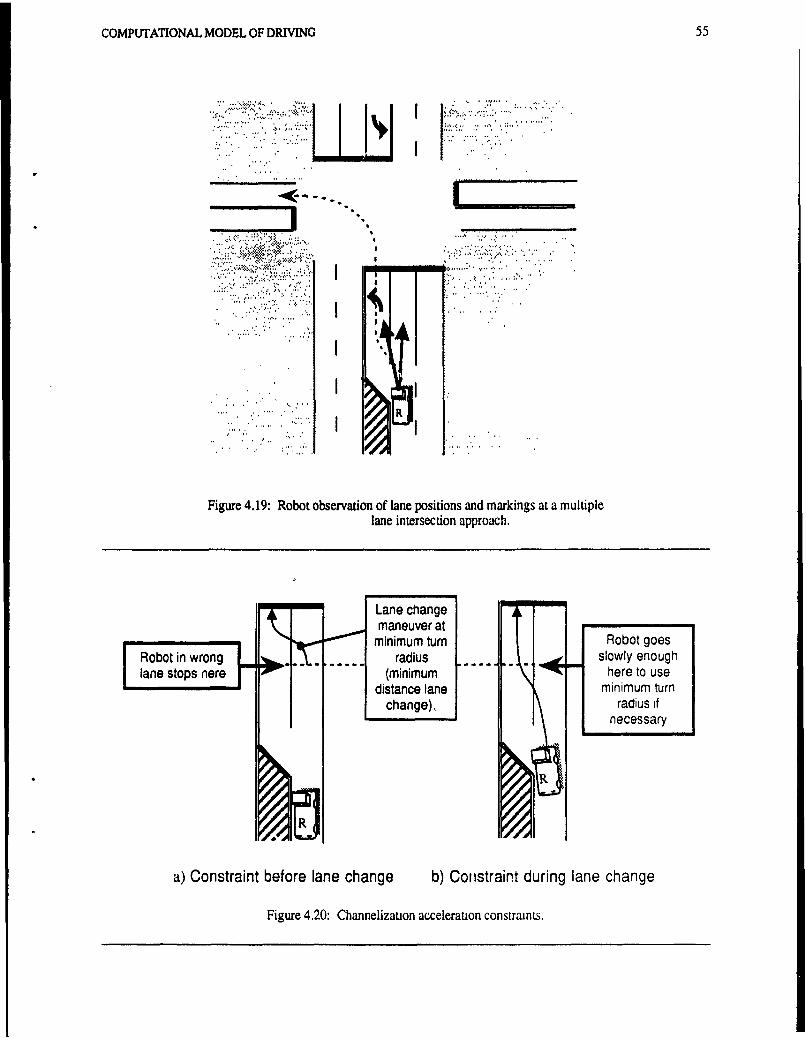
COMPUTATIONAL MODEL OF DRIVING 55
. . . : .. '... .. ...... .
. . ... .. _.
R
Figure 4.19: Robot observation of lane positions and markings at a multiplelane intersection approach.
minium urnRobot goesRobot in wrong ... slowly enough
lanestop ner (miimumhere to usedistance lane minimum turn
change), radius fnecessary
a) Constraint before lane change b) Constraint during lane change
Figure 4.20: Channelization acceleration constraints.
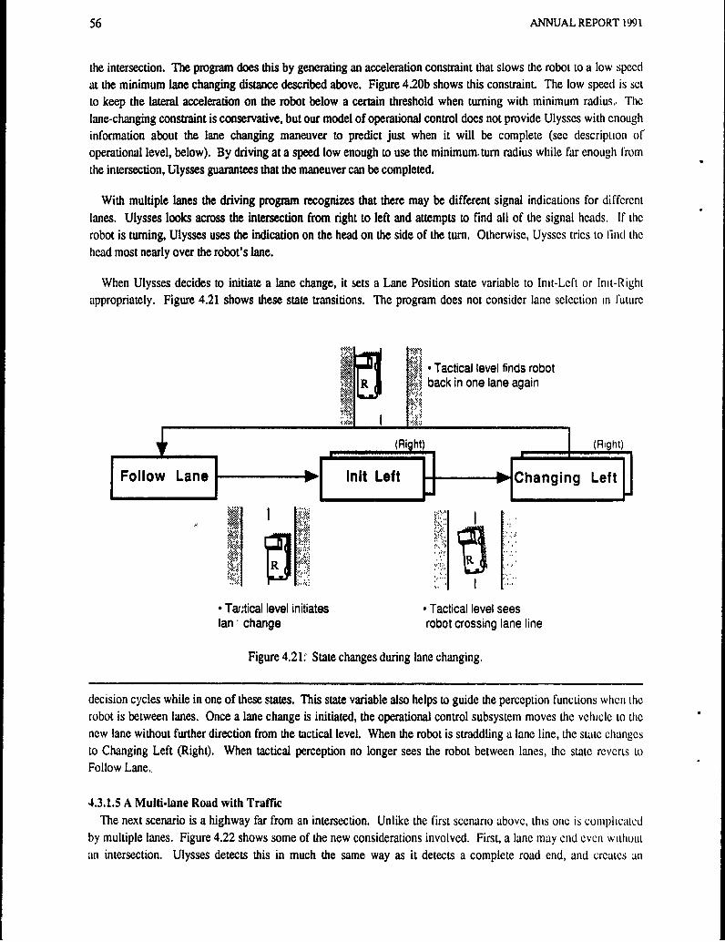
56 ANNUAL REPORT 1991
the intersection. The program does this by generating an acceleration constraint that slows the robot to a low speedat the minimum lane changing distance described above. Figure 4.20b shows this constraint. The low speed is setto keep the lateral acceleration on the robot below a certain threshold when turning with minimum radius. Thelane-changing constraint is conservative, but our model of operational control does not provide Ulysses with enoughinformation about the lane changing maneuver to predict just when it will be complete (see description ofoperational level, below). By driving at a speed low enough to use the minimum, turn radius while far enough fromthe intersection, Ulysses guarantees that the maneuver can be completed.
With multiple lanes the driving program recognizes that there may be different signal indications for differentlanes. Ulysses looks across the intersection from right to left and attempts to find all of the signal heads. If therobot is turning, Ulysses uses the indication on the head on the side of the turn. Otherwise, Uysscs tries to find thehead most nearly over the robot's lane.
When Ulysses decides to initiate a lane change, it sets a Lane Position state variable to Imit-Left or Init-Rightappropriately. Figure 4.21 shows these state transitions. The program does not consider lane selection in future
Tactical level finds robotR back in one lane again
X
Ta tical level initiates • Tactical level seesIan, change robot crossing lane line
Figure 4.21. State changes during lane changing.
decision cycles while in one of these states. This state variable also helps to guide the perception functions when therobot is between lanes. Once a lane change is initiated, the operational control subsystem moves the vehicle to thenew lane without further direction from the tactical level. When the robot is straddling a lane line, the state changesto Changing Left (Right). When tactical perception no longer sees the robot between lanes, the state reverts toFollow Lane.,
4.3.1.5 A Multi.lane Road with TraffcThe next scenario is a highway far from an intersection. Unlike the first scenario above, this one is complicated
by multiple lanes. Figure 4.22 shows some of the new considerations involved. First, a lane may end evcn withoutan intersection. Ulysses detects this in much the same way as it detects a complete road end, and creates an

COMPUTATIONAL MODEL OF DRIVING 57
Next car ahead,if lead car is Weichanging lanes - ' = ! a ee c
Ledcri e Leadl car in oldlan lane
11, I,:,.'"
,"Figure 4.22: Multiple lane highway scenario.
acceleration constraint to stop the robot before the end of the lane. This constraint disappears after the robotchanges lanes. Multiple lanes also make car following more complex. If the car in front of the robot is between twolanes, Ulysses maintains a safe headway to that car but also looks for another car in the lane. If the robot is itselfchanging lanes, the program looks ahead for cars in both lanes until the robot has cleared the old lane.
The three lane actions available to the robot are following the current lane, moving to the right, or or moving tothe left. Moving to the left does not currently include moving into the opposing lanes; thus Ulysses cannot yetovertake when there is only a single lane in each direction. Ulysses generates contraints and preferences forchanging lanes if certain traffic conditions exist. Figure 4.23 shows the important cona *ions: adjacent lanes, gapsin traffic in adjacent lanes, blocking traffic in the robot's lane and blocking traffic in adjacent lanes. In this scenario,,the program does not need to consider channelization.
Table 4.4 shows the constraints and preferences for each traffic condition. The absence of adjacent lanes orbroken lane lines or gaps in traffic eliminates the option to move to adjacent lanes., Ulysses generally prel'ers therightmost lane to others. Traffic blocks the robot if the acceleration allowed by car following is signiticantly lessthan acceleration allowed by other constraints. Blocking traffic creates a preference for an adjacent lane it theacceleration constraint in that lane is significantly higher than the car following constraint in the current lane.Ulysses estimates the allowed acceleration in the adjacent lane by hypothesizing what the car following constraintwould be and combining this with the speed limit, lateral acceleration and road end constraints. The programcombines the constraints from various conditions by taking their logical intersection-retaining only actions thatappear in all constraints. If there is more than one lane action available after constraints have been combined,preferences determine which action is chosen. Preferences due to blocking traffic are given priority over therightmost lane preference.
Ulysses judges gaps for changing lanes based on two criteria: first, the deceleration required of the robot to cICatca safe headway to the lead car in the other lane; and second, the deceleration required of the following car to leave'space for the robot. The program does not search for a gap farther back in traffic if the adjacent one is not big

58 ANNUAL REPORT 1991
Blocker
Presence of otherlanes
Position of robot'slane
•Lane lines
Figure 4.23: Traffic objects that affect lane changing decisions.
enough. However, if the robot is blocked, traffic in the adjacent lane will tend to pass the robot, thereby providingnew merging opportunities. Ulysses also does not have the ability to use a physical "language" (beyond directionalsignals) to communicate to other drivers that it is anxious to change lanes. It is thus possible that the robot willnever find a gap if traffic is congested.
4.3.1.6 Traffic on Multi-lane Intersection ApproachThe next scenario combines the previous two multi-lane cases. This situation, illustrated in Figure 4.24, adds
channelization constraints to traffic considerations. When the adjacent lane does not permit the robot's next turn,Ulysses must decide whether a pass can or should be made. Similarly, if the robot needs to move to a turn lane thathas traffic in it, Ulysses must decide whether to merge immediately or wait. Table 4.5 lists the constraints andpreferences that must be added to those in Tabsi 4.4. When combining preferences, Ulysses gives thechannelization demands the highest priority unless the robot is far from the intersection.
When the robot is near the intersection (d DF< r in Table 4.5), it is not allowed to change lanes to move awayfrom an acceptable ("OK") lane. Thus Ulysses will not attempt to pass a blocking car near an intersection unlessmultiple lanes are acceptable. This restriction may cause the robot to get stuck behind a parked vehicle, but it avoidsthe problem of deciding whether the lead vehicle is really blocking the road or just joining a queue that extends allthe way to the intersection.
The "Far from intersection" (d > Dar) condition in Table 4.5 depends on a distance threshold D r . When theintersection is at least DFar away from the robot, Ulysses can pass blockers rather than staying in a turn lane. Thethreshold distance is properly a function of traffic-how far traffi- is backing up from the intersection, whether thereare gaps in the traffic ahead of the blocker, and how iong (distance) the robot would take to complete a pass.Ulysses determines DFar by estimating passing distance and adding a margin to cover the other conditions. Themargin is a function of the speed limit, but does not explicitly incorporate downstream queuing condition,. In oursimulated world we have found that the margin needed to minimize inappropriate passing maneuvers puts thef robot

COMPUTATIONAL MODEL OF DRIVING 59
SET OFCONDITION ALLOWED PREFERRED Increasing
ACTIONS ACTION Priority
Blocking car • L- C > T1 AM LAll Move LeftA
(Robot Broken lane lineblocked by *R-C>Ttraffic in 1 All Move Rightlane*) Brc ,en lane line
-C > R, L All Keep Same
Gap for
merging
-No gap in traffic to left (Move Right, Keep Same)-No gap in traffic to right (Move Left, Keep Same) -
Availablelanes
'There is no lane to the left (Move Right, Keep Same) -
-There is no lane to the right (Move Left, Keep Same) -
-(There is a lane to the right) All Move RightAND (R C)
Default All Keep Same
KEY * True when (Car following accel) <(Other accel constraints) -T2Ti: Arbitrary threshold value.
L, P, C: Max. acceleration allowed in the lane to the Left, laneto the Right, and Current lane, respectively
Table 4.4: Lane action preferences for a highway with traffic.,
in the "near intersection" condition soon after it detects the intersection.
The presence of traffic introduces additional factors into the tests of blocking conditions. When Ulyscsdetermines what acceleration is possible for the robot in an adjacent lane, it must consider constraint. from lanechannelization and intersection traffic control. In effect, Ulysses must hypothesize the robot in the adjacent lane,look ahead in a new corridor, and recompute all of the acceleration constraints from that lane.
When the robot wishes to change lanes because of channelization, but cannot because that lane change action isnot allowed (for example, because a gap in traffic is not available), Ulysses changes the robot's Wait state to "wait

60 ANNUAL REPORT 1991
Fig i i"u "a"i'
robot. ~ Figure 4.245 Ddeiioisats multiple ae intersectionsaedothrbt app roch stretTh e drfi vignoleg
alred erbed ."Tis sufcientsgasasaigdsr to ghngeats We the robot thrug suc atiutinhis scnroilstatethh,yses
adjtesction aluton o the crodloowing througraintrsto n ona cxrsse istrets frntpoahrotfranuring.crs
4.3,. Tcticl sPercepnetion sThecfial comingdciions eqie inmtionaouleas intersections clnes, pasthough toetertesections alaneh
liroad mingu s.5eigns, minl, andters.Oiving ode asuesta the robot has oa crspsreepriinknowledgentateay detcttes trafficioets an determine throcationc an voctuainatin this penr ilsrteptionughs,.tmustesite he traitnce to orrojaects theg distnce beteersects, andzn theaffoity aof traffi Tontroe is% merpneretion aon the oriol and trateing lvbtrog wnersdono drss te ts modeppoahngcas
Tactical driv ,ingdeion require information about oadsaintersetions , bewen nbes. W h les throug fotretinsJ, atlins rall rinteste injcs thgas have aseii Orelaiving tod anomshtther ojc.fgro.oiuthats th cncept. Iyt nthat figureeUlysses itafint objects analyserine wheitri loai~io cars veonthe rnaigthand ,he prodtion sysi,
second intersection ahead. There are at least two ways to find the objects in the desir0~ relations. One way wouldbe to detect all cars, and then test each car to see if it was on the road to the right at the intersec:. on. "Thc road ",)the right" would itself be found by finding all roads and checking to see if they connected to tne the r,)txc i's roa(', atthe intersection in question. This method would be very difficult because thicie may be many cars anml roads vi th4robot's field of view, and each one requires significant computation to l'ind and test.

COMPUTATIONAL MODEL OF DRIVING 61
SET OFCONDITION ALLOWED PREFERRED PRIORITY
ACTIONS ACTION
Channelization
d < DMin Keep Same Highest
Current (Keep Same,lane OK Move to <OK lane>) -• DMidD -~aCurrent (Keep Same,lane not OK Move to <OK lane>) Move to <OK Lane>
Just belowd>D All Move to <OK Lane> Blocking Car
Far in Table 3-3
* No intersection visible All
KEY d: Distance from robot to intersection
oMn: Minimum distance needed to change lanes.
" Range of influence of intersection on upstream traffic
OK: Channlizaftion allows robot's intnded route
Table 4.5: Lane action constraints and preferences at an intersectionwith traffic.
Ulysses uses a different technique to relate objects to one another. The perception subsystem uses the rclcrecicobject and a relation to focus its search for a new object. In the example above the robot would track the corridorahead to the second intersection, scan to the right to find the approach road, and then look along the road for a car.The car detection process is thus limited to a specific portion of the field of view, determined by the location of theroad. All objects found are identified implcitly by their current relation to the robot. (This object identificationmethod has been called "indexical registration" by Agre and Chapman [2].) Ulysses gathers almost all of its datausing these perceptual routines. Table 4.6 lists the perceptual routines used by the program. Although it may seemthat driving decisions could be made with simpler, more general sensing functions, Figure 4.26 shows that verysimple sensing is not sufficient; "detect converging objects to the right," for example, cannot distinguish between thetwo intersections.
The perception subsystem uses markers to provide reference points for the perceptual routines. Our simple modelof se.nsing currently assumes that one image-a snapshot picture of the world-is taken each time Ulysses rcpeat',its decisions. Markers are placed in an image as a result of running perceptual routines that can mark cars, laneendings or beginnings, signs, markings, signal heads, or other locations. The markers are essentially names thatdifferent perceptual requests can use for the objects in an image. In the example of Figure 4.26, varioas routineswould put markers in the corridor where it enters and leaves intersections. When Ulysses analyzed the sccondintersection, a routine would mark the approach roads. Finally, when Ulysses had to look for the approaching car atthat intersection, it world start a car detection routine and provide the marker for the approach road on the right.

62 ANNUAL REPORT 1991
. .~. ..... . ..... . .... . . . . . .
) J:' '/ I ... .. ...
r rM
-S00
Figure 4.25: Visual search through multiple intersections
Even using the routines described above, perception remains very difficult for a robot. Tactical perception inUlysses is a focus of our ongo, "" research.
4.3.3 Other Levels
4.3.3.1 Strategic LevelThe strategic level of our model is very simple and serves only to provide a route plan to the tactical level. Figure
4,2 shows that perception at the strategic level looks for landmarks that mark the progress of the robot along theroute. Ulysses currently assumes that the route at every intersection is provided by some map-based plancr, andtherefore uses only intersections as landmarks. A more sophisticated route maintainer would use street signs roadconfigurations, buildings, etc. to locate the robot in the map.
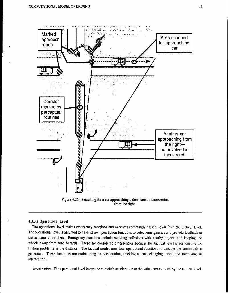
COMPUTATIONAL MODEL OF DRIVING 63
Anothreca
approachArea scannedroac for approaching
car
Corridormarked by . ....perceptual
routines ,
' ,: . .. A n o th e r c a r. ..... ,approaching from
..... " the right-~not involved in
-- ------- -this search
Figure 4.26: Searching for a car approaching a downstream intersectionfrom the right.
4.3.3.2 Operational LevelThe operational level makes emergency reactions and executes commands passed down from the tdcLical level.
The operational level is assumed to have its own perception functions to detect emergencies and provide feedback tothe actuator controllers. Emergency reactions include avoiding collisions with nearby objects and keeping thewheels away from road hazards. These are considered emergencies because the tactical level is responsible forfinding problems in the distance. The tactical model uses four operational functions to execute the commands itgenerates. These functions are maintaining an acceleration, tracking a lane, changing lanes, and travcr ng anintersection.
Acceleration. The operational level keeps the vehicle's acceleration at the value commanded by the tactical level.

64 ANNUAL REPORT 1991
Find current lane Find path in intersection
Profile road Find next car in intersection
Mark adjacent lane Find intersection roads
Track lane Find signal
Find next lane mark Find back-facing signs
Find next sign Find crossing cars
Find next car Distance between marks
Table 4.6: Perceptual routines in Ulysses.
Speed control is not used because an instantaneous change in speed requires an infinite impulse of force, while acange in acceleration requires only a step change in force. Vehicle dynamics dictate that an operational controlleris more likely to achieve the latter. The choice of control variables is not crucial to the model., However, we expectthat it might be difficult in some robot implementations to provide frequent command updates at the tactical level,so acceleration commands would prove to be more convenient.
Lane Tracking. The operational level is assumed to be able to drive the robot down a lane without interventionfrom the tactical level. This function involves only steering, as do lane changing and intersectioi travr rsl. Asdescribed earlier, the tactical level adjusts the speed independently to keep lateral accelerations within himitLs onturns.
Lane Changing. Lane changing requires the operational level to detect the adjacent lane and begin a double-curvemaneuver to move the robot over. When the robot reaches the new lane, lane tracking automatically takes over. Atmost speeds, the steering angle is adjusted to limit the robot's lateral acceleration to a safe value. This constiaintresults in a lane change maneuver that takes a roughly constant amount of time, independent of speed. The tacticallevel can use this fact to estimate the length of a lane change. However, if the robot is changing speeds (e.g.,braking while approaching an intersection), it is impossible to predict exactly how far the robot will travel during themaneuver. At low speeds, robot can only increase the steering angle to the physical stops of the vehicle. This angledetermines the minimum lane change distance for a given road width.
Intersection Traversal. Since intersections generally do not have marked lanes, the operational system is rcLmrcdto find a path to the given departure lane and chive the robot along the path. As with the other operational functions%,there are several ways this may be accomplished. We expect that the robot would follow an imaginary path createdfrom general knowledge about the size of the intersection, and then start up lane tracking when the new lane becameclearly visible.

COMPUTATIONAL MODEL OF DRIVING 65
4.3.4 SummaryUlysses is a computational model of driving implemented as a computer program. It emphasizes the tactical
level. Strategic functions are limited to providing a route plan step at every intersection. The operational level
abstractly implements tactical commands.
Ulysses can drive the robot in traffic on multi-lane roads, through intersections, or both. Driving knowledge is
encoded as constraints and preferences. Ulysses looks for lane endings, curves, speed limit signs, and other cars to
constrain the robot's acceleration on a road. When approaching an intersection, the program directs the perception
subsystem to look for signs, signals, markings, other roads, and approaching traffic as well as the general road
features just mentioned. Ulysses determines the semantics of the traffic control devices and the road configuration
and decides whether the robot has the right of way to enter the intersection. Stop signs and conflicting traffic causethe robot stop and then enter a waiting state until traffic clears or the signal changes. The program also evaluates
lane channelization, potential speed increases in adjacent lanes, traffic in adjacent lanes, and lane position to decidewhether the robot should change lanes. Additional acceleration constraints prevent the robot from approaching theintersection in the wrong lane or in the middle of changing lanes.
Ulysses uses demand-driven perception. The robot looks at the world frequently so that it can respond qaick I" 0
changing traffic situations. The model uses perceptual routines and visual markers to find trallic% object,, with the'
appropriate spatial relationships to the robot.
4.4 The PHAROS Traffic SimulatorOur motivation for creating a driving model was to describe how to drive an autonomous vehicle. Actually
driving a vehicle requires that the driving model be made concrete. The model must specify how all knowledge isencoded and how information is processed. In the preceding section we described how this is done in our model.
However, the proof of the pudding is in the eating- descriptions cannot drive real vehicles. Our first step towardusing our model on a real robot has been to implement the model in a computer program, Ulysses, and drive asimulated robot in a simulated traffic environment. PHAROS is the traffic simulator we developed for this work.
There are several advantages to driving in simulation before trying tL drive an actual vehicle. First, a simulator is
flexible. It is possible to generate almost any traffic situation to test various kinds of driving knowledge. Thesesituations can be recreated at will to observe how new driving knowledge changes a vehicle's behavior. Simulators
are also convenient, because simulated driving is not dependent on working vehicle hardware, convenient test sites,
or weather, Finally, simulated driving is safe and avoids the problem of placing other drivers at risk while testing
the robot.
Figure 4.27 shows how ,"-AROS and Ulysses work together. PHAROS maintains a database describing the
street environment and records for each car. PHAROS also controls the behavior of the simulated cars, which wecall zombies., The simulator executes a decision procedure for each zombie to determine its actions, and then 1ot\ Q,,
it along the street. A robot is simulated by replacing the decision procedure with an interface to Ulysses. Ulvy',.sruns as a separate program-sometimes on a different computer-and gets perceptual information by sending
requests to PHAROS. The interface simulates the perceptual routines described earlier Alter Ulysscs ha the
information it needs, it sends commands through the interface to the vehicle record. PHAROS then moves the robotusing the normal movement routine. The requests for (simulated) perception and the commands for (simulatCd)
control are the only communications between Ulysses and PHAROS., This arrangement ensures that Ulysses cannot
"cheat" by examining the internal state of the simulator.
The remainder of this section discusses the representation of the street environment, the driving decisions made
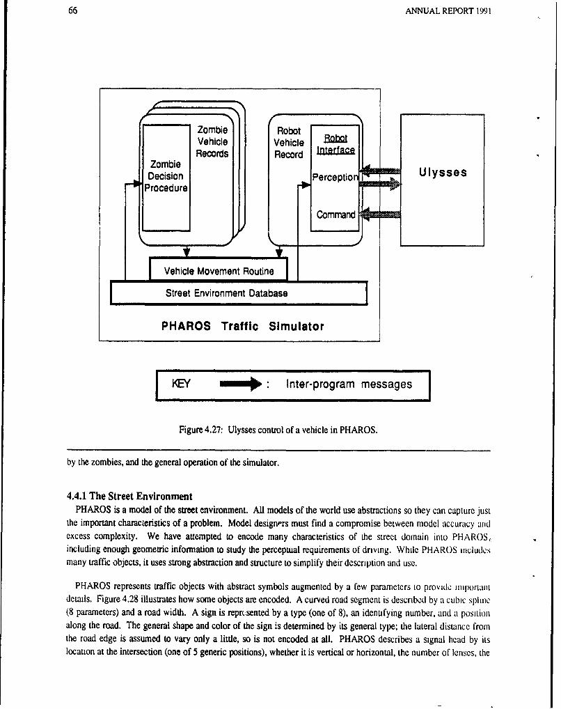
66 ANNUAL REPORT 1991
lZombie RobotVehicle Vehicle RotRecords Record
Zombie
Decision Perception q = Ulysses-IProcedure m
Command 00 on
V cMovement Routine
Street Environment Database
PHAROS Traffic Simulator
KEY mom+ Inter-program messages I
Figure 4.27: Ulysses control of a vehicle in PHAROS.
by the zombies, and the general operation of the simulator.
4.4.1 The Street EnvironmentPHAROS is a model of the street environment. All models of the world use abstractions so they can capture just
the important characteristics of a problem. Model design-rs must find a compromise between model accuracy anidexcess complexity. We have attempted to encode many characteristics of the street domain into PHAROS,including enough geometric information to study the perceptual requirements of driving. While PHAROS includesmany traffic objects, it uses strong abstraction and structure to simplify their description and use.
PHAROS represents traffic objects with abstract symbols augmented by a few parameters to provide importantdetails. Figure 4.28 illustrates how some objects are encoded. A curved road segment is described by a cubic spline(8 parameters) and a road width. A sign is repr(:sented by a type (one of 8), an identifying number, and a positionalong the road. The general shape and color of the sign is determined by its general type; the lateral distance fromthe road edge is assumed to vary only a little, so is not encoded at all. PHAROS describes a signal head by itslocation at the intersection (one of 5 generic positions), whether it is vertical or horizontal, the number of lenses, the

COMPUTATIONAL MODEL OF DRIVING 67
Symbol Example Parameters
RoadSegment Width CurvedlStraight Cubic spline paramters
Sign Identification # Type Position
Q STOP
V YIELD-E Regulatory
~Warning
<> ConstructionSGuideE1
r-J Service
EL Recreation
Signal Head Location Orientation # Lenses Lens symbol Lens color
0 RedYellow
or Green
(or
combination)
Figure 4.28: Examples of traffic object encodings.
symbols on the lenses, and the color of the lenses.
PHAROS groups traffic object symbols into structures to give them meaning for driving. It would be dittlicult todetermine how streets connected or whether a car could move to an adjacent lane if the lane and line objects in thedatabase were not organized. PHAROS connects objects to one another to form hierarchies and networks ol relatedobjects. Figure 4.29 shows how different street objects are connected to one another.,
The abstraction and structure used in PHAROS limit the accuracy with which it can simulate the world Forexample, PHAROS cannot easily simulate roads without marked lanes. PHAROS vehicles cannot abandon the lane
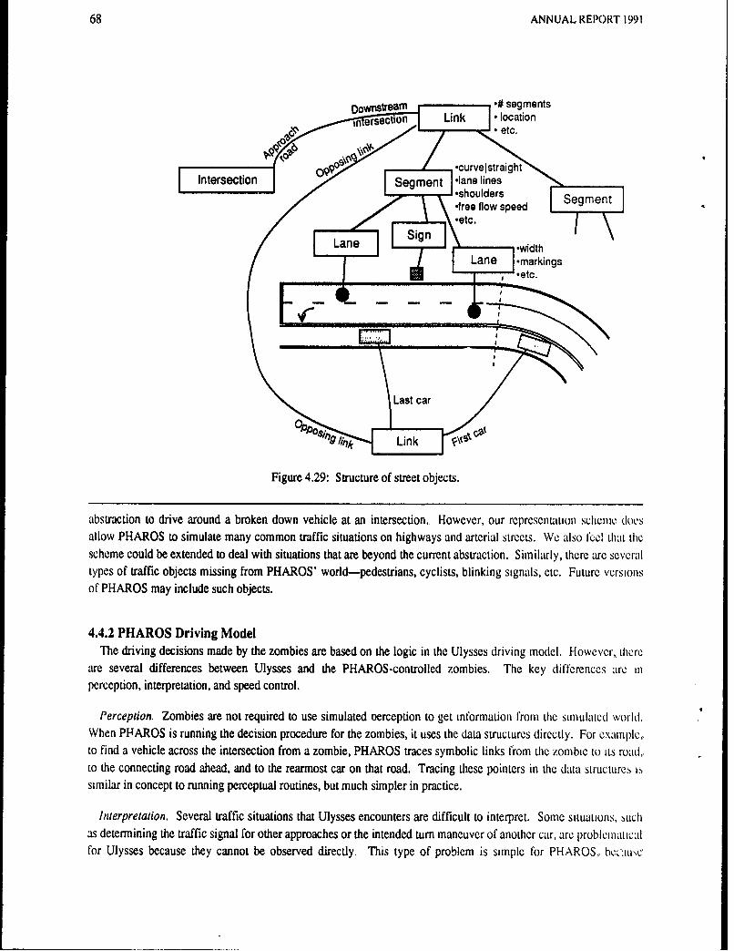
68 ANNUAL REPORT 1991
Downstream # segments' °in er' ' sc " o" Link , I ocation
I , n t e s e t o n S e g m e n t •~h u d r e mfree flow speed Segment
Lane Swidth
Lane -markings
'etc.
~Last car
Link
Figure 4.29: Structure of street objects.
abstraction to drive around a broken down vehicle at an intersection., However, our representation scheme doesallow PHAROS to simulate many common traffic situations on highways and arterial streets. We also feel that thescheme could be extended to deal with situations that are beyond the current abstraction. Similarly, there are severaltypes of traffic objects missing from PHAROS' world---pedestrians, cyclists, blinking signals, etc. Future versionsof PHAROS may include such objects.
4.4.2 PHAROS Driving ModelThe driving decisions made by the zombies are based on the logic in the Ulysses driving model. However, there
are several differences between Ulysses and the PHAROS-controlled zombies. The key differences are inperception, interpretation, and speed control.
Perception. Zombies are not required to use simulated oerception to get information from the simulated world.When P1-AROS is running the decision procedure for the zombies, it uses the data structures directly. For example,to find a vehicle across the intersection from a zombie, PHAROS traces symbolic links from the zombie to its road,to the connecting road ahead, and to the rearmost car on that road. Tracing these pointers in the data structures issimilar in concept to running perceptual routines, but much simpler in practice.
Interpretation. Several traffic situations that Ulysses encounters are difficult to interpret. Some situations, suchas determining the traffic signal for other approaches or the intended turn maneuver of another car, are problcmaticalfor Ulysses because they cannot be observed direcdy. This type of problem is simple for PHAROS, bcQ':u,,c

COMPUTATIONAL MODEL OF DRIVING 69
zombies have access to the entire database and are not limited by what they can see. This access extends even toexamining the internal state of other zombies. Other situations, such as deciding which signal head applies to therobot's lane, require several observations followed by a reasoned guess. Some situations are complex enough thatwe cannot yet describe how to recognize them. For example, we stated earlier that Ulysses cannot tell whether ablocking car in front of the robot is really broken down or merely part of a queue that extends to the intersection.
PHAROS shortcuts these difficult interpretation problems by encoding the semantics of situations directly into thedatabase. For example, the traffic control for each lane is provided as part of the input data for the simulation and isstored with the other characteristics of the street. Lane channelization is also provided externally and stored.Zombies determine if the car in front of them is in a queue simply by checking that car's "Queue" status; a zombiesets its own status to "enqueued" if it is close to the car in front and the car in front is already in a queue., The directencoding of interpreted information, as well as the availability of physically unobservable state information, allowsPHAROS to move zombies realistically witiout the complete expertise of a human driver.
Speed control. PHAROS drivers are allowed perfect perception and access to special information so that they canchoose actions as realistically-i.e., with human competence-as possible. However, zombies behaveunrealistically if they are allowed to control speed too well. Therefore, PHAROS incorporates a reaction delay intozombie speed control. When zombies wish to decelerate quickly, they must switch to a braking "pedll" (strte), indwhen they wish to accelerate again they must switch to an accelerator "pedal." There is a delay of ).8 s, on avmge,in switching between pedals. This imposed reaction delay, when combined with the car-following law aheadydiscussed, results in fairly realistic behavior during car following, free-flow to car following transitions, free-flow 1o
enqueued transitions, and queue discharge.
4.4.3 Simulator FeaturesInput., PHAROS generates a street database from a data file that it reads in at the start of each simulator run.
Since PHAROS can represent a lot of detail in a variety of traffic objects, the data file can be fairly complex. ThePHAROS user must encode the desired street environment into symbols and numbers and type them into the Iilt.Figure 4.30 shows an example of how one face of a traffic signal head is encoded. The terms "face" and "lens" ai
face vertical 5 L9 LEFT MARGIF 0 0lens RED SIGNAL SC SOLID 8 1 1 1 1 0 0 1lens AMBER SIGNAL SE SOLID 8 0 0 0 0 0 0 1 0lens GREEN SIGNAL SC SOLID 8 0 0 0 0 0 1 0 0lens AMBER-SIGNAL SCLEFT TURN 8 0 0 0 0 1 G 0 0lens GREEN-SIGNAL SC-LEFT-TURN 8 0 0 0 1 0 0 0 0
Figure 4.30: Example of signal head encoding in PHAROS data file.
keywords. The first line indicates that there are 5 lenses on this face of the signal head, that they are arrangedvertically, and that the head is located on the left shoulder of the street named "L9." If the head were directl) ovei alane, the last two numbers on the first line would indicate which lane and where along the lane the head was latLedThe remaining lines describe each lens. The information includes the color, symbol, and diameter o1 the lcen, ,indwhether the lens is lit in each phase.
Encoding and typing this information is tedious and error-prone for multi-intersection networks. A Iutie \ crsionof PHAROS should include a graphical input interface that generates the file automatically from pictorialdescriptions.
Time., PHAROS has features of both a discrete time and a discrete event simulator. Some events, such as zombiecreation and traffic signal changing, happen at irregular intervals; others, such as updating the positions of x'ele,

70 ANNUAL REPORT 1991
occur at regular intervals. PHAROS maintains an event queue that keeps track of both types of events. Theposition-update events compute the vehicles' new positions exactly from their (constant) accelerations over thepreceding time interval.
Display and user interaction. The output of PHAROS is an overhead view of the street environment with ananimated display of the vehicles. This graphical output provides us with our primary means of evaluating thebehavior of both zombies and robots. Figure 4.31 is a picture of the computer screen while PHAROS is running.
isplay Interval, w OTIt to
Tr €fi Simlator
Carnhgis Mula Univerel ty, 1905
Figure 4.31: The output display of PHAROS.
The figure shows a black-and-white approximation of the computer's high-quality color display. In the lower-leftcomer is a window showing the entire street network schematically. A portion of the network (enclosed by a smallrectangle in the schematic) is drawn at larger scale in the top-center of the screen. Cars are visible as whiterectangles, with dark regions at the rear showing brake lights and directional signals. The small window to the rightof the network schematic shows simulator time. A user can interactively pan and zoom around the streets toexamine various areas in more detail. It is also possible to select individual zombies and trace their decisionprocesses. The simulator can be paused or stepped one decision cycle (100 ms) at a time.
To simulate a robot, a user selects the "button" on the screen marked "create;" PHAROS then pauses and askswhere the robot should be injected into the street network. The robot is rendered in a unique color., We have created

COMPUTATIONAL MODEL OF DRIVING 71
various displays to study the activity of Ulysses, including the location of each mark created by the perceptualroutines, a count of the number of perceptual requests, and a chart of perceptual activity in each direction.
Performance. The simulator is written in C and runs on a Sun workstation under Sunview. A Sun 4/40 can drive
about 30 zombies 3 times faster than real time. With Ulysses driving a robot, the simulation runs much slower thanreal time. The slowdown is due to the large number of messages that must be passed between the Ulysses andPHAROS and the frequent switching of control between the programs.
PHAROS has be invaluable for us in our research on :obot driving. It allows us to test driving decision
procedures and examine perception and information flow in Ulysses. PHAROS has been sent to several other sites
doing research in driving, robotics, and artificial intelligence.
4.5 ConclusionsResearch in autonomous vehicle technology in the past 30 years has provided vehicles that can competently
perform operational driving tasks. Although computers can also plan errands and find routes, they cannot make theimmediate decisions necessary to drive in traffic. Ulysses is a model for driving that describes how to perform thesetactical tasks. Ulysses incorporates driving knowledge that describes how various traffic objects and situationsconstrain a vehicle's actions. This knowledge recognizes situations from specific relations among physical objects.Ulysses includes tactical perceptual routines for finding these objects in the world and relating them to the vehicle.
The model is implemented as a computer program so that it may be developed and tested objectively; it is currently
used to drive a robot in the simulated world of PHAROS.,
Ulysses was designed to drive safely in the PHAROS world. Our goal was to prevent the simulated robot fromhaving or causing accidents, and from unnecessarily constraining itself to stop. We have achieved this goal fbr
several traffic situations, including different types of intersections, multiple lane roads, and freeway interchangeswith light traffic. Future improvements to Ulysses might include new behaviors such as overtaking, improvedmerging, or "edging" into an intersection while waiting for a gap. A more significant improvement in driving
knowledge that we have not yet examined closely is the analysis of nearby traffic to predict how other cars will
move. Tb; analysis would involve the detection of many other cars, the abstraction the relative motions of the cars,and the projection of the motions into the future. Eventually the model must be combined with a strategic drivingprogram; the parameters in Ulysses would then be determined by variable strategic goals, such as time stress,
pleasure in driving, worry about citations, fuel efficiency, etc. PHAROS and Ulysses could also be expanded toinclude more objects such as blinking signals, activated signals, bicycles, pedestrians, roads without lanes, and
different vehicle types.
Rather than adding more sophisticated driving knowledge, our more immediate goal is to determine how a realrobot can perform the basic tactical tasks. As Ulysses drives a robot in PHAROS, it generates many perceptualrequests. Machine perception is very expensive computationally, so it is important to find ways to minimize the cost
of the requests. We are studying ways to take advantage of the coherence of situations over time and the differencein criticality of constraints to eliminate unnecessary requests. In the future we will study how a resource-limited
robot might choose the best perception and constraint-generation actions to perform when it cannot perform themall.. We would also like to model uncertainty in sensing and interpretation explicitly, and empower Ulysses tochoose actions with the maximum expected utility. Finally, a truly intelligent driving model should be able to learnhow to improve :.t behavior as it gains experience driving.
Ulysses has four major strengths as a driving model: it comprises many driving tasks; it models individualdrivers; it is grounded in (perceived) physical objects and operational maneuvers; and it specifies how to computeactions from perceptions. Of these characteristics, physical grounding and explicit computation are probably the

72 ANNUAL REPORT 1991
most importanL They allow the model to be designed and used objectively, independent of human interpretation, Acomputational model can help to detect problems that human designers may not see. For example, we described
earlier how Ulysses looks at the backs of Stop signs facing the cars on cross streets. We did ri.t plan to include sucha perceptual action in Ulysses, but after the intersection rules were encoded it became clear that this information isnecessary for determining right of way. None of the driving task descriptions we studied-including the McKnightanalysis [26], and the official driver's manual [8] and vehicle code [25] for our state-call for this action. A modelsuch as Ulysses can predict a driver's real information needs in any situation.
The characteristics described above ma~e Ulysses uniquely suitable for driv. e an autonomous vehicle. Theyalso give Ulysses the potential to contribute to general driving research. Reseor q in driving seeks to answer manyquestions that apply equally to a robot and human driver, such as "How can a chiver learn to make better decisions?"and "what information should be provided along roads to make driving easier"' We can answer these questions ifwe have an accurate, concrete driver model. We feel that computational driver models will prove to be invaluabletools for driving research.
COMPUTATIONAL MODEL Of DRIVING 73
References
[I] Aasman, Jans.Implementations of Car-Driver Behaviour and Psychological Risk Models.In J. A. Rothengatter and R. A. deBruin (editors), Road User Behaviour: Theory and Practice, pages
106-118. Van Gorcum, Assen, 1988.
[2] Agre, P. E. and D. Chapman.Pengi: An Implementation of a Theory of Activity.In Proceedings of the Sixth National Conference on Artificial Intelligence, pages 268-272. Morgan Kaufman
Publishers, Los Altos, 1987,
[3] Belcher, P. L. and Caftling, I.Autoguide Electronic Route Guidance in London and the U.K..Technical Report 89102, ISATA, June, 1989.
[4] Bender, J. G. and Fenton, R. E.A Study of Automatic Car Following.IEEE Transactions on Vehicular Technology VT-18:134 - 140, Nov., 1969.
[5] Cardew, K. H. F.The Automatic Steering of Vehicles -- An Experimental System Fitted to a Citroen Car.,Technical Report RL 340, Road Research Laboratory, February, 1970.
[6] Chin, H.C.SIMRO: A Model To Simulate Traffic at Roundabouts.Traffic Engineering and Control 26(3), March, 1985.
[7] Cro, J. W. and Parkr, R. H.Automatic Headway Control -- An Automobile Vehicle Spacing System.Technical Report 700086, Society of Automotive Engineers, January, 1970.
[8] Department of Transportation.Pennsylvania Manual for Drivers (Publication 95)Commonwealth of Pennsylvania, Harrisburg, PA, 1984.
[9] Dickmanns, E. and Zapp, A.A Curvature-Based Scheme for Improving Road Vehicle Guidance by Computer Vision.In Mobile Robots (Vol. 727). SPIE, 1986.
[10] Drew, Donald.Traffic Flow Theory and Control.McGraw-Hill Book Company, New York, 1968.
[11] Elliott, R. J. and Lesk, M. E.Route Finding in Street Maps by Computers and People.In Proceedings of AAA/ 82, pages 258- 261. AAAI, 1982.
[12] FHWA.Traffic Network Analysis with NETSIM: A User GuideFederal Highway Administration, Washington, D.C., 1980.
[13] Fenton, R. and Mayhan, R.Autemated Highway Studies at the Ohio State University -- An Overview.IEEE Transactions on Vehicular Technology 40(1):100 - 113, February, 1991..
[14] Gage, D. W. and Pletta, B. J.Ground Vehicle Convoying.In Mobile Robots 1 (Vol. 852), pages 319 - 328. SPIE, 1987.
[151 Gardels, K.Automatic Car Controls For Electronic Highways.Technical Report GMR-276, General Motors Research Labs, Warren, MI, June, 1960.
74 ANUAL REPORT 1991
[16] Gibson, D. R. P.Available Computer Models for Traffic Operations Analysis.In The Application of Traffic Simulation Models. TRB Special Report 194., pages 12 - 22. National
Academy of Sciences, 1981.
[17] Hayes-Roth, B.A Blackboard Architecture for Control.Artificial Intelligence 26:251 - 321, 1985.
[18] Kawashima, H.Two Major Progiam Demonstrations in Japan.IEEE Transactions on Vehicular Technology 40(1):141 - 146, February, 1991.
[191 Kehtarnavaz, N., Lee, J. S., and Griswold, N. C.Vision-Based Convoy Following by Recursive Filtering.
[20] Kluge, K. and C. Thorpe.Explicit Models for Road Following.In Proceedings of the IEEE Conference on Robotics and Automation. IEEE, 1989.
[21] Kories, R., Rehfeld, N. and Zimmermann, G.Toward Autonomous Convoy Driving: Recognizing the Starting Vehicle in Front.In Proceedings of the 9th International Conference on Pattern Recognition, pages 531 - 535. IEEE, 1988.
[22] Kuan, D., Phipps, G, and Hsueh, A-C.Autonomous Robotic Vehicle Road Following.IEEE Transactions on PAMI 10(5):648 - 658, 1988.
[23] Laird, John E; Newell, Allen; and Rosenbloom, Paul S.Soar: an Architecture for General Intelligence.Artificial Intelligence 33:1 -64, 1987.
[24] Lang, R. P. and Focitag, D. B.Programmable Digital Vehicle Control System.IEEE Transactions on Vehicular Technology VT-28:80 -87, Feb, 1979,
[25] Legislative Reference Bureau.Pennsylvania Consolidated Statutes, Title 75: Vehicles (Vehicle Code)Commonwealth of Pennsylvania, Harrisburg, PA, 1987..
[261 McKnight, J. and B. Adams.Driver Education and Task Analysis Volume I: Task Descriptions.Final Report, Department of Transportation, National Highway Safety Bureau, Washington, D.C.,
November, 1970.
[27] Michon, J. A.A Critical View of Driver Behavior Models: What Do We Know, What Should We Do?In L. Evans and R. Schwing (editors), Human Behavior and Traffic Safety. Plenum, 1985.
[28] Oshima, R. et al.Control System for Automobile Driving.In Proceedings of the Tokyo IFAC Symposium, pages 347 - 357.. , 1965..
[29] Pomerleau, D. A.ALVINN: An Autonomous Land Vehicle In a Neural Network.Technical Report CMU-CS-89-107, Carnegie Mellon University, 1989.
[301 Reece, D. A. and S. Shafer.An Overview of the Pharos Traffic Simulator.Jn 1. A. Rothengatter and R. A. deBruin (editors), Road User Behaviour: Theory and Practice. Van Gorcum,.
Assen, 1988.

COMPUTATIONAL MODEL OF DRIVING 75
[31] Reid, L. D.; Graf, W. 0.; and Billing, A. M.The Validation of a Linear Driver Model.Technical Report 245, UTIAS, March, 1980.
[32] Rillings, J. H. and Betsold, R. J.Advanced Driver Information Systems.IEEE Transactions on Vehicular Technology 40(1), February, 1991.
[33) T. Rothengatter and R. de Bruin (editor).Road User Behaviour.Van Gorcum, 1988.
[34] Shladover, S. E. et al.Automatic Vehicle Cona'ol Developments in the PATH Program.IEEE Transactions on Vehicular Technology 40(1): 114 - 130, Feb, 1991,
[35] Sugie, M., Menzilcioglu, 0., and Kung, H. T.CARGuide -- On-board Computer for Automobi,, Route Guidance.,Technical Report CMU-CS-84-144, Carnegie Mellon University, 1984.
[36] Texas Engineering Experiment Station.BART. Binocular Autonomous Research Team.Research brochure, Texas A&M University.1989
[37] Thorpe, C., Hebert, M., Kanade, T., and Shafer, S.Vision and Navigation for the Carnegie Mellon NAVLAB.IEEE Transactions on PAMI 10(3), 1988.
[38] Tsugawa, S., Yatabe, T., Hirese, T., and Matsumoto, S.An Automobile with Artificial Intelligence.In Proceedings of the 6th IJCAI, pages 893 -895, UCAI, 1979.
[391 Turk, M., Morgenthaler, D., Gremban, K., and Marra, M.Video Road-Following for the Autonomous Land Vehicle.In Proceedings of the International Conference on Robotics and Automation. IEEE, 1987.
[40] van der Molen, H.H., and Botticher, A.M.T.Risk Models for Traffic Participants: A Concerted Effort for Theoretical Operationalizations.Road Users and Traffic Safety.In J. A. Rothengatter and R. A. de Bruin,Van Gorcum, Assen/Maastricht, The Netherlands, 1987, pages 61-82.
[41] von Tomkewitsch, R.Dynamic Route Guidance and Interactive Transport Management with ALl-Scout.IEEE Transactions on Vehicular Technology 40(1):45 - 50, February, 1991..
[42] Waxman, Allen; LeMoigae, Jacqueline J; Davis, Larry S.; Slinivasan, Babu; Kushner, Todd R.; Liang, Eliand Siddalingaish, Tharakesh.A Visual Navigation System for Autonomous Land Vehicles.IEEE Journal of Robotics and Automation RA-3(2), April, 1987.
[4 ,J Wong, Shui-Ying.TRAF-NETSIM: How It Works, What It Does.ITE Jourial 60(4):22 - 27, April, 1990.

76 ANNUAL REPORT 1991

NEURAL NETS AND SYMBOLS 77
5. Combining artificial neural networks and symbolic processing for autonomousrobot guidance
5.1 IntroductionArtificial neural networks are commonly employed as monolithic non-linear classifiers. 1 The technique, often
used in domains such as speech, character and target recognition, is to train a single network to classify inputpatterns by showing it many examples from numerous classes. The mapping function from inputs to outputs in
these classification tasks can be extremely complex, resulting in slow learning and unintelligible internalrepresentations.
However there is an allnative to this monolithic network approach. By training multiple networks on different
aspects of the task, each can learn relatively quickly to become an expert in its sub-domain. This chapter describes atechnique we have developed to quickly train expert networks for vision-based autonomous vehicle control., Usingthis technique, specialized networks can be trained in under five minutes to drive in situations such as single-laneroad driving, highway driving, and collision avoidance.
Achieving full autonomy requires not only the ability to train incvidual expert networks, but also the ability tointegrate their responses. This chapter focuses on rule-based arbitr ition techniques for combining muluple dri\ ingexperts into a syst.;m triac is capable of guiding a vehicle in a variety of circumstances. These techniques arccompared with .ither neural network integration schemes and shown to have a distinct advantage in donains wheresymbolic knowledge and techniques can be employed in the arbitration process.
5.2 Driving Module ArchitectureThe architecture for an individual ALVINN driving module is shown in Figure 5.2. The input layer consists of a
single 30x32 unit "retina" onto which a sensor image fiom either the video camera or the laser range finder isprojected. Each of the 960 input units is fully connected to the hidden layer of 5 units, which is in turn fullyconnected to the output layer. The 30 unit output layer is a linear representation of the currently appropriate steeringdirection. The centermost output unit represents the "travel straight ahead" condition, while units to the left andright of center represent successivei, sharper left and right turns. The steering direction dictated by the net\\orkmay serve to keep the vehicle on the road or to prevent it from colliding with nearby obstacles, depending on thetype of sensor input and the driving situation the network has been trained to handle.
To drive the N: vlab, an image from the appropriate sensor is reduced to 30 x 32 pixels and projected onto theinput layer.. Aiter l.ropagating activation through the network, the output layer's activation profile is translated intoa vehicle steering cornmand. The steering direction dictated by the network is taken to be the center of mass of the"hill" of activation surrounding the output unit with the highest activation level. Using the center of mass olactivation instead of the most active output unit when determining the direction to steer permits finer stecringcorrections, thus improving ALVINN's driving accuracy.,
1A previous version of this chapter is accepted for publication in the Journal of Engineenng Applications of Artificial intelficnmc, %tILh thQsame title, authored by Dean Pomerleau, Jay Gowdy, and Charles Thorpe

78 ANNUAL REPORT 1991
Slop 5tSbi;f 30output
U Units
( i 5 Hidden
Units
30x32 SensorInput Retina
Figure 5.1: The architecture for an individual ALVINN driving module
5.3 Individual Driving Module Training And PerformanceWe have developed a scheme called training "on-the-fly" to quickly teach individual modules to imitate thc
driving reactions of a person. As a person drives, the network is trained with back-propagation using the latest videocamera image as input and the person's current steering direction as the desired output. To facilitate genera fizationto new situations, additional variety is added to the training exemplars by shifting and rotating the original caneraimage in software to make it appear that the vehicle is situated differently relative to the environment (See Figure5.3). The correct steering direction as dictated by the driver for the oiginal image is altered for each oi the
Shifted and Rotated Images
Figure 5.2: The single original video image is shifted and rotated to create multiple training exemplars in whichthe vehicle appears to be at a different locations relative to the road.

NEURAL NETS AND SYMBOLS 79
transformed images to account for the altered vehicle placement. Adding these transformed patterns to the trainingset allows the network to learn to recover from driving mistakes, without requiring the human trainer to explicitlystray from the road center and then return. For more details about the technique and purpose of training on-the-fly,see [7].
Running on three Sun-4 Sparcstations, training on-the-fly requires about five minutes during which a persondrives the Navlab at about six miles per hour over a 1/4 to 1/2 mile stretch of training road. Once it has learned, thenetwork can accurately traverse the length of road used for training and also generalize to drive along parts of theroad it has never encountered under a triety of weather conditions. In addition, since determining the steeringdirection from the input image merely involves a forward sweep through the network, the system is able to process20 images per second, allowing it to drive at up to the Nhvlab's maximum speed of 20 miles per hourfoomnote(TheNavlab has a hydraulic drive system that allows for very precise speed control, but that prevents the vehicle fromdriving over 20 miles per hour.). This is over twice as fast as any other sensor-based autonomous system has driventhe Navlab [6, 3].
Figure 5.3: Video images taken on three of the roads ALVINN modules have been trained to handle. They are,from left to right, a single-lane dirt access road, a single-lane paved bicycle path, and a lincdtwo-lane highway.
The flexibility provided by training on-the-fly has facilitated the development of individual driving networks tohandle numerous situations. Using video camera images as input, networks have been trained to drive on single-lane dirt roads, single-lane paved roads, two-lane suburban neighborhood streets, and lined two-lane highways (SecFigure 5.3),
By replacing the video input with alternative sensor modalities, ALVINN has learned other interesting behaviors.One such sensor onboard the Navlab is a scanning laser range finder., The range finder provides images in whichpixel values represent the distance from the range finder to khe corresponding area in the scene., Obstacles such astrees and cars appear as discontinuities in depth, as can be seen in the simulated range finder image at the bottom ofFigure 5.3. Using this sensor, separate ALVINN modules have been trained to avoid collisions in obstacle-richenvironments and to follow alongside rows of parked cars.
A third type of image used as input to ALVINN modules comes from a laser reflectance sensor, In this type ofimage, a pixel's value corresponds to the amount of laser light that reflects off the corresponding point in the sceneand back to the sensor. The road and off-road regions reflect differently, making them distinguishable in the image(see Figure 5.3). Laser reflectance images in many ways resemble black and white video images, but have theadvantage of being independent of ambient lighting conditions. Using this sensor modality, we have trained anetwork to follow single-lane roads in total darkness.

80 ANNUAL REPORT 1991
Figure 5.4: Images taken of a scene using the three sensor modalities the system employs as input. From left toright they are a video image, a laser range finder image and a laser reflectance image. Obstacles liketrees appear as discontinuities in laser range images. The road and the grass reflect differentamounts of laser light, making them distinguishable in laser reflectance images.
5.4 Symbolic Knowledge And ReasoningDespite the variety of capabilities exhibited by individual driving networks, until recently the system nas been far
from truly autonomous. First, the one driving network architecture shown in Figure 5.2 was capable of driving onlyon the type of road on which it was trained. If the road characteristics changed, ALVINN would often becomeconfused and stray from the road. In addition, a real autonomous system needs to be capable of planning andtraversing a route to a goal. The neural network driving modules are good at reactive tasks such as road followingand obstacle avoidance, but the networks have a limited capability for the symbolic tasks necessary lor alautonomous mission. The system of networks cannot decide to turn left at an intersection in order to reach a goal.After making a turn from a one lane road to a two lane road, the system does not know that it should stop listeningto one network and start listening to another. Just as a human needs symbolic reasoning to guide reactive processes,the networks need a source of symbolic knowledge to plan and execute a mission.
Ideally, the symbolic knowledge source would reason like a person. It would use its knowledge of the world toplan a sequence of observations and corresponding actions to traverse the route. For instance, to achieve the goal ofreaching a friend's house, the mission description might be a sequences like, "Drive until the sign for Scncca Roadis seen, and turn left at that intersection. Then drive until the third house on the left is seen, and stop in front of it."
In this ideal system, once the mission is planned, the symbolic knowledge source would rely entrcl) onperception to control the execution of the mission. In other words, the symbolic resource module would be able torecognize events and use what it sees to guide the interaction of the networks. The symbolic resource module wouldbe capable of reading the street sign at an intersection and making the appropriate turn to continue on to itsdestination. It would also be able to identify the new road type and choose the appropriate network for driving onthat kind of road. Unfortunately, the perception capabilities required by such a module are beyond the current stateof the art.
In order to bridge the gap between mission requirements and perception capabilities, we use additional geometricand symbolic information stored in an "annotated map". An annotated map is a two dimensional data structurecontaining geometrical information about the area to be traversed, such as the locations of roads and landmarks, Inaddition, each object in the map can be annotated with extra information to be interpreted by the clients that accssthe map. For example, as far as the annotated map is concerned, a mailbox is simply a two dimensional polygon, at aparticular location with some extra bits associated with it. The "extra bits" might represent the three dimensionalshape of the the mailbox, cr even the name of the person who owns it. The module which manages the annotatedmap does not interpret this extra information, but rather provides a mechanism for client modules to access the

NEURAL NETS AND SYMBOLS 81
annotations. This reduces the knowledge bottleneck that can develop in large, completely centralized systems.
The annotated map is not just a passive geometric database, but instead is an active part of our system., Besideshaving a 2D representation of the physical objects in a region, annotated maps can contain what are called alarms.Alarms are conceptual objects in the map, and can be lines, circles, or regions. Each alarm is annotated with a list o(client modules to notify and the information to send to each when the alarm is triggered. When the annotated mapmanager notices that the vehicle is crossing an alarm on the map, it sends the information to the pertinent modules.Once again, the map manager does not interpret the information: that is up to the client modules.
Alarms can be thought of as positionally based production rules. Instead of using perception based productionrules like, "If A is observed, then perfonp action B", an annotated map based system has rules of the form, "Iflocation A is rached, then perform action B". Thus we reduce the problem of making high lev-l decisions from thedifficult task cf peiceiving and reacting to external events to the relatively simple task of monitoring and updatingthe vehicle's position.
The first step in building an annotated map is collecting geometric information about the environment. We buildour maps by driving the vehicle over roads and linking the road segments together at intersections. At the samctime, a laser range finder is used to record the positions of landmarks such as mailboxes and telephone poles.Planning a particular mission requires adding specific instructions to the map in the form of "trigger annotations".This is currently a process performed by the person planning the mission. For example, the human expert knowsthat when approaching an intersection, the vehicle should slow down, so the expert chooses the appropriate locationto put the trigger line. The trigger line goes across the road at that point, and is annotated with a string of bits thatrepresents the new speed of the vehicle. During the run, when the vehicle crosses the trigger line, the map managersends the string of bits to a module that interprets the information and slows the vehicle to the desired speed. In thecurrent system, alarms are interpreted as commands, but there is no predefined "correct" way for a module to reactto an alarm. Depending on its content, an alarm could also be interpreted as a wakeup call, or even as simplyadvice.
Because position information is so critical to an annotated map system, we use multiple techniques to detcrminethe vehicle's current location. We use an Inertial Navigation System (INS) which can determine the vehicle'slocation with an error of approximately 1\% of distance traveled [1]. To eliminate positioning error thataccumulates over time in the INS data, the annotated map system also uses information from perception modules.For example, since the driving networks presumably keep the vehicle on the road, lateral error in die veh,.:hpositioning system relative to the road can be identified and eliminated. In addition, a modulk usin, !he ha:e' raneefinder compares the landmarks it sees to the landmarks collected when the map was built. 1mId triangula'cs thevehicle's position on the map. These techniques allow perception modules to provide useful poItiuoning in"orination
{\em without) requiring them to explicitly recognize and interpret particular objects such as street sig, Tbhposition corrections provided by perception modules are i terpreted as a change in the transform betwce-i tWlocation that the INS reports and the real vehicle position on the map. A separate module, called the navigator, is incharge of maintaining and distributing this position transform.
Annotated maps provide the system with the symbolic information and control knowledge necessary for a fullyautonomous mission. Since the control knowledge is geometrically based, and since planning is done before themission starts, runtime control comes at a low computational cost. Figure 5.4 shows the structure and interaction elthe annotated map system's components. It also illustrates the annotated map system's interaction with the othcrparts of the system, including the perceptual neural networks and the arbitrator (discussed below) Figure 5.4 sho \ Sa map and annotations for a mission segment.

82 ANNUAL REPORT 1991
EV
Tyoia
Tr~vel TraveDUCC40VS Veyum
:!Ti si~blok alpr cetal neural net wr
5.5Rul-Baed r~~in MouleLoitinWe se hesymoli kowldg prvidd y te nnoate mp sstM t epgieteinrcino h
reactie driin& h't'ralnet~ ~rks. igure5.5 sows th systm arcitetuewtmphasi MaphenualntwrsWhereas~~~~~~~~~~~~~~~~~~~~~ Fiue54sbwMdC:.~ ewr ytm nooeua c .14 "pellrceta erdntok
Fig~ .5susums he~vnctte ~ysem nt oe ackage. In this di. o'eihbo ersn.sasprproes rnnng n arii~i.~Ige fom hetheeonoai snsrsareprvi .e fvedrvig ntwi. Sow
Thge rbiTratormes of t the aneomaerice and conro inforaction rvietweby the.he annt ap ytem toperorma mssntnmouesly.c o irte vi routeo flown mul wItpin the atatdrapo swth smboic
by therou nfolwrmto cornn the direction ittinsth e i sI te ei rer to follo thde preplanned ro ute . W h eri hethe vehic e ~ is drivng d w l rdteountcfoering. Th e nu an okivng m odul, are ~ositi ns foftera ahepldcit
the vehile.BThed routen foloweruehi LgeortcLliaio ogzeatsern ietion.
Teuetesmoi nweg rvddb he annotated map system als prov gide the a.i~.rwt interaction ofabu the c~lldiigiuIin
incs udning ha tprlj ofroaues ehicle ishone and i svenso thrs arepoi '. ~cie or druin penerfk bshown
aheaitrFor xape supse duringh the plmtcannid potolifrmtoseoiddb the huaanp~notices mhta . riuap sit in ochesrfrm ison lanetooul. Thexpt woet mt foloingr mdle wth the orrespondingppoint on miuseaptan
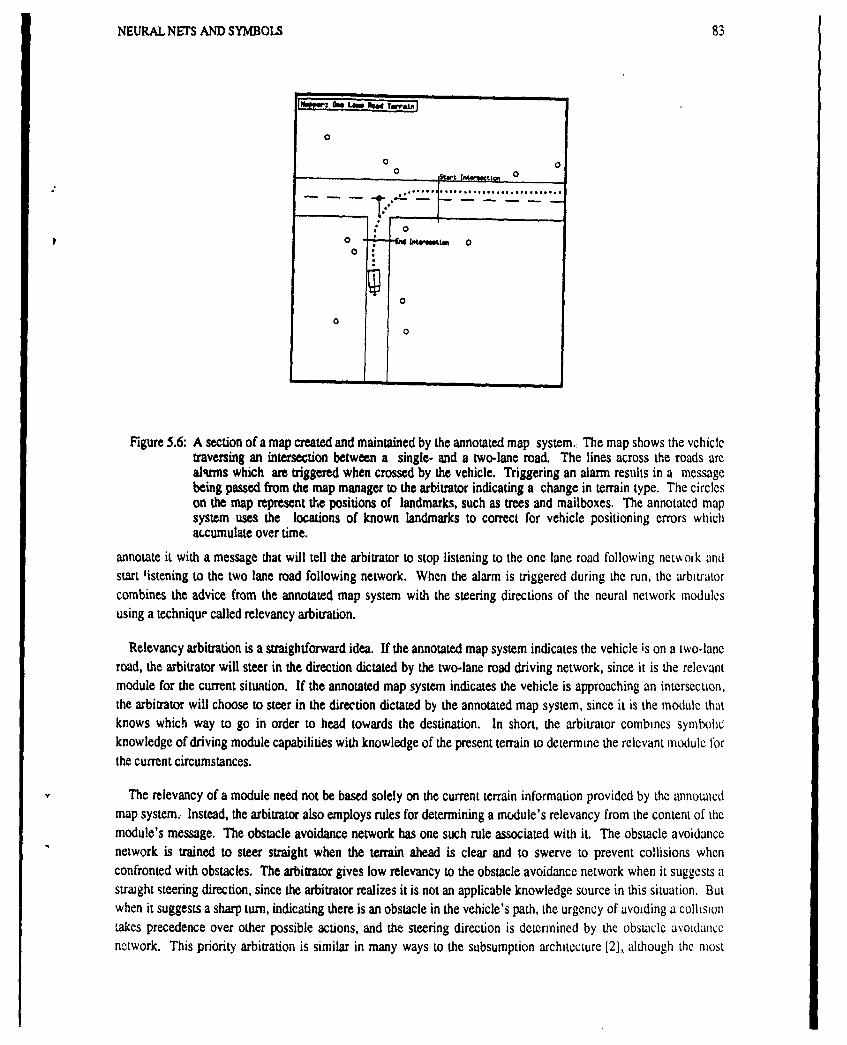
NEURAL NETS AND SYMBOLS 83
103 Ow Lam =adTuval.
0
0 i-,Urt Int ,wti., 0 01
.. ............................ese~t
0 " "rewt 00 ,
0
0o0
T" ....
Figure 5.6: A section of a map created and maintained by the annotated map system, The map shows the vehicletraversing an intersection between a single- and a two-lane road. The lines across the roads arealqrms which are triggered when crossed by the vehicle. Triggering an alarm results in a messagebeing passed from the map manager to the arbitrator indicating a change in terrain type. The circleson the map represent the positions of landmarks, such as trees and mailboxes. The annotated mapsystem uses the locations of known landmarks to correct for vehicle positioning errors whichaccumulate over time.
annotate it with a message that will tell the arbitrator to stop listening to the one lane road following netwoik andstart listening to the two lane mad following network. When the alarm is triggered during the run, the arbtratorcombines the advice from the annotated map system with the steering directions of the neural network modulesusing a technique called relevancy arbitration.
Relevancy arbitration is a straightforward idea. If the annotated map system indicates the vehicle is on a two-laneroad, the arbitrator will steer in the direction dictated by the two-lane road driving network, since it is the relevantmodule for the current situation. If the annotated map system indicates the vehicle is approaching an intersecun,the arbitrator will choose to steer in the direction dictated by the annotated map system, since it is the module thatknows which way to go in order to head towards the destination. In short, the arbitrator combines symix~icknowledge of driving module capabilities with knowledge of the present terrain to determine the relevant module forthe current circumstances.
The relevancy of a module need not be based solely on the current terrain information provided by the annotatedmap system., Instead, the arbitrator also employs rules for determining a module's relevancy from the content of themodule's message. The obstacle avoidance network has one such rule associated with it. The obstacle avoidancenetwork is trained to steer straight when the terrain ahead is clear and to swerve to prevent collisions whenconfronted with obstacles. The arbitrator gives low relevancy to the obstacle avoidance network when it suggests astraight steering direction, since the arbitrator realizes it is not an applicable knowledge source in this situation. Butwhen it suggests a sharp turn, indicating there is an obstacle in the vehicle's path, the urgency of avoiding a collisiontakes precedence over other possible actions, and the steering direction is determined by the obsucle avoidancenetwork. This priority arbitration is similar in many ways to the subsumption architecture [2], although the most

84 ANNUAL REPORT 1991
Miusi T='mm
Thwl
0. L.w To Ca. O. Lan Obi. CCWCW p YMNowak Nowagk Nowak AvoidaFo lai a ya
Ine Reflecance RangeFinderImage Im-ge
Figure 5.7: The integAied ALVINN architecture. The arbitrator uses the terrain information provided by theannotated map system as well as symbolic models of the driving networks' capabilities and prioritiesto determine the appropriate module for controlling the vehicle in the current situation.
common interaction between behaviors in Brooks' systems is for higher level behaviors to override lesssophisticated, instinctual ones.
By combining map-related knowledge about the current driving situation with knowledge about abilities andpriorities of individual driving modules, the integrated architecture provides the system with capabilities that farexceed those of individual driving modules alone. Using this architecture, the system has succe:ssfully followed a1/2 mile path through a suburban neighborhood from one specific house to another. In navigating the route, thesystem was required to drive through three intersections onto three different roads while swerving to avoid parkedcars along the way. At the end, the vehicle came to rest one meter from its destination.
5.6 Analysis And DiscussionRule-based integration of multiple expert networks has significant advantages over previously developed
connectionist arbitration schemes. One such advantage is the ease of adding new modules to the system. Usingrule-based arbitration, the new module can be trained in isolation to become an expert in a new domain, and thenintegrated by writing rules for the arbitrator which specify the new module's area of expertise and its priority. Thisis in contrast to other connectionist expert integration techniques, such as the task decomposition architecture [5],connectionist glue [81 and the meta-pi architecture (4]. To combine experts using these techniques requires thetraining of additional neural network structures, either simultaneously with the training of the experts in the case ofthe task decomposition architecture, or after expert training in the case of the connectionist glue and meta-piarchitectures. Adding a new expert using these techniques requires retraining the entire integrating structure fromscratch, which involves presenting the system patterns from each of the experts' domains, not just the new one. Thislarge scale retraining is particularly difficult in a task like autonomous navigation because it requires either drivingover all the experts' domains again, or storing a large number of domain-specific images for later reuse.

NEURAL NETS AND SYMBOLS 85
Another significant advantage of rule-based arbitration is the ease with which non-neural network knowledgesources can be integrated into the system. Symbolic tasks such as planning and reasoning about a map are currentlydifficult to implement using neural networks. In the future, it should be possible to implement more and moresymbolic processing using connectionist techniques, but until then, rule-based arbitration provides a way of bridgingthe gap between neural networks and traditional Al systems.
The technique is not without shortcomings however. The current implementation relies too heavily on theaccuracy of the annotated map system, particularly for negotiating intersections. The question might be asked, whyis the mapping system required for intersection traversal in the first place? Why can't the driving networks handle
intersections? The answer is that when approaching an intersection, an individual driving network will oftenprovide ambiguous steering commands, since there are multiple possible roads to follow. If left on its own, aroad-following network will often alternately steer towards one or the other road choices, causing the vehicle tooscillate and eventually drive off the road. In addition, even if the network could learn to definitively choose one ofthe branches to follow, it still wouldn't know which is the (\it appropriate) branch to choose in order to head towardthe destination. In short, the mapping modules can be viewed both as a useful source of high level symbolicknowledge, and as an interim solution to the difficult perceptual task of intersection navigation.,
The annotated map system as currently implemented is not a perfect solution to the problem of high levelguidance because it requires both detailed knowledge of the route, and an accurate idea of the current vehicleposition. In certain controlled circumstances, such as rural mail delivery, the same route is followed repeatedly,making an accurate map of the domain feasible. However a system capable of following less precise directions, like"go about a half mile and turn left on Seneca Road", is clearly desirable. Such a system would require morereliance on observations from perception modules and less reliance on knowledge of the vehicle's exact positionwhen making hih level decisions.
Conceptually, Liis shift towards reliance on perception for high level guidance could be done in two ways. First,observations of objects like the Seneca Road street sign, could be used to update the vehicle's position on the map.In fact, position updates based on perceptual observations are currently employed .by the annotated map systemwhen it triangulates the vehicle's location based on the positions of known landmarks in laser range images. Butposition updates are only helpful when the observations are location specific., For observations of objects like stoplights, or arbitrarily located objects like "road construction ahead" signs, the system's response should beindependent of the vehicle's location.
These location independent observations could be modeled as positionless alarms in the annotated map. When aperception module sees an object like a "road construction ahead" sign, it would notify the map manager., The mapmanager would treat the sighting as an alarm, distributing the information associated with the alarm to the pertinentmodules. Perception triggered alarms would allow the system to transition between its current perceptual abilitiesand future, more advanced capabilities.
Although the system is not yet capable of identifying and reading individual signs, we have had preliminarysuccess in using neural network perceptual observations to help guide high level reasoning. The technique relies onthe fact that when the vehicle reaches an intersection, the output of the driving network becomes ambiguous. Thisambiguity manifests itself as an output vector with more than one active steering direction corresponding to themultiple possible branches to follow. This output ambiguity has been successfully employed to update the vehicle'sposition and to follow coarse directions. As the vehicle approaches an intersection, the annotated map systemsignals the arbitrator that an intersection is coming up and that the vehicle should follow the right-hand branch inorder to head towards the goal. This level of detail does not require either a highly accurate map or preciseknowledge of the vehicle's current position. The arbitrator takes the annotated map system's message as a signal to

86 ANNUAL REPORT 1991
watch the output of the current driving network carefully. When the driving network's output becomes ambiguous,the arbitrator signals the annotated map system that the vehicle has reached the intersection and to update thevehicle's position accordingly. The arbitrator also uses the "turn right" portion of the annotated map system'smessage in order to choose the correct steering direction from the driving network's ambiguous output vector. Thiscloser interaction between the perception networks and the annotated map allows the system to use perception forintersection traversal, instead of relying solely on knowledge from the map for guidance.
Another shortcoming of rle-based arbitration as currently implemented its binary nature. Currently, a module isdeemed by the annotated map system as either appropriate or inappropriate for the current road type. This binarydecision does not address the question of intelligently combining modules trained for the same domain, such as thevideo-based single-lane driving network and the laser reflectance-based single-lane driving network. There areobviously some situations, such as night driving, when one network is better suited than the other. To take moresubtle circumstances into account when weighting the steering directions dictated by multiple networks, we aredeveloping augmented arbitration rules that consider more context than just the current road type. We are alsocurrently working on connectionist techniques that can determine a network's reliability directly from its outputalone. Preliminary results in this area look very promising.
One final drawback of the current system is the need for a human expert to preplan the mission by providing mapannotations. In the future, we will replace the humar expert with an expert system capable of annotating the mapappropriately. We understand the techniques the human expert uses to find the shortest route and to annouitc themap, so automating the process should not be difficult.
In conclusion, a modular architecture permits rapid development of expert neural networks for complex domainslike autonomous navigation. Rule-based arbitration is a simple and efficient method for combining these expertswhen symbolic knowledge is available for reasoning about their appropriateness. Rule-based arbitration alsopermits the combination of neural network experts with non-neural network processing techniques such as planning,which are difficult to integrate using other arbitration schemes.
5.7 AcknowledgementsThis work would not have been possible without the input and support provided by Dave Touretzky, John
Hampshire, and especially Omead Amidi, James Frazier and rest of the CMU ALV group.,
The principle support for the Navlab has come from DARPA, under contracts DACA76-85-C-0019,DACA76-85-C-0003 and DACA76-85-C-0002. This research was also funded in part by a grant from FujitsuCorporation.
5.8 References[1] O. Amidi and C. Thorpe.
Integrated mobile robot control.,In Proceedi',gs SPIE Mobile Robots V, pages 504-524. 1990.
[2] R.A. Brooks.A Robust Layered Control System for a Mobile Robot.IEEE Journal of Robotics and Automation RA-2(l): 14-23, April, 1986.

NEURAL NETS AND SYMBOLS 87
[3] Jill D. Crisman and Charles E. Thorpe.Color Vision for Road Following.Vision and Navigation: The Carnegie Mellon Navlab.In Charles E. Thorpe,Kluwer Academic Publishers, 1990, Chapter 2.
[4] J. B. Hampshire and A.H. Waibel.The Meta-Pi Network: Building Distributed Knowledge Representations for Robust Pattern Recognition.Technical Report CMU-CS-89-166-R, Carnegie Mellon, August, 1989.
[5] R.A. Jacobs, MJ. Jordan and A.G. Barto.Task Decomposition Through Competition in a Modular Connectionist Architecture: The What and Where
Vision Tasks.Technical Report 90-27, Univ. of Massachusetts Computer and Information Science, March, 1990.
[6] Karl Kluge and Charles E. Thorpe.Explicit Models for Robot Road Following.Vision and Navigation: The Carnegie Mellon Navlab.In Charles E. Thorpe,Kluwer Academic Publishers, 1990, Chapter 3.
[71 D. Pomerleau.Efficient Training of Artificial Neural Networks for Autonomous Navigation.Neural Computation 3(1), March, 1991.
[8] A. Waibel.Modular Construction of Time Delay Neural Networks for Speech Recognition.Neural Computation 1(1), March, 1989.