Sec 6.1 N Central Tendencies - Gwinnett County Public …€¦ · · 2017-04-10N Central...

Sec 6.1 - Describing Data

Central Tendencies Name: A realtor is showing a client some potential properties around a lake are shown in the map below.

Using your calculator’s list menu find the Mean ( x ), Median, Range, Population Standard deviation ( x ) .

First Reset the Stat Menu.

Press STAT, 5 , ENTER

1. Go to the LIST Editor

Press STAT, 1

2. Clear out any old data. Highlight the “L1” and press CLEAR, ENTER.

Press ▲ , CLEAR , ENTER

3. Enter each value in the “L1” column press ENTER after each value.

4. Request the calculator’s One Variable Statistics.

Press STAT , ► , 1 , ENTER

Which Central Tendency, Mean or Median, is a better representation of the center in this

example?(Mean ( x ) , Median (Med), Number of Data Points (n), Population Standard deviation ( x ))

The potential client is looking to purchase property on or near a lake for somewhere around

$300,000 - $400,000. As a realtor, would you show the client the MEAN property value for this

particular cul-de-sac or would you share the MEDIAN which shows 50% of prices are above

and 50% of the prices are below that price.

$405,000

$580,000 $6,400,000

$5,900,000

$2,600,000

$115,000

$65,000

$87,000

$315,000

$340,0

00

CALC

M. Winking Unit 6-1 page 136

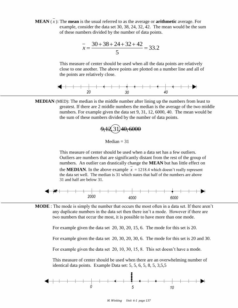
MEAN ( x ): The mean is the usual referred to as the average or arithmetic average. For

example, consider the data set 30, 38, 24, 32, 42. The mean would be the sum

of these numbers divided by the number of data points.

30 38 24 32 4233.2

5x

This measure of center should be used when all the data points are relatively

close to one another. The above points are plotted on a number line and all of

the points are relatively close.

MEDIAN (MED): The median is the middle number after lining up the numbers from least to

greatest. If there are 2 middle numbers the median is the average of the two middle

numbers. For example given the data set 9, 31, 12, 6000, 40. The mean would be

the sum of these numbers divided by the number of data points.

9,12,31,40,6000

Median = 31

This measure of center should be used when a data set has a few outliers.

Outliers are numbers that are significantly distant from the rest of the group of

numbers. An outlier can drastically change the MEAN but has little effect on

the MEDIAN. In the above example x = 1218.4 which doesn’t really represent

the data set well. The median is 31 which states that half of the numbers are above

31 and half are below 31.

MODE : The mode is simply the number that occurs the most often in a data set. If there aren’t

any duplicate numbers in the data set then there isn’t a mode. However if there are

two numbers that occur the most, it is possible to have more than one mode.

For example given the data set 20, 30, 20, 15, 6. The mode for this set is 20.

For example given the data set 20, 30, 20, 30, 6. The mode for this set is 20 and 30.

For example given the data set 20, 10, 30, 15, 8. This set doesn’t have a mode.

This measure of center should be used when there are an overwhelming number of

identical data points. Example Data set: 5, 5, 6, 5, 8, 5, 3,5,5

0 5 10

2000 4000 6000

20 30 40


1. A person is trying to find new employees to work for his company. She wants to

show applicants a statistic about how much her employees make. Which measure

of a center would the best to describe salaries at her company if she knows that 10

of her employees make the following annual salaries?

$11,000 $10,000 $91,000 $92,000 $80,000

$81,000 $88,000 $93,000 $91,000 $73,000

MEAN = MEDIAN = MODE=

Which center measure is most appropriate and why?

2. A company is selling boxes of crackers and wishes to list the number of crackers

that they are contained in a box. A market research found 20 different boxes. Each

box contained the following number of crackers. What number should they list on

the box as the number of crackers in the box mean median or mode?

45 50 48 50 50 50 51 50 50 50

49 50 50 51 50 50 50 54 50 51


Which center measure is most appropriate and why?

3. A student has the following grades in a Math class:

94 92 85 90 96 94 100 92 0 80


Which measure of center do you think should be used to determine the students

grade and why?

4. A student has the following grades in a Math class:

70, 72, 68, 67, 71, 98, 100, 92, 71, 88


Which measure of center do you think should be used to determine the students

grade and why?


5. An employee is working at a clock shop. The clocks on the wall

show the following times:

4:40pm, 4:43pm, 4:43pm, 4:46pm, 4:59pm, 4:43pm, 4:43pm, 4:43pm, 4:55pm, 4:43pm


Which measure of center do you think should be used to determine the correct time

and why?

6. A college wanted to list a meaningful statistic in a brochure showing the ages of

the students attending their college. Below is a random sample of their students:

20, 24, 23, 26, 24, 29, 19, 21, 66, 62, 24, 28, 20, 67, 22, 20, 20, 79, 20, 20


Which measure of center do you think should be used on the brochure and why?

7. A student scored 92, 85, and 87 on their first three tests. What would they need to make on their fourth test to have an ‘A’ test average (90%)?

8. A person at the mall purchased 4 shirts at an average price of $14. How much did the 5th shirt cost if the average after the 5th shirt was purchased changed to $16 per shirt?


9. Consider the data set 5, 2, 8, 14, 11 a. What is the mean of the data set? b. What is the mode of the data set?

c. If 3 were added to each number in the data set, what effect would this have on the mean and the median?

d. If each number in the data set was doubled, what effect would this have on the mean

and the median?


Sec 6.2 - Describing Data Variations (Spread) Name:

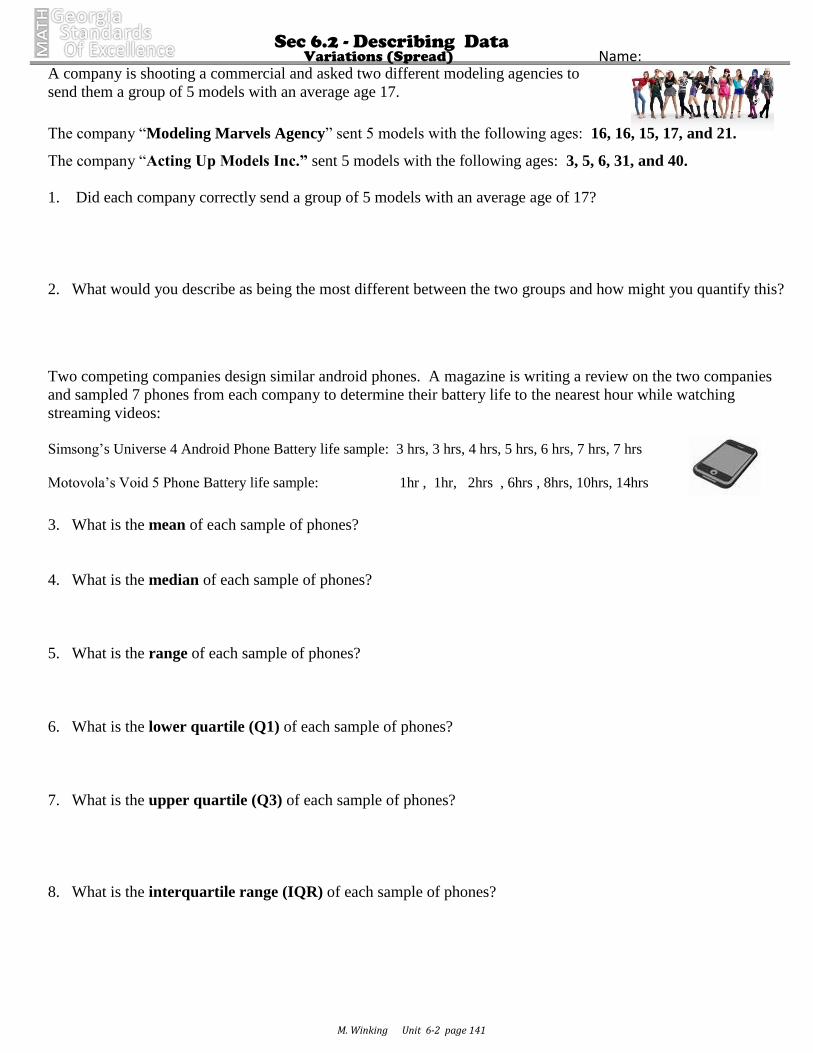
A company is shooting a commercial and asked two different modeling agencies to

send them a group of 5 models with an average age 17.

The company “Modeling Marvels Agency” sent 5 models with the following ages: 16, 16, 15, 17, and 21.

The company “Acting Up Models Inc.” sent 5 models with the following ages: 3, 5, 6, 31, and 40.

1. Did each company correctly send a group of 5 models with an average age of 17?

2. What would you describe as being the most different between the two groups and how might you quantify this?

Two competing companies design similar android phones. A magazine is writing a review on the two companies

and sampled 7 phones from each company to determine their battery life to the nearest hour while watching

streaming videos:

Simsong’s Universe 4 Android Phone Battery life sample: 3 hrs, 3 hrs, 4 hrs, 5 hrs, 6 hrs, 7 hrs, 7 hrs

Motovola’s Void 5 Phone Battery life sample: 1hr , 1hr, 2hrs , 6hrs , 8hrs, 10hrs, 14hrs

3. What is the mean of each sample of phones?

4. What is the median of each sample of phones?

5. What is the range of each sample of phones?

6. What is the lower quartile (Q1) of each sample of phones?

7. What is the upper quartile (Q3) of each sample of phones?

8. What is the interquartile range (IQR) of each sample of phones?


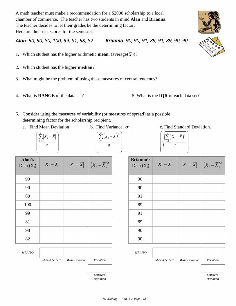
A math teacher must make a recommendation for a $2000 scholarship to a local

chamber of commerce. The teacher has two students in mind Alan and Brianna.

The teacher decides to let their grades be the determining factor.

Here are their test scores for the semester:

Alan: 90, 90, 80, 100, 99, 81, 98, 82 Brianna: 90, 90, 91, 89, 91, 89, 90, 90

1. Which student has the higher arithmetic mean, (average X )?

2. Which student has the higher median?

3. What might be the problem of using these measures of central tendency?

4. What is RANGE of the data set? 5. What is the IQR of each data set?

6. Consider using the measures of variability (or measures of spread) as a possible

determining factor for the scholarship recipient.

a. Find Mean Deviation b. Find Variance, 2 . c. Find Standard Deviation.

n

XXn

i

i

1

n

XXn

i

i

1

2

2

1

n

i

i

X X

n

Alan’s

Data (Xi)

XX i

XX i

2XX i

Brianna’s

Data (Xi)

XX i

XX i

2XX i

90 90

90 90

80 91

100 89

99 91

81 89

98 90

82 90

MEANS:

MEANS:

Should be Zero Mean Deviation Variation Should be Zero Mean Deviation Variation

Standard

Deviation Standard

Deviation


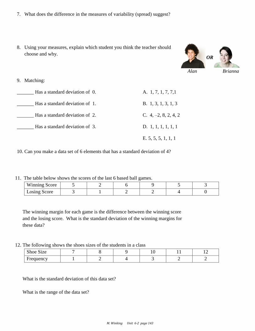
7. What does the difference in the measures of variability (spread) suggest?

8. Using your measures, explain which student you think the teacher should

choose and why.

9. Matching:

Has a standard deviation of 0. A. 1, 7, 1, 7, 7,1

Has a standard deviation of 1. B. 1, 3, 1, 3, 1, 3

Has a standard deviation of 2. C. 4, –2, 8, 2, 4, 2

Has a standard deviation of 3. D. 1, 1, 1, 1, 1, 1

E. 5, 5, 5, 1, 1, 1

10. Can you make a data set of 6 elements that has a standard deviation of 4?

11. The table below shows the scores of the last 6 based ball games.

Winning Score 5 2 6 9 5 3

Losing Score 3 1 2 2 4 0

The winning margin for each game is the difference between the winning score

and the losing score. What is the standard deviation of the winning margins for

these data?

12. The following shows the shoes sizes of the students in a class

Shoe Size 7 8 9 10 11 12

Frequency 1 2 4 3 2 2

What is the standard deviation of this data set?

What is the range of the data set?

Alan Brianna

OR


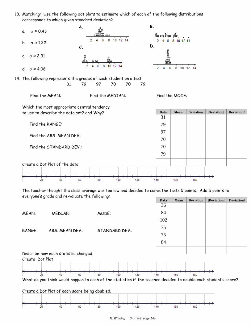
13. Matching: Use the following dot plots to estimate which of each of the following distributions

corresponds to which given standard deviation?

a. ≈ 0.43

b. ≈ 1.22

c. ≈ 2.91

d. ≈ 4.08

14. The following represents the grades of each student on a test

31 79 97 70 70 79

Find the MEAN: Find the MEDIAN: Find the MODE:

Which the most appropriate central tendency

to use to describe the data set? and Why?

Find the RANGE:

Find the ABS. MEAN DEV.:

Find the STANDARD DEV.:

Create a Dot Plot of the data:

The teacher thought the class average was too low and decided to curve the tests 5 points. Add 5 points to

everyone’s grade and re-valuate the following:

MEAN: MEDIAN: MODE:

RANGE: ABS. MEAN DEV.: STANDARD DEV.:

Describe how each statistic changed.

Create Dot Plot

What do you think would happen to each of the statistics if the teacher decided to double each student’s score?

Create a Dot Plot of each score being doubled.

A. B.

C. D.

Data Mean Deviation |Deviation| Deviation2

31

79

97

70

70

79

Data Mean Deviation |Deviation| Deviation2

36

84

102

75

75

84


Sec 6.3 - Describing Data Data Graphs Name:

1. Create a Basic Box and Whisker Plot of the following data sets: a. 3, 4, 4, 8, 9, 12, 15

b. 2, 9, 3, 14, 3, 2, 3

c. 5, 9, 14, 12, 10, 3, 15, 5, 8, 7

2. Determine the suggested statistical measures and answer the questions based on the graph.

a. Minimum =

b. Q3 =

c. IQR =

d. Range=

e. Which quartile has the most variation?


a. Minimum =

b. Q1 =

c. IQR =

d. Median=

e. Which quartile has the most variation?


a. Minimum =

b. Maximum =

c. Outliers =

d. Median=

5. Given the data set , 5, 80, 75, 62, 64, 90, 75, 94, 100, determine which if any of the data points are outliers by definition ( or ) and create an Advanced Box and Whisker plot.


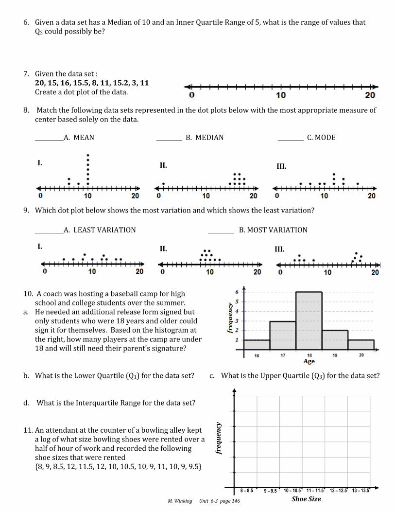
6. Given a data set has a Median of 10 and an Inner Quartile Range of 5, what is the range of values that Q3 could possibly be?

7. Given the data set : 20, 15, 16, 15.5, 8, 11, 15.2, 3, 11 Create a dot plot of the data.

8. Match the following data sets represented in the dot plots below with the most appropriate measure of

center based solely on the data. __________A. MEAN _________ B. MEDIAN _________ C. MODE

9. Which dot plot below shows the most variation and which shows the least variation?

__________A. LEAST VARIATION _________ B. MOST VARIATION

10. A coach was hosting a baseball camp for high

school and college students over the summer. a. He needed an additional release form signed but

only students who were 18 years and older could sign it for themselves. Based on the histogram at the right, how many players at the camp are under 18 and will still need their parent’s signature?

b. What is the Lower Quartile (Q1) for the data set?

c. What is the Upper Quartile (Q3) for the data set?

d. What is the Interquartile Range for the data set?

11. An attendant at the counter of a bowling alley kept a log of what size bowling shoes were rented over a half of hour of work and recorded the following shoe sizes that were rented {8, 9, 8.5, 12, 11.5, 12, 10, 10.5, 10, 9, 11, 10, 9, 9.5}

I. II. III.

I. II. III.

Shoe Size

freq

ue

ncy

10 – 10.5 11 – 11.5 12 – 12.5 13 – 13.5 9 – 9.5 8 – 8.5


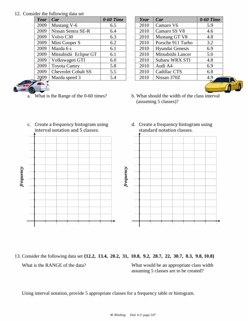
12. Consider the following data set

Year Car 0-60 Time Year Car 0-60 Time

2009 Mustang V-6 6.5 2010 Camaro V6 5.9

2009 Nissan Sentra SE-R 6.4 2010 Camaro SS V8 4.6

2009 Volvo C30 6.3 2010 Mustang GT V8 4.8

2009 Mini Cooper S 6.2 2010 Porsche 911 Turbo 3.2

2009 Mazda 6 s 6.1 2010 Hyundai Genesis 6.9

2009 Mitsubishi Eclipse GT 6.1 2010 Mitsubishi Lancer 5.0

2009 Volkswagen GTI 6.0 2010 Subaru WRX STI 4.8

2009 Toyota Camry 5.8 2010 Audi A4 6.9

2009 Chevrolet Cobalt SS 5.5 2010 Cadillac CTS 6.8

2009 Mazda speed 3 5.4 2010 Nissan 370Z 4.9

a. What is the Range of the 0-60 times? b. What should the width of the class interval

(assuming 5 classes)?

c. Create a frequency histogram using

interval notation and 5 classes.

d. Create a frequency histogram using standard notation classes.

13. Consider the following data set {12.2, 13.4, 20.2, 31, 10.8, 9.2, 28.7, 22, 30.7, 8.3, 9.8, 10.8}

What is the RANGE of the data? What would be an appropriate class width

assuming 5 classes are to be created?

Using interval notation, provide 5 appropriate classes for a frequency table or histogram.

freq

ue

ncy

freq

ue

ncy


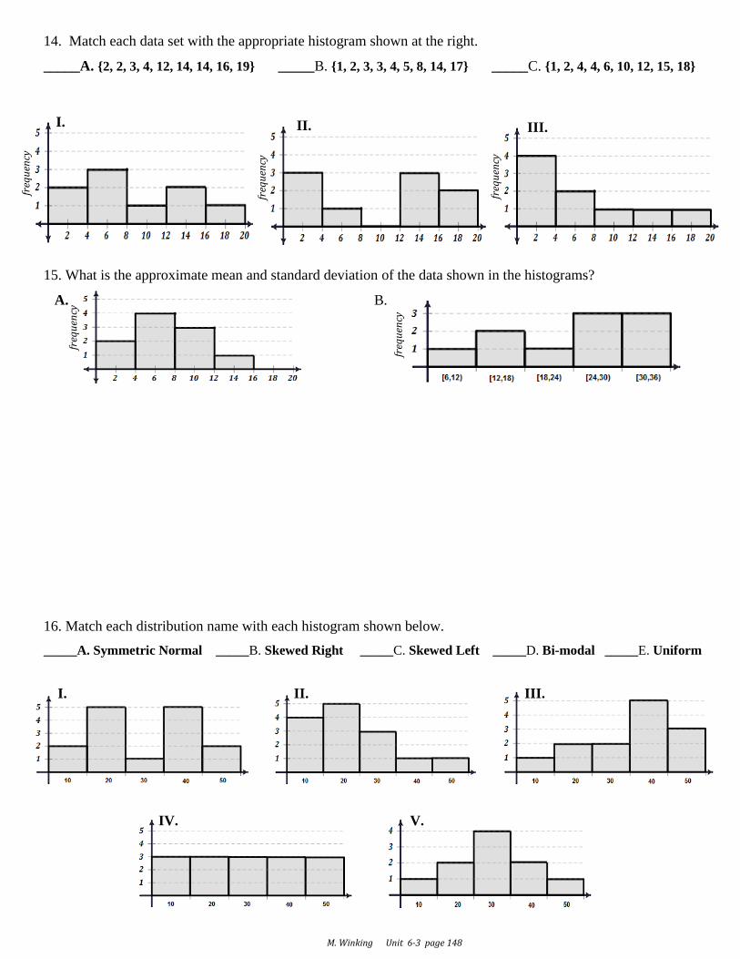
14. Match each data set with the appropriate histogram shown at the right.

_____A. {2, 2, 3, 4, 12, 14, 14, 16, 19} _____B. {1, 2, 3, 3, 4, 5, 8, 14, 17} _____C. {1, 2, 4, 4, 6, 10, 12, 15, 18}

15. What is the approximate mean and standard deviation of the data shown in the histograms?

A. B.

16. Match each distribution name with each histogram shown below.

_____A. Symmetric Normal _____B. Skewed Right _____C. Skewed Left _____D. Bi-modal _____E. Uniform

I. II. III.

freq

uen

cy

freq

uen

cy

freq

uen

cy

freq

uen

cy

freq

uen

cy

I. II. III.

IV. V.


JAWS 2: Incident at Arched Rock By Dave Cone

Originally published in Bay Currents, Nov 1993

This time we can joke about it-nobody got hurt. For the second year in a row,

autumn in Northern California was marked by a Great White Shark attack on a

coastal kayaker.

Rosemary Johnson is a lifelong ocean sports enthusiast now living in

Sonoma County. On Sunday October 10, she and three companions set off

from Goat Rock Beach south of Jenner for the short paddle southward to

Arched Rock (another Arch Rock lies north of Jenner). Rosemary was

paddling a borrowed blue Frenzy, which is a plastic sit-on-top boat just

nine feet long. Her friend Rick Larson, on his second kayak trip ever, was

on a Scupper, and one of the others paddled a Kiwi, which is also a very

short kayak.

As the four paddlers approached Arched Rock, Rosemary veered off from the group and headed around the rock.

Rick and the others soon followed at some distance. Rosemary felt a powerful jolt and flew off the top of her boat.

Rick saw a shark perhaps 16 feet long knock the boat entirely out of the water, and he believes Rosemary

flew 12 to 14 feet into the air. Rosemary landed in the water, and briefly felt something solid

underfoot. She thinks she landed on the shark. Wearing a wetsuit but no life vest, she had to swim in one direction to

nab her paddle, then back the other way to get to her boat. She remained calm, believing that she had merely struck a

rock. Her approaching companions were less than calm, having seen the "monster" that hit her boat. Rick states that

the shark's mouth encompassed almost the whole width of the Frenzy.

Rosemary hopped back on her kayak, but immediately capsized. She re-entered a second time and attempted to head

toward shore, but had difficulty controlling the boat. When she capsized again, her friends saw the bite marks on her

hull and realized that her boat was tippy and unmanageable because it was taking on water. They quickly improvised

a rescue, with Rosemary riding belly down and head aft on the front of Rick's Scupper-"the only boat that could take

me"-and the other paddlers towing the punctured boat. The group returned to the beach without further difficulty.

Back on dry land, the party reported the incident to Sonoma State Beaches rangers and inspected the boat. The

damage measures 20 by 15 inches and lies entirely below the waterline approximately beneath the seat. A jagged

crack runs perpendicular to the line of tooth marks. The pattern differs from the evidence left on Ken Kelton's boat,

which shows tooth marks on both deck and hull (see "Ano Nuevo Revisited," Bay Currents, Dec. '92). Ken's shark

held his boat for five to ten seconds, while Rosemary's contact was a collision rather than a grab-and-shake. Although

it's common for sharks to intentionally release their prey after the initial attack, it is also possible that this shark

simply bit more than it could chew, and Rosemary's boat popped out of its jaw like a watermelon seed between your

fingers.

A researcher at Bodega Bay Marine Lab told the state park folks the size of the bite marks is consistent with a Great White up to 14 feet and 1500 pounds. Photos of the bite mark have been sent to shark expert Dr.

Mark Marks at Humboldt State for more detailed analysis.

Park Rangers posted the beaches from Russian River to Bodega Head with

shark warnings for five days after the attack, on the reasoning that Great Whites

typically feed in an area for a few days and then move on. Of the numerous

press accounts of the attack, the silliest was in the Santa Rosa Press-Democrat,

which stated that "(Head Ranger Brian) Hickey said rangers don't know if the

shark attacked on the first or last day it was in the Goat Rock area." Evidently

the reporter was surprised that Hickey didn't have a copy of the shark's MISTIX

reservation.

Rosemary and Rick visited the October 27 BASK general meeting, where

Rosemary was peppered with questions, a few of them pertinent, and awarded a

shark tee shirt and refrigerator magnet. Ken Kelton, BASK's own poster child

for shark survival, greeted Rosemary, saying "You and I are members of a very

exclusive club." Most of us are happy to see that club remain small.

How are such PREDICTIONS made?


HINT: Use your Trend Line

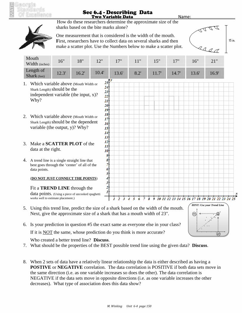
Sec 6.4 - Describing Data Two Variable Data Name:

How do these researchers determine the approximate size of the

sharks based on the bite marks alone?

One measurement that is considered is the width of the mouth.

First, researchers have to collect data on several sharks and then

make a scatter plot. Use the Numbers below to make a scatter plot.

Mouth

Width (inches) 16" 18" 12" 17" 11" 15" 17" 16" 21"

Length of

Shark (feet) 12.3' 16.2'

10.4' 13.6' 8.2' 11.7' 14.7' 13.6' 16.9'

1. Which variable above (Mouth Width or

Shark Length) should be the

independent variable (the input, x)?

Why?

2. Which variable above (Mouth Width or

Shark Length) should be the dependent

variable (the output, y)? Why?

3. Make a SCATTER PLOT of the

data at the right.

4. A trend line is a single straight line that

best goes through the ‘center’ of all of the

data points.

(DO NOT JUST CONNECT THE POINTS)

Fit a TREND LINE through the

data points. (Using a piece of uncooked spaghetti

works well to estimate placement.)

5. Using this trend line, predict the size of a shark based on the width of the mouth.

Next, give the approximate size of a shark that has a mouth width of 23".

6. Is your prediction in question #5 the exact same as everyone else in your class?

If it is NOT the same, whose prediction do you think is more accurate?

Who created a better trend line? Discuss.

7. What should be the properties of the BEST possible trend line using the given data? Discuss.

8. When 2 sets of data have a relatively linear relationship the data is either described as having a

POSTIVE or NEGATIVE correlation. The data correlation is POSITIVE if both data sets move in

the same direction (i.e. as one variable increases so does the other). The data correlation is

NEGATIVE if the data sets move in opposite directions (i.e. as one variable increases the other

decreases). What type of association does this data show?

23”

??


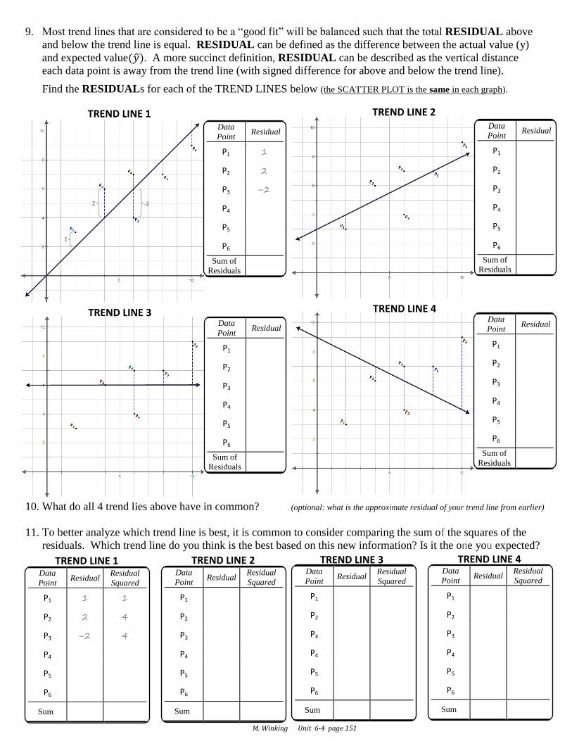
9. Most trend lines that are considered to be a “good fit” will be balanced such that the total RESIDUAL above

and below the trend line is equal. RESIDUAL can be defined as the difference between the actual value (y)

and expected value . A more succinct definition, RESIDUAL can be described as the vertical distance

each data point is away from the trend line (with signed difference for above and below the trend line).

Find the RESIDUALs for each of the TREND LINES below (the SCATTER PLOT is the same in each graph).

10. What do all 4 trend lies above have in common? (optional: what is the approximate residual of your trend line from earlier)

11. To better analyze which trend line is best, it is common to consider comparing the sum of the squares of the

residuals. Which trend line do you think is the best based on this new information? Is it the one you expected?

Data

Point Residual

P1 1

P2 2

P3 –2

P4

P5

P6

Sum of

Residuals

Data

Point Residual

P1

P2

P3

P4

P5

P6

Sum of

Residuals

Data

Point Residual

P1

P2

P3

P4

P5

P6

Sum of

Residuals

Data

Point Residual

P1

P2

P3

P4

P5

P6

Sum of

Residuals

TREND LINE 1 TREND LINE 2

TREND LINE 3 TREND LINE 4

-2

1

2

Data

Point Residual

Residual

Squared

P1 1 1

P2 2 4

P3 –2 4

P4

P5

P6

Sum

Data

Point Residual

Residual

Squared

P1

P2

P3

P4

P5

P6

Sum

Data

Point Residual

Residual

Squared

P1

P2

P3

P4

P5

P6

Sum

Data

Point Residual

Residual

Squared

P1

P2

P3

P4

P5

P6

Sum

TREND LINE 1 TREND LINE 2 TREND LINE 3 TREND LINE 4


12. The line that minimizes the squares is called the LEAST SQUARES REGRESSION LINE. Most scientific

calculators are capable of determining the equation of this trend line. Consider again the data about sharks.

The following are the directions for the TI-83/84:

1) First, it will be helpful to turn on additional diagnostic information in your calculator.

…….…

2) Under the Stat menu, press . (This just resets the list menus)

3) Next, press

4) If there is OLD data already in the lists that needs to be cleared press the

up arrow, , to highlight L1 and then press to clear out

the old data. Do the same for L2 if it has OLD data that needs to be

cleared.

5) Next, enter the Shark’s Mouth Size in L1 and the Length of the Shark in L2.

6) Return to the home screen by pressing and then to calculate the

linear regression press .

7) This represents the an equation of a line that minimizes the total residuals squared.

Fill in the blanks to complete the LEAST SQUARES REGRESSION LINE equation.

y = x +

Use this equation to reattempt your prediction of a shark with a 23” mouth.

y = (23) + =

Now, was this close to your original prediction?

13. When a prediction is made between two given data points the prediction is called an INTERPOLATION.

When a prediction is made outside the range of given data points the prediction is an EXTRAPOLATION.

Which type of prediction was used when you predicted the length of a shark with a 23” wide mouth?

14. In the movie JAWS the shark was approximately 35 feet in

length, based on the equation you just calculated, how wide

would his mouth be? (careful the length might be represented by x)

Would it be large enough to bite the back end of a boat

(consider even a small boat is 48 inches wide)?

CATALOG SCROLL DOWN TO DianosticOn

To clear out OLD data, first highlight

L1 and press

CLEAR, ENTER.

a b

a b

35 = x + a b


15. A calculation called the correlation coefficient (r) is used to measure the extent to which the data for the

two variables show a linear relationship. The closer the value is to 1 or –1 the stronger the linear

relationship.

16. Match the correct Correlation Coefficient with the correct scatter plot:

r ≈ 0. 98

r ≈ – 0. 96

r ≈ 0.61

r ≈ 0.17

17. Create a scatter plot and approximate a trend line of best fit based on the data below

a.

b. Using your calculator determine the approximate linear regression line that best fits the data.

c. Use your model, to predict the 0-60mph time of a car that costs $30 K?

d. Was your prediction in problem (part c) an extrapolation or

interpolation?

e. Use your model, to predict how much a car would cost that can do 0 – 60 mph in 4.0 seconds.

(Show Work!)

0

Perfect Positive Linear

Relationship

No Linear

Relationship

Perfect Negative

Linear

Relationship

Strong Weak None Strong Weak

r:

Model Cost of

Car 0-60 mph

acceleration Scion xB $16 K 7.8 sec

Mitsubishi Eclipse $24 K 6.1 sec

Chev. Corvette $106 K 3.4 sec

Nissan GT-R $76 K 3.5 sec

SSC Ultimate Aero $42 K 4.8 sec

Lotus Elise $60 K 4.4 sec

Honda Civic Si $22 K 6.7 sec

y = .x + (a) (b)

3c.

Extrapolation Interpolation

3d.

3e .

a.

A. B. C. D.


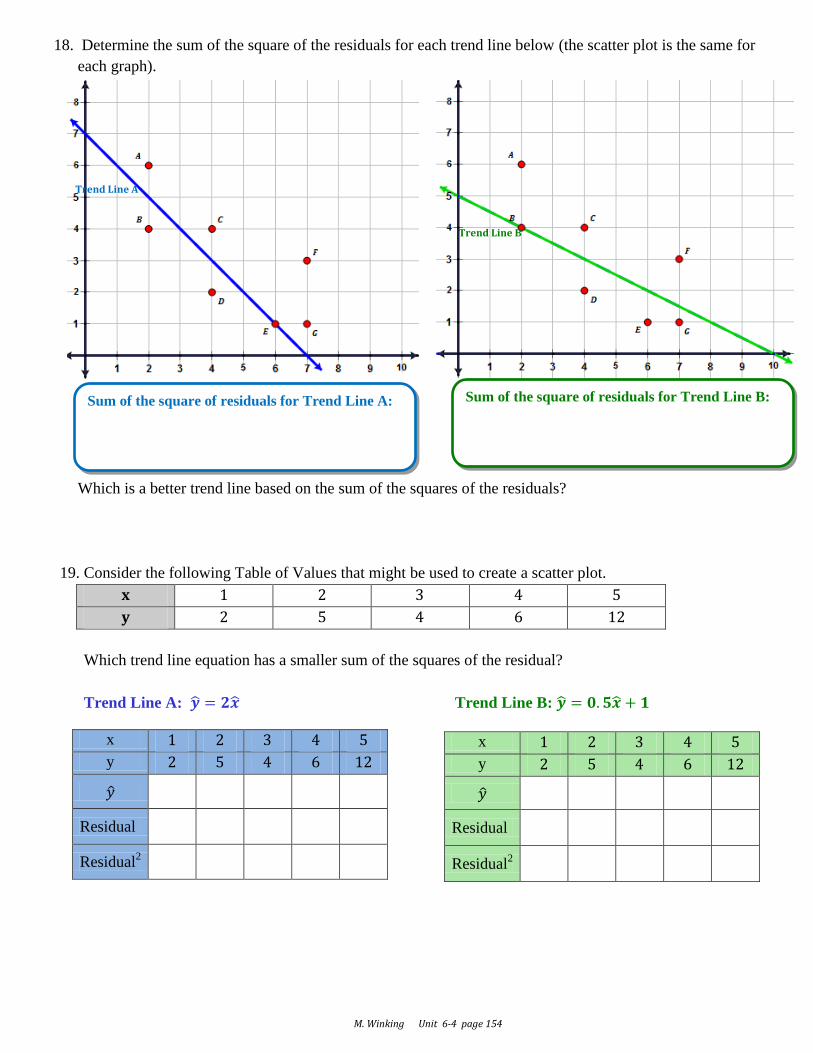
18. Determine the sum of the square of the residuals for each trend line below (the scatter plot is the same for

each graph).

Which is a better trend line based on the sum of the squares of the residuals?

19. Consider the following Table of Values that might be used to create a scatter plot.

x 1 2 3 4 5

y 2 5 4 6 12

Which trend line equation has a smaller sum of the squares of the residual?

Trend Line A: Trend Line B:

Trend Line A

Trend Line B

Sum of the square of residuals for Trend Line A:

Sum of the square of residuals for Trend Line B:

x 1 2 3 4 5

y 2 5 4 6 12

Residual

Residual2

x 1 2 3 4 5

y 2 5 4 6 12

Residual

Residual2


Sec 6.1 N Central Tendencies - Gwinnett County Public …€¦ · · 2017-04-10N Central...

Documents

Transcript of Sec 6.1 N Central Tendencies - Gwinnett County Public …€¦ · · 2017-04-10N Central...