Seasonal weather forecasting:- the motivations- the capabilities

- the atmospheric physics involved

J.D. McAlpine

ATMS 611, autumn 2010

Class project

photo credit: Michelle Meiklejohn /freedigitalphotos.netphoto credit: pixomar /freedigitalphotos.net

photo credit: J.D. McAlpine Graphic from www.cpc.noaa.gov

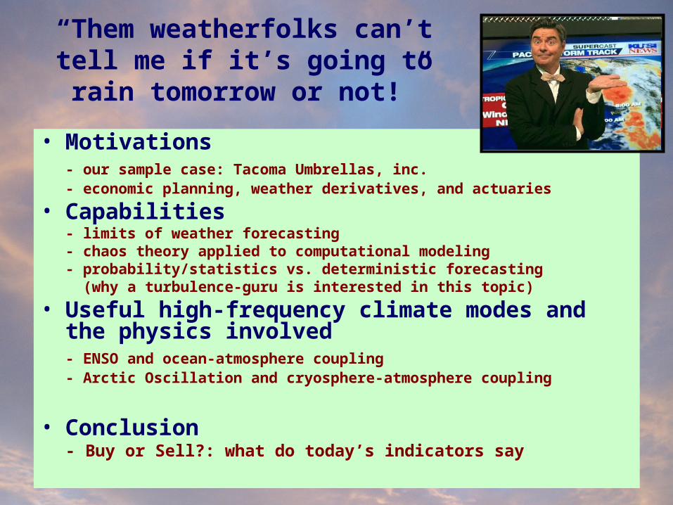
“Them weatherfolks can’t tell me if it’s going to rain tomorrow or not!”

• Motivations- our sample case: Tacoma Umbrellas, inc.- economic planning, weather derivatives, and actuaries

• Capabilities- limits of weather forecasting- chaos theory applied to computational modeling- probability/statistics vs. deterministic forecasting (why a turbulence-guru is interested in this topic)

• Useful high-frequency climate modes and the physics involved

- ENSO and ocean-atmosphere coupling- Arctic Oscillation and cryosphere-atmosphere coupling

• Conclusion- Buy or Sell?: what do today’s indicators say

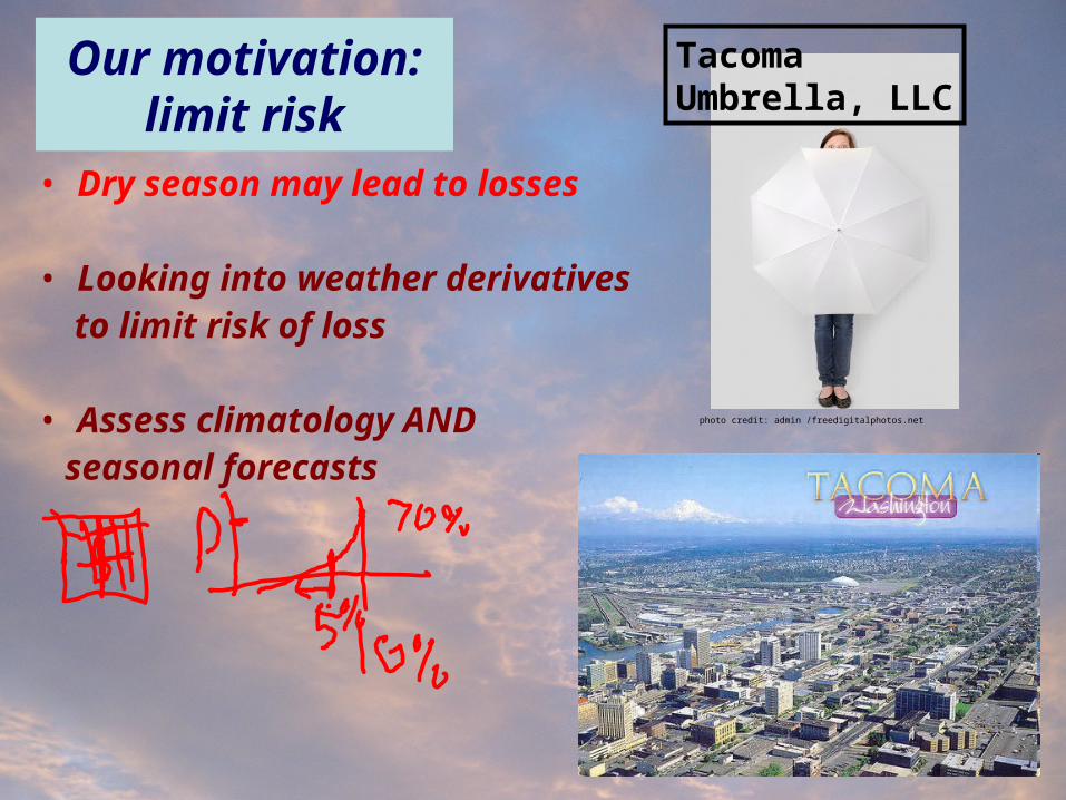
Our motivation: limit risk

• Dry season may lead to losses

• Looking into weather derivatives to limit risk of loss

• Assess climatology AND seasonal forecasts

Tacoma Umbrella, LLC

photo credit: admin /freedigitalphotos.net

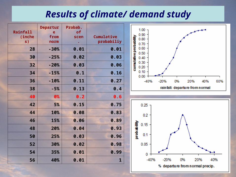
Results of climate/ demand study

Rainfall (inches)

Departure from norm

Probab. of scen.

Cumulative probabiliy

28 -30% 0.01 0.01

30 -25% 0.02 0.03

32 -20% 0.03 0.06

34 -15% 0.1 0.16

36 -10% 0.11 0.27

38 -5% 0.13 0.4

40 0% 0.2 0.6

42 5% 0.15 0.75

44 10% 0.08 0.83

46 15% 0.06 0.89

48 20% 0.04 0.93

50 25% 0.03 0.96

52 30% 0.02 0.98

54 35% 0.01 0.99

56 40% 0.01 1

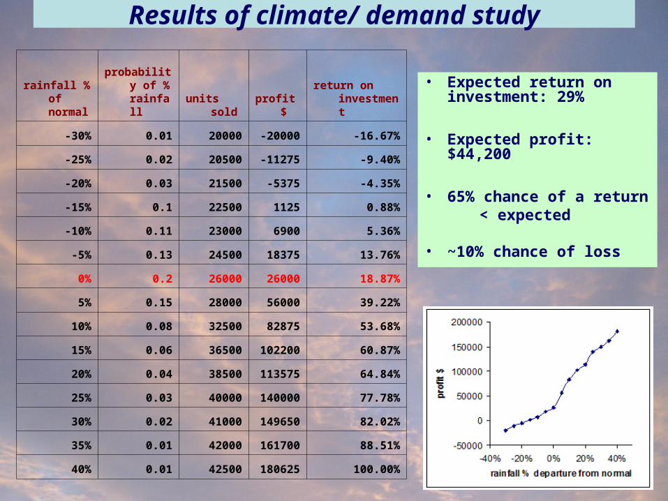
Results of climate/ demand study

rainfall % of normal

probability of % rainfall units sold profit $

return on investment

-30% 0.01 20000 -20000 -16.67%

-25% 0.02 20500 -11275 -9.40%

-20% 0.03 21500 -5375 -4.35%

-15% 0.1 22500 1125 0.88%

-10% 0.11 23000 6900 5.36%

-5% 0.13 24500 18375 13.76%

0% 0.2 26000 26000 18.87%

5% 0.15 28000 56000 39.22%

10% 0.08 32500 82875 53.68%

15% 0.06 36500 102200 60.87%

20% 0.04 38500 113575 64.84%

25% 0.03 40000 140000 77.78%

30% 0.02 41000 149650 82.02%

35% 0.01 42000 161700 88.51%

40% 0.01 42500 180625 100.00%

• Expected return on investment: 29%

• Expected profit: $44,200

• 65% chance of a return < expected

• ~10% chance of loss

Payoff function:

Where L$=D(K-L), the maximum payout

D is the “tick”: the amount of money per unit = $/(% precip below normal) example: $2500/1%

K is the “strike”: the threshold value of payout = 3.5% above normal

X is the actual value that occurs = ? Look at climate indicators to guess what % of precip

we can expect this year

Weather derivative: Linear put-option purchase

Kxif

KxLifxKD

LxifL

xp

0

)(

$

)(

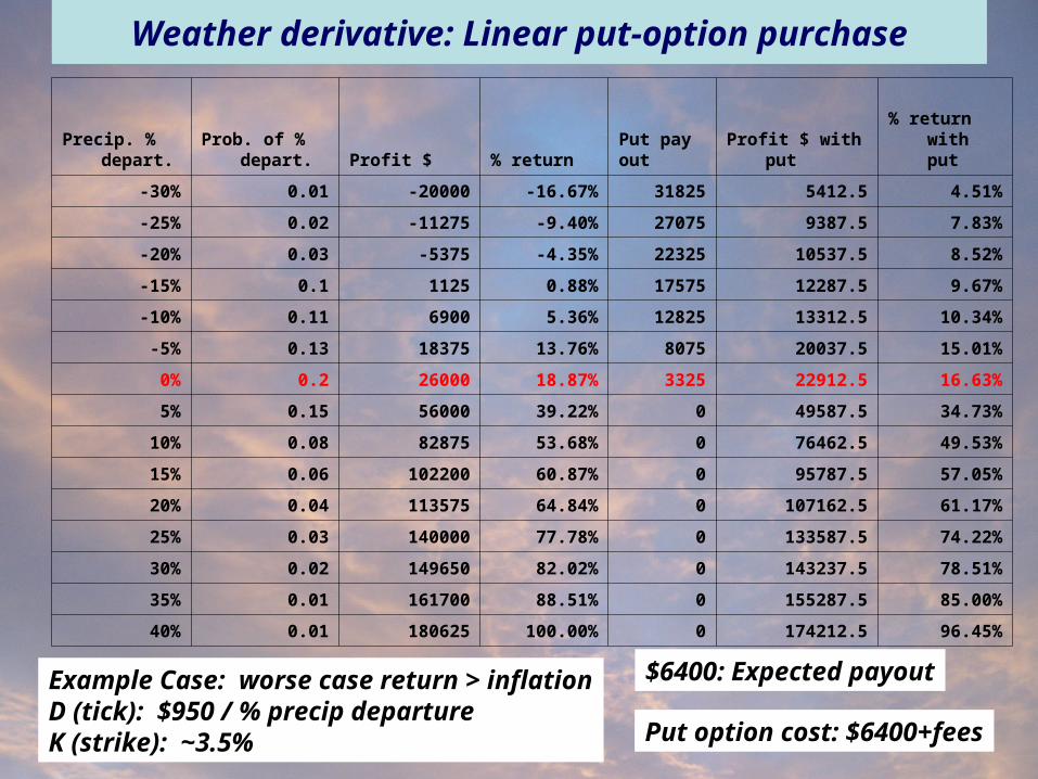
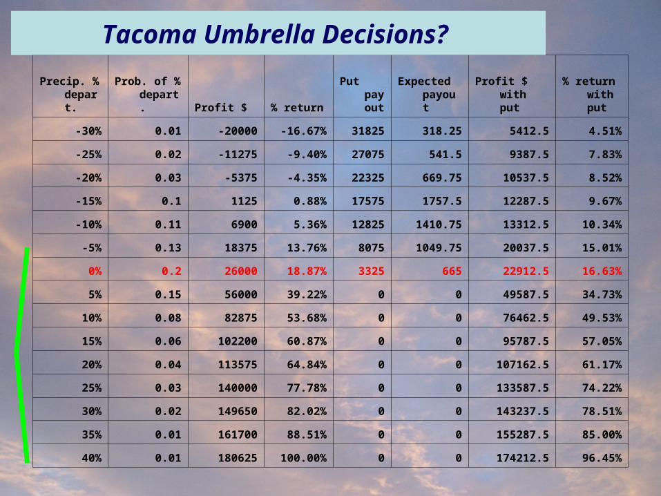
Weather derivative: Linear put-option purchase

Precip. % depart.

Prob. of % depart. Profit $ % return

Put payout Profit $ with put

% return with put

-30% 0.01 -20000 -16.67% 31825 5412.5 4.51%

-25% 0.02 -11275 -9.40% 27075 9387.5 7.83%

-20% 0.03 -5375 -4.35% 22325 10537.5 8.52%

-15% 0.1 1125 0.88% 17575 12287.5 9.67%

-10% 0.11 6900 5.36% 12825 13312.5 10.34%

-5% 0.13 18375 13.76% 8075 20037.5 15.01%

0% 0.2 26000 18.87% 3325 22912.5 16.63%

5% 0.15 56000 39.22% 0 49587.5 34.73%

10% 0.08 82875 53.68% 0 76462.5 49.53%

15% 0.06 102200 60.87% 0 95787.5 57.05%

20% 0.04 113575 64.84% 0 107162.5 61.17%

25% 0.03 140000 77.78% 0 133587.5 74.22%

30% 0.02 149650 82.02% 0 143237.5 78.51%

35% 0.01 161700 88.51% 0 155287.5 85.00%

40% 0.01 180625 100.00% 0 174212.5 96.45%

$6400: Expected payout

Put option cost: $6400+fees

Example Case: worse case return > inflationD (tick): $950 / % precip departureK (strike): ~3.5%

Weather derivative: Linear put-option purchase

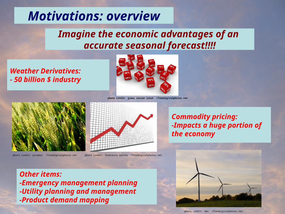
Motivations: overviewImagine the economic advantages of an

accurate seasonal forecast!!!!

Weather Derivatives:- 50 billion $ industry

Commodity pricing:-Impacts a huge portion of the economy

Other items:-Emergency management planning-Utility planning and management-Product demand mapping

photo credit: graur razvan ionut /freedigitalphotos.net

photo credit: francesco marino /freedigitalphotos.net

photo credit: dan /freedigitalphotos.net

photo credit: graur razvan ionut /freedigitalphotos.net

photo credit: pixomar /freedigitalphotos.net

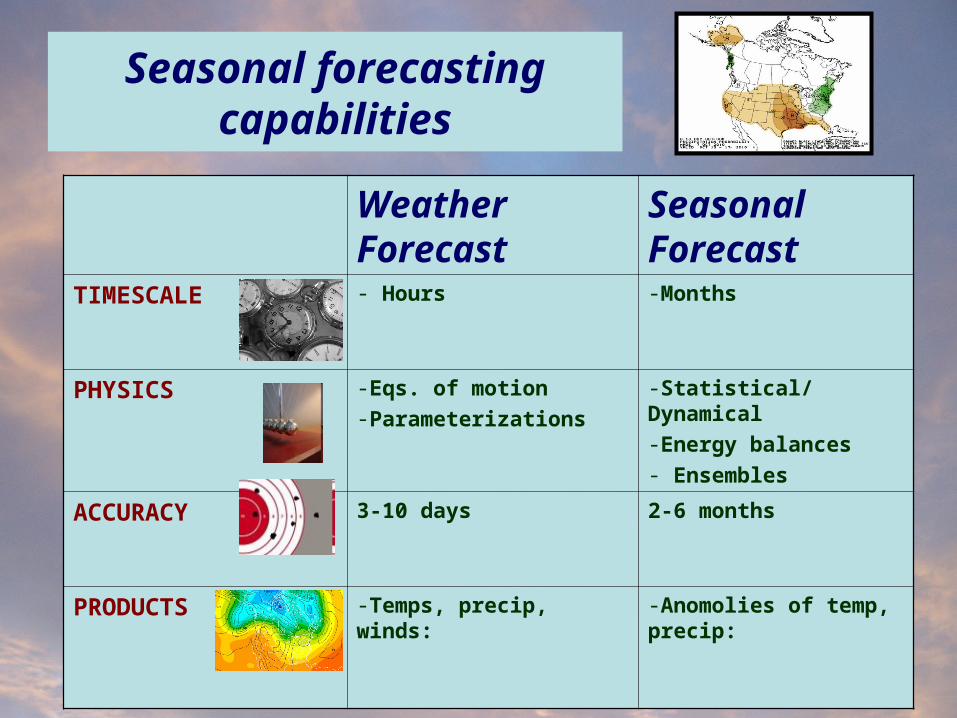
Seasonal forecasting capabilities

Weather Forecast

Seasonal Forecast

TIMESCALE - Hours -Months

PHYSICS -Eqs. of motion-Parameterizations

-Statistical/ Dynamical-Energy balances- Ensembles

ACCURACY 3-10 days 2-6 months

PRODUCTS -Temps, precip, winds:

-Anomolies of temp, precip:

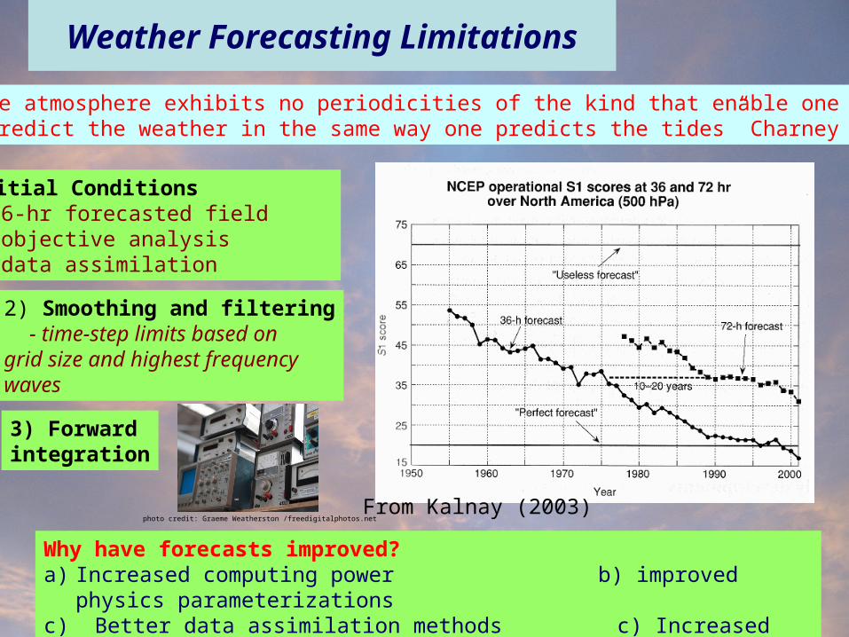
Weather Forecasting Limitations

2) Smoothing and filtering - time-step limits based ongrid size and highest frequencywaves

“ the atmosphere exhibits no periodicities of the kind that enable oneto predict the weather in the same way one predicts the tides” Charney (1951)

1) Initial Conditions a) 6-hr forecasted field b) objective analysis c) data assimilation

Why have forecasts improved?a) Increased computing power b) improved physics parameterizationsc) Better data assimilation methods c) Increased data volume and accuracy

3) Forward integration

Weather Forecasting Limitations

From Kalnay (2003)photo credit: Graeme Weatherston /freedigitalphotos.net

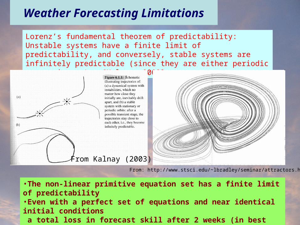
Weather Forecasting Limitations

Lorenz’s fundamental theorem of predictability: Unstable systems have a finite limit of predictability, and conversely, stable systems are infinitely predictable (since they are either periodic or stationary) [Kalnay, 2003]

From Kalnay (2003)From: http://www.stsci.edu/~lbradley/seminar/attractors.html

•The non-linear primitive equation set has a finite limit of predictability•Even with a perfect set of equations and near identical initial conditions a total loss in forecast skill after 2 weeks (in best case)

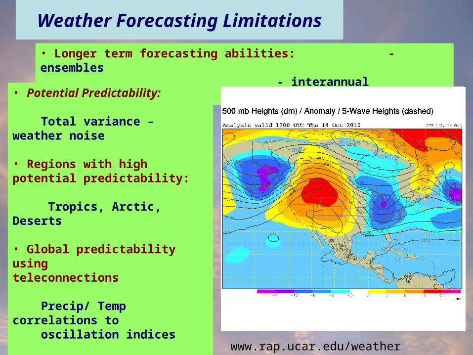
Weather Forecasting Limitations

• Longer term forecasting abilities: - ensembles- interannual predictability

• Potential Predictability:

Total variance – weather noise

• Regions with high potential predictability:

Tropics, Arctic, Deserts

• Global predictability usingteleconnections

Precip/ Temp correlations to oscillation indices

• Major oscillations: ENSO and AO

Weather Forecasting Limitations

www.rap.ucar.edu/weather

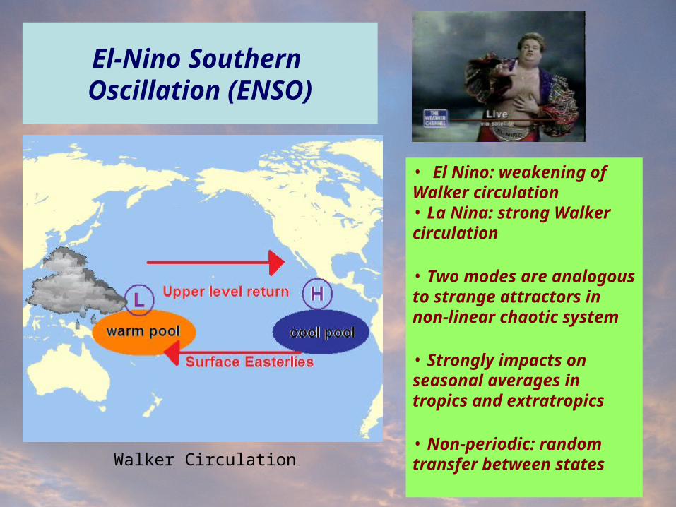
El-Nino Southern Oscillation (ENSO)

• El Nino: weakening of Walker circulation• La Nina: strong Walker circulation

• Two modes are analogous to strange attractors in non-linear chaotic system

• Strongly impacts on seasonal averages in tropics and extratropics

• Non-periodic: random transfer between states

Walker Circulation

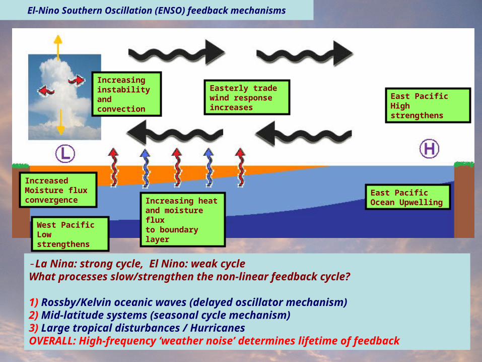
El-Nino Southern Oscillation (ENSO) feedback mechanisms

Easterly trade wind responseincreases

West Pacific Low strengthens

East Pacific Ocean UpwellingIncreasing heat

and moisture fluxto boundary layer

East Pacific High strengthens

-La Nina: strong cycle, El Nino: weak cycleWhat processes slow/strengthen the non-linear feedback cycle?

1) Rossby/Kelvin oceanic waves (delayed oscillator mechanism)2) Mid-latitude systems (seasonal cycle mechanism) 3) Large tropical disturbances / Hurricanes OVERALL: High-frequency ‘weather noise’ determines lifetime of feedback

Increasing instability andconvection

IncreasedMoisture fluxconvergence

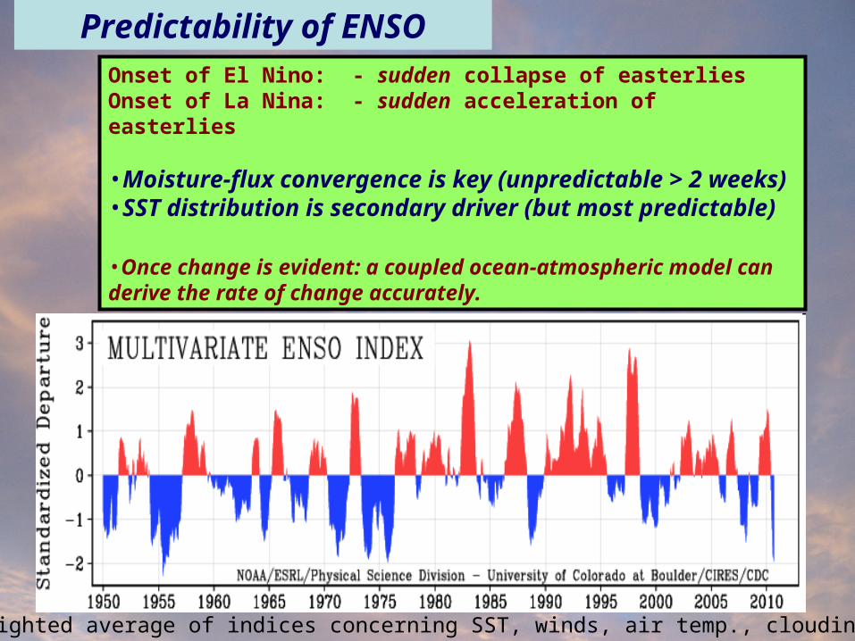
Predictability of ENSOOnset of El Nino: - sudden collapse of easterliesOnset of La Nina: - sudden acceleration of easterlies

•Moisture-flux convergence is key (unpredictable > 2 weeks)•SST distribution is secondary driver (but most predictable)

•Once change is evident: a coupled ocean-atmospheric model can derive the rate of change accurately.

MEI: weighted average of indices concerning SST, winds, air temp., cloudiness

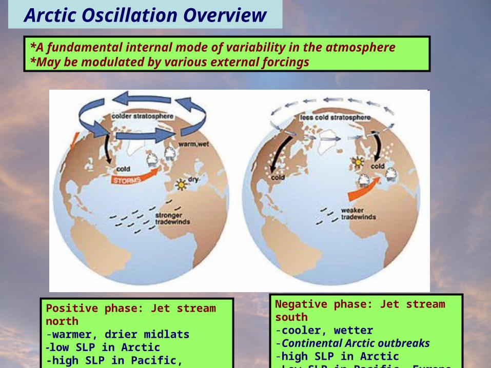
Arctic Oscillation Overview

Positive phase: Jet stream north-warmer, drier midlats-low SLP in Arctic-high SLP in Pacific, Europe

*A fundamental internal mode of variability in the atmosphere*May be modulated by various external forcings

Negative phase: Jet stream south-cooler, wetter-Continental Arctic outbreaks-high SLP in Arctic-Low SLP in Pacific, Europe

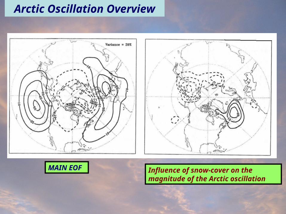
Arctic Oscillation Overview

Influence of snow-cover on the magnitude of the Arctic oscillation

MAIN EOF

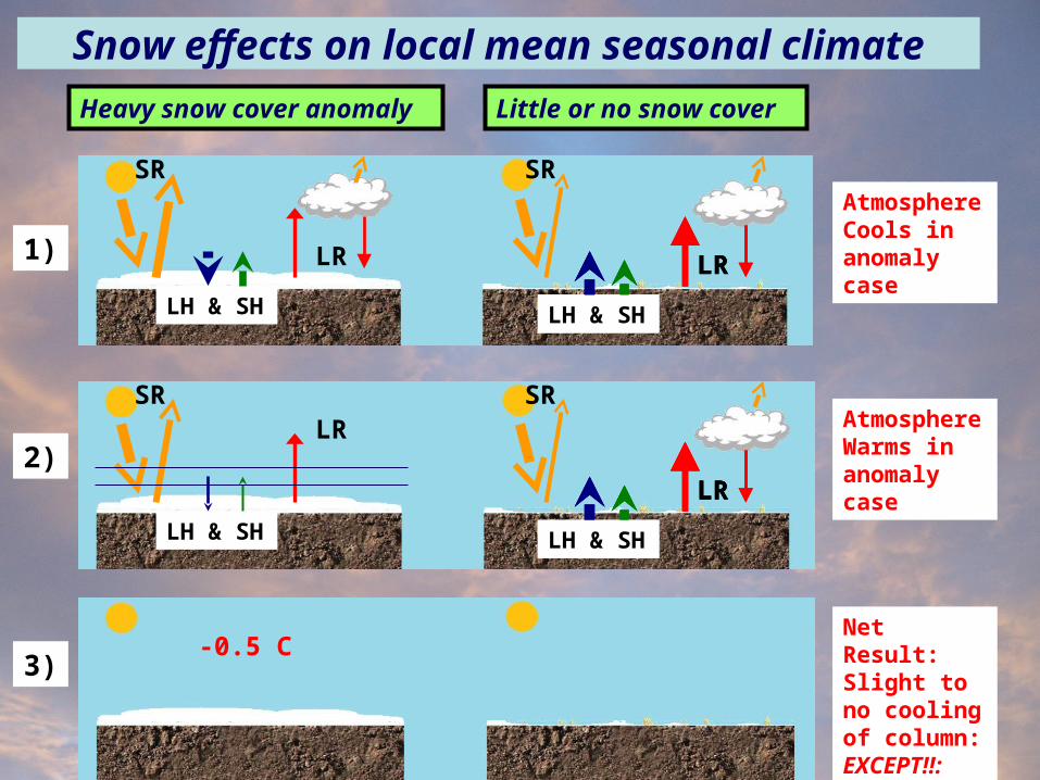
Snow effects on local mean seasonal climate

Heavy snow cover anomaly Little or no snow cover

1)

LH & SH

LR

SR SR

LRLRLR

LH & SHLH & SH

AtmosphereCools in anomaly case

2)

AtmosphereWarms in anomaly case

LH & SH

LR

SR SR

LRLR

LR

LH & SHLH & SH

3)

Net Result:Slight to no cooling of column:EXCEPT!!:

-0.5 C

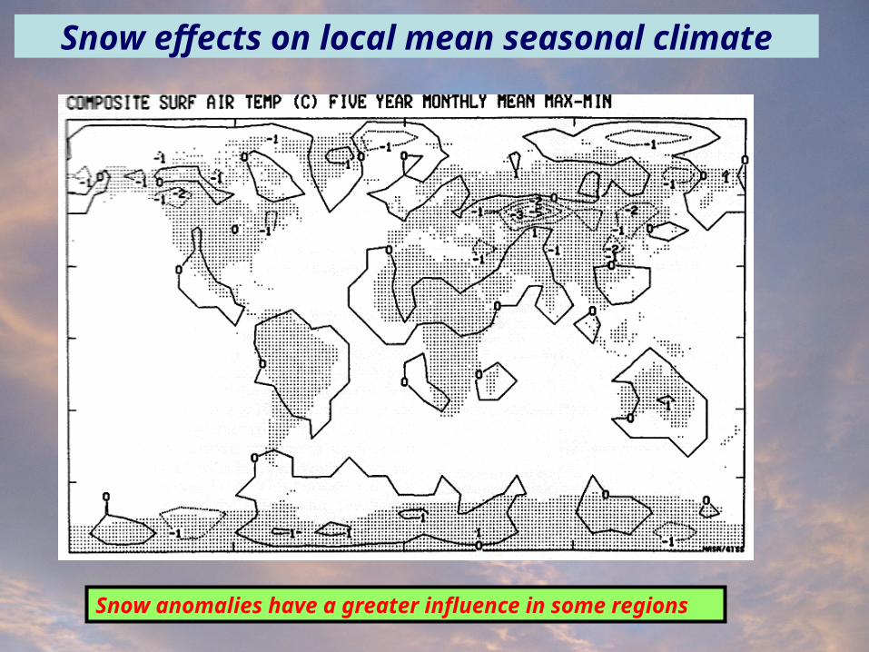
Snow anomalies have a greater influence in some regions

Snow effects on local mean seasonal climate

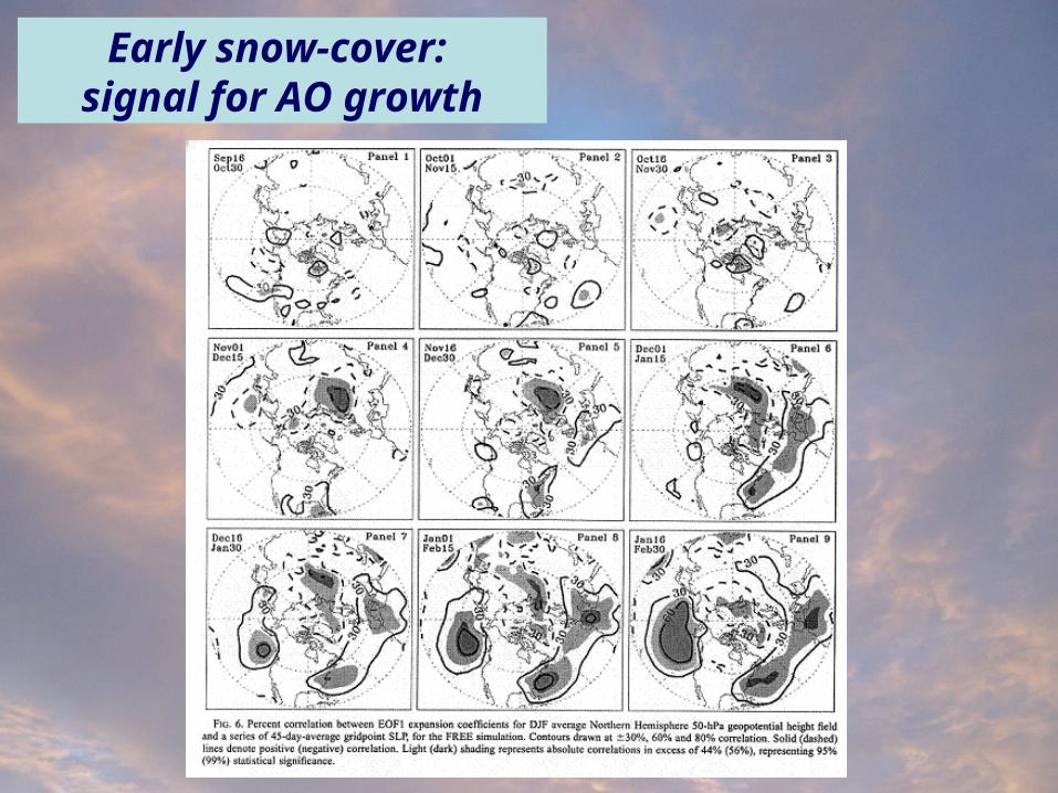
Early snow-cover: signal for AO growth

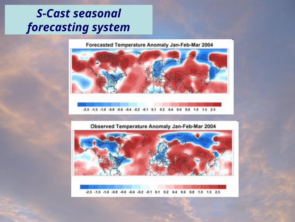
S-Cast seasonal forecasting system

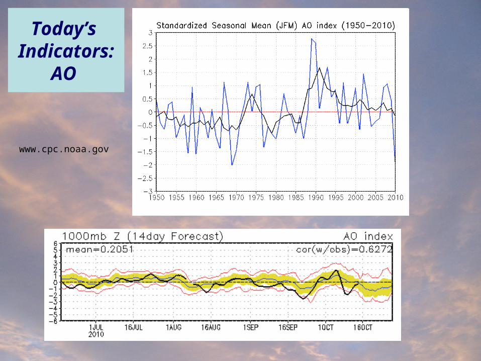
Today’s Indicators:

AO

www.cpc.noaa.gov

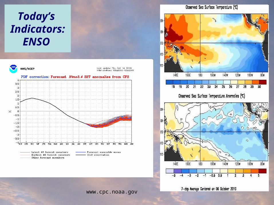
Today’s Indicators:

ENSO

www.cpc.noaa.gov

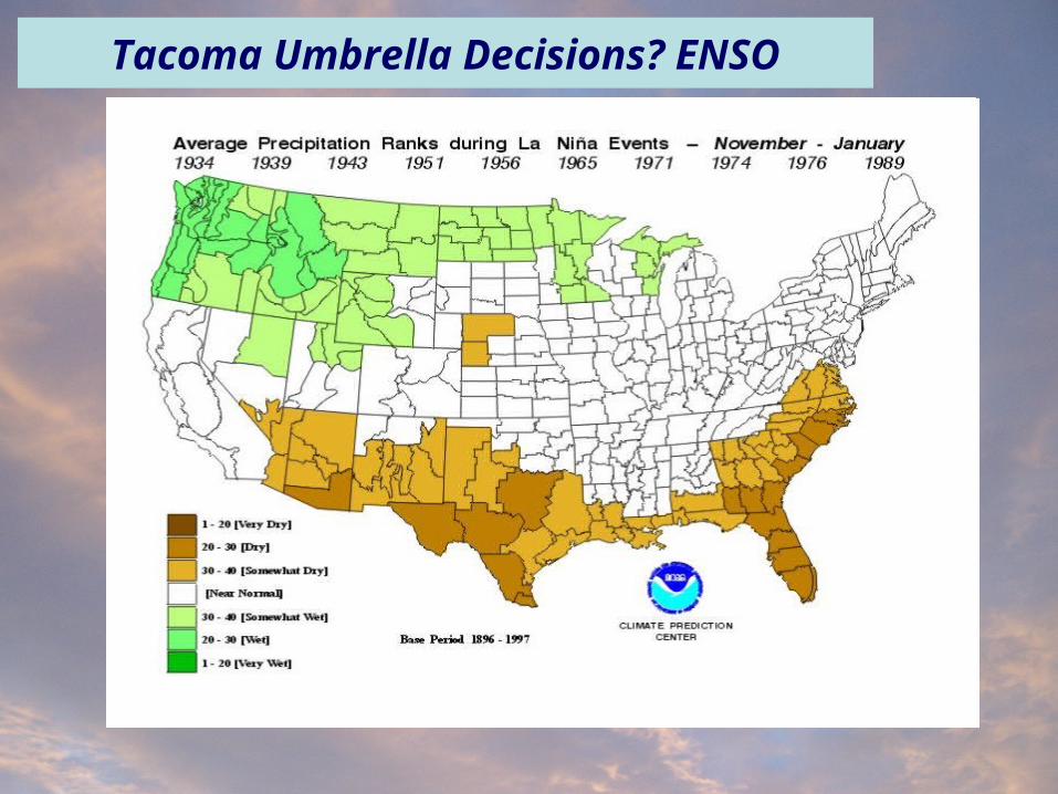
Tacoma Umbrella Decisions? ENSO

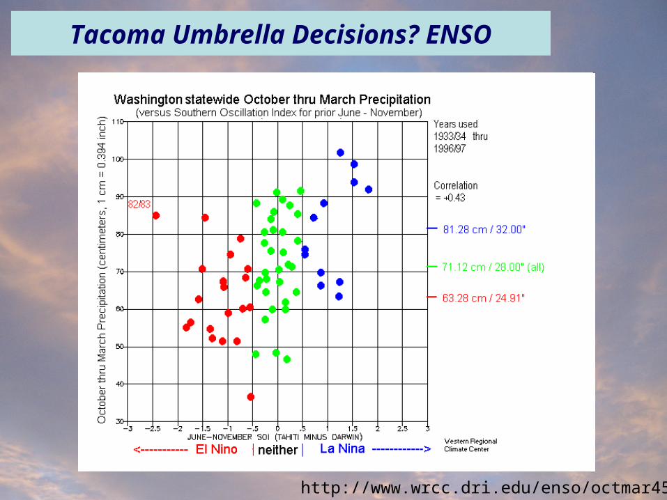
Tacoma Umbrella Decisions? ENSO

http://www.wrcc.dri.edu/enso/octmar45.gif

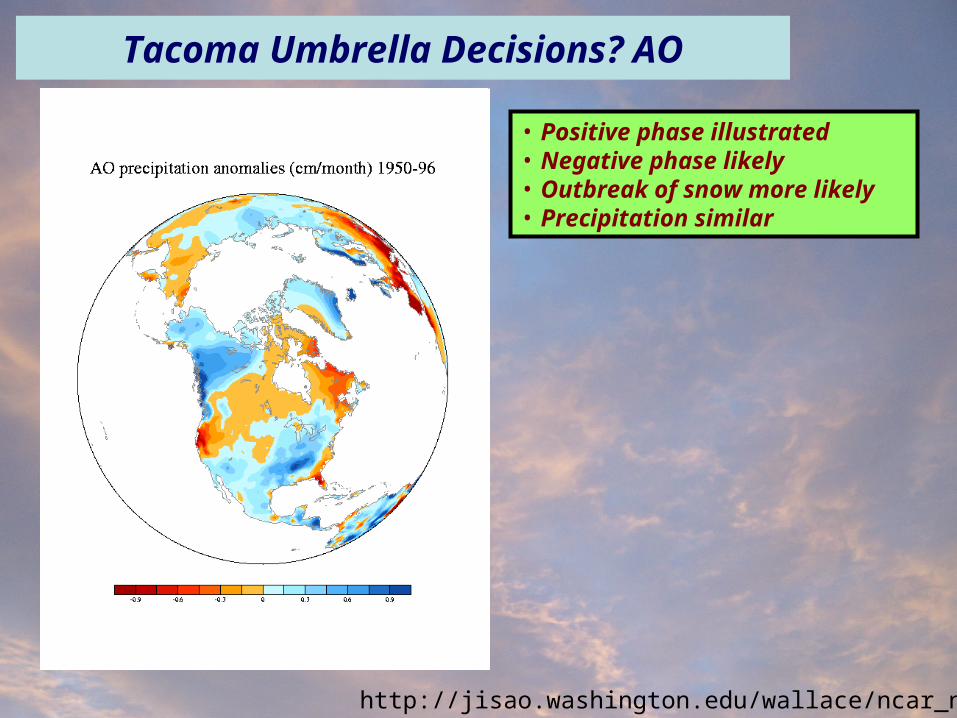
Tacoma Umbrella Decisions? AO

http://jisao.washington.edu/wallace/ncar_notes/

• Positive phase illustrated• Negative phase likely• Outbreak of snow more likely• Precipitation similar

Precip. % depart.

Prob. of % depart. Profit $ % return

Put payout

Expected payout

Profit $ with put

% return with put

-30% 0.01 -20000 -16.67% 31825 318.25 5412.5 4.51%

-25% 0.02 -11275 -9.40% 27075 541.5 9387.5 7.83%

-20% 0.03 -5375 -4.35% 22325 669.75 10537.5 8.52%

-15% 0.1 1125 0.88% 17575 1757.5 12287.5 9.67%

-10% 0.11 6900 5.36% 12825 1410.75 13312.5 10.34%

-5% 0.13 18375 13.76% 8075 1049.75 20037.5 15.01%

0% 0.2 26000 18.87% 3325 665 22912.5 16.63%

5% 0.15 56000 39.22% 0 0 49587.5 34.73%

10% 0.08 82875 53.68% 0 0 76462.5 49.53%

15% 0.06 102200 60.87% 0 0 95787.5 57.05%

20% 0.04 113575 64.84% 0 0 107162.5 61.17%

25% 0.03 140000 77.78% 0 0 133587.5 74.22%

30% 0.02 149650 82.02% 0 0 143237.5 78.51%

35% 0.01 161700 88.51% 0 0 155287.5 85.00%

40% 0.01 180625 100.00% 0 0 174212.5 96.45%

Tacoma Umbrella Decisions?

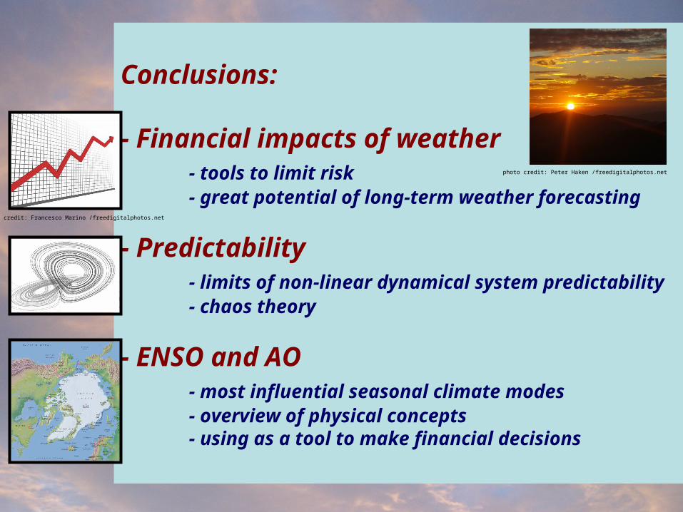
Conclusions:

- Financial impacts of weather- tools to limit risk- great potential of long-term weather forecasting

- Predictability- limits of non-linear dynamical system predictability- chaos theory

- ENSO and AO- most influential seasonal climate modes- overview of physical concepts- using as a tool to make financial decisions

photo credit: Peter Haken /freedigitalphotos.net

photo credit: Francesco Marino /freedigitalphotos.net