Seasonal & Interannual Variability in Tropospheric CO: Global-Scale Analysis of GEOS-CHEM
Seasonal changes in the tropospheric carbon monoxide profile over the remote Southern Hemisphere evaluated using multi-model simulations and aircraft observations
Jenny A. Fisher, Stephen R. Wilson University of Wollongong
Guang Zeng National Institute of Water and Atmospheric Research
Jason E. Williams Royal Netherlands Meteorological Institute
Louisa K. Emmons National Center for Atmospheric Research
Ray L. Langenfelds, Paul B. Krummel, L. Paul Steele CSIRO Oceans and Atmosphere Flagship
ACCOMC 12 November 2014
Jenny A. Fisher ([email protected]) 2014 ACCOMC
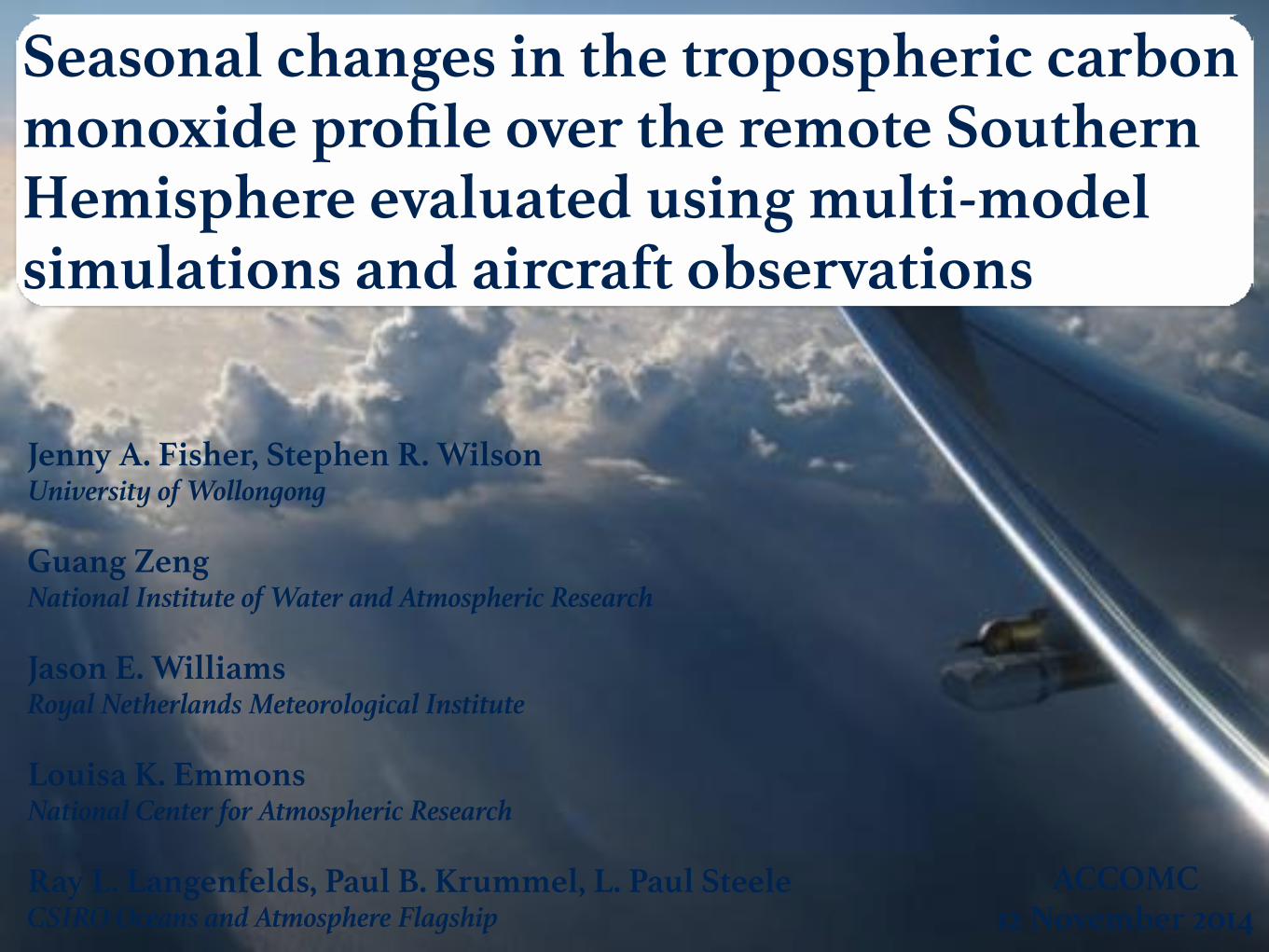
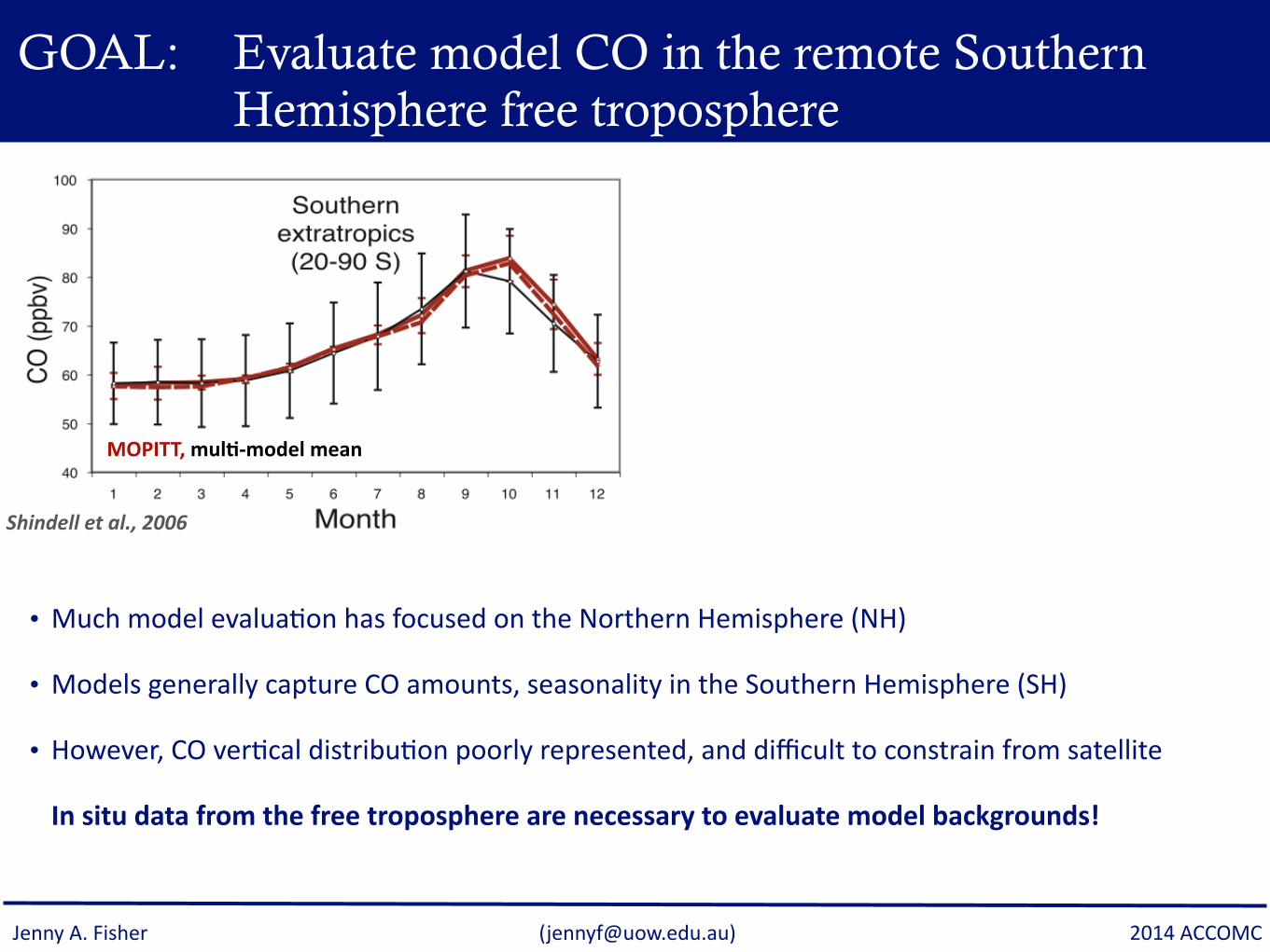
GOAL: Evaluate model CO in the remote Southern Hemisphere free troposphere
• Much model evaluaCon has focused on the Northern Hemisphere (NH)
• Models generally capture CO amounts, seasonality in the Southern Hemisphere (SH)
• However, CO verCcal distribuCon poorly represented, and difficult to constrain from satellite
In situ data from the free troposphere are necessary to evaluate model backgrounds!
MOPITT, mul>-‐model mean
Shindell et al., 2006

Jenny A. Fisher ([email protected]) 2014 ACCOMC
GOAL: Evaluate model CO in the remote Southern Hemisphere free troposphere
• Much model evaluaCon has focused on the Northern Hemisphere (NH)
• Models generally capture CO amounts, seasonality in the Southern Hemisphere (SH)
• However, CO verCcal distribuCon poorly represented, and difficult to constrain from satellite
In situ data from the free troposphere are necessary to evaluate model backgrounds!
MOPITT, mul>-‐model mean
Ra>o of CO(350 hPa) / CO(850hPa)
MOPITT
Mul>-‐model mean
Shindell et al., 2006

Jenny A. Fisher ([email protected]) 2014 ACCOMC
50°S
40°S
30°S
20°S
10°S
150°E 180° 150° W 120° W 90°W
CGOP
HIPPO
Aircraft data provide a unique opportunity
Cape Grim Overflight Program (CGOP) • 1991-‐1999, ~monthly flights • Melbourne —> Bass Strait —> Cape Grim • 0-‐8 km profiles west of Cape Grim • 85 flights total, ~17-‐20 flasks per flight
HIAPER Pole-‐to-‐Pole Observa>ons (HIPPO) • 2009-‐2011, 5 deployments • ArcCc —> Pacific —> AntarcCc • ConCnuous 0-‐8 km profiles • 4-‐6 SH flights/deployment, conCnuous sampling

Jenny A. Fisher ([email protected]) 2014 ACCOMC
GEOS−Chem
45oS
40oS
35oS
140oE 150oE
NIWA−UKCA
45oS
40oS
35oS
140oE 150oE
45oS
40oS
35oS
140oE 150oE
TM5 CAM−chem
45oS
40oS
35oS
140oE 150oE
40 50 60 70 80 ppbv
SHMIP: Southern Hemisphere Model Intercomparison Project
4 atmospheric chemistry models • GEOS-‐Chem • NIWA-‐UKCA • TM5 • CAM-‐chem
5-‐year simula>on (2004-‐2008)
Iden>cal emissions* • MACCity-‐REAS fossil fuels • GFEDv3 biomass burning • MEGANv2.1-‐CLM biogenic • *except parameterised lightning NOx, soil NOx, volcanic SO2
Different chemistry, meteorology

Jenny A. Fisher ([email protected]) 2014 ACCOMC
20
40
60
80
100
CO
(ppbv)
n=
35
n=
35
n=
25
n=
40
n=
22
n=
17
n=
26
n=
31
n=
37
n=
36
n=
31
n=
26
20
40
60
80
100
CO
(ppbv)
n=
60
n=
53
n=
39
n=
40
n=
35
n=
27
n=
32
n=
53
n=
65
n=
52
n=
51
n=
44
1 2 3 4 5 6 7 8 9 10 11 12
Month
20
40
60
80
100
CO
(ppbv)
n=
80
n=
87
n=
39
n=
54
n=
42
n=
21
n=
40
n=
57
n=
59
n=
56
n=
75
n=
49
0-2 km
2-5 km
5-8 km
Observations
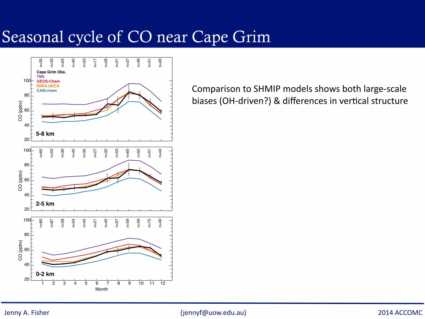
Seasonal cycle of CO near Cape Grim
Jenny A. Fisher ([email protected]) 2014 ACCOMC
20
40
60
80
100
CO
(ppbv)
n=
35
n=
35
n=
25
n=
40
n=
22
n=
17
n=
26
n=
31
n=
37
n=
36
n=
31
n=
26
20
40
60
80
100
CO
(ppbv)
n=
60
n=
53
n=
39
n=
40
n=
35
n=
27
n=
32
n=
53
n=
65
n=
52
n=
51
n=
44
1 2 3 4 5 6 7 8 9 10 11 12
Month
20
40
60
80
100
CO
(ppbv)
n=
80
n=
87
n=
39
n=
54
n=
42
n=
21
n=
40
n=
57
n=
59
n=
56
n=
75
n=
49
0-2 km
2-5 km
5-8 km
Cape Grim Obs.
TM5
GEOS-Chem
NIWA-UKCA
CAM-chem
Seasonal cycle of CO near Cape Grim
Comparison to SHMIP models shows both large-‐scale biases (OH-‐driven?) & differences in verCcal structure

Jenny A. Fisher ([email protected]) 2014 ACCOMC
20
40
60
80
100
CO
(ppbv)
n=
35
n=
35
n=
25
n=
40
n=
22
n=
17
n=
26
n=
31
n=
37
n=
36
n=
31
n=
26
20
40
60
80
100
CO
(ppbv)
n=
60
n=
53
n=
39
n=
40
n=
35
n=
27
n=
32
n=
53
n=
65
n=
52
n=
51
n=
44
1 2 3 4 5 6 7 8 9 10 11 12
Month
20
40
60
80
100
CO
(ppbv)
n=
80
n=
87
n=
39
n=
54
n=
42
n=
21
n=
40
n=
57
n=
59
n=
56
n=
75
n=
49
0-2 km
2-5 km
5-8 km
Cape Grim Obs.
TM5
GEOS-Chem
NIWA-UKCA
CAM-chem
Seasonal cycle of CO near Cape Grim
TM5 overesCmates
Comparison to SHMIP models shows both large-‐scale biases (OH-‐driven?) & differences in verCcal structure

Jenny A. Fisher ([email protected]) 2014 ACCOMC
20
40
60
80
100
CO
(ppbv)
n=
35
n=
35
n=
25
n=
40
n=
22
n=
17
n=
26
n=
31
n=
37
n=
36
n=
31
n=
26
20
40
60
80
100
CO
(ppbv)
n=
60
n=
53
n=
39
n=
40
n=
35
n=
27
n=
32
n=
53
n=
65
n=
52
n=
51
n=
44
1 2 3 4 5 6 7 8 9 10 11 12
Month
20
40
60
80
100
CO
(ppbv)
n=
80
n=
87
n=
39
n=
54
n=
42
n=
21
n=
40
n=
57
n=
59
n=
56
n=
75
n=
49
0-2 km
2-5 km
5-8 km
Cape Grim Obs.
TM5
GEOS-Chem
NIWA-UKCA
CAM-chem
Seasonal cycle of CO near Cape Grim
TM5 overesCmatesCAM-‐chem underesCmates
Comparison to SHMIP models shows both large-‐scale biases (OH-‐driven?) & differences in verCcal structure

Jenny A. Fisher ([email protected]) 2014 ACCOMC
20
40
60
80
100
CO
(ppbv)
n=
35
n=
35
n=
25
n=
40
n=
22
n=
17
n=
26
n=
31
n=
37
n=
36
n=
31
n=
26
20
40
60
80
100
CO
(ppbv)
n=
60
n=
53
n=
39
n=
40
n=
35
n=
27
n=
32
n=
53
n=
65
n=
52
n=
51
n=
44
1 2 3 4 5 6 7 8 9 10 11 12
Month
20
40
60
80
100
CO
(ppbv)
n=
80
n=
87
n=
39
n=
54
n=
42
n=
21
n=
40
n=
57
n=
59
n=
56
n=
75
n=
49
0-2 km
2-5 km
5-8 km
Cape Grim Obs.
TM5
GEOS-Chem
NIWA-UKCA
CAM-chem
Seasonal cycle of CO near Cape Grim
TM5 overesCmatesCAM-‐chem underesCmatesGEOS-‐Chem, NIWA-‐UKCA reasonable… but with differences in verCcal structure
Comparison to SHMIP models shows both large-‐scale biases (OH-‐driven?) & differences in verCcal structure
We use the CO ver>cal gradient as a metric for model evalua>on
Jenny A. Fisher ([email protected]) 2014 ACCOMC
0
2
4
6
8
Altitude (
km
)
DJF MAMJ
0 10 20∆CO (ppbv)
JA SONCGOPHIPPO
0 10 20∆CO (ppbv)
0 10 20∆CO (ppbv)
0 10 20∆CO (ppbv)
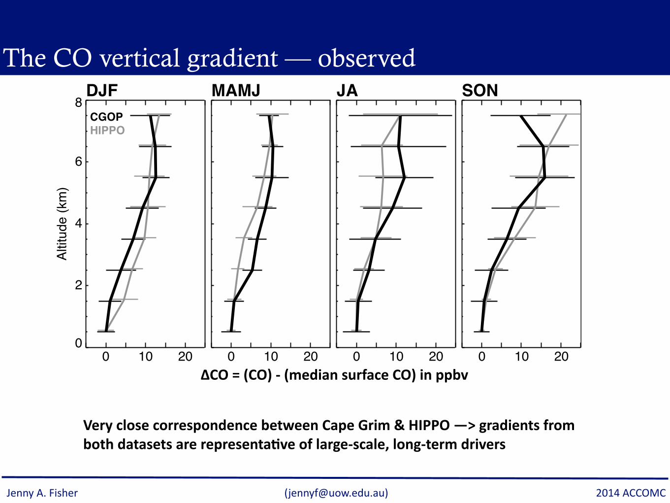
The CO vertical gradient — observed
ΔCO = (CO) -‐ (median surface CO) in ppbv
Very close correspondence between Cape Grim & HIPPO —> gradients from both datasets are representa>ve of large-‐scale, long-‐term drivers

Jenny A. Fisher ([email protected]) 2014 ACCOMC
0
2
4
6
8
Altitu
de
(km
)
n=135
n=81
n=32
n=42
n=79
n=31
n=30
n=35DJF
n=102
n=54
n=35
n=34
n=70
n=28
n=32
n=44MAMJ
−5 0 5 10 15 20 25∆CO (ppbv)
0
2
4
6
8
Altitu
de
(km
)
n=65
n=32
n=17
n=18
n=49
n=20
n=20
n=17JA
−5 0 5 10 15 20 25∆CO (ppbv)
n=132
n=58
n=40
n=42
n=86
n=34
n=35
n=35SONCape Grim Obs.
TM5
GEOS-Chem
NIWA-UKCA
CAM-chem
The CO vertical gradient — observed & modelled
In austral winter/spring, all models reproduce verCcal gradient of 1.9-‐2.2 ppbv km-‐1 driven by primary biomass burning emissions

Jenny A. Fisher ([email protected]) 2014 ACCOMC
0
2
4
6
8
Altitu
de
(km
)
n=135
n=81
n=32
n=42
n=79
n=31
n=30
n=35DJF
n=102
n=54
n=35
n=34
n=70
n=28
n=32
n=44MAMJ
−5 0 5 10 15 20 25∆CO (ppbv)
0
2
4
6
8
Altitu
de
(km
)
n=65
n=32
n=17
n=18
n=49
n=20
n=20
n=17JA
−5 0 5 10 15 20 25∆CO (ppbv)
n=132
n=58
n=40
n=42
n=86
n=34
n=35
n=35SONCape Grim Obs.
TM5
GEOS-Chem
NIWA-UKCA
CAM-chem
The CO vertical gradient — observed & modelled
In austral summer/autumn, most models underes>mate verCcal gradient of ~1.6-‐1.9 ppbv km-‐1 and show a wider inter-‐model spread.
WHY?
0
2
4
6
8
Altitu
de
(km
)
n=135
n=81
n=32
n=42
n=79
n=31
n=30
n=35DJF
n=102
n=54
n=35
n=34
n=70
n=28
n=32
n=44MAMJ
−5 0 5 10 15 20 25∆CO (ppbv)
0
2
4
6
8
Altitu
de
(km
)
n=65
n=32
n=17
n=18
n=49
n=20
n=20
n=17JA
−5 0 5 10 15 20 25∆CO (ppbv)
n=132
n=58
n=40
n=42
n=86
n=34
n=35
n=35SONCape Grim Obs.
TM5
GEOS-Chem
NIWA-UKCA
CAM-chem
Jenny A. Fisher ([email protected]) 2014 ACCOMC
∆CO (ppbv)
0
2
4
6
8
Altit
ude
(km
)
b. Fixed-lifetime CO25 tracerDJF MAMJ JA SON
0 10 20 0 10 200 10 200 10 20
0
2
4
6
8
Altit
ude
(km
)
d. LPJ-GUESS biogenic emissionsDJF MAMJ JA SON
0 10 20 0 10 200 10 200 10 20
a. Standard simulation
0
2
4
6
8
Altit
ude
(km
)
DJF MAMJ JA SON
0 10 20 0 10 200 10 200 10 20
0
2
4
6
8
Altit
ude
(km
)
c. OH-loss COOH tracerDJF MAMJ JA SON
0 10 20 0 10 200 10 200 10 20
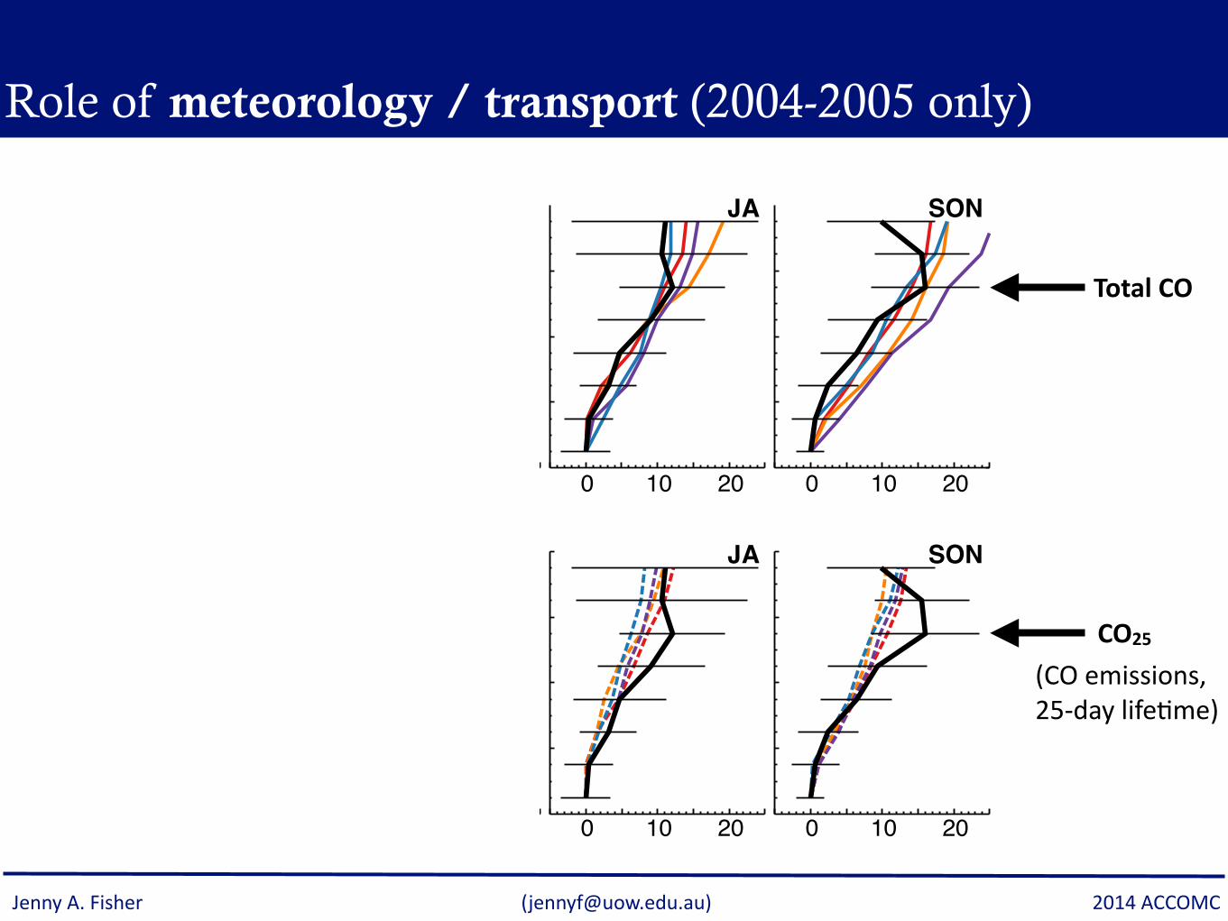
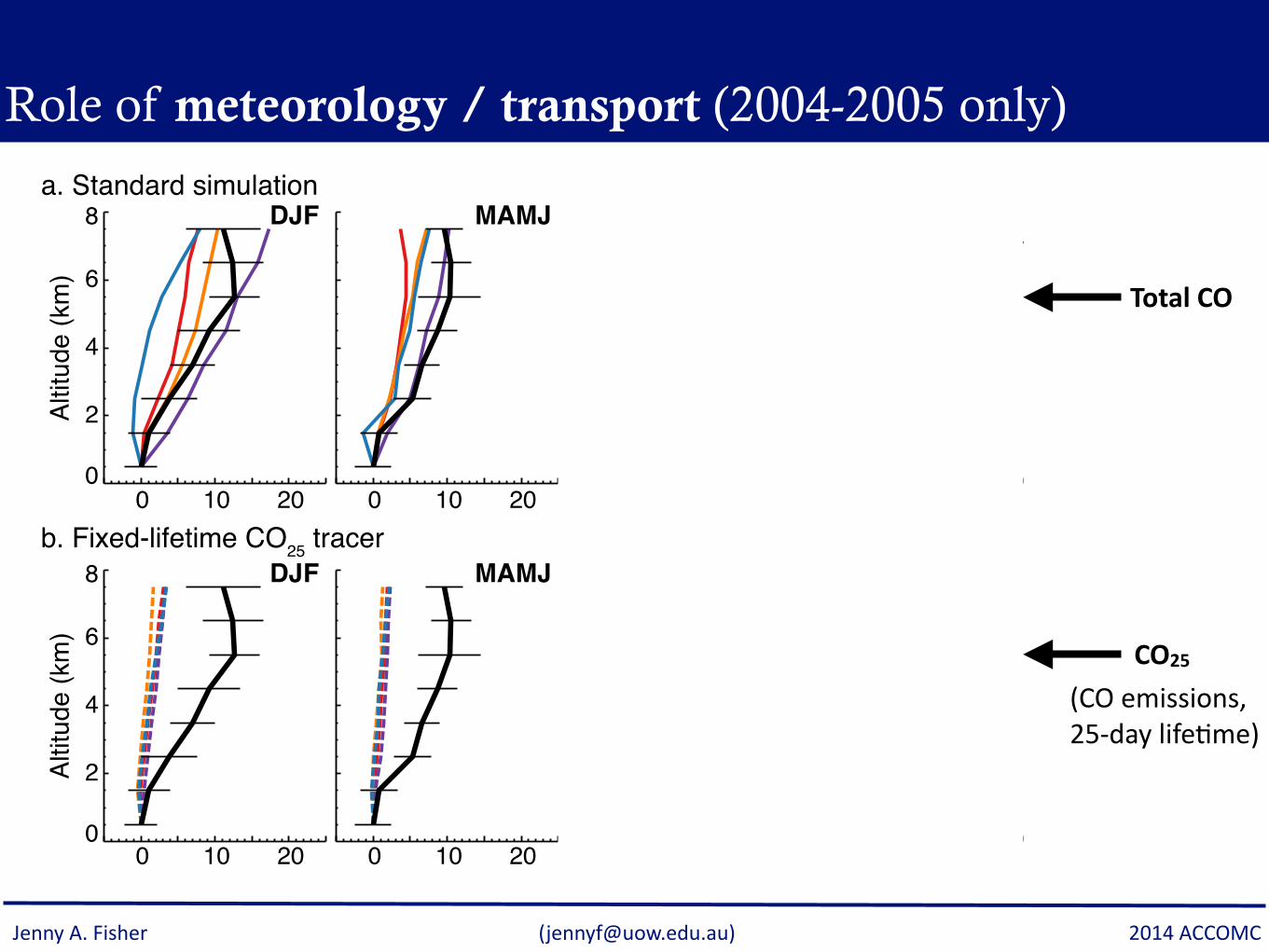
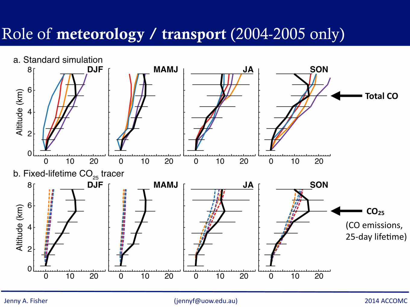
Role of meteorology / transport (2004-2005 only)
Total CO
CO25
(CO emissions, 25-‐day lifeCme)
Jenny A. Fisher ([email protected]) 2014 ACCOMC
∆CO (ppbv)
0
2
4
6
8
Altit
ude
(km
)
b. Fixed-lifetime CO25 tracerDJF MAMJ JA SON
0 10 20 0 10 200 10 200 10 20
0
2
4
6
8
Altit
ude
(km
)
d. LPJ-GUESS biogenic emissionsDJF MAMJ JA SON
0 10 20 0 10 200 10 200 10 20
a. Standard simulation
0
2
4
6
8
Altit
ude
(km
)
DJF MAMJ JA SON
0 10 20 0 10 200 10 200 10 20
0
2
4
6
8
Altit
ude
(km
)
c. OH-loss COOH tracerDJF MAMJ JA SON
0 10 20 0 10 200 10 200 10 20
Role of meteorology / transport (2004-2005 only)
Total CO
CO25
(CO emissions, 25-‐day lifeCme)

Jenny A. Fisher ([email protected]) 2014 ACCOMC
∆CO (ppbv)
0
2
4
6
8
Altit
ude
(km
)
b. Fixed-lifetime CO25 tracerDJF MAMJ JA SON
0 10 20 0 10 200 10 200 10 20
0
2
4
6
8
Altit
ude
(km
)
d. LPJ-GUESS biogenic emissionsDJF MAMJ JA SON
0 10 20 0 10 200 10 200 10 20
a. Standard simulation
0
2
4
6
8
Altit
ude
(km
)
DJF MAMJ JA SON
0 10 20 0 10 200 10 200 10 20
0
2
4
6
8
Altit
ude
(km
)
c. OH-loss COOH tracerDJF MAMJ JA SON
0 10 20 0 10 200 10 200 10 20
Role of chemical loss (2004-2005 only)
Total CO
COOH
(CO emissions, OH-‐driven loss)

Jenny A. Fisher ([email protected]) 2014 ACCOMC
∆CO (ppbv)
0
2
4
6
8
Altit
ude
(km
)
b. Fixed-lifetime CO25 tracerDJF MAMJ JA SON
0 10 20 0 10 200 10 200 10 20
0
2
4
6
8
Altit
ude
(km
)
d. LPJ-GUESS biogenic emissionsDJF MAMJ JA SON
0 10 20 0 10 200 10 200 10 20
a. Standard simulation
0
2
4
6
8
Altit
ude
(km
)
DJF MAMJ JA SON
0 10 20 0 10 200 10 200 10 20
0
2
4
6
8
Altit
ude
(km
)
c. OH-loss COOH tracerDJF MAMJ JA SON
0 10 20 0 10 200 10 200 10 20
∆CO (ppbv)
0
2
4
6
8
Altit
ude
(km
)
b. Fixed-lifetime CO25 tracerDJF MAMJ JA SON
0 10 20 0 10 200 10 200 10 20
0
2
4
6
8
Altit
ude
(km
)
d. LPJ-GUESS biogenic emissionsDJF MAMJ JA SON
0 10 20 0 10 200 10 200 10 20
a. Standard simulation
0
2
4
6
8
Altit
ude
(km
)
DJF MAMJ JA SON
0 10 20 0 10 200 10 200 10 20
0
2
4
6
8
Altit
ude
(km
)
c. OH-loss COOH tracerDJF MAMJ JA SON
0 10 20 0 10 200 10 200 10 20
Role of biogenic sources (2004-2005 only)
Total CO
Total COLPJ-‐GUESS isoprene
MEGAN-‐CLM isoprene

Jenny A. Fisher ([email protected]) 2014 ACCOMC
a. CO
0
100
200 ppbGEOS−Chem NIWA-UKCA
c. CH2O
0
2.5
5 ppb
0
5
10 ppb
b. Isoprene
0
6
12
e. HO2
d. OH
0
100
200 ppq
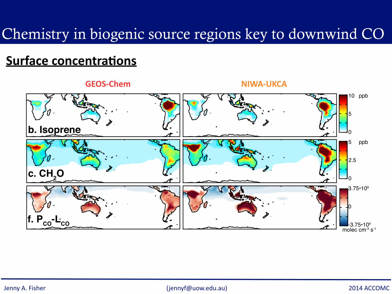
f. PCO-LCO -3.75•106
0
3.75•106
molec cm-3 s-1
ppt
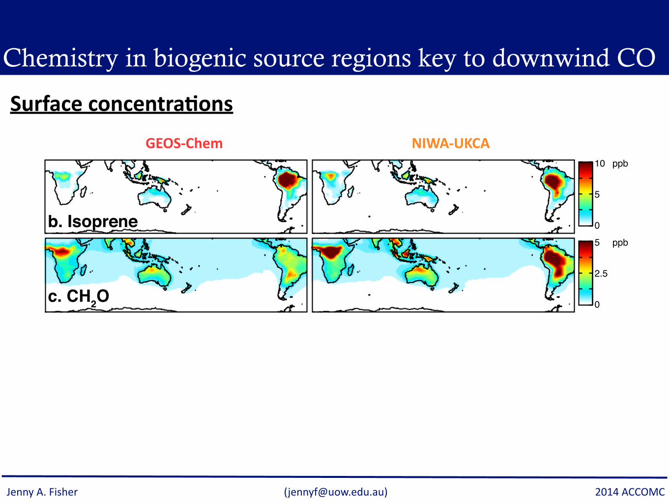
Chemistry in biogenic source regions key to downwind CO
Surface concentra>onsGEOS-‐Chem NIWA-‐UKCA
Jenny A. Fisher ([email protected]) 2014 ACCOMC
a. CO
0
100
200 ppbGEOS−Chem NIWA-UKCA
c. CH2O
0
2.5
5 ppb
0
5
10 ppb
b. Isoprene
0
6
12
e. HO2
d. OH
0
100
200 ppq
f. PCO-LCO -3.75•106
0
3.75•106
molec cm-3 s-1
ppt
Chemistry in biogenic source regions key to downwind CO
Surface concentra>onsa. CO
0
100
200 ppbGEOS−Chem NIWA-UKCA
c. CH2O
0
2.5
5 ppb
0
5
10 ppb
b. Isoprene
0
6
12
e. HO2
d. OH
0
100
200 ppq
f. PCO-LCO -3.75•106
0
3.75•106
molec cm-3 s-1
ppt
GEOS-‐Chem NIWA-‐UKCA
Jenny A. Fisher ([email protected]) 2014 ACCOMC
a. CO
0
100
200 ppbGEOS−Chem NIWA-UKCA
c. CH2O
0
2.5
5 ppb
0
5
10 ppb
b. Isoprene
0
6
12
e. HO2
d. OH
0
100
200 ppq
f. PCO-LCO -3.75•106
0
3.75•106
molec cm-3 s-1
ppt
Chemistry in biogenic source regions key to downwind CO
Surface concentra>onsa. CO
0
100
200 ppbGEOS−Chem NIWA-UKCA
c. CH2O
0
2.5
5 ppb
0
5
10 ppb
b. Isoprene
0
6
12
e. HO2
d. OH
0
100
200 ppq
f. PCO-LCO -3.75•106
0
3.75•106
molec cm-3 s-1
ppt
a. CO
0
100
200 ppbGEOS−Chem NIWA-UKCA
c. CH2O
0
2.5
5 ppb
0
5
10 ppb
b. Isoprene
0
6
12
e. HO2
d. OH
0
100
200 ppq
f. PCO-LCO -3.75•106
0
3.75•106
molec cm-3 s-1
ppt
GEOS-‐Chem NIWA-‐UKCA
Second & later stages of isoprene oxida>on chemistry proceed faster in NIWA-‐UKCA than in GEOS-‐Chem —> less downwind CO produc>on at low alCtude

Jenny A. Fisher ([email protected]) 2014 ACCOMC
c. CO
b. CH2O
a. Isoprene
−90 0 90Longitude
4
8
12
Altit
ude
(km
)
0
GEOS−Chem
0
100
200 ppt
−90 0 90Longitude
NIWA-UKCA
0
250
500 ppt
−90 0 90Longitude
−90 0 90Longitude
4
8
12
Altit
ude
(km
)
0
0
50
100 ppb
−90 0 90Longitude
−90 0 90Longitude
4
8
12
Altit
ude
(km
)
0
1 2 3 1 2 3
Transport of biogenic-sourced CO also critical
GEOS-‐Chem NIWA-‐UKCA15-‐45°S cross-‐sec>ons
S. America
Africa
Australia
CGOP Profiles
NIWA-‐UKCA vs GEOS-‐Chem:
More deep convecCve injecCon of isoprene over South American max
More UT producCon of CH2O and subsequently CO

Jenny A. Fisher ([email protected]) 2014 ACCOMC
c. CO
b. CH2O
a. Isoprene
−90 0 90Longitude
4
8
12
Altit
ude
(km
)
0
GEOS−Chem
0
100
200 ppt
−90 0 90Longitude
NIWA-UKCA
0
250
500 ppt
−90 0 90Longitude
−90 0 90Longitude
4
8
12
Altit
ude
(km
)
0
0
50
100 ppb
−90 0 90Longitude
−90 0 90Longitude
4
8
12
Altit
ude
(km
)
0
1 2 3 1 2 3
Transport of biogenic-sourced CO also critical
GEOS-‐Chem NIWA-‐UKCA15-‐45°S cross-‐sec>ons
S. America
Africa
Australia
CGOP Profiles
NIWA-‐UKCA vs GEOS-‐Chem:
More deep convecCve injecCon of isoprene over South American max
More zonal transport of CO to UT regions downwind
More UT producCon of CH2O and subsequently CO

Jenny A. Fisher ([email protected]) 2014 ACCOMC
What’s next for SHMIP?• Fisher et al. (this work) in ACPD now: www.atmos-‐chem-‐phys-‐discuss.net/14/27531/2014/
• Zeng et al. in prep., focus impact of biogenic emissions on CO from surface in situ and ground-‐based total column measurements
• Jason Williams (KNMI) invesCgaCng sensiCvity of NOY in UTLS to biogenic emissions
• Kaitlyn Lieschke (UOW, 2015 Honours student) evaluaCng UT NOX and O3 to invesCgate impacts of model differences in lightning NOX parameterisaCons.
SHADOZGEOS−ChemCAM−ChemNIWA−UKCATM5
January
0 100
O3 (ppb)
1000
800
600
400
200
0
Pre
ssu
re (
hP
a)
April July October
0 100 0 100 0 100
San Cristobal ozonesonde
Jenny A. Fisher ([email protected]) 2014 ACCOMC
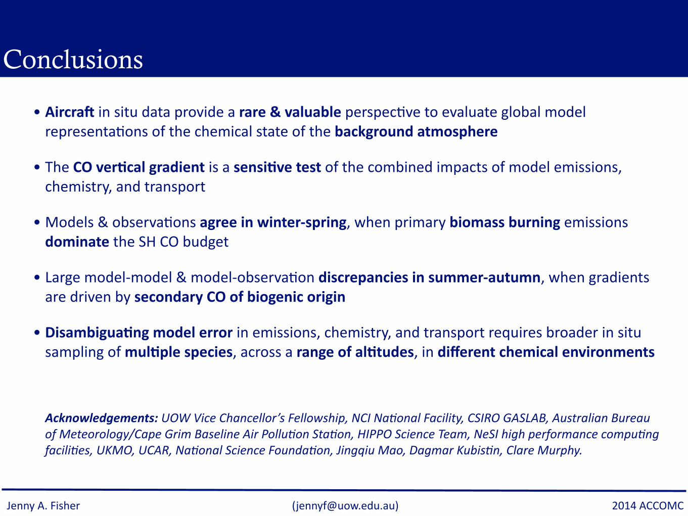
Conclusions
• Aircrai in situ data provide a rare & valuable perspecCve to evaluate global model representaCons of the chemical state of the background atmosphere
• The CO ver>cal gradient is a sensi>ve test of the combined impacts of model emissions, chemistry, and transport
• Models & observaCons agree in winter-‐spring, when primary biomass burning emissions dominate the SH CO budget
• Large model-‐model & model-‐observaCon discrepancies in summer-‐autumn, when gradients are driven by secondary CO of biogenic origin
• Disambigua>ng model error in emissions, chemistry, and transport requires broader in situ sampling of mul>ple species, across a range of al>tudes, in different chemical environments
Acknowledgements: UOW Vice Chancellor’s Fellowship, NCI Na8onal Facility, CSIRO GASLAB, Australian Bureau of Meteorology/Cape Grim Baseline Air Pollu8on Sta8on, HIPPO Science Team, NeSI high performance compu8ng facili8es, UKMO, UCAR, Na8onal Science Founda8on, Jingqiu Mao, Dagmar Kubis8n, Clare Murphy.