Search for primes of the form m2 + 1

Marek Wolf

Group of Mathematical Methods in Physics, University of Wroc lawPl.Maxa Borna 9, PL-50-204 Wroc law, Poland

e-mail: mwolf@ift.uni.wroc.pl

Abstract

The results of the computer hunt for the primes of the form q = m2 + 1up to 1020 are reported. The number of sign changes of the differenceπq(x) − Cq

2

∫ x2

du√u log(u)

and the error term for this difference is investi-

gated. The analogs of the Brun’s constant and the Skewes number arecalculated. An analog of the B conjecture of Hardy–Littlewood is for-mulated. It is argued that there is no Chebyshev bias for primes of theform q = m2 + 1. All encountered integrals we were able to express bythe logarithmic integral.

Mathematics Subject Classification: 11L20, 11N13, 11N32, 11A41, 11N05, 11Y35,11Y60

1 Introduction

This paper is devoted to investigation of the set of prime numbers

Q = {2, 5, 17, 37, 101, 197, 257, 401, 577 . . .} (1)

given by the quadratic polynomial m2 + 1 and let qn denote the n-th prime of thisform. By the conjecture E of Hardy and Littlewood [19] the number1 πq(x) of primesq < x of the form q = m2 + 1 is given by

πq(x) ∼ Cq

√x

log(x), (2)

where

Cq =∏p≥3

(1− (−1)(p−1)/2

p− 1

)= 1.372813462818246009112192696727 . . . (3)

The primes qn were investigated in the past both theoretically and numerically. Oneof the strongest theoretical results is the theorem of H. Iwaniec [22], who proved thatthere exist infinitely many integers m2 + 1 which are 2-almost-primes. In 1998 H.

1 we adopt here the convention that all functions describing usual prime numbers will have thesubscript q when applied to primes of the form q = m2 + 1

arX

iv:0

803.

1456

v3 [

mat

h.N

T]

27

Jan

2010

2 1 Introduction

Iwaniec and J. Friedlander [15] have proved that there is an infinity of primes givenby the polynomial of two variables m,n of the form m2 + n4, thus the case of thepolynomial of one variable m2 + 1 is not covered by their theorem. Quite recentlythere appeared two papers by S. Baier and L. Zhao [2, 3], treating the more generalproblem of the primes of the form m2 + k in average over square-free parameterk in appropriate intervals. In the computational part we should cite the papersby Shanks [38, 36] and Wunderlich [42]; in the last paper the table of πq(x) forx < 1.96× 1014 is given.

By analogy with the case of all primes, where substitution of the logarithmicintegral Li(x) =

∫ x2du/ log(u) instead of x/ log(x) gives better approximation for

π(x), we recast the original Hardy and Littlewood conjecture E in the form:

πq(x) ∼ 1

2Cq

∫ x

2

du√u log u

(4)

= Cq

( √x

log x+

2√x

log2 x+

8√x

log3 x+

48√x

log4 x+ . . .+

2n−1(n− 1)!√x

logn x+ . . .

).

The series in parenthesis above is asymptotic one: the terms initially decrease,but for sufficiently large n they become to increase. Thus this series has to be cut atsuch n0, which depends on x, that the n0-th term (and consecutive terms) is largerthan previous one with n0(x) − 1 what gives for the threshold at which the series(4) should be cut the inequality:

n0(x) >1

2log(x) + 1. (5)

Besides this asymptotic representation the integral (4) can be linked to the logarith-mic integral by the change of variables u = t2:∫ b

a

du√u log u

=

∫ √b√a

dt

log t= li(√b)− li(

√a). (6)

Here we use the following convention for the lower limit of integration:

li(x) = v.p.

∫ x

0

du

log(u)= lim

ε→0

(∫ 1−ε

0

du

log(u)+

∫ x

1+ε

du

log(u)

)(7)

Integration by parts gives the asymptotic expansion:

li(x) ∼ x

log(x)+

x

log2(x)+

2x

log3(x)+

6x

log4(x)+ · · · n!x

logn+1(x). (8)

which should be cut at n0 = log(x). There is a series giving li(x) for all x andquickly convergent which has n! in denominator and logn(x) in nominator insteadof opposite order in (8) (see [1, Sect. 5.1])

li(x) = γ + log log(x) +∞∑n=1

logn(x)

n · n!for x > 1 , (9)

3

Here γ = 0.57721566490153286... is the Euler-Mascheroni constant. Even fasterconverging series was discovered by Ramanujan [6, p.123]:

li(x) = γ+log(log(x))+√x

∞∑n=1

(−1)n−1(log(x))n

n! 2n−1

b(n−1)/2c∑k=0

1

2k + 1for x > 1 . (10)

Skipping the number 2 = 12 + 1 all odd primes qn can be expressed by the formm2 + 1 only for m even, thus we put m = 2k, i.e. we are looking for primes of theform 4k2 + 1. We have collected in one file of the size roughly 3.5 GB values ofk (thus the prime 2 = 12 + 1 is absent here!) up to k = 4999999978 what corre-sponds to all primes of the form m2 + 1 < 1020. The compressed data occupies 760MB and is available for downloading from http://www.ift.uni.wroc.pl/~mwolf/

4k-2+1-data.zip. Initially up to 6.65× 1016 I have used my own program writtenin Fortran for Alpha DEC workstation, but to reach 1020 we have used the free pack-age PARI/GP [39] developed especially for number theoretical purposes. To scanthe interval (6.65 × 1016, 1020) it took about 10 days of CPU time on the PC withthe clock 2.5 GHz using the built-in PARI very fast function isprime(p). The TableI gives comparison of πq(x) with conjectures (2) and (4). Among those 312,357,934values of k there were 11,864,645 such k that they in turn were primes, i.e. therewere 11,864,645 pairs of numbers (p, 4p2 + 1) both being prime. We have checkedseparately that up to 1022 there are 96,817,209 such pairs (p, 4p2 + 1) [40].

As it is seen from the fourth column, the actual number πq(x) is always largerthan prediction (2). Contrary to this the ratio of πq(x) to the integral (4) sometimesis larger than 1 and sometimes is smaller than 1, see the last column. It means,that the difference πq(x) − 1

2Cq∫ x2

du√u log u

changes the sign, see the Sect.3. In thenext Section 2 we discuss the problem of the error term, in Sect.4 the analog ofthe Brun’s constant is calculated. Sections 5 and 6 contains some heuristics aboutthe distribution of k in 4k2 + 1 giving the prime. We formulate an analog of the Bconjecture of Hardy and Littleewood for the case of primes q = m2 + 1. In Sect.6 we discuss the distribution of the gaps between consecutive k′s giving the prime4k2 + 1. Heuristic arguments allow us to make conjecture about the growth of thedifference qn+1 − qn = O(

√qn log2(qn)). The last Section 7 contains the discussion

of the analog of the Chebyshevs Bias for the case of primes in Q.

2 The problem of error term

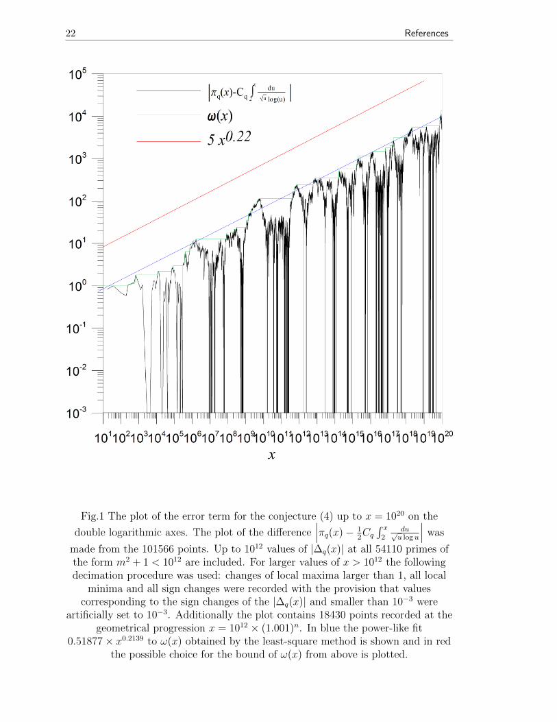
Nothing is known about the error term for the formula (4) (see however [2, 3]), thusthe only way to gain some information and intuition is to appeal to the availablecomputer data. The Figure 1 presents the plot of the difference

|∆q(x)| =∣∣∣∣πq(x)− 1

2Cq

∫ x

2

du√u log u

∣∣∣∣ . (11)

for x ∈ (10, 1020). As it is seen from this plot the graph of the error term is veryerratic, thus the plot of the maximal value of the absolute difference:

ω(x) = max2<t<x

|∆q(t)|, (12)

4 2 The problem of error term

what is a kind of envelope for |∆q(x)|, is also plotted in green in the Figure 1.The error term present in the ordinary Prime Number Theorem (PNT) under

the Riemann Hypothesis is√x log(x):

π(x) = Li(x) +O(√x log(x)). (13)

which can be written in the slightly weaker form

π(x) = Li(x) +O(x12+ε). (14)

TABLE I

x πq(x) Cq√x/ log(x) πq(x)/ eq. (2) formula (4) πq(x)/eq. (4)

106 112 99 1.12713 122 0.91869107 316 269 1.17325 318 0.99440108 841 745 1.12847 855 0.98321109 2378 2095 1.13516 2357 1.008881010 6656 5962 1.11639 6610 1.006961011 18822 17140 1.09815 18787 1.001841012 54110 49684 1.08909 53971 1.002581013 156081 145028 1.07621 156386 0.998051014 456362 425861 1.07162 456405 0.999911015 1339875 1256912 1.06601 1340089 0.999841016 3954181 3726285 1.06116 3955222 0.999741017 11726896 11090399 1.05739 11726340 1.000051018 34900213 33122538 1.05367 34903278 0.999911019 104248948 99229889 1.05058 104251624 0.999971020 312357934 298102838 1.04782 312353427 1.00001

The√x behavior is confirmed by the computer data, see e.g. [32, Table 14, p.

175] or [17, Table 5 and 6], where the difference Li(x)− π(x) has roughly half digitsof the value π(x). Because there are roughly

√x candidates for primes of the form

m2 + 1 up to x it is natural to expect that the error term for (4) will be square rootof the error term for PNT. This heuristic seems to be confirmed by the fact, thatω(x) is well approximated by the power–like error term:

α1xβ1 , α1 = 0.38 . . . , β1 = 0.22 . . . . (15)

and indeed here β1 ≈ 1/4. This function was obtained by fitting the straight line tothe points log(ω(x)) vs log(x) for x > 109 by the least-square method and to boundthe difference ω(x) from above it is sufficient to shift the above curve (15) parallelup to leave the plot of |∆q(x)| below. In the Figure 1 the function 5xβ1 was chosen,but at least for x < 1020 the smaller choice for the constant hidden in the big-O inω(x) = O(xβ1) will also do. These heuristic arguments and computer data lead usto guess the following

5

Conjecture 1:

πq(x) =1

2Cq

∫ x

2

du√u log u

+O(x14+ε). (16)

More stringent error term O(x14

√log(x)) is also a possibility which cannot be ruled

out by available data. Let us notice, that (16) is heuristically supported by therelation (6) and π(

√x) = li(

√x) +O(x1/4). Another support in favor of (16) will be

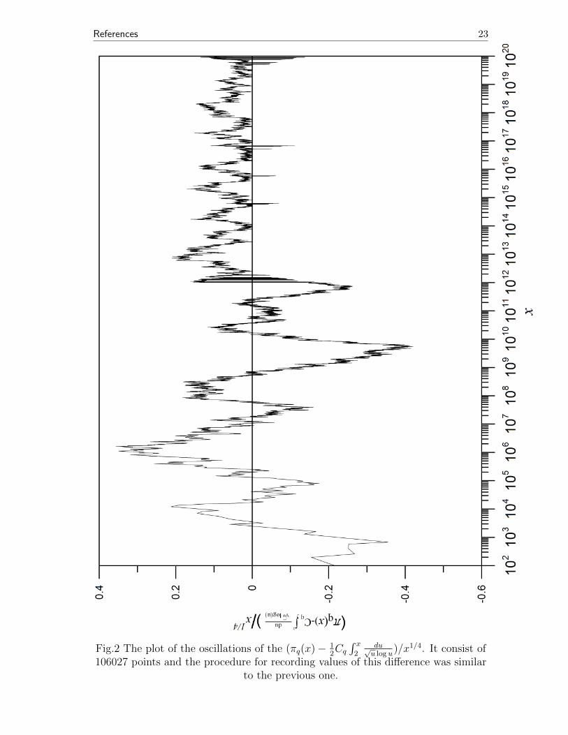
given in Sect.7 (see Fig.8).The difference ∆q(x) fluctuates roughly symmetrically around zero. As the com-

puter check of possible future oscillations theorems we present in the Fig.2 the plotof ∆q(x)/x1/4. The amplitude of this function practically does not change in theinterval (102, 1020) giving support in favor of the error term O(x1/4).

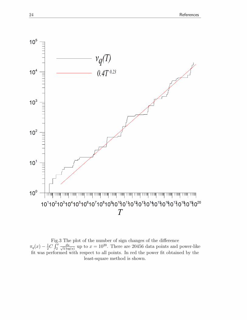
3 An analog of the Skewes number for primes of the formm2 + 1

It turns out that the there is a lot of sign changes of the difference

∆q(x) = πq(x)− 1

2Cq

∫ x

2

du√u log(u)

(17)

in the investigated interval x ∈ (2, 1020). In the generic problem of all prime numbersit was shown by J.E. Littlewood in the 1914 [28] (see also [13]) that the differencebetween the number of primes smaller than x and the logarithmic integral li(x)infinitely often changes the sign. The smallest value xS such that for the first timethe difference ∆(x) = π(x) − li(x) changes the sign is called Skewes number andthe lowest present day known estimate of the Skewes number is around 10316, see[5] and [11]. However in the case of the primes given by the quadratic polynomialm2 + 1 the first sign change of the difference ∆q(x) occurs already at the primeq13 = 2917 = 542 + 1 and there are 20634 such sign changes up to 1020. Let νq(T )denotes the number of sign changes of the function ∆q(x) for x ∈ (2, T ). The Fig.3presents the plot of the function νq(T ) for T < 1020. The fitting of the power–like dependence of νq(T ) on T gives parameters which depend on the number ofdiscarded initial points. For example fitting log(νq(T )) vs log(T ) for T ∈ (107, 1020)gives νq(T ) ∼ T 0.23308 while for T ∈ (1012, 1020) we obtained νq(T ) ∼ T 0.23834, andwe have checked for other intervals of T that the first digits 0.23 persists, thus wewrite:

νq(T ) ≈ α2Tβ2 α2 = 0.38 . . . , β2 = 0.23 . . . (18)

Let us mention that for the case of all primes Knapowski [25] proved that the numberof sign changes of ∆(x) = in the interval (1, T )

ν(T ) ≥ e−35 log log log log T (19)

provided T ≥ exp exp exp exp(35). There is a remarkable coincidence in the valuesof the parameters α and β present in the fits (15) and (18) and when the functionsω(x) and νq(T ) are plotted on the same graph they appear very close to each other,despite the fact that ω(x) and νq(T ) represent quantities at first sight unrelated.

6 4 The analog of the Brun constant

4 The analog of the Brun constant

Because∑∞

n=11n2 = π2/6 <∞ thus the sum of reciprocals of all primes of the form

q = m2 + 1 is trivially convergent:∑q∈Q

1

q=

1

2+

1

5+

1

17+

1

37+

1

101+ . . . <∞ (20)

but the actual numerical value of this sum is unknown [31]. In 1919 Brun [9] hasshown that the sum of reciprocals of all twin primes is finite:

B2 =

(1

3+

1

5

)+

(1

5+

1

7

)+

(1

11+

1

13

)+ . . . <∞. (21)

Numerically B2 = 1.9021605823 . . ., see [29], [8]. It is natural to call the above sum(20) the Brun’s constant for primes of the form q = m2 + 1 and denote it by Bq.From the computer data we can calculate the finite size approximations:

Bq(x) =∑x>q∈Q

1

q. (22)

From the integral test for convergence of the series in the form:

∞∑n=N

f(n) ≤ f(N) +

∫ ∞N

f(u) du. (23)

we have:

Bq =∑x>q∈Q

1

q+∑x<q∈Q

1

q< Bq(x) +

∑n2>x

1

n2< Bq(x) +

1

x+

∫ ∞√x

du

u2= Bq(x) +

1

x+

1√x

(24)Thus from this trivial inequality we can expect for x = 1020 the accuracy of 10 digitsfor Bq. Indeed, from the second column of the Table II we see that the number ofstabilizing digits of Bq(x) is roughly half of the digits of the exponent of x in thefirst column. However, using some heuristics it is possible to obtain from Bq(1020)15 digits of Bq. Namely, we can obtain the analytical formula for dependence ofBq(x) on x. From the equation (4) it follows that the chance to find a prime of the

form m2 + 1 around x is Cq2√x log(x)

,2 thus we can write:

Bq(x) =∑x>q∈Q

1

q≈ Bq(∞)− Cq

2

∫ ∞x

du

u3/2 log(u)(25)

Integrating by parts gives:∫ ∞x

du

u3/2 log(u)= − 2√

x log x+

4√x log2 x

. . .+ (−1)n2n(n− 1)!√x logn x

+ . . . (26)

2 Let us remark, that in the case of all primes π(x) ∼∫ x

2du

log(u) = xlog(x) + . . . as well as of twin

primes π2(x) ∼ C2

∫ x

2du

log2(u)= C2

xlog2(x)

+ . . . the chance to find a prime around x following from

dividing the first terms on r.h.s. by x coincide with integrands on l.h.s, what is not true in thecase of (4), where the factor 1

2 makes the difference.

7

This series is asymptotic one and the condition for the dropped terms is n > 12

log(x)

— the same as threshold (5). But by the change of the variable u = 1/√t it is

possible to express the above integral by the logarithmic integral:∫ b

a

du

u3/2 log(u)= li

(1√b

)− li

(1√a

). (27)

This formula is useless for our purposes, because (9) or (10) is valid for x > 1. Theanalog of (25) for usual Brun’s constant is given by

B2(∞) = B2(x) +2C2

log(x), (28)

where C2 =∏

p>2(1−1

(p−1)2 ) = 0.66016 . . . is the Twins constant.The third column in Table II gives the sample of values

B?q(x) = Bq(x) +Cq2

∫ ∞x

du

u3/2 log(u)(29)

which are supposed to be constant and equal to Bq(∞). As it seen from the TableII indeed with increasing x growing number of digits of the sum (29) is stabilizing.To produce the data for this Table we calculated in PARI the value of Cq withover 30 digits accuracy using the formula (10) from [36]. We calculated the finiteapproximations Bq(x) in DEC Fortran using the quadruple precision (REAL*16)with 33 decimal digits and the Mathematica v.7 was used to calculate integrals (26)with over 30 digits of accuracy.

TABLE II

x Bq(x) B?q(x)

102 0.79575154653780163 0.81798411614326626103 0.81119372199008314 0.81625948818529443104 0.81335296609757082 0.81460891435244917105 0.81432340308206016 0.81465046053349854106 0.81450766696668914 0.81459563341678427107 0.81457232824055968 0.81459653781164721108 0.81458971836435488 0.81459649673657666

......

...1013 0.81459655805079256 0.814596571693407101014 0.81459656768254395 0.814596571704790961015 0.81459657051185242 0.814596571703211291016 0.81459657134862317 0.814596571702922931017 0.81459657159724819 0.814596571702990491018 0.81459657167131276 0.814596571702972371019 0.81459657169347024 0.814596571702976231020 0.81459657170012661 0.81459657170298816

It is seen from the last column that starting with x = 1016 all first 14 digitsremain the same — the change appears at the 14-th place after the dot. In the

8 5 Analog of the conjecture B of Hardy–Littlewood

paper [30] Nicely has performed complicated statistical analysis to get the 95 %confidence interval for the value of B2. In our case it is possible to estimate theerror appearing in (29) by using the form of the function ω(x) given by Conjecture1. Namely, the “density” of the error for the chance Cq

2√x log(x)

to find the prime of

the form m2 + 1 around x is less than O(x−3/4), thus we have:

|Bq(∞)− B?q(x)| = O(x−3/4). (30)

From this we see, that for x = 1020 the value of Bq(∞) lies in the interval ofapproximate length 10−15 around B?q(1020) and we can claim that with 15 digitsaccuracy

Bq(∞) ≡ Bq = 0.81459657170299 . . . . (31)

S. Plouffe has checked using his Symbolic Inverse Calculator (http://pi.lacim.uqam.ca/eng/),that this constant can not be expressed by other mathematical constants [31], thusthe value of Bq could be treated as a new mathematical constant. The compari-son of numbers in the second and third column reveals that addition of the termCq2

∫∞x

duu3/2 log(u)

causes that about 3-4 digits more than in the values of Bq(x) alone

settle down, thus the rate of convergence of B?q(x) is a few orders faster than thatof Bq(x).

The correctness of the choice of 12

in front of the integral in (25) can be checkedby comparing the values of the equation

Bq(x2)− Bq(x1) =Cq2

∫ x2

x1

du

u3/2 log(u)(32)

following from (25) with the actual computer data. For example for x1 = 106 andx2 = 1020 for the l.h.s. of (32) from the computer data we get 0.000177 . . . while ther.h.s. is equal to 0.000176 . . ..

Let us mention that two first primes from Q give contribution 12

+ 15

= 0.7 to Bq,i.e. 86% of the total value 0.8145966 . . .!

We can define the Brun’s measure of the set of numbers S = {a1, a2, . . . , } as thesum

MB(S) =∑i

1

ai(33)

provided it is finite. Thus we can say that the Brun’s measure of the set of twinprimes is 1.9021605823 . . ., while the Brun’s measure of the set Q is MB(Q) =0.8145965717 . . . .

5 Analog of the conjecture B of Hardy–Littlewood

The conjecture B of Hardy–Littlewood [19] says that the number

π(d;x) =∑p<x

p−p′=d

1 =| {p < x : p and p− d are primes} | (34)

of prime pairs p− d, p < x separated by d (d = 2, 4, 6, . . .) is given by

π(d;x) ∼ C2

∏p>2p|d

(p− 1

p− 2

)∫ x

2

dt

log2(t), (35)

9

where

C2 = 2∏p>2

(1− 1

(p− 1)2

)= 1.320323631693739 . . . (36)

is the Twin constant. The integral in (35) again can be expressed by the logarithmicintegral and thus calculated quickly from the series (9) or (10):∫ b

a

dt

log2(t)=

∫ b

a

dt

log(t)+

a

log(a)− b

log(b)= li(b)− li(a) +

a

log(a)− b

log(b)(37)

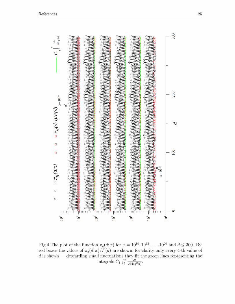
The values of the gaps between primes m2 + 1 and (m − d)2 + 1 grow linearlywith m, but we can formulate an analog of the conjecture B of Hardy–Littlewoodwhen we will focus on the gaps between k′s appearing in 4k2 +1. Thus let us define:

πq(d;x) =| {2k <√x : 4k2 + 1 and 4(k − d)2 + 1 are both primes} | (38)

In contrast to all primes here d = 1, 2, 3, . . .. The Fig. 4 presents the plots of πq(d;x)obtained from our computer data for x = 1010, x = 1012, . . . x = 1020 and d ≤ 300.

There is a heuristic procedure of Bateman and Horn [4] (see also [33, chap. 3])allowing to guess the formula for the number of constellations of primes of differ-ent types. Let f = {f1(x), f2(x), . . . , fl(x)} be the set of distinctive irreduciblepolynomials with integral coefficients and positive leading coefficient such, thatf(x) = f1(x)f2(x) . . . fl(x) has no fixed divisor > 1. Let π(f ;x) denote the numberof positive integers n < x such, that all f1(n), f2(n), . . . , fl(n) are simultaneouslyprimes. Then the Bateman–Horn conjecture reads:

π(f ;x) ∼∏p

1− w(p)p

(1− 1p)l

∫ x

2

du∏li=1 log(fi(u))

, (39)

where w(p) is the number of distinct solutions to f1(u)f2(u) · · · fk(u) ≡ 0 (mod p)with u ∈ {0, 1, . . . , p− 1}. In our case f1(u) = 4u2 + 1, f2(u) = 4(u− d)2 + 1. It iswell known [20, chap. VII] that equation 4u2 + 1 ≡ 0 (mod p) has two solutions forprimes of the form p = 4n + 1 and does not have solutions for primes of the formp = 4n + 3. For the case p = 4n + 1 if p | d then equations f1(u) ≡ 0 (mod p) andf2(u) ≡ 0 (mod p) have the same solutions, thus w(p) = 2. When p - d then thereare two possibilities: w(p) = 3 when f1(u) ≡ 0 (mod p) and f2(u) ≡ 0 (mod p)have one common solution, or w(p) = 4 when f1(u) ≡ 0 (mod p) and f2(u) ≡ 0(mod p) have distinct solutions. The equations f1(u) ≡ 0 (mod p) and f2(u) ≡ 0(mod p) can have one common solution only when p | ±2u? + d, where u? is thesolutions of

4u2 + 1 ≡ 0 (mod p).

The solutions of this equation are of the form (see [20, p.88])

2u1,2 = ±u?, u? =

(p− 1

2

)!

Because the conditions p | ±2u? + d for the case w(p) = 3 can be written as the onecondition p | d2 − 4u? and there is an identity 4u?2 + 1 ≡ 0 (mod p) we can writethe condition for w(p) = 3 simply as p | d2 + 1. Thus we have for p = 4n+ 1

10 5 Analog of the conjecture B of Hardy–Littlewood

w(p) =

4 if p - d, p - d2 + 1

3 if p | d2 + 1

2 if p | d(40)

For p = 2 and for p = 4n+ 3 there are no solutions, i.e. w(p) = 0, hence finallythe product appearing in the Bateman–Horn conjecture takes the form:∏

p

1− w(p)/p

(1− 1/p)2= (41)

4∏

p≡3 (mod 4)

1

(1− 1/p)2

∏p≡1 (mod 4)p-d, p-d2+1

1− 4/p

(1− 1/p)2

∏p≡1 (mod 4)

p|d

1− 2/p

(1− 1/p)2

∏p≡1 (mod 4)p|d2+1

1− 3/p

(1− 1/p)2.

We can get rid of the product over p - d by extending it to the product over allp ≡ 1 (mod 4) and simultaneously by dividing by an appropriate term. Because theconditions p | d and p | d2 + 1 cannot be satisfied simultaneously these additionalfactors can be incorporated into the last two products above. Finally the factordescribing oscillations takes the form (we separated 4 to cancel it later with 4 comingfrom the degrees of f1(u) and f2(u)):∏

p

1− w(p)/p

(1− 1/p)4= 4C1P (d), (42)

where the constant C1:

C1 =∏

p≡3 (mod 4)

p2

(p− 1)2

∏p≡1 (mod 4)

p(p− 4)

(p− 1)2= 0.975245556223143537223292783 . . .

(43)and P (d) denotes the product:

P (d) =∏

p≡1 (mod 4)p|d

p− 2

p− 4

∏p≡1 (mod 4)p|d2+1

p− 3

p− 4. (44)

In above expressions the condition p ≡ 1 (mod 4) means that products are overprimes p ≥ 5, thus all these products are positive. In (44) the conditions p | d andp | d2 + 1 are fulfilled only by finite number of p′s, hence it is obvious that theseproducts are convergent.

Finally we obtain the number of such k < x that both f1(k) = (2k)2 + 1 andf2(k) = (2(k − d))2 + 1 are prime:

π(f1, f2;x) = C1

∏p≡1 (mod 4)

p|d

p− 2

p− 4

∏p≡1 (mod 4)p|d2+1

p− 3

p− 4

∫ x

1

du

log2(2u)(45)

We put here for a while 1 as the lower limit of integration, since k = 1 gives theprime 4 · 12 + 1 = 5 (let us notice, that Ramanujan often did not specify the lower

11

limit of integration, see [6, p.123]). Because we skip 1 in m2 + 1 in manipulationsof integrals below, alternatively we can say that the lower limit of integration is√

5/4 = 1.118033989 . . ..Usually we are interested directly in the number of primes 4k2 + 1 < x and after

the change of the integration variable u =√t/2 we have∫ √b/2

√a/2

du

log2(2u)=

∫ b

a

dt√t log2(t)

(46)

and finally for the quantity πq(d;x) defined in (38) we obtain Conjecture 2:

πq(d;x) = C1

∏p≡1 (mod 4)

p|d

p− 2

p− 4

∏p≡1 (mod 4)p|d2+1

p− 3

p− 4

∫ x

5

dt√t log2(t)

+ error term (47)

We cheated a little here replacing 4 by 5 as the lower limit of integration; better pos-sibility as the lower limit of integration is perhaps the Soldner-Ramanujan constantµ = 1.45136923488338105 . . . defined by li(µ) = 0, see [6, p.123]. Appearing hereintegral by the change of the variable t = u2 can be expressed by the logarithmicintegral: ∫ b

a

dt√t log2(t)

=1

2(li(√b)− li(

√a)) +

√a

log(a)−√b

log(b). (48)

The product P (d) (44) is responsible for characteristic oscillations seen in theFig. 4. The conjecture 2 agrees with the computer data quite well. Instead ofproducing some table to corroborate this statement, we give “visual argument”:in the Fig.4 by the red boxes are plotted values of the quotient πq(d;x)/P (d) forx = 1012, . . . x = 1020 and d ≤ 300. In green are plotted values of the integral∫ x2du/√t log2(t) for the same values of x.

6 Heuristics on the gaps between adjacent k

It is interesting to restrict the analysis from the previous section to the case ofconsecutive values of k giving the prime 4k2 + 1. Let us define the quantity:

h(d;x) = {number of pairs k < k′ = k+d, such that 4k2+1 and 4k′2+1 < x are

consecutive primes of the form m2 + 1} =∑qn<x

qn−qn−1=4d(√qn−1−d)

1. (49)

The Fig. 5 presents the plot of h(d;x) obtained from our computer data forx = 1010, x = 1012, . . . x = 1020. On the semi-logarithmic scale the points displaycharacteristic oscillations around straight lines representing the fits to exponentialdecrease obtained by the least-square method. To describe the oscillations we takethe product P (d) from (44). The Fig.5 presents the corroboration of this mecha-nism of oscillations: dividing the values of h(d, x) by the product P (d) leaves pureexponential decrease — small deviations could be attributed to the fluctuations ofh(d, x) and incorporated into the (unknown) error term.

12 6 Heuristics on the gaps between adjacent k

The Figure 5 suggests the following

Ansatz:h(d, x) = C1P (d)B(x)e−dA(x). (50)

The functions A(x) and B(x), giving the slopes and the intercepts of straight linesseen in the Fig. 5, can be determined by exploiting two selfconsistency conditionsthat h(d, x) has to obey just from the definition. First of all, the number of all gapsbetween k′s is by one smaller than the number of primes of the form 4k2 + 1 smallerthan x:

K(x)∑d=1

h(d, x) = πq(x)− 1, (51)

where K(x) denotes the largest gap between two consecutive k, k′ < x. The secondselfconsistency condition comes from the observation, that the sum of distancesbetween adjacent k is equal to the k producing the largest prime q = 4k2 + 1 ≤ x.For large x we can write:

K(x)∑d=1

h(d, x)d =

√x

2. (52)

The erratic behavior of the product P (d) is an obstacle in calculation of the abovesums (51) and (52). Thus we will replace P (d) by the mean value:

n∑d=1

P (d) = ns+ E(n), (53)

where we assume that the unknown error term E(n) is an increasing function of nwhich grows slower than n:

limn→∞

E(n)

n= 0 (54)

what means that:

s = limn→∞

1

n

n∑d=1

∏p≡1 (mod 4)

p|d

p− 2

p− 4

∏p≡1 (mod 4)p|d2+1

p− 3

p− 4

. (55)

There is known at least one example of the error term which grows slower than n forthe similar problem. Namely, E. Bombieri and H. Davenport [7] have proved thatthe number 1/

∏p>2(1−

1(p−1)2 ) is the arithmetical average for the product

∏p|d

p−1p−2 :

n∑d=1

∏p|d,p>2

p− 1

p− 2=

n∏p>2(1−

1(p−1)2 )

+O(log2(n)). (56)

To get rid of P (d) in (51) and (52) the Abel summation formula can be used inthe form:

n∑i=1

aibi = −n−1∑i=1

S(i)ci + A(n)bn,

13

where S(i) = a1 + . . . ai and ci = bi+1 − bi. Putting here ai = P (i), bi = f(i) andreplacing E(1) < E(2) < . . . < E(n− 1) by larger E(n) we obtain:

n∑l=1

P (l)f(l) = sn−1∑l=1

f(l) +O(f(n)E(n)). (57)

In our case f(l) = C1B(x)e−A(x)l for equation (51) and f(l) = C1lB(x)e−A(x)l forequation (52). From the Fig.5 we see, that h(d, x) decreases exponentially with d andto solve (51) and (52) for e−A(x) and B(x) we have to drop the term O(f(n)E(n)).The sums (51) and (52) are the geometrical and differentiated geometrical seriesrespectively; because h(d, x) decreases exponentially with d we have replaced K(x)in (51) and (52) by ∞ and (51),(52) turn into the equations:

sC1B(x)e−A(x)

1− e−A(x)= πq(x), (58)

sC1B(x)e−A(x)

(1− e−A(x))2=

√x

2. (59)

The solutions for e−A(x) and B(x) of the above equations are:

e−A(x) = 1− 2πq(x)√x

,m (60)

B(x) =2π2

q (x)

sC1

√x(1− 2πq(x)√

x). (61)

Hence we have finally:

h(d;x) =2P (d)π2

q (x)

s√x

(1− 2πq(x)√

x

)d−1+ error term. (62)

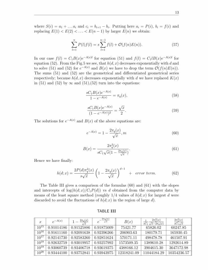
The Table III gives a comparison of the formulas (60) and (61) with the slopesand intercepts of log(h(d;x)/C1P (d)) vs d obtained from the computer data bymeans of the least square method (roughly 1/4 values of h(d;x) for largest d werediscarded to avoid the fluctuations of h(d;x) in the region of large d).

TABLE III

x e−A(x) 1− 2πq(x)√x

e− 2πq(x)√

x B(x) 1sC1

2π2q (x)√

x−2πq(x)2π2q (x)

sC1√x

1015 0.91014186 0.91525886 0.91875009 75421.77 65826.02 60247.851016 0.91611160 0.92091638 0.92396266 206903.63 180179.71 165930.451017 0.92141730 0.92583260 0.92851624 570171.11 498478.78 461507.911018 0.92632759 0.93019957 0.93257992 1573509.35 1389610.28 1292614.891019 0.93060739 0.93406718 0.93619375 4388166.12 3904615.30 3647172.981020 0.93444100 0.93752841 0.93943975 12318241.09 11044184.29 10354236.57

14 6 Heuristics on the gaps between adjacent k

The expression for the mean value s of the product P (d) can be obtained in thefollowing way: Because the pairs of primes of the form (2k)2 + 1 and (2k + 2)2 + 1(Shanks calls in [37] such pairs Gaussian Twins) correspond to d = 1 thus theyare necessarily consecutive (qn, qn+1) and the formula for the number h(1, x) of suchpairs smaller than x obtained from (62) has to be equal to πq(1;x) from (47):

h(1;x) =2π2

q (x)

s√x

= C1

∫ x

5

dt√t log2(t)

(63)

For large x we have πq(x) = Cq√x/ log(x) and∫ x

5

dt√t log2(t)

=1

2li(√x)−

√x

log(x)=

2√x

log2(x)+ . . .

where we have used two first terms of the asymptotic expansion (8) and fortunatelythe term

√x/ log(x) cancels out leaving on both sides of (63) the same dependence

on x and thus we obtain s = C2q /C1:

s = limn→∞

1

n

n∑d=1

∏p≡1 (mod 4)

p|d

p− 2

p− 4

∏p≡1 (mod 4)p|d2+1

p− 3

p− 4

=C2q

C1

. (64)

In the full (mysterious) form it reads:

limn→∞

1

n

n∑d=1

∏p≡1 (mod 4)

p|d

p− 2

p− 4

∏p≡1 (mod 4)p|d2+1

p− 3

p− 4

=

(∏p≥3

(1− (−1)(p−1)/2

p−1

))2

∏p≡3 (mod 4)

p2

(p−1)2∏

p≡1 (mod 4)p(p−4)(p−1)2

(65)We were not able to prove this identity analytically — usual methods of calcu-

lating the sums of arithmetic functions, see e.g. [23, Chap.1], are not applicablehere because P (d) is not a multiplicative function. The computer checking of (65)for large number of terms on the l.h.s. is also difficult because the calculation ofthe average has almost cubic complexity in n (i.e. finding the value of l.h.s. of (65)involves O(n3/ log2(n)) operations). We have calculated the sum of P (d) for d upto 150000 and we obtained

∑150000d=1 P (d)/150000 = 1.93242674 . . ., while the r.h.s.

of (65) is (1.3728134628)2/0.97524552 = 1.93245368, thus the first 5 digits are thesame.

In [37], [14, p. 90], [35] heuristically the formula for h(1;x) was obtained in theform:

h(1, x) = F

√x

log2(x)+ error term (66)

where:

F =π2

2

∏p≡1 (mod 4)

(1− 4

p

)(p+ 1

p− 1

)2

= 1.9504911124462870744465855658 . . . .

(67)

15

In [35] the 50 digits of this constant are given. Therefore we have C1 = F/2, s =2C2

q /F and the combination on the r.h.s of (65) can be transformed to the form:

s =2C2

q

F=

1

4

∏p≡1 (mod 4)

(p− 2)2(p− 1)2

p(p− 4)(p+ 1)2

∏p≡3 (mod 4)

(p+ 1

p− 1

)2

(68)

Finally we state the

Conjecture 3:

h(d, x) =FP (d)π2

q (x)

C2q

√x

(1− 2πq(x)√

x

)d−1+ error term. (69)

For large x we can simplify considerably the above formulas by writing e−A(x) =

1− 2πq(x)√x

as e−A(x) = e− 2πq(x)√

x and B(x) =2π2q (x)

sC1√x, therefore in the limit of large x we

have:

h(d, x) =FP (d)

C2q

√xπ2q (x)e

−d 2πq(x)√x + error term. (70)

The Table III gives the comparison of the quantities e−A(x) and B(x) obtained fromleast-square method applied to log(h(d;x)/C1P (d)) vs d and analytical expressionsfor them.

As a corroboration of the above conjectures we will obtain the formula for themaximal gap K(x) between two consecutive values of k <

√x/2 giving the prime

4k2 + 1. Assuming, that the maximal gap K(x) appears only once we have theequation h(K(x), x) = 1 and putting the Hardy–Littlewood formula for πq(x) in(70) and replacing P (d) by s we obtain:

K(x) ∼ log(x)

2Cq

(1

2log(x) + log(2C2

q )− 2 log(log(x))

)(71)

what for large x goes to the

K(x) ∼ 1

4Cqlog2(x). (72)

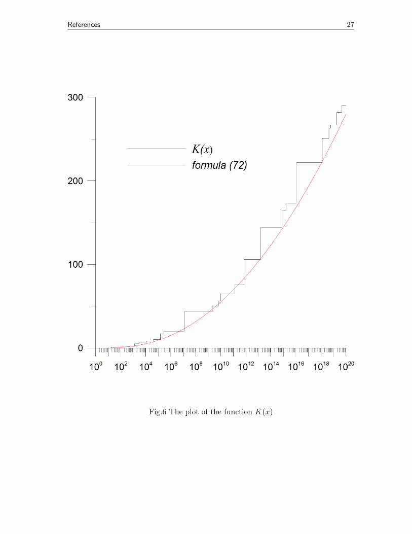
Because for all primes it is widely believed that G(x) ≡ max(pn,pn−1<x)(pn− pn−1) ∼log2(x), we see that K(x) differs from G(x) just by a constant (but here only a frac-tion of k′s are primes!). The largest gap between adjacent k giving 4k2 + 1 < 1020

was 290. The comparison of this formula with computer data is shown in the Figure6. From (72) we deduce the following

Conjecture 4:qn+1 − qn = O(

√qn log2(qn)) (73)

Let us recall that for all primes the Riemann Hypothesis gives pn+1− pn = O(p12+ε

n )for any ε > 0, but in reality gaps between consecutive primes are smaller andthe Cramer conjecture [10] states that pn+1 − pn = O(log2(pn)), see however [16].Because our Conjecture 4 is obtained from the guessed formula for maximal gapbetween k′s we expect (73) to be close to the optimal bound for qn+1 − qn.

16 7 Analog of the Chebyshev’s bias

7 Analog of the Chebyshev’s bias

For ordinary primes the Dirichlet’s Theorem on the primes in arithmetical progres-sions asserts that the number π(x; 4, 1) of primes < x giving 1 as the remainderwhen divided by 4 should be equal to the number π(x; 4, 3) of primes < x giv-ing 3 as the remainder when divided by 4, see e.g. [34]. But the direct inspec-tion shows that for small x there are more primes p ≡ 3 (mod 4) than p ≡ 1(mod 4): π(x; 4, 3) > π(x; 4, 1), what is called Chebyshev’s bias [24]. For the firsttime 1’s takes the lead at p2946 = 26861 — up to this prime 3’s win or there is a tie:π(x; 4, 3) ≥ π(x; 4, 1) for x < 26861. The next time π(x; 4, 3) < π(x; 4, 1) at 616841and in general there is preponderance of primes in the progression 4n + 3. Thesame phenomenon was observed in other arithmetical progressions [17]. Howeverfor the case of number of twins π(2;x) (primes pairs p, p+ 2) and number of cousinsπ(4;x) (primes pairs p, p+ 4) which by the B conjecture of Hardy and Littlewood(35) should be the same π(2;x) ≈ π(4;x), there is no Chebyshev bias at least up to242 ≈ 1.4× 1012: sometimes twins and sometimes cousins take the lead, [41]. In thispaper it was shown numerically that π(2;x) − π(4;x) behaves as the uncorrelatedrandom walk; also the number of returns of this random walk to the origin (thenumber of such x that π(2;x) = π(4;x)) follows the usual square root law

√x [41].

It is in agreement with last sentences of the paper [17] suggesting that there is noChebyshev bias for pairs of primes p, p+ 2k in general.

TABLE IV

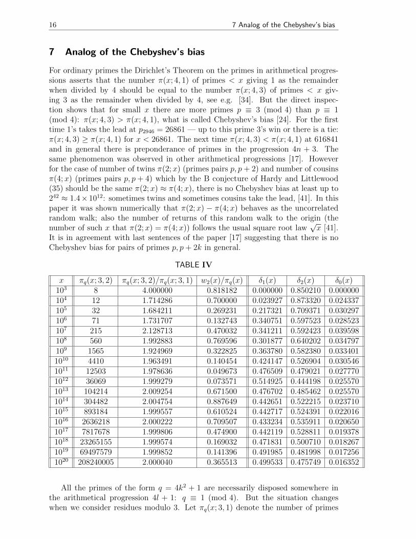
x πq(x; 3, 2) πq(x; 3, 2)/πq(x; 3, 1) w2(x)/πq(x) δ1(x) δ2(x) δ0(x)103 8 4.000000 0.818182 0.000000 0.850210 0.000000104 12 1.714286 0.700000 0.023927 0.873320 0.024337105 32 1.684211 0.269231 0.217321 0.709371 0.030297106 71 1.731707 0.132743 0.340751 0.597523 0.028523107 215 2.128713 0.470032 0.341211 0.592423 0.039598108 560 1.992883 0.769596 0.301877 0.640202 0.034797109 1565 1.924969 0.322825 0.363780 0.582380 0.0334011010 4410 1.963491 0.140454 0.424147 0.526904 0.0305461011 12503 1.978636 0.049673 0.476509 0.479021 0.0277701012 36069 1.999279 0.073571 0.514925 0.444198 0.0255701013 104214 2.009254 0.671500 0.476702 0.485462 0.0255701014 304482 2.004754 0.887649 0.442651 0.522215 0.0237101015 893184 1.999557 0.610524 0.442717 0.524391 0.0220161016 2636218 2.000222 0.709507 0.433234 0.535911 0.0206501017 7817678 1.999806 0.474900 0.442119 0.528811 0.0193781018 23265155 1.999574 0.169032 0.471831 0.500710 0.0182671019 69497579 1.999852 0.141396 0.491985 0.481998 0.0172561020 208240005 2.000040 0.365513 0.499533 0.475749 0.016352

All the primes of the form q = 4k2 + 1 are necessarily disposed somewhere inthe arithmetical progression 4l + 1: q ≡ 1 (mod 4). But the situation changeswhen we consider residues modulo 3. Let πq(x; 3, 1) denote the number of primes

17

q = m2 + 1 < x such that q ≡ 1 (mod 3) and let πq(x; 3, 2) denote the numberof primes q = m2 + 1 < x such that q ≡ 2 (mod 3). The direct inspection of allpossibilities shows that the residue 2 should appear twice as often as the residue 1:

πq(x; 3, 2) ≈ 2πq(x; 3, 1). (74)

It translates into the human 10-base system as the observation, that except for thefirst two cases 2 and 5, the last digit of the primes of the form m2 + 1 can be only1 or 7, see (1). The direct inspection of all 10 possibilities under the assumption ofnormality of digits of k in the base 10 shows, that there are two times more ways ofobtaining 7 than 1.

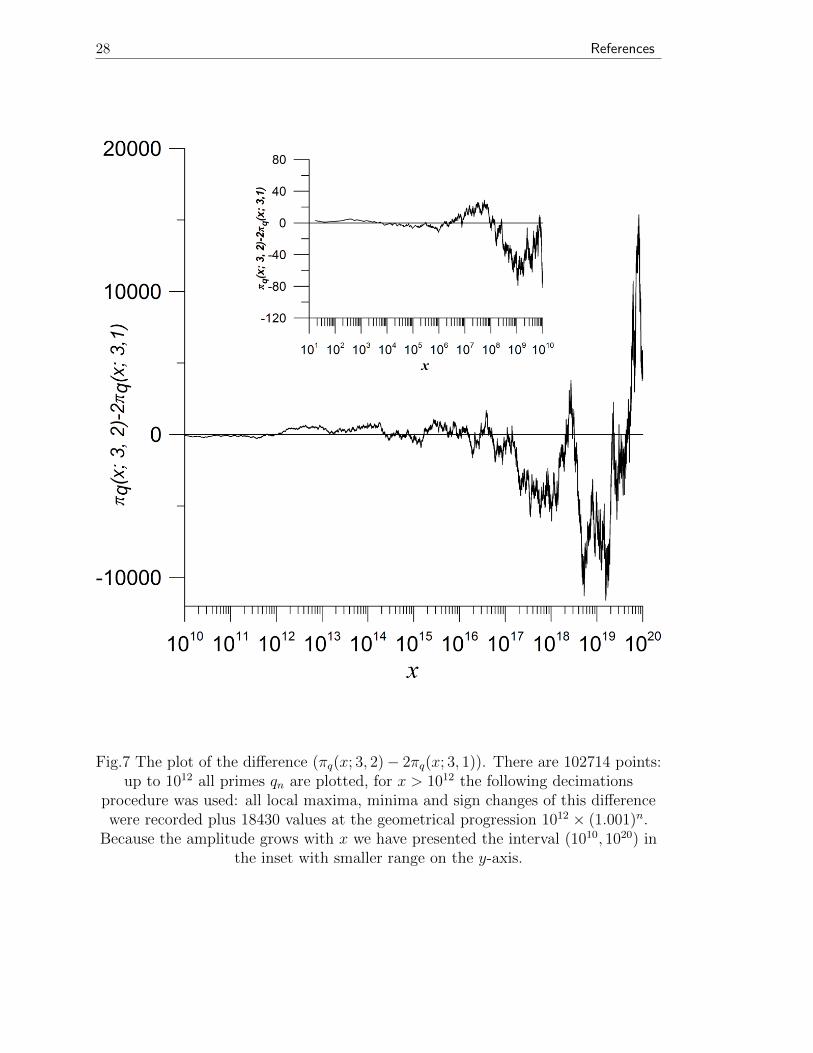
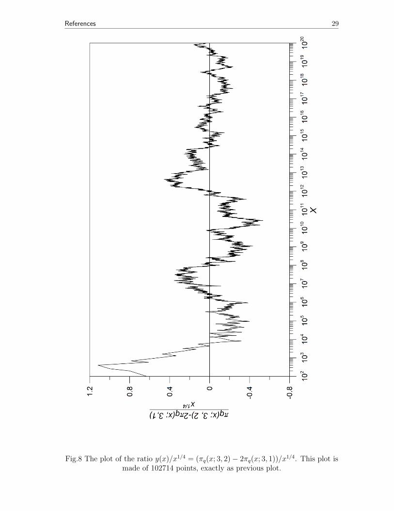
The ratio of the number of those primes p = 4k2 + 1 congruent to 2 modulo 3to those congruent to 1 modulo 3 can give some information about irregularities inthe distribution of primes of the form 4k2 + 1. The Table IV shows the values ofthe ratio πq(x; 3, 2)/πq(x; 3, 1) for x = 103, . . . 1020. As it is seen from this Tableafter the initial transient interval below 107 this ratio begins to oscillate around thepredicted value 2. Initially πq(x; 3, 2) > 2πq(x; 3, 1) and for the first time πq(x; 3, 2) <2πq(x; 3, 1) at q17 = 4 ·422+1 = 7057, i.e. at the 17-th prime of the form q = m2+1.Recently A. Granville and G. Martin [17] have discussed several examples of ”primeraces”. Primes of the form q = 4k2 + 1 provide another example of such a race.Namely we will say that two wins at a given x if πq(x; 3, 2) > 2πq(x; 3, 1) and letw2(x) denote the number of those primes q = 4k2 +1 < x that residue two wins overresidue one. In the third column of the Table IV the ratio w2(x)/πq(x) is shown.As it is seen from this sample of numbers there are large fluctuations of the ratiow2(x)/πq(x). The Fig.7 shows the plot of πq(x; 3, 2) − 2πq(x; 3, 1) up to x = 1020.This plot can be interpreted as a kind of one dimensional random walk: let y(x)denote the displacement of the walker at the “time” x, which plays the role of thetime. If for a given q ∈ Q we find that q ≡ 1 (mod 3) the random walker performsstep down of length 2 and if q ≡ 2 (mod 3) the random walker performs step upof length 1 at the moment x = q. In other moments of time x the walker simplydoes not move. Thus we have y(x) = πq(x; 3, 2) − 2πq(x; 3, 1). This plot resemblesusual random walk, there were 21349 returns to the origin of this random walk upto 1020. There are large regions that y(x) > 0 as well as y(x) < 0 suggesting thatthere is no Chebyshev bias in the distribution of primes qn. In the Fig.8 the plot ofy(x)/x1/4 = (πq(x; 3, 2) − 2πq(x; 3, 1))/x1/4 is shown. The amplitude of oscillationsin this plot seems to be constant over the interval (103, 1020) and contained in thevery short interval (−1

2, 1

2). Dividing (πq(x; 3, 2) − 2πq(x; 3, 1)) by xα results in

amplitudes going to zero when α > 14

and increasing when α < 14. It is another

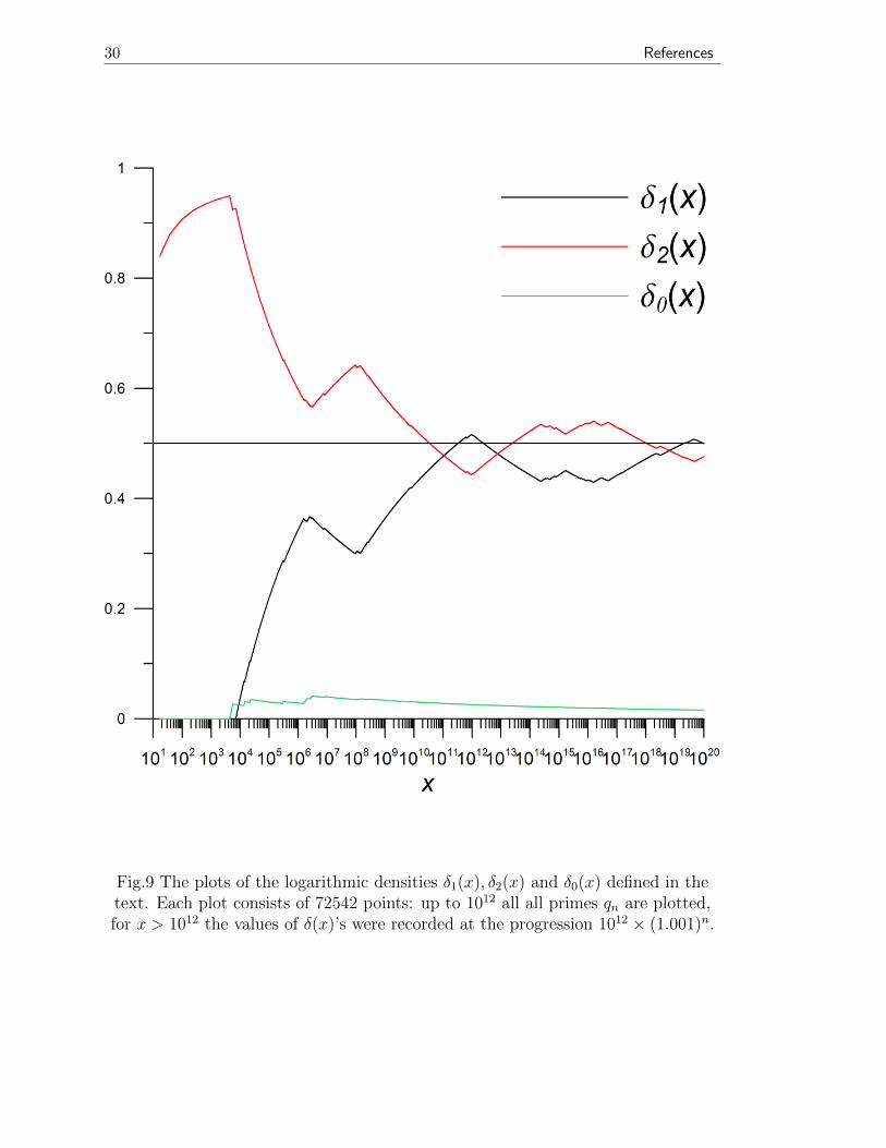
argument in favor of the error term conjectured in the Sect. 2. There are probablylogarithmic factors present, like for the usual Chebyshev bias, see Fig. 6 in [17], butwe are not able to separate it. The amplitude of oscillations of y(x)/x1/4 is verysmall, less than 0.5 and roughly half of the plot in Fig.8 is greater than zero androughly half is below line zero. In [34] it was proposed to use the logarithmic densityto measure the Chebyshev bias. Here we will define these densities for primes fromQ as follows:

δ1 = limx→∞

1

log(x)

∑2≤n<x

2πq(n;3,1)>πq(n;3,2)

1

n(75)

18 7 Analog of the Chebyshev’s bias

δ2 = limx→∞

1

log(x)

∑2≤n<x

2πq(n;3,1)<πq(n;3,2)

1

n(76)

δ0 = limx→∞

1

log(x)

∑2≤n<x

2πq(n;3,1)=πq(n;3,2)

1

n(77)

We do not have at our disposal any formulas like those in [34] and we have to turnto the brute force numerical calculation of finite size approximations δ1(x), δ2(x) andδ0(x) given by expressions (75)— (77) without limit operation limx→∞. The resultsare presented in the 5-th, 6-th and 7-th column of the Table IV and in Figure 9. Upto x = 231 the data for the Table IV and Figure 9 was obtained by direct summing ofthe harmonic sums, for x > 231 ≈ 2.15× 109 the incredible accurate approximation[12], [21, pp. 76-78]

m∑k=n

1

k= log

(m+

1

2

)− log

(n− 1

2

)+O

(1

n2

)(78)

was used, thus the error of each summand was smaller than 10−19, and as there wereO(108) terms, in the worst case of adding up all roundoffs we expect the total errorto be smaller than 10−10. To calculate the harmonic series up to x = 1020 directlyby adding all numbers 1/n would take a few thousands years of CPU time, but it isin general impossible using standard programming languages as the loop can haveonly integer counter and on 64 bit processors the largest integer is 263 ≈ 9.22×1018.

For all primes Chebyshev conjectured that

limx→∞

∑p>2

(−1)p−12 e−p/x = −∞ (79)

It was proved by Hardy and Littlewood [18] and Landau [27], [26] that (79) is trueif and only if the L-function

L(s, χ1) =∞∑n=0

(−1)n

(2n+ 1)s(80)

does not have nontrivial zeros outside the critical line <(s) = 12. Here we formulate

the analogous function for the case of primes from Q:

F (x) =∑q∈Q

cqe−q/x (81)

where

cq =

{2 when q mod 3 = 1−1 when q mod 3 = 2

(82)

We made the plot of F (x) and in contrast to (79) this function seems to not possessa limit when x→∞. Because values of F (x) sometimes are close to zero calculatingthe sum (81) on the computer we have stopped summation at such q′ that∣∣∣∣∣ cq′e

−q′/x∑q′

q=2 cqe−q/x

∣∣∣∣∣ < 10−8, (83)

References 19

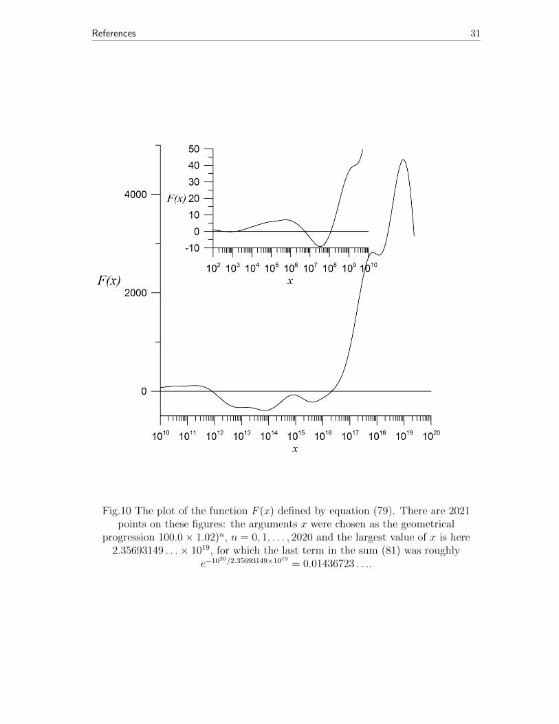
thus we have used relative error. Using such a condition (83) for terminating thesum in (81) is necessary as F (x) sometimes crosses zero and using absolute error canbe misleading at small values of F (x). The last 43 points in the Fig. 10 were notfulfilling the requirement (83) as all primes q = m2 + 1 generated were exhausted,but as it is seen in the plot of F (x) in Fig. 10 values of the function F (x) are wellabove 1000 for x > 1017.

The numbers presented in the Table IV and plots in the Figures 8, 9 and 10allow us to formulate the

Conjecture 5: There is no Chebyshev bias for primes of the form m2 + 1:δ1 = δ2 = 1

2, δ0 = 0

It is the last conjecture formulated in this paper.

Acknowledgment: I would like to thank Prof. Bernd Fischer for suggestingme in December of 1996 the search for primes of the form m2 + 1. I thank Dr JerzyCis lo, Prof. Andrew Granville and Prof. W ladys law Narkiewicz for many commentsand remarks.

References

[1] M. Abramowitz and I. A. Stegun. Handbook of Mathematical Functions withFormulas, Graphs, and Mathematical Tables. Dover, New York, ninth doverprinting, tenth gpo printing edition, 1964.

[2] S. Baier and L. Zhao. On primes in quadratic progressions, 2007. http://xxx.lanl.gov/abs/math/0701577.

[3] S. Baier and L. Zhao. Primes in quadratic progressions on average. Mathema-tische Annalen, 338(4):963–982, 2007.

[4] P. Bateman and R. A. Horn. heuristic asymptotic formula concerning thedistribution of prime numbers. Mathematics of Computation, 16:363–367, 1962.

[5] C. Bays and R. Hudson. A new bound for the smallest x withπ(x) − Li(x). Mathematics of Computation, 69:1285–1296, 2000. availablefrom http://www.ams.org/mcom/2000-69-231/S0025-5718-99-01104-7/

S0025-5718-99-01104-7.pdf.

[6] B. C. Berndt. Ramanujan’s Notebooks, Part IV. Springer Verlag, 1994.

[7] E. Bombieri and H. Davenport. Small differences between prime numbers. Proc.Royal Soc., A293:1–18, 1966.

[8] R. Brent. Irregularities in the distribution of primes and twin primes. Mathe-matics of Computation, 29:43–56, 1975. available from http://wwwmaths.anu.

edu.au/~brent/pd/rpb024.pdf.

[9] V. Brun. La serie 1/5 + 1/7 +... est convergente ou finie. Bull. Sci.Math.,43:124–128, 1919.

20 References

[10] H. Cramer. On the order of magnitude of difference between consecutive primenumbers. Acta Arith., II:23–46, 1937.

[11] P. Demichel. The prime counting function and related subjects. , available fromhttp://www.mybloop.com/dmlpat/maths/li_crossover_pi.pdf.

[12] D. W. DeTemple. A quicker convergence to Euler’s constant. The AmericanMathematical Monthly, 100(5):468–470, 1993.

[13] W. Ellison and F. Ellison. Prime Numbers. John Wiley and Son, 1985.

[14] S. Finch. Mathematical Constants. Cambridge University Press, 2003.

[15] J. Friedlander and H. Iwaniec. The polynomial x2 + y4 captures its primes.Ann. of Math., 148:945–1040, 1998.

[16] A. Granville. Harald Cramer and the distribution of prime numbers. Scan-danavian Actuarial J., 1:12–28, 1995.

[17] A. Granville and G. Martin. Prime number races. American MathematicalMonthly, 113:1–33, 2006.

[18] G. H. Hardy and J. E. Littlewood. Contributions to the theory of the Riemannzeta function and the theory of prime distribution. Acta Mathematica, 41:119–196, 1918.

[19] G. H. Hardy and J. E. Littlewood. Some problems of ‘Partitio Numerorum’ III:On the expression of a number as a sum of primes. Acta Mathematica, 44:1–70,1922.

[20] G. H. Hardy and E. M. Wright. An Introduction to the Theory of Numbers.Oxford Science Publications, 1980.

[21] J. Havil. Gamma: Exploring Euler’s Constant. Princeton University Press,Princeton, NJ, 2003.

[22] H. Iwaniec. Almost-primes represented by quadratic polynomials. Invent.Math.,47:171188, 1978.

[23] H. Iwaniec and E. Kowalski. Analytic Number Theory, volume 53 of ColloquiumPublications. Colloquium Publications, Amer. Math. Soc., 2004.

[24] J. Kaczorowski. The boundary values of generalized Dirichlet series and aproblem of Chebyshev. Asterisque, 209:227–235, 1992.

[25] S. Knapowski. On sign changes of the difference π(x)−Li(x). Acta Arithmetica,VII:106–119, 1962.

[26] E. Landau. ber einen Satz von Tschebyschef. Math. Zeitschr., 47:213–219,1918.

[27] E. Landau. ber einige ltere Vermutungen und Behauptungen in derPrimzahltheorie. Math. Zeitschr., 47:1–24, 1918.

References 21

[28] J. Littlewood. Sur la distribution des nombres premieres. Comptes Rendus,158:1969–1872, 1914.

[29] T. Nicely. Enumeration to 1.6 × 1015 of the twin primes and brun’s constant.http://www.trnicely.net/twins/twins2.html.

[30] T. Nicely. A table of prime counts pi(x) to 5 × 1015. http://www.trnicely.

net/pi/tabpi.html.

[31] S. Plouffe. e-mail from 28-th July 2008.

[32] P. Ribenboim. The Little Book of Big Primes. 2ed., Springer, 2004.

[33] H. Riesel. Prime Numbers and Computer Methods for Factorization. BirkhuserBoston, 1994.

[34] M. Rubinstein and P. Sarnak. Chebyshevs bias. Experimental Mathematics,3:173–197, 1994.

[35] P. Sebah and X. Gourdon. Constants from number theory. availablefrom http://numbers.computation.free.fr/Constants/Miscellaneous/

constantsNumTheory.ps.

[36] D. Shanks. A sieve method for factoring numbers of the form n2 + 1. Mathe-matical Tables and Other Aids to Computation, 13(66):78–86, 1959.

[37] D. Shanks. A note on gaussian twin primes. Math. Comp, 14:201–203, 1960.

[38] D. Shanks. On the conjecture of Hardy and Littlewood concerning the numberof primes of the form n2 + a. Math. Comp, 14:321–332, 1960.

[39] The PARI Group, Bordeaux. PARI/GP, version 2.3.2, 2008. available fromhttp://pari.math.u-bordeaux.fr/.

[40] M. Wolf. On the pairs of primes of the form (p, 4p2 + 1), in preparation.

[41] M. Wolf. Random walk on the prime numbers. Physica A, 250(1-4):335–344,Feb 1998.

[42] M. Wunderlich. On the Gaussian primes on the line Im(x)= 1. Math. Comp.,27:399–400, 1973.

22 References

Fig.1 The plot of the error term for the conjecture (4) up to x = 1020 on the

double logarithmic axes. The plot of the difference∣∣∣πq(x)− 1

2Cq∫ x2

du√u log u

∣∣∣ was

made from the 101566 points. Up to 1012 values of |∆q(x)| at all 54110 primes ofthe form m2 + 1 < 1012 are included. For larger values of x > 1012 the followingdecimation procedure was used: changes of local maxima larger than 1, all local

minima and all sign changes were recorded with the provision that valuescorresponding to the sign changes of the |∆q(x)| and smaller than 10−3 were

artificially set to 10−3. Additionally the plot contains 18430 points recorded at thegeometrical progression x = 1012 × (1.001)n. In blue the power-like fit

0.51877× x0.2139 to ω(x) obtained by the least-square method is shown and in redthe possible choice for the bound of ω(x) from above is plotted.

References 23

Fig.2 The plot of the oscillations of the (πq(x)− 12Cq∫ x2

du√u log u

)/x1/4. It consist of106027 points and the procedure for recording values of this difference was similar

to the previous one.

24 References

Fig.3 The plot of the number of sign changes of the differenceπq(x)− 1

2C∫ x2

du√u log(u)

up to x = 1020. There are 20456 data points and power-like

fit was performed with respect to all points. In red the power fit obtained by theleast-square method is shown.

References 25

Fig.4 The plot of the function πq(d;x) for x = 1010, 1012, . . . , 1020 and d ≤ 300. Byred boxes the values of πq(d;x)/P (d) are shown; for clarity only every 4-th value ofd is shown — descarding small fluctuations they fit the green lines representing the

integrals C1

∫ x5

dt√t log2(t)

.

26 References

Fig.5 The plot of the histogram h(d;x) for x = 1010, 1012, . . . , 1020. . By red boxesthe values of h(x, d)/P (d) are shown; for clarity only every 4-th red box is shown.

They are supposed to lie along the green lines representing the plots of theπ2q (x)

s√x

(1− 2πq(x)√

x

)d−1.

References 27

Fig.6 The plot of the function K(x)

28 References

Fig.7 The plot of the difference (πq(x; 3, 2)− 2πq(x; 3, 1)). There are 102714 points:up to 1012 all primes qn are plotted, for x > 1012 the following decimations

procedure was used: all local maxima, minima and sign changes of this differencewere recorded plus 18430 values at the geometrical progression 1012 × (1.001)n.

Because the amplitude grows with x we have presented the interval (1010, 1020) inthe inset with smaller range on the y-axis.

References 29

Fig.8 The plot of the ratio y(x)/x1/4 = (πq(x; 3, 2)− 2πq(x; 3, 1))/x1/4. This plot ismade of 102714 points, exactly as previous plot.

30 References

Fig.9 The plots of the logarithmic densities δ1(x), δ2(x) and δ0(x) defined in thetext. Each plot consists of 72542 points: up to 1012 all all primes qn are plotted,for x > 1012 the values of δ(x)’s were recorded at the progression 1012 × (1.001)n.

References 31

Fig.10 The plot of the function F (x) defined by equation (79). There are 2021points on these figures: the arguments x were chosen as the geometrical

progression 100.0× 1.02)n, n = 0, 1, . . . , 2020 and the largest value of x is here2.35693149 . . .× 1019, for which the last term in the sum (81) was roughly

e−1020/2.35693149×1019 = 0.01436723 . . ..