Sea Surface Multipath Effects on Ship Radar Radiated Power
70
Naval Research Laboratory Washington, DC 20375-5320 NRL/MR/8124--98-8178 Sea Surface Multipath Effects on Ship Radar Radiated Power Determination WENDY L. LIPPINCOTT Advanced Systems Technology Branch Space Systems Development Department June 30,1998 19980717 021 Approved for public release; distribution is unlimited.
Transcript of Sea Surface Multipath Effects on Ship Radar Radiated Power

Naval Research Laboratory Washington, DC 20375-5320
NRL/MR/8124--98-8178
Sea Surface Multipath Effects on Ship Radar Radiated Power Determination
WENDY L. LIPPINCOTT
Advanced Systems Technology Branch Space Systems Development Department
June 30,1998
19980717 021
Approved for public release; distribution is unlimited.

REPRODUCTION QUALITY NOTICE
This document is the best quality available. The copy furnished to DTIC contained pages that may have the following quality problems:
• Pages smaller or larger than normal.
• Pages with background color or light colored printing.
• Pages with small type or poor printing; and or
• Pages with continuous tone material or color photographs.
Due to various output media available these conditions may or may not cause poor legibility in the microfiche or hardcopy output you receive.
b^J If this block is checked, the copy furnished to DTIC contained pages with color printing, that when reproduced in Black and White, may change detail of the original copy.

REPORT DOCUMENTATION PAGE Form Approved OMB No. 0704-0188
Public reporting burden for this collection of information is estimated to average 1 hour per response, including the time for reviewing instructions, searching existing data sources, gathering and maintaining the data needed, and completing and reviewing the collection of information. Send comments regarding this burden estimate or any other aspect of this collection of information, including suggestions for reducing this burden, to Washington Headquarters Services, Directorate for Information Operations and Reports, 1215 Jefferson Davis Highway, Suite 1204, Arlington, VA22202-4302, and to the Office of Management and Budget, Paperwork Reduction Project (0704-0188), Washington, DC 20503.
1. AGENCY USE ONLY (Leave BlanQ 2. REPORT DATE
June 30, 1998
3. REPORT TYPE AND DATES COVERED
Final Report
4. TITLE AND SUBTITLE
Sea Surface Multipath Effects on Ship Radar Radiated Power Determination
5. FUNDING NUMBERS
6. AUTHOR(S)
Wendy L. Lippincott
7. PERFORMING ORGANIZATION NAME(S) AND ADDRESS(ES)
Naval Research Laboratory Washington, DC 20375-5320
8. PERFORMING ORGANIZATION REPORT NUMBER
NRL/MR/8124--98-8178
9. SPONSORING/MONITORING AGENCY NAME(S) AND ADDRESS(ES)
SPAWAR SAP/FMBMB (AFOY) Washington, DC 200500-6335
10. SPONSORING/MONITORING AGENCY REPORT NUMBER
11. SUPPLEMENTARY NOTES
12a. DISTRIBUTION/AVAILABILITY STATEMENT
Approved for public release; distribution unlimited.
12b. DISTRIBUTION CODE
13. ABSTRACT {Maximum 200 words)
This report presents an overview of sea surface multipath effects on accurate determination of effective radiated power (ERP)
data from ship navigation radars over a 5-20 nautical mile region. The intent is to characterize the various multipath phenomena
affecting signal characterization. Data was collected for several hundred ship radars, and various refractivity and multipath programs
utilized to model the effect.
14. SUBJECT TERMS
Multipath Radar Sea-surface multipath ERP Radiated power Navigation radar
15. NUMBER OF PAGES
69
16. PRICE CODE
17. SECURITY CLASSIFICATION OF REPORT
UNCLASSIFIED
18. SECURITY CLASSIFICATION OF THIS PAGE
UNCLASSIFIED
19. SECURITY CLASSIFICATION OF ABSTRACT
UNCLASSIFIED
20. LIMITATION OF ABSTRACT
UL
NSN 7540-01-280-5500 Standard Form 298 (Rev. 2-89) Prescribed by ANSI Std 239-18 298-102

TABLE OF CONTENTS
SECTION PAGE
I. INTRODUCTION
II. COMPUTER CODES FOR MULTIPATH MODELING
III. ERP CALCULATIONS
IV. STATIC MULTIPATH EFFECTS
V. UPPER AIR SOUNDINGS AND CORRELATION TO MODELING
1
3
5
10
15
VI. RAIN ATTENUATION MODELING
VII. ERP DATA COLLECTION AND VALIDATION
VIII. SUMMARY
ACKNOWLEDGMENTS
REFERENCES
24
26
32
32
33
Appendix A. Appendix B. Appendix C.
Appendix D. Appendix E. Appendix F. Appendix G.
Appendix H. Appendix I.
Overview of Ducting Navigation Radars Effective Earth Radius, Refractivity, and Altitude from Barometric Readings Wind Speed versus Wave Height EREPS Modeling Results Codes for Multipath Modeling ERP Determination from Ship Data: Sample Plots Upper Air Soundings Weather Sources
36 39 40
43 44 49 50
54 65
in

Sea Surface Multipath Effects on Ship Radar Radiated Power Determination
I. INTRODUCTION
One of the factors in defining a ship's radar is effective radiated power (ERP). Knowing the ERP of a radar along with scan rate, frequency, and beam width characterizes the radar in terms of type, size, and transmitter power. This information can be useful in quantifying ship traffic in port areas.
To obtain accurate ERP data from ship radars over a short 5-20 nautical mile link, multipath effects must be accounted for. Multipath effects have been studied extensively [1-12]. Sea surface multipath results from two different phenomena - optical interference and ducting. Optical interference occurs when the radar signal from the ship to the station travels in both a direct path and a path reflecting off the water (Fig. 1). The signals from the two paths combine in and out of phase depending on the distances and radar frequency and cause the signal strength to vary. The reflected signal can also be affected by sea state and the presence of ship wakes and other sea obstructions (buoys and other ships).
Fig. 1 Optical Interference
Multipath from optical interference can be specular or diffuse. The specular component is coherent with respect to the direct signal, and is well- defined in terms of amplitude, phase, and incident direction. The diffuse component has a random nature, and arises from scattering sources from many directions [13]. Generally, specular multipath is modeled with the diffuse component added in through a reflection coefficient. The diffuse component becomes stronger at low grazing angles and for high sea states. With diffuse scattering, the deep nulls associated with optical interference effects are smoothed out.
The second multipath phenomenon is ducting. A duct is a layer of air with different properties than its surroundings which acts as a waveguide to trap electromagnetic energy. These refractive gradients in the atmosphere can cause over-the-horizon fields to be tens of decibels higher than expected. Refractivity profiles can be measured by radiosondes to indicate the presence of ducts. This technique is not suitable in many situations since the radiosonde emits high
Manuscript approved April 24,1998.

power and must be flown at a range of heights. Also, the radiosonde only measures the refractivity profile directly above the receiving station, whereas, depending on the transmitter location, it may be the profile several kilometers away which is affecting the signal. Refractivity profiles change on a hourly basis, so obtaining adequate refractivity data to predict ducting can be unfeasible for other than short term experiments.
Ducting can occur with various meteorological conditions. Evaporation ducts, caused by the rapid decrease in humidity with increasing altitude just above the ocean's surface, occur with the base of the duct at the sea surface. Surface-based ducts generally occur at higher heights than evaporation ducts. They are caused by temperature and humidity inversions when a warm dry air mass moves over a cool, moist air mass. [15] Ducting effects are more prominent at longer ranges and allow reception of RF signals at much longer ranges than would normally occur. Fig. 2 shows a schematic of ducting. Appendix A gives more detailed information about the ducting phenomena. Appendix B summarizes common characteristics of navigation radars.
Fig. 2 Ducting
Various methods can be used to counteract the effects of multipath. For communication links, the use of spatial and frequency diversity has been used. Kuhnert and Gelerman [14] describe the use of two frequencies and two heights
An adaptive equalizer was used. on a receiving tower to counteract ducting
This study is broken into six sections. The first describes various computer codes used for analyzing multipath. The second describes details of the ERP determination process. In the third section, a fixed sea-surface link is used to analyze sea-surface multipath, including tidal effects. The fourth section describes upper air soundings performed over the Chesapeake Bay. The sounding data provides refractivity profiles that are used as input to a computer code to further analyze multipath and particularly ducting effects on ERP data collection. The fifth section describes models to predict radio frequency (rf) attenuation due to rain. Along with multipath effects, rain attenuation can also affect accurate ERP determination. The last section gives results of the ERP data collection experiment which involved taking data on several hundred ships. Several techniques are used to estimate the accuracy of the data.

II. COMPUTER CODES FOR MULTIPATH MODELING
Several computer codes are available to model sea surface multipath effects. The EREPS (Engineer's Refractive Effects Prediction System) code [15,16] models optical interference, diffraction, tropospheric scatter, refraction, evaporation and surface-based ducting, and water vapor absorption under horizontally homogeneous atmospheric conditions. The refractivity profile of the atmosphere is approximated by the use of an effective earth radius (Appendix C). Wave height is modeled as a function of wind speed as described in Appendix D. Figure 3 shows a sample output of the EREPS code, showing a comparison of propagation loss versus range with and without a 13 m high evaporation duct. In this case, the presence of a duct greatly decreases the propagation loss for distances beyond 20 nm.
80
100
5 120 CO CO o 3 140 - c o & 160 CO Q.
Q.
-i—n—|—'—i—r—i—|—i—n—i—[—l—n—i—r-1—*~'—"H—'—r~'—f-!—r~l—■—r~T—r
no duct 13 m evaporation duct
180 -
200 -
220 -
0 10 15 20 25 30 35 40
Range, nautical miles Fig. 3 Propagation loss versus range for radar at 9400 MHz with and without evaporation duct (EREPS code, Wind speed = 10 knots, Transmitter height = 60 ft, Receiver height =180 ft, no ducting, omni transmitter)
Several EREPS runs comparing results with varying wind speed, ducting conditions, receiver/transmitter heights, and frequencies are presented in Appendix E. Runs were also done using spatial diversity (where signals from two receiver heights are combined). The multipath lobing dramatically decreases for this case. It was found that the EREPS code is only good for coarse predictions because the refractivity profile is assumed to be linear. The duct features are approximate as well.

The Northam Multipath code [17,18] models multipath effects for microwave radar signals for low grazing angle, forward scatter, over-water multipath. Northam characterizes over-water multipath as having both specular and diffuse components. These components are influenced by sea state, reflectivity of the water, radar frequency, and polarization. In Northam's model, the sea-state is represented by the root mean square (RMS) surface displacement above the mean. The specular component is treated as a deterministic component, with parameters unknown to the tracking system. The diffuse component is treated as stochastic. This code was specifically designed to model multipath effects on pulse structure. It is a Fortran code which currently runs on a Macintosh computer.
The Radio Physical Optics (RPO) [19] code is similar to EREPS but includes the use of refractivity profiles. It can calculate range-dependent electromagnetic (EM) system propagation loss for a heterogeneous atmosphere. The radio-frequency index-of-refraction can be varied both vertically and horizontally. This code was developed by the Propagation Division at NOSC in San Diego, California, which has developed several other propagation codes and releases them over the Internet. The RPO code was found to be useful for much of the modeling required in this report. Its main limitation was in needing large amounts of refractivity data, which change on an hourly basis and are difficult to obtain. In our case, using one refractivity profile for the entire 9 nm over- water link did not provide exact predictions for link performance, although relative performance estimates could be obtained and are valuable for analyzing the link data. Walters, et. al., [20] has used the RPO code for validating radar performance using refractivity data from a tethered radiosonde with some success.
The Advanced Propagation Model (APM 1.0) from NOSC is a hybrid model that consists of four sub-models: flat earth, ray optics, extended optics, and split-step parabolic equation (PE). APM effectively merges both the Radio Physical Optics (RPO) model and the Terrain Parabolic Equation Model (TPEM). The result is a new and improved EM propagation model that can model range-dependent refractivity environments, variable terrain, range- varying dielectric ground constants for finite conductivity and vertical polarization calculations, troposcatter, and gaseous absorption. This code has only recently become available for public distribution and was not used in this study.
A listing of other computer codes for multipath modeling is given in Appendix F. Results of computer modeling will be compared to experimental data in the following sections.

III. ERP Calculations
The ERP data collected in this report was taken at the Chesapeake Bay Detachment (CBD) of NRL at Chesapeake Beach, Maryland [21]. Collection antennas are set 118 ft. above the water level on a cliff overlooking the bay. The x-band (8-12 GHz) and s-band (2-4 GHz) antennas are omnidirectional bicones that are shielded in the rear by an enclosure, giving them a pattern that is relatively flat to +/- 60°. This type of pattern enables the signal amplitudes to be calculated with just one value for the antenna gain, while rejecting signals in other directions. A receiver system attached to the antennas allowed range, frequency, scan rate, and illumination time (pulse width) data to be taken along with signal amplitude.
The space path loss, L, of power of a radio wave in space is [22]:
2 L =
V * J V c J where
R = range X,= wavelength.
For radar signals from ships, optical interference from the sea surface creates a multipath effect, where the signal strength varies as the range is varied. Figure 1 shows the case where a signal from a ship travels directly to the receiver and also takes a path which bounces off the water. The signals from the two paths combine in and out of phase depending on the distances and frequency, so the signal strength will vary as the ship moves, as the tide varies, and as the sea state changes. This phenomenon is also affected by the presence of ship wakes and other sea obstructions (buoys and other ships). Figure 4 shows an example of interference effects for an over-water link and two receiver heights using the EREPS code. As the receiver (or transmitter) height changes, the interference pattern shifts so that the peaks and nulls occur at shifted locations.

80 I—i—i—r—i—r-r
CD ■o
CO tfl O _l
o
p a.
1—i—i—|—i—i—i—i—|—i—n—1~-|—i—i—i—i—|—r—l—i—r
■180ft. receiver heiqht ■150ft. receiver height
0 35 40 5 10 15 20 25 30
Range, nautical miles Fig. 4 Propagation Loss versus range for over-water link at 9400 MHz with varying receiver heights (EREPS code, Wind speed = 10 knots, Transmitter height = 60 ft, no ducting, omni transmitter)
Figure 5 shows an example of wind speed effects for an over-water link using the EREPS code. Wave height is modeled as a function of wind speed in the EREPS code (Appendix D). High winds correlate to large wave heights, which mute out the interference pattern and reduce the null depth. The peaks of the signal are also lowered. At 5 nm, the peak of the signal is lowered by 1 dB with a 15 knot wind (2.5 foot wave height).

80
100 -
S 120
140 - en O _i c o a 160
I 1S0
200
220
j
i i i i |
.....j
—i—r-T—i—[—i—i—i—i—[-1—i—r— T—[—i—i—i—i—|—i—i—i—i—|—r~ i i i—
-TU
^^^Bfehi
■ ■ < '
•••»<
* *
* • ♦
■ 1 ■ ■ ■ i 1 ■ ■ ■ ■ 1 ■ i i i
10 15 20 25 30 35 40
Range, nautical miles Fig. 5 Propagation Loss versus range for Choke Point Monitoring System at
9400 MHz at two wind speeds (EREPS code, Transmitter height = 60 ft, Receiver height =180 ft, no ducting, omni transmitter)
Ship blockage and multipath off ship structures can have a considerable effect on signal reception. This will be direction dependent. Rocking of a ship due to high waves and swells causes radar signals, with their narrow beams, to fade in and out. In this case, the direction of the waves (usually correlated with wind direction) with respect to the ship and the receiver is a big factor.
For x- and s-band, optical interference effects dominate out to the radio horizon for ground-to-ground transmission. For an x-band radar with a 100 foot transmitter and receiver, this is ~ 18 nm. This area is called the optical region. After that, ducting and refractive index phenomena will have the dominant effect. For ground-to-space transmission, interference effects will be noticeable at elevation angles higher than ~ 1°.
For the ERP determination, the radar signal amplitude was plotted against range along with a free space loss curve. The peaks of the signal should be 6 dB above the free space curve for the case where no waves are present. This decreases to ~5 dB for a more realistic case where wave heights are between 1.5-3 feet. For the calculations in this report, 5 dB was used. The offset needed to place the free space curve 5 dB below the peaks of the data was the ERP of the signal. Figures 6 and 7 show example plots for s-band and x-band radars. Other data plots are presented in Appendix G.
7

Using the computer models, it was found that for a receiver height of 116 feet refractivity deviations from a standard atmosphere affect ERP predictions for data beyond approximately 8 nm. This is because at longer ranges, the angle the signal travels through the atmosphere is smaller and so atmospheric bending is more pronounced. Strong duct conditions can affect ERP predictions to within 4-5 nm. Our ERP predictions are normally taken from data 4-6 nm in range, so should only be affected by strong ducting conditions that occur mainly in the afternoons of summer months with still air.
The results of the EREPs model can be used to determine the transmitter height. The frequency, receiver height and wave heights are inputted to the code and the transmitter height varied until the multipath lobes align.
Distance, nm
Fig. 6 S-band, 3053 MHz, Radid 328179, in-bound, 11/24/97, 6:20 am, Transmitter height 115 feet, receiver height, 116 ft. Free space loss is approximately 5 dB below the peak signal (varies slightly with sea state). The offset for the free space loss corresponds to the ERP of the generating signal, in this case 104 dBm.

-15
-20
-40
-45
Signal Amplitude, x-band EREPs Modeling
— — - free space
T^N
i i7i i Xn I "~1 'Vi
±
i i/ ,.j4j.
■ :• i :•
7 9 11
Distance, nm
13 15
Fig. 7 X-band, 9384 MHz, Radid 142763, out-bound, 5/22/97, 1200, Transmitter height 108 feet, receiver height, 116 ft. ERP = 105 dBm.
Once the ERP is known, transmitter power can be calculated by knowing the vertical and horizontal beam widths. The vertical beamwidth (vbw) is estimated to be ~ 25°. The horizontal beamwidth (hbw) is determined by dividing the illumination time by the scan time and multiplying by 360°. The antenna gain, G, in dB (including efficiency, r\) is then
G=10LOG(———) for hbw and vbw in radians. hbw * vbw
27000 G -10 LOG( ) for hbw and vbw in degrees.
hbw * vbw
The transmitter power, P, in kW is 6 10J 106
where x = ((ERP-G+L)/10) and L is the line loss from the transmitter to the antenna, approximately 0.8 dB.

IV. STATIC MULTIPATH EFFECTS
A stationary radar situated on a 100 foot tower on Tilghman Island was used as a benchmark for analyzing multipath effects across the Chesapeake Bay from CBD. The distance across the Bay at this site was ~ 10 nm. Data taken on this radar could be correlated with tidal data and refractivity data from upper air soundings. Much of the signal variations could be attributed to changes in tide height. However, particularly during the summer months, there were large signal variations that were primarily due to ducting. With the tidal variations, the signal level followed approximately an 11 hour period, whereas with the ducting variations, the signal fluctuations occurred with periods of a few minutes. Figs. 8 & 9 shows the signal following tidal variations over a period of two days and ten days. Tidal data was obtained from the Next Generation Water Level Measurement System (NGWLMS), produced by the National Ocean Service (NOS) (NOAA). The data (height above Mean Lower Low Water) was taken at Naval Academy in Annapolis, 20 nm north of CBD, but adjusted ahead in time by 1 hour 14 minutes to match the tide levels at CBD (based on tide charts). Mean Lower Low Water is a tide reference point relative to survey markers at the Anapolis site. Fig. 10 shows tidal variations over a period of 30 days.
m •
£ <
60
55
50
45
40
-i 1 1 r -i 1 r
> ■ ■
i ■ * m
i : P rr Signal Amplitude I
_i i i i_
■Tidal height (ft)
2.5
2
1.5 ä
1 |
0.5 «3
0
A -0.5
-1 8.5
Fig.
7 7.5 8
Time (Days) 8 Tilghman Island radar amplitude versus tide variations in the
Chesapeake Bay
10

ig na I Amplitude I ■Tidal height (ft)
2.5
2
1.5 H
1 ^. =T 2.
0.5 3
0
-0.5
-1
0 2 4 6 8 10
Time (Days) Fig. 9 Tidal variations and signal amplitude at CBD beginning 9/18/95
1 1

-i—i—i—i—i—i—i—i—i—i—i—i—i—i i i i i i i i < i r i—i—i—i—I—i—r
12 18 Time (days)
Fig. 10 Tidal variations beginning 8/23/95 at Naval Academy in Annapolis (from the Next Generation Water Level Measurement System (NGWLMS), from the National Ocean Service (NOS) (NOAA)) MLLW (Mean Lower Low Water)
Some fluctuations could be attributed to ship wakes. The signal level variations due to tidal changes (optical interference effect) could be modeled with the EREPS code, however, it was found that the refractive index could change significantly from day to day and no one single value could be used to fit all the data. Fig. 11 shows the predictions of propagation loss versus tidal height using the EREPS code using a standard refractive index. Fig. 12 is similar except the calculation uses higher wind speed (which corresponds to higher wave height). As discussed earlier, increased wave height decreases the severity of the multipath variations.
12

m
(Si O _l c O CÜ Oi CO
a
160
155
150
145
140
135
130
— $- --X-
—Ä-
55 it. high antenna 60 It. high antenna 65 ft. high antenna 70 ft. high antenna 75 foot niqh antenna 80 ft. high'antenna
It ■ [
+
+
i
± _L
50 55 60 65 70 75
Tidal height of Tilghman radar (ft)
i i
ll
&
•ft'
80 85
Fig. 11 Propagation Loss versus relative tidal height for Choke Point Monitoring System at 9404.5 MHz, EREPS prediction for Tilghman Island radar
at various heights (Wind speed = 10 knots, no ducting, omni transmitter)
13

CD
V) if) O _l
O
CO
p
160
155 -
150
145
140
135
-i—i—i—r i i | i—i—i—i—T -i—i—r
130 _j i
— 55 ft. high antenna ■ 60 ft. high antenna «- -65 ft. high antenna x--70 ft. high antenna +•-• 75 ft. high antenna
- - 80 ft. high antenna
*\
! X-
$ +
"T\
^ X^
50 55 80 85 60 65 70 75
Tidal height of Tilghman radar (ft)
Fig. 12 Propagation Loss versus relative tidal height for Choke Point Monitoring System at 9404.5 MHz, EREPS prediction for Tilghman Island radar
at various heights (Wind speed = 20 knots, no ducting, omni transmitter)
14

V. UPPER AIR SOUNDINGS AND CORRELATION TO MODELING
Upper air soundings on the Chesapeake Bay between Tilghman Island and CBD were performed on three days using a tethered aerostat and a remote temperature/pressure/humidity module (Fig. 13). Two to three refractivity profiles were obtained per day. The data was used with the RPO and EREPS codes to correlate with radar data. It was also used with the RPO code to help validate the ERP data.
Fig. 13 Tethered aerostat (a) and remote sensing module (b) used for upper- air soundings
For the experiment, the sensing module (ENV-50-HUM from Sensormetrics) was connected below the aerostat in a well-ventilated shielded container. It was necessary to keep direct sunlight off the temperature sensor. The aerostat was reeled out on a marked rope in increments of 10 feet every minute. The time delay was needed because the sensing module was designed to take one measurement per minute, in part due to the settling time of the sensors. The height increments were increased to 20 feet after ~ 150 feet, to 50 feet after 500 feet, and to 100 feet after 1500 feet. The aerostat lift only allowed the sensor to reach 2000 feet. One set of measurements took about one hour to perform. The aerostat was then reeled in and the temperature, pressure, and humidity data extracted from the memory of the sensing module with a PC interface.
15

Equations for converting temperature, pressure, and humidity data into refractivity and modified refractivity are given in Appendix C. Barometric pressure was used to determine height (see Appendix C), however, rope measurements were also used at the lower heights to get more accurate readings.
Fig. 14 shows modified refractivity profiles taken in the middle of the Chesapeake Bay during a warm day with light winds (June 17, 1996). Modified refractivity is plotted because it shows the effects of ducts more clearly than when using refractivity. No strong surface ducts were present, though there was an evaporation duct present at the 1:30 pm sounding. Fig. 15 shows the RPO modeling done using a standard atmosphere refractivity profile. Fig. 16 shows the RPO modeling done using the 10:30 am modified refractivity profile. As can be seen, the interference pattern structure (used to derive ERP measurements) starts breaking up after ~ 10 km for transmitter and receiver heights of 30 m.
800
700
600 -
500 E
X
400
300
200
100
Set#1,10:30 am Set #2,1:30 pm
1 ß.y.api(^r.a.t^ttn..lpw.ct
■ 11111" i ■ i ■ 111111111>1111111111
Fig. 14
0
350 360 370 380 390 400 410 420 430
Modified Refractivity, M-unibs
Chesapeake Bay, June 17, 1996. Warm day with light winds, no strong ducts present.
16

100 100
ä
tu •H
m
10 Distance, km
110 115 120 125 130 135 140 145 150 Propagation Loss, dB
Fig. 15 RPO modeling using refractivity data from stdatm, 0 350, 1000. 468
1D0 1ÜQ
A fr •rl 0
W
iO Distance, kn
15
110 115 120 125 130 135 140 145 150 Propagation Loss, dB
Fig. 16 RPO modeling using refractivity data from June 17, 1996 Set #1, 10:30 am, with a tide height of 1 ft. and transmitter height of 30 m.
17

Fig. 17 shows modified refractivity profiles taken during a hot, calm day on the Chesapeake Bay. For this day, strong evaporation and surface-based ducts were present. Fig. 18 shows the RPO modeling results using the 12:20 pm modified refractivity profile. In this case, the interference pattern structure starts breaking up after ~ 8 km for transmitter and receiver heights of 30 m.
Set #2,12:20 pm Set #3, 2:00 pm
2>
X
340 350 360 370 380 390 400 410 420
Modified Refractivity, M-unifcs Fig. 17 Chesapeake Bay, July 16, 1996. Middle of hot, calm day shows strong
elevation and surface-based ducts.
Radiosondes were also considered for performing these measurements. The cost for procuring a radiosonde system turned out to be prohibitive. Also, the radiosonde would still need to be tethered to obtain accurate data readings at low altitudes to measure evaporation and surface-based ducts because the sensor reading needs time to stabilize. Normally a radiosonde is released with a balloon and measurements taken every 100-200 feet. The radiosonde can measure atmospheric conditions at heights up to 80,000 feet. Radiosonde measurements are taken on a regular basis around the country, primarily near airports, as an aid to navigation. Much of the radiosonde data is available over the internet.
18

■ ;W-::; - ~T'^"'i^8i&il!W»s*«--
ä 20-1 — _. •—a=L:"
^ % ^^^H -_—■ -■- ' • ■• _t --u 'sP
-p ^^^^H JC| ^^^^E 1 !■■ • & ^^^^H .„■3«=^«-
•H ^m ,_J -■"*****■ ■;aS
<D ^m ~
» 10 ~1 ., .,.,_.. ""*WKp»KpN!T-
a*«*- ■ -;. „„„^^^ iß*. "".,"- '"" ' "',l1 ltS^f™M^*S^P|| ■^<sfH|
^ r ' i • i • i 6 8 10 12
Distance, km 14 16 18
110 120 130 140 Propagation Loss, dB
150
Fig. 18 RPO modeling using refractivity data from July 16, 1996 Set #2, 12:20 pm
Fig. 19 shows modified refractivity profiles taken during a cool windy day on the Chesapeake Bay (Sept. 19, 1996). Fig. 20 shows the RPO modeling done using this modified refractivity profile. The temperatures were mild, near 70°F, with 12-15 knot winds, 1.5-2 foot waves, and clear skies. For this day, no strong ducts were present. This is to be expected because of the weather conditions. The cooler air will not promote as much evaporation of water (to create evaporation ducts), and the high winds mix up the air, preventing any strong surface-based ducts from forming. The refractivity patterns remained similar for the three data sets. The three curves shift over time. This is because of the rise in temperature in the afternoon, which corresponds to a fall in relative humidity. The curves still maintained the same slope, though, which indicates the effective earth radius value remained constant (Appendix C), and the propagation through the atmosphere should not change significantly.
Temperature and relative humidity graphs of the soundings along with other data are presented in Appendix H.
19

800
700 -
600
500
•& 400
I
300
200
100
i i I i i i I i i i I i i i I ' ' ■ J 9/19/96, Set #3, 1:30 pm -9/19/96, Set #2, 12 am 9/19/96, Set #1, 10 am
320 340 360 380 400 420 440
Modified Refractivity, M
Fig. 19 Chesapeake Bay, Sept. 19, 1996. Sunny, mild, windy day
20

100
a
tn ■H <a
10 Distance, km
Fig. 20
110 115 120 125 130 135 140 145 150 Propagation Loss, dB
RPO modeling using refractivity data from Sept. 19, 1996 Set #2, 12:00 am
Figure 21 shows the signal amplitudes from the Tilghman Island radar during the same period as when the July 16, 1996 soundings data was obtained. As can be seen, signal levels fluctuated by +/- .5 dB during this period, uncorrelated to tide height. Attempts to make a direct prediction of signal levels to the RPO code failed. As shown in Fig. 17, the refractivity profile can change dramatically in 1.5 hours. Along with observed changes in the refractivity profile on the order of minutes, the assumption that the profile will be constant across the entire rf path (across the Bay) is also incorrect, and this contributes to the inability to use the refractivity data and the RPO code to make accurate predictions. However, the RPO code can give insight into why such dramatic signal level variations are seen in the Tilghman radar data. When small changes are input to the refractivity data in the RPO code, the nulls and peaks of the signal level pattern move. This movement is more pronounced at longer distances. Using the technique of varying refractivity data in known increments, the RPO code can be used to predict the magnitude and to a smaller extent the time scale of the signal variation. It also can predict the distance and transmitter height levels where the standard interference pattern of the signal levels breaks down due to various refractivity conditions.
21

The use of GPS or remote sensing satellites to predict refractivity profiles over large areas may provide a feasible method of obtaining refractivity profiles over links in the future, so that prediction methods such as the RPO code could be used more fruitfully. The GPS technique, called the direct inference technique (DIT), compares the observed interference pattern as the satellite moves through low elevation angles with patterns predicted with known refractivity profiles. The profile with the best fit is then assumed to be correct. [23-25]
■Average Signal Level (-dB) I
Tide Height:, ft |
60
35
30
-i 1 1 1 1 1 1 1 1 1—r
j setd ! 10:20jam
seU2_ 'l2:20|Jiri ' set «3
2:00 pin
: _'^Wt., _Sin?fT- f
2.5
- 1.5 %
::: Ik.
1 <£i
0.5
-0.5
16.4 16.5 16.6 16.7 16.8 16.9
Time, days Fig. 21 Average Signal Level from Tilghman Island radar compared to tide height for July 16, 1996. (note: Time in days in zulu time. Time for sets is EST (Eastern Standard Time).
Figure 22 shows the signal amplitudes from the Tilghman Island radar during the same period as when the Sept. 19, 1996 soundings data was obtained. As can be seen, signal levels fluctuated by only +/- 2 dB during this period, and levels can be partially correlated to tide height. The signal levels are much more stable than for the July 16, 1996 case, which is expected, since the refractivity profiles for the September case do not show significant ducting or variability over time.
22

CO ■o
CD
CO c D)
CO CD
CD
3
60
55 _:
50
45 -
40
35 -
30 19.4 19.6 19.7
Time, days
Fig. 22 Average Signal Level from Tilghman Island radar compared to tide height for Sept. 19, 1996. (note: Time in days in zulu time. Time for sets is EST (Eastern Standard Time).
A modeling study was also conducted to determine the height where the atmosphere still had an effect on a 20 nm (or less) link (with transmitter height of 30 m, and receiver height up to 100 m). The slope of the refractivity profile was drastically altered above various heights and any changes in the propagation loss diagram noted. It was determined from this study that atmospheric conditions above ~ 500 m had almost no effect on the 20 nm link. Atmospheric conditions from 50 to 500 m had a minor effect. The major effect occurred with a change to atmospheric conditions below 50 m. From the soundings data it was observed that evaporation ducts (which occur below 100 m) on the Bay were prevalent during the two summer days when data was taken. The size and shape of the ducts varied greatly in the space of a few hours.
23

VI. RAIN ATTENUATION MODELING
Rain attenuation is the lessening of intensity of a signal due to absorption and scattering by raindrops in the path of the radar. The raindrops make it difficult to accurately calculate attenuation, because in storms the size and shape of raindrops is not uniform [26.27]. In general, attenuation is calculated based on average rainfalls, not on a drop to drop basis. Rain attenuation is much more severe for x-band than s-band radars, in part because the wavelength of x-band (1"-1.5") is closer in size to the diameter of a raindrop.
Crane's model [28-31] provides a simple technique for estimating rain attenuation based on frequency, rain rate, and ground distance. Figs. 23 and 24 graph attenuation versus one-way distance for x-band and s-band radars.
Other rain predictions models are also available [32-34]. Appendix I compiles a list of weather data sources from which archived and real time weather data can be obtained.
m 4
C CD
5 2
0
■ moderate rain (3mm/hr) —— - heavy rain (15 mm/hr) — ♦- -downpour (49 mm/hr) ...*(■...._
-2i-*9~
6 8 Distance, nm
12
Fig. 23 Crane rain model prediction of x-band signal attenuation versus one- way distance for various rainfall conditions
24

0.5
0.4 -
m 0.3 ■D
I 0-2 CO
C O 5 0.1
0
-0.1
~ I ~
moderate rain (3mm/hr) — - heavy rain (15 mm/hr) — ♦- - downpour (49 mm/hr)
»**•-» — ?♦
JL _L 6 8
Distance, nm 10 12
Fig. 24 Crane rain model prediction of s-band signal attenuation versus one- way distance for various rainfall conditions
Attenuation is not only caused by rainfall. Attenuation occurs when any medium interferes with the radar's path of propagation. This includes such things as atmospheric gases, clouds, hail, snow, water vapor, fog and ice. However, all these factors have less attenuation than rain. At wavelengths greater than a few centimeters, absorption by atmospheric gases is generally thought to be negligibly small except where very long distances are concerned [26]. Also the liquid form of water (rain), causes more attenuation than its gas (vapor) or solid (snow, ice, hail) form. The attenuation caused by hail is one- hundredth that caused by rain, ice crystal clouds cause no sensible attenuation, and snow produces very small attenuation even at the excessive rate of fall of 5 inches an hour [27]. Clouds, including fog, have the second greatest effect on attenuation. Fog is just a cloud at a low lying level in the atmosphere.
25

VII. ERP DATA COLLECTION AND VALIDATION
ERP data on approximately 600 ships traveling on the Chesapeake Bay was obtained over a period from June 1996 through December 1997. For each individual ship radar, power level data and range was obtained from the CBD collection system. This data was then fed into a computer program which would plot out the results and give an ERP reading based on the closest peak on the signal. An operator would then examine the data and make a determination as to whether an accurate ERP could be obtained. Occasionally the data would contain spurious points, very few points, or an irregular shape. This data would be discarded.
Figures 25-28 show histograms of ERP level and frequency versus number of radars for all the data collected. For these four charts, ships with multiple visits were counted more than once. ERP levels below 90 dB represented very marginal data.
120
100 -...!
80
60
40
20
0
I ■ I ■ l ' I ' l ' l ' l ' I ' l ' l ' l ' l ■ ! ' ! ' ! ■ ! ■ ! ' ! ' ! ■ ! ■ ! ' !' !
mhrtel^if.Vt'lVtVif.'Mti^Jiii
<■ ;
03 105 107 109 111 85 87 89 91 93 95 97 99 101 1 ERP Level, dB
Fig. 25 X-band Radar ERP Variation from CBD data (June 1996-Dec. 1997)
26

<1>
£
140
120
100 -
80 -
20
0
60 - ••
40 -
9330 9340 9350 9360 9370 9380 9390 9400 9410 9420 9430 9440
Fig. 26 Frequency, GHz
X-band Radar Freq. Variation from CBD data (6/96-12/97)
a
o
Fig.
90
27 S
98 100 ERP Level, dB
-band Radar ERP Variation from CBD data (June 1996-Dec.
108
1997)
27

120 111111111111111111 u 11111111111111111111111111111111111111111111111111111 j 111111111111 r
w
CO CC
CD X) E 3
100 ■!■ i
80
60
40
20
0
•> *•••■
3035 3040 3044 3048 3052 3056 3060 3064 3068 3072 3076
Frequency, GHz
Fig. 28 S-band Radar Frequency Variation from CBD data (June 1996-Dec. 1997)
Two methods were used for ERP data validation. The first method involves taking data from a known radar and comparing the computed ERP with the known ERP. So far, we have correlated data from three known radars and obtained good agreement on signal levels. Table I shows the results
28

Table I. Validation Points for ERP Level Data
Radid Radar Type ERP Level, dB CBD/Listing
Power, kW CBD/Listing
185489 Furuno 8505DA 97./98. 4.4/5.0 180304 JMA-860 % 46./60. 180304 JMA-850 5-C 44./50.
* no illumination time given for predicting ERP level
The second validation method involves comparing ERP data from ships that make more than one voyage through the Bay. Figs. 29 and 30 shows the ERP variation for these ships. Approximately 80% of the time, the ERP calculations are within +/- 1 dB for the repeat data. This is reasonable, since various weather factors such as rain attenuation, wave height, ducting and ship wakes all influence the data and were taken into account only if they significantly corrupted the ERP interference pattern. There were a few cases where the deviations were as high as 4 dB, but these are believed to be the result of situations with strong ducting conditions or anomalous conditions such as the signal hitting a strong ship wake at the curve peak where the ERP value is taken. There is also the possibility that the radar was refitted with a different transmitter between voyages. The range of ERP data was also compared to compiled data on ranges of ship radars and was found to correlate well (compare Figures 25 and 31). The CBD data mainly includes merchant shipping, so does not have as many radars at lower ERP levels as the published listing.
29

110 n i i -i 1 1 1 1 1 r -e—x-band r h
105
□Q
a LU
100
95
90
h i<..Ji &
&
■ <b
I !***
CJ
*
5 ,..,i,|: & & !fc.^j p
i .4?....
■ ' I I i l_
20 40 60 80
Ship ID Number
100 120
Fig. 29 ERP variation for ships with x-band radars
110
105
-i—i—i—|—i—i—i—i—i—i—i—i—i—i—i—r
E m
Q."
111
100
95
90 -J L.
0 20
Vt
88
8 yi
-e—s-band
IB
8
J u.
■t
8
All W>
<>
40 60 80
Ship ID Number
8 ftn
' ■ ■ i_ 00 120
Fig. 30 ERP variation for ships with s-band radars
30

100
82 86 90 94 98 102 ERP Level (dB)
#-! - ■ ll'lilillll
TÖ6 11
Fig. 31 X-band radars from published listing (number of radars indicates specific model types)
A more accurate prediction program could be developed to analyze the data. The current program only uses the first peak of the data at the closest distance to determine the ERP. This could be expanded to perform a best fit using all the data. Also, weather conditions could be incorporated into the model. Hourly weather data is available from various stations close to the collection site (notably BWI airport and Pax River Naval Air Station). This could be used to include wave height data and rain attenuation into the model. There would be no practical method of incorporating ship wake information or ducting into the model however. As seen from the computer modeling, though, ducting mainly influences, the data beyond 10 nm.
31

VIII. SUMMARY
An overview of sea surface multipath effects on accurate determination of ERP data from ship radars was presented. It was found that a simple model of multipath interference effects could be used to quantify ship radar ERPs over short (5-20 nm) ranges to within +/- 1 dB accuracy. Incorporation of weather effects such as rain attenuation and wave height are expected to provide some improvement to the accuracy, however, other effects such as ship wakes and ducting contribute errors and would be very difficult to quantify in an automated system.
Several computer programs were used to analyze the radar amplitude data. It was found that the EREPS code was only good for coarse predictions because the refractivity profile is assumed to be linear. The RPO code was found to be very useful for ground links. Its predictions for these links are thought to be limited by the amount of refractivity data available. In general, refractivity data with the kind of resolution needed to accurately characterize rf propagation is difficult to obtain at even at one location, much less over the entire length of a link. In our case, using one refractivity profile for the entire 9 nm over-water link did not provide exact predictions for link performance, although relative performance estimates could be obtained and are valuable for analyzing the link data.
Acknowledgments
The author would like to acknowledge Daria Bielecki and John Dent for their guidance and support for this project, and to Kevin Nolan and Al McGuire for providing the ship ERP data.
32

REFERENCES
[I] L.B. Wetzel, "Models for electromagnetic scattering from the sea at extremely low grazing angles", Naval Research Lab., Wash., DC, NRL Memorandum Report 6098, Dec. 1987.
[2] M.M. Horst, F.B. Byer, M.T. Tuley, "Radar sea clutter model", Proc. IEEE International Conference on Antennas and Propagation, London, 1978.
[3] A.D. Elia, R.D. Gurney, D.Y. Northam, "Low-Grazing-Angle, Forward Scatter, Overwater Multipath Measurements (U)," NRL Report 8696, Aug. 1983 (Confidential).
[4] M.L. Meeks, Radar Propagation at Low Altitudes, Artech House, Inc., Dedham, MA, 1984.
[5] D. K. Barton, "Radar Resolution and Multipath Effects", Radar Systems, Vol. 4, Artech House, Dedham, MA, 1975.
[6] P. Beckman, A. Spizzichino, "The Scattering of Electromagnetic Waves from Rough Surfaces", Pergamon Press, New York, N, 1963.
[7] R. L. Munjal, "Comparison of Various Multipath Scattering Models", The John Hopkins University, Baltimore, MD, 1986.
[8] K. G. Budden, The Propagation of Radio Waves, Cambridge University Press, Cambridge, MA, 1985.
[9] R. S. Lawrence, C. G. Little, H.J.A. Chivers, "A Survey of Ionospheric Effects Upon Earth-Space Radio Propagation", Proc. IEEE, Vol. 52, January 1964, pp. 4-27.
[10] J.A. Vignali, K.M. Decker, R.C. Dodson, "Overwater Line-Of-Sight Fade Measurements at 37 GHz", NRL Report 6774, Naval Research Laboratory, Washington, D.C., Dec. 1968.
[II] G.H. Galloway, "A parametric study of multipath effects on radar signal amplitudes", NRL Report 7747, Naval Research Laboratory, Washington, D.C., July 1974.
[12] D.C. Cross, "Calculations of multipath range errors for variations in design of the extended area tracking system (EATS)", Naval Research Lab., Wash., DC, NRL Report 7795, Sept. 1974.
33

[13] A. Drosopoulos, S. Haykin, "Bearing estimation in a colored noise background using the method of multiple windows", IEEE. 1992.
[14] B. R. Kuhnert, D. Gelerman, "State-of-the-Art Commercial LOS Radio Used on Long Over-Water Path in Military LOS Network, IEEE
[15] W.L. Patterson, C.P. Hattan, G.E. Lindem, R.A. Paulus, H.V. Hitney, K.D. Anderson, A.E. Barrios, "Engineer's refractive effects prediction system (EREPS)", Version 3.0, Technical Document 2648. Naval Ocean Systems Center, San Diego, CA, May 1994.
[16] H.V. Hitney, A.E. Barrios, G.E. Lindem, "Engineer's refractive effects prediction system (EREPS), Revision 1.0, User's Manual", Document AD 203443 Naval Ocean Systems Center, San Diego, CA, July 1988.
[17] D. Y. Northam, "A Stochastic Simulation of Low Grazing Angle, Forward Scatter, Over-Water Multipath Effects," Naval Research Laboratory, Washington, DC, Report 8568, Dec, 1981.
[18] D. Y. Northam, "Users Guide for a Digital Simulation of Over-Water Multipath Effects", Naval Research Laboratory, Washington, DC, NRL Memorandum Report 5020, March 31, 1983.
[19] W. L. Patterson, H. V. Hitney, "Radio Physical Optics CSCI Software Documents", Naval Command, Control, and Ocean Surveillance Center, San Diego, CA, Technical Document 2403, December 1992.
[20] J. L. Walters, S. Talapatra, D. A. Alessio, P. C Hornbeck, "Experience Using Propagation Modeling Software with Data from Tethered Radiosondes to Validate Radar Performance", Naval Research Laboratory Memorandum Report, NRL/MR/5330--98-8132, Jan., 1998.
[21] John R. Dent II, Tan Tran, Ronald T. Kacmarcik, "CBD Testbed/NRL Air", Final Report, FY-97, NRL.
[22] M.I. Skolnick, Introduction to Radar Systems, 2nd edition, McGraw Hill Co., New York, New York, 1980.
[23] K.D. Anderson, "Tropospheric Refractivity Profiles Inferred from Low Elevation Angle Measurements of Global Position System (GPS) Signals", AGARD Conference Proceedings 567, AGARD-DP-567, Feb. 1995.
[24] K.D. Anderson, "Inference of refractivity profiles by satellite-to-ground RF measurements", Radio Science, Vol. 17, No. 3, pp. 653-663, May-June 1982.
34

[25] H. V. Hitney, "Modeling Tropospheric Ducting Effects on Satellite-to-Ground Paths", AGARD Conference Proceedings 543, AGARD-DP-543, Oct. 1993.
[26] B.R. Bean, EJ. Dutton, B.D. Warner, "Weather Effects on Radar", Radar Handbook, M.I. Skolnick, editor, McGraw-Hill, New York, 1970.
[27] Bean, B.R , and Dutton, E.J. : "Radio Meteorology," pp. 291-303, United States Department of Commerce, Washington D.C., 1966.
[28] R.K. Crane, "Prediction of Attenuation by Rain", IEEE Trans, on Comm., Vol. COM-28, No. 9, pp. 1717-1733, September 1980.
[29] R.K. Crane, H.C. Shieh, "A two-component rain model for the prediction of site diversity performance", Radio Science, Volume 24, No. 6, pp. 641-665, Sept.-Oct. 1989.
[30] R.K. Crane, "Worst-month rain attenuation statistics: A new approach", Radio Science, Volume 26, No. 4, pp. 801-820, July-August 1991.
[31] R.K. Crane, "Rain attenuation measurements: Variability and data quality assessment", Radio Science, Volume 25, No. 4, pp. 455-473, July-August 1990.
[32] A. Dissanayake, J. Allnutt, F. Haidara, "A Prediction Model that Combines Rain Attenuation and Other Propagation Impairments Along Earth- Satellite Paths", pp 1546-1558, IEEE Trans, on Ant. & Propagation, Vol. 45, No. 10, Oct. 1997.
[33] Shibuya, Shigekazu : " A Basic Atlas of Radio-Wave Propagation," pp.329- 332,344, John Wiley & Sons, New York, 1987.
[34] Currie, N.C., Hayes, R.D., and Trebits, R.N. : " Millimeter-Wave Radar Clutter," pp. 71-73, Artech House, Boston, 1992.
35

Appendix A. Overview of ducting
A duct is a layer of air with different properties than its surroundings which acts as a waveguide to trap electromagnetic energy. Ducting can occur with various meteorological conditions.
The base of a duct can be at the sea surface or elevated above it. Ducting effects are more prominent at longer ranges, and allow reception of RF signals at much longer ranges than would normally occur. Fig. A-l shows a schematic of ducting.
Fig. A-l Ducting
Ducting can cause deep fades in links. It is highly variable and can be time-of-day and/or seasonally dependent. It is usually worse in the summer months. Ducting can also cause location errors. Figure A-2 shows the effect of an evaporation duct on an over-water link.
36

m -o (a to o
CO
CC a. 2 a.
200 -
10 15 20 25
Range, nautical miles
30 35 40
Fig. A-2 Propagation loss versus range for over-water link at 9400 MHz with and without evaporation duct (EREPS code, Wind speed =10 knots, Transmitter
height = 60 ft, Receiver height =180 ft, no ducting, omni transmitter)
Low altitude propagation over water can be influenced by surface-based ducts and evaporation ducts [A-l,A-2]. Surface-based ducts generally occur at higher heights than evaporation ducts. They are caused by temperature and humidity inversions when a warm dry air mass moves over a cool, moist air mass. Surface-based ducts are much less common than evaporation ducts, though they generally have larger thickness.
Evaporation ducts are a very common occurrence over ocean surfaces. They are primarily caused by the rapid decrease in humidity with increasing altitude just above the ocean's surface. This humidity gradient is always present over the ocean. The altitude, though, where the humidity achieves the nominal ambient value can vary greatly. This altitude is called the duct height. Table A-I lists the average duct heights for various global regions [A-l].
37

Table A-I Average duct heights for various global regions [A-l]
Evap. SFC-based Occurrence Area descriptor duct duct SFC duct
heisht. m height, m %
Northern Atlantic 5.3 42 1.3 Eastern Atlantic 7.4 64 2.8 Canadian Atlantic 5.8 86 4.1 Western Atlantic 14.1 118 9.8 Mediterranean 11.8 125 13.4 Persian Gulf 14.7 202 45.5 Indian Ocean 15.9 110 13.4 Tropics 15.9 99 13.6 Northern Pacific 7.8 74 6.2 Worldwide average 13.1 85 8.0
For radar systems, ducting can cause a large increase in the received signal for targets within the duct and extend the radar detection range [A-3, A-4]. Radar holes can also occur where returns would be expected in non- ducting conditions. There will also be a strong increase in sea clutter.
In general, ducting effects occur at ranges longer than those necessary for the ERP calculations in this report. Occasionally, ducting will cause amplitude variations from the free space values at the longer ranges (10-20 nm), but these can be easily identified because of the amplitude distortion of the multipath signal when viewed over a range of distances.
REFERENCES
[A-l] H.V. Hitney, A.E. Barrios, G.E. Lindem, "Engineer's refractive effects prediction system (EREPS), Revision 1.0, User's Manual", Document AD 203443 Naval Ocean Systems Center, San Diego, CA, July 1988.
[A-2] W.L. Patterson, C.P. Hattan, G.E. Lindem, R.A. Paulus, H.V. Hitney, K.D. Anderson, A.E. Barrios, "Engineer's refractive effects prediction system (EREPS)", Version 3.0, Technical Document 2648, Naval Ocean Systems Center, San Diego, CA, May 1994.
[A-3] J.P. Reilly, G.D. Dockery, "Influence of evaporation ducts on radar sea return", IEE Proceedings, Vol. 137, Pt. F, No. 2, pp. 80-88, April 1990.
[A-4] W.E. Devereux, J. Van Egmond, "Effects of ducting on radar operation in the Persian Gulf", IEEE, 1989.
38

Appendix B. Navigation Radars
The ideal beam pattern for navigation radars is a fan beam, narrow in the horizontal plane and wide in the vertical plane. A narrow beam is necessary to produce high gain and sharp resolution as the beam scans the horizon [B-l]. The vertical pattern is broader so movements of the ship do not cause the beam to miss the region of the surface out to the horizon. Early navigation radars used parabolic reflector antennas to produce this pattern. For the last 20-30 years, however, center or end-fed slotted waveguide antennas have been preferred. They have a simple design, are reliable, and are easy to maintain. They usually have a radome covered end or are completely housed in a radome. Longer length antennas have higher gain. The azimuthal (horizontal) 3 dB beamwidth of a typical antenna is 2°. The antennas are almost all horizontally polarized. Horizontal polarization does not interact with the water surface as severely as vertical polarization, so the beam can scan the horizon more effectively.
Navigation radar frequencies fall in the 3 cm or 10 cm bands (X or Sband). Typical frequencies are 9350-9425 MHz and 2950-3100 MHz.
The radar heights for the ship transmitters is approximately 8-10 m (26-33 ft.) above sea level for tugs and small boats, 15-20 m (49-66 ft.) for large boats 1000-5000 tons, and 25-30 m (82-98 ft.) for large boats 5000 tons and above.
REFERENCES
[B-l] "Commercial Navigation Radars Recognition Guide", Defense Intelligence Agency, DST-1710H-511-91-Vol. 3-Sup 1, April 1992.
39

Appendix C. Calculation of Effective Earth Radius, Refractivity, and
Altitude from Barometric Readings
The effective earth radius can be determined from [C-l]
*- ' , a dn n dh
where
a'= local radius of the earth = sea level radius + height above sea level a = sea level radius of the earth = 3963 miles = 6380 km. (1.853 km/nm) n = refractive index
dn = vertical gradient of the refractive index o dh
dn/ dh is normally negative and on the order of -40 x 10"6/km.
N is the refractivity
N = (n-l)106
N = 77.6- + 3.73 *105-^ T T2
where P is the total atmospheric pressure in millibars, e is the water-vapor pressure in millibars T is the absolute temperature in degrees Kelvin.
The water-vapor pressure is calculated as the saturation-vapor pressure at temperature T, multiplied by the relative humidity (expressed as a decimal). [Table C-l]
Modified Refractivity, M = N + 0.157 h for altitude h in meters
40

Table C-I Saturation Vapor Pressure over Water and Ice, in millibars [C-2]
Temperature, deg. C Units
TENS 0 1 2 3 4 5 6 7 8 9 40 73.777 77.802 82.015 86.423 91.034 95.855 100.89 106.16 111.66 117.40 30 42.43 44.927 47.551 50.307 53.2 56.236 59.422 62.762 66.264 69.934 20 23.373 24.861 26.43 28.086 29.831 31.671 33.608 35.649 37.796 40.055 10 12.272 13.119 14.017 14.969 15.977 17.044 18.173 19.367 20.63 21.964 +0 6.1078 6.5662 7.0547 7.5753 8.1294 8.7192 9.3465 10.013 10.722 11.474 -0 6.1078 5.623 5.173 4.757 4.372 4.015 3.685 3.379 3.097 2.837
Altitude can be determined by knowing the difference in pressure between two heights as well as the temperature of the air between them [C-2].
K~K = RT* In p1 - In p2
m 9.8xl04
where
\ = height at position 2, meters hx = height at position 1, meters p2 - pressure at position 2, in. Hg px = pressure at position 1, in. Hg R= universal gas constant = 8.3143 x 10^ ergs K"l mol_l T = temperature between two heights, deg. K m = gram-molecular weight of air ~ 28.9
Information on atmospheric refractivity and archived refractivity data is available from several sources [C-3 - C-7].
REFERENCES
[C-l] W.L. Patterson, C.P. Hattan, G.E. Lindem, R.A. Paulus, H.V. Hitney, K.D. Anderson, A.E. Barrios, "Engineer's refractive effects prediction system (EREPS)", Version 3.0, Technical Document 2648, Naval Ocean Systems Center, San Diego, CA, May 1994.
41

[C-2] H. R. Byers, General Meterology, 4th ed., McGraw Hill Book Co., New York, 1974.
[C-3] B.R. Bean, B.A. Cahoon, C.A. Samson, G.D. Thayer, A World Atlas of Atmospheric Radio Refractivity, U.S. Department of Commerce Monograph, 1966.
[C-4] B. R. Bean, G. D. Thayer, "Models of the Atmospheric Radio Refractive Index", Proc. IRE, vol. 47, pp. 740-755, May 1959.
[C-5] E. K. Smith, S. Weintraub, "The Constants in the Equation for Atmospheric Refractive Index at Radio Frequencies" ", Proc. IRE, vol. 41, pp. 1035-1037, August 1953.
[C-6] B. R. Bean, "The Geographical and Height Distribution of the Gradient of Refractive Index", Proc. IRE, vol. 41, pp. 549-550, April 1953.
[C-7] B. R. Bean, B. A. Cahoon, "The Use of Surface Weather Observations to Predict the Total Atmospheric Bending of Radio Rays at Small Elevation Angles", Proc. IRE. vol. 45, pp. 1545-1546, November 1957.
42

Appendix D. Wind Speed versus Wave Height:
The EREPS program uses wind speed to approximate wave height. The wave height, HaVg, is a function of wind speed, Ws, in meters/sec according to the following equation:
H avg - W« 8.67
2.5
Note: 1 knot is 1 nautical mile per hour (1.15 mph). One nautical mile is 1852 m or 6076 feet. One knot is equal to 0.514 meters/sec.
Wind speed (knots)
Wind speed (m/s)
Wave height (m)
Wave height (ft)
5 knots 2.57 0.048 0.16 10 knots 5.14 0.27 0.86 15 knots 7.71 0.75 2.46 20 knots 10.28 1.53 5.02
43

APPENDIX E. EREPS Modeling Results
80 I—i—i—i—i—|—i—i—i—i—|—i—i—i—i—|—i—i—i—i—|—i—r
CD •u Ui O _l
O J—« CO C7> CO CL. o
10 15 20
Range, nautical miles
25 30
Fig. E-l knots,
Propagation Loss versus range at 9400 MHz (EREPS code, Wind speed 10 Transmitter height = 60 ft, Receiver height = 180 ft, no ducting, omni
transmitter)
44

m ■o
CO to o _1
o
o> CO
£
80
100
120 -
140
160 -
180 -
200 -
220 -
10 15 20 25 30
Range, nautical miles Fig. E-2 Propagation Loss versus range at 3050 MHz (EREPS code, Wind speed 10
knots, Transmitter height = 60 ft, Receiver height =180 ft, no ducting, omni transmitter)
80 I—i—i—i—i—]—i—i—r-T—|—i—i—i—i—|—i—n—i—|—i—n—r-|—r
100
S 120 CO CO o
o
T-i—i—r-]—i—i—r-r
220
180 ft. receiver heiqht 170 ft. receiver height
_1 I I I I I I I L I , , , J I I, I I I I I I I L. ■■■'■» I I I I I I l_
0 10 15 20 25 30 35 40
Range, nautical miles Fig. E-3 Propagation Loss versus range at 9400 MHz with varying receiver heights
(EREPS code, Wind speed =10 knots, Transmitter height = 60 ft, no ducting, omni transmitter)
45

10 15 20 25 30 35 40
Fig. E-4 (EREPS
Range, nautical miles Propagation Loss versus range at 9400 MHz with varying receiver heights
code, Wind speed = 10 knots, Transmitter height = 60 ft, no ducting, omni transmitter)
m
o
CSS a. p
80
100
120
140
160
180
200
220
-i—i—i—[-1—i—i—i—(—i—i—i—i—|—i—i—i—i—[ -i—i—i—i—I—i—i—i—i—I—i—i—r
180 It. receiver height 150 ft. receiver height
, ■ i _i i i i i i_ _I_I I 1—1 i_ I I I I I I I
10 15 20 25 30 35 40
Fig. E-5 (EREPS
Range, nautical miles Propagation Loss versus range at 9400 MHz with varying receiver heights
code, Wind speed = 10 knots, Transmitter height = 60 ft, no ducting, omni transmitter)
46

80
120 Cfl 0) o _i 140 c: o » • CO 0> 16Ü CO CL
n 180
200 -
220
10 15 20 25 30 Range, nautical miles
35 40
Fig. E-6 (Wind
EREPs Propagation Loss, 9400 MHz with double receiver (150 and 180 ft) speed =10 knots, Transmitter ht. = 60 ft, no ducting, omni transmitter)
80 T—i—i—i—| i i—i—i—]—i—i—i—i—r~i—i—i—i—p -i—i—i—i—i—i—i—I—i—i—r
CO ■o
(0 w o
CO
C« a. Q
100 r I
120
220
80 ft. transmitter, 130 ft. receiver 80 ft transmitter, 150 ft. receiver
i i i i I i i i ■ I i i i i I i i i I 1_J l_l l_J I—1_4—L-J—L_L i i i ■
o 35 40 5 10 15 20 25 30
Range, nautical miles Fig. E-7 Propagation Loss versus range at 9400 MHz with varying receiver heights (150 and 180 ft) (EREPS code, Wind speed = 10 knots, Transmitter height = 80 ft, no
ducting, omni transmitter)
47

100 -
GO
co o
CO
ess o
150
T—i—i—i—|—i—i—i—i—|—i—i—i—i—|—I—i—i—i—|—i—i—i—i—|—i—i—i—I—|—i—i—r
200
i i i i i i t i I i i i _l L-J UJ I—I I L_J l_J—I-
0 10 15 20 25 30 35 40
Range, nautical miles Fig. E-8 Propagation Loss versus range at 9400 MHz with combined receiver (150
and 180 ft) (EREPS code, Wind speed = 10 knots, Transmitter height = 80 ft, no ducting, omni transmitter)
80
100
120
140
CD •o CO CO o _l c o
CL. p
180
200
220
1—i—n—|—i—i—i—i—|—i—r T—n—i—i—i—i—i—i—I—i—i—i—i—|—i—i—i—r j | i i : I
180 ft. receiver ——150 ft receiver
TBV'ä i%\ -j-ih'l' *
f fSi
4- i i * |
i i I i i i i I i i t i I i i i ■ I i i i i I ■■ ' ■ I
0 10 15 20 25 30 35 40
Range, nautical miles Fig. E-9 Propagation Loss versus range at 3050 MHz with varying receiver heights (150 and 180 ft) (EREPS code, Wind speed = 10 knots, Transmitter height = 60 ft, no
ducting, omni transmitter)
48

APPENDIX F Codes for Multipath Modeling*
1. Accelerated-Intermediate-Region Propagation Model Dave Kenney (JSC), (410) 573-7371
2. CORAFIN (France) Eric Mandine (Minister de la Defense University de Toulon) Phone: 94 11 40 47 (poste 29 047)
3. DIF-CERT (France) Douchin (?)
4. EEMS 1.0 (Hybrid model that supersedes PCPEM, Ver. 1.0) - UK Mireille Levy (Radio Comms. Research Unit) +44 (0) 1235 446522 Kenneth Craig (" " " ") +44 (0) 1235 445134
5. EREPS/IREPS (available over the internet) Clause Hatten (NRaD), (619) 553-1427
6. GELTI Ray Luebbers
7. HAP (Israel): Sherman Marcus (RAFAEL)
8. IDFG: Sherman Marcus (RAFAEL)
9. MLAYER (Multi-Layer Waveguide) Ken D. Anderson (NRad), (619) 553-1420
10. PCPEM (UK)
11. RPO (Radio Physical Optics) (available over the internet) Herb V. Hitney (NRad) (619) 553-1428
12. TEMPER (Tropospheric Electromagnetic Parabolic Equation Routine) Dan Dockery (JHU/APL) (301) 953-5461
13. Tirem (Terrain Integrated Rough Earth Model) David W. Eppink (IITRI/JSC) (410) 573-7599
14. TPEM (Terrain Parabolic Equation Model) (available over the internet) Amalia Barrios (NRad) (619) 553-1429
15. VTRPE (Variable Terrain Parabolic Equation Model) Frank J. Ryan (NRad) (619) 553-3099
*A majority of the codes on this list were obtained from the Electromagnetic Workshop at the Applied Physics Lab in July 1995
49

Appendix G. ERP Determination from Ship
Sample Plots Data:
-10
■15
-20
-25
~ -30
-35
-40
m -a
"D. E co
« c
(73
I I IS
Signal amplitude, s-band ■ EREPs modeling
— - free space
l i f* i....;;!^;^::^v :* l §• i : « :
,-»*-"»""■*"*•.
J i L 9 11
Distance, nm
13 15
Fig. G-l S-band, 3049 MHz, Radid 342157, out-bound, 12/8/97, 1700, Transmitter height 121 feet, receiver height, 116 ft. Free space loss is approximately 5 dB below
the peak signal (varies slightly with sea state). The offset for the free space loss corresponds to the ERP of the generating signal, in this case 105.5 dBm.
50

-10
-15 -,
CD
-J3
CO c
-20
-25
-30
-35
-40
Signal Amplitude, s-band ER EPs modeling free space
* * *••■•
'•••</• ■•*■•
i i i, i, i i.i. 15 17 19 7 9 11 13
Distance, nm
Fig. G-2 S-band, 3051 MHz, Radid 309325, in-bound, 11/05/97, 2200, Transmitter height 139 feet, receiver height, 116 ft. Free space loss is approximately 5 dB below
the peak signal (varies slightly with sea state). ERP = 103. dBm. -10
-40
I ' I ' I ' I ■ I ' I ' I ' I ' I ' I ' I -i—I—i—I—r
Signal Amplitude, s-band ERE PS modeling — - free space
VI i ■ i i i ■ i ■ i i i i i i i i i i
15 17 19 7 9 11 13
Distance, nm
Fig. G-3 S-band, 3053 MHz, Radid 311496, out-bound, 11/07/97, 1100, Transmitter height 111 feet, receiver height, 116 ft. Free space loss is approximately 5 dB below
the peak signal (varies slightly with sea state). ERP = 103. dBm.
51

■10 1 I ' I ' i
S iqnal Amplitude, s-band EffEPS Modeling
free space
Distance, nm Fig. G-4 S-band, 3058 MHz, Radid 154860, in-bound, 6/3/97, 1200, Transmitter
height 115 feet, receiver height, 116 ft. Free space loss is approximately 5 dB below the peak signal (varies slightly with sea state). ERP = 103. dBm.
m
3
-20
-25
-30
§" -35
•I-40
-45
-50
' ' ■ ■ —T-
Signal amplitude, x-banc C- i
EREPs modeling -free space
f »•■»*»««:•<
" i""s i V"! / 1 ::^;:p^' % :
Ü ;!•/
V ^ 1/
' l\ /! i I i I f i I I \f\ J
11 13 15
Distance, nm
Fig. G-5 X-band, 9363 MHz, Radid 342157, out-bound, 12/8/97, 1700, Transmitter height 82 feet, receiver height, 116 ft. Free space loss is approximately 5 dB below the
peak signal (varies slightly with sea state). ERP = 103.1 dBm.
52

Signal Amplitude, x-band modeling
Distance, nm
Fig. G-6 X-band, 9386 MHz, Radid 307054, in-bound, 11/3/97, 1400, Transmitter height 112 feet, receiver height, 116 ft. Free space loss is approximately 5 dB below
the peak signal (varies slightly with sea state). ERP = 106 dBm.
53

APPENDIX H. Upper Air Soundings
Figures H-l and H-2 show sounding data from 6/17/96. This data was used in the RPO code to produce the propagation loss diagrams shown in Figures H-3 and H-4. Figures H-5 and H-6 show propagation loss diagrams for two RPO runs with standard linear atmospheric refractivity profiles.
Figures H-7 through H-13 show sounding data from 7/16/96. This data was used in the RPO code to produce the propagation loss diagrams shown in Figures H-l4 through H-17. Figure H-l8 shows a propagation loss diagram for one RPO run with a standard linear atmospheric refractivity profiles.
Figures H-l9 and H-20 show the Tilghman Island Radar Signal Level versus Time for the period during 7/16/96 when the soundings data was taken. Tide Height is also shown.
85
? 80
X
<1>
°3
a. £
Fig. H-l
75
70
65
60
-i—i—i—i—I—i—i—i—r i i i i ■ i i i i i ■ ■ ■ ■
At
i i . i
■Temperature, deq. F Rel. Humidity % "
4 \ i "VS i ,.W,\ * * W...J^mmm»m,mmmmmmmmv.,-^.
I ■ %
V \
■ ■■•''■■ I I I—I—I l_
0 100 200 300 400 500 600
Height, m Upper air sounding, 6/17/96, Set #1, 10:30 am, Weather Conditions: sunny,
hot, winds 6 knots at 10:30 am, 10-13 knots at 1:30 pm
54

SS
E zs T.
0>
85
80
75
5 70 -
£
65 100 500 600
Fig. H-2
200 300 400
Height, m Upper air sounding, 6/17/96, Set #2, 1:30 pm, Weather Conditions: sunny,
hot, winds 6 knots at 10:30 am, 10-13 knots at 1:30 pm
100 100
a
•H
10 Distance, km
15
~^m T
110 115 120 125 130 135 140 145 150 Propagation Loss, dB
Fig. H-3 RPO run using sounding data from 6/17/96, Set #1, 10:30 am, tide ht.=l ft.
55

100 100
10 Distance, km
W 110 115 120 125 130 135 140 145 150
Propagation Loss, dB
Fig. H-4 RPO run using sounding data from 6/17/96, Set #2, 1:30 pm, tide ht.= l ft. 100
10 Distance, km
100
W T 110 115 120 125 130 135 140 145 150
Propagation Loss, dB
Fig. H-5 RPO run, stdatm, tide height = 1 ft., 0 350, 1000. 468
56

100 100
ä
4J
& •H
10 Distance, km
15
110 115 120 125 130 135 140 145 150 Propagation Loss
Fig. H-6 RPO run, stdatm, tide height = 1 ft., 0 350, 1000. 420 note: lines get closer together
57

u. 110
a. £
o
£ I >
<1>
T 1 1 1 1 1 1 1—I p I ' ' ' ' I -\—i—i—I—i—i—i—i—I—i—i—i—r
100 -
90
80 -
70 -
60
■Relative Humidity % Temperature, deg. F
100 200 300 400
Height, m
500 600 700
Fig. H-7 Upper Air Sounding, 7/16/96 Set #1, 10:20 am
700
600
500
c. 400 j—n
■<I>
I 300
Height from rope, m Height from baro., m
200
100
0
2. I.. »?! _..! I „ J
360 380 400 420 440
Modified Refractivity, M-units
Fig. H-8 Upper Air Sounding, 7/16/96 Set #1, 10:20 am
58
100
d. E
E
'£ 3
ZU
>
30 i-^-t 100 200 300 400 500 600
Height, m
Fig. H-9 Upper Air Sounding, 7/16/96, Set #2, 12:20 pm, using rope height, heights above 600 m are not valid due to leveling off
800
Q l~i 1111111 iTH« 111111111111111 1111111111 i
340 350 360 370 380 390 400 410 420
Modified RefractiYity, M-unifcs
Fig. H-10 Upper Air Sounding, 7/16/96, Set #2, 12:20 pm
59

T—i—i—i—|—i—i—i—i—|—i—i—i—i—|—i—i—i—;—|—I—i—i—r
Re I. Humidity % Temperature, deg. F
200 300 400
Height, m Fig. H-ll Upper Air Sounding, 7/16/96, Set #3, 2:00 pm
800 1111111111111111111111111111111111111111
700 -
5? I
600 -
500 -
400 -
300 -
200 -
100
0 u->-^
340 350 360 370 380 390 400 410 420
Modified RefractiYity, M-units
Fig. H-12 Upper Air Sounding, 7/16/96, Set #3, 2:00 pm
60

5*
800
700
600
500
400 -
300
200
100
C- *.L Jf.1 H ' ion JC-LTTi, 1 i.iU pill
Jet#3, 2:00 pm -
■ 111 1 11 1
*
i *
k*
< r
>'/
mi
1
«... #
• III
/i
■ ii i 1111
340 350 360 370 330 390 400 410 420
Modified RefractiYity,M-unite
340 360 380 400 420 440
Modified Refractiyity, M-unite Fig. H-13 Upper Air Sounding, 7/16/96, Comparing Modified Refractivity Profile of
Sets 1-3 30
6 8 10 12 Distance, km
18
1 I ' 110 115 120 125 130 135 140 145 150
Propagation Loss, dB Fig. H-14 RPO run using 7/16/96 Sounding Data, Set #1, 10:20 am, rpo code, tide
height 0 ft.
61

150 110 120 130 140 Propagation Loss, dB
Fig. H-15 RPO run using 7/16/96 Sounding Data, Set #2, 12:20 pm, rpo code run, tide height 0
0 2 4 6 8 10 12 Distance, km
16 18
110 115 120 125 130 135 140 145 150 Propagation Loss, dB
Fig. H-16 RPO run using 7/16/96 Sounding Data, Set #3, 2:00 pm, rpo code run, tide height 0
62
a +>
tu ■H
Erj
l i Y TirT 6 8 10 12 14 16
Distance, km
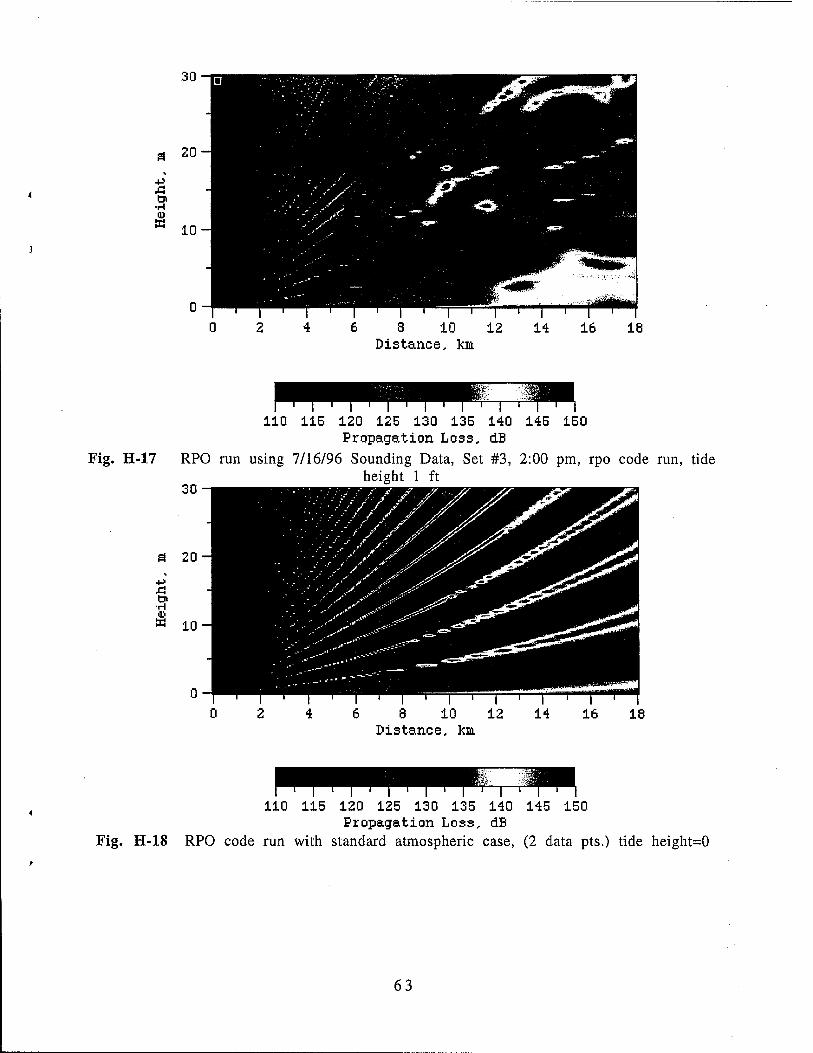
Fig. H-17
i—l—r
110 115 120 125 130 135 140 145 150 Propagation Loss, dB
RPO run using 7/16/96 Sounding Data, Set #3, 2:00 pm, rpo code run, tide height 1 ft
6 8 10 12 Distance, km.
14 16 18
1 I ' 110 115 120 125 130 135 140 145 150
Propagation Loss, dB Fig. H-18 RPO code run with standard atmospheric case, (2 data pts.) tide height=0
63

Average Signal Level (-dB) I
Tide Height, ft |
0Ü
4> > <l>
CO c
CO
> <
60
55
50
45
40
35
30
-I—i 1 r SSLS2
set* 1j 10:20 km
12:20|fm ' set« ' ! 2:00 pm I
T—i—i—r
i .TT..*s«w.^w-rr •
_l I I L_ X i ■ ■ i i I i_
2.5
2
1.5 £ I
1 <£ a1
0.5
0
■0.5 16.4 16.5 16.6 16.7
Time, days
16.8 16.9
Fig. H-19 Tilghman Island Radar Signal Level and Tide Height, 7/16/96
60 -i 1 1 1 r -i 1-
Tide Height, ft |
average Signal Level (-dB)
2.5
2
Time, days Fig. H-20 Tilghman Island Radar Signal Level and Tide Height, 7/16/96
64

APPENDIX I. Weather Data Sources
Various sources are available over the internet for obtaining weather data. This data is usually presented on a real time basis, so archiving is necessary to use old data. Tide data, radiosonde data, weather station data, satellite visible and infrared (IR) pictures (GOES satellite), and wave height and water vapor data (TOPEX satellite) are available.
Temperature, wind speed, wind direction, humidity, water temperature, dew point, and barometric pressure are weather data taken daily at CBD. Weather information about the Bay can also be accessed over the telephone from the weather bureau. By calling 703-260-0505, a forecast is given for the Chesapeake Bay area that includes temperature, wind speed and direction, and wave height.
Moon phase information is located in the local paper (Washington Times or Washington Post). They also give high tide times.
Tide data can be accessed by telneting to WLNET2.NOS.NOAA.GOV. The word GUEST is used as a username. Archived six-minute water level data can then be accessed from various stations. Local stations are at Annapolis and Solomon's Island. Tide data for CBD can then be approximated by subtracting one hour from the Annapolis data. (Tide map shows 1 hour difference).
The Northeast Regional Climate Center maintains archived weather data for numerous sites including the Baltimore-Washington International airport (BWI) and the Patuxant Naval Air Station. Archived data is obtained with a small fee. Daily data is also available and can be archived independently. The internet address is
http://met-www.cit.cornell.edu/nrcc_home.html.
Topex satellite data including wave height and water vapor content can be accessed with the internet address:
http://podaac-www.jpl.nasa.gov/topex/
Michigan State University has current weather maps and movies available for downloading. They make composite weather maps from GOES satellite data. Updates are every 3 and 6 hours. Of interest to this project is the Worldwide Montage and Worldwide IR Composite pictures. The internet address is: http://rs560.cl.msu.edu/weather/
Another good site for weather information is the WeatherNet WeatherSites page on the internet. It gives a list of lots of weather sites.
http://cirrus.sprl.umich.edu/wxnet/servers.html
Radiosonde data is presented at various sites. Use search engine under 'radiosonde'.
65

Weather archiving has been ongoing since January 1996. This data can be used in the analysis of open-ocean tracks. The archiving of data off the internet was automated. It includes whole world satellite visible and IR imagery as well as Doppler radar information where available. Hourly weather station data is also archived for various sites in the DELMARVA area. Figure 1-1 shows GOES 8 data. Figure 1-2 shows a composite of satellite and Doppler radar images.
Moderate storm: overcast and moderate rainfall
Large storm: at center of storm, heavy rainfall and downpours likely
Fig. 1-1 GOES-8 Image
Fig. 1-2 NEXRAD Doppler radar imagery (color areas showing precipitation)
66