Sea Level Rise, Hydrodynamic Modeling, and Inundation
110
Humboldt Bay: Sea Level Rise, Hydrodynamic Modeling, and Inundation Vulnerability Mapping Prepared for State Coastal Conservancy, and Coastal Ecosystems Institute of Northern California Final Report April 2015 Prepared by Northern Hydrology & Engineering
Transcript of Sea Level Rise, Hydrodynamic Modeling, and Inundation

Humboldt Bay: Sea Level Rise, Hydrodynamic Modeling, and Inundation Vulnerability Mapping
Prepared for
State Coastal Conservancy, and
Coastal Ecosystems Institute of Northern California
Final Report
April 2015
Prepared by
Northern Hydrology & Engineering
Humboldt Bay: Sea Level Rise, Hydrodynamic Modeling, and Inundation Vulnerability Mapping
Final Report
April 2015
Prepared for
State Coastal Conservancy
1330 Broadway, 13th Floor
Oakland, CA 94612-2530
and
Coastal Ecosystems Institute of Northern California
PO Box 806
Bayside, CA 95524
Prepared by and under the supervision of Jeffrey K. Anderson, PE (C50713)
Northern Hydrology & Engineering
P.O. Box 2515 McKinleyville, CA 95519
Cover figure: Humboldt Bay predicted water level for year 2012 (left figure), and resulting 100-yr vulnerability inundation map (right figure).

i
Table of Contents
1 Introduction .................................................................................................. 1
Background ............................................................................................................................................... 1
Purpose and Scope ................................................................................................................................... 3
Humboldt Bay Physical Description .......................................................................................................... 3
Previous Humboldt Bay Sea Level Rise Mapping ..................................................................................... 5
General SLR Hydrodynamic Modeling and Inundation Mapping Approach ............................................ 6
Disclaimer ................................................................................................................................................. 6
Acknowledgments .................................................................................................................................... 6
2 Sea Level Change in the Humboldt Bay Region .............................................. 8
General Concepts and Definitions ............................................................................................................ 8
Global Climate System Change ............................................................................................................... 10
Past and Present Global Sea Level Rise .................................................................................................. 13
Past and Present Regional Sea Level Rise ............................................................................................... 17
Past and Present Relative Sea Level Rise ................................................................................................ 22
Projections of Sea Level Rise .................................................................................................................. 33
3 Hydrodynamic Model Methods and Configuration ...................................... 43
Model Formulation ................................................................................................................................. 43
Model Grid .............................................................................................................................................. 47
Model parameters and Initial conditions ............................................................................................... 48
4 Hydrodynamic Model Ocean Boundary Condition ....................................... 50
Tidal Observations .................................................................................................................................. 50
100-year Long Detrended Hourly Sea Level Height Series ..................................................................... 51
Adequacy of 100-yr Hourly Sea Level Height Series ............................................................................... 53
Sea Level Rise Modeling Scenarios ......................................................................................................... 60
5 Hydrodynamic Model Results ..................................................................... 62
Available Hourly Tidal Observations in Humboldt Bay ........................................................................... 62
Water Level Comparisons ....................................................................................................................... 63
Summary ................................................................................................................................................. 69
6 Sea Level Rise Inundation Vulnerability Mapping ........................................ 74
Post-Processing 2D Hydrodynamic Model Results ................................................................................. 74
Inundation Vulnerability Mapping ......................................................................................................... 76
Humboldt Bay Year 2012 Mean High Water Map .................................................................................. 80
Inundation Vulnerability Mapping Distribution Files ............................................................................. 82
7 Discussion ................................................................................................... 83
Inundation Vulnerability Map Limitations .............................................................................................. 83

ii
Humboldt Bay Predicted Water Levels for Existing and Future Sea Levels ............................................ 84
Areas Vulnerable to Inundation for Existing and Future Sea Levels ...................................................... 89
Interpretation of Inundation Vulnerability Maps ................................................................................... 93
8 Conclusions, Summary and Recommendation ............................................. 95
Conclusions and Summary ..................................................................................................................... 95
Recommendations .................................................................................................................................. 96
9 References .................................................................................................. 98
10 Glossary .................................................................................................... 105

1
1 Introduction
Background
Sea level rise is one of the most evident and problematic consequences of global climate change.
As the earth’s climate warms, sea levels increase primarily from thermal expansion of a warmer
ocean and melting land ice (NRC, 2012). In California, sea level rise (SLR) will threaten and
directly affect vulnerable coastal ecosystems, bays and estuaries, coastal communities and
infrastructure due to increased flooding, gradual inundation, and erosion of the coastal
shorelines, cliffs, bluffs and dunes (Russell and Griggs, 2012). If sea level continues to rise at
present rates, impacts identified in this report could take decades or longer to occur. However, a
troublesome aspect of climate change and the rapid warming of the earth’s atmosphere and ocean
is the potential for SLR to accelerate to high rates over a short period of time, in which case the
identified impacts could happen within a much shorter period (years to decades).
In 2008, California Governor Schwarzenegger issued Executive Order S-13-08 directing state
agencies to plan for SLR and corresponding impacts. Following the executive order, planning
for the inevitable effects of SLR to California’s communities and regions has become a priority
for many local coastal governments and state agencies.
Humboldt Bay is located in northernmost California approximately 160 km south of the Oregon
border and 420 km north of San Francisco (Figure 1-1). The bay contains numerous aquatic and
terrestrial ecosystems that support a diversity of wildlife species, Native American cultures, a
number of small towns and communities (e.g. Eureka and Arcata), and an economy dependent
on natural resources (Schlosser et al., 2009). Beginning in 2006, with funding from the State
Coastal Conservancy (SCC), a group of local scientists, resource managers, and stakeholders
established a Science Advisory Team to explore how ecosystem-based management could be
applied to Humboldt Bay. In 2008, with funding from the David and Lucile Packard Foundation,
the Advisory Team undertook a formal strategic planning effort in Humboldt Bay. A
culmination of these efforts was the Humboldt Bay Strategic Plan and the formation of the
Humboldt Bay Initiative (Schlosser et al., 2009). The strategic plan identified climate change
and associated SLR as a very high threat to Humboldt Bay, and further noted that these threats
were not well understood nor had they been assessed.
Recently, the SCC began funding a coordinated planning effort to identify SLR vulnerabilities
and develop adaptation strategies for Humboldt Bay, known as the Humboldt Bay Sea Level
Rise Adaptation Planning (HBSLRAP) project. The first phase of this work was a Humboldt
Bay shoreline inventory, mapping and vulnerability assessment conducted by Trinity Associates
(Laird, 2013) that identified portions of the bay’s shorelines vulnerable to failure and
overtopping from current sea levels. The second phase, which was sponsored by the Coastal
Ecosystems Institute of Northern California (CEINC), consisted of two components: identifying
additional SLR vulnerabilities in Humboldt Bay through a detailed technical study, and SLR

2
adaptation planning and risk assessment, co-sponsored by the Humboldt County Public Works
(County) and Humboldt Bay Harbor, Recreation and Conservation District (District).
Figure 1-1 Humboldt Bay location map.
The County and District convened an Adaptation Planning Working Group (APWG) for the
adaptation planning component of the project, with Trinity Associates serving as the adaptation
planning consultant for the working group. The APWG consists of members from the District,
County, Cities of Arcata and Eureka, California Coastal Commission, State Coastal
Conservancy, Wiyot Tribe, Humboldt Bay National Wildlife Refuge, California Department of
Fish and Wildlife, U.S. Fish and Wildlife Service, Bureau of Land Management, California
Department of Transportation, California Sea Grant Extension, Humboldt County Farm Bureau,
Humboldt County Resources Conservation District, National Resources Conservation Service,
North Coast Regional Land Trust, CEINC, Trinity Associates, U.C. Agricultural Extension, and
Northern Hydrology & Engineering. The goal of the APWG is to support informed decision-
making and encourage a unified, consistent regional adaptation strategy to address impacts to
critical assets associated with SLR in the Humboldt Bay region.

3
The project component to identify additional SLR vulnerabilities in Humboldt Bay was led by
Northern Hydrology and Engineering (NHE) and consisted of the following work products:
1. SLR hydrodynamic modeling to develop inundation vulnerability maps of areas
surrounding Humboldt Bay vulnerable to inundation from existing and future sea levels
(described in this report).
2. A seamless topographic/bathymetric digital elevation model (DEM) of Humboldt Bay
using the recent 2009-2011 California Coastal Conservancy LiDAR Project Hydro-
flattened Bare Earth DEM (California Coastal DEM) and various subtidal bathymetric
data sets to support the modeling efforts. Pacific Watershed Associates (PWA)
conducted this work in 2014.
3. A conceptual groundwater model to analyze the effects of SLR on groundwater levels
and saltwater intrusion in the Eureka-Arcata coastal plain. Dr. Robert Willis conducted
this work in 2014.
Purpose and Scope
Sea level rise already threatens many areas surrounding Humboldt Bay that are currently
protected by the natural shoreline, levees, and road or railroad grades from flooding by extreme
high tides and storm events, and many more vulnerable areas will be threatened by SLR within
the century. If SLR rates accelerate as projected, these vulnerable areas could see routine
flooding within the next few decades, particularly if levees or other shoreline barriers fail. The
purpose of this project is to (1) conduct detailed hydrodynamic modeling in Humboldt Bay to
determine average high water levels and extreme high water level event probabilities for existing
sea levels and SLR scenarios, and (2) develop inundation maps of areas surrounding the bay that
are vulnerable to inundation from existing and future sea levels. The ultimate goal of this project
is to provide the APWG and general public information on how SLR may affect high water
levels in Humboldt Bay, including inundation vulnerability maps in a user-friendly format.
For the remainder of this study, the Humboldt Bay shoreline refers to the natural shoreline, and
the portions of shoreline consisting of levees, road and railroad grades, and other man-made
barriers or structures.
Humboldt Bay Physical Description
Humboldt Bay can best be described as a tidally driven, multi-basin, bar-built, coastal lagoon
(Figure 1-2), and is the second largest enclosed bay in California (Costa, 1982; Costa and
Glatzel, 2002; Schlosser and Eicher, 2012). The bay is separated from the Pacific Ocean by two
long, narrow sand spits (North Spit and South Spit), and is connected to the ocean by the
stabilized, twin-jettied Entrance Channel. The first attempts to stabilize the entrance began in
1889, and dredging of interior harbor channels began as early as 1881 (Costa and Glatzel, 2002).

4
Figure 1-2 Humboldt Bay physical setting and mean high water edge (blue line).
Humboldt Bay contains three distinct bays (Figure 1-2), Entrance Bay, North (or Arcata) Bay,
and South Bay (Costa 1982; Costa and Glatzel, 2002). Entrance Bay is connected to the ocean
through the Entrance Channel, which is maintenance dredged by the U.S. Army Corps of
Engineers. South Bay is directly connected to Entrance Bay through a natural constriction and
the dredged Fields Landing Channel. North Bay is connected to Entrance Bay via the long,
narrow dredged North Bay Channel. The North Bay Channel splits into the dredged Samoa and
Eureka Channels, just before connecting with North Bay.
Humboldt Bay is relatively shallow, with 70% of the bay comprised of tidal mud flats that are
exposed during low tide (Costa, 1982). The mud flats are predominately in North and South
Bays, and only Entrance Bay and the lower portions of North Bay Channel maintain an
North (Arcata) Bay
South Bay
Entrance Bay
North Bay Channel
Samoa Channel
Eureka Channel
Mad River Slough
Eureka
Arcata
Entrance Channel
Fields Landing Channel

5
approximate constant surface area over a tide cycle. The water surface area of Humboldt Bay is
approximately 64.8 km2 at high tide and 20.7 km
2 during low tide (Costa, 1982).
The drainage basin of Humboldt Bay is approximately 578 km2, a relatively small basin for a bay
of its size. Although a number of small streams flow into the bay, the annual freshwater input to
the bay is small, on the order of the tidal prism (Costa, 1982). The tidal prism is approximately
9.63 to 9.91 x 10⁷ m
3 during a spring tide range and about 70% less over a mean tide range
(Costa and Glatzel, 2002). North Bay contributes approximately 50% of the tidal prism, and
about 30% for South Bay.
Humboldt Bay tides are mixed semidiurnal, and show tidal amplification and phase lag with
distance from the entrance (Costa, 1982; Costa and Glatzel, 2002). Due to the small freshwater
inflow, the general circulation of Humboldt Bay is dominated by tidally driven flows modified
by the bathymetry (Costa, 1982), with estuarine conditions typically only found within the small
stream mouths and slough channels (Costa and Glatzel, 2002). The general circulation patterns
can be affected on daily and seasonal time scales by waves entering through Entrance Channel
(primarily influencing Entrance Bay), internally generated wind waves, and density differences
(Costa, 1982). Humboldt Bay is typically well mixed vertically, and normally consists of
unstratified marine water (Costa and Glatzel, 2002).
Previous Humboldt Bay Sea Level Rise Mapping
A previous study conducted by the Pacific Institute (Herberger et al., 2009) mapped flood and
coastal erosion hazard zones along the California coast for year 2000 existing conditions and
year 2100 with 1.4 m (55 inches) of SLR based on the Cayan et al. (2009) SLR estimate for the
Intergovernmental Panel on Climate Change (IPCC) A2 emission scenario. Phillip Williams and
Associates Ltd. (2009), now ESA PWA, provided the coastal erosion hazards assessment, and
compiled a statewide Base Flood Elevations (BFE) layer to support the flood hazard analysis
conducted by Pacific Institute. As defined by FEMA, the BFE is the 1% (100-yr) annual chance
flood elevation, and for coastal areas is the 1% total water level (TWL) which consists of the still
water elevation (SWL) and wave effects. The BFE layer consisted of published FEMA BFEs for
California, with data gaps filled using professional judgment and/or local knowledge and
experience. The Pacific Institute flood hazard maps developed for Humboldt Bay used a single
water elevation value (bathtub approach) to map flood zones in the bay. Review of the BFE
layer (available at http://www2.pacinst.org) indicates that the mapped year 2000 BFE value was
2.90 m (9.5 ft) referenced to the North American Vertical Datum of 1988 (NAVD88), and the
year 2100 BFE value would have been 4.3 m (2.9 m + 1.4 m SLR). Since the California Coastal
DEM was not available until 2012, it was assumed that the flood hazard maps produced by
Pacific Institute in 2009 for Humboldt Bay relied on the USGS National Elevation Dataset 10-m
resolution topography, which has a stated vertical accuracy of ±7.5 m (Herberger et al., 2009).

6
General SLR Hydrodynamic Modeling and Inundation Mapping Approach
The Humboldt Bay SLR modeling and inundation mapping conducted in this study was built
from the general approach used by Knowles (2010) for similar work done in San Francisco Bay.
A hydrodynamic model was used to predict water levels within the existing shoreline of
Humboldt Bay for five SLR scenarios: year 2012 existing sea levels and half-meter SLR
increments of 0.5, 1.0, 1.5 and 2.0 m. The hydrodynamic model was forced by a 100-yr long
stationary hourly sea level height series developed for Crescent City tide gauge. The 100-yr
hourly series accounts for astronomical tides, and varying effects including wind, sea level
pressure, and El Niño variability. The 100-yr series was incremental adjusted for each half-
meter SLR scenario. Each hydrodynamic model simulation produced 100 years of predicted
water levels throughout the bay. Estimates of average high water levels and annual exceedance
probabilities of extreme high water levels were determined bay-wide for each of the five SLR
scenarios.
Using the model results, inundation vulnerability maps of areas surrounding Humboldt Bay
vulnerable to inundation from existing and future sea levels were produced for the estimated
average water levels and extreme high water level events from the five SLR scenarios. The
inundation maps identified areas surrounding Humboldt Bay currently protected from inundation
by the shoreline, levees or other barriers, but are vulnerable and at risk to flooding from future
sea levels. The inundation vulnerability mapping relied on the recent high resolution California
Coastal DEM (PWA, 2014).
Disclaimer
The sea level rise modeling, analysis, and inundation vulnerability mapping conducted in this
study are intended for use as planning-level tools to illustrate the areas surrounding Humboldt
Bay vulnerable to existing and future sea levels. The inundation vulnerability maps identify
potential future inundation conditions that could occur if nothing is done to adapt to, or prepare
for sea level rise.
The 100-year extreme high water surface elevations presented in this report do not represent
what FEMA defines as the 1% annual base flood elevation, which includes wave effects. The
extreme high water level events presented in this report correspond approximately to what
FEMA defines as still water elevations.
Acknowledgments
This study was funded by the State Coastal Conservancy, and sponsored by the Coastal
Ecosystems Institute of Northern California. The principal author, Jeff Anderson, would like to
acknowledge the following individuals. First, a special thanks to Susan Schlosser who’s
diligence and drive for all things Humboldt Bay paved the way for this study. Thanks to Corin
Pilkington of NHE for development of the inundation vulnerability maps. Thanks to the

7
following individuals who reviewed and commented on this report in draft form: Jill Demers,
CEINC; Joel Gerwein, SCC; Dr. Sharon Kramer, CEINC; Darren Mierau, CEINC; Rose
Patenaude, NHE; Becky Price-Hall, CEINC; Hank Seemann, Humboldt County; Susan
Schlosser, CEINC; and Dr. Frank Shaughnessy, CEINC. Thanks to Robert Willis for providing
initial feedback on the modeling approach for this study, and Whelan Gilkerson of PWA for
development of the Humboldt Bay digital elevation model (DEM). Finally, thanks to Aldaron
Laird of Trinity Associates for always asking questions.

8
2 Sea Level Change in the Humboldt Bay Region
The Humboldt Bay region, which for this report includes the coasts of Humboldt and Del Norte
Counties, is experiencing the combined effects of global sea level rise, regional sea level height
variability from seasonal to multidecadal ocean-atmosphere circulation dynamics (e.g. El Niño
Southern Oscillation), and relatively large tectonic vertical land motions associated with the
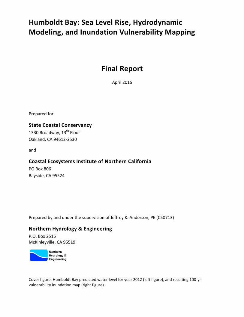
Cascadia subduction zone (CSZ) (Figure 2-1). These large tectonic motions along the southern
CSZ create the highly variable and opposing sea level trends observed between Humboldt Bay
and Crescent City. Recent estimates of land subsidence by Patton et al. (2014) indicate that
Humboldt Bay has the highest local sea level rise rate in California, approximately two to three
times higher than the long-term global rate. In contrast, the land in Crescent City (109 km north)
is uplifting faster than long-term global sea level rise, which causes a negative or decreasing
local sea level rise rate.
The purpose of this chapter is to provide an overview of global and regional sea level change,
with an emphasis on the physical processes locally effecting sea levels in the Humboldt Bay
region. This overview relies on the climate and sea level change literature, specifically the 2013
Intergovernmental Panel on Climate Change (IPCC) Fifth Assessment Report, the 2012 National
Resource Council (NRC) Sea Level Rise for the Coasts of California, Oregon, and Washington
report, and the scientific and technical literature specific to the U.S. Pacific Northwest (PNW)
coast (Northern California (north of Cape Mendocino), Oregon and Washington), and the
Humboldt Bay region.
General Concepts and Definitions
Mean Sea Level
Mean sea level (MSL) is the average ocean level at a specific location over a known period of
time. When MSL is estimated at a tide gauge from the hourly sea level height record over the
19-year National Tidal Datum Epoch (NTDE) period, it is known as the MSL tidal datum. The
current tidal epoch is the 1983-2001 NTDE. MSL can change (rise or fall) over temporal and
global, regional and local spatial scales.
Global Mean Sea Level
Global (or eustatic) mean sea level (GMSL) is the average height of the earth’s oceans, and
GMSL changes globally due to (1) changes in the shape of the ocean basins, (2) a change in
ocean volume due to changes in the total mass of water in the ocean (barystatic), and (3) a
change in ocean volume from changes in ocean water density (steric) (IPCC, 2013a).
Thermosteric refers to density changes from ocean temperature changes, while halosteric defines
density changes from changes in ocean salinity.
9
Figure 2-1 Tectonic plate boundaries along the U.S. west coast, and the location of Humboldt Bay and
Crescent City relative to the Cascadia subduction zone. Tectonic boundary data
downloaded from http://earthquake.usgs.gov/learn/kml.php.
Long-term reconstructions of GMSL change (e.g. Church and White, 2011) generally rely on the
longest tide gauge records located on relatively stable land (Zervas, 2013), which are then
adjusted for ocean basin changes, such as the land motion associated with the global glacial
isostatic adjustment.
Regional Mean Sea Level
Regionally, sea level change may differ from GMSL due to meteorological effects (for example
storms) and natural climate variability, such as the El Niño Southern Oscillation, which alters
surface winds, ocean heating, and ocean currents (NRC, 2012; Church et al., 2013). Regional
mean sea level (ReMSL) is the average sea level over a region of the earth’s oceans, such as the

10
U.S. west coast. In this report, ReMSL does not include the effects of vertical land motion, such
as plate tectonic motion.
Relative Sea Level
Relative sea level (RSL), or local sea level, is the sea level measured by a tide gauge relative to a
specific point on land. Tide gauges measure the combined effects of ocean volume change
(GMSL), ocean and climate variability (ReMSL), and vertical land motion. The change in RSL
is what coastal areas experience, and is the quantity used for assessing and planning for the
coastal impacts from sea level change (NRC, 2012; Church et al., 2013).
Vertical Land Motion
Global, regional and local vertical land motions (VLM) effect RSL change, and are responsible
for most of the regional RSL trend differences observed between tide gauges (Zervas, 2009).
Examples of VLM include glacial isostatic adjustment, plate tectonic land-level changes (seismic
and interseismic), and land subsidence (e.g. soil compaction and groundwater extraction).
Glacial isostatic adjustment (GIA) is the deformation of the earth in response to melting of the
large continental ice sheets that covered much of North America and Europe (Peltier, 1990),
during the last glacial maximum that occurred about 20,000 years ago (Kominz, 2001).
Estimates of GMSL rise trends are generally adjusted for vertical GIA using GIA models. For
example, Peltier (2002, 2009) estimates the global average GIA at -0.3 mm/yr (a downward
VLM).
Regional and local VLM, such as tectonic land-level changes, can be much larger than those
associated with GIA models (Zervas, 2013). Researchers have documented interseismic tectonic
uplift rates from plate locking along the CSZ that are an order-of-magnitude greater than the
global GIA rate (Mitchell et al., 1994; Burgette et al., 2009). Along the PNW coast, the tectonic
land-level changes associated with the CSZ strongly affect RSL changes, indicating both
submergent and emergent stretches of coast (Komar et al., 2011).
Global Climate System Change
In 2013, the IPCC completed its Fifth Assessment Report (AR5). The AR5 builds upon the 2007
IPCC Fourth Assessment Report (AR4), and considers the climate science and research findings
since AR4. Conclusions from the AR5 climate change science shows (95% confidence) that
human activity is the dominant cause of the observed global climate system warming since the
mid-20th century. Climate change will undoubtedly affect global climate such as temperature
and precipitation patterns, ocean temperatures and chemistry, ocean-climate variability, and sea
level rise. The following excerpts are key climate system change summary statements from the
IPCC AR5 Summary for Policymakers report (IPCC, 2013b).

11
“Each of the last three decades has been successively warmer at the
Earth’s surface than any preceding decade since 1850 (Figure 2-2). In the
northern hemisphere, 1983-2012 was likely the warmest 30-year period of
the last 1400 years (medium confidence).”
“Ocean warming dominates the increase in energy stored in the climate
system, accounting for more than 90% of the energy accumulated between
1971 and 2010 (high confidence). It is virtually certain that the upper
ocean (0−700 m) warmed from 1971 to 2010, and it likely warmed
between the 1870s and 1971.”
“Over the last two decades, the Greenland and Antarctic ice sheets have
been losing mass, glaciers have continued to shrink almost worldwide, and
Arctic sea ice and Northern Hemisphere spring snow cover have continued
to decrease in extent (high confidence).”
“The rate of sea level rise since the mid-19th century has been larger than
the mean rate during the previous two millennia (high confidence). Over
the period 1901 to 2010, global mean sea level rose by 0.19 [0.17 to 0.21]
m.”
“The atmospheric concentrations of carbon dioxide, methane, and nitrous
oxide have increased to levels unprecedented in at least the last 800,000
years. Carbon dioxide concentrations have increased by 40% since pre-
industrial times, primarily from fossil fuel emissions and secondarily from
net land use change emissions. The ocean has absorbed about 30% of the
emitted anthropogenic carbon dioxide, causing ocean acidification (Figure
2-3).”
“Total radiative forcing is positive, and has led to an uptake of energy by
the climate system. The largest contribution to total radiative forcing is
caused by the increase in the atmospheric concentration of CO2 since
1750.”
“Continued emissions of greenhouse gases will cause further warming and
changes in all components of the climate system. Limiting climate change
will require substantial and sustained reductions of greenhouse gas
emissions.”

12
Figure 2-2 (a) Observed 1850 to 2012 global mean combined land and ocean surface temperature
anomalies (relative to the mean of 1961-1990) from three datasets. Top panel is the annual
mean values, and bottom panel are the decadal mean values with uncertainty for one
dataset (black). (b) Map of observed surface temperature change (1901 to 2012) derived
from temperature trends (orange line in panel a). (Figure from IPCC (2013b), Figure SPM.1)

13
Figure 2-3 (a) Observed atmospheric carbon dioxide (CO2) concentrations for Mauna Loa (red line) and
South Pole (black line) since 1958. (b) Ocean surface observed partial pressure of dissolved
CO2 (blue lines), and in situ pH (green lines) which is an indicator of ocean acidification.
Measurements from Atlantic Ocean (dark blue and dark green, and blue and green) and
Pacific Ocean (light blue and light green). (Figure from IPCC (2013b), Figure SPM.4)
Past and Present Global Sea Level Rise
Global sea levels have been increasing for 20,000 years since the last ice age (Russell and
Griggs, 2012; Kominz, 2001), although at relatively low rates (~ 0.1 mm/yr) over the last two
millennia (NRC, 2012). There is high confidence, based on proxy records (e.g. salt marsh
sediments) and instrumental sea level data, that GMSL rise increased in the late 19th to early
20th century from relatively low rates over the previous two millennia to higher rates today
(Church et al., 2013). As noted earlier, sea levels are increasing globally due to thermal

14
expansion from ocean warming and increases in ocean mass from melting land ice caused by
warming of the earth’s climate.
Reconstructions of late 19th, 20th and early 21st century GMSL rise have been made by
numerous investigators (e.g. Jevrejeva et al., 2008; Church and White, 2011; Ray and Douglas,
2011) using tide gauge records, starting in the late 1800s, and the more recent satellite-based
radar altimeter measurements since the early 1990s. Only results of the reconstructed GMSL
time series (1880 to 2010) and satellite altimeter data (1992 to 2010) of Church and White
(2011) are presented in this study (Figure 2-4 and Table 2-1). As noted by Rhein et al. (2013),
other long-term GMSL reconstructions (e.g. Jevrejeva et al., 2008; Ray and Douglas, 2011; and
others) provide similar long-term rates of GMSL rise as compared to the Church and White
(2011) estimate. To account for ocean volume variability, the Church and White (2011) GMSL
estimates removed the GIA signal and adjusted sea levels for atmospheric pressure variations
(inverse barometer effect).
Figure 2-4 Yearly average reconstructed global mean sea level (GMSL) for 1880 to 2010 with one
standard deviation uncertainty bounds, and satellite altimeter data for 1993 to 2010
(Church and White, 2011). The reconstruction is set to zero in 1990, and satellite altimeter
data match the reconstructed time series over 1993. Data downloaded from
http://www.cmar.csiro.au.
-25
-20
-15
-10
-5
0
5
10
1880 1890 1900 1910 1920 1930 1940 1950 1960 1970 1980 1990 2000 2010
Wat
er
Leve
l (cm
)
Year
Yearly average reconstructed GMSL GMSL one standard deviation uncertainty
Satellite altimeter

15
Table 2-1 Estimated global mean sea level (GMSL) rise trends and uncertainty range for different time
periods. Data from Church and White (2011), and Table 3.1 of Rhein et al. (2013).
Time Period GMSL Rise Trend (mm/yr) Source
1901 to 1990 1.5 [1.3 to 1.6] Tide gauge reconstruction
1901 to 2010 1.7 [1.5 to 1.9] Tide gauge reconstruction
1936 to 2010 1.8 [1.5 to 2.1] Tide gauge reconstruction
1961 to 2010 1.9 [1.5 to 2.3] Tide gauge reconstruction
1971 to 2010 2.0 [1.5 to 1.9] Tide gauge reconstruction
1993 to 2010 2.8 [2.3 to 3.3] Tide gauge reconstruction
1993 to 2010 3.2 [2.8 to 3.6] Satellite altimetry data
The 2013 IPCC AR5 states it is very likely (90 to 100% probability) that the rate of GMSL rise
between 1901 and 2010 was 1.7 ± 0.2 mm/yr, and increased to 3.2 ± 0.4 mm/yr between 1993
and 2010 (Rhein et al., 2013). During the 20th century, there is high confidence that the
dominant contributors to GMSL rise were ocean thermal expansion and glacier mass loss
(Church et al., 2013).
The IPCC AR5 scientific work further documented the observed contributions to GMSL rise for
the 1993 to 2010 period from ocean thermal expansion, melting land ice, and land water storage
(Table 2-2), with thermal expansion and land ice melting being the dominant contributors (Rhein
et al., 2013; Church et al., 2013).
To better understand GMSL change and contributions a number of global observation systems
have been deployed over the last two decades, which include (1) satellite radar altimetry to
measure sea level height, (2) the Argo Project global ocean array of free-drifting profiling floats
that measure temperature and salinity in the upper 2,000 m of the ocean, and (3) the Gravity
Recovery and Climate Experiment (GRACE) satellites that measure the Earth's gravity field and
can detect mass changes in the oceans and ice sheets. Between 1993 and 2010, the total
observed contributions to GMSL rise was estimated at 2.8 ± ~0.5 mm/yr, which is consistent
with the tide gage reconstructions (2.8 ± 0.5 mm/yr) and the satellite altimetry data (3.2 ± 0.4
mm/yr) for the same period (Table 2-2).

16
Table 2-2 Observed global mean sea level (GMSL) rise trends, observed contributions to GMSL rise
and model-based contributions to GMSL rise for the 1993 to 2010 period based on the
2013 IPCC AR5. Uncertainties are 5 to 95%. GMSL rise trends from Church and White
(2011); observed contributions from Table 3.1 of Rhein et al. (2013); observed and model-
based contributions from Table 13.1 of Church et al. (2013).
Source Trend/Contribution for 1993 to 2010 (mm/yr)
Observed GMSL rise
Tide gauge reconstruction 2.8 [2.3 to 3.3]
Satellite altimeter data 3.2 [2.8 to 3.6]
Observed GMSL Contributions
Ocean thermal expansion 1.1 [0.8 to 1.4]
Glaciers (except in Greenland and Antarctica) 0.76 [0.39 to 1.13]
Greenland ice sheet and glaciers 0.33 [0.25 to 0.41]
Antarctic ice sheet 0.27 [0.16 to 0.38]
Land water storage 0.38 [0.26 to 0.49]
Total of contributions 2.8 [2.3 to 3.4]
Modeled GMSL Contributions
Ocean thermal expansion 1.49 [0.97 to 2.02]
Glaciers (except in Greenland and Antarctica) 0.78 [0.43 to 1.13]
Glaciers in Greenland 0.14 [0.06 to 0.23]
Total of contributions including land water storage 2.8 [2.1 to 3.5]
As noted by Church et al. (2013), the ability to reproduce observed GMSL change since 1993
from the observed ocean budget (ocean mass and thermosteric changes) demonstrates a
significant advancement since the 2007 IPCC AR4 (Meehl et al., 2007) in understanding the
contributions to GMSL change (Figure 2-5).

17
Figure 2-5 Observed global mean sea level (GMSL) from satellite altimetry (blue line), observed ocean
mass changes from GRACE satellites (green line), and observed thermosteric sea level
change from Argo floats (red line) for 2005 to 2012. The dashed black line is the summed
contributions of GRACE and Argo observations. (Figure from Church et al. (2013), Figure
13.6)
Past and Present Regional Sea Level Rise
Spatial patterns in sea level change can differ from GMSL values due to regional ocean and
climate processes, such as El Niño Southern Oscillation, which effects ocean circulation patterns
on seasonal to multi-decadal timescales and redistributes ocean mass and temperature (Cayan et
al., 2008; Bromirski et al., 2011; NRC, 2012; Church et al., 2013; Rhein et al., 2013). For
example, Figure 2-6 shows the monthly MSL trends, as reported by National Oceanic
Atmospheric Administration (NOAA) Center for Operational Oceanographic Products and
Services (CO-OPS) for three long-term tide gauge sites (Seattle, San Francisco and San Diego)
along the U.S. west coast that are located on relatively tectonically stable ground (Cayan et al.,
2008; Burgette et al., 2009; Bromirski et al., 2011). Each tide gauge record is over 100-yrs long,
beginning in 1898 for Seattle, 1897 for San Francisco, and 1906 for San Diego, which coincides

18
well with the 1901 to 2010 GMSL reconstruction period of Church et al. (2011). The RSL rise
trends for these three U.S. west coast tide gauge locations are very consistent, ranging from 1.89
to 2.04 mm/yr (average ~2.0 mm/yr), which is greater (18% increase) than the 1901 to 2010
GMSL trend of 1.7 mm/yr (Table 2-1). This implies that over the instrument period, ReMSL
rise along the U.S. west coast has been greater than GMSL rise for the same general period.
Processes Affecting Regional Sea Level Rise on the U.S. West Coast
The NRC (2012) report addressed sea level variability along the coasts of California, Oregon and
Washington. Monthly mean sea levels vary along the MSL trend line (Figure 2-6) due to natural
climate and ocean variability. The following subsections briefly summarize the dominant
processes affecting ReMSL change in the Pacific Ocean along the U.S. west coast, taken from
the NRC (2012) report and other scientific literature.
Seasonal to Interannual Variability
The El Niño Southern Oscillation (ENSO) is the most important coupled ocean-atmosphere
phenomenon that causes seasonal to interannual timescale global climate variability (Wolter and
Timlin, 2011). ENSO is the dominant cause of sea level variability along the U.S. west coast
(Komar et al., 2011; Bromirski et al., 2011; NRC, 2012), with higher sea levels during the
warmer El Niño phase, and lower levels during the cooler La Niña phase (Figure 2-7). Strong El
Niño events effect wind and ocean circulation, reducing upwelling and producing warmer than
normal ocean temperatures along the U.S. west coast, which can raise mean winter water levels
by 0.2 to 0.3 m for several months (Komar et al, 2011). This winter seasonal increase is larger
than the 20th century GMSL rise of 0.17 m (Table 2-1). El Niño events are generally associated
with a more active winter storm period along the U.S. west coast (NRC, 2012).
Seasonal coastal current and wind patterns (e.g. upwelling) also produce seasonal variations in
sea level heights (known as the average seasonal cycle) due to ocean temperature and density
changes (Komar et al., 2011). Both ENSO and the average seasonal cycle will be discussed in
more detail for the Humboldt Bay region in following sections of this chapter.

19
Figure 2-6 Observed monthly relative sea level (RSL) rise trends from NOAA tide gauge records for Seattle, San Francisco and San Diego. These
tide gauge sites are located on relatively tectonically stable ground. Data and figures downloaded from NOAA CO-OPS at
http://tidesandcurrents.noaa.gov.

20
Figure 2-7 (A) Multivariate ENSO index (MEI), and (B) Pacific Decadal Oscillation (PDO) index from
1900 to March 2015. The black lines are 13-month centered average values. MEI index
based on MEI.ext data from 1900 to 1949 (Wolter and Timlin, 2011), and MEI data from
1950 to March 2015 (Wolter and Timlin, 1993, 1998); MEI data downloaded from
http://www.esrl.noaa.gov/psd/enso. PDO index data from 1900 to March 2015 (Mantua et
al., 1997); PDO data downloaded from http://research.jisao.washington.edu/pdo. Refer to
sources and links for details on how the MEI and PDO index’s were computed.
Decadal and Longer Variability
The Pacific Decadal Oscillation (PDO) is described as an interdecadal ENSO like pattern of
climate variability in the Pacific Ocean with warm and cool phases (Figure 2-7), which usually
shifts phases on interdecadal timescales of about 20 to 30 years (Zhang et al., 1997; Mantua et
al., 1997). The causes of the PDO are not well understood. During the warm (positive) phase
the eastern Pacific Ocean warms and the western portion cools, and during the cool (negative)
phase the opposite pattern develops. The NRC (2012) report noted that ENSO and PDO are not
independent, with ENSO influencing the PDO (e.g. Newman et al., 2003), and the PDO
-4
-2
0
2
4
1900 1910 1920 1930 1940 1950 1960 1970 1980 1990 2000 2010
Stan
dar
diz
ed
De
par
ture
Year
Warm (+) phase (El Niño) Cool (-) phase (La Niña) 13-mo centered average
-4
-2
0
2
4
1900 1910 1920 1930 1940 1950 1960 1970 1980 1990 2000 2010
Stan
dar
diz
ed
De
par
ture
Year
Warm (+) phase Cool (-) phase 13-mo centered average
A
B

21
modulating ENSO (e.g. Vimont et al., 2009). For example, both the 1982-83 and 1997-98 large
El Niño events correspond to the late 1970s to late 1990s warm (positive) phase of the PDO
(Figure 2-7).
The PDO and the corresponding regional and basin-scale wind stress patterns have been
associated with decadal to multidecadal sea level variability along the U.S. west coast (e.g.
Bromirski et al., 2011; NRC, 2012). Bromirski et al. (2011) attributes suppression of the ReMSL
trend along the U.S. west coast since the 1980s (Figure 2-6) to changes in the wind stress curl
associated with the PDO regime shift in the mid-1970s (Figure 2-7). Furthermore, the regime
shift from warm to cold phases in the late 1990s and late 2000s (Figure 2-7) may lead to a shift
in the wind stress patterns and a resumption of ReMSL rise along the U.S. west coast (Bromirski
et al., 2011).
Sea Level Fingerprints
Another process affecting ReMSL is the gravitational pull of the large glacier and ice sheet
masses that draws ocean water closer and raises sea levels near the ice masses (NRC, 2012). As
the land ice melts, water enters the ocean raising GMSL. However, the melting land ice
decreases the gravitational pull on the ocean water due to the decrease in ice mass. The loss of
modern land ice also causes land to uplift at the ice masses, but these land-level changes from
modern ice melting are too far from the U.S. west coast to have an effect on sea level change
(NRC, 2012). In contrast, the loss of the ancient ice sheets during the last glacial maximum
caused the entire earth’s land and ocean basins to deform (glacial isostatic deformation).
The gravitational and deformational responses to land ice melting and mass redistribution in the
oceans produce regional patterns of sea level change known as sea level fingerprints (NRC,
2012; Church et al., 2013). The overall net effect of these fingerprints is that ReMSL or RSL
will drop near the melting ice masses, and increase proportional to the distance from the ice
masses.
The NRC (2012) report estimated the sea level fingerprint effects of the Alaska, Greenland, and
Antarctica ice mass loss on the U.S. west coast for the 1992-2008 period. The estimated uniform
sea level rise, without sea level fingerprints, along the U.S. west coast from the three ice masses
was 0.79 mm/yr. Assuming fingerprint effects, the adjusted sea level rise rate at Neah Bay, OR
was 0.46 mm/yr (42% reduction), at Eureka, CA was 0.60 mm/yr (24% reduction), and at Santa
Barbara, CA was 0.68 mm/yr (14% reduction). The overall effect of the sea level fingerprints
was to reduce sea level change from the uniform ice mass loss rate of 0.79 mm/yr along the U.S.
west coast in a north to south direction.
Regional Sea Level Rise along the Cascadia Subduction Zone
To better understand the pattern of interseismic locking on the CSZ and quantify uplift rates,
Burgette et al. (2009) assessed land elevation changes from benchmark survey records and sea
level change at six NOAA tide gauges along the coasts of Oregon and northernmost California.

22
The tide gauges extended from Crescent City, CA to Astoria, OR. To infer tectonic uplift rates
(i.e. VLM) from the RSL change determined at each tide gauge site, a ReMSL rise rate was
added to each sites RSL rate. Burgette et al. (2009) determined an average sea level rise rate of
2.28 ± 0.20 mm/yr that represents an approximate 20th century ReMSL rise rate for the PNW
coast along the CSZ. The ReMSL rate was based on the Seattle tide gauge record, which
Burgette et al. (2009) assumed was tectonically stable, and a procedure between the six CSZ tide
gauge sites and the Seattle record that generated the single regional value of 2.28 mm/yr over the
observation period of the CSZ tide gauge records (~1925 to 2006).
As noted by Burgette et al. (2009), the 2.28 mm/yr ReMSL rise rate compared well to the 1950
to 2000 global sea level reconstruction of Church and White (2006), which had trend slopes for
grid points offshore of the CSZ of 2.2 ± 0.30 mm/yr. Komar et al. (2011) further assessed the
Burgette et al. (2009) ReMSL rate by comparing RSL rates for the six CSZ tide gauge records to
the benchmark and Pacific Northwest Geodetic Array Global Positioning System (GPS) data,
and concluded that the ReMSL rise rate of 2.28 mm/yr is reasonable for the PNW coast
(Northern California, Oregon and Washington). Finally, the NRC (2012) study determined sea
level rise rates for the Seattle tide gauge for the period of 1900 to 2008. The RSL rise rate for
the Seattle tide gauge (2.01 mm/yr) was corrected for atmospheric pressure (0.09 mm/yr upward)
and VLM determined from GPS data (0.20 mm/yr upward), providing an adjusted sea level rise
rate of 2.30 mm/yr. This NRC (2012) adjusted sea level rise rate of 2.30 mm/yr for the Seattle
tide gauge can be considered a regional value for the 1900 to 2008 period, which is consistent
with the 2.28 mm/yr ReMSL rise rate determined by Burgette et al. (2009).
The 2.28 mm/yr ReMSL rise rate is 0.58 mm/yr greater (34% increase) than the 1901 to 2010
GMSL trend of 1.7 mm/yr (Table 2-1). This implies that the natural climate variability (ENSO
and PDO), ocean dynamical processes, and gravitational mass redistribution has produced a
greater ReMSL rise rate for the PNW coast within the CSZ that is approximately 34% greater
than the GMSL rate for the same general period. The Burgette et al. (2009) rate of 2.28 mm/yr is
used in this study to represent the historic ReMSL rise rate for the Humboldt Bay region.
Past and Present Relative Sea Level Rise
Tide gauges measure RSL change, the combined effects of sea level change and VLM. The
measured sea level change includes (1) GMSL change, (2) ocean dynamic processes, natural
climate variability, and sea level fingerprint effects that create ReMSL patterns, and other short-
term local climate variability such as storm surge, wind stress effects, and changes in barometric
pressure. As noted earlier, the VLM is responsible for most of the differences in RSL trends
between regional tide gauge observations (Zervas, 2009).
Although the Crescent City and Humboldt Bay (North Spit) tide gauges are only separated by
109 km, the RSL trends for these gauges are in opposing directions (Figure 2-8), with Crescent
City RSL having a downward trend while North Spit RSL has an upward trend. The relatively

23
large oscillations in RSL (monthly MSL values) around the RSL trend line are due to short-term
weather variability (e.g. storms), natural climate variability (e.g. ENSO and PDO), and the
average seasonal cycle as described previously. The downward RSL trend at Crescent City
indicates this section of coast is emerging, with an uplift rate greater than the current GMSL and
ReMSL rise rates. In contrast, the North Spit RSL trend is greater than the GMSL or ReMSL
rise rates, indicating that Humboldt Bay is submergent, and in fact, has the highest RSL rise rate
in California.
Figure 2-8 (A) Relative sea level (RSL) change for Crescent City tide gauge observations for 1933 to
2014 record. (B) RSL change for Humboldt Bay North Spit tide gauge observations for 1977
to 2014 record. RSL changes (light blue lines) are monthly MSL values relative to the MSL
tidal datum (1983-2001 NTDE) for each tide gauge. RSL trends (dark blue lines) are the
linear regression on the monthly MSL values. Regional mean sea level (ReMSL) trend (black
line) is the Burgette et al. (2009) ReMSL rate of 2.28 mm/yr, set to zero on June 1992.
Global mean sea level (GMSL) change (red line) is the Church and White (2011) yearly
average reconstruction, set to zero in the middle of 1992.
-40
-20
0
20
40
1930 1940 1950 1960 1970 1980 1990 2000 2010
Wat
er
Leve
l (cm
)
Year
RSL (monthly MSL) RSL trend ReMSL (2.28 mm/yr) Reconstructed GMSL
-40
-20
0
20
40
1930 1940 1950 1960 1970 1980 1990 2000 2010
Wat
er
Leve
l (cm
)
Year
RSL (monthly MSL) RSL trend ReMSL (2.28 mm/yr) Reconstructed GMSL
A
B

24
Average Seasonal Cycle in the Humboldt Bay Region
The average seasonal cycle represents the long-term average repeatable variation in sea levels
from the effects of seasonal cycles in climate patterns, ocean circulation, ocean volume density
(steric) changes, and river discharge, with the steric density changes from temperature and
salinity changes being the dominant factor (Zervas, 2009). In the Humboldt Bay region and
PNW, winter ocean temperatures are warmer and thus less dense than summer temperatures and
density, primarily due to upwelling that brings the deeper colder ocean water to the surface
(Komar et al., 2011). The resulting average seasonal cycle (Figure 2-9) has higher MSL during
the winter period and lower levels in the summer. In general, the seasonal cycle for Crescent
City and North Spit tide gauges are similar, with a total average seasonal difference in water
levels of approximately 17 cm. To demonstrate how El Niño events can affect average sea levels
over extended periods, the mean monthly MSL for the 1983 El Niño are included on Figure 2-9,
which shows that average monthly winter levels during this large El Niño were about 27 cm
higher than normal.
Figure 2-9 Long-term average seasonal cycles based on tide gauge observations for Crescent City 1933
to 2014 record (red line) and North Spit 1977 to 2014 record (blue line). The dashed black
line is the mean monthly MSL for the 1983 El Niño.
Hydrodynamic modeling has shown that horizontal temperature gradients develop in the spring
and summer periods in Humboldt Bay (Anderson, 2010). As solar radiation heats the bay water,
horizontal gradients in temperature develop between the cold ocean water entering the bay
-10
0
10
20
30
40
May Jun Jul Aug Sep Oct Nov Dec Jan Feb Mar Apr
Me
an M
on
thly
Wat
er
Leve
l (cm
)
Month
Crescent City Seasonal Cycle North Spit Seasonal Cycle Crescent City 1983 El Nino

25
through the deeper Entrance Bay, and the warmer shallower waters of North Bay and South Bay.
Model results show that North Bay and South Bay can be 4.1° C and 2.5° C warmer,
respectively, than the colder water in Entrance Bay for the spring and summer months (Figure
2-10). This persistent temperature gradient in Humboldt Bay helps explain the elevated North
Spit seasonal cycle values compared to Crescent City for the months of April to October (Figure
2-9). Even though the North Spit tide gauge is located in Entrance Bay and exposed daily to
cold ocean water, the warmer less dense water in North and South Bays during the spring and
summer still influences the North Spit seasonal cycle compared to Crescent City, whose
orientation directly exposes the tide gauge to colder, denser ocean water during this period.
The seasonal temperature patterns simulated in North and South Bays appear to be opposite to
the PNW Ocean, with warmer temperatures in the late spring, summer, and early fall periods
than in the winter. Although not directly assessed in this study, the average seasonal cycle for
North Bay and South Bay may be opposite of the North Spit and Crescent City tide gauges, due
to the solar heating and warmer water temperatures in the shallow bays where thermal expansion
could produce higher water levels during the warmer months.
Figure 2-10 Simulated water temperature in Entrance Bay (black lines), North Bay (red lines), and South
Bay (blue lines) from the Humboldt Bay hydrodynamic model for January to July 2009
(Anderson, 2010). Results are for 24-hr low-pass filtered (solid lines) and 30-day low-pass
filtered (dashed lines) volume averaged temperatures for each distinct bay.
5.0
7.5
10.0
12.5
15.0
17.5
20.0
Jan Feb Mar Apr May Jun Jul
Tem
pe
ratu
re (°
C)
2009
Entrance Bay 24-hr North Bay 24-hr South Bay 24-hr
Entrance Bay 30-day North Bay 30-day South Bay 30-day

26
Relative Sea Level Rise and Vertical Land Motion Rates in the Humboldt Bay Region
As discussed earlier, the RSL rise rate at North Spit tide gauge is greater than both the GMSL
and ReMSL rise rates due to land subsidence in and around Humboldt Bay. To better understand
how tectonic land motions affect RSL rise in Humboldt Bay, Cascadia Geosciences was
provided funding from the U.S. Fish & Wildlife Service Coastal Program (study plan at
http://www.hbv.cascadiageo.org). Cascadia Geosciences (CG), along with Northern Hydrology
and Engineering, Pacific Watershed Associates, and researchers from Humboldt State
University, University of Oregon, and New Mexico State University are utilizing tide gauge
observations, benchmark level surveys, and GPS data to evaluate tectonic VLM and RSL rates in
Humboldt Bay. The tide gauge analysis consisted of evaluating water level observations at the
NOAA Crescent City tide gauge (active), and five NOAA tide gauge sites in Humboldt Bay,
which include North Spit (active), and four historic gauges located at Mad River Slough, Samoa,
Fields Landing, and Hookton Slough. Figure 2-1 shows the Crescent City tide gauge in relation
to Humboldt Bay, and Figure 2-11 shows the five Humboldt Bay tide gauge locations.
Figure 2-11 Five NOAA tide gauge locations in Humboldt Bay, and mean high water edge (blue line).

27
The analysis approach relied on the long-term Crescent City tide gauge (~81 years), and the
general approach of Mitchell et al. (1994) and Burgette et al. (2009) to determine RSL and VLM
rates at the Humboldt Bay tide gauges, which all have records less than 40 years in length and
are considered too short to directly determine rates. The analysis approach also relied on the
20th century ReMSL rise rate of 2.28 mm/yr (Burgette et al., 2009) for the PNW. Updated
estimates of VLM and RSL rates for the Crescent City and Humboldt Bay tide gauges (Patton et
al., 2014) are provided in Table 2-3. For a detailed discussion of the tide gauge analysis methods
and interpretation of results, reference can be made to the Patton et al. (2014) work.
Table 2-3 Summary of relative sea level (RSL) rise and vertical land motion (VLM) rates for Crescent
City and the five Humboldt Bay tide gauges (Patton et al., 2014). Regional mean sea level
(ReMSL) rise is the Burgette et al. (2009) rate of 2.28 mm/yr. Positive rates indicate upward
motion, and negative rates indicate downward motion.
Tide Gauge
Annual Rates (mm/yr)
ReMSL VLM RSL
Crescent City 2.28 3.25 -0.97
North Spit (Humboldt Bay) 2.28 -2.33 4.61
Mad River Slough (Humboldt Bay) 2.28 -1.11 3.39
Samoa (Humboldt Bay) 2.28 -0.25 2.53
Fields Landing (Humboldt Bay) 2.28 -1.48 3.76
Hookton Slough (Humboldt Bay) 2.28 -3.56 5.84
Vertical land motion rates determined from the tide gauge analysis (Table 2-3) generally agreed
within 1 mm/yr of the land-level VLM rates derived from the benchmark survey analysis (Patton
et al., 2014). The north to south down trending VLM gradient controls the RSL rate variation in
Humboldt Bay, with the highest rates of VLM in south Humboldt Bay at the Hookton Slough
gauge. Adding the ReMSL of 2.28 mm/yr to the VLM rates in Table 2-3 provide estimates of
RSL rise rates for Humboldt Bay. For example, RSL rise rates for Mad River Slough, North
Spit, and Hookton Slough are approximately 3.4, 4.6 and 5.8 mm/yr, respectively. The tectonic
deformation in Humboldt Bay increases the RSL rates above the ReMSL rate of 2.28 mm/yr,
with both the North Spit and Hookton Slough RSL rates being more than twice the regional rate.
These higher RSL rise rates indicate that increases in the GMSL and ReMSL will affect
Humboldt Bay faster than other parts of U.S. west coast; and within the bay, the south end will
be affected sooner than the north end.

28
Sea Level Rise Trends at the North Spit and Crescent City Tide Gauges
Due to the large monthly MSL oscillations inherent in PNW tide gauges caused by natural
climate and ocean variability (e.g. Figure 2-8), researches typically attempt to smooth the
monthly MSL data prior to assessing decadal trends. One approach is to remove the average
seasonal cycle from the monthly MSL values (e.g. Zervas, 2009). However, Komar et al. (2011)
demonstrated that using the average summer monthly MSL (average summer MSL) provided the
statistically best RSL trends for PNW tide gauges. The average summer MSL value consists of
the three-month average, centered on the unadjusted minimum monthly summer value. Figure
2-12 and Figure 2-13 show the RSL trends for the Crescent City and North Spit tide gauge
observation record, respectively, for both smoothing approaches described above.
Figure 2-12 Relative sea level (RSL) trends for Crescent City tide gauge using (A) monthly mean sea level
(MSL) with the average seasonal cycle removed, and (B) average summer MSL. Figures
reproduced from Patton et al. (2014).
-30
-20
-10
0
10
20
30
40
1930 1940 1950 1960 1970 1980 1990 2000 2010
Mo
nth
ly M
SL (
cm)
Year
Monthly MSL Linear trend
RSL = -0.92 mm/yr
-30
-20
-10
0
10
20
30
40
1930 1940 1950 1960 1970 1980 1990 2000 2010
Ave
rage
MSL
(cm
)
Year
Average Summer MSL Linear trend
RSL = -0.97 mm/yr
A
B

29
Figure 2-13 Relative sea level (RSL) trends for North Spit tide gauge using (A) monthly mean sea level
(MSL) with the average seasonal cycle removed, and (B) average summer MSL. Figures
reproduced from Patton et al. (2014).
The figures clearly show that the average summer MSL approach of Komar et al. (2011)
significantly reduces scatter compared to the monthly MSL approach, by removing much of the
data with extreme seasonal and natural climate variability. The RSL trends for Crescent City is
-0.92 mm/yr for the monthly MSL approach, and -0.97 mm/yr for the average summer MSL
approach (Figure 2-12). These similar RSL trends can be attributed to the 81-year observation
record length for Crescent City. In contrast, the North Spit tide gauge record is relatively short
(~37 years), and differences between the RSL trends (3.85 and 4.70 mm/yr) are much larger
(Figure 2-13). However, the RSL trend of 4.70 mm/yr for the average summer MSL is close to
the RSL value of 4.61 mm/yr (Table 2-3) determined by Patton et al. (2014), demonstrating that
the summer MSL approach of Komar et al. (2011) may be best for estimating sea level change
trends, even for tide gauges with shorter records.
-30
-20
-10
0
10
20
30
40
1930 1940 1950 1960 1970 1980 1990 2000 2010
Mo
nth
ly M
SL (
cm)
Year
Monthly MSL Linear trend
RSL = 3.85 mm/yr
-30
-20
-10
0
10
20
30
40
1930 1940 1950 1960 1970 1980 1990 2000 2010
Ave
rage
MSL
(cm
)
Year
Average Summer MSL Linear trend
RSL = 4.70 mm/yr
A
B

30
To provide further insight into decadal trends in sea level rise for the Humboldt Bay region, the
estimated VLM rates (Table 2-3) for the Crescent City and North Spit tide gauges were removed
from the monthly MSL record, which essentially force both records to the ReMSL rate of 2.28
mm/yr. Figure 2-14 show the average summer MSL series developed from the VLM adjusted
records for Crescent City and North Spit, respectively. The average summer MSL values follow
the ReMSL trend over the observation record for both tide gauges, although natural climate
variability and interannual to multidecadal trends exist in the data scatter. For example, the
1982-83 and 1990s El Niño events (Figure 2-7) generated summer MSL values that were
consistently above the ReMSL trend. The average summer MSL values are similar between tide
gauges for the period of record overlap (~1977 to 2014), with differences perhaps contributable
to the different summer seasonal cycles for Crescent City and North Spit (Figure 2-9).
Figure 2-14 Average summer mean sea levels (MSL) for the monthly MSL with the vertical land motion
(VLM) removed for (A) Crescent City tide gauge (VLM of 3.25 mm/yr), and (B) North Spit
tide gauge (VLM of -2.33 mm/yr). Removal of the VLM forced the sea level trend (black
line) to the regional MSL (ReMSL) of 2.28 mm/yr. The black dashed lines are the trend line
± one standard deviation (1-SD), and the red line is the 5-year running average.
-30
-20
-10
0
10
1930 1940 1950 1960 1970 1980 1990 2000 2010
Ave
rage
MSL
(cm
)
Year
Average Summer MSL 5-yr running average Linear trend Trend ± 1-SD
ReMSL = 2.28 mm/yr
-30
-20
-10
0
10
1930 1940 1950 1960 1970 1980 1990 2000 2010
Ave
rage
MSL
(cm
)
Year
Average Summer MSL 5-yr running average Linear trend Trend ± 1-SD
ReMSL = 2.28 mm/yr
A
B

31
The suppression of sea level rise along the U.S. west coast noted by Bromirski et al. (2011) is
visible in the average summer MSL series for Crescent City and North Spit tide gauges (Figure
2-14) from about 1990 to the mid-2000s, as evidenced by the downward slope of the 5-yr
running average (red line) during this period. Furthermore, the effects of the PDO regimes on
the multidecadal sea level variation also described by Bromirski et al. (2011) are apparent in the
average summer MSL. For example, the 1960s to 1980 period of consistently low summer MSL
values coincides with the 1950 to late 1970s cold phase of the PDO (Figure 2-7). Likewise, the
period of high summer MSL values during the late 1980s to 2000 is consistent with late 1970s to
late 1990s PDO warm phase.
Although the average summer MSL series for the Crescent City and North Spit tide gauges show
interannual to multidecadal variations due to seasonal atmospheric and ocean circulation
processes (e.g. upwelling), and natural climate variability (e.g. ENSO and PDO), the extreme
high and low values still follow the ReMSL trend over the observation record. This can be
clearly seen as all the summer MSL extremes closely track the trend line envelopes (black
dashed lines) shown in Figure 2-14, which consist of the ReMSL trend ± one standard deviation
of the summer MSL values.
Sea Level Height Variability
Sea level heights vary due to astronomical tides, storm surge, wind stress effects, changes in
barometric pressure, seasonal cycles, and ENSO phases, which results in water levels reaching
higher levels over longer time scales (Cayan et al., 2008; Knowles, 2010). Figure 2-15 shows
the hourly water levels for the Crescent City tide gauge for the 1982-83 El Niño years, along
with the MSL and mean higher high water (MHHW) tidal datum, the mean monthly maximum
water (MMMW), and the 10- and 100-yr extreme high water level events. As noted by Cayan et
al. (2008), this sea level height variability is superimposed on MSL.
Most coastal damage to the U.S. west coast occurs when storm surge and high waves coincide
with high astronomical tides and El Niño events (Cayan et al., 2008; NRC, 2012). Extreme sea
level heights can occur when these forces coincide, which happened along the U.S. west coast
during the large 1982-83 and 1997-98 El Niño events. For example, in late January 1983 a large
El Niño driven storm coincided with higher than normal astronomical high tides, and produced
the highest water level of record at the Crescent City tide gauge on 29 January 1983 which
exceeded the 100-year extreme exceedance probability event (Figure 2-15 and Figure 2-16). The
peak hourly water level on 29 January 1983 was 66.2 cm higher than the astronomical high tide,
and on 26 January 1983, the peak hourly water level was 84.0 cm above the astronomical high
tide.
As GMSL and ReMSL rise increases over time, the sea level height variability described above
will also increase, and the incidence of extreme high water levels will become more common
(NRC, 2012).

32
Figure 2-15 Crescent City tide gauge hourly water levels for 1982-83 El Niño years, with mean sea level
(MSL), mean higher high water (MHHW), mean monthly maximum water (MMMW), mean
annual maximum water (MAMW), and the 10- and 100-yr extreme high water level events.
Figure 2-16 Crescent City tide gauge hourly water levels for January 1983 El Niño year. Blue line is
observed water level, green line is astronomical tidal prediction, and grey line is observed
minus predicted.
0
100
200
300
400
500
Jan-24 Jan-25 Jan-26 Jan-27 Jan-28 Jan-29 Jan-30 Jan-31
Wat
er
Leve
l (cm
, ST
ND
)
1983
Crescent City hourly observations Crescent City hourly predictions Observed - predicted

33
Projections of Sea Level Rise
As discussed previously, observations provide unequivocal evidence that the climate system is
warming and that GMSL has risen over the 20th century (NRC, 2012; IPCC, 2013b).
Projections of future sea level rise, both globally and regionally, are necessary to adequately
assess and plan for the effects and impacts to coastal areas from sea level rise. Projections of
future sea level rise generally depend on the understanding of contributions to sea level change,
the response of key geophysical processes, and assumptions regarding future warming of the
climate system (NRC, 2012). This section provides an overview and summarizes recent
projections of GMSL rise, estimates of ReMSL rise for the Humboldt Bay region, and
adjustments to this regional rate to provide projections of RSL rise for Humboldt Bay.
Methods for Projecting Future Sea Level Rise
Projections of 21st century sea level rise are typically made using process-based or physical
models, such as Atmosphere–Ocean General Circulation Models (AOGCMs), extrapolating
observations, semi-empirical models, or a combination of these approaches (NRC, 2012; Church
et al., 2013). These projections rely on the different processes affecting sea level change
described previously, such as ocean thermal expansion or VLM, depending if the projection is
for global, regional or relative sea level rise.
Process-based or physical based projections of sea level rise attempt to describe the contributions
from the individual physical components that contribute to sea level rise (Church et al., 2013).
The AOGCMs predict the response of the climate system and ocean to future scenarios of
greenhouse gas emissions. These models can provide reasonable estimates of future sea level
rise from ocean volume density change (steric), primarily from thermosteric volume changes due
to thermal expansion. However, these models underestimate the ocean volume mass change
(barystatic) from melting land ice, as they do not fully account for rapid dynamical changes in
the Greenland and Antarctic ice sheets (NRC, 2012; Church et al., 2013). The 2007 IPCC AR4
(Meehl et al., 2007) projections (Figure 2-17) used a combination of AOGCMs to estimate the
global ocean steric volume change, and ice sheet surface mass balance and empirical models to
determine ocean volume mass change from melting land ice for six different greenhouse gas
emission scenarios. As noted in NRC (2012), at the time the AR4 projections were compiled,
observations of rapid land ice transfers at a global scale were just beginning, and these
projections did not include rapid dynamical ice sheet contributions or provide an upper bound for
sea level rise. Consequently, the 2007 IPCC AR4 sea level rise projections were considered too
low by the NRC (2012) and other researchers (e.g. Rahmstorf, 2007; Pfeffer et al., 2008;
Vermeer and Rahmstorf; 2009; Jevrejeva et al., 2010; Grinsted et al., 2010).
Extrapolation of existing or past sea level rise rates can also be used to project future conditions,
assuming constant observed rates or specified rules, and has been used by investigators to project
the cryosphere (i.e. glaciers, ice caps, and ice sheets) contribution to projected future sea level
rise (NRC, 2012).

34
Figure 2-17 Projections and uncertainties (5 to 95% ranges) of global average sea level rise and its
components in 2090 to 2099 (relative to 1980 to 1999) for the six emission scenarios.
(Figure from Meehl et al. (2007), Figure 10.33)
The motivation for development of semi-empirical models (e.g. Rahmstorf, 2007; Vermeer and
Rahmstorf; 2009; Jevrejeva et al., 2010; Grinsted et al., 2010) was primarily due to the
limitations described above for the process-based sea level rise projections in the 2007 IPCC
AR4 (Meehl et al., 2007; NRC, 2012; Church et al., 2013). The semi-empirical models do not
explicitly account for the individual components of sea level rise, but are based on the physical
concept that sea level rises as the Earth’s climate system gets warmer (NRC, 2012; Church et al.,
2013). Semi-empirical models are developed and calibrated to reproduce the observed past sea
level record to the temperature record. Consequently, future sea level rise projections assume
that the relationship between sea level and temperature change of the past holds in to the future.
This relationship may not hold if the nonlinear physical processes, such as rapid dynamical ice
sheet contributions, do not scale to the calibration period of the past (NRC, 2012; Church et al.,
2013). Semi-empirical projections of sea level rise are generally two or more times greater than
the process-based projections in the 2007 IPCC AR4 (NRC, 2012). As noted in the 2013 IPCC
AR5, despite the success of semi-empirical models to reproduce the sea level rise observed in the
20th century, consensus in the scientific community does not exist regarding their reliability and
confidence is low in their projections (Church et al., 2013).
Since completion of the 2007 IPCC AR4, a number of 21st century GMSL rise projections have
been developed using modifications to the AR4 process-based estimates or semi-empirical
models driven by the AR4 emission scenarios (Figure 2-18). This figure also includes the 2013
IPCC AR5 process-based projections (Church et al., 2013) for the new AR5 emission scenarios.
Both the process-based estimates that include the extrapolated cryosphere rates and the semi-
empirical models generate higher GMSL rise projections for the same AR4 emission scenarios

35
compared to the process-based models. The highest projected range of GMSL rise is derived
from a combination of ocean thermal expansion from the 2007 IPCC AR4 and extrapolations of
possible glacier and ice sheet loss by year 2100 (Pfeffer et al., 2008). They concluded that a total
GMSL rise of 200 cm by 2100 is possible, but requires glacier variables to quickly accelerate to
extremely high limits. However, the NRC (2012) concluded that this future scenario is highly
unlikely and probably not plausible. Pfeffer et al. (2008) also concluded that a GMSL rise
greater than 200 cm by 2100 is physically untenable.
Figure 2-18 Global mean sea level (GMSL) rise projections for year 2100 from scientific literature since
the 2007 IPCC AR4. Projections sequentially plotted by year of estimate. Range is the low
and high uncertainties (generally 5 to 95% range), and the projection is the projected
estimate for the A1B emission scenario from the 2007 IPCC AR4, or the median value of the
range. Process-based projections are blue bars, process-based plus extrapolated
cryosphere projections are green bars, and semi-empirical projections are red bars. Also
provided are the process-based 2013 IPCC AR5 projections for the AR5 emission scenarios.
Global Mean Sea Level Rise Projections and Scenarios
This section provides a brief overview of the most recent 21st century projections and scenarios
of GMSL rise published since 2012.
NOAA (2012) Global Mean Sea Level Rise Scenarios
In 2012, NOAA recommended a set of sea level rise scenarios for the United States National
Climate Assessment (Parris et al., 2012). Unlike projections of sea level rise, the scenarios do

36
not attempt to predict future conditions, but describe potential future conditions that support sea
level rise vulnerability assessments, planning and decision making under uncertainty. Four
scenarios were developed based on a synthesis of future estimates of GMSL rise by 2100 from
the scientific literature, consistent with Figure 2-18, that reflect different degrees of ocean
warming and melting land ice (Table 2-4).
Table 2-4 NOAA (2012) global mean sea level (GMSL) rise scenarios by year 2100 (Parris et al., 2012).
Scenario
GMSL rise by year 2100 (cm)
Relative to year 19921 Relative to year 20002
Highest 200 197
Intermediate-High 120 117
Intermediate-Low 50 47
Lowest 20 17 1As reported by Parris et al. (2012). 2Made relative to year 2000 by applying 1993-2010 satellite altimetry GMSL rate of 3.2 mm/yr (Table 2-1) for 8 years.
The Highest Scenario of GMSL rise was based on the Pfeffer et al. (2008) estimate of maximum
possible glacier and ice sheet loss by 2100, and should be used when there is little tolerance for
risk. The Intermediate-High Scenario was based on the average of the upper end of semi-
empirical model projections, and the Intermediate-Low Scenario was based on the upper end of
the 2007 IPCC AR4 projections. The Lowest Scenario was based on a linear extrapolation of the
20th century GMSL rate of ~1.7 mm/yr. Given the range of GMSL rise projections used in
developing the scenarios, the authors concluded that they have very high confidence (>9 in 10
chance) that GMSL will rise at least 20 cm and no more than 200 cm by 2100 (Parris et al.,
2012).
National Research Council (2012) Global Mean Sea Level Rise Projections
California Executive Order S-13-08, issued by Governor Schwarzenegger in 2008, directed State
agencies to plan for sea level rise and coastal impacts, and it also requested the National
Research Council (NRC) to assess sea level rise along the coasts of California, Oregon and
Washington. The final NRC report, Sea-Level Rise for the Coasts of California, Oregon, and
Washington, was released in June 2012, and provides the most comprehensive assessment of
future sea level rise rates for the U.S. west coast conducted to date. Projections of sea level rise
for California, Oregon and Washington were provided for the years 2030, 2050 and 2100. The
Coastal and Ocean Working Group of the California Climate Action Team (CO-CAT) Sea Level
Rise Guidance Document (March 2013), and the California Coastal Commission Draft Sea Level

37
Rise Policy Guidance (October 2013) have been updated with the scientific findings of the NRC
(2012) report for California.
The NRC (2012) GMSL rise projections (Table 2-5) consisted of the ocean volume density
change (steric) component predicted from the AOGCMs in the 2007 IPCC AR4 for the A1B
emission scenario, and an extrapolated land ice (cryosphere) component using the best available
information for glaciers, ice caps, and ice sheets. The NRC projections did not include reservoir
storage and groundwater extraction as recent estimates suggested that these components summed
to near zero. The NRC (2012) GMSL rise projection for 2100 (Figure 2-18) is generally lower
than the semi-empirical estimates and higher than the process-based projections. Also provided
in Table 2-5 for comparison is the 2013 IPCC AR5 (Church et al., 2013) GMSL rise projection
for the A1B emission scenario from the 2007 AR4.
Table 2-5 Summary of global mean sea level (GMSL) rise projections (in cm) from NRC (2012) and
2013 IPCC AR5 (Church et al., 2013) relative to year 2000. The AR5 projection is for the A1B
emission scenario from the 2007 IPCC AR4. Data from Table 5.2 of NRC (2012); and Table
13.5 of Church et al. (2013) and data downloaded from https://www.ipcc.ch/report/ar5.
Year
NRC (2012) projection 2013 IPCC AR5 projection for A1B emission scenario from 2007 AR41
Projection Range Projection Range
2030 13.5 ± 1.8 8.3 - 23.2 11.0 7.5 – 14.4
2050 28.0 ± 3.2 17.6 - 48.2 21.9 15.6 – 28.6
2100 82.7 ± 10.6 50.4 - 140.2 58.4 40.4 – 78.4 1Projections for years 2030 and 2050 calculated from downloaded data and based on 20-year centered average (Church et al., 2013). AR5 projections are relative to 1986-2005, projections made relative to year 2000 by applying 1993-2010 satellite altimetry GMSL rate of 3.2 mm/yr (Table 2-1) for 5 years.
IPCC Fifth Assessment Report (2013) Global Mean Sea Level Rise Projections
In 2013, the IPCC released its Fifth Assessment Report (AR5) on climate change. As part of the
2013 scientific work supporting the AR5, new GMSL rise projections were developed for four
new greenhouse gas emission scenarios (Church et al., 2013). The new scenarios, the
Representative Concentration Pathways (RCPs), represent future emissions and concentrations of
greenhouse gases, aerosols, and other climate drivers. The RCPs represent a set of mitigation
scenarios, which include implied policy actions, that have different targets in terms of
greenhouse gas emissions and radiative forcing at year 2100 (IPCC, 2013b). RCP2.6 represents
an emission mitigation scenario leading to very low radiative forcing (2.6 W/m2), RCP4.5 and
RCP6.0 represent two stabilization scenarios with intermediate radiative forcing (4.5 and 6.5
W/m2, respectively), and RCP8.5 represents a very high greenhouse gas emission scenario with
high radiative forcing (8.5 W/m2).

38
Church et al. (2013) noted that confidence in projections of future GMSL rise has increased since
the 2007 IPCC AR4, due to the improved understanding of the components driving sea level
change, the ability to reproduce observed GMSL change since 1993 from the observed budget
(Table 2-2 and Figure 2-5), the improved ability of process-based models to reproduce
observations, and the inclusion of ice sheet dynamical changes. Summing the components of
ocean thermal expansion predicted by the AOGCMs, glacier mass loss predicted by the global
glacier models with AOGCM input, and land water storage accounts for about 65% of the
observed GMSL rise for 1901 to 1990 (Church et al., 2013). For the 1993 to 2010 period, the
sum of the modeled components accounts for approximately 90% of the observed satellite
altimetry rate of 3.2 mm/yr, and is consistent with the 2.8 mm/yr rate for the tide gage
reconstruction (Table 2-2). The difference between the observed and total modeled GMSL rise
can be attributed to melting ice sheets, and inclusion of the observed Greenland and Antarctica
ice sheet contribution (Table 2-2) further improves the agreement with the 3.2 mm/yr altimetry
rate (Church et al., 2013). This improved agreement between observations and process-based
models provides confidence in the AR5 projections of 21st century GMSL rise.
The 2013 IPCC AR5 (Church et al., 2013) projections for 21st century GMSL rise are presented
in Table 2-6 and Figure 2-19. The AR5 projections were presented for the periods of 2046 to
2065, 2081 to 2100, and year 2100 relative to the 1986 to 2005 period. To allow comparison
with the NRC (2012) projections, estimates for the years 2030 and 2050 were developed using
available data downloaded from the IPCC AR5. Table 2-7 compares the estimated AR5 median
projection and range to the NRC (2012) projections.
The 2013 IPCC AR5 projections of GMSL rise by 2100 (Figure 2-18) is lower than the semi-
empirical estimates and the NRC (2012) estimates, but higher than the 2007 IPCC AR4
projection. The larger AR5 projections compared to AR4 are primarily due to improved
modeling of the land ice contributions (Church et al., 2013).
Table 2-6 Summary of median values and likely ranges of global mean sea level (GMSL) rise
projections (in cm) from 2013 IPCC AR5 for the four RCP emission scenarios (Church et al.,
2013) relative to year 20001. Data from Table 13.5 and data downloaded from
https://www.ipcc.ch/report/ar5.
Year RCP2.6 RCP4.5 RCP6.0 RCP8.5
2030 11.3 [7.7 to 14.9] 11.3 [7.9 to 14.7] 10.9 [7.4 to 14.3] 12.0 [8.5 to 15.5]
2050 20.4 [14.1 to 26.9] 21.5 [15.3 to 28.0] 20.4 [14.3 to 26.8] 24.3 [17.6 to 31.3]
2100 42.4 [26.4 to 59.4] 51.4 [34.4 to 69.4] 53.4 [36.4 to 71.4] 72.4 [50.4 to 96.4] 1Projections for years 2030 and 2050 calculated from downloaded data and based on 20-year centered average (Church et al., 2013). AR5 projections are relative to 1986-2005, projections made relative to year 2000 by applying 1993-2010 satellite altimetry GMSL rate of 3.2 mm/yr (Table 2-1) for 5 years.

39
Figure 2-19 Projections from process-based models with likely ranges and median values for global
mean sea level (GMSL) rise and its contributions in 2081–2100 relative to 1986–2005 for
the four RCP scenarios and scenario SRES A1B used in the AR4. The contributions from ice
sheets include the contributions from ice-sheet rapid dynamical change, which are also
shown separately. (Figure from Church et al. (2013), Figure 13.10)
Table 2-7 Summary of global mean sea level (GMSL) rise projections (in cm) from NRC (2012) and
2013 IPCC AR5 (Church et al., 2013) relative to year 2000. Data compiled from Table 2-5
and Table 2-6.
Year
NRC (2012) projection 2013 IPCC AR5 projection1
Projection Range Median Projection Range
2030 13.5 ± 1.8 8.3 - 23.2 11.3 7.4 – 15.5
2050 28.0 ± 3.2 17.6 - 48.2 21.0 14.1 – 31.3
2100 82.7 ± 10.6 50.4 - 140.2 52.4 26.4 – 96.4 1Projection is median value of the RCP median projections, and range is the lowest and highest range value for each year from Table 2-6.
Given the higher confidence in the AR5 projections, the authors concluded that for each RCP
emission scenario the 21st century GMSL rise is likely (66 to 100% probability) to be within the
range given by the process-based models (Church et al., 2013). The authors further concluded
that the only process that could substantially increase GMSL rise above the likely range during
the 21st century is the collapse of the marine-based sectors of the Antarctic ice sheet. Although

40
the contribution to GMSL rise from a collapse of the Antarctic ice sheet cannot currently be
quantified, due to a lack of consensus in the scientific literature, there is medium confidence that
if a collapse were initiated it would not exceed several tenths of a meter during the 21st century
(Church et al., 2013).
It is worth noting that a 30 cm (0.3 m) increase in GMSL rise from the collapse of the Antarctic
ice sheet would essentially make the 2013 IPCC AR5 projections consistent with the NRC
(2012) projections by 2100 (Table 2-7). For example, the AR5 projected median value would
increase from 52.4 to 82.4 cm, which is essentially the same as the NRC projection value of 82.7
cm. Likewise, the AR5 high range projection would increase 96.4 to 126.4 cm, close to the
140.2 cm NRC high range value.
Regional Sea Level Rise Projections for the Humboldt Bay Region
The NRC (2012) report provided sea level rise projections for California, Oregon and
Washington that varied from the GMSL rise projections due to ocean dynamical processes, steric
density variations, sea level fingerprint effects of the mass redistribution of melting land ice, and
VLM. The NRC determined sea level rise projections for four regions of the U.S. west coast
(Seattle, Newport, San Francisco, and Los Angeles) based on the influence of these regional
processes, and represent the most comprehensive regional projections to date.
To provide estimates of ReMSL rise projections for the Humboldt Bay region, which is defined
in this report to not include VLM effects, the NRC (2012) regional projections were modified to
remove their VLM component. For example, north of Cape Mendocino, the NRC assumed that
all areas had an upward VLM of 1 mm/yr, which is inconsistent with the observed downward
VLM in Humboldt Bay (Table 2-3). Modifications consisted of removing the NRC estimates of
VLM for Newport (1 mm/yr, upward VLM) and San Francisco (-1.5 mm/yr, downward VLM),
and then averaging the resulting values to provide a ReMSL rise projection for the Humboldt
Bay region (Table 2-8).
Table 2-8 Regional mean sea level (ReMSL) rise projections (in cm) for the Humboldt Bay region, and
for comparison the NRC (2012) global mean sea level (GMSL) rise projection.
Year
ReMSL rise projection for the Humboldt Bay region1
NRC (2012) GMSL rise projection
Projection percent
difference2 Projection Range
2030 9.9 3.9 – 21.3 13.5 -27.0
2050 21.4 10.9 – 46.2 28.0 -23.8
2100 75.1 38.6 – 137.9 82.7 -9.2 1ReMSL projection is the averaged NRC (2012) projections for Newport and San Francisco with the vertical land motion removed. 2Percent differences are relative to the GMSL rise projection.

41
The modified ReMSL rise projection for the Humboldt Bay region differ from the NRC (2012)
GMSL rise projection due to the effects of regional dynamical ocean and steric volume change,
and the mass volume redistribution of the melting land ice due to the sea level fingerprints.
These combined processes lower the ReMSL rise projection for the Humboldt Bay region
compared to the GMSL projection (Table 2-8), primarily due to the sea level fingerprint effects
(NRC, 2012). The percent differences are greatest for the 2030 (~27%) and 2050 (~24%)
projections, with the ReMSL projection being approximately 9% less by 2100.
The 2013 IPCC AR5 (Church et al., 2013) also provided regional projections of sea level rise for
the RCP scenarios for the 2081 to 2100 period that included the effects of regional dynamical
ocean and steric volume changes, ice sheet mass redistribution, and atmospheric loading.
Although not as detailed and at a coarser resolution than the NRC (2012) regional projections,
the AR5 projections also indicate that sea level rise for the Humboldt Bay region will be lower
than the GMSL rise projection. The percent differences ranged from 0 to ~11% less than the
GMSL rise projection for the 2081 to 2100 period relative to 1986 to 2005, with higher
differences for the higher RCP scenarios.
Relative Sea Level Rise Projections for the Humboldt Bay Region
The relative sea level (RSL) rise is what coastal areas experience and is the most important
quantity for assessing and planning for the coastal impacts from sea level change (NRC, 2012;
Church et al., 2013). The modified ReMSL rise projections for the Humboldt Bay region (Table
2-8) can be made to RSL rise projections for Humboldt Bay by simply adding the VLM
estimates for the bay (Table 2-3) to the ReMSL values. Table 2-9 lists the RSL rise projections
adjusted for the North Spit (-2.33 mm/yr), Mad River Slough (-1.11 mm/yr), and Hookton
Slough (-3.56 mm/yr) downward VLMs. Figure 2-20 shows a temporal plot of how the North
Spit VLM rate of -2.33 mm/yr combines with the ReMSL rise projection (fit to a second order
equation) to provide the RSL rise projection for North Spit.
Table 2-9 Relative sea level (RSL) rise projections (in cm) in Humboldt Bay adjusted for North Spit,
Mad River Slough, and Hookton Slough downward vertical land motions (VLM).
Year
North Spit (VLM = -2.33 mm/yr)
Mad River Slough (VLM = -1.11 mm/yr)
Hookton Slough (VLM = -3.56 mm/yr)
Projection Range Projection Range Projection Range
2030 16.9 12.5 – 27.4 13.3 8.9 – 23.8 20.6 16.2 – 31.1
2050 33.0 21.6 – 58.3 26.9 15.5 – 52.2 39.1 27.7 – 64.4
2100 98.4 61.5 – 161.2 86.2 49.3 – 149.0 110.7 73.8 – 173.5

42
Figure 2-20 Humboldt Bay regional mean sea level (ReMSL) rise projection (based on modified NRC
(2012) projections) with vertical land motion (VLM) removed, VLM for North Spit (-2.33
mm/yr, downward motion), and relative sea level (RSL) rise projection for North Spit.
The observed north to south downward VLM gradient in Humboldt Bay (Table 2-3) produces a
gradient in the RSL rise projections (Table 2-9), with the south end of the bay having higher RSL
projections than the north end. The VLM rates in Humboldt Bay not only create the highest
observed RSL rise rates in California, but over the long-term also generate higher RSL rise
projections that will affect Humboldt Bay faster than other parts of the U.S. west coast. For
example, the large downward VLM for Hookton Slough creates a high RSL rise projection of
approximately 174 cm by 2100, which is only 26 cm less than the highest projected GMSL rise
of 200 cm due to the maximum possible glacier and ice sheet loss postulated by Pfeffer et al.
(2008).
0
20
40
60
80
100
120
2000 2010 2020 2030 2040 2050 2060 2070 2080 2090 2100
Me
an S
ea
Leve
l (cm
)
Year
ReMSL projection without VLM VLM RSL projection with VLM

43
3 Hydrodynamic Model Methods and Configuration
The hydrodynamic model used for the Humboldt Bay SLR modeling is the Environmental Fluid
Dynamics Code (EFDC) model originally developed at the Virginia Institute of Marine Science
by Dr. John Hamrick (Hamrick, 1992). Tetra Tech, Inc. continued development of EFDC with
support from the U.S. Environmental Protection Agency (EPA). In 2007, the EPA released a
public domain version of EFDC, EFDC-EPA Version 1.01 (EFDC_EPA), which is part of a suite
of models recommended by the EPA for total maximum daily load (TMDL) development.
EFDC_EPA is a multifunctional surface water modeling system for simulating three-dimensional
(3D) or two-dimensional (2D) flow, transport and biogeochemical processes in surface waters
including rivers, lakes, wetlands, estuaries and coastal regions. The EFDC model dynamically
couples hydrodynamics and salinity and temperature transport, and can internally link to
cohesive and non-cohesive sediment transport, water and sediment toxic contaminant transport
and fate, dye transport, and water quality and eutrophication sub-models. Various enhancements
to the EFDC hydrodynamic code include hydraulic structure representation, vegetation resistance
(Moustafa and Hamrick, 2000), and wetting and drying (Ji et al., 2001). Full documentation of
the EFDC model can be found in Hamrick (1992) and Tetra Tech (2007a, 2007b and 2007c).
Dynamic Solutions-International, LLC (DSI) has made a number of enhancements to the
EFDC_EPA code, and has its own open source version of EFDC (EFDC_DSI). The primary
enhancements of EFDC_DSI include (1) dynamic memory allocation, (2) enhanced heat
exchange modeling options, (3) Lagrangian particle tracking sub-model, (4) internal wind wave
generation sub-model, and (5) the development of a multi-threaded version of EFDC
(EFDC_DSI_OMP) that significantly decreases computational time. DSI has also developed a
windows-based GUI (EFDC_Explorer7.1) for pre- and post-processing of the various EFDC
models (Craig, 2013). Both EFDC_Explorer7.1 and EFDC_DSI_OMP were used in this study.
Model Formulation
The governing hydrodynamic equations in EFDC are the three-dimensional turbulence- or
Reynolds-averaged equations of motion for an incompressible, variable density fluid (Hamrick,
1992). EFDC assumes (Jin, 2000; Ji, 2008): (1) the Boussinesq approximation is appropriate, (2)
the hydrostatic pressure assumption describes the vertical pressure distribution, and (3) eddy
viscosity concept adequately describes turbulent mixing. To account for realistic boundaries, the
hydrodynamic equations are formulated in curvilinear-orthogonal horizontal coordinates and a
sigma or stretched vertical coordinate. The transformed hydrodynamic equations for continuity
and momentum, and the salinity and temperature transport equations are (Hamrick, 1992; Ji,
2008):
Hxy
Qz
mw
y
Hvm
x
Hum
t
m
(1)

44
Hvy
mu
x
mvmf
z
mwu
y
Hvum
x
Huum
t
mHu xyxy
(2)
uv
yy Qz
u
H
Am
zz
p
x
Hz
x
hm
x
gpHm
Huy
mu
x
mvmf
z
mwv
y
Hvvm
x
Huvm
t
mHv xyxy
(3)
vv
xx Qz
v
H
Am
zz
p
y
Hz
y
hm
y
gpHm
gHbgHz
p
0
0
(4)
TS, (5)
vuzH
Avyzxz ,,
(6)
And for salinity and temperature transport
Sbxy
Qz
S
H
mA
zz
mwS
y
HvSm
x
HuSm
t
mHS
(7)
TTbxy
QHRz
T
H
mA
zz
mwT
y
HvTm
x
HuTm
t
mHT
(8)
where t is time, u and v are horizontal velocities in curvilinear-orthogonal horizontal coordinates
(x, y), mx and my are the curvilinear-orthogonal coordinate system metric coefficients and are the
square roots of the diagonal components of the metric tensor, and m = mxmy is the Jacobian or
square root of the metric tensor determinate. The sigma coordinate (z) uses a time variable
mapping or stretching transformation to provide uniform resolution in the vertical given by:
h
hzz
(9)
where z* is the original physical vertical coordinate, and –h and ζ are the physical vertical
coordinates of the bottom topography and free surface, respectively. Total depth (H = h + ζ) is
the sum of the depth below and the free surface displacement relative to the undisturbed,
physical vertical coordinate, z* = 0. The vertical velocity (w) in the sigma coordinate is related
to the physical vertical velocity w* by:

45
y
h
m
v
x
h
m
uz
ym
v
xm
u
tzww
yxyx
1
(10)
In the continuity equation (1), Qh represents water gains or losses, such as rainfall, evaporation,
groundwater interaction and water withdrawals. In the momentum equations (Eq. 2 and 3), g is
gravitational acceleration, f is the Coriolis parameter, Av is vertical turbulent momentum mixing
coefficient or eddy viscosity, and Qu and Qv are additional forces or momentum sources/sinks
such as subgrid scale horizontal diffusion and vegetation resistance. The physical pressure (p) in
excess of the reference density hydrostatic pressure is given by:
zgHzgH
p
11
0
0
(11)
where ρ0 is the reference density. Buoyancy (b) in equation (4) is the normalized deviation of
density from the reference value, water density (ρ) is a function of temperature (T) and salinity
(S) in equation (5), and τxz and τyz are vertical shear stresses in the horizontal (x,y) direction in
equation (6). In the transport equation for salinity (7) and temperature (8), Ab is the vertical
turbulent mass diffusivity, QS and QT include subgrid scale horizontal diffusion and constituent
sources and sinks, and RT in the temperature equation represents heating from solar radiation.
Solution of the momentum equations (2 and 3) and transport equations (7 and 8) requires
specification of the vertical turbulent viscosity (Av) and mass diffusivity (Ab). The second
moment turbulence closure model developed by Mellor and Yamada (1982) and modified by
Galperin et al. (1988) and Blumberg et al. (1992) is used in EFDC to provide the Av and Ab
coefficients. The model relates Av and Ab to vertical turbulence intensity and turbulence length
scale via transport equations (Hamrick, 1992; Ji, 2008).
In EFDC, additional horizontal viscosity or diffusivity, respectively, in the momentum equations
(2 and 3) and transport equations (7 and 8) can be calculated using the Smogorinsky subgrid
scale formula (Smogorinsky, 1963), which relates horizontal mixing to the model grid size and
current shear (Ji, 2008).
Vertical Boundary Conditions
Vertical boundary conditions for the momentum equations are based on specifying the kinematic
shear stresses in equation (6) at the bed (z = 0) and water surface (z = 1) as (Hamrick, 1992;
Hamrick and Mills, 2000; Ji, 2008):
blblblblbbybxyzxz vuvuC ,,, 22 (12)
wwwwssysxyzxz VUVUC ,,, 22 (13)

46
where τbx and τby are bottom shear stresses; τsx and τsy are surface shear stresses; ubl and vbl are
velocities at the midpoint of the bottom layer; Uw and Vw are wind velocity components at 10 m
above the water surface. The bottom drag coefficient (Cb) is given by:
2
*0
2
2ln
z
kC
bl
b (14)
where k is the von Karman constant (0.4), Δbl is the dimensionless bottom layer thickness,
is the dimensionless roughness height, and is the bottom roughness height. The
wind stress coefficient (Cs) is given by:
2265.08.0001.0 ww
as VUC
(15)
where ρa is air density.
For temperature transport modeling, the NOAA Geophysical Fluid Dynamics Laboratory
atmospheric heat exchange model (Rosati and Miyakoda, 1988) or the CE-QUAL-W2
equilibrium temperature method (Craig, 2013; Cole and Wells, 2013) can be implemented for the
water surface boundary condition.
Numerical Solution
The numerical scheme of the hydrodynamic equations uses second-order accurate spatial finite
differencing on a staggered or C grid. Time integration uses a second-order accurate, three-time
level or two-time level finite-difference scheme with an external-internal mode splitting
procedure which separates the external free surface gravity wave (barotrophic mode) from the
internal shear (baroclinic mode). The semi-implicit, external mode solution uses a
preconditioned conjugate gradient procedure to compute the 2D water surface elevations,
allowing relatively large time steps constrained only by the stability criteria of the high-order
upwind advection scheme (Smolarkiewicz and Margolin, 1993) or the explicit central difference
approach used for nonlinear accelerations (Jin et al., 2000). The internal mode equations are
solved at the external mode time step, and are implicit with respect to vertical diffusion.
The transport equations for salinity, temperature, turbulence intensity and length scale, and other
constituents are solved using a high order upwind scheme (Smolarkiewicz and Clark, 1986;
Smolarkiewicz and Grabowski, 1990) known as the multidimensional positive definite advective
transport algorithm (MPDATA), which is first-order accurate in space and second-order accurate
in time (Hamrick, 1992). To minimize numerical diffusion, MPDATA within EFDC employs an
optional anti-diffusive correction and flux limiter calculation (Smolarkiewicz and Grabowski,
1990).

47
Further details of the EFDC model formulation, finite difference numerical schemes, underlying
assumptions and parameter representations may be found in Hamrick (1992) and Tetra Tech
(2007a, 2007b and 2007c).
Model Grid
The model domain encompasses Humboldt Bay within the existing shoreline (Laird, 2013), the
larger slough and lower tributary systems (e.g. Mad River Slough, Freshwater Creek, Elk River),
and a portion of the open ocean immediately outside of the entrance channel (Figure 3-1). The
model grid is based on a previously developed 3D hydrodynamic and transport model for
Humboldt Bay (Anderson, 2010), but was configured as a 2D model for the 100-yr long SLR
simulations to increase computational efficiency. The curvilinear-orthogonal grid consists of
1,560 horizontal cells and one vertical layer, with an average orthogonal deviation of 2.3
degrees. Grid cells had an average size of 205.6 by 219.7 m, ranging in size from 12.7 to 678.8
m in the x-direction and 25.8 to 514.7 m in the y-direction.
Figure 3-1 Humboldt Bay hydrodynamic model grid domain.

48
Elevations were assigned to the grid cells using the Humboldt Bay project DEM developed by
PWA (2014) as part of the overall SLR vulnerability work (Figure 3-2).
Figure 3-2 Humboldt Bay hydrodynamic model grid and bottom elevations (m) referenced to NAVD88.
The grid configuration required a 2 second time step to satisfy the Courant-Friedrich-Lewy
(CFL) criteria and reduce oscillations in the solution field. The 100-yr simulations required
approximately 155 CPU hours on a Pentium 3.2 GHz 6-Core Pentium Processor (overclocked to
4.8 GHz) using the DSI multi-threaded version of EFDC (EFDC_DSI_OMP). Model results
were output at 15 minute intervals.
Model parameters and Initial conditions
Model parameters (Table 3-1) were based on values from a previously developed and semi-
calibrated three-dimensional EFDC hydrodynamic and transport model of Humboldt Bay
(Anderson, 2010).

49
The adjusted parameter representing bottom drag (or friction) is the total effective roughness
height (Z0), which represents the total roughness due to skin friction and form drag. A constant
Z0 of 0.005 m was used for the entire model domain. Horizontal eddy viscosity was set to zero
for the SLR simulations. It was assumed that the numerical diffusion associated with the EFDC
model (Hamrick, 1992) is likely similar in magnitude as realistic eddy viscosity values.
Table 3-1 Key EFDC model parameters.
Parameter Value Source/Description
Effective roughness height (Z0) 0.005 m Based on Anderson (2010), and calibrated within
range of literature values (Ji 2008, Tetra Tech 2007b)
Horizontal eddy viscosity 0 Assumed zero
Wet/dry depth 0.01 m Adjusted for model stability, within range of
bathymetric data accuracy
Model time step 2 sec Adjusted for model stability
For each EFDC model run, the model was spun-up for 7 days prior to the effective start date of
each SLR simulation. The water surface elevation was set to the value taken from the ocean
boundary condition at the start of the 7-day spin-up period. The initial velocities were set as
zero. The 7-day model spin-up period was of adequate length to remove the initial condition
effects from the water surface elevation solution field.

50
4 Hydrodynamic Model Ocean Boundary Condition
The developed Humboldt Bay 2D model was driven only by a 100-yr long hourly sea level
height series (1913 to 2012) at the ocean boundary. Freshwater inflows tributary to Humboldt
Bay were not included. The effects of internally generated wind waves on predicted water levels
in Humboldt Bay for the 100-yr simulations were not directly assessed. Inclusion of these
effects where beyond the scope and funding available for this study.
Tidal Observations
The ocean boundary of the model domain is located approximately 1.8 km west of the Humboldt
Bay entrance (Figure 3-1). The National Oceanic and Atmospheric Administration (NOAA)
Center for Operational Oceanographic Products and Services (CO-OPS) currently operates two
tide gauges in the Humboldt Bay region (or near the model domain) with water level
observations (Figure 1-1 and Table 4-1): North Spit (NOAA tide gauge 9418767) located interior
to Humboldt Bay and 3.7 km from the entrance, and Crescent City (NOAA tide gauge 9419750)
located 109 km north of the entrance.
The Crescent City tide gauge has a much longer record of hourly water level observations than
the North Spit gauge. The monthly highest water level observations are derived from the hourly
and six-minute tidal observations (NOAA, 2013). Verified six-minute water level observations
are available for the North Spit and Crescent City gauges, but cover a much shorter observation
period beginning in January 1996. Due to the longer period of tidal observations, the Crescent
City hourly water level data was used to develop the ocean boundary condition (Table 4-1). This
approach allowed the North Spit tidal observations to serve as a calibration/validation data set
interior to Humboldt Bay.
Table 4-1 NOAA tide gauges and data summary in the Humboldt Bay region through year 2012.
NOAA Tide Gauge
Verified Hourly Water Level Observations
Verified Monthly Highest Water Level Observations
Period Number Period Number
Crescent City (9419750)
1933-04-11 to 1943-10-11; 1945-01-20 to 1947-06-01; 1950-04-01 to 1964-03-28; 1964-07-31 to 1979-01-26; 1979-08-01 to 2000-08-31; 2001-01-01 to 2012-12-31
639,011 1933-01-01 to 1947-12-31; 1950-01-01 to 2012-12-31
867
North Spit (9418767)
1993-01-01 to 2012-12-31 174,509 1977-09-01 to 1977-12-31; 1978-05-01 to 2012-12-31
409

51
Water levels recorded at the NOAA gauges include the combined effects of astronomical tides
and nontidal sea levels. Nontidal sea levels occur from local weather events such as storm surge,
wind stress effects, and changes in barometric pressure; from larger interannual to decadal
climate patterns such as the El Niño-Southern Oscillation (ENSO); and from decadal or longer
climate variability such as the Pacific Decadal Oscillation (Cayan et al., 2008; Bromirski et al.,
2011; NRC, 2012), all of which can increase or decrease the astronomical tide levels. The
recorded water levels do not include wave effects, but may contain a limited amount of wave
setup depending on the gauge’s exposure to ocean waves (NOAA, 2013). Since the North Spit
tide gauge is located inside Humboldt Bay and generally protected from ocean swell, the water
level observations probably do not include significant wave effects. However, the Crescent City
tide gauge location within the Crescent City Harbor, and the harbor’s orientation to the open
ocean may allow some wave setup effect in the tidal observations. NOAA (2013) notes that the
water levels recorded at a NOAA gauge approximately correspond to what FEMA defines as still
water elevation, and are not the 1% annual chance BFE which include wave effects.
100-year Long Detrended Hourly Sea Level Height Series
For predicting water levels in Humboldt Bay, the 2D model was forced by a 100-yr long (1913 –
2012) detrended hourly sea level height series (100-yr HSLH series) developed on data from the
NOAA Crescent City tide gauge. The 100-yr HSLH series consists of 639,011 hourly water
level observations (Table 4-1) and 246,373 hourly water level predictions with the long-term
SLR and VLM signal removed (detrended) from the entire series. The 100-yr HSLH series
includes the sea level height variability inherent in the historical Crescent City observed tidal
record, and is of adequate length to make reliable estimates of extreme high water levels (e.g.
100-yr extreme high water level). The entire 100-yr HSLH series spanned 101-years (1912 to
2012) with the 1912 tide levels used for model spinup.
Hourly water level predictions were based on NOAA hindcast astronomical tide predictions for
Crescent City, and a developed nontidal sea level model following the general approach of
Cayan et al. (2008). This approach uses multi-linear regression to relate nontidal sea level
residuals to weather (wind and sea level pressure) and ENSO variability. The general procedure
to develop the hourly water level predictions for Crescent City follows.
1. Hourly observations and hindcasted tide predictions for Crescent City were downloaded
from the NOAA CO-OPS website (http://tidesandcurrents.noaa.gov/), referenced to the
tide gauges station datum (STND). The hourly observations were detrended using least-
squares linear regression to remove the SLR and VLM signal from the data. The
regression was on the hourly water level residuals generated by subtracting the NOAA
Crescent City mean sea level (MSL) tidal datum value of 225.4 cm (1983-2001 NTDE)
from the hourly observations. Detrending the hourly data effectively references the data
to the middle of the current 1983-2001 NTDE (Flick et al., 2013), which for this work
references midnight on 2 July 1992. The NOAA hindcasted tidal predictions generally

52
reproduce NOAA published tidal datum for the current 1983-2001 NTDE.
Consequently, it was assumed for this work that the NOAA tide predictions represent
detrended astronomical hindcasted tide predictions over the 1913-2012 period referenced
to the 1983-2001 NTDE.
2. Hourly detrended nontidal sea level residuals were determined by subtracting the NOAA
hindcasted astronomical tide predictions from the detrended water level observations
from step 1 above.
3. Nontidal sea level model independent variables collected for analysis include wind
velocity, sea level pressure (inverse barometer effect), and ENSO variability extracted
from various reanalysis datasets for two time periods: 1912-1949 and 1950-2012. For the
1912-1949 period:
6-hour wind velocity (u- and v-direction) and sea level pressure: 20th Century
Reanalysis V2 data (Compo et al., 2011) provided by the NOAA Office of
Oceanic & Atmospheric Research, Earth System Research Laboratory, Physical
Sciences Division (NOAA/OAR/ESRL/PSD). All NOAA/OAR/ESRL/PSD data
were downloaded from http://www.esrl.noaa.gov/psd.
Monthly ENSO variability over NINO 3.4 Region: monthly sea surface
temperature anomalies averaged over the NINO 3.4 extracted region (120°W to
170°W longitude, 5°S to 5°N latitude) from Kaplan SST V2 data (Kaplan et al.,
1998) provided by NOAA/OAR/ESRL/PSD.
For the 1950-2012 period:
6-hour wind velocity (u- and v-direction) and sea level pressure: NCEP/NCAR
Reanalysis 1 data (Kalnay et al., 1996) provided by NOAA/OAR/ESRL/PSD.
Monthly ENSO variability for NINO 3.4 region: monthly 3-month averaged sea
surface temperature anomalies for the NINO 3.4 region from ERSST.V3B dataset
(1981-2010 base period) provided by the NOAA National Weather Surface
Climate Prediction Center (downloaded from http://www.cpc.ncep.noaa.gov).
4. Seasonal multi-linear regression models were developed for two time periods (1933-
1949, and 1950-2012), relating the observed hourly nontidal sea level residuals from step
2 (dependent variable) to the 6-hour wind velocity (u- and v-direction), 6-hour sea level
pressure, and monthly ENSO values from step 3 (independent variables). Hourly
estimates of the independent variables were determined from the 6-hour and monthly
values using linear interpolation. The seasonal periods were September-November (fall),
December-February (winter), March-May (spring), and June-August (summer). Seasonal
regression models provided better correlations between predicted and observed nontidal
residuals than an annual model.
5. The final hourly detrended water level predictions for Crescent City consisted of
combining the NOAA hindcasted tide predictions (step 1) with the hourly detrended
nontidal sea level predictions (step 4).

53
To create the 100-yr HSLH series (1913-2012) the 639,011 detrended hourly water level
observations were combined with the 246,373 hourly water level predictions.
Adequacy of 100-yr Hourly Sea Level Height Series
Since the Humboldt Bay 2D model is driven solely by the 100-yr HSLH series, the created 100-
yr series was assessed against water level observations at the Crescent City tide gauge. This
section describes the accuracy of the 100-yr HSLH series, comparing predictions to observations
with a focus on:
Hourly nontidal sea level and water level prediction equations and statistics.
Assumption of stationarity at middle of the 1983 to 2001 NTDE (midnight on 2 July
1992).
Annual extreme high water estimates using generalized extreme value analysis.
The seasonal nontidal sea level model multi-linear regression equations and general correlation
and fit statistics related to observations for the two model periods are summarized in Table 4-2.
Table 4-2 Multi-linear regression relations for the NOAA Crescent City tide gauge (9419750) nontidal
sea level residuals (independent variable, cm) based on reanalysis datasets for ENSO
variability, sea level pressure and u- and v-wind velocity (independent variables).
Model Period
Multi-linear Regression Coefficients1 Regression Statistics2
NIN0 3.4 SLP u_Vw v_Vw INT R
SE of Regression
(cm) Number of Obs
1933-1949
Sep-Nov 3.07 -1.14 -0.16 0.68 1162.71 0.76 6.53 4,463
Dec-Feb 3.43 -1.31 -0.32 0.81 1329.29 0.85 8.40 4,427
Mar-May 3.25 -1.38 -0.29 0.61 1404.50 0.75 8.31 4,988
Jun-Aug 0.95 -0.87 -0.84 0.73 889.52 0.53 5.55 4,739
1950-2012
Sep-Nov 2.52 -1.28 -0.12 0.19 1303.60 0.74 7.10 21,774
Dec-Feb 3.00 -1.50 -0.08 0.40 1523.62 0.85 8.90 21,860
Mar-May 2.81 -1.44 -0.20 0.28 1466.01 0.76 8.39 22,201
Jun-Aug 1.71 -1.10 -0.43 0.05 1121.04 0.53 5.96 22,048 1SLP is sea level pressure, u_Vw and v_Vw are u- and v-direction wind velocity components, respectively, and INT is intercept. 2R is correlation coefficient, SE is standard error, and Obs is observations.

54
Correlation plots are shown in Figure 4-1 for the nontidal sea level predictions. Observations,
and statistics are summarized in Table 4-3. Correlation coefficients (R) for the seasonal
regression relations range from 53% to 85% with higher values for the winter, fall, and spring
seasonal periods (Table 4-2), respectively, when storms and El Niño conditions more
significantly affect sea levels. The standard error of the regressions (SE) range from 5.6 to 8.4
cm for the 1933 to 1949 period, and 6.0 to 9.0 cm for the 1950 to 2012 period, with the highest
SE occurring in the winter season.
The standard deviations of the nontidal sea level predictions are similar to, but smaller than
observations, with a correlation coefficient of approximately 79% for both model periods (Table
4-3). These results are consistent with the nontidal sea level model developed by Cayan et al.
(2008) for Crescent City, which had an R value of 82% between observed and predicted nontidal
sea levels. The correlation plots (Figure 4-1) show that predicted nontidal sea levels slightly
underestimate and overestimate the higher and lower observations, respectively. One likely
explanation for this is the 6-hour wind velocity and sea level pressure Reanalysis data, which are
6-hour averages that would tend to reduce peak values and raise low values that occur over
shorter time scales (e.g. hourly).
Overall, the developed nontidal sea level models generally appear to reproduce observed
nontidal sea level variability using the three independent variables of wind, sea level pressure
and ENSO variability (Figure 4-2).
Figure 4-1 Predicted and observed nontidal sea level residual (NTSLR) correlations for the NOAA
Crescent City tide gauge (9419750) for the two multi-linear regression model periods. Plot
A shows the NTSLR correlation from the regression model developed for the 1933-1949
period, and plot B shows the NTSLR correlation for the 1950-2012 period regression model.
-100
-60
-20
20
60
100
-100 -60 -20 20 60 100
Pre
dic
ted
NTS
LR (
cm)
Observed NTSLR (cm)
-100
-60
-20
20
60
100
-100 -60 -20 20 60 100
Pre
dic
ted
NTS
LR (
cm)
Observed NTSLR (cm)
A B

55
Table 4-3 Summary statistics for nontidal sea level residuals from the multi-linear regression models
and water level predictions for the NOAA Crescent City tide gauge (9419750)1.
Model Period
Statistics for Hourly Nontidal Sea Level Predictions
Statistics for Water Level Predictions (astronomical tide plus nontidal sea level)
R SD of Obs
(cm) SD of Pred
(cm) R SD of Obs
(cm) SD of Pred
(cm)
1933-1949 0.785 11.78 9.25 0.994 65.43 65.46
1950-2012 0.788 12.45 9.81 0.993 66.06 65.83 1R is correlation coefficient, SD is standard deviation, Obs is observation, and Pred is prediction.
Figure 4-2 Time series of predicted and observed nontidal sea level residuals (NTSLR) for the NOAA
Crescent City tide gauge (9419750) for two El Niño periods; October-December 1940 (A),
and January-March 1983 (B).
-40
-20
0
20
40
60
80
100
10/01/40 10/16/40 10/31/40 11/16/40 12/01/40 12/16/40 1/01/41
NTS
LR (
cm)
DateObserved Predicted
A
B

56
The predicted hourly water levels (astronomical tide plus nontidal sea level) were used to fill
data gaps in the 100-yr HSLH series. Statistics for the hourly water level predictions with
observations are summarized in Table 4-3. Figure 4-3 shows correlation plots of predicted and
observed water levels for the two model periods. The high correlation coefficient of 99% for
both model periods indicate that predicted hourly water level variability is essentially the same as
observed, with the largest difference in standard deviations between predictions and observations
of only 0.23 cm (Table 4-3).
Figure 4-3 Predicted and observed hourly water level (WL) correlations for the NOAA Crescent City
tide gauge (9419750) for the two multi-linear regression model periods. Plot A shows the
water level correlation for the regression model developed for the 1933-1949 period, and
plot B shows the water level correlation for the 1950-2012 period regression model.
Figure 4-4 shows monthly MSL estimated from the hourly observations, both reported and
detrended, and from the final 100-yr HSLH series. The observed water levels (A in Figure 4-4),
prior to detrending, exhibit an overall downward trend in the monthly MSL showing the
combined effects of SLR and VLM, and indicates the RSL rise trend for the Crescent City tide
gauge. Detrending the hourly observations (B in Figure 4-4) removes the RSL rise trend and
creates stationary monthly MSL about the reported NOAA MSL for the 1983-2001 NTDE. The
monthly MSL from the 100-yr HSLH series (C in Figure 4-4) also indicate a stationary series
from the combined detrended observed and predicted sea levels.
0
100
200
300
400
0 100 200 300 400
Pre
dic
ted
WL
(cm
, ST
ND
)
Observed WL (cm, STND)
0
100
200
300
400
0 100 200 300 400
Pre
dic
ted
WL
(cm
, ST
ND
)
Observed WL (cm, STND)
A B

57
Figure 4-4 Crescent City NOAA tide gauge (9419750) monthly mean sea level (MSL) estimated from
hourly water level records referenced to STND. Observed monthly MSL for period of record
showing combined effects of SLR and VLM resulting in overall downward trend (A).
Detrended observed monthly MSL (B). Observed and predicted monthly MSL from the 100-
yr HSLH series (C).
y = -2.3E-04x + 232.4
185
205
225
245
265
19
13
19
18
19
23
19
28
19
33
19
38
19
43
19
48
19
53
19
58
19
63
19
68
19
73
19
78
19
83
19
88
19
93
19
98
20
03
20
08
20
13
Me
an S
ea
Leve
l (cm
, ST
ND
)
Year
y = -3.8E-06x + 225.5
185
205
225
245
265
19
13
19
18
19
23
19
28
19
33
19
38
19
43
19
48
19
53
19
58
19
63
19
68
19
73
19
78
19
83
19
88
19
93
19
98
20
03
20
08
20
13
Me
an S
ea
Leve
l (cm
, ST
ND
)
Year
y = 2.1E-05x + 224.7
185
205
225
245
265
19
13
19
18
19
23
19
28
19
33
19
38
19
43
19
48
19
53
19
58
19
63
19
68
19
73
19
78
19
83
19
88
19
93
19
98
20
03
20
08
20
13
Me
an S
ea
Leve
l (cm
, ST
ND
)
Year
A
B
C

58
To further assess data stationarity and assumptions, comparisons were made between reported
NOAA tidal datum and estimates from the 100-yr HSLH series. The Crescent City tide gauge
reported MSL, mean higher high water (MHHW) and mean lower low water (MLLW) tidal
datum for the 1983-2001 NTDE are listed in Table 4-4. These datum were also estimated from
the NOAA astronomical tide predictions, detrended hourly observations, and the detrended 100-
yr HSLH series (Table 4-4). Overall, the 100-yr HSLH series appears relatively stationary
around the 1983-2001 NTDE, with a difference of -3 mm between the reported MSL and
MHHW and the estimated values from the 100-yr HSLH series. It is worth noting the 2 cm
difference between the reported MLLW tidal datum (112.4 cm) and the estimated values from
the NOAA tide predictions (114.4 cm), the detrended hourly observations (114.4 cm), and the
100-yr HSLH series (114.0 cm). It is not clear why this discrepancy exists with the MLLW
values.
Table 4-4 Crescent City NOAA tide gauge (9419750) tidal datum comparison summary for mean
higher high water (MHHW), mean sea level (MSL) and mean lower low water (MLLW) from
various tide data sources.
Tide Data Source
Tidal Datum (cm, STND)
MHHW MSL MLLW
NOAA reported values (1983-2001 NTDE) 321.9 225.4 112.4
NOAA hindcasted hourly tide predictions (1913-2012) 322.0 225.4 114.4
NOAA detrended hourly observations (1933-2012) 321.7 225.4 114.4
100-yr HSLH series (1913-2012) 321.6 225.1 114.0
A final assessment of the accuracy of the developed 100-yr HSLH series was performed by
comparing probabilities of exceedance for annual extreme high water level estimates (e.g. 100-yr
event) from the 100-yr HSLH series to reported NOAA highest monthly observations. To
develop the NOAA annual maximum water level series, the reported NOAA highest monthly
water level observations (Table 4-1) were first detrended to the middle of the 1983-2001 NTDE
using the same linear equation used to detrend the hourly observations. A 77-yr annual
maximum series was generated from the detrended NOAA highest monthly observations, and the
detrended 100-yr HSLH series provided a 100-yr annual maximum series. Exceedance
probabilities and return intervals of extreme high water level events were determined for both
annual maximum series using a generalized extreme value (GEV) analysis. Results of the GEV
analysis for both annual maximum series are summarized in Table 4-5 and the exceedance

59
probability curves are provided in Figure 4-5. The 100-yr annual maximum water level series,
estimated from the 100-yr HSLH series, reasonably reproduces the annual extreme high water
level estimates generated from the 77-yr NOAA annual maximum series, with differences
ranging between -2.2 cm and 2.7 cm.
Table 4-5 Comparison of annual extreme high water level probability estimates for Crescent City
NOAA tide gauge (9419750) from the 77-yr observation record and the 100-yr long hourly
sea level height (HSLH) series.
Probabilities of Exceedance (%)
Return Interval (years)
1933-2012 NOAA Highest Monthly
Observations (cm, STND)
1913-2012 100-yr HSLH Series (cm,
STND) Difference (cm)
99.0 1.01 365.8 367.9 -2.2
90.9 1.1 375.6 376.0 -0.4
66.7 1.5 386.3 385.2 1.1
50.0 2 392.0 390.3 1.7
20.0 5 404.5 401.9 2.6
10.0 10 411.6 409.0 2.7
4.0 25 419.5 417.2 2.3
2.0 50 424.7 422.9 1.8
1.0 100 429.2 428.1 1.1
0.2 500 437.9 438.8 -0.9
Summary
Based on results of the above assessment, the developed 100-yr HSLH series, generated from
639,011 hourly water level observations and 246,373 hourly water level predictions, appears to
reproduce water level observations for the Crescent City tide gauge with reasonable accuracy.
The detrended 100-yr HSLH series is stationary about the 1983-2001 NTDE, and reproduces
reported NOAA tidal datum (Figure 4-4 and Table 4-4). Furthermore, the 100-yr HSLH series
reasonably reproduces extreme high water level events compared to extreme events generated
from NOAA high water observations (Table 4-5 and Figure 4-5).

60
Figure 4-5 Annual extreme high water level (WL) probability curves for Crescent City NOAA tide gauge
(9419750) from the 77-yr observation record and the 100-yr long hourly sea level height
(HSLH) series.
Sea Level Rise Modeling Scenarios
For modeling purposes the detrended 100-yr HSLH series was converted from STND to
NAVD88 using the published NOAA and National Geodetic Survey (NGS) datum conversion
(STND – 1.240 m = NAVD88) for the Crescent City tide gauge (downloaded from
http://tidesandcurrents.noaa.gov/gauges.html?type=Datums#California).
Five SLR scenarios were assessed for Humboldt Bay (Table 4-6 and Figure 4-6): year 2012
existing sea levels, and half-meter SLR increments of 0.5, 1.0, 1.5 and 2.0 m. For each SLR
scenario a constant step SLR was added to the detrended 100-yr HSLH series, referenced to year
2000 so that the SLR scenarios could be related to the modified NRC (2012) SLR projections.
To adjust the 100-yr HSLH series to year 2000, which was referenced to the middle of the 1983-
2001 NTDE (midnight on 2 July 1992), the ReMSL rise rate of 2.28 mm/yr (Burgette et al.,
2009) was applied for 8 years (0.018 m adjustment). The 2.28 mm/yr ReMSL rate applied to an
additional 12 years (0.027 m adjustment) was used to estimate the step SLR for the year 2012
existing sea levels simulation.
To assist with 2D model calibration and demonstrate the ability of the model to reproduce
observed water levels in Humboldt Bay, a 100-yr HSLH series was developed that included the
ReMSL rise rate (100-yr HSLH calibration series). The 100-yr HSLH calibration series was
created by adjusting the detrended 100-yr HSLH series for the ReMSL rate of 2.28 mm/yr
relative to the middle of the 1983-2001 NTDE (midnight 2 July 1992).

61
Table 4-6 Humboldt Bay 100-yr long sea level rise (SLR) scenarios and assumptions1.
Conditions and SLR Scenarios Effective Date Step SLR (m) 100-yr Model
Simulation
Detrended 100-yr HSLH series referenced to middle of 1983-2001 NTDE
1992-07-02, 00:00
No
Year 2000 (base condition), step ReMSL rise rate of 2.28 mm/yr over 8 years from 2 July 1992
2000-07-02, 00:00
0.018 No
Year 2012 existing sea level, step ReMSL rise rate of 2.28 mm/yr over 12 years from 2 July 2000
2012-07-02, 00:00
0.027 Yes
Year 2000 + 0.5 m Not defined 0.500 Yes
Year 2000 + 1.0 m Not defined 1.000 Yes
Year 2000 + 1.5 m Not defined 1.500 Yes
Year 2000 + 2.0 m Not defined 2.000 Yes
1Regional mean sea level (ReMSL) rise rate of 2.28 mm/yr from Burgette et al. (2009).
Figure 4-6 Humboldt Bay 100-yr long sea level rise (SLR) scenarios.

62
5 Hydrodynamic Model Results
This section summarizes the ability of the 2D hydrodynamic model, driven only by the 100-yr
HSLH series boundary condition developed for the Crescent City tide gauge, to reproduce
observed water levels in Humboldt Bay. Time-series graphs, correlation plots and statistics
between water level predictions and observations are provided at five NOAA tide gauges in
Humboldt Bay (Table 5-1 and Figure 2-11). These five tide gauges also coincide with the
gauges used in Cascadia GeoSciences (CG) ongoing study to estimate tectonic land-level
changes, or VLM, in Humboldt Bay (Patton et al., 2014). Recently, Patton et al. (2014) updated
the VLM estimates at the five Humboldt Bay tide gauges (Table 2-3). For the North Spit gauge,
comparisons could be made between observations and predictions for the Year 2012 existing sea
levels scenario (Table 5-1). For the other historic tide gauges, comparisons between
observations and predictions could only be made for the calibration simulation with the 100-yr
HSLH series adjusted for the Burgette et al. (2009) ReMSL rise rate of 2.28 mm/yr. Distinctions
between the simulations will be further discussed.
Available Hourly Tidal Observations in Humboldt Bay
The North Spit tide gauge is the only active tide gauge in Humboldt Bay (Table 5-1), with the
other gauges considered historic. Three of the gauges, North Spit, Samoa and Fields Landing,
have records of hourly water level observations collected by NOAA, with different periods of
record (tidal data downloaded from http://tidesandcurrents.noaa.gov). The other two gauges,
Mad River Slough and Hookton Slough, do not have hourly observations available from NOAA,
but do have water level observations collected by others. NHE collected water levels at the
approximate historic Mad River Slough tide gauge location from about March to June 2008
(NHE, 2009). As part of the CG study, CG and NHE collected water levels at the location of the
historic Hookton Slough tide gauge from approximately August to December 2012 (Patton et al.,
2014).
Tide levels were either downloaded from the NOAA CO-OPS website or calculated for each tide
gauge referenced to STND, and converted to NAVD88 using the published NOAA and NGS
datum and/or benchmark data for each gauge from http://tidesandcurrents.noaa.gov.

63
Table 5-1 Summary of Humboldt Bay NOAA tide gauge data used for comparison with model results.
NOAA Tide Gauge, Status
Data Source, Number of Hourly
Observations Period of Record Hydrodynamic Model
Simulation
Fields Landing (9418723), historic
NOAA; 2,461 observations
2010-11-30 14:00 to 2011-03-13 02:00
100-yr HSLH calibration series
Hookton Slough (9418686), historic
CG and NHE; 3,008 observations
2012-08-02 09:00 to 2012-12-05 16:00
100-yr HSLH calibration series
Mad River Slough (9418865), historic
NHE; 2,347 observations
2008-03-18 18:00 to 2008-03-18 12:00
100-yr HSLH calibration series
North Spit (9418767), active
NOAA; 174,509 observations
1993-01-01 00:00 to 2012-12-31 00:00
Year 2012 existing sea levels
Samoa (9418817), historic
NOAA; 2,398 observations
2010-11-30 12:00 to 2011-03-10 09:00
100-yr HSLH calibration series
Water Level Comparisons
This section summarizes the methods used to compare water level observations with 2D model
predictions and corresponding results at the five tide gauge locations in Humboldt Bay. The
resolution of the 2D model grid used in this study does not capture the smaller channels located
in the shallow areas of North and South Bays. Two of the tide gauges, Mad River Slough and
Hookton Slough, are located in these smaller channels. The 2D model could not predict the full
tidal range observed at these gauges due to the shallow elevation of the grid cells; however, the
2D model did adequately predict the upper half of the tidal range at the Mad River Slough and
Hookton Slough tide gauges.
North Spit Tide Gauge
Comparisons between North Spit observations and predictions were provided for the entire
hourly water level record, the daily maximum water level, and the annual extreme high water
level. Due to the relatively long period of recorded tidal observations at the North Spit tide
gauge (Table 4-1 and Table 5-1), the available data was detrended using least-squares linear
regression to remove the SLR and VLM signal, and compared to results from the Year 2012
existing sea levels simulation. The North Spit hourly water level linear regression was applied to
the hourly MSL residuals, while the highest monthly observations were detrended relative to the
monthly MSL residuals. It was necessary to adjust the detrended North Spit observations
(referenced to midnight 2 July 1992) to year 2012, the effective date of the 100-yr long Year
2012 existing sea levels simulation, by applying the 2.28 mm/yr ReMSL rise rate (Burgette et al.,
2009) over 20 years, for a total of 4.56 cm.

64
A time-series of hourly observed and predicted North Spit water levels during February 1998,
including a correlation plot between observed and predicted hourly water levels are provided in
Figure 5-1. Since the inundation mapping developed for this study relied on the daily maximum
water levels generated from the 2D model, a correlation plot between observed and predicted
daily maximum water levels is also provided in Figure 5-1.
Predicted and observed water level means, standard deviations, and correlation coefficients for
the hourly water levels and daily maximum water levels are summarized in Table 5-2 and Table
5-3, respectively. Predicted mean water level was similar to the observed value with a difference
of 0.9 cm. The predicted and observed standard deviations were similar with a difference of 1.6
cm, indicating that the 2D model reproduces observed water level variability well. Figure 5-1
illustrates the high correlation coefficients (0.996 and 0.975) for both water level analyses,
verifying the good prediction of water levels for the North Spit gauge. The data points that
significantly deviate from the 1:1 line in the correlation plots (Figure 5-1), are associated with
tsunami events that have been recorded in the North Spit and Crescent City tidal observations.
Table 5-4 summarizes the reported NOAA tidal datum (MSL, MLLW and MHHW) at the North
Spit gauge, and estimates from the 100-yr predicted water levels. To compare observed and
predicted tidal datum, the NOAA values were adjusted by 4.56 cm to account for a ReMSL rise
rate of 2.28 mm/yr over 20 years. The 100-yr predictions reasonably reproduce reported
MHHW, MSL and MLLW North Spit tidal datum, with differences of 0.2, 1.0 and 1.6 cm,
respectively.
Thirty-five years of annual maximum water levels are available for the North Spit gauge from
1978 to 2012. The relatively long period of highest monthly observations at the North Spit
gauge (Table 4-1) allowed for a comparison of predicted and observed extreme high water
levels. The 1981 annual maximum water level value is approximately 1.4 meters higher than the
next highest North Spit water level in 1983. In Crescent City, the highest observed water level
for the 77-yr record was in 1983. Consequently, the 1981 North Spit annual maximum water
level was considered an outlier and removed from the analysis, resulting in a 34-yr detrended
annual maximum observed water level series for the North Spit gauge. The 2D model
predictions for North Spit generated a 100-yr long detrended annual maximum water level series.
A generalized extreme value (GEV) analysis provided probabilities of exceedance for extreme
events for both of the annual maximum series. Results of the GEV analyses are summarized in
Table 5-5 and the exceedance probability curves are provided in Figure 5-2. The 100-yr
predicted annual maximum series reasonably reproduces, although somewhat over-predicts, the
annual extreme high water level estimates from the 34-yr observed annual maximum series.
Differences ranged from 3.2 to 7.0 cm. One possible explanation for the over-prediction of
extreme events is the longer period of record between predictions (100-yr) and observations (34-
yr).

65
Figure 5-1 Time series and correlation plots of observed and predicted water levels (WL) for North Spit
NOAA tide gauge (9418767). Tidal observations were from NOAA and were detrended prior
to comparison. Plot A is a time series for February 1998, plot B is the correlation between
predicted and observed hourly water levels, and plot C is the correlation between predicted
and observed daily maximum water level. The data points that significantly deviate from
the 1:1 line in the correlation plots were associated with tsunami events in the North Spit
and Crescent City tide records.
C B
A

66
Table 5-2 Statistics for hourly water level observations and predictions for Humboldt Bay tide
gauges1.
NOAA Tide Gauge
Average (cm) Standard Deviation
(cm) Fit Statistics
Observed Predicted Observed Predicted R No of Obs.
Fields Landing (9418723) 107.6 110.0 65.2 66.5 0.995 2,461
North Spit (9418767) 107.1 106.2 62.9 64.5 0.996 174,509
Samoa (9418817) 111.3 110.3 67.6 68.3 0.993 2,398 1Hourly water level statistics were not provided for Hookton Slough and Mad River Slough tide gauges.
Table 5-3 Statistics for daily maximum water level observations and predictions for Humboldt Bay
tide gauges.
NOAA Tide Gauge
Average (cm) Standard Deviation
(cm) Fit Statistics
Observed Predicted Observed Predicted R No of Obs.
Fields Landing (9418723) 207.9 211.1 24.3 24.3 0.977 102
Hookton Slough (9418686) 205.5 204.4 18.9 20.5 0.972 124
Mad River Slough (9418865) 199.5 197.7 24.4 23.9 0.987 97
North Spit (9418767) 203.1 203.4 22.7 23.4 0.975 7,272
Samoa (9418817) 217.9 217.0 25.2 25.5 0.981 99
Table 5-4 Comparison of observed and predicted North Spit tidal datum for mean higher high water
(MHHW), mean sea level (MSL) and mean lower low water (MLLW).
Tide Data Source
Tidal Datum (cm, NAVD88)
MHHW MSL MLLW
NOAA published values for 1983-2001 NTDE 198.7 102.5 -10.3
NOAA published values for 1983-2011 NTDE + 4.56 cm (2.28 mm/yr ReMSL rise rate for 20-years)
203.3 107.1 -5.7
Predicted 100-yr hourly water levels for 1913-2012 period
203.1 106.1 -7.3

67
Table 5-5 Comparison of observed (34-yr record) and predicted (100-yr record) annual extreme high
water level probability estimates for North Spit NOAA tide gauge (9418767).
Probabilities of Exceedance (%)
Return Interval (years)
1978-2012 NOAA Highest Monthly
Observations (cm, NAVD88)1
1913-2012 100-yr EFDC Predicted
Series (cm, NAVD88) Difference (cm)
99.0 1.01 242.8 249.5 -6.7
90.9 1.1 250.8 257.8 -6.9
66.7 1.5 260.0 267.0 -7.0
50.0 2 265.2 272.2 -7.0
20.0 5 277.4 284.1 -6.7
10.0 10 284.9 291.3 -6.4
4.0 25 293.9 299.7 -5.8
2.0 50 300.1 305.4 -5.3
1.0 100 305.9 310.6 -4.7
0.2 500 318.2 321.4 -3.2 1Assumed 1981 maximum annual water level was an outlier and removed from analysis.
Figure 5-2 Annual extreme high water level (WL) probability curves for North Spit NOAA tide gauge
(9418767) from the 34-yr observation record and the 100-yr predicted WL.

68
Other Humboldt Bay Tide Gauges
Comparisons between observations and predictions are provided for the hourly water level
and/or the daily maximum water level observation records for the other four tide gauges in Table
5-1 (Fields Landing, Hookton Slough, Mad River Slough and Samoa). As noted earlier, the 2D
model grid resolution at the Mad River Slough and Hookton Slough tide gauge locations does
not capture the full-observed tidal range, and only the daily maximum water levels were assessed
at these two gauges.
For the Fields Landing, Hookton Slough, Mad River Slough and Samoa tidal gauges, the period
of tidal observations is not long enough to detrend the data and remove the SLR and VLM trend.
Instead, these tidal observations were compared to predictions from the simulation that used the
100-yr HSLH calibration series boundary condition that was adjusted for the ReMSL rise rate of
2.28 mm/yr. The tidal observations at these four tide gauges include the effects of both SLR and
VLM. Although the 100-yr HSLH calibration series accounts for the ReMSL rise rate of 2.28
mm/yr, it does not account for VLM, which increases or decreases the RSL rise at each tide
gauge. To compensate for this difference, the appropriate VLM rate estimate (Table 2-3) was
added to each of the four tide gauges (Fields Landing, Hookton Slough, Mad River Slough and
Samoa) tidal observations by the time before or after midnight on 16 June 1991. The NGS
benchmark data sheets (http://www.ngs.noaa.gov) for each tide gauge indicate that June 1991 is
the date of the most recent orthometric height adjustment, which for this work was assumed to be
midnight on 16 June 1991. The correlation plots of daily maximum water levels for Hookton
Slough (Figure 5-3) show the effect of adjusting the observations by the VLM. The bottom left
correlation plot (B in Figure 5-3) show the results prior to adjusting for VLM, and the bottom
right correlation plot (C in Figure 5-3) shows the data fit following VLM adjustment. The VLM
adjustment to the tidal observations clearly improves the daily maximum water level correlation
for Hookton Slough. The effect of the VLM adjustment is only demonstrated in Figure 5-3 for
Hookton Slough. The remaining figures and statistics for the Fields Landing, Hookton Slough,
Mad River Slough and Samoa tide gauges compare the VLM adjusted observations with
predictions.
Water level observations are compared to predictions in Figure 5-3 to Figure 5-6 for Hookton
Slough, Fields Landing, Mad River Slough and Samoa tide gauges, respectively. Water level
means, standard deviations, and correlation coefficients between observations and predictions for
hourly and daily maximum water levels are summarized in Table 5-2 and Table 5-3,
respectively. For Fields Landing and Samoa the model grid allows the full tidal range to be
simulated at these gauges. The Fields Landing (Figure 5-4) and Samoa (Figure 5-6) plots, low
differences between the means and standard deviations. and the high correlation coefficients for
the hourly data (Table 5-2) and the daily maximum water level (Table 5-3), respectively, indicate
similar comparison between observations and predictions at these gauges as for North Spit. The
effects of the March 2011 tsunami are visible in the correlation plots for Fields Landing (Figure
5-4).

69
For Hookton Slough (Figure 5-3) and Mad River Slough (Figure 5-5), the model grid resolution
does not allow the full tidal range to be simulated, but the higher hourly water level predictions
compare well with observations. The relatively low differences between the means and standard
deviations, and the high correlation coefficients (Table 5-3) indicate good comparison between
observations and predictions for daily maximum water levels at the Mad River Slough and
Hookton Slough gauges.
Summary
Results indicate that the 2D hydrodynamic model driven only by the 100-yr HSLH series
developed for the Crescent City tide gauge reproduces Humboldt Bay observed water levels
reasonably well. At the Humboldt Bay tide gauges where the model grid resolution allows
simulation of the full tidal range (North Spit, Fields Landing and Samoa), results show a very
good comparison between predicted and observed means and standard deviations. The high
correlation coefficients between these data series indicate a good overall correlation between
observed and predicted hourly water levels. For the North Spit tide gauge, a generalized extreme
value (GEV) analysis shows that the 100-yr predicted annual maximum series reasonably
reproduces, although slightly over-predicts, annual extreme high water levels calculated from the
34-yr observation record. Results for all tide gauges (Fields Landing, Hookton Slough, Mad
River Slough, North Spit and Samoa) show that predicted daily maximum water levels compare
well with observations for inundation vulnerability mapping and other analysis in this study that
rely on the daily maximum water levels.

70
Figure 5-3 Time series and correlation plots of observed and predicted water levels (WL) for Hookton
Slough NOAA tide gauge (9418686). Tidal observations were from NHE and CG (2013) and
were adjusted for vertical land motion (VLM) estimates (Table 5-1). Plot A is a time series
for November 2012, plot B is the correlation between predicted and observed daily
maximum water levels prior to adjusting for VLM, and plot C is the correlation between
predicted and observed daily maximum water levels after adjusting for VLM. The 2D model
grid resolution did not allow full simulation of the tidal range, and an hourly water level
correlation was not provided for this gauge.
A
B C

71
Figure 5-4 Time series and correlation plots of observed and predicted water levels (WL) for Fields
Landing NOAA tide gauge (9418723). Tidal observations were from NOAA and were
adjusted for vertical land motion (VLM) estimates (Table 5-1). Plot A is a time series for
January 2011, plot B is the correlation between predicted and observed hourly water levels,
and plot C is the correlation between predicted and observed daily maximum water levels.
The data points that significantly deviate from the 1:1 line in the correlation plots are
associated with tsunami events in the North Spit and Crescent City tidal records.
C B
A

72
Figure 5-5 Time series and correlation plot of observed and predicted water levels (WL) for Mad River
Slough NOAA tide gauge (9418865). Tidal observations were from NHE and CG (2013) and
were adjusted for vertical land motion (VLM) estimates (Table 5-1). Plot A is a time series
for April 2008, and plot B is the correlation between predicted and observed daily
maximum water levels. The 2D model grid resolution did not allow for a full simulation of
the tidal range, and an hourly water level correlation was not provided for this gauge.
B
A

73
Figure 5-6 Time series and correlation plots of observed and predicted water levels (WL) for Samoa
NOAA tide gauge (9418817). Tidal observations were from NOAA and were adjusted for
vertical land motion (VLM) estimates (Table 5-1). Plot A is a time series for January 2012,
plot B is the correlation between predicted and observed hourly water levels, and plot C is
the correlation between predicted and observed daily maximum water levels.
B
A
C

74
6 Sea Level Rise Inundation Vulnerability Mapping
This section summarizes the development of the Humboldt Bay inundation vulnerability
mapping conducted for this study. Five SLR scenarios were assessed (Table 4-6 and Figure 4-6);
Year 2012 existing sea levels and half-meter increments of 0.5, 1.0, 1.5 and 1.5-m SLR above
year 2000. The inundation vulnerability maps show areas surrounding Humboldt Bay that are
vulnerable to inundation from existing and future sea levels. The purpose of the inundation
vulnerability maps is to provide supporting information for Humboldt Bay sea level rise
vulnerability and adaptation planning efforts in a user-friendly format.
The inundation maps indicate areas vulnerable to inundation, not areas that are currently
inundated. The inundation maps show areas surrounding Humboldt Bay landward of Mean High
Water (MHW) that are vulnerable to existing and future sea levels and are currently protected
from inundation by the bay’s shoreline (e.g. natural shoreline, levees, road and railroad grades,
or other barriers). MHW was chosen as the water level to define the boundary between areas
currently inundated and areas vulnerable to inundation.
Post-Processing 2D Hydrodynamic Model Results
Each of the five 100-yr long SLR scenarios (Table 4-6) were modeled with the Humboldt Bay
2D hydrodynamic model. For each SLR scenario, predicted water levels (in meters, referenced
to NAVD88) were output every 15-minutes for the 100-yr simulation at each grid cell within the
model domain. Approximately 5.47 billion data points of 15-min water levels were generated
over the entire model domain for each 100-yr simulation. A flowchart of the general modeling
procedure for each 100-yr long SLR scenario is shown in Figure 6-1.
Data post-processing for each SLR scenario consisted of multiple analyses using Excel and
Visual Basic for Application (VBA) programs. The general data processing steps for each 100-
yr long SLR scenario are as follows:
1. A 100-yr long hourly water level record was created at each grid cell from the predicted
100-yr 15-min water level results.
2. Estimates of mean higher high water (MHHW), mean monthly maximum water
(MMMW) and mean annual maximum water (MAMW) were determined at each grid cell
using the entire 100-yr hourly water level record.
3. A 100-yr annual maximum series was created at each grid cell from the predicted 100-yr
15-min water level results.
4. Probabilities of exceedance of extreme high water level events were generated at each
grid cell using a generalized extreme value (GEV) analysis on the 100-yr annual
maximum series.
5. All post-processed water level results for each grid cell from steps 2 and 4 were compiled
into a single data file for each 100-yr long SLR scenario.

75
Figure 6-1 General hydrodynamic modeling procedure for each 100-yr long SLR scenario.

76
6. The post-processed water levels for MHHW, MMMW, MAMW, and the 10-yr and 100-
yr extreme high water level events for each simulated 100-yr long SLR scenario was
remapped onto the model grid and model grid boundary using EFDC_Explorer7.1. A
water surface elevation points file containing the northing, easting, and water surface
elevation (x,y,z) was generated at the model grid centroids and the model grid boundary.
Figure 6-2 shows the resulting 100-yr water surface elevations in Humboldt Bay for Year 2012
existing sea levels.
Figure 6-2 Predicted 100-yr extreme high water surface elevations in Humboldt Bay for Year 2012
existing sea levels.
Inundation Vulnerability Mapping
Mapping of areas surrounding Humboldt Bay vulnerable to inundation from each 100-yr long
SLR scenario (Table 4-6 and Figure 4-6) were developed for MHHW, MMMW, MAMW, and
the 10-yr and 100-yr extreme high water level events. The inundation maps were generated

77
using ArcGIS. A flowchart of the general inundation mapping procedure is shown in Figure 6-3
and summarized as follows:
1. The Humboldt Bay project DEM (PWA, 2014) was input into ArcGIS.
2. A line was created along the 7-m contour and densified with points approximately every
137 m (7-m line).
3. A line representing the model grid boundary was created, and densified with points
approximately every 137 m (model-boundary line).
4. The water surface elevation point files generated in Step 6 of the hydrodynamic model
post-processing were input into ArcGIS, and a triangulated irregular network (TIN) was
created from the points. The TIN was then clipped along the model-boundary line.
5. Water surface elevations were then mapped horizontally to the 7-m line from the closest
points within the TIN created in Step 4.
6. A new water surface elevation TIN (inundation TIN) was created from the 7-m line from
Step 5 and the original TIN from Step 4.
7. The inundation TIN from Step 6 and the Humboldt Bay DEM were differenced using the
ArcGIS Spatial Analyst cut/fill routine. The resulting fill polygons represented the raw
inundation polygons.
8. Within ArcGIS, the raw inundation polygons were cleaned, then aggregated (joined) with
a 2-m tolerance, and then generalized with a 5-m tolerance to create the final inundation
polygons.
9. The inundation polygons from Step 8 were then clipped to the Humboldt Bay MHW
polygon (the MHW polygon is described below) to remove areas currently inundated
below MHW. The resulting polygons represent the areas vulnerable to inundation,
landward of the MHW line.
10. The final step was to create the inundation map coverages. Inundation shapefiles and
kmz files were created from the final inundation polygons. The horizontal projection of
the inundation maps is UTM Zone 10, WGS84.
By repeating steps 4 through 10, twenty-five separate inundation vulnerability maps were created
for MHHW, MMMW, MAMW, and the 10-yr and 100-yr recurrence interval extreme high water
level events for each 100-yr long SLR scenario. The twenty-five inundation maps were provided
as both kmz and shapefiles. The raw inundation polygons from Step 7 above are available upon
request from NHE. Figure 6-4 shows the 100-yr extreme high water level inundation for Year
2012 existing sea levels, and the 2.0-m SLR scenario.
In summary, the inundation vulnerability maps represent areas surrounding Humboldt Bay,
landward of MHW, that are vulnerable to inundation from existing and future sea levels, but are
currently protected from inundation by the bay’s shoreline.

78
Figure 6-3 General Inundation mapping procedure for each mapped water level from the 100-yr long SLR scenarios.

79
Figure 6-4 Areas surrounding Humboldt Bay vulnerable to inundation from 100-yr extreme high water
levels for Year 2012 existing sea levels (blue) and 2.0-m sea level rise scenario (red).

80
Humboldt Bay Year 2012 Mean High Water Map
A MHW map was not available for Humboldt Bay. Consequently, a MHW map of Humboldt
Bay was produced for the inundation mapping and made available as part of this project. The
MHW map was created by subtracting the average difference (21.7 cm) between MHHW and
MHW for all NOAA tide gauges in Humboldt Bay (Table 6-1), from the MHHW water levels at
each grid cell generated for the year 2012 existing sea levels simulation. The resulting MHW
grid cell water levels were then mapped to the Humboldt Bay project DEM, and MHW polygons
were created following a similar procedure as the inundation mapping outlined above. The
MHW polygons were provided as both shapefiles and kmz files. The developed Humboldt Bay
MHW coverage (Figure 6-5) coincides well with the Laird (2013) mapped shoreline file.
Table 6-1 Humboldt Bay NOAA tide gauges Mean Higher High Water(MHHW) and Mean High Water
(MHW) tidal datum for 1983-2001 National Tidal Datum Epoch.
NOAA Tide Gauge Mean Higher High Water (cm, STND)
Mean High Water (cm, STND) Difference (cm)
Bucksport 287.3 264.9 22.4
Eureka 615.5 595.1 20.4
Fields Landing 264.3 242.6 21.7
Freshwater Slough 240.1 218.2 21.9
Hookton Slough 284.6 262.5 22.1
Mad River Slough 284.7 262.6 22.1
North Spit 652.4 630.7 21.7
Red Bluff 311.3 289.8 21.5
Samoa 276.7 254.8 21.9
Upper Mad River Slough 550.1 528.3 21.8
Average Difference 21.7

81
Figure 6-5 Humboldt Bay Mean High Water (MHW) shoreline coverage for Year 2012 existing sea
levels developed to support inundation vulnerability mapping.

82
Inundation Vulnerability Mapping Distribution Files
The inundation vulnerability maps for each 100-yr long SLR scenario were provided as kmz
files, which can be opened in Google Earth, and shapefiles, which can be imported into GIS
software such as ArcGIS. Also included as a kmz file and shapefile was the MHW shoreline for
Humboldt Bay, which shows areas of the bay currently inundated below MHW.
The inundation maps and MHW shoreline kmz files and shapefiles were provided in a file
structure with individual folders named for each SLR scenario or shoreline, and contained within
a separate folder for the kmz files or shapefiles. For example, the folder named
YEAR2000+0.5MSLR_140326 within the folder named Generalized_KMZ_Files contains the
separate inundation map kmz files for the Year 2000 + 0.5 m SLR scenario generated on 26
March 2014. Each individual inundation map file name contains the SLR scenario,
corresponding inundation water level, and the date of production. For example, file
YEAR2000+0.5MSLR_10YR_140326.kmz is the 10-year recurrence interval extreme high
water level inundation for the Year 2000 + 0.5 m SLR scenario, and was generated on 26 March
2014.
The inundation files may be updated in the future, so users should check to make sure they have
the most updated version of the inundation maps. All inundation maps have the date of
production in the file name so that it is clear when an update occurs. It will be left to the user to
ensure that the most recent version of the inundation maps is used.

83
7 Discussion
This section provides a general discussion pertaining to the Humboldt Bay sea level rise
modeling and inundation vulnerability mapping conducted in this study, specifically with regards
to limitations of the inundation vulnerability mapping, modeling approach, estimated or
predicted water levels resulting from SLR, areas vulnerable to inundation, and the developed
inundation vulnerability maps. The 100-yr HSLH series and the 2D model water level
predictions are discussed in detail in Section 4 and Section 5, respectively.
The Humboldt Bay EFDC 2D hydrodynamic model was developed to predict water levels over a
100-yr long period (1913-2012) in Humboldt Bay for five SLR scenarios. The 2D model was
forced by a 100-yr HSLH series, adjusted for each SLR scenario. Modeling results indicate that
the 2D model predicts observed water levels in Humboldt Bay reasonably well. Estimates of
average water levels (MHHW, MMMW and MAMW) and annual extreme high water level
events (e.g. 10- and 100-yr events) were determined from the 100-yr long record of predicted
water levels at each grid cell for each SLR scenario. Inundation maps of areas surrounding
Humboldt Bay, vulnerable to inundation from Year 2012 existing sea levels and SLR rise
scenarios of 0.5, 1.0, 1.5 and 2.0-m, were developed for MHHW, MMMW, MAMW, and the 10-
and 100-year recurrence interval extreme high water level events.
Inundation Vulnerability Map Limitations
The inundation vulnerability maps developed for this study identify areas surrounding Humboldt
Bay landward of existing MHW that are currently vulnerable to tidal inundation, and areas that
are vulnerable to future sea levels. Most of the areas vulnerable to inundation from future SLR
are currently protected from inundation by some type of shoreline barrier, such as levees or
railroad and road grades, which would only be inundated if these barriers were overtopped or
breached. The inundation vulnerability maps identify areas surrounding Humboldt Bay and its
adjoining tributary and slough channels where ground elevations are below the adjacent water
surface elevations for MHHW, MMMW, MAMW and the 10- and 100-yr extreme high water
level events predicted from the 2D model.
The 2D model was driven solely by the 100-yr HSLH series and did not account for internally-
generated wind wave effects on water levels in Humboldt Bay, which could raise or lower
predicted water levels. The 2D model did not account for tributary flooding, which could
increase predicted water levels in the local vicinity of the tributaries. Furthermore, the
hydrodynamics of water flooding across the vulnerable areas, such as a levee breach, were not
accounted for in the modeling, which could raise or lower predicted water levels in these areas.
Incorporating tributary flooding, wind wave effects, and lateral flooding into the hydrodynamic
model was beyond the scope and funding of this project, but could be included in future efforts.

84
All inundation maps assume that the Humboldt Bay project DEM (PWA, 2014) ground
elevations remain fixed in time, relative to the acquisition date and processing of each individual
topographic/bathymetric data set, and any data point adjustments to the DEM made during
development. The effects of erosion, sediment and organic material accretion, subsidence, or
VLM, all of which could raise or lower ground surfaces and change the inundation footprint over
time, have not been included in this study.
Humboldt Bay Predicted Water Levels for Existing and Future Sea Levels
Hydrodynamic Model and Ocean Boundary Condition
To account for the observed sea level height variability in the Humboldt Bay region, the 2D
model was driven by a 100-yr HSLH series (developed for Crescent City tide gauge) that was
detrended to remove the effects of SLR and VLM (see Section 4). The Crescent City tide gauge
had a much longer period of record than the North Spit gauge (Table 4-1). The detrended series
represented a stationary 100-yr HSLH series, relative to the middle of the current 1983-2001
NTDE (midnight on 2 July 1992), retaining the sea level height variability observed at the
Crescent City tide gauge.
Due to the inherent uncertainty in predicting future SLR rates, the 2D modeling, analysis, and
resulting inundation mapping conducted for this study did not use a SLR projection for a
specified time period (e.g. NRC (2012)), but instead modeled SLR scenarios by adjusting the
entire stationary 100-yr HSLH series by fixed elevation increases, or “steps”. Each modeled
SLR scenario created a 100-yr long record of predicted water levels within Humboldt Bay
relative to year 2000. Since the 100-yr HSLH series boundary condition accounted for the long-
term sea level height variability at the Crescent City tide gauge, and was stationary relative to
each SLR scenario, the 100-yr period of predicted water levels could directly be used to estimate
average water levels (e.g. MHHW) and extreme high water level events (e.g. 100-yr event) at
each model grid cell within Humboldt Bay. This general modeling approach provided a robust
set of water level predictions associated with each simulated SLR scenario that were not tied to
the specific timeline of a SLR projection.
SLR Scenarios and SLR Projections
The SLR scenarios modeled in this study were not tied to a SLR projection timeline, however,
the SLR scenarios were developed in the context of published SLR projections. Projections of
SLR are typically referenced to a start time. For example, the NRC (2012) SLR projections are
relative to year 2000. The SLR scenarios developed for this study were relative to year 2000
(Table 4-6 and Figure 4-6), so that comparisons could be made with the NRC (2012) SLR
projections, or other projections with a year 2000 base date. To adjust the SLR scenarios relative
to year 2000, the 100-yr HSLH series was adjusted from the middle of the current 1983-2001
NTDE (midnight on 2 July 1992) to year 2000 by adding 1.82 cm, using the ReMSL rise rate of
2.28 mm/yr (Burgette et al., 2009) applied over 8 years.

85
The only SLR scenario assessed in this study tied to a specific year was the year 2012 existing
sea levels scenario, which was developed to represent current conditions in Humboldt Bay for
100-yr long water level predictions and inundation vulnerability mapping. The Year 2012
existing sea levels scenario was adjusted from year 2000 to 2012 by adding 2.74 cm, using the
ReMSL rise rate of 2.28 mm/yr over 12 years (Table 4-6).
Figure 7-1 shows the five SLR scenarios compared to the range of modified NRC (2012) SLR
projections for Humboldt Bay (refer to Chapter 2 for discussion of the modified NRC (2012)
SLR projections). The SLR projections trend through specific years between 2000 and 2100. In
contrast, the half-meter SLR increments are not targeted to specific years and can be applied to
any year within the 2000 to 2100 period, or beyond. For example, the 2.0-m SLR scenario is
above the highest modified NRC (2012) SLR projection estimate at year 2100.
Humboldt Bay Relative Sea Level Rise Rates
Relative or local sea level (RSL) rise represents the combined effects of GMSL or ReMSL rise
and VLM at a specific tide gauge. Due to the observed downward VLM, Humboldt Bay has the
highest reported RSL rise rates (Table 2-3) on the west coast of the United States (Patton et al.,
2014). For example, RSL rise rates for Mad River Slough, North Spit, and Hookton Slough are
approximately 3.4, 4.6 and 5.8 mm/yr, respectively.
The VLM in Humboldt Bay significantly increases the RSL rise rates above the ReMSL rise rate
of 2.28 mm/yr, with both the North Spit and Hookton Slough RSL rates being more than twice
the ReMSL rate. These higher RSL rise rates indicate that the global rise in sea levels will affect
Humboldt Bay faster than other parts of U.S. west coast; and within the bay, the south end will
be affected sooner than the north end.
Incorporating VLM into the SLR modeling was beyond the scope of this project and may not be
currently feasible with the available data. However, the Humboldt Bay project DEM ground
elevations used for the SLR modeling and inundation vulnerability mapping remained fixed in
time relative to acquisition dates and processing as discussed previously. The predicted water
levels and inundation mapping for the SLR scenarios can therefore be considered to represent the
combined effect of SLR and VLM. For example, the 0.5-m SLR scenario inundation map
represents the inundation footprint of a combined 0.5 m of SLR and VLM. Based on the varying
rates of VLM across the bay, the 0.5-m SLR scenario inundation footprint occurs non-uniformly
at a point in time due to the different VLM rates in Humboldt Bay.

86
Figure 7-1 Humboldt Bay SLR scenarios used in this study compared to the modified NRC (2012) SLR
projections for Humboldt Bay. The NRC projections were adjusted to account for the North
Spit VLM rate of -2.33 mm/yr (Patton et al, 2014).
Effects of SLR on Humboldt Bay Predicted Water Levels
Similar to Knowles (2010), bay-wide average water levels were predicted for each SLR scenario
to demonstrate the range of bay water levels relative to existing sea levels, and the effect of SLR
during extreme high water level events in Humboldt Bay. Figure 7-2 shows the bay-wide
0
25
50
75
100
125
150
175
200
2000 2020 2040 2060 2080 2100
Sea
leve
l R
ise
(cm
)
Year
SLR Projection (NRC+VLM) Low SLR Projection (NRC+VLM)
High SLR Projection (NRC+VLM) 0.027-m SLR Scenario (Year 2012)
0.5-m SLR Scenario 1.0-m SLR Scenario
1.5-m SLR Scenario 2.0-m SLR Scenario

87
average MHHW, MMMW, MAMW and the extreme high water level events for Year 2012
existing sea levels, including an average mean sea level (MSL) estimate. The MSL estimate was
determined from the MSL tidal datum (1983-2001 NTDE) reported for all the NOAA tide
gauges in Humboldt Bay, and adjusted to year 2012 by adding 4.56 cm, using the 2.28 mm/yr
ReMSL rise rate over 20 years.
The SLR projections estimate how MSL will change as sea levels increase. However, extreme
sea level events are the cause of most damage to the California coast (Cayan et al., 2008; NRC,
2012), making it critical to understand the effects of SLR on extreme events. Figure 7-2
demonstrates the importance of considering extreme events when planning for SLR, compared to
using average water levels such as MHHW. For example, the 100-yr extreme event is
approximately 2 meters higher than MSL, 1 meter higher than MHHW, and 0.5 meter higher
than MAMW. Furthermore, the 2-yr extreme event is approximately equal to MAMW, and the
1-yr event is only slightly greater than MMMW, showing how, on average, the more frequent
extreme events are related to average water levels in the bay.
Figure 7-3 shows the predicted bay-wide average extreme high water level events for Year 2012
existing sea levels, and the half-meter increment SLR scenarios of 0.5, 1.0, 1.5 and 2.0-m
relative to year 2000. Over time, SLR increases the extreme high water level events.
Furthermore, as sea levels rise, the frequency of inundation of fixed water levels increases. For
example, the 1.1-yr extreme event under the 0.5-m SLR scenario relative to year 2000, is
approximately equal to the 100-yr event today, which is consistent with Knowles (2009) SLR
study in San Francisco Bay.
To put this into perspective for Humboldt Bay, since 1912 the bay has seen approximately 46 cm
of sea level rise using the North Spit RSL rise rate of 4.6 mm/yr applied over 100 years.
Therefore, what was a 100-yr extreme event in 1912 is today about the 1-yr event, or about the
monthly average high tide (Figure 7-2). Using Hookton Slough RSL rise rate of 5.8 mm/yr, it
would only take approximately 85 years for the 100-yr event to equal the 1-yr event. This helps
to explain why many Humboldt Bay levees are currently so vulnerable to overtopping by high
water level events (Laird, 2013), as many of the bay’s levees were constructed in the early
1900s.

88
Figure 7-2 Humboldt Bay Year 2012 existing sea levels scenario bay-wide average water levels. The
generalized extreme value (GEV) probability curve, mean higher high water, mean monthly
maximum water, and mean annual maximum water are from 2D model predictions. Mean
sea level is the average of all Humboldt Bay NOAA tide gauges mean sea level tidal datum
(1983-2001 NTDE) adjusted to year 2012 by adding the 2.28 mm/yr ReMSL rise rate
(Burgette et al., 2009) over 20 years (4.56 cm).

89
Figure 7-3 Humboldt Bay bay-wide average annual extreme high water level exceedance probability
curves for Year 2012 existing sea levels and the 0.5, 1.0, 1.5 and 2.0-m SLR scenarios
relative to year 2000. All generalized extreme value (GEV) exceedance probability curves
are from the 2D model predictions.
Areas Vulnerable to Inundation for Existing and Future Sea Levels
Nearly 3,600 hectares of former tidelands surrounding Humboldt Bay have been reclaimed and
converted to other land use since the 1880s (Laird, 2013). Most of these reclaimed tidelands
have been either filled, or leveed and drained and converted to various urban or agricultural uses.
Figure 7-4 shows the areas vulnerable to inundation from the Year 2012 existing mean monthly

90
maximum water (MMMW) level, and the U.S. Coast and Geodetic Survey 1870s mapped
shoreline (Laird, 2007). The areas vulnerable to inundation from the existing MMMW level
coincide well with the historic 1870s shoreline, and likely represent a large portion of the
reclaimed former tidelands around Humboldt Bay. It appears that a significant portion of the Elk
River delta area, located across from the bay entrance, is outside the historic 1870 shoreline but
still vulnerable to inundation from the existing MHHW level. This may be because this area was
not mapped consistent with other tributary deltas, such as Freshwater Creek.
Many of the former tideland areas are protected by levees and relatively low elevation railroad or
road grades, such as Highway 101. Many of the bay levees are actively eroding, unmaintained
and at relatively low elevations, and are therefore subject to overtopping by extreme high tides
and storm events (Laird, 2013). Although currently protected against typical high tide levels, the
poor condition of the bay levee system leaves much of the former reclaimed tideland areas
highly vulnerable to inundation if the levees were to be breached or overtopped. Figure 7-5
shows areas vulnerable to inundation from MHHW and the 100-yr extreme high water level for
Year 2012 existing sea levels, and Figure 6-4 shows the areas vulnerable to inundation from the
100-yr extreme event for year 2012 and the 2.0-m SLR scenario. If the existing levees or other
barriers used to protect these vulnerable areas were to fail or breach, many of these areas would
not only flood during extreme events, such as the 100-yr event, but also during typical high tides.
Although there is over a 1 m difference in elevation between MHHW and the 100-yr extreme
high water level (Figure 7-2), the areas vulnerable to inundation from the 100-yr event do not
increase significantly when compared to the MHHW inundation footprint for existing conditions
(Figure 7-5), or to the 100-yr event for the 2.0-m SLR scenario (Figure 6-4). This is the result of
two distinct topographic features: the low ground elevations of current vulnerable areas, and the
landscape bounding Humboldt Bay and the adjoining tributary and slough channels. Most of the
reclaimed former tidelands were not filled, and, on average, were likely at or near MHHW to
MMMW elevations at the time they were reclaimed. Humboldt Bay is bounded by sand dunes to
the west, coastal mountains to the east, and bluffs to the south, all of which limit the inundation
extent of extreme high water events and the effects of sea level rise. The largest change in
inundation extent is in the north to north-east end of Humboldt Bay, between Mad River Slough
and the Mad River, where no significant bounding topographic barriers exist. The areas west of
Eureka along the bay also show increases in the 100-yr inundation (Figure 6-4 and Figure 7-5),
which are composed of reclaimed tideland areas that were filled. Overall, the lateral extent of
inundation from existing and future sea levels appears limited by the natural and
anthropogenically altered topographic landscape surrounding Humboldt Bay.
The greatest threats of tidal flooding to the vulnerable areas are by: (1) levee breaching or failure
(Laird, 2013), which would allow water to flood into these areas over a range of water levels,
and (2) overtopping the levees and railroad/road grades by extreme high water level events (e.g.
100-yr event). With sea level rise, the threat of levee failure will increase over time, and in
addition, the frequency of extreme events overtopping levees and grades will also increase.

91
Figure 7-4 Mean Monthly Maximum Water (MMMW) inundation coverage (green) for Year 2012
existing sea levels and the 1870 historical shoreline (black line) coverage from Laird (2007).

92
Figure 7-5 Areas surrounding Humboldt Bay vulnerable to inundation from mean higher high water
(MHHW) (blue) and 100-yr extreme high water levels (red) for Year 2012 existing sea levels.

93
Interpretation of Inundation Vulnerability Maps
The inundation vulnerability maps show areas surrounding Humboldt Bay vulnerable to tidal
inundation from existing and future sea levels that are currently protected from tidal inundation
by the bay’s shoreline. Although the inundation maps show areas vulnerable to inundation, not
areas currently inundated, the maps can be used to illustrate when specific water levels
associated with a SLR scenario may overtop a levee or barrier protecting a vulnerable area,
allowing tidal flooding.
As an example, Figure 7-6 shows the areas surrounding the Arcata Wastewater Treatment
Facility (WWTF) ponds that are vulnerable to inundation from the 100-yr extreme high water
level for Year 2012 existing sea levels and the 0.5-m SLR scenario. The existing 100-yr event
water level (A in Figure 7-6) did not show that the outer WWTF levees will be overtopped, since
the levee tops are at a higher elevation than the water level, and are visible through the
inundation coverage. Consequently, the inside of the WWTF ponds will not flood during the
existing 100-yr event, even though the coverage shows them vulnerable to inundation. However,
for the 0.5-m SLR scenario the levees would overtop from the 100-yr event at many locations (B
in Figure 7-6), indicating that the ponds would flood during these conditions. Referring to
Figure 7-1, the modified NRC (2012) high and low SLR projections indicate that 0.5 m of SLR
are predicted to occur between year 2045 and 2089, respectively. Using the modified NRC
projection, 0.5 m of SLR is likely to occur around year 2066.

94
Figure 7-6 Areas surrounding the Arcata Wastewater Treatment Facility (WWTF) ponds vulnerable to tidal inundation from the 100-yr extreme
high water level events for year 2012 existing sea levels (A, blue inundation) and 0.5-m SLR scenario (B, red inundation). The year
2000 100-yr water level (A) would not inundate the top of the outer WWTF levees, indicating that the WWTF ponds would not be
inundated; although the inundation map shows that the ponds would be vulnerable to inundation during the 100-yr event. The 100-
yr event for the 0.5-m SLR scenario (B) shows that the top of the outer WWTF levees would be inundated at many locations,
indicating that the ponds would be inundated for the 100-yr event with 0.5-m SLR.
A B

95
8 Conclusions, Summary and Recommendation
Conclusions and Summary
This study has developed a hydrodynamic 2D model of Humboldt Bay to simulate water level
responses to five SLR scenarios. The simulated SLR scenarios consisted of Year 2012 existing
sea levels and four half-meter SLR increments of 0.5, 1.0, 1.5 and 2.0-m. Inundation
vulnerability maps were produced to identify areas surrounding Humboldt Bay vulnerable to
tidal inundation from existing and future sea levels. The results of this study have demonstrated:
1. Sea level rise will affect Humboldt Bay and the surrounding landscape in its existing
condition.
2. Humboldt Bay water levels can be modeled in 2D using the EFDC modeling system.
3. The nontidal sea level models developed for the Crescent City tide gauge reproduce
observed nontidal sea level heights and variability reasonably well using the three
independent variables of wind, sea level pressure and ENSO variability. Predicted total
hourly water levels (astronomical tide plus nontidal sea level) compare to tidal
observations well.
4. The 100-yr HSLH series developed for the Crescent City tide gauge, which contains
639,011 hourly water level observations and 246,373 hourly predictions, can reproduce
the gauge’s observed water levels and variability.
5. The 2D hydrodynamic model driven solely by the 100-yr HSLH series developed for the
Crescent City tide gauge can reproduce observed hourly water levels at three tide gauges
in Humboldt Bay well, and also reproduce the daily maximum water level at five tide
gauges.
6. The 100-yr HSLH series developed for the Crescent City tide gauge can be used to
represent near shore ocean water levels, or still water levels, for the Humboldt Bay and
Crescent City region.
7. Five SLR scenarios were assessed in this study: Year 2012 existing sea level and four
half-meter SLR rise scenarios of 0.5, 1.0, 1.5 and 2.0-m. The four half-meter SLR
scenarios are not tied to a specific future timeline, inherent to typical SLR projections.
8. The predicted water levels and inundation vulnerability maps for each SLR scenario
represent conditions of SLR at any time in the future, assuming ground elevations of the
Project DEM do not significantly change.
9. Twenty-five inundation vulnerability maps were produced for predicted Humboldt Bay
water levels of MHHW, MMMW, MAMW, and the 10- and 100-yr extreme high water
level events for the five SLR scenarios.
10. The tidal inundation maps show areas surrounding Humboldt Bay landward of MHW
vulnerable to existing and future sea levels that are currently protected from inundation
due to the natural shoreline, levees, railroad and/or road grades, or other such barriers.

96
11. The inundation vulnerability maps indicate areas vulnerable to inundation, not areas
currently inundated.
12. A MHW map of Humboldt Bay was developed to show areas of the bay currently
inundated below MHW, which coincides well with the Laird (2013) mapped shoreline.
13. The inundation vulnerability maps and MHW map are provided as kmz files, which can
be opened in Google Earth, and shapefiles, which can be imported into GIS software such
as ArcGIS.
14. The higher RSL rise rates observed in Humboldt Bay due to down trending VLM indicate
that a global rise in sea levels will affect Humboldt Bay faster than other parts of U.S.
west coast; and within the bay the southern end will be affected sooner than the northern
portions of the bay.
15. The 100-yr extreme event is approximately 2 m higher than MSL, 1 m higher than
MHHW, and 0.5 m higher than MAMW. The 2-yr extreme event is approximately equal
to MAMW, and the 1-yr event is only slightly greater than MMMW.
16. The 1.1-yr extreme event under the 0.5-m SLR scenario is approximately equal to the
existing condition 100-yr event.
17. Humboldt Bay water levels have increased approximately 0.5 m over the last 100 years
due to a high RSL rise rate.
18. The reclaimed former tidelands around Humboldt Bay represent the most vulnerable
areas to existing and future sea levels.
19. Many of the former tideland areas are protected by relatively low elevation levees and
railroad/road grades, such as Highway 101. Many of the bay levees are actively eroding,
unmaintained and at elevations subject to overtopping by extreme high tides and storm
events (Laird, 2013).
20. If the levees or grades protecting the bay’s existing vulnerable areas were to fail or
breach, many of the low-lying areas would flood from daily high tides, while higher areas
would flood from extreme events.
21. Sea level rise will increase the threat of levee failure, and increase the frequency of
extreme events overtopping the levees and road and railroad grades protecting the bay’s
vulnerable areas.
Recommendations
Following are some recommendations regarding future sea level rise work for Humboldt Bay.
1. Incorporate the effects of internally generated wind waves into the modeling.
2. Include the tributary flooding into the modeling.
3. Include the effects of levee breaches and lateral flooding into the modeling.
4. Incorporate VLM directly into the modeling.

97
5. Incorporate the effects of internal wind waves, tributary flooding, lateral flooding, levee
breaching, and VLM into the inundation vulnerability maps.
6. Conduct a detailed assessment of tidal wetland SLR vulnerability.
7. Conduct a detailed assessment of potential shoreline erosion.
8. Conduct a detailed engineering assessment of the Humboldt Bay levee system.
All of these considerations would provide improved information and assessments regarding the
impacts of sea level rise in Humboldt Bay.

98
9 References
Anderson, J. K. 2010. A Three-Dimensional Hydrodynamic and Transport Model of Humboldt
Bay. Poster presented at the Humboldt Bay Symposium, April 2010.
Blumberg, A. F., B. Galperin, and D. J. O'Connor. 1992. Modeling vertical structure of open-
channel flow. J. Hyd. Engr., 118, 1119-1134.
Bromirski, P. D., A. J. Miller, R. E. Flick, and G. Auad. 2011. Dynamical suppression of sea
level rise along the Pacific coast of North America: Indications for imminent acceleration. J.
Geophys. Res., 116, C07005, doi:10.1029/2010JC006759.
Burgette, R. J., R. J. Weldon II, and D. A. Schmidt. 2009. Interseismic uplift rates for western
Oregon and along-strike variation in locking on the Cascadia subduction zone. J. Geophys. Res.,
114, B01408, doi:10.1029/2008JB005679.
Cayan D. R., P. D. Bromirski, K. Hayhoe, M. Tyree, M. D. Dettinger, and R. E. Flick. 2008.
Climate change projections of sea level extremes along the California coast. Climatic Change,
87, 57–73.
Cayan, D., M. Tyree, M. Dettinger, H. Hidalgo, T. Das, E. Maurer, P. Bromirski, N. Graham,
and R. Flick. 2009. Climate Change Scenarios and Sea Level Rise Estimates for California 2008
Climate Change Scenarios Assessment. California Climate Change Center. CEC-500-2009-014-
F.
Church, J. A. and N.J. White. 2006. A 20th century acceleration in global sea level rise,
Geophysical Research Letters, 33, L01602, doi:10.1029/2005GL024826.
Church, J. A., and N. J. White. 2011. Sea-level rise from the late 19th to the early 21st century.
Surv. Geophys., 32, 585–602.
Church, J.A., P.U. Clark, A. Cazenave, J.M. Gregory, S. Jevrejeva, A. Levermann, M.A.
Merrifield, G.A. Milne, R.S. Nerem, P.D. Nunn, A.J. Payne, W.T. Pfeffer, D. Stammer and A.S.
Unnikrishnan. 2013. Sea Level Change. In: Climate Change 2013: The Physical Science Basis.
Contribution of Working Group I to the Fifth Assessment Report of the Intergovernmental Panel
on Climate Change [Stocker, T.F., D. Qin, G.-K. Plattner, M. Tignor, S.K. Allen, J. Boschung,
A. Nauels, Y. Xia, V. Bex and P.M. Midgley (eds.)]. Cambridge University Press, Cambridge,
United Kingdom and New York, NY, USA.
Cole, T. M. and S. A. Wells. 2011. CE-QUAL-W2: A Two-Dimensional, Laterally Averaged,
Hydrodynamic and Water Quality Model, Version 3.71, User Manual. Department of Civil and
Environmental Engineering, Portalnd State University, Portland, OR.

99
Compo, G. P., J. S. Whitaker, P. D. Sardeshmukh, N. Matsui, R. J. Allan, X. Yin, B. E. Gleason,
R. S. Vose, G. Rutledge, P. Bessemoulin, S. Brönnimann, M. Brunet, R. I. Crouthamel, A. N.
Grant, P. Y. Groisman, P. D. Jones, M. Kruk, A. C. Kruger, G. J. Marshall, M. Maugeri, H. Y.
Mok, Ø. Nordli, T. F. Ross, R. M. Trigo, X. L. Wang, S. D. Woodruff, and S. J. Worley. 2011:
The twentieth century reanalysis project. Quarterly J. Roy. Meteorol. Soc., 137, 1-28. DOI:
10.1002/qj.776.
Costa, S. L. 1982. The physical oceanography of Humboldt Bay. Proceedings Humboldt Bay
Symposium. C. Toole and C. Diebel (ed.), HSU Center for Community Development, Arcata,
CA.
Costa, S. L. and K. A. Glatzel. 2002. Humboldt Bay, California, entrance channel. Report 1: data
review. U.S. Army Corps of Engineers, Engineer Research and Development Center, Coastal
and Hydraulics Laboratory, Vicksburg, MS. ERDC/CHL CR-02-01.
Craig, P. M. 2013. User’s Manual for EFDC_Explorer7.1: A Pre/Post Processor for the
Environmental Fluid Dynamics Code (Rev 00). Dynamic Solutions-International, LLC,
Edmonds, WA.
Flick R. E., K. Knuuti, and S. K. Gill. 2013. Matching mean sea level rise projections to local
elevation datums. J. Waterway, Port, Coastal, Ocean Eng., 139(2), 142–146.
Galperin, B., L. H. Kantha, S. Hassid, and A. Rosati, 1988: A quasi-equilibrium turbulent energy
model for geophysical flows. J. Atmos. Sci., 45, 55-62.
Grinsted, A., J. C. Moore, and S. Jevrejeva. 2010. Reconstructing sea level from paleo and
projected temperatures 200 to 2100 AD, Clim. Dyn., 34, 461-472.
Hamrick, J. M. 1992. A Three-Dimensional Environmental Fluid Dynamics Computer Code:
Theoretical and Computational Aspects. The College of William and Mary, Virginia Institute of
Marine Science, Special Report 317.
Hamrick, J. M., and W. B. Mills. 2000. Analysis of temperatures in Conowingo Pond as
influenced by the Peach Bottom atomic power plant thermal discharge. Environ. Sci. Policy, 3,
S197-S209.
Heberger, M., H. Cooley, P. Herrera, P. H. Gleick, and E. Moore. 2009. The Impacts of Sea-
Level Rise on the California Coast. California Climate Change Center. CEC-500-2009-024-F.
IPCC. 2013a. Annex III: Glossary [Planton, S. (ed.)]. In: Climate Change 2013: The Physical
Science Basis. Contribution of Working Group I to the Fifth Assessment Report of the
Intergovernmental Panel on Climate Change [Stocker, T.F., D. Qin, G.-K. Plattner, M. Tignor,
S.K. Allen, J. Boschung, A. Nauels, Y. Xia, V. Bex and P.M. Midgley (eds.)]. Cambridge
University Press, Cambridge, United Kingdom and New York, NY, USA.

100
IPCC. 2013b. Summary for Policymakers. In: Climate Change 2013: The Physical Science
Basis. Contribution of Working Group I to the Fifth Assessment Report of the Intergovernmental
Panel on Climate Change [Stocker, T.F., D. Qin, G.-K. Plattner, M. Tignor, S.K. Allen, J.
Boschung, A. Nauels, Y. Xia, V. Bex and P.M. Midgley (eds.)]. Cambridge University Press,
Cambridge, United Kingdom and New York, NY, USA.
Jevrejeva, S., J. C. Moore, A. Grinsted, and P. L. Woodworth. 2008. Recent global sea level
acceleration started over 200 years ago? Geophys. Res. Lett., 35, L08715.
Jevrejeva, S., J. C. Moore, and A. Grinsted. 2010. How will sea level respond to changes in
natural and anthropogenic forcings by 2100? Geophys. Res. Lett., 37, L07703,
doi:10.1029/2010GL042947.
Ji, Z.-G., M. R. Morton, and J. M. Hamrick. 2001. Wetting and drying simulation of estuarine
processes. Estuarine, Coastal and Shelf Science, 53, 683-700.
Ji, Z. G. 2008. Hydrodynamics and Water Quality, Modeling Rivers, Lakes, and Estuaries. John
Wiley & Sons, Inc., Hoboken, New Jersey.
Jin, K. R., J. M. Hamrick, and T. S. Tisdale. 2000. Application of a three-dimensional
hydrodynamic model for Lake Okeechobee, J. Hyd. Engr., 106, 758-772.
Kalnay E, M. Kanamitsu, R. Kistler, W. Collins, D. Deaven, L. Gandin, M. Iredell, S. Saha, G.
White, J. Woollen, Y. Zhu, A. Leetmaa, B. Reynolds, M. Chelliah, W. Ebisuzaki, W. Higgins, J.
Janowiak, K. C. Mo, C. Ropelewski, J. Wang, R. Jenne, and D. Joseph. 1996. The NCEP/NCAR
40-year reanalysis project. Bull. Amer. Meteor. Soc., 77, 437-470.
Kaplan, A., M. Cane, Y. Kushnir, A. Clement, M. Blumenthal, and B. Rajagopalan. 1998.
Analyses of global sea surface temperature 1856-1991. Journal of Geophysical Research, 103,
18, 567-18, 589.
Komar, P. D., J.C. Allan, and P. Ruggiero. 2011. Sea level variations along the U.S. Pacific
Northwest Coast: tectonic and climate controls. Journal of Coastal Research: Volume 27, Issue
5: pp. 808 – 823.
Kominz, M. 2001. Sea Level Variations Over Geologic Time. In Encyclopedia of Ocean
Sciences. Elsevier, 2605-2613.
Knowles, N. 2010. Potential inundation due to rising sea levels in the San Francisco bay region.
San Francisco Estuary and Watershed Science, 8(1). Available at
http://escholarship.org/uc/search?entity=jmie_sfews;volume=8;issue=1
Laird, A. 2007. Historical Atlas of Humboldt Bay and Eel River Delta. Prepared for Humboldt
Bay Harbor, Recreation and Conservation District, Eureka CA. Trinity Associates, Arcata, CA.

101
Laird, A. 2013. Humboldt Bay Shoreline Inventory, Mapping and Sea Level Rise Vulnerability
Assessment. Prepared for State Coastal Conservancy. Trinity Associates, Arcata, CA.
Mantua, N. J., S. R. Hare, Y. Zhang, J. M. Wallace, and R.C. Francis. 1997. A Pacific
interdecadal climate oscillation with impacts on salmon production. Bulletin of the American
Meteorological Society, 78, 1069-1079.
Meehl, G. A., T. F. Stocker, W. D. Collins, P. Friedlingstein, A. T. Gaye, J. M. Gregory, A.
Kitoh, R. Knutti, J. M. Murphy, A. Noda, S. C. B. Raper, I. G. Watterson, A. J. Weaver and Z.-
C. Zhao. 2007. Global Climate Projections. In: Climate Change 2007: The Physical Science
Basis. Contribution of Working Group I to the Fourth Assessment Report of the
Intergovernmental Panel on Climate Change [Solomon, S., D. Qin, M. Manning, Z. Chen, M.
Marquis, K. B. Averyt, M. Tignor and H. L. Miller (eds.)]. Cambridge University Press,
Cambridge, United Kingdom and New York, NY, USA.
Mellor, G. L. and T. Yamada. 1982. Development of a turbulence closure model for geophysical
fluid problems. Rev. Geophys. Space Phys., 20, 851-875.
Mitchell, C. E., P. Vincent, R. J. Weldon, and M. A. Richards. 1994. Present-day vertical
deformation of the Cascadia margin, Pacific northwest, United States: J. Geophys. Res. 99(B6),
12,257-12,277.
Moustafa, M. Z. and J. M. Hamrick. 2000. Calibration of the wetland hydrodynamic model to the
Everglades nutrient removal project. Water Quality and Ecosystem Modeling, 1, 141-167.
National Oceanic and Atmospheric Administration (NOAA). 2013. Extreme Water Levels of the
United States, 1893-2010. National Ocean Service Center for Operational Oceanographic
Products and Services, Silver Spring, MA. NOAA Technical Report NOS CO-OPS 067.
National Research Council (NRC). 2012. Sea-Level Rise for the Coasts of California, Oregon,
and Washington: Past, Present, and Future. The National Academies Press, Washington, DC.
Newman, M., G. P. Compo, and M. A. Alexander. 2003. ENSO-forced variability of the Pacific
Decadal Oscillation. J. Climate, 16, 3853–3857.
Northern Hydrology & Engineering (NHE). 2009. Tidal wetland geometric relations in
Humboldt Bay: Mad River Slough pilot study. Prepared for U.S. Fish and Wildlife Service.
NHE, McKinlyville, CA.
Pacific Watershed Associates (PWA). 2014. Humboldt Bay Sea Level Rise Vulnerability
Assessment: DEM Development Report, Final Draft. Prepared for Northern Hydrology &
Engineering. PWA, McKinleyville, CA. PWA Report No. 14100351, February 2014.

102
Parris, A., P. Bromirski, V. Burkett, D. Cayan, M. Culver, J. Hall, R. Horton, K. Knuuti, R.
Moss, J. Obeysekera, A. Sallenger, and J. Weiss. 2012. Global Sea Level Rise Scenarios for the
US National Climate Assessment. NOAA Tech Memo OAR CPO-1. 37 pp.
Patton, J. R., T. B. Williams, J. K. Anderson, R. Burgette, and T. Leroy. 2014. Tectonic land
level changes and their contribution to sea-level rise, Humboldt Bay region, Northern California:
2014 status update. Prepared for U.S. Fish and Wildlife Service Coastal Program. Cascadia
GeoSciences, McKinleyville, CA.
Peltier, W. R. 1990. Glacial Isostatic Adjustment and Relative Sea Level Change. In Sea Level
Change, R. Revelle ed., National Academy Press, Studies in Geophysics Series, pp. 73-87,
Washington, DC.
Peltier, W.R. 2002. Global glacial isostatic adjustment: paleo-geodetic and space geodetic tests
of the ICE-4G(VM2) model. J. Quat. Sci., 17, 491–510.
Peltier, W.R. 2009. Closure of the budget of global sea level rise over the GRACE era: the
importance and magnitudes of the required corrections for global glacial isostatic adjustment.
Quaternary Science Reviews (2009), doi:10.1016/j.quascirev.2009.04.004.
Pfeffer, W. T., J. T. Harper, and S. O'Neel. 2008. Kinematic constraints on glacier contributions
to 21st-century sea-level rise. Science, 321, 1340-1343.
Philip Williams & Associates, Ltd. 2009. California Coastline Erosion Response to Sea Level
Rise Analysis and Mapping, Final Draft. Prepared for Pacific Institute. Philip Williams &
Associates, Ltd., San Francisco, CA. PWA Ref. #1939.00.
Rahmstorf, S. 2007. A semi-empirical approach to projecting future sea-level rise. Science, 315,
368-370.
Ray, R. D., and B. C. Douglas. 2011. Experiments in reconstructing twentieth-century sea levels.
Prog. Oceanogr., 91, 496–515.
Rhein, M., S.R. Rintoul, S. Aoki, E. Campos, D. Chambers, R.A. Feely, S. Gulev, G.C. Johnson,
S.A. Josey, A. Kostianoy, C. Mauritzen, D. Roemmich, L.D. Talley and F. Wang. 2013.
Observations: Ocean. In: Climate Change 2013: The Physical Science Basis. Contribution of
Working Group I to the Fifth Assessment Report of the Intergovernmental Panel on Climate
Change [Stocker, T.F., D. Qin, G.-K. Plattner, M. Tignor, S.K. Allen, J. Boschung, A. Nauels, Y.
Xia, V. Bex and P.M. Midgley (eds.)]. Cambridge University Press, Cambridge, United
Kingdom and New York, NY, USA.
Rosati, A. K. and K. Miyakoda. 1988. A general circulation model for upper ocean simulation. J.
Phys. Ocean, 18, 1601-1626.

103
Russell, N.and G. Griggs. 2012. Adapting to Sea Level Rise: A Guide to California’s Coastal
Communities. Prepared for the California Energy Commission Public Interest Environmental
Research Program. University of California, Santa Cruz.
Schlosser, S., B. Price-Hall, A. Eicher, A. Hohl, D. Mierau, and G. Crawford. 2009. Humboldt
Bay Initiative: Adaptive Management in a Changing World. Available at http://ca-
sgep.ucsd.edu/sites/ca-sgep.ucsd.edu/files/advisors/humboldt/files/HBI%20StratPlan2009.pdf
Schlosser, S., and A. Eicher. 2012. The Humboldt Bay and Eel River Estuary Benthic Habitat
Project. California Sea Grant Publication T-075, 246 p.
Smagorinsky, J. 1963. General circulation experiments with the primitive equations, Part I: the
basic experiment. Mon. Weather Rev., 91, 99-164.
Smolarkiewicz, P. K. and T. L. Clark. 1986. The multidimensional positive definite advection
transport algorithm: further development and applications. J. Comp. Phys., 67, 396-438.
Smolarkiewicz, P. K. and W. W. Grabowski. 1990. The multidimensional positive definite
advection transport algorithm: non-oscillatory option. J. Comp. Phys., 86, 355-375.
Smolarkiewicz, P. K. and L. G. Margolin. 1993. On forward-in-time differencing for fluids:
extension to curvilinear framework. Monthly Weather Rev., 121, 1847-1859.
Tetra Tech. 2007a. The Environmental Fluid Dynamics Code, User Manual, USEPA Version
1.01. Tetra Tech, Inc., Fairfax, VA.
Tetra Tech. 2007b. The Environmental Fluid Dynamics Code, Theory and Computation, Volume
2: Sediment and Contaminant Transport and Fate. Tetra Tech, Inc., Fairfax, VA.
Tetra Tech. 2007c. The Environmental Fluid Dynamics Code, Theory and Computation, Volume
3: Water Quality Module. Tetra Tech, Inc., Fairfax, VA.
Vermeer, M. and S. Rahmstorf. 2009. Global sea level linked to global temperature. Proceedings
of the National Academy of Science of the USA, 106, 21527-21532.
Vimont, D. J., M. Alexander, and A. Fontaine. 2009. Midlatitude excitation of tropical variability
in the Pacific: the role of thermodynamic coupling and seasonality. J. Climate, 22, 518–534.
Wolter, K., and M. S. Timlin. 1993. Monitoring ENSO in COADS with a seasonally adjusted
principal component index. Proceedings of the 17th Climate Diagnostics Workshop, Norman,
OK, NOAA/NMC/CAC, NSSL, Oklahoma Climate Survey, CIMMS and the School of
Meteorology, University of Oklahoma: Norman, OK; 52–57.
Wolter, K., and M. S. Timlin. 1998. Measuring the strength of ENSO events – how does 1997/98
rank? Weather ,53, 315–324.

104
Wolter, K., and M. S. Timlin. 2011. El Niño/Southern Oscillation behaviour since 1871 as
diagnosed in an extended multivariate ENSO index (MEI.ext). Intl. J. Climatology, 31(7), 1074-
1087.
Zervas, C., S. 2009. Sea Level Variations of the United States 1854-2006. NOAA National
Ocean Service Center for Operational Oceanographic Products and Services. NOAA Technical
Report NOS CO-OPS 053. 78pp.
Zervas, C., S. Gill, and W. Sweet. 2013. Estimating Vertical Land Motion from Long-Term Tide
Gauge Records. NOAA National Ocean Service Center for Operational Oceanographic Products
and Services. NOAA Technical Report NOS CO-OPS 065. 78pp.
Zhang, Y., J. M. Wallace, and D. S. Battisti. 1997. ENSO-like interdecadal variability: 1900–93.
J. Climate, 10, 1004–1020.

105
10 Glossary
100-yr HSLH series 100-yr long hourly sea level height series (detrended)
2D two-dimensional
3D three-dimensional
AR4 Fourth Assessment Report
AR5 Fifth Assessment Report
BFE base flood elevation
CEINC Coastal Ecosystems Institute of Northern California
CFL Courant-Friedrich-Lewy criteria
CO2 carbon dioxide
CO-OPS Center for Operational Oceanographic Products and Services
CSZ Cascadia subduction zone
DEM digital elevation model
DSI Dynamic Solutions International, LLC
EFDC Environmental Fluid Dynamics Code
EFDC_DSI DSI version of the EFDC model code
EFDC_DSI_OMP DSI multi-threaded version of the EFDC model code
EFDC_EPA EPA version of the EFDC model code
EFDC_Explorer7.1 DSI GUI for EFDC version 7.1
ENSO El Niño-Southern Oscillation
EPA U.S. Environmental Protection Agency
FEMA Federal Emergency Management Agency
GIS Geographic Information System
GMSL global mean sea level
GPS global positioning system
GUI graphical user interface
HBSLRAP Humboldt Bay Sea Level Rise Adaptation Planning
INT intercept
IPCC Intergovernmental Panel on Climate Change
MAMW mean annual maximum water
MHHW mean higher high water
MHW mean high water
MMMW mean monthly maximum water

106
MPDATA multidimensional positive definite advective transport algorithm
MSL mean sea level
NASA National Aeronautics and Space Administration
NAVD88 North American Vertical Datum of 1988
NCAR National Center for Atmospheric Research
NCEP National Centers for Environmental Protection
NHE Northern Hydrology and Engineering
NOAA National Ocean and Atmospheric Administration
NOAA/OAR/ESRL/PSD NOAA Office of Oceanic & Atmospheric Research, Earth System
Research Laboratory, Physical Sciences Division
NTDE National Tidal Datum Epoch
NTSLR nontidal sea level residual
NWS National Weather Service
PNW U.S. Pacific northwest
PWA Pacific Watershed Associates
R correlation coefficient
ReMSL regional mean sea level
RSL relative (or local) sea level
SCC State Coastal Conservancy
SD standard deviation
SE standard error
SLP sea level pressure
SLR sea level rise
STND station datum at a specific tide gauge
SWS Still water level
TIN triangulated irregular network
TMDL Total maximum daily load
TWL Total water level
u_Vw u- direction wind velocity component
USGS United States Geological Survey
v_Vw v- direction wind velocity component
VLM vertical land motion
WL water level