SDL: Scene Description Language - Autodesk · iii SDL: The Alias Scene Description Language 1...
604
SDL: Scene Description Language
Transcript of SDL: Scene Description Language - Autodesk · iii SDL: The Alias Scene Description Language 1...
SDL: Scene Description Language
SDL: Scene Description LanguageCopyright and trademarks
StudioTools 13
Software copyright information is located in the application, and can be accessed from the menu by choosing Help > About StudioTools.
All documentation ("Documentation") is copyrighted © 2001-2005 Alias and contains proprietary and confidential information of Alias. The Documentation is protected by national and international intellectual property laws and treaties. All rights reserved. Use of the Documentation is subject to the terms of the license agreement that governs the use of the software product to which the Documentation pertains ("Software"). The authorized licensee of the Software is hereby authorized to print no more than one (1) hardcopy of any Documentation provided in digital format per valid license of the Software held by such licensee. Except for the foregoing, the Documentation may not be translated, copied or duplicated in any form (physically or electronically), in whole or in part, without the prior written consent of Alias.
Alias and the swirl logo, Maya and DesignStudio are registered trademarks and Alias Natural Phenomena, Alias OpenAlias, Alias OpenModel, Alias PowerCaster, Alias PowerTracer, Alias RayCasting, Alias RayTracing, Alias SDL, ImageStudio, Alias Spider, StudioPaint, StudioViewer, StudioTools and SurfaceStudio are trademarks of Alias Systems Corp. ("Alias") in the United States and/or other countries. Silicon Graphics, SGI and IRIX are registered trademarks and Inventor is a trademark of Silicon Graphic, Inc. in the United States and/or other countries worldwide. Microsoft and Windows are either registered trademarks or trademarks of Microsoft Corporation in the United States and/or other countries. Renderman is a registered trademark of Pixar Corporation. Apple, Quicktime and Macintosh are trademarks of Apple Computer, Inc. registered in the United States and other countries. Adobe, Postcript and Illustrator are either registered trademarks or trademarks of Adobe Systems Incorporated in the United States and/or other countries. Unigraphics, NX, and I-deas are registered trademarks or trademarks of UGS Corp. or its subsidiaries in the United States and in other countries. Arius3D is a registered trademark of Arius3D Inc. Cyberware is a registered trademark of Cyberware Laboratory Inc.. Cyrax is a registered trademark of Leica Geosystems HDS Inc. Steinbichler is a registered trademark of Steinbichler Optotechnik GmbH. Autodesk and AutoCAD are either registered trademarks or trademarks of Autodesk, Inc./Autodesk Canada, Inc. in the USA and/or other countries. CATIA is a registered trademark of Dassault Systèmes S.A. PTC, Pro/ENGINEER and Granite are trademarks or registered trademarks of Parametric Technology Corporation or its subsidiaries in the U.S. and in other countries. All other trademarks mentioned herein are the property of their respective owners.
All PTC Technology logos are used under license from Parametric Technology Corporation, Needham, MA, USA.
Not all features described are available in all products.
Alias Systems Corp., 210 King Street East, Toronto, Canada M5A 1J7
SDL: The Alias Scene Description Language 1Introduction 2
C Pre-Processor "#include" Statements 7The Rendering Pipeline 9Command Line Options 13Inserting comments in SDL 17
Scene Description Language Reference 19Designing SDL 20Notation 21Layout 22New Keyword Equivalents 23SDL File Roadmap 24Index of reserved words 25
MODEL Section 35assignment 36for 37{ } 39if 40instance 41literal 42(null) 43print 44rotate 45translate 46scale 47translate_pivot 48translate_ripivot 49translate_ropivot 50translate_sipivot 51translate_sopivot 52
DEFINITION Section 53aalevelmax 57aalevelmin 58aathreshold 60animation 61byextension 62byframe 63composite_rendering 64coverage_threshold 65create 66endframe 67even 68
iii
extensionsize 69fast_shading 70fields 71grid_cache 72hidden_line 73hline_from_global 74hline_to_fill_color 75hline_fill_color 76hline_line_color 77hline_isoparam_U 78hline_isoparam_V 79ignore_filmgate 80image_format 81matte 82max_reflections 84max_refractions 86max_shadow_level 87motion_blur_on 88odd 89odd_field_first 90output 91post_adjacent 93post_center 94post_diagonal 95post_filter 96preview_ray_trace 97quiet 98resolution 99show_particles 100shutter_angle 101simulation_substeps 102simulation_frames_per_second 103small_features 104startextension 105startframe 106stereo 107stereo_eye_offset 108subdivision_control 109subdivision_recursion_limit 112textures_active 113up 114use_wavefront_depth 115use_saved_geometry 116version 118xleft 119xright 120
iv

yhigh 121ylow 123
ENVIRONMENT Section 124background 127fog 129dynamics global parameters 130gravity 131air_density 132Floor 133floor_offset 134ceiling 135ceiling_offset 136left 137left_offset 138right 139right_offset 140front 141front_offset 142back 143back_offset 144wall_friction 145wall_elasticity 146turbulence_animated 147turbulence_granularity 148turbulence_intensity 149turbulence_persistence 150turbulence_roughness 151turbulence_space_resolution 152turbulence_spread 153turbulence_time_resolution 154turbulence_variability 155photo_effects 156auto_exposure 157film_grain 158filter 159master_light 160intensity 161light_color 162shader_glow 163glow_color 164glow_eccentricity 165glow_opacity 166glow_radial_noise 167glow_star_level 168glow_spread 169
v
glow_type 170halo_color 171halo_eccentricity 172halo_lens_flare 173halo_radial_noise 174halo_spread 175halo_star_level 176halo_type 177quality 178radial_noise_frequency 180star_points 181threshold 182
Data Items 183Creating Data Items 184Declaring Variables 185Specifying Literals 186
Data types 187Array Data Type 190Camera Data Type 191Curve Data Type 223CV Data Type 227Face Data Type 228Filename Data Type 242Light Data Type 244Motion_curve Data Type 349Parameter_curve Data Type 350Parameter_vertex Data Type 352Patch Data Type 354Polyset Data Type 381Scalar Data Type 399Shader Data Type 400Texture Data Type 435Transformation Data Type 449Trim boundary Data Type 450Trim b-spline Data Type 452Trim curve vertex Data Type 454Trim edge Data Type 455Trim face Data Type 457Trim_vertex Data Type 459Triple Data Type 460
Using Data Items 461
System Defined Variables 463
vi

System Defined Constants 467
Expressions 469
Functions 473
Procedural Textures and Natural Phenomena 483
Common Texture Parameters 484
Common Parametric (2D) Texture Parameters 485
Solid and Environmental Texture Parameters 487
Textures 488Fog 489Bulge 492Checker 494Cloth texture 496File texture 499Grid 501Fractal 503Mountain 505Noise 507Ramp 509Stencil 513Water 516
About solid textures 519Projection 521Granite 523Leather 526sCloud 528sFractal 530sRock 531sMarble 533Snow 534sWood 536Volume 538
About environment maps 540Ball 542Chrome 544Sphere 546Cube 548Sky 550
vii
Tutorials 553
Creating Rendered Cubic Environment Maps 554
Creating projectile movement 564
Programming Movement with Constraints 569
An Introduction to Dynamics 575
Creating Fiery Smoke 581
Animating a Sunrise 583
Creating a Tree 588
Creating Rendered Stereo Pairs 592
viii
SDL: The Alias Scene Description Language
1SDL: The Alias Scene Description Language
IntroductionSDL is the Scene Description Language. SDL programs, in the form of ASCII text files, specify all the information necessary to render a scene, including models, shaders, lights, and animation.
Because they are simple text files, SDL programs can be created “by hand”. That is, it is possible to create a scene entirely using SDL commands. Usually, however, you will not need to directly edit SDL files. Instead, they will be generated by an interactive modeling program. In fact, most people will never need to read an SDL file, and will simply output SDL from the modeler directly to the renderer automatically.
There are some cases where you may want to use SDL:
● for absolute, mathematical control over scene elements such as models, animation paths, and shaders
● to modify a generated SDL file manually, or with another program
● to create new procedural effects using the general programming features of SDL
Applying basic programming constructs to scene descriptions allows useful and spectacular effects that would be tedious or impossible to create with the interactive modeler alone. SDL can augment the dynamics and particle systems of the interactive modeler with the flexibility of a programming language.
Once you have an SDL file describing a scene, you will run it through a renderer to create an image of the scene.
Renderers
The renderers take an SDL file and create an image or images, as if it built the world described in the SDL file and then photographed it. StudioTools supports two methods of converting the procedural information of the SDL file into an image: RayCasting and RayTracing.
2SDL: The Alias Scene Description Language
RayCasting
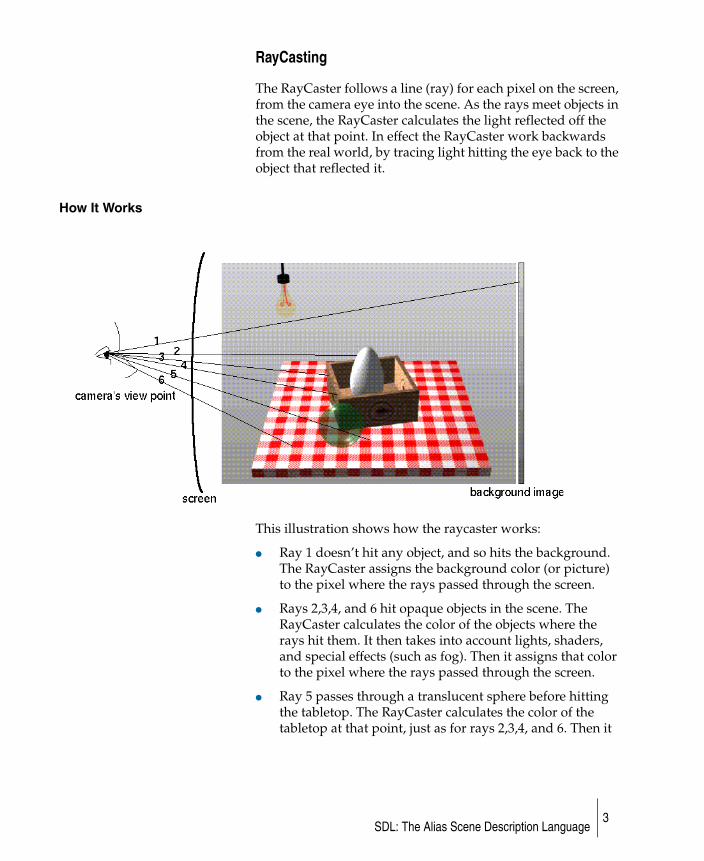
The RayCaster follows a line (ray) for each pixel on the screen, from the camera eye into the scene. As the rays meet objects in the scene, the RayCaster calculates the light reflected off the object at that point. In effect the RayCaster work backwards from the real world, by tracing light hitting the eye back to the object that reflected it.
How It Works
This illustration shows how the raycaster works:
● Ray 1 doesn’t hit any object, and so hits the background. The RayCaster assigns the background color (or picture) to the pixel where the rays passed through the screen.
● Rays 2,3,4, and 6 hit opaque objects in the scene. The RayCaster calculates the color of the objects where the rays hit them. It then takes into account lights, shaders, and special effects (such as fog). Then it assigns that color to the pixel where the rays passed through the screen.
● Ray 5 passes through a translucent sphere before hitting the tabletop. The RayCaster calculates the color of the tabletop at that point, just as for rays 2,3,4, and 6. Then it
3SDL: The Alias Scene Description Language
adds the amount of color the ray received from passing through the sphere. Finally it assigns that color to the pixel where the ray passed through the screen.
At each intersection between a ray and an object, the RayCaster combines the surface geometry, the lights in the scene, and the surface shading model to calculate the color for that spot. The shading model is a mathematical expression of the way the surface interacts with light. It is controlled by several parameters, such as surface color and shinyness, that can be constant over the surface (for solid colors), vary with U and V (for 2D textures), vary with XYZ (for solid textures), or vary with time (for animated colors and textures).
After calculating the color of the surface hit, the RayCaster takes into account atmospheric effects. That is, the medium through which the rays travel (for example, fog or water). These effects are controlled in the ENVIRONMENT section of SDL.
Once the RayCaster has completely processed a ray, taking into account surfaces and atmospheric effects, it has an RGB color value for the corresponding pixel on the screen. Depending on the options set when the RayCaster was run, it will use assign this color to the pixel, or calculate many rays per pixel and average their colors together for a “representative” color. This averaging is called anti-aliasing, and it helps to smooth out the blocky look of computer graphics. The amount of anti-aliasing is controlled in the DEFINITION section of SDL.
RayTracing
RayTracing is similar to RayCasting in many ways, but has one important difference — the ray of light doesn’t necessarily stop when it hits an opaque object. It can bounce off to another object and another and another, retracing and reflecting everything it sees in the scene. The StudioTools RayTracer follows as many bounces as you want.
RayTracing is more time-consuming than RayCasting, and for most scenes is not worth the extra time. However, it gives you the most realistic image possible. Because the ray is traced through multiple bounces, the RayTracer is able to produce effects the RayCaster cannot:
4SDL: The Alias Scene Description Language
● true reflections from reflective surfaces (to save rendering time, StudioTools lets you choose which objects in a scene will have reflections)
● true refraction through transparent surfaces
● true shadows from multiple light sources
● shadows cast through transparent objects
How It Works
The RayTracer follows the path of rays from the camera eye into the scene. Rays originating at the camera are the primary rays. As the primary rays intersect objects, they may reflect or refract according to simplified optical physics, and produce secondary rays. The secondary rays are followed in the same manner, and so on.
Each time a ray intersects an object, the RayTracer traces shadow rays from that point toward each lights set to cast shadows. If the shadow ray meets another surface before reaching the light, the point is shaded from the light.
The following illustration shows what would happen to ray 5 of the RayCasting example above, if it were rendered with RayTracing.
5SDL: The Alias Scene Description Language
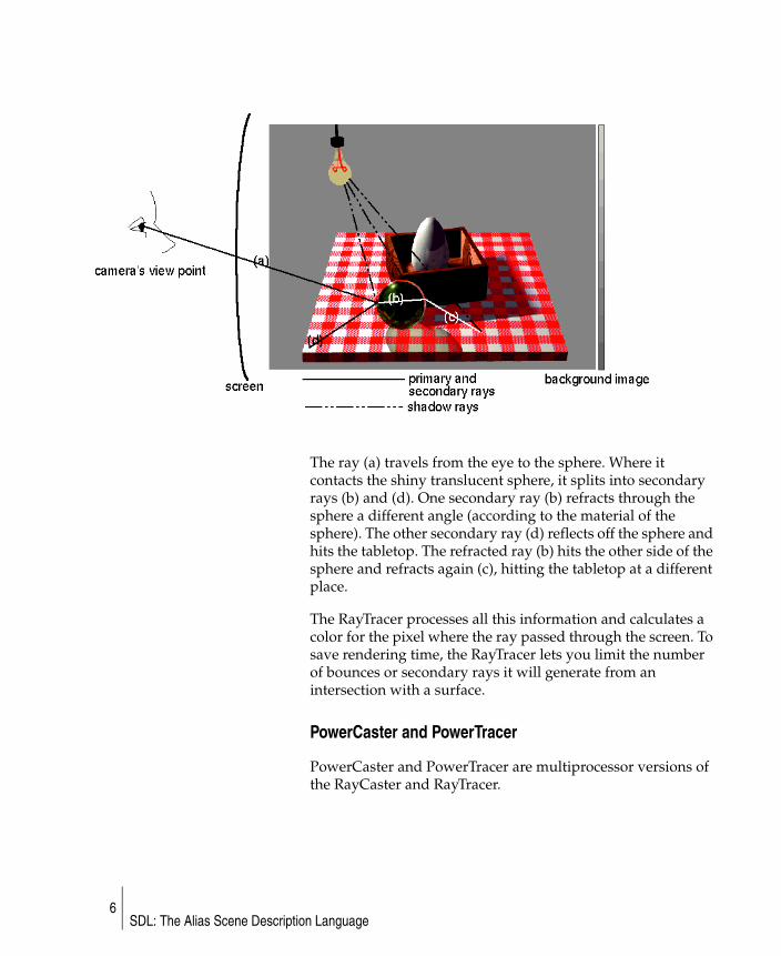
The ray (a) travels from the eye to the sphere. Where it contacts the shiny translucent sphere, it splits into secondary rays (b) and (d). One secondary ray (b) refracts through the sphere a different angle (according to the material of the sphere). The other secondary ray (d) reflects off the sphere and hits the tabletop. The refracted ray (b) hits the other side of the sphere and refracts again (c), hitting the tabletop at a different place.
The RayTracer processes all this information and calculates a color for the pixel where the ray passed through the screen. To save rendering time, the RayTracer lets you limit the number of bounces or secondary rays it will generate from an intersection with a surface.
PowerCaster and PowerTracer
PowerCaster and PowerTracer are multiprocessor versions of the RayCaster and RayTracer.
6SDL: The Alias Scene Description Language
C Pre-Processor "#include" Statements
Even a basic scene composed of cubes — each of which is represented by six patches — can look very imposing when printed out in a single SDL file.
To reduce the bulk of SDL files, you can use “#include” statements in the main SDL file and break the monolithic scene description into smaller, more manageable pieces. Before rendering, you use the C Pre-Processor to replace the “#include” statements with the smaller auxiliary files.
This method has several benefits when working with large SDL files by hand:
● allows you to isolate and separately maintain different types of scene description (for example, CV lists in one file, lights in another file, shaders in another file)
● makes it easier to edit files (smaller files load and display faster in an editor)
● allows you to replace redundant geometry (for example, two identical objects in a scene) with #include statements referencing the same file, while the different transformations for the objects remain in the main SDL file
Setting Up Include Files
Before beginning to create include files, consider creating a directory called include in the sdl directory. Putting SDL include files there reduces clutter and confusion.
To move parts of a master SDL file into smaller include files:
1 Copy the SDL text you want to include into a new file.
2 Candidates for replacement are long CV lists, lights, shaders, repetitive or complex geometry and transformations, and animation definitions.
3 Give a meaningful name to the new file containing the text to be included.
4 By convention, include files end with “.h”, but you can give them any name you want.
7SDL: The Alias Scene Description Language
5 In the master SDL file, replace the text you just copied with a line beginning with #include, followed by a space and the quoted path to the file to be included. For example: #include “/h/frank/includes/geom.h”
6 Repeat for each section of SDL text you want to move into an include file.
Recreating the SDL File for Rendering
Before you can render SDL files with #include statements, you must expand them by replacing the #include statements in the master SDL file with the text contained in the corresponding include files. To do this, you will run the master SDL file through the C Pre-Processor, cpp.
The StudioTools interactive software and the renderit script both run cpp on SDL files automatically.
To manually expand an SDL file for rendering:
1 At a shell prompt, type
2 /lib/cpp -C -P sdl/masterSDLfile temp
3 Where masterSDLfile is the name of the SDL file with the include statements. This runs the master SDL file through cpp and creates a new file called temp, which is the result of replacing the “#include” statements.
4 At the prompt, type
5 renderer temp
6 This runs the renderer on the recreated file.
8SDL: The Alias Scene Description Language

The Rendering Pipeline
In the pre-processing phase, the RayCaster:
1 Takes face, patch, and polygon statements from the SDL file.
2 Transforms the control vertices of each object according to the SDL hierarchy of transformations.
3 Converts the geometry into triangles.
4 The number of triangles depends on the tessellation control settings. The vertex of each triangle stores surface U and V parameters, tangent vectors, surface normal, and position in world space.
5 Applies the perspective viewing transformation, which includes the camera location, viewpoint, field of view, and twist.
6 This step converts the triangles from world space to perspective (screen) space.
7 The triangles are “scanned out” to the triangle buffer (each pixel inside the two-dimensional boundary of the screen space triangle is identified).
In the rendering phase, the RayCaster loops through each pixel of the new image and calculates:
1 The light reflected toward the camera by each surface.
2 U and V parameter values, tangent vectors, surface normal, and position for each intersection point with a triangle (calculated by interpolating from the information on the intersected triangle in the triangle buffer).
3 Color and transparency values for the intersected triangle(s) based on the geometry of the intersecting point, the lights in the scene, and the surface shading model.
4 Final color (RGB) and transparency (alpha) of the pixel based on the colors and transparencies of the intersected triangle(s).
The final step of combining all the intersected triangles into a final color is complex.
9SDL: The Alias Scene Description Language
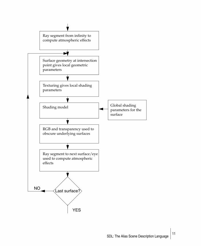
If the ray intersects more than one triangle, the list of intersections is sorted by distance from the camera and processed from back to front. The renderer builds the final color and transparency by combining the colors and transparencies of each triangle, along with the atmospheric effects between the triangles. See the Procedural Textures and Natural Phenomena (page 483) section of the SDL Reference Manual for more information on how these colors are calculated and combined.
This illustration shows the complex process by which the renderer combines the colors of the intersected triangles. It does not show the additional complexities introduced by motion blur.
10SDL: The Alias Scene Description Language
Ray segment from infinity to compute atmospheric effects
Surface geometry at intersection point gives local geometric parameters
Texturing gives local shading parameters
Shading model
RGB and transparency used to obscure underlying surfaces
Ray segment to next surface/eye used to compute atmospheric effects
Global shading parameters for the surface
Last surface?
YES
NO
11SDL: The Alias Scene Description Language
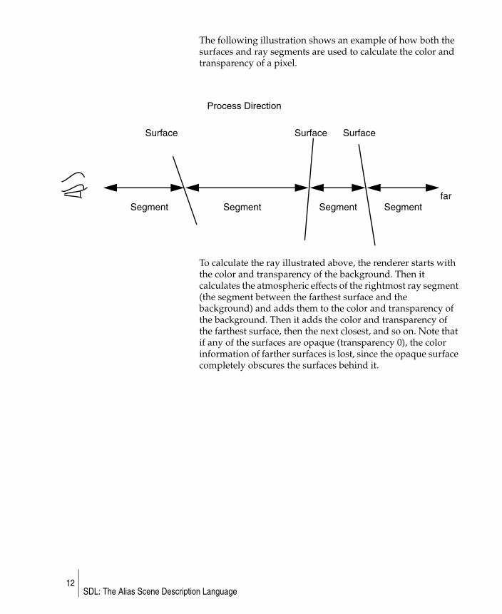
The following illustration shows an example of how both the surfaces and ray segments are used to calculate the color and transparency of a pixel.
To calculate the ray illustrated above, the renderer starts with the color and transparency of the background. Then it calculates the atmospheric effects of the rightmost ray segment (the segment between the farthest surface and the background) and adds them to the color and transparency of the background. Then it adds the color and transparency of the farthest surface, then the next closest, and so on. Note that if any of the surfaces are opaque (transparency 0), the color information of farther surfaces is lost, since the opaque surface completely obscures the surfaces behind it.
Process Direction
Segment
Surface Surface Surface
Segment Segment Segmentfar
12SDL: The Alias Scene Description Language

Command Line Options
Any options you give the renderer on the command line override internal variables in the SDL file. These options allow you to change the behavior of the renderer without having to edit the SDL file.
Usage
To use the command line options
1 Use the cd command to move to your project directory (for example, cd user_data/demo).
2 Enter the command for the renderer, followed by any options (see below), and the name of the SDL file (for example, renderer -s10 sdl/animation_1).
Options
renderer|raytracer[-H] [-an] [-bn] [-en] [-f script] [-gn][-hn] [-m filename] [-p filename] [-d filename] [-C color_map_filename] [-c quantized_output_file] [-j] [-k] [-Kn] [-on] [-O][-qn][-P][-sn] [-Sn] [-Bn] [-En] [-rn] [-tn] [-wn] [-Wn] [-xn] [-yn] [-Yn] [-zn] [-Zn] [filename]
-an Use the integer n as the aalevel.
-tn Use the integer n as the aathreshold.
-sn Use the float n as the starting frame number.
-bn Use the float n as the by frame number.
-en Use the float n as the ending frame number.
-Sn Use the integer n as the start extension.
-Bn Use the integer n as the by extension.
-En Use the integer n as the size extension.
-fstring invoke the program string after each frame.
-gn Use the float n as the gamma correction value.
-mstring Produce a matte file and Use string as the filename.
-pstring Use string as the pix filename.
-dstring Use string as the depth file name.
13SDL: The Alias Scene Description Language
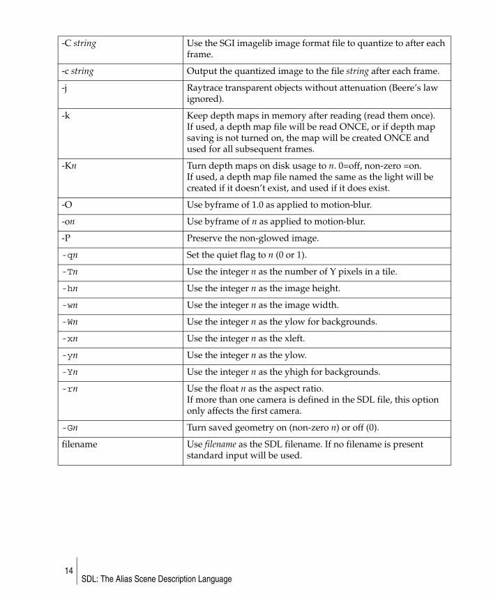
-C string Use the SGI imagelib image format file to quantize to after each frame.
-c string Output the quantized image to the file string after each frame.
-j Raytrace transparent objects without attenuation (Beere’s law ignored).
-k Keep depth maps in memory after reading (read them once).If used, a depth map file will be read ONCE, or if depth map saving is not turned on, the map will be created ONCE and used for all subsequent frames.
-Kn Turn depth maps on disk usage to n. 0=off, non-zero =on.If used, a depth map file named the same as the light will be created if it doesn’t exist, and used if it does exist.
-O Use byframe of 1.0 as applied to motion-blur.
-on Use byframe of n as applied to motion-blur.
-P Preserve the non-glowed image.
-qn Set the quiet flag to n (0 or 1).
-Tn Use the integer n as the number of Y pixels in a tile.
-hn Use the integer n as the image height.
-wn Use the integer n as the image width.
-Wn Use the integer n as the ylow for backgrounds.
-xn Use the integer n as the xleft.
-yn Use the integer n as the ylow.
-Yn Use the integer n as the yhigh for backgrounds.
-rn Use the float n as the aspect ratio.If more than one camera is defined in the SDL file, this option only affects the first camera.
-Gn Turn saved geometry on (non-zero n) or off (0).
filename Use filename as the SDL filename. If no filename is present standard input will be used.
14SDL: The Alias Scene Description Language
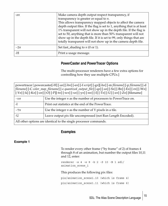
PowerCaster and PowerTracer Options
The multi-processor renderers have a few extra options for controlling how they use multiple CPUs.]
Examples
Example 1
To render every other frame (“by frame” of 2) of frames 4 through 8 of an animation, but number the output files 10,11 and 12, enter:
renderer -s 4 -e 8 -b 2 -S 10 -B 1 sdl/animation_scene_1
This produces the following pix files:
pix/animation_scene1.10 (which is frame 4)
pix/animation_scene1.11 (which is frame 6)
-zn Make camera depth output respect transparency, if transparency is greater or equal to n.This allows transparency mapped objects to affect the camera depth output files. If the flag is set to 1, anything that is at least 1% transparent will not show up in the depth file. If the flag is set to 50, anything that is more than 50% transparent will not show up in the depth file. If it is set to 99, only things that are totally transparent will not show up in the camera depth file.
-Zn Set fast_shading to n (0 or 1).
-H Print a usage message.
powertracer|powercaster[-H] [-an] [-bn] [-en] [-f script] [-gn][-hn] [-m filename] [-p filename] [-d filename] [-C color_map_filename] [-c quantized_output_file] [-qn] [-sn] [-Sn] [-Bn] [-En] [-rn] [-Wn] [-Yn] [-k] [-Kn] [-on] [-O] [-P][-tn] [-wn] [-xn] [-yn] [-nn] [-I] [-Tn] [-U] [-zn] [-Zn] [filename]
-nn Use the integer n as the number of processors to PowerTrace on.
-I Print out statistics at the end of the PowerTrace.
-Tn Use the integer n as the number of Y pixels in a tile.
-U Leave output pix file uncompressed (not Run Length Encoded).
All other options are identical to the single processor commands.
15SDL: The Alias Scene Description Language
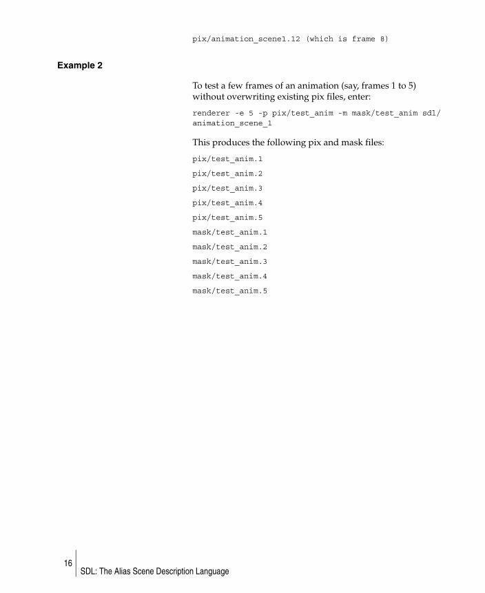
pix/animation_scene1.12 (which is frame 8)
Example 2
To test a few frames of an animation (say, frames 1 to 5) without overwriting existing pix files, enter:
renderer -e 5 -p pix/test_anim -m mask/test_anim sdl/animation_scene_1
This produces the following pix and mask files:
pix/test_anim.1
pix/test_anim.2
pix/test_anim.3
pix/test_anim.4
pix/test_anim.5
mask/test_anim.1
mask/test_anim.2
mask/test_anim.3
mask/test_anim.4
mask/test_anim.5
16SDL: The Alias Scene Description Language

Inserting comments in SDL
To insert comments in an SDL file, enclose the line or lines with a “C style” slash-asterisk pair:
/* comment */
or
/*
comment
comment
comment
*/
You cannot nest comments.
The numeric sign (#) followed by a blank space is not a comment.
17SDL: The Alias Scene Description Language

18SDL: The Alias Scene Description Language

Scene Description Language Reference
19
Designing SDL
The Scene Description Language is intended to describe a scene. It is not meant for interaction. When Alias Systems created SDL, the most important consideration was its ability to clearly and succinctly describe a scene. This includes sufficient scope to describe all aspects of a scene.
In addition, SDL had to be
● practical in normal and extraordinary usage;
● extensible to evolve as new features are added in the future;
● flexible to cope with the differing needs of ID and video animation;
● intuitive for first time and casual users;
● rich with options for skilled and demanding users;
● internally consistent for ease of teaching and documentation;
● and consistent with the interactive package to avoid confusion.
The above considerations argued for a language rich in nouns and adjectives, with fewer verbs. In terms of computer language design, that means many data types with many optional modifiers and relatively few operations. The bulk of this document, therefore, deals with data.
20
Notation
We have tried to keep the vocabulary in this document strictly defined. For example, each data type has a unique name. That name is not used with any other meaning in this document.
This document does not include a glossary, since any description of the terms used would simply repeat the description of the language feature. Please check the table of contents for any term which is unfamiliar, since most terms important to SDL have their own section.
Three-dimensional coordinates and directions are specified using the x,y,z system, corresponding to the system used by the modeler.
Reserved words are printed in bold.
21
Layout
There are five sections in this part of the manual:
● SDL File Roadmap
● Using Data Items
● System Defined Variables and System Defined Constants
● Expressions and Functions
22

New Keyword Equivalents
Starting with version 7, some keywords have shorter “nicknames”, allowing smaller file sizes and easier typing. For example you can now use cl instead of cluster, inst instead of instance, pc instead of parameter_curve, and so on.
23
SDL File Roadmap
This is a roadmap of an SDL file. Every item that can be included is shown here, but if your model does not use any of these features they should not appear in the SDL file.
An SDL file is divided into three sections: DEFINITION, ENVIRONMENT, and MODEL. The sections are preceded by section titles, which are entered on a line in all caps with no punctuation.
The camera is listed last in this example layout, but it may appear anywhere in the MODEL section, and there can be more than one camera. Note that the camera object contains the mask, depth_file, and pix file name specifications.
DEFINITION Section
● system variables (for example, aalevel, frame range, ray tracing levels)
● animation curves (motion paths and timing curves)
● camera view variable(s)
● light definitions
● shader and texture definitions
● trim curve definitions
● patch and face definitions (note: text is now represented as faces)
ENVIRONMENT Section
● background type (file, ramp, color, procedural, none)
● fog specification
MODEL Section
● instances and transformations (the building blocks of a model)
● camera(s) (contains output image file name)
24
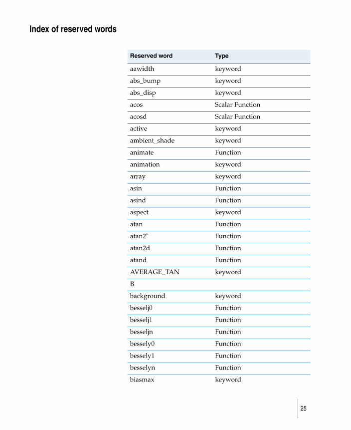
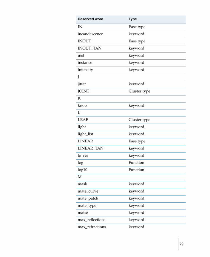
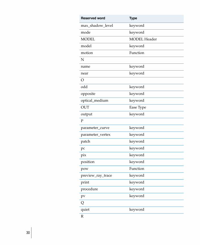
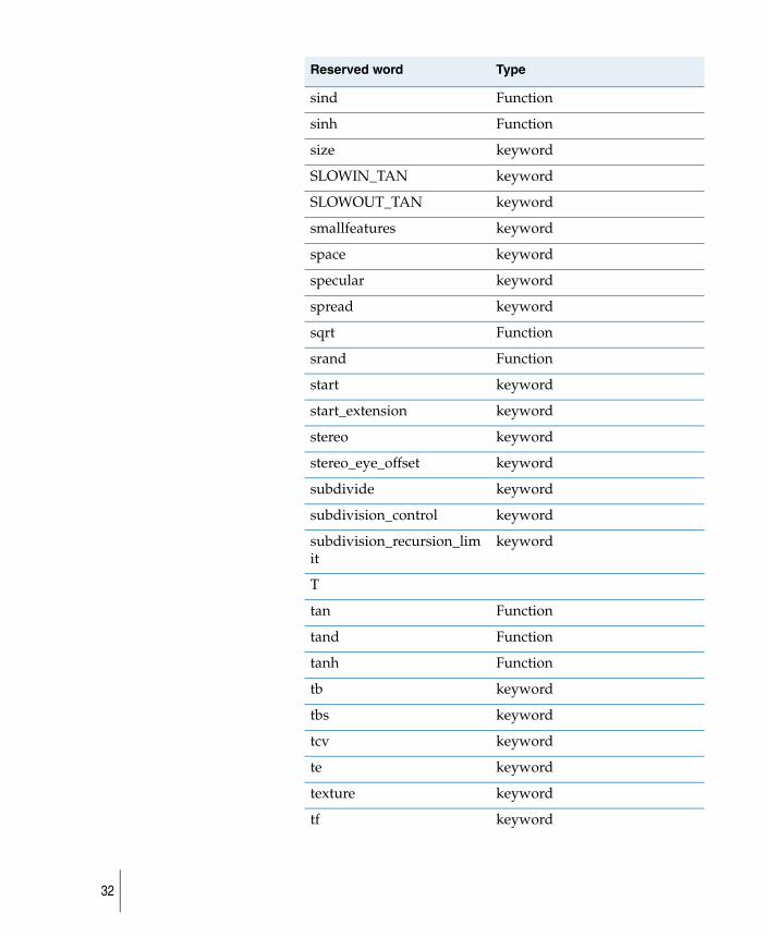
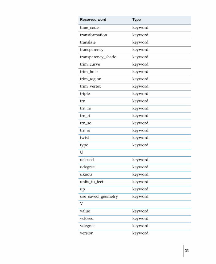
Index of reserved words
Reserved word Type
aawidth keyword
abs_bump keyword
abs_disp keyword
acos Scalar Function
acosd Scalar Function
active keyword
ambient_shade keyword
animate Function
animation keyword
array keyword
asin Function
asind Function
aspect keyword
atan Function
atan2" Function
atan2d Function
atand Function
AVERAGE_TAN keyword
B
background keyword
besselj0 Function
besselj1 Function
besseljn Function
bessely0 Function
bessely1 Function
besselyn Function
biasmax keyword
25
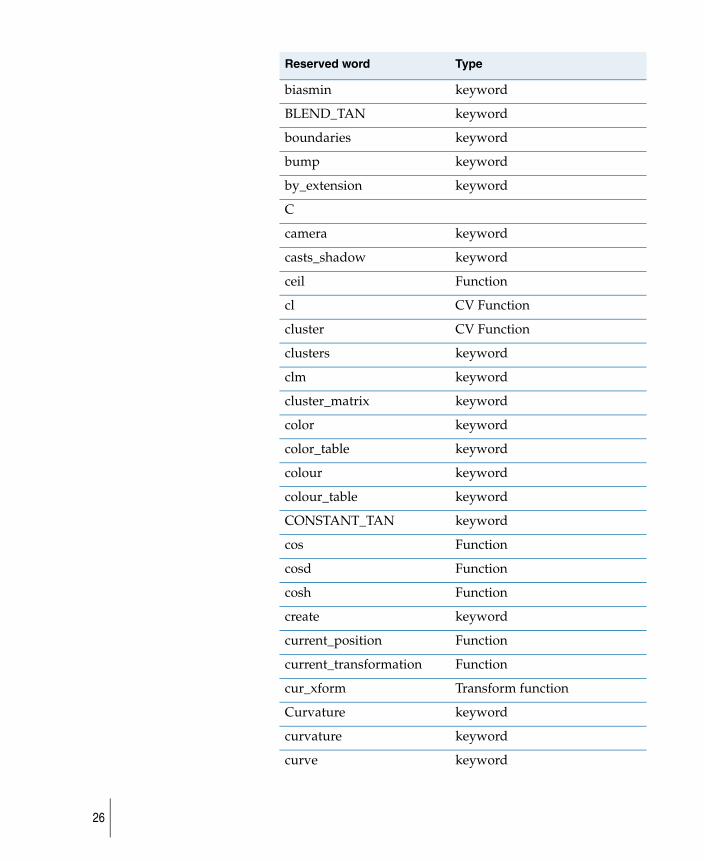
biasmin keyword
BLEND_TAN keyword
boundaries keyword
bump keyword
by_extension keyword
C
camera keyword
casts_shadow keyword
ceil Function
cl CV Function
cluster CV Function
clusters keyword
clm keyword
cluster_matrix keyword
color keyword
color_table keyword
colour keyword
colour_table keyword
CONSTANT_TAN keyword
cos Function
cosd Function
cosh Function
create keyword
current_position Function
current_transformation Function
cur_xform Transform function
Curvature keyword
curvature keyword
curve keyword
Reserved word Type
26
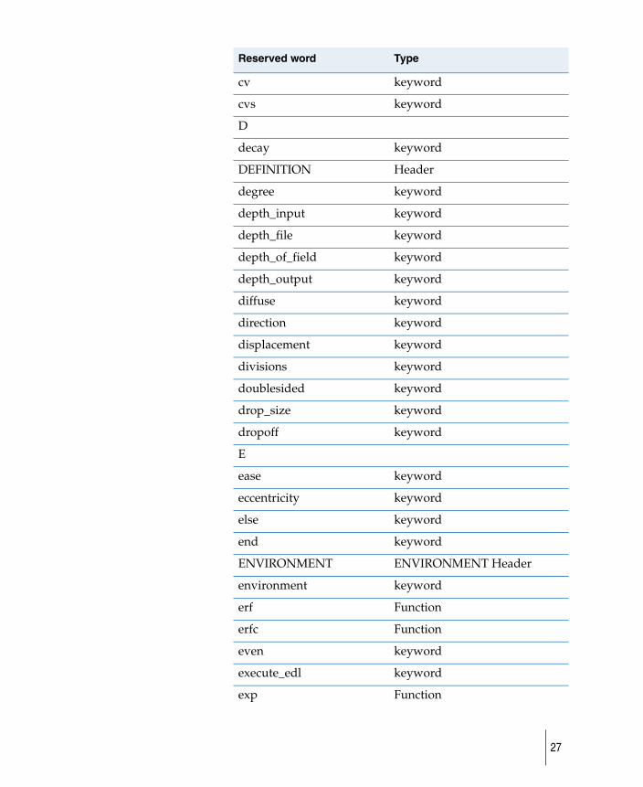
cv keyword
cvs keyword
D
decay keyword
DEFINITION Header
degree keyword
depth_input keyword
depth_file keyword
depth_of_field keyword
depth_output keyword
diffuse keyword
direction keyword
displacement keyword
divisions keyword
doublesided keyword
drop_size keyword
dropoff keyword
E
ease keyword
eccentricity keyword
else keyword
end keyword
ENVIRONMENT ENVIRONMENT Header
environment keyword
erf Function
erfc Function
even keyword
execute_edl keyword
exp Function
Reserved word Type
27
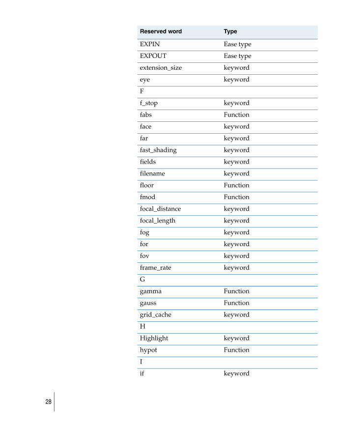
EXPIN Ease type
EXPOUT Ease type
extension_size keyword
eye keyword
F
f_stop keyword
fabs Function
face keyword
far keyword
fast_shading keyword
fields keyword
filename keyword
floor Function
fmod Function
focal_distance keyword
focal_length keyword
fog keyword
for keyword
fov keyword
frame_rate keyword
G
gamma Function
gauss Function
grid_cache keyword
H
Highlight keyword
hypot Function
I
if keyword
Reserved word Type
28
IN Ease type
incandescence keyword
INOUT Ease type
INOUT_TAN keyword
inst keyword
instance keyword
intensity keyword
J
jitter keyword
JOINT Cluster type
K
knots keyword
L
LEAF Cluster type
light keyword
light_list keyword
LINEAR Ease type
LINEAR_TAN keyword
lo_res keyword
log Function
log10 Function
M
mask keyword
mate_curve keyword
mate_patch keyword
mate_type keyword
matte keyword
max_reflections keyword
max_refractions keyword
Reserved word Type
29
max_shadow_level keyword
mode keyword
MODEL MODEL Header
model keyword
motion Function
N
name keyword
near keyword
O
odd keyword
opposite keyword
optical_medium keyword
OUT Ease Type
output keyword
P
parameter_curve keyword
parameter_vertex keyword
patch keyword
pc keyword
pix keyword
position keyword
pow Function
preview_ray_trace keyword
print keyword
procedure keyword
pv keyword
Q
quiet keyword
R
Reserved word Type
30

ramp keyword
rand Function
raycast Mode Type
record_device_number keyword
reflection keyword
reflection_limit keyword
reflectivity keyword
refraction_limit keyword
refractive_index keyword
resolution keyword
respect_reflection_map keyword
rot keyword
rotate keyword
S
scalar keyword
scale keyword
sclr keyword
shader keyword
shadow keyword
shadow_level_limit keyword
shadow_output keyword
shadow_volume keyword
shadowmult keyword
shadowoffset keyword
shared_edge keyword
shine_along keyword
shinyness keyword
sign Function
sin Function
Reserved word Type
31
sind Function
sinh Function
size keyword
SLOWIN_TAN keyword
SLOWOUT_TAN keyword
smallfeatures keyword
space keyword
specular keyword
spread keyword
sqrt Function
srand Function
start keyword
start_extension keyword
stereo keyword
stereo_eye_offset keyword
subdivide keyword
subdivision_control keyword
subdivision_recursion_limit
keyword
T
tan Function
tand Function
tanh Function
tb keyword
tbs keyword
tcv keyword
te keyword
texture keyword
tf keyword
Reserved word Type
32
time_code keyword
transformation keyword
translate keyword
transparency keyword
transparency_shade keyword
trim_curve keyword
trim_hole keyword
trim_region keyword
trim_vertex keyword
triple keyword
trn keyword
trn_ro keyword
trn_ri keyword
trn_so keyword
trn_si keyword
twist keyword
type keyword
U
uclosed keyword
udegree keyword
uknots keyword
units_to_feet keyword
up keyword
use_saved_geometry keyword
V
value keyword
vclosed keyword
vdegree keyword
version keyword
Reserved word Type
33
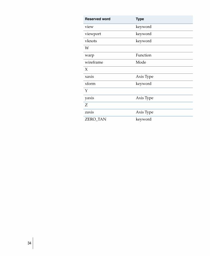
view keyword
viewport keyword
vknots keyword
W
warp Function
wireframe Mode
X
xaxis Axis Type
xform keyword
Y
yaxis Axis Type
Z
zaxis Axis Type
ZERO_TAN keyword
Reserved word Type
34
MODEL SectionThe MODEL section describes the instances of the objects that were defined in the DEFINITION section, along with information for position, orientation, relationships between objects, and behavior over time. The MODEL section contains statements about data items (for creating, inspecting, and transforming), and control statements (for conditional execution and looping).
The MODEL section is similar to the old GEOMETRY section, but uses objects defined in the DEFINITION section.
The MODEL section begins with the word MODEL in all caps on a separate line with no punctuation. The section ends when the SDL file ends.
The following statements are described in this section:
● <assignment>
● for
● if
● instance
● <literal>
● rotate
● scale
● <(null)>
● translate
● translate_pivot
● translate_ripivot
● translate_ropivot
● translate_sipivot
● translate_sopivot
● { }
35
assignment
Syntax:
<left hand side> = <right hand side> ;
Purpose:
This assigns the value of the item on the right to the item on the left. The item on the right is not modified or otherwise effected in any way. The <left hand side> may be a variable name, an array name, or an array element reference. The <right hand side> may be a literal, a variable reference, an array name, or an array element reference or a function. However, only certain of the possible combinations are valid. The following rules determine the validity.
If the <left hand side> is an array element reference, then any of the <right hand side> possibilities may be used.
If the <left hand side> is a variable name, the <right hand side> may be a literal, a variable reference, or an array element reference or a function, provided that the data types of the <left hand side> and the <right hand side> are the same.
Example:
switch = FALSE;
bunch[1] = some_var;
36
for
Syntax:
for ( <initial statement>; <condition> ; <iteration statement>; ) <body statement>
Purpose:
The for statement provides a means of iterating loops of statements. The structure of the for statement is considerably more powerful than that provided by most languages. The particulars of it are different than “C”, but have a similar flavor.
The <initial statement> is any statement valid in the MODEL section. Typically it will be an assignment, but it is not limited to that. (It could be a (null) grouping or even a nested for statement.) An <initial statement> must be specified.
The <condition> is just an expression interpreted as a truth value. An expression is considered true if its value is non-zero, and false if its value is zero. If <condition> is true, then the <body statement> will be executed. If <condition> is false, then control immediately passes to the statement following the for statement. A <condition> must be specified.
The <iteration statement> is any statement valid in the MODEL section. An <iteration statement> must be specified. The <body statement> is any statement valid in the MODEL section. A <body statement> must be specified.
All the elements of a for statement are always required. The parentheses and semi-colon are part of the syntax, and required. The end of a for statement is marked by the end of the <body statement>.
There are four parts to the execution of a for statement. First, the <initial statement> is executed. Second, the <condition> is tested. The result of this is either continued execution or the end of the for statement. Third, if execution is to be continued, the <body statement> is executed. Fourth, the <iteration statement> is executed. Following this, control reverts to the second step, testing the <condition>, and proceeds from that
37
point. Execution continues in this way until the <condition> evaluates to false.
Example:
for ( x=0; x < 10; x = x+1;) print("digit =", x );
38
{ }
Syntax:
{ <statement> <statement> … <statement> }
Purpose:
An arbitrary number of MODEL section statements may be grouped together through the use of the brace bracket characters, { and }. The start of the group is marked by the opening brace, {. The end of the group is marked by the closing brace, }. All statements between the braces are treated as though they were one single statement. Transformation statements (rotate, translate and scale) only have effect within the group. Instances and literals create objects in the scene. Assignments effect the value of variables, which retain their values across the boundaries of the group. All other statements behave in their normal manner. Groups may be nested to any degree.
Groups are useful for two purposes. First, groups allow hierarchies of objects and transformations to be constructed. When used in this sense, they are identical to the groups found in the interactive package. Second, groups are useful for extending the range of effect of if statements and for statements. This usage of groups is not presently available in the interactive package. It is, however, vary similar to syntactic constructs in “C” and other programming languages.
39
if
Syntax:
if ( <condition> ) <true statement> else <false statement>
or
if ( <condition> ) <true statement>
Purpose:
The if statement is used to conditionally execute statements. The <condition> is just an expression interpreted as a truth value. An expression is considered true if its value is non-zero, and false if its value is zero. If <condition> is true, the <true statement> is executed. Otherwise, the <false statement> is executed. The if statement can be abbreviated by omitting the else and the <false statement>.
In its abbreviated form, the if statement will execute the <true statement> if the <condition> is true, and pass on to the next statement if it is false. <true statement> and <false statement> may be any statement valid in the MODEL section (including if statements and {} groupings). The end of an if statement is marked by the end of the <false statement> (or by the end of the <true statement> in the abbreviated form).
Example:
if (frame > 1) begun = TRUE;
40
instance
Syntax:
instance <object reference> ();
or
inst <object reference> ();
Purpose:
The instance statement creates an instance of an object. The <object reference> may be either a variable reference or an array element reference. In either case, an object is created from the data item. The data item being referenced must be of an appropriate type (that is, Light Data Type, Patch Data Type, Face Data Type, or Camera Data Type). If the <object reference> is a variable reference, then the type check is performed at parse time, otherwise it is performed at instancing time. If an improper data type is given, a warning message is issued and execution continues with the instance ignored. The effect of an instance is the same as if a literal of the same type and having the component values of the <object reference> were used instead.
The end of an instance statement is marked by a semi-colon.
Note that inst and instance keywords can be used interchangeably.
Example:
instance sphere_patch();
41
literal
Syntax:
The syntax of a literal definition varies, depending upon the data type of the literal being defined. The reader is referred to the detailed description of the data types for the exact syntax of each. Note that only literals of “objects” may be used. That is, only Light Data Type, Patch Data Type, Face Data Type, and Camera Data Type are valid. If an improper data type is given, a warning is issued and execution continues with the literal ignored.
Purpose:
The specification of a literal object places that object in the scene at the location and with the size and orientation determined by the current transform matrix. The end of a literal statement is marked by a semi-colon.
42
(null)
Syntax:
;
Purpose:
The null statement (a lone semi-colon) is a valid and well-defined statement that does nothing. It is useful in those situations where a statement is required, but no action is desired. For example, a for statement with an empty initial statement could be written as
for ( ; x < 5; x = x+1; ) print("count =", x );
43
Syntax:
print ( "string", <scalar | triple> ) ;
or
print ( "string" ) ;
Purpose:
This statement prints a string and the value of a scalar, or just a string. The string is required, although it may be empty.
print may be used by itself, for example
print ("This just prints a comment");
Alternately, print may be used as a function within some larger construct. When used in this way, print passes the value of the variable through as though the print were not there at all. For example,
x = print ("x = ", a );
results in x being assigned the value of variable a. If only a string is given (no variable), the passed through value is scalar(0). Thus,
x = print ("This is just a comment");
is equivalent to assigning the scalar value 0 to variable x. The end of a print statement is marked by a semicolon.
If the item being printed is a triple, the return value of the print statement is also a triple.
Example:
print("a thing", thing);
44
rotate
Syntax:
rotate ( <axis index>, <scalar> ) ;
or
rot ( <axis index>, <scalar> ) ;
Purpose:
Rotations are performed about an axis. The <axis index> specifies which axis to rotate about. The <axis index> is just a scalar, interpreted as an integer. It must have a value of 0, 1 or 2, where a value of 0 indicates rotation about the x axis, 1 indicates rotation about the y axis, and 2 indicates rotation about the z axis. Three system defined constants are provided (xaxis, yaxis, and zaxis) for convenience in specifying the <axis index>. The <scalar> specifies the amount of rotation (measured in degrees). The order of application for rotate statements is important. A rotate statement for the x axis followed by one for the z axis does not have the same effect as the reverse order of application. The end of a rotate statement is marked by a semi-colon.
Note that rot and rotate keywords can be used interchangeably.
Example:
rotate(zaxis, 45);
45
translate
Syntax:
translate <triple> ;
or
trn <triple> ;
Purpose:
The <triple> indicates the direction in which the subsequent geometry is moved. The end of a translate statement is marked by a semi-colon.
Note that trn and translate keywords can be used interchangeably.
Example:
translate (0,15,0.2);
46
scale
Syntax:
scale <triple> ;
Purpose:
The components of the <triple> multiply the coordinate values of points for each of the x, y and z directions with respect to the origin. A scale of (1,1,1) has no effect on the objects, while a scale of (1, 1, 1.5) creates a 50 percent increase in the z dimension. Note that a scale of (0, 0, 0) is an error; it is ignored by the renderer, and a warning message is given. The end of a scale statement is marked by a semi-colon.
Example:
scale (1,1,0.2);
47
translate_pivot
Syntax:
translate_pivot <triple>;
Purpose:
The <triple> indicates the direction in which the subsequent geometry is moved. The end of a translate_pivot statement is marked by a semi-colon. translate_pivot is similar to translate, except translations used in translate_pivot do not get used in cluster matrix building.
Example:translate_pivot (0.1, 3.0, 2.5);
48
translate_ripivot
Syntax:
translate_ripivot <triple>;
or
trn_ri <triple>;
Purpose:
The <triple> indicates the direction in which the subsequent geometry is moved. The end of a translate_ripivot statement is marked by a semi-colon. translate_ripivot is similar to translate, except translations used in translate_ripivot do not get used in cluster matrix building and only affects rotation in.
Note that trn_ri and translate_ripivot can be used interchangeably.
Example:
translate_ripivot (0.1, 3.0, 2.5);
49

translate_ropivot
Syntax:
translate_ropivot <triple>;
or
trn_ro <triple>;
Purpose:
The <triple> indicates the direction in which the subsequent geometry is moved. The end of a translate_ropivot statement is marked by a semi-colon. translate_ropivot is similar to translate, except translations used in translate_ropivot do not get used in cluster matrix building and only affects rotation out.
Note that trn_ri and translate_ripivot can be used interchangeably.
Example:
translate_ropivot (0.1, 3.0, 2.5);
50
translate_sipivot
Syntax:
translate_sipivot <triple>;
or
trn_si <triple>;
Purpose:
The <triple> indicates the direction in which the subsequent geometry is moved. The end of a translate_sipivot statement is marked by a semi-colon. translate_sipivot is similar to scale, except translations used in translate_sipivot do not get used in cluster matrix building and only affects scale in.
Note that trn_si and translate_sipivot can be used interchangeably.
Example:
translate_sipivot (0.1, 3.0, 2.5);
51
translate_sopivot
Syntax:
translate_sopivot <triple>;
or
trn_so <triple>;
Purpose:
The <triple> indicates the direction in which the subsequent geometry is moved. The end of a translate_sopivot statement is marked by a semi-colon. translate_sopivot is similar to scale, except translations used in translate_sopivot do not get used in cluster matrix building and only affects rotation out.
Note that trn_si and translate_sipivot can be used interchangeably.
Example:
translate_sopivot (0.1, 3.0, 2.5);
52
DEFINITION SectionThe DEFINITION section contains definitions of all the entities that will be “instanced” later in the MODEL section, similar to declaring variables before using them in traditional programming languages.
The DEFINITION section is the place for definitions of:
● system variables (for example, aalevel, frame range, ray tracing levels)
● animation curves (motion paths and timing curves)
● camera view(s)
● lights
● shaders and textures
● trim curves
● patches and faces
The background and atmospheric effects are defined in the ENVIRONMENT section.
The DEFINITION section begins with the word DEFINITION in all caps on a separate line with no punctuation. The section ends where the next section begins.
The DEFINITION section contains declarations of data items (see below for data types and syntax). The order in which items are defined is significant: declarations can only refer to variables that were defined previously in the text file.
A large percentage of the SDL file is taken up by the DEFINITION section. See the section on the C Pre-Processor and #include statements for ways to reduce the bulk of the SDL file and increase clarity.
Render Parameters
The renderer is controlled by parameters in the SDL file. You can override many of the parameters in the SDL file with
53
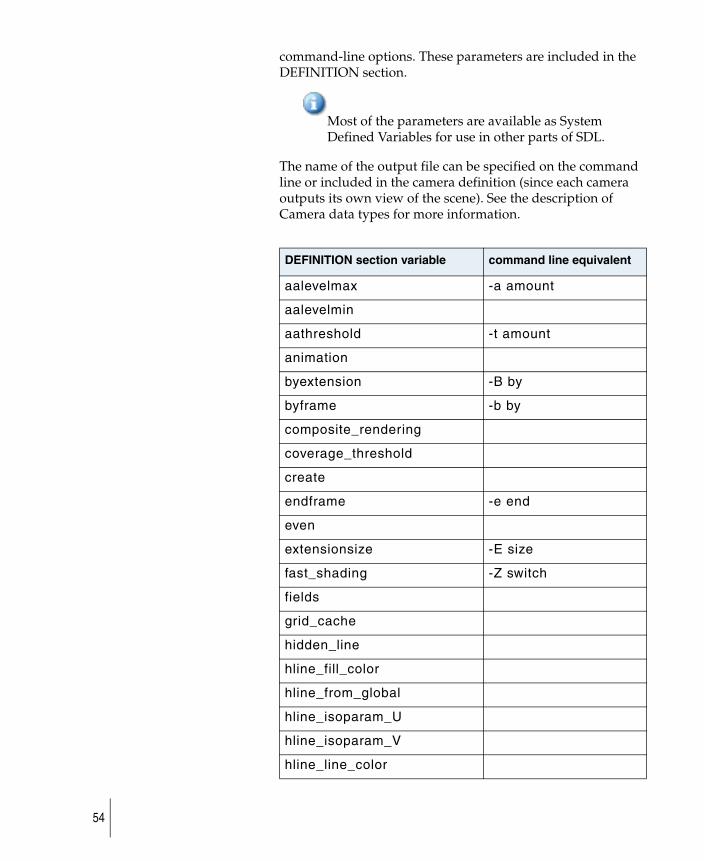
command-line options. These parameters are included in the DEFINITION section.
Most of the parameters are available as System Defined Variables for use in other parts of SDL.
The name of the output file can be specified on the command line or included in the camera definition (since each camera outputs its own view of the scene). See the description of Camera data types for more information.
DEFINITION section variable command line equivalent
aalevelmax -a amount
aalevelmin
aathreshold -t amount
animation
byextension -B by
byframe -b by
composite_rendering
coverage_threshold
create
endframe -e end
even
extensionsize -E size
fast_shading -Z switch
fields
grid_cache
hidden_line
hline_fill_color
hline_from_global
hline_isoparam_U
hline_isoparam_V
hline_line_color
54
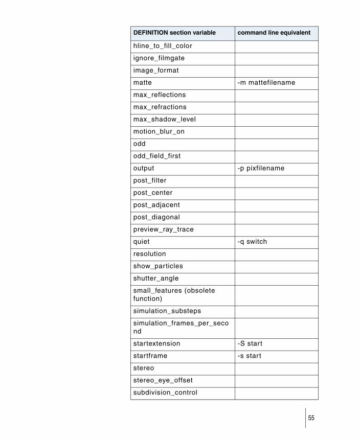
hline_to_fill_color
ignore_filmgate
image_format
matte -m mattefilename
max_reflections
max_refractions
max_shadow_level
motion_blur_on
odd
odd_field_first
output -p pixfilename
post_filter
post_center
post_adjacent
post_diagonal
preview_ray_trace
quiet -q switch
resolution
show_particles
shutter_angle
small_features (obsolete function)
simulation_substeps
simulation_frames_per_second
startextension -S start
startframe -s start
stereo
stereo_eye_offset
subdivision_control
DEFINITION section variable command line equivalent
55
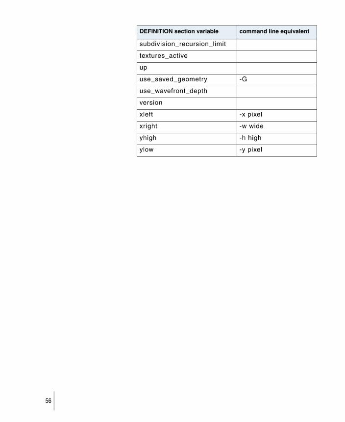
subdivision_recursion_limit
textures_active
up
use_saved_geometry -G
use_wavefront_depth
version
xleft -x pixel
xright -w wide
yhigh -h high
ylow -y pixel
DEFINITION section variable command line equivalent
56
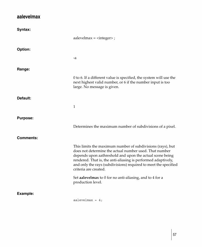
aalevelmax
Syntax:
aalevelmax = <integer> ;
Option:
-a
Range:
0 to 6. If a different value is specified, the system will use the next highest valid number, or 6 if the number input is too large. No message is given.
Default:
1
Purpose:
Determines the maximum number of subdivisions of a pixel.
Comments:
This limits the maximum number of subdivisions (rays), but does not determine the actual number used. That number depends upon aathreshold and upon the actual scene being rendered. That is, the anti-aliasing is performed adaptively, and only the rays (subdivisions) required to meet the specified criteria are created.
Set aalevelmax to 0 for no anti-aliasing, and to 4 for a production level.
Example:
aalevelmax = 4;
57
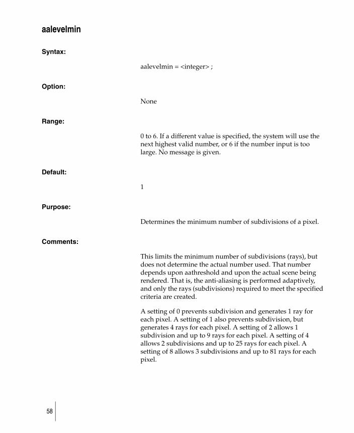
aalevelmin
Syntax:
aalevelmin = <integer> ;
Option:
None
Range:
0 to 6. If a different value is specified, the system will use the next highest valid number, or 6 if the number input is too large. No message is given.
Default:
1
Purpose:
Determines the minimum number of subdivisions of a pixel.
Comments:
This limits the minimum number of subdivisions (rays), but does not determine the actual number used. That number depends upon aathreshold and upon the actual scene being rendered. That is, the anti-aliasing is performed adaptively, and only the rays (subdivisions) required to meet the specified criteria are created.
A setting of 0 prevents subdivision and generates 1 ray for each pixel. A setting of 1 also prevents subdivision, but generates 4 rays for each pixel. A setting of 2 allows 1 subdivision and up to 9 rays for each pixel. A setting of 4 allows 2 subdivisions and up to 25 rays for each pixel. A setting of 8 allows 3 subdivisions and up to 81 rays for each pixel.
58

Example:
aalevelmin = 2;
59
aathreshold
Syntax:
aathreshold = <float> ;
Option:
-t <amount>
Range:
0 to 1. Values less than 0 are adjusted up to 0. Values greater than 1 are adjusted down to 1. No messages are given when adjusting.
Default:
0.5
Purpose:
This statement determines the threshold for anti-aliasing.
Comments:
Set it to 0.5 for production-level anti-aliasing, especially when working with subtle differences in shading. Set it to 1 if the picture shows high contrast. When set to a high threshold, less anti-aliasing is performed, resulting in quicker rendering. A setting of 0 forces maximum pixel subdivision everywhere.
Example:
aathreshold = 60;
60
animation
Syntax:
animation = <scalar> ;
Range:
0 (FALSE) to non-zero (TRUE)
Default:
FALSE
Purpose:
To allow output of frame extensions on file names, even when only a single frame is being rendered.
Example:
animation = TRUE;
61
byextension
Syntax:
byextension = <integer> ;
Option:
-B <by>
Range:
Unbounded integer.
Default:
Rounded down integer from byframe, and if that value is 0, byextension is set to 1.
Purpose:
To determine the pix file skip extension factor.
Comments:
This is used in conjunction with startextension and extensionsize to label the output pix files with a different extension from the frame number. If the value given to byextension is a float, it is rounded to the nearest lower integer.
Example:
byextension = 2;
62
byframe
Syntax:
byframe = <float> ;
Option:
-b <by>
Range:
Unbounded.
Default:
1
Purpose:
This determines the frame skip factor.
Comments:
This is used in conjunction with startframe and endframe to determine the temporal extent of the rendering. If the skip factor is set to 1, every frame is rendered. If it is set to 2, every second frame is rendered. If it is set to -1, frames will be rendered in reverse order.
Example:
byframe = -0.5;
63
composite_rendering
Syntax:
composite_rendering = <boolean>;
Range:
ON or OFF
Default:
OFF
Purpose:
To create images that are not anti-aliased against a background.
Comments:
If set to ON, objects that are rendered will not be anti-aliased against the background. For example, a pixel on the edge of an object will not be mixed with black; only the subsamples actually striking the object will be used to compute the color of the pixel. In TIFF terms, this button generates unassociated alpha.
Example:
composite_rendering = OFF;
64
coverage_threshold
Syntax:
coverage_threshold = <float>;
Range:
0 to 1
Default:
0.5
Purpose:
To set a threshold of subsamples required for the pixel as a whole to be considered part of the object and not part of the background.
Comments:
For example, if coverage threshold is set to 0.5 (50%) then at least half of the subsamples must strike the object, or it will be considered as a “missed ray” determined by the mask generated by the renderer. This actually lets you control the “bleed” around the edges of a sprite.
● This feature is very important for games design, as all current games systems have no way to alpha-blend a sprite into a background—sprite pixels are either ON or OFF.
● For image compositing, Coverage Threshold should be set to 0.0.
Used only if composite_rendering = ON.
Example:
coverage_threshold = 0.5
65
create
Syntax:
create [shader|light|texture] (model = <name>, filename = "<filename>.o" );
Range:
Not applicable.
Default:
Not applicable.
Purpose:
After the create statement is placed in an SDL file, the OpenRender model specified by the create statement can be used just like an StudioTools model.
Comments:
See the OpenRender document for more details.
Example:
create shader ( model = new_shader, filename = "new_shader.o" );
.
.
.
shader grey (
model = new_shader,
lcolor = (150, 150, 150),
ldiffuse = 0.8,
glow = (20, 20, 180)
);
66
endframe
Syntax:
endframe = <float> ;
Option:
-e <end>
Range:
Unbounded.
Default:
1
Purpose:
This determines the last frame to be rendered.
Comments:
This is used in conjunction with startframe and byframe to determine the temporal extent of the rendering.
Example:
endframe = 50;
67

even
Syntax:
even = <scalar>;
Option:
None
Range:
0 (FALSE) or not 0 (TRUE)
Default:
TRUE
Purpose:
To allow individual control over the rendering of the even fields of an animation. This will be useful if the animation has already been rendered on frames and the user wishes to improve the quality of the animation, but does not wish to re-render those fields which are already rendered as part of the frames.
Comments:
These values are not animatable. They may not be overridden.
Example:
even = TRUE;
68
extensionsize
Syntax:
extensionsize = <integer>;
Option:
-E <size>
Range:
Unbounded integer.
Default:
1
Purpose:
This determines the minimum number of digits in the pix file extension.
Comments:
This is used in conjunction with startextension and byextension to label the files output by the renderer when animating with a different extension from the frame number. If the value given to extensionsize is a float, it is rounded to the nearest lower integer.
Example:
extensionsize = 3;
will create <pixfile>.001 for the first frame of an animation.
69
fast_shading
Syntax:
fast_shading <scalar>
Option:
-Z <fast_shading>
Range:
0 (OFF) or non-0 (ON)
fast_shading is obsolete, and ignored in V7.5.
70
fields
Syntax:
fields = <scalar>
Range:
0 (FALSE) or not 0 (TRUE)
Default
FALSE
Purpose:
To turn on the rendering on fields option of the renderer (raycast or raytrace only at the moment). If this component is TRUE, the output image files will be of the form: <filename>.<frame>[oe] where the “o” extension stands for odd (the field containing the first scanline of the frame) and the “e” extension stands for even (the field containing the second scanline of the frame).
Comments:
This component is not animatable. It may not be overridden.
Example:
fields = TRUE
71
grid_cache
Syntax:
grid_cache = <integer>;
Range:
useful: 700 to 4000;
actual: 100 to infinity
Default:
4000
Purpose:
To reduce the amount of memory being used by the RayTracer, at the expense of some speed. With all of the recursive subdivision in the RayTracer, a large amount of memory can be used up in storing grids which undergo heavy use at the start of a ray trace, but are not used at all later on in the process. These grids and their associated memory may be reused to reduce the amount of memory required by the ray tracer.
The ray tracer keeps an time ordered list of all the grids in the scene, based on a Least Recently Used criteria. If grid_cache is set to some small integer (say 600), then after 600 grids have been allocated, the Least Recently used grid will be freed and that memory will be reused to store the next grid created. This is not a data destructive process; the triangles in the freed grid are simply placed back into the larger voxel which held the grid. That voxel may be subdivided again should another ray enter that voxel in the future of the ray trace.
This option is ignored by the PowerTracer, RayCaster, and PowerCaster.
72
hidden_line
Syntax:
hidden_line = <boolean>
Range:
0 (OFF) or 1 (ON)
Default:
OFF
Purpose:
The hidden_line flag is used when hidden line rendering is desired.
73
hline_from_global
Syntax:
hline_from_global = <boolean>
Range:
0 (off) or 1 (ON)
Default:
OFF
Purpose:
hline_from_global lets you set the hline_fill_color, hline_line_color, and number of patch lines (hline_isoparam_U, hline_isoparam_V) for all surfaces in a hidden line rendering. In order to use them, both hidden_line and hline_from_global must be set to ON.
74

hline_to_fill_color
Syntax:
hline_to_fill_color = <boolean>
Range:
0 (OFF) or 1 (ON)
Default:
OFF
Purpose:
Use hline_to_fill_color to fill all surfaces in the scene with the hline_fill_color. When set to OFF, hline_to_fill_color fills all surfaces in the scene with the background color, as though the surfaces were transparent.
75
hline_fill_color
Syntax:
hline_fill_color = <triple>
Range:
effectively, 0-255 for R, G, B.
Purpose:
Defines the color of the filled regions for all surfaces in the scene, if hline_to_fill_color is set to ON.
76
hline_line_color
Syntax:
hline_line_color = <triple>
Range:
effectively, 0-255 for R, G, B.
Purpose:
Defines the color of the lines for all surfaces in the scene.
77
hline_isoparam_U
Syntax:
hline_isoparam_U = <integer>
Range:
0 to infinity
Purpose:
Controls the number of lines shown in the U direction of each surface in the scene. When set to 0, no lines are drawn on the surface other than edges.
78
hline_isoparam_V
Syntax:
hline_isoparam_U = <integer>
Range:
0 to infinity
Purpose:
Controls the number of lines shown in the V direction of each surface in the scene. When set to 0, no lines are drawn on the surface other than edges.
79
ignore_filmgate
Syntax:
ignore_filmgate = <scalar>
Range:
0 (OFF) or 1 (ON)
Default:
OFF
Purpose:
If there is a mismatch in the filmback aspect ratio and the rendering aspect ratio, there can be a region outside the filmback in the rendered image . When ignore_filmgate is OFF, this region is rendered black. If not, this region is rendered with the usual geometry as if the boundary did not exist.
Example:
ignore_filmgate = OFF;
80

image_format
Syntax:
image_format= <string>
Range:
One of ALIAS|TIFF|TIFF16|RLA|FIDO|HARRY||SGI
Default:
ALIAS
Purpose:
To specify output format of generated images. In addition to the ALIAS file format, we support TIFF and TIFF16, where the latter format contains 16 bits of information per red, green, blue and alpha. Furthermore, we support Wavefront’s RLA, Harry Quantel (HARRY), Fido Cineon (FIDO), and SGI.
Example:
image_format = ALIAS;
81
matte
Syntax:
matte = <filename> ;
Option:
-m <filename>
Default:
Special — see below.
Purpose:
This determines the name of the output matte file created by the renderer.
Comments:
Each camera in the model is capable of producing output. Therefore, each such camera must have the destination of that output specified. That is done by means of the pix and mask components of each camera. Setting the output destination with the matte parameter will apply only to the first camera. Subsequent cameras must have the components specified. The matte parameter is included simply for compatibility with previous versions of SDL. Users are encouraged to use the camera components instead. See the description of those components for the defaults used, and for the order of priority among the command line option, the components, and the matte parameter.
The matte file specifies how the image must be weighted when compositing. When using a matte for compositing against another image, the scene should be rendered with composite_rendering = TRUE..
The <filename> can be a full or relative UNIX pathname. Relative path names are applied with respect to the current working directory when the renderer is invoked.
82
When animating several frames in an animated sequence from a single SDL file, the number of files (and their names) depends upon the renderer.
For the Raycaster or the Raytracer, a series of files with names in the form <filename>.<integer> are created. Note that this extension is in addition to (and applied after) any other extension that may exist as a result of using a filename variable.
matte output is ignored when using the wireframer.
Example:
matte = "mask/blue_screen", frame;
83
max_reflections
Syntax:
max_reflections = <scalar> ;
Option:
None
Range:
Non-negative.
Default:
10
Purpose:
This limits the number of reflection rays that may be created.
Comments:
Ray tracing is a recursive process. Each ray bounces off of reflective objects. This parameter allows the user to limit the number of bounces a ray may take on a global basis. The global limit is provided so that users may produce a quick and dirty image to check the layout and/or texturing of the scene without having to do a major edit of the SDL file. The global limit will only take effect if it is LESS than the limit for the relevant shader, otherwise the shader’s limit will be respected. The parameter is only useful, therefore, for reducing image quality, not increasing it.
Example:
A user wants to RayTrace an SDL file that has highly reflective surfaces with a reflection limit of 6. He is not sure, however, of the placement of the objects and wishes to do a quick test. So, the user sets the max_reflections = 1. When a ray hits a surface with a reflection limit of 6, a reflection ray will be traced only if
84

the ray is a primary ray (i.e., its level is less than the value of max_reflections).
If, on the other hand, a primary ray hits an object with a reflection limit of 0, no reflected ray will be traced. This is because although the parameter max_reflections specifies that a ray of level 0 may bounce off of a surface, the surface itself does not allow ANY rays to bounce off of it.
85
max_refractions
Syntax:
max_refractions = <scalar> ;
Option:
None
Range:
Non-negative.
Default:
10
Purpose:
This limits the number of refraction rays that may be created.
Comments:
RayTracing is a recursive process. Each ray refracts through transparent objects. This parameter allows the user to limit the propagation of such rays on a global basis. The global limit is provided so that users may produce a quick image to check the layout and/or texturing of the scene without having to do a major edit of the SDL file. The global limit will only take effect if it is LESS than the limit for the relevant shader, otherwise the shader’s limit will be respected. The parameter is only useful, therefore, for reducing image quality, not increasing it.
Example:
max_refractions = 2;
86
max_shadow_level
Syntax:
max_shadow_level = <scalar> ;
Option:
None
Range:
-1 to infinity.
Default:
10
Purpose:
This limits the number of shadow rays that may be created.
Comments:
RayTracing is a recursive process. Each ray creates bundles of shadow rays (one for each shadow casting light). The user can control whether or not these rays are created on a global basis. The global limit is provided so that users may produce a quick image to check the layout and/or texturing of the scene with out having to do a major edit of the SDL file. The global limit will only take effect if it is LESS than the limit for the relevant shader, otherwise the shader’s limit will be respected. The parameter is therefore only useful for reducing image quality, not increasing it.
Shadow rays are defined to have the same level as the incident ray. Setting max_shadow_level = 0, for example, will only trace shadow rays from primary ray intersections (which by definition are level 0 rays).
Example:
max_shadow_level = 0;
87
motion_blur_on
Syntax:
motion_blur_on= <scalar>
Range:
0 (FALSE) to non-zero (TRUE)
Default:
FALSE
Purpose:
To blur visible parts of moving objects across the film plane. Note that if this global flag is FALSE, no motion blur will take place, regardless of whether specific objects or cameras have motion_blur set ON.
Example:
motion_blur_on= TRUE;
88
odd
Syntax:
odd = <scalar>;
Option:
None
Range:
0 (FALSE) or not 0 (TRUE)
Default:
TRUE
Purpose:
To allow individual control over the rendering of the odd fields of an animation. This will be useful if the animation has already been rendered on frames and the user wishes to improve the quality of the animation, but does not wish to re-render those fields which are already rendered as part of the frames.
Comments:
These values are not animatable. They may not be overridden.
Example:
odd = FALSE;
89
odd_field_first
Syntax:
odd_field_first = <scalar>;
Option:
None
Range:
0 (FALSE) or not 0 (TRUE)
Default:
TRUE
Purpose:
This parameter is only relevant when fields rendering is turned on. Once turned on, there needs to be the knowledge as to which frame should come first (time-wise), be it odd or even scanlines.
Comments:
These values are not animatable. They may not be overridden.
Example:
odd_field_first = FALSE;
90
output
Syntax:
output = <filename> ;
Option:
-p <filename>
Default:
Special — see below.
Purpose:
This determines the name of the output image file created by the renderer.
Comments:
Each camera in the model is capable of producing output. Therefore, each such camera must have the destination of that output specified. That is done by means of the pix and mask components of each camera. Setting the output destination with the output parameter will apply only to the first camera. Subsequent cameras must have the components specified. The output parameter is included simply for compatibility with previous versions of SDL. Users are encouraged to use the camera components instead. See the description of those Camera Data Type components for the defaults used, and for the order of priority among the command line option, the components, and the output parameter.
The <filename> can be a full or relative UNIX pathname. Relative path names are applied with respect to the current working directory when the renderer is invoked.
When animating several frames in an animated sequence from a single SDL file, the number of files (and their names) depends upon the renderer.
For the Raycaster or the Raytracer, a series of files with names in the form <filename>.<integer> are created. Note that this
91

extension is in addition to (and applied after) any other extension that may exist as a result of using a filename variable.
For the wireframer a single file is produced containing all frames.
Example:
output = ("pix/bike") ;
92
post_adjacent
Syntax:
post_adjacentr= <scalar>
Range:
0 to 20
Default:
1
Purpose:
The value in this slider represents the edge pixel weights for a 3 by 3 pixel post-process Bartlet filter.
Example:
post_adjacent = 1;
93
post_center
Syntax:
post_center= <scalar>
Range:
0 to 20
Default:
8
Purpose:
The value in this slider represents the center pixel weight for a 3 by 3 pixel post-process Bartlet filter.
Example:
post_center = 8;
94
post_diagonal
Syntax:
post_diagonal= <scalar>
Range:
0 to 20
Default:
1
Purpose:
The value in this slider represents the corner pixel weights for a 3 by 3 pixel post-process Bartlet filter.
Example:
post_diagonal = 1;
95
post_filter
Syntax:
post_filter= <scalar>
Range:
0 (FALSE) to non-zero (TRUE)
Default:
FALSE
Purpose:
Executes a 3x3 filter of image after it has been rendered.
Example:
post_filter= TRUE;
96
preview_ray_trace
Syntax:
preview_ray_trace = <scalar>;
Range:
0 (false) to non-zero (true)
Default:
1 (true)
Purpose
To generate a sample postage stamp-sized RayTrace of the image (100 by 100 pixels). This preview will generate time and memory estimates for the RayTrace.
97
quiet
Syntax:
quiet = <scalar> ;
Option:
-q <switch>
Range:
Boolean (TRUE/FALSE)
Default:
0 (FALSE)
Purpose:
This allows control of the message output from the renderer.
Comments:
When quiet = FALSE is specified, the renderer produces normal message (error, warning and information) output directed to “stderr”. When quiet = TRUE is specified, the renderer does not produce diagnostic output.
Example:
quiet = TRUE;
98
resolution
Syntax:
resolution = <scalar> <scalar>;
Range:
Positive integers
Default:
645 486
Purpose:
To specify the size of the defined image (not necessarily what is rendered). Necessary so that backgrounds, image planes, etc. can be matched.
Comments:
With the new camera controls (such as film back offset), the viewport need not always be the same size (or even shape) as the image being defined. Other controls (xleft, yhigh, and so on) can direct the renderer to only render a portion of the whole image. The resolution statement defines the image. Numbers are in pixels.
Example:
resolution = 645 486;
99
show_particles
Syntax:
show_particles = <boolean>;
Range:
Boolean (TRUE/FALSE)
Default:
TRUE
Purpose:
To indicate whether or not to render particles.
Example:
show_particles = TRUE;
100
shutter_angle
Syntax:
shutter_angle= <floating_point>
Range:
1 to 360
Default:
144
Purpose:
To determine the shutter angle size (in degrees) when motion_blur is on.
The greater the number of degrees, the more motion blur is applied. For example, setting the shutter angle to 180 degrees will sample the objects over half of the frame step time.
When set to OFF, motion blur is not calculated, regardless of whether or not motion blur is turned on for objects and cameras.
Motion blur is available only with the RayCaster and PowerCaster. World space texture mapping will not work with motion blur.
Example:
shutter_angle = 144;
101
simulation_substeps
Syntax:
simulation_substeps = <integer>
Range:
1 to 8
Default:
1
Purpose:
To control the accuracy of the particle simulation, most notably when particle collisions are being calculated. If this number is small, particles may fail to detect collisions with moving objects, or appear to bounce off objects at the wrong time. Increasing the number of substeps will produce a more accurate animation, but will also increase the amount of time needed to render each frame.
Example:
simulation_substeps = 5
102
simulation_frames_per_second
Syntax:
simulation_frames_per_second = <integer>
Range:
1 to 30
Default:
30
Purpose:
To specify how fast the images will be displayed from the final animation. This value is used to calculate the correct amount of force and gravity to apply to particles during the simulation.
Example:
simulation_frames_per_second = 15
103
small_features
Syntax:
small_features = <scalar>;
Range
0 (false) to non-zero (true).
Default:
0 (false).
Note that small_features has been obsolete since V5.1. Its presence in SDL is ignored.
104
startextension
Syntax:
startextension = <integer>;
Option:
-S <start>
Range:
Unbounded integer.
Default:
Rounded down integer from startframe.
Purpose:
To specify the starting extension number of the output pix file for an animation.
Comments:
Useful for occasions when the byframe and/or startframe of an animation are non-integer and you want the files to be numbered as integers when output by the renderer.
Example:
startextension = 4;
105
startframe
Syntax:
startframe = <float> ;
Option:
-s <start>
Range:
Unbounded.
Default:
1
Purpose:
This determines the first frame to be rendered.
Comments:
This is used in conjunction with endframe and byframe to determine the temporal extent of the rendering.
Example:
startframe = 300;
106
stereo
Syntax:
stereo = <scalar>
Range:
0 (FALSE) or not 0 (TRUE)
Default:
FALSE
Purpose:
The stereo flag specifies if all the cameras in the SDL file are to render a stereo pair of images.
Comments:
This value may not be animated. This can be used in conjunction with fields. See also stereo_eye_offset.
Note: this will cause two sets of files to be output for each camera. The output file names will be suffixed with “_LEFT” and “_RIGHT”.
Example:
stereo = TRUE;
107
stereo_eye_offset
Syntax:
stereo_eye_offset = <scalar>
Default:
0.5
Purpose:
To specify the eye separation between the eye points of two cameras that will be used to render the stereo pair. The offset is in world coordinates and specifies the eye’s offset in X. See “Creating Rendered Stereo Pairs” tutorial for a more detailed description.
Comments:
This component is animatable. Although this component has a default, it is wise to specify it since the magnitude of the offset depends on the scale of the scene. See the Stereo tutorial for a more detailed description.
Example:
stereo_eye_offset = 3.0
108
subdivision_control
Syntax:
subdivision_control = ( ( <scalar> ,<triple> ), (<scalar> , <triple> ),
.
.
.
( <scalar> , <triple> ) ) ;
Option
None.
Range:
None.
Default:
See format in example:
(20, 3, 3, 3)
(40, 4, 4, 4)
(100, 6, 6, 5)
(500, 6, 6, 8)
(1000, 10, 10, 10)
(2000, 20, 20, 20)
(5000, 10, 10, 10)
Purpose:
This controls how spatial subdivision will function for the RayTracer.
109
Comments:
This is probably the most complicated control for the user to understand, but it allows the sophisticated user to experiment with different types of spatial subdivision for RayTracing his model.
The RayTracer subdivides world space into voxels. Each voxel is a parallelpiped oriented parallel to the modeling space axes. All of space is initially contained in one large voxel. When triangles are created to approximate the geometry of the scene, they are stored in the voxel. After all the geometry is defined, the number of triangles in the voxel is used to determine if the voxel should be subdivided or not. If the voxel should be subdivided, how should the subdivision be performed? These issues of when and how for subdivision are specified by the subdivision_control parameter.
The control is in the form of a list of entries. Each entry contains two parts — a <scalar> and a <triple>.
The <scalar> part controls when to subdivide, the <triple> part controls how. The list may have any number of entries. The first entry in the list defines a range from zero to the value of the <scalar>. If the number of triangles in the voxel is in this range, then the voxel is not subdivided. The second entry in the list also defines a range, this time from the end of the previous range to the value of this entry’s <scalar>. If the number of triangles in the voxel is in this second range, then the voxel is subdivided by using the <triple> of the previous (first) entry.
The subdivision is performed by simply dividing the voxel into equal sized pieces, where the number of pieces in each of the x,y & z dimensions is given by the <triple>. Thus, the <scalar> defines the high end of a range, with the first range starting at zero and subsequent ranges starting where their predecessor left off. The <triple> defines the number of subdivisions to be made in each dimension when the number of triangles falls in the range following that defined by the <scalar>. The <triple> for the last entry, therefore, is used when the number of triangles exceeds the last <scalar> given. Conversely, if the number of triangles is less than the first <scalar> given, then no subdivision is performed.
110
The process of subdivision is recursively applied to each voxel created by the subdivision of the initial voxel until no further such subdivision is possible.
Example:
subdivision_control = ( ( 8, (3,3,3) ),
( 30, (4,4,4) ),
( 100, (6,6,5) ),
( 500, (6,6,8) ),
( 1000, (10,10,10) ),
( 2000, (20,20,20) ),
( 5000, (10,10,10) ) ) ;
111

subdivision_recursion_limit
Syntax:
subdivision_recursion_limit = <scalar> ;
Option:
None
Range:
Useful 1, 2, 3; actual 0 to infinity
Default:
2
Purpose:
The subdivision_recursion_limit limits the number of times the subdivision_control criteria may be applied to a voxel.
Comments:
It limits, indirectly, the amount of machine resources used. If there is a very small volume with many, many triangles in it, then this will prevent the RayTracer from recursing too much.
Example:
subdivision_recursion_limit = 2;
112
textures_active
Syntax:
textures_active= <scalar>
Range:
0 (FALSE) to non-zero (TRUE)
Default:
TRUE
Purpose:
If set to TRUE, all textures are used. If set to FALSE, no textures are used.
Example:
textures_active = TRUE;
113
up
Syntax:
up = yaxis;
up = zaxis;
Default:
none
Purpose:
To make use of the coordinate system used in the modeler. yaxis is the standard coordinate pointing up for video animators, while industrial designers tend to use zaxis.
114
use_wavefront_depth
Syntax:
use_wavefront_depth = <scalar>;
Range
0 (false) to not 0 (TRUE)
Default:
FALSE
Purpose:
This parameter is only relevant if depth files are written out during rendering. If turned to FALSE, then the depth file is the same Alias depth file it has always been. If this is set to TRUE, then a depth file that is suitable for Composer is written. This depth file is different from the standard Alias depth file, in that the depth is an unsigned short value that is normalized between the near and far clipping planes.
115
use_saved_geometry
Syntax:
use_saved_geometry = <scalar>;
Range
0 (false) to not 0 (TRUE)
Option
-G# Turn saved geometry on (non-zero ‘#’) or off(0).
Default:
FALSE
Purpose
Saved geometry is useful for animations with complicated geometries that take a long time to subdivide, such as trimmed surfaces, displacement mapped geometry, or anything with a high subdivision. If use_saved_geometry is TRUE, these surfaces are tesselated (subdivided into triangles) only once, and then these triangles will be kept in memory and re-used next frame. Since the triangles are saved, animation of some surface properties necessarily disallows the saving of geometry. Metamorphosis is a prime example; since the geometry changes from frame to frame, there is no point storing the geometry from frame to frame. (See below for a complete list of operations that will invalidate saved geometry.)
Saved geometry will NOT be applied on:
● objects that have metamorphosis
● objects that have subdivision levels which are not literal
● objects with curvature shaders on them
You MAY save geometry for an object with a displacement map shader on it, however, if the user animates the
116
displacement map, the saved geometry will not change, and neither will the appearance of the object in the image.
You cannot stop and start a render process that uses Saved Geometry and retain the saved geometry.
Saved Geometry uses a significant amount of memory. You should have at least 100 megabytes of swap space available before attempting to use it.
117
version
Syntax:
version = <scalar>;
Range:
0.0 to 10.0
Default:
3.2.1
Purpose:
Identifies the StudioTools version that created this SDL file. Note that the default changes every release.
Example:
version = 3.2.1;
118
xleft
Syntax:
xleft = <integer> ;
Option:
-x <pixel>
Range:
0 to 8190 (Must be less than xright). Interpreted as an integer.
Default:
0
Purpose:
Determines the left edge of the image on the screen.
Comments:
The xleft, xright, yhigh and ylow parameters determine the actual pixels to be rendered. They do not affect the scene or the view being rendered in any way, but are used to render a rectangular portion of the view.
The rectangle selected must be valid.
That is: 0 <= xleft < xright, and 0 <= ylow < yhigh.
Example:
xleft = 128;
119
xright
Syntax:
xright = <integer> ;
Option:
-w <wide>
Range:
1 to 8191. Interpreted as an integer.
Default:
644
Purpose:
Determines the right edge of the image on the screen.
Comments:
The xleft, xright, yhigh and ylow parameters determine the actual pixels to be rendered. They do not affect the scene or the view being rendered in any way, but rather, are used to render a rectangular portion of the view.
The rectangle selected must be valid. That is: 0 <= xleft <xright, and 0 <= ylow < yhigh.
Note that when specified in SDL, xright is an absolute number, but when specified on the command line, <wide> is the number of pixels of width of the image (i.e., xright – xleft). This is so SDL retains the same sense as previous versions and the same sense as the interactive package, while the command line behavior is consistent with all the framebuffer standalones.
Example:
xright = 256;
120
yhigh
Syntax:
yhigh = <integer> ;
Option:
-h <high>
Range:
1 to 8191. Interpreted as an integer.
Default:
485
Purpose:
Determines the top of the image on the screen.
Comments:
The xleft, xright, yhigh and ylow parameters determine the actual pixels to be rendered. They do not affect the scene or the view being rendered in any way, but are used to render a rectangular portion of the view.
The rectangle selected must be valid. That is: 0 <= xleft <xright, and 0 <= ylow <yhigh.
When specified in SDL, yhigh is an absolute number, but when specified on the command line, <high> is the number of pixels of height of the image (i.e., yhigh – ylow). This is so SDL retains the same sense as previous versions and the same sense as the interactive package, while the command line behavior is consistent with all the framebuffer standalones.
121

Example:
yhigh = 256;
122
ylow
Syntax:
ylow = <integer> ;
Option:
-y <pixel>
Range:
0 to 8190. Interpreted as an integer.
Default:
0
Purpose:
Determines the bottom of the image on the screen.
Comments:
The xleft, xright, yhigh and ylow parameters determine the actual pixels to be rendered. They do not affect the scene or the view being rendered in any way, but are used to render a rectangular portion of the view.
The rectangle selected must be valid.
That is: 0 <= xleft <xright, and 0 <= ylow < yhigh.
Example:
ylow = 128;
123
ENVIRONMENT SectionThe ENVIRONMENT section (if it is included at all) contains definitions of environment variables (the background of the scene: an image, a texture, or a color), atmospheric effects (how light travels between objects), photographic effects, global dynamics variables, and master lighting.
The ENVIRONMENT section is the place for definitions of:
● the background
● atmospheric effects
● global parameters
● photographic effects
The ENVIRONMENT section (if present) begins with the word ENVIRONMENT in all caps on a separate line with no punctuation. The section ends where the next section begins.
The following items are described in this section:
● background
● fog
● dynamics global parameters
◆ gravity
◆ air_density
◆ Floor
◆ floor_offset
◆ ceiling
◆ ceiling_offset
◆ left
◆ left_offset
◆ right
◆ right_offset
◆ front
◆ front_offset
◆ back
◆ back_offset
◆ wall_friction
124
◆ wall_elasticity
◆ turbulence_animated
◆ turbulence_granularity
◆ turbulence_intensity
◆ turbulence_persistence
◆ turbulence_roughness
◆ turbulence_space_resolution
◆ turbulence_spread
◆ turbulence_time_resolution
◆ turbulence_variability
● photo_effects
◆ auto_exposure
◆ film_grain
◆ filter
● master_light
◆ intensity
◆ light_color
● shader_glow
◆ glow_color
◆ glow_eccentricity
◆ glow_opacity
◆ glow_radial_noise
◆ glow_star_level
◆ glow_spread
◆ glow_type
◆ halo_color
◆ halo_eccentricity
◆ halo_lens_flare
◆ halo_radial_noise
◆ halo_spread
◆ halo_star_level
◆ halo_type
◆ quality
◆ radial_noise_frequency
125

◆ star_points
◆ threshold
126

background
Syntax:
background (backdrop = <filename>);
or
background (color = (r, g, b));
or
background (color = <texture>);
Default:
none
Purpose:
The file filename could be a digitized image, a previously rendered screen, or a painted image. It must be of the same size and resolution as the image being rendered. This statement is animatable.
The background can be procedurally modeled, or it can be textured with a file. For details of procedures, please see Procedural Textures and Natural Phenomena.
If a file texture is used, it will be stretched to match the image dimensions. Both RGB (24 bit) and scalar (8 bit) files can be used. Note that if you use an 8-bit file for the background, you will get a grey scale background.
This allows reflected environments to also be used for background.
The only type of backgrounds that will reflect or refract properly in the StudioTools Raytracer are environment maps. Color procedural backgrounds will show up on reflective objects and will show through transparent objects, but the results may look incorrect. Ramp and file backgrounds will not appear at all in reflections or refractions. Otherwise, the
127

background will look and act the same as in the StudioTools RayCaster when no objects are obscuring the background.
Environment map backgrounds are useful in the StudioTools RayTracer. They allow an object to reflect parts of itself by using the Raytracer, while saving rendering time by creating the reflections of surrounding objects with a cubic reflection map in the shader.
128
fog
Syntax:
fog (fogtype = <scalar>, ... );
Purpose:
This procedure creates the optical effect of fog between objects and the camera. For further details on its use and associated arguments, see “Fog” in the Procedural Textures and Natural Phenomena chapter of this manual, or refer to the RENDER ->Shader section of Rendering with StudioTools.
129
dynamics global parameters
Syntax:
dynamics (
,
gravity = 1.0,
air_density = 0.05,
Floor = ON,
floor_offset = 0.0,
ceiling = OFF,
ceiling_offset = 20.0,
left = OFF,
left_offset = -10.0,
right = OFF,
right_offset = 10.0,
front = OFF,
front_offset = -10.0,
back = OFF,
back_offset = 10.0,
wall_friction = 0.0,
wall_elasticity = 0.707,
turbulence_intensity = 0.0,
turbulence_spread = 0.5,
turbulence_persistence = 5.0,
turbulence_animated = ON,
turbulence_space_resolution = 16,
turbulence_time_resolution = 16,
turbulence_roughness = 0.5,
turbulence_variability = 0.5,
turbulence_granularity = 0.0
);
130
gravity
Syntax:
gravity = <scalar>,
Range:
-infinity to infinity
Default:
1.0
Purpose:
This value represents the surface gravity of the planet. The units are in earth’s gravity, so that earth surface = 1, moon =.18
131

air_density
Syntax:
air_density = <scalar>,
Range:
0 to infinity
Default:
1.0
Purpose:
This is the density of the atmosphere of the planet. 1 = water, 10 = goo,.001 is fairly air-like. This value affects the buoyancy of objects, and air drag on objects.
132

Floor
Syntax:
Floor = <boolean>,
Range:
ON/OFF
Default:
ON
Purpose:
Turns the use of a Floor for Dynamics ON or OFF.
133
floor_offset
Syntax:
floor_offset = <scalar>,
Range:
-infinity to infinity
Default:
0.0
Purpose:
If there is a floor, the value determines at what point on the up-down axis it exists (Z for z-up, Y for Y-up).
134

ceiling
Syntax:
ceiling = <boolean>,
Range:
ON/OFF
Default:
OFF
Purpose:
Turns the use of a ceiling for Dynamics ON or OFF.
135

ceiling_offset
Syntax:
ceiling_offset = <scalar>,
Range:
-infinity to infinity
Default:
20.0
Purpose:
If there is a ceiling, the value determines at what point on the up-down axis it exists (Z for z-up, Y for Y-up).
136

left
Syntax:
left = <boolean>,
Range:
ON/OFF
Default:
OFF
Purpose:
Turns the use of a left wall on or off for dynamics.
137
left_offset
Syntax:
left_offset = <scalar>,
Range:
-infinity to infinity
Default:
-10.0
Purpose:
If there is a left wall, the value determines at what point on the left-right axis it exists (X for z-up, Z for Y-up).
138
right
Syntax:
right = <boolean>,
Range:
ON/OFF
Default:
OFF
Purpose:
Turns the use of a right wall on or off for Dynamics.
139

right_offset
Syntax:
right_offset = <scalar>,
Range:
-infinity to infinity
Default:
10.0
Purpose:
If there is a right wall, the value determines at what point on the left-right axis it exists (X for z-up, Z for Y-up).
140

front
Syntax:
front = <boolean>,
Range:
ON/OFF
Default:
OFF
Purpose:
Turns the use of a front wall on or off for Dynamics.
141

front_offset
Syntax:
front_offset = <scalar>,
Range:
-infinity to infinity
Default:
-10.0
Purpose:
If there is a front wall, the value determines at what point on the front-back axis it exists (Y for z-up, X for Y-up).
142

back
Syntax:
back = <boolean>,
Range:
ON/OFF
Default:
OFF
Purpose:
Turns the use of a back wall off or on for dynamics.
143
back_offset
Syntax:
back_offset = <scalar>,
Range:
-infinity to infinity
Default:
10.0
Purpose:
If there is a back wall, the value determines at what point on the front-back axis it exists (Y for z-up, X for Y-up).
144
wall_friction
Syntax:
wall_friction = <scalar>,
Range:
0 to 1
Default:
0.5
Purpose:
This value represents the coefficient of friction for the walls. A value of 0 means no friction.
145
wall_elasticity
Syntax:
wall_elasticity = <scalar>,
Range:
infinity to infinity
Default:
0.5
Purpose:
This value determines the damping of speed on collision with a wall. A value of 0 loses all speed, a value of 1 bounces back with same speed as before.
146
turbulence_animated
Syntax:
turbulence_animated = <boolean>,
Range:
ON/OFF
Default:
ON
Purpose:
The turbulence may be static, or it may vary over time. With static turbulence, you get dappled lighting but it doesn’t change. With animated turbulence, you get flickering light. In a static turbulent wind field, the eddies are always in the same place: a stream of particles blowing through a static field would always follow the same path. In an animated field, the path itself would swirl and change.
147
turbulence_granularity
Syntax:
turbulence_granularity = <scalar>,
Range:
0 to 1.0
Default:
0.0
Purpose:
This value defines the Low frequency cutoff. It is like a high pass filter. It allows for grainy patterns of turbulence.
148
turbulence_intensity
Syntax:
turbulence_intensity = <scalar>,
Range:
-infinity to infinity
Default:
0.0
Purpose:
This defines the degree to which a volume light is turbulent. The light or force direction is modified by the turbulence, such that when the turbulence_intensity = 1.0 then the direction is totally the direction calculated by the turbulence. When the turbulence_intensity = 0.5, then the direction will be a 50/50 blend of turbulence and light. In the case of the default SPHERE_VOLUME shape, a value of 0.5 would cause objects to move generally away from the light, but in a turbulent fashion.
If the turbulence_intensity = 1, then objects would just swirl around in no particular direction. The decay of the light is respected, however, so the objects would swirl more vigorously near the light source. If you wish to increase the general level of force you must use the light intensity or force_intensity parameter. Note that this differs from the turbulence_intensity in the Environment dynamics section, as that value controls the overall intensity of force.
149
turbulence_persistence
Syntax:
turbulence_persistence = <scalar>,
Range:
0 to infinity
Default:
5.0
Purpose:
This value represents the time scale. Stretch out the turbulence so that it changes more slowly.
150
turbulence_roughness
Syntax:
turbulence_roughness = <scalar>,
Range:
0 to 1.0
Default:
0.5
Purpose:
This value defines the High Frequency cutoff for the spatial portion of the Fourier spectrum. It is like a low-pass filter.
151
turbulence_space_resolution
Syntax:
turbulence_space_resolution = <scalar>,
Range:
1 to 16
Default:
16
Purpose:
This defines how large the table is in X, Y, Z. Turbulence patterns match at the edges of the turbulence box, so that this pattern is repeated seamlessly throughout the range of the volume light.
152
turbulence_spread
Syntax:
turbulence_spread = <scalar>,
Range:
-infinity to infinity
Default:
0.5
Purpose:
This value represents the space scale. Scale the turbulence box so that the same amount of turbulence covers a larger volume.
153
turbulence_time_resolution
Syntax:
turbulence_time_resolution = <scalar>,
Range:
2 to 32
Default:
16
Purpose:
For animated turbulence, this defines the resolution in time. (i.e. this many 3-D tables are created).
154
turbulence_variability
Syntax:
turbulence_variability = <scalar>,
Range:
0 to 1.0
Default:
0.5
Purpose:
This value defines the High Frequency cutoff for the time portion of the Fourier spectrum.
155
photo_effects
Syntax:
photo_effects (
,
auto_exposure = false,
film_grain = 0.0,
filter = (255.0, 255.0, 255.0)
);
156
auto_exposure
Syntax:
auto_exposure=true/false
Default:
true
Purpose:
Use auto_exposure to adjust the amount of apparent light that enters the camera. If you are using shader glow on an object entering a scene, the light level in the scene may change drastically. With auto_exposure set to true (the default), the amount of glow seen on the object can fluctuate. If this is the case, try using auto_exposure set to false.
auto_exposure only affects glow.
You may have to adjust the glow_color on the shader if you turn auto_exposure off. Do this by increasing the values above 255 (the normal limits for the color).
Example:
auto_exposure=false
157
film_grain
Syntax:
film_grain = <scalar>
Range:
Non-negative
Default:
0.0
Purpose:
This simulates the way film grains modify the color of an image.
Comments:
This component may be animated.
Example:
film_grain = 0.1
158
filter
Syntax:
filter = <color>
Range:
Non-negative
Default:
(255,255,255)
Purpose:
This color is applied as a scale of the image color, simulating a camera filter. Texture maps may also be used. For example a ramp from blue to white will make the top of the image more blue.
Comments:
Values greater than 255 can be used to enhance overall scene contrast and brightness.
Example:
filter = (255,200,100)
159
master_light
Syntax:
master_light (
,
intensity = 1.0,
light_color = (255.0, 255.0, 255.0)
);
160
intensity
Syntax:
intensity = <scalar>
Range:
Any floating point number.
Default:
1.0
Purpose:
This is a multiplier for the intensity of all lights in the scene. If the value is 2, then the overall lighting will be twice as bright. If the value is .5, then the overall lighting will be half as bright.
Example:
intensity = 1.2
161
light_color
Syntax:
filter = <color>
Range:
Any floating point numbers.
Default:
(255,255,255)
Purpose:
This modifies the overall light color in a scene. If the value is (255,200,200) then the overall scene lighting will be more red.
Example:
light_color = (30, 255, 200)
162
shader_glow
Syntax:
shader_glow (
,
glow_type = LINEAR_GLOW,
halo_type = LINEAR_GLOW,
quality = 0.5,
threshold = 0.0,
glow_color = (100.0, 100.0, 100.0),
glow_spread = 0.05,
glow_eccentricity = 0.1,
glow_radial_noise = 0.0,
glow_star_level = 0.0,
glow_opacity = 0.0,
halo_color = (100.0, 100.0, 100.0),
halo_spread = 0.3,
halo_eccentricity = 0.1,
halo_radial_noise = 0.0,
halo_star_level = 0.0,
halo_lens_flare = 0.0,
rotation = 0.0,
radial_noise_frequency = 0.5,
star_points = 4.0
);
163
glow_color
Syntax:
glow_color = <color>
Range:
Any floating point values.
Default:
(100,100,100)
Purpose:
To set the color and brightness for the glow effect. To create very bright glows, set the glow color high, for example(400,400,400). Setting the glow brightness on the shader should be used to set only the brightness relative to other shaders, whereas the glow_color should be used to set the overall brightness of the glow effect.
Comments:
This parameter may be texture mapped( a circular or radial ramp texture is particularily useful ). If this this texture mapped, then then texture will appear around glowing objects. The smaller the source of the glow, the more "focused" the image of the texture will appear. If the glow_eccentricity parameter is set to 1.0 then the full texture will be more visible.
Example:
glow_color = ( 300, 200, 100 )
164
glow_eccentricity
Syntax:
glow_eccentricity = <scalar>
Range:
Any non-negative number
Default:
0.1
Purpose:
This determines how focussed the glow effect is. A low eccentricity value will create a concentrated glow with a fast decay. A high eccentricity value will create a ball-like glow.
Comments:
The degree to which a glow effect will focus towards the center is limited. For very low values( 0.01 ) the quality parameter should be increased for the best effect. Generally, however, it is best to use a glow with a low spread value with a halo effect that is more spread out.
Example:
glow_eccentricity = .5
165
glow_opacity
Syntax:
glow_opacity = <scalar>
Range:
Any non-negative number
Default:
0.0
Purpose:
To allow a shader glow to obscure objects.
Comments:
Normally the shader glow is added on top of the light in the scene. If the opacity is greater than zero, then the glow will be more opaque where it is brightest. This is useful when simulating fire and smoke effects, which frequently do not let all the light in a scene pass through. If you want the glow to appear on the background only, and not obscure any objects, then an opacity value of -1 will do this.
Example:
glow_opacity = .3
166
glow_radial_noise
Syntax:
glow_radial_noise = <scalar>
Range:
Any floating point number
Default:
0.0
Purpose:
To simulate starburst effects and eyelashes refracting light.
Comments:
Although this is similar to the radial noise effect on light glows, the effect will be very blurry unless a small, pointlike source of shader glow is used.
Example:
glow_radial_noise = 0.5
167
glow_star_level
Syntax:
glow_star_level = <scalar>
Range:
Any floating point number
Default:
0.0
Purpose:
To simulate camera star filter effects.
Comments:
Although this is similar to the star_level effect on light glows, the effect will be very blurry unless a small, pointlike source of shader glow is used.
Example:
glow_star_level = .6
168
glow_spread
Syntax:
glow_spread = <scalar>
Range:
Any non-negative number.
Default:
0.05
Purpose:
This determines how far light from the glow will spread out across the image.
Comments:
As the spread increased, the size of texture on the glow_color increases as well.
Example:
glow_spread = .2
169
glow_type
Syntax:
glow_type = <constant>
Range:
<LINEAR_GLOW or SPECTRAL or RIM_HALO>
Default:
LINEAR_GLOW
Purpose:
To specify the falloff and coloration method for the glow effect.
Example:
glow_type = SPECTRAL
170
halo_color
Syntax:
halo_color = <color>
Range:
Any floating point values.
Default:
(100,100,100)
Purpose:
To set the color and brightness for the glow effect. To create very bright glows, set the glow_color high, for example(400,400,400). Setting the glow brightness on the shader should be used to set only the brightness relative to other shaders, whereas the halo_color should be used to set the overall brightness of the glow effect.
Comments:
This parameter may be texture mapped (a circular or radial ramp texture is particularly useful). If this texture mapped, then texture will appear around glowing objects. The smaller the source of the glow, the more "focussed" the image of the texture will appear. If the halo_eccentricity parameter is set to 1.0 then the full texture will be more visible.
Example:
halo_color = ( 300, 200, 100 )
171
halo_eccentricity
Syntax:
halo_eccentricity = <scalar>
Range:
Any non-negative number
Default:
0.1
Purpose:
This determines how focussed the glow effect is. A low eccentricity value will create a concentrated glow with a fast decay. A high eccentricity value will create a strong halo.
Comments:
The degree to which a glow effect will focus towards the center is limited. For very low values(0.01) the quality parameter should be increased for the best effect. Generally, however, it is best to use a glow with a low spread value with a halo effect that is more spread out.
Example:
halo_eccentricity = .5
172
halo_lens_flare
Syntax:
halo_lens_flare = scalar
Range:
any non-negative number
Default:
0.0
Purpose:
This simulates a bright glow bouncing off camera lenses.
Comments:
The effect is applied to the whole glow. To simulate a camera lens flare a small glow source should be used and the halo eccentricity should be high. This will create a set of fuzzy circles in a line through the center of the image.
Example:
halo_lens_flare = 0.5
173
halo_radial_noise
Syntax:
halo_radial_noise = <scalar>
Range:
Any floating point number
Default:
0.0
Purpose:
To simulate starburst effects and eyelashes refracting light.
Comments:
Although this is similar to the radial noise effect on light glows, the effect will be very blurry unless a small, pointlike source of shader glow is used.
Example:
halo_radial_noise = 0.5
174

halo_spread
Syntax:
halo_spread = <scalar>
Range:
Any non-negative number.
Default:
0.3
Purpose:
This determines how far light from the halo will spread out across the image.
Comments:
As the spread increased, the size of texture on the halo_color increases as well.
Example:
halo_spread = .2
175
halo_star_level
Syntax:
halo_star_level = <scalar>
Range:
Any floating point number
Default:
0.0
Purpose:
To simulate halo effects.
Comments:
Although this is similar to the star_level effect on light glows, the effect will be very blurry unless a small, pointlike source of shader glow is used.
Example:
halo_star_level = .6
176
halo_type
Syntax:
halo_type = <constant>
Range:
<LINEAR_GLOW or SPECTRAL or RIM_HALO>
Default:
LINEAR_GLOW
Purpose:
To specify the falloff and coloration method for the halo effect.
Example:
glow_type = SPECTRAL
177
quality
Syntax:
quality = <scalar>
Range:
Non-negative
Default:
0.5
Purpose:
Raises the quality in order to properly calculate glow for very small objects like twinkling stars. Very high values may be needed (around 50) for small objects, especially when the glow and halo spreads are large.
shader_glow is applied to a scaled-down sample of the image (for best speed). When the glowing objects are small, the quality level should be set high. For scenes where a large portion of the screen is glowing (for example, when a glowing window fills the frame) then the quality should be set low in order to avoid long rendering times.
When the image is rendered, the following lines appear if there is shader glow:
Glow Filter Width = 21
Glow Resolution = 0.638943
If the Glow Resolution is equal to 1.0, then the quality is as high as it can go (the shader glow image is the same size as the output pix file). The quality setting sets the Glow Resolution based on the Glow Filter Width so that render time is roughly constant. This takes advantage of the fact that the blurry glows (large filter size) generally do not require high resolution.
The time to calculate the shader glow generally goes up in proportion to filter_width * filter_width * pix_size * pix_size * glowing pixels. (where pix size = Glow_resolution *
178
output_image_size and glowing_pixels is = pixels with shaderglow divided by pixels without shaderglow.
Comments:
If the quality is very high large glowing objects can take a long time to render.
Example:
quality = 10.0
179
radial_noise_frequency
Syntax:
radial_noise_frequency = <scalar>
Range:
-∞ to ∞
Default:
0.5
Purpose:
To control the smoothness of the glow and fog radial noises.
Comments:
See glow_radial_noise.
Example:
radial_noise_frequency = 3.0
180
star_points
Syntax:
star_points = <scalar>
Range:
0 to ∞
Default:
4.0
Purpose:
To set the number of points on star filters. (see glow_star_level.)
Comments:
Values of 1 and 2 are frequency useful. For example if star_points = 1.0 and glow_star_level = 1.0 and the glow_type= RAINBOW, then a familiar rainbow arch will be generated.
Example:
star_points = 5.0
181
threshold
Syntax:
threshold = <scalar>
Range:
0-1
Default:
0
Purpose:
This can be used so that only the brightest elements of shading glow. For example, one can make specular highlights twinkle by using threshold. If the threshold is .9, for example, then only the brightest portions of a glowing object will glow.
Comments:
Sometimes it helps to lower the glow_intensity on the shader and greatly increase the specular color (beyond 255) to insure that only the specular highlight will glow.
Example:
threshold = .5
182

Data Items
183
Creating Data Items
You will specify data items either literally or by defining and using variables. Literal data items are used once and then discarded. Some data types cannot be used literally (they must be assigned to variables).
Variables are defined in terms of literals, but can be referenced by name as many times as needed.
184
Declaring Variables
Variables are defined and named in the DEFINITION section of the SDL file.
Keep the following in mind when using variables:
● The order in which data items are defined is significant: you can only reference data items that were defined previously in the text file.
● You can define variables in terms of other variables and literal values.
● Every variable must have a unique name (all variables exist in the same name space).
● You cannot define a variable more than once.
● Once variables are defined, they persist until the end of the file.
● Names of variables follow the same rules and use the same character set as in the C language specification. Case is significant.
● Each data type (with the exception of arrays, which collect other data types) has a list of components that must be given values. If you do not assign a value to a component, a default value will be used.
185
Specifying Literals
A literal usage and a variable definition are similar.
Keep the following in mind when using literals:
● Literals are only meaningful when they are used. Afterwards they are discarded. To use the same literal more than once, assign it to a variable.
● A literal can contain variables and other literal values.
186
Data typesSDL groups data into 23 formal types. Click on the highlighted text in the brief descriptions below to see complete descriptions of the data types.
● Array Data Type
A named group of data items (data items themselves do not have names). Arrays are created with a fixed size. Items in the array are numbered from 0. Arrays can contain items of any type (include other arrays). Arrays are often used to handle CVs.
● Camera Data Type
Cameras are objects, similar to any piece of geometry: they are defined using a data type and then instanced as an object. This allows multiple cameras, saving of cameras, and so on.
◆ This data type is equivalent to the old CAMERA section.
● Curve Data Type
A series of control vertices (CVs) for a spline curve or surface. Patches, faces, and motion curves are defined in terms of spline curves. Curves exist in 3D space (technically, homogenous 4-space).
● CV Data Type
A control vertex (CV) of a spline curve or surface. Curves are defined in terms of CVs. CVs exist in 3D space (technically, homogenous 4-space).
● Face Data Type
A planar object bounded by a curve, possibly with holes. Faces are a much more efficient way of representing a planar area than a patch surface.
● Filename Data Type
Can be used in place of literal filenames.
● Light Data Type
Various types of light source.
● Motion_curve Data Type
A curve used for animation, usually as a path to follow.
187
● Parameter_curve Data Type
Similar to a normal curve, used for animate curves. Parameter curves exist in 2D space and carry slope (tangent) information used for animation.
● Parameter_vertex Data Type
Similar to a CV, used for animate curves. Parameter vertices exist in 2D space and carry slope (tangent) information used for animation.
● Patch Data Type
A spline surface defined by bounding CVs.
● Polyset Data Type
A polygonal mesh. You can specify a polyset literally or as a named variable.
● Scalar Data Type
A single numeric value. Scalars are stored and operated on as floating point, but will be automatically converted when assigned to items that require an integer.
● Shader Data Type
A shader description.
● Texture Data Type
A mathematical function used to create textures for shaders.
● Transformation Data Type
A set of matrices that relates the position, orientation and size of an object to the world coordinate system. This datatype can be stored and assigned, but not examined or operated on (it is an “opaque” data type).
● Trim_vertex Data Type
Similar to a CV, used for trim curves. Trim vertices include extra information about their relationship to the surface being trimmed.
● Trim face Data Type
An ordered list of trim boundaries, defining a part of a NURBS surface to keep or discard in a trim operation.
● Trim boundary Data Type
An ordered list of trim edges, circling an area of a trimmed patch in parametric space.
188

● Trim b-spline Data Type
A monotonic ordered list of trim curves, defining a 2D spline on a patch in parametric space.
● Trim curve vertex Data Type
An ordered list of 4 numbers representing the U, V, and T coordinates of a spline curve.
● Trim edge Data Type
An ordered list of trim B-splines that describe an edge of a trim region on a NURBS surface.
● Triple Data Type
An ordered triplet of numeric values. Very useful for storing 3D coordinates, vectors, and RGB values.
189
Array Data Type
Declaration:
array <name> [ <number of elements> ];
Reference:
<name> [ <number of desired element> ]
Purpose:
An array may only be specified as a variable (see Declaring Variables). It must have a name. Whereas other data types have component items, each of a specific type and with defined semantics, an array is just an aggregation of items. The elements of an array may be of any type, and their meaning depends upon their contents.
Comments:
The syntax of an array reference is
<array name> [ <subscript> ]
where the <subscript> is any expression. The subscript will be converted to an integer for purposes of referencing the array element.
Example:
array b[3];
190
Camera Data Type
Declaration:
camera <name> ( <component list> ) ;
Reference:
<name>fov
Literal:
camera ( <component list> )
Purpose:
This defines a camera. A camera is an object that may be defined as a literal (see Specifying Literals) in the MODEL Section. Similarly, a variable of type camera may be instanced (see Declaring Variables). Each camera in the MODEL section (whether instanced or literal) is capable of producing output independent of any other cameras. If a camera is specified as a variable, it must have a name. Any of the following components may be given between the parentheses:
● active
● aspect
● aspect_ratio_pixel
● auto_focus
● depth_file
● depth_of_field
● far
● filmaperture_x
● filmaperture_y
● filmoffset_x
● filmoffset_y
● focal_distance
● focal_length
191
● fov
● f_stop
● mask
● matte_depth
● matte_order
● matte_plane
● motion_blur
● near
● perspective
● pix
● placement_fit_code
● placement_shift
● scaling_factor
● twist
● units_to_feet
● up
● view
● viewport
● win_xsize
● win_ysize
All components are specified using a keyword=value form. Components are separated by commas. Not all components are optional. The components may be specified in any order. Components that are not specified take on their default value. If any component is specified more than once, the last such specification will be used, and all previous ones ignored.
The camera’s location is (0, 0, 0). The location of the eye is the same as that of the camera. The location of the camera corresponds to the apex of a pyramid that encloses all of the objects which will be seen in the rendered image. These objects are projected on a window onto the world whose relative dimensions are defined by the fov and aspect statements. Orientation of the “viewing” pyramid is done by transforming the whole camera in the scene using the normal mechanisms.
192
Aiming the camera is accomplished by transforming the camera like any other object.
The name of the output file(s) created may be regarded as camera information since each camera will necessarily output its own view of the scene. If more than one camera (either literal or instance) is present in the MODEL section, then the second one encountered and all subsequent ones must have a pix component or a mask component (or both) specified to define where the result of the rendering is to be output. If such a required component is absent, then an error condition exists and the processing is stopped with an error message. The first camera encountered must likewise have a destination for its output. However, unlike subsequent ones, the first camera has a default (the image goes to “stdout”, no mask is produced). It may also be set by the DEFINITION Section parameters or by the command line options. Note that if the first camera’s output is specified in more than one of the 3 possible ways (command line, operation parameter, camera component), then the command line specification will be used, if given, and failing that, the camera component will be used. Specification of camera output by use of DEFINITION parameters will only be used if no other specification has been given.
Due to numerical precision problems, the camera’s motion is unstable if it passes directly over the vertical pole and is looking straight down (the Y axis in Y-UP systems, or the Z axis in Z-UP systems). To avoid this problem when animating the camera, ensure that it is at least one degree off the pole
The aspect ratio, in the StudioTools system, is a product of the pixel aspect ratio and the image aspect ratio. The pixel aspect ratio is currently saved in the field aspect_ratio_pixel. When using SGI equipment, numbers are based on square pixels, which have a ratio of 1:1; hence, no additional multiplication is required. The pixel aspect ratio may be different for other machines. If you’re using such a machine, multiply the pixel aspect ratio times the image aspect ratio as given, and edit the aspect ratio in SDL to reflect these new numbers.
193
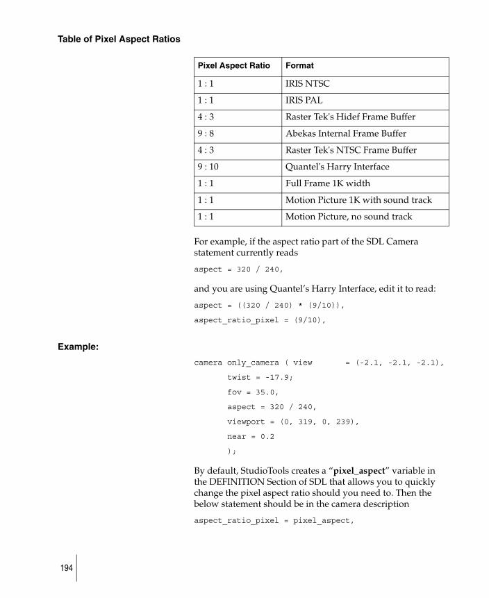
Table of Pixel Aspect Ratios
For example, if the aspect ratio part of the SDL Camera statement currently reads
aspect = 320 / 240,
and you are using Quantel’s Harry Interface, edit it to read:
aspect = ((320 / 240) * (9/10)),
aspect_ratio_pixel = (9/10),
Example:
camera only_camera ( view = (-2.1, -2.1, -2.1),
twist = -17.9;
fov = 35.0,
aspect = 320 / 240,
viewport = (0, 319, 0, 239),
near = 0.2
);
By default, StudioTools creates a “pixel_aspect” variable in the DEFINITION Section of SDL that allows you to quickly change the pixel aspect ratio should you need to. Then the below statement should be in the camera description
aspect_ratio_pixel = pixel_aspect,
Pixel Aspect Ratio Format
1 : 1 IRIS NTSC
1 : 1 IRIS PAL
4 : 3 Raster Tek's Hidef Frame Buffer
9 : 8 Abekas Internal Frame Buffer
4 : 3 Raster Tek's NTSC Frame Buffer
9 : 10 Quantel's Harry Interface
1 : 1 Full Frame 1K width
1 : 1 Motion Picture 1K with sound track
1 : 1 Motion Picture, no sound track
194
active
Syntax:
active = <scalar>
Range:
0 (FALSE) or not 0 (TRUE)
Default:
TRUE
Purpose:
A Boolean flag that controls whether the camera will be used or not.
Comments:
This component may be animated.
Example:
active = FALSE
aspect
Syntax:
aspect = <scalar>
Range:
>0
Default:
1.0
195
Purpose:
This defines the ratio of the x and y dimensions of the window of the world. All visible objects are projected onto this window. In order for objects not to be distorted, the aspect ratio of the physical rectangle on the screen defined by the viewport statement must be the same as the value for aspect. Some output devices do not have square pixels. In order to create undistorted images, the following formula provides the correct aspect ratio: ( vp width / vp height ) * ( pixel width / pixel height ) where “vp” means viewport.
Starting version 7, the definition of aspect has changed slightly. It just indicates the pixel aspect ratio. The viewport is no longer a needed consideration because it is computed on-the-fly in version 7.
Comments:
This component may be animated.
Example:
aspect = ((xright – xleft) / (yhigh – ylow))
This example uses an expression made up of system defined variables. It is appropriate for an image that will be output to a device that has square pixels.
aspect_ratio_pixel
Syntax:
aspect_ratio_pixel = <scalar>
Range:
>0
Default:
1.0
196
Purpose:
This defines the pixel aspect ratio appropriate for different output devices.
Comments:
This component may be animated.
Example:
aspect_ratio_pixel = 1.0
This example is appropriate for an image that will be output to a device that has square pixels.
auto_focus
Syntax:
auto_focus= <scalar>
Range:
0 (FALSE) or 1 (TRUE)
Default:
FALSE
Purpose:
This is relevant when depth of field is turned on. If auto_focus is turned on, then the focus point is the lookat point of the camera. If auto_focus is turned off, then the focal_distance is used to determine the focus point.
Comments:
This component may be animated.
Example:
auto_focus = FALSE
197
depth_file
Syntax:
depth_file = <filename>
Purpose:
This defines the filename used as output for a floating point depth value for each pixel, instead of a color or mask value.
For users who want to read the file, or write utilities that make use of the file, the format is as follows:
1 integer (the file's magic number) should be 55655
1 short (the image width, or X dimension)
1 short (the image height, or Y dimension)
X * Y floats (representing the pixels)
To use the results as an 8-bit texture file, see depthmap in the Standalone Utilities manual.
depth_of_field
Syntax:
depth_of_field = <scalar>
Range:
0 (FALSE) or not 0 (TRUE)
Default:
FALSE
Purpose:
This specifies that depth of field will be used when RayTracing. Most renderers in the world mimic a pin hole camera, which has an infinite depth of field. RayTracing allows
198
the use of real depth of field, simply and easily. Only the distance of focus in the scene, and the focal_length and f_stop of the lens have to be specified.
Comments:
This component may be animated. You must specify focal_distance if depth_of_field is TRUE.
Example:
depth_of_field = TRUE
far
Syntax:
far = <scalar>
Range:
Any positive floating point number greater than the value assigned to near.
Default:
1000
Purpose:
This sets the position of the far plane. Objects are not clipped to the far plane. However, calculations for Fog use the far value to compute the distance from the camera to the background. Objects in the scene that are further than the clipping plane will not render correctly.
Comments:
This component may be animated.
Example:
far = 50.0
199
filmaperture_x
Syntax:
filmaperture_x = <scalar>
Range:
Any positive floating point number greater than 0.
Default:
1
Purpose:
This sets the aperture width in the horizontal direction. Another term for aperture in camera terminology is film back.
Comments:
This component is only relevant for perspective cameras. The region outside of that defined by the filmaperture and filmoffset will be rendered in black.
Example:
filmaperture_x = 1.0
filmaperture_y
Syntax:
filmaperture_y = <scalar>
Range:
Any positive floating point number greater than 0.
Default:
1
200
Purpose:
This sets the aperture width in the vertical direction. Another term for aperture in camera terminology is film back.
Comments:
This component is only relevant for perspective cameras. The region outside of that defined by the filmaperture and filmoffset will be rendered in black.
Example:
filmaperture_y = 1.0
filmoffset_x
Syntax:
filmoffset_x = <scalar>
Range:
Any floating point number less than half of filmaperture_x.
Default:
0
Purpose:
This sets the film offset in the horizontal direction.
Comments:
This component is only relevant with perspective cameras. The region outside of that defined by the filmaperture and filmoffset will be rendered in black.
Example:
filmoffset_x = 0.0
201
filmoffset_y
Syntax:
filmoffset_y = <scalar>
Range:
Any floating point number less than half of filmaperture_y.
Default:
0
Purpose:
This sets the film offset in the horizontal direction.
Comments:
This component is only relevant with perspective cameras. The region outside of that defined by the filmaperture and filmoffset will be rendered in black.
Example:
filmoffset_y = 0.0
focal_distance
Syntax:
focal_distance = <scalar>
Range:
Non-negative.
Default:
none
202
Purpose:
The focal distance is the distance from the camera (lens) to a point in the scene upon which the lens is focused. The value specified is interpreted as being in units of feet to agree with depth of field charts in published guides.
Comments:
This must be specified if depth_of_field is true.
This component may be animated.
Example:
focal_distance = 15.0
focal_length
Syntax:
focal_length = <scalar>
Range:
Greater than 1
Default:
35
Purpose:
The focal length of the lens is a property of the lens. The value specified is interpreted as being in units of millimeters.
Comments:
This component may be animated.
Example:
focal_length = 50.0
203
fov
Syntax:
fov = <scalar>
Range:
0.2 to 179.
Default:
45
Purpose:
This statement sets the camera’s field of view in degrees. A setting of 40 approximates a 35mm lens, and 20 is a 50mm lens. Note that for very wide angles, the distortions are not those of an actual wide-angle optical lens. A value outside the above range will generate a run time error message.
Starting in version 6.0 of SDL, instead of specifying the field of view with fov, it is possible to specify it using aov, which stands for angle of view (this is the more classical camera terminology). Both are identical in definition. Furthermore, if the SDL file states that it is a version 6.0 file (or greater), the fov will be interpreted as cropping in the vertical direction, rather than the previously cropped horizontal direction.
Comments:
This component may be animated.
Example:
fov = 20
f_stop
Syntax:
f_stop = <scalar>
204
Range:
Non-negative.
Default:
8
Purpose:
Any good photography reference guide will contain a depth of field table giving focal distances based on focal length and f stop. You may then choose whichever focal_length / f stop combination produces the desired result, and render the image. The same reference manual will also have a section for calculating f stop and focal length directly from the focal_distance, fov and aspect ratio.
Comments:
This component may be animated.
Example:
f_stop = 5.6
mask
Syntax:
mask = <filename>
Default:
Special — see the comments.
Purpose:
To define the output destination of the mask file produced by this camera.
205
Comments:
Each camera in the MODEL section (whether instanced or literal) is capable of producing output independent of any other cameras. The output may be an image file, a mask file or both. If this (mask) component is specified, then a mask output is produced. If it is omitted, then no mask is created for this camera. A similar situation exists for the pix component. If both the pix and the mask components are absent, then either a default is used or an error occurs, depending upon the circumstances described below.
If more than one camera (either literal or instance) is present in the MODEL section, then the second one encountered and all subsequent ones must have a pix component or a mask component (or both) specified to define where the result of the rendering is to be output. If such a required component is absent, then an error condition exists and the processing is stopped with an error message. The first camera encountered must likewise have a destination for its output. However, unlike subsequent ones, the first camera has a default (an image is produced and goes to “stdout”, no mask is produced). It may also be set by the DEFINITION parameters or by the command line options. Note that if the first camera’s output is specified in more than one of the 3 possible ways (command line, operation parameter, camera component), then the command line specification will be used, if given, and failing that, the camera component will be used. Specification of camera output by use of DEFINITION parameters will only be used if no other specification has been given.
Only the first camera may have its output specified by default, or by the command line or by an DEFINITION parameter. All other cameras must have either the pix component or the mask component (or possibly, but not necessarily, both) specified.
The actual name of an output file produced by a camera (either PIX or MASK or both) may be different from what is specified by the user. The name used is comprised of four parts:
● specified
● stereo
● animation
206

● field
The first, or specified part, is exactly what was specified by the user (which may or may not have an extension. Refer to the section on filenames for more information).
The second, or stereo part, is only used when rendering stereo images. When stereo = TRUE either “_left” or “_right” will be appended to the name appropriately.
The third, or animation part, is used only when rendering an animation (that is, when animation = TRUE). A further “dot” extension is appended to the name. (This is not to be confused with a user specified extension.)
This will be a non-negative integer prefixed by a single period (“dot”). Its value will be equal to startextension for the first frame and will increment by the value of byextension for each subsequent frame produced. Refer to the descriptions on startextension and byextension in the Definition section of this manual for more information.
The fourth, or fields portion is only produced when rendering on fields (that is, when fields = TRUE). The single character “e” is appended to the names of all files produced for an “EVEN” field, and the single character “o” is appended for “ODD” ones.
Comments:
This component may be animated.
Example:
mask = ("~/mask/thisone")
matte_depth
Syntax:
matte_depth= <scalar>
Range:
-infinity to infinity
207
Default:
Purpose:
Specifies a distance in units from the eye point. Thus, positive values indicate that the matte plane is behind the camera — we recommend this be used only when you are raytracing reflections that are behind the camera. Note that the matte_plane description must precede the matte_depth and matte_order descriptions.
Note: Specify either matte_depth or matte_order, not both.
Example:
matte_depth = -10.0
matte_order
Syntax:
matte_order= <scalar>
Range:
-infinity to infinity
Default:
Purpose:
Specifies a distance in units from the eye point. A positive value indicate that the matte_plane is behind the entire geometry database, and a negative value indicate that the matte-plane is in front of the database. Larger values determine the front-ordering of these matte-planes. Note that the matte_plane description must precede the matte_depth and matte_order descriptions.
208
A matte_order value of 0 indicates NO ordering. This means that it resides exactly at the back of any rendering (sort of like a backdrop).
Specify either matte_depth or matte_order, not both.
Example:
matte_order = -0.500000
matte_plane
Syntax:
matte_plane= <texture>
Range:
Default:
Purpose:
Specifies the name of a file texture to be used as a matte plane.
At the moment, only file textures (like “file” and “stencil”) are being handled in matte-planes in the interactive package. In the Scene Description Language, other texture-types can be applied to matte-planes.
Example:
texture back (
procedure = Stencil,
mask_level = 1.0,
mask_blur = 0.0,
edge_blend = 0.0,
positive_key = OFF,
image_file = "/usr/u/myname/user_data/demo/pix/back.pix.1",
209
key_masking = ON,
color_key = (1.000000, 1.000000, 1.000000),
hue_range = 0.500000,
sat_range = 0.500000,
val_range = 0.500000,
threshold = 0.500000,
active = TRUE,
rgbmult = (1.000000, 1.000000, 1.000000),
rgboffset = (0.000000, 0.000000, 0.000000),
ucoverage = 1.000000,
vcoverage = 1.000000,
utranslate = 0.000000,
vtranslate = 0.000000,
uwrap = TRUE,
vwrap = FALSE,
urepeat = 320.000000 / 321.000000,
vrepeat = 241.000000 / 241.000000,
uoffset = 50.000000 / 321.000000,
voffset = 0.000000 / 241.000000
);
This is an example of using a matte-plane with the filename "back.pix.1" and chroma-keying specified. If no chroma-keying or matte-files are specified, then the "file" texture is used instead.
motion_blur
Syntax:
motion_blur = <scalar>
Default:
ON
210
Range:
0 (OFF) or non-zero (ON)
Purpose:
If motion_blur is turned on for the file, this flag indicates that motion blur should be calculated for this object.
Example:
motion_blur = ON
near
Syntax:
near = <scalar>
Range:
Unexpected results may be produced when near is assigned a very small value. Therefore, the recommended minimum setting is 0.1. The number must be greater than 0.
Default:
0.2
Purpose:
This sets the position of the near clipping plane. It truncates the pyramid of vision when objects come too close to the apex. Interior sectional views of objects are attained by setting the near plane within the objects.
Comments:
This component may be animated.
Example:
near = 1.0
211
perspective
Syntax:
perspectivet = <scalar>
Range:
0 (FALSE) or not 0 (TRUE)
Default:
TRUE
Purpose:
A Boolean flag that controls the projection scheme. The camera uses perspective projection if the flag is TRUE; otherwise, it uses orthographic projection.
Comments:
If perspective = FALSE, win_xsize and win_ysize must be specified.
Example:
perspective = FALSE
pix
Syntax:
pix = <filename>
Default:
Special — see the comments.
Purpose:
Defines the destination of the image file produced by the camera.
212
Comments:
Each camera in the MODEL section (whether instanced or literal) is capable of producing output independent of any other camera. The output may be an image file, a mask file or both. If this (pix) component is specified, then an image output is produced. If it is omitted, then no image is created for this camera. A similar situation exists for the mask component. If both the pix and the mask components are absent, then either a default is used or an error occurs, depending upon the circumstances given below.
If more than one camera (either literal or instance) is present in the MODEL Section, then the second one encountered and all subsequent ones must have a pix component or a mask component (or both) specified to define where the result of the rendering is to be output. If such a required component is absent, then an error condition exists and the processing is stopped with an error message. The first camera encountered must likewise have a destination for its output.
However, unlike subsequent ones, the first camera has a default (an image is produced and goes to “stdout”, no mask is produced). It may also be set by the DEFINITION Section parameters or by the command line options. Note that if the first camera’s output is specified in more than one of the 3 possible ways (command line, operation parameter, camera component), then the command line specification will be used, if given, and failing that, the camera component will be used. Specification of camera output by use of DEFINITION parameters will only be used if no other specification has been given.
Only the first camera may have its output specified by default, or by the command line or by an DEFINITION parameter. All other cameras must have either the pix component or the mask component (or possibly, but not necessarily, both) specified.
The actual name of an output file produced by a camera (either PIX or MASK or both) may be different from what is specified by the user. The name used is comprised of four parts:
● specified
● stereo
213
● animation
● field
The first, or specified part, is exactly what was specified by the user (which may or may not have an extension. Refer to the section on filenames for more information).
The second, or stereo part, is only used when rendering stereo images. When stereo = TRUE either “_left” or “_right” will be appended to the name appropriately.
The third, or animation part, is used only when rendering an animation (that is, when animation = TRUE). A further “dot” extension is appended to the name. (This is not to be confused with a user-specified extension.)
This will be a non-negative integer prefixed by a single period (“dot”). Its value will be equal to STARTEXTENSION for the first frame and will increment by the value of BYEXTENSION for each subsequent frame produced. Refer to the descriptions on startextension and byextension in the Definition section of this manual for more information.
The fourth, or fields portion is only produced when rendering on fields (that is, fields = TRUE). The single character “e” is appended to the names of all files produced for an “EVEN” field, and the single character “o” is appended for “ODD” ones.
Comments:
This component may be animated.
Example:
pix = ("~/pix/thatone")
placement_fit_code
Syntax:
placement_fit_code = <scalar>
214
Range:
0, 2
Default:
0.0
Purpose:
Placement_fit_code is only relevant when the aspect ratio of the filmback does not match the aspect ratio of the rendering resolution. If there is a mismatch in aspect ratios, then there will be some clipped out regions in the resultant rendering. There are three variations in clipping out regions:
● 0: best fit in both vertical and horizontal direction.
● 1: fit in the horizontal direction, and clipped in the vertical direction.
● 2: fit in the vertical direction, and clipped in the horizontal direction.
Example:
placement_fit_code = 0.0
placement_shift
Syntax:
placement_shift = <scalar>
Range:
-1, 1
Default:
0.0
215
Purpose:
Placement_shift is only relevant when the aspect ratio of the film back does not match the aspect ratio of the rendering resolution. If there is a mismatch in aspect ratios, there will be some clipped out regions in the resultant rendering, as described above. When placement_shift is set to 0, the image will be centered so that the clipped out regions will be equally divided on both ends. If set to -1, then the image is shifted to the right (or to the top), where one end of the clipped out region becomes totally visible. A setting of 1 has a similar effect, but in the opposite direction.
Example:
placement_shift = 0.0
scaling_factor
Syntax:
scaling_factor= <scalar>
Range:
> 0
Default:
1.0
Purpose:
Scaling_factor is only relevant to depth_of_field. This provides for a better control of the fuzzy effects from depth of field. The larger the scaling_factor, the more amplified the depth of field’s fuzzy effects.
Example:
scaling_factor = 1.0
216
twist
Syntax:
twist = <scalar>
Range:
unlimited
Default:
0.0
Purpose:
The twist sets the degrees of tilt away from the camera’s vertical axis. Tilting the camera clockwise with a positive twist setting makes the world look like it is tilted to the left.
Comments:
This component may be animated. twist is ignored if up is specified.
Example:
twist = (animate( roll, frame ))
units_to_feet
Syntax:
units_to_feet = <scalar>
Range:
greater than 0.0
Default:
0.0
217
Purpose:
units_to_feet allows the definition of focal_distance in units other than feet (for example, in meters). The value of units_to_feet is the length of the unit as expressed in terms of feet. In case of focal distance defined in meters, units_to_feet will be 0.3048 since 0.3048 meters equals one foot.
Comments:
This component may be animated.
Example:
units_to_feet = 1.0
up
Syntax:
up = <triple>
Range:
unlimited
Default:
0.0, 1.0, 0.0
Purpose:
The up vector is used as a reference to define the angle of twist, and is one of the components affecting the orientation of the camera.
Comments:
This component may be animated. twist is ignored if up is specified.
Example:
up = (animate( roll, frame ))
218
view
Syntax:
view = <triple>
Range:
There are no limits to value; however, if 0.0 or very large numbers are used (for example, 10000000), unpredictable behavior may occur.
Default:
Not applicable — see below.
Purpose:
This describes the location in space, in absolute world coordinates, toward which the camera is directed. The three components of the triple correspond to the x, y and z coordinates, respectively. To always look at the same point, use this statement. If not specified, the camera simply looks down the axis of the viewing pyramid ( 0, 0, -1 relative to the camera) and is controlled by transforming the camera as a whole.
Comments:
This component may be animated.
Example:
view = some_trip_var_name
viewport
Syntax:
viewport = ( <scalar> , <scalar> , <scalar> , <scalar> )
219
Range:
unbounded
Default:
(0, 644, 0, 485)
Purpose:
This statement maps, in pixels, the window of the world onto the screen. The first two numbers set the beginning and the end of the horizontal coordinates. The second two numbers set the beginning and the end of the vertical coordinates. Note that this is the mapping of the viewing frustrum, and it does not affect the area to be rendered as defined in the DEFINITION Section. The origin of the screen is the lower left hand corner.
Comments:
Starting version 7, the viewport information will be ignored. A viewport is automatically computed based on the information of the film back, film offset, etc. If a viewport was used for partial image rendering, this is now easily specifiable in the interactive package without having to tweak with numbers.
Example:
viewport = (0, 319, 0, 239)
win_xsize
Syntax:
win_xsizet = <scalar>
Range:
unbounded
220
Default:
Not applicable - see below.
Purpose:
win_xsize defines the horizontal window size for orthographic rendering. The unit of measure is the unit of measure used for the grid in the StudioTools system; by default, centimeters.
Comments:
This component works only when perspective = FALSE.
Example:
win_xsize = 18.948872
win_ysize
Syntax:
win_ysizet = <scalar>
Range:
unbounded
Default:
Not applicable - see below.
Purpose:
win_ysize defines the vertical window size for orthographic rendering. The unit of measure is the unit of measure used for the grid in the StudioTools system; by default, centimeters.
Comments:
This component works only when perspective = FALSE.
221

Example:
win_ysize = 13.462891
222

Curve Data Type
Declaration:
curve <name> ( <component list> );
Reference:
<name>
Literal:
curve ( <component list> )
Purpose:
A curve is a non-uniform rational b-spline. It may be instanced as an object in the MODEL Section. A curve may be specified as a literal or as a variable. If specified as a variable, it must have a name. The following components must be specified between the parentheses:
● cvs
● degree
● knots
All components are specified using a keyword=value form, and are separated by commas. The components may be specified in any order.
Example:
curve curve#2 (
degree = 3,
knots = ( 0.0 , 0.0 , 0.0 , 1.0 , 1.0 ,
1.0 ),
cvs = (
cv( ( -0.50656, -0.43168, 0.0 ), 1.0 ),
cv( ( -0.50998, -0.5717 , 0.0 ), 1.0 ),
223
cv( ( -0.44153, -0.62975, 0.0 ), 1.0 ),
cv( ( -0.29094, -0.62975, 0.0 ), 1.0 ) )
);
cvs
Syntax:
cvs = ( ( <cv>, <cv>, … <cv> ),
( <cv>, <cv>, … <cv> ),
.
.
.
( <cv>, <cv>, … <cv> ) )
Range:
Any collection of valid cvs (i.e., see the CV Data Type).
Default:
None. Must be specified.
Purpose:
This defines the control vertices for the curve.
Example:
cvs = (
cv( ( -0.50656, -0.43168, 0.0 ), 1.0 ),
cv( ( -0.50998, -0.5717 , 0.0 ), 1.0 ),
cv( ( -0.44153, -0.62975, 0.0 ), 1.0 ),
224
cv( ( -0.29094, -0.62975, 0.0 ), 1.0 ) )
);
degree
Syntax:
degree = <scalar>
Range:
1 to 33
Default:
none
Purpose:
To describe the degree of the NURBS curve. To define a syntactically correct curve, there must be at least degree + 1 control vertices.
Comments:
As the degree of the surface increases, it is a good idea to increase the rendering subdivisions for the object defined with that curve.
Example:
degree = 3
knots
Syntax:
knots = ( <scalar>, <scalar>, …<scalar> )
225
Range:
Each entry must evaluate to a real number, which must be greater than or equal to the value of its predecessor.
Default:
None. Must be specified.
Purpose:
This defines the knot vector in the curve’s direction. It must match with number of CVs given.
Comments:
It may be animated.
Example:
knots = ( 0, 1, 2, 3, 4, 5 )
226
CV Data Type
Declaration:
cv <name> ( <triple>, <scalar> ) ;
Reference:
<name>
Literal:
cv ( <triple>, <scalar> )
Purpose:
This defines a cv. A cv may be specified as a literal or as a variable. If specified as a variable, it must have a name. All of its components are identified by position rather than by keywords. They are interpreted as
( (x, y, z), w )
x, y, and z, are the coordinates of the cv; w is its weight.
Example:
cv u0 ((-1, 0, 0), 1);
cv u1 (( 0, 0, 0), 1);
cv u3 (( 1, 0, 0), 1);
cv u3 (( 2, 0, 0), 1);
227
Face Data Type
Declaration:
face <name> ( <component list> ) ;
Reference:
<name>
Literal:
face ( <component list> )
Purpose:
A face is an object that may be instanced in the MODEL section. It defines a planar surface whose boundary is given by a spline curve.
Comments:
A face may be specified as a literal or as a variable. If specified as a variable, it must have a name. Any of the following components may be specified between the parentheses:
● active
● boundaries
● casts_shadow
● clusters
● cvs
● degree
● divisions
● knots
● light_list
● motion_blur
● motion_blur_shading_samples
● motion_blur_texture_sample_level
228
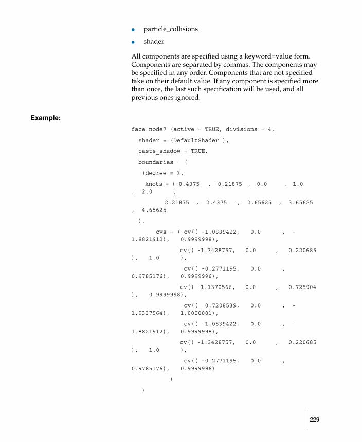
● particle_collisions
● shader
All components are specified using a keyword=value form. Components are separated by commas. The components may be specified in any order. Components that are not specified take on their default value. If any component is specified more than once, the last such specification will be used, and all previous ones ignored.
Example:
face node7 (active = TRUE, divisions = 4,
shader = (DefaultShader ),
casts_shadow = TRUE,
boundaries = (
(degree = 3,
knots = (-0.4375 , -0.21875 , 0.0 , 1.0 , 2.0 ,
2.21875 , 2.4375 , 2.65625 , 3.65625 , 4.65625
),
cvs = ( cv(( -1.0839422, 0.0 , -1.8821912), 0.9999998),
cv(( -1.3428757, 0.0 , 0.220685 ), 1.0 ),
cv(( -0.2771195, 0.0 , 0.9785176), 0.9999996),
cv(( 1.1370566, 0.0 , 0.725904 ), 0.9999998),
cv(( 0.7208539, 0.0 , -1.9337564), 1.0000001),
cv(( -1.0839422, 0.0 , -1.8821912), 0.9999998),
cv(( -1.3428757, 0.0 , 0.220685 ), 1.0 ),
cv(( -0.2771195, 0.0 , 0.9785176), 0.9999996)
)
)
229
));
active
Syntax:
active = <scalar>
Range:
0 (FALSE) or not 0 (TRUE)
Default:
TRUE
Purpose:
A Boolean flag that controls whether the face is visible or not.
Comments:
This component may be animated. This is provided so the user can cause an object to suddenly appear or disappear in an animation.
Example:
active = TRUE
boundaries
Syntax:
boundaries = (degree = <scalar>, knots = (....), ( <boundary description> ),
( <boundary description> ),
.
.
230
.
( <boundary description> ) )
Default:
none.
Purpose:
This defines the shape of the face, including the outer face and all inner faces.
Comments:
The definition consists of a list of curves. The first curve in the list is considered the outer face—all subsequent curves are considered inner faces. Each curve specified has its own set of 3 components: cvs, to define the curve according to its polynomial basis; knots, to define the polynomial basis; and divisions, to define the quality of the rendering approximation. These components are discussed separately below. The boundaries component must be specified, and it must contain at least one curve. There may be any number of additional curves. Each curve in the list (even if there is only one) must be enclosed within parentheses, and the list itself must also be enclosed within parentheses. The boundaries component may not be animated.
Example:
boundaries = (
(degree = 3,
knots = (-0.4375 , -0.21875 , 0.0 , 1.0 , 2.0 ,
2.21875 , 2.4375 , 2.65625 , 3.65625 , 4.65625
),
cvs = ( cv(( -4.4072771, 0.0 , -7.6529346), 0.9999998),
cv(( -5.4600935, 0.0 , 0.897299 ), 1.0 ),
231
cv(( -1.1267598, 0.0 , 3.9786241), 0.9999996),
cv(( 4.623239 , 0.0 , 2.9515047), 0.9999998),
cv(( 2.9309711, 0.0 , -7.8625975), 1.0000001),
cv(( -4.4072771, 0.0 , -7.6529346), 0.9999998),
cv(( -5.4600935, 0.0 , 0.897299 ), 1.0 ),
cv(( -1.1267598, 0.0 , 3.9786241), 0.9999996)
)
)
casts_shadow
Syntax:
casts_shadow = <scalar>
Range:
0 (FALSE) or not 0 (TRUE)
Default:
TRUE
Purpose:
A Boolean flag that controls whether or not this face will cast a shadow.
Comments:
This component may be animated. Note that a transparent or semitransparent object will not cast a shadow when RayCasting.
232
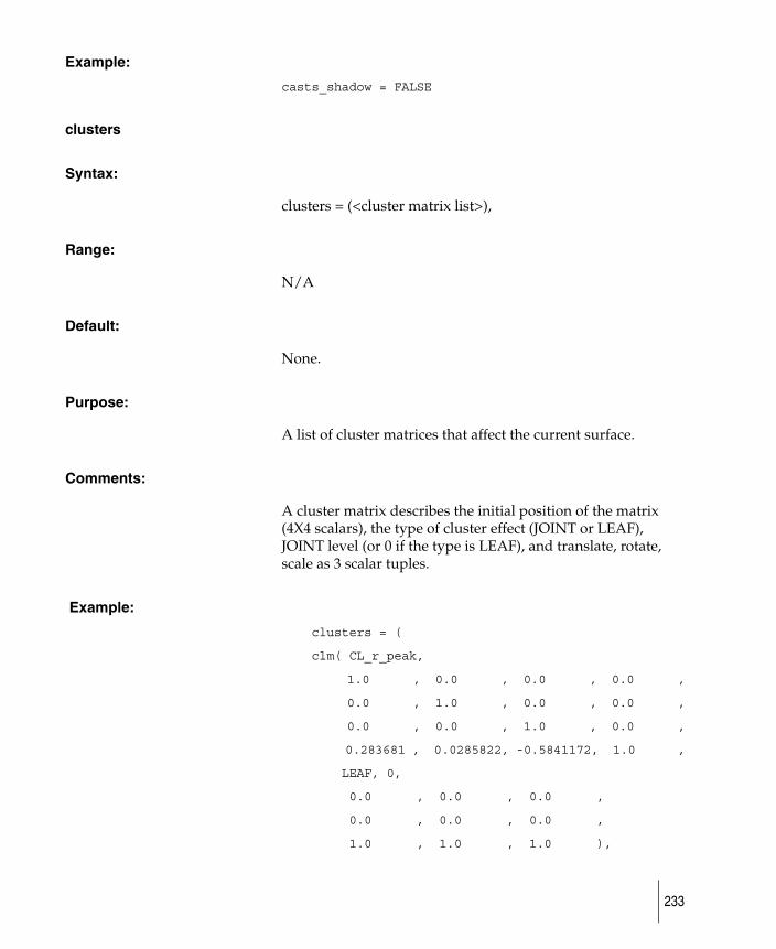
Example:
casts_shadow = FALSE
clusters
Syntax:
clusters = (<cluster matrix list>),
Range:
N/A
Default:
None.
Purpose:
A list of cluster matrices that affect the current surface.
Comments:
A cluster matrix describes the initial position of the matrix (4X4 scalars), the type of cluster effect (JOINT or LEAF), JOINT level (or 0 if the type is LEAF), and translate, rotate, scale as 3 scalar tuples.
Example:
clusters = (
clm( CL_r_peak,
1.0 , 0.0 , 0.0 , 0.0 ,
0.0 , 1.0 , 0.0 , 0.0 ,
0.0 , 0.0 , 1.0 , 0.0 ,
0.283681 , 0.0285822, -0.5841172, 1.0 ,
LEAF, 0,
0.0 , 0.0 , 0.0 ,
0.0 , 0.0 , 0.0 ,
1.0 , 1.0 , 1.0 ),
233

clm( CL_knot45_section0_Rwrist,
1.0 , 0.0 , 0.0 , 0.0 ,
0.0 , 1.0 , 0.0 , 0.0 ,
0.0 , 0.0 , 1.0 , 0.0 ,
0.283681 , 0.0285822, -0.5841172, 1.0 ,
LEAF, 0,
0.0 , 0.0 , 0.0 ,
0.0 , 0.0 , 0.0 ,
1.0 , 1.0 , 1.0 )
clm( CL_cluster#10,
1.0 , 0.0 , 0.0 , 0.0 ,
0.0 , 1.0 , 0.0 , 0.0 ,
0.0 , 0.0 , 1.0 , 0.0 ,
0.283681 , 0.0285822, -0.5841172, 1.0 ,
JOINT, 3,
-0.2398842, -0.0303474, 0.0 ,
0.0 , 0.0 , 0.0 ,
1.0 , 1.0 , 1.0 ) ),
cvs
Syntax:
cvs = ( <cv>, <cv>, … <cv> )
Default:
None. Must be specified.
Purpose:
Defines the control vertices for a face boundary curve.
Comments:
It may be animated.
234
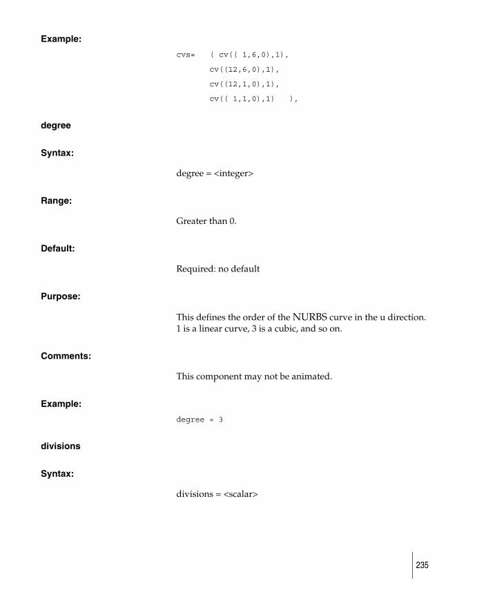
Example:
cvs= ( cv(( 1,6,0),1),
cv((12,6,0),1),
cv((12,1,0),1),
cv(( 1,1,0),1) ),
degree
Syntax:
degree = <integer>
Range:
Greater than 0.
Default:
Required: no default
Purpose:
This defines the order of the NURBS curve in the u direction. 1 is a linear curve, 3 is a cubic, and so on.
Comments:
This component may not be animated.
Example:
degree = 3
divisions
Syntax:
divisions = <scalar>
235
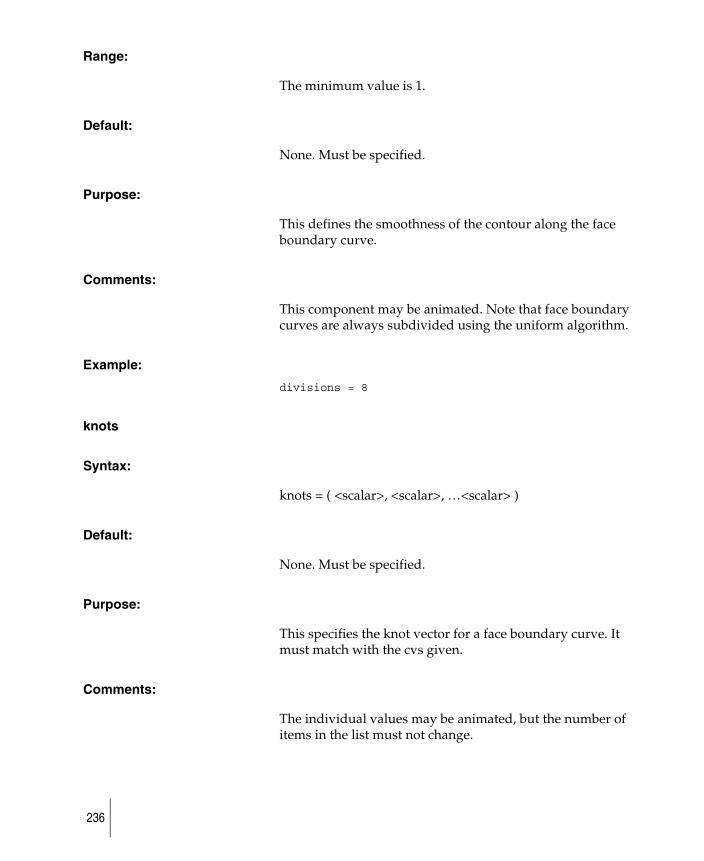
Range:
The minimum value is 1.
Default:
None. Must be specified.
Purpose:
This defines the smoothness of the contour along the face boundary curve.
Comments:
This component may be animated. Note that face boundary curves are always subdivided using the uniform algorithm.
Example:
divisions = 8
knots
Syntax:
knots = ( <scalar>, <scalar>, …<scalar> )
Default:
None. Must be specified.
Purpose:
This specifies the knot vector for a face boundary curve. It must match with the cvs given.
Comments:
The individual values may be animated, but the number of items in the list must not change.
236
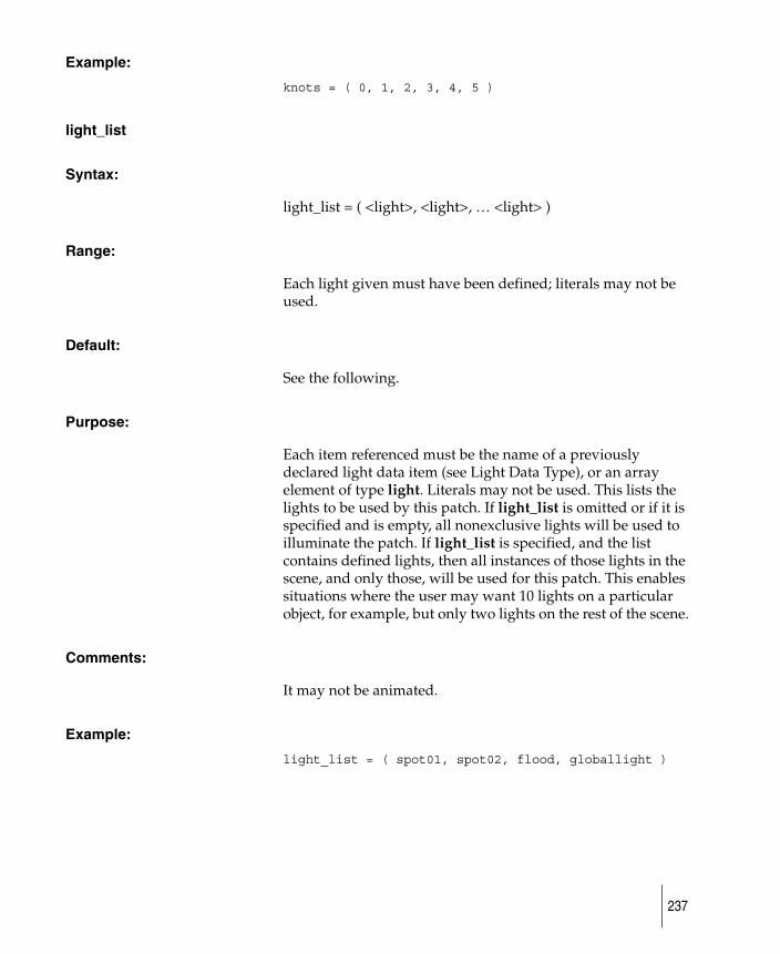
Example:
knots = ( 0, 1, 2, 3, 4, 5 )
light_list
Syntax:
light_list = ( <light>, <light>, … <light> )
Range:
Each light given must have been defined; literals may not be used.
Default:
See the following.
Purpose:
Each item referenced must be the name of a previously declared light data item (see Light Data Type), or an array element of type light. Literals may not be used. This lists the lights to be used by this patch. If light_list is omitted or if it is specified and is empty, all nonexclusive lights will be used to illuminate the patch. If light_list is specified, and the list contains defined lights, then all instances of those lights in the scene, and only those, will be used for this patch. This enables situations where the user may want 10 lights on a particular object, for example, but only two lights on the rest of the scene.
Comments:
It may not be animated.
Example:
light_list = ( spot01, spot02, flood, globallight )
237
motion_blur
Syntax:
motion_blur = <scalar>
Default:
ON
Range:
0 (OFF) or non-zero (ON)
Purpose:
If motion_blur is turned on for the file, this flag indicates that motion blur should be calculated for this object.
Example:
motion_blur = ON
motion_blur_shading_samples
Syntax:
motion_blur_shading_samples = <scalar>
Default:
3 - for bump or displacement mapped objects
1 - for all other objects
Range:
>= 3 for bump or displacement mapped objects
> 0 for all other objects
238
Purpose:
If motion_blur is turned on for the file, this flag indicates the number of samples done for shading of motion-blurred objects.
Example:
motion_blur_shading_samples = 1
motion_blur_texture_sample_level
Syntax:
motion_blur_texture_sample_level = <scalar>
Default:
3
Range:
0-5
Purpose:
If motion_blur is turned on for the file, this flag indicates the level of sampling done for texturing of motion-blurred objects. A 0 indicates no extra samples (lowest quality) and 5 means highest quality motion-blurred textures. Note, this flag does not apply to bump or displacement mapping.
Example:
motion_blur_texture_samples = 3
particle_collisions
Syntax:
particle_collisions = BOUNDING_BOX_COLLISIONS | OFF | GEOMETRY_COLLISIONS
239
Range:
As above
Default:
OFF
Purpose:
To define which objects collide with particles.
Example:
particle_collisions = BOUNDING_BOX_COLLISIONS
shader
Syntax:
shader =( <shader>)
or
shading = ( <shader>, <shader>, …
<shader> )
Range:
The shaders given may be variables or array elements of type shader (see Shader Data Type). Note that there is no such thing as a literal shader.
Default:
None. Must be specified.
Purpose:
This specifies which shading characteristics are assigned to the face.
240
Comments:
This component may be animated. If a list of shaders is specified, they will be visible in the order given.
Example:
shader = ( label_1, bottle_1 )
241
Filename Data Type
Declaration:
filename <name> (“quoted string” <scalar> );
or
filename <name> (“quoted string”);
Reference:
<name>
Literal:
(“quoted string” <scalar> )
or
(“quoted string”)
Purpose:
This defines a filename. A filename may be specified as a literal or as a variable. If specified as a variable, it must have a name. A filename has at least one, and optionally two components. These are identified by position rather than by keyword. The first component is a UNIX path. If only the first component is present, then the path must specify a file. The second component is an extension. If it is specified, then its value is converted to an integer and appended (using the normal “dot” extension form) to the path. If an extension component is supplied, then it will always be used. This does NOT depend upon any sense of Animation.
The total filename (path plus extension) must identify a file.
A filename may specify a full or relative UNIX path. Relative paths are applied with respect to the current working directory when the renderer is invoked.
A filename variable may receive either form (single component or two component) in an assignment.
242
Example:
filename anim_texture_in(“~/texture/hoops” (frame -1));
Note that the expression (frame -1) is not necessarily integer in value. That is, it could be 3.5 if rendering on fields. The extension will be converted to an integer, however. Thus, the field where frame equals 4.0 and the field were frame equals 4.5 will both generate “~/texture/hoops.4” in this example.
243
Light Data Type
Declaration:
light <name> (procedure=<procedure name>, <component list> ) ;
Reference:
<name> ( )
Literal:
light (<component list>)
Purpose:
This defines a source of illumination.
Comments:
A light is an object that may be instanced in the MODEL Section. Light is used to illuminate a scene when the rendering mode is raytrace or raycast. Lights are ignored when the rendering mode is wireframe. Only lights of type spotlight can cast a shadow in the RayCaster, but any type of light may cast a shadow in the RayTracer. A light may be specified as a literal or a variable. If specified as a variable, it must have a name. Any of the following components may be given between the parentheses. Please note that particle system components are described following the light data type section.
● active
● ambient_shade
● arc
● bias
● color
● concentric
● cone_end_radius
244

● decay
● decay_start
● depth_input
● depth_output
● direction
● directional
● directionality
● directional_turbulence
● dropoff
● dropoff_start
● flare_color
● flare_color_spread
● flare_focus
● flare_horizontal
● flare_intensity
● flare_length
● flare_num_circles
● flare_max_size
● flare_min_size
● flare_vertical
● fog_intensity
● fog_opacity
● fog_radial_noise
● fog_samples
● fog_spread
● fog_star_level
● fog_type
● fog_2D_noise
● force_type
● force_intensity
● glow_intensity
245
● glow_opacity
● glow_radial_noise
● glow_rotation
● glow_spread
● glow_star_level
● glow_type
● glow_2D_noise
● halo_intensity
● halo_spread
● halo_type
● hexagon_flare
● intensity
● LENS_FLARE
● model
● noise_threshold
● noise_uoffset
● noise_uscale
● noise_voffset
● noise_vscale
● penumbra
● psys_blob_lighting
● psys_blob_map
● psys_blob_noise
● psys_blob_noise_frequency
● psys_blob_threshold
● psys_blur_quality
● psys_branch_angle
● psys_buoyancy
● psys_collisions
● psys_color
● psys_curl
246
● psys_density
● psys_elasticity
● psys_emission
● psys_end_frame
● psys_filename
● psys_friction
● psys_glow_intensity
● psys_hair_length_max
● psys_hair_length_min
● psys_hair_stiffness
● psys_hair_segments
● psys_hit_method
● psys_incandescence
● psys_lifespan_min
● psys_lifespan_max
● psys_mass
● psys_motion_type
● psys_num_children
● psys_parent_shading
● psys_particles_per_sec
● psys_randomization
● psys_render_type
● psys_size
● psys_speed
● psys_speed_decay
● psys_speed_range
● psys_split_time
● psys_start_frame
● psys_surface_shading
● psys_time_random
● psys_translucence
247
● psys_transparency
● psys_use_particle_file
● radial
● radial_noise_frequency
● shadow
● shadow_dither
● shadowmult
● shadowoffset
● shadow_blend_offset
● shadow_edge_quality
● shadow_min_depth
● shadow_output
● shadow_resolution
● shadow_samples
● shape
● shine_along
● size
● soft_shadows
● specular
● split_velocity_min
● spread
● star_points
● torus_radius
● turbulence_animated
● turbulence_granularity
● turbulence_intensity
● turbulence_persistence
● turbulence_roughness
● turbulence_space_resolution
● turbulence_spread
● turbulence_time_resolution
248
● turbulence_variability
● up
● use_old_shadow_map_algorithm
● use_shadow_map
All components are specified using a keyword=value form. The components may appear in any order. When more than one component is used, they must be separated by commas. Not all components are optional. Components which are not specified take on their default value. If any component is specified more than once, the last such specification will be used, and all previous ones will be ignored. Not all components are meaningful in all combinations. In situations where a component is not meaningful, any specification of it will be ignored with no ill effect.
Example:
light sun(model=directional, direction=(1,1,1));
active
Syntax:
active = <scalar>
Range:
0 (FALSE) or not 0 (TRUE).
Default:
TRUE
Purpose:
A switch which turns the light off if it is FALSE and on if it is TRUE.
249
Comments:
This component may be animated. active is appropriate for all lighting models.
Example:
active = fmod(frame,2)
ambient_shade
Syntax:
ambient_shade = <scalar>
Range:
0.0 to 1.0. Values outside this range are replaced by 0 or 1 as appropriate, and a warning is issued.
Default:
0.5
Purpose:
Defines the omnidirectionality of an ambient light.
Comments:
This component may be animated. If ambient_shade is set to 0.0, the total illumination will come from all directions and objects will show no edge definition. Set to 1.0, the illumination will come solely from the light position and objects will show definite edge contrast. ambient_shade is only appropriate for the ambient lighting model.
Example:
ambient_shade = 1.0
250
arc
Syntax:
arc = <scalar>
Range:
0.0 to 360.0
Default:
360
Purpose:
This value defines the portion of the swept volume. A value of 360 degrees represents the entire volume.
Comments:
This value is only applicable to the CONE, SPHERE, TORUS and CYLINDER volume lights.
Example:
arc = 360.0
bias
Syntax:
bias = ( <scalar> , <scalar> )
Range:
Non-negative.
Default:
( 0.3, 0.4 )
251
Purpose:
This parameter is now obsolete
Used for RayCasting only. The two <scalar>s are interpreted as the minimum and maximum values, respectively. Together they define the range for which each surface point is randomly moved towards the eye before it is determined whether or not it is in shadow. The minimum must be smaller than the maximum. Either or both of the <scalar>s may be animated.
Comments:
The bias component is required to prevent incorrect self shadowing on an object when a z value of a point on the surface is compared to the depth map z from a nearby, but different point on the same surface. If the depth map z is smaller, the point on the surface will appear to be in shadow when it isn’t. The stochiastic bias allows the user to correct this while still allowing a surface to curve over and legitimately shadow itself without aliasing. This, unfortunately, has the effect of moving the shadow boundary away from its true position. bias values must therefore be large enough to eliminate self-shadowing artifacts, yet small enough to avoid any noticeable problems from the offset boundary positions.
From a practical point of view, the minimum and maximum bias are measured in world space and therefore depend on the size of the scene. For a 100 x 100 x 100 scene, a typical bias would be 0.3 to 0.4. If the shadow looks ragged in places, increase the minimum and/or maximum. If the shadow boundary has moved noticeably and looks incorrect, decrease the minimum and/or maximum. For a 10 x 10 x 10 scene, a bias of 0.04 to 0.07 works well.
bias is appropriate for the spotlight lighting model. It is ignored for point, infinite and ambient lights. It is ignored even for spotlights if shadow has not been set to TRUE. Note that depth maps are only used for RayCasting.
Example:
bias = (0.4, 0.7)
252
color
Syntax:
color = <triple>
Range:
-infinity to infinity
Default:
( 255.0, 255.0, 255.0 )
Purpose:
This defines the color of the light.
Comments:
This component may be animated. A color component is appropriate for all lighting models. Note that if you use a negative number, the light will suck illumination away from the scene.
Example:
color = ( 0, 0, 255 )
concentric
Syntax:
concentric = <scalar>
Range:
-1.0 to 1.0
Default:
1.0
253

Purpose:
This value defines how much the in-out direction contributes to the light direction.
This value defines the intensity of light radial to the light's central axis. For a spherical volume light, a value of 1 imitates a point light with all illumination moving out from the center. A value of -1 reverses that effect so that illumination comes from the outside of the sphere towards the central axis. With a value of 0, directional and radial values must be used to give illumination direction along the major axis or radially around the major axis.
Example:
concentric = 0.25
cone_end_radius
Syntax:
cone_end_radius = <scalar>
Range:
-infinity to infinity
Default:
0.1
Purpose:
This value defines the radius of the end of the cone. A value of 0 makes the volume light a true cone, whereas a value of 1 effectively reduces the shape of the light to a cylinder. This value may be negative, which will have the effect of reversing the direction of the cone.
Comments:
This value is only applicable to the CONE volume light.
254
Example:
cone_end_radius = 1.0
decay
Syntax:
decay = <scalar>
Range:
0, 1, 2, or 3. The value given is treated as an integer.
Default:
0
Purpose:
This is used to determine how intensity decreases with distance.
Comments:
This component may be animated. Set decay to 0 for constant intensity (the light shines forever). Set decay to 1 for a decrease that is proportional to the distance from the light. Set decay to 2 for a decrease that is proportional to the square of the distance.Set decay to 3 for a decrease that is proportional to the cube of the distance. decay is appropriate for point and spot lighting models. It is ignored for directional and ambient lights.
For volume lights,
No decay light reaches everything within the volume, nothing outside.
>0 Light intensity decreases from the center towards the edges of the volume.
255
.
Example:
decay = 2
decay_start
Syntax:
decay_start = <scalar>
Range:
0.0 to 1.0
Default:
0.0
Purpose:
This value defines how far out from the centre of the volume the decay starts.
Example:
decay_start = 0.0
0.5 linear dropoff from the middle to the edges. With a value close to 1, intensity drops off very fast from the middle With a value close to 0, intensity drops off slowly in the middle and fast near the edges.
<0 Light intensity decreases from the edges towards the middle
Shape Decay
BOX and SPHERE all directions from the center
CYLINDER and CONE
in the direction of the principal axis
TORUS perpendicular to the principal axis
256
depth_input
Syntax:
depth_input = <filename>
Range:
none
Default:
none
Purpose:
This is only relevant for a shadow-casting spot light. If there is a depth_input file, then instead of generating the shadow map (expensive), it reads this file instead to get the depth values. This is useful only for non-moving objects and lights within the scene.
Example:
depth_input = “depth_input_file”
depth_output
Syntax:
depth_output = <filename>
Range:
none
Default:
none
257
Purpose:
This is only relevant for a shadow casting spot light. If there is a depth_output file, then the shadow map generated is written to this file. This is useful if the depth_input is also the same filename, which means the renderer will generate the depth map just once, and write it to this file, then reuse it for subsequent frames.
Example:
depth_output = “depth_output_file”
direction
Syntax:
direction = <triple>
Range:
unbounded, but cannot be (0,0,0).
Default:
( 0.0, 0.0, 1.0 )
Purpose:
This simulates placing the source of illumination at infinity.
Comments:
The triple provides a direction vector pointing towards the light. The magnitude of the vector is immaterial. This component may be animated using a motion path, or by otherwise varying the value of the triple. direction is appropriate for the directional lighting model. It is ignored for point, spot, ambient, area and linear lights
Example:
direction=(1,1,1)
258
directional
Syntax:
directional = <scalar>
Range:
-1.0 - 1.0
Default:
0.0
Purpose:
This value defines how much the primary axis direction contributes to the light direction
Comments:
For volume lights only.
Example:
directional = 1.0
directionality
Syntax:
directionality = <scalar>
Range:
0.0 - 1.0
Default:
1.0
259
Purpose:
This value defines how much the direction of the light is taken into account in the lighting calculation. A value of 0 acts like an ambient light; a value of 1 acts like a directional light.
Comments:
For volume lights only.
Example:
directionality = 1.0
directional_turbulence
Syntax:
directional_turbulence = <boolean>
Range:
ON/OFF
Default:
ON
Purpose:
Used to define a wind field.
Comments:
Turbulence is mostly used when the volume light is used to define a wind field, but it also defines the light direction, and can be used to get flickering sorts of light effects. The turbulence is defined as if it were inside a “box”, and the box is placed appropriately when you need to evaluate the turbulence at a point.
Example:
directional_turbulence = ON
260
dropoff
Syntax:
dropoff = <scalar>
Range:
If a negative number is provided, 0 is used; no error message is given. Although any positive real number can be used, the dropoff will be severe beyond the range of 5-7; numbers greater than 20 have little effect unless intensity is quite high.
Default:
0
Purpose:
dropoff describes the rate at which illumination will fall off from the center of a spot light to the edge of the cone of illumination (determined by the angle set in spread). A value of 0 means there is no dropoff — the edge is as bright as the center.
For volume lights, this value controls the rate at which light intensity decreases from the center to the edge of the light. It only applies to CONE and CYLINDER types of volume lights, and the dropoff is away from the principal axis of the light. The range is from 0 to infinity. The range usually used is from 0 to 50. Values of 1.0 and less give practically identical results, that is no discernible intensity decrease along the radius of the beam. The default value is 0.0, which means there is no dropoff. This is very similar to the way that spotlights work.
Comments:
This component may be animated. dropoff is appropriate for the spot lighting model. It is ignored for point, directional and ambient lights.
Example:
dropoff = 0.5
261
dropoff_start
Syntax:
dropoff_start = <scalar>
Range:
0.0 to 1.0
Default:
0.5
Purpose:
This value defines how far out from the centre axis of the volume the drop-off starts.
Example:
dropoff_start = 0.5
flare_color
Syntax:
flare_color = <triplet>
Range:
-infinity to infinity
Default:
(160, 160, 255)
Purpose:
If textured then each circle in the flare will contain the texture, scaled to exactly fit inside the circle. Circular ramp textures can be used to create colorful rainbow flare effects.
262
Example:
flare_color = (160, 160, 255),
flare_color_spread
Syntax:
flare_color_spread = <scalar>
Range:
0 to 1
Default:
0.5
Purpose:
This is the amount that the hue of individual circles is randomized about the flare color. Note that the flare_color must be at least partially saturated (that is, not white or grey) to see this effect.
Example:
flare_color_spread = 0.5,
flare_focus
Syntax:
flare_focus = <scalar>
Range:
0 to 1
Default:
0.6
263
Purpose:
This controls the sharpness of circle edges. At a value of 1, the edges are totally sharp, at zero the circles are very blurry.
Example:
flare_focus = 0.6,
flare_horizontal
Syntax:
flare_horizontal = <scalar>
Range:
-infinity to infinity
Default:
0
Purpose:
This parameter, with flare_vertical, controls the axis of the flare effect relative to the center of the image. As the light source moves, the flare will appear to rotate through this point.
Example:
flare_horizontal = 0,
flare_intensity
Syntax:
flare_intensity = <scalar>
Range:
0 to infinity
264
Default:
1
Purpose:
This is the scale for the brightness of the flare effect.
Example:
flare_intensity = 1,
flare_length
Syntax:
flare_length = <scalar>
Range:
0 to infinity
Default:
1
Purpose:
This controls how long the flare effect is relative to the light location. If the value is small, then all the circles in the flare will bunch up on the light. If it is large then the circles will get spread out off the edge of the image.
Example:
flare_length = 1,
flare_num_circles
Syntax:
flare_num_circles = <scalar>
265
Range:
0 to infinity
Default:
20
Purpose:
This is the number of spots created along the length of the flare effect.
Comment:
Very large numbers of spots can be expensive to render, especially if the size is large and the flare color is textured.
Example:
flare_num_circles = 20,
flare_max_size
Syntax:
flare_max_size = <scalar>
Range:
-infinity to infinity
Default:
1
Purpose
The size of the circles is randomized between these two values.
266
Example:
flare_max_size = 1,
flare_min_size
Syntax:
flare_min_size = <scalar>
Range:
-infinity to infinity
Default:
0.1
Purpose:
The size of the circles is randomized between flare_min_size and flare_max_size.
Example:
flare_min_size = 0.1,
flare_vertical
Syntax:
flare_vertical = <scalar>
Range:
-infinity to infinity
Default:
0
267

Purpose:
This parameter, with flare_horizontal, controls the axis of the flare effect relative to the center of the image. As the light source moves, the flare will appear to rotate through this point.
Example:
flare_vertical = 0,
fog_intensity
Syntax:
fog_intensity
Range:
-infinity to infinity
Default:
1.0
Purpose:
Set the brightness of the fog illumination.
Comments:
The fog illumination simulates a 3D volume of scattered light. Point lights simulate a spherical volume of fog. If the fog_intensity is too high, then the glow will look like a glowing orb. Use glow and/or halo effects in conjunction with fog glow when a bright, focused center to the glow is desired.
Example:
fog_intensity = 0.5
268
fog_opacity
Syntax:
fog_opacity = <scalar>
Range:
-infinity to infinity
Default:
0.0
Purpose:
To allow an illuminated fog to obscure objects.
Comments:
Normally the fog glow is added on top of the light in the scene. If the opacity is greater than zero, then the fog will be more opaque where it is brightest. This is useful when simulating fire and smoke effects, which frequently do not let all the light in a scene pass through. Black smoke can be created by making the light color near black and the opacity high (around 10.0).
Example:
fog_opacity = 5.0
fog_radial_noise
Syntax:
fog_radial_noise = <scalar>
Range:
-infinity to infinity
269
Default:
0.0
Purpose:
To simulate explosion and starburst effects.
Comments:
Similar to glow_radial_noise.
This effect is currently two-dimensional.
Example:
fog_radial_noise = 0.5
fog_samples
Syntax:
fog_samples= <scalar>
Range:
Any value greater than 0 up to the resolution of the shadow depth map.
Default:
50
Purpose:
This parameter is only relevant when light fog shadows are to be computed. The higher the value for this parameter, the better the fog shadow quality. Usually, the default is good enough, but sometimes where there is little detail, such a value can miss important fog shadow features, or produce noisy results. By increasing this value (up to the depth map
270
resolution), the quality will be increased, but so will the performance.
Example:
fog_samples = 50;
fog_spread
Syntax:
fog_spread = <scalar>
Range:
-infinity to infinity
Default:
1.0
Purpose:
fog_spread has different effects on point lights and spot lights. On point lights, it determines the size of the glowing spherical volume of fog. On spotlights, it determines how concentrated or focused the beam is (higher fog_spread creates more uniform spotlight beams, while at lower values, the center of the beam will appear brighter).
Comments:
Use the decay parameter on spot lights to modify the way the beam falls off with distance from the lightsource.
Example:
fog_spread = .2
271
fog_star_level
Syntax:
fog_star_level = <scalar>
Range:
-infinity to infinity
Default:
0.0
Purpose:
To create radial explosion effects and control fog glow direction.
Comments:
See glow_star_level.
Example:
fog_star_level = 1.0
fog_type
Syntax:
fog_type = OFF | LINEAR_GLOW | EXPONENTIAL_GLOW | BALL_GLOW
Range:
0 (OFF) to 3 (BALL_GLOW)
Default:
OFF
272
Purpose:
The fog_type specifies the way that the intensity of fog illumination falls off from the center of the light.
Comments:
All different types currently produce a LINEAR_GLOW; however, BALL_GLOW will provide sharper thresholds at the edge when fog_opacity is not 0.0. In spot lights, the decay will determine how fast the light falls off from the center of the light.
Shadows can be cast into volumes of fog by using spot lights with shadow = ON and fog_type = LINEAR_GLOW (Raycaster Only).
Currently fog glow is only available for point lights and spot lights.
Example:
fog_type = LINEAR_GLOW
fog_2D_noise
Syntax:
fog_2D_noise = <scalar>
Range:
-infinity to infinity
Default:
0.0
Purpose:
Simulate smoke and fire effects using two-dimensional noise.
273
Comments:
The noise is generated on a plane that is centered at the location of the light and always oriented towards the line of sight. To create the illusion of illuminated smoke around a glowing light source, set fog_2D_noise to about 0.5 and animate slowly the noise_uoffset and noise_voffset values. The smoke will appear to slowly drift by the light.
If a spotlight is rotated, the beam will appear to move through smoke in a room. If you want the noise to remain locked on to the beam as it moves (for example, for a rocket thruster), the glow_rotation will need to be animated to match the spotlight orientation.
Example:
fog_2D_noise = .5
force_type
Syntax:
force_type = OFF | GRAVITY | MAGNET | WIND | DRAG
Range:
As above
Default:
OFF
Purpose:
To define force emission from a light.
Example:
force_type = GRAVITY
274
force_intensity
Syntax:
force_intensity = <scalar>
Range:
-infinity to infinity
Default:
1.0
Purpose:
To set the intensity of the force.
Example:
force_intensity = 1.0
glow_intensity
Syntax:
glow_intensity = <scalar>
Range:
-infinity to infinity
Default:
1.0
Purpose:
Set the brightness of the light glow.
275
Comments:
If the light has a non-zero decay, then the brightness of the glow will vary with the distance of the light. As the glow of the light becomes intense, the size of the glow will appear to increase, especially when the center of the glow washes out. This simulates what would naturally happen with a real light and film. Negative glows will tend to subtract from other glows, thus a light with a negative BALL_GLOW could be put along with a light with a standard glow, resulting in a hole in the center of the glow.
Example:
glow_intensity = 3.0
glow_opacity
Syntax:
glow_opacity = <scalar>
Range:
-infinity to infinity
Default:
0.0
Purpose:
To allow a light glow to obscure objects.
Comments:
Normally the light glow is added on top of the light in the scene. If the opacity is greater than zero, then the glow will be more opaque where it is brightest. This is useful when simulating fire and smoke effects, which frequently do not let all the light in a scene pass through. However, it is generally better to use a fog glow for these effects. Also, if you want the glow to appear on the background only, and not obscure any objects, then an opacity value of -1 will do this.
276
Example:
glow_opacity = 5.0
glow_radial_noise
Syntax:
glow_radial_noise = <scalar>
Range:
-infinity to infinity
Default:
0.0
Purpose:
To simulate starburst effects and eyelashes refracting light.
Comments:
Negative values will create a thicker noise. Use the radial_noise_frequency to adjust the smoothness of this effect.
Example:
glow_radial_noise = 0.5
glow_rotation
Syntax:
glow_rotation = <scalar> (in degrees)
Range:
-infinity to infinity
277
Default:
0.0
Purpose:
To rotate the various glow and fog noise and star effects about the location of the light.
Comments:
Affects glow_2D_noise, fog_2D_noise, glow_star_level, fog_star_level, glow_radial_noise and fog_radial_noise.
Example:
glow_rotation = 45.0
glow_spread
Syntax:
glow_spread = <scalar>
Range:
-infinity to infinity
Default:
1.0
Purpose:
glow_spread determines the general size of the glow effect.
Comments:
glow_spread also affects the size of the SPECTRAL and RAINBOW effects. Negative values can have odd but useful effects. For example if the glow_spread = -6.0 and the glow_2D_noise = 1.0, an image of a fiery bubble is created.
278
Example:
glow_spread = 0.1
glow_star_level
Syntax:
glow_star_level = <scalar>
Range:
-infinity to infinity
Default:
0.0
Purpose:
To simulate camera star filter effects.
Comments:
This is often effective when combined with a high frequency glow_radial_noise. Use star_points to set the number of points on the star. If the star_points = 1.0, comet like effects are possible. The star can be rotated by using glow_rotation.
Example:
glow_star_level = 4.0
glow_type
Syntax:
glow_type = OFF | LINEAR_GLOW | EXPONENTIAL_GLOW | BALL_GLOW | SPECTRAL | RAINBOW | LENS_FLARE
279
Range:
0 (OFF) to 6 (LENS_FLARE)
Default:
OFF
Purpose:
The glow_type specifies the way that the intensity and color of a light glow falls off from the center of the light.
Comments:
All the parameters associated with light glow work with all of the glow types. For instance a RAINBOW glow may be combined with glow_star_level of 1.0 and star_points of 4 to create a colored refraction grating effect.
Example:
glow_type = EXPONENTIAL
OFF NO glow.
LINEAR_GLOW glow slowly diminishes from center of light
EXPONENTIAL_GLOW glow quickly diminishes from center of light
BALL_GLOW glow diminishes faster towards a distance from glow center specified by the glow_spread.
SPECTRAL lower wavelengths (red) refract (or spread) more than the higher frequencies (blue).
RAINBOW simulates refraction due to water droplets in air. The radius of the rainbow is determined by the glow_spread parameter.
LENS_FLARE concentric circles of color.
280

glow_2D_noise
Syntax:
glow_2D_noise = <scalar>
Range:
-infinity to infinity
Default:
0.0
Purpose:
Simulate smoke and fire effects using a two-dimensional noise.
Comments:
The noise is generated on a plane that is centered at the location of the light and always oriented towards the line of sight. To create the illusion of illuminated smoke around a glowing light source, set glow_2D_noise to about 0.5 and animate slowly the noise_uoffset and noise_voffset values. The smoke will appear to slowly drift by the light.
Generally fog glow (fog_2D_noise) is better for creating smoke and fire effects, because these are 3D effects. (glow_2D_noise cannot be occluded by objects, for example.)
Example:
glow_2D_noise = .5
halo_intensity
Syntax:
halo_intensity
281
Range:
-infinity to infinity
Default:
1.0
Purpose:
Set the brightness of the light halo..
Comments:
If the light has a non-zero decay, the brightness of the halo will vary with the distance of the light. As the halo of the light becomes intense, the size of the halo will appear to increase, especially when the center of the halo washes out.
Example:
halo_intensity = 3.0
halo_spread
Syntax:
halo_spread = <scalar>
Range:
-infinity to infinity
Default:
1.0
Purpose:
halo_spread determines the general size of the glow effect.
282
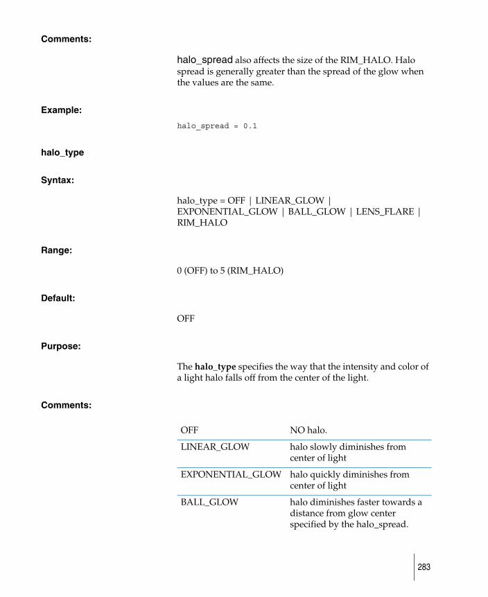
Comments:
halo_spread also affects the size of the RIM_HALO. Halo spread is generally greater than the spread of the glow when the values are the same.
Example:
halo_spread = 0.1
halo_type
Syntax:
halo_type = OFF | LINEAR_GLOW | EXPONENTIAL_GLOW | BALL_GLOW | LENS_FLARE | RIM_HALO
Range:
0 (OFF) to 5 (RIM_HALO)
Default:
OFF
Purpose:
The halo_type specifies the way that the intensity and color of a light halo falls off from the center of the light.
Comments:
OFF NO halo.
LINEAR_GLOW halo slowly diminishes from center of light
EXPONENTIAL_GLOW halo quickly diminishes from center of light
BALL_GLOW halo diminishes faster towards a distance from glow center specified by the halo_spread.
283
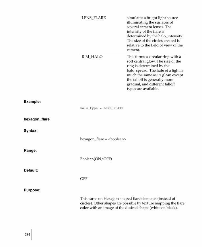
Example:
halo_type = LENS_FLARE
hexagon_flare
Syntax:
hexagon_flare = <boolean>
Range:
Boolean(ON/OFF)
Default:
OFF
Purpose:
This turns on Hexagon shaped flare elements (instead of circles). Other shapes are possible by texture mapping the flare color with an image of the desired shape (white on black).
LENS_FLARE simulates a bright light source illuminating the surfaces of several camera lenses. The intensity of the flare is determined by the halo_intensity. The size of the circles created is relative to the field of view of the camera.
RIM_HALO This forms a circular ring with a soft central glow. The size of the ring is determined by the halo_spread. The halo of a light is much the same as its glow, except the falloff is generally more gradual, and different falloff types are available.
284
Example:
hexagon_flare = OFF,
intensity
Syntax:
intensity = <scalar>
Range:
-infinity to infinity
Default:
1.0
Purpose:
This sets the brightness of the light.
Comments:
This component may be animated. The value is checked at usage time, and if negative, stops execution. Set intensity to 0.0 for no illumination, 1.0 for normal illumination; 5.0 would be a very bright illumination. If you set intensity to a negative number, it will suck light away from the scene.
Example:
intensity = 2
LENS_FLARE
Syntax:
LENS_FLARE = <boolean>
Range:
Boolean (OFF/ON)
285
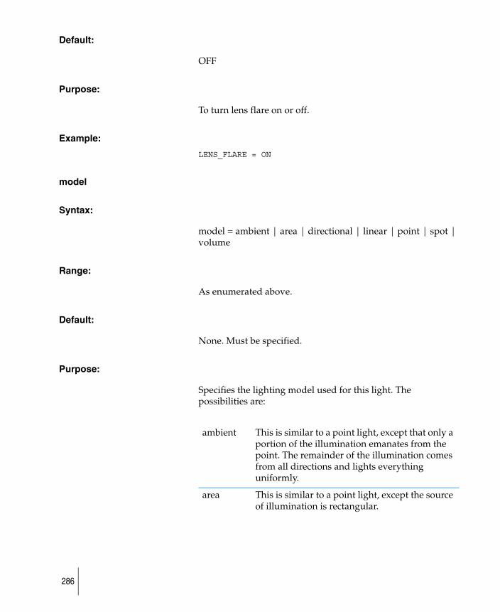
Default:
OFF
Purpose:
To turn lens flare on or off.
Example:
LENS_FLARE = ON
model
Syntax:
model = ambient | area | directional | linear | point | spot | volume
Range:
As enumerated above.
Default:
None. Must be specified.
Purpose:
Specifies the lighting model used for this light. The possibilities are:
ambient This is similar to a point light, except that only a portion of the illumination emanates from the point. The remainder of the illumination comes from all directions and lights everything uniformly.
area This is similar to a point light, except the source of illumination is rectangular.
286

Comments:
The lighting model is not animatable. The value is checked to be one of the above at definition time. Improper specification terminates execution with an error message.
directional In this case, the source of illumination is infinitely far away from the scene. The actual position of the light data item in the scene description is immaterial. Its orientation, however, is used. Rotations will affect the direction of the light.
linear This is similar to a point light, except the source of illumination is a line of light placed in the scene.
point This is the case where light emanates from a point somewhere in the scene. That point is the same as the position of the light object in the scene description. (That is, the origin of the light is (0,0,0) relative to the light object, and is transformed using current_transformation.) Note that the light emanates in all directions.
spot This is similar to a point light in that it is a point source, and it exists somewhere in the scene. It is different, however, in that it radiates illumination in a cone about a specific direction. The position of the source in the scene is the same as the position of the light object in the scene description. (That is, the origin of the light is (0,0,0) relative to the light object, and is transformed using current_transformation.)
volume defines a closed volume in which objects will be illuminated, and nothing outside the volume is directly illuminated by the light. Within the volume, the direction and intensity can vary in many different parameters. A volume light is a convenient way to “link” a light spatially, instead of by object. The main use of the volume light is to be a force field generator and particle emitter.
287
Example:
model = directional
noise_threshold
Syntax:
noise_threshold = <scalar>
Range:
0 to 1.0
Default:
1.0
Purpose:
This is a cutoff value for 2D noise. As the threshold is lowered to zero, fog_2D_noise and glow_2D_noise break up into smaller and smaller particles.
Comments:
This is useful for simulating globular clusters, ejecta from explosions, snow and rain effects, especially when the noise u and v scale is high. It can also help make flames and smoke more patchy.
Example:
noise_threshold = 0.8
noise_uoffset
Syntax:
noise_uoffset = <scalar>
288
Range:
-infinity to infinity
Default:
0.0
Purpose:
To offset the horizontal position of 2D noise.
Comments:
Can create the look of smoke moving past a light when animated. Rain and snow effects are also possible.
The noise will wrap after an offset of 1.0, which is useful in creating animated loops.
Example:
noise_uoffset = .5
noise_uscale
Syntax:
noise_uscale = <scalar>
Range:
0 to infinity
Default:
1.0
Purpose:
To change the scale of glow_2D_noise and fog_2D_noise in the horizontal.
289

Comments:
This is useful for creating effects like layered fog and tall flames. Also, if the noise_uscale and noise_vscale are animated from high to low values, the noise will appear to fly apart like an explosion.
Example:
noise_uscale = 3.0
noise_voffset
Syntax:
noise_voffset = <scalar>
Range:
-infinity to infinity
Default:
0.0
Purpose:
To offset the vertical position of the 2D noise.
Comments:
Can create the look of smoke moving past a light when animated. Rain and snow effects are also possible.
the noise will wrap after an offset of 1.0, which is useful in creating animated loops.
Example:
noise_voffset = .5
290
noise_vscale
Syntax:
noise_vscale = <scalar>
Range:
0 to infinity
Default:
1.0
Purpose:
To change the scale of the glow and fog 2D_noise in the vertical.
Comments:
This is useful for creating effects like layered fog and tall flames. Also, if the noise_uscale and noise_vscale are animated from high to low values, the noise will appear to fly apart like an explosion.
Example:
noise_vscale = 3.0
penumbra
Syntax:
penumbra = <scalar>
Range:
absolute: -90, 90 (degrees)
useful range: -20, 20
291
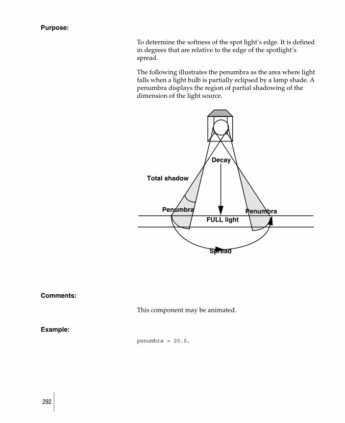
Purpose:
To determine the softness of the spot light’s edge. It is defined in degrees that are relative to the edge of the spotlight’s spread.
The following illustrates the penumbra as the area where light falls when a light bulb is partially eclipsed by a lamp shade. A penumbra displays the region of partial shadowing of the dimension of the light source.
Comments:
This component may be animated.
Example:
penumbra = 20.0,
FULL light
Penumbra
Total shadow
Decay
Penumbra
Spread
292
radial
Syntax:
radial = <scalar>
Range:
-1.0 - 1.0
Default:
0.0
Purpose:
This value defines how much the spin direction contributes to the field value.
Comments:
For volume lights only.
Example:
radial = 0.0
radial_noise_frequency
Syntax:
radial_noise_frequency = <scalar>
Range:
-infinity to infinity
Default:
0.5
293
Purpose:
To control the smoothness of the glow and fog radial noises.
Comments:
See glow_radial_noise.
Example:
radial_noise_frequency = 3.0
shadow
Syntax:
shadow = <scalar>
Range:
0 (FALSE) or not 0 (TRUE)
Default:
FALSE
Purpose:
A boolean indicating whether this light will cast shadows or not. If shadow is TRUE, the light will cast shadows.
Comments:
This component may be animated. For RayCasting, shadow is appropriate for the spot lighting model and ignored for point, directional and ambient lights. For RayTracing, shadow is appropriate for all lighting models.
Example:
shadow = TRUE
294
shadow_dither
Syntax:
shadow_dither = <scalar>
Range:
0.0 to 1.0
Default:
1.0
Purpose:
Values less than 1.0 allow a tradeoff between soft jittered shadow edges and less noisy but more defined shadow edges.
Comments:
Used with soft shadowing in the raytracer. If this value is zero, then the soft shadows will break apart into multiple shadows, determined by the shadow_samples parameter. If shadow_samples = 4, then the light will appear to cast 4 separate shadows. The separation of the shadows is determined by the light radius and the distance of the light away. As the shadow_dither parameter is increased to 1.0, the four shadows would then each spread until they merged into one soft shadow.
for animations it is best to leave this parameter at 1.0, because the shadows may move a little as the view changes.
SEE soft_shadows.
Raytracer ONLY.
Example:
shadow_dither = 0.5
295
shadowmult
Syntax:
shadowmult = <scalar>
Range:
Not negative; effective range is 0.0 to 4.0
Default:
1
Purpose:
This parameter is obsolete effective this software release. Similar to blurmult for textures, shadowmult is a scaling factor for the size of the sample region for the depth map. The default size of the sample region is 4 x 4 pixels in the depth map.
Values lower than 0.5 (without using shadowoffset) are prone to aliasing and banding. The actual formula used to calculate the size of the sample area is:
numpixels = (4 * shadowmult) + shadowoffset
Care should be taken that numpixels does not become negative or 0. shadowmult is appropriate for the spotlight lighting model. It is ignored for point, infinite and ambient lights. It is ignored even for spotlights if shadow has not been set to TRUE. Note that depth maps are only used for RayCasting. shadowmult is meaningless and ignored when RayTracing.
Comments:
This component may be animated.
Example:
shadowmult = 3.0
296
shadowoffset
Syntax:
shadowoffset = <scalar>
Range:
unbounded; effective range is -2 to 8.
Default:
0
Purpose:
This parameter is obsolete effective this release. Similar to bluroffset for textures, shadowoffset modifies the sampling region of the depth map. shadowoffset adds a specified amount to the pixel area of the sampling region. The default sampling region is 4 by 4 pixels in the depth map. The actual formula used to calculate the sample region is:
numpixels = (4 * shadowmult) + shadowoffset
It is always square, numpixels to a side. Care should be taken that numpixels does not become negative or 0. shadowoffset is appropriate for the spotlight lighting model. It is ignored for point, infinite and ambient lights. It is ignored even for spotlights if shadow has not been set to TRUE. Note that depth maps are only used for RayCasting. shadowoffset is meaningless and ignored when RayTracing.
Comments:
This component may be animated.
Example:
shadowoffset = 0.5
297
shadow_blend_offset
Syntax:
shadow_blend_offset = <scalar>
Range:
0 to infinity
Default:
1.0
Purpose:
This is useful for removal of self shadowing.
Comments:
shadow_blend_offset offsets the depth of the blended shadow samples, but not the depth of the center sample. At zero, the sample region is a plane tangent to the light direction vector. As the value increases, the sample region becomes a cone with the outer edges towards the light. Its use is somewhat similar to the old bias_max; however, it cleans up self-shadows without sacrificing the tightness of a shadow relative to a very close object.
Raycast Shadows ONLY
Example:
shadow_blend_offset = .3
shadow_edge_quality
Syntax:
shadow_edge_quality = <scalar>
298
Range:
1 to infinity
Default:
2
Purpose:
Sets the blur filter size for shadow depth maps.
Comments:
At low values (1 or 2) slight staircasing can appear around shadow edges. Increasing the shadow_edge_quality will correct this problem, but increase rendering time a bit. Also the edge will become softer, requiring larger shadow_resolution values if hard edges are desired.
shadow_resolution should be used to control general level of blur, not shadow_edge_quality.
Raycast Shadows ONLY
Example:
shadow_edge_quality = 3
shadow_min_depth
Syntax:
shadow_min_depth = <scalar>
Range:
0.0 to infinity
Default:
0.05
299
Purpose:
To correct self shadowing problems in raycast shadows. The shadow_min_depth is the world space distance that a point is moved towards a spotlight before shadowing is calculated.
Comments:
If this value is 0, than an object will shadow itself by 50% (if it casts shadows) when the light is at an inclined angle to the surface. A relatively small shadow_min_depth value can bring the surface out of its own shadow, especially when combined with the shadow_blend_offset parameter. Also, if the surface does not need to cast shadows, only to receive them, turn shadow casting off on the object (then a shadow_min_depth of 0 is fine). The most typical example of this is a groundplane.
If shadow_min_depth is too high, shadows will not be cast from very close objects.
This parameter is similar to the old bias_min parameter, but much smaller correction values are now possible.
Raycast Shadows ONLY
Example:
shadow_min_depth = 0.03
shadow_output
Syntax:
shadow_output = <filename>
Range:
none
Default:
none
300
Purpose:
Specifies the file in which to store an 8-bit version of the depth map. This is useful if you want to create a bump map from the geometry, but is not required otherwise. shadow_output is appropriate for the spot lighting model. It is ignored for point, infinite and ambient lights. It is ignored even for spotlights if shadow has not been set to TRUE. Note that depth maps are only used for RayCasting. shadow_output is meaningless and ignored when RayTracing. For details on the differences between RayCasting with shadows and RayTracing, please refer to the User’s Guide.
Comments:
This component may be animated using the normal filename mechanisms.
Example:
shadow_output = “texture/new.bump” /* no frame extension */
or
shadow_output = (“texture/new.bump”frame) /* with frame extension */
shadow_resolution
Syntax:
shadow_resolution = <scalar>
Range:
any value between 8 and 8192
Default:
512
301
Purpose:
Defines the size of shadow depth maps used in raycasting. Large shadow_resolution values provide sharper edged shadows but at a cost in memory and rendering time.
Comments:
Very soft and smooth shadows are possible with a shadow_resolution setting around 50. Low resolutions have the added advantage of being fast to render and taking up little memory.
The shadow_resolution is the primary factor determining the softness of shadows, but the spotlight spread and shadow_edge_quality also affect the general level of blur. The shadow map is defined relative to the cone of the spotlight; so a tightly focused spread will create sharper shadows. A spread of 90 will require a shadow_resolution 2 times that of a spread of 45 in order to match.
Raycast Shadows ONLY
Example:
shadow_resolution = 55
shadow_samples
Syntax:
shadow_samples = <scalar>
Range:
1 to infinity
Default:
2
302
Purpose:
Set the minimum number of shadow feeler rays per sample (used to create raytracer soft shadows).
Comments:
A large value will result in slower rendering times, but smoother quality soft shadows.
SEE soft_shadows
Raytracer ONLY.
Example:
shadow_samples = 8
shape
Syntax:
shape = BOX_VOLUME | SPHERE_VOLUME | CYLINDER_VOLUME | CONE_VOLUME | TORUS_VOLUME
Range:
One of the above.
Default:
SPHERE_VOLUME
Purpose:
This defines the shape of the volume light in space. The choices are:
● BOX
● SPHERE
● CYLINDER
● CONE
303
● TORUS
The shapes of the volume light can be further modified by applying transformations to the dag node(s) above the volume light.
Comments:
Volume lights only.
Example:
shape = SPHERE_VOLUME
shine_along
Syntax:
shine_along = <triple>
Range:
Any set of coordinates in world space (but must be different than the light itself).
Default:
( 0.0, 0.0, 0.0 )
Purpose:
The triple gives the x, y and z coordinates describing the location of the center of illumination by the spotlight.
Comments:
This component may be animated using a motion path or by otherwise varying the value of the triple. shine_along is appropriate for the spot lighting model. It is ignored for point, directional and ambient lights.
Example:
shine_along = (20,5,-1)
304
size
Syntax:
size = <scalar>
Range:
Between 256 and 8192.
Default:
512
Purpose:
This parameter is obsolete effective this software release. size defines the resolution of depth maps used to cast shadows when RayCasting. Increasing the size will provide more detailed shadows, and will also increase the rendering time and the amount of memory used. A size of 512 uses 1 Mbyte of memory, a size of 1024 uses 4 Mbytes of memory.
Comments:
This component may be animated. size is appropriate for the spot lighting model. It is ignored for point, directional and ambient lights. It is ignored even for spotlights if shadow has not been set to TRUE. Note that depth maps are only used for RayCasting. The size component is meaningless and ignored when RayTracing.
Example:
size = 256
soft_shadows
Syntax:
soft_shadows = <scalar>
305
Range:
0 (FALSE) or not 0 (TRUE)
Default:
FALSE
Purpose:
If TRUE, then soft shadowing is enabled in StudioTools RayTracing.
Comments:
The nature of soft shadows created is determined by the distance of the light from the object casting shadows, combined with the light_radius parameter. Shadows are generated to match a globe-shaped light with the specified radius (in world space units). If the light source is small and/or far away, then hard-edged shadows will result. Shadows become softer-edged as the light’s radius increases, as happens in the real world. However, because of super-sampling, the region of partial shadow (penumbra) can become noisy. To correct this, turn up the number of samples used, adjusting either the shadow_samples level (on the light) or the global aalevelmin and aalevelmax. Note that if fast_shading is turned on, the number of shadow samples per pixel will equal the shadow_samples level, and will not be affected by the aalevel. Also, due to a blending function used, soft_shadows can be useful even when the light_radius = 0 and the shadow_samples = 1. This method helps avoid jaggies on shadow boundaries when fast_shading is used.
soft_shadows works for StudioTools RayTracing only.
Example:
soft_shadows = TRUE
306
specular
Syntax:
specular = <boolean>
Range:
ON/OFF
Default:
ON
Purpose:
If set to ON, then the light will contribute to the specular component. It is useful to turn this OFF when using a negative volume light to remove light.
Comments:
Volume lights only.
Example:
specular = ON
split_velocity_min
Syntax:
split_velocity_min = <scalar>
Range:
0 to infinity
Default:
5
307
Purpose:
Appears only if psys_collisions are set to ON. This provides a limit on the speed a particle must be moving when it collides with an object to determine if the particle splits.
Example:
split_velocity_min = 5
spread
Syntax:
spread = <scalar>
Range:
2 to 179. The absolute value is used. This value is clipped to 179 if the magnitude is too large. Similarly, if the magnitude is less than 0.2, it is set to 0.2 to avoid numeric instabilities.
Default:
40.0 (degrees)
Purpose:
spread provides the angle of illumination from a spotlight in degrees.
Comments:
This component may be animated. The smaller the value, the tighter the spotlight will appear to be. If a negative value is specified, the sign is ignored. spread is appropriate for the spot lighting model. It is ignored for point, directional and ambient lights.
Example:
spread = 15
308
star_points
Syntax:
star_points = <scalar>
Range:
0 to infinity
Default:
4.0
Purpose:
To set the number of points on star filters. (see glow_star_level.)
Comments:
Values of 1 and 2 are frequency useful. For example if star_points = 1.0 and glow_star_level = 1.0 and the glow_type = RAINBOW, then a familiar rainbow arch will be generated.
Example:
star_points = 5.0
torus_radius
Syntax:
torus_radius = <scalar>
Range:
-infinity to infinity
Default:
0.0
309
Purpose:
This is the ratio of the minor radius to the major radius. The default value of 0.5 gives a typical bagel, where the “hole” has been squashed down to a single point.
Comments:
This value is only applicable to a TORUS volume light.
Example:
torus_radius = 0.5
turbulence_animated
Syntax:
turbulence_animated = <boolean>
Range:
ON/OFF
Default:
ON
Purpose:
The turbulence may be static, or it may vary over time. With static turbulence, you get dappled lighting but it doesn’t change. With animated turbulence, you get flickering light. In a static turbulent wind field, the eddies are always in the same place: a stream of particles blowing through a static field would always follow the same path. In an animated field, the path itself would swirl and change.
Comments:
Volume lights only.
310
Example:
turbulence_animated = ON
turbulence_granularity
Syntax:
turbulence_granularity = <scalar>
Range:
0 to 1.0
Default:
0.0
Purpose:
This value defines the Low frequency cutoff. It is like a high pass filter. It allows for grainy patterns of turbulence.
Comments:
Volume lights only.
Example:
turbulence_granularity = 0.0
turbulence_intensity
Syntax:
turbulence_intensity = <scalar>
Range:
0.0 to 1.0
311
Default:
0.0
Purpose:
This defines the degree to which a volume light is turbulent.
Comments:
The light or force direction is modified by the turbulence, such that when the turbulence_intensity = 1.0 then the direction is totally the direction calculated by the turbulence. When the turbulence_intensity = 0.5, then the direction will be a 50/50 blend of turbulence and light. In the case of the default SPHERE volume shape, a value of 0.5 would cause objects to move generally away from the light, but in a turbulent fashion. If the turbulence_intensity = 1, then objects would just swirl around in no particular direction. The decay of the light is respected, however, so the objects would swirl more vigorously near the light source. If you wish to increase the general level of force you must use the light intensity or force_intensity parameter. Note that this differs from the turbulence_intensity in the Environment dynamics section, as that value controls the overall intensity of force.
For volume lights only.
Example:
turbulence_intensity = 0.0
turbulence_persistence
Syntax:
turbulence_persistence = <scalar>
Range:
0 to infinity
312
Default:
5.0
Purpose:
This value represents the time scale.
Comments:
Stretch out the turbulence so that it changes more slowly. For volume lights only.
Example:
turbulence_persistence = 5.0
turbulence_roughness
Syntax:
turbulence_roughness = <scalar>
Range:
0 to 1.0
Default:
0.5
Purpose:
This value defines the High Frequency cutoff for the spatial portion of the Fourier spectrum. It is like a low-pass filter.
Comments:
For volume lights only.
Example:
turbulence_roughness = 0.5
313
turbulence_space_resolution
Syntax:
turbulence_space_resolution = <scalar>
Range:
1 to 16
Default:
16
Purpose:
This defines how large the turbulence table is in X, Y, Z.
Comments:
Turbulence patterns match at the edges of the turbulence box, so that this pattern is repeated seamlessly throughout the range of the volume light.
Example:
turbulence_space_resolution = 16
turbulence_spread
Syntax:
turbulence_spread = <scalar>
Range:
-infinity to infinity
Default:
0.5
314
Purpose:
This value represents the space scale.
Comments:
Scale the turbulence box so that the same amount of turbulence covers a larger volume. Volume lights only.
Example:
turbulence_spread = 0.5
turbulence_time_resolution
Syntax:
turbulence_time_resolution
Range:
2 to 32
Default:
16
Purpose:
For animated turbulence, this defines the resolution in time. (i.e. this many 3-D tables are created).
Comments:
Volume lights only.
Example:
turbulence_time_resolution = 16
315
turbulence_variability
Syntax:
turbulence_variability
Range:
0 to 1.0
Default:
0.5
Purpose:
This value defines the High Frequency cutoff for the time portion of the Fourier spectrum.
Comments:
Volume lights only.
Example:
turbulence_variability
up
up is reserved for future use. In this software release, it is commented out when the SDL file is written from the StudioTools package.
use_old_shadow_map_algorithm
Syntax:
use_old_shadow_map_algorithm = <scalar>
Range:
0 (FALSE) or non-0(TRUE)
316
Default:
FALSE
Purpose:
An improved shadow map algorithm was introduced in version 7 to improve the resulting image quality. This should be able to replace the old technique. However, there can be very isolated situations where the old technique is desirable - in this case, turn this option ON
Example:
use_old_shadow_map_algorithm = FALSE;
use_shadow_map
Syntax:
use_shadow_map = <scalar>
Range:
0 (FALSE) or non-0(TRUE)
Default:
FALSE
Purpose:
This is relevant to the raytracer/powertracer only. It is now possible to do shadow casting while in the raytracer (if this option is turned ON). This has several advantages:
● soft shadows in raytracing without much expense
● can do light fog shadows with this option turned on.
Comments:
For raytracer/powertracer only.
317
Example:
use_shadow_map = FALSE;
Particle system keywords
The following components are shared by both Light and Shader data types, with the exception of psys_bend_u and psys_bend_v, which are used only in Shaders.
psys_bend_u
Syntax:
psys_bend_u = <scalar>
Range:
-infinity to infinity
Default:
0.0
Purpose:
To bend the emission of particles along the U direction.
Comment:
Particles are usually emitted along the normal to the surface. U bend specifies how much the emission can bend in the U direction. A value of -1 means no bend, a value of 1 means the particles are emitted tangent to the surface in the U direction.
Example:
psys_bend_u = 0.0
318
psys_bend_v
Syntax:
psys_bend_v = <scalar>
Range:
-infinity to infinity
Default:
0.0
Purpose:
To bend the emission of particles along the V direction.
Comment:
Particles are usually emitted along the normal to the surface. V bend specifies how much the emission can bend in the V direction. A value of -1 means no bend, a value of 1 means the particles are emitted tangent to the surface in the V direction.
Example:
psys_bend_v = 0.0
psys_blob_lighting
Syntax:
psys_blob_lighting = CONSTANT_LIGHTING | ILLUMINATED | SELF_SHADOWING
Range:
● CONSTANT_LIGHTING
● ILLUMINATED
● SELF_SHADOWING
319
Default:
CONSTANT_LIGHTING
Purpose:
A blob can have 3 kinds of lighting: CONSTANT, ILLUMINATED, or SELF SHADOWING.
Example:
psys_blob_lighting = CONSTANT_LIGHTING
psys_blob_map
Syntax:
psys_blob_map = Texture(rgb)
Range:
Texture(color)
Default:
(0,0,0)
Purpose:
If the Render Type is BLOBBY_SURFACE, the color can be texture mapped. A surface texture will be mapped projecting
CONSTANT that there is no contribution from any lights; only the blob color is used.
ILLUMINATED the lighting is calculated once per blob, and the entire blob is illuminated to that extent. If the blobs are discrete, sudden changes in illumination may be noticeable.
SELF SHADOWING the lighting ends up being on a per-pixel basis, and is correspondingly slower than the other methods.
320
from the eye point, so that it will appear to follow the blob. A solid texture will be applied according to the solid texture placement, so that the blobs will appear to move through the texture.
Example:
psys_blob_map = (0,0,0)
psys_blob_noise
Syntax:
psys_blob_noise = <scalar>
Range:
0 to infinity
Default:
0.0
Purpose:
A value greater than 0 makes the blobs look less regular. This helps hide the fact that the underlying system may have a small number of large blobs.
Example:
psys_blob_noise = 0.0
psys_blob_noise_frequency
Syntax:
psys_blob_noise_frequency = <scalar>
Range:
-infinity to infinity
321
Default:
0.1
Purpose:
The noise frequency should be chosen according to the size of the particles.
Example:
psys_blob_noise_frequency = 0.1
psys_blob_threshold
Syntax:
psys_blob_threshold = <scalar>
Range:
0 to infinity
Default:
0.2
Purpose:
This value is the density at which we threshold the surface for Surf Shading or BLOBBY_SURFACE rendering.
Example:
psys_blob_threshold = 0.2
psys_blur_quality
Syntax:
psys_blur_quality = <scalar>
322
Range:
0 to infinity
Default:
0.5
Purpose:
Blobs are generated along the path of the particle to get motion blur. If the blur quality is high, the particles are small, and they travel a long way in one frame, then a lot of blobs will be created for each frame. In which case, rendering will be slow and a lot of memory will be used up.
Example:
psys_blur_quality = 0.5
psys_branch_angle
Syntax:
psys_branch_angle = <scalar>
Range:
-infinity to infinity
Default:
45
Purpose:
After splitting, child particles will move at this angle from the particles original path (for collisions, this is the path AFTER the collision).
323
Comments:
Caution: large branch angles may result in the particles penetrating the object that they were supposed to be colliding with.
Example:
psys_branch_angle = 45
psys_buoyancy
Syntax:
psys_buoyancy = <scalar>
Range:
-infinity to infinity
Default:
0.0
Purpose:
This value gives the particle additional velocity in the direction of gravity (a positive is high, and a negative value is low).
Comment:
This parameter is only applicable to GAS particles.
Example:
psys_buoyancy = 0.0
psys_collisions
Syntax:
psys_collisions = <boolean>
324

Range:
Boolean (ON/OFF)
Default:
OFF
Purpose:
If this value is OFF, particles will not collide with any objects. If set to ON, particles will collide with any collision walls that have been turned ON (see Floor, ceiling, left, right, front, back, in the ENVIRONMENT Section for more information), and any simulation objects that have particle collisions set to ON.
Example:
psys_collisions = OFF
psys_color
Syntax:
psys_color = <triple>
Range:
Texturable rgb
Default:
(255,255,255)
Purpose:
The color of a particle can be set to a fixed value, or texture mapped over its lifetime. If it is mapped, then the V values of the map are mapped onto the particles' lifetime (a V-ramp is a good choice for a texture here).
Example:
psys_color = (255,255,255)
325
psys_curl
Syntax:
psys_curl = <scalar>
Range:
0 to infinity
Default:
0.0
Purpose:
This is the amount particles twist about their direction of motion. This is especially useful with hair.
Comments:
As the twist approaches 1, the hair or trajectory will become more tightly coiled, until at a value of 1 it will go around in a loop. To create more curls in hair, the psys_hair_segments value must be increased.
Example:
psys_curl = 0.0
psys_density
Syntax:
psys_density = <scalar>
Range:
-infinity to infinity
Default:
1.0
326
Purpose:
This is the visual density of the particles. Less dense particles will appear more transparent, more dense ones will be more opaque. If density is 1, the transparency of the object is used, if density is 0, the particles are completely transparent). Self shadowing will be more visible in denser particles.
Example:
psys_density = 1.0
psys_elasticity
Syntax:
psys_elasticity = <scalar>
Range:
-infinity to infinity
Default:
0.5
Purpose:
The elasticity of an object determines the amount of damping of speed on collision with another object. A value of 0 means all speed is lost, a value of 1 means the object bounces back with the same speed.
Example:
psys_elasticity = 0.5
psys_emission
Syntax:
psys_emission = <boolean>
327
Range:
Boolean (ON/OFF)
Default:
OFF
Purpose:
If Emit Particles is set to ON, particle parameters will be used.
Example:
psys_emission = OFF
psys_end_frame
Syntax:
psys_end_frame = <scalar>
Range
-infinity to infinity
Default:
10000
Purpose:
To indicate the last frame of animation for particle emission.
Example:
psys_end_frame = 10000
psys_filename
Syntax:
psys_filename = <filename>
328
Purpose:
This is the full path prefix for the particle file name. This field is set on the shader when a simulation is run with Save Particles ON (see Anim Tools → Run dynamics). The particles are saved in particle description files, one per shader or light particle emitter, per frame.
Comments:
For example, if the particle emitting shader is called Shader#1, and you type "test" when prompted for a Save Particles file location, then the particle files will be stored in./user_data/<project>/sdl/test.psys/Shader#1.n, where n is the frame number for that particle file. Alternately, you can type your own path names for the directory where particle files are stored.
Example:
psys_filename = Shader#1
psys_friction
Syntax:
psys_friction = <scalar>
Range
0 to infinity
Default:
0.5
Purpose:
The coefficient of friction defines how much an object gets slowed down when in contact with another object.
Example:
psys_friction = 0.5
329
psys_glow_intensity
Syntax:
psys_glow_intensity = <scalar>
Range:
0 to infinity
Default:
0
Purpose:
Particles can emit glow. See the section glow_intensity and following for information on glow parameters.
Example:
psys_glow_intensity = 0
psys_hair_length_max
Syntax:
psys_hair_length_max = <scalar>
Range:
0 to infinity
Default:
2.0
Purpose:
Used to determine the distance a particle can travel in a frame. Hair length is randomized between the psys_hair_length_max and psys_hair_length_min values. These values, combined with the psys_hair_segments value, determine the
330
psys_lifespan_min and psys_lifespan_max for the particles generated in the Generation window.
Example:
psys_hair_length_max = 2.0
psys_hair_length_min
Syntax:
psys_hair_length_min = <scalar>
Range:
0 to infinity
Default:
1.0
Purpose:
Used to determine the distance a particle can travel in a frame. Hair length is randomized between the psys_hair_length_max and psys_hair_length_min values. These values, combined with the psys_hair_segments value, determine the psys_lifespan_min and psys_lifespan_max for the particles generated in the Generation window.
Example:
psys_hair_length_min = 1.0
psys_hair_stiffness
Syntax:
psys_hair_stiffness = <scalar>
Range:
0 to infinity
331
Default:
0.1
Purpose:
As the stiffness of a hair approaches 1 it responds less and less to forces. Note, however, that time lag effects are not affected by this parameter. To totally remove the time lag effect, make the steps/frame for the simulation greater than the value for psys_hair_stiffness (and increase the psys_particles_per_sec).
Example:
psys_hair_stiffness = 0.1
psys_hair_segments
Syntax:
psys_hair_segments = <scalar>
Range:
1 to infinity
Default:
10.0
Purpose:
This value is used to determine the number of line segments along the longest strands of hair. If the emitter is in motion, the oldest particles will lag behind where the lag time (in frames) equals the value set in Hair Segments and the Start and End Frame values set in the Particle Emission window. This lag can create a nice effect (like hair in water), but if it is too large, either reduce the Hair Segments value, or increase the simulation's Start and End Frame values.
332
Comments:
Increasing the Start and End Frame values will require that you increase the number of Particles/Second in the Generation window in order to generate the same number of hairs.
Example:
psys_hair_segments = 10.0
psys_hit_method
Syntax:
psys_hit_method = BOUNCE | DIE | SPLIT
Range:
As above
Default:
BOUNCE
Purpose:
If particles have collision turned on, they can do one of three things when they collide with an object.
BOUNCE means the particles will bounce off the surface of the object, subject to the elasticity of the particles and the surface.
DIE means the particles will disappear the frame after they collide.
SPLIT means the particles will split into several new particles, each of which inherit the parent's age and lifetime. Particles must be moving fast enough (> Split Vel. Min) in order to split, otherwise they will just bounce.
333
Example:
psys_hit_method = BOUNCE
psys_incandescence
Syntax:
psys_incandescence = texture(triple)
Range:
Texturable rgb
Default:
(0,0,0)
Purpose:
The Incandescence of a particle can be set to a fixed value, or texture mapped over its lifetime. If it is mapped, then the V values of the map are mapped onto the particles' lifetime (a V-ramp is a good choice for a texture here).
Example:
psys_incandescence = (0,0,0)
psys_lifespan_min
Syntax:
psys_lifespan_min = <scalar>
Range:
0 to infinity
Default:
10
334
Purpose:
This value defines the minimum lifespan of a particle in frames.
Example:
psys_lifespan_min = 10
psys_lifespan_max
Syntax:
psys_lifespan_max = <scalar>
Range:
0 to infinity
Default:
50
Purpose:
This value defines the maximum lifespan of a particle in frames. If min and max are different, then particle lifetimes are uniformly distributed in the range between them.
Example:
psys_lifespan_max = 50
psys_mass
Syntax:
psys_mass = <scalar>
Range:
0 to infinity
335
Default:
0.1
Purpose:
This value is the mass of an individual particle (in kilograms). It determines how forces affect the particles. The lighter the particle, the more a force will accelerate it.
Example:
psys_mass = 0.1
psys_motion_type
Syntax:
psys_motion_type = GAS | SOLID | HAIR
Range:GAS
SOLID
HAIR
Default:
GAS
Purpose:
Select HAIR, SOLID or GAS particles. Gaseous particles follow the motion of the air; they are only affected by Turbulence and Wind fields. Solid particles have mass, and are affected by regular forces.
Example:
psys_motion_type = GAS
336
psys_num_children
Syntax:
psys_num_children = <scalar>
Range:
0 to infinity
Default:
2
Purpose:
This is the number of children that a splitting particle will generate.
Example:
psys_num_children = 2
psys_parent_shading
Syntax:
psys_parent_shading = <boolean>
Range:
Boolean (ON/OFF)
Default:
OFF
Purpose:
If this is ON, the particle gets the color of the point on the surface that it emanated from. For a blob surface, the blobs inherit the parent's color texture map.
337
Example:
psys_parent_shading = ON
psys_particles_per_sec
Syntax:
psys_particles_per_sec = <scalar>
Range:
0 to infinity, Texturable
Default:
300
Purpose:
This value defines how many particles are emitted from the object per second. This is done in seconds so that the net effect is independent of frame rate.
Comments:
If particle emission is texture mapped, then the actual rate may be lower.
Example:
psys_particles_per_sec = 300
psys_randomization
Syntax:
psys_randomization = <scalar>
Range:
0 to infinity
338

Default:
0
Purpose:
Randomizes the branch angle by rotating it around the direction of particle travel.
Example:
psys_randomization = 0
psys_render_type
Syntax:
psys_render_type = THIN_GAS | CLOUD | BLOBBY_SURFACE
Range:THIN_GAS
CLOUD
BLOBBY_SURFACE
Default:
THIN_GAS
Purpose:
A particle can be rendered as THIN GAS, CLOUD or BLOBBY SURFACE.
339
Example:
psys_render_type = THIN_GAS
psys_size
Syntax:
psys_size = <scalar>
Range:
0 to infinity, Texturable
Default:
0.5
Purpose:
The (world space) size of a particle may be set to a fixed value, or texture mapped over its lifetime. If it is mapped, then the V values of the map are mapped onto the particles' lifetime (a V-ramp is a good choice for a texture here). As the size of
THIN_GAS best suited for fairly transparent particle systems. This method is fast, as it uses the average density of the particles along a ray to calculate the particle systems contribution to a pixel.
CLOUD for denser particle systems, is more accurate (but slower), and in fact must be used if psys_blob_lighting is set to SELF_SHADOWING. This method calculates the contribution of the blobs in sorted order front to back, so that the structure of the individual blobs is more visible.
BLOBBY_SURFACE renders the implicit surface created by the blobs.
340
individual blobs gets larger and overlap increases, rendering time will increase.
Comments:
This size is also used for buoyancy calculations for solid particles, so that a particle that ends up much less dense than the medium may end up rising very rapidly.
Example:
psys_size = 0.5
psys_speed
Syntax:
psys_speed = <scalar>
Range:
-infinity to infinity, Texturable
Default:
5.0
Purpose:
This value defines the average speed of particles being emitted.
Example:
psys_speed = 5.0
psys_speed_decay
Syntax:
psys_speed_decay = <scalar>
341
Range:
-infinity to infinity
Default:
0.8
Purpose:
This value is a multiplier which determines how fast a particle loses its initial velocity. A value of 0 means the initial velocity is lost immediately, a value of 1 means its initial velocity is retained indefinitely. This value is only applicable to GAS particles.
Example:
psys_speed_decay = 0.8
psys_speed_range
Syntax:
psys_speed_range = <scalar>
Range:
-infinity to infinity
Default:
0.1
Purpose:
This value defines how much the emission speed of the particles can vary. The speed at which a particle is emitted varies in the range (speed - speed range, speed + speed range). If Speed Range is 0, all particles are emitted at the average speed.
342
Example:
psys_speed_range = 0.1
psys_split_time
Syntax:
psys_split_time = <scalar>
Range:
0 - 1
Default:
0
Purpose:
Particles may split spontaneously (once per particle) as well as on collision. The Split Time is the fraction of their lifetime at which they will split. A value of 0 (particle birth) or 1 (particle death) will not cause any splitting.
Example:
psys_split_time = 0.01
psys_start_frame
Syntax:
psys_start_frame = <scalar>
Range:
-infinity to infinity
Default:
1
343
Purpose:
Particles are emitted starting at this frame. The start frame can be set earlier than the animation start frame in order to "run up" the particle system. Running up the particle system allows the first frame to show a particle effect in mid motion rather than just starting.
Example:
psys_start_frame = 1
psys_surface_shading
Syntax:
psys_surface_shading = <scalar>
Range:
0 to 1.0
Default:
0.0
Purpose:
This parameter controls the level of shading on the surface of the particle system. It behaves somewhat differently depending on the Motion Type and Render Type selected. If the Render Type is BLOBBY_SURFACE or the Motion Type is HAIR, it controls specular illumination. As the value approaches 1.0 the highlight becomes more intense and focused.
Comments:
For the best results when rendering hair, the Render Type should be CLOUD.
If the Render Type is THIN_GAS or CLOUD and the motion type is anything but HAIR, the Surf Shading controls the amount of diffuse illumination at the surface of the particle
344
mass. The surface of the cloud for this shading is controlled using the psys_blob_threshold parameter. As the value approaches 1.0, the shading of a cloud becomes completely surface shaded, with no volume illumination of the particles.
If this is non-zero, it uses the psys_blob_threshold to create a "virtual surface" which will provide normals to be used in the shading calculation. Increasing the surface shading will give the blobs sharper edges, (for example, clouds have a large surface shading component). A value of 1 means diffuse surface illumination, a value of 0 means blob illumination.
Because normals are provided, the rendering is slower when the Surf Shading value is non-zero.
Example:
psys_surface_shading = 0.5
psys_time_random
Syntax:
psys_time_random = <boolean>
Range:
Boolean (ON/OFF)
Default:
ON
Purpose:
If time random is OFF, particles will be emitted from the same spot on the surface every frame. If set to ON, particles will be emitted from different spots every frame.
Example:
psys_time_random = ON
345
psys_translucence
Syntax:
psys_translucence = <scalar>
Range:
0 to 1
Default:
0.6
Purpose:
Translucence is the extent to which diffuse light can penetrate the object. The translucence of a particle can be set to a fixed value, or texture mapped over its lifetime. If it is mapped, then the V values of the map are mapped onto the particles' lifetime (a V-ramp is a good choice for a texture here).
Example:
psys_translucence = 0.6
psys_transparency
Syntax:
psys_transparency = <triple>
Range:
Texturable rgb
Default:
(0,0,0)
346
Purpose:
The transparency of a particle can be set to a fixed value, or texture mapped over its lifetime. If it is mapped, then the V values of the map are mapped onto the particles' lifetime (a V-ramp is a good choice for a texture here).
Comment:
Remember that the net transparency of the object will also depend on its size. Smaller and/or less dense particles will appear more transparent anyway.
Example:
psys_transparency = (0,0,0)
psys_use_particle_file
Syntax:
psys_use_particle_file = <boolean>
Range:
Boolean (ON/OFF)
Default:
OFF
Purpose:
If set to ON, particles will not be generated during the simulation, but will be read from files instead. These files would have been generated by previous simulations or come from external sources.
Comments:
See the File Formats section of the Reference Guide for information on Particle File Formats.
347

Example:
psys_use_particle_file = OFF
348
Motion_curve Data Type
Declaration:
motion_curve <name> ( <curve>, in = <pre extrapolation type>, out = <post extrapolation type> )
Reference:
<name>
Literal:
motion_curve ( <curve>,
in = <pre extrapolation type>, out = <post extrapolation type> )
Purpose:
This allows you to specify a 3D spline curve to be used for animation. Usually the spline curve is used as a motion path. The extrapolation type arguments define how to evaluate the curve outside of its usual range. The motion_curve data type is usually used in conjunction with the extract and animate functions.
Example:
motion_curve motion_path ( curve#2,
in = PRE_CONSTANT, out = POST_CONSTANT );
349
Parameter_curve Data Type
Declaration:
parameter_curve <name> ( in = <pre extrapolation type>, out = <post extrapolation type>, cvs = ( <parameter_vertex>, <parameter_vertex>, ... ))
In version 7, pc is a shorter keyword name for parameter_curve that can be used interchangeably.
Reference:
<name>
Literal:
parameter_curve (
in = <pre extrapolation type>, out = <post extrapolation type>,
cvs = ( <parameter_vertex>, <parameter_vertex>, ... ) )
Purpose:
This allows you to define a two-dimensional parameter curve. A parameter_curve may be specified as a literal or as a variable. If specified as a variable, it must have a name. A parameter curve is usually used for the animation of a scalar.
The shape of the parameter curve is defined by the list of <parameter_vertex> arguments (See Parameter_vertex Data Type for more information). The extrapolation type arguments define how to evaluate the curve outside of its usual range. The <pre extrapolation type> argument defines the shape of the curve before the time value of the first <parameter_vertex> argument defining the curve. The <post extrapolation type> defines the shape of the curve after the time value of the last <parameter_vertex> argument defining the curve.
350

For animation curves that contain just a constant value, it will be written out as a scalar definition in version 7. This is for faster processing during rendering as well as reduced SDL filesizes
Example:
parameter_curve plane.Z_Position (
in = PRE_CONSTANT, out = POST_CONSTANT,
cvs = (
parameter_vertex( 1.0, 0.0, TAN_SMOOTH, (-0.99676, 0.08042), TAN_SMOOTH, (0.99676, -0.08042) ),
parameter_vertex( 10.0, -0.72613, TAN_SMOOTH, (-0.99676, 0.08042), TAN_SMOOTH, (0.99676, -0.08042) )
)
);
351
Parameter_vertex Data Type
Declaration:
parameter_vertex <name> ( <scalar>, <scalar>, <tangent type>, (<scalar>, <scalar>), <tangent type>, (<scalar>, <scalar>) )
In version 7, pv is a shorter keyword name for parameter_vertex that can be used interchangeably.
Reference:
<name>
Literal:
parameter_vertex ( <scalar>, <scalar>,
<tangent type>, ( <scalar>, <scalar> ),
<tangent type>, ( <scalar>, <scalar> ) )
Purpose:
This allows you to define in and out tangents at a keyframe point on a two-dimensional parameter curve. A parameter_vertex may be specified as a literal or as a variable. If specified as a variable, it must have a name. A collection of these form a two-dimensional parameter curve which can be used for animation of a scalar. All components of a parameter_vertex are given by position, not by keyword. They are interpreted as:
keyframe time, keyframe value, in tangent type, (in tangent x, y), out tangent type, (out tangent x, y)
The first and second parameters specify the value for the parameter curve at a point in time. If the in/out tangent type is TAN_FIXED then the in/out tangent x, y values specify the direction of a tangent vector which represents the slope of the parameter curve as it enters/leaves the given keyframe. Varying the direction of the tangent vector can be used to control the shape of the curve before/after the keyframe.
352
In order to have a continuous animation, the tangent in vector and the tangent out vector at a parameter_vertex should both point in a “forwards” direction. Discontinuities can be introduced by making them point in different directions.
When in/out tangent types other than TAN_FIXED are chosen the tangent x, y values are ignored and the specified tangent type is used to determine the shape of the curve before/after the keyframe.
Example:
parameter_vertex ( 1, 0, TAN_FIXED, (-1,-1), TAN_LINEAR, (1,1) );
353
Patch Data Type
Declaration:
patch <name> ( <component list> );
Reference:
<name>
Literal:
patch ( <component list> )
Purpose:
A patch is a NURBS surface. It may be instanced as an object in the MODEL Section. A curved or flat surface with smooth or hard edges can be created with a NURBS. A patch may be specified as a literal or as a variable. If specified as a variable, it must have a name. Any of the following components may be specified between the parentheses:
● active
● casts_shadow
● clusters
● curvature
● cvs
● divisions
● doublesided
● end
● light_list
● mate_curve
● mate_patch
● mate_type
● motion_blur
● motion_blur_shading_samples
354
● motion_blur_texture_sample_level
● name
● particle_collisions
● opposite
● shader
● shared_edge
● start
● subdivide
● trim_region
● trim_hole
● type
● uclosed
● uknots
● vclosed
● vknots
● udegree
● vdegree
All components are specified using a keyword=value form. Components are separated by commas. Of the above components, cvs, uknots and vknots are required. Not all components are optional. The components may be specified in any order. Components which are not specified take on their default value. There may be any number of trim_regions. If any component other than trim_region is specified more than once, the last such specification will be used, and all previous ones ignored.
Example:
patch square_patch ( divisions = (8, 8),
shader = pink,
cvs = ( ( cv( ( 1.5, 0.0, -1.5 ), 1.0 ),
cv( ( 0.5, 0.0, -1.5 ), 1.0 ),
cv( ( -0.5, 0.0, -1.5 ), 1.0 ),
cv( ( -1.5, 0.0, -1.5 ), 1.0 ) ),
355

( cv( ( 1.5, 0.0, -0.5 ), 1.0 ),
cv( ( 0.5, 0.0, -0.5 ), 1.0 ),
cv( ( -0.5, 0.0, -0.5 ), 1.0 ),
cv( ( -1.5, 0.0, -0.5 ), 1.0 ) ),
( cv( ( 1.5, 0.0, 0.5 ), 1.0 ),
cv( ( 0.5, 0.0, 0.5 ), 1.0 ),
cv( ( -0.5, 0.0, 0.5 ), 1.0 ),
cv( ( -1.5, 0.0, 0.5 ), 1.0 ) ),
( cv( ( 1.5, 0.0, 1.5 ), 1.0 ),
cv( ( 0.5, 0.0, 1.5 ), 1.0 ),
cv( ( -0.5, 0.0, 1.5 ), 1.0 ),
cv( ( -1.5, 0.0, 1.5 ), 1.0 ) ) )
);
active
Syntax:
active = <scalar>
Range:
0 (FALSE) or not 0 (TRUE)
Default:
TRUE
Purpose:
A Boolean flag that controls whether the patch is visible or not.
Comments:
This component may be animated. This is provided so you no longer have to scale objects in an animation to 0 or translate them outside the scene for frames in which they shouldn’t appear.
356
Example:
active = FALSE
casts_shadow
Syntax:
casts_shadow = <scalar>
Range:
0 (FALSE) or not 0 (TRUE)
Default:
TRUE
Purpose:
A Boolean that controls whether or not this patch will cast a shadow.
Comments:
This component may be animated.
A surface with transparent or semi-transparent shading will not cast a shadow when RayCasting.
Example:
casts_shadow = FALSE
clusters
Syntax:
clusters = (<cluster matrix list>),
357
Range:
N/A
Default:
None.
Purpose:
A list of cluster matrices that affect the current surface.
Comments:
A cluster matrix describes the initial position of the matrix (4X4 scalars), the type of cluster effect (JOINT or LEAF), JOINT level (or 0 if the type is LEAF), and translate, rotate, scale as 3 scalar tuples.
Example:
clusters = (
clm( CL_r_peak,
1.0 , 0.0 , 0.0 , 0.0 ,
0.0 , 1.0 , 0.0 , 0.0 ,
0.0 , 0.0 , 1.0 , 0.0 ,
0.283681 , 0.0285822, -0.5841172, 1.0 ,
LEAF, 0,
0.0 , 0.0 , 0.0 ,
0.0 , 0.0 , 0.0 ,
1.0 , 1.0 , 1.0 ),
clm( CL_knot45_section0_Rwrist,
1.0 , 0.0 , 0.0 , 0.0 ,
0.0 , 1.0 , 0.0 , 0.0 ,
0.0 , 0.0 , 1.0 , 0.0 ,
0.283681 , 0.0285822, -0.5841172, 1.0 ,
LEAF, 0,
0.0 , 0.0 , 0.0 ,
0.0 , 0.0 , 0.0 ,
358
1.0 , 1.0 , 1.0 )
clm( CL_cluster#10,
1.0 , 0.0 , 0.0 , 0.0 ,
0.0 , 1.0 , 0.0 , 0.0 ,
0.0 , 0.0 , 1.0 , 0.0 ,
0.283681 , 0.0285822, -0.5841172, 1.0 ,
JOINT, 3,
-0.2398842, -0.0303474, 0.0 ,
0.0 , 0.0 , 0.0 ,
1.0 , 1.0 , 1.0 ) ),
curvature
Syntax:
curvature = <scalar>
Range:
0 to 1. Values outside the range [0, 1] are clipped to 0 and 1 respectively.
Default:
0.96
Purpose:
This controls the threshold for adaptive subdivision.
Comments:
It may be animated. For good quality, use .90 and above. The larger the curvature value, the more the curve will be subdivided. This is ignored if uniform subdivision is being used.
Example:
curvature = 0.99
359
cvs
Syntax:
cvs = ( ( <cv>, <cv>, … <cv> ),
( <cv>, <cv>, … <cv> ),
.
.
.
( <cv>, <cv>, … <cv> ) )
Range:
Any collection of valid cvs (for more information about valid cvs, see the CV Data Type).
Default:
None. Must be specified.
Purpose:
This defines the control vertices for the patch.
Comments:
It may be animated. The CVs will be interpreted in the sequence
(( cv[u=0,v=0], cv[u=0,v=1], cv[u=0,v=2], cv[u=0,v=3] ),
( cv[u=1,v=0], cv[u=1,v=1], cv[u=1,v=2], cv[u=1,v=3] ),
( cv[u=2,v=0], cv[u=2,v=1], cv[u=2,v=2], cv[u=2,v=3] ),
( cv[u=3,v=0], cv[u=3,v=1], cv[u=3,v=2], cv[u=3,v=3] ))
Note that this is the same sequence as previous versions.
360
Example:
cvs = ( ( cv((3,0,-3),1), cv((1,0,-3),1), cv((-1,0,-3),1), cv((3,0,-3),1)),
( cv((3,0,-1),1), cv((1,0,-1),1), cv((-1,0,-1),1), cv((-3,0,-1),1)),
( cv((3,0, 1),1), cv((1,0,1),1), cv((-1,0, 1),1), cv((-3,0, 1),1)),
( cv((3,0, 3),1), cv((1,0,3),1), cv((-1,0, 3),1), cv((-3,0, 3),1)),)
divisions
Syntax:
divisions = ( <scalar>, <scalar> )
Range:
See subdivide. If adaptive, then divisions takes powers of 2 in the range 1 to 128. If uniform, it uses integers greater than zero.
Default:
None. Must be specified.
Purpose:
This specifies the number of arc subdivisions.
Comments:
This component may be animated. If uniform subdivision is being used, then the first scalar specifies the number of arc subdivisions in the u direction, and the second scalar specifies the number in the v direction. If adaptive subdivision is being used, then this component specifies the minimum and maximum subdivision, respectively, to be used. Note that the minimum and maximum actually used by adaptive subdivision will be the closest power of 2 greater than or equal to that given.
361
Example:
divisions = ( 2, 4 )
doublesided
Syntax:
doublesided = <scalar>
Range:
0 (FALSE) or not 0 (TRUE)
Default:
TRUE; that is, the patch will be doublesided.
Purpose:
The scalar will be interpreted as a Boolean, with 0 being FALSE and any other value TRUE. If doublesided is FALSE, rendering proceeds more quickly, but only one side of the surface is rendered. For most objects other than closed surfaces, doublesided = TRUE is desirable. The reader is warned that with the raytracer, rays may strike the object from any direction.
Comments:
This component may be animated.
Example:
doublesided = FALSE
end
Syntax:
end = ( <scalar>, <scalar>),
362

Range:
Limited by surface’s parametric space
Default:
None. Must be specified.
Purpose:
This defines the end of a shared edge for a world-space texture.
Example:
end = ( 1.5307337, 5.0 )
light_list
Syntax:
light_list = ( <light>, <light>, … <light> )
Range:
Each light given must have been defined; literals may not be used.
Default:
See below.
Purpose:
Each item referenced must be the name of a previously declared light data item, or an array element of type light (See Light Data Type for more information). Literals may not be used. This lists the lights to be used by this patch. If light_list is omitted or if it is specified and is empty, all nonexclusive lights are used to illuminate the patch. If light_list is specified, and the list contains defined lights, then all instances of those lights in the scene, and only those, will be used for this patch. This enables situations where the user may want 10 lights on a
363
particular object, for example, but only two lights on the rest of the scene.
Comments:
This component may not be animated.
Example:
light_list = ( spot01, spot02, flood, globallight )
mate_curve
Syntax:
mate_curve = ( <name of mate>)
Default:
None. Must be specified if shared_edge is specified.
Purpose:
This specifies the mated curve that the current shared_edge is to be matched up with for world-space texturing.
Example:
mate_curve = trim273932360
mate_patch
Syntax:
mate_patch = ( <name of joined patch>),
Default:
None. Must be specified if shared_edge is specified.
364
Purpose:
This specifies the mated patch that the current shared_edge is to be matched up with for world-space texturing.
Example:
mate_patch = plane
mate_type
Syntax:
mate_type = <type of surface>,
Default:
None. Must be specified if shared_edge is specified.
Purpose:
This specifies the type of surface that the current shared_edge is to be matched up with for world-space texturing.
Example:
mate_type = TRIM
motion_blur
Syntax:
motion_blur = <scalar>
Default:
ON
Range:
0 (OFF) or non-zero (ON)
365
Purpose:
If motion_blur_on is set for the file, this flag indicates that motion blur should be calculated for this object.
Example:
motion_blur = ON
motion_blur_shading_samples
Syntax:
motion_blur_shading_samples = <scalar>
Default:
3 - for bump or displacement mapped objects
1 - for all other objects
Range:
>= 3 for bump or displacement mapped objects
> 0 for all other objects
Purpose:
If motion_blur_on is set for the file, this flag indicates the number of samples done for shading of motion-blurred objects.
Example:
motion_blur_shading_samples = 1
motion_blur_texture_sample_level
Syntax:
motion_blur_texture_smaple_level = <scalar>
366
Default:
3
Range:
0-5
Purpose:
If motion_blur_on is set for the file, this flag indicates the level of sampling done for texturing of motion-blurred objects. A 0 indicates no extra samples (lowest quality) and 5 means highest quality motion-blurred textures.
This flag does not apply to bump or displacement mapping.
Example:
motion_blur_texture_samples = 3
name
Syntax:
name = ( <name>)
Default:
None. If the mate_type is parametric, a name is not required. Names are required if the mate_type is a trim, due to ambiguities.
Purpose:
This gives a unique name to the shared_edge being world-space textured.
Example:
name = trim273932360
367
particle_collisions
Syntax:
particle_collisions = BOUNDING_BOX_COLLISIONS | OFF | GEOMETRY_COLLISIONS
Range:
As above
Default:
OFF
Purpose:
To define which objects collide with particles.
Example:
particle_collisions = BOUNDING_BOX_COLLISIONS
opposite
Syntax:
opposite = <scalar>
Range:
0 (FALSE) or not 0 (TRUE)
Default:
FALSE
Purpose:
To reverse the sense of direction of the normal for the patch.
368
Comments:
This component may be animated. If doublesided is FALSE (for example, for faster execution), opposite can be used to reverse the orientation of the backfacing and frontfacing parts of the patch. This may be done in order to correct potential visibility problems.
Example:
opposite = TRUE
shader
Syntax:
shader = (<shader>)
or
shader = ( <shader>, <shader>, … <shader> )
Range:
The shaders given may be variables or array elements of type shader (see Shader Data Type for more information). Note that there is no such thing as a literal shader.
Default:
None. Must be specified.
Purpose:
This specifies which shading characteristics are assigned to the surface.
Comments:
This component may be animated. If a list of shaders is specified, they will be visible in the order given.
369
Example:
shader = (pink)
shared_edge
Syntax:
shared_edge = (
(
type <name>,
start = ( <scalar>, <scalar>),
end = ( <scalar>, <scalar>),
name = <name>,
mate_patch = <name>,
mate_type = <curve type>
),
(
type <name>,
start = ( <scalar>, <scalar>),
end = ( <scalar>, <scalar>),
name = <name>,
mate_patch = <name>,
mate_type = <curve type>
),
Default:
None. Must be specified.
370
Purpose:
This specifies a shared curve or edge between a patch and a trimmed surface, or two patches, or two trimmed surfaces, for use in world-space texturing.
Example:
shared_edge = (
(
type = ULO,
start = ( 0.0 , 0.0247209 ),
end = ( 0.0 , 5.0 ),
mate_patch = plane,
mate_curve = trim273932360,
mate_type = TRIM
),
(
type = UHI,
start = ( 1.5307337, 0.0029019 ),
end = ( 1.5307337, 5.0 ),
mate_patch = plane2,
mate_curve = trim273927392,
mate_type = TRIM
)
start
Syntax:
start = ( <scalar>, <scalar>),
Range:
Limited by surface’s parametric space
Default:
None. Must be specified if shared_edge is specified.
371
Purpose:
This defines the start of a shared edge for a world-space texture.
Example:
start = ( 1.5307337, 0.0029019 ),
subdivide
Syntax:
subdivide = uniform
or
subdivide = adaptive
Range:
As enumerated above.
Note: You may also use TRUE (adaptive) or FALSE (uniform).
Default:
uniform
Purpose:
This specifies the type of subdivision algorithm to be used.
Comments:
This component may be animated.
The interpretation of the divisions and curvature components (described elsewhere) depend upon the value given to subdivide.
372
Example:
subdivide = adaptive
trim_region
Syntax:
trim_region = ( cvs = ( <trim_vertex>, <trim_vertex>, … <trim_vertex> ) )
or
trim_region = ( cvs = ( <trim_vertex>, <trim_vertex>, … <trim_vertex> ),
trim_hole = ( <trim_vertex>,
<trim_vertex>, …
<trim_vertex> ),
trim_hole = ( <trim_vertex>,
<trim_vertex>, …
<trim_vertex> ),
or trim_region = <trim_vertex_variable>
trim_hole = ( <trim_vertex>,
<trim_vertex>, …
<trim_vertex> ) )
or trim_hole = <trim_vertex_variable>
Range:
Any collection of valid trim_vertices (see Trim_vertex Data Type).
Default:
None (no trimming to be done).
373
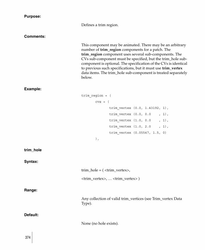
Purpose:
Defines a trim region.
Comments:
This component may be animated. There may be an arbitrary number of trim_region components for a patch. The trim_region component uses several sub-components. The CVs sub-component must be specified, but the trim_hole sub-component is optional. The specification of the CVs is identical to previous such specifications, but it must use trim_vertex data items. The trim_hole sub-component is treated separately below.
Example:
trim_region = (
cvs = (
trim_vertex (0.0, 1.43192, 1),
trim_vertex (0.0, 0.0 , 1),
trim_vertex (1.0, 0.0 , 1),
trim_vertex (1.0, 2.0 , 1),
trim_vertex (0.05547, 1.5, 0)
),
trim_hole
Syntax:
trim_hole = ( <trim_vertex>,
<trim_vertex>, … <trim_vertex> )
Range:
Any collection of valid trim_vertices (see Trim_vertex Data Type).
Default:
None (no hole exists).
374
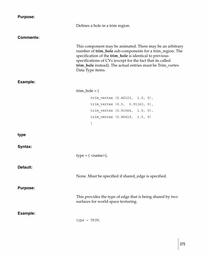
Purpose:
Defines a hole in a trim region.
Comments:
This component may be animated. There may be an arbitrary number of trim_hole sub-components for a trim_region. The specification of the trim_hole is identical to previous specifications of CVs (except for the fact that its called trim_hole instead). The actual entries must be Trim_vertex Data Type items.
Example:
trim_hole = (
trim_vertex (0.46123, 1.0, 0),
trim_vertex (0.5, 0.91163, 0),
trim_vertex (0.91564, 1.0, 0),
trim_vertex (0.86419, 1.5, 0)
)
type
Syntax:
type = ( <name>),
Default:
None. Must be specified if shared_edge is specified.
Purpose:
This provides the type of edge that is being shared by two surfaces for world-space texturing.
Example:
type = TRIM,
375
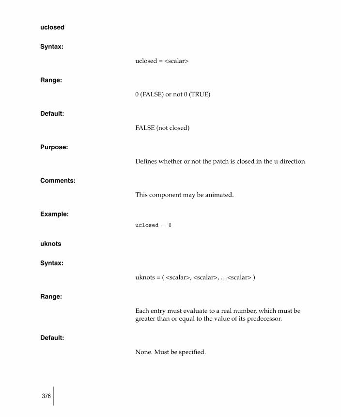
uclosed
Syntax:
uclosed = <scalar>
Range:
0 (FALSE) or not 0 (TRUE)
Default:
FALSE (not closed)
Purpose:
Defines whether or not the patch is closed in the u direction.
Comments:
This component may be animated.
Example:
uclosed = 0
uknots
Syntax:
uknots = ( <scalar>, <scalar>, …<scalar> )
Range:
Each entry must evaluate to a real number, which must be greater than or equal to the value of its predecessor.
Default:
None. Must be specified.
376
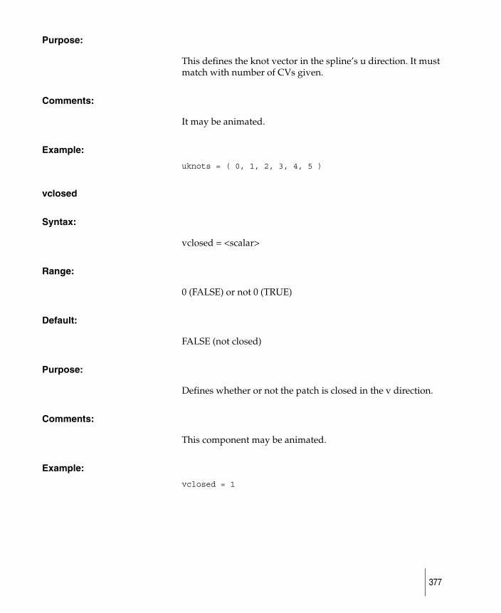
Purpose:
This defines the knot vector in the spline’s u direction. It must match with number of CVs given.
Comments:
It may be animated.
Example:
uknots = ( 0, 1, 2, 3, 4, 5 )
vclosed
Syntax:
vclosed = <scalar>
Range:
0 (FALSE) or not 0 (TRUE)
Default:
FALSE (not closed)
Purpose:
Defines whether or not the patch is closed in the v direction.
Comments:
This component may be animated.
Example:
vclosed = 1
377
vknots
Syntax:
vknots = ( <scalar>, <scalar>, …<scalar> )
Range:
Each entry must evaluate to a real number, which must be greater than or equal to the value of its predecessor.
Default:
None. Must be specified.
Purpose:
This defines the knot vector in the spline’s v direction. It must match with number of CVs given.
Comments:
This component may be animated.
Example:
vknots = ( -6.2, -5, -5, 0, 2.2, 2.2 )
udegree
Syntax:
udegree = <scalar>
Range:
1 to 33
Default:
none
378
Purpose:
To describe the degree of the nurbs curve in the u direction for patches. To define a syntactically correct curve, there must be at least degree + 1 control vertices.
Comments:
As the degree of the surface increases, it is a good idea to increase the rendering subdivisions for the object defined with that curve.
Example:
degree = 3
vdegree
Syntax:
vdegree = <scalar>
Range:
1 to 33
Default:
none
Purpose:
To describe the degree of the nurbs curve in the v direction for patches. To define a syntactically correct curve, there must be at least degree + 1 control vertices.
Comments:
As the degree of the surface increases, it is a good idea to increase the rendering subdivisions for the object defined with that curve.
379

Example:
degree = 3
380
Polyset Data Type
Syntax:
polyset <name> ( <component list> );
Reference:
<name>
Purpose:
A polyset is a polygonal mesh. It may be instanced as an object in the MODEL Section. A polyset may be specified as a literal or as a variable. If specified as a variable, it must have a name. Any of the following components may be specified between the parentheses:
● active
● casts_shadow
● clusters
● doublesided
● light_list
● motion_blur
● motion_blur_shading_samples
● motion_blur_texture_sample_level
● norm
● opposite
● particle_collisions
● polygon_areas
● polygon
● polygons
● shader
● smooth
● st
● texture_vertices
381
● vertex_normals
● vertices
Like a patch and a face, all components are specified using a keyword = value form. Components are separated by commas, and may be in any order. Not all components are optional. With the exception of the shader component, if components are specified multiple times, the last specification is used. Multiple shader components may be present in the polyset definition and be used by individual polygons. Components not specified take on their default value.
Example:
polyset Poly_1 (
active = ON,
motion_blur = ON,
smooth = ON,
doublesided = ON,
opposite = OFF,
shader = (DefaultShader ),
shader = (ShaderNumber2 ),
casts_shadow = TRUE,
vertices = ((cv((-11.89838, 4.210732, 0.0), 1)),
(cv((-2.174469, -7.479493, 0.0), 1)),
(cv((-13.28751, -8.289707, 0.0), 1)),
(cv((-2.174469, 6.409883, 0.0), 1)) ),
texture_vertices = (
st( 0.125000, 0.850394 ),
st( 1.000000, 0.055118 ),
st( 0.000000, 0.000000 ),
st( 1.000000, 1.000000 ) ),
vertex_normals = (
norm( 0.000000, 0.000000, 1.000000 ),
norm( 0.000000, 0.000000, 1.000000 ),
norm( 0.000000, 0.000000, 1.000000 ),
norm( 0.000000, 0.000000, 1.000000 ) ),
polygons = (
382
polygon ((0, 1, 2),(0, 1, 2),(0, 1, 2), 0 ),
polygon ((1, 0, 3),(1, 0, 3),(1, 0, 3), 1 )
)
); /* end of polyset ‘Poly_1’ */
active
Syntax:
active = <scalar>
Range:
0 (FALSE) or not 0 (TRUE)
Default:
TRUE
Purpose:
A Boolean flag that controls whether the polyset is visible or not.
Comments:
This component may be animated. This is provided so you no longer have to scale objects in an animation to 0 or translate them outside the scene for frames in which they shouldn’t appear.
Example:
active = FALSE
casts_shadow
Syntax:
casts_shadow = <scalar>
383
Range:
0 (FALSE) or not 0 (TRUE)
Default:
TRUE
Purpose:
A boolean that controls whether or not this polyset will cast a shadow.
Comments:
This component may be animated.
A surface with transparent or semi-transparent shading will not cast a shadow when RayCasting.
Example:
casts_shadow = FALSE
clusters
Syntax:
clusters = (<cluster matrix list>),
Range:
N/A
Default:
None.
Purpose:
A list of cluster matrices that affect the current surface.
384
Comments:
A cluster matrix describes the initial position of the matrix (4X4 scalars), the type of cluster effect (JOINT or LEAF), JOINT level (or 0 if the type is LEAF), and translate, rotate, scale as 3 scalar tuples.
Example:
clusters = (
clm( CL_r_peak,
1.0 , 0.0 , 0.0 , 0.0 ,
0.0 , 1.0 , 0.0 , 0.0 ,
0.0 , 0.0 , 1.0 , 0.0 ,
0.283681 , 0.0285822, -0.5841172, 1.0 ,
LEAF, 0,
0.0 , 0.0 , 0.0 ,
0.0 , 0.0 , 0.0 ,
1.0 , 1.0 , 1.0 ),
clm( CL_knot45_section0_Rwrist,
1.0 , 0.0 , 0.0 , 0.0 ,
0.0 , 1.0 , 0.0 , 0.0 ,
0.0 , 0.0 , 1.0 , 0.0 ,
0.283681 , 0.0285822, -0.5841172, 1.0 ,
LEAF, 0,
0.0 , 0.0 , 0.0 ,
0.0 , 0.0 , 0.0 ,
1.0 , 1.0 , 1.0 )
clm( CL_cluster#10,
1.0 , 0.0 , 0.0 , 0.0 ,
0.0 , 1.0 , 0.0 , 0.0 ,
0.0 , 0.0 , 1.0 , 0.0 ,
0.283681 , 0.0285822, -0.5841172, 1.0 ,
JOINT, 3,
-0.2398842, -0.0303474, 0.0 ,
0.0 , 0.0 , 0.0 ,
385
1.0 , 1.0 , 1.0 ) ),
doublesided
Syntax:
doublesided = <scalar>
Range:
0 (FALSE) or not 0 (TRUE)
Default:
TRUE; that is, the patch will be doublesided.
Purpose:
The scalar will be interpreted as a Boolean, with 0 being FALSE and any other value TRUE. If doublesided is FALSE, rendering proceeds more quickly, but only one side of the surface is rendered. For most objects other than closed surfaces, doublesided = TRUE is desirable. The reader is warned that with the raytracer, rays may strike the object from any direction.
Comments:
This component may be animated.
Example:
doublesided = FALSE
light_list
Syntax:
light_list = ( <light>, <light>, … <light> )
386
Range:
Each light given must have been defined; literals may not be used.
Default:
See below.
Purpose:
Each item referenced must be the name of a previously declared light data item, or an array element of type light (see the Light Data Type for more information). Literals may not be used. This lists the lights to be used by this polyset. If light_list is omitted or if it is specified and is empty, all nonexclusive lights are used to illuminate the polyset. If light_list is specified, and the list contains defined lights, then all instances of those lights in the scene, and only those, will be used for this polyset. This enables situations where you may want 10 lights on a particular object, for example, but only two lights on the rest of the scene.
Comments:
This component may not be animated.
Example:
light_list = ( spot01, spot02, flood, globallight )
motion_blur
Syntax:
motion_blur = <scalar>
Default:
ON
387
Range:
0 (OFF) or non-zero (ON)
Purpose:
If motion_blur_on is set for the file, this flag indicates that motion blur should be calculated for this object.
Example:
motion_blur = ON
motion_blur_shading_samples
Syntax:
motion_blur_shading_samples = <scalar>
Default:
3 - for bump or displacement mapped objects
1 - for all other objects
Range:
>= 3 for bump or displacement mapped objects
> 0 for all other objects
Purpose:
If motion_blur_on is set for the file, this flag indicates the number of samples done for shading of motion-blurred objects.
Example:
motion_blur_shading_samples = 1
388
motion_blur_texture_sample_level
Syntax:
motion_blur_texture_sample_level = <scalar>
Default:
3
Range:
0-5
Purpose:
If motion_blur_on is set for the file, this flag indicates the level of sampling done for texturing of motion-blurred objects. A 0 indicates no extra samples (lowest quality) and 5 means highest quality motion-blurred textures. Note, this flag does not apply to bump or displacement mapping.
Example:
motion_blur_texture_samples = 3
norm
Syntax:
norm( <scalar>, <scalar>, <scalar> )
Purpose:
Part of a polyset vertex normal list. The 'norm()' specifies the vertex normal coordinate.
Example:
norm( 0.000000, 0.000000, 1.000000 )
389
opposite
Syntax:
opposite = <scalar>
Range:
0 (FALSE) or not 0 (TRUE)
Default:
FALSE
Purpose:
To reverse the sense of direction of the normal for the polyset.
Comments:
This component may be animated. If doublesided is FALSE (for example, for faster execution), opposite can be used to reverse the orientation of the backfacing and frontfacing parts of the polyset. This may be done in order to correct potential visibility problems.
Example:
opposite = TRUE
particle_collisions
Syntax:
particle_collisions = BOUNDING_BOX_COLLISIONS | OFF | GEOMETRY_COLLISIONS
Range:
As above
390
Default:
OFF
Purpose:
To define which objects collide with particles.
Example:
particle_collisions = BOUNDING_BOX_COLLISIONS
polygon_areas
Syntax:
polygon_areas = ( <scalar>, ... <scalar>)
Default:
none
Purpose:
A list of areas, one per polygon, to be used in particle emission calculations.
Comments:
This component may not be animated. As particle emission rates depend on the area of a polygon, the area list component allows the initial areas of polygons to be set and made constant. The area list is indexed by the polygon number, so that polygon 0 in the polyset would use the first element of the area list.
Example:
polygon_areas = ( 0.2, 0.3, 2.4 )
391
polygon
Syntax:
polygon( (<integer>, <integer>, <integer>), [(<integer>, <integer>, <integer>),] [(<integer>, <integer>, <integer>)] [, <integer>])
Purpose:
Part of a polyset declaration. The integers represent indexes into the vertex, texture vertices, and vertex normals arrays that must accompany a polyset declaration. Additionally, the last parameter indicates which shader of those specified in the shader declarations should be used for this polygon.
Example:
polygon ((0, 1, 2),(3, 4, 5),(6, 7, 8), 0 )
The above example indicates that the polygon should use vertices number 0, 1, and 2 for position, texture vertices number 3, 4, and 5 for texture coordinates, and vertex normals 6, 7, and 8 for normals.
The trailing 0 indicates that the first shader declared in the polyset should be used to shade the polygon.
Note that the texture vertex and vertex normal data is optional. If the texture vertex information is not specified then 0, 0 will be used as texture coordinates. If the vertex normal data is not specified (and the vertex_normals list is not specified in the polyset), then the normals will be computed prior to rendering.
polygons
Syntax:
polygons = ( <polygon>, <polygon>, ... <polygon )
Range:
Any list of valid polygons.
392
Default:
None. Must be specified.
Purpose:
To describe the connectivity of previously declared vertices in the polyset.
Example:
polygons = (
polygon ((0, 1, 2), (0, 1, 2), (0, 1, 2), 0)
polygon ((1, 3, 4), (1, 3, 4), (1, 3, 4), 1)
)
shader
Syntax:
shader = (<shader>)
or
shader = ( <shader>, <shader>, … <shader> )
Range:
The shaders given may be variables or array elements of type shader (see Shader Data Type for more information). Note that there is no such thing as a literal shader.
Default:
None. Must be specified.
Purpose:
This specifies which shading characteristics are assigned to the surface.
393
Comments:
This component may be animated. If a list of shaders is specified, they will be visible in the order given.
Note also that multiple occurrences of the shader component may occur in a polyset definition. This allows multiple shaders to be assigned to the polyset. The shader used for any given polygon is specified as part of the polygon definition.
Example:
shader = (pink)
shader = (blue)
smooth
Syntax:
smooth = <scalar>
Range:
0 (OFF) or not 0 (ON)
Default:
ON
Purpose:
To enable the user to smooth or flat shade a polyset.
This component is animatable.
Example:
smooth = ON
394
st
Syntax:
st( <scalar>, <scalar> )
Purpose:
Part of a polyset texture vertex list. The 'st()' specifies the texture coordinate.
Example:
st( 0.34, 0.322 )
texture_vertices
Syntax:
texture_vertices = ( <st>, ... [<st>] )
Range:
Any collection of valid polyset texture vertices.
Default:
None. Must be specified.
Purpose:
Defines the texture vertex array for the polyset. The first texture vertex encountered is considered texture vertex 0 for the purposes of the polygon indices later in a polyset declaration, the second texture vertex encountered is considered vertex 1, and so on..
Comments:
This component must be specified before the 'polygons' component.
Example:
395
texture_vertices = (
st( 0.125000, 0.850394 ),
st( 1.000000, 0.055118 ),
st( 0.000000, 0.000000 ),
st( 1.000000, 1.000000 ) ),
vertex_normals
Syntax:
vertex_normals = ( <normal>, [<normal>] )
Range:
Any collection of valid polyset vertex normals.
Default:
None. Must be specified.
Purpose:
Defines the vertex normal array for the polyset. The first vertex normal encountered is considered vertex normal 0 for the purposes of the polygon indices later in a polyset declaration, the second vertex normal encountered is considered vertex normal1, and so on..
Comments:
This component must be specified before the 'polygons' component.
Example:
vertex_normals = ( norm( 0.000000, 0.000000, 1.000000 ), norm( 0.000000, 0.000000, 1.000000 ), norm( 0.000000, 0.000000, 1.000000 ), norm( 0.000000, 0.000000, 1.000000 ) ),
396
vertices
Syntax:
vertices = ( (<cv> [, <st>] [, <norm>]), (<cv> [, <st>] [, <norm>]), ... (<cv> [, <st>] [, <norm>]) )
Range:
Any collection of valid polyset vertices.
Default:
None. Must be specified.
Purpose:
Defines the vertex array for the polyset. The first vertex encountered is considered vertex 0 for the purposes of the polygon indices later in a polyset declaration, the second vertex encountered is considered vertex 1, and so on.
In version 7, it is now also possible to write the vertex normals and texture coordinates in separate lists of items, and index them separately by polygons. Because of this, StudioTools no longer places texture coordinates in the vertex definitions, though compatibility is maintained for older SDL files using this format.
Comments:
This component must be specified before the 'polygons' component. The <cv>s and <st>s are implicitly paired by the syntax, and this pairing is maintained.
Example:
vertices = ((cv((-11.89838, 4.210732, 0.0), 1)),
(cv((-2.174469, -7.479493, 0.0), 1)),
(cv((-13.28751, -8.289707, 0.0), 1)),
(cv((-2.174469, 6.409883, 0.0), 1)) ),
397
The equivalent of this example with vertex normals and texture coordinates is:
vertices = ((cv(( 0.0 , -0.5 , 0.0 ), 1.0 ), st( 0.0 , 0.0 ), norm (1.0, 0.0, 0.0)), etc...
398
Scalar Data Type
Declaration:
scalar <name> ( <expression> );
Reference:
<name>
Literal:
( <expression> )
or
<expression>
Purpose:
A scalar may be specified as a literal or as a variable. If specified as a variable, it must have a name. The only component of a scalar is its value.
Example:
scalar switch(OFF);
In version 7, to allow for faster processing and reduced SDL file sizes, animation curves that exhibit constant values will be written out as scalar values, not animation curves.
399
Shader Data Type
Declaration:
shader <name> ( procedure=<procedure name>, <component list> ) ;
Reference:
<name>
Purpose:
This defines a shader. A shader may only be specified as a variable, thus a name is always required. Any of the following components may be specified between the parentheses. Please note that particle system components are described in the section following the Light Data Type.
● bump
● color
● diffuse
● displacement
● eccentricity
● fill_color
● glow_intensity
● glow_rotation
● hide_glow_source
● incandescence
● matte_fraction
● model
● opacity_depth
● psys_bend_u
● psys_bend_v
● psys_blob_lighting
● psys_blob_map
400

● psys_blob_noise
● psys_blob_noise_frequency
● psys_blob_threshold
● psys_blur_quality
● psys_branch_angle
● psys_buoyancy
● psys_collisions
● psys_color
● psys_curl
● psys_density
● psys_elasticity
● psys_emission
● psys_end_frame
● psys_filename
● psys_friction
● psys_glow_intensity
● psys_hair_length_max
● psys_hair_length_min
● psys_hair_stiffness
● psys_hair_segments
● psys_hit_method
● psys_incandescence
● psys_lifespan_min
● psys_lifespan_max
● psys_mass
● psys_motion_type
● psys_num_children
● psys_parent_shading
● psys_particles_per_sec
● psys_randomization
● psys_render_type
401
● psys_size
● psys_speed
● psys_speed_decay
● psys_speed_range
● psys_split_time
● psys_start_frame
● psys_surface_shading
● psys_time_random
● psys_translucence
● psys_transparency
● psys_use_particle_file
● reflect_background
● reflection
● reflection_limit
● reflectivity
● refraction_jitter
● refraction_limit
● refraction_samples
● refractive_index
● respect_reflection_map
● shading_map
● shadow_level_limit
● shinyness
● specular
● specular_rolloff
● split_velocity_min
● surface_width
● translucence
● translucence_depth
● transparency
● transparency_shade
402
● u_patch_lines
● use_background_color
● use_fill_color
● v_patch_lines
Comments:
All components are specified using a keyword=value form. Components are separated by commas. Not all components are optional. The components may be specified in any order. Components that are not specified take on their default value. If any component is specified more than once, the last such specification will be used, and all previous ones ignored. If all are omitted, the defaults will result in a shader with the same properties as the interactive package default shader. Not all components are meaningful in all combinations. In situations where a component is not meaningful, any specification of it will be ignored with no ill effect.
Note that shaders cannot be used as literals.
Example:
shader arrow ( model = phong,
specular = (0.853881, 0.853881, 0.853881),
shinyness = 23.0,
color = (255.0, 0.0, 33.0)
);
bump
Syntax:
bump = texture <texture>
Range:
Not meaningful.
403
Default:
none.
Purpose:
The surface normal is perturbed according to the value given by the texture. Bump mapping makes a surface appear bumpy or rough by affecting the surface normal at a point and not by moving the actual surface. Therefore, the silhouette of the object will appear the same as it did before the bump map was applied. The scale of bumps is set by the amult and aoffset statements.
Comments:
This component may be animated. bump is appropriate for all shading models.
Example:
bump = noisy
color
Syntax:
color = <triple>
or
color = texture <texture>
Range:
Each component of a triple must be in the range 0 to 255.
Default:
( 0.0, 150.0, 255.0 )
404
Purpose:
If color = <triple>, the three components of the triple are the red, green and blue aspects of the color. If color = texture <texture>, then the texture is mapped onto the surface. A color is appropriate for all shading models. For more information on textures, see Texture Data Type.
Comments:
This component may be animated. Note that the default has been changed to agree with the interactive package.
Example:
color = (255.0, 0.0, 33.0)
diffuse
Syntax:
diffuse = <scalar>
Range:
Not checked; useful range is 0.0 to 1.0. While 0.0 to 1.0 provides a realistic range, numbers greater than 1 can be used: the effect is that more illumination is scattered by the object than was received by it.
Default:
0.8
Purpose:
The scalar determines the amount of illumination reflected by a matte surface, affecting the surface’s brightness. A high diffuse setting produces a broad range of shade on the object. A setting of 0.0 produces virtually no response to lights, while 1.0 produces very abrupt changes in shading, as found on acrylic or Plexiglass.
405
A diffuse component is appropriate for the lambert, phong, and blinn shading models. It is ignored for the lightsource model.
Comments:
This component may be animated.
Example:
diffuse = 0.99
displacement
Syntax:
displacement = texture <texture>
Range:
Not meaningful.
Default:
none.
Purpose:
The rendered surface is displaced along the surface normal according to the value given by the texture. With displacement maps, the silhouette is consistent with the rest of the surface, unlike bump maps.
Comments:
This component may be animated. displacement is appropriate for all shading models.
Example:
displacement = noisy
406
eccentricity
Syntax:
eccentricity = <scalar>
Range:
Any value other than 1.0
Default:
0.3
Purpose:
This is used only with the blinn shading model. It sets the size of the object’s highlight in a manner similar to the shinyness statement. This value controls the variance in the angle of the microfacets of the surface.
The eccentricity component should be specified for the blinn shading model. An eccentricity value of 0.0 is acceptable.
Comments:
This component may be animated.
Example:
eccentricity = 0.75
fill_color
Syntax:
fill_color= <triple>
Range:
Each component of a triple must be in the range 0 to 255.
407
Default:
(255, 255, 255)
Purpose:
Fill_color is only relevant in hidden-line rendering, and when use_fill_color is turned on. The fill color defines the interior color of the surface not covered by the outline of the surface.
Example:
fill_color= (255, 255, 255)
glow_intensity
Syntax:
glow_intensity = <scalar>
Range:
Non-negative
Default:
0.0
Purpose:
This simulates the effect when light intensity exceeds the range of the recording medium (e.g. film or a retina) causing light to bleed across the medium. Do to the limited contrast range of video and even film. it is impossible for something to appear very bright if it does not have a glowing halo. The glow fools our eyes into believing that the light is brighter than it really is.
Comments:
The glow intensity scales the intensity of a shaded pixel before it is passed into the post process glow pass. This intensity can not be greater than (255,255,255). For very bright
408
glows, the glow and halo color parameters in the ENVIRONMENT Section should be set high. Note that most of the parameters controlling shader glow are on the Environment. Components of shading (such as specular highlights or texture mapped dots) can be made to glow by using the threshold parameter on the Environment.
This component may be animated.
Example:
glow_intensity = .5
glow_rotation
Syntax:
glow_rotation = <scalar> (in degrees)
Range:
-infinity to infinity
Default:
0.0
Purpose:
To rotate the various glow and fog noise and star effects about the location of the shader.
Comments:
Affects glow_star_level, and glow_radial_noise.
Example:
glow_rotation = 45.0
409
hide_glow_source
Syntax:
hide_glow_source= <boolean>
Range:
ON or OFF.
Default:
OFF
Purpose:
This allows an object to be used as a source of glow without the object appearing in the final render: if this is ON then only the glow effect itself will appear. This is very useful when creating glowing gas like effects.
Comments:
If the glow_intensity is zero, hide_glow_source has no effect.
This component may be animated.
Example:
hide_glow_source = ON
incandescence
Syntax:
incandescence = <triple>
or
incandescence = texture <texture>
410
Range:
Each component of the triple must be in the range 0 to 255.
Default:
( 0.0, 0.0, 0.0 )
Purpose:
incandescence can be used for surfaces that appear to radiate energy, such as light bulbs and fire, and in moderate amounts for foliage. The value of incandescence is added to the color of the model. The effect is as if the model were glowing or radiating energy. incandescence is appropriate for all shading models.
Comments:
This component may be animated.
Example:
incandescence = (255.0, 0.0, 33.0)
matte_fraction
Syntax:
matte_fraction = <float>
Range:
0 to 1.
Default:
0.0
Purpose:
matte_fraction is only relevant when mask files are written during rendering. For each alpha value, (1-matte_fraction) is
411

multiplied to it to arrive at the actual alpha value written to file. This allows for opaque objects to not register an alpha, or allow an object (after compositing) to slowly become visible as you animate the matte_fraction from 1 to 0.
Comments:
This component may be animated.
Example:
matte_fraction = 0.0
model
Syntax:
Either : model = blinn
or: model = lambert
or: model = lightsource
or: model = phong
Range:
As enumerated above.
Default:
lambert
Purpose:
Sets the shading model used for rendering. The models are listed below in the order of their increasing sophistication and time required to render.
412
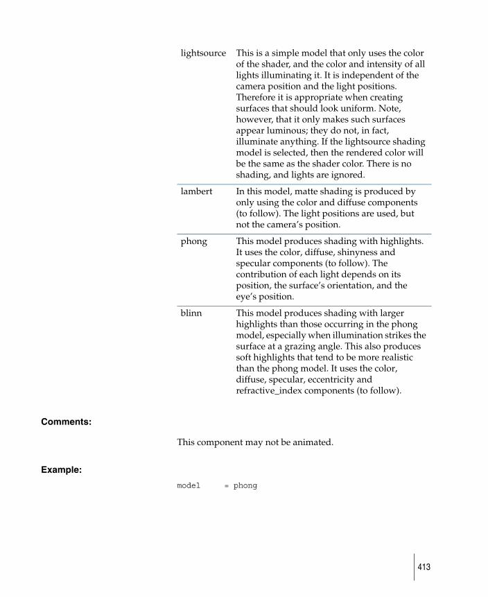
Comments:
This component may not be animated.
Example:
model = phong
lightsource This is a simple model that only uses the color of the shader, and the color and intensity of all lights illuminating it. It is independent of the camera position and the light positions.Therefore it is appropriate when creating surfaces that should look uniform. Note, however, that it only makes such surfaces appear luminous; they do not, in fact, illuminate anything. If the lightsource shading model is selected, then the rendered color will be the same as the shader color. There is no shading, and lights are ignored.
lambert In this model, matte shading is produced by only using the color and diffuse components (to follow). The light positions are used, but not the camera’s position.
phong This model produces shading with highlights. It uses the color, diffuse, shinyness and specular components (to follow). The contribution of each light depends on its position, the surface’s orientation, and the eye’s position.
blinn This model produces shading with larger highlights than those occurring in the phong model, especially when illumination strikes the surface at a grazing angle. This also produces soft highlights that tend to be more realistic than the phong model. It uses the color, diffuse, specular, eccentricity and refractive_index components (to follow).
413
opacity_depth
Syntax:
opacity_depth = <scalar>
Range:
Any floating point number.
Default:
0.0
Purpose:
Opacity depth causes transparency of an object to diminish with the thickness of an object. This is useful when creating hair, fur, and cloud effects. Objects will be fully opaque where their depth is greater than the opacity_depth. Note that when the opacity depth is zero, it has no effect (as opposed to making an object always opaque).
Comments:
The shader must have some transparency to view this effect. When opacity_depth is non-zero then transparency will modulate specularity, reflectivity, and incandescence, which are normally independent of transparency. This makes it easier to create soft fuzzy objects. Also, if you want to transparency map holes in a surface that has specular highlights, set the opacity_depth to a high value, instead of creating a matching specular map.
Transparent objects will cast shadows in the raycaster if their opacity depth is non-zero.
Example:
opacity_depth = 0.2
414

reflect_background
Syntax:
reflect_background = <scalar>
Range:
0 (OFF) or not 0 (ON).
Default:
OFF.
Purpose:
If the background has an environment map, then reflect_background = ON will reflect this environment.
Comments:
reflect_background overrides reflection mapping on the shader. It also overrides reflected rays in the RayTracer.
Example:
reflect_background = ON
reflection
Syntax:
reflection = texture <texture>
Range:
Not meaningful.
Default:
None (no reflection).
415
Purpose:
This provides a environment map for the current shader.
Comments:
This component may be animated. A reflection is appropriate for phong and blinn shading models.
Example:
reflection = room
reflection_limit
Syntax:
reflection_limit = <scalar>
Range:
Non-negative. If a negative number is given, zero will be used.
Default:
1
Purpose:
Ray tracing is a recursive process. Each ray bounces off of reflective objects. If the user places two reflective objects parallel to each other and places the eye point between them, then it is easy to imagine a ray bouncing back and forth between these mirrors forever. This is undesirable. The user can control the number of bounces a ray may take on a per shader basis with the reflection_limit component.
Comments:
This component may be animated.
Example:
reflection_limit = 0
416
Let us assume that an object uses a shader with this component. During the ray tracing process, a primary ray (which has a level of 0 by definition) hits this object. The reflectivity is calculated, and we prepare to trace a ray in the reflected direction. The reflection_limit is compared against the level of the incident ray. The reflected ray will be traced only if the reflection_limit is greater than the incident ray’s level. For the example this is false; the incident ray’s level is 0 and the reflection_limit is also 0. Therefore, no reflected ray is traced.
reflectivity
Syntax:
reflectivity = <scalar>
or
reflectivity = texture <texture>
Range:
unbounded, but meaningful range is 0.0 to 1.0
Default:
1.0
Purpose:
This scale factor is multiplied by the value produced by a reflection map. It allows the user to control the reflection map’s contribution to the final value of the shader. It is ignored if there is no reflection.
The reflectivity component is appropriate for the phong and blinn shading models. It is ignored for lightsource and lambert models. Also note that the reflection will be multiplied by specular, just like a highlight.
Comments:
This component may be animated.
417

Example:
reflectivity = 0.9
refraction_jitter
Syntax:
refraction_jitter= <scalar>
Range:
Between 0 and 1.
Default:
0
Purpose:
Refraction_jitter is valid for raytracing of transparent surfaces only. It jitters the refraction index for refraction rays. This can produce effects such as frosted glass. However, note that aliasing artifacts may arise when not enough refraction_samples are taken.
Example:
refraction_jitter= 0.1
refraction_limit
Syntax:
refraction_limit = <scalar>
Range:
Non-negative. If a negative number is given, zero will be used.
Default:
1
418
Purpose:
This controls the propagation of refracted rays through transparent objects. It is similar in intent and behavior to reflection_limit, but for refracted rays. It is only appropriate for RayTracing, and is ignored for all other modes of rendering.
Comments:
This component may be animated.
Example:
refraction_limit = 3
refraction_samples
Syntax:
refraction_samples= <scalar>
Range:
Any value greater than 1.
Default:
0
Purpose:
Refraction_samples defines the number of refraction rays to shoot when transparent surfaces are hit in ray tracing. This can achieve the effect of fuzzy refractions, and will also anti-alias refraction_jitter artifacts. Note that with a larger value specified for this parameter, the longer the ray tracing time.
Example:
refraction_samples= 1.1
419
refractive_index
Syntax:
refractive_index = <scalar>
Range:
Must be greater than 0.0; no maximum, but practical limit is 3.0.
Default:
1.3
Purpose:
This controls the angles of refracted rays through transparent objects. It is only appropriate for RayTracing, and is ignored for all other modes of rendering.
Example:
refractive_index = 3,
respect_reflection_map
Syntax:
respect_reflection_map = <scalar>
Range:
0 (FALSE) or not 0 (TRUE)
Default:
TRUE
Purpose:
This controls the use of a reflection map. RayTracing will reflect the environment of an object without having to create a
420
cubic or spherical reflection map (see Creating Rendered Cubic Environment Maps for more information on creating cubic reflection maps). There are times, however, that a user may want to use a reflection map rather than trace the reflected rays. For example, reflective pillars behind a complex car model are required to reflect the image of the car. RayTracing the reflections is expensive because of the sheer volume of geometry describing the car. Since the pillars are not the main focus of the rendering, the reflections on the pillars need not be all that accurate. Therefore, a reflection map may be used for the pillars with little quality degradation. Setting respect_reflection_map to TRUE will accomplish that. If this component is true, no reflection rays will be generated and any reflection map will applied. If respect_reflection_map is false and the rendering mode is raytrace, any reflection map will be ignored and reflection rays generated up to the relevant recursion limit. Note that this is only appropriate when RayTracing. Reflection maps are always applied when RayCasting.
Comments:
This component may be animated.
Example:
respect_reflection_map = FALSE
shading_map
Syntax:
shading_map= <triple>
or
shading_map= texture <texture>
Range:
Each component of a triple must be in the range 0 to 255.
421
Default:
( 0.0, 0.0, 0.0 )
Purpose:
If color = <triple>, the three components of the triple are the red, green and blue aspects of the color. If shading_map= texture <texture>, then u value of the texture is mapped to the shader’s hue, and the v value is mapped to the shader’s intensity. A color is appropriate for all shading models.
Comments:
This component may be animated. Note that the default has been changed to agree with the interactive package.
Example:
shading_map= (255.0, 0.0, 33.0)
shadow_level_limit
Syntax:
shadow_level_limit = <scalar>
Range:
-1 to infinity
Default:
1
Purpose:
This controls the propagation of shadow rays. It is similar in intent and behavior to reflection_limit, but for shadow rays. Shadow rays are generated towards all light sources with shadow = TRUE. Shadow rays are defined to be of the same level as the incident ray. Therefore, setting shadow_level_limit = 1; will cause shadow rays to be traced
422
from intersections generated by level 0 or level 1 rays. If a level 2 (or higher) ray strikes a object, no shadow rays will be traced, and the lighting will be calculated directly without shadowing. The shadow_level_limit component is only appropriate for RayTracing, and is ignored for all other modes of rendering.
Comments:
This component may be animated.
Example:
shadow_level_limit = 20
shinyness
Syntax:
shinyness = <scalar>
Range:
Must be greater than zero. Useful range is 2.0 to 200.0
Default:
20.0
Purpose:
This is used only with the phong shading model. The scalar determines the size of an object’s spot of reflection. The higher the value of the shinyness component, the smoother the surface looks. A shinyness component should be specified for the phong model.
Comments:
This component may be animated.
423
Example:
shinyness = 8
specular
Syntax:
specular = <triple>
or
specular = texture <texture>
Range:
Not checked; useful range is 0.0 to 1.0 for each of red, green and blue.
Default:
( 0.0, 0.0, 0.0 )
Purpose:
If specular = texture <texture>, the highlights across a surface can be made to vary. This requires a 24-bit map. If an 8-bit map is specified, a 24-bit greyscale map will be generated on the fly. You might use a texture here for such optical effects as gas on water or other iridescent effects. The triple is used as a multiplying factor for the red, green and blue aspects of the specular highlight. The multiplying factor affects the hue and the hotness or brightness of the specular highlight.
A specular component is appropriate for the phong and blinn shading models. It is ignored for lightsource and lambert models.
Comments:
This component may be animated. Note that the specular component affects reflected images (reflection maps) as well as highlights.
424
Example:
specular = (0.3, 0.4, 0.5)
specular_rolloff
Syntax:
specular_rolloff = <scalar>
Range:
Not checked; useful range is 0.0 to 1.0; absolute range is -infinity to infinity.
Default:
0.3
Purpose:
Controls the effect where some surfaces are more reflective at oblique angles. specular_rolloff has a range of 0.000 through 1.000. Rolloff values around 0.700 will create a “wet” look on a surface. specular_rolloff is only applicable to blinn model surfaces.
Also affects reflected rays in reflection maps.
Example:
specular_rolloff = 0.3,
split_velocity_min
Syntax:
split_velocity_min = <scalar>
Range:
0 to infinity
425

Default:
5
Purpose:
Appears only if psys_collisions are set to ON. This provides a limit on the speed a particle must be moving when it collides with an object to determine if the particle splits.
Example:
split_velocity_min = 5
surface_width
Syntax:
surface_width= <scalar>
Range:
Any value greater than 0.
Default:
0.0
Purpose:
Surface_width is only relevant in RayTracing for transparent surfaces. When the value is set to 0, the transparent surface is considered to be a solid. Thus refraction rays bend through this new medium in the interior of the surface. If a non-zero surface_width is specified, then the surface is not considered a solid, but rather the refraction rays bend through this new medium only for this surface width.
This is a fast method using RayTracing. Artifacts may appear if unreasonable surface_width values are specified (i.e. the surface width is actually larger than the surface itself).
426
Example:
surface_width= 0.3,
translucence
Syntax:
translucence = <scalar>
Range:
Any floating point number.
Default:
0.0
Purpose:
This simulates the way light diffusely penetrates through translucent objects. It is very useful for a wide range of materials: clouds, fur, hair, marble, jade, wax, paper, leaves, petals, frosted light bulbs. The translucence_depth determines the distanced light will penetrate into the object. If the translucence depth is greater than zero, then light can shine on surfaces that face away from the lightsource. For example, a spotlight with a texture map could act like a rear projector lighting up a translucent screen from behind. If the light casts shadows, then the translucence depth will determine how far the light can penetrate into the object.
Objects like fur and hair benefit greatly by shading the translucency and very little diffuse illumination. The effect is that small scale surface bumps and tufts have very soft shading as light readily passes through, while large scale features (like the back of the object, as opposed to the front) get full shadows and highlights. This effect is almost impossible to achieve without translucence.
Comments:
Note that for lights without shadowing, the translucence_depth is effectively zero or infinite (all non-zero
427
values). For raycast shadows, a faint gridlike artifact is sometimes visible. Usually this can be fixed by increasing the shadow quality or lowering the shadow resolution.
Generally it is useful to lower the diffuse intensity value when the translucence is high, to avoid washout.
The translucence calculation is based on illumination from lights, and has nothing to do with an object’s transparency; however, as an object becomes more transparent, the translucent (as well as diffuse) illumination gets dimmer.
Ambient lights have no effect on translucent (or diffuse) illumination.
This parameter may be animated.
Example:
translucence = 0.5
translucence_depth
Syntax:
translucence_depth = <scalar>
Range:
Any floating point number.
Default:
0.5
Purpose:
This determines how far light can translucently penetrate through an object.
See translucence for more information.
428
Comments:
Note that for lights without shadowing the translucence_depth is effectively zero or infinite (all non-zero values). In the raycaster, for very shallow depths (for example, 0.1) the spotlight parameter shadow_min_depth should be small (0.01) and the shadow_blend_offset should also be small (0.2).
This parameter may be animated.
Example:
translucence_depth = 0.2
transparency
Syntax:
transparency = <triple>
or
transparency = texture <texture>
Range:
0 to 255
Default:
0,0,0
Purpose:
Transparency is a three channel value. Any color can be specified as the transparency of a shader, white (255,255,255) being totally transparent and black (0,0,0) being totally opaque. Colors are filtered as you would expect; a white object behind a green transparent object will appear green (the red and blue having been filtered out), or a red object behind a blue transparent object will appear black.
If transparency is assigned a texture, the transparency across a surface can range from opaque to transparent depending on
429
the value of the texture at any point. If an 8 bit map is specified, the value of the map is repeated to make a color value; a value of 35 in the 8 bit map will become (35, 35, 35).
Note that highlights and reflections on very transparent objects will not be washed away. Transparency is appropriate for all shading models.
Comments:
This component may be animated.
Example:
transparency = (255, 255, 255)
transparency_shade
Syntax:
transparency_shade = <scalar>
Range:
0 to 1. If a number smaller than 0 is used, transparency_shade is forced to 0; for numbers greater than 1, transparency_shade is forced to 1.
Default:
0
Purpose:
Light is not equally shadowed when it passes through a transparent object: it is focused, creating illumination that is brighter at some points and darker at others. To produce this effect properly requires a special ray trace from the point of view of the light source, and it is expensive. In order to approximate this type of effect cheaply, we use a technique similar to the ambient light model. That is, light which passes nearly tangentially through a transparent object will be attenuated more than light passing nearly perpendicularly through it. This is controlled in the same manner as the
430
ambience component of an ambient light, but as part of the shader which is applied to the object.
Comments:
This component may be animated.
Example:
transparency_shade = 0
This results in a constant attenuation of the light through the object. With the default setting, planar transparent objects will cast a nearly uniform shadow unless a light source is close to the object.
u_patch_lines
Syntax:
u_patch_lines= <scalar>
Range:
Any value greater than 0.
Default:
0
Purpose:
U_patch_lines is only relevant in hidden-line rendering. By default, only the outline of the surface is drawn in hidden-line rendering (i.e. when u_patch_lines = 0). However, it is possible to get a gridded look of the outline, in which a number of lines per isoparm can be drawn through the u-direction of the surface. This number is the setting for u_patch_lines.
Because the gridded lines are drawn according to the uv-parameterization of the surface, it can warp undesirably. If such a case occurs, the best solution would be turn chord_length on in the texture definition.
431
Example:
u_patch_lines = 0
use_background_color
Syntax:
use_background_color = <scalar>
Range:
0 (OFF) to 1 (ON). If a number smaller than 0 is used, use_background_color is forced to 0; for numbers greater than 1, use_background_color is forced to 1.
Default:
0
Purpose:
For use_background_color, the color value for the shader is derived from the background. This may be used to apply shading to the background image or texture. Shadow and reflection catcher surfaces can be created with this method. It does not work in QuickRender. use_background_color overrides the shader color or color map value.
Example:
use_background_color = 0
use_fill_color
Syntax:
use_fill_color= <scalar>
432
Range:
0 (OFF) to 1 (ON). If a number smaller than 0 is used, use_fill_color is forced to 0; for numbers greater than 1, use_fill_color is forced to 1.
Default:
0
Purpose:
Use_fill_color is only relevant to hidden-line rendering. When turned off, only the outline of the objects are drawn in hidden-line rendering. When turned on, the interior of the surface is filled in with the color as specified by fill_color.
It must also be noted that when use_fill_color is turned off, the mask generated only shows the existence of the outline. When turned on, then the entire object’s mask value are assumed to be opaque.
Example:
use_fill_color = 0
v_patch_lines
Syntax:
v_patch_lines= <scalar>
Range:
Any value greater than 0.
Default:
0
Purpose:
V_patch_lines is only relevant in hidden-line rendering. By default, only the outline of the surface is drawn in hidden-line
433
rendering (i.e. when v_patch_lines = 0). However, it is possible to get a gridded look of the outline, in which a number of lines per isoparm can be drawn through the v-direction of the surface. This number is the setting for v_patch_lines.
Because the gridded lines are drawn according to the uv-parameterization of the surface, it can warp undesirably. If such a case occurs, the best solution would be turn chord_length on in the texture definition.
Example:
v_patch_lines = 0
434
Texture Data Type
Declaration:
texture <name> ( procedure=<procedure name>, <component list> ) ;
Reference:
<name>
Purpose:
This defines a texture. All textures are procedures, and, hence, the procedure name is required. Each procedure has its own set of components. However, all procedures have the following set of components in common:
● active
● amult
● aoffset
● aout
● blurmult
● bluroffset
● chord_length
● filter
● mirror
● offset
● repeat
● rotate
● rgbmult
● rgboffset
● rgbout
● scale
● translate
● wrap
435
● worldspace
Comments:
All components are specified using a keyword=value form.Components are separated by commas. Not all components are optional. The components may be specified in any order. Components which are not specified take on their default value. If any component is specified more than once, the last such specification will be used, and all previous ones ignored. Not all components are meaningful in all combinations. In situations where a component is not meaningful, any specification of it will be ignored with no ill effect.
Only those components common to all texture procedures are described here, See the description of the individual texture procedures for definition of the components unique to each. Note that texture components are not reserved words (and, thus, are not printed in bold here), although the terms texture and procedure both are reserved.
Example:
texture marb ( procedure = SmarbleRGB,
wrap = FALSE,
blurmult = 0.5
);
active
Syntax:
active
Range:
0 (FALSE) or not 0 (TRUE)
Default:
TRUE
436
Purpose:
active sets a flag indicating whether or not a given texture is to be used in the rendering process.
amult
Syntax:
amult = <scalar>
Range:
Generally, a useful range is from -1.0 to 1.0.
Default:
1.0
Purpose:
Value multiplier factor. All values of the texture are multiplied by this.
Comments:
This component may be animated.
The attribute being textured often has a limited range, so the value used for amult will have de facto limits in that context. For example, transparency is limited to the range 0 to 1. If an amult of -1 is used, then a corresponding aoffset must also be used to prevent the entire coverage area from bottoming out to zero.
Example:
amult = -1.0
437

aoffset
Syntax:
aoffset = <scalar>
Range:
A useful range is from -1.0 to 1.0.
Default:
0.0
Purpose:
Value offset factor. This is added to each value in the texture.
Comments:
This component may be animated.
Example:
aoffset = 1.0
aout
Syntax:
aout = <scalar>
Range:
0 to 1
Default:
0
438
Purpose:
Value outside of the area influenced by the texture.
Comments:
This component may be animated.
Example:
aout = 0.5
blurmult
Syntax:
blurmult = <scalar>
Range:
Non-negative. Generally, a useful range is from 0.0 to 10.0.
Default:
1.0
Purpose:
Scaling factor for blur of texture.
Comments:
This component may be animated.
Example:
blurmult = 0.2
bluroffset
Syntax:
bluroffset = <scalar>
439
Range:
Non-negative. Generally, a useful range is from 0.0 to 1.0.
Default:
0.0
Purpose:
Offset value for blur of texture.
Comments:
This component may be animated.
Example:
bluroffset = 0.001
chord_length
Syntax:
chord_length= <scalar>
Range:
0 (FALSE) to non-zero (TRUE)
Default:
FALSE
Purpose:
This flag maps a parametric texture so that it conforms to the curvature of the surface, not to the isoparametric surface values.
Example:
chord_length = TRUE;
440
filter
Syntax:
filter= <scalar>
Range:
0 (OFF), 1 (BLEND_FILTER), 2 (QUADRATIC_FILTER), 3 (QUARTIC_FILTER), 4(GAUSS_FILTER)
Default:
BLEND_FILTER
Purpose:
This flag selects a filter to use with file texture.
Example:
filter= BLEND_FILTER;
mirror
Syntax:
mirror
Range:
0 (FALSE) or not zero (TRUE)
Default:
FALSE
Purpose:
If mirror is TRUE, then repeated “tiles” of a texture are alternately flipped. Thus the colors at the seams will match, hiding the seams.
441
Comments:
This can be useful when trying to cover a large surface with a small texture sample. Note, however, that blur does not work across the seam when mirror = TRUE, and seams will appear between tiles if the texture is blurred.
For high quality seamless wrapping of textures, use the standalone “Fixwrap” on the source pix file instead of mirror. Fixwrap is included with alias_gifts. Type “fixwrap” without arguments for help information.
offset
Syntax:
uoffset = <scalar>,
voffset = <scalar>,
Range:
-∞ to ∞
Default:
0
Purpose:
uoffset and voffset determine the positioning of a texture within the coverage area.
Example:
uoffset = 0.989796, voffset = -0.3453,
repeat
Syntax:
urepeat = <scalar>,
442
vrepeat = <scalar>,
Range:
-∞ to 5
Default:
1
Purpose:
urepeat and vrepeat determine how many copies of the texture there are within the coverage area.
Example:
urepeat = -2.360882, vrepeat = 98.614067,
rotate
Syntax:
rotate = <scalar>,
Range:
-360 to 360
Default:
0
Purpose:
rotate is used to set the rotation (in degrees) of a texture on a shader.
Example:
rotate = 143.265305,
443
rgbmult
Syntax:
rgbmult = <triple>
Range:
Generally, a useful range for each component of the triple is from 0.0 to 1.0.
Default:
(1.0, 1.0, 1.0)
Purpose:
Provides a scaling factor for the value.
Comments:
This component may be animated.
The red, green, and blue components of the texture are multiplied by the numbers specified in the rgbmult triplet. The default of (1.0, 1.0, 1.0) means that all values are multiplied by 1, and are not changed. To darken the red component of a texture, reduce the first number. Using (0.5, 1.0, 1.0) results in the range for the red component being reduced to 0-128, and leaves the green and blue components at their full values. To increase the range of a component, use a number greater than 1. Be aware that you can’t get any brighter than 255 for each component.
Example:
rgbmult = ( sqrt(2), 1.0, 0.0 )
rgboffset
Syntax:
rgboffset = <triple>
444

Range:
A generally useful range for each component of the triple is from 0.0 to 255.0.
Default:
( 0.0, 0.0, 0.0 )
Purpose:
Offset for value. This is added to each value in the texture.
Comments:
This component may be animated.
Example:
rgboffset = ( 0.0, -128.0, 0.0 )
rgbout
Syntax:
rgbout = <triple>
Range:
Generally, a useful range for each component of the triple is 0.0 to 255.0.
Default:
( 0.0, 0.0, 0.0 )
Purpose:
Defines the value outside of the area influenced by the texture.
Comments:
This component may be animated.
445
Example:
rgbout = ( 255.0, 255.0, 255.0 )
scale
Syntax:
uscale = <scalar>
vscale = <scalar>
sx= <scalar>
sy= <scalar>
Range:
Non-negative.
Default:
1
Purpose:
The value assigned to uscale and vscale indicates the relative size of the texture map on the object 1 gives a full copy of the texture map. A scale of 0.5 means that the size of the texture map is double that of a scale of one: that is, only half of the texture map fits on the object. Scale is assigned in both u and v directions.
Sx and sy are only relevant to the Camera Type in Solid Projection. They store the scaling factors from the filmback space to image plane space.
translate
Syntax:
utranslate= <scalar>,
vtranslate = <scalar>,
446
tx= <scalar>,
ty= <scalar>,
Range:
-∞ to ∞
Default:
0
Purpose:
utranslate and vtranslate determine the placement of the area of coverage on a texture.
tx and ty are only relevant to the Camera Type in Solid Projection. They store the translation factors from the filmback space to image plane space.
Example:
utranslate = -3.511901, vtranslate = 1.0,
wrap
Syntax:
uwrap = <scalar>
vwrap = <scalar>
Range:
0 or 1
Default:
1 (ON = FALSE)
447
Purpose:
The value assigned to wrap indicates whether the texture will replicate itself over the entire surface in the either the u or v direction, or have only one copy of the texture mapped. To have a single copy in one direction on the surface, use 0 (off).
Comments:
This component may be animated.
Example:
wrap = FALSE
worldspace
Syntax:
worldspace = <scalar>,
Range:
0 or 1
Default:
1 (ON = TRUE)
Purpose:
worldspace sets a flag indicating whether a texture is to be rendered on a surface using worldspace texture mapping techniques.
448
Transformation Data Type
Declaration:
transformation <name>;
Reference:
<name>
Purpose:
The current transformation matrix is, in fact, a set of matrices that are maintained to relate the sense of position, orientation and size between objects and the world coordinate system. While the internal form of these (and their interdependencies) are not available to the user, it is convenient to be able to store, assign and use them. The transformation data type defines variables to do that.
There are no components of a transformation available to the user. A transformation may not be used as a literal.
Example:
transformation sticky;
449
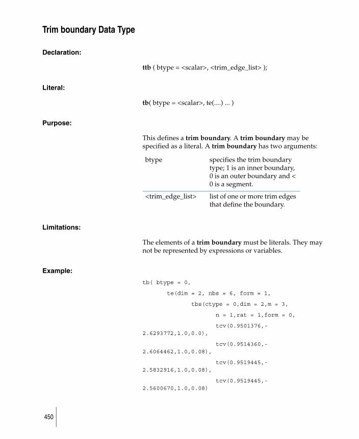
Trim boundary Data Type
Declaration:
ttb ( btype = <scalar>, <trim_edge_list> );
Literal:
tb( btype = <scalar>, te(....) ... )
Purpose:
This defines a trim boundary. A trim boundary may be specified as a literal. A trim boundary has two arguments:
Limitations:
The elements of a trim boundary must be literals. They may not be represented by expressions or variables.
Example:
tb( btype = 0,
te(dim = 2, nbs = 6, form = 1,
tbs(ctype = 0,dim = 2,m = 3,
n = 1,rat = 1,form = 0,
tcv(0.9501376,-2.6293772,1.0,0.0),
tcv(0.9514360,-2.6064462,1.0,0.08),
tcv(0.9519445,-2.5832916,1.0,0.08),
tcv(0.9519445,-2.5600670,1.0,0.08)
btype specifies the trim boundary type; 1 is an inner boundary, 0 is an outer boundary and < 0 is a segment.
<trim_edge_list> list of one or more trim edges that define the boundary.
450

)
)
)
451
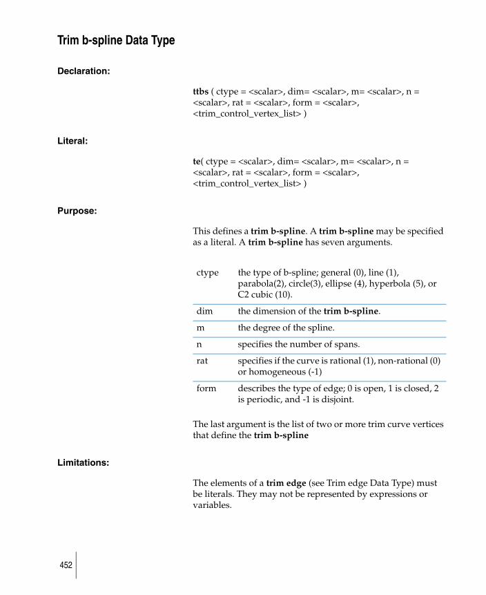
Trim b-spline Data Type
Declaration:
ttbs ( ctype = <scalar>, dim= <scalar>, m= <scalar>, n = <scalar>, rat = <scalar>, form = <scalar>, <trim_control_vertex_list> )
Literal:
te( ctype = <scalar>, dim= <scalar>, m= <scalar>, n = <scalar>, rat = <scalar>, form = <scalar>, <trim_control_vertex_list> )
Purpose:
This defines a trim b-spline. A trim b-spline may be specified as a literal. A trim b-spline has seven arguments.
The last argument is the list of two or more trim curve vertices that define the trim b-spline
Limitations:
The elements of a trim edge (see Trim edge Data Type) must be literals. They may not be represented by expressions or variables.
ctype the type of b-spline; general (0), line (1), parabola(2), circle(3), ellipse (4), hyperbola (5), or C2 cubic (10).
dim the dimension of the trim b-spline.
m the degree of the spline.
n specifies the number of spans.
rat specifies if the curve is rational (1), non-rational (0) or homogeneous (-1)
form describes the type of edge; 0 is open, 1 is closed, 2 is periodic, and -1 is disjoint.
452
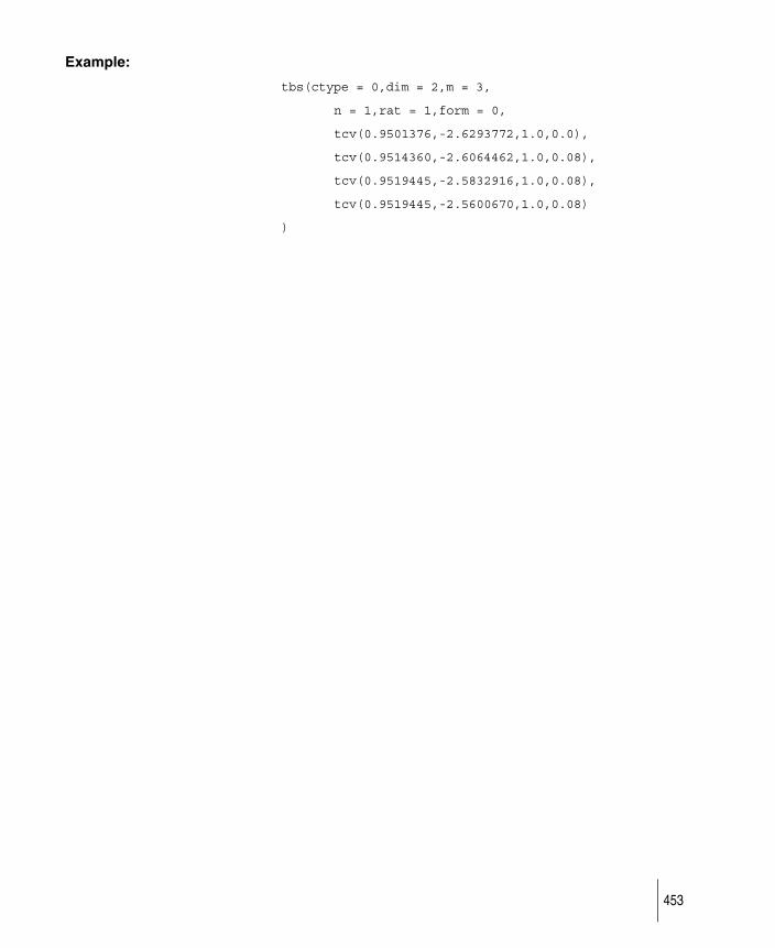
Example:
tbs(ctype = 0,dim = 2,m = 3,
n = 1,rat = 1,form = 0,
tcv(0.9501376,-2.6293772,1.0,0.0),
tcv(0.9514360,-2.6064462,1.0,0.08),
tcv(0.9519445,-2.5832916,1.0,0.08),
tcv(0.9519445,-2.5600670,1.0,0.08)
)
453
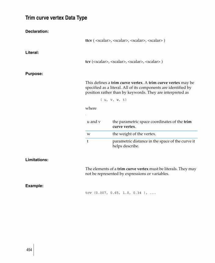
Trim curve vertex Data Type
Declaration:
ttcv ( <scalar>, <scalar>, <scalar>, <scalar> )
Literal:
tcv (<scalar>, <scalar>, <scalar>, <scalar> )
Purpose:
This defines a trim curve vertex. A trim curve vertex may be specified as a literal. All of its components are identified by position rather than by keywords. They are interpreted as
( u, v, w, t)
where:
Limitations:
The elements of a trim curve vertex must be literals. They may not be represented by expressions or variables.
Example:
tcv (0.007, 0.65, 1.0, 0.34 ), ...
u and v the parametric space coordinates of the trim curve vertex.
w the weight of the vertex.
t parametric distance in the space of the curve it helps describe.
454
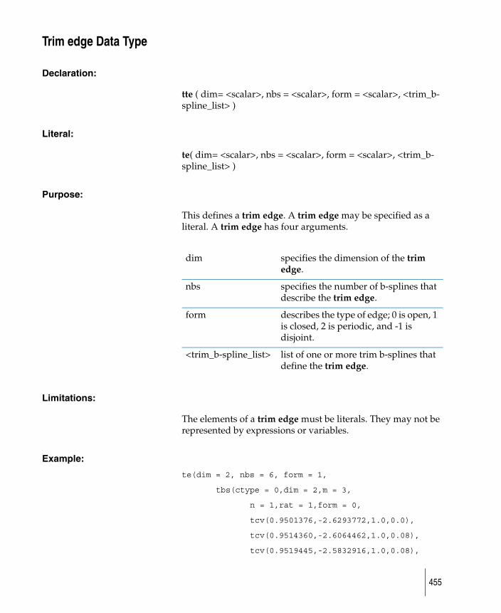
Trim edge Data Type
Declaration:
tte ( dim= <scalar>, nbs = <scalar>, form = <scalar>, <trim_b-spline_list> )
Literal:
te( dim= <scalar>, nbs = <scalar>, form = <scalar>, <trim_b-spline_list> )
Purpose:
This defines a trim edge. A trim edge may be specified as a literal. A trim edge has four arguments.
Limitations:
The elements of a trim edge must be literals. They may not be represented by expressions or variables.
Example:
te(dim = 2, nbs = 6, form = 1,
tbs(ctype = 0,dim = 2,m = 3,
n = 1,rat = 1,form = 0,
tcv(0.9501376,-2.6293772,1.0,0.0),
tcv(0.9514360,-2.6064462,1.0,0.08),
tcv(0.9519445,-2.5832916,1.0,0.08),
dim specifies the dimension of the trim edge.
nbs specifies the number of b-splines that describe the trim edge.
form describes the type of edge; 0 is open, 1 is closed, 2 is periodic, and -1 is disjoint.
<trim_b-spline_list> list of one or more trim b-splines that define the trim edge.
455
tcv(0.9519445,-2.5600670,1.0,0.08)
)
)
456
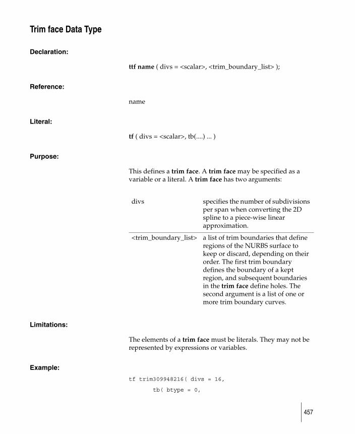
Trim face Data Type
Declaration:
ttf name ( divs = <scalar>, <trim_boundary_list> );
Reference:
name
Literal:
tf ( divs = <scalar>, tb(....) ... )
Purpose:
This defines a trim face. A trim face may be specified as a variable or a literal. A trim face has two arguments:
Limitations:
The elements of a trim face must be literals. They may not be represented by expressions or variables.
Example:
tf trim309948216( divs = 16,
tb( btype = 0,
divs specifies the number of subdivisions per span when converting the 2D spline to a piece-wise linear approximation.
<trim_boundary_list> a list of trim boundaries that define regions of the NURBS surface to keep or discard, depending on their order. The first trim boundary defines the boundary of a kept region, and subsequent boundaries in the trim face define holes. The second argument is a list of one or more trim boundary curves.
457
te(dim = 2, nbs = 6, form = 1,
tbs(ctype = 0,dim = 2,m = 3,
n = 1,rat = 1,form = 0,
tcv(0.9501376,-2.6293772,1.0,0.0),
tcv(0.9514360,-2.6064462,1.0,0.08),
tcv(0.9519445,-2.5832916,1.0,0.08),
tcv(0.9519445,-2.5600670,1.0,0.08)
)
)
)
);
458
Trim_vertex Data Type
Declaration:
trim_vertex <name> ( <scalar>, <scalar>, <scalar> ) ;
Reference:
<name>
Literal:
trim_vertex (<scalar>, <scalar>, <scalar> )
Purpose:
This defines a trim_vertex. A trim_vertex may be specified as a literal or as a variable. If specified as a variable, it must have a name. All of its components are identified by position rather than by keywords. They are interpreted as
( u, v, flag )
The meaning of u and v are the parametric space coordinates of the trim_vertex. The flag is interpreted as a Boolean. Zero (FALSE) means that this trim_vertex is interior to the surface it is associated with and trim curve algorithms should be used for processing it. Any other value (TRUE) means that this trim_vertex lies on the boundary of the surface and NURB curve algorithms should be used for processing it.
Limitations:
The elements of a trim_vertex must be literals. They may not be represented by expressions or variables.
Example:
trim_vertex nave (0.007, 0.65, 0 );
459
Triple Data Type
Declaration:
triple <name> ( <scalar>, <scalar>,<scalar> );
Reference:
<name>
Literal:
( <scalar>, <scalar>, <scalar> )
Purpose:
A triple may be specified as a literal or as a variable. If specified as a variable, it must have a name. The components of a triple are just the 3 values, which are identified by position rather than by keywords.
Example:
triple origin( 0, 0, 0 );
460
Using Data ItemsOnce a variable has been declared, it may be referenced. The reference to a variable may occur in the sense of retrieval, where the variable may be thought of as a source of values to be used. When referenced in this way, a variable behaves as though a corresponding literal had been used in place of the reference. This usage of variables is permitted anywhere in SDL, providing the variable being referenced has already been declared. Thus, it is possible to declare a <scalar>:
scalar max_color(255);
Then immediately use it to declare another variable, e.g.
triple white( max_color, max_color, max_color );
Indeed, this is exactly how normal use of SDL will proceed, with the declaration of basic building blocks followed by even larger pieces until all the items needed for the model have been defined. Thus, variables of the elementary data types (i.e., scalar, triple, CV, filename, shader, texture, array) will commonly be referenced as part of the declaration of other variables, or in the specification of literals. References to variables of the data types for “primitive objects” (i.e., light, patch, face) will normally be in the MODEL section of SDL where they will be used to create an instance of the object represented by the variable. Some of the data types provided in SDL are complex compositions of many components.
Some operations are defined for all data types, while other operations depend upon the data type. There are common operations which are allowed for variables of all data types except as noted below. These common operations are:
● a variable may be printed,
● a variable may be assigned the value of another variable of the same type,
● a variable may be assigned the value of an array element of the same type,
● a variable may be assigned the value of a literal of the same type,
● a variable may have its values assigned to another variable of the same type,
461
● a variable may have its values assigned to an array element,
● a variable may be referenced wherever a literal of the same type may be used.
An exception to the above is that there is no such thing as a literal (to serve as the source of an assignment) for some data types, namely: shaders and transformations. Note that printing means that the values of the components defining the variable will be output to “stderr”, not that some graphic rendition will be attempted. Note that operations on a scalar are the same as previous versions of SDL. This includes general usage in arithmetic expressions (see “expressions” below). While there is no such thing as a literal transformation, a variable of type transformation can have the current model transform assigned to it.
Arrays are special. While the above operations are valid and true for arrays, they don’t give the full picture. Therefore, the operations will be reconsidered here for arrays.
● An array may be printed. This means that each element in the array will be printed as though it were an independent variable.
● An array may have the contents of another array assigned to it. If the two arrays have the same number of elements, then the assignment takes place on an element by element basis. If the two arrays have a different number of elements, it is considered a syntax error, and execution terminated.
● A variable or a literal of any data type may be assigned to an array element. No checking of the array element’s previous contents is made, so the new value may be a different type from the previous.
● An array element may be used in place of a variable. The type of the present contents of the array element is considered the type of the element. That is, type checking of elements is performed at reference time (not assignment).
● Note that arrays have undefined element contents and undefined element types (unless an initial value is specified when the array is declared) until the element is given some value by assignment.
462

System Defined VariablesThere are some variables which are defined as part of the SDL. These variables are always defined, and may be referenced as desired. Their values are set and maintained automatically. In most cases (the exceptions will be noted), these variables may not be updated or changed by the user.
The majority of the variables correspond to the operational parameters. Those that do correspond have a default value, but may be set from command line arguments or by assignment in the DEFINITION section. Each variable is described below. System Defined Constants are described after the variables.
The following variables are described in this topic.
● aalevelmax
● aalevelmin
● aathreshold
● byframe
● endframe
● frame
● quiet
● startframe
● xleft
● xright
● yhigh
● ylow
aalevelmax
This variable corresponds to the operational parameter aalevelmax. It has a default scalar value of 2, but may be set from the -a command line option (see Command Line Options) or by assignment in the DEFINITION Section. It sets the maximum anti-aliasing level that will be used when rendering an image. Note that it may not be set by assignment (or by any other means) in any section except the DEFINITION section. See the description of DEFINITION
463
parameters for the meaning of this data and the values that it may take.
aalevelmin
It has a default scalar value of 1, but may be set by assignment in the DEFINITION Section. Note that it may not be set by assignment (or by any other means) in any section except the DEFINITION section. See the description of DEFINITION parameters for the meaning of this data and the values that it may take.
aathreshold
This variable corresponds to the operational parameter aathreshold. It has a default scalar value of 160, but may be set from the -t command line option (see Command Line Options) or by assignment in the DEFINITION Section. Note that it may not be set by assignment (or by any other means) in any section except the DEFINITION section. See the description of DEFINITION parameters for the meaning of this data and the values that it may take.
byframe
This variable corresponds to the operational parameter byframe. It has a default scalar value of 1, but may be set from the -b command line option (see Command Line Options) or by assignment in the DEFINITION Section. Note that it may not be set by assignment (or by any other means) in any section except the DEFINITION section. See the description of DEFINITION parameters for the meaning of this data and the values that it may take.
endframe
This variable corresponds to the operational parameter endframe. It has a default scalar value of 1, but may be set from the -e command line option (see Command Line Options) or by assignment in the DEFINITION Section. Note that it may not be set by assignment (or by any other means) in any section except the DEFINITION section. See the description of DEFINITION parameters for the meaning of this data and the values that it may take.
464
frame
This variable takes on scalar values from startframe to endframe at intervals of byframe during the rendering process. It may be thought of as the sense of time, or current “frame” within an animation. It need not be an integer value. It may not be modified by the user in any way, nor will its value ever be outside the specified range.
quiet
This variable corresponds to the operational parameter quiet. It has a default scalar value of FALSE, but may be set from the -q command line option (see Command Line Options) or by assignment in the DEFINITION Section. Note that it may not be set by assignment (or by any other means) in any section except the DEFINITION section. See the description of DEFINITION parameters for the meaning of this data and the values that it may take.
startframe
This variable corresponds to the operational parameter startframe. It has a default scalar value of 1, but may be set from the -s command line option (see Command Line Options) or by assignment in the DEFINITION Section. Note that it may not be set by assignment (or by any other means) in any section except the DEFINITION section. See the description of DEFINITION parameters for the meaning of this data and the values that it may take.
xleft
This variable corresponds to the operational parameter xleft. It has a default scalar value of 0, but may be set from the -x command line option (see Command Line Options) or by assignment in the DEFINITION Section. Note that it may not be set by assignment (or by any other means) in any section except the DEFINITION section. See the description of DEFINITION parameters for the meaning of this data and the values that it may take.
465
xright
This variable corresponds to the operational parameter xright. It has a default scalar value of 644, but may be set from the -w command line option (see Command Line Options) or by assignment in the DEFINITION Section. Note that it may not be set by assignment (or by any other means) in any section except the DEFINITION section. See the description of DEFINITION parameters for the meaning of this data and the values that it may take.
yhigh
This variable corresponds to the operational parameter yhigh. It has a default scalar value of 485, but may be set from the -h command line option (see Command Line Options) or by assignment in the DEFINITION Section. Note that it may not be set by assignment (or by any other means) in any section except the DEFINITION section. See the description of DEFINITION parameters for the meaning of this data and the values that it may take.
ylow
This variable corresponds to the operational parameter ylow. It has a default scalar value of 0, but may be set from the -y command line option (see Command Line Options) or by assignment in the DEFINITION Section. Note that it may not be set by assignment (or by any other means) in any section except the DEFINITION section. See the description of DEFINITION parameters for the meaning of this data and the values that it may take.
466
System Defined ConstantsLike the system defined variables, there are some constants which are defined as part of the SDL. These constants are always defined, and may be referenced as desired. Each is described below.
The following constants are defined in this section.
● FALSE
● OFF
● ON
● TRUE
● xaxis
● yaxis
● zaxis
FALSE
This is a constant with the scalar value of 0. It is useful when a constant truth value is desired. Note that the value is identical to the constant OFF, with which it is interchangeable.
OFF
This is a constant with the scalar value of 0. It is useful when a constant truth value is desired. Note that the value is identical to the constant FALSE, with which it is interchangeable.
ON
This is a constant with the scalar value of 1. It is useful when a constant truth value is desired.
Note that the value is identical to the constant TRUE, with which it is interchangeable.
467
TRUE
This is a constant with the scalar value of 1. It is useful when a constant truth value is desired. Note that the value is identical to the constant ON, with which it is interchangeable.
xaxis
This is a constant with the scalar value of 0. It is meant to describe one of the possible axes of rotation for use in the rotate statement. See the description of that statement for more information on the meaning of the possible axes.
yaxis
This is a constant with the scalar value of 1. It is meant to describe one of the possible axes of rotation for use in the rotate statement. See the description of that statement for more information on the meaning of the possible axes.
zaxis
This is a constant with the scalar value of 2. It is meant to describe one of the possible axes of rotation for use in the rotate statement. See the description of that statement for more information on the meaning of the possible axes.
468

ExpressionsThere are three types of expressions: Primary Expressions, Unary Operator Expressions and Binary Operator Expressions. These will be described in turn.
Functions are described in the next section.
Primary Expressions
Primary expressions may be further divided into five kinds:
1) Variables,
2) Array Elements,
3) Literals,
4) Function Calls, and
5) Parenthesized Expressions.
Array Elements
An array element may be used as an expression if 1) the subscript referencing it is in the range defined when the array was declared, and 2) the type of the element is scalar. Since the subscript itself may be a variable and the contents of an array element may be of any type, the test for the above conditions is made at reference time.
Function Calls
Only functions which return a scalar may be used as an expression. The syntax of a function call is:
<function name> ( <argument list> )
The contents of the argument list vary depending upon the function being invoked. The reader is referred to the detailed descriptions of the individual functions for the specification of the arguments required by each. Note that the argument list may be empty for some functions, but the delimiting parentheses are still required. As with “C”, function
469
arguments are passed by value, and the arguments themselves will not be affected in any way by the function call.
Literals
Only literals of type scalar may be used as an expression. The value given is used.
Parenthesized Expressions
A parenthesized expression consists of a left parenthesis, any expression, and then a right parenthesis — ( <expression> )
The purpose of the parenthesized expression is simply to delimit the enclosed expression for grouping purposes. Normally the enclosed expression will be a binary operator expression, although any type of expression is valid. The classic example is a grouping to defeat the normal precedence of operators with a binary operator expression — ( x + 1 ) / 2
Variables
Only variables of type scalar may be used as an expression. Since variables of that type always have a value defined, the use of a variable as an expression is just a reference to that value.
Unary Operator Expressions
Two unary operators are provided, logical negation ( ! ), and arithmetic negation ( – ). In both cases the syntax is:
<operator><primary expression>
where <operator> is either “!” or “-”. Any primary expression is valid, but only a primary expression. Logical negation results in a value for the expression of either 0 (FALSE) or 1 (TRUE). A value of 1 results when the <primary expression> has a value of zero. A value of 0 results when the <primary expression> has any other (non-zero) value. Arithmetic negation simply changes the sign of the value of the <primary expression>. Zero is unsigned and unaffected by this operator. Logical negation takes precedence over arithmetic negation.
470

Binary Operator Expressions
A binary operator expression consists of 2 expressions (of any kind) separated by a binary operator. There are 12 binary operators, which have 5 different levels of precedence, namely:
* /highest precedence
+ -
== != >= <= > <
&&
||lowest precedence
All binary operators have a lower precedence than the unary operators. All binary operators are left associative. The individual operators will be discussed in order of decreasing precedence.
Multiplication ( * ) and division ( / ) have the same precedence. All arithmetic is performed in single precision floating point form. Division by zero is invalid and results in a terminated execution. Addition ( + ) and subtraction ( – ) have the same precedence, which is lower than multiplication or division. The computation is performed in single precision floating point form.
The operators “<”, “>”, “<=”, “>=”, “==” and “!=” are collectively known as trelation operators. They represent “less than”, “greater than”, “less than or equal to”, “greater than or equal to”, “equality”, and “not equal”, respectively. All the relation operators have the same precedence. The relation operators compare the values of 2 expressions. The result of such a comparison is either 1 in the case where the specified relationship exists (the TRUE case) or 0 in the case where the relation does not exist (FALSE).
All comparisons are between single precision floating point numbers. The user is therefore advised to exercise care when using tests for equality. A second potential problem could occur because of the left associativity combined with all relation operators having the same precedence and the left to right evaluation order of expressions. The user is urged to use
471
explicit grouping whenever more than one relation operator is needed.
Consider, for example,
a > b > 3
This will always evaluate to 0 (FALSE), because the associativity results in
( a > b ) > 3
and the result of a > b must be either 1 or 0, neither of which is greater than 3.
The logical AND operator ( && ) interprets the two expressions as truth values and performs the logical intersection. An expression is considered true if its value is non-zero, and false if its value is zero. The result of the intersection is either 1 (in the case where the expressions are both true) or 0 (for all other cases). Note that the left expression is evaluated first, and if it is false then the result is determined and the right expression is not inspected at all. This behavior is similar to the “C” language and is sometimes useful when the value of an expression might not be well defined (as with arrays for instance).
The logical OR operator ( || ) interprets the two expressions as truth values and performs the logical union. An expression is considered true if its value is non-zero, and false if its value is zero. The result of the union is either 1 (in the case where either of the expressions are true) or 0 (in the case where both expressions are false). Note that the left expression is evaluated first, and if it is true then the result is determined and the right expression is not inspected at all. This behavior is similar to the “C” language and is sometimes useful when the value of an expression might not be well defined (as with arrays for instance).
472
FunctionsThere are a number of functions defined for SDL that may be used in an expression or in place of an expression. Most functions (there are a few exceptions) return a single (scalar) value. Most functions are simply routines from the standard UNIX math library. These will not be documented, defined, or described here. The reader is referred to the standard UNIX documentation. They are:
besselj0 besselj1 besseljn
besselyn
cos acos cosh
erf erfc
exp
fabs
floor ceil
hypot
log10
pow
sin asin sinh
sqrt
tan atan atan2 tanh
Some basic extensions to the trigonometric functions are provided so that angles may be expressed in degrees rather than radians:
cosd acosd
sind asind
tand atand atan2d
These are identical to the standard routines in all respects except that the angles are expressed in degrees.
473
In addition to the math library routines, SDL has the following functions defined:
animate
cl() [formerly cluster()]
constrain( )
current_position
current_transformation
ease
extract
fmod
gamma
motion
rand srand gauss
sign
Each of these is described in detail below.
animate
The animate function is used to define animated behaviors. It takes 2 arguments, and returns a scalar:
animate( <parameter_curve>, <time> )
The <parameter_curve> argument defines the parameter curve to be used for an animation. It must be the name of a <parameter_curve> variable defined in the definition section. The <time> argument specifies where along the curve to interpret the value. It is a scalar, and will normally be the system defined variable frame. The animate function returns a scalar. The value returned is the value of the <parameter_curve> at time <time>.
474
Example:
translate(animate( sphere.X_Position, frame ), 0.0, 0.0);
cl() [formerly cluster()]
Returns:
CV
Syntax:
cl( <cv>, <cluster_matrix_reference>, <percentage> [, <cluster_matrix_reference>, <percentage> ] )
The cl or cluster function takes <cv> and applies the specified clusters at the given percentages.
For a description of how clusters are applied to CVs, please check the animation section of the documentation.
Example:
cl(cv((-0.928135, -0.066296, 3.525111), 1.0),
CL_cluster#2 ,0.0,
CL_knot100_section270_Relbow ,0.003524,
CL_knot0_section270_Relbow ,0.879251,
CL_knot26_section0_Relbow ,0.007034,
CL_knot0_section0_Relbow ,0.462762) )
constrain( )
Syntax:
constrain ( start, end, by, constrain_value )
Constrain function takes 4 scalar arguments. The return value is constrained to be start, end, or (start + N * by) where (N * by) is not greater than (end - start). The start value must be less than the end value. If (constrain_value <= start) then start is returned. If (constrian_value >= end) then end is returned. If (by = 0), then the function will always return the start value.
475
This function is useful for animating visibility exactly, or turning a smooth curve into discrete steps.
Example:
The following function will return 19, because its possible return values are 13, 16, 19, 22, and 25.
x = constrain ( 13, 25, 3, 18 );
current_position
This function returns a triple value corresponding to the x, y, and z coordinates of a point in space defined in the model where the function is called. It takes a triple as an argument. Its value outside the MODEL section is undefined, and any references to it outside that section are invalid and will generate an error.
Example:
<triple_variable> = current_position( x, y, z );
or
<triple_variable> = current_position( motion(
<motion_path>, animate( <timing_curve>, frame )));
current_transformation
This function returns a transformation value corresponding to its placement in the modeling hierarchy. It does not take any arguments. It is used primarily to mark the location of a solid texture or a cluster. Its value outside the MODEL section is undefined, and any references to it outside that section are invalid and will generate an error.
Example:
<texture_orientation> = current_transformation();
ease
The ease function takes 5 arguments. It returns a scalar. It is used primarily for animation.
476
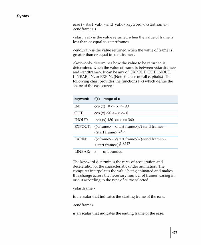
Syntax:
ease ( <start_val>, <end_val>, <keyword>, <startframe>, <endframe> )
<start_val> is the value returned when the value of frame is less than or equal to <startframe>.
<end_val> is the value returned when the value of frame is greater than or equal to <endframe>.
<keyword> determines how the value to be returned is determined when the value of frame is between <startframe> and <endframe>. It can be any of: EXPOUT, OUT, INOUT, LINEAR, IN, or EXPIN. (Note the use of full capitals.) The following chart provides the functions f(x) which define the shape of the ease curves:
The keyword determines the rates of acceleration and deceleration of the characteristic under animation. The computer interpolates the value being animated and makes this change across the necessary number of frames, easing in or out according to the type of curve selected.
<startframe>
is an scalar that indicates the starting frame of the ease.
<endframe>
is an scalar that indicates the ending frame of the ease.
keyword: f(x) range of x
IN: cos (x) 0 <= x <= 90
OUT: cos (x) -90 <= x <= 0
INOUT: -cos (x) 180 <= x <= 360
EXPOUT: ((<frame> - <start frame>)/(<end frame> - <start frame>))0.3
EXPIN: ((<frame> - <start frame>)/(<end frame> - <start frame>))1.8547
LINEAR: x unbounded
477
Example:
light(intensity=ease(1.0,0.0,LINEAR,startframe,endframe), color=(255,0,0));
extract
Allows individual channels of a triple to be extracted as scalars. Most useful for getting at the individual values of a motion path. Extract has two arguments, a scalar, which specifies the element to extract and a triple from which the element will be extracted. The first scalar argument must be one of (1, 2, 3) meaning return the first, second, or third scalar of the following triple.
This function returns a scalar.
Example
x = extract(1.0, motion(motion_path, animate(param_curve.Timing, frame)));
fmod
The fmod function takes 2 arguments. It returns a scalar, whose value is the floating point remainder of the division of the first argument by the second argument. If the divisor is zero, then an error is reported and execution terminated. The result will have the same sign as the dividend. Note that this is a custom built Animator function because not all UNIX systems provide it.
Example:
even = fmod(frame,2);
gamma
Given floating point output color (R, G, B), the user-supplied gamma_value, and the function “pow(X,Y)” which raises X to the power of Y, gamma in the renderer is applied:
R=255.0*pow((R/255.0), gamma_value);
G=255.0*pow((G/255.0), gamma_value);
478
B=255.0*pow((B/255.0), gamma_value);
/*Clip the value to 255.*/
if (R>255.0) R=255.0;
if (G>255.0) G=255.0;
if (B>255.0) B=255.0;
gauss
The gauss function does not take any arguments. (The syntax still requires that parentheses be included, however.) It returns a scalar whose value is a pseudo random number with a gaussian (normal) distribution. The random number function may be initialized by using the srand function to set the seed. If srand is not called, the default seed value will be used. See the description of srand for details. Note that even though the routines to compute random numbers are the same, the numbers returned may be different on different machines because of differences in the underlying hardware.
Example:
distrib = gauss();
motion
The motion function is used to define animated behaviors. It takes 2 arguments:
motion( <curve>, <distance> )
The <curve> argument defines a 3D curve to be used for an animation. It will be the name of a curve variable. The <distance> argument specifies where along the curve to interpret the value. It is a scalar, and specifies the parametric distance along the curve. The parametric distance is 0 at the end of the curve corresponding to the first CV and 1 at the end of the curve corresponding to the last CV. Normal usage of the motion function will relate the parametric distance to frame time by way of a nested animate. For example,
motion( some_path, animate( timing_curve, frame ))
479
The motion function returns a triple. The value returned is the point along the <curve> at <distance> from the end. If <distance> is outside the range 0 to 1, then the value of <curve> at one end or the other (the start if <distance> is less than 0, the end if <distance> is greater than 1) will be given.
rand
The rand function does not take any arguments. (The syntax still requires that parentheses be included, however.) It returns a scalar whose value is a pseudo random number uniformly distributed between -1.0 and 1.0. The random number function may be initialized by using the srand function to set the seed. If srand is not called, the default seed value will be used. See the description of srand for details. Note that even though the routines to compute random numbers are the same, the numbers returned may be different on different machines because of differences in the underlying hardware.
Example:
flake = rand();
sign
The sign function takes one argument. It returns a scalar with the value -1 if the argument is negative, 0 if the argument is 0, or +1 if the argument is positive.
Example:
if (sign(byframe)) print("infinite loop");
srand
The srand function takes one argument. It returns a scalar with the constant value 0. The argument provided will be used as the initial seed for random number generation. The argument should be a scalar. If the argument is omitted or of the wrong type, a warning message will be generated, the default seed value will be used, and execution will continue as if everything were correct. The default seed value is
12345.
480
Example:
bogus = srand(54321);
warp
The warp function is used to globally change the timing of animation parameters. It takes 2 arguments:
warp( <curve>, <time> )
The <curve> argument defines the parameter curve to be used for an animation. It will normally be a <parameter_curve> <parameter_vertex>s. The <time> argument specifies where along the curve to interpret the value. It is a scalar, and will normally be the system defined variable frame. The warp function returns a scalar. The value returned is the value of the <curve> at time <time>. If <time> is below the first specified value of the <curve>, the value returned is:
start_value - (start_value - <time>)
If <time> is greater than the last value, then the value returned is:
end_value + (<time> - end_value)
In other words, above (or below) the valid range for a warp function, the function increases (or decreases) linearly from the end (or start) values.
Example:
animate (“transZ.curve”, warp(“rotateX.curve”, warp(transY.curve”, frame)));
Please note that this function is obsolete.
481

482
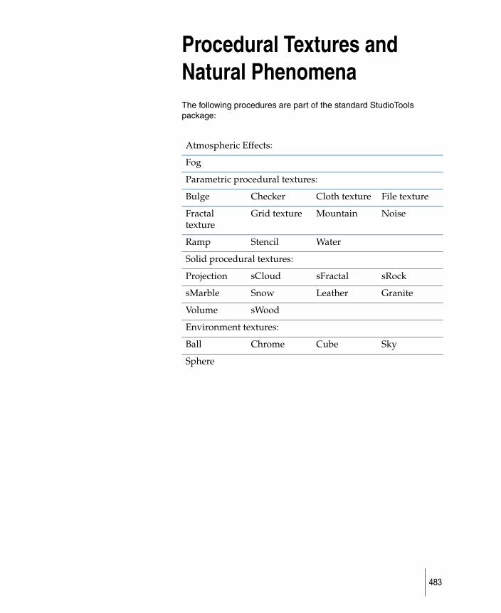
Procedural Textures and Natural PhenomenaThe following procedures are part of the standard StudioTools package:
Atmospheric Effects:
Fog
Parametric procedural textures:
Bulge Checker Cloth texture File texture
Fractal texture
Grid texture Mountain Noise
Ramp Stencil Water
Solid procedural textures:
Projection sCloud sFractal sRock
sMarble Snow Leather Granite
Volume sWood
Environment textures:
Ball Chrome Cube Sky
Sphere
483
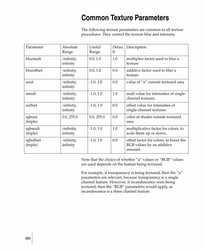
Common Texture ParametersThe following texture parameters are common to all texture procedures. They control the texture blur and intensity.
Note that the choice of whether “a” values or “RGB” values are used depends on the feature being textured.
For example, if transparency is being textured, then the “a” parameters are relevant, because transparency is a single channel feature. However, if incandescence were being textured, then the “RGB” parameters would apply, as incandescence is a three channel feature.
Parameter Absolute Range
Useful Range
Default
Description
blurmult -infinity, infinity
0.0, 1.0 1.0 multiplier factor used to blur a texture
bluroffset -infinity, infinity
0.0, 1.0 0.0 additive factor used to blur a texture
aout -infinity, infinity
-1.0, 1.0 0.0 value of “a” outside textured area
amult -infinity, infinity
-1.0, 1.0 1.0 mult value for intensities of single-channel textures.
aoffset -infinity, infinity
-1.0, 1.0 0.0 offset value for intensities of single-channel textures
rgbout (triple)
0.0, 255.0 0.0, 255.0 0.0 color of shader outside textured area
rgbmult (triple)
-infinity, infinity
-1.0, 1.0 1.0 multiplicative factor for colors, to scale them up or down.
rgboffset (triple)
-infinity, infinity
-1.0, 1.0 0.0 offset factor for colors, to boost the RGB values by an additive amount.
484
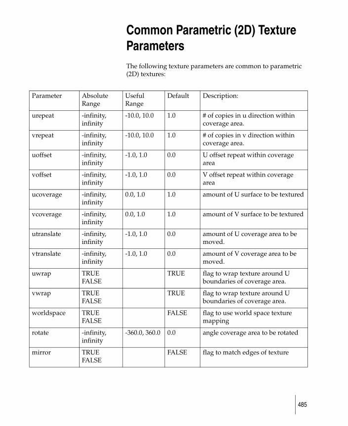
Common Parametric (2D) Texture ParametersThe following texture parameters are common to parametric (2D) textures:
Parameter Absolute Range
Useful Range
Default Description:
urepeat -infinity, infinity
-10.0, 10.0 1.0 # of copies in u direction within coverage area.
vrepeat -infinity, infinity
-10.0, 10.0 1.0 # of copies in v direction within coverage area.
uoffset -infinity, infinity
-1.0, 1.0 0.0 U offset repeat within coverage area
voffset -infinity, infinity
-1.0, 1.0 0.0 V offset repeat within coverage area
ucoverage -infinity, infinity
0.0, 1.0 1.0 amount of U surface to be textured
vcoverage -infinity, infinity
0.0, 1.0 1.0 amount of V surface to be textured
utranslate -infinity, infinity
-1.0, 1.0 0.0 amount of U coverage area to be moved.
vtranslate -infinity, infinity
-1.0, 1.0 0.0 amount of V coverage area to be moved.
uwrap TRUE FALSE
TRUE flag to wrap texture around U boundaries of coverage area.
vwrap TRUE FALSE
TRUE flag to wrap texture around U boundaries of coverage area.
worldspace TRUE FALSE
FALSE flag to use world space texture mapping
rotate -infinity, infinity
-360.0, 360.0 0.0 angle coverage area to be rotated
mirror TRUE FALSE
FALSE flag to match edges of texture
485

The parametric textures are: Bulge, Checker, Cloth texture, File texture, Fractal, Grid, Mountain, Noise, Ramp, Stencil, and Water.
486
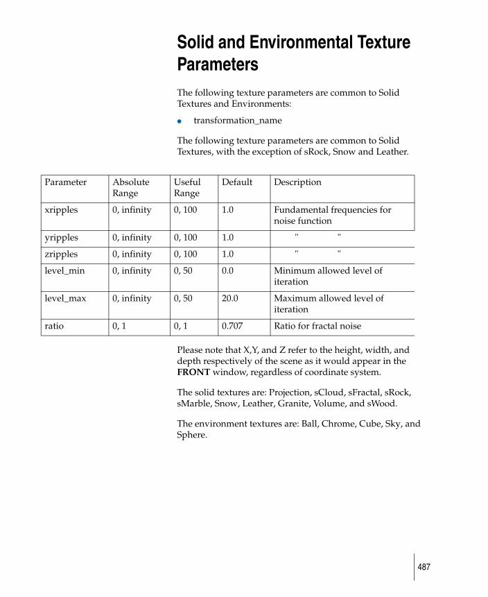
Solid and Environmental Texture ParametersThe following texture parameters are common to Solid Textures and Environments:
● transformation_name
The following texture parameters are common to Solid Textures, with the exception of sRock, Snow and Leather.
Please note that X,Y, and Z refer to the height, width, and depth respectively of the scene as it would appear in the FRONT window, regardless of coordinate system.
The solid textures are: Projection, sCloud, sFractal, sRock, sMarble, Snow, Leather, Granite, Volume, and sWood.
The environment textures are: Ball, Chrome, Cube, Sky, and Sphere.
Parameter Absolute Range
Useful Range
Default Description
xripples 0, infinity 0, 100 1.0 Fundamental frequencies for noise function
yripples 0, infinity 0, 100 1.0 " "
zripples 0, infinity 0, 100 1.0 " "
level_min 0, infinity 0, 50 0.0 Minimum allowed level of iteration
level_max 0, infinity 0, 50 20.0 Maximum allowed level of iteration
ratio 0, 1 0, 1 0.707 Ratio for fractal noise
487
Textures
488
Fog
Atmospheric effects like fog describe what happens to a ray when it travels between surfaces. In a perfect vacuum, a ray travels without being reduced, and no light is scattered along the path of the ray from the light sources. This is typically the case in most computer graphics images. A clear, hard-edged look results. However, in real life, dust or smoke particles float in the air; they obscure distant objects and scatter light to produce a mist color.
The appearance of the atmospheric effects depends on several factors.
One factor is the distribution of particles in the atmosphere. A column of smoke has an evident concentration of particles in particular locations. Distinct puffs are visible. This type of atmospheric effect can be emulated by using the sCloud procedural texture. See the section on sCloud in this chapter for further information on using this procedure.
StudioTools has three different types of fog:
In the fog procedure, the color for infinite distances is defined by selecting a Fog color. The relative scattering of light is controlled using the Fog Depth slider. Optical depth, roughly speaking, is the distance away that a surface must before it has half its light is scattered by the intervening air. For an outdoor scene during the day, the fog color should be white. For smog, try using a high layered fog and a brownish color.
To create a scene with the impression of great distances, give distant objects a blue tint by using a light fog colored blue.
Constant density fog
equal densities of particles at all locations: distant objects fade equally in all directions. View in any direction blends to a constant color if there are no obstructing surfaces.
Max/Min fog
This is the same as Constant density fog except that the max and min distances are used to ‘clip’ the fog. That is, the fog particles only exist between the max and min distances from the camera.
Layered fog fog density varies with altitude.
489
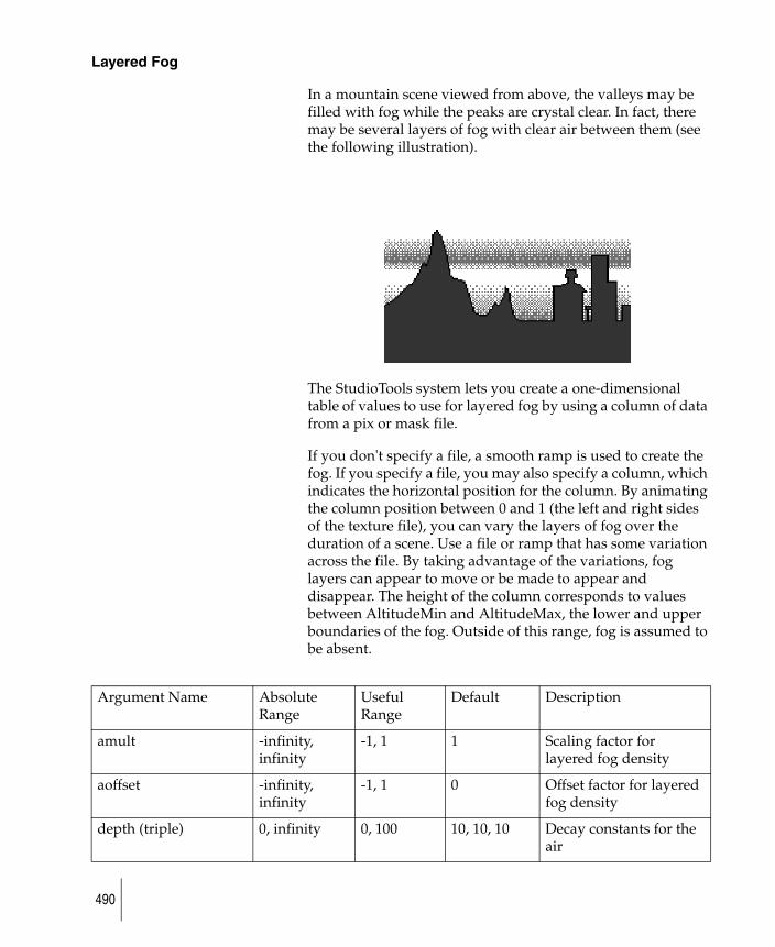
Layered Fog
In a mountain scene viewed from above, the valleys may be filled with fog while the peaks are crystal clear. In fact, there may be several layers of fog with clear air between them (see the following illustration).
The StudioTools system lets you create a one-dimensional table of values to use for layered fog by using a column of data from a pix or mask file.
If you don't specify a file, a smooth ramp is used to create the fog. If you specify a file, you may also specify a column, which indicates the horizontal position for the column. By animating the column position between 0 and 1 (the left and right sides of the texture file), you can vary the layers of fog over the duration of a scene. Use a file or ramp that has some variation across the file. By taking advantage of the variations, fog layers can appear to move or be made to appear and disappear. The height of the column corresponds to values between AltitudeMin and AltitudeMax, the lower and upper boundaries of the fog. Outside of this range, fog is assumed to be absent.
Argument Name Absolute Range
Useful Range
Default Description
amult -infinity, infinity
-1, 1 1 Scaling factor for layered fog density
aoffset -infinity, infinity
-1, 1 0 Offset factor for layered fog density
depth (triple) 0, infinity 0, 100 10, 10, 10 Decay constants for the air
490
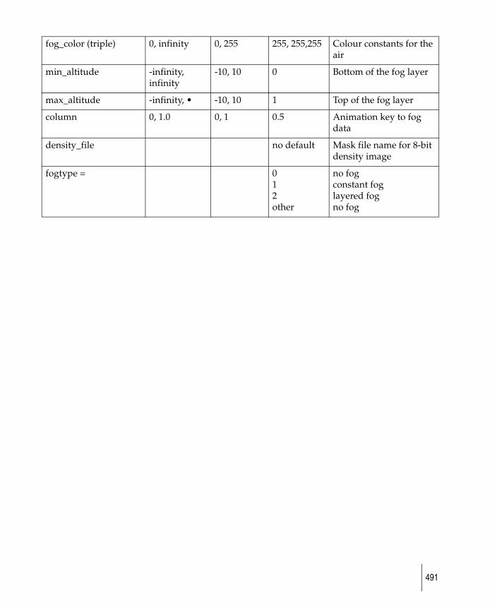
fog_color (triple) 0, infinity 0, 255 255, 255,255 Colour constants for the air
min_altitude -infinity, infinity
-10, 10 0 Bottom of the fog layer
max_altitude -infinity, • -10, 10 1 Top of the fog layer
column 0, 1.0 0, 1 0.5 Animation key to fog data
density_file no default Mask file name for 8-bit density image
fogtype = 012other
no fogconstant foglayered fogno fog
491

Bulge
The Bulge texture procedure was inspired by looking at windows on a skyscraper. If a building was pumped full of air, the glass would bulge outwards in the center while the edges would be constrained by the frame. The frame of the window is exactly the same as a grid that is apparent when using the bulge texture.
The Bulge texture procedure is most commonly applied as a bump map to create a bulge effect on a surface. However, it can also be applied to a transparency map to simulate windows that are dirty or opaque around the edges but transparent in the middle area. When applied to a color map, there is no apparent bulge, but this application can be used to simulate tile effects, for example.
Argument Name
Absolute Range
Useful Range Default Description
uwidth 0.0, 1.0 0, 1 0.1 Width in u dir. of constant stripe
vwidth 0.0, 1.0 0, 1 0.1 Width in v dir. of constant stripe
urepeat -infinity, infinity
-10.0, 10.0 1.0 # of copies in u dir. within coverage area.
vrepeat -infinity, infinity
-10.0, 10.0 1.0 # of copies in v dir. within coverage area.
uoffset -infinity, infinity
-1.0, 1.0 0.0 U offset repeat within coverage area
voffset -infinity, infinity
-1.0, 1.0 0.0 V offset repeat within coverage area
ucoverage -infinity, infinity
0.0, 1.0 1.0 amount of U surface to be textured
vcoverage -infinity, infinity
0.0, 1.0 1.0 amount of V surface to be textured
utranslate -infinity, infinity
-1.0, 1.0 0.0 amount of U coverage area to be moved.
vtranslate -infinity, infinity
-1.0, 1.0 0.0 amount of V coverage area to be moved.
492
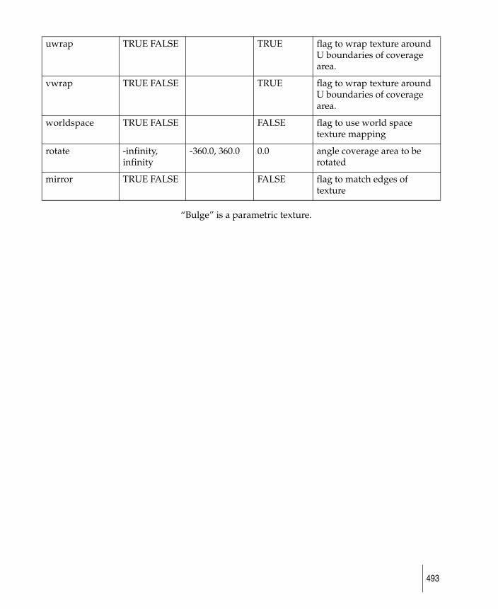
“Bulge” is a parametric texture.
uwrap TRUE FALSE TRUE flag to wrap texture around U boundaries of coverage area.
vwrap TRUE FALSE TRUE flag to wrap texture around U boundaries of coverage area.
worldspace TRUE FALSE FALSE flag to use world space texture mapping
rotate -infinity, infinity
-360.0, 360.0 0.0 angle coverage area to be rotated
mirror TRUE FALSE FALSE flag to match edges of texture
493
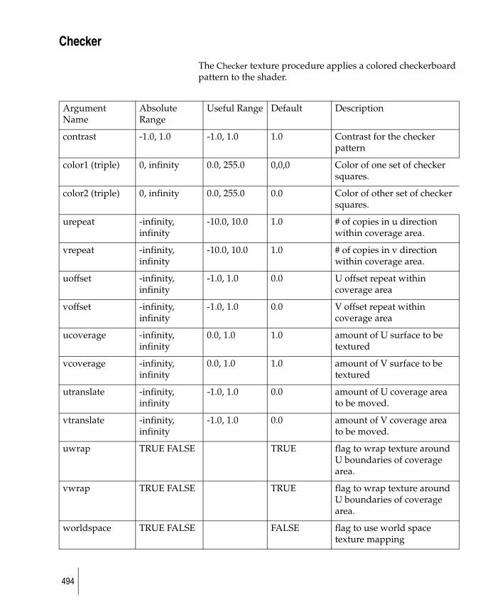
Checker
The Checker texture procedure applies a colored checkerboard pattern to the shader.
Argument Name
Absolute Range
Useful Range Default Description
contrast -1.0, 1.0 -1.0, 1.0 1.0 Contrast for the checker pattern
color1 (triple) 0, infinity 0.0, 255.0 0,0,0 Color of one set of checker squares.
color2 (triple) 0, infinity 0.0, 255.0 0.0 Color of other set of checker squares.
urepeat -infinity, infinity
-10.0, 10.0 1.0 # of copies in u direction within coverage area.
vrepeat -infinity, infinity
-10.0, 10.0 1.0 # of copies in v direction within coverage area.
uoffset -infinity, infinity
-1.0, 1.0 0.0 U offset repeat within coverage area
voffset -infinity, infinity
-1.0, 1.0 0.0 V offset repeat within coverage area
ucoverage -infinity, infinity
0.0, 1.0 1.0 amount of U surface to be textured
vcoverage -infinity, infinity
0.0, 1.0 1.0 amount of V surface to be textured
utranslate -infinity, infinity
-1.0, 1.0 0.0 amount of U coverage area to be moved.
vtranslate -infinity, infinity
-1.0, 1.0 0.0 amount of V coverage area to be moved.
uwrap TRUE FALSE TRUE flag to wrap texture around U boundaries of coverage area.
vwrap TRUE FALSE TRUE flag to wrap texture around U boundaries of coverage area.
worldspace TRUE FALSE FALSE flag to use world space texture mapping
494

“Checker” is a parametric texture.
rotate -infinity, infinity
-360.0, 360.0 0.0 angle coverage area to be rotated
mirror TRUE FALSE FALSE flag to match edges of texture
495

Cloth texture
The Cloth texture procedure is ideal for creating fabric-like textures and a variety of other woven effects. In addition to being used as a simple two-dimensional texture, the Cloth procedure is also effective with bump mapping.
For very fine weaves, aliasing may be a problem, particularly when the cloth is viewed from a distance. In this case, the cloth can be turned into a pix file image by using the cloth texture as a Background Environment rather than applying it to a shader. Once the background has been rendered, the resulting pix file can then be applied to the shader as a file texture.
When applied to a bump map, the cloth texture generally produces better effects when both thread colors are white and the gap color is black. The Color Balance options are replaced by the Intensity options, Amult and Aoffset. These options enable you to control the degree of the bump effect. Decreasing the Blurmult value provides greater definition in the bump effect. Generally, both the Amult and Blurmult values should be quite low, that is less than 0.1.
Argument Name Absolute Range
Useful Range
Default Description
u_thread_color -infinity, infinity
0, 255 255.0, 255.0, 255.0 RGB value assigned to warp of fabric
v_thread_color -infinity, infinity
0, 255 255.0, 0.0, 0.0 RGB value assigned to weft of fabric
gap_color -infinity, infinity
0, 255 0.0, 0.0, 0.0 RGB value assigned to area between threads
u_thread_width 0, 1 0, 1 0.75 Width of warp threads
v_thread_width 0, 1 0, 1 0.75 Width of weft threads
u_wave -infinity, infinity
-0.5, 0.5 0.0 Wave pattern of warp
496
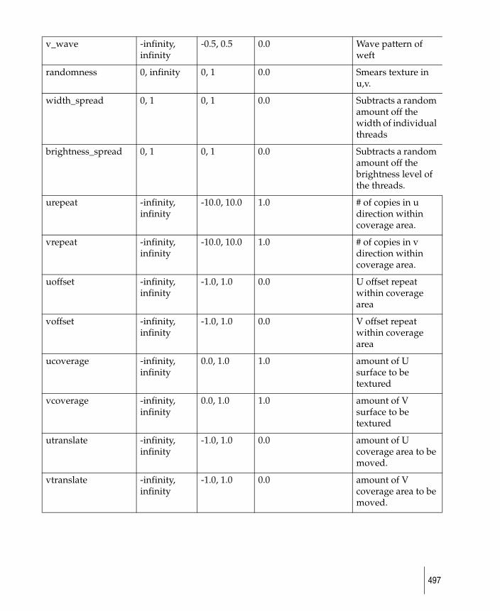
v_wave -infinity, infinity
-0.5, 0.5 0.0 Wave pattern of weft
randomness 0, infinity 0, 1 0.0 Smears texture in u,v.
width_spread 0, 1 0, 1 0.0 Subtracts a random amount off the width of individual threads
brightness_spread 0, 1 0, 1 0.0 Subtracts a random amount off the brightness level of the threads.
urepeat -infinity, infinity
-10.0, 10.0 1.0 # of copies in u direction within coverage area.
vrepeat -infinity, infinity
-10.0, 10.0 1.0 # of copies in v direction within coverage area.
uoffset -infinity, infinity
-1.0, 1.0 0.0 U offset repeat within coverage area
voffset -infinity, infinity
-1.0, 1.0 0.0 V offset repeat within coverage area
ucoverage -infinity, infinity
0.0, 1.0 1.0 amount of U surface to be textured
vcoverage -infinity, infinity
0.0, 1.0 1.0 amount of V surface to be textured
utranslate -infinity, infinity
-1.0, 1.0 0.0 amount of U coverage area to be moved.
vtranslate -infinity, infinity
-1.0, 1.0 0.0 amount of V coverage area to be moved.
497
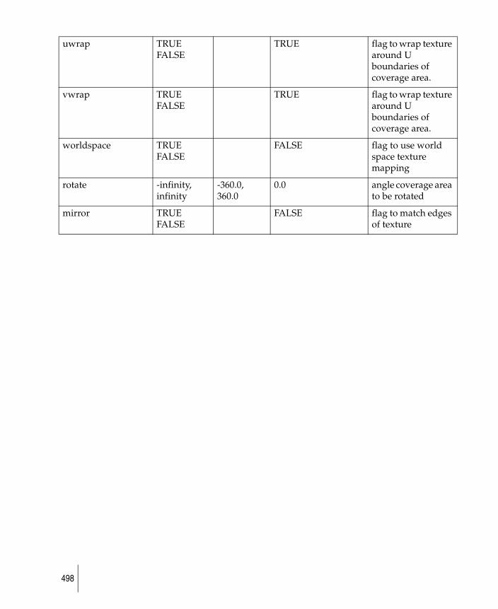
uwrap TRUE FALSE
TRUE flag to wrap texture around U boundaries of coverage area.
vwrap TRUE FALSE
TRUE flag to wrap texture around U boundaries of coverage area.
worldspace TRUE FALSE
FALSE flag to use world space texture mapping
rotate -infinity, infinity
-360.0, 360.0
0.0 angle coverage area to be rotated
mirror TRUE FALSE
FALSE flag to match edges of texture
498
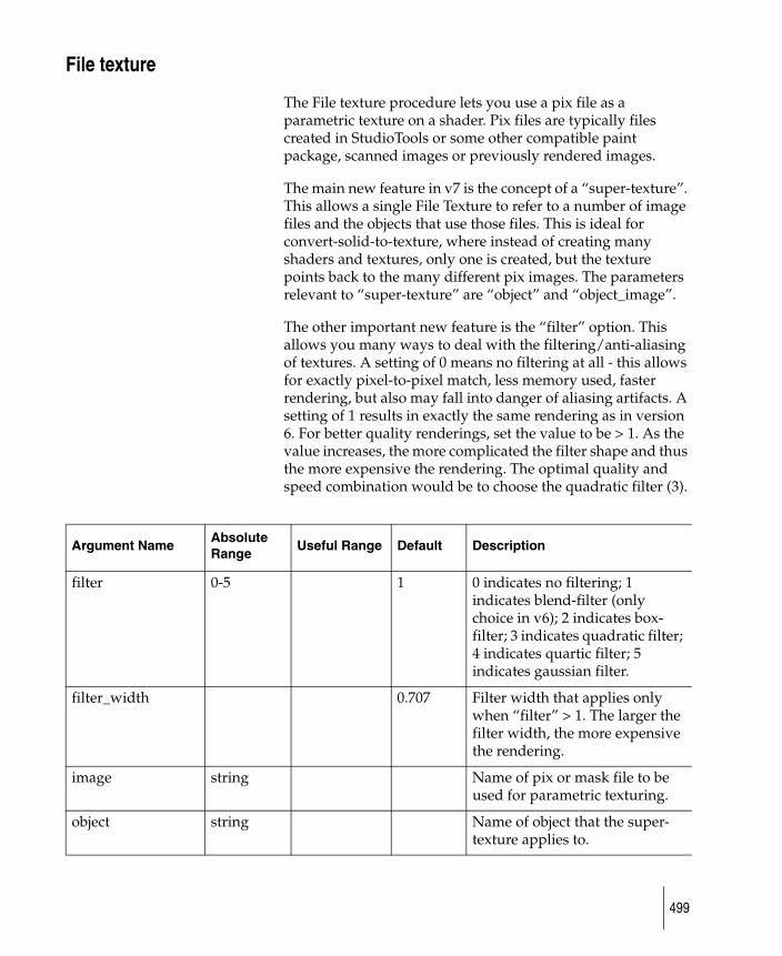
File texture
The File texture procedure lets you use a pix file as a parametric texture on a shader. Pix files are typically files created in StudioTools or some other compatible paint package, scanned images or previously rendered images.
The main new feature in v7 is the concept of a “super-texture”. This allows a single File Texture to refer to a number of image files and the objects that use those files. This is ideal for convert-solid-to-texture, where instead of creating many shaders and textures, only one is created, but the texture points back to the many different pix images. The parameters relevant to “super-texture” are “object” and “object_image”.
The other important new feature is the “filter” option. This allows you many ways to deal with the filtering/anti-aliasing of textures. A setting of 0 means no filtering at all - this allows for exactly pixel-to-pixel match, less memory used, faster rendering, but also may fall into danger of aliasing artifacts. A setting of 1 results in exactly the same rendering as in version 6. For better quality renderings, set the value to be > 1. As the value increases, the more complicated the filter shape and thus the more expensive the rendering. The optimal quality and speed combination would be to choose the quadratic filter (3).
Argument NameAbsolute Range
Useful Range Default Description
filter 0-5 1 0 indicates no filtering; 1 indicates blend-filter (only choice in v6); 2 indicates box-filter; 3 indicates quadratic filter; 4 indicates quartic filter; 5 indicates gaussian filter.
filter_width 0.707 Filter width that applies only when “filter” > 1. The larger the filter width, the more expensive the rendering.
image string Name of pix or mask file to be used for parametric texturing.
object string Name of object that the super-texture applies to.
499
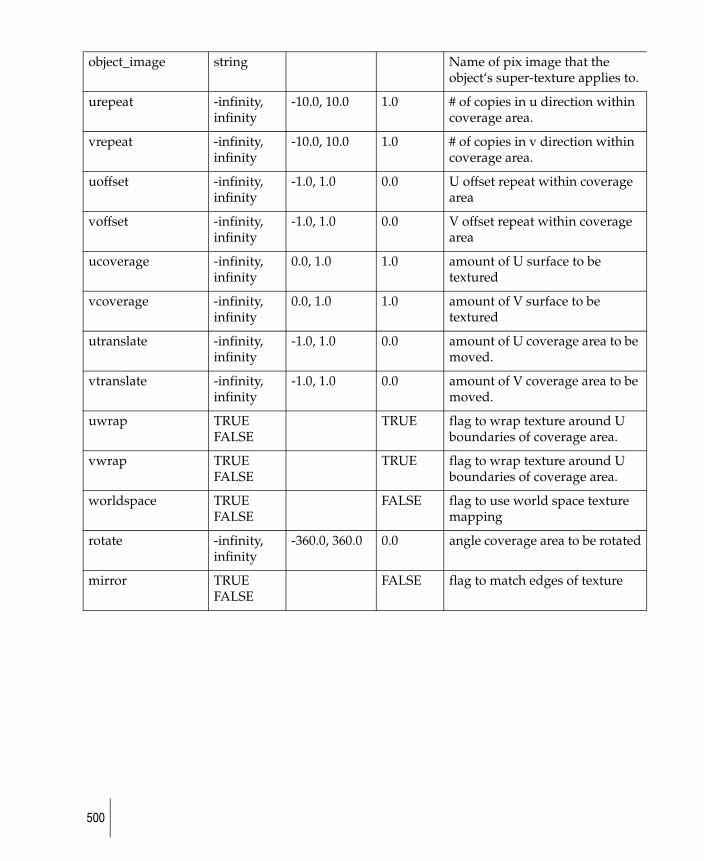
object_image string Name of pix image that the object‘s super-texture applies to.
urepeat -infinity, infinity
-10.0, 10.0 1.0 # of copies in u direction within coverage area.
vrepeat -infinity, infinity
-10.0, 10.0 1.0 # of copies in v direction within coverage area.
uoffset -infinity, infinity
-1.0, 1.0 0.0 U offset repeat within coverage area
voffset -infinity, infinity
-1.0, 1.0 0.0 V offset repeat within coverage area
ucoverage -infinity, infinity
0.0, 1.0 1.0 amount of U surface to be textured
vcoverage -infinity, infinity
0.0, 1.0 1.0 amount of V surface to be textured
utranslate -infinity, infinity
-1.0, 1.0 0.0 amount of U coverage area to be moved.
vtranslate -infinity, infinity
-1.0, 1.0 0.0 amount of V coverage area to be moved.
uwrap TRUE FALSE
TRUE flag to wrap texture around U boundaries of coverage area.
vwrap TRUE FALSE
TRUE flag to wrap texture around U boundaries of coverage area.
worldspace TRUE FALSE
FALSE flag to use world space texture mapping
rotate -infinity, infinity
-360.0, 360.0 0.0 angle coverage area to be rotated
mirror TRUE FALSE
FALSE flag to match edges of texture
500
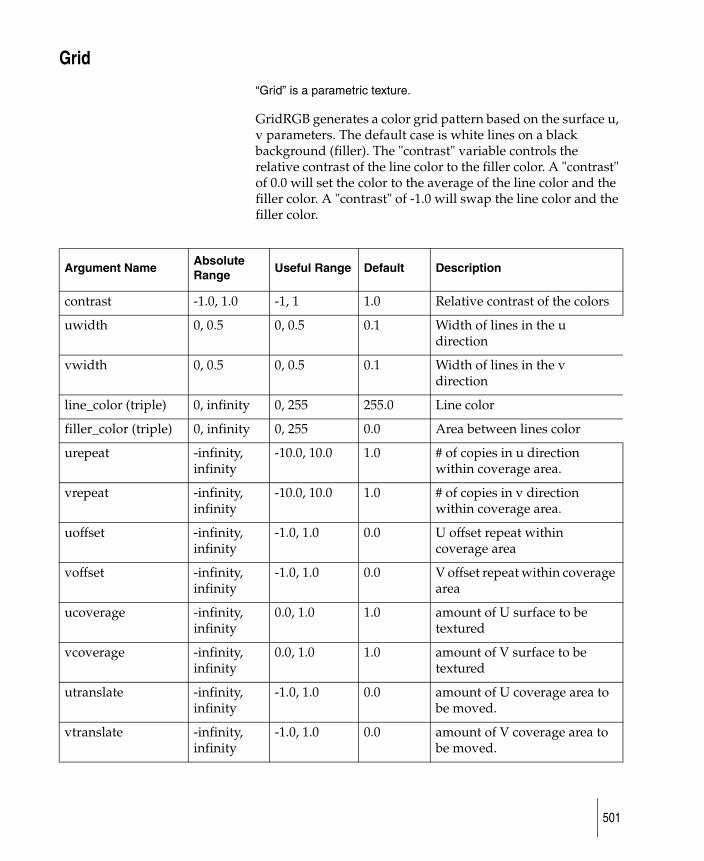
Grid
“Grid” is a parametric texture.
GridRGB generates a color grid pattern based on the surface u, v parameters. The default case is white lines on a black background (filler). The "contrast" variable controls the relative contrast of the line color to the filler color. A "contrast" of 0.0 will set the color to the average of the line color and the filler color. A "contrast" of -1.0 will swap the line color and the filler color.
Argument NameAbsolute Range
Useful Range Default Description
contrast -1.0, 1.0 -1, 1 1.0 Relative contrast of the colors
uwidth 0, 0.5 0, 0.5 0.1 Width of lines in the u direction
vwidth 0, 0.5 0, 0.5 0.1 Width of lines in the v direction
line_color (triple) 0, infinity 0, 255 255.0 Line color
filler_color (triple) 0, infinity 0, 255 0.0 Area between lines color
urepeat -infinity, infinity
-10.0, 10.0 1.0 # of copies in u direction within coverage area.
vrepeat -infinity, infinity
-10.0, 10.0 1.0 # of copies in v direction within coverage area.
uoffset -infinity, infinity
-1.0, 1.0 0.0 U offset repeat within coverage area
voffset -infinity, infinity
-1.0, 1.0 0.0 V offset repeat within coverage area
ucoverage -infinity, infinity
0.0, 1.0 1.0 amount of U surface to be textured
vcoverage -infinity, infinity
0.0, 1.0 1.0 amount of V surface to be textured
utranslate -infinity, infinity
-1.0, 1.0 0.0 amount of U coverage area to be moved.
vtranslate -infinity, infinity
-1.0, 1.0 0.0 amount of V coverage area to be moved.
501
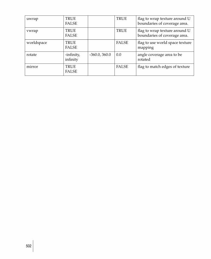
uwrap TRUE FALSE
TRUE flag to wrap texture around U boundaries of coverage area.
vwrap TRUE FALSE
TRUE flag to wrap texture around U boundaries of coverage area.
worldspace TRUE FALSE
FALSE flag to use world space texture mapping
rotate -infinity, infinity
-360.0, 360.0 0.0 angle coverage area to be rotated
mirror TRUE FALSE
FALSE flag to match edges of texture
502
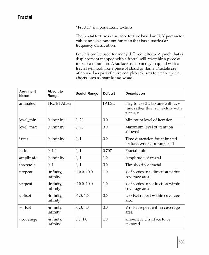
Fractal
“Fractal” is a parametric texture.
The Fractal texture is a surface texture based on U, V parameter values and is a random function that has a particular frequency distribution.
Fractals can be used for many different effects. A patch that is displacement mapped with a fractal will resemble a piece of rock or a mountain. A surface transparency mapped with a fractal will look like a piece of cloud or flame. Fractals are often used as part of more complex textures to create special effects such as marble and wood.
Argument Name
Absolute Range
Useful Range Default Description
animated TRUE FALSE FALSE Flag to use 3D texture with u, v, time rather than 2D texture with just u, v
level_min 0, infinity 0, 20 0.0 Minimum level of iteration
level_max 0, infinity 0, 20 9.0 Maximum level of iteration allowed
*time 0, infinity 0, 1 0.0 Time dimension for animated texture, wraps for range 0, 1
ratio 0, 1.0 0, 1 0.707 Fractal ratio
amplitude 0, infinity 0, 1 1.0 Amplitude of fractal
threshold 0, 1 0, 1 0.0 Threshold for fractal
urepeat -infinity, infinity
-10.0, 10.0 1.0 # of copies in u direction within coverage area.
vrepeat -infinity, infinity
-10.0, 10.0 1.0 # of copies in v direction within coverage area.
uoffset -infinity, infinity
-1.0, 1.0 0.0 U offset repeat within coverage area
voffset -infinity, infinity
-1.0, 1.0 0.0 V offset repeat within coverage area
ucoverage -infinity, infinity
0.0, 1.0 1.0 amount of U surface to be textured
503
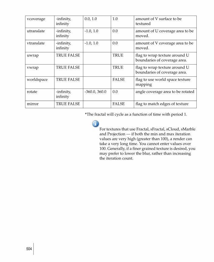
*The fractal will cycle as a function of time with period 1.
For textures that use Fractal, sFractal, sCloud, sMarble and Projection — if both the min and max iteration values are very high (greater than 100), a render can take a very long time. You cannot enter values over 100. Generally, if a finer grained texture is desired, you may prefer to lower the blur, rather than increasing the iteration count.
vcoverage -infinity, infinity
0.0, 1.0 1.0 amount of V surface to be textured
utranslate -infinity, infinity
-1.0, 1.0 0.0 amount of U coverage area to be moved.
vtranslate -infinity, infinity
-1.0, 1.0 0.0 amount of V coverage area to be moved.
uwrap TRUE FALSE TRUE flag to wrap texture around U boundaries of coverage area.
vwrap TRUE FALSE TRUE flag to wrap texture around U boundaries of coverage area.
worldspace TRUE FALSE FALSE flag to use world space texture mapping
rotate -infinity, infinity
-360.0, 360.0 0.0 angle coverage area to be rotated
mirror TRUE FALSE FALSE flag to match edges of texture
504
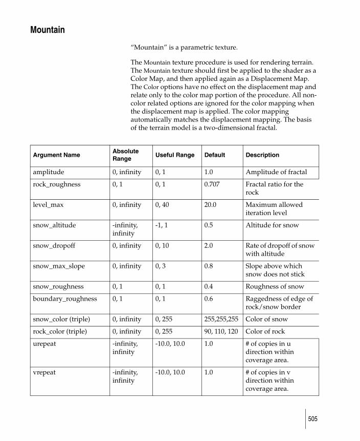
Mountain
“Mountain” is a parametric texture.
The Mountain texture procedure is used for rendering terrain. The Mountain texture should first be applied to the shader as a Color Map, and then applied again as a Displacement Map. The Color options have no effect on the displacement map and relate only to the color map portion of the procedure. All non-color related options are ignored for the color mapping when the displacement map is applied. The color mapping automatically matches the displacement mapping. The basis of the terrain model is a two-dimensional fractal.
Argument NameAbsolute Range
Useful Range Default Description
amplitude 0, infinity 0, 1 1.0 Amplitude of fractal
rock_roughness 0, 1 0, 1 0.707 Fractal ratio for the rock
level_max 0, infinity 0, 40 20.0 Maximum allowed iteration level
snow_altitude -infinity, infinity
-1, 1 0.5 Altitude for snow
snow_dropoff 0, infinity 0, 10 2.0 Rate of dropoff of snow with altitude
snow_max_slope 0, infinity 0, 3 0.8 Slope above which snow does not stick
snow_roughness 0, 1 0, 1 0.4 Roughness of snow
boundary_roughness 0, 1 0, 1 0.6 Raggedness of edge of rock/snow border
snow_color (triple) 0, infinity 0, 255 255,255,255 Color of snow
rock_color (triple) 0, infinity 0, 255 90, 110, 120 Color of rock
urepeat -infinity, infinity
-10.0, 10.0 1.0 # of copies in u direction within coverage area.
vrepeat -infinity, infinity
-10.0, 10.0 1.0 # of copies in v direction within coverage area.
505
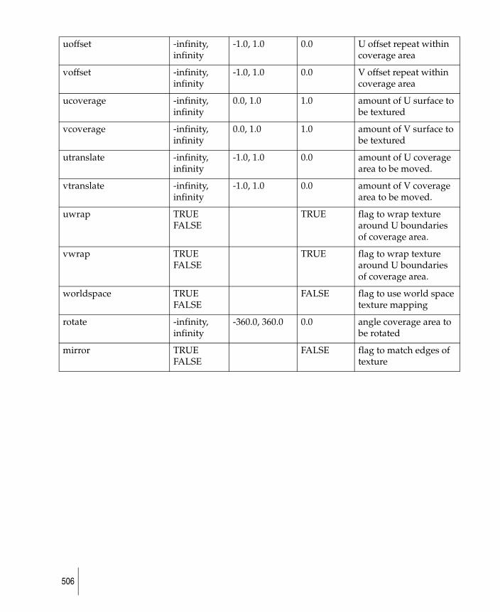
uoffset -infinity, infinity
-1.0, 1.0 0.0 U offset repeat within coverage area
voffset -infinity, infinity
-1.0, 1.0 0.0 V offset repeat within coverage area
ucoverage -infinity, infinity
0.0, 1.0 1.0 amount of U surface to be textured
vcoverage -infinity, infinity
0.0, 1.0 1.0 amount of V surface to be textured
utranslate -infinity, infinity
-1.0, 1.0 0.0 amount of U coverage area to be moved.
vtranslate -infinity, infinity
-1.0, 1.0 0.0 amount of V coverage area to be moved.
uwrap TRUE FALSE
TRUE flag to wrap texture around U boundaries of coverage area.
vwrap TRUE FALSE
TRUE flag to wrap texture around U boundaries of coverage area.
worldspace TRUE FALSE
FALSE flag to use world space texture mapping
rotate -infinity, infinity
-360.0, 360.0 0.0 angle coverage area to be rotated
mirror TRUE FALSE
FALSE flag to match edges of texture
506
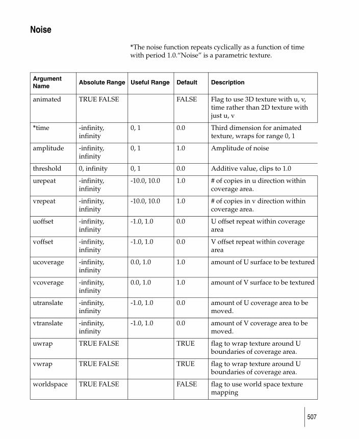
Noise
*The noise function repeats cyclically as a function of time with period 1.0.“Noise” is a parametric texture.
Argument Name
Absolute Range Useful Range Default Description
animated TRUE FALSE FALSE Flag to use 3D texture with u, v, time rather than 2D texture with just u, v
*time -infinity, infinity
0, 1 0.0 Third dimension for animated texture, wraps for range 0, 1
amplitude -infinity, infinity
0, 1 1.0 Amplitude of noise
threshold 0, infinity 0, 1 0.0 Additive value, clips to 1.0
urepeat -infinity, infinity
-10.0, 10.0 1.0 # of copies in u direction within coverage area.
vrepeat -infinity, infinity
-10.0, 10.0 1.0 # of copies in v direction within coverage area.
uoffset -infinity, infinity
-1.0, 1.0 0.0 U offset repeat within coverage area
voffset -infinity, infinity
-1.0, 1.0 0.0 V offset repeat within coverage area
ucoverage -infinity, infinity
0.0, 1.0 1.0 amount of U surface to be textured
vcoverage -infinity, infinity
0.0, 1.0 1.0 amount of V surface to be textured
utranslate -infinity, infinity
-1.0, 1.0 0.0 amount of U coverage area to be moved.
vtranslate -infinity, infinity
-1.0, 1.0 0.0 amount of V coverage area to be moved.
uwrap TRUE FALSE TRUE flag to wrap texture around U boundaries of coverage area.
vwrap TRUE FALSE TRUE flag to wrap texture around U boundaries of coverage area.
worldspace TRUE FALSE FALSE flag to use world space texture mapping
507
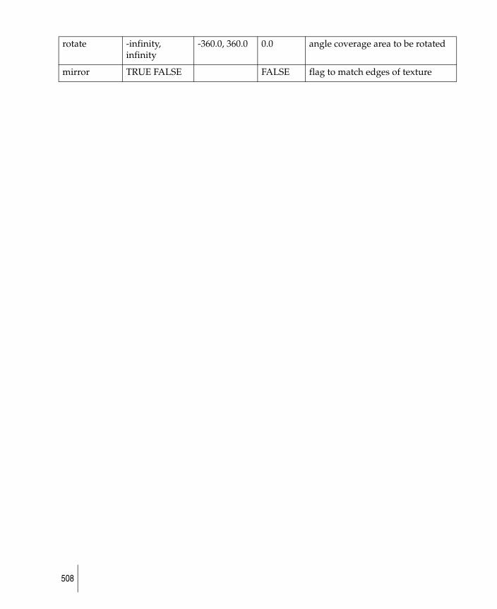
rotate -infinity, infinity
-360.0, 360.0 0.0 angle coverage area to be rotated
mirror TRUE FALSE FALSE flag to match edges of texture
508
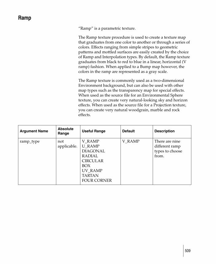
Ramp
“Ramp” is a parametric texture.
The Ramp texture procedure is used to create a texture map that graduates from one color to another or through a series of colors. Effects ranging from simple stripes to geometric patterns and mottled surfaces are easily created by the choice of Ramp and Interpolation types. By default, the Ramp texture graduates from black to red to blue in a linear, horizontal (V ramp) fashion. When applied to a Bump map however, the colors in the ramp are represented as a gray scale.
The Ramp texture is commonly used as a two-dimensional Environment background, but can also be used with other map types such as the transparency map for special effects. When used as the source file for an Environmental Sphere texture, you can create very natural-looking sky and horizon effects. When used as the source file for a Projection texture, you can create very natural woodgrain, marble and rock effects.
Argument NameAbsolute Range
Useful Range Default Description
ramp_type not applicable.
V_RAMPU_RAMPDIAGONALRADIALCIRCULARBOXUV_RAMPTARTANFOUR CORNER
V_RAMP There are nine different ramp types to choose from.
509
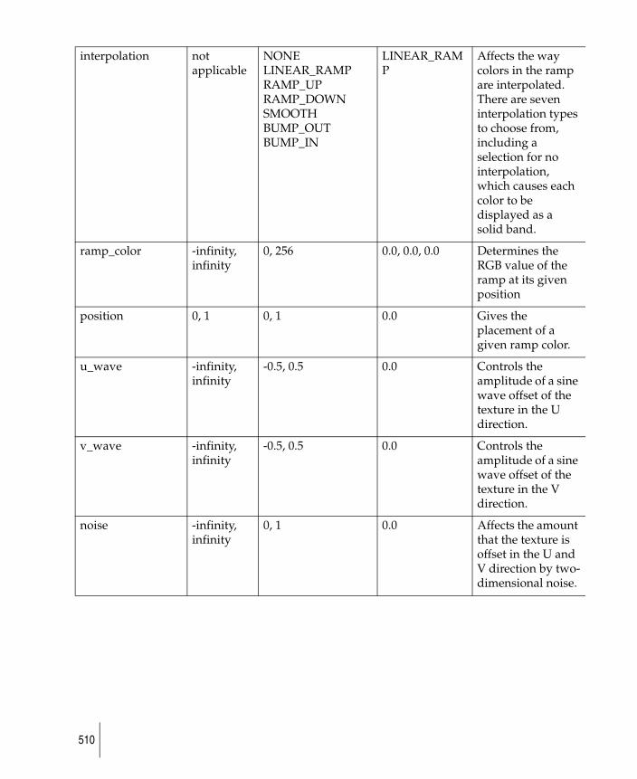
interpolation not applicable
NONELINEAR_RAMPRAMP_UPRAMP_DOWNSMOOTHBUMP_OUTBUMP_IN
LINEAR_RAMP
Affects the way colors in the ramp are interpolated. There are seven interpolation types to choose from, including a selection for no interpolation, which causes each color to be displayed as a solid band.
ramp_color -infinity, infinity
0, 256 0.0, 0.0, 0.0 Determines the RGB value of the ramp at its given position
position 0, 1 0, 1 0.0 Gives the placement of a given ramp color.
u_wave -infinity, infinity
-0.5, 0.5 0.0 Controls the amplitude of a sine wave offset of the texture in the U direction.
v_wave -infinity, infinity
-0.5, 0.5 0.0 Controls the amplitude of a sine wave offset of the texture in the V direction.
noise -infinity, infinity
0, 1 0.0 Affects the amount that the texture is offset in the U and V direction by two-dimensional noise.
510
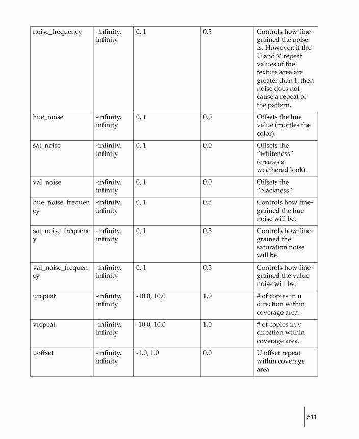
noise_frequency -infinity, infinity
0, 1 0.5 Controls how fine-grained the noise is. However, if the U and V repeat values of the texture area are greater than 1, then noise does not cause a repeat of the pattern.
hue_noise -infinity, infinity
0, 1 0.0 Offsets the hue value (mottles the color).
sat_noise -infinity, infinity
0, 1 0.0 Offsets the “whiteness” (creates a weathered look).
val_noise -infinity, infinity
0, 1 0.0 Offsets the “blackness.”
hue_noise_frequency
-infinity, infinity
0, 1 0.5 Controls how fine-grained the hue noise will be.
sat_noise_frequency
-infinity, infinity
0, 1 0.5 Controls how fine-grained the saturation noise will be.
val_noise_frequency
-infinity, infinity
0, 1 0.5 Controls how fine-grained the value noise will be.
urepeat -infinity, infinity
-10.0, 10.0 1.0 # of copies in u direction within coverage area.
vrepeat -infinity, infinity
-10.0, 10.0 1.0 # of copies in v direction within coverage area.
uoffset -infinity, infinity
-1.0, 1.0 0.0 U offset repeat within coverage area
511
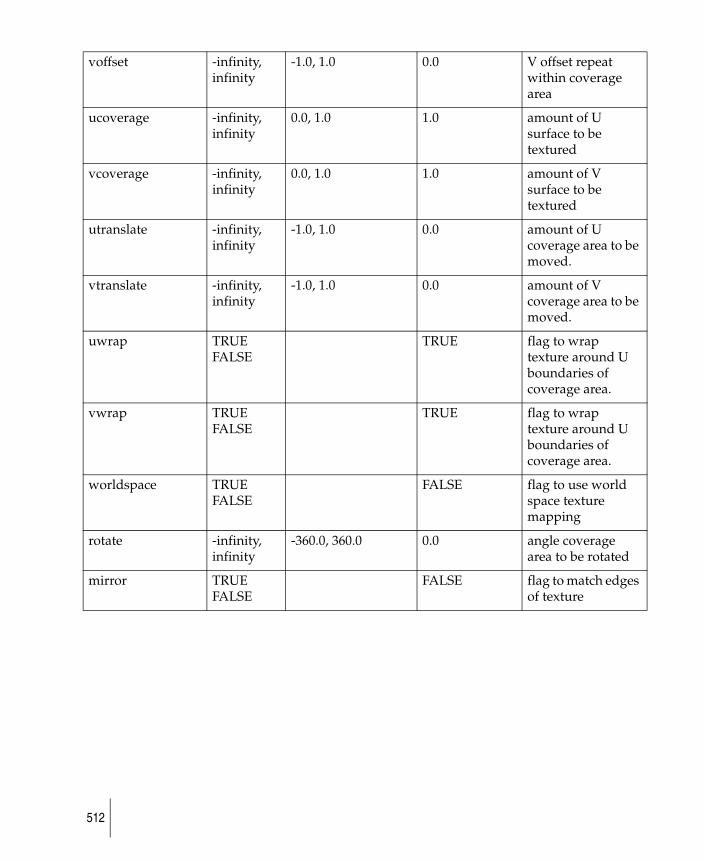
voffset -infinity, infinity
-1.0, 1.0 0.0 V offset repeat within coverage area
ucoverage -infinity, infinity
0.0, 1.0 1.0 amount of U surface to be textured
vcoverage -infinity, infinity
0.0, 1.0 1.0 amount of V surface to be textured
utranslate -infinity, infinity
-1.0, 1.0 0.0 amount of U coverage area to be moved.
vtranslate -infinity, infinity
-1.0, 1.0 0.0 amount of V coverage area to be moved.
uwrap TRUE FALSE
TRUE flag to wrap texture around U boundaries of coverage area.
vwrap TRUE FALSE
TRUE flag to wrap texture around U boundaries of coverage area.
worldspace TRUE FALSE
FALSE flag to use world space texture mapping
rotate -infinity, infinity
-360.0, 360.0 0.0 angle coverage area to be rotated
mirror TRUE FALSE
FALSE flag to match edges of texture
512

Stencil
“Stencil” is a parametric texture.
The Stencil texture procedure is used mainly for label mapping purposes. Label mapping is a two-dimensional texture that is usually applied as a Color map onto a surface and often includes a transparency component to mask certain parts of the two-dimensional texture. An example of label mapping is consumer packaging items such as a shampoo bottle with a label. The labels often hold opaque colors combined with transparent areas. The Stencil texture procedure enables you to easily place the two-dimensional label map and create the necessary transparency mask.
Argument NameAbsolute Range
Useful Range
Default Description
image_file (string) name of the pix file to be used as a label map
edge_blend 0, infinity 0, 1 0.0 Softens the edges of the texture coverage area. This is useful for hiding the texture boundary when the mask is not perfect.
mask_file (string) name of the mask file to be used as a label map
mask_level -infinity, infinity
-1, 1 1.0 Varies the degree of transparency of the color areas. At a value of 1 (the default), all white areas of the mask are totally transparent and all black areas are totally opaque. As you decrease the value towards 0.00, the black areas become more transparent. By the time you reach 0.00, no image transparency masking occurs. If you decrease the mask_level to -1.00, the mask is inverted, where the black areas become transparent and the white areas are opaque.
mask_blur 0, infinity 0, 0.25 0.0 Affects the edges of the mask. At a value of 0.00, there is no mask blurring. As you increase the blur value, the edges of the mask are blurred to produce soft edge transparency effects.
513
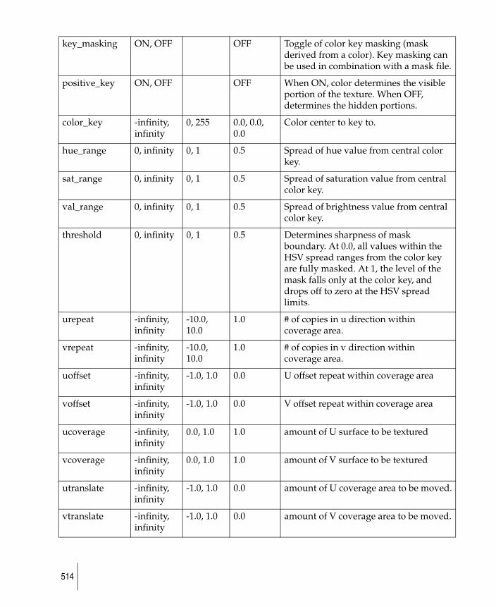
key_masking ON, OFF OFF Toggle of color key masking (mask derived from a color). Key masking can be used in combination with a mask file.
positive_key ON, OFF OFF When ON, color determines the visible portion of the texture. When OFF, determines the hidden portions.
color_key -infinity, infinity
0, 255 0.0, 0.0, 0.0
Color center to key to.
hue_range 0, infinity 0, 1 0.5 Spread of hue value from central color key.
sat_range 0, infinity 0, 1 0.5 Spread of saturation value from central color key.
val_range 0, infinity 0, 1 0.5 Spread of brightness value from central color key.
threshold 0, infinity 0, 1 0.5 Determines sharpness of mask boundary. At 0.0, all values within the HSV spread ranges from the color key are fully masked. At 1, the level of the mask falls only at the color key, and drops off to zero at the HSV spread limits.
urepeat -infinity, infinity
-10.0, 10.0
1.0 # of copies in u direction within coverage area.
vrepeat -infinity, infinity
-10.0, 10.0
1.0 # of copies in v direction within coverage area.
uoffset -infinity, infinity
-1.0, 1.0 0.0 U offset repeat within coverage area
voffset -infinity, infinity
-1.0, 1.0 0.0 V offset repeat within coverage area
ucoverage -infinity, infinity
0.0, 1.0 1.0 amount of U surface to be textured
vcoverage -infinity, infinity
0.0, 1.0 1.0 amount of V surface to be textured
utranslate -infinity, infinity
-1.0, 1.0 0.0 amount of U coverage area to be moved.
vtranslate -infinity, infinity
-1.0, 1.0 0.0 amount of V coverage area to be moved.
514
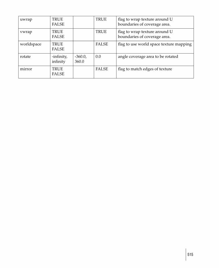
uwrap TRUE FALSE
TRUE flag to wrap texture around U boundaries of coverage area.
vwrap TRUE FALSE
TRUE flag to wrap texture around U boundaries of coverage area.
worldspace TRUE FALSE
FALSE flag to use world space texture mapping
rotate -infinity, infinity
-360.0, 360.0
0.0 angle coverage area to be rotated
mirror TRUE FALSE
FALSE flag to match edges of texture
515
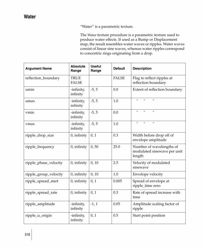
Water
“Water” is a parametric texture.
The Water texture procedure is a parametric texture used to produce water effects. If used as a Bump or Displacement map, the result resembles water waves or ripples. Water waves consist of linear sine waves, whereas water ripples correspond to concentric rings originating from a drop.
Argument NameAbsolute Range
Useful Range
Default Description
reflection_boundary TRUE FALSE
FALSE Flag to reflect ripples at reflection boundary
umin -infinity, infinity
-5, 5 0.0 Extent of reflection boundary
umax -infinity, infinity
-5, 5 1.0 " " "
vmin -infinity, infinity
-5, 5 0.0 " " "
vmax -infinity, infinity
-5, 5 1.0 " " "
ripple_drop_size 0, infinity 0, 1 0.3 Width before drop off of envelope amplitude
ripple_frequency 0, infinity 0, 50 25.0 Number of wavelengths of modulated sinewave per unit length
ripple_phase_velocity 0, infinity 0, 10 2.5 Velocity of modulated sinewave
ripple_group_velocity 0, infinity 0, 10 1.0 Envelope velocity
ripple_spread_start 0, infinity 0, 1 0.005 Spread of envelope at ripple_time zero
ripple_spread_rate 0, infinity 0, 1 0.3 Rate of spread increase with time
ripple_amplitude -infinity, infinity
-1, 1 0.05 Amplitude scaling factor of ripple
ripple_u_origin -infinity, infinity
0, 1 0.5 Start point position
516
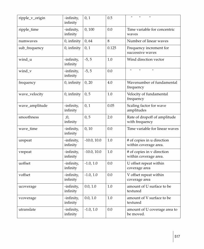
ripple_v_origin -infinity, infinity
0, 1 0.5 " " "
ripple_time -infinity, infinity
0, 100 0.0 Time variable for concentric waves
numwaves 0, infinity 0, 64 8 Number of linear waves
sub_frequency 0, infinity 0, 1 0.125 Frequency increment for successive waves
wind_u -infinity, infinity
-5, 5 1.0 Wind direction vector
wind_v -infinity, infinity
-5, 5 0.0 " " "
frequency 0, infinity 0, 20 4.0 Wavenumber of fundamental frequency
wave_velocity 0, infinity 0, 5 1.0 Velocity of fundamental frequency
wave_amplitude -infinity, infinity
0, 1 0.05 Scaling factor for wave amplitudes
smoothness ;0, infinity
0, 5 2.0 Rate of dropoff of amplitude with frequency
wave_time -infinity, infinity
0, 10 0.0 Time variable for linear waves
urepeat -infinity, infinity
-10.0, 10.0 1.0 # of copies in u direction within coverage area.
vrepeat -infinity, infinity
-10.0, 10.0 1.0 # of copies in v direction within coverage area.
uoffset -infinity, infinity
-1.0, 1.0 0.0 U offset repeat within coverage area
voffset -infinity, infinity
-1.0, 1.0 0.0 V offset repeat within coverage area
ucoverage -infinity, infinity
0.0, 1.0 1.0 amount of U surface to be textured
vcoverage -infinity, infinity
0.0, 1.0 1.0 amount of V surface to be textured
utranslate -infinity, infinity
-1.0, 1.0 0.0 amount of U coverage area to be moved.
517
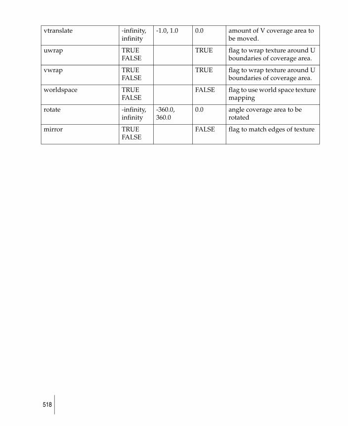
vtranslate -infinity, infinity
-1.0, 1.0 0.0 amount of V coverage area to be moved.
uwrap TRUE FALSE
TRUE flag to wrap texture around U boundaries of coverage area.
vwrap TRUE FALSE
TRUE flag to wrap texture around U boundaries of coverage area.
worldspace TRUE FALSE
FALSE flag to use world space texture mapping
rotate -infinity, infinity
-360.0, 360.0
0.0 angle coverage area to be rotated
mirror TRUE FALSE
FALSE flag to match edges of texture
518
About solid texturesSolid textures use the surface (x, y, z) point to reference into a three dimensional space of texture values. However, the (x, y, z) point is not passed directly to the table. It is first multiplied by a texture transformation matrix. The default case is no specified texture transformation. In that case, the world space surface point is used directly. If an object moves in world space it will move through its solid texture. A wooden object would move through the wood grain. While this may be desirable in certain animations, it is better to have control over solid texture transformations.
If a transformation is to be used, it must be specified using the following syntax.
In the DEFINITION section, the transformation must be declared using
transformation example;
Similarly, the transformation name must be included in the DEFINITION of the texture being used. For example,
color=texture (procedure=Smarble,
transformation_name=example);
In the MODEL section, use
example = current_transformation( );
The assignment statement actually saves the current transformation in the hierarchy. This means that if it is placed immediately before the piece of geometry to be textured, the texture will stick to the geometry independent of the transformation applied to the geometry. It is possible to transform the texture in an arbitrary way by bracketing the assignment statement with its own transformations, e.g.:
{
rotate (xaxis,25);
translate (10,5,2);
example = current_transformation ( );
}
NOTE:
519
1) The definition of the transformation must be BEFORE the definition of the texture.
2) The assignment can be anywhere in the model section, either before or after the patch.
Also note that there is a similar function, current_position, which returns a "triple" - very handy for fancy camera/spotlight motions.
520
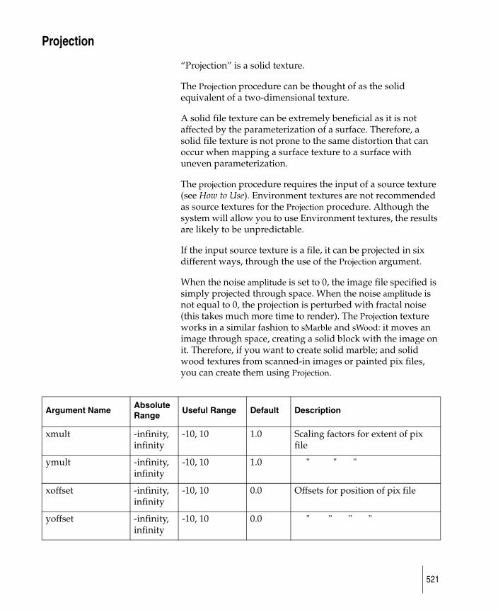
Projection
“Projection” is a solid texture.
The Projection procedure can be thought of as the solid equivalent of a two-dimensional texture.
A solid file texture can be extremely beneficial as it is not affected by the parameterization of a surface. Therefore, a solid file texture is not prone to the same distortion that can occur when mapping a surface texture to a surface with uneven parameterization.
The projection procedure requires the input of a source texture (see How to Use). Environment textures are not recommended as source textures for the Projection procedure. Although the system will allow you to use Environment textures, the results are likely to be unpredictable.
If the input source texture is a file, it can be projected in six different ways, through the use of the Projection argument.
When the noise amplitude is set to 0, the image file specified is simply projected through space. When the noise amplitude is not equal to 0, the projection is perturbed with fractal noise (this takes much more time to render). The Projection texture works in a similar fashion to sMarble and sWood: it moves an image through space, creating a solid block with the image on it. Therefore, if you want to create solid marble; and solid wood textures from scanned-in images or painted pix files, you can create them using Projection.
Argument NameAbsolute Range
Useful Range Default Description
xmult -infinity, infinity
-10, 10 1.0 Scaling factors for extent of pix file
ymult -infinity, infinity
-10, 10 1.0 " " "
xoffset -infinity, infinity
-10, 10 0.0 Offsets for position of pix file
yoffset -infinity, infinity
-10, 10 0.0 " " " "
521
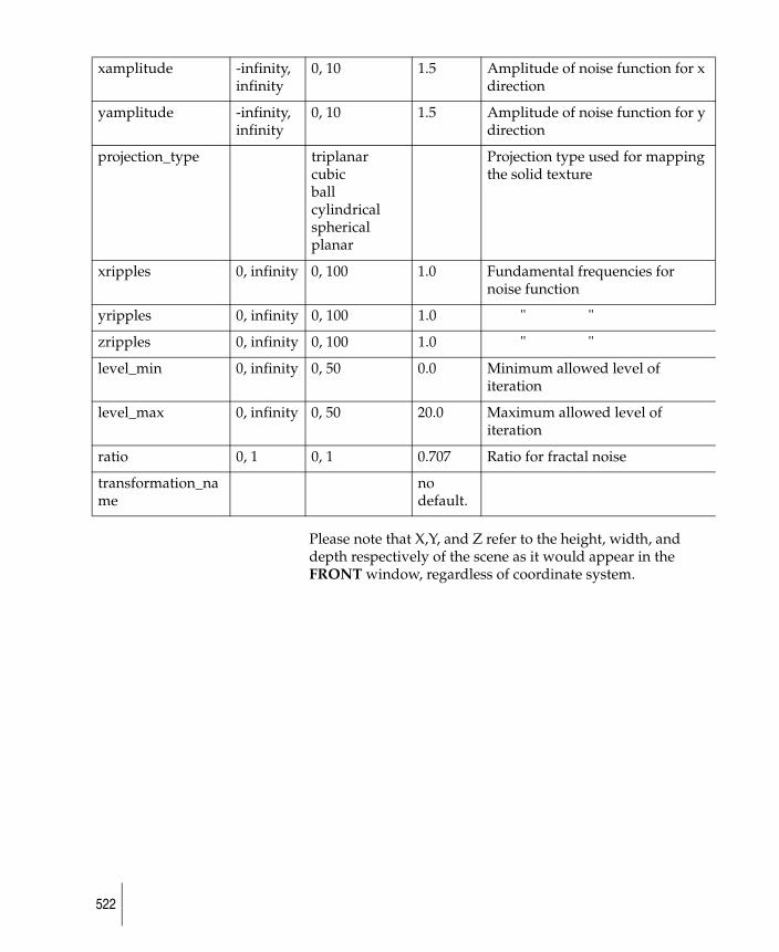
Please note that X,Y, and Z refer to the height, width, and depth respectively of the scene as it would appear in the FRONT window, regardless of coordinate system.
xamplitude -infinity, infinity
0, 10 1.5 Amplitude of noise function for x direction
yamplitude -infinity, infinity
0, 10 1.5 Amplitude of noise function for y direction
projection_type triplanarcubicballcylindricalsphericalplanar
Projection type used for mapping the solid texture
xripples 0, infinity 0, 100 1.0 Fundamental frequencies for noise function
yripples 0, infinity 0, 100 1.0 " "
zripples 0, infinity 0, 100 1.0 " "
level_min 0, infinity 0, 50 0.0 Minimum allowed level of iteration
level_max 0, infinity 0, 50 20.0 Maximum allowed level of iteration
ratio 0, 1 0, 1 0.707 Ratio for fractal noise
transformation_name
no default.
522
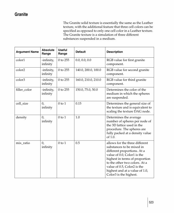
Granite
The Granite solid texture is essentially the same as the Leather texture, with the additional feature that three cell colors can be specified as opposed to only one cell color in a Leather texture. The Granite texture is a simulation of three different substances suspended in a medium.
Argument NameAbsolute Range
Useful Range
Default Description
color1 -infinity, infinity
0 to 255 0.0, 0.0, 0.0 RGB value for first granite component.
color2 -infinity, infinity
0 to 255 140.0, 200.0, 100.0 RGB value for second granite component.
color3 -infinity, infinity
0 to 255 160.0, 210.0, 210.0 RGB value for third granite component.
filler_color -infinity, infinity
0 to 255 150.0, 75.0, 50.0 Determines the color of the medium in which the spheres are suspended.
cell_size 0, infinity
0 to 1 0.15 Determines the general size of the texture and is equivalent to scaling the texture DAG node.
density 0, infinity
0 to 1 1.0 Determines the average number of spheres per node of the 3D lattice used in the procedure. The spheres are fully packed at a density value of 1.0.
mix_ratio 0, infinity
0 to 1 0.5 allows for the three different substances to be mixed in different proportions. At a value of 0.0, Color1 is the highest in terms of proportion to the other two colors. At a value of 0.5, Color2 is the highest and at a value of 1.0, Color3 is the highest.
523
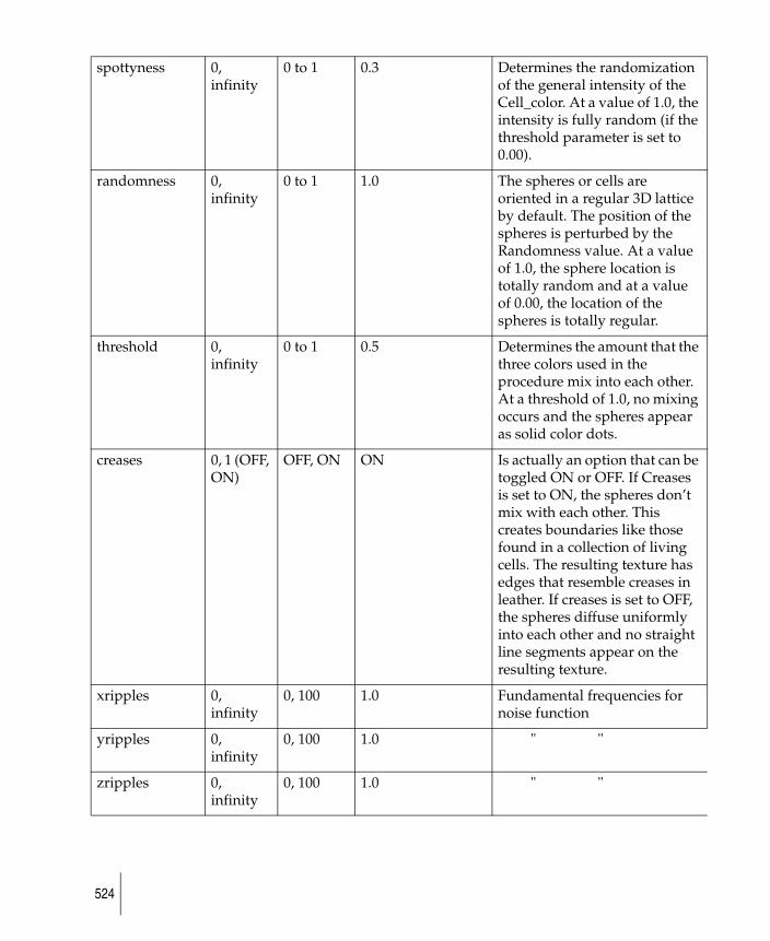
spottyness 0, infinity
0 to 1 0.3 Determines the randomization of the general intensity of the Cell_color. At a value of 1.0, the intensity is fully random (if the threshold parameter is set to 0.00).
randomness 0, infinity
0 to 1 1.0 The spheres or cells are oriented in a regular 3D lattice by default. The position of the spheres is perturbed by the Randomness value. At a value of 1.0, the sphere location is totally random and at a value of 0.00, the location of the spheres is totally regular.
threshold 0, infinity
0 to 1 0.5 Determines the amount that the three colors used in the procedure mix into each other. At a threshold of 1.0, no mixing occurs and the spheres appear as solid color dots.
creases 0, 1 (OFF, ON)
OFF, ON ON Is actually an option that can be toggled ON or OFF. If Creases is set to ON, the spheres don’t mix with each other. This creates boundaries like those found in a collection of living cells. The resulting texture has edges that resemble creases in leather. If creases is set to OFF, the spheres diffuse uniformly into each other and no straight line segments appear on the resulting texture.
xripples 0, infinity
0, 100 1.0 Fundamental frequencies for noise function
yripples 0, infinity
0, 100 1.0 " "
zripples 0, infinity
0, 100 1.0 " "
524

level_min 0, infinity
0, 50 0.0 Minimum allowed level of iteration
level_max 0, infinity
0, 50 20.0 Maximum allowed level of iteration
ratio 0, 1 0, 1 0.707 Ratio for fractal noise
transformation_name
no default.
525
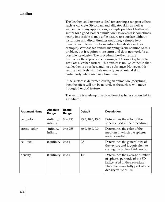
Leather
The Leather solid texture is ideal for creating a range of effects such as concrete, Styrofoam and alligator skin, as well as leather. For many applications, a simple pix file of leather will suffice for a good leather simulation. However, it is sometimes nearly impossible to map a file texture to a surface without distortions and discontinuities (mapping a simple two-dimensional file texture to an automotive dashboard, for example). Worldspace texture mapping is one solution to this problem, but it requires more effort and does not work for all possible topologies. The procedural Leather texture overcomes these problems by using a 3D noise of spheres to simulate a leather surface. This texture is unlike leather in that real leather is a surface, and not a substance. However, this texture can nicely simulate many types of animal skin, particularly when used as a bump map.
If the surface is deformed during an animation (morphing), then the effect will not be natural, as the surface will move through the solid texture.
The texture is made up of a collection of spheres suspended in a medium.
Argument NameAbsolute Range
Useful Range
Default Description
cell_color -infinity, infinity
0 to 255 95.0, 40.0, 15.0 Determines the color of the spheres used in the procedure.
crease_color -infinity, infinity
0 to 255 60.0, 30.0, 0.0 Determines the color of the medium in which the spheres are suspended.
cell_size 0, infinity 0 to 1 0.5 Determines the general size of the texture and is equivalent to scaling the texture DAG node.
density 0, infinity 0 to 1 1.0 Determines the average number of spheres per node of the 3D lattice used in the procedure. The spheres are fully packed at a density value of 1.0.
526
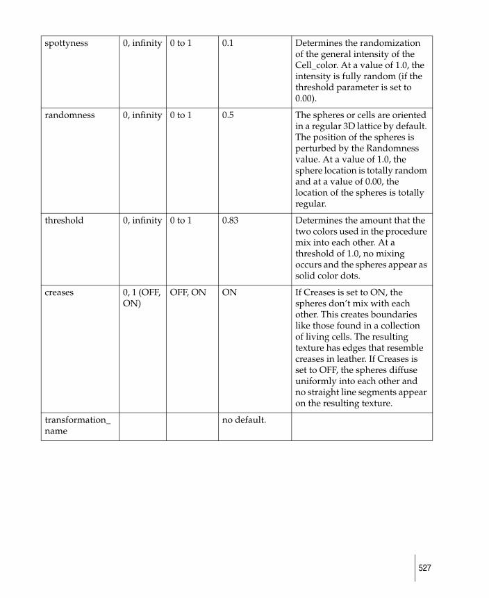
spottyness 0, infinity 0 to 1 0.1 Determines the randomization of the general intensity of the Cell_color. At a value of 1.0, the intensity is fully random (if the threshold parameter is set to 0.00).
randomness 0, infinity 0 to 1 0.5 The spheres or cells are oriented in a regular 3D lattice by default. The position of the spheres is perturbed by the Randomness value. At a value of 1.0, the sphere location is totally random and at a value of 0.00, the location of the spheres is totally regular.
threshold 0, infinity 0 to 1 0.83 Determines the amount that the two colors used in the procedure mix into each other. At a threshold of 1.0, no mixing occurs and the spheres appear as solid color dots.
creases 0, 1 (OFF, ON)
OFF, ON ON If Creases is set to ON, the spheres don’t mix with each other. This creates boundaries like those found in a collection of living cells. The resulting texture has edges that resemble creases in leather. If Creases is set to OFF, the spheres diffuse uniformly into each other and no straight line segments appear on the resulting texture.
transformation_name
no default.
527
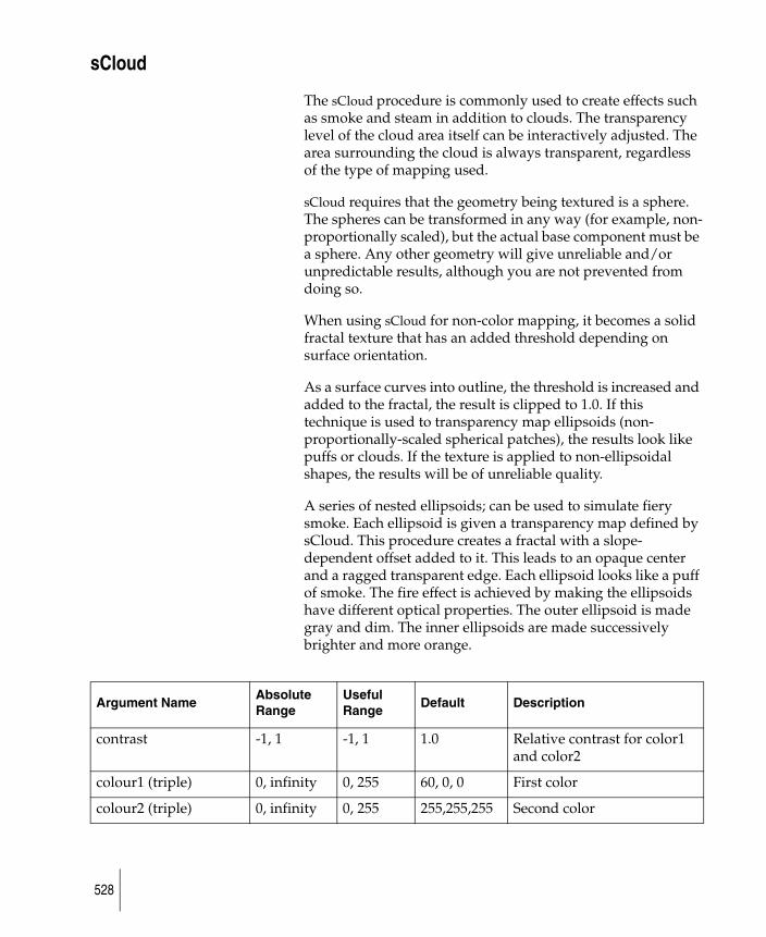
sCloud
The sCloud procedure is commonly used to create effects such as smoke and steam in addition to clouds. The transparency level of the cloud area itself can be interactively adjusted. The area surrounding the cloud is always transparent, regardless of the type of mapping used.
sCloud requires that the geometry being textured is a sphere. The spheres can be transformed in any way (for example, non-proportionally scaled), but the actual base component must be a sphere. Any other geometry will give unreliable and/or unpredictable results, although you are not prevented from doing so.
When using sCloud for non-color mapping, it becomes a solid fractal texture that has an added threshold depending on surface orientation.
As a surface curves into outline, the threshold is increased and added to the fractal, the result is clipped to 1.0. If this technique is used to transparency map ellipsoids (non-proportionally-scaled spherical patches), the results look like puffs or clouds. If the texture is applied to non-ellipsoidal shapes, the results will be of unreliable quality.
A series of nested ellipsoids; can be used to simulate fiery smoke. Each ellipsoid is given a transparency map defined by sCloud. This procedure creates a fractal with a slope-dependent offset added to it. This leads to an opaque center and a ragged transparent edge. Each ellipsoid looks like a puff of smoke. The fire effect is achieved by making the ellipsoids have different optical properties. The outer ellipsoid is made gray and dim. The inner ellipsoids are made successively brighter and more orange.
Argument NameAbsolute Range
Useful Range
Default Description
contrast -1, 1 -1, 1 1.0 Relative contrast for color1 and color2
colour1 (triple) 0, infinity 0, 255 60, 0, 0 First color
colour2 (triple) 0, infinity 0, 255 255,255,255 Second color
528
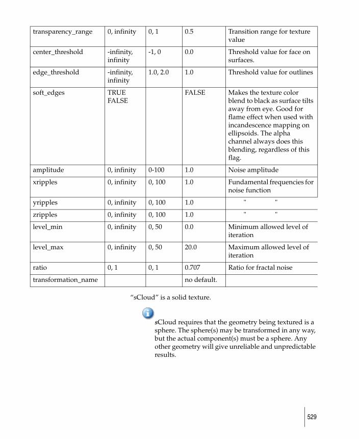
“sCloud” is a solid texture.
sCloud requires that the geometry being textured is a sphere. The sphere(s) may be transformed in any way, but the actual component(s) must be a sphere. Any other geometry will give unreliable and unpredictable results.
transparency_range 0, infinity 0, 1 0.5 Transition range for texture value
center_threshold -infinity, infinity
-1, 0 0.0 Threshold value for face on surfaces.
edge_threshold -infinity, infinity
1.0, 2.0 1.0 Threshold value for outlines
soft_edges TRUE FALSE
FALSE Makes the texture color blend to black as surface tilts away from eye. Good for flame effect when used with incandescence mapping on ellipsoids. The alpha channel always does this blending, regardless of this flag.
amplitude 0, infinity 0-100 1.0 Noise amplitude
xripples 0, infinity 0, 100 1.0 Fundamental frequencies for noise function
yripples 0, infinity 0, 100 1.0 " "
zripples 0, infinity 0, 100 1.0 " "
level_min 0, infinity 0, 50 0.0 Minimum allowed level of iteration
level_max 0, infinity 0, 50 20.0 Maximum allowed level of iteration
ratio 0, 1 0, 1 0.707 Ratio for fractal noise
transformation_name no default.
529
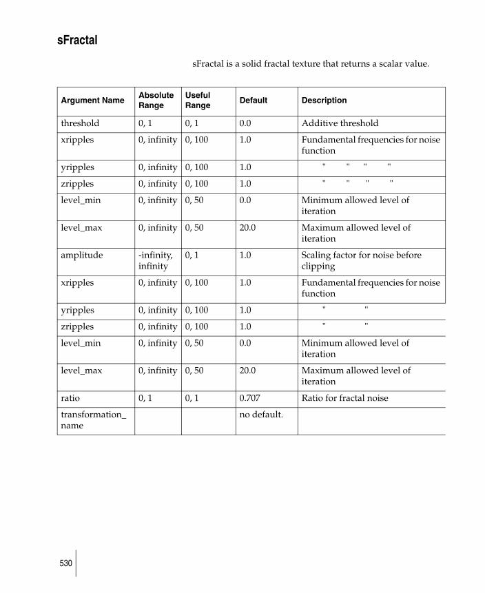
sFractal
sFractal is a solid fractal texture that returns a scalar value.
Argument NameAbsolute Range
Useful Range
Default Description
threshold 0, 1 0, 1 0.0 Additive threshold
xripples 0, infinity 0, 100 1.0 Fundamental frequencies for noise function
yripples 0, infinity 0, 100 1.0 " " " "
zripples 0, infinity 0, 100 1.0 " " " "
level_min 0, infinity 0, 50 0.0 Minimum allowed level of iteration
level_max 0, infinity 0, 50 20.0 Maximum allowed level of iteration
amplitude -infinity, infinity
0, 1 1.0 Scaling factor for noise before clipping
xripples 0, infinity 0, 100 1.0 Fundamental frequencies for noise function
yripples 0, infinity 0, 100 1.0 " "
zripples 0, infinity 0, 100 1.0 " "
level_min 0, infinity 0, 50 0.0 Minimum allowed level of iteration
level_max 0, infinity 0, 50 20.0 Maximum allowed level of iteration
ratio 0, 1 0, 1 0.707 Ratio for fractal noise
transformation_name
no default.
530
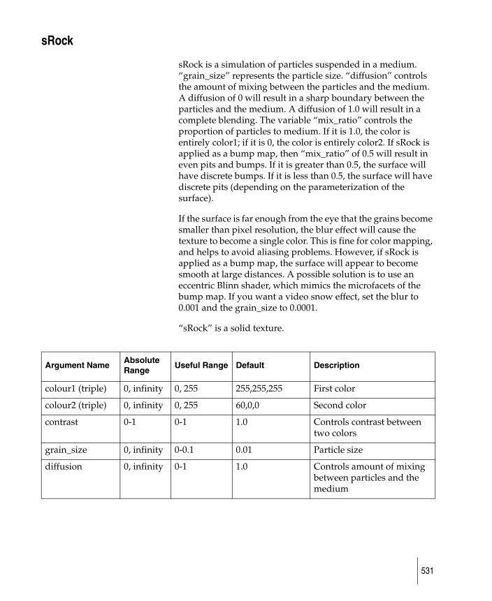
sRock
sRock is a simulation of particles suspended in a medium. “grain_size” represents the particle size. “diffusion” controls the amount of mixing between the particles and the medium. A diffusion of 0 will result in a sharp boundary between the particles and the medium. A diffusion of 1.0 will result in a complete blending. The variable “mix_ratio” controls the proportion of particles to medium. If it is 1.0, the color is entirely color1; if it is 0, the color is entirely color2. If sRock is applied as a bump map, then “mix_ratio” of 0.5 will result in even pits and bumps. If it is greater than 0.5, the surface will have discrete bumps. If it is less than 0.5, the surface will have discrete pits (depending on the parameterization of the surface).
If the surface is far enough from the eye that the grains become smaller than pixel resolution, the blur effect will cause the texture to become a single color. This is fine for color mapping, and helps to avoid aliasing problems. However, if sRock is applied as a bump map, the surface will appear to become smooth at large distances. A possible solution is to use an eccentric Blinn shader, which mimics the microfacets of the bump map. If you want a video snow effect, set the blur to 0.001 and the grain_size to 0.0001.
“sRock” is a solid texture.
Argument NameAbsolute Range
Useful Range Default Description
colour1 (triple) 0, infinity 0, 255 255,255,255 First color
colour2 (triple) 0, infinity 0, 255 60,0,0 Second color
contrast 0-1 0-1 1.0 Controls contrast between two colors
grain_size 0, infinity 0-0.1 0.01 Particle size
diffusion 0, infinity 0-1 1.0 Controls amount of mixing between particles and the medium
531

mix_ratio 0-1 0-1 1.0 Controls the proportion of particles to medium
transformation_name
no default.
532
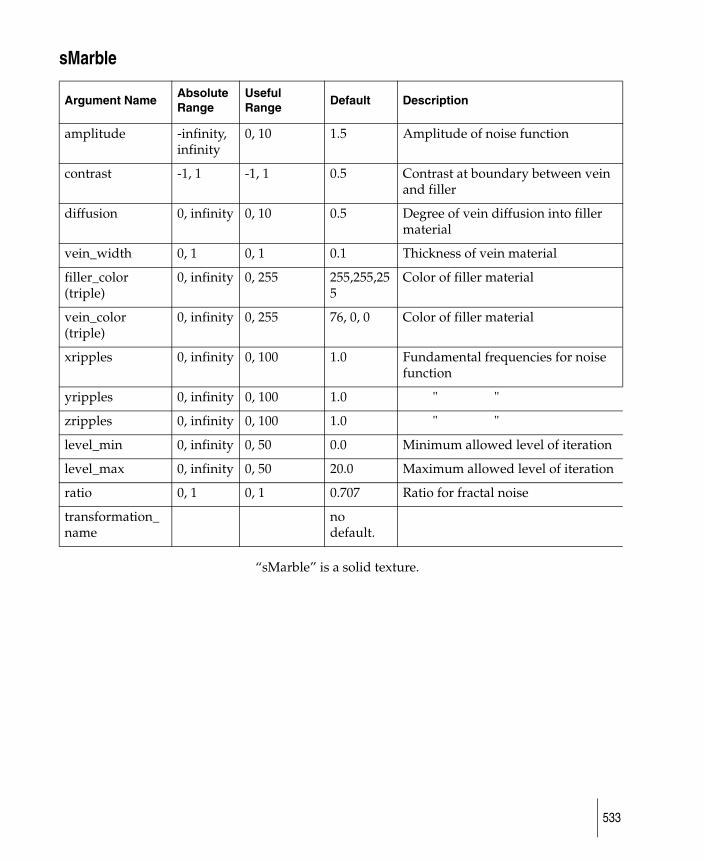
sMarble
“sMarble” is a solid texture.
Argument NameAbsolute Range
Useful Range
Default Description
amplitude -infinity, infinity
0, 10 1.5 Amplitude of noise function
contrast -1, 1 -1, 1 0.5 Contrast at boundary between vein and filler
diffusion 0, infinity 0, 10 0.5 Degree of vein diffusion into filler material
vein_width 0, 1 0, 1 0.1 Thickness of vein material
filler_color (triple)
0, infinity 0, 255 255,255,255
Color of filler material
vein_color (triple)
0, infinity 0, 255 76, 0, 0 Color of filler material
xripples 0, infinity 0, 100 1.0 Fundamental frequencies for noise function
yripples 0, infinity 0, 100 1.0 " "
zripples 0, infinity 0, 100 1.0 " "
level_min 0, infinity 0, 50 0.0 Minimum allowed level of iteration
level_max 0, infinity 0, 50 20.0 Maximum allowed level of iteration
ratio 0, 1 0, 1 0.707 Ratio for fractal noise
transformation_name
no default.
533
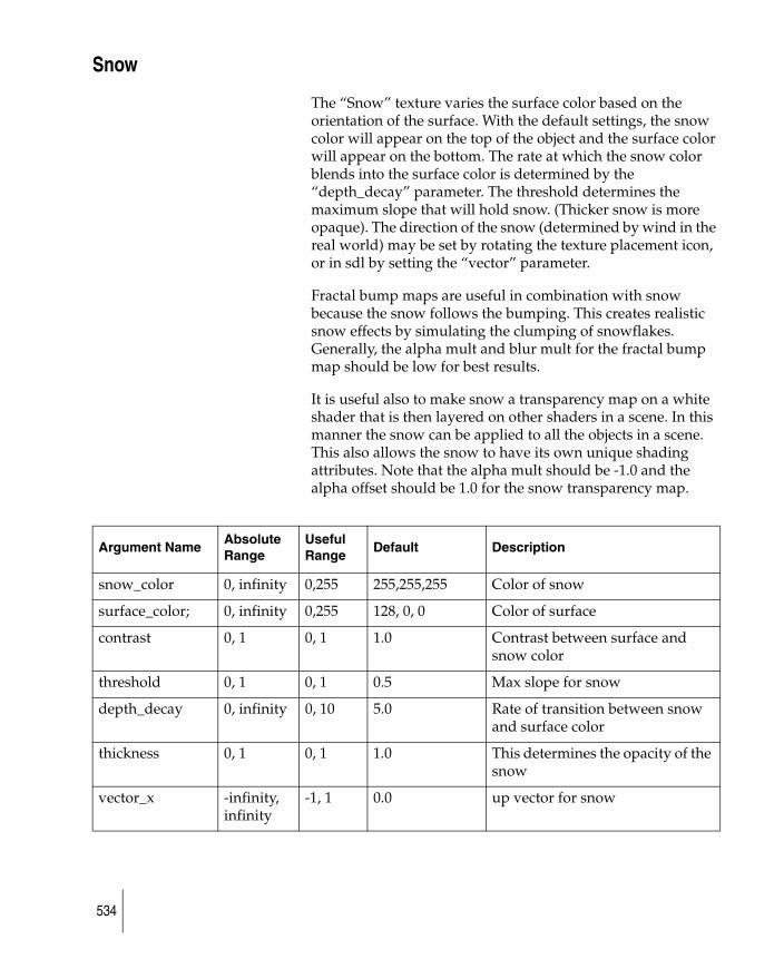
Snow
The “Snow” texture varies the surface color based on the orientation of the surface. With the default settings, the snow color will appear on the top of the object and the surface color will appear on the bottom. The rate at which the snow color blends into the surface color is determined by the “depth_decay” parameter. The threshold determines the maximum slope that will hold snow. (Thicker snow is more opaque). The direction of the snow (determined by wind in the real world) may be set by rotating the texture placement icon, or in sdl by setting the “vector” parameter.
Fractal bump maps are useful in combination with snow because the snow follows the bumping. This creates realistic snow effects by simulating the clumping of snowflakes. Generally, the alpha mult and blur mult for the fractal bump map should be low for best results.
It is useful also to make snow a transparency map on a white shader that is then layered on other shaders in a scene. In this manner the snow can be applied to all the objects in a scene. This also allows the snow to have its own unique shading attributes. Note that the alpha mult should be -1.0 and the alpha offset should be 1.0 for the snow transparency map.
Argument NameAbsolute Range
Useful Range
Default Description
snow_color 0, infinity 0,255 255,255,255 Color of snow
surface_color; 0, infinity 0,255 128, 0, 0 Color of surface
contrast 0, 1 0, 1 1.0 Contrast between surface and snow color
threshold 0, 1 0, 1 0.5 Max slope for snow
depth_decay 0, infinity 0, 10 5.0 Rate of transition between snow and surface color
thickness 0, 1 0, 1 1.0 This determines the opacity of the snow
vector_x -infinity, infinity
-1, 1 0.0 up vector for snow
534

vector_y -infinity, infinity
-1, 1 1.0
vector_z -infinity, infinity
-1, 1 0.0
transformation_name
no default.
535
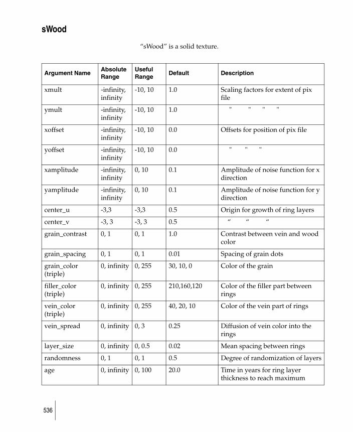
sWood
“sWood” is a solid texture.
Argument NameAbsolute Range
Useful Range
Default Description
xmult -infinity, infinity
-10, 10 1.0 Scaling factors for extent of pix file
ymult -infinity, infinity
-10, 10 1.0 " " " "
xoffset -infinity, infinity
-10, 10 0.0 Offsets for position of pix file
yoffset -infinity, infinity
-10, 10 0.0 " " "
xamplitude -infinity, infinity
0, 10 0.1 Amplitude of noise function for x direction
yamplitude -infinity, infinity
0, 10 0.1 Amplitude of noise function for y direction
center_u -3,3 -3,3 0.5 Origin for growth of ring layers
center_v -3, 3 -3, 3 0.5 “ “ “
grain_contrast 0, 1 0, 1 1.0 Contrast between vein and wood color
grain_spacing 0, 1 0, 1 0.01 Spacing of grain dots
grain_color (triple)
0, infinity 0, 255 30, 10, 0 Color of the grain
filler_color (triple)
0, infinity 0, 255 210,160,120 Color of the filler part between rings
vein_color (triple)
0, infinity 0, 255 40, 20, 10 Color of the vein part of rings
vein_spread 0, infinity 0, 3 0.25 Diffusion of vein color into the rings
layer_size 0, infinity 0, 0.5 0.02 Mean spacing between rings
randomness 0, 1 0, 1 0.5 Degree of randomization of layers
age 0, infinity 0, 100 20.0 Time in years for ring layer thickness to reach maximum
536
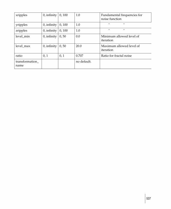
xripples 0, infinity 0, 100 1.0 Fundamental frequencies for noise function
yripples 0, infinity 0, 100 1.0 " "
zripples 0, infinity 0, 100 1.0 " "
level_min 0, infinity 0, 50 0.0 Minimum allowed level of iteration
level_max 0, infinity 0, 50 20.0 Maximum allowed level of iteration
ratio 0, 1 0, 1 0.707 Ratio for fractal noise
transformation_name
no default.
537
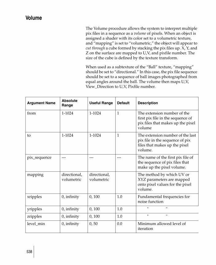
Volume
The Volume procedure allows the system to interpret multiple pix files in a sequence as a volume of pixels. When an object is assigned a shader with its color set to a volumetric texture, and “mapping” is set to “volumetric,” the object will appear to cut through a cube formed by stacking the pix files up. X, Y, and Z on the surface are mapped to U,V, and pixfile number. The size of the cube is defined by the texture transform.
When used as a subtexture of the “Ball” texture, “mapping” should be set to “directional.” In this case, the pix file sequence should be set to a sequence of ball images photographed from equal angles around the ball. The volume then maps U,V, View_Direction to U,V, Pixfile number.
Argument NameAbsolute Range
Useful Range Default Description
from 1-1024 1-1024 1 The extension number of the first pix file in the sequence of pix files that makes up the pixel volume
to 1-1024 1-1024 1 The extension number of the last pix file in the sequence of pix files that makes up the pixel volume.
pix_sequence --- --- --- The name of the first pix file of the sequence of pix files that make up the pixel volume.
mapping directional, volumetric
directional, volumetric
The method by which UV or XYZ parameters are mapped onto pixel values for the pixel volume.
xripples 0, infinity 0, 100 1.0 Fundamental frequencies for noise function
yripples 0, infinity 0, 100 1.0 " "
zripples 0, infinity 0, 100 1.0 " "
level_min 0, infinity 0, 50 0.0 Minimum allowed level of iteration
538

level_max 0, infinity 0, 50 20.0 Maximum allowed level of iteration
ratio 0, 1 0, 1 0.707 Ratio for fractal noise
transformation_name
no default.
539
About environment mapsAn environment map is a model of the world as seen from a particular point of view over a viewing angle of 360°. In StudioTools, environment maps may be used for two things. For reflection mapping, the environment map is used to store a model of the world around a particular point inside or near a surface. This map is then used to compute the color of a ray reflected by that surface. In this way, convincing reflection effects may be produced.
The syntax for using an environment map to do reflections is as follows. In the DEFINITION section use the following statement as part of a texture on a shader:
reflection = texture (procedure = name,
arg 1 = value 1,
arg 2 = value 2,
etc. ...);
The second application of environment maps is to create backgrounds. Since an environment map stores a complete view of the world in all directions, any particular view may be computed efficiently. This will only be accurate if the environment map was created around the current eye point. There are several reasons to do this.
First, the environment may be procedural in nature and this is the only way to see it. The "sky" procedure is a good example of this case. Secondly, a scene may be largely static but also very expensive to render. In that case a fast method for animating the camera direction without re-rendering the scene for every frame would be desirable. Moving objects could then be rendered over the top. The "Cube" procedure would be ideal for this approach. The syntax for creating a background from an environment map is as follows. In the ENVIRONMENT section use:
background = texture (procedure = name,
arg 1 = value 1,
arg 2 = value 2,
etc. ...);
540
An environment map exists in an environment space coordinate system. The default for all environments in StudioTools is to have the environment space aligned with world space. Certain applications require the ability to rotate the environment map relative to world space. In particular, an object, lights and camera may be fixed relative to each other and the environment map tumbled. The syntax for this is identical to the coordinate transformations used with solid textures.
For example, consider a surface that is a ball being rendered with reflection mapping. It needs to have a transformation associated with it.
In the DEFINITION section the transformation must first be declared.
transformation ball;
A subsequent shader will include a textured parameter with “transformation_name”
reflection = texture (procedure = Chrome,
transformation_name= ball),
In the MODEL section the statement
ball = current_transformation ( );
will appear.
If it is located at the base of the hierarchy then the reflection map will be unaffected since the default is for the environment map to be aligned with world space anyway. However, if the assignment of the “current_transformation” to “ball” appears within a hierarchy, the environment map will rotate with the hierarchy. So, if the assignment occurs just before a patch statement the environment map will rotate with the patch. If a non-proportional scale is applied, the environment map will be stretched and distorted.
It is important to note that Ball, Chrome, Cube, Sphere and Sky should not be used for bump or displacement mapping. The basic nature of environment mapping precludes accurate calculations. Although the system will allow it, you will be warned that the results will be unreliable and unpredictable.
541
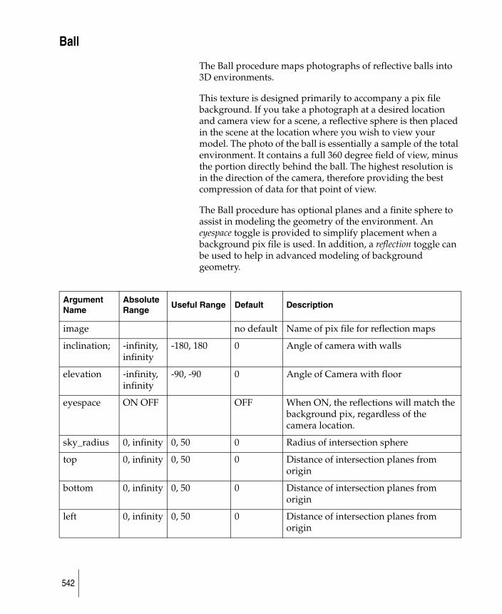
Ball
The Ball procedure maps photographs of reflective balls into 3D environments.
This texture is designed primarily to accompany a pix file background. If you take a photograph at a desired location and camera view for a scene, a reflective sphere is then placed in the scene at the location where you wish to view your model. The photo of the ball is essentially a sample of the total environment. It contains a full 360 degree field of view, minus the portion directly behind the ball. The highest resolution is in the direction of the camera, therefore providing the best compression of data for that point of view.
The Ball procedure has optional planes and a finite sphere to assist in modeling the geometry of the environment. An eyespace toggle is provided to simplify placement when a background pix file is used. In addition, a reflection toggle can be used to help in advanced modeling of background geometry.
Argument Name
Absolute Range
Useful Range Default Description
image no default Name of pix file for reflection maps
inclination; -infinity, infinity
-180, 180 0 Angle of camera with walls
elevation -infinity, infinity
-90, -90 0 Angle of Camera with floor
eyespace ON OFF OFF When ON, the reflections will match the background pix, regardless of the camera location.
sky_radius 0, infinity 0, 50 0 Radius of intersection sphere
top 0, infinity 0, 50 0 Distance of intersection planes from origin
bottom 0, infinity 0, 50 0 Distance of intersection planes from origin
left 0, infinity 0, 50 0 Distance of intersection planes from origin
542
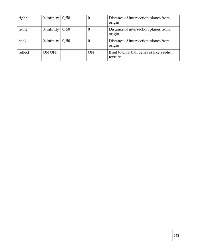
right 0, infinity 0, 50 0 Distance of intersection planes from origin
front 0, infinity 0, 50 0 Distance of intersection planes from origin
back 0, infinity 0, 50 0 Distance of intersection planes from origin
reflect ON OFF ON If set to OFF, ball behaves like a solid texture
543
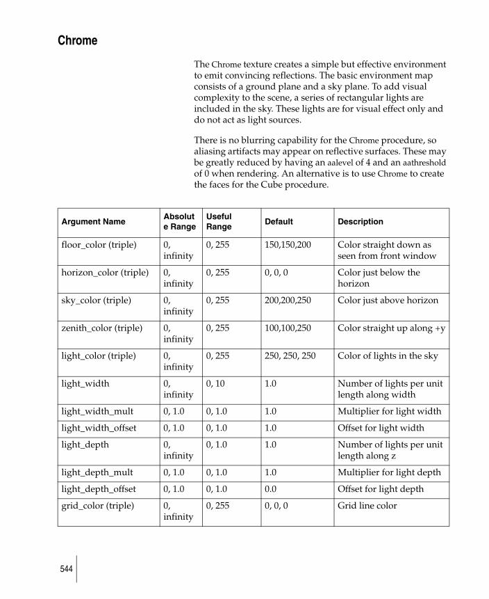
Chrome
The Chrome texture creates a simple but effective environment to emit convincing reflections. The basic environment map consists of a ground plane and a sky plane. To add visual complexity to the scene, a series of rectangular lights are included in the sky. These lights are for visual effect only and do not act as light sources.
There is no blurring capability for the Chrome procedure, so aliasing artifacts may appear on reflective surfaces. These may be greatly reduced by having an aalevel of 4 and an aathreshold of 0 when rendering. An alternative is to use Chrome to create the faces for the Cube procedure.
Argument NameAbsolute Range
Useful Range
Default Description
floor_color (triple) 0, infinity
0, 255 150,150,200 Color straight down as seen from front window
horizon_color (triple) 0, infinity
0, 255 0, 0, 0 Color just below the horizon
sky_color (triple) 0, infinity
0, 255 200,200,250 Color just above horizon
zenith_color (triple) 0, infinity
0, 255 100,100,250 Color straight up along +y
light_color (triple) 0, infinity
0, 255 250, 250, 250 Color of lights in the sky
light_width 0, infinity
0, 10 1.0 Number of lights per unit length along width
light_width_mult 0, 1.0 0, 1.0 1.0 Multiplier for light width
light_width_offset 0, 1.0 0, 1.0 1.0 Offset for light width
light_depth 0, infinity
0, 1.0 1.0 Number of lights per unit length along z
light_depth_mult 0, 1.0 0, 1.0 1.0 Multiplier for light depth
light_depth_offset 0, 1.0 0, 1.0 0.0 Offset for light depth
grid_color (triple) 0, infinity
0, 255 0, 0, 0 Grid line color
544

“Chrome” is an environment texture.
grid_width 0, infinity
0, 10 1.0 Number of grid cells per unit length along x
grid_width_mult 0, 1.0 0, 1.0 1.0 Multiplier for grid width
grid_width_offset 0, 1.0 0, 1.0 0.0 Offset for grid width
grid_depth 0, infinity
0, 10 1.0 Number of grid cells per unit length along z
grid_depth_mult 0, 1.0 0, 1.0 1.0 Multiplier for grid depth
grid_depth_offset 0, 1.0 0, 1.0 0.0 Offset for grid depth
real_floor TRUE FALSE
0, 1 0 Flag for presence of real vs angular floor
floor_altitude -infinity, infinity
-100, 100 -1.0 Elevation of floor along the y-axis
545
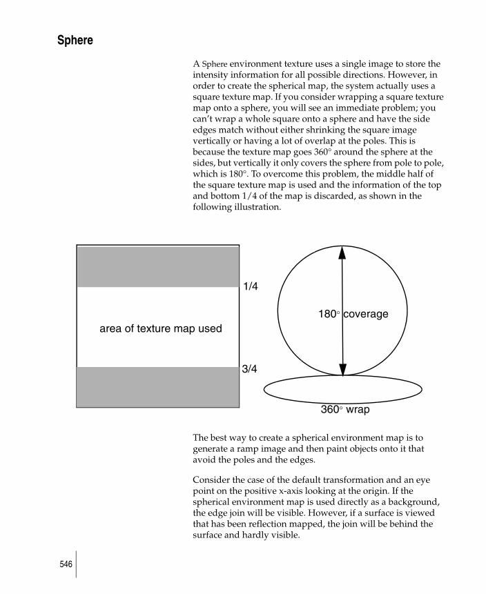
Sphere
A Sphere environment texture uses a single image to store the intensity information for all possible directions. However, in order to create the spherical map, the system actually uses a square texture map. If you consider wrapping a square texture map onto a sphere, you will see an immediate problem; you can’t wrap a whole square onto a sphere and have the side edges match without either shrinking the square image vertically or having a lot of overlap at the poles. This is because the texture map goes 360° around the sphere at the sides, but vertically it only covers the sphere from pole to pole, which is 180°. To overcome this problem, the middle half of the square texture map is used and the information of the top and bottom 1/4 of the map is discarded, as shown in the following illustration.
The best way to create a spherical environment map is to generate a ramp image and then paint objects onto it that avoid the poles and the edges.
Consider the case of the default transformation and an eye point on the positive x-axis looking at the origin. If the spherical environment map is used directly as a background, the edge join will be visible. However, if a surface is viewed that has been reflection mapped, the join will be behind the surface and hardly visible.
360° wrap
180° coveragearea of texture map used
1/4
3/4
546
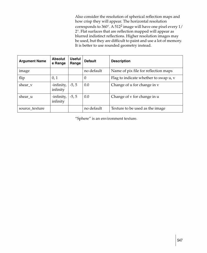
Also consider the resolution of spherical reflection maps and how crisp they will appear. The horizontal resolution corresponds to 360°. A 5122 image will have one pixel every 1/2°. Flat surfaces that are reflection mapped will appear as blurred indistinct reflections. Higher resolution images may be used, but they are difficult to paint and use a lot of memory. It is better to use rounded geometry instead.
“Sphere” is an environment texture.
Argument NameAbsolute Range
Useful Range
Default Description
image no default Name of pix file for reflection maps
flip 0, 1 0 Flag to indicate whether to swap u, v
shear_v -infinity, infinity
-5, 5 0.0 Change of u for change in v
shear_u -infinity, infinity
-5, 5 0.0 Change of v for change in u
source_texture no default Texture to be used as the image
547
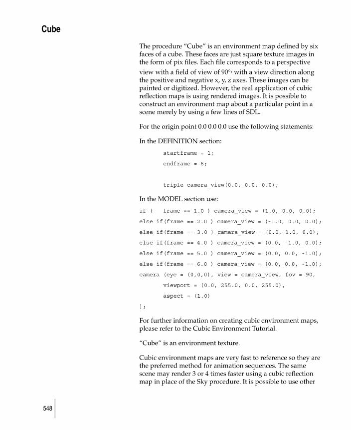
Cube
The procedure “Cube” is an environment map defined by six faces of a cube. These faces are just square texture images in the form of pix files. Each file corresponds to a perspective view with a field of view of 90°, with a view direction along the positive and negative x, y, z axes. These images can be painted or digitized. However, the real application of cubic reflection maps is using rendered images. It is possible to construct an environment map about a particular point in a scene merely by using a few lines of SDL.
For the origin point 0.0 0.0 0.0 use the following statements:
In the DEFINITION section:
startframe = 1;
endframe = 6;
triple camera_view(0.0, 0.0, 0.0);
In the MODEL section use:
if ( frame == 1.0 ) camera_view = (1.0, 0.0, 0.0);
else if(frame == 2.0 ) camera_view = (-1.0, 0.0, 0.0);
else if(frame == 3.0 ) camera_view = (0.0, 1.0, 0.0);
else if(frame == 4.0 ) camera_view = (0.0, -1.0, 0.0);
else if(frame == 5.0 ) camera_view = (0.0, 0.0, -1.0);
else if(frame == 6.0 ) camera_view = (0.0, 0.0, -1.0);
camera (eye = (0,0,0), view = camera_view, fov = 90,
viewport = (0.0, 255.0, 0.0, 255.0),
aspect = (1.0)
);
For further information on creating cubic environment maps, please refer to the Cubic Environment Tutorial.
“Cube” is an environment texture.
Cubic environment maps are very fast to reference so they are the preferred method for animation sequences. The same scene may render 3 or 4 times faster using a cubic reflection map in place of the Sky procedure. It is possible to use other
548
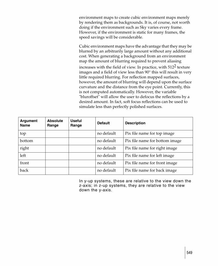
environment maps to create cubic environment maps merely by rendering them as backgrounds. It is, of course, not worth doing if the environment such as Sky varies every frame. However, if the environment is static for many frames, the speed savings will be considerable.
Cubic environment maps have the advantage that they may be blurred by an arbitrarily large amount without any additional cost. When generating a background from an environment map the amount of blurring required to prevent aliasing increases with the field of view. In practice, with 5122 texture images and a field of view less than 90° this will result in very little required blurring. For reflection mapped surfaces, however, the amount of blurring will depend upon the surface curvature and the distance from the eye point. Currently, this is not computed automatically. However, the variable "bluroffset" will allow the user to defocus the reflections by a desired amount. In fact, soft focus reflections can be used to simulate less than perfectly polished surfaces.
In y-up systems, these are relative to the view down the z-axis; in z-up systems, they are relative to the view down the y-axis.
Argument Name
Absolute Range
Useful Range
Default Description
top no default Pix file name for top image
bottom no default Pix file name for bottom image
right no default Pix file name for right image
left no default Pix file name for left image
front no default Pix file name for front image
back no default Pix file name for back image
549
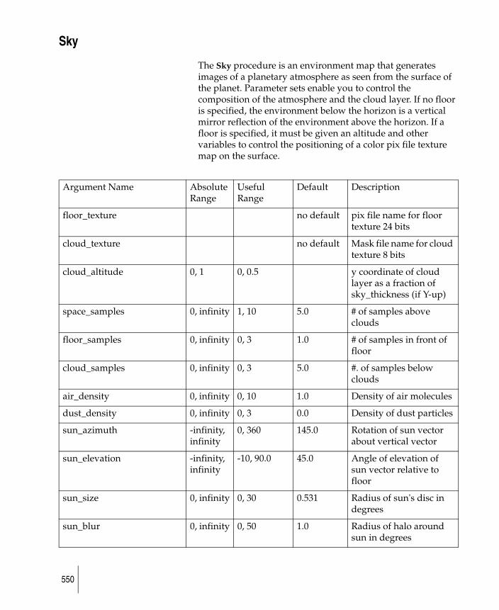
Sky
The Sky procedure is an environment map that generates images of a planetary atmosphere as seen from the surface of the planet. Parameter sets enable you to control the composition of the atmosphere and the cloud layer. If no floor is specified, the environment below the horizon is a vertical mirror reflection of the environment above the horizon. If a floor is specified, it must be given an altitude and other variables to control the positioning of a color pix file texture map on the surface.
Argument Name Absolute Range
Useful Range
Default Description
floor_texture no default pix file name for floor texture 24 bits
cloud_texture no default Mask file name for cloud texture 8 bits
cloud_altitude 0, 1 0, 0.5 y coordinate of cloud layer as a fraction of sky_thickness (if Y-up)
space_samples 0, infinity 1, 10 5.0 # of samples above clouds
floor_samples 0, infinity 0, 3 1.0 # of samples in front of floor
cloud_samples 0, infinity 0, 3 5.0 #. of samples below clouds
air_density 0, infinity 0, 10 1.0 Density of air molecules
dust_density 0, infinity 0, 3 0.0 Density of dust particles
sun_azimuth -infinity, infinity
0, 360 145.0 Rotation of sun vector about vertical vector
sun_elevation -infinity, infinity
-10, 90.0 45.0 Angle of elevation of sun vector relative to floor
sun_size 0, infinity 0, 30 0.531 Radius of sun's disc in degrees
sun_blur 0, infinity 0, 50 1.0 Radius of halo around sun in degrees
550
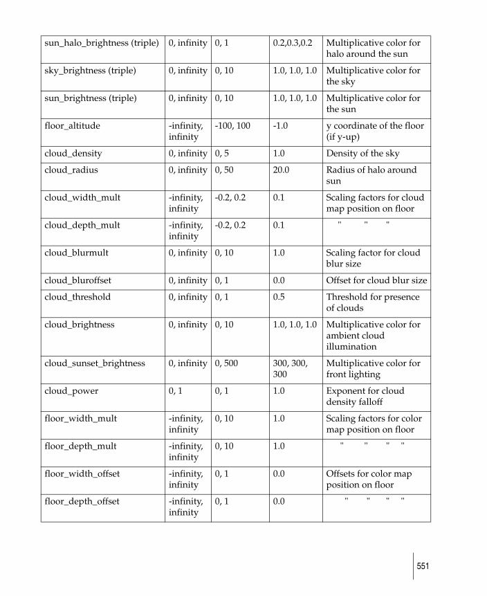
sun_halo_brightness (triple) 0, infinity 0, 1 0.2,0.3,0.2 Multiplicative color for halo around the sun
sky_brightness (triple) 0, infinity 0, 10 1.0, 1.0, 1.0 Multiplicative color for the sky
sun_brightness (triple) 0, infinity 0, 10 1.0, 1.0, 1.0 Multiplicative color for the sun
floor_altitude -infinity, infinity
-100, 100 -1.0 y coordinate of the floor (if y-up)
cloud_density 0, infinity 0, 5 1.0 Density of the sky
cloud_radius 0, infinity 0, 50 20.0 Radius of halo around sun
cloud_width_mult -infinity, infinity
-0.2, 0.2 0.1 Scaling factors for cloud map position on floor
cloud_depth_mult -infinity, infinity
-0.2, 0.2 0.1 " " "
cloud_blurmult 0, infinity 0, 10 1.0 Scaling factor for cloud blur size
cloud_bluroffset 0, infinity 0, 1 0.0 Offset for cloud blur size
cloud_threshold 0, infinity 0, 1 0.5 Threshold for presence of clouds
cloud_brightness 0, infinity 0, 10 1.0, 1.0, 1.0 Multiplicative color for ambient cloud illumination
cloud_sunset_brightness 0, infinity 0, 500 300, 300, 300
Multiplicative color for front lighting
cloud_power 0, 1 0, 1 1.0 Exponent for cloud density falloff
floor_width_mult -infinity, infinity
0, 10 1.0 Scaling factors for color map position on floor
floor_depth_mult -infinity, infinity
0, 10 1.0 " " " "
floor_width_offset -infinity, infinity
0, 1 0.0 Offsets for color map position on floor
floor_depth_offset -infinity, infinity
0, 1 0.0 " " " "
551
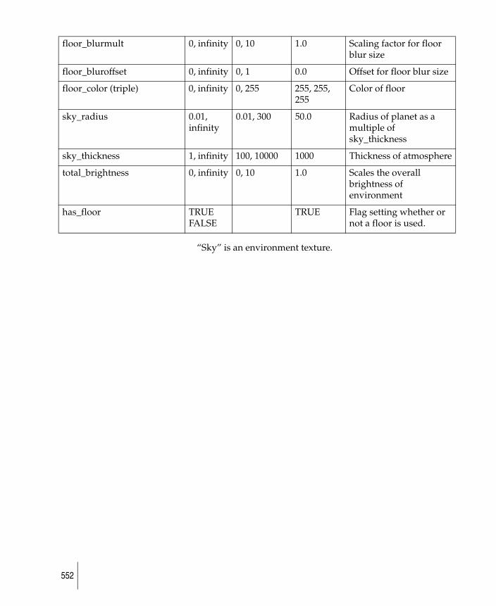
“Sky” is an environment texture.
floor_blurmult 0, infinity 0, 10 1.0 Scaling factor for floor blur size
floor_bluroffset 0, infinity 0, 1 0.0 Offset for floor blur size
floor_color (triple) 0, infinity 0, 255 255, 255, 255
Color of floor
sky_radius 0.01, infinity
0.01, 300 50.0 Radius of planet as a multiple of sky_thickness
sky_thickness 1, infinity 100, 10000 1000 Thickness of atmosphere
total_brightness 0, infinity 0, 10 1.0 Scales the overall brightness of environment
has_floor TRUE FALSE
TRUE Flag setting whether or not a floor is used.
552

Tutorials
553
Creating Rendered Cubic Environment MapsCubic environment maps provide a fast and attractive way to simulate a one-bounce ray trace. The object to which a cubic environment (sometimes called a cubic reflection) map is applied, appears to reflect its environment. This tutorial will demonstrate a method for creating cubic environment maps for two types of reflections. The first will show how to create the reflection map for a non-planar object in the scene, and the second will show how to create a reflection map for a reflective plane (i.e., a floor or a wall).
Road Map
The basic steps involved in creating the reflection map files are as follows:
1 Copy the original SDL file to a different “special” SDL file.
2 Edit the special SDL file, remove the object that we are creating the reflection map for.
3 Change the name of the output file.
4 Change the eye position, twist, fov, resolution and aspect ratio
5 Add the animation of the view direction
6 Finish editing the special SDL file.
7 Render the special SDL file.
8 Edit the original SDL file to add the reflection map to the proper shader.
9 Render the original SDL file.
Reflection Map for a Non-planar Object in the Scene
A cubic environment map requires six pix files that show what is seen along each of the positive and negative axes directions from a spiced point. It is the specification of the point that
554
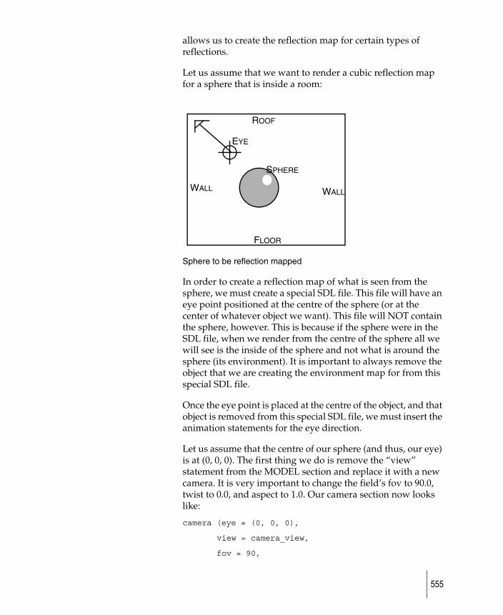
allows us to create the reflection map for certain types of reflections.
Let us assume that we want to render a cubic reflection map for a sphere that is inside a room:
Sphere to be reflection mapped
In order to create a reflection map of what is seen from the sphere, we must create a special SDL file. This file will have an eye point positioned at the centre of the sphere (or at the center of whatever object we want). This file will NOT contain the sphere, however. This is because if the sphere were in the SDL file, when we render from the centre of the sphere all we will see is the inside of the sphere and not what is around the sphere (its environment). It is important to always remove the object that we are creating the environment map for from this special SDL file.
Once the eye point is placed at the centre of the object, and that object is removed from this special SDL file, we must insert the animation statements for the eye direction.
Let us assume that the centre of our sphere (and thus, our eye) is at (0, 0, 0). The first thing we do is remove the “view” statement from the MODEL section and replace it with a new camera. It is very important to change the field’s fov to 90.0, twist to 0.0, and aspect to 1.0. Our camera section now looks like:
camera (eye = (0, 0, 0),
view = camera_view,
fov = 90,
ROOF
EYE
SPHERE
WALLWALL
FLOOR
555
viewport = (0.0, 255.0, 0.0, 255.0),
aspect = (1.0)
);
In order to use this camera, it must be defined in the DEFINITION section:
triple camera_view (0.0, 0.0, 0.0);
In order to create the pix files from this little animation, the DEFINITION section must include:
startframe = 1;
endframe = 6;
It is also important to remember that we are creating pix files that are to be used as texture maps, so the resolution should be one of 256, 512, 1024, etc.
The final step is to add animation to the MODEL section, also as described in this manual:
if ( frame == 1.0 ) camera_view = (1.0, 0.0, 0.0);
else if(frame == 2.0 ) camera_view = (-1.0, 0.0, 0.0);
else if(frame == 3.0 ) camera_view = (0.0, 1.0, 0.0);
else if(frame == 4.0 ) camera_view = (0.0, -1.0, 0.0);
else if(frame == 5.0 ) camera_view = (0.0, 0.0, -1.0);
else if(frame == 6.0 ) camera_view = (0.0, 0.0, 1.0);
After rendering this special SDL file, we return to the original SDL file and add the reflection map to the shader that corresponds to the object (in this case, a sphere).
shader AAA ( model = phong,
diffuse = 0.800000,
shinyness = 10.000000,
color = (0.0, 0.0, 0.0),
specular = (0.800000, 0.800000, 0.800000),
reflectivity = 1.0,
556
reflection = texture(procedure = Cube,
right = "pix/special.1",
left = "pix/special.2",
top = "pix/special.3",
bottom = "pix/special.4",
front = "pix/special.6",
back = "pix/special.5"
)
);
The sphere will now have a reflection of the environment on it.
Reflection Map for a Reflective Plane
The first section described how to create and use a reflection map for an object in the scene. Creating reflection maps for planar objects (say a shiny floor) is done in a different manner.
Creating a reflection map for a planar object is easiest if the planar object lies on one of the XY, YZ, or XZ planes. If this is not the case, then calculation of the eye point for the special SDL file is difficult, but it can still be done.
Let’s start with the simplest case. We have a planar object that lies on the XZ plane (see below). For simplicity, we will refer to this planar object as the floor of our modeled room, in a Y-up environment.
557
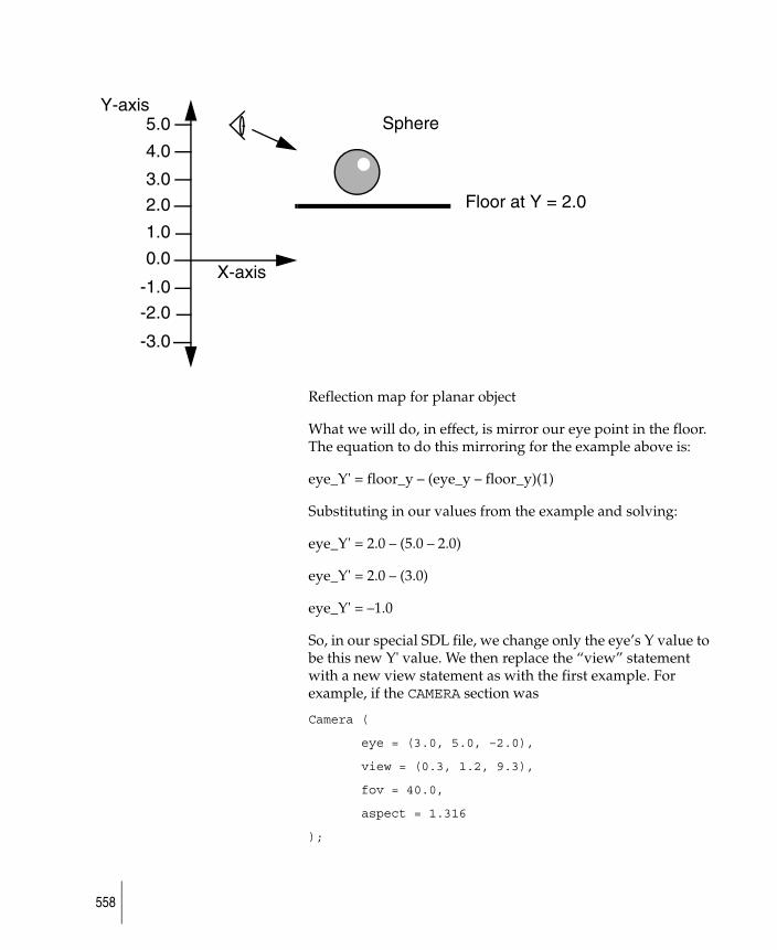
Reflection map for planar object
What we will do, in effect, is mirror our eye point in the floor. The equation to do this mirroring for the example above is:
eye_Y' = floor_y – (eye_y – floor_y)(1)
Substituting in our values from the example and solving:
eye_Y' = 2.0 – (5.0 – 2.0)
eye_Y' = 2.0 – (3.0)
eye_Y' = –1.0
So, in our special SDL file, we change only the eye’s Y value to be this new Y' value. We then replace the “view” statement with a new view statement as with the first example. For example, if the CAMERA section was
Camera (
eye = (3.0, 5.0, –2.0),
view = (0.3, 1.2, 9.3),
fov = 40.0,
aspect = 1.316
);
Floor at Y = 2.0
Sphere
X-axis
Y-axis5.0
4.0
3.0
2.0
1.0
0.0
-1.0
-2.0
-3.0
558
then we would change it to
camera (
eye = (3.0, -1.0, –2.0),
view = camera_view,
fov = 90,
viewport = (0.0, 255.0, 0.0, 255.0),
aspect = (1.0)
);
and, as before, we would change the output pixel resolution to one of 256, 512, 1024, 2048, etc., and add the animation to the MODEL section for x_dir, y_dir, and z_dir. This special SDL file is rendered and the reflection map is applied to the floor’s surface descriptor in the original SDL file. Remember to remove the floor in the special SDL.
If the planar object is not on the XZ plane, then the modified coordinate can be found by substitution of X for Y in equation (1) if the object lies in the YZ plane or by substituting Z for Y in equation (1) if the object lies in the XY plane.
If the planar object does not lie in one of the above planes, then it becomes more difficult to calculate the new eye point, and it requires a lot more math.
Let’s say that our planar object is described as a face that has the following points in the SDL file:
XYZ
V1–0.4183–4.642.5132
V2–3.905–1.0842.5716
V30.1143.2474–1.6657
V44.1738–0.3513–2.0018
And assume that the eye is at (0.5, 0.5, 12).
Now, in order to reflect the eye point in this plane, we will need a normal to this plane. To calculate the normal, we need 3 of the vertices of the planar object. Let us arbitrarily choose V1, V2 and V3, which from inspection of the wire frame, we know
559
do not lie in a straight line (in mathematical terms, the points are not co-linear).
DX2 = V2.X – V1.X(2)
DX3 = V3.X – V1.X(3)
DY2 = V2.Y – V1.Y(4)
DY3 = V3.Y – V1.Y(5)
DZ2 = V2.Z – V1.Z(6)
DZ3 = V3.Z – V1.Z(7)
The results of equations (2) through (7) are then used to compute:
L = DY2 *DZ3 – DY3 * DZ2(8)
M = DX3 * DZ2 – DX2 * DZ3(9)
N = DX2 * DY3 – DX3 * DY2(10)
R = L * L + M * M + N * N(11)
R = SQRT(R)(12)
L = L/R(13)
M = M/R(14)
N = N/R(15)
P = L * V1.X + M * V1.Y + N * V1.Z(16)
Now, you might think that all of that is far too much math for one day, but we’re not done yet. (SQRT(R) in equation (12) means that we want the square root of the number represented by R.)
The distance of the eye point from this plane is calculated by:
D = L * EYE_X + M * EYE_Y + N * EYE_Z + P(17)
If D is negative, then the new eye point is given by:
D = 2 * (–D)
560
EYE_X' = EYE_X + D * L(18)
EYE_Y' = EYE_Y + D * M
EYE_Z' = EYE_Z + D * N
If D is positive, then the new eye point is given by:
D = 2 * D
EYE_X' = EYE_X + D * (–L)(19)
EYE_Y' = EYE_Y + D * (–M)
EYE_Z' = EYE_Z + D * (–N)
If D turns out to be equal to 0.0, then the eye point is on the plane and you should not create a reflection map for this object, because a mirror viewed “side on” does not reflect anything.
Returning to our example and placing the values into equations (2) through (7) we get:
DX2 = –3.905 – –0.4183 =-3.4867
DX3 = 0.114 – –0.4183 =0.5323
DY2 = –1.084 – –4.64 =3.556
DY3 = 3.2474 – –4.64 =7.8874
DZ2 = 2.5716 – 2.5132 =0.584
DZ3 = –1.6657 – 2.5132 = –4.1789
Placing these values into equations (8) through (10) we get:
L = 3.556 * –4.1789 – 7.8874 * 0.584=-19.46641
M = 0.5323 * 0.584 – –3.4867 * –4.1789=–14.2597
N = –3.4867 * 7.8874 – 0.5323 * 3.556=–29.39385
Using these values in equations (11) and (12) we get:
561
R = –19.46641 * –19.46641 + –14.2597 * –14.2597 + –29.39385 * –29.39385
= 1446.27858
R = SQRT (1446.27858) = 38.02997
Then applying equations (13) to (15) we get:
L = –19.46641/38.02997 =–0.51187
M = –14.2597/38.02997=–0.37496
N = –29.39385/38.02997=–0.77291
Then we take a break to catch our breath and continue by applying equation (16) to these numbers:
P = –0.51187 * –0.4183 + –0.37496 * –4.64 + –0.77291 * 2.5132 = 0.011452
After applying equation (17) we get:
D = –0.51187 * 0.5 + –0.37496 * 0.5 + –0.77291 * 12.0 + 0.011452 = –9.70688
We can see that D is negative, so we apply equation (18):
D = 2 * (– –9.70688) = 2 * 9.70688 = 19.41376
Note that the negative of a negative number is a positive number, and continue with equation (18):
EYE_X' = 0.5 + 19.41376 * –0.51187 = –9.43732
EYE_Y' = 0.5 + 19.41376 * –0.37496 = –6.77938
EYE_Z' = 12.0 + 19.41376 * –0.77291 = –3.0051
Now that we have our new eye point, we go back to our special SDL file, and replace all three eye components:
eye = (–9.43732, –6.77938, –3.0051),
And again, as before, we replace the rest of the camera data, set the proper resolution, add the animation to the MODEL
562
section and render this special SDL file to create the reflection map.
Notes and Limitations
Shadows do not show up on surfaces that get all of their color from a reflection map. In order for a shadow to appear on a reflection-mapped surface, the surface must have a non-zero diffuse value.
A reflection-mapped object does not reflect itself. For example, a teapot will not reflect its spout, but it will reflect the rest of the scene. This is because we have to remove the object which will reflect from the special SDL file we create. To get proper reflections of an object with itself requires ray tracing. This method provides a cheaper alternative to ray tracing.
The methods for creating reflection maps described in this tutorial are for a static object in the “reflection maps for an object” case and for a static object and eye in the “reflection maps for planar surfaces” case. Should you wish to create high quality reflections for a moving object in an animation, then a new reflection map will have to be created for each frame of the animation. In the case of planar objects, some time can be saved by noting that some of the reflection map views do not “see” anything and are therefore black. These views only need to be created once for the entire animation.
563
Creating projectile movement
Cross Reference
“An Introduction to Dynamics,” a companion tutorial, is strongly recommended.
General Principles
Projectiles are objects which have an initial velocity and then move in a way which depends on the forces acting on them.
The total force f acting on a mass m creates an acceleration a according to the following equation:
f = ma
In a time step, , the new velocity can be derived
from the old velocity using:
where is the instantaneous acceleration. The new position
is given by:
These formulae assume that is very small.
Projectiles have an initial velocity and an initial position
. The force acting on the particle is computed taking into
account gravity and atmospheric drag, and the motion path for the projectile results. The equations above work for each coordinate independently.
∆t vi 1+vi
vi 1+ vi ai∆t+=
ai
xi 1+ xi Vi∆t 12---ai ∆t( )2+ +=
∆t
v0x0
564
Terrestrial Cannon Ball
For a terrestrial cannon ball the effects of gravity are uniform. The force of gravity acts down along the y axis and is proportional to the mass.
This is Galileo's famous discovery that, in the absence of an atmosphere, all objects fall with the same acceleration. (A cannon ball and a feather hit the ground at the same time if released from the same height on the moon!).
The SDL file CourseWare/SDL/proj simulates a projectile moving through a vacuum. The initial velocities along x and y are computed from a total velocity and an angle of elevation. Try changing the angle to see which angle gives the maximum range for the projectile. Range is defined as the distance it moves through before returning to its initial y value.
Real projectiles, however, move through air. This slows them along their path by creating a frictional force which acts in the opposite direction to the velocity of the projectile (relative to the wind).
Therefore,
The SDL file CourseWare/SDL/dproj simulates this effect. Try different values of “drag.” Is the optimal elevation angle still 45°?
The effect of the atmospheric drag is to reduce the horizontal velocity eventually to zero, and to slow the ball both in its rise and descent. The ball ultimately ends up descending vertically at a "terminal" velocity. The force of gravity is then equal to the atmospheric drag.
f gravity mass×=
a gravity massmass------------×=
a gravity=
f gravity mass drag velocity×–×=
565
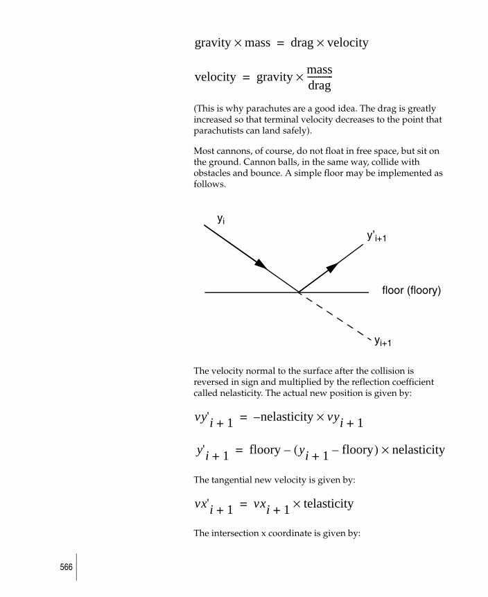
(This is why parachutes are a good idea. The drag is greatly increased so that terminal velocity decreases to the point that parachutists can land safely).
Most cannons, of course, do not float in free space, but sit on the ground. Cannon balls, in the same way, collide with obstacles and bounce. A simple floor may be implemented as follows.
The velocity normal to the surface after the collision is reversed in sign and multiplied by the reflection coefficient called nelasticity. The actual new position is given by:
The tangential new velocity is given by:
The intersection x coordinate is given by:
gravity mass× drag velocity×=
velocity gravity massdrag------------×=
yi
y’i+1
floor (floory)
yi+1
vy'i 1+ nelasticity vyi 1+×–=
y'i 1+ floory yi 1+ floory–( ) nelasticity×–=
vx'i 1+ vxi 1+ telasticity×=
566
The next x coordinate for the particle is:
This model is implemented in the SDL file CourseWare/SDL/cproj. Try changing the different values of the elasticities.
Roman Candle
While individual projectiles are useful in some circumstances, the true power of procedural animation is revealed when a large number of objects are involved. Consider a roman candle with a spray of sparks issuing from it. Each particle will follow a trajectory that depends on its initial velocity and position. The current velocity and position of each particle have to be stored in SDL variables. This is made easy by defining arrays with an index that refers to the particle number.
The SDL file CourseWare/SDL/roman illustrates how to create a firework of exactly this sort. A looping "for" structure is used to process each particle in turn. The variable "numpart" controls the number of particles in the animation sequence; 10000 is plenty but they take a long time to animate and will not play back in real time using preview. A "numpart" of 300 should prove adequate for motion tests. The individual particles are modeled as cylinders which extend from the previous position to the current one. The rendering is additive, i.e. the cylinders are completely transparent with a colored incandescence value. It happens that when large numbers of such particles are rendered on top of each other, the color clips to white. This works rather nicely for the firework.
Unfortunately, the "wireframe" rendering mode uses the color value for the particles. The color value of these particles is actually black. This will lead to black particles on a black background. For wireframe tests, it is necessary to make the color white.
The wind velocity is a global control over the animation. Every particle is affected along its trajectory. The SDL file
xcxi xi 1+ xi–( ) floory yi–( )×+
yi 1+ yi–( )----------------------------------------------------------------------------=
x'i 1+ xc xi 1+ xc–( ) telasticity×+=
567
CourseWare/SDL/roman uses an animate statement to control the wind as a function of time. The wind blows to the right strongly early in the animation and then gusts less later on. Try experimenting with the drag coefficient, the particle velocities and the amount of gravity. Try moving the spark origin point as a function of the birth time to simulate a rocket.
Snow Storm
A snow storm may be thought of as a collection of particles. They are created in a condensation or cloud layer. The flakes will have randomly distributed positions and will then fall under gravity. Some flakes will have different drag coefficients and so will fall at different rates. They will also tumble randomly as they fall.
This model is implemented in the SDL file CourseWare/SDL/snow. When rendered, the snow flakes, which are faces, are transparency mapped with images which were derived from photographs of real snow flakes. The wind direction is chosen to be perpendicular to the direction of view. This prevented any snow flakes from blowing too close to the camera and so looking enormous. A useful trick was also employed to prevent the system from running out of snow flakes. The viewing frustum was considered to be looking through an active volume of snow fall. The left and right sides of the volume were outside of the field of view. This volume was defined by ± xrang and ± zrang. Any snow flakes which passed out of the positive x wall were moved to the corresponding spot on the negative x wall. In this way the number of snow flakes was used to best effect.
568
Programming Movement with Constraints
Piston Rod Example
Inverse kinematics is a technique for generating the joint angles for a hierarchy in a way that fulfills geometrical constraints. A constraint is something which reduces the freedom of movement of an object. For instance, a cylinder in a cylinder block is constrained to one degree of freedom, i.e. sliding along its length.
If a piston rod is to pivot both on a wheel and a cylinder, and the cylinder is to be constrained linearly, then the system only
has one degree of freedom. The rotation angle at A determines the angle at B which in turn determines the position of C.
A simple two-dimensional hierarchy has two degrees of freedom. It is the constraint of the cylinder which makes the
angle at B dependent on and reduces the degrees of freedom to 1. Computing such dependencies is the focus of inverse kinematics. This requires inverse trigonometric functions and Pythagoras' Theorem.
θ
θ
569
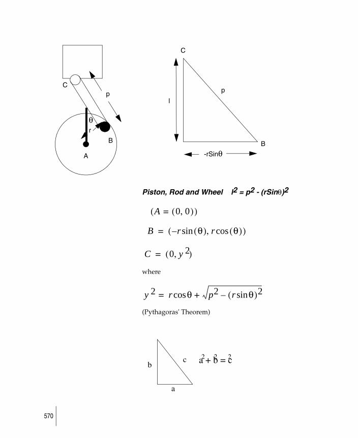
Piston, Rod and Wheel l2 = p2 - (rSinθ)2
where
(Pythagoras' Theorem)
A
B
C
B
C
p
l
-rSinθ
θr
p
A 0 0,( )=( )
B r θ( ) r θ( )cos,sin–( )=
C 0 y 2,( )=
y 2 r θcos p2 r θsin( )2–+=
a
bc a + b = c22 2
570
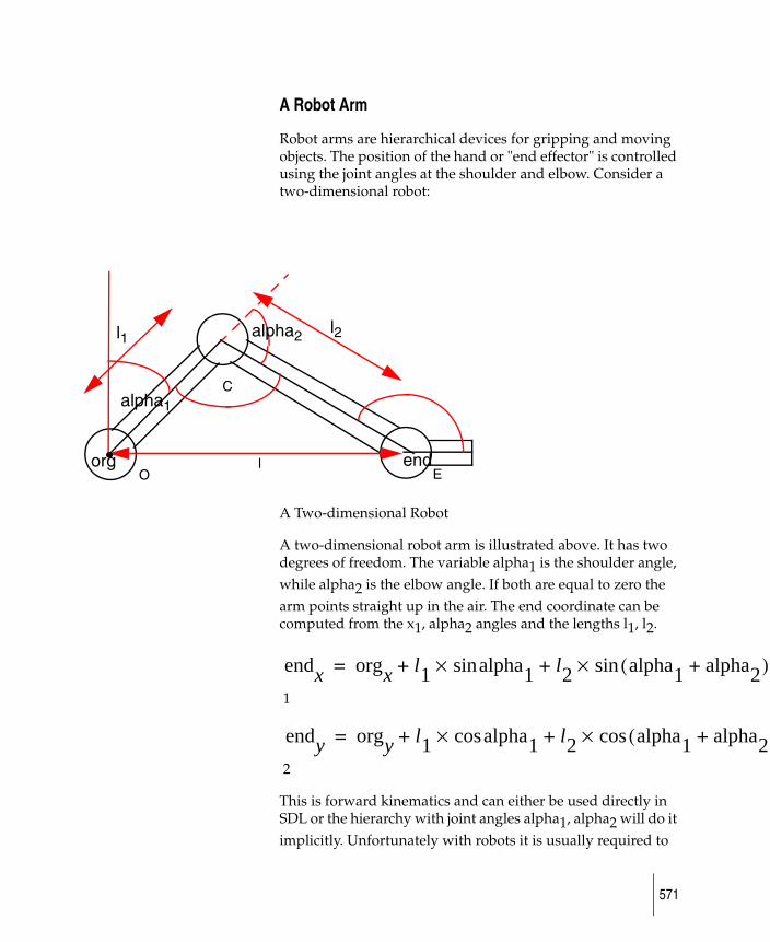
alpha2)
alpha2+ )
A Robot Arm
Robot arms are hierarchical devices for gripping and moving objects. The position of the hand or "end effector" is controlled using the joint angles at the shoulder and elbow. Consider a two-dimensional robot:
A Two-dimensional Robot
A two-dimensional robot arm is illustrated above. It has two degrees of freedom. The variable alpha1 is the shoulder angle, while alpha2 is the elbow angle. If both are equal to zero the arm points straight up in the air. The end coordinate can be computed from the x1, alpha2 angles and the lengths l1, l2.
1
2
This is forward kinematics and can either be used directly in SDL or the hierarchy with joint angles alpha1, alpha2 will do it implicitly. Unfortunately with robots it is usually required to
endorg
alpha1
alpha2 l2l1
EOl
C
endx orgx l1 alpha1sin× l2 alpha1 +(sin×+ +=
endy orgy l1 alpha1cos× l2 alpha1(cos×+ +=
571
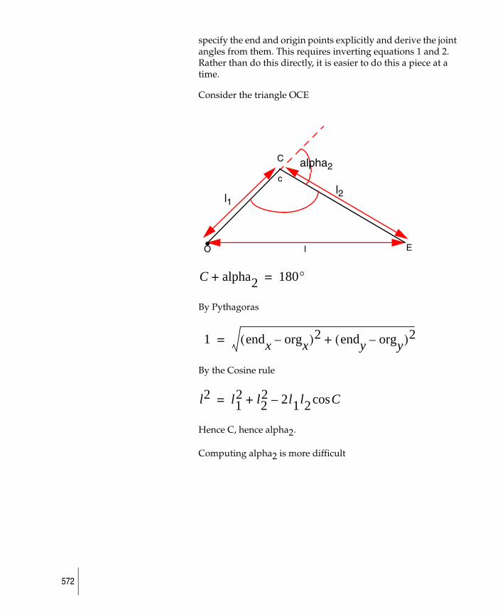
specify the end and origin points explicitly and derive the joint angles from them. This requires inverting equations 1 and 2. Rather than do this directly, it is easier to do this a piece at a time.
Consider the triangle OCE
By Pythagoras
By the Cosine rule
Hence C, hence alpha2.
Computing alpha2 is more difficult
alpha2
l2l1
EO l
C
c
C alpha2+ 180°=
1 endx orgx–( )2 endy orgy–( )2+=
l2 l12 l2
2 2l1l2 Ccos–+=
572
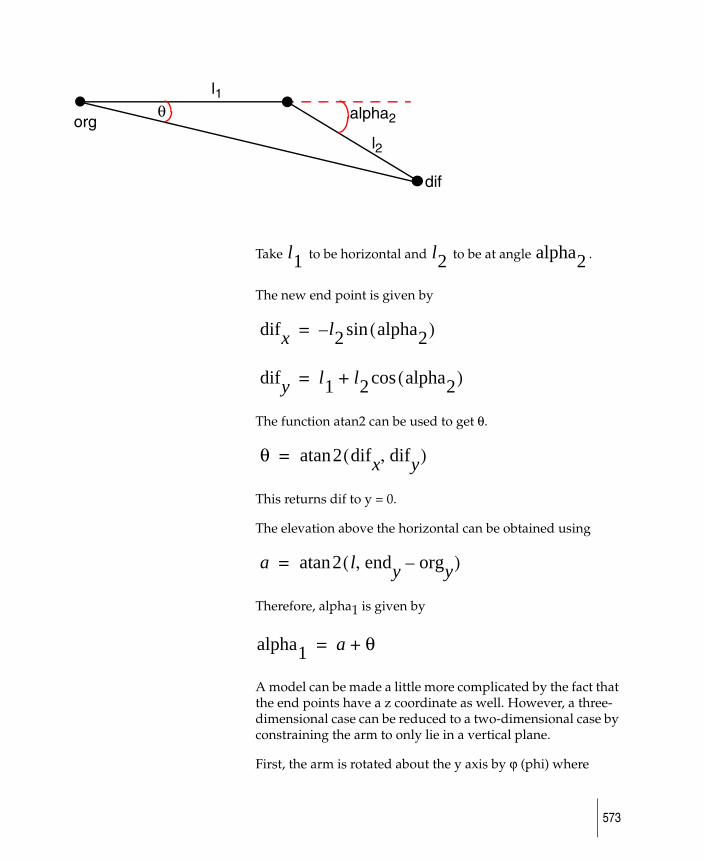
Take to be horizontal and to be at angle .
The new end point is given by
The function atan2 can be used to get θ.
This returns dif to y = 0.
The elevation above the horizontal can be obtained using
Therefore, alpha1 is given by
A model can be made a little more complicated by the fact that the end points have a z coordinate as well. However, a three-dimensional case can be reduced to a two-dimensional case by constraining the arm to only lie in a vertical plane.
First, the arm is rotated about the y axis by ϕ (phi) where
alpha2
l2
dif
orgθ
l1
l1 l2 alpha2
difx l2 alpha2( )sin–=
dify l1 l2 alpha2( )cos+=
θ 2 difx dify,( )atan=
a 2 l endy orgy–,( )atan=
alpha1 a θ+=
573
then the two-dimensional equations are solved as before.
The arm so far described stops at the wrist. A real robot has a gripper which can rotate on a ball joint about the wrist.
This may be achieved again using atan2 functions. The robot arm in this example has a target point called (xtarget, ytarget, ztarget). The wrist is positioned at a point defined by the approach vector (xtarget + xapproach, ytarget + yapproach, ztarget + zapproach). The "gripper", which in fact is just a cylinder, always points towards the target.
Try moving the target point outside the reach of the robot. What happens? Try changing the lengths of the segments.
ϕ 2 endz orgz endx orgx–,––( )atan=
574
An Introduction to Dynamics
General Approach: Mass Spring Systems
Dynamics, in its common usage, just means change. In computer graphics it has a specialized meaning which refers to the way that objects with mass behave when subjected to forces.
A point mass m when subjected to a force, ƒ, will experience an acceleration, a, in accordance with the following equation:
A point mass originally at rest will have an increase in velocity, v, defined by:
where means increment in time and means change in velocity.
At the same time the velocity will cause a change in position:
Therefore, it is possible to find the new position based on the previous position for each step. Thinking of the variables at increment i and increment i + 1:
The force ƒ was shown as ƒ(x) which means that the force is a function of position, e.g.:
f ma=
∆v a∆t=
∆t ∆v
∆x v∆t=
ai 1+f x( )m
---------=
vi 1+ vi ai 1= ∆t+=
xi 1+ xi vi 1+ ∆t 12ai 1+ ∆t-----------------------+ +=
575
This means that a mass at positive x will experience a force pulling it towards the origin. If the mass is at negative x the mass will also be pulled towards the origin. A mass released at position x = p will oscillate around the origin. The force simulates the effect of a spring. The value of k determines how stiff the spring is. The larger the value of k, the stiffer the spring and the faster the oscillation. Experiment usinge a wireframe to create preview files. Try different values of k. The frequency will change. Try different values of mass. What effects does this have?
Damping
A mass on a perfect spring will oscillate forever. In practice, though, real world devices experience friction and atmospheric drag. This may be simulated by modifying the force acting on the mass, making it a function of the object’s velocity as well as position:
where k is the spring constant and d is the damping. The larger the damping value, the more the mass is slowed along its path. Too little damping and the mass oscillates around the origin. Intermediate “critical” damping means that the system comes to rest in the shortest time. Too much damping means that the system gradually comes to rest.
Try a damping value of -0.5. The system gradually gains energy going faster and faster. Negative damping corresponds to unstable systems. Such things do occur in real life; for instance, a bridge in certain wind conditions may oscillate until it fails. There is another source of instability which is due to the way we are computing motion. The use of discrete time steps is only an approximation. The smaller the time step the more accurate the solution. The mass overshoots where it should be and experiences a greater restoring force than it should. It then overshoots the other way. Oscillations build up and, for more complex objects, the system shakes itself to pieces. This problem may be overcome in two ways. The first is to decrease the time step: this may be achieved by having many subintervals per frame of animation.
f x( ) kx–=
f kx– dv–=
576
This enhances the accuracy of the animation and is vital for fast moving effects. Unfortunately, the more subintervals used, the more expensive the solution, and this can be prohibitive if large numbers of objects are involved. The instability may be counteracted by increasing the damping in the system. Too much damping will lead to altered behaviour; too little and the system becomes unstable and “blows up.”
Extending to More Dimensions — Animating a Chain
The previous spring example was only in one dimension. Most problems of interest work in two or three dimensions.
A force that varies as a function of the distance between two point masses may be expressed as follows:
where and and are vectors, and r is the distance between the point masses. n should be set to -1 for a spring, and 2 for gravity.
This may be expressed in terms of components as follows:
for points (x1, y1, z1,) and (x2, y2, z2),
The force along x, y, z acting on particle 1 will be:
A damping term should be proportional to relative motion along the line joining the two masses. This may be achieved by computing the dot product of the difference in position with the difference in velocity:
f krn----- p1 p2–
r------------------⎝ ⎠⎛ ⎞=
f p1 p2
f =( ) krn 1+---------------
f1x x1 x2–( ) f×=
f1y y1 y2–( ) f×=
f1z z1 z2–( ) f×=
577
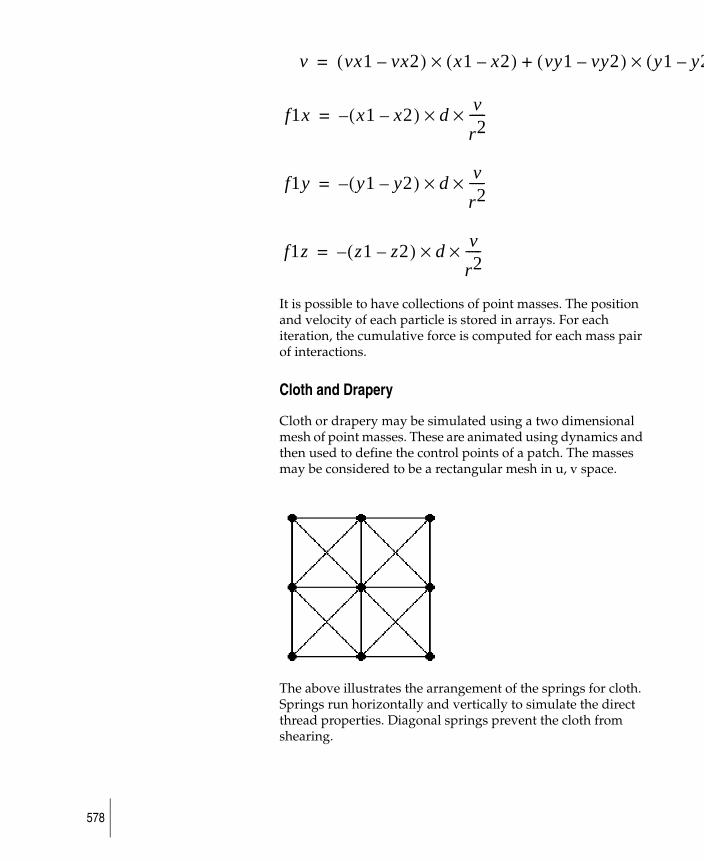
1 y2– ) vz(+
It is possible to have collections of point masses. The position and velocity of each particle is stored in arrays. For each iteration, the cumulative force is computed for each mass pair of interactions.
Cloth and Drapery
Cloth or drapery may be simulated using a two dimensional mesh of point masses. These are animated using dynamics and then used to define the control points of a patch. The masses may be considered to be a rectangular mesh in u, v space.
The above illustrates the arrangement of the springs for cloth. Springs run horizontally and vertically to simulate the direct thread properties. Diagonal springs prevent the cloth from shearing.
v vx1 vx2–( ) x1 x2–( ) vy1 vy2–( ) y(×+×=
f1x x1 x2–( ) d vr2-----××–=
f1y y1 y2–( ) d vr2-----××–=
f1z z1 z2–( ) d vr2-----××–=
578
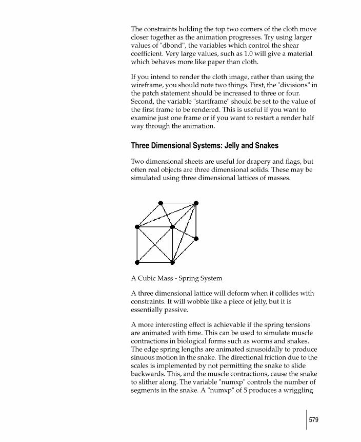
The constraints holding the top two corners of the cloth move closer together as the animation progresses. Try using larger values of "dbond", the variables which control the shear coefficient. Very large values, such as 1.0 will give a material which behaves more like paper than cloth.
If you intend to render the cloth image, rather than using the wireframe, you should note two things. First, the "divisions" in the patch statement should be increased to three or four. Second, the variable "startframe" should be set to the value of the first frame to be rendered. This is useful if you want to examine just one frame or if you want to restart a render half way through the animation.
Three Dimensional Systems: Jelly and Snakes
Two dimensional sheets are useful for drapery and flags, but often real objects are three dimensional solids. These may be simulated using three dimensional lattices of masses.
A Cubic Mass - Spring System
A three dimensional lattice will deform when it collides with constraints. It will wobble like a piece of jelly, but it is essentially passive.
A more interesting effect is achievable if the spring tensions are animated with time. This can be used to simulate muscle contractions in biological forms such as worms and snakes. The edge spring lengths are animated sinusoidally to produce sinuous motion in the snake. The directional friction due to the scales is implemented by not permitting the snake to slide backwards. This, and the muscle contractions, cause the snake to slither along. The variable "numxp" controls the number of segments in the snake. A "numxp" of 5 produces a wriggling
579

grub-like motion but is quite fast. A "numxp" of 30 gives a truly convincing snake and takes considerably more time.
As an exercise, try applying a lifting force to one end of the snake and see the resulting movement.
580
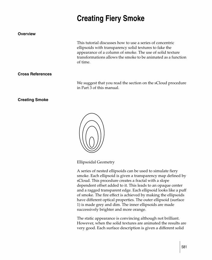
Creating Fiery Smoke
Overview
This tutorial discusses how to use a series of concentric ellipsoids with transparency solid textures to fake the appearance of a column of smoke. The use of solid texture transformations allows the smoke to be animated as a function of time.
Cross References
We suggest that you read the section on the sCloud procedure in Part 3 of this manual.
Creating Smoke
Ellipsoidal Geometry
A series of nested ellipsoids can be used to simulate fiery smoke. Each ellipsoid is given a transparency map defined by sCloud. This procedure creates a fractal with a slope dependent offset added to it. This leads to an opaque center and a ragged transparent edge. Each ellipsoid looks like a puff of smoke. The fire effect is achieved by making the ellipsoids have different optical properties. The outer ellipsoid (surface 1) is made grey and dim. The inner ellipsoids are made successively brighter and more orange.
The static appearance is convincing although not brilliant. However, when the solid textures are animated the results are very good. Each surface description is given a different solid
581

texture transformation which allows the smoke effects to move at different rates.
Try scaling all of the transformations using scales of 10 and 0.1. What effect does this have on the appearance? How does the edge threshold affect the extent of the smoke?
582
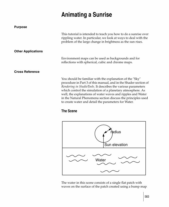
Animating a Sunrise
Purpose
This tutorial is intended to teach you how to do a sunrise over rippling water. In particular, we look at ways to deal with the problem of the large change in brightness as the sun rises.
Other Applications
Environment maps can be used as backgrounds and for reflections with spherical, cubic and chrome maps.
Cross Reference
You should be familiar with the explanation of the "Sky" procedure in Part 3 of this manual, and in the Shader section of Rendering in StudioTools. It describes the various parameters which control the simulation of a planetary atmosphere. As well, the explanations of water waves and ripples and Water in the Natural Phenomena section discuss the principles used to create water and detail the parameters for Water.
The Scene
The water in this scene consists of a single flat patch with waves on the surface of the patch created using a bump map
radius
Sun elevation
Water
583
of the Water procedure. This patch stretches from -200 to 200 units along the x and z axes. This ensures that, when viewed from the eye point, the water plane stretches to the horizon.
The background is a direct view of the procedural environment "Sky". This is also used as a reflection map on the patch to show the sky reflected in the water.
The Animation
There are several primary processes in the animation. The first is the movement of the water waves across the patch. The second is the movement of the sun as it rises above the horizon. The third is the translation of the clouds across the sky. The clouds also become thinner as the day progresses. A secondary process in the animation is the use of the brightness variables to compensate for the enormous changes of brightness which occur during a sunrise.
Each of these processes is now discussed in some detail.
Animating the Water
Since relative displacement maps affect the underlying geometry, to get a realistic level of detail a very high level of subdivision would have to be used; to get around this, a bump map was used instead, and an "amult" value of 0.01 was chosen. The choice of small amplitude waves avoided the expense of using a displacement map instead of a bump map. The large extent of the water patch would have required "urepeat" and "vrepeat" to be 300 for the individual nearby waves to look a reasonable size. This, in turn, would have led to the need for udivisions and vdivisions for the patch of about 1000. This would generate so many triangles that the renderer would run out of memory. A bump map, on the other hand, affects the normal at the point of intersection and leaves the geometry unchanged, so the entire area can be characterized using the minimal two triangles (udivisions and vdivisions of 1).
The "wave_frequency_step" of 0.125 was chosen so as to have several waveforms of almost the same frequency superimposed on top of each other. Large values lead to repetitive, unattractive waves.
584
The "wave_time" is made of a function of the frame number "frame". In this way the waves move smoothly from frame to frame. The "blurmult" and "bluroffset" values mean that the water is sampled in a very small area to compute the slope. This prevents the water from looking flat near the horizon. The only correct way to antialias bump maps is to supersample them everywhere. Blurring the bump map texture merely blurs out the detail. An "aathreshold" of zero ensures supersampling for every pixel. The "aalevel" of 2 was chosen since it reduced aliasing artifacts without making the rendering time completely prohibitive.
Animating the Sun
The sun position is defined in terms of azimuth and elevation angles with respect to the earth. Since the real world rotates, the sun moves across the sky. The correct astronomical animation would be to rotate these angles at a uniform speed. However, for this animation we want the sun to rise quickly at the beginning, and gradually come to a stop. This was achieved by using an ease function.
The field of view for this animation was chosen to be 90°. This has the advantage that large color changes take place over an angle of 90° for a more striking image. However, the large fov has several disadvantages. First, if the sun were to have its real diameter of 1/2°, it would be tiny on the screen. Secondly, a sphere near the edge of a perspective image projects onto the screen as an ellipse, not a circle. This effect gets worse as the field of view increases.
Unfortunately an elliptical sun looks wrong. Fortunately there is an optical effect in the real world's atmosphere which bulges the sun horizontally for low elevations. Thus an "aspect" ratio was chosen which made the sun circular when high in the sky and squashed when low in the sky. If other pieces of geometry are rendered at the same time, they may be laterally distorted, but for this animation it worked.
The sun radius value is changed to compensate for the elongation. It is also much larger than the real sun would appear.
585
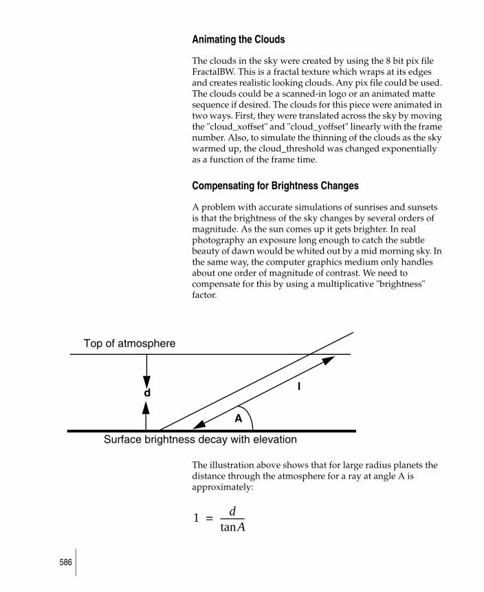
Animating the Clouds
The clouds in the sky were created by using the 8 bit pix file FractalBW. This is a fractal texture which wraps at its edges and creates realistic looking clouds. Any pix file could be used. The clouds could be a scanned-in logo or an animated matte sequence if desired. The clouds for this piece were animated in two ways. First, they were translated across the sky by moving the "cloud_xoffset" and "cloud_yoffset" linearly with the frame number. Also, to simulate the thinning of the clouds as the sky warmed up, the cloud_threshold was changed exponentially as a function of the frame time.
Compensating for Brightness Changes
A problem with accurate simulations of sunrises and sunsets is that the brightness of the sky changes by several orders of magnitude. As the sun comes up it gets brighter. In real photography an exposure long enough to catch the subtle beauty of dawn would be whited out by a mid morning sky. In the same way, the computer graphics medium only handles about one order of magnitude of contrast. We need to compensate for this by using a multiplicative "brightness" factor.
The illustration above shows that for large radius planets the distance through the atmosphere for a ray at angle A is approximately:
d
A
l
Top of atmosphere
Surface brightness decay with elevation
1 dAtan
-----------=
586
A, in this example, is equivalent to the sun's elevation. The brightness decays exponentially with the distance through the atmosphere. However, for this example, the brightness was made proportional to 1/(l + c) where c prevented the brightness becoming infinite for l = 0. This compensation works fairly well, although the sun does flare up slightly half way through the animation. You can try more sophisticated compensation, although we suggest that you investigate these effects using non-antialiased very low resolution images.
A Caveat About Rendering Times
Both "Water" and "Sky" are very expensive procedures. The water model which covers half the screen, is time consuming because it is a time dependent procedure which treats each frequency separately. This time is proportional to the area of the water in screen space. For an NTSC image with an anti-aliasing level (aalevel) of 2 and an anti-aliasing threshold (aathreshold) of zero, the water procedure adds twenty minutes to the rendering time on an SGI 4D workstation.
The sky procedure is also extremely costly. It involves a double integral through the atmosphere. For the same NTSC image, as above, having the sky both as a reflection map on the water and as a background, adds forty minutes to the rendering time on an SGI 4D workstation.
At an hour per frame you may ask why bother? The answers are two-fold. First, the results are rather beautiful and second, the sky procedure will be better understood. One particular time of day (sun elevation) may be rendered once into a cubic environment map and then used for backgrounds and reflections for an entire animation sequence. That is not done here because we change the sky parameters as a function of time.
587
Creating a Tree
Overview
This tutorial describes the use of "for" loops and nested transformations to create a fir tree. The model developed here uses differential equations to simulate the growth of branches. This allows the animation of a tree growing from sapling to adult.
Branching and Looping
A tree may be described as a trunk with branches. On each branch are other branches, etc.
The loop for each branch is as follows:
{
Create a branch
loop for each sub-branch
{
create a sub-branch
loop for each pine needle
{
create a sub-sub-branch
}
}
}
Almost any tree model will have such a structure. The trick is to know how to position the sub-branches on each branch and how many to create. The positioning is comparatively simple if the branching structure is also used to control the transformation hierarchy: then the branches only need to be rotated about their origin and then translated along the branch.
588
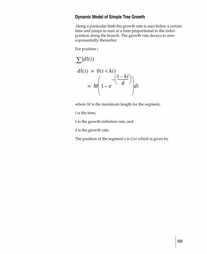
Dynamic Model of Simple Tree Growth
Along a particular limb the growth rate is zero below a certain time and jumps to max at a time proportional to the index position along the branch. The growth rate decays to zero exponentially thereafter.
For position i
where M is the maximum length for the segment,
t is the time,
k is the growth initiation rate, and
d is the growth rate.
The position of the segment a is L(a) which is given by
|dl i( )∑dl i( ) 0 t ki<( )=
M 1 e
t ki–d
------------⎝ ⎠⎛ ⎞–
–⎝ ⎠⎜ ⎟⎜ ⎟⎛ ⎞
di=
589
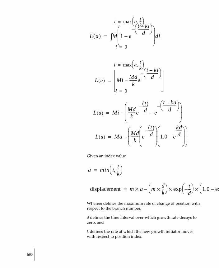
.0 exp kad
------⎝ ⎠⎛ ⎞– ⎠
⎞
Given an index value
Wherem defines the maximum rate of change of position with respect to the branch number,
d defines the time interval over which growth rate decays to zero, and
k defines the rate at which the new growth initiator moves with respect to position index.
L a( ) M 1 e
t ki–d
------------⎝ ⎠⎛ ⎞–
–⎝ ⎠⎜ ⎟⎜ ⎟⎛ ⎞
di∫=
L a( ) Mi Mdk
--------e
t ki–d
------------⎝ ⎠⎛ ⎞–
–=
L a( ) Mi Mdk
--------et( )d
------–e
t ka–d
-------------⎝ ⎠⎛ ⎞–
–⎝ ⎠⎜ ⎟⎜ ⎟⎛ ⎞
–=
L a( ) Ma Mdk
-------- et( )d
------–
⎝ ⎠⎜ ⎟⎜ ⎟⎛ ⎞
1.0 ekdd
------–
⎝ ⎠⎜ ⎟⎜ ⎟⎛ ⎞
⎝ ⎠⎜ ⎟⎜ ⎟⎛ ⎞
–=
i max a tk--,⎝ ⎠
⎛ ⎞=
i 0=
i max a tk--,⎝ ⎠
⎛ ⎞=
i 0=
a min i tk--,⎝ ⎠
⎛ ⎞=
displacement m a m dk---×⎝ ⎠
⎛ ⎞ exp td---–⎝ ⎠
⎛ ⎞ 1⎝⎛××–×=
590
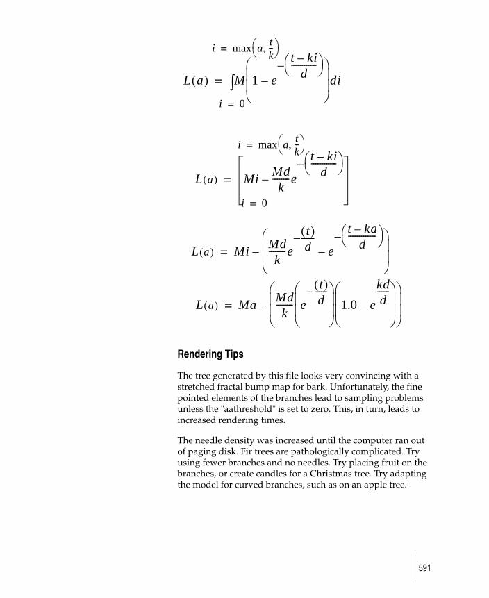
Rendering Tips
The tree generated by this file looks very convincing with a stretched fractal bump map for bark. Unfortunately, the fine pointed elements of the branches lead to sampling problems unless the "aathreshold" is set to zero. This, in turn, leads to increased rendering times.
The needle density was increased until the computer ran out of paging disk. Fir trees are pathologically complicated. Try using fewer branches and no needles. Try placing fruit on the branches, or create candles for a Christmas tree. Try adapting the model for curved branches, such as on an apple tree.
L a( ) M 1 e
t ki–d
------------⎝ ⎠⎛ ⎞–
–⎝ ⎠⎜ ⎟⎜ ⎟⎛ ⎞
di∫=
L a( ) Mi Mdk
--------e
t ki–d
------------⎝ ⎠⎛ ⎞–
–=
L a( ) Mi Mdk
--------et( )d
------–e
t ka–d
-------------⎝ ⎠⎛ ⎞–
–⎝ ⎠⎜ ⎟⎜ ⎟⎛ ⎞
–=
L a( ) Ma Mdk
-------- et( )d
------–
⎝ ⎠⎜ ⎟⎜ ⎟⎛ ⎞
1.0 ekdd
------–
⎝ ⎠⎜ ⎟⎜ ⎟⎛ ⎞
⎝ ⎠⎜ ⎟⎜ ⎟⎛ ⎞
–=
i max a tk--,⎝ ⎠
⎛ ⎞=
i 0=
i max a tk--,⎝ ⎠
⎛ ⎞=
i 0=
591
Creating Rendered Stereo PairsTo create stereo, run-length-encoded images for display on the Stereographics monitor, several changes must be made to an ordinary SDL file.
DEFINITION Section Changes for stereo pairs
First, a flag must be set in the DEFINITION section to have the renderer create a stereo pair. The syntax for it is:
stereo = <scalar>;
where the value of the scalar is 0 (FALSE) or not 0 (TRUE).
The setting of these variables can be performed in the interactive package through the camera editor.
The stereo flag specifies if the camera(s) is to render a stereo pair of images. If this component is TRUE, the pix and mask components (if specified) will have two file names generated for the left and right images.
The generated names will be,
"<specified_name>_left"
"<specified_name>_right"
The “left” and “right” correspond to the output pix files for the left and right eyes. The filename may be animated like other animated filenames (i.e., “basename”extension_expression). If the extension expression is missing and the rendering is an animation, the name will have a standard frame extension. Any extension is appended after the suffixes "_left" and "_right".
For example, if the SDL contained camera (pix="pix/abc",... and it were animated, the renderer would create two pix files for the first frame,
"pix/abc_left.1" and "pix/abc_right.1"
One other variable must be set:
stereo_eye_offset = <scalar>;
592
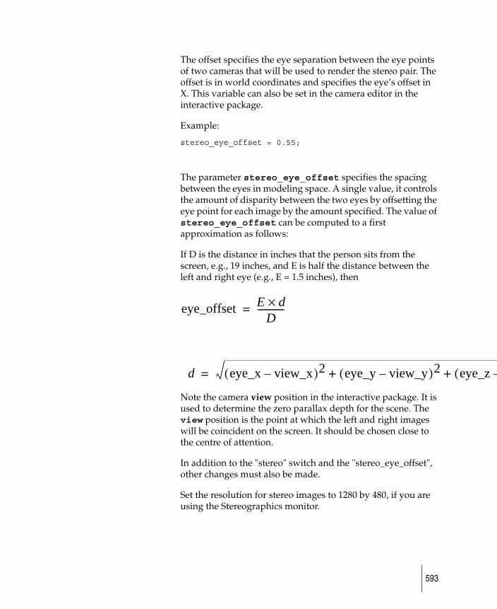
eye_z view_z–(
The offset specifies the eye separation between the eye points of two cameras that will be used to render the stereo pair. The offset is in world coordinates and specifies the eye’s offset in X. This variable can also be set in the camera editor in the interactive package.
Example:
stereo_eye_offset = 0.55;
The parameter stereo_eye_offset specifies the spacing between the eyes in modeling space. A single value, it controls the amount of disparity between the two eyes by offsetting the eye point for each image by the amount specified. The value of stereo_eye_offset can be computed to a first approximation as follows:
If D is the distance in inches that the person sits from the screen, e.g., 19 inches, and E is half the distance between the left and right eye (e.g., E = 1.5 inches), then
Note the camera view position in the interactive package. It is used to determine the zero parallax depth for the scene. The view position is the point at which the left and right images will be coincident on the screen. It should be chosen close to the centre of attention.
In addition to the "stereo" switch and the "stereo_eye_offset", other changes must also be made.
Set the resolution for stereo images to 1280 by 480, if you are using the Stereographics monitor.
eye_offset E d×D
------------=
d eye_x view_x–( )2 eye_y view_y–( )2+ +=
593
Good quality is necessary for stereo images. Ensure that the aalevel (both min and max) and aathreshold values are set appropriately.
The viewport for stereographic viewing should always be 0 1279 0 479. For the aspect, use 1280/1024 (the value will be computed).
The fov should be adjusted to the viewing distance between the user and the stereographic screen. In the attached example, set for a viewing distance of 19 inches, the fov = 2.0*atand(4.5/19.0).
If any lights of type ambient are used, ensure that the ambient_shade value is set to 0 (it defaults to 0.5) for each. If it is set to a value other than 0, the lighting will be different for each eye.
Render this SDL file once to create the pix files for both eyes.
Showing Stereo Images:
To view these files on the Stereographics monitor, use the stand alone program showstereo. If the pix files are not full screen resolution (1280 by 480), they will be resized to the correct resolution automatically, by pixel replication if they are too small, or by truncation if too large. If the image is too large, as much of the image as can fit on the screen will be shown, from the upper left corner.
Alternatively, you can use the standalone utility rb_stereo to create a red-blue stereo image that can be viewed on the monitor with readily-available red-blue “stereo” glasses.
Helpful Hints for Stereo Image Modeling
When creating images for stereo pairs, some effects work better than others. Keep the following in mind when creating your model:
594
1 Models that fit completely in the image window appear more three-dimensional than models that are cut off by the edges of the screen.
2 Thin, plain verticals are very difficult to merge into a single object when viewing, as there isn’t much information for the eye to use to combine them. Generally speaking, an object with a fair amount of detail (color and light variations, texture, irregularity in shape) provides more information than a plain object.
3 Very high contrast of lights and darks in the image results in ghost images.
4 The closer the viewpoint is to the back of the scene, the more the scene will project from the Stereographics display: the closer to the front, the more the scene will recede into the monitor. Remember that having objects too “close” to, or too “far” from the viewer’s eyes results in discomfort as the viewer crosses or uncrosses his or her eyes to merge the two images.
A useful example file is found in CourseWare/SDL/stereo.
595

596