SCREENING METHODOLOGY FOR NEEDS OF ROADWAY · SCREENING METHODOLOGY FOR NEEDS OF ROADWAY LIGHTING...

FINAL CONTRACT REPORT

SCREENING METHODOLOGY FOR NEEDS OF ROADWAY LIGHTING

JAMES H. LAMBERT, P.E. Associate Director

Center for Risk Management of Engineering Systems University of Virginia

Systems and

THOMAS C. TURLEY Graduate Student

Information Engineering University of Virginia

Department

Contract Research Virginia Transportation

Sponsored by Research Council

VIRGINIA

TRANSPORTATION RESEARCH COUNCIL

TRANSPORTATION RESEARCH COUNCIL

1. Report No. FHWA/VTRC 03-CR14

Standard Title Page- Report on Federally Funded Project 2. Government Accession No. 3. Recipient's Catalog No.

4. Title and Subtitle Screening Methodology for Needs of Roadway Lighting

7. Author(s) James H. Lambert, P.E., and Thomas C. Turley

9. Performing Organization and Address Center for Risk Management of Engineering Systems University of Virginia; P.O. Box 400747, 112 Olsson Hall Charlottesville, VA 22903

12. Sponsoring Agencies' Name and Address

FHWA P.O. Box 10249 Richmond, VA 23240

Virginia Department of Transportation 1401 E. Broad Street Richmond, VA 23219

5. Report Date June 2003

6. Performing Organization Code

8. Performing Organization Report No. VTRC 03-CR14

10. Work Unit No. (TRAIS)

11. Contract or Grant No. 60927

13. Type of Report and Period Covered Final

14. Sponsoring Agency Code

15. Supplementary Notes

16. Abstract Screening methods of AASHTO and NCHRP that assess the local potential for fixed roadway lighting to decrease nighttime crashes have not been updated since the 1970s. The methods dilute the influence of important factors, are inadequate for locations where crash histories are unavailable, and lack a traceable theoretical foundation. This report evolves and complements existing screening methods in order to develop an updated method to aid engineers and planners in the screening of needs for fixed roadway lighting. Development of the method adopts principles of risk assessment and management that have been previously applied in diverse disciplines. The existing screening methods, which provide a basis for the developed screening method, are strengthened by the development of a theoretical foundation in benefit-cost analysis. The developed method has two phases. In the first phase, an exposure assessment is developed to describe individual and population exposures to crashes. Needs are compared by night-to-day crash rates, measured directly or estimated indirectly, and traffic volumes. Outcomes of exposure assessment are identified based on potential crash reduction and costs of available lighting technologies. The second phase builds on selected concepts of the NCHRP method. In testing of the two-phase method, night crash histories for over eighty unlighted sections in three regions of Virginia are collected and studied. Example applications of the method to individual locations are demonstrated. The recommendations are as follows: (i) highway agencies should consider designating funds for lighting and visibility enhancement using the developed screening method in resource allocation; (ii) agencies should provide training and continuing education in the developed screening method, and emphasize the unity of principles of risk assessment and management across highway safety issues; (iii) through a testing phase, agencies should consider replacing the AASHTO and NCHRP methods with the developed method; (iv) agencies should perform regional data analysis and screening of unlighted locations on an annual basis; and (v) incorporate the method in holistic lighting master plans.

17 Key Words Roadway lighting, screening method, risk assessment, visibility

18. Distribution Statement No restrictions. This document is available to the public through NTIS, Springfield, VA 22161.

19. Security Classif. (of this report) Unclassified

20. Security Classif. (of this page) Unclassified

21. No. of Pages 70

22. Price

Form DOT F 1700.7 (8-72) Reproduction of completed page authorized



James H. Lambert, P.E. Associate Director


Thomas C. Turley Graduate Student

Systems and Information Engineering Department University of Virginia

Project Monitors Benjamin H. Cottrell, Virginia Transportation Research Council Wayne S. Ferguson, Virginia Transportation Research Council

Contract Research Sponsored by Virginia Department of Transportation

Virginia Transportation Research Council (A Cooperative Organization Sponsored Jointly by the

Virginia Department of Transportation and the University of Virginia)

Charlottesville, Virginia

June 2003 VTRC 03-CR14

NOTICE

The project that is the subject of this report was done under contract for the Virginia Department of Transportation, Virginia Transportation Research Council. The contents of this report reflect the views of the authors, who are responsible for the facts and the accuracy of the data presented herein. The contents do not necessarily reflect the official views or policies of the Virginia Department of Transportation, the Commonwealth Transportation Board, or the Federal Highway Administration. This report does not constitute a standard, specification, or regulation.

Each contract report is peer reviewed and accepted for publication by Research Council staff with expertise in related technical areas. Final editing and proofreading of the report are performed by the contractor.

Copyright 2003 by the Commonwealth of Virginia.

PROJECT TEAM

Center for Risk Management of Engineering Systems James Lambert Yacov Haimes Thomas Turley Della Dirickson Raynelle Deans Andrew Miller Jenny Murrill James Sanders Max Aronin

Raynelle Callender Amre Massoud Clare Patterson

Kenneth Peterson

Virginia Transportation Research Council Benjamin Cottrell Wayne Ferguson Michael Perfater

Virginia Department of Transportation Steve Brich

Travis Bridewell Pamela Brookes Chandra Clayton Butch Cubbage Mark Hodges

Ilona Kastenhofer Karen Rusak Jon Sayyar A1 Smith

Federal Highway Administration Carl Andersen

Acknowledgments

Others of the Virginia Department of Transportation (VDOT) and the Virginia Transportation Research Council (VTRC) who assisted in this project include: James Breeden, Jimmy Chu, Robert Feldman, Jim Gillespie, Jaroslaw Jastrzebski, Ralph Jones, Ray Khoury, Craig Manges, Robert Rasmussen, Timothy Rawls, and Llewellyn Slayton. Jim Havard of the Illumination Engineering Society and LITES, a lighting consulting business, also assisted.

iii

ABSTRACT

Screening methods of AASHTO and NCHRP that assess the local potential for fixed roadway lighting to decrease nighttime crashes have not been updated since the 1970s. The methods dilute the influence of important factors, are inadequate for locations where crash histories are unavailable, and lack a traceable theoretical foundation. This report develops and complements existing screening methods in order to provide an updated method to aid engineers and planners in the screening of needs for fixed roadway lighting. The method adopts principles of risk assessment and management that have been previously applied in diverse disciplines. The existing screening methods, which provide a basis for this method, are strengthened by the addition of a theoretical foundation in benefit-cost analysis. The method has two phases. First, an exposure assessment measures individual and population vulnerability to crashes. Needs are compared using night-to-day crash rates, measured directly or estimated indirectly, and traffic volumes. Outcomes of the exposure assessment are based on potential crash reduction and costs of available lighting technologies. In the second phase, a site-parameters assessment is developed to identify a set of engineering criteria that determines whether lighting would effectively reduce crashes. The developed site-parameters assessment is supported by extensive review of literature, classification of visibility-loss scenarios, and dialogue with engineers. The second phase builds on selected concepts of the NCHRP method. In testing the two-phase method, night crash histories for over eighty unlighted sections in three regions of Virginia were collected and studied, and the approach was applied to several locations. The recommendations are as follows: (i) highway agencies should consider designating funds for lighting and visibility enhancement using the developed screening method in resource allocation; (ii) agencies should provide training and continuing education in this method, and emphasize the unity of principles of risk assessment and management across highway safety issues; (iii) through a testing phase, agencies should consider replacing the AASHTO and NCHRP approaches with this one; (iv) agencies should perform regional data analysis and screening of unlighted locations on an annual basis; and (v) agencies should incorporate the new process in holistic lighting master plans. Future development of screening methods should identify when particular visibility-enhancing technologies•including fixed lighting, pavement markings, and remedies for veiling luminance•are uniquely effective.



James H. Lambert, P.E. Associate Director


Thomas C. Turley Graduate Student

Systems and Information Engineering Department University of Virginia

INTRODUCTION

Overview

Roadway lighting is an effective safety countermeasure against night crashes and for a general safety improvement along highways. Well-designed roadway lighting improves visibility, thereby enhancing nighttime driving conditions. However, a highway agency has limited resources and cannot completely and adequately address all needs with identical resources. A principle-based method of screening needs is useful to prioritize investigation of the needs for which installation of fixed lighting might be beneficial in terms of crash reduction. Other significant potential benefits of fixed roadway lighting, such as increased security and economic development, are not addressed by this review.

Review of Literature and Practice

Fixed roadway lighting is addressed by Wilken et al. (2001), Kramer (1999, 2001), ANSI (2000), Cottrell (2000), Edwards (2000), IES (2000), Walton (2000), Watson (2000), Gransberg (1998), Sandhu (1992), APWA (1986), and Janoff (1984, 1986). Traffic studies typically find that more than half of crash-related fatalities occur at night, during which time only one-fourth of the day's traffic is on the road. Nighttime conditions are associated with a fatality rate about three times higher than daytime. Fixed roadway lighting is one of the solutions to alleviate this discrepancy and reduce crashes. Several studies have quantified the crash-reduction factor provided by fixed roadway lighting. The International Commission on Illumination (CIE 1990) summarizes more than sixty crash studies from fifteen countries focused on the benefits of roadway lighting. Some 85% of the studies find that lighting is beneficial. Table 1 shows that the reduction of nighttime crashes was found to be between 9% and 75%. CIE (1990) concludes that "roadway lighting is successful; however, the installation of lighting cannot be expected to result in a reduction in crashes if there is a major non-visual problem at any particular site." Box

(1989) shows that lighting can reduce night crashes in a range of 20 to 36% and overall crashes at a rate of up to 14%. Griffith (1994) estimates a reduction of total property damage (TPD) crashes of 32%. Box (1972) shows that illumination could reduce night crashes by 40% on freeways. Crash reduction from lighting is further investigated by Dewar and Olson (2002), Trivedi (1988), Janoff (1984, 1986), and Marshall (1970).

Benefit-cost (B/C) analysis of lighting is addressed by IADOT (2001), NYMTC (2001), McFarland and Walton (2000), Janoff and McCunney (1979). Various agency practices in B/C analysis are summarized in Appendices A through D. The costs of fixed roadway lighting, which vary widely by design and by location, include: initial costs (construction), lifecycle costs (annual operation and maintenance costs), and work-force impacts that can result from new methods or guidelines. Candidate designs with varying associated costs include" arm-over- roadway, offset-on-pole, and high mast. Typical single high mast installation, e.g., eight 400- watt fixtures, can have an initial cost of over $100,000. The maintenance of all conventional and high mast equipment on approximately 1,000 poles in a region of central Virginia is approximately $450,000 per year. The cost of electricity for lights and signals in the same region is approximately $750,000 per year (Cottrell 2000). Fixed roadway lighting design and engineering are addressed by Staplin et al. (2001), Khan et al. (2000), Garber (2000), Couret (1999), Crawford (1999), Shaflik (1997), Jefferson (1994), FHWA (1993), and Janoff and Zlotnick (1985).

Table 1. Summary of the Benefits of Lighting (% reduction of nighttime crashes) (CIE 1990)

Road

Class

Urban Continuous

Pedestrian Crossings Rural Continuous

Junctions

Freeways Continuous

Interchanges

All crashes Sample Mean % studies

Range reduction

3 21 to 75 43 10 9 to 75 29

2 13 to 75 44 4 13 to 75 37

44 2 26 to 44 35

57 3 56 to 58 57

41

Crashes classification Pedestrians

Sample Mean % studies Range

reduction

2 46 to 75 51 4 16 to 57 42

64 8 32 to 74 54

Fatalities Sample Mean % studies Range

reduction

6 29 to 48 34 9 16 to 48 29

2 38 to 53 45 6 13 to 100 44

9

62

In practice, application of a lighting warrant typically precedes B/C analysis, since the latter involves more investigational resources. FHWA (1978) describes a lighting warrant as factual evidence of a proposed need, but notes that meeting a warrant does not obligate an agency to satisfy the need. Meeting of a warrant suggests that the proposed need be considered further in light of what resources are available, the traffic, the severity of hazards, and other

considerations. Screening (referred to by some practitioners as warranting) methods of the American Association of State Highway and Transportation Officials (AASHTO 1984, see Appendix E) and the National Cooperative Highway Research Program (NCHRP 1974, see Appendix F), have not been substantively revised since the 1970s, and thus fail to include thirty years of evolution of traffic volumes, automotive technology, roadway design, and public values concerning road safety. The AASHTO method emphasizes exposure variables, such as average daily traffic (ADT) and crash rate, but assigns arbitrary thresholds of concern for the variables. The NCHRP method adds emphasis to road geometry and operational parameters, but utilizes a scoring system whose basis is unclear and suspect. Neither method provides needed guidance for obtaining relevant crash rates for new or rebuilt roadways.

In summary, there is presently an opportunity for research that can provide a basis for a screening method for potential needs of fixed roadway lighting.

PURPOSE AND SCOPE

This study develops a screening method to establish priorities for locations that are identified as being in need of fixed roadway lighting installation or upgrade. The overall approach is to develop needed revisions to the two existing screening methods (AASHTO 1984, NCHRP 1974). With respect to either existing method or the current method, we prefer the term screening to that of the term warranting, because of misleading and imprecise implications that have accrued over the years to the latter term. Our effort aims for an objective process of applying quantitative and qualitative assessments of lighting needs. We address situations of new or totally reconstructed roads where there are partial or no data on existing travel conditions. We concentrate on fixed roadway lighting, but the principles in risk assessment and risk management of the developed method can be adapted to screen for other needs of visibility improvements. The effort does not address lighting design or particular lighting fixtures.

METHODOLOGY DEVELOPMENT

Overview

The purpose of this section is to describe the developed screening method of needs for roadway lighting. First we establish the context of the screening method. In succeeding subsections, we describe the development of the two major phases of the method: exposure assessment and site-parameters assessment.

A screening decision is based on outcomes of the two sequential phases" exposure assessment and site parameters assessment. Exposure assessment implements a streamlined benefit-cost analysis by relating night-to-day crash rates, traffic volume, and various exogenous variables. Site parameters assessment is performed by identifying a list of engineering

parameters that individually justify lighting as a beneficial method of visibility improvement for a specific section of road.

Figure 1 describes the context for the screening method within overall decision making for visibility improvement needs. The screening method originates with proposed needs, and it precedes the full investigation of potential needs. An aim of the screening method is to limit the number of needs going through full investigation. Potential lighting needs range from new construction and road alterations, to requests from localities to improve lighting. For example, a rural interstate may currently be unlighted but a newly constructed transit warehouse facility with a well lit parking area may cause veiling luminance problems prompting a request for the installation of fixed roadway lighting to alleviate the problem.

Screening Method

Evaluation

Funds Allocation

Proposed Needs

Accepted Projects

Rejected Projects

Figure 1. Funds Allocation Process for Visibility Enhancement Needs

Figure 2 describes that fixed roadway lighting is among other remedies that involve traffic control, which in turn are among other remedies for road-safety improvement.

Safety Improvements

Structures Roadway and roadside

Intersection and traffic control

Railroad-highway crossings

Fixed roadway lighting Traffic signals

Pavement markings and/or

delineators

High-mast fixtures

Continuous roadway fixtures

Figure 2. Fixed Roadway Lighting Among Other Traffic Safety Improvement Methods

Overview

Development of Exposure Assessment

Exposure assessment, the first phase of the screening method, consists of a streamlined benefit-to-cost analysis, based on the relationship established among a set of regional exogenous parameters, lighting costs, night-to-day crash rate ratio, and average daily traffic (ADT). First, the concept will be detailed. Second, a graphical interpretation to yield a screening decision for the exposure assessment will be demonstrated.

Method Development

Figure 3 is a graph that is useful to relate the hazard exposure, in terms of the average daily traffic exposed to the need, to the hazard severity, in terms of the night-to-day crash rate ratio. A need located in the bottom-left of the graph represents a low-exposure and low-severity condition. A need located in the top-fight of such a graph represents a high-exposure and high- severity condition, etc.

Low frequency High intensity

High frequency Low intensity

Average Daily Traffic

Figure 3. A Representation of the Risk Associated with Night Crashes

We proceed to develop a basis for the graph through application of benefit-cost analysis. A benefit-cost analysis for roadway lighting justification considers several variables to determine whether the benefits of lighting potentially exceed the costs. The benefit-to-cost ratio is defined to be the ratio of the expected cost of the night crashes avoided per mile per year and the cost of lighting per mile per year as follows"

Equation (1)" Benefit to Cost Ratio

365xADTx%N ADTx N/DxDCRxCRFx ACC 100,000,000 x (AIC + AMC + AEC)

where the variables ADT, %N_ADT, N/D, DCR, CRF, ACC, AIC, AMC, and AEC are as defined in Table 2.

Table 2. Benefit-to-Cost Analysis Variables for the Exposure Assessment Phase

Code Variable Unit ADT Average daily traffic vehicles per day %N_ADT Percentage of night traffic % of average daily traffic N/D Night-to-day crash rate ratio

DCR Day crash rate crashes per 10 VMT

CRF Crash reduction factor % of current crashes ACC Average crash cost $ per crash AIC Annualized installation cost of lighting $ per year per mile AMC Annual maintenance cost $ per year per mile AEC Annual energy cost $ per year per mile

An interval range of potential values for each of the exogenous variables, i.e., variables other than ADT (average daily traffic) and N/D (night-to-day crash rate ratio), is estimated. The ranges are set by consulting with experts from state transportation agencies, and by analyzing literature and field data. For example, the costs of crashes are addressed by Judycki (1994). Table 3 gives the ranges assigned to each variable. The ranges can be adjusted for any particular geographic region, environment, locality, or jurisdiction of interest. For example, a section of roadway serving a factory that has a night shift can have regularly more than one fourth of the overall traffic during nighttime. As well, the B/C ratio variable can be adjusted, intending either to pass more needs or to be more restrictive.

Table 3. Ranges of Exogenous Variables for the Exposure Assessment

Code Term Low High Unit B/C ratio •!• •:!• None

%N ADT DCR CRF ACC

Percentage of night traffic i•i•:••• N % of average daily traffic Day crash rate • • Crashes per 10 Crash reduction factor iiiiiiiiiiiii!!!•!•i•!!•i•iiiiiiiiiiii•ii•iiiiii•iii•iii!!! % of current crash Average crash cost

•:•i• •,i• $ per crash

AIC+AMC+AEC Cost of lighting per year per mile

Figure 4 shows the application of Equation (1), with the ranges of exogenous variables as stated in Table 3, to the screening of needs. For a benefit-to-cost ratio equal to 1.0, the extreme values of the interval calculation generate two curves separating three zones in the graph: (i) accepted, whose needs have exposure and severity such that the benefit-to-cost ratio exceeds 1.0 for all possible values of the exogenous variables, (ii) marginal, whose needs are such that the benefit-to-cost ratio exceeds 1.0 for some possible values of the exogenous variables, and (iii) rejected, whose needs are such that the benefit-to-cost ratio cannot exceed 1.0 for any possible values of the exogenous variables. Lighting needs can be plotted, such as at the cross, on such a graph, and their positions in terms of exposure (ADT) and severity (night-to-day crash-rate ratio) relative to the three zones yields the screening decision for the exposure-assessment phase.

Without a relevant crash history, it will be possible to use the indirect night-to-day crash rate ratio estimation method developed later in this report.

A streamlined benefit-cost analysis thus proceeds without a need for precise values of the exogenous variables. Consistent with principles of risk assessment, the graph contrasting severity and exposure makes it possible for users to grasp the priority of the need relative to the benefit-cost zones. Needs that are determined to be at least marginal at the exposure-assessment phase pass through to the next phase of site-specific parameters assessment, while others are rejected in this first phase of screening. Needs that are higher and farther fight on the graph may receive higher priority for further study, subject to a recognition of the uncertainty introduced into the B/C analysis by the exogenous variables. The exogenous-variable uncertainty leads to a wide or narrow swath of the 'marginal' region of the graph.

O

• 6.0-

• 5.0-

"=40-

• 3.0-

.= :2.0-

Z 1.0-

Accepted

• Current

Rejected ............................ Rejected -'", ....... •._..[...;....;..ll 10,000 100,000

Average Daily Traffic (vehicles per day)

Figure 4. Display That Assesses the Exposure of the Population Versus the Severity of Crashes

Overview

Development of Site-Parameters Assessment

An exposure assessment alone is not sufficient for a screening decision: A need that is justified by severity and exposure variables, as above, may have no feasible remedy in roadway

lighting. Thus this secondary phase of site-parameters assessment is developed to address whether lighting would potentially be effective. The site-parameters assessment develops a set of eight site-specific parameters that represent local design and engineering characteristics of the road section. Below, the development of a site-parameters assessment is described. Next the worksheet used to perform the site parameters assessment is shown and all parameters are described in structured narrative. Finally the steps to evaluate a need by the site-parameters assessment are described.

Method Development

The method development is as follows. The NCHRP (1974) screening method composed of four lists of twelve to twenty parameters is distilled to one unique list of eight parameters. The revision aims to diminish the dilution of low-weighted parameters from which the NCHRP method suffers. Some NCHRP parameters were combined, some were discarded, and some new parameters were added. For each parameter, a scale is developed, based on three thresholds corresponding to high, moderate, and low. Meeting the highthreshold in any single parameter indicates that installation of lighting would have some/possible/no benefit in terms of crash reduction. If a parameter on its own cannot provide sufficient evidence of lighting benefit, then no high threshold is defined. The approach simplifies the scoring method used by NCHRP (1974), which applied multiplicative weights (which themselves varied from parameter to parameter by as much as a multiplier of forty) to parameters which each had up to five thresholds. Table 4 defines the three thresholds for each of the eight parameters. The eight parameters of the new method are" section geometry, traffic mix, vehicle conflict opportunities, posted speed, curves and grades, veiling luminance, level of service, and intermodal transactions. The thresholds of the developed parameters were selected through discussion with experts, by referring to the literature, by referring to the existing NCHRP method, and by using a set of visibility-loss scenarios that are described in a later section of this report.

A description for each parameter follows. The structure of the description supports each site parameter as follows:

Rationale: Brief description of the parameter and intuition or modeling that suggests that visibility improvement would have some beneficial impact

Specific countermeasures." Does the parameter suggest that fixed roadway lighting or any available technology would be uniquely effective? Why is this parameter related to visibility and why can lighting improve the safety?

Each description provides a rationale for the high/moderate/low thresholds for the site parameter. Some number of parameters cannot score high. Those parameters did not provide enough evidence alone to indicate that lighting would have a benefit. For example, the level of service parameter cannot alone provide sufficient evidence that fixed roadway lighting would reduce nighttime crashes.

Table 4. Site Parameters Developed for the Second Phase of the Screening Method

Traffic mix

(percentage of qualified tracks in the overall traffic)

<15 % 15-25 % >25 %

Veiling Luminance

(percentage of luminous development frontage)

0-25 % 25-70 % 70-100 %

Curvature and grade Curvature Grade

<4 40_5 >5 Level- Rolling Mountainous No score

Lane configuration Lane width

Number of lanes

>10ft <10ft 6 or less lanes 6 or more lanes undivided divided

No score

Section/Intersection geometry Sight distance Median width Shoulder width

>400ft _<400ft 12-30ft <12ft >7fi _<7ft

Intersection/interchange <3/mile _>3/mile frequency

No score

Posted Speed <55 MPH _>55 MPH No score Level of Service D or better E or worse No score

Intermodal transactions

Distance to tourist, elderly venues and intermodal platforms Adjacent parking spaces

mile ½ mile No score

Prohibited both sides Permitted both sides No score

Site Parameter" Traffic Mix

Rationale: Traffic Mix

The prevalence of tracks in traffic increases the speed differential between vehicles thus increasing the likelihood of occurrence of crashes. Moreover, crash severity is higher when tracks are involved because of their higher weight relative to cars. Visibility decreases because of the size of the trucks, because smaller vehicles are unable to see around or over trucks and track drivers cannot see cars in their blind spots (Blower and Campbell 1998).

The traffic mix parameter accounts for the percentage of trucks in overall traffic mix. Traffic mix is considered to increase conflict opportunities, which may be addressed by improved lighting.

10

According to Blower and Campbell (1998), truck crashes at night tend to be more severe than during the day. They found a rate of 435 injuries per 1,000 crashes at night compared to 320 injuries per 1,000 crashes during the day. Moreover, the fatality rate per 1,000 crashes is three times higher at night than during the day (47 to 16) and the fatality rate per 1,000 injuries during the night is twice the day rate (108 to 51).

Specific Countermeasures" Traffic Mix

Countermeasures that have been explored in the laboratory include truck mirror design and video cameras on the sides and rear of the truck and cab displays to reduce blind spots. Roadway lighting is currently a cost-effective solution to increase visibility for both trucks and cars.

Site Parameter: Veiling Luminance

Rationale" Veiling Luminance

This parameter represents a combination of the volume of frontage development and the predominant type of development as characterized in the NCHRP forms. The parameter accounts for the light that floods unlighted roads from adjacent malls, and commercial and industrial areas.

This parameter accounts for the percentage of development frontage that produces disabling glare over the section of roadway considered. The presence of development can be associated with increased pedestrian activity and incoming/outgoing vehicles on the roadway, suggesting a synergy of the veiling luminance parameter with other parameters.

The volume of developed roadside frontage affects the number of vehicle movements in and out of the frontage areas. The location, rate of speed and identification of vehicles entering or leaving the roadway is of importance in the driving task.

Specific Countermeasures" Veiling Luminance

Lighting reduces the luminance ratio between the roadway ahead and the light coming from the side(s) of the roadway. Lighting can mitigate glare and increase sight distance around the vehicle.

11

Site Parameter: Curves and Grades

Rationale: Curves and Grades

The curve of a section of road is defined as the maximum curvature. The grade in a section of road is defined as the slope represented as a range of percentages associated with the classification "Level/Rolling/Mountainous."

• The maximum curvature affects the driver's ability to perceive road obstacles and anticipate changes in road geometry.

• The grade of the road alters the driver's perception of the road and speed regulation/braking ability.

Fitzpatrick et al. (2000) determined that as the radius of a curve decreases the likelihood that the driver will look to the inside of the curve increases, which would increase the amount of glare from oncoming traffic. Though headlights are designed to avoid such an interaction, the angle of approach in a curve changes the angle of light from the headlights into the lanes of oncoming traffic.

Curves in the road also affect the speed at which an intersection can be approached. Vehicles adjust their speed in order to remain in their respective lanes and accurately maneuver through the section of road. Grades on the road affect approach speed on a curve, whether it is excessive speed on a downgrade or slowing on an upgrade. Glennon (1987) produced the general conclusions that crash rates increase on grade road segments and with steepness. Weather conditions can have an adverse affect in relation to speed, grade, and curvature in the road as well, producing conditions where a vehicle may slide or spin if speed is not adjusted to accommodate.

Specific Countermeasures" Curves and Grades

At night, it becomes difficult to identify the direction of the road especially with factors such as curve and grade, oncoming traffic, and adverse weather. Lighting can play a role in identifying to the driver the presence of an upcoming curve and/or grade. Detection and identification stages are lengthened in driver perception-response time under nighttime conditions, and lighting allows the driver to make a quicker decision in response to the change in road geometry (Dewar and Olson, 2002). Lighting on a curve can also reduce the effect of glare from an oncoming car when maneuvering through the section of road. Roadway lighting increases the ability of the driver's eyesight to adjust to the oncoming direct light by minimizing the difference between that and the illumination on the road.

12

Site Parameter: Lane Configuration

Rationale: Lane Configuration

A greater number of lanes and decreasing lane width can contribute to vehicle conflict opportunities. The number and width of lanes causes drivers to focus inordinate attention on the positional level of driving tasks.

• This parameter constitutes a combination of number of lanes, lane width, left turn lane and channelization. It describes the operational complexity of a roadway section from the perspective of the driver.

• The developed scale is based on lane width and number-of-lanes metrics.

Both number of lanes and lane width are related to visibility. Greater visibility would keep drivers more aware and focused when driving in the tight, congested conditions created by a large number of lanes or small lane widths. As the lanes become narrower, tracking becomes more and more difficult for the driver who has to devote more attention to control steering in order to stay in the lane rather than performing other driving tasks. Therefore, it is important to improve visibility to facilitate the other driving tasks. As the number of lanes increases, the ability of the headlights to effectively light the periphery is greatly reduced, especially in inclement weather.

Site Parameter" Section/Intersection Geometry

Rationale: Section Geometry

This parameter specifically addresses the case of section and intersection geometry for urban roads or freeways. It emphasizes the constraints that a designer faces when the cost of ideal safety improvements are not supported by the budget. Geometrical or environmental conditions can lead to a non-optimal safety design, especially in the case of an old road. Modem design roles and improved construction techniques have eliminated this situation for many new

or recently altered roads.

• This parameter is a combination of four sub-parameters" sight distance, median width, shoulder width, and interchange or intersection frequency. It describes roadway geometry.

• The geometrical or environmental constraints related to a roadway can lead to non- optimal design for safety due to financial limitations.

Optimal sight distances are between 200 and 700 feet, depending on the speed and traffic conditions, according to NCHRP 1974.

The width of the median impacts drivers in the following ways: glare from headlights, distance between opposing traffic flows, and deceleration if a vehicle crosses the median. From 1994-1998, there were 267 cross-median crashes (CMC) on Pennsylvania interstates and

13

expressways, resulting in 55 deaths. Donnell et al. (2001) evaluated median safety in Pennsylvania, including the relationship between CMCs and median widths on interstates and expressways. Although they found that CMCs are rare events on Pennsylvania interstates and expressways, CMCs are an important safety concern because of their severity. Approximately 15% of CMCs involve fatalities and another 72% involve nonfatal injuries. By contrast, all crashes on the same road segments involve only 1% fatal and 52% nonfatal injuries. The use of a wide median is an excellent safety feature to eliminate potential interactions between opposing vehicles. A study by the North Carolina University Highway Safety Research Center linked crash rate with the median width (FHWA 1993). Statistical data from Illinois showed that by reducing an existing 64-foot median to 40-foot led to an increase of 23% in the total crash rate, while increasing a 40-foot median to 64-foot reduced the total crash rate by 18%.

In a review of safety aspects of two-lane roads (Garber 2000), an inverse relationship was found between crashes and shoulder width; crash rates tend to decrease as pavement width increases up to a width of about 25 feet.

Freeways are controlled-access facilities with interchanges rather than intersections. The lighting possibilities for these highways are either interchange lighting or continuous lighting. Griffith (1994) found that it is better to provide full lighting rather than interchange lighting on urban freeways. The night-to-day crash rate ratio was higher by 12% for the interchange lighting only. Theoretically, the illumination of a formerly unlighted urban freeway between interchange areas could reduce night crashes by 16%. Also, the night-to-day crash rate ratio for property- damage crashes is 32% higher for unlighted freeway sections than for fully lighted sections. Therefore, it appears that it is better to fully light a section of interstate rather than only the interchanges.

Another factor affecting the safety of freeways is that high interchange frequency impedes the design of acceleration and deceleration lanes and ramps. As a result, ramps can be steep and narrow, creating road hazards by increasing the quantity and magnitude of speed differentials among vehicles.

Specific Countermeasures" Section Geometry

Lighting can improve sight distance and counter-disabling glare from partially lighted intersections or interchanges. Leveling the amount of luminance on the entire section in place of alternating dark and illuminated areas represents an improvement for drivers, especially elderly drivers (Rumar 1998).

Site Parameter: Posted Speed

Rationale: Posted Speed

Visibility provided by headlamps is limited and can be less than the minimal stopping distance of the vehicle at the posted speed. High beams are designed to overcome this limit but

14

should not be used in the presence of other drivers. Speeding is particularly dangerous under night driving conditions because of the limited visibility offered by the headlights of the vehicle.

• The posted speed affects the stopping distance; as speed increases, more visibility is required for an effective stop.

• The severity of crashes increases with the differential of speed of the vehicles involved.

In order to reduce the likelihood of crashes, visibility improvement is an effective countermeasure. Moreover, reducing the likelihood of speed-related crashes has a direct benefit as high-speed crashes have severe consequences in terms of casualties, injuries and property damage. Ohta et al. (1991) found that the average time to detect speed changes at 50 mph was 2.06 seconds (for a following distance of 131 feet) versus 0.96 seconds at 30 mph (with a following distance of 66 feet). Evidence also shows that the perception of speed is different at night so that it is more difficult to develop correct estimates of speed. Improved visibility through lighting can help drivers perceive changes in relative distance more easily, and therefore, improve speed perception (Dewar & Olson 2002).

Specific Countermeasures" Posted Speed

Increasing illumination using fixed roadway lighting is arguably the best means to obtain visibility improvement for high-speed highways, especially extending the sight distance of drivers at night by overcoming the limitations of headlights.

Site Parameter" Level of Service

Rationale: Level of Service

Level of service involves assigning a letter grade (A, B, C, D, E, or F) to a roadway based on a conceptualized understanding of the roadway's traffic conditions (DOT BTS 1995). Level of service is often paired with ADT (average daily traffic) for a holistic understanding of traffic conditions of a roadway. The abstract nature of level of service is addressed by a characterizing guideline for each grade. A, for example, can be more specifically described as "free-flowing traffic"; C as "stable" traffic flow; and E as "extremely unstable." The way to measure the level of service is different for an intersection where cars may stop temporarily than for a continuous flow roadway. Furthermore, level of service may be variably dependent on peak versus off-peak times of day or year.

Level of service accounts for the delay and capacity-to-volume ratio Level of service is a continuum from A to F (choosing among A, B, C, D, E, or F). A represents very good traffic conditions and F represents very poor traffic conditions.

Traffic congestion and inadequate traffic flow are not only a nuisances for drivers, but also constitute unsafe driving conditions. With rapid changes in traffic flow, drivers are required to react quickly. Level of service refers not only to •traffic jams," but also addresses extremely

15

variable traffic flows caused by road geometry which makes drivers slow down and accelerate multiple times within a short period of time.

Specific Countermeasures: Level of Service

Brake lights were designed to warn other drivers in a traffic flow about reduced speed. However, with low visibility, brake lights lose their effectiveness. Lighting can improve the level of service by allowing drivers to see traffic flow rather than depending on brake light signals.

Site Parameter" Intermodal Transactions

Rationale: Intermodal Transactions

This parameter accounts for the inadequate driving behavior expected from tourists and elderly drivers who are unfamiliar with the area or vision-impaired (Hatch 1999, Rumar 1998). It also accounts for parking spaces that are located either along the road (parallel parking spots) or in a parking lot. The presence of parking spaces increases the number of vehicles slowing down to either parallel park or turn into a parking lot. All of these disruptions can increase the potential for a crash, especially at night when visibility is limited.

• Tourists and elderly drivers often display driving behaviors that are different from other drivers who have less attenuated vision or who are familiar with the section of roadway.

• The locations where tourists and elderly drivers are most likely to be driving at night include hospitals, night schools, tourist attractions, special events, and senior centers.

• The presence of parking lots leads to increased pedestrian activity and incoming/outgoing vehicles on the roadway.

• The presence of parallel parking spots may lead to more cars slowing down in the middle of the road.

• The presence of parking lots will lead to more cars braking from the traffic speed of the roadway as they turn into the lot.

This parameter measures the number of establishments or public services in relation to the road section. Buildings such as hospitals, night schools, senior citizen facilities, and popular night spots may attract a large number of drivers either unfamiliar with the road or who have limited night-driving abilities. The parameter considers intermodal platforms including airports, bus stations, bike paths, and other pedestrian-heavy areas. In order to obtain this data, the intersections or sections of roadway must be located on a local map detailing the presence of major facilities in the area and the distance to the facilities must be measured. Any of the applicable sites which fall within the 0.5-mile or 1-mile radii will determine the correct parameter for scoring purposes. Any kind of visibility improvement would assist unfamiliar or apprehensive drivers in reading signs, recognizing landmarks and tracking their lanes.

Parking lots also can increase the opportunities for crashes. The presence of parking spaces is a significant factor in road safety for drivers and pedestrians in urban areas.

16

Specific Countermeasures: Intermodal Transactions

Lighting can mitigate the visibility loss of elderly drivers and allow tourists to see further ahead to read signs and anticipate lane shifts. It can also improve the safety of vehicles traveling at night on roads with parking spaces. Lighting creates greater visibility so that drivers can see when another vehicle is attempting to park or turn into a parking lot.

Site Parameters Assessment Screening Decision

The user analyzes the need based on the eight parameters and places a check mark for each parameter in the appropriate column ("Low", "Moderate" or "High"). Then the user counts the number of "High," "Moderate" and "Low" check marks and enters the number in the appropriate cell at the bottom of the table ("Number of ratings").

For parameters comprised of two or three sub-parameters, there is a better chance to have at least a "Moderate" or "High." The highest result of the sub-parameters is used as the grade for the parameter. For example, the parameter would be "Low" if all its sub-parameters were rated "Low" but would be rated "Moderate" if at least one of its components were rated "Moderate."

Each parameter counts as one grade, even if it is a combination of sub-parameters. Thus, the sum of all the grades assigned must be equal to the number of parameters in the worksheet. If any one parameter cannot be assessed due to a lack of information, then the default is to grade it as "Low" for purposes of the count.

In order to allow room for flexibility, some parameters are not allowed to rate "High." For example, a need should not pass the site parameters filter only because of a high level of service. These "Low/Moderate" parameters need to be combined in a synergistic manner in order to pass the filter, for none of them is strong enough to justify lighting improvement.

Table 5 illustrates that the requirement for a need to pass the site-parameters assessment phase of the screening method is to score at least one "High" and/or four "Moderate." It is possible to set the thresholds for the decision making directly into the worksheet, in the computation sheet. These standards can be changed easily when required. It is possible to set the minimal number of "Moderate" rates to any value for it to pass as "Marginal." Needs scoring "Rejected" are left in the needs database for future consideration when data or other factors may propel the need into acceptance or simply discarded. Needs deemed "Accepted" move to the next evaluation stage and those deemed "Marginal" are given a lower priority. Therefore, "Marginal" needs are more dependent on the availability of resources committed to investigate them than "Accepted" needs for which a critical need has been identified.

Table 5. Evaluation Scores as a Basis for Decision in Site-Parameters Phase

Grade on scale Low Moderate High Result of the method Accepted N/A 4 or more or more Marginal N/A 2 or 3 0 Rejected N/A or 2 0

17

Combination of Exposure Assessment and Site-Parameters Assessment

The user now has both the exposure assessment and the site-parameters assessment for the section. Table 6 contains the possible combinations of results for phases of screening, and identifies the "Recommended decision" for the need.

Table 6. Combinations of Decisions of the Screening Method

Exposure Site parameters Recommended assess ment assess ment decision

Accepted Accepted Accepted Accepted Marginal Marginal Marginal Accepted Marginal Marginal Marginal Marginal Accepted Rejected Rejected Rejected Accepted Rejected Marginal Rej ected Rejected Rejected Marginal Rejected Rejected Reiected Reiected

Software Prototype Development

A prototype of software was developed for engineers and planners to screen needs for roadway lighting. The software is composed of four MS Excel worksheets, three of which display the overall results of the screening method, the exposure assessment, and the site- parameters assessment, and one for computations based on the user inputs.

The graphical user interface of the screening method software is as follows" Figure 5 gives the exposure-assessment worksheet. Figure 6 gives the site-parameters assessment worksheet. Figure 7 gives a summary of the results of the screening method. An example of a need identified as Rt. 434 is displayed. The characteristics of the example are fabricated and the site-parameters assessment worksheet is blank. For purposes of illustration, only the count of scores is filled in to display a result for the overall recommendation.

RESULTS

First, several studies of crash data that were developed in order to test the screening method are described. Then four examples applying developed screening method are given.

18

Study of Crash Data from Richmond District: Unlighted Nodes in Crash Record System

We studied a five-year dataset of all the recorded crashes in a region of Central Virginia (Richmond district) from January 1, 1997 through December 31,2001 (over 122,000 crashes). The crashes were related to nodes, i.e., intersections, landmarks or other milestones of the roadway formally described and stored in the Highway Traffic Records Inventory System (HTRIS) database.

The database we used included the following fields based on police reports:

• Document number • Route prefix, route number, and route suffix • Node, node offset • Crash date, crash hour • Severity (amount of property damage, injuries, deaths) • Crash lane, number of road lanes • Type of road facility or road structure

• Lighting situation • ADT (Average Daily Traffic on that stretch of roadway)

In order to evaluate the night-to-day crash rates from the data, we used the following formulas based on the standard assumption that 0.25 of total traffic occurs in the dark hours:

and

Similarly,

Thus,

Night to Day_ Crash Rate Ratio Night_ Crash_ Rate Day_Crash_Rate

Night_ Crash Rate Night_ Crashes Night_ Crashes Night_ADT 0.25 x Total_ADT

Day_Crash _Rate Day_Crashes Day_Crashes Day_ADT 0.75 x Total_ADT

Night to Day_ Crash Rate Ratio 3 x Night_ Crashes Day_Crashes

Equation 2

19

W

• XXX •e

• [] U •

•

[]

:o!le• a:• eJ q se• o •e:o-ol-1 q•!N

:o

o

o o

Figure 5. Screening Method Software: Exposure Assessment

20

o

i!I • A o

Z 0 o Z Z

Figure 6. Screening method software" site-parameters assessment

21

Name of need Rt. 434

Exposure assessment Site parameters assessment

Marginal Marginal

Recommended decision Marginal

Site parameters assessment 0 High 2 Moderate 6 Low

Exposure assessment

8.° l

o

• 6.0

,5.0

• 4.0

3.0

¢• 2.0 z

0.0 10,000

[] • •

x Rt. 434

100,000 Average Daily Traffic (vehicles per day)

Figure 7. Screening Method Software" Summary of Results

22

In order to find night-to-day crash rate ratios, we sorted the data by lighting condition. All crashes that occurred during the night, dusk, or dawn, were included in "night crashes," while all other crashes were included in "day crashes." In making this calculation, we discarded any crashes that did not have a "lighting situation" listed. In order to cover a variety of situations we elected to find the night-to-day crash rate ratios for the following queries for routes 250, 60, 1, and the entire dataset:

• <10,000 ADT, 2 lane road • <10,000 ADT, 4 lanes undivided • <10,000 ADT, 4 lanes or more divided • 10,000-20,000 ADT, 2 lane road • 10,000-20,000 ADT, 4 lanes undivided • 10,000-20,000 ADT, 4 lanes or more divided • >20,000 ADT, 2 lane road • >20,000 ADT, 4 lanes undivided • >20,000 ADT, 4 lanes or more divided

Tables 7 to 10 summarize the night-to-day crash rates ratios for the different queries.

Table 7. Summary of Night-to-Day Crash Rate Ratios in Richmond District

Entire Set Road Type ADT 2 lanes 4 lanes undivided 4 or more lanes divided

<10,000 1.89 1.42 1.40 10,000-20,000 1.38 1.36 1.21

>20,000 1.40 1.42 1.11

Table 8. Night-to-Day Crash Rate Ratios on Rt. 1 in Richmond District

Route 1 Road Type ADT 2 lanes 4 lanes undivided 4 or more lanes divided

<10,000 1.79 1.01 1.57 10,000-20,000 1.60 1.05 1.47

>20,000 N/A 1.09 1.22



<10,000 2.25 1.82 3.01 10,000-20,000 1.78 1.02 2.31

>20,000 0.33 1.15 0.93

23



<10,000 1.50 1.12 1.08 10,000-20,000 1.90 0.99 1.17

>20,000 N/A N/A 1.30

In reviewing the total crash database in Richmond district from January 1, 1997, through December 31, 2001, we elected to identify nodes with a high number of crashes. We were able to identify nodes with lighting problems by analyzing the types of crashes that occurred on these nodes (i.e., crashes that occurred at night with lighted or unlighted conditions). With this data, we calculated the night-to-day crash ratios for the roadway in the vicinity of the node.

The initial step was the identification of the nodes with the highest number of total crashes without regard to the lighting situation data. We discarded crashes that did not have node numbers assigned in the database. The discarded crashes included entries with "999999" in the Node field, or entries where the Node field was left blank, indicating that the node number for the crash was not entered into the database. We discarded crashes where there was no recorded AADT or where the AADT was entered as "0" and discarded crashes on interstates. The above steps left us with 63,649 crashes to analyze. We sorted the nodes by number of crashes and concentrated on the 60 nodes with the greatest number of crashes.

For those nodes, we decided on a number of fields to focus on in order to obtain useful data for our analysis. These fields included: total crashes, day crashes, night crashes, lighting situation, node offset maximum, and node offset mean. With a number of the crashes we could determine the night-to-day crash rate ratios for nodes that had a majority of unlighted crashes so we could assume that these nodes were primarily unlighted. Also in collecting our crash data we made the assumption that any crashes that occurred during "dawn" and "dusk" conditions would be considered nighttime. Finally, in the lighting section, there were a few nodes with "not stated" for the lighting field. The database included the time of day when the crash occurred, so we assumed that any crash occurring between 8AM and 8PM would be considered daytime, and anything else would be considered unlighted. Although this assumption of night or day classification does not account for seasonal changes and daylight savings time, it does place the majority of night crashes into the proper category.

To obtain the night-to-day crash ratios for each node, we had to decide which nodes we wanted to include in our analysis. We identified nodes that had primarily unlighted crashes. However, there were very few nodes that were totally one type of crash (lighted or unlighted). We decided that nodes with 2/3 more crashes on unlit sections should be considered unlit nodes. Table 11 shows that out of the 60 nodes with greatest number of crashes, 37 had two-third of unlighted night crashes. The maximum crash rate was 2.68 out of these nodes, the mean was 1.07. There were relatively very few pedestrian injuries recorded in the database, with 4 pedestrian injuries being the highest of any of the nodes. There were 574 pedestrian injuries out of the 63,649 crashes. For pedestrian fatalities, the statistics were smaller, with one node having

24

a fatality. There were 57 pedestrian fatalities. Figure 8 shows the result of the above study in terms of nodes on a plot of ADT vs. night-to-day crash rate.

Table 11. Crash Data Grouped by Nodes in Richmond District

Night- Night- N/D Total Day Lighted Unlighted Ped. Ped. Ratio AADT Crashes Crashes Crashes Crashes Injury Fatality 2.68 23,000 106 56 5 45 0 0 1.26 29,000 126 88 11 26 0 1.59 38,000 124 81 9 34 0 0 1.56 34,000 121 79 12 29 0 1.37 35,000 121 83 10 28 0 0 1.57 34,000 103 67 10 25 0 1.24 50,000 114 80 9 24 0 1.52 14,000 95 63 4 28 0 0 1.48 13,000 105 69 5 29 1.48 64,000 97 65 31 0 0 1.45 24,000 87 58 4 24 0 1.38 42,000 94 63 6 23 2 0 1.03 47,000 102 76 3 23 0 0 1.28 35,000 98 68 9 20 0 1.06 56,000 135 99 9 26 0 1.18 20,000 85 61 2 22 0 0 0.86 13,000 140 108 4 27 0 0.92 33,000 102 78 4 20 0 0 0.95 33,000 163 123 13 26 0 1.06 3,900 88 65 0 23 0 0 0.97 35,000 102 77 2 23 0 0 0.74 29,000 127 102 8 17 0 0 1.00 23,000 99 72 3 21 3 0 1.00 21,000 87 63 7 14 3 0 0.70 37,000 101 82 5 14 0 0 0.89 29,000 83 64 5 14 0 0 0.88 19,000 89 68 4 16 0 0.59 53,000 99 82 5 11 0 0.80 35,000 91 71 6 13 0 0.56 28,000 101 85 0 16 0 0 0.77 70,000 88 70 6 12 0 0 0.45 51,000 108 94 13 0 0 0.45 70,000 100 87 4 9 0 0 0.59 29,000 92 76 2 13 0 0.58 37,000 89 73 4 10 2 0 0.57 51,000 95 79 3 12 0

25

2.5

2.0

1.5

1,0

0.5

0.0 iO,O00 100,000


Figure 8. Summary of the Night-to-Day Crash Rates Ratio Collected for Nodes in Richmond District

Study of Crash Data: Unlighted Two-Mile Sections

Next, we performed a study of night-to-day crash-rate ratios on a selection of two-mile sections of unlighted road in a six-year period between January 1, 1996 and December 31,2001. The sections were selected from three regions" Tidewater Virginia, Central Virginia, and Northern Virginia. The selected sections were stratified by average daily traffic, posted speed and lane configuration. We collected the number of crashes under each for daytime conditions and nighttime conditions, extracting the totals for each of property-damage-only, injury, and fatal crashes. In addition, we collected the average daily traffic for each section. Next, we adopted the typical assumption that 3/4 of daily traffic occurs in daytime conditions and 1/4 under nighttime conditions; the assumption was vetted with engineers and planners of the system under investigation. We processed the data to obtain the night-to-day crash rate ratios.

VDOT provided us with a list of unlighted roads in Richmond district (coded 'R'), Hampton Roads district (coded 'H') and Northern Virginia district (coded 'N') that are divided into groups based on their average daily traffic volume (ADT), posted speed and lane configuration. We collected crash data on two-mile sections for every road. Tables 12 to 21 provide the geographic locations of the sections of road we studied. The "X node" means the beginning node, and "Y node" means the ending node of the section considered.

26

Posted Speed 55 mph

Table 12. Richmond District: Roads With <10,000 ADT, Posted Speed 55 mph and Either 2 Lanes or 4 Lanes (undivided)

<10,000 ADT 2 lanes

ID Route County X node R1 Rt. 54 Hanover Rt. 671 R2 Rt. 522 Powahatan Goochland Co. Line R3 Rt. 249 New Kent Rt. 155

4 lane divided

Y node mi. east of Rt. 671

Rt. 711 Rt. 106

R4 Rt. 360 Nottoway Rt. 49 R5 Rt. 460 Dinwiddie Rt. 627 R6 Rt. 60 New Kent Rt. 106

Amelia Co. Line Rt. 628

mi. east of Rt. 106

Posted Speed 45 mph

Table 13. Richmond District: Roads With 10,000- 20,000 ADT, Posted Speed 45 mph and Either 2 Lanes or 4 Lanes (undivided)

10,000 20,000 ADT 2 lanes

ID Route County X node R7 Rt. 167 Henrico Quioccasin Road R8 Rt. 144 Chesterfield Rt.

4 lane undivided

Y node Three Chopt Road mi. north of Rt.

R9 Rt. Chesterfield Rt. 144 R10 Rt. 460 Prince George Rt. 629 R11 Rt. 460 Prince George 0.44 mi. east of Rt. 625

Rt. 620 mi. east of Rt. 629

0.28 mi. west of Rt. 618

Posted Speed 55 mph

Table 14. Richmond District: Roads With 10,000 20,000 ADT, Posted Speed 55 mph and 4 Lanes (either divided or undivided)

10,000 20,000 ADT 4 lanes undivided

ID Route County X node R12 Rt. 460 Prince George Sussex Co. Line R13 Rt. 460 Prince George Rt. 156

4 lane divided

Y node mile west of line

mi. east of Rt. 156

R14 Rt. 156 Henrico 1-295 R 15 Rt. 60 New Kent Rt. 106 R16 Rt. 301 Hanover Rt. 640

mi. south of 1-295 mi. west of Rt. 106

Rt. 643

27

Posted Speed 45 mph

Table 15. Richmond District: Roads With 20,000 ADT, Posted Speed 45 mph and 4 Lanes (divided)

>20,000 ADT 4 lanes divided

ID Route County X node R17 Rt. 360 Chesterfield Rt. 288 R18 Rt. 33 Henrico Parham Road R19 Rt. 360 Hanover Rt. 770

Y node Rt. 653

Bremner Blvd. mi. east of Rt. 770

Table 16. Northern Virginia District: Roads With 10,000 ADT

Posted Speed 45 mph

55 mph

<10,000 ADT 2 lanes

ID Route X Node Y Node N1 Rt. 600 Rt. 242 Rt. 1014 N2 Rt. 645 Rt. 29 Rt. 3546 N3 Rt. 15 Prince Wm Line Thoroughfare

4 lane divided N5 Rt. 29 Rt. 845 Rt. 665

2 lanes N4 Rt. 611 Rt. 50 Rt. 744

Table 17. Northern Virginia District: Roads With 10,000- 20,000 ADT

Posted Speed 45 mph

55 mph

10,000 20,000 ADT 4 lane undivided

ID Route X Node Y Node N7 Wiehle Ave Rt. 675 Rt. 606

2 lane N6 Rt. 9 Rt. 689 Hillsboro

Table 18. Northern Virginia District: Roads With 20,000 ADT

Posted Speed 45 mph

55 mph


ID Route X Node Y Node N8 Rt. 7 Cascades Pkwy Loudoun Line N9 Rt. 236 Rt. 661 Rt. 649 N10 Rt. 50 Rt. 657 Rt. 7100 N11 Baron Cameron Rt. 6656 Rt. 7 N 12 Rt. 7 Rt. 1795 N 13 Rt. 28 Fairfax Line

Loudoun Line Rt. 1039

28

Posted Speed

55 mph

Table 19. Hampton Roads District: Roads With 10,000 ADT

<10,000 ADT

2 lanes

H1

Route X node Y node

Rt. 32 NC line Rt. 642

Isle of Wight Co. H2 Rt. 10 line Rt. 125

H3 Rt. 30 1-64 Rt. 60

Table 20. Hampton Roads District: Roads With 10,000 20,000 ADT

Posted Speed

45 mph

55 mph

10,000 20,000 ADT 2 lanes

H4

H5

Route X node Y node

Rt. 5 Rt. 199 Rt. 5000

Rt. 125 Rt. 622 Rt. 628

4 lane undivided

H6 Rt. 460 Rt. 58 Rt. 634

H7 Rt. 460 Rt. 258 Rt. 636

H11 Rt. 460 Rt. 258 Rt. 620

4 lane divided

H8 Rt. 17 Rt. 258 Rt. 620

Rt. 58 Suffolk H9 Bypass Rt. 460 Rt. 13, 32, Bus.

H10 Rt. 58 Greensville,

Southampton Co. Line

Rt. 35

Posted Speed

45 mph

Table 21. Hampton Roads District: Roads with 10,000 ADT


H12

H13

Route

Rt. 199

Rt. 60

X node

Rt. 615

Rt. 199

Y node

Rt. 612

Rt. 607

29

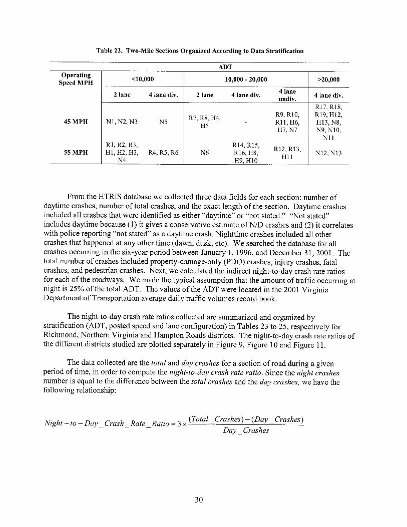
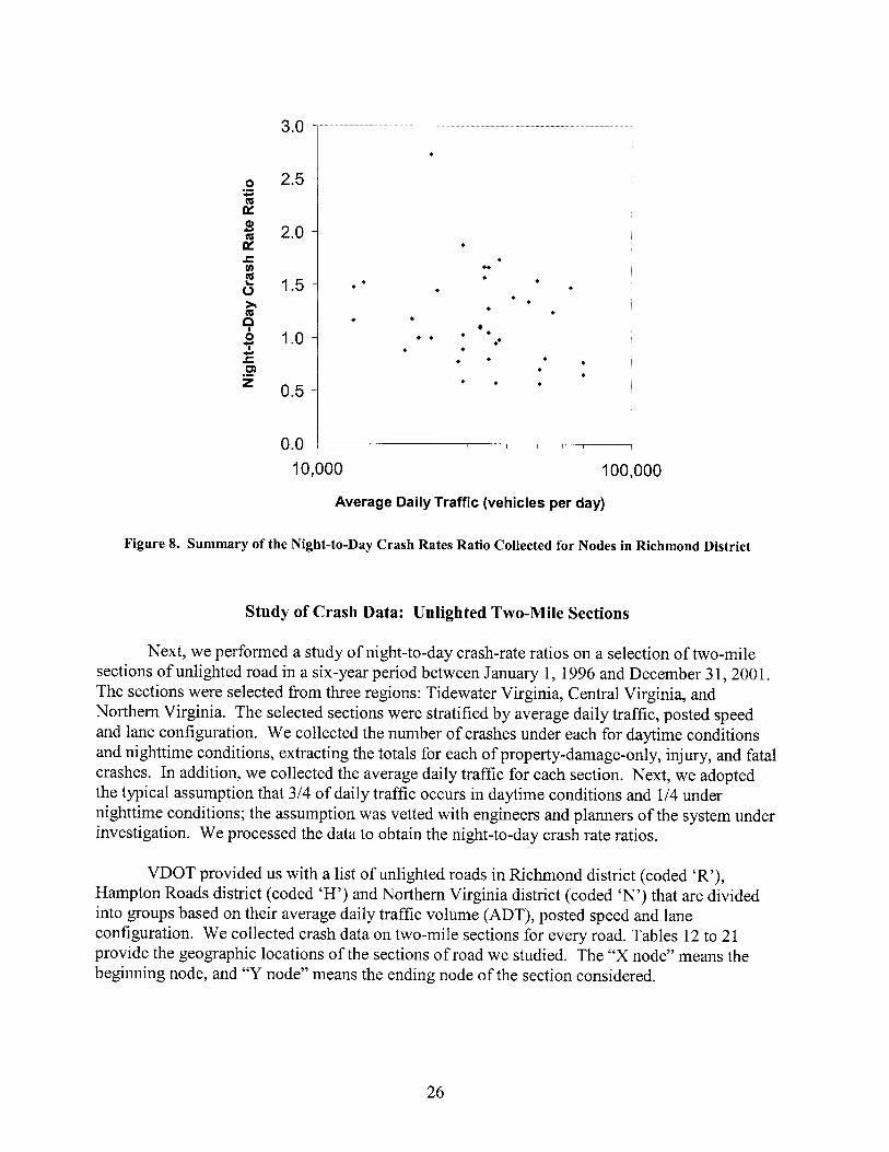
Table 22. Two-Mile Sections Organized According to Data Stratification

ADT Operating Speed MPH

45 MPH

55 MPH

<10,000

2 lane

N 1, N2, N3

R1, R2, R3, H1, H2, H3,

N4

4 lane div.

N5

R4, R5, R6

10,000 20,000

4 lane 2 lane 4 lane div. undiv.

R7, R8, H4, H5

R9, R10, Rll, H6, H7, N7

R14, R15, N6 R16, H8, R12, R13,

Hll H9, H10

>20,000

4 lane div.

R17, R18, R19, H12, H13, N8, N9, N10,

Nll

N12, N13

From the HTRIS database we collected three data fields for each section: number of daytime crashes, number of total crashes, and the exact length of the section. Daytime crashes included all crashes that were identified as either "daytime" or "not stated." "Not stated" includes daytime because (1) it gives a conservative estimate of N/D crashes and (2) it correlates with police reporting "not stated" as a daytime crash. Nighttime crashes included all other crashes that happened at any other time (dawn, dusk, etc). We searched the database for all crashes occurring in the six-year period between January 1, 1996, and December 31,2001. The total number of crashes included property-damage-only (PDO) crashes, injury crashes, fatal crashes, and pedestrian crashes. Next, we calculated the indirect night-to-day crash rate ratios for each of the roadways. We made the typical assumption that the amount of traffic occurring at night is 25% of the total ADT. The values of the ADT were located in the 2001 Virginia Department of Transportation average daily traffic volumes record book.

The night-to-day crash rate ratios collected are summarized and organized by stratification (ADT, posted speed and lane configuration) in Tables 23 to 25, respectively for Richmond, Northern Virginia and Hampton Roads districts. The night-to-day crash rate ratios of the different districts studied are plotted separately in Figure 9, Figure 10 and Figure 11.

The data collected are the total and day crashes for a section of road during a given period of time, in order to compute the night-to-day crash rate ratio. Since the night crashes number is equal to the difference between the total crashes and the day crashes, we have the following relationship:

Night- to Day_ Crash Rate Ratio 3 x

(Total Crashes) (Day Crashes) Day_Crashes

30

Table 23. Richmond District: Night-to-Day Crash Rate Ratios Organized According to Data Stratification

ADT

Operating Speed MPH

45 MPH

55 MPH

<10,000 10,000-20,000 >20,000

2 lane 4 lane div. 2 lane 4 lane div. 4 lane undiv. 4 lane div.

1.33, 2.33, 1.93, 1.11, 1.52, 1.06 1.23 2.23

0.25, 0.50, 1.50, 0.79, 2.01, 3.21, 1.00, 1.20 3.00 3.50 2.40

Table 24. Northern Virginia District: Night-to-Day Crash Rate Ratios Organized According to Data Stratification

ADT

Operating Speed MPH

45 MPH

55 MPH

<10,000 10,000-20,000 >20,000


10.32, 1.09, 1.67 3.32 1.50, 2.02,

1.33 2.09, 2.28

0.25 1.86 1.25, 1.43

Table 25. Hampton Roads District: Night-to-Day Crash Rate Ratios Organized According to Data Stratification

ADT

Operating Speed MPH

45 MPH

55 MPH

<10,000 10,000 20,000 >20,000


0.38, 1.74 1.40, 1.35 1.80, 1.08

1.83, 1.65, 1.24 1.01, 1.48, 2.16 1.85

The results produced by the HTRIS queries reveal a range of indirect night-to-day crash ratios between 0.25 and 10.32. The smallest reported crash ratios appear at an ADT of less than 10,000 (0.500 for 2-lane, and 0.789 for 4-lane divided road sections). A trend is that lower crash rates are associated with lower ADTs. Although this seems intuitively correct, it may not be strong enough based on the above data, to classify as a trend. However, some of the highest crash

31

rates are found at the higher speed stratification (3.0 and 3.5 at 55 MPH). This relationship indicates that a combination of more lanes, and higher ADTs would lead to the highest crash ratios, though currently there are no data points in these stratifications. Figures 6 to 8 give the scatter plots of night-to-day crash rate ratios versus ADT, with ADT represented in a logarithmic scale.

Indirect Estimation of Night-to-Day Crash Rate Ratio

An ancillary purpose of the two-mile sections study is to be able to predict potential crash ratios for roadways where crash data is not available, such as for new or altered roads. For roads where crash data is not available, the stratification of the road can be compared to those provided in Table 26. The average night-to-day crash rate ratio for that stratification can then be assumed for the corresponding roadway with no data.

Table 26. Indirect Night-to-Day Crash Rate Ratio Estimation Table

ADT

Operating Speed MPH

45 MPH

55 MPH

<10,000 10,000-20,000 >20,000

4 lane 2 lane 4 lane div. 2 lane 4 lane div. 4 lane div. undiv.

1.33, 1.09, 1.67

0.38, 1.06, 10.32 1.52, 1.74

0.25, 0.50, 1.01 1.48, 1.24, 1.65, 0.79, 1.50,

3.50 1.86 1.85,2.01, 1.83, 3.00 2.40, 3.21

1.23, 1.33, 1.35, 1.40, 2.33, 3.32

1.08, 1.11, 1.50, 1.80, 1.93, 2.02, 2.09, 2.23,

2.28

1.00, 1.20, 1.25, 1.43 2.16

In this effort we seek to predict the night-to-day crash rate ratio of a section of road knowing only its characteristics or stratification variables of the indirect night-to-day crash rate ratio estimation from Table 26. This indirect evaluation is then used in the exposure assessment phase of the screening method. In order to account for the uncertainty introduced by this indirect estimation, the values of the "indirect night-to-day crash rate ratio" table can be rescaled by a coefficient. For example, on average, two lane roads with a posted speed below 45 MPH and an ADT below 10,000 were found to have a Night-to-Day crash rate ratio of 1.25, therefore, the value used in the screening method for such a roadway considered is 1.25 x 0.50 0.63. Based on the AASHTO warranting method, a value of 0.50 would represent our most defensible value. In its warrants, AASHTO compares the Night-to-Day crash rate ratio of the considered roadway to the average on similar sections. The threshold value to pass the screening method is 2.0, which leads to our recommendation of the scaling factor of 0.50 stated above (AASHTO 1984).

32

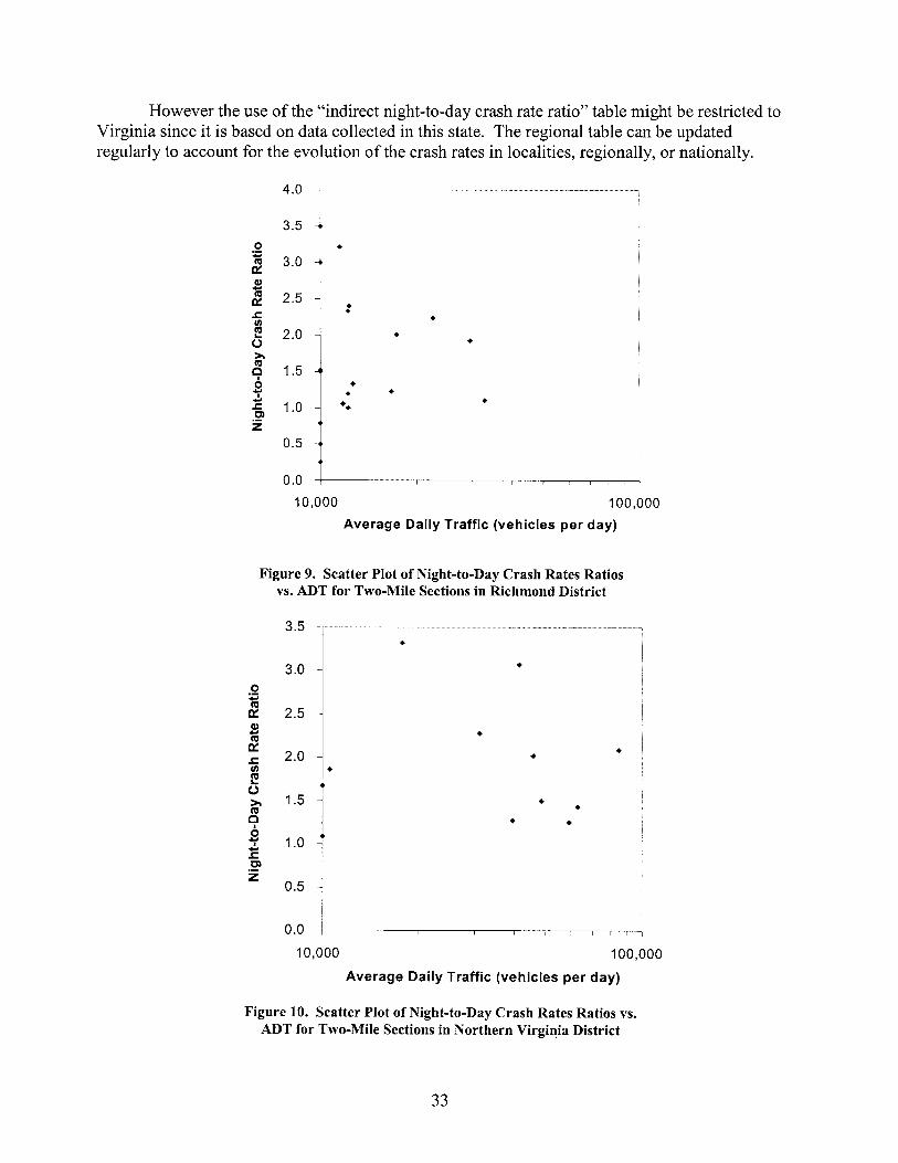
However the use of the "indirect night-to-day crash rate ratio" table might be restricted to Virginia since it is based on data collected in this state. The regional table can be updated regularly to account for the evolution of the crash rates in localities, regionally, or nationally.

100,000 Average Daily Traffic (vehicles per day)

Figure 9. Scatter Plot of Night-to-Day Crash Rates Ratios vs. ADT for Two-Mile Sections in Richmond District

3.0

1.5

1.0 -'

0.5

0.0

10,000 100,000 Average Daily Traffic (vehicles per day)

Figure 10. Scatter Plot of Night-to-Day Crash Rates Ratios vs. ADT for Two-Mile Sections in Northern Virgin, ia District

33

.£ 2.0

IZ 1.5

m 1.0

0

• 0.5-

0.0

10,000 100,000


Figure 11. Scatter Plot of Night-to-Day Crash Rates Ratios vs. ADT for Two-Mile Sections in Hampton Roads District

Integration of Two-Mile Sections Study With Unlighted Nodes Study

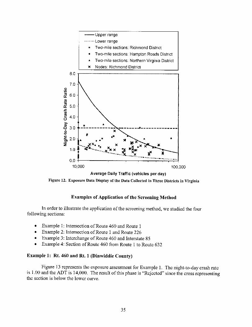
Figure 12 shows the scatter plots of the datasets collected in three districts in Virginia: Richmond, Northern Virginia and Hampton Roads districts. The dataset called "nodes" summarizes the data collected in the report section named Unlighted nodes in crash record system "Study of crash data: Unlighted nodes from Richmond district." The datasets called by a district name summarize the section named "Study of crash data: Unlighted two-mile sections." Needs are displayed on the exposure assessment chart of the screening method, so that a particular need can be compared to a regional set of need. A need out of the cluster of other needs can be subject to further investigation.

34

Upper range Lower range

[] Two-mi=,ie •sections* Richmond District

• Two-mile sections Hampton Roads District

• Two-mile •se.ctions Northern •Vi•rginia District

x Nodes: Richmond District

Average Daily Traffic (vehicles per day) Figure 12. Exposure Data Display of the Data Collected in Three Districts in Virginia

Examples of Application of the Screening Method

In order to illustrate the application of the screening method, we studied the four following sections:

• Example 1" Intersection of Route 460 and Route 1 • Example 2: Intersection of Route 1 and Route 226 • Example 3: Interchange of Route 460 and Interstate 85 • Example 4: Section of Route 460 from Route 1 to Route 632

Example 1- Rt. 460 and Rt. 1 (Dinwiddie County)

Figure 13 represents the exposure assessment for Example 1. The night-to-day crash rate is 1.00 and the ADT is 14,000. The result of this phase is "Rejected" since the cross representing the section is below the lower curve.

35

8/0

7,¸0

• 5.0

4.0

6 3.0

• 2.O

1.0 bum,m

m..q

0.0 10.,•00!0 100• 000

Average Daily Traffic (vehicles per day) Figure 1_3. Exposure Assessment Display for Example 1_" Rt. 460 and Rt. 1_

Table 27 represents the site parameters assessment worksheet for Example 1. Based on the thresholds described earlier, the result for the site parameters assessment is "Marginal," since only two "Moderate" are checked.

The end result of Example 1 is "Rejected," since the result of the exposure assessment is "Rejected" and the result of the site parameters assessment is "Marginal."

36

Table 27. Site Parameters Assessment Worksheet for Example 1" Rt. 460 and Rt. 1

Traffic mix

(percentage of qualified trucks in <15% the overall traffic) Veiling luminance


0-25%

15-25% >25%

25-70% 70-100%

Curvature and grade Curvature

Grade <4

Level- Rolling 40_50 >5

Mountainous No score


Number of lanes

>10ft

6 or less lanes undivided

SOft

6 or more lanes divided

No score

Section/intersection geometry Sight distance Median width Shoulder width

Intersection/interchange frequency

>400fi _<400fi 12-30fi <12ft >7ft _<7fi

<3/mile _>3/mile

No score

Posted speed Level of service



<55 MPH

D or better _>55 MPH No score

E or worse No score

mile ½ mile

Prohibited both sides Permitted both sides

No score

No score

Example 2" Rt. 1 and Rt. 226

Figure 14 represents the exposure assessment for Example 2. The night-to-day crash rate is 0.40 and the ADT is 4,900. For an ADT below 10,000 the need cannot be represented directly on the graph, so the ADT is set to 10,000. In this case, the result is "Rejected."

37

0.0 O, 000

Rt. and Rt. 2:26 ...........

...............

100• 000 A•ve•rage Daily Traffic (vehicles per •day)

Figure 14. Exposure Assessment Display for Example 2" Rt. 1 and Rt. 226



Example 3" Rt. 460 and 1-85

Figure 15 represents the exposure assessment for Example 3. The night-to-day crash rate is 1.00 and the ADT is 45,000. The result is "Marginal" since the need is located between the curves.


The end result of Example 3 is "Marginal," since the result of the exposure assessment is "Marginal" and the result of the site parameters assessment is "Marginal."

38

Table 28. Site Parameters Assessment Worksheet for Example 2: Rt. 1 and Rt. 226

Traffic mix

(percentage of qualified trucks in the overall traffic) Veiling luminance


<15%

0-25 %

15-25% >25%

25-70 % 70-100 %


Grade <4°

Level- Rolling 4°-5° >5°



Number of lanes

>10ft


•lOfl


No score



>40Oft •OOft

12-3Oft <12ft >7fl •ft

<3/mile •/mile

No score

Posted speed Level of service

<55 MPH

D or better •5 MPH No score

E or worse No score



mile ½ mile No score

Prohibited both sides Permitted both sides No score

39

8.¸0

7.¸0

.£ 6.0

• 5.0

4.0

6 3.0

• 2.0

Rt. 46,0 and 1-85

4'm4" enmq t4mamqmm'bbt4

t'mmmq O.•O

I O, 000 00,000 Average Daily Traffic (vehicles per day)

Figure 15. Exposure Assessment Display for Example 3: Rt. 460 and 1-85

Table 29. Site Parameters Assessment Worksheet for Example 3: Rt. 460 and 1-85

Traffic mix

(percentage of qualified trucks in <15% 15-25% the overall traffic) Veiling luminance


0-25% 25-70%

>25%

70-100%


Grade <4°

Level- Rolling 40_5 >5



Number of lanes

>10Ut


_<lOft


No score



>40Oft

12-3Oft >Tfl

<3/mile

_<40Oft

_<12fl _<7fl

>_3/mile

No score

40

Posted speed <55 MPH >_55 MPH No score

Level of service D or better E or worse No score


Distance to tourist, elderly venues mile ½ mile No score and intermodal platforms Adjacent parking spaces Prohibited both sides Permitted both sides No score

Example 4" Rt. 460 between Rt. 1 and Rt. 632

Figure 16 represents the exposure assessment for Example 4. The night-to-day crash rate is 0.33 and the ADT is 14,000. The result is "Rejected".

8.0

7.0

1.0

0.0

Rt. 460 bet"ween Rt. and Rt. 632

:1 O, O00i 00,000 Ave:rage Daily Traffic (vehicles per day)

Figure 16. Exposure Assessment Display for Example 4: Rt. 460 Between Rt. 1 and Rt. 632


41


As a summary of the results of the four case studies, the end results are displayed. The original NCHRP score and the relevant threshold to pass the warrant is added under each table of results to assess the consistency of the screening method in comparison to the former NCHRP warranting method.

Figure 17 displays all four examples. Only one passes the exposure assessment phase of the screening method, all the others are rejected, for the particular settings of the exogenous variables.

Table 30. Site Parameters Assessment Worksheet for Example 4" Rt. 460 Between Rt. 1 and Rt. 632

Traffic mix

(percentage of qualified trucks in <15% 15-25% >25% the overall traffic) Veiling luminance


0-25% 25-70% 70-100%

Curvature and grade Curvature Grade

<4

Level- Rolling Mountainous >5

No score


Number of lanes

>10ft


•<10ft


No score

Section/Intersection geometry Sight distance Median width Shoulder width


>400ft

12-30ft

>7ft

_<400ft

_<12fl

_<7ft

<3/mile ->3/mile

No score

Posted speed <55 MPH _>55 MPH No score

Level of service D or better E or worse No score



mile ½ mile

Prohibited both sides Permitted both sides

No score

No score

42

Table 31 shows the results of the expert evidence evaluations of the four examples and the overall results of the screening method. Additionally, it displays the original NCHRP scores of the needs and the related thresholds required to pass the screening.

8,:0

1.:0

Rt. and Rt, 226

Rt,. 460 and Rt. iR.t. 460 and Rt. 460 be•een

,Rt. and Rt. 63.2

o.0 10,000 100•: 000

Average Daily Traffic (vehicles. per day)

Figure 17. Summary of the Four Examples of Application of the Screening Method

Table 31. Summary of the Evaluation Process of the Four Examples

Site Parameters

Example 1" Example 2" Example 3: Rt. 60 & Rt. 1 & Rt. 460 & Rt. 1 Rt. 226 Rt. 85

Example 4" Rt. 460 between Rt. 1 & Rt. 632

Traffic Mix Low Low Low Low Veiling Luminance Moderate Low Moderate Moderate Curves Low Moderate Low Low Vehicle Conflict Opportunities Low Low Low Low Section/Intersection Geometry Low Low Low Low Adjacent Parking Spaces Low Low Low Low Posted Speed Moderate Moderate Moderate Moderate Level of Service Low Low Low Low Tourist and Elderly Drivers Low Low Low Low

Site Parameters Marginal Marginal Marginal Marginal Exposure Assessment Rejected Rejected Marginal Rejected

Recommended Decision

NCHRP Score / Threshold

Rejected Rejected Marginal Rejected

38.9 75.0 46.6 75.0 45.5 75.0 37.2 85.0

43

DISCUSSION

Overview

The purpose of this section is to present some avenues for further research related to the developed method. It consists of four parts" classification of evidence for the screening of needs, exposure-assessment extreme limit, concept of visibility-loss scenarios, and exposure assessment of pedestrian activity.

Classification of Evidence for the Screening of Needs for Visibility Improvement

The following tiered approach should be considered. Two tiers of analysis would involve:

(i) Evidence that any visibility improvement is beneficial to safety. A first screening tier assesses the expected safety benefits of visibility enhancement without giving any recommendations about the technology to be used.

(ii) Evidence that lighting or any other available technology is uniquely beneficial. A second screening tier demonstrates that lighting is the most beneficial technology to improve safety on the section of road when a need for visibility improvement was detected by the first tier. The second tier uses a selection of site-specific parameters extracted from the pool of site parameters, characterized by different lighting and technological alternatives as wells as their advantages and drawbacks, based on the situation. For example, veiling luminance is a trigger factor for the second tier as visibility can be improved efficiently by increasing the contrast. On the other hand, veiling luminance is detrimental to the use of pavement markings. Some alternative technologies that can be used to improve visibility are"

reflective pavement markings (identification of the boundaries of the road) vanes on median and glare screens (blocks view of headlights from oncoming vehicles) vehicle/driver aid-based technologies (night-vision, navigation systems) active warning lights pedestrian-activated lighting signs post-mounted delineation

Such a tiered approach will broaden the focus to assess the need for any visibility improvement, and then assess the best means to improve safety from among the pool of available technologies.

Exposure Assessment Extreme Limit on Night-to-Day Crash Rate Ratio

We suggest considering a modification of the exposure assessment method as shown in Figure 18. A value of 3.0 might be selected as the absolute threshold for night-to-day crash rate. Night-to-day crash rate ratios above 3.0 should pass to the next phase regardless of ADT. Other

44

possibilities can be investigated to adjust the threshold to pass only the top 5% needs (by night- to-day crash rate ratio or needs with twice the average of the night-to-day crash rate ratios)

• Nodes: Richmond Distri,ct

o Two-•milie section, s: Riichmond District

X Two•.milie sections: Northerr• VirgJn.:ia District [] Two-•mile sections: Hampto•l Roads District

lO&O00


Figure 18. Exposure Assessment Extreme Limit of Night-to-Day Crash Rate Ratio

Introduction of the Concept of Visibility-Loss Scenarios

Visibility-loss scenarios are designed to address the initial question of risk assessment and management" "What can go wrong?" The scenarios define the major causes of crashes based on visibility-loss problems, especially at night. Each scenario is to be interpreted as a source of need for visibility improvement using roadway lighting. The scenarios involve several characteristics of the ground transportation system, including drivers, pedestrians, weather, roadway geometry, incidents, and construction. Table 32 describes the visibility-loss scenarios that we identified in the course of developing the site parameters. There are seven categories of scenarios: pedestrian conflicts, glare, driver errors, stalled/crashed vehicle, construction activity, uneven pavement or road debris, and weather conditions. For each category there is a set of examples or a description of the visibility-loss scenario.

The site-parameters assessment is based on a list of eight engineering parameters that individually address the relevance of lighting as a countermeasure to mitigate the safety issues identified by the rating of the parameter. The analysis of the visibility-loss scenarios and their relationship to the site parameters is used to combine or discard some NCHRP parameters while selecting the eight parameters of the developed screening method. Furthermore, the visibility- loss scenarios are used to evaluate the eight site parameters. The parameters are the stated

45

variables of the transportation system that address the random events represented by the visibility-loss scenarios. But the parameters also represent evidence that roadway lighting would reduce the crash rate by affecting the occurrence of scenarios. Table 33 describes a relationship established between the site parameters and the scenarios. A cross (x) in Table 33 means that the parameter indicates a high potential for crash reduction in the corresponding scenario. "Driver errors" is the visibility-loss scenario related to the highest number of parameters. On the other hand, pedestrian conflicts and uneven pavement have the least relationship with the site parameters. In addition, the parameter "posted speed" appears to affect the highest number of visibility-loss scenarios.

Table 32. Visibility-Loss Scenarios Developed in Support Site Parameters Assessment

Code SC

Visibility-loss scenarios Pedestrian conflicts

SC 2 Glare

SC 3

SC 4

SC 5

Driver errors

Stalled/crashed vehicle

Construction activity

Detailed description/examples urban areas (pedestrians crossing) terminals (intermodal platform, hub) parking lots veiling luminance headlights of other vehicles pavement reflectance improper lookout Inattention Speeding internal distraction false assumption stalled vehicle obstructing lane stalled vehicle in emergency lane stalled vehicle in median or shoulders single or multi-vehicle crash Workers construction equipment activity channelization by cones and barriers

narrow lanes with short or no shoulders SC 6

SC 7

Uneven pavement or road debris

Weather conditions

fallen item dead animal, animal crossing irregular pavement debris (tread, exhaust, bumpers...) chemical spill rain, thunderstorm (lightning, heavy rain) fog, snow and ice

46

Table 33. Relationship Between Site Parameters and Visibility-Loss Scenarios

SC SC 2 SC 3 SC 4 SC 5 SC 6 SC 7 Stalled / Uneven

Pedestrian Drivers crashed Construction pavement or Weather conflicts Glare errors vehicle activity road debris conditions

Traffic mix x x x

Curvature and grade x x x

Section/I- sect x x x x x

Level of service x x x x

Exposure Assessment of Pedestrian Activity

In the exposure-assessment phase, we considered pedestrian or intermodal transactions as an alternative to average daily traffic in measuring exposure of population, but did not identify an equivalency relationship between pedestrian activity and traffic. Further development of the exposure measure in the first phase of the developed screening method is recommended to incorporate intermodal transactions, which include pedestrian crossings, in addition to vehicle traffic.

CONCLUSIONS

A method has been developed to screen road sections for the necessity of the addition of fixed roadway lighting which could have significant benefits to reduce crashes.

• The developed method accounts for the exposure of a motoring population and the severity of the night-to-day effect, particularly with imprecise knowledge of benefit-to- cost ratio exogenous variables.

• Secondarily, the method develops a set of site parameters to address the design configuration and other relevant characteristics of the sections.

• The method is used to recommend needs that qualify for further investigation. The method thus promotes a reasonable and effective use of resources in the implementation of roadway lighting.

47

There is now a method to assess indirect crash rate when no crash history is available. It uses a stratification of roadways by traffic volume, posted speed and lane configuration.

RECOMMENDATIONS

1. VDOT should consider providing funds designated specifically for lighting, and use the results of our screening method as a basis for resource allocation

2. VDOT should consider roadway lighting as an important safety improvement like signs, ramble strips, or signals, and upgrade it to a line item, not just a feature of the roadway in its budgeting process.

3. VDOT should train appropriate staff in the use of the screening method. 4. The method presented in this report should supersede the NCHRP and AASHTO

methods developed in the 1970s. 5. Regional data collection and screening should be made regularly using the method.

Study of roadway lighting should be harmonized with the generation of critical rate listings.

6. The method should be incorporated in the development of master plans that reflect the specific needs of regions and localities.

Implementation of the above recommendations will involve various personnel and resources at the local, district, and central offices.

IMPLEMENTATION PLAN

VDOT Location and Design, and Mobility Management Divisions should plan, prepare, and provide training to appropriate staff using this report, the software prototype, and the web site developed as part of the project (www.virginia.edu/crmes/lighting).

The development of this method led to an initiative by the NCHRP to revise its existing screening method for roadway lighting. This screening method should be used in a multiyear transition period until the results of the proposed NCHRP initiative on roadway lighting warrants are available for implementation.

REFERENCES

AASHTO. An Informational Guide to Roadway Lighting. American Association of State Highway and Transportation Officials, Washington, D.C., 1984.

ANSI. Roadway Lighting. RP8-00. American National Standards Institute, Washington, D.C., 2000.

48

APWA. Let There Be Light. APWA Institute for Professional Development, Management Series No. 1. American Public Works Association, Washington, D.C., 1986.

Blower, D. and K. Campbell. Fatalities and Injuries in Truck Crashes by Time of Day. University of Michigan, Transportation Research Institute, 1998.

Box, P.C. Comparison of Crashes and Illumination, Highway Research Board record 416, 1972.

Box, P.C. Major Road Crash Reduction by Illumination. Transportation Research Board report 1247, 1989.

CIE (Commission Intemationale de l'Eclairage), Road Lighting as an Accident Countermeasure, 1992.

Cottrell, B. Literature Search on Non-Interstate Roadway Lighting, VTRC memorandum number 23.7.64, 2000.

Couret, C. Let There Be Light...But Make Sure It Balances Aesthetics and Safety. American City and Country, Vol. 114:3, 51-57. Atlanta, GA: Intertec Publishing Corporation, 1999.

Crawford, D. Let's Save Our Dark Sky, World and I, February 1999" 188 192, 1999.

Department of Transportation Bureau of Transportation Statistics and the Center for Transportation Studies (DOT BTS), 1995. Level of Service Multimedia Representation. http://yerkes.mit.edu/DOT1/LOS/LOS.html, Accessed November 15, 2002.

Dewar R.E. and Olson P.L. Human Factors in Traffic Safety, Lawers & Judges Publishing Company, Inc., 2002.

Donnell, E.T., D.W. Harwood, K.M. Bauer, J.M. Mason. Analysis of Highway Median Safety in Pennsylvania, Institute of Transportation Engineers, Monterey, California, 2001.

Edwards, J.D., Ed. Traffic Engineering Handbook, 5 th ed., Institute of Transportation Engineers, Washington, D.C., 2000.

Federal Highway Administration (FHWA). Roadway Lighting Handbook. U.S. Department of Transportation, Washington D.C., 1978.

Federal Highway Administration (FHWA). RD-93-046, The Association of Median Width and Highway Crash Rate, Highway Safety Information System summary report from a study by the Highway Safety Research Center, University of North Carolina, 1993.

Fitzpatrick, K. et al. Alternative Design Consistency Rating Methods for Two-Lane Rural Highways. Technical Report FHWA-RD-99-172. McLean VA: USDOT, FHWA, 2000.

49

Florida Department of Transportation (FDOT). Manual for Uniform Traffic Studies, Chapter 15. Florida: Florida Department of Transportation, 2000.

Florida Department of Transportation (FDOT). Highway Lighting Justification Procedure. 29 September 2001. http://www.dot.state.fl.us/trafficengineering/muts/Chapterl 5.pdf, 2001 a.

Florida Department of Transportation (FDOT). Safety Programs. Florida Department of Transportation. 20 September 200 lb.

Garber, N. J. The Effect of Speed, Flow, and Geometric Characteristics on Crash Rates for Different Types of Virginia Highways, Transportation Research Board record 1676, Civil Engineering Department, University of Virginia, 2000.

Glennon, J.C. Effect of Sight Distance on Highway Safety. In Relationship Between Safety and Key Highway Features." a Synthesis of Prior Research. Transportation Research Board, 64- 77, 1987.

Gransberg, D.D. Evaluation of Roadway Lighting Systems Designed by STV Methods, Texas Tech University, Texas DOT research study number 0-1704, 1998.

Griffith, M.S. Comparison of the Safety of Lighting Options on Urban Freeways. Public Roads Online. September 1994.

Hatch, S., An Eye on Older Drivers, Road & Bridges, July 1999.

IES. American National Standard Practice for Roadway Lighting. Illuminating Engineering Society, New York, 2000.

Iowa Department of Transportation (IADOT). Cost-Benefit Analysis Procedure. 21 October 2001.

Janoff, M.S. Effects of Partial Lighting on Traffic Operations at Freeway Interchanges. Lighting Design and Application, Vol. 14"5. New York: Illuminating Engineering Society, 1984.

Janoff, M.S., and W. McCunney. Economic Analysis of Roadway Lighting. Journal of Illuminating Engineering Society, Vol. 8:4, 244-249. Illuminating Engineering Society, New York, 1979.

Janoff, M.S., and N.L. Zlotnick. Reduced Freeway Lighting. Lighting Design and Application, Vol. 15:8, 35-42, 1985.

Janoff, M. S., Staplin, L. K. and Arens, J. B. The Potential for Reduced Lighting on Roadways. Public Roads Vol. 50:2, 33-42, 1986.

Jefferson, B. The On-OffDilemma of Public Lighting: Urban Aesthetics. American City and County, August 1994:60 64, 1994.

50

Judycki, D.C. Motor Vehicle Crash Costs. FHWA Technical advisory. http://www.fhwa.dot.gov//legsregs/directives/techadvs/t75702.htm, 1994.

Khan, M, S. Senadheer, D. Gransberg and R. Stemprok. Influence of Pavement Surface Chrematistics on Nighttime Visibility of Objects. Transportation Research Record. 1 (2000)" 39-48, 2000.

Kramer, E.J. Should Vision Influence Roadway Lighting Design? Better Roads. October 1999" 16-18, 1999.

Kramer, E.J. New Lighting Designs Offer Advantages. Better Roads. January 2001" 45-47, 2001.

Lambert, J.H., J.A. Baker, and K.D. Peterson. Decision aid for allocation of transportation funds to guardrails. Accident Analysis and Prevention. 35(1):47-57, 2003.

Marshall, A. Roadway Lighting and Reduction of Crashes Intemational Road Federation VI World Highway Conference, Montreal, 1970.

McFarland, W.F. and N.E. Walton. Cost Effectiveness Analysis of Roadway Lighting Systems. Report No. 137-1. Texas Transportation Institute" Texas State Department of Highways and Public Transportation, 2000.

National Cooperative Highway Research Program (NCHRP). Warrants for Highway Lighting, report number 152, 1974.

New York Metropolitan Transportation Council (NYMTC). Cost-Benefit Analysis Procedure Example: 07 October 2001.

Ohta, H. and Komatsu, H. Speed Perception in Driving. Vision in Vehicles III, Amsterdam: Elsevier Science Publications, 415-426, 1991.

Owens, D.A. and M. Sivak. Differentiation of Visibility and Alcohol as Contributors to Twilight Road Fatalities, Human Factors 38(4), 680-689, 1996.

Rumar, K. Vehicle Lighting and the Aging Population, Transportation Research Institute, University of Michigan, 1998.

Sandhu, D. Seeing the Light. World Highways Vol. 1:6, 51-3. Route One Publishing Ltd., United Kingdom, 1992.

Shaflik, C. Environmental Effects of Roadway Lighting. University of British Columbia: Tuscon, Arizona, 1997.

Staplin, L., K. Gish, L. Decina, K. Lococo, D. Harkey, M. Tarawneh, R. Lyles, D. Mace and P. Garvey. Synthesis of Human Factors Research on Older Drivers and Highway Safety. The Scientex Corporation, Pennsylvania, 2001.

51

Trivedi, R., and P. Schonfeld. Safety Benefits of Highway Lighting. University of Maryland, Maryland Department of Transportation, College Park, Maryland, 1988.

Walton, N.E. Engineering Economy and Energy Considerations," Warrants and Priorities for Roadway Lighting. Report No. 214-13. Texas Transportation Institute: Texas State Department of Highways and Public Transportation, 2000.

Watson, C.P. Designing Roadway Lighting Systems for the Next Millennium. International Municipal Signal Association Journal, Vol. 38.2, pp. 40-43. Intemational Municipal Signal Association. Newark, NY, 2000.

Wilken D., Ananthanarayanan B., Hasson P., Lutkevich P.J., Watson C.P., Burkett K., Arens J., Havard J., Unick J. Federal Highway Administration PL-01-034, European Lighting Technologies, International Technology Exchange Program, 2001.

52

APPENDICES

Appendix A. Data Collection of Two-Mile Section Study

This appendix summarizes the queries performed on the HTRIS database for the two-mile sections study.

Richmond Data Set

N/D Crash

X Y Total Day Rate Lane Name Road from X to Y Node Node Length Crashes Crashes Ratio ADT Speed Config.

Rt. 54 from Rt. 671 R01 to Rt. 776

Rt. 522 from Rt. 711 R02 to Goochland Line

Rt. 249 from Rt. 155 R03 to Rt. 106

Rt. 360 from Rt. 49 R04 to Amelia Line

Rt. 460 from Rt. 627 R05 to Rt. 628

Rt. 60 from Rt. 106 R06 to Rt. 631

Rt. 157 from Rt. 7514 to Fort King

R07 Road

Rt. 144 from Rt. to R08 Rt. 1130

Rt. from Rt. 144 to R09 Rt. 620

Rt. 460 from Rt. 629 R10 to Rt. 657

Rt. 460 from Rt. 618 R ll to Rt. 601

Rt. 460 from Rt. 625 R12 to Sussex Line

Rt. 460 from Rt. 156 R13 to Rt. 618

Rt. 156 from 1-295 R14 to Henrico Line

Rt. 60 from Rt. 1213 R 15 to Rt. 106

Rt. 301 from Rt. 640 R16 to Rt. 643

Rt. 360 from Rt. 288 R17 to Rt. 653

Rt. 33 from Rt. 7518 R18 to Rt. 7712

Rt. 360 from Rt. 770 R19 to Rt. 737

373386 373521 1.12 26 24 0.25 5107 55 2-lane

720325 50436 4 21 18 0.50 5709 55 2-lane

478029 478023 3.78 12 6 3.00 1886 55 2-lane

498479 50412 4.17 15 10 1.50 6587 55 4-lane div

248162 248170 2.26 24 19 0.79 7600 55 4-lane div

478296 478097 1.86 13 6 3.50 5708 55 4-lane div

378555 378572 1.83 113 75 1.52 9431 45 2-lane

209622 209619 1.62 180 133 1.06 11743 45 2-lane

4-lane 209619 203178 1.32 91 63 1.33 12635 45 undiv

4-lane 536092 536174 2.25 16 9 2.33 12179 45 undiv

4-lane 536061 700765 2.19 241 171 1.23 16654 45 undiv

4-lane 536422 50787 2.69 64 48 1.00 12179 55 undiv

4-lane 536519 536061 3.27 21 15 1.20 12185 55 undiv

378515 50714 1.09 147 88 2.01 17340 55 4-lane div

478218 478296 2.22 29 14 3.21 11439 55 4-lane div

373236 373271 1.3 81 45 2.40 12275 55 4-lane div

210176 203506 2.83 248 151 1.93 29479 45 4-lane div

378297 378286 1.1 468 342 1.11 32812 45 4-lane div

373518 373484 1.25 82 47 2.23 22509 45 4-lane div

53

Hampton Roads Data Set

Name Road from X to Y

Rt. 32 from NC Line H01 to Rt. 642

Rt. 10 from Isle of Wight Line to Rt.

H02 125

Rt. 30 from 1-64 to H03 Rt. 60

Rt. 5 from Rt. 199 to H04 Rt. 5000

Rt. 125 from Rt. 628 H05 to Rt. 629

Rt. 460 from Rt. 634 H06 to Rt. 58

Rt. 460 from Rt. 258 H07 to Rt. 636

Rt. 17 from Rt. 258 H08 to Rt. 620

Rt. 58 from Rt. 460 H09 to Rt. 13

Rt. 58 from Greensville Line to

H10 Rt. 615

Rt. 460 from Rt. 620 H 11 to Rt. 644

Rt. 199 from Rt. 612 H12 to Rt. 321

Rt. 60 from Rt. 607 H13 to Rt. 199

X Node

Y Node

50238

50229

398730

398816

468149

468179

393539

672176

483131

50020

611097

727088

398028

468201

469344

398729

398745

468162

469397

393139

671081

729698

611067

393181

727092

719780

Length

2.89

1.31

1.52

2.01

3.85

2.4

2.8

3.9

4.29

2.64

4.72

1.52

3.01

Total Crashes

N/D Crash

Day Rate Crashes Ratio ADT

29 18 1.83 5011

48 31 1.65 5459

24 17 1.24 5410

36 32 0.38 9312

49 31 1.74 6289

85 58 1.40 14768

119 82 1.35 16030

556 416 1.01 70236

272 182 1.48 48876

21 13 1.85 16474

55 32 2.16 21731

8 5 1.80 15117

174 128 1.08 27718

Lane Speed Config.

55 2-lane

55 2-lane

55 2-lane

45 2-lane

4-lane 45 undiv

4-lane 45 undiv

4-lane 45 undiv

55 4-lane div

55 4-lane div

55 4-lane div

4-lane 55 undiv

45 4-lane div

45 4-lane div

54

Northern Virginia Data Set

X Y Name Road from X to Y Node Node

Rt. 600 from Rt. 242 N01 to Rt. 1014 263008 263012

Rt. 645 from Rt. 29 N02 to Rt. 3546 263885 263882

Rt. 15 from Prince Wm Line to

N03 Thoroughfare 50034 546430

Rt. 611 from Rt. 50 N04 to Rt. 744 428034 428038

Rt. 29 from Rt. 845 N05 to Rt. 665 473473 473223

Rt. 9 from Rt. 689 to N06 Hillsboro 428337 429750

Wiehle Ave from Rt. N07 675 to Rt. 606 264372 263086

Rt. 7 from Cascades Pkwy to Loudoun

N08 Line 708388 50047

Rt. 236 from Rt. 661 N09 to Rt. 649 268704 263920

Rt. 50 from Rt. 657 N10 to Rt. 7100 264128 718260

Baron Cameron from N11 Rt. 6656 to Rt. 7 263080 264344

Rt. 7 from Rt. 1795 N12 to Loudoun Line 428544 50047

Rt. 28 from Fairfax N13 Line to Rt. 1039 50046 716844

Length

2.35

2.1

1.22

2.14

1.26

2.14

1.66

1.93

2.02

2.7

2.93

2.36

2.07

Total Crashes

N/D Crash

Day Rate Crashes Ratio ADT

111 25 10.32 2652

173 127 1.09 9841

104 72 1.33 6317

104 96 0.25 3070

14 9 1.67 6168

136 84 1.86 10543

215 102 3.32 17800

655 437 1.50 48494

709 424 2.02 45691

829 489 2.09 84794

380 216 2.28 31114

289 204 1.25 59299

167 113 1.43 62914

Lane Speed Config.

45 2-lane

45 2-lane

45 2-lane

55 2-lane

45 4-lane div.

55 2-lane

4-lane 45 undiv.

45 4-lane div.

45 4-lane div.

45 4-lane div.

45 4-lane div.

55 4-lane div.

55 4-lane div.

55

Appendix B. Example of a Benefit/Cost Analysis Procedure of NYMTC

The following is an example of benefit/cost analysis performed by NYMTC (2001) for Route 46, William Floyd Parkway. In 1997, there were 37 personal injury crashes and 1 fatal crash. Using NYSDOT's crash reduction factor of 0.67 when lighting is installed, the following benefit/cost ratio can be derived.

CR 46 Preliminary Cost Analysis of Nighttime Crashes

# 1997 Cost/Person Total Cost

Death 1 Injury (Incapacitating) 1 Injury (Non-incapacitating) 36 Property Damage 30

$2,890,000 $ 2,890,000 $143,000 $143,000 $ 36,900 $1,328,400 $1,700 $ 51,000

Total Nighttime Crashes 50 Total cost $ 4,412,400

NYSDOT Crash Reduction Factor For Nighttime Crashes

x 0.67

Total Savings $2,956,308/yr.

a. COSTS Total Construction Costs Service Life Annual Costs Annual Cost

Annual Cost

$1,600,000 15 years Total Cost + Maint. 1% $1.616.000

15 $107,733 per year

b. BENEFIT COST B/C

B/C

Annual Benefits Annual Costs $2,956,308 $107,733

B/C 27.44

57

Appendix C. Highway Lighting Justification Procedure of FDOT

The following is an example of a highway lighting justification procedure from the Florida Department of Transportation (2001):

(1) The purpose of this step in the roadway lighting justification procedure is to determine if the need is justified based on its benefit-cost ratio. If the benefit-cost ratio is equal to 1.0 or more, then lighting is justified for high crash locations as identified by the State Safety office. At other locations the benefit-cost ratio should be 2.0 or greater. However, needs should be ranked according to their value in benefit to the public. Those with a higher ratio offer more value than those with a lower ratio. The procedure can be used to analyze either an existing or proposed lighting system. There are two primary differences between the two analyses.

(2) First, for an existing lighting system, the night unlighted crash rate is assumed to be 1.5 times the night lighted rate This insures an adequate safety factor in the analytical process and assumptions. But for a proposed system, the night unlighted crash rate is based on actual crash data collected at the site. In cases when reliable crash data are not available, a minimum unlighted crash rate of 3.0 crashes per million vehicle miles has been determined to be a reasonable "default" value for conditions in Florida.

(3) The second difference between the analyses is that if an existing lighting system is being evaluated to determine if it should continue to operate, the cost of the installation is not considered because it is a sunk cost. This recognizes that the initial investment in lighting hardware has already been made.

(4) It must be stressed that while defaults are suggested in this report, they do not appear to be the best value to describe local cost scale nor can they be used without yearly cost adjustment. It is the user's responsibility to justify the value to adopt in analysis.

(5) The following equations are used to calculate the benefit-cost ratio"

Benefit-Cost Ratio for Lighting Installation

Benefit-Cost Ratio for Lighting Retention

ADT x %ADTn x 365 x NRU x CRF x ACC (AIC + TMC + AEC) x 1,000,000

ADT x %ADTn x 365 x NRU x CRF x ACC (TMC + AEC) x 1,000,000

Where"

ADT %ADTn NRU CRF ACC AIC

Average Daily Traffic (Existing or Projected) Percent of ADT at night Night crash rate unlighted Crash reduction factor Average crash cost (U.S. dollars per crash) Annualized installation cost

59

TMC AEC

Total annual maintenance cost Annual energy cost

Annualized installation cost, total annual maintenance cost, and annual energy cost are expressed on a U.S. dollar per mile basis for mainline sections and as a total U.S. dollar value for interchanges. The annual lighting cost is the sum of electrical costs, maintenance costs, and installation costs (for proposed systems only).

NRU is expressed as crashes per million vehicle miles for mainline sections or crashes per million entering vehicles for interchanges. It is obtained by searching crash records provided by local or state agencies. The percent of ADT at night can be determined by examining traffic data. The following data may be used for computation of the average crash cost at any particular location.

$1.7 million/fatality $14,000/injury $3,000/property damage

Crash reduction factors for various geometric configurations are given in Table 2. The crash reduction factor is a numerical value assigned to certain types of facilities and locations. It is based on an estimate of the crash reduction potential due to the installation of lighting.

Table 1. Crash Reduction Factors for Various Geometric Configurations (Source: Florida Department of Transportation 2000)

Site Description CRF

Urban Freeway Interchange

Urban Freeway Mainline

Rural Freeway Interchange Rural Freeway Mainline

Non-Controlled Access Roadways

Rural Intersection

Rural Mainline

Urban Intersection

Urban Mainline (Commercial) Urban Mainline (25% Commercial) Urban Mainline (5 % Commercial)

0.80

0.20

0.80

0.20

0.20

0.10

0.20

0.40

0.30

0.20

60

Appendix D. Example of a Benefit/Cost Analysis Procedure of FDOT

The following is an example of application of the benefit/cost analysis method used by Florida DOT (2000).

High crash location New lighting system Mainline urban freeway Night crash rate unlit: 2.0 crashes per million vehicle miles ADT: 41,800 vehicles/day Percentage ADT at night: 35% Average crash cost: $28,850 Energy costs: $0.04/kWh Conventional as opposed to high mast lighting (cost per pole: $3,000) Crash reduction factor: 0.20 (as determined by Table 1 of Appendix C)

Historical Values Typical in Similar Locations Poles on both sides of road Spacing between poles" 300 feet Luminary wattage: 400 W One luminary per pole Interest rate: 10% Annual maintenance cost per luminary: $80

Objective." Find the benefit-cost ratio to determine if the proposed lighting system is warranted.

Procedure." Calculate the benefit-cost ratio. If the benefit-cost ratio is equal to or greater than 1.0, the lighting system is considered to be justified for a high crash rate location.

Calculations." Capital Recovery-

No. of Poles Miles or Inter.

(]R/100) x (1 + (]3•100)15 (CRF, IR=10%,15 yr) (1 + (IR/100)15 1)

0.1315 5,280 ft x 1 pole x No. sides lighted mile spacing(ft) 5,280 ftx 1 polex 2 sides mile 300 ft

35

AIC Initial Cost/Pole x CRF x No. of Poles Mile or Inter.

3,000 x 0.1315 x 35 13,885

TMC No.of Poles x Luminaries x Annual Maintenance Cost miles or Inter. Pole Luminary

61

35 x 1 x $80 2,816

AEC No. of Poles x Luminaries x Watts x KW Mile or Inter. Pole Luminaire 1000 W

X Cents x 11 Hours x $ x 365 Days KWH Day 100 Cents Year 35 x 1 x 400x 1/1000x 4x 11 x 1/100x 365 2,261

B-C Ratio ADT x %ADTn x 365 x NRU x CRF x ACC (AIC + TMC + AEC) x 1,000,000

41,800 x 0.35 x 365 x 2.0 x 0.20 x $28,850 (13,886 + 2,816 +2,261 ) x 1,000,000

3.25

The Benefit-Cost ratio is equal to or greater than 1.0; therefore lighting is justified. However, any need with a higher ratio should be given a higher priority for construction.

Note." A service life of 15 years is used in the capital recovery factor. Initial Cost/Pole should be based on historical data for similar needs. It should be calculated by dividing the total lighting need cost, including engineering, by the number of poles. Annual energy cost is based on an average of 11 hours of darkness per day in Florida.

62

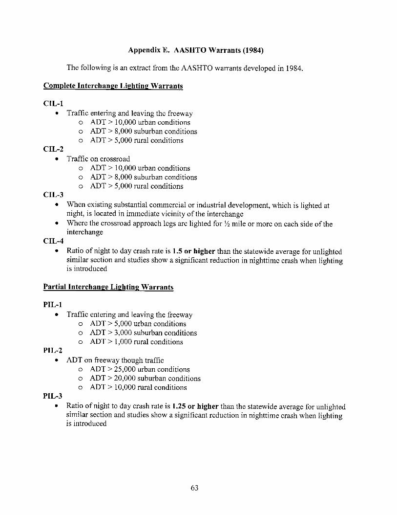
Appendix E. AASHTO Warrants (1984)

The following is an extract from the AASHTO warrants developed in 1984.

Complete Interchange Lighting Warrants

CIL-1

CIL-2

CIL-3

CIL-4

Traffic entering and leaving the freeway o ADT > 10,000 urban conditions o ADT > 8,000 suburban conditions o ADT > 5,000 rural conditions

Traffic on crossroad o ADT > 10,000 urban conditions o ADT > 8,000 suburban conditions o ADT > 5,000 rural conditions

When existing substantial commercial or industrial development, which is lighted at night, is located in immediate vicinity of the interchange Where the crossroad approach legs are lighted for ½ mile or more on each side of the interchange

Ratio of night to day crash rate is 1.5 or higher than the statewide average for unlighted similar section and studies show a significant reduction in nighttime crash when lighting is introduced

Partial Interchange Lighting Warrants

PIL-1

PIL-2

PIL-3

Traffic entering and leaving the freeway o ADT > 5,000 urban conditions o ADT > 3,000 suburban conditions o ADT > 1,000 rural conditions

ADT on freeway though traffic o ADT > 25,000 urban conditions o ADT > 20,000 suburban conditions o ADT > 10,000 rural conditions

Ratio of night to day crash rate is 1.25 or higher than the statewide average for unlighted similar section and studies show a significant reduction in nighttime crash when lighting is introduced

63

Appendix F. NCHRP Forms for the Four Examples of Application of the Screening Method

The following are the NCHRP forms as filled to address the need for visibility improvement formulated for the examples 1 to 4.

65

ANALYZING LIGHTING NEEDS

67

ANALYZING LIGHTING NEEDS

68

A©dd•.nt

ANALYZING LIGHTING: NEEDS

FORM

FOR h!ON.CO•TROL• A•$ FACIIa•Fy LIGHTING

< 1.0

G £OM •RIC TOTAL OP£MTIONAL TOTAL EN VIRONME,NTAL TOTAL ACCIDENT TOTAL

WA R.•TLNG COND•ION

12;. 2.0': 0 0 S+0

70

SCREENING METHODOLOGY FOR NEEDS OF ROADWAY · SCREENING METHODOLOGY FOR NEEDS OF ROADWAY LIGHTING...

Documents

Transcript of SCREENING METHODOLOGY FOR NEEDS OF ROADWAY · SCREENING METHODOLOGY FOR NEEDS OF ROADWAY LIGHTING...