Scientific Reasoning and Inference: A Bayesian...

Scientific Reasoning and Inference: A Bayesian Approach"que la théorie des probabilités n'est, au fond, que le bon sens réduit au calcul" S. P. Laplace (1814)"Therefore the true logic for this world is the calculus of probabilities" J. C. Maxwell (1850)“This theorem (due to Bayes) is to the theory of probability what Pythagoras's' theorem is to geometry” Harold Jeffreys (1961)

Scientists collect or measure data. But however much we collect, and however carefully we measure, we will always have incomplete information. How then do we make sound scientific inferences in the presence of uncertainty so as advance our knowledge and build sound theories of how the world works? That is the subject of this course

Texts and further reading suggestions

Sivia, D., and J. Skilling. 2006. Data Analysis, a Bayesian Tutorial. Oxford Science Publications. Oxford: Oxford University Press.

Iversen, Gudmund R. 1984. Bayesian Statistical Inference. Vol. 43. Quantitative Applications in the Social Sciences. Beverly Hills: Sage Publications.

Dewney, Allen. 2012. Think Bayes. 1.08. Green Tea Press.Jeffreys, Harold. 1973. Scientific Inference. 3d ed. Cambridge [Eng.]: Cambridge University Press.MacKay, David J. C. 2003. Information Theory, Inference, and Learning Algorithms. Cambridge, U.K.: Cambridge University Press.Sontag, Sherry. 1998. Blind Man’s Bluff : The Untold Story of American Submarine Espionage  . New York: Public Affairs.

1 Scientific Reasoning and Inference, K. A. Sharp, 2016

Our fundamental given: Data“Data compression and data modelling(analysis) are one and the same ” (MacKay 2003)

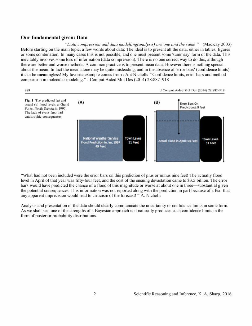
Before starting on the main topic, a few words about data: The ideal is to present all the data, either in tables, figures or some combination. In many cases this is not possible, and one must present some 'summary' form of the data. This inevitably involves some loss of information (data compression). There is no one correct way to do this, although there are better and worse methods. A common practice is to present mean data. However there is nothing special about the mean: In fact the mean alone may be quite misleading, and in the absence of 'error bars' (confidence limits) it can be meaningless! My favorite example comes from : Ant Nicholls “Confidence limits, error bars and method comparison in molecular modeling.” J Comput Aided Mol Des (2014) 28:887–918

“What had not been included were the error bars on this prediction of plus or minus nine feet! The actually flood level in April of that year was fifty-four feet, and the cost of the ensuing devastation came to $3.5 billion. The error bars would have predicted the chance of a flood of this magnitude or worse at about one in three—substantial given the potential consequences. This information was not reported along with the prediction in part because of a fear that any apparent imprecision would lead to criticism of the forecast! “ A. Nicholls

Analysis and presentation of the data should clearly communicate the uncertainty or confidence limits in some form. As we shall see, one of the strengths of a Bayesian approach is it naturally produces such confidence limits in the form of posterior probability distributions.


Best practice for plotting: The two most common cases

1) Category or population data

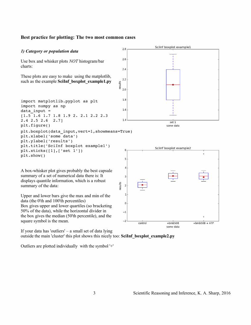
Use box and whisker plots NOT histogram/bar charts:

These plots are easy to make using the matplotlib, such as the example SciInf_boxplot_example1.py

import matplotlib.pyplot as plt import numpy as np data_input = [1.5 1.6 1.7 1.8 1.9 2. 2.1 2.2 2.3 2.4 2.5 2.6 2.7]plt.figure()

plt.boxplot(data_input,vert=1,showmeans=True) plt.xlabel('some data') plt.ylabel('results') plt.title('SciInf boxplot example1') plt.xticks([1],['set 1']) plt.show()

A box-whisker plot gives probably the best capsule summary of a set of numerical data there is: It displays quantile information, which is a robust summary of the data:

Upper and lower bars give the max and min of the data (the 0'th and 100'th percentiles) Box gives upper and lower quartiles (so bracketing 50% of the data), while the horizontal divider in the box gives the median (50'th percentile), and the square symbol is the mean.

If your data has 'outliers' – a small set of data lying outside the main 'cluster' this plot shows this nicely too: SciInf_boxplot_example2.py

Outliers are plotted individually with the symbol '+'


2) X-Y scatter plots with linear regression (trend line)

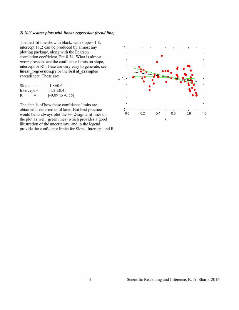
The best fit line show in black, with slope=-1.8, intercept 11.2 can be produced by almost any plotting package, along with the Pearson correlation coefficient, R=-0.34. What is almost never provided are the confidence limits on slope, intercept or R! These are very easy to generate, see linear_regression.py or the SciInf_examples spreadsheet. These are:

Slope = -1.8±0.6Intercept = 11.2 ±0.4R = [-0.09 to -0.55]

The details of how these confidence limits are obtained is deferred until later. But best practice would be to always plot the +/- 2-sigma fit lines on the plot as well (green lines) which provides a good illustration of the uncertainty, and in the legend provide the confidence limits for Slope, Intercept and R.


Now back to our main topic: Scientific Inference and Reasoning

What we won't be talking about much, if at all:


Our fundamental concept: ProbabilityThe traditional two-value logic of Aristotle, Boole etc.Premise: If A is true then B is true If it is raining then it must be cloudy

Observation: A is true It is rainingInference: B is true Therefore it is cloudy

Observation: B is false It is not cloudyInference: A is false Therefore it is not raining

We are dealing with events that are either certain or impossible. As scientists we are much more interested in the reverse inferences. For example

Observation: It is cloudy. Question: Is it raining? (If B is true, is A true?)

Observation: It is not raining. Question: Is it cloudy? (If A is false, is B true?)

Now we are dealing with uncertainty, or lack of complete knowledge.

Defining ProbabilityIf we represent certainty by a probability of 1 and impossibility by a probability of 0, what exactly do we mean by an intermediate probability (0 < prob < 1)? Take prob=½. In some interpretations, this means that some event happens half of the time, like heads or tails when flipping a fair coin. However, defining probability in this way is problematic: We would expect to get exactly 50% H's only if we flipped an infinite number of times, which is impossible. A finite sequence of coin flips will give a certain number of H and T- these are frequencies, NOT probabilities. We may well have an unequal number of H's and T's. Do we take the precise fraction as the probability? What about a new series of flips giving a slightly different fraction? The frequency in any experiment turns out only to be an estimate of some probability, not a definition. The 'frequentist' definition of probability is difficult to give without circular arguments.

The alternative definition is that probability is a measure of our uncertainty, or lack of knowledge about some event or situation. This is also known as the subjectivist interpretation, because it is possible for a different person to have different states of knowledge about a situation and so assign a different probability to an event than you. Alternatively, we may acquire new knowledge and so change the probability we assign to the same event. Note that subjective ≠ arbitrary. Two rational intelligent people should assign the same probability to an event given the same background and knowledge. If not, then it would be possible for one person to consistently win money from the other by offering the correct odds. This is the so called “Dutch Book Argument”!

Example 1. The unfair coin


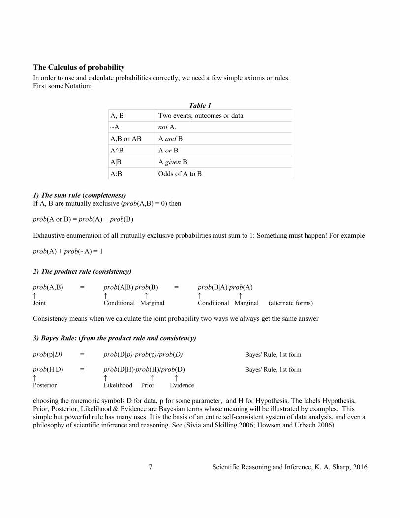
The Calculus of probabilityIn order to use and calculate probabilities correctly, we need a few simple axioms or rules.First some Notation:

Table 1A, B Two events, outcomes or data

~A not A.

A,B or AB A and B

A^B A or B

A|B A given B

A:B Odds of A to B

1) The sum rule (completeness)If A, B are mutually exclusive (prob(A,B) = 0) then

prob(A or B) = prob(A) + prob(B)

Exhaustive enumeration of all mutually exclusive probabilities must sum to 1: Something must happen! For example

prob(A) + prob(~A) = 1

2) The product rule (consistency)

prob(A,B) = prob(A|B)∙prob(B) = prob(B|A)∙prob(A)↑ ↑ ↑ ↑ ↑Joint Conditional Marginal Conditional Marginal (alternate forms)

Consistency means when we calculate the joint probability two ways we always get the same answer

3) Bayes Rule: (from the product rule and consistency)

prob(p|D) = prob(D|p)∙prob(p)/prob(D) Bayes' Rule, 1st form

prob(H|D) = prob(D|H)∙prob(H)/prob(D) Bayes' Rule, 1st form↑ ↑ ↑ ↑Posterior Likelihood Prior Evidence

choosing the mnemonic symbols D for data, p for some parameter, and H for Hypothesis. The labels Hypothesis, Prior, Posterior, Likelihood & Evidence are Bayesian terms whose meaning will be illustrated by examples. This simple but powerful rule has many uses. It is the basis of an entire self-consistent system of data analysis, and even a philosophy of scientific inference and reasoning. See (Sivia and Skilling 2006; Howson and Urbach 2006)


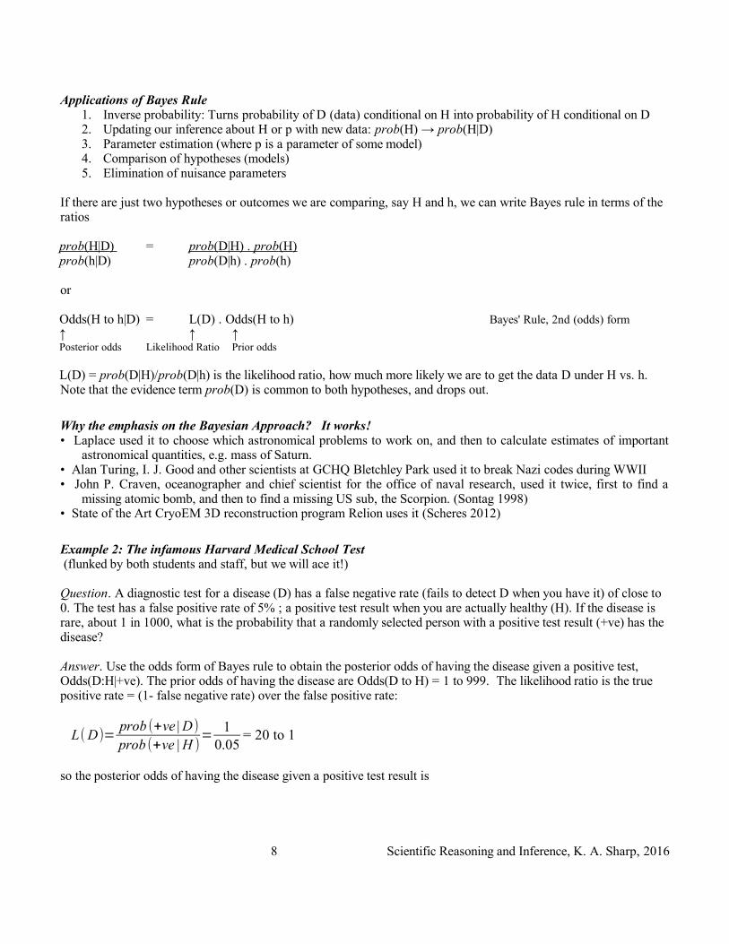
Applications of Bayes Rule1. Inverse probability: Turns probability of D (data) conditional on H into probability of H conditional on D2. Updating our inference about H or p with new data: prob(H) → prob(H|D)3. Parameter estimation (where p is a parameter of some model)4. Comparison of hypotheses (models)5. Elimination of nuisance parameters

If there are just two hypotheses or outcomes we are comparing, say H and h, we can write Bayes rule in terms of the ratios

prob (H|D ) = prob ( D|H) . prob (H ) prob(h|D) prob(D|h) . prob(h)

or

Odds(H to h|D) = L(D) . Odds(H to h) Bayes' Rule, 2nd (odds) form↑ ↑ ↑Posterior odds Likelihood Ratio Prior odds

L(D) = prob(D|H)/prob(D|h) is the likelihood ratio, how much more likely we are to get the data D under H vs. h. Note that the evidence term prob(D) is common to both hypotheses, and drops out.

Why the emphasis on the Bayesian Approach? It works!• Laplace used it to choose which astronomical problems to work on, and then to calculate estimates of important

astronomical quantities, e.g. mass of Saturn.• Alan Turing, I. J. Good and other scientists at GCHQ Bletchley Park used it to break Nazi codes during WWII• John P. Craven, oceanographer and chief scientist for the office of naval research, used it twice, first to find a

missing atomic bomb, and then to find a missing US sub, the Scorpion. (Sontag 1998)• State of the Art CryoEM 3D reconstruction program Relion uses it (Scheres 2012)

Example 2: The infamous Harvard Medical School Test (flunked by both students and staff, but we will ace it!)

Question. A diagnostic test for a disease (D) has a false negative rate (fails to detect D when you have it) of close to 0. The test has a false positive rate of 5% ; a positive test result when you are actually healthy (H). If the disease is rare, about 1 in 1000, what is the probability that a randomly selected person with a positive test result (+ve) has the disease?

Answer. Use the odds form of Bayes rule to obtain the posterior odds of having the disease given a positive test, Odds(D:H|+ve). The prior odds of having the disease are Odds(D to H) = 1 to 999. The likelihood ratio is the true positive rate = (1- false negative rate) over the false positive rate:

L(D)=prob (+ve | D)

prob (+ve | H )=

10.05

= 20 to 1

so the posterior odds of having the disease given a positive test result is


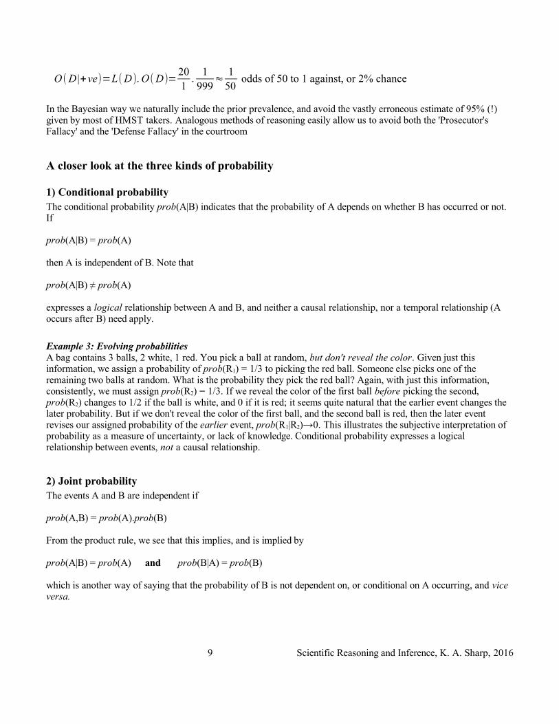
O(D |+ve)=L(D).O( D)=201

.1

999≈

150

odds of 50 to 1 against, or 2% chance

In the Bayesian way we naturally include the prior prevalence, and avoid the vastly erroneous estimate of 95% (!) given by most of HMST takers. Analogous methods of reasoning easily allow us to avoid both the 'Prosecutor's Fallacy' and the 'Defense Fallacy' in the courtroom

A closer look at the three kinds of probability

1) Conditional probabilityThe conditional probability prob(A|B) indicates that the probability of A depends on whether B has occurred or not. If

prob(A|B) = prob(A)

then A is independent of B. Note that

prob(A|B) ≠ prob(A)

expresses a logical relationship between A and B, and neither a causal relationship, nor a temporal relationship (A occurs after B) need apply.

Example 3: Evolving probabilitiesA bag contains 3 balls, 2 white, 1 red. You pick a ball at random, but don't reveal the color. Given just this information, we assign a probability of prob(R1) = 1/3 to picking the red ball. Someone else picks one of the remaining two balls at random. What is the probability they pick the red ball? Again, with just this information, consistently, we must assign prob(R2) = 1/3. If we reveal the color of the first ball before picking the second, prob(R2) changes to 1/2 if the ball is white, and 0 if it is red; it seems quite natural that the earlier event changes the later probability. But if we don't reveal the color of the first ball, and the second ball is red, then the later event revises our assigned probability of the earlier event, prob(R1|R2)→0. This illustrates the subjective interpretation of probability as a measure of uncertainty, or lack of knowledge. Conditional probability expresses a logical relationship between events, not a causal relationship.

2) Joint probabilityThe events A and B are independent if

prob(A,B) = prob(A).prob(B)

From the product rule, we see that this implies, and is implied by

prob(A|B) = prob(A) and prob(B|A) = prob(B)

which is another way of saying that the probability of B is not dependent on, or conditional on A occurring, and vice versa.


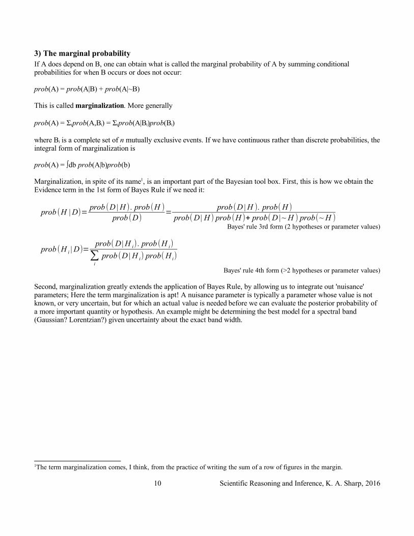
3) The marginal probabilityIf A does depend on B, one can obtain what is called the marginal probability of A by summing conditional probabilities for when B occurs or does not occur:

prob(A) = prob(A|B) + prob(A|~B)

This is called marginalization. More generally

prob(A) = Σιprob(A,Bi) = Σιprob(A|Bi)prob(Bi)

where Bi is a complete set of n mutually exclusive events. If we have continuous rather than discrete probabilities, the integral form of marginalization is

prob(A) = ∫db prob(A|b)prob(b)

Marginalization, in spite of its name1, is an important part of the Bayesian tool box. First, this is how we obtain the Evidence term in the 1st form of Bayes Rule if we need it:

prob (H | D)=prob (D | H ) . prob (H )

prob (D)=

prob (D | H ). prob(H )

prob(D | H ) prob (H )+ prob(D |~ H ) prob(~ H )

Bayes' rule 3rd form (2 hypotheses or parameter values)

prob (H i | D)=prob(D | H i) . prob (H i)

∑i

prob (D | H i) prob(H i)

Bayes' rule 4th form (>2 hypotheses or parameter values)

Second, marginalization greatly extends the application of Bayes Rule, by allowing us to integrate out 'nuisance' parameters; Here the term marginalization is apt! A nuisance parameter is typically a parameter whose value is not known, or very uncertain, but for which an actual value is needed before we can evaluate the posterior probability of a more important quantity or hypothesis. An example might be determining the best model for a spectral band (Gaussian? Lorentzian?) given uncertainty about the exact band width.

1The term marginalization comes, I think, from the practice of writing the sum of a row of figures in the margin.


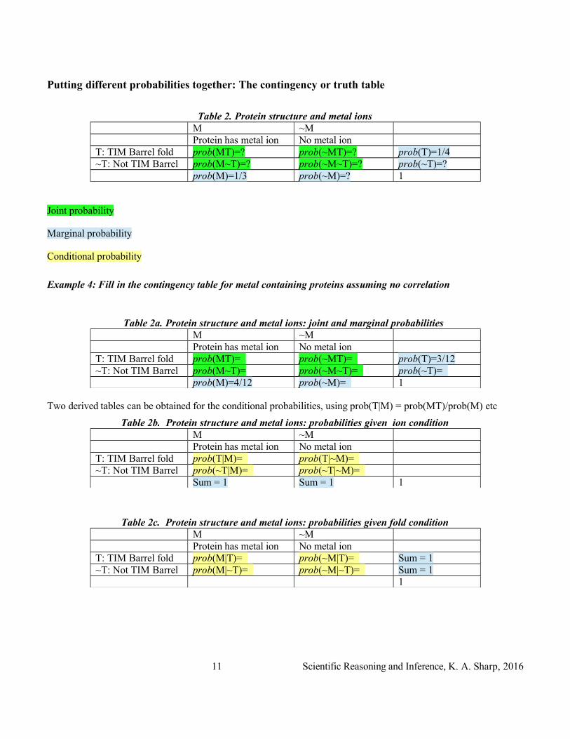
Putting different probabilities together: The contingency or truth table

Table 2. Protein structure and metal ionsM ~MProtein has metal ion No metal ion

T: TIM Barrel fold prob(MT)=? prob(~MT)=? prob(T)=1/4~T: Not TIM Barrel prob(M~T)=? prob(~M~T)=? prob(~T)=?

prob(M)=1/3 prob(~M)=? 1

Joint probability

Marginal probability

Conditional probability

Example 4: Fill in the contingency table for metal containing proteins assuming no correlation

Table 2a. Protein structure and metal ions: joint and marginal probabilities M ~MProtein has metal ion No metal ion

T: TIM Barrel fold prob(MT)= prob(~MT)= prob(T)=3/12~T: Not TIM Barrel prob(M~T)= prob(~M~T)= prob(~T)=

prob(M)=4/12 prob(~M)= 1

Two derived tables can be obtained for the conditional probabilities, using prob(T|M) = prob(MT)/prob(M) etc

Table 2b. Protein structure and metal ions: probabilities given ion conditionM ~MProtein has metal ion No metal ion

T: TIM Barrel fold prob(T|M)= prob(T|~M)= ~T: Not TIM Barrel prob(~T|M)= prob(~T|~M)=

Sum = 1 Sum = 1 1

Table 2c. Protein structure and metal ions: probabilities given fold conditionM ~MProtein has metal ion No metal ion

T: TIM Barrel fold prob(M|T)= prob(~M|T)= Sum = 1~T: Not TIM Barrel prob(M|~T)= prob(~M|~T)= Sum = 1

1


Bayes' Rule in Action!

Outline of steps in Bayesian analysis1. Determine prior probability for parameters: Example parameters include population identity, the mean, the

variance, the correlation coefficient, slope, intercept etc.2. Compute probability (Likelihood) function that data could be produced as a function of parameters. Use

Analytical approximations or Numerical methods as appropriate.3. Use Bayes rule to invert probability, getting posterior distribution for parameters. 4. Interpret and Summarize posterior distribution, get confidence intervals.

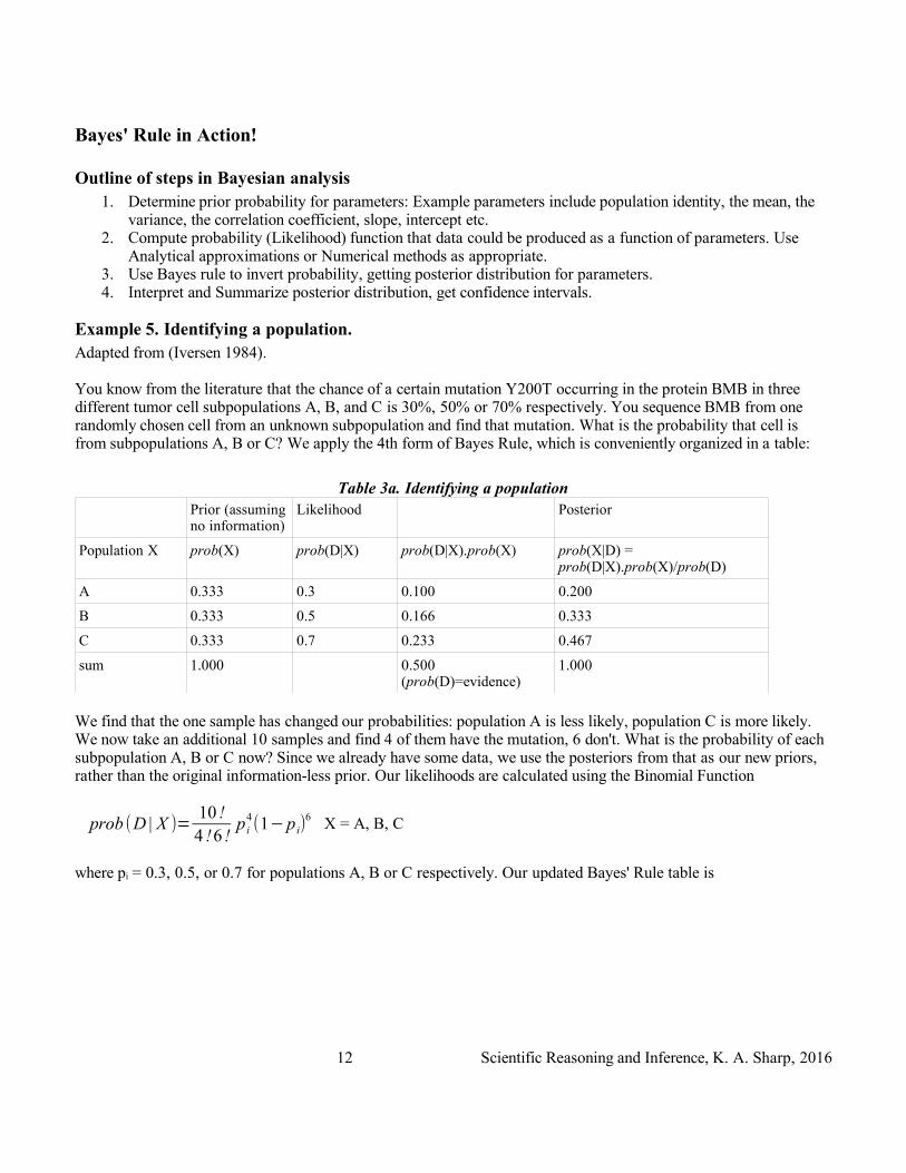
Example 5. Identifying a population. Adapted from (Iversen 1984).

You know from the literature that the chance of a certain mutation Y200T occurring in the protein BMB in three different tumor cell subpopulations A, B, and C is 30%, 50% or 70% respectively. You sequence BMB from one randomly chosen cell from an unknown subpopulation and find that mutation. What is the probability that cell is from subpopulations A, B or C? We apply the 4th form of Bayes Rule, which is conveniently organized in a table:

Table 3a. Identifying a populationPrior (assuming no information)

Likelihood Posterior

Population X prob(X) prob(D|X) prob(D|X).prob(X) prob(X|D) = prob(D|X).prob(X)/prob(D)

A 0.333 0.3 0.100 0.200

B 0.333 0.5 0.166 0.333

C 0.333 0.7 0.233 0.467

sum 1.000 0.500 (prob(D)=evidence)

1.000

We find that the one sample has changed our probabilities: population A is less likely, population C is more likely. We now take an additional 10 samples and find 4 of them have the mutation, 6 don't. What is the probability of each subpopulation A, B or C now? Since we already have some data, we use the posteriors from that as our new priors, rather than the original information-less prior. Our likelihoods are calculated using the Binomial Function

prob (D | X )=10 !4 !6 !

p i4(1−p i)

6 X = A, B, C

where pi = 0.3, 0.5, or 0.7 for populations A, B or C respectively. Our updated Bayes' Rule table is


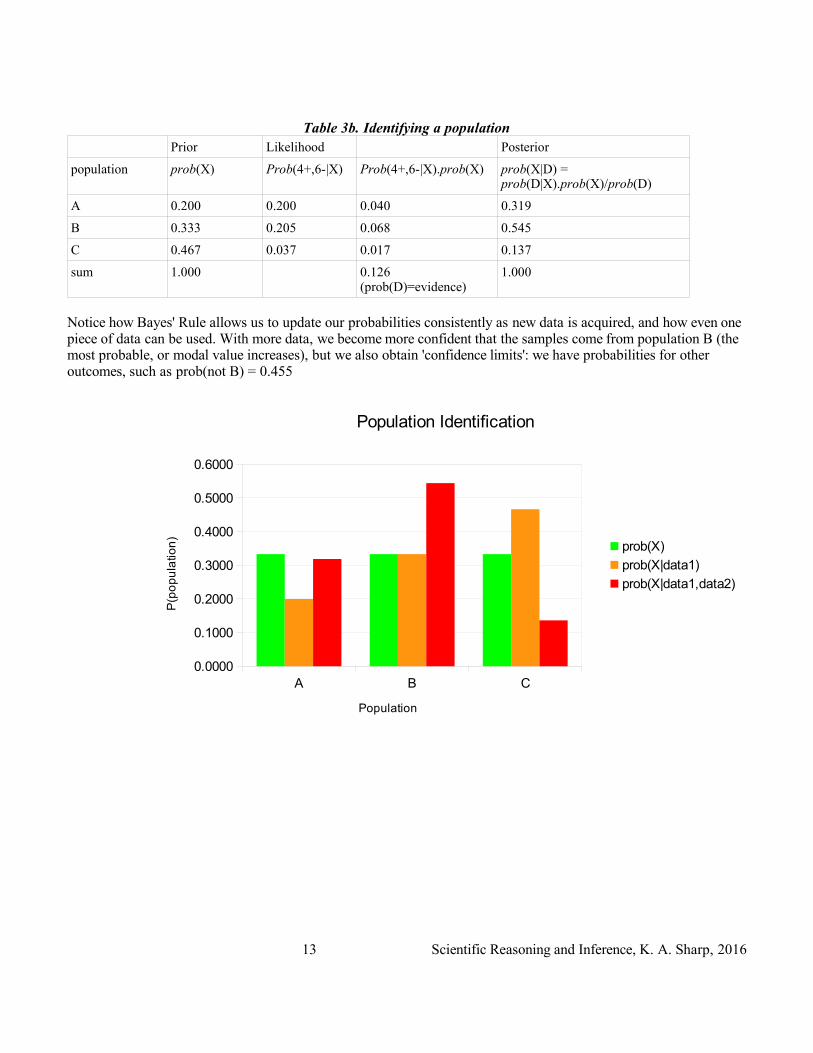
Table 3b. Identifying a populationPrior Likelihood Posterior

population prob(X) Prob(4+,6-|X) Prob(4+,6-|X).prob(X) prob(X|D) = prob(D|X).prob(X)/prob(D)

A 0.200 0.200 0.040 0.319

B 0.333 0.205 0.068 0.545

C 0.467 0.037 0.017 0.137

sum 1.000 0.126 (prob(D)=evidence)

1.000

Notice how Bayes' Rule allows us to update our probabilities consistently as new data is acquired, and how even one piece of data can be used. With more data, we become more confident that the samples come from population B (the most probable, or modal value increases), but we also obtain 'confidence limits': we have probabilities for other outcomes, such as prob(not B) = 0.455


A B C0.0000

0.1000

0.2000

0.3000

0.4000

0.5000

0.6000

Population Identification

prob(X)

prob(X|data1)

prob(X|data1,data2)

Population

P(p

op

ula

tion

)

Example 6. Parameter Estimation: A proportion, fraction or probability type parameter.Adapted from (Sivia and Skilling 2006). Python program: ProportionParameter.py

In example 5 “Identifying a population” our hypothesis space was threefold: this cell came from population A, from population B, or from population C. Alternatively, we may say that the parameter describing the chance of mutation in the BMB protein in the sample cell could take on just 3 fixed, discrete values: 30%, 50% or 70%. More generally, a parameter describing a fraction, percentage, proportion or probability can vary continuously between 0 and 100%. Define the parameter f as the probability of a mutation E100M in protein GCB. The data in our experiment is the number M of mutations found in N samples

Outline of steps in Bayesian analysis1. Determine prior probability for f={0-1}2. Compute probability (Likelihood) that data (M samples with mutations, N-M without mutations) could be

produced by given a certain probability of f in a single sample.3. Use Bayes rule to invert probability, getting posterior (updated) probability of f given data.

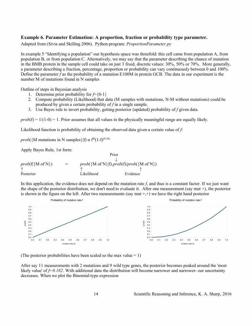
prob(f) = 1/(1-0) = 1. Prior assumes that all values in the physically meaningful range are equally likely.

Likelihood function is probability of obtaining the observed data given a certain value of f:

prob({M mutations in N samples}|f) α fM(1-f)(N-M)

Apply Bayes Rule, 1st form:Prior ↓

prob(f|{M of N}) = prob({M of N}|f).prob(f)/prob({M of N})↑ ↑ ↑Posterior Likelihood Evidence

In this application, the evidence does not depend on the mutation rate f, and thus is a constant factor. If we just want the shape of the posterior distribution, we don't need to evaluate it. After one measurement (say mut +), the posterior is shown in the figure on the left. After two measurements (say mut +,+) we have the right hand posterior

(The posterior probabilities have been scaled so the max value = 1)

After say 11 measurements with 2 mutations and 9 wild type genes, the posterior becomes peaked around the 'most likely value' of f=0.182. With additional data the distribution will become narrower and narrower- our uncertainty decreases. When we plot the Binomial-type expression


0.0 0.1 0.2 0.3 0.4 0.5 0.6 0.7 0.8 0.9 1.00.0

0.1

0.2

0.3

0.4

0.5

0.6

0.7

0.8

0.9

1.0

Probability of mutation rate f

mutation rate (f)

pro

b(f

)

0.0 0.1 0.2 0.3 0.4 0.5 0.6 0.7 0.8 0.9 1.00.0

0.1

0.2

0.3

0.4

0.5

0.6

0.7

0.8

0.9

1.0


mutation rate (f)

pro

b(f

)

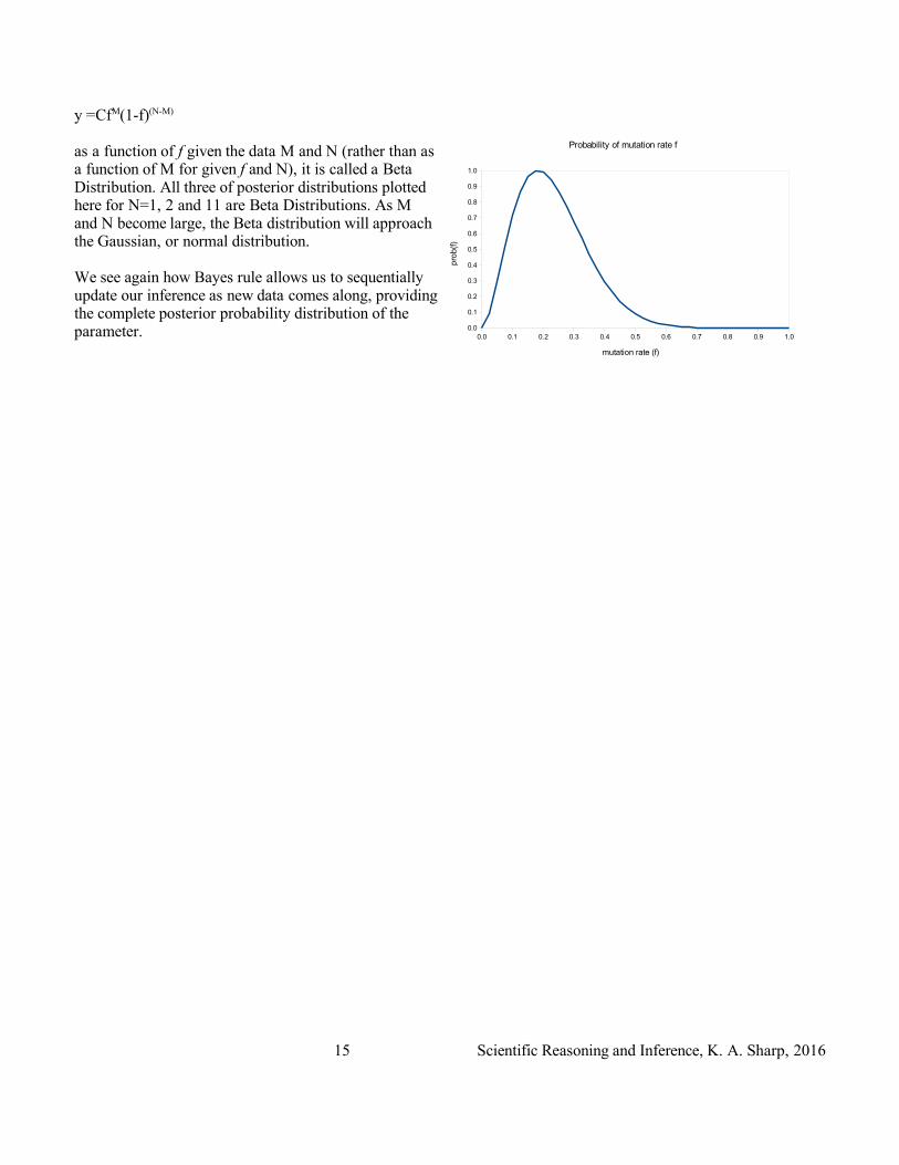
y =CfM(1-f)(N-M)

as a function of f given the data M and N (rather than as a function of M for given f and N), it is called a Beta Distribution. All three of posterior distributions plotted here for N=1, 2 and 11 are Beta Distributions. As M and N become large, the Beta distribution will approach the Gaussian, or normal distribution.

We see again how Bayes rule allows us to sequentially update our inference as new data comes along, providing the complete posterior probability distribution of the parameter.


0.0 0.1 0.2 0.3 0.4 0.5 0.6 0.7 0.8 0.9 1.00.0

0.1

0.2

0.3

0.4

0.5

0.6

0.7

0.8

0.9

1.0


mutation rate (f)

pro

b(f)

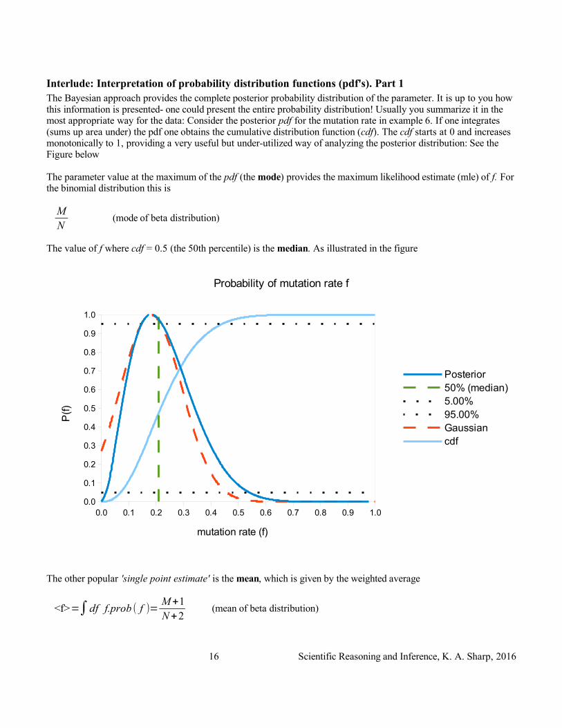
Interlude: Interpretation of probability distribution functions (pdf's). Part 1The Bayesian approach provides the complete posterior probability distribution of the parameter. It is up to you how this information is presented- one could present the entire probability distribution! Usually you summarize it in the most appropriate way for the data: Consider the posterior pdf for the mutation rate in example 6. If one integrates (sums up area under) the pdf one obtains the cumulative distribution function (cdf). The cdf starts at 0 and increases monotonically to 1, providing a very useful but under-utilized way of analyzing the posterior distribution: See the Figure below

The parameter value at the maximum of the pdf (the mode) provides the maximum likelihood estimate (mle) of f. For the binomial distribution this is

MN

(mode of beta distribution)

The value of f where cdf = 0.5 (the 50th percentile) is the median. As illustrated in the figure

The other popular 'single point estimate' is the mean, which is given by the weighted average

<f>=∫df f.prob ( f )=M+1N+2

(mean of beta distribution)


0.0 0.1 0.2 0.3 0.4 0.5 0.6 0.7 0.8 0.9 1.00.0

0.1

0.2

0.3

0.4

0.5

0.6

0.7

0.8

0.9

1.0


Posterior50% (median)5.00%95.00%Gaussiancdf

mutation rate (f)

P(f

)

Although the mean gets the lion's share of attention in the literature and classes, there is no one best 'single point' summary for all situations. Remember, all data analysis is a form of data compression, so that there is an inevitable loss of information. The mean may be quite misleading for very asymmetric (skewed) or multi-peaked distributions. Besides, no single point estimate is useful without the confidence limits or uncertainties.

Again the cdf comes in very handy. Picking off the parameter values corresponding to cdf =5 % and 95%, the interval f={0.075,0.45} contains 90% of the probability. Put another way, given the data accumulated so far, there is a 10% chance that f is either less than 0.075 or greater than 0.45. The quantile limits such as 5%/95% or 2.5%/97.5% are highly recommended : they are robust, apply to asymmetric distributions and are self explanatory.

More popular, although less robust are standard deviations (variances). For the beta distribution, the 2-sigma confidence intervals are:

f max±2√ f max (1− f max)

(N +3)

Note this range is symmetric, even if the distribution is not!. Another measure of spread is the width at half height of maximum, which is common in the world of spectroscopy.

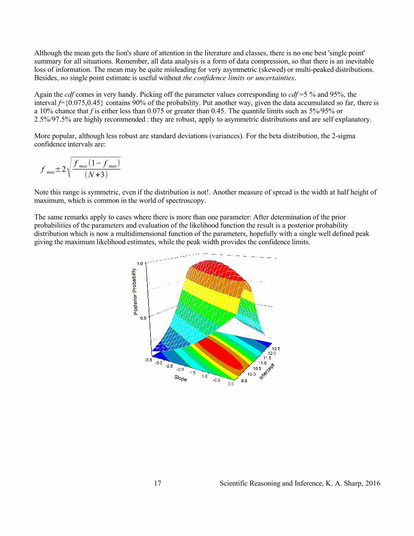
The same remarks apply to cases where there is more than one parameter: After determination of the prior probabilities of the parameters and evaluation of the likelihood function the result is a posterior probability distribution which is now a multidimensional function of the parameters, hopefully with a single well defined peak giving the maximum likelihood estimates, while the peak width provides the confidence limits.


Example 7a. Estimation of population size part 1: Tag and ReleaseAfter (Webster, A. J. and Kemp, R. 2013) Python program: TagAndRelease.py

You need to determine the number of repressor molecules in a cell. For experimental reasons you cannot simply extract and quantify the total amount (Maybe you are studying live cells over time). You radio-label a purified or expressed sample of the repressor, introduce a known number of tagged molecules, Nt, wait a suitable time, extract a small aliquot of the cell interior in which you find Nc repressor molecules, of which Nm are labelled. What is the estimate of the total population of molecules N? This is the 'Tag and Release' method of population size estimation used for example by wild life biologists to estimate fish populations in lakes.

Your sample has a fraction f=Nm/Nc which are labelled. A plausible estimate of N is to assume that this fraction is representative of the entire population, so

N=N t

f=

N t N c

N m

Lincoln-Petersen mle estimate

However, to obtain the all-important confidence limits, we need to apply Bayes theorem. Given the number of tagged molecules, Nt and the number of molecules in your assay sample Nc, the posterior distribution for N is proportional to the likelihood function (obtained from the hypergeometric distribution. See appendix)

prob (N | N t , N c , N m)α prob (N m | N , N t , N c)α(N−N c)!(N −N t)!

N !(N−(N t+N c−N m))!

The prior assumes all values of N ≥Nt are equally likely.

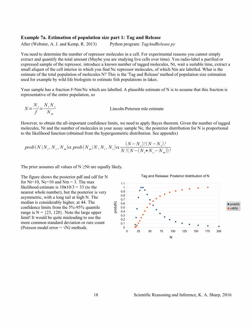
The figure shows the posterior pdf and cdf for N for Nt=10, Nc=10 and Nm = 3. The max likelihood estimate is 10x10/3 = 33 (to the nearest whole number), but the posterior is very asymmetric, with a long tail at high N. The median is considerably higher, at 44. The confidence limits from the 5%-95% quantile range is N = {23, 120}. Note the large upper limit! It would be quite misleading to use the more common standard deviation or rare count (Poisson model error = √N) methods.


0 25 50 75 100 125 150 175 2000

0.10.20.30.40.50.60.70.80.9

11.1

Tag and Release: Posterior distribution of N

prob(N)

cdf(N)

N

pro

b(N

)

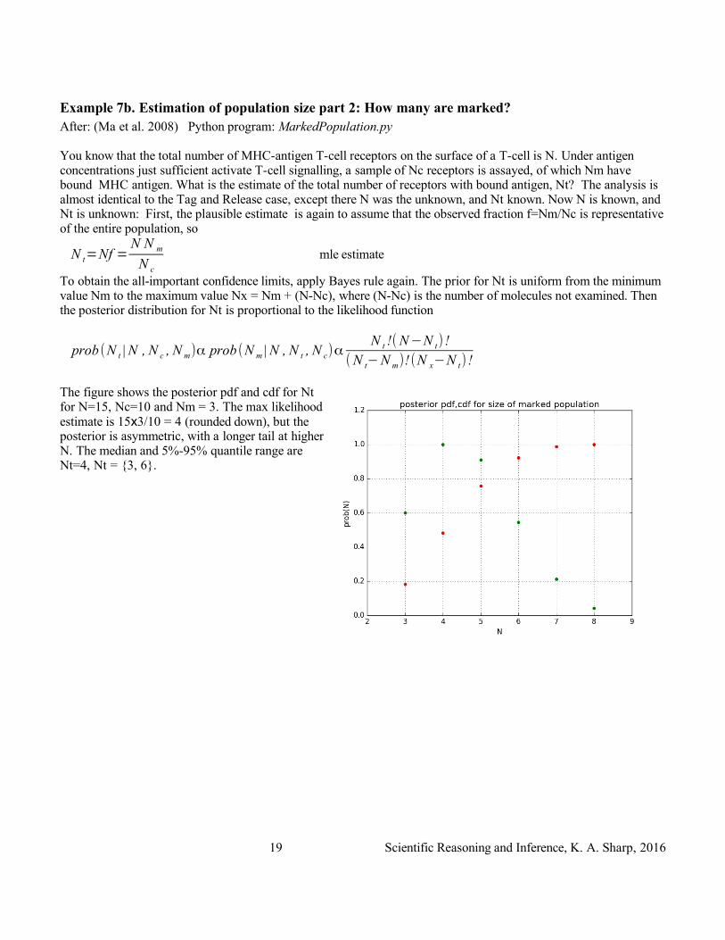
Example 7b. Estimation of population size part 2: How many are marked?After: (Ma et al. 2008) Python program: MarkedPopulation.py

You know that the total number of MHC-antigen T-cell receptors on the surface of a T-cell is N. Under antigen concentrations just sufficient activate T-cell signalling, a sample of Nc receptors is assayed, of which Nm have bound MHC antigen. What is the estimate of the total number of receptors with bound antigen, Nt? The analysis is almost identical to the Tag and Release case, except there N was the unknown, and Nt known. Now N is known, and Nt is unknown: First, the plausible estimate is again to assume that the observed fraction f=Nm/Nc is representative of the entire population, so

N t=Nf =N N m

N c

mle estimate

To obtain the all-important confidence limits, apply Bayes rule again. The prior for Nt is uniform from the minimum value Nm to the maximum value Nx = Nm + (N-Nc), where (N-Nc) is the number of molecules not examined. Then the posterior distribution for Nt is proportional to the likelihood function

prob (N t | N , N c , N m)α prob (N m | N , N t , N c)αN t !(N−N t) !

(N t−N m)!(N x−N t) !

The figure shows the posterior pdf and cdf for Nt for N=15, Nc=10 and Nm = 3. The max likelihood estimate is 15x3/10 = 4 (rounded down), but the posterior is asymmetric, with a longer tail at higher N. The median and 5%-95% quantile range are Nt=4, Nt = {3, 6}.


Example 8. Estimation of population size part 3: How big is a familyAdapted from: (Dewney 2012) Python program: FamilySize.py

You ask a randomly selected person what birth order child they are. They answer “the M'th child.” How many children are there in that family? The most likely answer is N=M (!) Put another way you are most likely talking to the youngest child. Let's take M=2 for example.

Clearly N=1 is impossible: In terms of probability, the likelihood prob(M=2|N=1) = 0, so therefore the posterior prob(N=1|M=2) = 0. Collecting the results for N≥M:

Table 4. The likelihoods for different family size NPopulation Size Likelihood prob(M=2|N)

N = 1 0

N = 2 1/2

N = 3 1/3

N > 3 1/N

so the probability decreases as N increases. Assuming that each value of N is equally likely (Uniform prior) the posterior will have the form:

prob(N|M) = 0 for N≤Mprob(N|M) = 1/N for N≥M

This another type of long tailed posterior

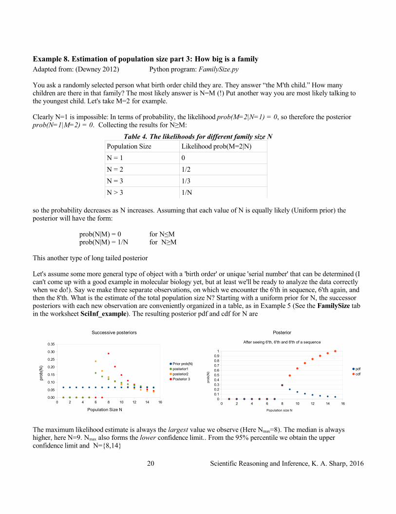
Let's assume some more general type of object with a 'birth order' or unique 'serial number' that can be determined (I can't come up with a good example in molecular biology yet, but at least we'll be ready to analyze the data correctly when we do!). Say we make three separate observations, on which we encounter the 6'th in sequence, 6'th again, and then the 8'th. What is the estimate of the total population size N? Starting with a uniform prior for N, the successor posteriors with each new observation are conveniently organized in a table, as in Example 5 (See the FamilySize tab in the worksheet SciInf_example). The resulting posterior pdf and cdf for N are

The maximum likelihood estimate is always the largest value we observe (Here Nmax=8). The median is always higher, here N=9. Nmax also forms the lower confidence limit.. From the 95% percentile we obtain the upper confidence limit and N={8,14}


0 2 4 6 8 10 12 14 160.00

0.05

0.10

0.15

0.20

0.25

0.30

0.35

Successive posteriors

Prior prob(N)

posterior1

posterior2Posterior 3

Population Size N

pro

b(N

)

0 2 4 6 8 10 12 14 160

0.10.20.30.40.50.60.70.80.9

1

Posterior

After seeing 6'th, 6'th and 8'th of a sequence

pdf

cdf

Population size N

pro

b(N

)

Interlude: Where do we get prior distributions from?In all the examples so far, we assumed a uniform prior distribution: uniform between the different populations, for a fraction f between 0 and 1, for the number in a population. This seems intuitively reasonable, as without any specific information any value is as likely as another. However there is a more powerful principle for selecting priors in the absence on information:

The Maximum Entropy (MaxEnt) principle. Our prior probability distribution quantifies how much we already know before we have any data. We want to include as much prior information as we have in our models and inferences, but without assuming more than we actually know. In Bayesian lingo, we want the least informative prior. This leads naturally to the Maximum Information Entropy (MaxEnt) method. The Shannon/Jaynes information entropy is defined as

S {prob( i)}=−∑i=1

N

prob (i)ln prob( i)

for a discrete set of probabilities pk, and

S ( prob(q))=−∫d q prob(q) ln prob (q )

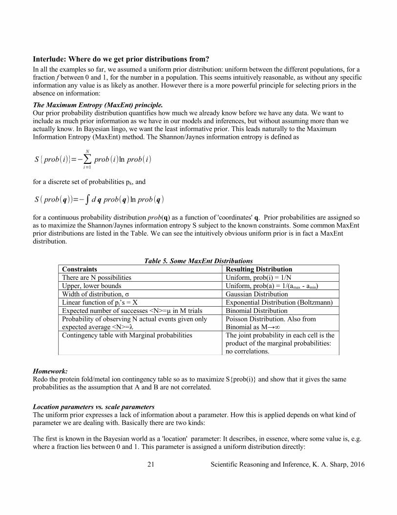
for a continuous probability distribution prob(q) as a function of 'coordinates' q. Prior probabilities are assigned so as to maximize the Shannon/Jaynes information entropy S subject to the known constraints. Some common MaxEnt prior distributions are listed in the Table. We can see the intuitively obvious uniform prior is in fact a MaxEnt distribution.

Table 5. Some MaxEnt DistributionsConstraints Resulting DistributionThere are N possibilities Uniform, prob(i) = 1/NUpper, lower bounds Uniform, prob(a) = 1/(amax - amin)Width of distribution, σ Gaussian DistributionLinear function of pi’s = X Exponential Distribution (Boltzmann)Expected number of successes <N>=μ in M trials Binomial DistributionProbability of observing N actual events given only expected average <N>=λ

Poisson Distribution. Also from Binomial as M→∞

Contingency table with Marginal probabilities The joint probability in each cell is the product of the marginal probabilities: no correlations.

Homework:Redo the protein fold/metal ion contingency table so as to maximize S{prob(i)} and show that it gives the same probabilities as the assumption that A and B are not correlated.

Location parameters vs. scale parametersThe uniform prior expresses a lack of information about a parameter. How this is applied depends on what kind of parameter we are dealing with. Basically there are two kinds:

The first is known in the Bayesian world as a 'location' parameter: It describes, in essence, where some value is, e.g. where a fraction lies between 0 and 1. This parameter is assigned a uniform distribution directly:


prob(x) = constant.

The second type describe the magnitude or scale of something. One clue we are dealing with a scale parameter is if, physically, must have a value greater than zero, for example a kinetic rate constant k. In this case the logarithm of the parameter is assigned a uniform distribution:

prob(ln k) = constant.

What this says is that there is equal prior probability that k lies between 0.1-1, between 1-10, between 10-100 etc. An equivalent and mathematically more convenient way to represent this is

prob (k )=constant

k

as we shall see in the next example.


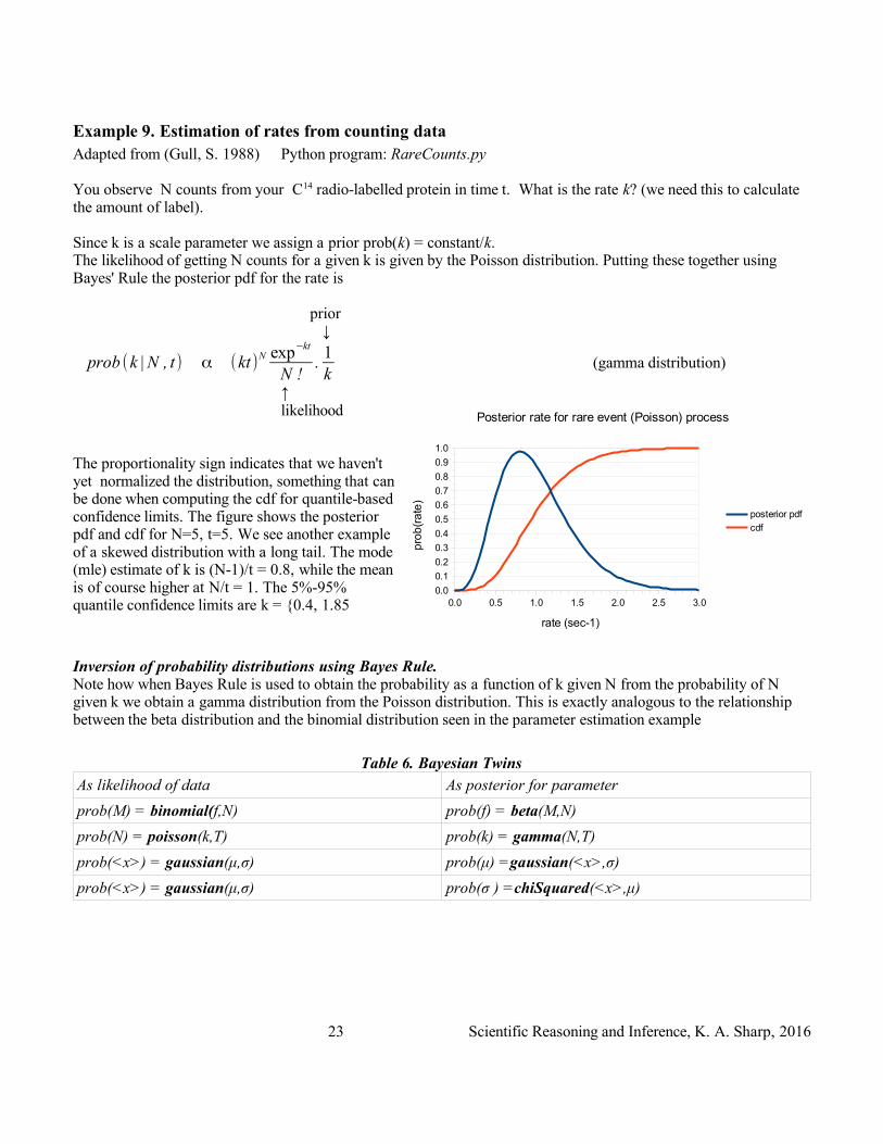
Example 9. Estimation of rates from counting dataAdapted from (Gull, S. 1988) Python program: RareCounts.py

You observe N counts from your C14 radio-labelled protein in time t. What is the rate k? (we need this to calculate the amount of label).

Since k is a scale parameter we assign a prior prob(k) = constant/k. The likelihood of getting N counts for a given k is given by the Poisson distribution. Putting these together using Bayes' Rule the posterior pdf for the rate is

prior ↓

prob (k | N , t) α (kt)N exp−kt

N !.1k

(gamma distribution)

↑likelihood

The proportionality sign indicates that we haven't yet normalized the distribution, something that can be done when computing the cdf for quantile-based confidence limits. The figure shows the posterior pdf and cdf for N=5, t=5. We see another example of a skewed distribution with a long tail. The mode (mle) estimate of k is (N-1)/t = 0.8, while the mean is of course higher at N/t = 1. The 5%-95% quantile confidence limits are k = {0.4, 1.85

Inversion of probability distributions using Bayes Rule. Note how when Bayes Rule is used to obtain the probability as a function of k given N from the probability of N given k we obtain a gamma distribution from the Poisson distribution. This is exactly analogous to the relationship between the beta distribution and the binomial distribution seen in the parameter estimation example

Table 6. Bayesian TwinsAs likelihood of data As posterior for parameter

prob(M) = binomial(f,N) prob(f) = beta(M,N)

prob(N) = poisson(k,T) prob(k) = gamma(N,T)

prob(<x>) = gaussian(μ,σ) prob(μ) =gaussian(<x>,σ)

prob(<x>) = gaussian(μ,σ) prob(σ ) =chiSquared(<x>,μ)


0.0 0.5 1.0 1.5 2.0 2.5 3.00.0

0.1

0.2

0.3

0.4

0.5

0.6

0.7

0.8

0.9

1.0

Posterior rate for rare event (Poisson) process

posterior pdf

cdf

rate (sec-1)

pro

b(r

ate

)

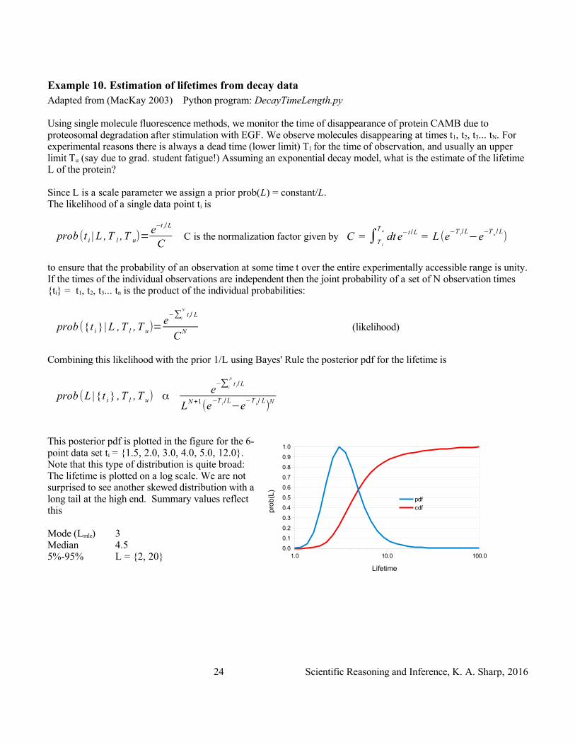
Example 10. Estimation of lifetimes from decay dataAdapted from (MacKay 2003) Python program: DecayTimeLength.py

Using single molecule fluorescence methods, we monitor the time of disappearance of protein CAMB due to proteosomal degradation after stimulation with EGF. We observe molecules disappearing at times t1, t2, t3... tN. For experimental reasons there is always a dead time (lower limit) Tl for the time of observation, and usually an upper limit Tu (say due to grad. student fatigue!) Assuming an exponential decay model, what is the estimate of the lifetime L of the protein?

Since L is a scale parameter we assign a prior prob(L) = constant/L. The likelihood of a single data point ti is

prob (t i | L ,T l ,T u)=e−t i/L

C C is the normalization factor given by C = ∫T l

T u

dt e−t /L = L (e−T l/L−e

−T u /L)

to ensure that the probability of an observation at some time t over the entire experimentally accessible range is unity. If the times of the individual observations are independent then the joint probability of a set of N observation times {ti} = t1, t2, t3... tn is the product of the individual probabilities:

prob ({t i }| L ,T l , T u)=e−∑i

N

ti/ L

CN (likelihood)

Combining this likelihood with the prior 1/L using Bayes' Rule the posterior pdf for the lifetime is

prob (L | { t i } ,T l , T u) α e−∑i

N

t i/L

LN +1(e

−T l /L−e

−T u/ L)

N

This posterior pdf is plotted in the figure for the 6-point data set ti = {1.5, 2.0, 3.0, 4.0, 5.0, 12.0}. Note that this type of distribution is quite broad: The lifetime is plotted on a log scale. We are not surprised to see another skewed distribution with a long tail at the high end. Summary values reflect this

Mode (Lmle) 3Median 4.55%-95% L = {2, 20}


1.0 10.0 100.00.0

0.1

0.2

0.3

0.4

0.5

0.6

0.7

0.8

0.9

1.0

pdf

cdf

Lifetime

pro

b(L

)

Example 11. Correlation Coefficients and Linear Regression See (Sivia and Skilling 2006; Mendenhall and Scheaffer 1973). Python program: LinearRegression.py

Experiments in which a set of N data {yi} are obtained as a function of some independent variable {xi} are common. These are often modelled by a linear dependence of yi on xi either by linear regression or calculation of the Pearson correlation coefficient R. It is very rare that confidence limits on the fitted parameters are given, although these are very easy to obtain. Let <> indicate an average over the N values.

Confidence limits for the correlation coefficient RThe Pearson correlation coefficient is given by

R=<xy> - <x>.<y>

√(<x2 >-<x>2)(<y2 >-<y>2

)

With a uniform prior for R = {-1...1}:

prob(R) = ½,

The approximate 95% confidence interval for the posterior distribution of R is the somewhat messy:

R '≈ tanh [arctanh( R)±2

√(n−3)]

(Mendenhall and Scheaffer 1973)

These intervals are plotted here for R = {0.2-0.9} and n = 10 points. The plot for negative correlations would simply be the mirror of this about the x-axis. Note the rather broad range of confidence intervals. At low absolute values of sample R, the lower bound includes r values of the opposite sign!

Linear Regression: Slope and InterceptTo fit a straight line, y = mx + c to a set of N points {xi}, {yi}, calculate

m=< xy >−< x >.< y >< x2 >−< x >2 , c=

< y> < x2 >−< x >.< xy >< x2 >−< x >2

The Pearson correlation coefficient R is given as above. But R is of limited importance in linear regression, in spite of the fact that it is often the only fit parameter reported. More important are the residuals (the difference between the actual y values and those calculated from the best fit line) and the confidence intervals of the fit parameters. The mean of the squares of the residuals (the variance of the residuals) is given by

χ2=

1N−2

∑ ( y i−(mxi+c ))2

From χ2 the variances in the best fit slope and intercept can be calculated


0 0.1 0.2 0.3 0.4 0.5 0.6 0.7 0.8 0.9 1

-0.6

-0.4

-0.2

0.0

0.2

0.4

0.6

0.8

1.0

R observed

R p

ost

eri

or

σmm2

=χ

2

N (< x2 >−< x >2), σ cc

2=

< x2 > .χ2

N (< x2 >−< x>2)

from which we can obtain the 95% confidence intervals as m±2σmm, and c±2σmc. These are not independent, however, as is clear from a cursory examination of an x-y plot with fitted line. The covariance between slope m and intercept c is

σmc2=

< x >χ2

N (< x2 >−< x >2)

The correlation coefficient between fit parameters (NOT between X and Y!) is

rmc=σmc2 /√σmm

2. σcc2

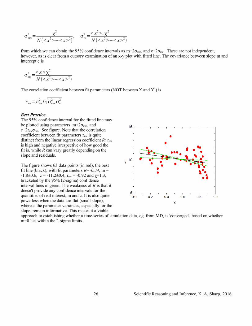
Best PracticeThe 95% confidence interval for the fitted line may be plotted using parameters m±2σmm, and c±2rmcσmc. See figure. Note that the correlation coefficient between fit parameters rmc is quite distinct from the linear regression coefficient R: rmc

is high and negative irrespective of how good the fit is, while R can vary greatly depending on the slope and residuals.

The figure shows 63 data points (in red), the best fit line (black), with fit parameters R=-0.34, m = -1.8±0.6, c = -11.2±0.4, rmc = -0.92 and χ=1.3, bracketed by the 95% (2-sigma) confidence interval lines in green. The weakness of R is that it doesn't provide any confidence intervals for the quantities of real interest, m and c. It is also quite powerless when the data are flat (small slope), whereas the parameter variances, especially for the slope, remain informative. This makes it a viable approach to establishing whether a time-series of simulation data, eg. from MD, is 'converged', based on whether m=0 lies within the 2-sigma limits.


Example 12. Estimation of the mean of data D = {x1...xn} with no prior data or informationSee (Gull, S. 1988)

Given a set of data {xi}, we believe that it comes from a population with unknown mean, μ which we wish to estimate. Each value xi differs from this mean due to some random factor (noise, measurement error, random perturbations etc). We only know that this random contribution has some magnitude. Then from the MaxEnt assumption the probability of each datum is

prob (x i |μ ,ϵ)=1

√2πϵ2

exp(−(x i−μ)2/2ϵ

2)

i.e the perturbation in the data point xi is normally distributed around 0, with standard deviation ε. The probability (likelihood) of the entire set of N points {xi} is the product of the probability for each point:

prob ({ x i}|μ ,ϵ) = Πi

N 1

√2πϵ2

exp(−(x i−μ)2/2ϵ

2) ∝ ϵ−N exp(−∑ (x i−μ)

2/2ϵ

2)

replacing the product of exponentials with the sum of exponent terms. In the second step we have omitted the constant factor as this does not affect the shape of the pdf. Using Bayes' rule the posterior distribution of the mean and the 'noise magnitude' is:

prob(μ ,σ |{ xi})= prob({ xi }|μ ,σ) prob(μ) prob (σ)/ prob({ xi })

To obtain the shape of the posterior pdf we don't need the 'evidence' term in the denominator since it does not depend on μ or ε. The priors for the 'location' type parameter μ and the 'scale' type parameter ε are the usual

prob (μ)=1

constant prob (ϵ)=

constant

ϵ

Combining the likelihood and priors we have

prob (μ ,ϵ |{ x i}) ∝ ϵ−(N +1)exp (−∑ ( xi−μ)2/2ϵ

2)

This is our first example of Bayes' rule where we have two parameters. Since we don't know the magnitude of the 'noise' term (it is what is called a nuisance parameter), we marginalize over it (integrate it out) to obtain a posterior pdf that only depends the desired parameter μ:


prob (μ |{ x i}) ∝ ∫0

∞

δϵ ϵ−(N +1 )exp (−∑ (x i−μ)2/2ϵ)

this gives

prob (μ |{ xi }) ∝ 1

(1+((μ−<x>) /σμ)2)

N /2

posterior has a 't'-distribution

where σμ=S /√N ; <x> and S=√∑ (x i−<x>)2/N are the mean and standard deviation of the data.

Note that S2 is the variance of the observed data, also called the sample variance, while σμ2 is the posterior

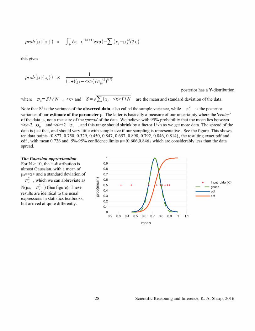
variance of our estimate of the parameter μ. The latter is basically a measure of our uncertainty where the 'center' of the data is, not a measure of the spread of the data. We believe with 95% probability that the mean lies between <x>-2 σμ and <x>+2 σμ , and this range should shrink by a factor 1/√n as we get more data. The spread of the data is just that, and should vary little with sample size if our sampling is representative. See the figure. This shows ten data points {0.877, 0.750, 0.329, 0.450, 0.847, 0.657, 0.898, 0.792, 0.846, 0.814}, the resulting exact pdf and cdf , with mean 0.726 and 5%-95% confidence limits μ={0.606,0.846} which are considerably less than the data spread.

The Gaussian approximationFor N > 10, the 't'-distribution is almost Gaussian, with a mean of μ0=<x> and a standard deviation of σ x

2 , which we can abbreviate as

N(μ0, σ x2 ) (See figure). These

results are identical to the usual expressions in statistics textbooks, but arrived at quite differently.


0.2 0.3 0.4 0.5 0.6 0.7 0.8 0.9 1 1.10

0.1

0.2

0.3

0.4

0.5

0.6

0.7

0.8

0.9

1

Input data {Xi}

gauss

pdf

cdf

mean

pro

b(m

ea

n)

Example 13. Difference between two population meansSee (Sivia and Skilling 2006). Python program: DifferenceInMeans.py

We have two sets of data {xi} i=1, Nx and {yi} i=1, Nx. First we obtain the posterior distributions of the mean of each set, as in the single population case. Using the sample means and sample variances x , S x

2, y , S y2 , the Gaussian

approximation versions of these are

prob (μx |{ x i})≈1

σμ x√2 π

exp[−(μx− x)2/2σμx

2]

prob (μx |{ y i})≈1

σμ y√2 π

exp[−(μ y− x)2/2σμy

2]

where σμ2=S 2

/N is the posterior variance for a single population mean. The joint probability distribution of the two means is, since the two data sets are independent , just the product

prob (μx ,μy |{ xi } ,{ yi })≈1

σμ xσμ y

2πexp (

−12

[(μ x− x )2/2σμ x

2+(μ y− y)2

/2σμy

2])

We want the posterior distribution of the variable 'difference in means', Δμ=μ y−μx Substituting for μy :

prob (Δμ ,μ x |{ x i} ,{ y i})≈1

σμxσμy

2 πexp(

−12

[(μ x− x)2/2σμx

2+(Δμ+μx− y )2

/2σμ y

2])

This is a 2-dimensional pdf. One can remove the dependence on μy by marginalizing over it (integrating with respect to μy), using a constant prior probability prob (μx)=1/constant to obtain (after some tedious algebra!):

prob (Δμ |{ x i} ,{ y i})≈1

σ√2πexp(

−12

[(Δμ−( x− y))2/2σ

2])

where ( x− y) is the difference in sample means and σ2=σμ x

2+σμy

2=S x

2/ N x+S y

2/N y is the

is the posterior variance in our estimate of Δμ. This is conveniently another Gaussian distribution.

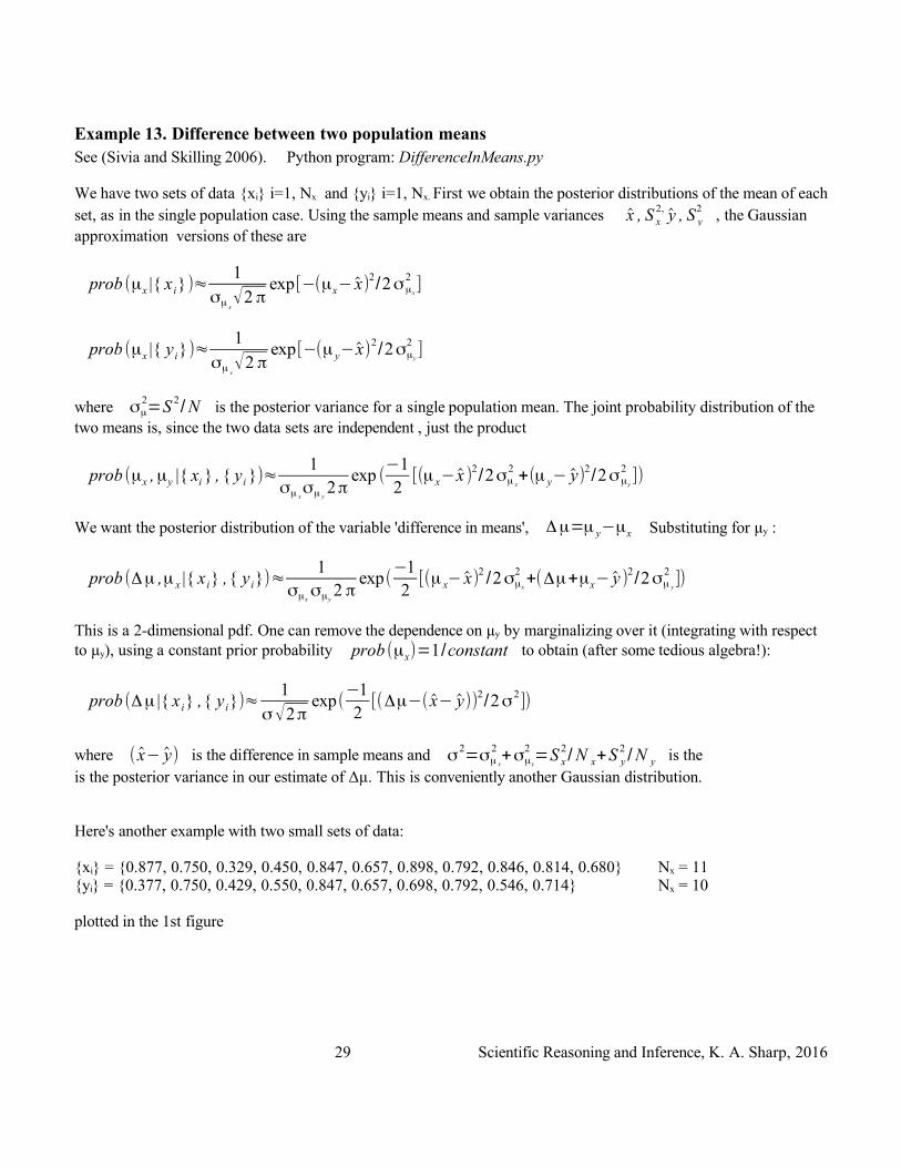
Here's another example with two small sets of data:

{xi} = {0.877, 0.750, 0.329, 0.450, 0.847, 0.657, 0.898, 0.792, 0.846, 0.814, 0.680} Nx = 11{yi} = {0.377, 0.750, 0.429, 0.550, 0.847, 0.657, 0.698, 0.792, 0.546, 0.714} Nx = 10

plotted in the 1st figure


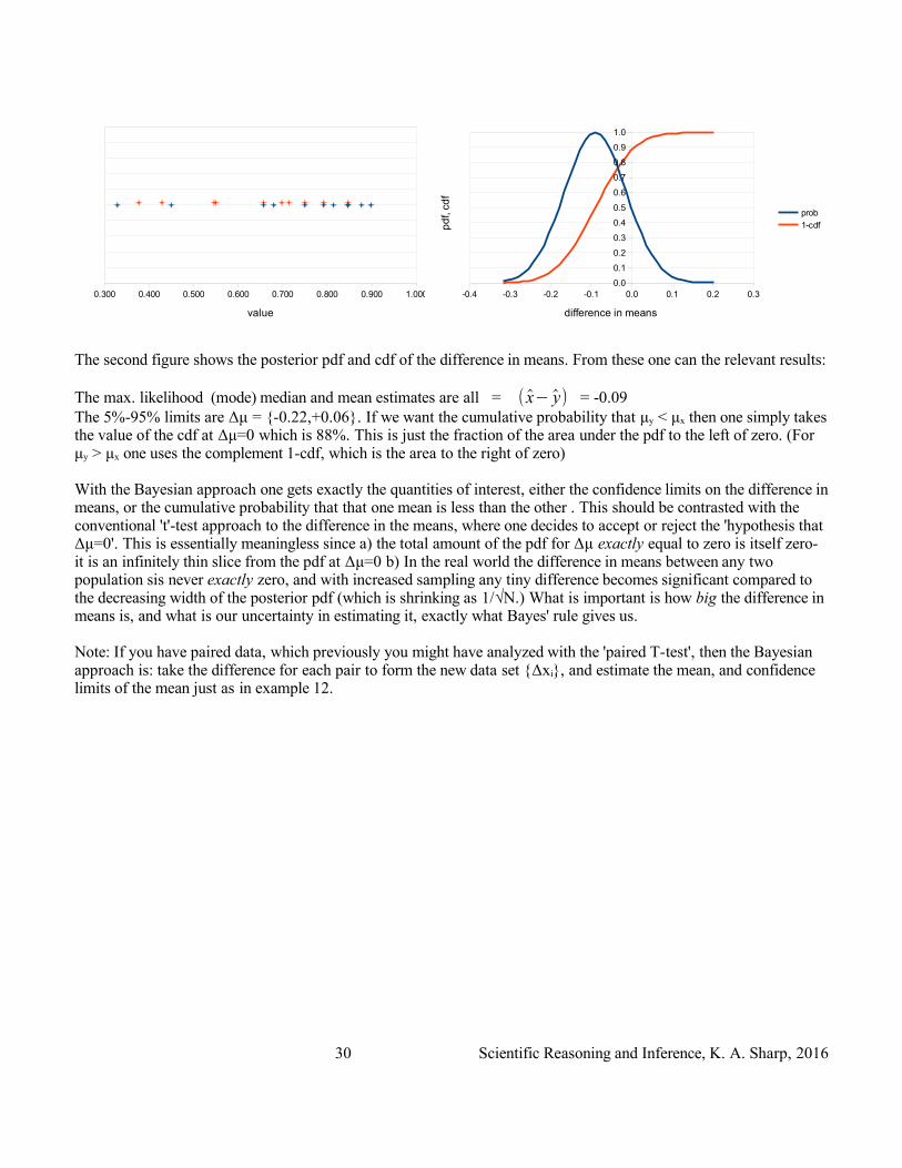
The second figure shows the posterior pdf and cdf of the difference in means. From these one can the relevant results:

The max. likelihood (mode) median and mean estimates are all = ( x− y) = -0.09The 5%-95% limits are Δμ = {-0.22,+0.06}. If we want the cumulative probability that μy < μx then one simply takes the value of the cdf at Δμ=0 which is 88%. This is just the fraction of the area under the pdf to the left of zero. (For μy > μx one uses the complement 1-cdf, which is the area to the right of zero)

With the Bayesian approach one gets exactly the quantities of interest, either the confidence limits on the difference in means, or the cumulative probability that that one mean is less than the other . This should be contrasted with the conventional 't'-test approach to the difference in the means, where one decides to accept or reject the 'hypothesis that Δμ=0'. This is essentially meaningless since a) the total amount of the pdf for Δμ exactly equal to zero is itself zero- it is an infinitely thin slice from the pdf at Δμ=0 b) In the real world the difference in means between any two population sis never exactly zero, and with increased sampling any tiny difference becomes significant compared to the decreasing width of the posterior pdf (which is shrinking as 1/√N.) What is important is how big the difference in means is, and what is our uncertainty in estimating it, exactly what Bayes' rule gives us.

Note: If you have paired data, which previously you might have analyzed with the 'paired T-test', then the Bayesian approach is: take the difference for each pair to form the new data set {Δxi}, and estimate the mean, and confidence limits of the mean just as in example 12.


0.300 0.400 0.500 0.600 0.700 0.800 0.900 1.000

{Xi}

{Yi}

value

-0.4 -0.3 -0.2 -0.1 0.0 0.1 0.2 0.30.0

0.1

0.2

0.3

0.4

0.5

0.6

0.7

0.8

0.9

1.0

prob

1-cdf

difference in means

pd

f, cd

f

More Advanced Applications of Bayes' Rule

Interpretation of probability distribution functions. Part 2The general approach to data analysis and model evaluation using Bayes' rule is to evaluate, either analytically or numerically, the posterior probability of a model or hypothesis H which is specified by parameters a1 , a2 , a3 ... etc. given observed data D, and prior probability prob(H) using

prob (H (a1 , a2 , a3 ...) |D) α prob (D |H (a1 , a2 , a3 ...)) . prob(H (a1 , a2 , a3...))Bayes rule, proportional form

In cases such as parameter estimation, the evidence term is independent of the parameters, and it here it is omitted. The much simpler Bayesian proportionality given above is all we need. Put another way, it results in an un-normalized posterior pdf. In cases where certain parameters a i+1 ...a j are unknown, or 'nuisance' parameters, or we need to evaluate a model without specifying their exact values, these parameters can be marginalized out by integration, and the above becomes

prob(H (a1 ...a i) | D) α prob(H (a1 ...a i)) .

∫δ ai+1...∫ δa j prob (D | H (a1... ai , ai+1... a j)) . prob (ai+ 1) .... prob (a j)Bayes' rule with marginalization of nuisance parameters

where it is assumed that the prior probabilities of the i'th thru j'th parameters are independent. Since the various terms in the above are multiplicative, and resultant probabilities can vary over many orders of magnitude, it is common to work with the logarithm of the posterior probability:

L(a) = log(H(a)|D) + Constant.

Here L(a), often loosely called the log likelihood, is explicitly written as a function of a vector of parameters a = {a1...ai}. The constant absorbs the evidence term and any other factors such as uniform priors that don't depend on a. The estimation of parameters and their confidence intervals then amounts to finding the set of parameter values amax

which maximizes L(a):

∂ L (a)

∂ ai

=0 for all i

and then finding the 'width' of this peak in parameter space. The posterior for the population parameter, example 6, illustrates this for one parameter dimension. If L(a) is a relatively smooth and single-peaked function, it can be well-approximated around its maximum value by a Taylor expansion, which to second order is

L(a)=L(amax)+12∑

i∑

k

∂2 L(a)

∂ ai ∂ ak

|amax(ai−a imax)(ak−ak

max)

where the first derivative terms are all zero at the maximum. Expressing this in a more compact form,

prob (H | D) α exp[12Δ a∇ ∇ L(amax

)Δa ]


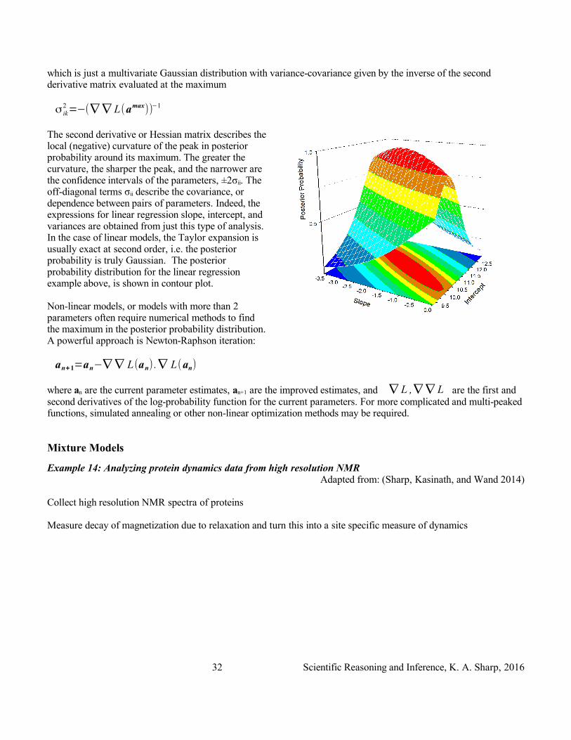
which is just a multivariate Gaussian distribution with variance-covariance given by the inverse of the second derivative matrix evaluated at the maximum

σ ik2 =−(∇ ∇ L(amax))−1

The second derivative or Hessian matrix describes the local (negative) curvature of the peak in posterior probability around its maximum. The greater the curvature, the sharper the peak, and the narrower are the confidence intervals of the parameters, ±2σii. The off-diagonal terms σii describe the covariance, or dependence between pairs of parameters. Indeed, the expressions for linear regression slope, intercept, and variances are obtained from just this type of analysis. In the case of linear models, the Taylor expansion is usually exact at second order, i.e. the posterior probability is truly Gaussian. The posterior probability distribution for the linear regression example above, is shown in contour plot.

Non-linear models, or models with more than 2 parameters often require numerical methods to find the maximum in the posterior probability distribution. A powerful approach is Newton-Raphson iteration:

an+1=an−∇ ∇ L(an) .∇ L(an)

where an are the current parameter estimates, an+1 are the improved estimates, and ∇ L ,∇ ∇ L are the first and second derivatives of the log-probability function for the current parameters. For more complicated and multi-peaked functions, simulated annealing or other non-linear optimization methods may be required.

Mixture Models

Example 14: Analyzing protein dynamics data from high resolution NMRAdapted from: (Sharp, Kasinath, and Wand 2014)

Collect high resolution NMR spectra of proteins

Measure decay of magnetization due to relaxation and turn this into a site specific measure of dynamics


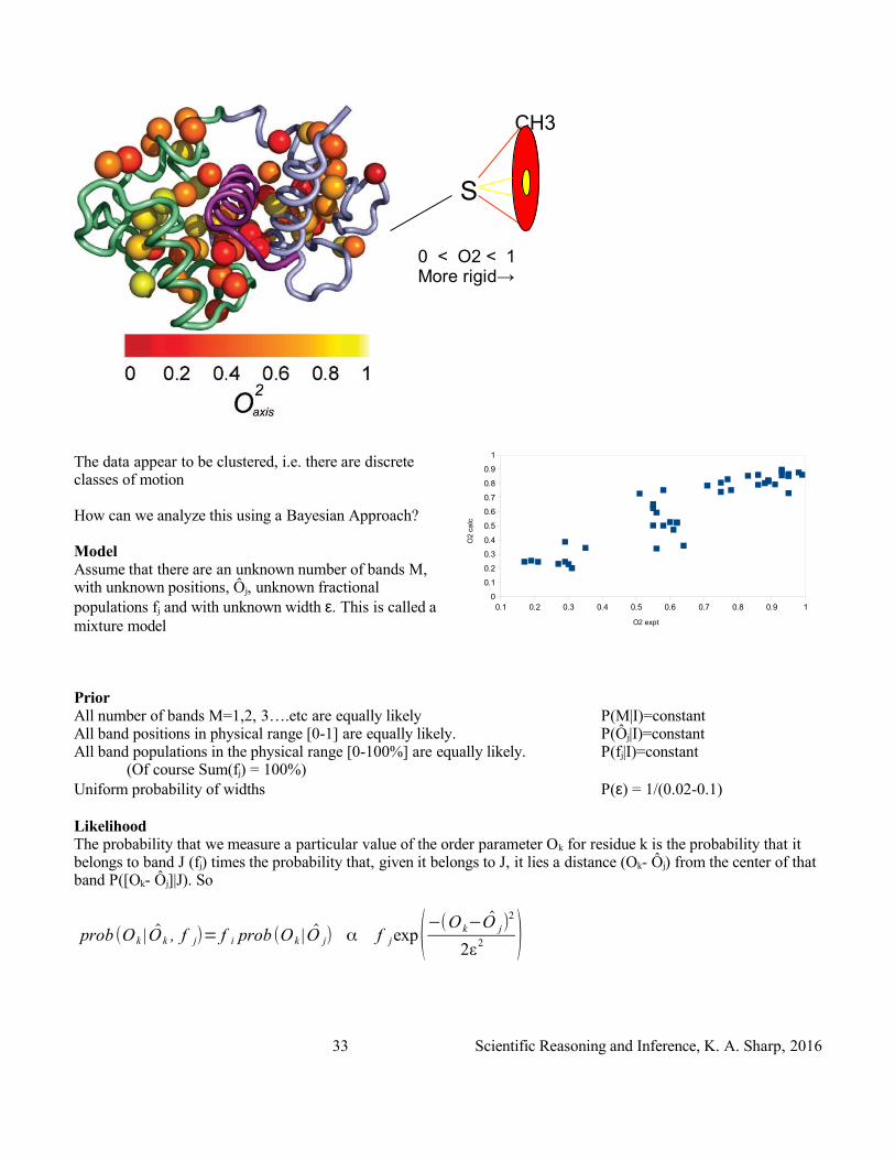
The data appear to be clustered, i.e. there are discrete classes of motion

How can we analyze this using a Bayesian Approach?

ModelAssume that there are an unknown number of bands M, with unknown positions, Ôj, unknown fractional populations fj and with unknown width ε. This is called a mixture model

PriorAll number of bands M=1,2, 3….etc are equally likely P(M|I)=constantAll band positions in physical range [0-1] are equally likely. P(Ôj|I)=constantAll band populations in the physical range [0-100%] are equally likely. P(fj|I)=constant

(Of course Sum(fj) = 100%)Uniform probability of widths P(ε) = 1/(0.02-0.1)

LikelihoodThe probability that we measure a particular value of the order parameter Ok for residue k is the probability that it belongs to band J (fj) times the probability that, given it belongs to J, it lies a distance (Ok- Ôj) from the center of that band P([Ok- Ôj]|J). So

prob (O k |O k , f j)= f i prob (O k |O j) α f jexp(−(O k−O j)2

2ε2 )


CH3

S

0 < O2 < 1More rigid→

0.1 0.2 0.3 0.4 0.5 0.6 0.7 0.8 0.9 10

0.1

0.2

0.3

0.4

0.5

0.6

0.7

0.8

0.9

1

O2 expt

O2

ca

lc

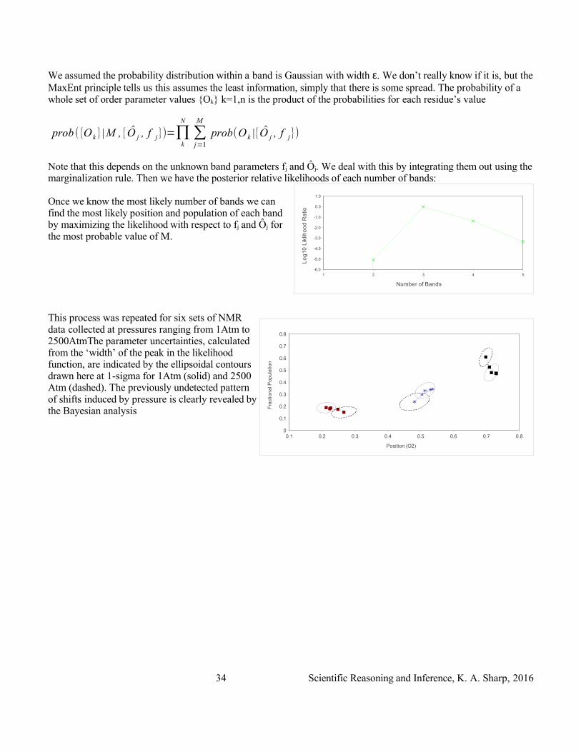
We assumed the probability distribution within a band is Gaussian with width ε. We don’t really know if it is, but the MaxEnt principle tells us this assumes the least information, simply that there is some spread. The probability of a whole set of order parameter values {Ok} k=1,n is the product of the probabilities for each residue’s value

prob ({O k}|M , {O j , f j})=∏k

N

∑j=1

M

prob(O k |{O j , f j})

Note that this depends on the unknown band parameters fj and Ôj. We deal with this by integrating them out using the marginalization rule. Then we have the posterior relative likelihoods of each number of bands:

Once we know the most likely number of bands we can find the most likely position and population of each band by maximizing the likelihood with respect to fj and Ôj for the most probable value of M.

This process was repeated for six sets of NMR data collected at pressures ranging from 1Atm to 2500AtmThe parameter uncertainties, calculated from the ‘width’ of the peak in the likelihood function, are indicated by the ellipsoidal contours drawn here at 1-sigma for 1Atm (solid) and 2500 Atm (dashed). The previously undetected pattern of shifts induced by pressure is clearly revealed by the Bayesian analysis


1 2 3 4 5-6.0

-5.0

-4.0

-3.0

-2.0

-1.0

0.0

1.0

Number of Bands

Lo

g1

0 L

iklih

oo

d R

atio

0.1 0.2 0.3 0.4 0.5 0.6 0.7 0.80

0.1

0.2

0.3

0.4

0.5

0.6

0.7

0.8

Position (O2)

Fra

ctio

na

l Po

pu

latio

n

Example 15. Spectrum analysis and peak detection

Our data is some kind of spectrum, namely the intensity (of absorption, emission, fluorescence, etc) as a function of frequency, I(νi) sampled at N frequencies νi , i=1...N. The model is that the spectrum consists of M bands of amplitude Aj, frequency νj and width (at half maximum height) ωj, j={1...M}. We need a functional form for the line shape of a band: Either a Lorentzian (the theoretical shape for a single absorption band with no inhomogeneous broadening) or more generally a Gaussian. For clarity I'll choose a Lorentzian here, as there are already enough Gaussian functions popping up in the equations! The contribution to the intensity at frequency ν from the j'th Lorentzian band is

I j(ν)=A j ω j

2

(ω j2+(ν−ν j)

2)

and the calculated intensity at frequency νi from all M bands is just the sum of the contributions from each band:

I calc(νi)=∑j=1

M A j ω j2

(ω j2+(νi−ν j)

2)

The model is specified by 3M parameters {Aj, ωj, νj} j={1...M}. The probability of observing the actual data point I(νi) is

prob ( I (νi) | M ,{ A j ,ω j , ν j}) α exp(−( I calc(νi)− I (νi))2

2ϵ2 )

This very general form for the likelihood is known as a Gaussian Noise model, where ε2 is the (possibly unknown) mean squared magnitude of noise. Any kind of contribution to noise is bundled up in ε2 : Thermal, instrument, operator etc.

The probability of observing the entire data set of N intensities forming the spectrum is just the product of the probabilities for each data point:

prob ({ I (νi)}| M ,{ A j ,ω j , ν j }) α Πi=1

Nexp(−( I calc(νi)− I (νi))

2

2ϵ2 ) α exp(−∑i=1

N

δ I i2

2ϵ2 )

where χ2=∑ δ I i

2 is the sum of the square of the 'residuals', the differences between calculated and observed intensity values. Since the likelihood is the product of many probability terms, it is often convenient, both computationally and for human comprehension to work with the log(Likelihood), so

log ( prob({ I (νi)}| M ,{ A j ,ω j , ν j })) = −χ

2(M ,{ A j ,ω j ,ν j})

2ϵ2

+ constant

You may recognize χ2 as the 'goodness of fit' parameter in the conventional 'maximum likelihood' and 'fitting' literature. The Bayesian treatment reveals that it arises from a Gaussian noise model.


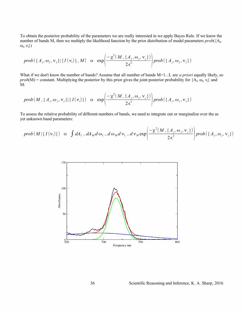
To obtain the posterior probability of the parameters we are really interested in we apply Bayes Rule. If we know the number of bands M, then we multiply the likelihood function by the prior distribution of model parameters prob({Aj, ωj, νj})

prob ({ A j ,ω j ,ν j}| { I (νi)} , M ) α exp(−χ2(M ,{ A j ,ω j , ν j })

2ϵ2 ) prob ({ A j ,ω j ,ν j})

What if we don't know the number of bands? Assume that all number of bands M=1...L are a priori equally likely, so prob(M) = constant. Multiplying the posterior by this prior gives the joint posterior probability for {Aj, ωj, νj} and M:

prob (M ,{ A j ,ω j , ν j }|{ I (νi)}) α exp(−χ2(M ,{ A j ,ω j , ν j })

2ϵ2 ) prob ({ A j ,ω j ,ν j})

To assess the relative probability of different numbers of bands, we need to integrate out or marginalize over the as yet unknown band parameters:

prob (M |{ I (νi)}) α ∫ dA1. ..dAM d ω1. ..d ωM d ν1. .. d νM exp(−χ2(M ,{ A j ,ω j ,ν j })

2ϵ2 ) prob ({ A j ,ω j , ν j})


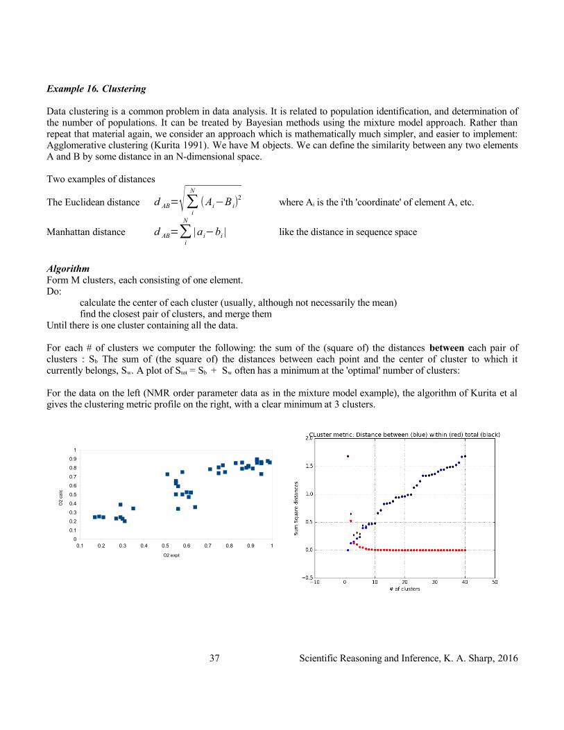
Example 16. Clustering

Data clustering is a common problem in data analysis. It is related to population identification, and determination of the number of populations. It can be treated by Bayesian methods using the mixture model approach. Rather than repeat that material again, we consider an approach which is mathematically much simpler, and easier to implement: Agglomerative clustering (Kurita 1991). We have M objects. We can define the similarity between any two elements A and B by some distance in an N-dimensional space.

Two examples of distances

The Euclidean distance d AB=√∑i

N

(Ai−B i)2

where Ai is the i'th 'coordinate' of element A, etc.

Manhattan distance d AB=∑i

N

|a i−bi | like the distance in sequence space

AlgorithmForm M clusters, each consisting of one element.Do:

calculate the center of each cluster (usually, although not necessarily the mean)find the closest pair of clusters, and merge them

Until there is one cluster containing all the data.

For each # of clusters we computer the following: the sum of the (square of) the distances between each pair of clusters : Sb The sum of (the square of) the distances between each point and the center of cluster to which it currently belongs, Sw. A plot of Stot = Sb + Sw often has a minimum at the 'optimal' number of clusters:

For the data on the left (NMR order parameter data as in the mixture model example), the algorithm of Kurita et al gives the clustering metric profile on the right, with a clear minimum at 3 clusters.


0.1 0.2 0.3 0.4 0.5 0.6 0.7 0.8 0.9 10

0.1

0.2

0.3

0.4

0.5

0.6

0.7

0.8

0.9

1

O2 expt

O2

ca

lc

Estimating rates from counting data. Part 2: Including background countsAdapted from (Loredo 1990) Python program: RareCountsBackgnd.py

First use background counts M over time t to estimate background rate b, just as in counting data example 9 with no background:

prob (b | M , t) α (b t )M exp−bt

M !(gamma distribution)

Then measure counts N over time T with actual sample/source (note N includes both source and background) to estimate source rate s. Applying Bayes rule

prob (s , b | N , M ) α prob( N | s , b) prob (s) prob (b)

prob(s) = constant for s>0, and the prior for b, prob(b), is the posterior obtained from the background counts. The likelihood is given by

prob (N |s , b) α (s+b)N exp−(s+b)T

then the joint posterior for the two rates b and s is

prob (s , b | N , M ) α (s+b)N bM exp−bt exp−(s+b)T

To obtain the posterior for s alone, we integrate over (marginalize out) b

prob (s | N , M ) α ∫0

∞

(s+b)N b M exp−b(t+T )exp−sT db

After some algebra and integration:

prob (s | N , M ) = ∑i=0

NC i T (sT )

i exp− sT/i !

where

C i α (1+tT )

i ( N +M −i) !(N−i)!


Determining a proportion or fraction. Part 2: Using prior informationExample 6, the fraction or probability of a population with some characteristic is examples of determination of a parameter with a physically meaningful range of p={0...1}.

Case 1: No prior data or information. RecapIn the case of the E100M mutation of protein GCB example, we used a uniform prior prob(f) = 1. Then if we have N samples of which M have the characteristic, and N – M don't., the likelihood is

prob ( f | M of N )α prob( M of N | f )=N !

M !(N−M )!f M

(1− f )(M −N ) A beta distribution

fmax = M/N <f> = (M+1)/(N+2) most likely and mean values of proportionσ2 = <f>(1-<f>)/(N+3) variance

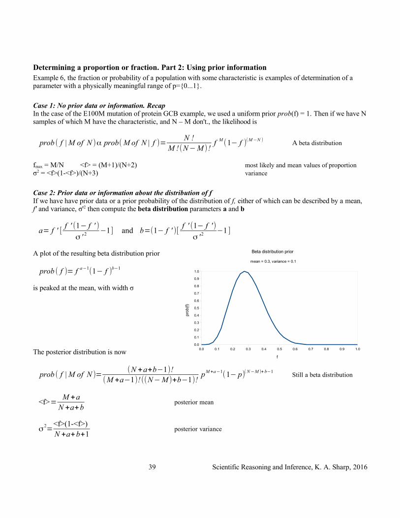
Case 2: Prior data or information about the distribution of fIf we have have prior data or a prior probability of the distribution of f, either of which can be described by a mean, f' and variance, σ'2 then compute the beta distribution parameters a and b

a= f ' [f ' (1− f ' )

σ ' 2 −1] and b=(1− f ' )[f ' (1− f ' )

σ ' 2 −1 ]

A plot of the resulting beta distribution prior

prob ( f )= f a−1(1− f )

b−1

is peaked at the mean, with width σ

The posterior distribution is now

prob ( f | M of N )=(N +a+b−1)!

(M +a−1)! ((N−M )+b−1)!pM +a−1

(1− p)( N −M )+ b−1Still a beta distribution

<f>=M +a

N +a+bposterior mean

σ2=

<f>(1-<f>)N +a+b+1

posterior variance


0.0 0.1 0.2 0.3 0.4 0.5 0.6 0.7 0.8 0.9 1.00.0

0.1

0.2

0.3

0.4

0.5

0.6

0.7

0.8

0.9

1.0

Beta distribution prior

mean = 0.3, variance = 0.1

f

pro

b(f

)

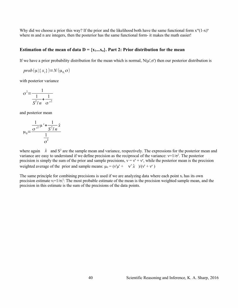
Why did we choose a prior this way? If the prior and the likelihood both have the same functional form xm(1-x)n where m and n are integers, then the posterior has the same functional form- it makes the math easier!

Estimation of the mean of data D = {x1...xn}. Part 2: Prior distribution for the mean

If we have a prior probability distribution for the mean which is normal, N(μ',σ') then our posterior distribution is

prob (μ |{ xi})=N (μ0,σ)

with posterior variance

σ2=

11

S2/ n

+1

σ ' 2

and posterior mean

μ0=

1

σ ' 2 μ ' +1

S 2/ n

x

1

σ2

where again x and S2 are the sample mean and variance, respectively. The expressions for the posterior mean and variance are easy to understand if we define precision as the reciprocal of the variance: ν=1/σ2. The posterior precision is simply the sum of the prior and sample precisions, ν = ν' + νs, while the posterior mean is the precision weighted average of the prior and sample means: μ0 = (ν'μ' + ν

s x )/(ν' + νs )

The same principle for combining precisions is used if we are analyzing data where each point xi has its own precision estimate νi=1/σi

2: The most probable estimate of the mean is the precision weighted sample mean, and the precision in this estimate is the sum of the precisions of the data points.


Bayes' Rule and Scientific Inference

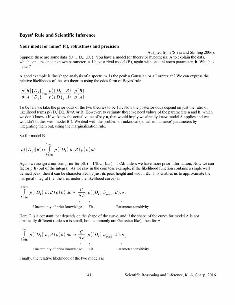
Your model or mine? Fit, robustness and precisionAdapted from (Sivia and Skilling 2006).

Suppose there are some data {D1…Dk…Dn}. You have a model (or theory or hypothesis) A to explain the data, which contains one unknown parameter, a. I have a rival model (B), again with one unknown parameter, b. Which is better?

A good example is line shape analysis of a spectrum. Is the peak a Gaussian or a Lorentzian? We can express the relative likelihoods of the two theories using the odds form of Bayes' rule

p(B∣{ D k })p(A∣{ Dk })

=p({ Dk }∣B)

p({ D}k∣A).

p (B)

p ( A)

To be fair we take the prior odds of the two theories to be 1:1. Now the posterior odds depend on just the ratio of likelihood terms p({Dk}|X), X=A or B. However, to estimate these we need values of the parameters a and b, which we don’t know. (If we knew the actual value of say a, that would imply we already knew model A applies and we wouldn’t bother with model B!). We deal with the problem of unknown (so called nuisance) parameters by integrating them out, using the marginalization rule.

So for model B

p ({Dk }∣B )α ∫b min

b max

p ({Dk }∣b , B ) p( b )db

Again we assign a uniform prior for p(b) = 1/(bmax-bmin) = 1/Δb unless we have more prior information; Now we can factor p(b) out of the integral. As we saw in the coin toss example, if the likelihood function contains a single well defined peak, then it can be characterized by just its peak height and width, σb. This enables us to approximate the marginal integral (i.e. the area under the likelihood curve) as

∫b min

b max

p({Dk }∣b ,B ) p (b ) db ≈CΔ b

. p({Dk }∣b peak , B ). σ b

↑ ↑ ↑Uncertainty of prior knowledge Fit Parameter sensitivity

Here C is a constant that depends on the shape of the curve, and if the shape of the curve for model A is not drastically different (unless n is small, both commonly are Gaussian like), then for A.

∫b min

b max

p({Dk }∣b , A) p( b ) db ≈CΔ a

. p ({Dk }∣a peak , A ). σ a

↑ ↑ ↑Uncertainty of prior knowledge Fit Parameter sensitivity

Finally, the relative likelihood of the two models is


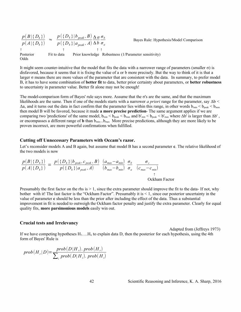
p(B |{ Dk })

p(A |{ Dk })≈

p ({ D k }|b peak , B)

p ({ D k }|a peak , A)

Δ aΔb

σb

σa

Bayes Rule: Hypothesis/Model Comparison

↑ ↑ ↑ ↑Posterior Fit to data Prior knowledge Robustness (1/Parameter sensitivity)Odds

It might seem counter-intuitive that the model that fits the data with a narrower range of parameters (smaller σ) is disfavored, because it seems that it is fixing the value of a or b more precisely. But the way to think of it is that a larger σ means there are more values of the parameter that are consistent with the data. In summary, to prefer model B, it has to have some combination of better fit to data, better prior certainty about parameters, or better robustness to uncertainty in parameter value. Better fit alone may not be enough!

The model-comparison form of Bayes' rule says more. Assume that the σ's are the same, and that the maximum likelihoods are the same. Then if one of the models starts with a narrower a priori range for the parameter, say Δb < Δa, and it turns out the data in fact confirm that the parameter lies within this range, in other words bmin < bpeak < bmax then model B will be favored, because it made a more precise prediction- The same argument applies if we are comparing two 'predictions' of the same model, bmin < bpeak < bmax and b'min < bpeak < b'max where Δb' is larger than Δb' , or encompasses a different range of b than bmin...bmax More precise predictions, although they are more likely to be proven incorrect, are more powerful confirmations when fulfilled.

Cutting off Unnecessary Parameters with Occam’s razor.Let’s reconsider models A and B again, but assume that model B has a second parameter c. The relative likelihood of the two models is now

p(B | { D k })p( A | { D k } )

=p ({ D k }|b peak , c peak , B)

p({ Dk }|a peak , A)

(amax−amin)

(bmax−bmin)

σb

σa

σ c

(cmax−cmin)

↑Ockham Factor

Presumably the first factor on the rhs is > 1, since the extra parameter should improve the fit to the data- If not, why bother with it! The last factor is the “Ockham Factor”. Presumably it is < 1, since our posterior uncertainty in the value of parameter c should be less than the prior after including the effect of the data. Thus a substantial improvement in fit is needed to outweigh the Ockham factor penalty and justify the extra parameter. Clearly for equal quality fits, more parsimonious models easily win out.

Crucial tests and IrrelevancyAdapted from (Jeffreys 1973)

If we have competing hypotheses H1….Hn to explain data D, then the posterior for each hypothesis, using the 4th form of Bayes' Rule is

prob (H r | D)=prob (D |H r) . prob (H r)

∑iprob( D | H i). prob(H i)


If the prior probabilities are comparable, and D has a small probability on all the hypotheses except one, say H1, the prob(H1|D) would be nearly 1. This is referred to as a crucial test.

Conversely, if say prob(D|H1)=1, this implies prob(~D|H1)=0. Now if we observe ~D (not D) then Bayes' rule says prob(H1|~D) = 0. The failure of a crucial test leads to rejection of the hypothesis.

If prob(D|Hi) is the same for all i then the new data don't help us decide between competing hypotheses, so are irrelevant.

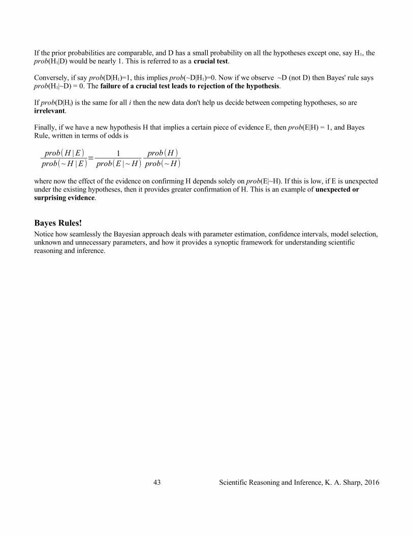
Finally, if we have a new hypothesis H that implies a certain piece of evidence E, then prob(E|H) = 1, and Bayes Rule, written in terms of odds is

prob(H | E )

prob(~ H | E )=

1prob(E | ~ H )

prob (H )

prob(~ H )

where now the effect of the evidence on confirming H depends solely on prob(E|~H). If this is low, if E is unexpected under the existing hypotheses, then it provides greater confirmation of H. This is an example of unexpected or surprising evidence.

Bayes Rules!Notice how seamlessly the Bayesian approach deals with parameter estimation, confidence intervals, model selection, unknown and unnecessary parameters, and how it provides a synoptic framework for understanding scientific reasoning and inference.


ReferencesDewney, Allen. 2012. Think Bayes. 1.08. Green Tea Press.Gull, S. 1988. “Bayesian Inductive Inference and Maximum Entropy.” Max. Ent. and Bayesian Meth. Sci. Eng. 1:

53–74.Howson, Colin., and Peter Urbach. 2006. Scientific Reasoning : The Bayesian Approach  . 3rd ed. Chicago: Open

Court.Iversen, Gudmund R. 1984. Bayesian Statistical Inference. Vol. 43. Quantitative Applications in the Social

Sciences. Beverly Hills: Sage Publications.Jeffreys, Harold. 1973. Scientific Inference. 3d ed. Cambridge [Eng.]: Cambridge University Press.Kurita, Takio. 1991. “An Efficient Agglomerative Clustering Algorithm Using a Heap.” Pattern Recognition 24 (3):

205–9. doi:10.1016/0031-3203(91)90062-A.Loredo, Thomas J. 1990. “From Laplace to Supernova SN 1987A: Bayesian Inference in Astrophysics.” In

Maximum Entropy and Bayesian Methods, 81–142. Springer.Ma, Zhengyu, Kim A. Sharp, Paul A. Janmey, and Terri H. Finkel. 2008. “Surface-Anchored Monomeric Agonist

pMHCs Alone Trigger TCR with High Sensitivity.” PLoS Biology 6: 328–42.MacKay, David J. C. 2003. Information Theory, Inference, and Learning Algorithms. Cambridge, U.K.: Cambridge

University Press.Mendenhall, W., and R. L. Scheaffer. 1973. Mathematical Statistics with Applications. North Scituate, Ma:

Duxbury Press.Scheres, Sjors H.W. 2012. “A Bayesian View on Cryo-EM Structure Determination.” Journal of Molecular Biology

415 (2): 406–18. doi:10.1016/j.jmb.2011.11.010.Sharp, Kim A., Vignesh Kasinath, and A. Joshua Wand. 2014. “Banding of NMR-Derived Methyl Order

Parameters: Implications for Protein Dynamics.” Proteins: Structure, Function, and Bioinformatics, 2106–17. doi:10.1002/prot.24566.

Sivia, D., and J. Skilling. 2006. Data Analysis, a Bayesian Tutorial. Oxford Science Publications. Oxford: Oxford University Press.

Sontag, Sherry. 1998. Blind Man’s Bluff : The Untold Story of American Submarine Espionage  . New York: Public Affairs.

Webster, A. J., and Kemp, R. 2013. “Estimating Omission from Searches.” Am. Statistician 67: 82–89.


Scientific Reasoning and Inference: A Bayesian...

Documents

Transcript of Scientific Reasoning and Inference: A Bayesian...