Sciences Water level forecasting through fuzzy logic … level forecasting through fuzzy logic and...

Hydrology and Earth System Sciences, 10, 1–17, 2006www.copernicus.org/EGU/hess/hess/10/1/SRef-ID: 1607-7938/hess/2006-10-1European Geosciences Union

Hydrology andEarth System

Sciences

Water level forecasting through fuzzy logic and artificial neuralnetwork approaches

S. Alvisi1, G. Mascellani1, M. Franchini 1, and A. Bardossy2

1Dipartimento di Ingegneria, Universita degli Studi di Ferrara, Italia2Institut fur Wasserbau, Universitat Stuttgart, Germany

Received: 29 May 2005 – Published in Hydrology and Earth System Sciences Discussions: 22 June 2005Revised: 16 September 2005 – Accepted: 18 December 2005 – Published: 8 February 2006

Abstract. In this study three data-driven water level fore-casting models are presented and discussed. One is basedon the artificial neural networks approach, while the othertwo are based on the Mamdani and the Takagi-Sugeno fuzzylogic approaches, respectively.

All of them are parameterised with reference to floodevents alone, where water levels are higher than a selectedthreshold. The analysis of the three models is performed byusing thesame input and output variables. However, in or-der to evaluate their capability to deal with different levelsof information, two different input sets are considered. Theformer is characterized by significant spatial and time aggre-gated rainfall information, while the latter considers rainfallinformation more distributed in space and time.

The analysis is made with great attention to the reliabil-ity and accuracy of each model, with reference to the Renoriver at Casalecchio di Reno (Bologna, Italy). It is shown thatthe two models based on the fuzzy logic approaches performbetter when the physical phenomena considered are synthe-sised by both a limited number of variables and IF-THENlogic statements, while the ANN approach increases its per-formance when more detailed information is used. As re-gards the reliability aspect, it is shown that the models basedon the fuzzy logic approaches may fail unexpectedly to fore-cast the water levels, in the sense that in the testing phase,some input combinations are not recognised by the rule sys-tem and thus no forecasting is performed. This problem doesnot occur in the ANN approach.

1 Introduction

Water level forecasting is important for environmental pro-tection and flood control since, when flood events occur, re-

Correspondence to:S. Alvisi([email protected])

liable water level forecasts enable the use both of early warn-ing systems to alert the population, and real time control ofhydraulic structures, like diversion, gates, etc., to mitigatethe flood effects. Information on the flood evolution must beprovided with a reasonable lead time to be effective, but thisis not an easy task, particularly when only rainfall data ob-served up to the forecasting time instant are available, with-out any assumption of future rainfall behaviour.

As is well known, the rainfall-runoff transformation pro-cesses leading to the formation of a flood wave and to theconsequent water level evolution in the river, is extremelycomplex being non-linear, time varying and spatially dis-tributed (Singh, 1964; Pilgrim, 1976). A plethora of rainfall-runoff models have been proposed and used in the past (see,for example, Todini, 1988; Franchini and Pacciani, 1991;Singh and Woolisher, 2002, for a general classification andanalysis). Among them, the most widely used for floodforecasting purposes have a conceptual structure with differ-ent levels of physical information (e.g. Stanford WatershedModel IV (Crawford and Linsey, 1966), Sacramento (Bur-nash et al., 1973), TOPMODEL (Beven and Kirby, 1979;Beven et al., 1984; Sivapalan et al., 1987), ARNO (Todini,1996), TOPKAPI (Liu and Todini, 2002)), or a stochasticstructure (typical examples are those based on ARMA and/orARIMA structures – see, for example, Montanari et al., 2000;Toth et al., 2000). There are also examples where the twoapproaches are combined to improve the forecasting perfor-mance (Ferraresi et al., 1990; Todini, 1988).

In the last decade a new type of data-driven models, basedon artificial intelligence and soft computing technique havebeen applied. In particular, Artificial Neural Network (ANN)is one of the most widely used technique in the forecastingfield (e.g. Hsu et al., 1995; Shamseldin, 1997; Thimuralaiahand Deo, 2000). More recently, Fuzzy Logic (FL) (e.g. Hun-decha et al., 2001;Ozelkan and Duckstein, 2001; Chang etal., 2005), Model Trees (e.g. Solomatine and Dulal, 2003)and hybrid systems based on both ANN and FL have also

© 2006 Author(s). This work is licensed under a Creative Commons License.

2 S. Alvisi et al.: Fuzzy logic vs. neural networks for water level forecasting

been used (e.g. See and Openshaw, 1999, 2000; Abrahartand See, 2002).

Most applications based on these models consider the dis-charge as forecasting variable (e.g. Imrie et al., 2000; Daw-son et al., 2002; Moradkhany et al., 2004), probably be-cause of a historical contiguity with the classes of concep-tual and physically based rainfall-runoff models. Such anapproach requires the knowledge of the rating curve in thecross section of interest (i.e. the basin outlet) to parameter-ize the model. However, the knowledge of the water levelis required within the framework of a flood warning systemand thus the rating curve has to be used also to transform theforecasted flows into water levels.

Models based on ANN, FL, etc., and, more in general, alldata-driven models, can be designed to forecast water lev-els directly, given their very nature. For example, Campoloet al. (1999), See and Openshaw (1999), See and Openshaw(2000), Thirumalaiah and Deo (2000), Campolo et al. (2003),Young (2001, 2002), develop models based mainly on ap-plications of the ANN techniques, while Krzysztofowicz(1999, 2001), Krzysztofowicz and Kelly (2000), Krzyszto-fowicz and Herr (2001) develop a Bayesian forecasting sys-tem which produces a short-term probabilistic river levelforecast based on a probabilistic quantitative precipitationforecast.

The possibility of operating directly on the levels does notapply to the conceptual rainfall runoff models, which arebased on the respect of the mass conservation and even lessto the physically based rainfall runoff models, which, beyondthe respect of the mass conservation at each step of the rain-fall runoff transformation, include further equations reflect-ing details on the energy balance. As a consequence, theselatter models can only deal with the flow.

As previously mentioned, the water level is the quantityof interest within the framework of a flood warning system.Furthermore, it frequently happens that a basin is closed by across section where a long series of registered levels is avail-able but, at the same time, the rating curve is unknown. Inthis latter situation, the only models that can be used to per-form a forecast are those of data-driven type directly appliedto the water levels.

Within this framework, an analysis of two data-driven wa-ter level forecasting approaches is developed: one approachis based on artificial neural networks, whereas the other isbased on fuzzy logic. These two models are selected sincethey are similar, that is, both of them create a quantitativein-ner chain of links between input and output quantities with-out explaining/justifying the physical reason of those links.They mimic, in fact, the intuitive human way of relatingcauseswith theireffects.

Several other papers perform comparisons between data-driven/black box models (see, for example, Goswami et al.,2005), usually focusing on model precision both in calibra-tion and validation phase. In this paper the analysis of theselected models is made with great attention to precision, re-

liability and capability to deal with different levels of infor-mation.

Reliability is considered since the abandoning of any phys-ical constraint such as the mass conservation (typical of anydata-driven model) can represent a potential risk of unex-pected failures in the forecasts, outside the calibration phase.

The capability to deal with different levels of informationis also considered since the FL approach links input and out-put through a decomposition based on categories (low, high,etc.) while the ANN approach links input and output througha system of numerical weights. Indeed the two approachescan behave differently when facing an increasing amount ofdetail and for this reason two different input sets are con-sidered in the numerical test: the former is characterizedby significant spatial and time aggregated rainfall informa-tion, while the latter considers rainfall information more dis-tributed in space and time.

The structure of the paper is as follows. The architec-ture of the ANN and FL models is first presented. Sub-sequently, with reference to the Reno river at Casalecchiodi Reno (Bologna, Italy), two different experiments, charac-terised by different levels of information in the input sets, areset up and discussed, highlighting the behaviour and reliabil-ity of the two approaches.

2 Architecture of the ANN and FL models

2.1 The Artificial Neural Network model

Artificial neural networks reproduce the behaviour of thebrain and nervous systems in a simplified computationalform. They are constituted by highly interconnected sim-ple elements, called artificial neurons, which receive infor-mation, elaborate them through mathematical functions andpass them to other artificial neurons. In particular, in multi-layer perceptron feed-forward networks (Rosenblatt, 1958;Hagan et al., 1996), the artificial neurons are organized inlayers: an input layer, one or more hidden layers and an out-put layer. In this study, one hidden layer is considered, sinceit is shown that this type of network can approximate anyfunction (Hornik et al., 1989; Maier and Dandy, 2000).

With reference to a generic three layer feed-forward net-work with np input neurons,nh hidden neurons andno out-put neurons, the input vectorp, consisting ofnp elements,is multiplied by a weight matrixWP (nh×np) generating avector that is summed with a bias vectorbp (nh). In thehidden layer neurons, each element of the vector obtained istransformed using a nonlinear transfer functionfh, thus gen-erating the vectorh (nh):

h = fh (WPp + bp) (1)

The same procedure is repeated in the output layer. Thus, thevectorh is multiplied by a weight matrixWO (no×nh) gen-erating a vector that is summed with a bias vectorbh (no).

Hydrology and Earth System Sciences, 10, 1–17, 2006 www.copernicus.org/EGU/hess/hess/10/1/

S. Alvisi et al.: Fuzzy logic vs. neural networks for water level forecasting 3

In the neurons of the output layer each element of the vectorobtained is transformed using a nonlinear transfer functionfo generating the output vectoro (no):

o = fo (WHh + bh) (2)

In particular, the transfer functionsfh and fo used in thisstudy in the hidden and output layers, respectively, are a hy-perbolic tangent sigmoid transfer function,

f (x) =ex

− e−x

ex + e−x(3)

and a logsigmoid transfer function,

f (x) =1

1 + e−x(4)

wherex is the generic element of the vectorsWPp+bp andWHh+bh. Other different transfer functions were tested,but the attention was focused on functions (3) and (4) sincethey produce better results and show high flexibility with-out increasing model parameterization. In order to avoidthe problem of output signal saturation (Smith, 1993; Hsuet al., 1995;) the input datumpi is standardized in the range[0.05:0.95] through:

pnormi = 0.05+ 0.9

pi − pmin

pmax − pmin(5)

where [pmin, pmax] is the variation range of the input variableconsidered.

In summary, the full definition of an ANN model impliesthe quantification of the number of neurons in the hiddenlayer and the weight values, since the neuron numbers in theinput and output layers are fixed by the numbers of input andoutput variables, respectively.

As regards the neuron number in the hidden layer, it isusually defined by a trial and error procedure, searching forthe lowest number of neurons without penalizing model effi-ciency (Hsu et al., 1995; Zealand et al., 1999; Chiang et al.,2004).

As regards the quantification of the weight values, two dif-ferent algorithms are frequently used to train the model: theLevenberg Marquardt algorithm (Hagan and Menhaj, 1994)and the scaled conjugate gradient algorithm (Moller, 1993).The former algorithm seems to perform better with ANNmodels characterized by few neurons, and thus few weights,while the latter with ANN models characterized by manyneurons, and thus many weights, (Demuth and Beale, 2000).

In order to avoid overfitting and to improve the ANNmodel robustness, an early stopping procedure is used(ASCE, 2000; Demuth and Beale, 2000). In this procedurethree data sets are considered: a training, a validation and atesting set. The first and the second subsets are used to setup the model, the third subset to test it. More in detail, thefirst subset is used for training the model. At each trainingstep, the calibrated model is validated using the second sub-set. While the first training steps are performed, the error

decreases, as it does in the corresponding validation phase.As the model begins to overfit the data, the error in the val-idation phase begins to rise and thus the training procedureis stopped. The artificial neural network model was imple-mented in Matlab environment where both Levenberg Mar-quardt and scaled conjugate gradient training techniques areavailable in the Neural Network Toolbox.

2.2 Fuzzy logic model

A fuzzy logic model (Zadeh, 1973) is a logical-mathematicalprocedure based on a “IF-THEN” rule system that allows forthe reproduction of the human way of thinking in computa-tional form. In general, a fuzzy rule system has four compo-nents:

– fuzzification of the input: process that transforms the“crisp” (traditional) input into a fuzzy input;

– fuzzy rules: IF-THEN logic system that links the inputto the output variables;

– fuzzy inference: process that elaborates and combinesrule outputs;

– defuzzification of the output: process that transformsthe fuzzy output into a crisp output.

The most widespread methodologies for developing fuzzyrule systems are those proposed by Mamdani (1974) andTakagi-Sugeno (1985). The Mamdani method (FL-M) fol-lows exactly the above mentioned scheme, whereas theTakagi-Sugeno method (FL-TS) uses a composite procedurefor fuzzy inference and output defuzzification. In this study,both methods are used for developing two different forecast-ing models.

With reference to the Mamdani method, being thekth crispinput variable defined asak, Ai,j,k its correspondingj thfuzzy input number considered in theith rule andBi,l thelth fuzzy output number relevant to theith rule, the genericMamdani rule(Ri)M is:

(Ri)M :IF a1 is Ai,j,1 AND a2 is Ai,j,2 AND...AND aK is Ai,j,K

THEN Bi,l

(6)

In the algorithm developed in this study, the degree of fulfil-mentνi of theith rule is obtained with the product inferenceprocedure (Larsen, 1980), then the weighted sum combina-tion is used to define the final output membership functionµB generated by the fuzzy rule system for the crisp inputvector(a1, ..., aK) (Bardossy and Duckstein, 1995). Finallythe crisp output numberb is obtained by applying the cen-troid defuzzification method toµB .

With reference to the Takagi-Sugeno method, being thekth crisp input variable defined asak, Ai,j,k its corresponding

www.copernicus.org/EGU/hess/hess/10/1/ Hydrology and Earth System Sciences, 10, 1–17, 2006


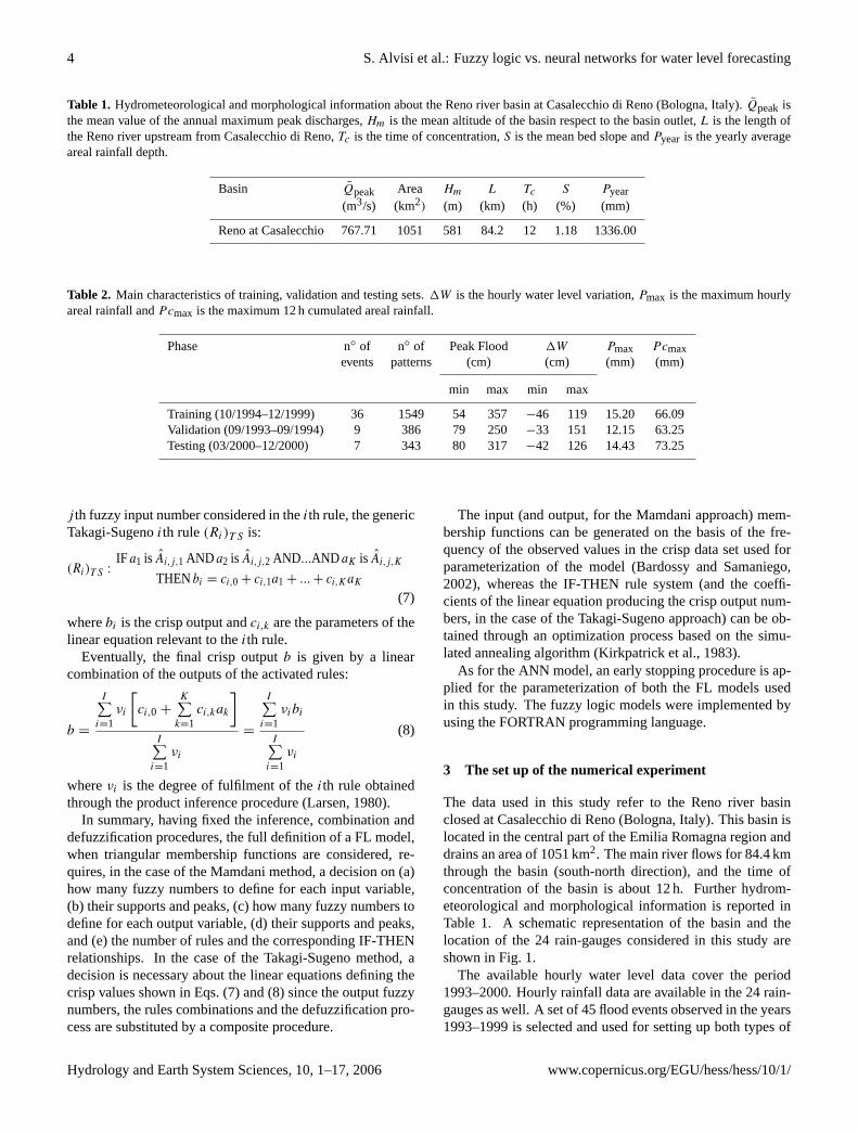
Table 1. Hydrometeorological and morphological information about the Reno river basin at Casalecchio di Reno (Bologna, Italy).Qpeak isthe mean value of the annual maximum peak discharges,Hm is the mean altitude of the basin respect to the basin outlet,L is the length ofthe Reno river upstream from Casalecchio di Reno,Tc is the time of concentration,S is the mean bed slope andPyear is the yearly averageareal rainfall depth.

Basin Qpeak Area Hm L Tc S Pyear

(m3/s) (km2) (m) (km) (h) (%) (mm)

Reno at Casalecchio 767.71 1051 581 84.2 12 1.18 1336.00

Table 2. Main characteristics of training, validation and testing sets.1W is the hourly water level variation,Pmax is the maximum hourlyareal rainfall andPcmax is the maximum 12 h cumulated areal rainfall.

Phase n◦ of n◦ of Peak Flood 1W Pmax Pcmaxevents patterns (cm) (cm) (mm) (mm)

min max min max

Training (10/1994–12/1999) 36 1549 54 357−46 119 15.20 66.09Validation (09/1993–09/1994) 9 386 79 250−33 151 12.15 63.25Testing (03/2000–12/2000) 7 343 80 317−42 126 14.43 73.25

j th fuzzy input number considered in theith rule, the genericTakagi-Sugenoith rule(Ri)T S is:

(Ri)T S :IF a1 is Ai,j,1 AND a2 is Ai,j,2 AND...AND aK is Ai,j,K

THENbi = ci,0 + ci,1a1 + ... + ci,KaK

(7)

wherebi is the crisp output andci,k are the parameters of thelinear equation relevant to theith rule.

Eventually, the final crisp outputb is given by a linearcombination of the outputs of the activated rules:

b =

I∑i=1

νi

[ci,0 +

K∑k=1

ci,kak

]I∑

i=1νi

=

I∑i=1

νibi

I∑i=1

νi

(8)

whereνi is the degree of fulfilment of theith rule obtainedthrough the product inference procedure (Larsen, 1980).

In summary, having fixed the inference, combination anddefuzzification procedures, the full definition of a FL model,when triangular membership functions are considered, re-quires, in the case of the Mamdani method, a decision on (a)how many fuzzy numbers to define for each input variable,(b) their supports and peaks, (c) how many fuzzy numbers todefine for each output variable, (d) their supports and peaks,and (e) the number of rules and the corresponding IF-THENrelationships. In the case of the Takagi-Sugeno method, adecision is necessary about the linear equations defining thecrisp values shown in Eqs. (7) and (8) since the output fuzzynumbers, the rules combinations and the defuzzification pro-cess are substituted by a composite procedure.

The input (and output, for the Mamdani approach) mem-bership functions can be generated on the basis of the fre-quency of the observed values in the crisp data set used forparameterization of the model (Bardossy and Samaniego,2002), whereas the IF-THEN rule system (and the coeffi-cients of the linear equation producing the crisp output num-bers, in the case of the Takagi-Sugeno approach) can be ob-tained through an optimization process based on the simu-lated annealing algorithm (Kirkpatrick et al., 1983).

As for the ANN model, an early stopping procedure is ap-plied for the parameterization of both the FL models usedin this study. The fuzzy logic models were implemented byusing the FORTRAN programming language.

3 The set up of the numerical experiment

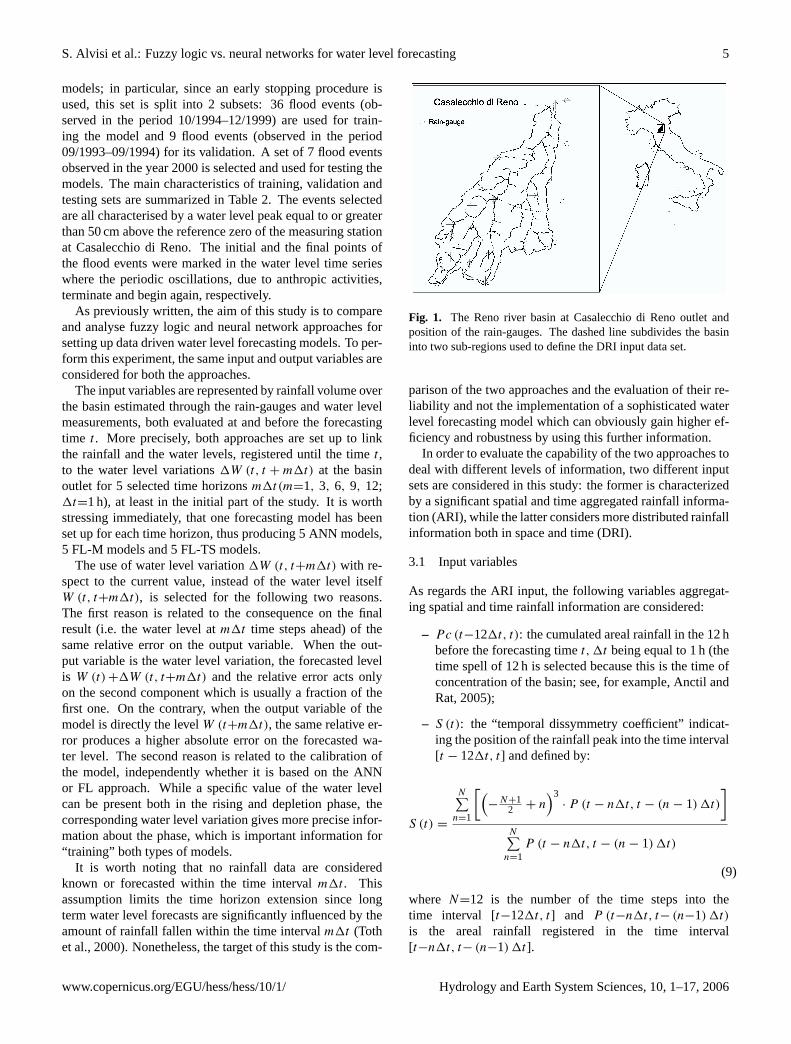
The data used in this study refer to the Reno river basinclosed at Casalecchio di Reno (Bologna, Italy). This basin islocated in the central part of the Emilia Romagna region anddrains an area of 1051 km2. The main river flows for 84.4 kmthrough the basin (south-north direction), and the time ofconcentration of the basin is about 12 h. Further hydrom-eteorological and morphological information is reported inTable 1. A schematic representation of the basin and thelocation of the 24 rain-gauges considered in this study areshown in Fig. 1.

The available hourly water level data cover the period1993–2000. Hourly rainfall data are available in the 24 rain-gauges as well. A set of 45 flood events observed in the years1993–1999 is selected and used for setting up both types of



models; in particular, since an early stopping procedure isused, this set is split into 2 subsets: 36 flood events (ob-served in the period 10/1994–12/1999) are used for train-ing the model and 9 flood events (observed in the period09/1993–09/1994) for its validation. A set of 7 flood eventsobserved in the year 2000 is selected and used for testing themodels. The main characteristics of training, validation andtesting sets are summarized in Table 2. The events selectedare all characterised by a water level peak equal to or greaterthan 50 cm above the reference zero of the measuring stationat Casalecchio di Reno. The initial and the final points ofthe flood events were marked in the water level time serieswhere the periodic oscillations, due to anthropic activities,terminate and begin again, respectively.

As previously written, the aim of this study is to compareand analyse fuzzy logic and neural network approaches forsetting up data driven water level forecasting models. To per-form this experiment, the same input and output variables areconsidered for both the approaches.

The input variables are represented by rainfall volume overthe basin estimated through the rain-gauges and water levelmeasurements, both evaluated at and before the forecastingtime t . More precisely, both approaches are set up to linkthe rainfall and the water levels, registered until the timet ,to the water level variations1W (t, t + m1t) at the basinoutlet for 5 selected time horizonsm1t(m=1, 3, 6, 9, 12;1t=1 h), at least in the initial part of the study. It is worthstressing immediately, that one forecasting model has beenset up for each time horizon, thus producing 5 ANN models,5 FL-M models and 5 FL-TS models.

The use of water level variation1W (t, t+m1t) with re-spect to the current value, instead of the water level itselfW (t, t+m1t), is selected for the following two reasons.The first reason is related to the consequence on the finalresult (i.e. the water level atm1t time steps ahead) of thesame relative error on the output variable. When the out-put variable is the water level variation, the forecasted levelis W (t) +1W (t, t+m1t) and the relative error acts onlyon the second component which is usually a fraction of thefirst one. On the contrary, when the output variable of themodel is directly the levelW (t+m1t), the same relative er-ror produces a higher absolute error on the forecasted wa-ter level. The second reason is related to the calibration ofthe model, independently whether it is based on the ANNor FL approach. While a specific value of the water levelcan be present both in the rising and depletion phase, thecorresponding water level variation gives more precise infor-mation about the phase, which is important information for“training” both types of models.

It is worth noting that no rainfall data are consideredknown or forecasted within the time intervalm1t . Thisassumption limits the time horizon extension since longterm water level forecasts are significantly influenced by theamount of rainfall fallen within the time intervalm1t (Tothet al., 2000). Nonetheless, the target of this study is the com-

Fig. 1. The Reno river basin at Casalecchio di Reno outlet andposition of the rain-gauges. The dashed line subdivides the basininto two sub-regions used to define the DRI input data set.

parison of the two approaches and the evaluation of their re-liability and not the implementation of a sophisticated waterlevel forecasting model which can obviously gain higher ef-ficiency and robustness by using this further information.

In order to evaluate the capability of the two approaches todeal with different levels of information, two different inputsets are considered in this study: the former is characterizedby a significant spatial and time aggregated rainfall informa-tion (ARI), while the latter considers more distributed rainfallinformation both in space and time (DRI).

3.1 Input variables

As regards the ARI input, the following variables aggregat-ing spatial and time rainfall information are considered:

– Pc (t−121t, t): the cumulated areal rainfall in the 12 hbefore the forecasting timet, 1t being equal to 1 h (thetime spell of 12 h is selected because this is the time ofconcentration of the basin; see, for example, Anctil andRat, 2005);

– S (t): the “temporal dissymmetry coefficient” indicat-ing the position of the rainfall peak into the time interval[t − 121t, t ] and defined by:

S (t) =

N∑n=1

[(−

N+12 + n

)3· P (t − n1t, t − (n − 1) 1t)

]N∑

n=1P (t − n1t, t − (n − 1) 1t)

(9)

where N=12 is the number of the time steps into thetime interval [t−121t, t ] and P (t−n1t, t− (n−1) 1t)

is the areal rainfall registered in the time interval[t−n1t, t− (n−1) 1t ].



1 3 6 9 120

10

20

30

40

50

RM

SE

[cm

]

hours ahead

a)

FL-M

FL-TS

ANN

FL-M E.S.

FL-TS E.S.

ANN E.S.

1 3 6 9 120

10

20

30

40

50

RM

SE

[cm

]

hours ahead

b)

FL-M

FL-TS

ANNFL-M E.S.

FL-TS E.S.

ANN E.S.

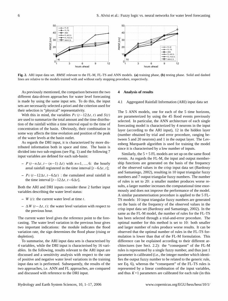
Fig. 2. ARI input data set.RMSErelevant to the FL-M, FL-TS and ANN models.(a) training phase,(b) testing phase. Solid and dashedlines are relative to the models trained with and without early stopping procedure, respectively.

As previously mentioned, the comparison between the twodifferent data-driven approaches for water level forecastingis made by using the same input sets. To do this, the inputsets are necessarily selected a priori and the criterion used fortheir selection is “physical” representativity.

With this in mind, the variablesPc (t−121t, t) andS(t)

are used to summarize the total amount and the time distribu-tion of the rainfall within a time interval equal to the time ofconcentration of the basin. Obviously, their combination insome way affects the time evolution and position of the peakof the water levels at the basin outlet.

As regards the DRI input, it is characterized by more dis-tributed information both in space and time. The basin isdivided into two sub-regions (see Fig. 1) and the following 7input variables are defined for each sub-basin:

– P (t−n1t, t− (n−1)1t) with n=1, ..., 6: the hourlyareal rainfall registered in the time interval[t−61t, t ];

– Pc (t−121t, t−61t) : the cumulated areal rainfall inthe time interval[t−121t, t−61t ].

Both the ARI and DRI inputs consider these 2 further inputvariables describing the water level status:

– W (t): the current water level at timet .

– 1W (t−1t, t): the water level variation with respect tothe previous hour.

The current water level gives the reference point to the fore-casting. The water level variation in the previous hour givestwo important indications: the module indicates the floodvariation rate, the sign determines the flood phase (rising ordepletion).

To summarise, the ARI input data sets is characterised by4 variables, while the DRI input is characterised by 16 vari-ables. In the following, results relevant to the ARI input arediscussed and a sensitivity analysis with respect to the rateof positive and negative water level variations in the traininginput data set is performed. Subsequently, the results of thetwo approaches, i.e. ANN and FL approaches, are comparedand discussed with reference to the DRI input.

4 Analysis of results

4.1 Aggregated Rainfall Information (ARI) input data set

The 5 ANN models, one for each of the 5 time horizons,are parameterized by using the 45 flood events previouslyselected. In particular, the ANN architecture of each singleforecasting model is characterized by 4 neurons in the inputlayer (according to the ARI input), 12 in the hidden layer(number obtained by trial and error procedure, ranging be-tween 5 and 20 neurons) and 1 in the output layer. The Lev-enberg Marquardt algorithm is used for training the modelsince it is characterised by a low number of inputs.

Similarly, the 5 + 5 FL models are set up on the same floodevents. As regards the FL-M, the input and output member-ship functions are generated on the basis of the frequencyof the observed values in the crisp input data set (Bardossyand Samaniego, 2002), resulting in 10 input triangular fuzzynumbers and 7 output triangular fuzzy numbers. The numberof rules is set to 20: a smaller number produces worse re-sults, a larger number increases the computational time enor-mously and does not improve the performance of the model.A similar parameterisation procedure is applied to the 5 FL-TS models: 10 input triangular fuzzy numbers are generatedon the basis of the frequency of the observed values in thecrisp input data set (Bardossy and Samaniego, 2002). In thesame as the FL-M model, the number of rules for the FL-TShas been selected through a trial-and-error procedure. Theoptimal number for this method is set to 10: both smallerand larger number of rules produce worse results. It can beobserved that the optimal number of rules in the FL-TS for-mulation is lower than that of the FL-M formulation. Thisdifference can be explained according to their different ar-chitectures (see Sect. 2.2): the “consequent” of the FL-Mrules is represented by a single fuzzy number, and thus just 1parameter is calibrated (i.e., the integer number which identi-fies the output fuzzy number to be related to the generic rule,see Eq. 6), whereas the “consequent” of the FL-TS rules isrepresented by a linear combination of the input variables,and thusK+1 parameters are calibrated for each rule (in this



1 3 6 9 120

0.2

0.4

0.6

0.8

1

R2

hours ahead

a)

FL-MFL-TSANN

1 3 6 9 120

0.2

0.4

0.6

0.8

1

R2

hours ahead

b)

FL-MFL-TSANN

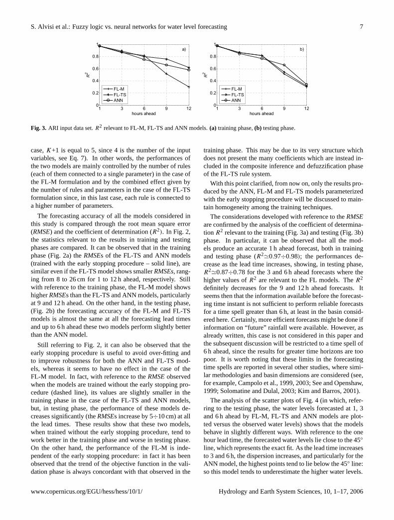
Fig. 3. ARI input data set.R2 relevant to FL-M, FL-TS and ANN models.(a) training phase,(b) testing phase.

case,K+1 is equal to 5, since 4 is the number of the inputvariables, see Eq. 7). In other words, the performances ofthe two models are mainly controlled by the number of rules(each of them connected to a single parameter) in the case ofthe FL-M formulation and by the combined effect given bythe number of rules and parameters in the case of the FL-TSformulation since, in this last case, each rule is connected toa higher number of parameters.

The forecasting accuracy of all the models considered inthis study is compared through the root mean square error(RMSE) and the coefficient of determination (R2). In Fig. 2,the statistics relevant to the results in training and testingphases are compared. It can be observed that in the trainingphase (Fig. 2a) theRMSEs of the FL-TS and ANN models(trained with the early stopping procedure – solid line), aresimilar even if the FL-TS model shows smallerRMSEs, rang-ing from 8 to 26 cm for 1 to 12 h ahead, respectively. Stillwith reference to the training phase, the FL-M model showshigherRMSEs than the FL-TS and ANN models, particularlyat 9 and 12 h ahead. On the other hand, in the testing phase,(Fig. 2b) the forecasting accuracy of the FL-M and FL-TSmodels is almost the same at all the forecasting lead timesand up to 6 h ahead these two models perform slightly betterthan the ANN model.

Still referring to Fig. 2, it can also be observed that theearly stopping procedure is useful to avoid over-fitting andto improve robustness for both the ANN and FL-TS mod-els, whereas it seems to have no effect in the case of theFL-M model. In fact, with reference to theRMSEobservedwhen the models are trained without the early stopping pro-cedure (dashed line), its values are slightly smaller in thetraining phase in the case of the FL-TS and ANN models,but, in testing phase, the performance of these models de-creases significantly (theRMSEs increase by 5÷10 cm) at allthe lead times. These results show that these two models,when trained without the early stopping procedure, tend towork better in the training phase and worse in testing phase.On the other hand, the performance of the FL-M is inde-pendent of the early stopping procedure: in fact it has beenobserved that the trend of the objective function in the vali-dation phase is always concordant with that observed in the

training phase. This may be due to its very structure whichdoes not present the many coefficients which are instead in-cluded in the composite inference and defuzzification phaseof the FL-TS rule system.

With this point clarified, from now on, only the results pro-duced by the ANN, FL-M and FL-TS models parameterizedwith the early stopping procedure will be discussed to main-tain homogeneity among the training techniques.

The considerations developed with reference to theRMSEare confirmed by the analysis of the coefficient of determina-tion R2 relevant to the training (Fig. 3a) and testing (Fig. 3b)phase. In particular, it can be observed that all the mod-els produce an accurate 1 h ahead forecast, both in trainingand testing phase (R2

'0.97÷0.98); the performances de-crease as the lead time increases, showing, in testing phase,R2

'0.87÷0.78 for the 3 and 6 h ahead forecasts where thehigher values ofR2 are relevant to the FL models. TheR2

definitely decreases for the 9 and 12 h ahead forecasts. Itseems then that the information available before the forecast-ing time instant is not sufficient to perform reliable forecastsfor a time spell greater than 6 h, at least in the basin consid-ered here. Certainly, more efficient forecasts might be done ifinformation on “future” rainfall were available. However, asalready written, this case is not considered in this paper andthe subsequent discussion will be restricted to a time spell of6 h ahead, since the results for greater time horizons are toopoor. It is worth noting that these limits in the forecastingtime spells are reported in several other studies, where simi-lar methodologies and basin dimensions are considered (see,for example, Campolo et al., 1999, 2003; See and Openshaw,1999; Solomatine and Dulal, 2003; Kim and Barros, 2001).

The analysis of the scatter plots of Fig. 4 (in which, refer-ring to the testing phase, the water levels forecasted at 1, 3and 6 h ahead by FL-M, FL-TS and ANN models are plot-ted versus the observed water levels) shows that the modelsbehave in slightly different ways. With reference to the onehour lead time, the forecasted water levels lie close to the 45◦

line, which represents the exact fit. As the lead time increasesto 3 and 6 h, the dispersion increases, and particularly for theANN model, the highest points tend to lie below the 45◦ line:so this model tends to underestimate the higher water levels.



Fig. 4. ARI input data set – testing phase. Water levels forecasted at 1, 3 and 6 h ahead (rows 1, 2 and 3, respectively) by the FL-M, FL-TSand ANN models (columns 1, 2 and 3, respectively) versus the observed data.

0 10 20 30 40 50 60 70 800

50

100

150

200

wat

er le

vel [

cm]

t [h]

a)

0 10 20 30 40 50 60 70 800

50

100

150

200

wat

er le

vel [

cm]

t [h]

b)

0 10 20 30 40 50 60 70 800

50

100

150

200

wat

er le

vel [

cm]

t [h]

c)

Fig. 5. ARI input data set – testing phase. Ensemble of the water levels forecasted at 1, 3 and 6 h ahead starting from each hour of the floodevent considered.(a) FL-M model,(b) FL-TS model,(c) ANN model.

To compare the models in more detail, an event of thetesting set is shown in Fig. 5 where the 1, 3 and 6 h aheadforecasts, calculated at each time step, are plotted. In thisspecific event, the FL-M, FL-TS and ANN models show a

similar behaviour: in all the cases the greatest differencesbetween observed and forecasted water levels occur in therising part of the wave, where a marked underestimation isobserved. The similar behaviour of the FL-M, FL-TS and



0 10 20 30 40 50 60 70 80 900

50

100

150

200

t [h]w

ater

leve

l [cm

] a) ObservedFL-MFL-TSANN

0 10 20 30 40 50 60 70 80 900

50

100

150

200

t [h]

wat

er le

vel [

cm] b) Observed

FL-MFL-TSANN

0 10 20 30 40 50 60 70 80 900

50

100

150

200

t [h]

wat

er le

vel [

cm] c) Observed

FL-MFL-TSANN

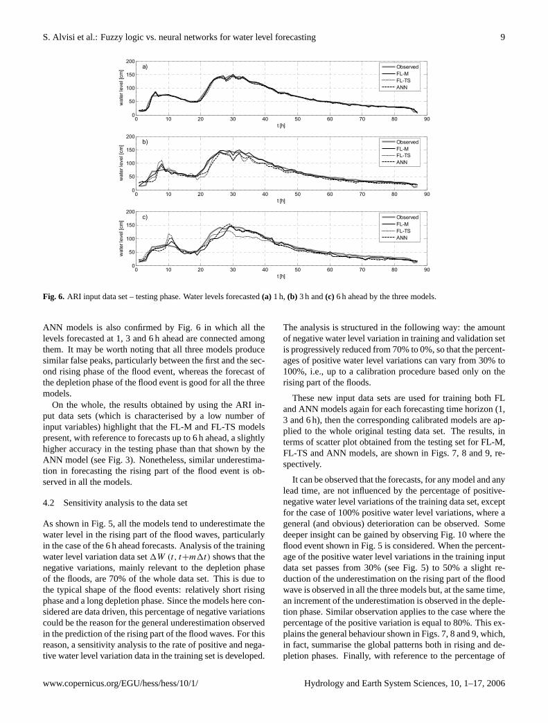
Fig. 6. ARI input data set – testing phase. Water levels forecasted(a) 1 h, (b) 3 h and(c) 6 h ahead by the three models.

ANN models is also confirmed by Fig. 6 in which all thelevels forecasted at 1, 3 and 6 h ahead are connected amongthem. It may be worth noting that all three models producesimilar false peaks, particularly between the first and the sec-ond rising phase of the flood event, whereas the forecast ofthe depletion phase of the flood event is good for all the threemodels.

On the whole, the results obtained by using the ARI in-put data sets (which is characterised by a low number ofinput variables) highlight that the FL-M and FL-TS modelspresent, with reference to forecasts up to 6 h ahead, a slightlyhigher accuracy in the testing phase than that shown by theANN model (see Fig. 3). Nonetheless, similar underestima-tion in forecasting the rising part of the flood event is ob-served in all the models.

4.2 Sensitivity analysis to the data set

As shown in Fig. 5, all the models tend to underestimate thewater level in the rising part of the flood waves, particularlyin the case of the 6 h ahead forecasts. Analysis of the trainingwater level variation data set1W (t, t+m1t) shows that thenegative variations, mainly relevant to the depletion phaseof the floods, are 70% of the whole data set. This is due tothe typical shape of the flood events: relatively short risingphase and a long depletion phase. Since the models here con-sidered are data driven, this percentage of negative variationscould be the reason for the general underestimation observedin the prediction of the rising part of the flood waves. For thisreason, a sensitivity analysis to the rate of positive and nega-tive water level variation data in the training set is developed.

The analysis is structured in the following way: the amountof negative water level variation in training and validation setis progressively reduced from 70% to 0%, so that the percent-ages of positive water level variations can vary from 30% to100%, i.e., up to a calibration procedure based only on therising part of the floods.

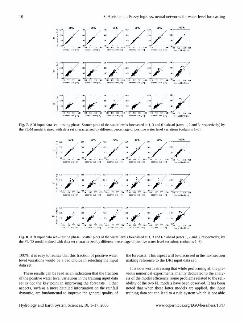
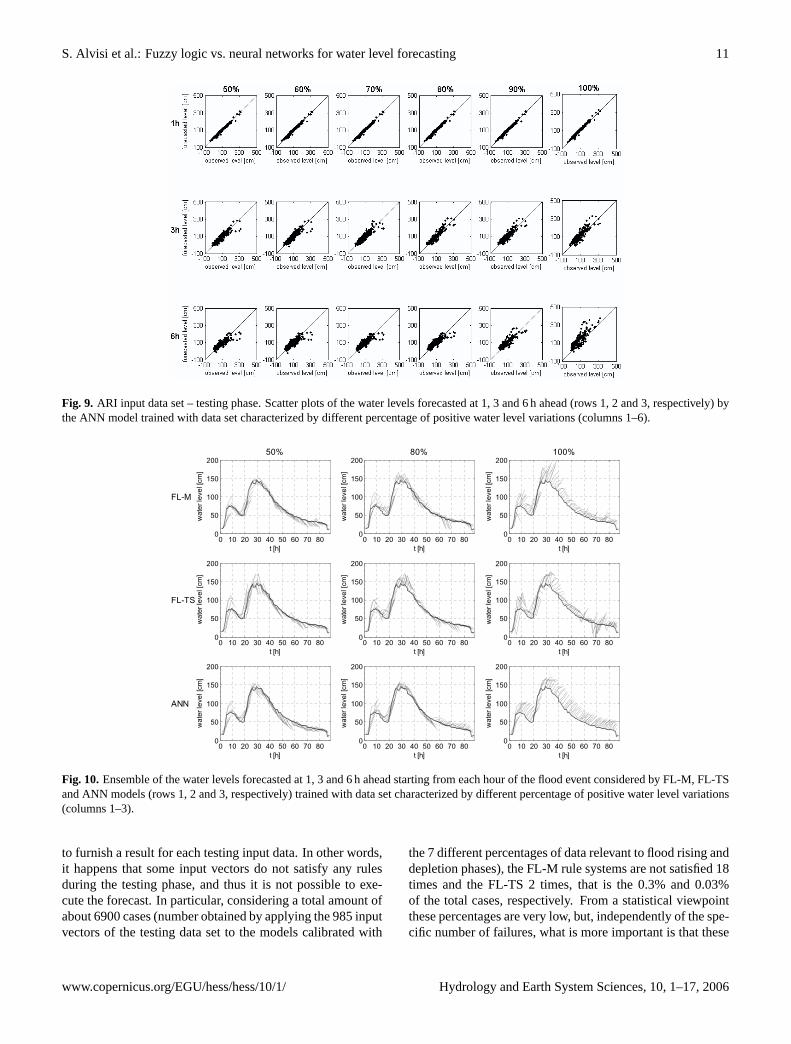
These new input data sets are used for training both FLand ANN models again for each forecasting time horizon (1,3 and 6 h), then the corresponding calibrated models are ap-plied to the whole original testing data set. The results, interms of scatter plot obtained from the testing set for FL-M,FL-TS and ANN models, are shown in Figs. 7, 8 and 9, re-spectively.

It can be observed that the forecasts, for any model and anylead time, are not influenced by the percentage of positive-negative water level variations of the training data set, exceptfor the case of 100% positive water level variations, where ageneral (and obvious) deterioration can be observed. Somedeeper insight can be gained by observing Fig. 10 where theflood event shown in Fig. 5 is considered. When the percent-age of the positive water level variations in the training inputdata set passes from 30% (see Fig. 5) to 50% a slight re-duction of the underestimation on the rising part of the floodwave is observed in all the three models but, at the same time,an increment of the underestimation is observed in the deple-tion phase. Similar observation applies to the case where thepercentage of the positive variation is equal to 80%. This ex-plains the general behaviour shown in Figs. 7, 8 and 9, which,in fact, summarise the global patterns both in rising and de-pletion phases. Finally, with reference to the percentage of



Fig. 7. ARI input data set – testing phase. Scatter plots of the water levels forecasted at 1, 3 and 6 h ahead (rows 1, 2 and 3, respectively) bythe FL-M model trained with data set characterized by different percentage of positive water level variations (columns 1–6).

Fig. 8. ARI input data set – testing phase. Scatter plots of the water levels forecasted at 1, 3 and 6 h ahead (rows 1, 2 and 3, respectively) bythe FL-TS model trained with data set characterized by different percentage of positive water level variations (columns 1–6).

100%, it is easy to realize that this fraction of positive waterlevel variations would be a bad choice in selecting the inputdata set.

These results can be read as an indication that the fractionof the positive water level variations in the training input dataset is not the key point in improving the forecasts. Otheraspects, such as a more detailed information on the rainfalldynamic, are fundamental to improve the general quality of

the forecasts. This aspect will be discussed in the next sectionmaking reference to the DRI input data set.

It is now worth stressing that while performing all the pre-vious numerical experiments, mainly dedicated to the analy-sis of the model efficiency, some problems related to the reli-ability of the two FL models have been observed. It has beennoted that when these latter models are applied, the inputtraining data set can lead to a rule system which is not able



Fig. 9. ARI input data set – testing phase. Scatter plots of the water levels forecasted at 1, 3 and 6 h ahead (rows 1, 2 and 3, respectively) bythe ANN model trained with data set characterized by different percentage of positive water level variations (columns 1–6).

0 10 20 30 40 50 60 70 800

50

100

150

200

wat

er le

vel [

cm]

t [h]

50%

FL-M

0 10 20 30 40 50 60 70 800

50

100

150

200

wat

er le

vel [

cm]

t [h]

FL-TS

0 10 20 30 40 50 60 70 800

50

100

150

200

wat

er le

vel [

cm]

t [h]

ANN

0 10 20 30 40 50 60 70 800

50

100

150

200

wat

er le

vel [

cm]

t [h]

80%

0 10 20 30 40 50 60 70 800

50

100

150

200

wat

er le

vel [

cm]

t [h]

0 10 20 30 40 50 60 70 800

50

100

150

200

wat

er le

vel [

cm]

t [h]

0 10 20 30 40 50 60 70 800

50

100

150

200

wat

er le

vel [

cm]

t [h]

100%

0 10 20 30 40 50 60 70 800

50

100

150

200

wat

er le

vel [

cm]

t [h]

0 10 20 30 40 50 60 70 800

50

100

150

200

wat

er le

vel [

cm]

t [h]

Fig. 10.Ensemble of the water levels forecasted at 1, 3 and 6 h ahead starting from each hour of the flood event considered by FL-M, FL-TSand ANN models (rows 1, 2 and 3, respectively) trained with data set characterized by different percentage of positive water level variations(columns 1–3).

to furnish a result for each testing input data. In other words,it happens that some input vectors do not satisfy any rulesduring the testing phase, and thus it is not possible to exe-cute the forecast. In particular, considering a total amount ofabout 6900 cases (number obtained by applying the 985 inputvectors of the testing data set to the models calibrated with

the 7 different percentages of data relevant to flood rising anddepletion phases), the FL-M rule systems are not satisfied 18times and the FL-TS 2 times, that is the 0.3% and 0.03%of the total cases, respectively. From a statistical viewpointthese percentages are very low, but, independently of the spe-cific number of failures, what is more important is that these



1 3 60

10

20

30

40

50

RM

SE

[cm

]

hours ahead

a)

FL-MFL-TSANN

1 3 60

10

20

30

40

50

RM

SE

[cm

]

hours ahead

b)

FL-MFL-TSANN

1 3 60

0.2

0.4

0.6

0.8

1

R2

hours ahead

c)

FL-MFL-TSANN

1 3 60

0.2

0.4

0.6

0.8

1

R2

hours ahead

d)

FL-MFL-TSANN

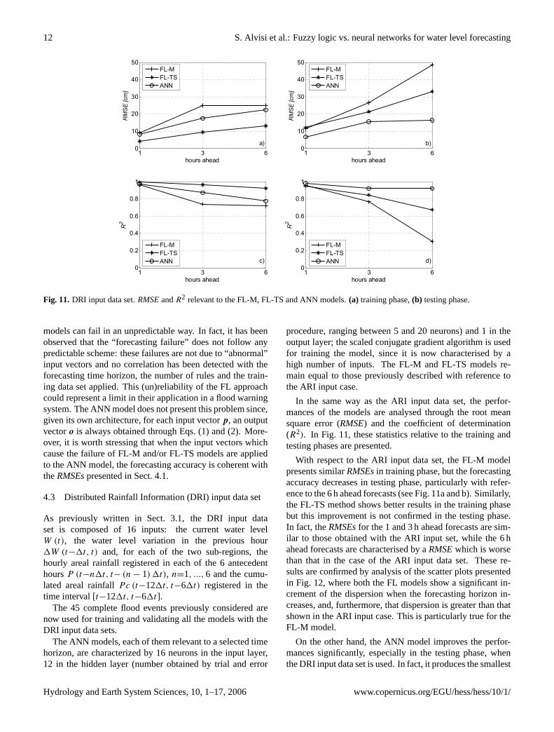
Fig. 11. DRI input data set.RMSEandR2 relevant to the FL-M, FL-TS and ANN models.(a) training phase,(b) testing phase.

models can fail in an unpredictable way. In fact, it has beenobserved that the “forecasting failure” does not follow anypredictable scheme: these failures are not due to “abnormal”input vectors and no correlation has been detected with theforecasting time horizon, the number of rules and the train-ing data set applied. This (un)reliability of the FL approachcould represent a limit in their application in a flood warningsystem. The ANN model does not present this problem since,given its own architecture, for each input vectorp, an outputvectoro is always obtained through Eqs. (1) and (2). More-over, it is worth stressing that when the input vectors whichcause the failure of FL-M and/or FL-TS models are appliedto the ANN model, the forecasting accuracy is coherent withtheRMSEspresented in Sect. 4.1.

4.3 Distributed Rainfall Information (DRI) input data set

As previously written in Sect. 3.1, the DRI input dataset is composed of 16 inputs: the current water levelW (t), the water level variation in the previous hour1W (t−1t, t) and, for each of the two sub-regions, thehourly areal rainfall registered in each of the 6 antecedenthoursP (t−n1t, t− (n − 1) 1t), n=1, ..., 6 and the cumu-lated areal rainfallPc (t−121t, t−61t) registered in thetime interval[t−121t, t−61t ].

The 45 complete flood events previously considered arenow used for training and validating all the models with theDRI input data sets.

The ANN models, each of them relevant to a selected timehorizon, are characterized by 16 neurons in the input layer,12 in the hidden layer (number obtained by trial and error

procedure, ranging between 5 and 20 neurons) and 1 in theoutput layer; the scaled conjugate gradient algorithm is usedfor training the model, since it is now characterised by ahigh number of inputs. The FL-M and FL-TS models re-main equal to those previously described with reference tothe ARI input case.

In the same way as the ARI input data set, the perfor-mances of the models are analysed through the root meansquare error (RMSE) and the coefficient of determination(R2). In Fig. 11, these statistics relative to the training andtesting phases are presented.

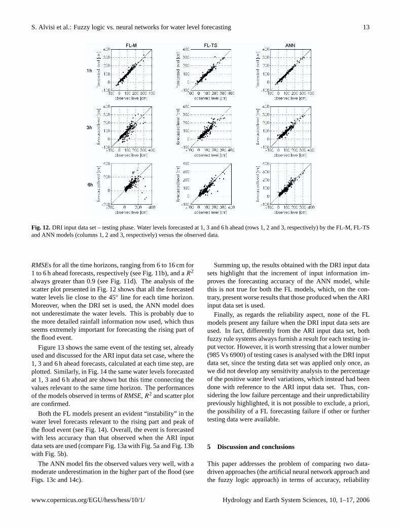
With respect to the ARI input data set, the FL-M modelpresents similarRMSEsin training phase, but the forecastingaccuracy decreases in testing phase, particularly with refer-ence to the 6 h ahead forecasts (see Fig. 11a and b). Similarly,the FL-TS method shows better results in the training phasebut this improvement is not confirmed in the testing phase.In fact, theRMSEsfor the 1 and 3 h ahead forecasts are sim-ilar to those obtained with the ARI input set, while the 6 hahead forecasts are characterised by aRMSEwhich is worsethan that in the case of the ARI input data set. These re-sults are confirmed by analysis of the scatter plots presentedin Fig. 12, where both the FL models show a significant in-crement of the dispersion when the forecasting horizon in-creases, and, furthermore, that dispersion is greater than thatshown in the ARI input case. This is particularly true for theFL-M model.

On the other hand, the ANN model improves the perfor-mances significantly, especially in the testing phase, whenthe DRI input data set is used. In fact, it produces the smallest



Fig. 12. DRI input data set – testing phase. Water levels forecasted at 1, 3 and 6 h ahead (rows 1, 2 and 3, respectively) by the FL-M, FL-TSand ANN models (columns 1, 2 and 3, respectively) versus the observed data.

RMSEs for all the time horizons, ranging from 6 to 16 cm for1 to 6 h ahead forecasts, respectively (see Fig. 11b), and aR2

always greater than 0.9 (see Fig. 11d). The analysis of thescatter plot presented in Fig. 12 shows that all the forecastedwater levels lie close to the 45◦ line for each time horizon.Moreover, when the DRI set is used, the ANN model doesnot underestimate the water levels. This is probably due tothe more detailed rainfall information now used, which thusseems extremely important for forecasting the rising part ofthe flood event.

Figure 13 shows the same event of the testing set, alreadyused and discussed for the ARI input data set case, where the1, 3 and 6 h ahead forecasts, calculated at each time step, areplotted. Similarly, in Fig. 14 the same water levels forecastedat 1, 3 and 6 h ahead are shown but this time connecting thevalues relevant to the same time horizon. The performancesof the models observed in terms ofRMSE, R2 and scatter plotare confirmed.

Both the FL models present an evident “instability” in thewater level forecasts relevant to the rising part and peak ofthe flood event (see Fig. 14). Overall, the event is forecastedwith less accuracy than that observed when the ARI inputdata sets are used (compare Fig. 13a with Fig. 5a and Fig. 13bwith Fig. 5b).

The ANN model fits the observed values very well, with amoderate underestimation in the higher part of the flood (seeFigs. 13c and 14c).

Summing up, the results obtained with the DRI input datasets highlight that the increment of input information im-proves the forecasting accuracy of the ANN model, whilethis is not true for both the FL models, which, on the con-trary, present worse results that those produced when the ARIinput data set is used.

Finally, as regards the reliability aspect, none of the FLmodels present any failure when the DRI input data sets areused. In fact, differently from the ARI input data set, bothfuzzy rule systems always furnish a result for each testing in-put vector. However, it is worth stressing that a lower number(985 Vs 6900) of testing cases is analysed with the DRI inputdata set, since the testing data set was applied only once, aswe did not develop any sensitivity analysis to the percentageof the positive water level variations, which instead had beendone with reference to the ARI input data set. Thus, con-sidering the low failure percentage and their unpredictabilitypreviously highlighted, it is not possible to exclude, a priori,the possibility of a FL forecasting failure if other or furthertesting data were available.

5 Discussion and conclusions

This paper addresses the problem of comparing two data-driven approaches (the artificial neural network approach andthe fuzzy logic approach) in terms of accuracy, reliability



0 10 20 30 40 50 60 70 800

50

100

150

200

wat

er le

vel [

cm]

t [h]

a)

0 10 20 30 40 50 60 70 800

50

100

150

200

wat

er le

vel [

cm]

t [h]

b)

0 10 20 30 40 50 60 70 800

50

100

150

200

wat

er le

vel [

cm]

t [h]

c)

Fig. 13.DRI input data set – testing phase. Ensemble of the water levels forecasted at 1, 3 and 6 h ahead starting from each hour of the floodevent considered.(a) FL-M model,(b) FL-TS model,(c) ANN model.

0 10 20 30 40 50 60 70 80 900

50

100

150

200

t [h]

wat

er le

vel [

cm] a) Observed

FL-MFL-TSANN

0 10 20 30 40 50 60 70 80 900

50

100

150

200

t [h]

wat

er le

vel [

cm] b) Observed

FL-MFL-TSANN

0 10 20 30 40 50 60 70 80 900

50

100

150

200

t [h]

wat

er le

vel [

cm] c) Observed

FL-MFL-TSANN

Fig. 14. DRI input data set – testing phase. Water levels forecasted(a) 1 h, (b) 3 h and(c) 6 h ahead by the three models.

and capability of dealing with different levels of information,within the framework of a water level forecasting system.

As regards the accuracy, all the models provide good ac-curacy for short time horizon forecasts which however de-creases when longer time horizons are considered and this isparticularly true for the rising phase of the flood wave where

a systematic underestimation is observed when the modelsare trained with the ARI input data set. A lead time up to 6 hahead can be however considered acceptable for both FL andANN approaches. This temporal limit is coherent with thatdetected by other authors using similar data-driven modelsapplied to basins with similar extension to that considered in



this study (e.g. Campolo et al., 1999, 2003; See and Open-shaw, 1999; Solomatine and Dulal, 2003), and this limit iscertainly due to the fact that no information or forecast ofrainfall is considered available within the time spell aheadwith respect to the time instant when the forecast is per-formed.

The analysis of the model accuracy, when the ARI inputdata set is used, shows that, overall, the FL-M and FL-TSmodels perform slightly better than the ANN model in termsof RMSEsandR2. However, as previously recalled, all themodels underestimate the water levels in the rising part of theflood waves and this can be related to the little informationon rainfall dynamic available in the ARI input data set.

As regards the reliability, it has been shown that the mod-els considered present a different level of reliability. Boththe FL models produce some unexpected failure. In partic-ular, they are not able to execute a forecast in some testingcases since the input vectors do not satisfy any “IF” condi-tion of the trained/calibrated rules. This lack of response cansuggest that the FL approach is certainly appropriate whenthe enumeration of all the possibilities can be done a priori,as in the case of some mechanical or electronic tool, but itmay not be totally reliable when dealing with natural phe-nomenon where the number of possible combinations maybe extremely large and where input combinations not con-sidered in the training phase can produce no results. TheANN model does not present this problem since, given itsown architecture, for each input vector an output vector isalways obtained through the transfer functions of the hiddenand output layers.

As regards the capability to deal with different level of in-formation, the use of the DRI input data set highlights furtherdifferences between the FL and ANN approaches. The ANNaccuracy increases significantly and, at the same time, thetendency to underestimate the future water levels decreasessignificantly with respect to that observed in the case of theARI input data set. This behaviour indicates that the greaterdetail in the rainfall pattern is useful to forecast the water lev-els more accurately, especially in the rising part of the floodevents.

As regards the FL-M and FL-TS models, the forecastingaccuracy in the testing phase does not increase, or becomeseven worse when the DRI input data set are used. This in-dicates that the FL approach, independently of its formula-tion, has a limited capability of dealing with too detailed in-formation, and this result is in line with other hydrologicalstudies based on fuzzy rules system which, in fact, are gen-erally characterized by a low number (from 2 to 5) of inputvariables (see, for example, Abebe et al., 2000; Hundechaet al., 2001; Xiong et al., 2001; Han et al., 2002; Changet al., 2005). A similar limit exists also for the number ofrules that can be implemented within the framework of aFL model. It has in fact been shown that the accuracy ofthe model initially increases with the number of rules, butbeyond a certain number, the accuracy of the model starts

to decrease again. All these latter considerations show that,given their very structure, the FL approaches perform betterwhen the physical phenomena considered are synthesised byboth a limited number of variables and IF-THEN logic state-ments, while the ANN approach increases its performancewhen more detailed information is used.

Overall, both approaches may be used within the frame-work of a real time forecasting system, though with differ-ent levels of reliability. Both of them however show per-formances which remain satisfactory up to 6 h ahead for thebasin considered, which indeed is too short for operationalflood forecasting. While it is worth stressing that the aim ofthis paper was the comparison between the two approacheswithin the terms recalled at the beginning of this section, thislatter observation highlights the need to feed these modelswith further information, with respect to the time of fore-casting, relevant to the future rainfall amount and its spatialand time distribution. This further information should ar-rive mainly from radar data, possibly elaborated by anothermodel dedicated to the rainfall forecast, which would allowthe time spell of prediction to be extended to useful opera-tional time intervals.

Finally, we can observe that the models here considered,for their very nature, are “blind” with respect to specificphysical information: they only deal with data (e.g. rainfalland levels) which indirectly contain the “integral” behaviourof the system to be modelled. As a consequence, since thecomparison presented was performed with reference to abasin of a humid region, it is expected that similar results(in terms of comparison between the two approaches) canbe obtained when other basins located in similar regionsare considered. On the contrary, if basins located in dryregions were considered, different inputs and structures maybe selected and identified, so the relative performances ofthe two models may change. Further analyses are currentlybeing developed with reference to catchments in dry regionsto analyse these latter aspects.

Edited by: E. Todini

References

Abebe, A. J., Solomatine, D. P., and Venneker, R. G. W.: Appli-cation of adaptive fuzzy rule-based models for reconstructionof missing precipitation events, Hydrol. Sci. J., 45(3), 425–436,2000.

Abrahart, R. J. and See, L.: Multi-model data fusion for river flowforecasting: an evaluation of six alternative methods based ontwo contrasting catchments, Hydrol. Earth Syst. Sci., 6, 655–670,2002,SRef-ID: 1607-7938/hess/2002-6-655.

Anctil, F. and Rat, A.: Evaluation of Neural Network Streamflowforecasting on 47 Watershed, J. Hydrol. Eng., 10(1), 85–88,2005.


http://direct.sref.org/1607-7938/hess/2002-6-655


ASCE Task Committee on the application of ANN in Hydrology:Artificial Neural Networks in Hydrology. I: Preliminary Con-cepts, J. Hydrol. Eng., 5(2), 115–123, 2000.

Bardossy, A. and Duckstein, L.: Fuzzy rule-based modelling withapplications to geophysical, Biological and Engineering Sys-tems, CRC Press, Boca Raton, Florida, 1995.

Bardossy, A. and Samaniego, L.: Fuzzy Rule-Based Classificationof Remotely Sensed Imagery, IEEE Transactions on Geosciencesand Remote Sensing, 40, 362–374, 2002.

Beven, K. J. and Kirby, M. J.: A physically based variable con-tributing area model of basin hydrology, Hydrol. Sci. Bull., 24,1–3, 1979.

Beven, K. J., Kirby, M. J., Schofield, N., and Tagg, A. F.: Testinga physically-based flood forecasting model (TOPMODEL) forthree U.K. catchments, J. Hydrol., 69, 119–143, 1984.

Burnash, R. J. C., Ferrel, R. L., and Mc Guire, R. A.: A generalStreamflow Simulation System – Conceptual Modelling for Dig-ital Computers, Report by the Joint Federal State River ForecastCenter, Sacramento, 1973.

Campolo, M., Andreussi, P., and Soldati, A.: River flood forecast-ing with neural network model, Water Resour. Res., 35(4), 1191–1197, 1999.

Campolo, M., Andreussi, P., and Soldati, A.: Artificial neural net-work approach to flood forecasting in the river Arno, Hydrol. Sci.J., 48(3), 381-398, 2003.

Chang, L. C., Chang, F. J., and Tsai, Y. H.: Fuzzy exemplar-basedinference system for flood forecasting, Water Resour. Res., 41,W02005, doi:10.1029/2004WR003037, 2005.

Chiang, Y. M., Chang, L. C., and Chang, F. J.: Comparison of static-feedforward and dynamic-feedback neural network for rainfall-runoff modelling, J. Hydrol., 290, 297–311, 2004.

Crawford, N. H. and Linsey, R. K.: Digital simulation in hydrology,Stanford Watershed Model IV. Tech. Rep. No. 39, Dep. Civ. Eng.,Stanford University, 1966.

Dawson, C. W., Harpham, C., Wilby, R. L., and Chen, Y.: Evalua-tion of artificial neural network technique in the River Yangtze,China, Hydrol. Earth Syst. Sci., 6, 619–626, 2002,SRef-ID: 1607-7938/hess/2002-6-619.

Demuth, H. B. and Beale, M.: Neural Network Toolbox for use withMatlab, The Math Works, Inc., Natick, 2000.

Ferraresi, M., Pacciani, M., and Todini, E.: Sull’applicazione dialcuni schemi di previsione di piena fluviale in tempo reale, Attidel XXII convegno di Idraulica e Costruzioni Idrauliche, 3, 307–320, 1990.

Franchini, M. and Pacciani, M.: Comparative analysis of severalconceptual rainfall-runoff models, J. Hydrol., 122, 161–219,1991.

Goswami, M., O’Connor, K. M., Bhattarai, K. P., and Shamseldin,A. Y.: Assessing the performance of eight real-time updatingmodels and procedures for the Brosna River, Hydrol. Earth Syst.Sci., 9, 394–411, 2005,SRef-ID: 1607-7938/hess/2005-9-394.

Hagan, M. T., Demuth, H. B., and Beale, M.: Neural Network De-sign, PWS Publishing Company, Boston, 1996.

Hagan, M. T. and Menhaj, M.: Training feedforward networks withthe Marquardt algorithm, IEEE Transaction on Neural Networks,5(6), 989–993, 1994.

Han, D., Cluckie, I. D., Karbassioun, D., Lawry, J., and Krauskopf,B.: River Flow Modelling using Fuzzy Decision Trees, Water

Resour. Manag., 16, 431–445, 2002.Hornik, K., Stinchombe, M., and White, H.: Multilayer feedfor-

ward networks are universal approximators, Neural Networks, 2,359–366, 1989.

Hsu, K. L., Gupta, H. V., and Sorooshian, S.: Artificial neural net-work modeling of the rainfall-runoff process, Water Resour. Res.,31(10), 2517–2530, 1995.

Hundecha, Y., Bardossy, A., and Theisen, H. W.: Development ofa fuzzy logic-based rainfall-runoff model, Hydrol. Sci. J., 46(3),363–376, 2001.

Imrie, C. E., Durucan, S., and Korre, A.: River flow prediction usingartificial neural networks: generalizations beyond the calibrationrange, J. Hydrol., 233, 138–153, 2000.

Kim, G. and Barros, A. P.: Quantitative flood forecasting using mul-tisensor data and neural networks, J. Hydrol., 246, 45–62, 2001.

Kirkpatrick, S., Gelat Jr., C. D., and Vecchi, M. P.: Optimization bysimulated annealing, Science, 220(4598), 671–680, 1983.

Krzysztofowicz, R.: Bayesian theory of probabilistic forecastingvia deterministic hydrologic model, Water Resour. Res., 35(9),2739–2750, 1999.

Krzysztofowicz, R. and Kelly, K. S.: Hydrologic uncertainty pro-cessor for probabilistic river stage Forecasting, Water Resour.Res., 36(11), 3265–3277, 2000.

Krzysztofowicz, R. and Herr, H. D.: Hydrologic uncertainty pro-cessor for probabilistic river stage forecasting: precipitation-dependent model, J. Hydrol., 249, 46–68, 2001.

Krzysztofowicz, R.: Integrator of uncertainties for probabilisticriver stage forecasting: precipitation-dependent model, J. Hy-drol. 249, 69–85, 2001.

Larsen, P. M.: Industrial applications of Fuzzy Logic Control, Int.J. Man Mach. Stud., 12(1), 3–10, 1980.

Liu, Z. and Todini, E.: Towards a comprehensive physically basedrainfall-runoff model, Hydrol. Earth Syst. Sci., 6, 859–881, 2002,SRef-ID: 1607-7938/hess/2002-6-859.

Maier, H. R. and Dandy, G. C.: Neural Networks for predictionand forecasting of water resources variables: a review of mod-elling issue and applications, Environmental Modelling & Soft-ware, 15, 101–124, 2000.

Mamdani, E. H.: Application of Fuzzy Algorithm for Control ofSimple Dynamic Plant, Proc. IEEE, 121, 1585–1888, 1974.

Moller, M. F.: A scaled conjugate gradient algorithm for fast super-vised learning, Neural Networks, 6, 525–533, 1993.

Montanari, A., Rosso, R., and Taqqu, M. S.: A seasonal frac-tional ARIMA model applied to the Nile River monthly flowsat Aswan, Water Resour. Res., 36(5), 1249–1259, 2000.

Moradkhany, H., Hsu, K. L., Gupta, H. V., and Sorooshian, S.: Im-proved streamflow forecasting using self-organizing radial-basisfunction artificial neural networks, J. Hydrol., 295, 246–262,2004.

Ozelkan, E. C. and Duckstein, L.: Fuzzy conceptual rainfall-runoffmodels, J. Hydrol., 253, 41–68, 2001.

Pilgrim, D. H.: Travel times and non linearity of flood runoff fromtracer measurements on a small watershed, Water Resour. Res.,12(3), 487–496, 1976.

Rosenblatt, F.: The Perceptron: A probabilistic model for informa-tion storage and organization in the brain, Psycological Review,65, 386–408, 1958.

See, L. and Openshaw, S.: Applying soft computing approaches toriver level forecasting, Hydrol. Sci. J., 44(5), 763–778, 1999.






See, L. and Openshaw, S.: A hybrid multi-model approach to riverlevel forecasting, Hydrol. Sci. J., 45(4), 523–536, 2000.

Shamseldin, A. Y.: Application of a neural network technique torainfall-runoff modelling, J. Hydrol., 199, 272–294, 1997.

Singh, V. P.: Non linear instantaneous unit hydrograph theory, J.Hydraul. Div. Am. Soc. Civ. Eng., 90(HY2), 313–347, 1964.

Singh, V. P. and Woolhiser, D. A.: Mathematical Modeling of Wa-tershed Hydrology, J. Hydrol. Eng., 7(4), 270–292, 2002.

Sivapalan, M., Beven, K. J., and Wood, K. F.: On Hydrologicalsimilarity 2. A scaled model of storm runoff production, WaterResour. Res., 23, 2266–2278, 1987.

Smith, M.: Neural Network for statistical modelling, Van NostrandRehinold, New York, 1993.

Solomatine, D. P. and Dulal, K. N.: Model trees as an alternativeto neural networks in rainfall runoff modelling, Hydrol. Sci. J.,48(3), 399–411, 2003.

Takagi, T. and Sugeno, M.: Fuzzy identification of systems andits application to modelling and control, IEEE Transactions onSystems, Man, and Cybernetics, 15(1), 116–132, 1985.

Thimuralaiah, K. and Deo, M. C.: Hydrological forecasting UsingNeural Networks, J. Hydrol. Eng., 5(2), 180–189, 2000.

Toth, E., Brath, A., and Montanari, A.: Comparison of short-termrainfall prediction models for real-time flood forecasting, J. Hy-drol., 239, 132–147, 2000.

Todini, E.: Rainfall-Runoff modeling – Past, present and future, J.Hydrol., 100, 341–352, 1988.

Todini, E.: The ARNO rainfall-runoff model, J. Hydrol., 175, 339–382, 1996.

Xiong, L., Shamseldin, A. Y., and O’Connor, K. M.: A non-linearcombination of the forecasts of rainfall-runoff models by thefirst-order Takagi-Sugeno fuzzy system, J. Hydrol., 245, 196–217, 2001.

Young, P C.: Data-based mechanistic modelling and validation ofrainfall-flow processes, in: Model Validation: Perspectives inHydrological Science, edited by: Anderson, M. G. and Bates,P. D., Wiley, Chichester, pp. 117–161, 2001.

Young, P. C.: Advances in real-time flood forecasting, Philosoph-ical Transactions of the Royal Society: Mathematical, Physicaland Engineering Sciences, 2002.

Zadeh, L. A.: The concept of a linguistic variable and its applicationto approximate reasoning, Memorandum ERL-M 411, Berkeley,1973.

Zealand, C. M., Burn, D. H., and Simonovic, S. P.: Short termstreamflow forecasting using artificial neural networks, J. Hy-drol., 214, 32–48, 1999.


Sciences Water level forecasting through fuzzy logic … level forecasting through fuzzy logic and...

Documents

Transcript of Sciences Water level forecasting through fuzzy logic … level forecasting through fuzzy logic and...