Science drivers for wavelength selection: Quiet Sun and Active regions Hardi Peter...

Science driversfor wavelength selection:

Quiet Sun and Active regions

Hardi Peter

Kiepenheuer-Institut

Freiburg, GermanyContribution to the discussionsat the EUS meeting / Feb 2006

Unique scientific goals of Solar Orbiter

Determine the properties, dynamics and interactions of plasma, fields and particles in the near-Sun heliosphere

Investigate the links between the solar surface, corona and inner heliosphere

Explore, at all latitudes, the energetics, dynamics and fine-scale structure of the Sun's magnetized atmosphere

Probe the solar dynamo by observing the Sun's high-latitude field, flows and seismic waves

cited from the 1st announcement for the 2nd Orbiter Workshop, Oct 2006

cover the whole atmosphere

from the photosphere, chromosphere, TR into the corona

we will get data not much before 2020……….

Outline state of the art models of the solar atmosphere: connecting the convection zone to the corona

– magneto-convection in the photosphere – chromospheric models – coronal models – the future: the whole atmosphere in one model

selection of special problems:

– where does coronal heating occur? – temporal variability – coronal heating and small-scale transients – wave propagation from the chromosphere into corona – Doppler shifts – source of the solar wind – response to energetic events

consequences

– diagnostics through the atmosphere – interaction of orbiter instruments – diagnostic needs – a well suited band

Energy source: photospheric magneto-convection

Vögler, Shelyag, Schüssler et al. (2005) A&A 429, 335

3D MHD model of magneto-convection:

Diagnostics: – vis. continuum (white light) – magnetic field (vis. & IR Zeeman)

G-Band observations

Rouppe van der Voort et al. (2006) A&A 435, 327

Photosphere ChromosphereW

edem

eyer

-Böh

m e

t al

. (2

004

, 2

006)

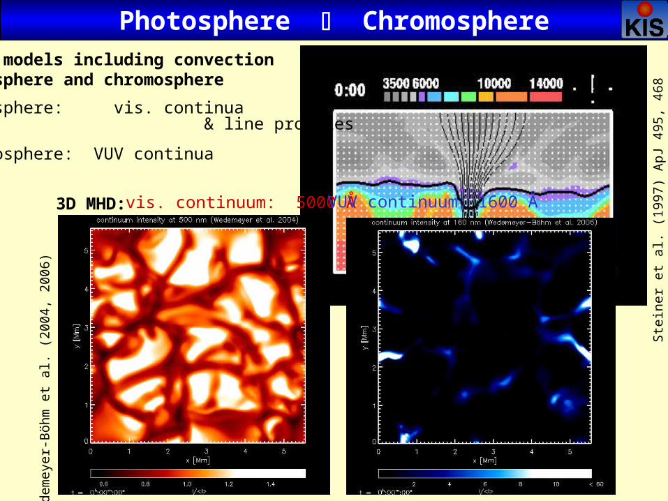
(M)HD models including convectionphotosphere and chromosphere

photosphere: vis. continua & line profiles

chromosphere: VUV continua

vis. continuum: 5000 Å VUV continuum: 1600 Å

Ste

iner

et

al.

(199

7) A

pJ 4

95,

468

"old" 2D flux tube

3D MHD:

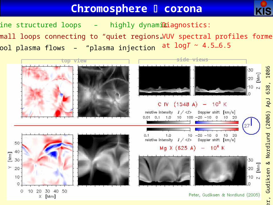
Chromosphere corona

side viewstop view

fine structured loops – highly dynamic

small loops connecting to “quiet regions”

cool plasma flows – “plasma injection”

Diagnostics:

VUV spectral profiles formedat logT ~ 4.5…6.5

Pet

er,

Gud

ikse

n &

No

rdlu

nd (

2006

) A

pJ 6

38,

108

6

The whole thing: convection corona

3D modelfrom theconvection zoneto the chromosphere

5.5 x 5.5 x 3 Mm (grid: 140x140x200)

x = y = 40 kmz = 50...12 km

vertical cut:5.5 x 3 Mm

coronal emission linefrom 3D MHD model

60 x 60 x 34 Mm (grid: 1503)

x = y = 400 kmz = 400...150 km

vertical cut:60 x 34 Mm

modeling the full system will not be possible very soon (box size 1500 x 1500 x 500) two step process: convection zone – photosphere – chromosphere chromosphere – corona but in time: large models from convection corona

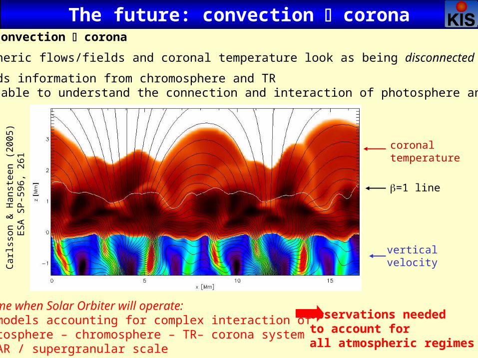
The future: convection corona

At time when Solar Orbiter will operate:3D models accounting for complex interaction ofphotosphere – chromosphere – TR– corona systemon AR / supergranular scale

Observations needed to account forall atmospheric regimes !!

Car

lsso

n &

Han

stee

n (2

005)

ES

A S

P-5

96,

261

2D model convection corona

photospheric flows/fields and coronal temperature look as being disconnected

one needs information from chromosphere and TR to be able to understand the connection and interaction of photosphere and corona

coronal temperature

verticalvelocity

=1 line





consequences


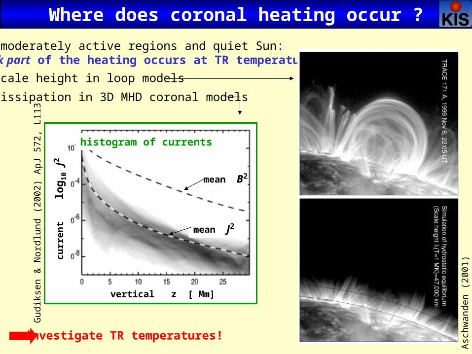
vertical z [ Mm]

curr

ent

lo

g 10 J

2

mean B2

mean J2

histogram of currents

Where does coronal heating occur ?

in moderately active regions and quiet Sun:bulk part of the heating occurs at TR temperatures

– scale height in loop models – dissipation in 3D MHD coronal models

investigate TR temperatures!

Gud

ikse

n &

Nor

dlun

d (2

002)

ApJ

572

, L1

13

Asc

hwan

den

(200

1)

Coronal heating and TR explosive events

Si IV (1393 Å) ~105 K ~10 min

200 km/s

~25

’’

SUMER

sola

r Y

from a time series 28.3.1996~1 min cadence (originally ~10 s)

transient broadening of TR emission lines, sometimes distinct emission peaks visible (e.g. Dere et al.,1989, Sol. Phys. 123, 41)

interpreted as bi-directional jets after reconnection (e.g. Innes et al., 1997, Nat. 386, 811)

explosive events are restricted to TR temperatures

how are they related to the dissipation of energy in the 3D MHD flux-braiding coronal models?

high spatial & spectral resolution TR line profiles needed

Propagation from chromosphere into corona

10

6

4

2

0

8

20 40 60 80 100position along the slit [arcsec]

time

[103

sec]

continuum C II: shift O VI: Int

Wikstøl et al. (2000) ApJ 531,1150

oscillations are present in line shift and intensity 5-10 mHz oscillations can be followed up from the chromosphere into the transition region

continuum

C II: shift

O VI: Int3 min

continuous informationfrom chromosphere TRis needed

Doppler shifts in the low corona & TRP

eter

& J

udge

(19

99)

ApJ

52

2, 1

148

mean quiet SunDoppler shiftsat disk center

net redshift in transition region

net blueshift in corona

in active region similar but with higher amplitude

SUMER

need for highspectral resolution > 30 000to get 1 km/s

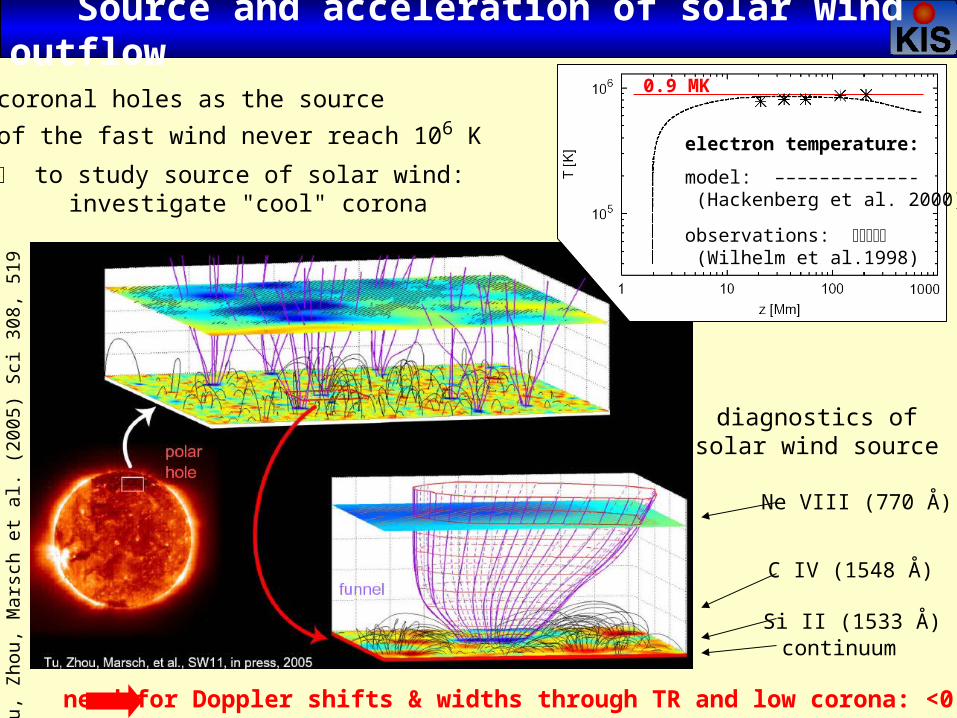
Source and acceleration of solar wind outflow

need for Doppler shifts & widths through TR and low corona: <0.9 MK

coronal holes as the source

of the fast wind never reach 106 K

to study source of solar wind: investigate "cool" corona

Tu,

Zho

u, M

arsc

h et

al.

(20

05)

Sci

308

, 51

9

electron temperature:

model: ––––––––––––- (Hackenberg et al. 2000)

observations: (Wilhelm et al.1998)

0.9 MK

Ne VIII (770 Å)

C IV (1548 Å)

Si II (1533 Å)continuum

diagnostics ofsolar wind source

Response of the atmosphere to energetic events

YohkohSXT

TRACE 195A

SUMER slit

Si III0.05 MK

Ca X0.7 MK

Ne VI0.3 MK

Fe XIX6.3 MK

Fe XIXline shift

Fe XVII2.8 MK

Ca XIII2.0 MK

Ca X0.7 MK

Fe XIX6.3 MK

follow dynamiccooling phaseof an energetic event

e.g. SUMER: 1100 – 1140 Å

spanning log T = 4.7 … 6.8

cover large temperature intervalto study response to energetic events

Coronal loop oscillations

Cur

dt e

t al

. (2

005)

ES

A S

P 5

92,

475

time

spac

e

1112 – 1120 Å





consequences


EUI

Photosphere imaging vis. / G-band

IR + vis spectropolarimetry: vector B

Chromosphere Ca II H + K / H

He I (10830 Å) vector B

EUV continua ~1000 – 1600 Å

transition region emission line spectra

VUV Dopplergrams for C IV (VUV-FPI ?)

corona emission line spectra

VUV / EUV imaging [ logT = 4…6.5 ]

X-ray imaging [ logT > 6 ]

Diagnostics through the atmosphere

EUS

VIM

"Interaction" of orbiter instruments

VIM – photospheric vector magnetic fields

provides photospheric flows and vector magnetic fields will be specially designed also to be able to provide

reliable magnetic field information suited for coronal field extrapolation huge efforts for reliable extrapolations, e.g. at MPS Lindau

EUI – chromospheric coronal imaging

provides VUV images: logT = ~4 (Ly ?) provides EUV images: logT = >6 (171 Å?)

EUS

should cover parts of the solar atmosphere also

accessible to the other instruments

close the gap in the atmosphere, the imaging instruments cannot cover

provide information on flows and densities where other instruments operate

Diagnostic needs interaction chromosphere – corona

– chromospheric continua ( > 912 Å / Ly–edge )

chromosphere – TR – corona system

– propagation of waves – plasma properties through atmosphere: line shifts, widths

dissipation of energy to heat corona

– TR dynamics and explosive events: spectral profiles – chromospheric and coronal response

coronal holes at high latitudes: source of solar wind

– in coronal holes: T<106 K – to get acceleration: T=105…106 K

energetic events

– cover large temperature range

good spectral resolution: > 30 000

– line profile details and Doppler shifts down to 1 km/s

longer wavelengths:"easier" to get goodspectral resolution:e.g. 1 km/s =Ne VIII 770 Å : 10 mÅ Fe IX 171 Å : 2 mÅ

only >912 Åallows to reachtemperature minimum

e.g.:Mg X 609 / 625 Å Ne VIII 770 / 780 ÅN V 1239 / 1243 ÅC III 977 / 1175 Å

v < 5 km/s

only then loop flows,CH outflow andprofile details e.g. forexplosive events

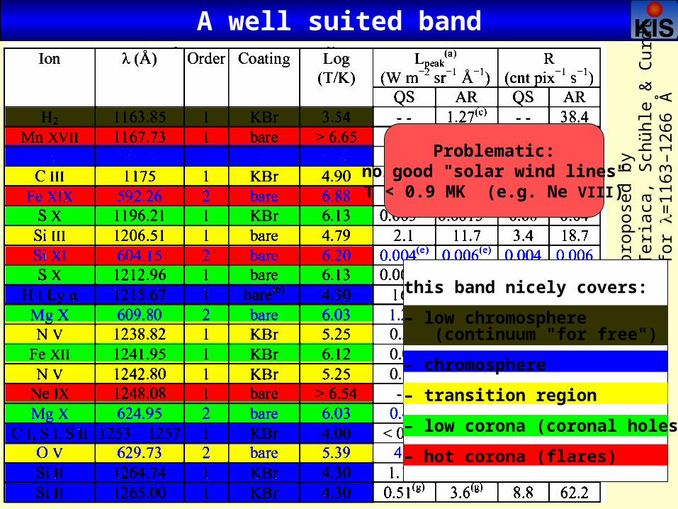
A well suited band

prop

osed

by

Ter

iaca

, S

chüh

le &

Cur

dtfo

r =

1163

–126

6 Å

this band nicely covers:

– low chromosphere (continuum "for free")

– chromosphere

– transition region

– low corona (coronal holes)

– hot corona (flares)

Problematic:no good "solar wind lines"

T < 0.9 MK (e.g. Ne VIII)

Conclusions

Solar Orbiter provides

unique opportunity to study the complex interactions of the

photosphere – chromosphere – TR – corona – heliosphere system

in order to ideally complement the other instruments (EUI/VIM)

EUS has to cover the chromosphere – TR – corona system

it is not sufficient to cover only hot temperature plasma:

models need information also on chromosphere – TR system

if one misses out the chromosphere – TR system,

there will be a serious ambiguity in checking future models

for the dynamics and heating of the corona

Thanks for replacing the LAMP.

not to be used…

3D MHD model for the corona: 50 x 50 x 30 Mm Box (1503) – fully compressible; high order – non-uniform mesh

full energy equation (heat conduction, rad. losses)

starting with scaled-down MDI magnetogram – no emerging flux

photospheric driver: foot-point shuffled by convection

braiding of magnetic fields (Galsgaard, Nordlund 1995; JGR 101, 13445)

heating: DC current dissipation (Parker 1972; ApJ 174, 499)

heating rate j2 ~ exp(- z/H )

loop-structured 106K corona

Gudiksen & Nordlund (2002) ApJ 572, L113 (2005) ApJ 618, 1020 & 1031Bingert, Peter, Gudiksen & Nordlund (2005)

3D MHD coronal modeling

horizontal x [ Mm]

ho

rizo

nta

l

y [

Mm

]

MDI magnetogram

vertical z [ Mm]

curr

ent

lo

g 10 J

2

mean B2

mean J2

histogram of currents

0 10 20 30 40

10

20

horizontal X [Mm]

ve

rtic

al

Z

[Mm

]

Bin

ger

t et

al.

(200

5)“emission” @ 106 K

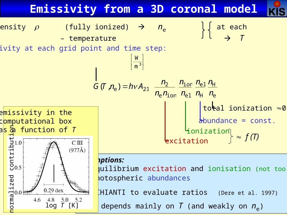
21e ),( AhnTG ione

2

nn

n

el

ion

n

n

e

H

n

n

H

el

n

n

3m

W

total ionization 0.8

abundance = const.

ionizationexcitation

Assumptions:– equilibrium excitation and ionisation (not too bad...)

– photospheric abundances

use CHIANTI to evaluate ratios (Dere et al. 1997) G depends mainly on T (and weakly on ne) log T [K]

norm

aliz

ed c

ontr

ibut

ion

emissivity in the computational box as a function of T

From the MHD model: – density (fully ionized) ne at each

– temperature T grid point and time

Emissivity from a 3D coronal model

Emissivity at each grid point and time step:

f (T)

DEM inversion using CHIANTI:

1 – using synthetic spectra derived from 3D MHD model

2 – using solar observations (SUMER, same lines)

Emission measure

T

hnDEM

d

d2e

Si II Mg X

Supporting suggestions thatnumerous cool structures

cause increase of DEM to low T

1D loop model – flatgood match to observations!!DEM increases towards low T in the model !

The whole thing: convection corona: a problem

3D modelfrom theconvection zoneto the chromosphere

5.5 x 5.5 x 3 Mm (grid: 140x140x200)

x = y = 40 kmz = 50...12 km

vertical cut:5.5 x 3 Mm

coronal emission linefrom 3D MHD model

60 x 60 x 34 Mm (grid: 1503)

x = y = 400 kmz = 400...150 km

vertical cut:60 x 34 Mm

2

4

6

8

10

12

14

16

tem

pera

ture

[

100

0 K

]

Wed

emey

er e

t al

. (2

004)

A&

A 4

14,

11

21

modeling the full system will not be possible very soon (box size 1500 x 1500 x 500) two step process: convection zone – photosphere – chromosphere chromosphere – corona but in time: large models from convection corona

Science drivers for wavelength selection: Quiet Sun and Active regions Hardi Peter...

Documents

Transcript of Science drivers for wavelength selection: Quiet Sun and Active regions Hardi Peter...